Electrical Power and Energy Systems 54 (2014) 10–16

Contents lists available at SciVerse ScienceDirect

Electrical Power and Energy Systems

journal homepage: www.elsevier .com/locate / i jepes

Modelling major failures in power grids in the whole range

0142-0615/$ - see front matter � 2013 Elsevier Ltd. All rights reserved.http://dx.doi.org/10.1016/j.ijepes.2013.06.033

⇑ Corresponding author. Tel.: +34 942 206758; fax: +34 942 201603.E-mail address: faustino.prieto@unican.es (F. Prieto).

Faustino Prieto a,⇑, José María Sarabia a, Antonio José Sáez b

a Department of Economics, University of Cantabria, Avenida de los Castros s/n, 39005 Santander, Spainb Department of Statistics and Operations Research, Polytechnic School of Linares, University of Jaén, C/Alfonso X El Sabio 28, 23700 Linares (Jaén), Spain

a r t i c l e i n f o

Article history:Received 23 January 2013Received in revised form 6 June 2013Accepted 29 June 2013

Keywords:Electricity transmission networksComplex SystemsPower lawPareto IILomaxBootstrap

a b s t r a c t

Empirical research with electricity transmission networks reliability data shows that the size of majorfailures – in terms of energy not supplied (ENS), total loss of power (TLP) or restoration time (RT) – appearto follow a power law behaviour in the upper tail of the distribution. However, this pattern (also knownas Pareto distribution) is not valid in the whole range of those major events. We aimed to find a proba-bility distribution that we could use to model them, and hypothesized that there is a two-parametermodel that fits the pattern of those data well in the entire domain. We considered the major failures pro-duced between 2002 and 2012 in the European power grid; analyzed those reliability indicators: ENS, TLPand RT; fitted six alternative models: Pareto II, Fisk, Lognormal, Pareto, Weibull and Gamma distributions,to the data by maximum likelihood; compared these models by the Bayesian information criterion;tested the goodness-of-fit of those models by a Kolmogorov–Smirnov test method based on bootstrapresampling; and validated them graphically by rank-size plots. We found that Pareto II distribution is,in the case of TLP, an adequate model to describe major events reliability data of power grids in the wholerange, and in the case of ENS and RT, is the best choice of the six alternative models analyzed.

� 2013 Elsevier Ltd. All rights reserved.

1. Introduction

Electricity transmission networks provide the means to trans-port the electricity from the power plants, where is produced, tothe distribution networks, near our homes and businesses. Unfor-tunately, failures in these systems do happen [1], and nowadays,electricity is essential for all of us [2,3]. For that reason, the analysisof those failure events, in particular from a statistical point of view,is crucial to improve the reliability of those transmission infra-structures [4,5] – the resulting probability distribution can helpus to understand the underlying data generating process [6].

In this direction, some promising results have been obtainedusing network reliability data from major events: the number ofcustomers affected by electrical blackouts in the United States be-tween 1984 and 2002 [7]; the energy not supplied, the total loss ofpower and the restoration time in the European power grid be-tween 2002 and 2008 [8], all can be fitted by a power law distribu-tion (also known as Pareto distribution [9,10]) in the upper tail ofthe distribution.

However, this power law behaviour is not valid in the wholerange of those datasets analyzed. The number of observations in-cluded in the power-law upper tail is small. As examples, onlythe 15% of the major events for energy not supplied and less than10% of the major events for total loss of power datasets mentioned

in Ref. [8] follow that power law behaviour, giving us the evidencethat power law model is unable to describe the behaviour of thehigh, medium and low ranges of those data at the same time.

The aim of this study was to find a probability distribution thatwe could use to model major events reliability data of electricitytransmission networks in the whole range, and that we could useas a starting point for further study of the power grid dynamicsconsidering all the amount of major events. Our primary hypothe-sis was that there is a two-parameter model that fits the pattern ofdata well – following the principle of parsimony and admittingmore than two parameters only if necessary. As candidate models,we considered the Pareto II, the Fisk, the Lognormal, the Weibulland the Gamma distributions, which were analyzed together withthe pareto (power law) model. We found that Pareto II (Lomax)distribution is a good alternative for modelling power grid reliabil-ity data, in the entire domain of the major events.

The rest of this paper is organized as follows: in Section 2, weintroduce the datasets analyzed and the method used; the resultsare presented and discussed afterwards in Section 3; finally, theconclusions are in Section 4.

2. Data and methods

We considered the network reliability data from Union for Co-ordination of Transmission of Electricity (UCTE) [11] – in 2007,as a reference, an association of 29 transmission system operatorsof 24 european countries, with an installed capacity of 640 GW, an

Table 1Main empirical characteristics of ENS, TLP and RT, from major events of UCTE electricity transmission network, between January 2002 and December 2009.

n Mean Std. dev. Skewness Kurtosis Min. Max.

ENS 2002–2009 (MW h) 583 631.17 7133.86 22.31 521.74 1 168,000TLP 2002–2009 (MW) 528 374.41 1431.23 12.05 178.26 1 24,120RT 2002–2009 (min) 689 493.36 3290.20 10.88 134.03 1 50,432

Table 3Cumulative distribution functions and probability density functions used; c(a,x/r)represents the lower incomplete gamma function.

Distribution F(x) f(x)

Pareto II 1� xþrr

� ��a ara

ðxþrÞaþ1 , x P 0

Fisk 11þðx=aÞ�b

ðb=aÞðx=aÞb�1

ð1þðx=aÞbÞ2, x > 0

Lognormal U log x�lr

� �1

xrffiffiffiffiffi2pp exp � ðlog x�lÞ2

2r2

h i, x > 0

Pareto (PowerLaw) 1� xr� ��a ara

xaþ1, x P rWeibull 1� exp � x

k

� �bh ibk

� �xk

� �b�1 exp � xk

� �bh i, x P 0

Gamma 1CðaÞ c a; x

r� �

1CðaÞra xa�1 exp � x

r� �

, x > 0

F. Prieto et al. / Electrical Power and Energy Systems 54 (2014) 10–16 11

electricity consumption of 2600 TW h, a length of high-voltagetransmission lines managed of 220,000 km and 500 million peopleserved. The first dataset considered in this work consists of a ran-dom sample of major events, between January 2002 and December2009, from UCTE, with Energy not Supplied (ENS 2002–2009) givenin MW h, Total Loss of Power (TLP 2002–2009) given in MW, andRestoration Time (RT 2002–2009) given in minutes, and wherezero values have not been considered. This dataset was describedbefore in Ref. [8], contains 698 major events, and can be found inRef. [12]. Table 1 shows the main empirical characteristics of ENS2002–2009, TLP 2002–2009 and RT 2002–2009.

In 2009, all UCTE operation tasks were transferred to the Euro-pean Network of Transmission System Operators for Electricity(ENTSO-E) [13]. Nowadays, ENTSO-E is an association of 41 trans-mission system operators of 34 european countries, included thosefrom UCTE and from other predeccesor associations like ATSOI,BALTSO, NORDEL, ETSO and UKTSOA – in 2011, as a reference, with880GW net generation capacity, an electricity consumption of3200 TW h, a length of high-voltage transmission lines managedof 305,000 km and 53 million customers served. The second data-set considered in this work corresponds to a random sample of ma-jor events, between January 2002 and December 2012, from UCTE(2002–2009) and from ETSO-E (2010–2012), with Energy not Sup-plied (ENS 2002–2012) expressed in MW h, Total Loss of Power(TLP 2002–2012) expressed in MW, and Restoration Time (RT2002–2012) expressed in minutes, and where zero values havenot been considered. This dataset contains 886 major events, in-cludes the first dataset considered, and can be found in Ref. [14].Table 2 shows the main empirical characteristics of ENS 2002–2012, TLP 2002–12 and RT 2002–2012.

We fitted and compared six models with two parameters: thePareto II distribution (also known as Lomax distribution) [10,15],the Fisk distribution (also known as Log–logistic distribution)[16], the Lognormal distribution [17], the Pareto (Power law) dis-tribution, the Weibull distribution [18] and the Gamma distribu-tion [19]. Table 3 shows the cumulative distribution functionsF(x) and the probability density functions f(x) of these sixdistributions.

First, we fitted all six models by maximum likelihood [19]. Foreach model, the log-likelihood function is given by

log ‘ðhjxÞ ¼Xn

i¼1

log f ðxijhÞ; ð1Þ

where h is the unknown parameter vector of the model, x is thesample data, f(x) is its probability density function showed inTable 3, and the maximum likelihood estimation of the parametervector h is the one that maximizes the likelihood function log l(h/x).

Table 2Main empirical characteristics of ENS, TLP and RT, from major events of UCTE (Januartransmission networks.

n Mean Std. dev.

ENS 2002–2012 (MW h) 744 552.35 6368.25TLP 2002–2012 (MW) 699 307.76 1252.41RT 2002–2012 (min) 872 418.79 2930.55

Then, we compared those models using the following modelselection criteria: the Akaike information criterion (AIC), definedby [20]

AIC ¼ �2 log Lþ 2d; ð2Þ

and the Bayesian information criterion (BIC), defined by [21]

BIC ¼ log L� 12

d log n; ð3Þ

where log L ¼ log ‘ðhjxÞ is the log-likelihood (see Eq. (1)) of the mod-el evaluated at the maximum likelihood estimates, d is the numberof parameters, n is the number of data, and the model chosen is theone with the smallest value of AIC statistic or with the largest valueof BIC statistic.

After that, we tested the goodness-of-fit of all the six modelsconsidered by a Kolmogorov–Smirnov (KS) test method based onbootstrap resampling [7,22–25]. Let x1, x2, . . . , xn be the sampleof X and

FnðxiÞ �1

nþ 1

Xn

j¼1

I½xj6xi �

be the empirical cumulative distribution function (cdf) in a samplevalue with the indicated plotting position formula [26]. Let Fðx; hÞbe the theoretical cdf of a particular model fitted by maximum like-lihood. The KS statistic of the model is given by [27,28]

Dn ¼ sup jFnðxiÞ � Fðxi; hÞj; i ¼ 1;2; . . . ;n; ð4Þ

and the null hypothesis to test is H0: the data follow that model.Then, for each model, the procedure is as follows: (1) calculatethe empirical KS statistic for the observed data; (2) generate, bysimulation, enough synthetic data sets (in this study, we generated10,000 data sets), with the same sample size n as the observed data– if U is uniformly distributed on [0,1] and Qðp; hÞ is the theoretical

y 2002–December 2009) and ENTSO-E (January 2010–December 2012) electricity

Skewness Kurtosis Min. Max.

24.65 644.72 0.3 168,00013.73 232.34 1 24,12012.24 169.41 1 50,432

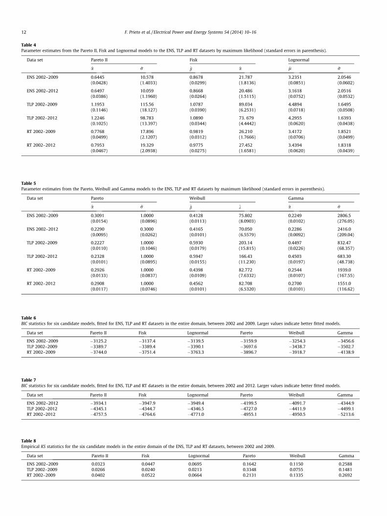
Table 4Parameter estimates from the Pareto II, Fisk and Lognormal models to the ENS, TLP and RT datasets by maximum likelihood (standard errors in parenthesis).

Data set Pareto II Fisk Lognormal

a r b a l r

ENS 2002–2009 0.6445 10.578 0.8678 21.787 3.2351 2.0546(0.0428) (1.4033) (0.0299) (1.8136) (0.0851) (0.0602)

ENS 2002–2012 0.6497 10.059 0.8668 20.486 3.1618 2.0516(0.0386) (1.1960) (0.0264) (1.5115) (0.0752) (0.0532)

TLP 2002–2009 1.1953 115.56 1.0787 89.034 4.4894 1.6495(0.1146) (18.127) (0.0390) (6.2531) (0.0718) (0.0508)

TLP 2002–2012 1.2246 98.783 1.0890 73. 679 4.2955 1.6393(0.1025) (13.397) (0.0344) (4.4442) (0.0620) (0.0438)

RT 2002–2009 0.7768 17.896 0.9819 26.210 3.4172 1.8521(0.0499) (2.1207) (0.0312) (1.7666) (0.0706) (0.0499)

RT 2002–2012 0.7953 19.329 0.9775 27.452 3.4394 1.8318(0.0467) (2.0938) (0.0275) (1.6581) (0.0620) (0.0439)

Table 5Parameter estimates from the Pareto, Weibull and Gamma models to the ENS, TLP and RT datasets by maximum likelihood (standard errors in parenthesis).

Data set Pareto Weibull Gamma

a r b k a r

ENS 2002–2009 0.3091 1.0000 0.4128 75.802 0.2249 2806.5(0.0154) (0.0896) (0.0113) (8.0903) (0.0102) (276.05)

ENS 2002–2012 0.2290 0.3000 0.4165 70.050 0.2286 2416.0(0.0095) (0.0262) (0.0101) (6.5579) (0.0092) (209.04)

TLP 2002–2009 0.2227 1.0000 0.5930 203.14 0.4497 832.47(0.0110) (0.1046) (0.0179) (15.815) (0.0226) (68.357)

TLP 2002–2012 0.2328 1.0000 0.5947 166.43 0.4503 683.30(0.0101) (0.0895) (0.0155) (11.230) (0.0197) (48.738)

RT 2002–2009 0.2926 1.0000 0.4398 82.772 0.2544 1939.0(0.0133) (0.0837) (0.0109) (7.6332) (0.0107) (167.55)

RT 2002–2012 0.2908 1.0000 0.4562 82.708 0.2700 1551.0(0.0117) (0.0746) (0.0101) (6.5320) (0.0101) (116.62)

Table 6BIC statistics for six candidate models, fitted for ENS, TLP and RT datasets in the entire domain, between 2002 and 2009. Larger values indicate better fitted models.

Data set Pareto II Fisk Lognormal Pareto Weibull Gamma

ENS 2002–2009 �3125.2 �3137.4 �3139.5 �3159.9 �3254.3 �3456.6TLP 2002–2009 �3389.7 �3389.4 �3390.1 �3697.6 �3438.7 �3502.7RT 2002–2009 �3744.0 �3751.4 �3763.3 �3896.7 �3918.7 �4138.9

Table 7BIC statistics for six candidate models, fitted for ENS, TLP and RT datasets in the entire domain, between 2002 and 2012. Larger values indicate better fitted models.

Data set Pareto II Fisk Lognormal Pareto Weibull Gamma

ENS 2002–2012 �3934.1 �3947.9 �3949.4 �4199.5 �4091.7 �4344.9TLP 2002–2012 �4345.1 �4344.7 �4346.5 �4727.0 �4411.9 �4499.1RT 2002–2012 �4757.5 �4764.6 �4771.0 �4955.1 �4950.5 �5213.6

Table 8Empirical KS statistics for the six candidate models in the entire domain of the ENS, TLP and RT datasets, between 2002 and 2009.

Data set Pareto II Fisk Lognormal Pareto Weibull Gamma

ENS 2002–2009 0.0323 0.0447 0.0695 0.1642 0.1150 0.2588TLP 2002–2009 0.0266 0.0240 0.0213 0.3348 0.0755 0.1481RT 2002–2009 0.0402 0.0522 0.0664 0.2131 0.1335 0.2692

12 F. Prieto et al. / Electrical Power and Energy Systems 54 (2014) 10–16

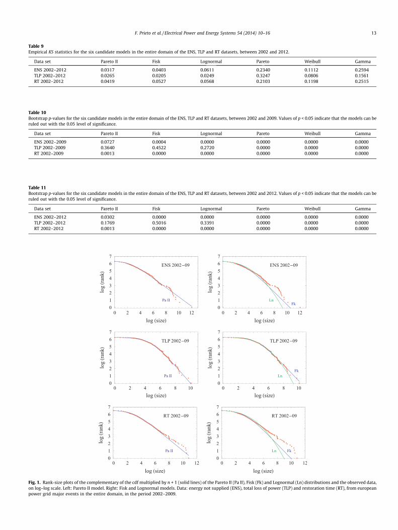
Table 9Empirical KS statistics for the six candidate models in the entire domain of the ENS, TLP and RT datasets, between 2002 and 2012.

Data set Pareto II Fisk Lognormal Pareto Weibull Gamma

ENS 2002–2012 0.0317 0.0403 0.0611 0.2340 0.1112 0.2594TLP 2002–2012 0.0265 0.0205 0.0249 0.3247 0.0806 0.1561RT 2002–2012 0.0419 0.0527 0.0568 0.2103 0.1198 0.2515

Table 10Bootstrap p-values for the six candidate models in the entire domain of the ENS, TLP and RT datasets, between 2002 and 2009. Values of p < 0.05 indicate that the models can beruled out with the 0.05 level of significance.

Data set Pareto II Fisk Lognormal Pareto Weibull Gamma

ENS 2002–2009 0.0727 0.0004 0.0000 0.0000 0.0000 0.0000TLP 2002–2009 0.3640 0.4522 0.2720 0.0000 0.0000 0.0000RT 2002–2009 0.0013 0.0000 0.0000 0.0000 0.0000 0.0000

Table 11Bootstrap p-values for the six candidate models in the entire domain of the ENS, TLP and RT datasets, between 2002 and 2012. Values of p < 0.05 indicate that the models can beruled out with the 0.05 level of significance.

Data set Pareto II Fisk Lognormal Pareto Weibull Gamma

ENS 2002–2012 0.0302 0.0000 0.0000 0.0000 0.0000 0.0000TLP 2002–2012 0.1769 0.5016 0.3391 0.0000 0.0000 0.0000RT 2002–2012 0.0013 0.0000 0.0000 0.0000 0.0000 0.0000

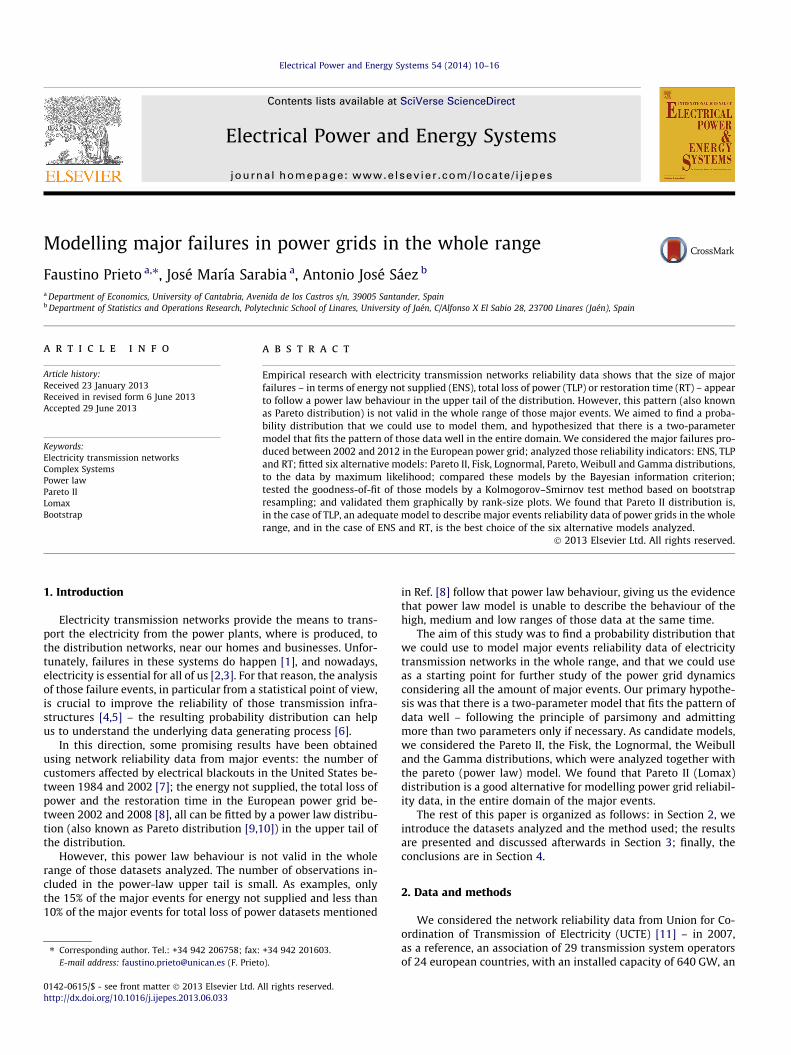
Fig. 1. Rank-size plots of the complementary of the cdf multiplied by n + 1 (solid lines) of the Pareto II (Pa II), Fisk (Fk) and Lognormal (Ln) distributions and the observed dataon log–log scale. Left: Pareto II model. Right: Fisk and Lognormal models. Data: energy not supplied (ENS), total loss of power (TLP) and restoration time (RT), from europeanpower grid major events in the entire domain, in the period 2002–2009.

F. Prieto et al. / Electrical Power and Energy Systems 54 (2014) 10–16 13

,

14 F. Prieto et al. / Electrical Power and Energy Systems 54 (2014) 10–16

quantile function of the model, then QðU; hÞ has that model distri-bution; (3) fit each synthetic data set by maximum likelihood andobtained its theoretical cdf; (4) calculate the KS statistic for eachsynthetic data set – with its own theoretical cdf; (5) calculate thep-value as the fraction of synthetic data sets with a KS statisticgreater than the empirical KS statistic; and (6) null hypothesis canbe rejected at the 0.05 level of significance if p-value <0.05 [see Refs.[6,7].

Finally, as a graphical model validation, we used a rank-size plot(on a log–log scale). Let x(1) 6 x(2) 6 � � � 6 x(n) be the ordered sampleof X, we considered the scatter plot of the points (observed data)

log½ranki� versus log½xðiÞ�; i ¼ 1;2; . . . ;n; ð5Þ

where ranki = n + 1 � i = (n + 1)(1 � Fn(x(i))), plotted it together withthe complementary of the theoretical cdf of the model multiplied by(n + 1)

log½ðnþ 1Þð1� FðxðiÞ; hÞÞ� versus log½xðiÞ�; i ¼ 1;2; . . . ;n; ð6Þ

and evaluated graphically how well the model fitted the observeddata.

3. Results and discussion

Tables 4 and 5 show the parameter estimates and their standarderrors from the six alternative models considered: the Pareto II dis-tribution (a and r parameters); the Fisk distribution (b and aparameters); the Lognormal distribution (l and r parameters);the Pareto (power law) distribution (a and r parameters); the Wei-bull distribution (b and k parameters) and the Gamma distribution

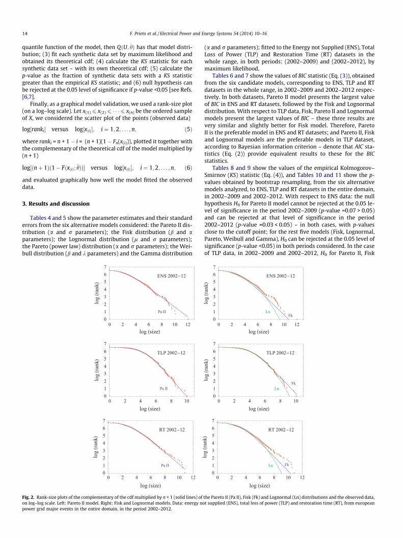
Fig. 2. Rank-size plots of the complementary of the cdf multiplied by n + 1 (solid lines) ofon log–log scale. Left: Pareto II model. Right: Fisk and Lognormal models. Data: energy nopower grid major events in the entire domain, in the period 2002–2012.

(a and r parameters); fitted to the Energy not Supplied (ENS), TotalLoss of Power (TLP) and Restoration Time (RT) datasets in thewhole range, in both periods: (2002–2009) and (2002–2012), bymaximum likelihood.

Tables 6 and 7 show the values of BIC statistic (Eq. (3)), obtainedfrom the six candidate models, corresponding to ENS, TLP and RTdatasets in the whole range, in 2002–2009 and 2002–2012 respec-tively. In both datasets, Pareto II model presents the largest valueof BIC in ENS and RT datasets, followed by the Fisk and Lognormaldistribution. With respect to TLP data, Fisk, Pareto II and Lognormalmodels present the largest values of BIC – these three results arevery similar and slightly better for Fisk model. Therefore, ParetoII is the preferable model in ENS and RT datasets; and Pareto II, Fiskand Lognormal models are the preferable models in TLP dataset,according to Bayesian information criterion – denote that AIC sta-tistics (Eq. (2)) provide equivalent results to these for the BICstatistics.

Tables 8 and 9 show the values of the empirical Kolmogorov–Smirnov (KS) statistic (Eq. (4)), and Tables 10 and 11 show the p-values obtained by bootstrap resampling, from the six alternativemodels analyzed, to ENS, TLP and RT datasets in the entire domain,in 2002–2009 and 2002–2012. With respect to ENS data: the nullhypothesis H0 for Pareto II model cannot be rejected at the 0.05 le-vel of significance in the period 2002–2009 (p-value =0.07 > 0.05)and can be rejected at that level of significance in the period2002–2012 (p-value =0.03 < 0.05) – in both cases, with p-valuesclose to the cutoff point; for the rest five models (Fisk, Lognormal,Pareto, Weibull and Gamma), H0 can be rejected at the 0.05 level ofsignificance (p-value <0.05) in both periods considered. In the caseof TLP data, in 2002–2009 and 2002–2012, H0 for Pareto II, Fisk

the Pareto II (Pa II), Fisk (Fk) and Lognormal (Ln) distributions and the observed data,t supplied (ENS), total loss of power (TLP) and restoration time (RT), from european

F. Prieto et al. / Electrical Power and Energy Systems 54 (2014) 10–16 15

and Log-normal models cannot be rejected and for Pareto, Weibulland Gamma models can be rejected at the 0.05 level. Finally, H0 forall the six candidate models can be rejected at the 0.05 level ofsignificance in the cases of RT 2002–2009 and RT 2002–2012datasets.

Rank-size plots (defined by expressions Eqs. (5) and (6), corre-sponding to the whole range of major events, in the two periodsconsidered 2002–2009 and 2002–2012, of Energy not Supplied(ENS, in MW h), Total Loss of Power (TLP, in MW) and RestorationTime (RT, in minutes) datasets, show graphically (see Figs. 1 and2): the adequacy of the Pareto II, Fisk and Lognormal models tothe TLP dataset; and the best description of the ENS and RT datasetgiven by the Pareto II model in comparison with Fisk and Lognor-mal models.

In summary, according to the results obtained, Pareto II, Fiskand Lognormal distribution may serve as an adequate model forTotal Loss of Power data from major failures in Electricity Trans-mission Networks in the entire domain, against other alternativemodels such as Pareto (power law), Weibull and Gamma distribu-tions. Adittionally, Pareto II distribution fits reasonably wellEnergy Not Supplied and Restoration Time data but with somedeviation, improving other alternative models such as Fisk, Log-normal, Pareto, Weibull and Gamma distribution – unfortunately,these deviations are statistically significant. Note that Pareto IIdistribution is a shifted power law distribution, which turns intoa Pareto distribution for large values of the variable [29], follow-ing the known power law behaviour in the upper tail, and hasonly two parameters which means simplicity. Pareto II distribu-tion has been used in another contexts, for example, with busi-ness failure data [15]; with the biomass size spectrum [30]; and,according to Ref. [10], Pareto II distribution is well adapted formodelling reliability problems [31]. Finally, Pareto II distributionis also supported from a theoretical point of view. In this sense,there are two stochastic mechanisms which lead to thisdistribution:

(a) This distribution can be obtained by introducing a frailtyparameter in the basic survival function S0(x) = (1 + x/r)�1,using the formulation S(x;a) = [S0(x)]a [see Ref. 32, chap.11].

(b) On the other hand, the Pareto II arises also as a limiting dis-tribution in record value contexts [see Ref. 10]. Consider asequence of independent identically distributed randomvariables X1, X2, . . . with continuous common distribution.Now, we fix integers k and n with k < n, and define the ran-dom variable Zk given by

Zk ¼minfm : m P 1;Xmþn > Xn�kþ1:ng;

where Xi:n denotes the ith order statistics in a sample of size n. Then,Zk is the waiting time after taking n observations until we get anobservation bigger than the kth largest of the first n observations.One can show that for n large, the random variable Zk/n is approx-imately distributing according a Pareto II distribution with shapeparameter k, that is, if [x] denotes the integer part of x [see Ref.10, chap. 3],

limn!1

PrðZk=n > xÞ ¼ limn!1

PrðZk > ½nx�Þ ¼ 1

ð1þ xÞk;

with x > 0, which coincides with Pareto II distribution in Table 3with r = 1 and a = k.

For all of that, we think that Pareto II (Lomax) distribution is agood alternative for modelling power grid reliability data, in theentire domain of the major events.

4. Conclusions

We found a two parameter probability distribution that we canuse to model major events reliability data of electricity transmis-sion networks in the entire domain: the Pareto II distribution – alsoknown as Lomax distribution.

Pareto II model fits very well the pattern of Total Loss of Power(TLP) data and is the best of the six models considered for Energynot Supplied (ENS) and Restoration Time (RT) data. Additionally,we found other two models with two parameters: the Fisk (alsoknown as Log–logistic distribution) and the Lognormal distribu-tions, adequate specifically for Total Loss of Power data.

We considered the major failures produced in the Europeanpower grid in the periods 2002–2009 (UCTE) and 2010–2012(ENTSO-E); analyzed three reliability indicators: ENS, TLP and RT;fitted six alternative models: Pareto II, Fisk, Lognormal, Pareto(PowerLaw), Weibull and Gamma distributions, to the data bymaximum likelihood; compared these models by the Bayesianinformation criterion; tested the goodness-of-fit of those modelsby a Kolmogorov–Smirnov test method based on bootstrap resam-pling; and validated them graphically by rank-size plots.

Future work is needed to confirm the validity of the Pareto IImodel for Energy not Supplied data and to find a better modelfor Restoration Time data from major failures in power grids inthe entire domain – with two parameters or three parameters ifnecessary.

Previous empirical research has shown that Pareto (power law)distribution is an adequate model to describe major events reliabil-ity data of electricity transmission networks in the upper tail. Inthis study we found that Pareto II distribution – a shifted powerlaw distribution – is a better choice to describe major events reli-ability data of electricity transmission networks in the entiredomain.

Acknowledgements

The authors thank to Ministerio de Economía y Competitividad(Project ECO2010-15455) for partial support of this work. Wethank Martí Rosas Casals for his assistance with data collection.We are grateful for the constructive suggestions provided by thereviewers, which improved the paper.

References

[1] Fairley P. The unruly power grid. IEEE Spectrum 2004;41(8):16–21.[2] Bompard E, Huang T, Wu Y, Cremenescu M. Classification and trend analysis of

threats origins to the security of power systems. Int J Electr Power Energy Syst2013;50:50–64.

[3] Chang L, Wu Z. Performance and reliability of electrical power grids undercascading failures. Int J Electr Power Energy Syst 2011;33:1410–9.

[4] Zio E. Reliability engineering: old problems and new challenges. Reliab EngSyst Saf 2009;94:125–41.

[5] Cupac V, Lizier JT, Prokopenko M. Comparing dynamics of cascading failuresbetween network-centric and power flow models. Int J Electr Power EnergySyst 2013;49:369–79.

[6] Mayo DG, Cox DR. Frequentist statistics as a theory of inductive inference. In:Mayo D, Spanos A, editors. Error and inference: recent exchanges onexperimental reasoning, reliability and the objectivity and rationality ofscience. Cambridge: Cambridge University Press; 2010. p. 1–27;. This paper appeared in The Second ErichLehmann L, editor. Symposium:optimality, lecture notes-monograph series, vol. 49. Institute of MathematicalStatistics; 2006. p. 247–75.

[7] Clauset A, Shalizi CR, Newman MEJ. Power-law distributions in empirical data.SIAM Rev 2009;51(4):661–703.

[8] Rosas-Casals M, Solé R. Analysis of major failures in Europe’s power grid. Int JElectr Power Energy Syst 2011;33:805–8.

[9] Pareto V. Cours d’Economie Politique. Rouge et Cie, Paris; 1897.[10] Arnold BC. Pareto distributions. Fairland, Maryland: International Co-operative

Publishing House; 1983.[11] https://www.entsoe.eu/fileadmin/user_upload/_library/publications/ce/

Statistical_Yearbook_2007.pdf.

16 F. Prieto et al. / Electrical Power and Energy Systems 54 (2014) 10–16

[12] https://www.entsoe.eu/publications/former-associations/ucte/monthly-statistics/.

[13] https://www.entsoe.eu/fileadmin/user_upload/_library/publications/entsoe/Factsheet/110202_Factsheet_2011.pdf.

[14] https://www.entsoe.eu/publications/monthly-statistics/.[15] Lomax KS. Business failures; another example of the analysis of failure data. J

Am Stat Assoc 1954;49:847–52.[16] Fisk PR. The graduation of income distributions. Econometrica

1961;29:171–85.[17] Johnson NL, Kotz S, Balakrishnan N. Continuous univariate distributions, vol.

1. New York: John Wiley; 1994.[18] Weibull W. A statistical distribution function of wide applicability. J Appl

Mech 1951;18(3):293–7.[19] Fisher RA. On the mathematical foundations of theoretical statistics. Philos

Trans Roy Soc Ser A 1922;222:309–68.[20] Akaike H. A new look at the statistical model identification. IEEE Trans Autom

Control 1974;19:716–23.[21] Schwarz G. Estimating the dimension of a model. Ann Stat 1978;5:461–4.[22] Efron B. Bootstrap methods: another look at the jackknife. Ann Stat

1979;7(1):1–26.[23] Wang C, Zeng B, Shao J. Application of bootstrap method in Kolmogorov–

Smirnov test. Qual Reliab Risk Maint Saf Eng (ICQR2MSE) 2011:287–91.

[24] Babu GJ, Rao CR. Goodness-of-fit tests when parameters are estimated.Sankhya 2004;66:63–74.

[25] Abbasi B, Guillen M. Bootstrap control charts in monitoring value at risk ininsurance. Expert Syst Appl, 2013.

[26] Castillo E, Hadi AS, Balakrishnan N, Sarabia JM. Extreme value and relatedmodels with applications in engineering and science. John Wiley & Sons; 2005[chap. 5].

[27] Kolmogorov AN. Sulla Determinazione Empirica di una Legge di Distribuzione.Giornale dell’Istituto degli Attuari 1933;4:83–91.

[28] Smirnov N. On the estimation of the discrepancy between empirical curves ofdistribution for two independent samples. Bulletin Mathematique del’Universite’ de Moscou, 2, fasc 2, 1939.

[29] Milojevic S. Power law distributions in information science: making the casefor logarithmic binning. J Am Soc Inform Sci Technol 2010;61(12):2417–25.

[30] Vidondo B, Prairie YT, Blanco JM, Duarte CM. Some aspects of the analysis ofsize spectra in aquatic ecology. Limnol Oceanogr 1997;42:184–92.

[31] Lemonte AJ, Cordeiro GM. An extended Lomax distribution. Statistics2011:1–17.

[32] Marshall AW, Olkin I. Life distributions structure of nonparametric,semiparametric, and parametric families. New York: Springer; 2007 [chap. 11].