Modelling failures in existing reinforced concretecolumns

Kenneth J. Elwood

Abstract: Experimental research and post-earthquake reconnaissance have demonstrated that reinforced concrete col-umns with light or widely spaced transverse reinforcement are vulnerable to shear failure, and in turn, axial failure dur-ing earthquakes. Based on experimental data, failure surfaces have been used to define the onset of shear and axialfailure for such columns. After the response of the column intersects the failure surface, the shear or axial strength ofthe column begins to degrade. This paper introduces a uniaxial material model that incorporates the failure surfacesand the subsequent strength degradation. When used in series with a beam-column element, the uniaxial material modelcan adequately capture the response of reinforced concrete columns during shear and axial load failure. The perfor-mance of the analytical model is compared with results from shake table tests.

Key words: shear failure, axial failure, beam-column elements, failure surface, earthquakes, reinforced concrete, col-umns, collapse, structural analysis.

Résumé : La recherche expérimentale et la reconnaissance post-séisme ont démontré que les poteaux en béton arméavec une armature transversale légère ou largement espacée sont vulnérables à la rupture par cisaillement et, par après,à la rupture axiale durant les séismes. En s'appuyant sur les données expérimentales, nous avons utilisé les surfaces derupture pour définir le début de la rupture par cisaillement et axiale pour de tels poteaux. Une fois que la réaction dupoteau recoupe la surface de rupture, la résistance au cisaillement ou axiale du poteau commence à se dégrader. Cet ar-ticle présente un modèle matériel uniaxial qui incorpore les surfaces de rupture et la dégradation subséquente de la ré-sistance. Lorsqu’il est utilisé en série avec un assemblage poteau-poutre, le modèle matériel uniaxial peut capteradéquatement la réponse des poteaux en béton armé durant la rupture par cisaillement et axiale. Le rendement du mo-dèle analytique est comparé aux résultats des essais sur table de vibration.

Mots clés : rupture en cisaillement, rupture axiale, assemblages poteau-poutre, surface de rupture, séismes, béton armé,colonnes, effondrement, calcul des structures.

[Traduit par la Rédaction] Elwood 859

Introduction

Analytical models capable of representing the differentfailure modes of structural components are required to eval-uate the response of a structure as it approaches the collapselimit state. For the evaluation of existing reinforced concretebuildings subjected to earthquake ground motion, there ex-ists a need for analytical models incorporating the initiationof column shear and axial load failures, in addition to thesubsequent strength degradation. Given such a model, an en-gineer could evaluate the influence of column shear and ax-ial load failures on the response of the building framesystem. This paper will describe how drift capacity modelsfor shear and axial load failure can be incorporated in an an-

alytical model to detect and initiate strength degradation ofcolumn elements.

Several capacity models, or limit state surfaces, have beendeveloped to define the onset of shear failure for reinforcedconcrete columns. One such model introduced by Elwoodand Moehle (2005) relates the shear demand to the drift atshear failure based on the transverse reinforcement and axialload ratios. Based on 50 laboratory tests on reinforced con-crete columns yielding in flexure prior to shear failure, themodel defines the drift at shear failure as the drift at whichthe shear capacity has degraded to 80% of the maximummeasured shear. As shown in Fig. 1, the point of shear fail-ure, according to the model, is determined by the intersec-tion of an idealized bilinear load–deformation curve for thecolumn and the limit surface defined by the drift capacitymodel. While it is known that the shear strength will degradeafter failure, the shape of the load–deformation curve afterintersection with the limit surface is not well understood.Analytical models allowing for a user-defined degradingslope after failure will enable the investigation of the influ-ence of the rate of shear strength degradation on the behav-iour of the structural system.

Experimental research has shown that axial failure of ashear-damaged column due to sliding along inclined shearcracks is related to several variables including the axial stress

Can. J. Civ. Eng. 31: 846–859 (2004) doi: 10.1139/L04-040 © 2004 NRC Canada

846

Received 28 August 2003. Revision accepted 26 April 2004.Published on the NRC Research Press Web site athttp://cjce.nrc.ca on 19 October 2004.

K.J. Elwood. Department of Civil Engineering, The Universityof British Columbia, 6250 Applied Science Lane, Vancouver,BC V6T 1Z4, Canada (e-mail: elwood@civil.ubc.ca).

Written discussion of this article is welcomed and will bereceived by the Editor until 28 February 2005.

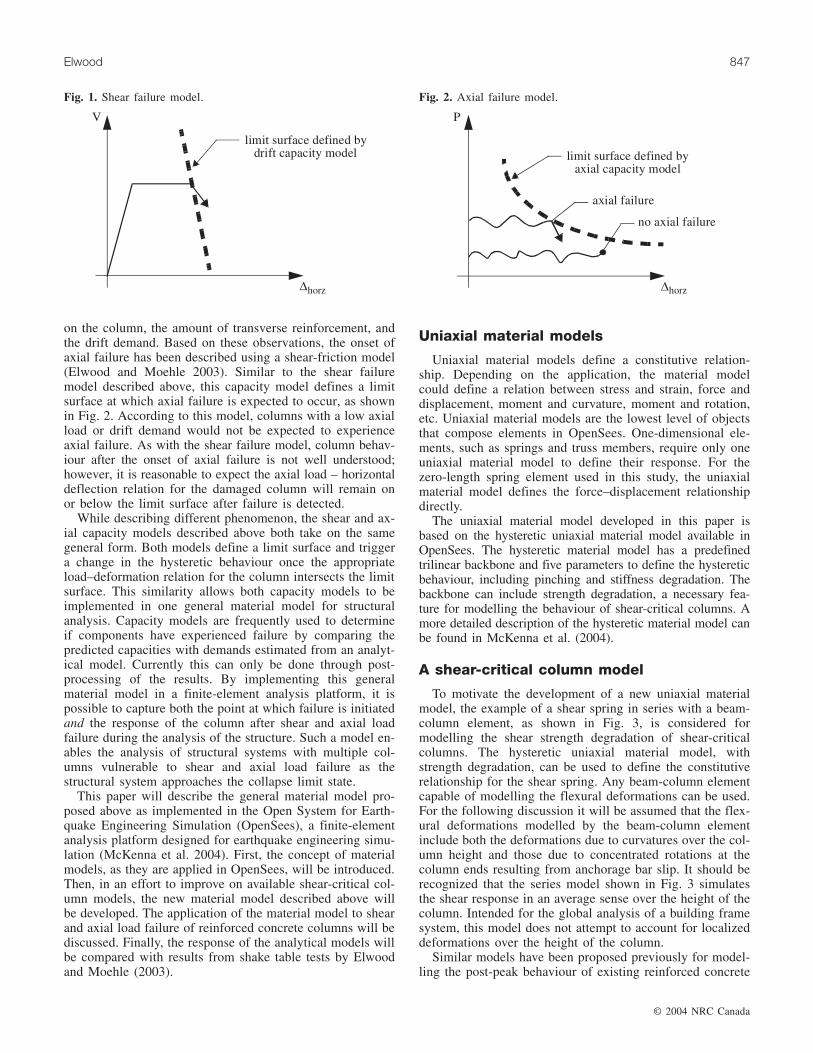
on the column, the amount of transverse reinforcement, andthe drift demand. Based on these observations, the onset ofaxial failure has been described using a shear-friction model(Elwood and Moehle 2003). Similar to the shear failuremodel described above, this capacity model defines a limitsurface at which axial failure is expected to occur, as shownin Fig. 2. According to this model, columns with a low axialload or drift demand would not be expected to experienceaxial failure. As with the shear failure model, column behav-iour after the onset of axial failure is not well understood;however, it is reasonable to expect the axial load – horizontaldeflection relation for the damaged column will remain onor below the limit surface after failure is detected.

While describing different phenomenon, the shear and ax-ial capacity models described above both take on the samegeneral form. Both models define a limit surface and triggera change in the hysteretic behaviour once the appropriateload–deformation relation for the column intersects the limitsurface. This similarity allows both capacity models to beimplemented in one general material model for structuralanalysis. Capacity models are frequently used to determineif components have experienced failure by comparing thepredicted capacities with demands estimated from an analyt-ical model. Currently this can only be done through post-processing of the results. By implementing this generalmaterial model in a finite-element analysis platform, it ispossible to capture both the point at which failure is initiatedand the response of the column after shear and axial loadfailure during the analysis of the structure. Such a model en-ables the analysis of structural systems with multiple col-umns vulnerable to shear and axial load failure as thestructural system approaches the collapse limit state.

This paper will describe the general material model pro-posed above as implemented in the Open System for Earth-quake Engineering Simulation (OpenSees), a finite-elementanalysis platform designed for earthquake engineering simu-lation (McKenna et al. 2004). First, the concept of materialmodels, as they are applied in OpenSees, will be introduced.Then, in an effort to improve on available shear-critical col-umn models, the new material model described above willbe developed. The application of the material model to shearand axial load failure of reinforced concrete columns will bediscussed. Finally, the response of the analytical models willbe compared with results from shake table tests by Elwoodand Moehle (2003).

Uniaxial material models

Uniaxial material models define a constitutive relation-ship. Depending on the application, the material modelcould define a relation between stress and strain, force anddisplacement, moment and curvature, moment and rotation,etc. Uniaxial material models are the lowest level of objectsthat compose elements in OpenSees. One-dimensional ele-ments, such as springs and truss members, require only oneuniaxial material model to define their response. For thezero-length spring element used in this study, the uniaxialmaterial model defines the force–displacement relationshipdirectly.

The uniaxial material model developed in this paper isbased on the hysteretic uniaxial material model available inOpenSees. The hysteretic material model has a predefinedtrilinear backbone and five parameters to define the hystereticbehaviour, including pinching and stiffness degradation. Thebackbone can include strength degradation, a necessary fea-ture for modelling the behaviour of shear-critical columns. Amore detailed description of the hysteretic material model canbe found in McKenna et al. (2004).

A shear-critical column model

To motivate the development of a new uniaxial materialmodel, the example of a shear spring in series with a beam-column element, as shown in Fig. 3, is considered formodelling the shear strength degradation of shear-criticalcolumns. The hysteretic uniaxial material model, withstrength degradation, can be used to define the constitutiverelationship for the shear spring. Any beam-column elementcapable of modelling the flexural deformations can be used.For the following discussion it will be assumed that the flex-ural deformations modelled by the beam-column elementinclude both the deformations due to curvatures over the col-umn height and those due to concentrated rotations at thecolumn ends resulting from anchorage bar slip. It should berecognized that the series model shown in Fig. 3 simulatesthe shear response in an average sense over the height of thecolumn. Intended for the global analysis of a building framesystem, this model does not attempt to account for localizeddeformations over the height of the column.

Similar models have been proposed previously for model-ling the post-peak behaviour of existing reinforced concrete

© 2004 NRC Canada

Elwood 847

Fig. 1. Shear failure model. Fig. 2. Axial failure model.

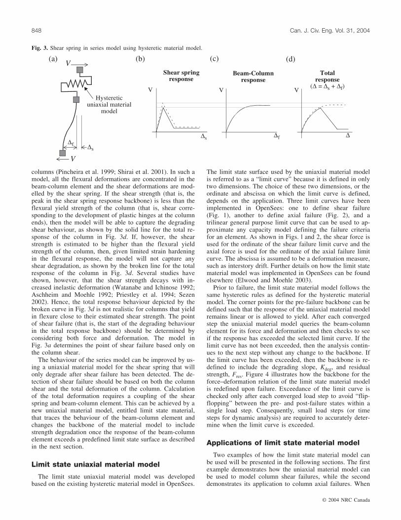
columns (Pincheira et al. 1999; Shirai et al. 2001). In such amodel, all the flexural deformations are concentrated in thebeam-column element and the shear deformations are mod-elled by the shear spring. If the shear strength (that is, thepeak in the shear spring response backbone) is less than theflexural yield strength of the column (that is, shear corre-sponding to the development of plastic hinges at the columnends), then the model will be able to capture the degradingshear behaviour, as shown by the solid line for the total re-sponse of the column in Fig. 3d. If, however, the shearstrength is estimated to be higher than the flexural yieldstrength of the column, then, given limited strain hardeningin the flexural response, the model will not capture anyshear degradation, as shown by the broken line for the totalresponse of the column in Fig. 3d. Several studies haveshown, however, that the shear strength decays with in-creased inelastic deformation (Watanabe and Ichinose 1992;Aschheim and Moehle 1992; Priestley et al. 1994; Sezen2002). Hence, the total response behaviour depicted by thebroken curve in Fig. 3d is not realistic for columns that yieldin flexure close to their estimated shear strength. The pointof shear failure (that is, the start of the degrading behaviourin the total response backbone) should be determined byconsidering both force and deformation. The model inFig. 3a determines the point of shear failure based only onthe column shear.

The behaviour of the series model can be improved by us-ing a uniaxial material model for the shear spring that willonly degrade after shear failure has been detected. The de-tection of shear failure should be based on both the columnshear and the total deformation of the column. Calculationof the total deformation requires a coupling of the shearspring and beam-column element. This can be achieved by anew uniaxial material model, entitled limit state material,that traces the behaviour of the beam-column element andchanges the backbone of the material model to includestrength degradation once the response of the beam-columnelement exceeds a predefined limit state surface as describedin the next section.

Limit state uniaxial material model

The limit state uniaxial material model was developedbased on the existing hysteretic material model in OpenSees.

The limit state surface used by the uniaxial material modelis referred to as a “limit curve” because it is defined in onlytwo dimensions. The choice of these two dimensions, or theordinate and abscissa on which the limit curve is defined,depends on the application. Three limit curves have beenimplemented in OpenSees: one to define shear failure(Fig. 1), another to define axial failure (Fig. 2), and atrilinear general purpose limit curve that can be used to ap-proximate any capacity model defining the failure criteriafor an element. As shown in Figs. l and 2, the shear force isused for the ordinate of the shear failure limit curve and theaxial force is used for the ordinate of the axial failure limitcurve. The abscissa is assumed to be a deformation measure,such as interstory drift. Further details on how the limit statematerial model was implemented in OpenSees can be foundelsewhere (Elwood and Moehle 2003).

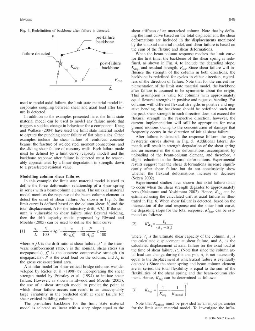
Prior to failure, the limit state material model follows thesame hysteretic rules as defined for the hysteretic materialmodel. The corner points for the pre-failure backbone can bedefined such that the response of the uniaxial material modelremains linear or is allowed to yield. After each convergedstep the uniaxial material model queries the beam-columnelement for its force and deformation and then checks to seeif the response has exceeded the selected limit curve. If thelimit curve has not been exceeded, then the analysis contin-ues to the next step without any change to the backbone. Ifthe limit curve has been exceeded, then the backbone is re-defined to include the degrading slope, Kdeg, and residualstrength, Fres. Figure 4 illustrates how the backbone for theforce–deformation relation of the limit state material modelis redefined upon failure. Exceedance of the limit curve ischecked only after each converged load step to avoid “flip-flopping” between the pre- and post-failure states within asingle load step. Consequently, small load steps (or timesteps for dynamic analysis) are required to accurately deter-mine when the limit curve is exceeded.

Applications of limit state material model

Two examples of how the limit state material model canbe used will be presented in the following sections. The firstexample demonstrates how the uniaxial material model canbe used to model column shear failures, while the seconddemonstrates its application to column axial failures. When

© 2004 NRC Canada

848 Can. J. Civ. Eng. Vol. 31, 2004

Fig. 3. Shear spring in series model using hysteretic material model.

used to model axial failure, the limit state material model in-corporates coupling between shear and axial load after fail-ure is detected.

In addition to the examples presented here, the limit statematerial model can be used to model any failure mode thattriggers a sudden change in behaviour for a component. Kangand Wallace (2004) have used the limit state material modelto capture the punching shear failure of flat plate slabs. Otherexamples include the shear failure of reinforced concretebeams, the fracture of welded steel moment connections, andthe sliding shear failure of masonry walls. Each failure modemust be defined by a limit curve (capacity model) and thebackbone response after failure is detected must be reason-ably approximated by a linear degradation in strength, downto a preselected residual value.

Modelling column shear failuresIn this example the limit state material model is used to

define the force–deformation relationship of a shear springin series with a beam-column element. The uniaxial materialmodel monitors the response of the beam-column element todetect the onset of shear failure. As shown in Fig. 5, thelimit curve is defined based on the column shear, V, and thetotal displacement, ∆ (or the interstory drift, ∆/L). If the col-umn is vulnerable to shear failure after flexural yielding,then the drift capacity model proposed by Elwood andMoehle (2005) can be used to define the limit curve

[1]∆s

c g cLv

f

PA f

= + ′′−′−

′≥3

1004

140

140

1100

ρ

where ∆ s/L is the drift ratio at shear failure, ρ′ ′ is the trans-verse reinforcement ratio, ν is the nominal shear stress (inmegapascals), fc′ is the concrete compressive strength (inmegapascals), P is the axial load on the column, and Ag isthe gross cross-sectional area.

A similar model for shear-critical bridge columns was de-veloped by Ricles et al. (1998) by incorporating the shearstrength model by Priestley et al. (1994) to initiate shearfailure. However, as shown in Elwood and Moehle (2005),the use of a shear strength model to predict the point atwhich shear failure occurs can result in an unacceptablylarge variability in the predicted drift at shear failure forshear-critical building columns.

The pre-failure backbone for the limit state materialmodel is selected as linear with a steep slope equal to the

shear stiffness of an uncracked column. Note that by defin-ing the limit curve based on the total displacement, the sheardeformations are included in the displacements monitoredby the uniaxial material model, and shear failure is based onthe sum of the flexure and shear deformations.

When the beam-column response reaches the limit curvefor the first time, the backbone of the shear spring is rede-fined, as shown in Fig. 4, to include the degrading slope,Kdeg, and residual strength, Fres. Since shear failure will in-fluence the strength of the column in both directions, thebackbone is redefined for cycles in either direction, regard-less of the direction of failure. Note that for the current im-plementation of the limit state material model, the backboneafter failure is assumed to be symmetric about the origin.This assumption is valid for columns with approximatelyequal flexural strengths in positive and negative bending. Forcolumns with different flexural strengths in positive and neg-ative bending, the backbone should be redefined such thatthe peak shear strength in each direction does not exceed theflexural strength in the respective direction; however, thecurrent implementation will still be appropriate for mostground motions owing to the concentration of damage thatfrequently occurs in the direction of initial shear failure.

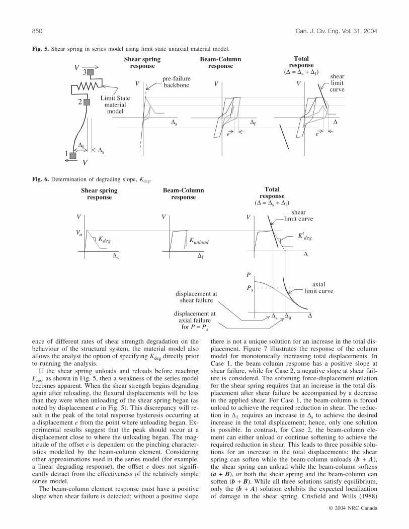
After failure is detected, the response follows the grayhysteretic curves shown in Fig. 5. Additional lateral de-mands will result in strength degradation of the shear springand an increase in the shear deformations, accompanied byunloading of the beam-column element, and therefore, aslight reduction in the flexural deformations. Experimentalresults suggest that the shear deformations increase signifi-cantly after shear failure but do not conclusively showwhether the flexural deformations increase or decrease(Sezen 2002).

Experimental studies have shown that axial failure tendsto occur when the shear strength degrades to approximatelyzero (Nakamura and Yoshimura 2002). Hence, Kdeg can beestimated using the calculated drift at axial failure as illus-trated in Fig. 6. When shear failure is detected, based on theintersection of the total response and the shear limit curve,the degrading slope for the total response, K deg

t , can be esti-mated as follows:

[2] KV

degt u

a s

=−( )∆ ∆

where Vu is the ultimate shear capacity of the column, ∆ s isthe calculated displacement at shear failure, and ∆a is thecalculated displacement at axial failure for the axial load atthe time of shear failure, Ps. (Note that since the column ax-ial load can change during the analysis, ∆s is not necessarilyequal to the displacement at which axial failure is eventuallydetected.) Since the shear spring and beam-column elementare in series, the total flexibility is equal to the sum of theflexibilities of the shear spring and the beam-column ele-ment. Hence, Kdeg can be determined as follows:

[3] KK K

degdegt

unload

= −⎛

⎝

⎜⎜

⎞

⎠

⎟⎟

−1 1

1

Note that Kunload must be provided as an input parameterfor the limit state material model. To investigate the influ-

© 2004 NRC Canada

Elwood 849

Fig. 4. Redefinition of backbone after failure is detected.

ence of different rates of shear strength degradation on thebehaviour of the structural system, the material model alsoallows the analyst the option of specifying Kdeg directly priorto running the analysis.

If the shear spring unloads and reloads before reachingFres, as shown in Fig. 5, then a weakness of the series modelbecomes apparent. When the shear strength begins degradingagain after reloading, the flexural displacements will be lessthan they were when unloading of the shear spring began (asnoted by displacement e in Fig. 5). This discrepancy will re-sult in the peak of the total response hysteresis occurring ata displacement e from the point where unloading began. Ex-perimental results suggest that the peak should occur at adisplacement close to where the unloading began. The mag-nitude of the offset e is dependent on the pinching character-istics modelled by the beam-column element. Consideringother approximations used in the series model (for example,a linear degrading response), the offset e does not signifi-cantly detract from the effectiveness of the relatively simpleseries model.

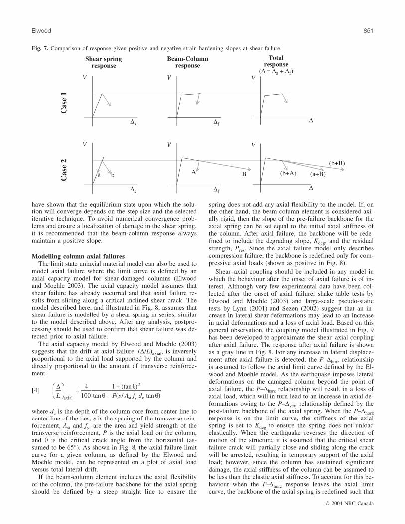
The beam-column element response must have a positiveslope when shear failure is detected; without a positive slope

there is not a unique solution for an increase in the total dis-placement. Figure 7 illustrates the response of the columnmodel for monotonically increasing total displacements. InCase 1, the beam-column response has a positive slope atshear failure, while for Case 2, a negative slope at shear fail-ure is considered. The softening force-displacement relationfor the shear spring requires that an increase in the total dis-placement after shear failure be accompanied by a decreasein the applied shear. For Case 1, the beam-column is forcedunload to achieve the required reduction in shear. The reduc-tion in ∆ f requires an increase in ∆s to achieve the desiredincrease in the total displacement; hence, only one solutionis possible. In contrast, for Case 2, the beam-column ele-ment can either unload or continue softening to achieve therequired reduction in shear. This leads to three possible solu-tions for an increase in the total displacements: the shearspring can soften while the beam-column unloads (b + A),the shear spring can unload while the beam-column softens(a + B), or both the shear spring and the beam-column cansoften (b + B). While all three solutions satisfy equilibrium,only the (b + A) solution exhibits the expected localizationof damage in the shear spring. Crisfield and Wills (1988)

© 2004 NRC Canada

850 Can. J. Civ. Eng. Vol. 31, 2004

Fig. 5. Shear spring in series model using limit state uniaxial material model.

Fig. 6. Determination of degrading slope, Kdeg.

have shown that the equilibrium state upon which the solu-tion will converge depends on the step size and the selectediterative technique. To avoid numerical convergence prob-lems and ensure a localization of damage in the shear spring,it is recommended that the beam-column response alwaysmaintain a positive slope.

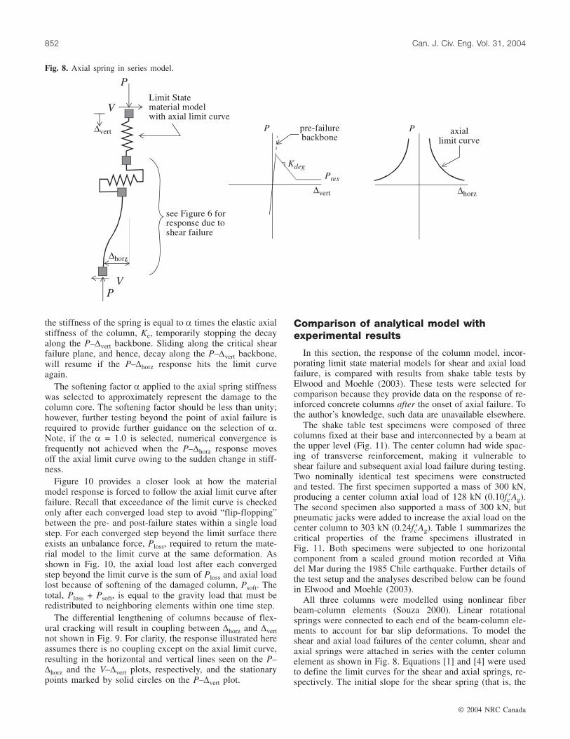
Modelling column axial failuresThe limit state uniaxial material model can also be used to

model axial failure where the limit curve is defined by anaxial capacity model for shear-damaged columns (Elwoodand Moehle 2003). The axial capacity model assumes thatshear failure has already occurred and that axial failure re-sults from sliding along a critical inclined shear crack. Themodel described here, and illustrated in Fig. 8, assumes thatshear failure is modelled by a shear spring in series, similarto the model described above. After any analysis, postpro-cessing should be used to confirm that shear failure was de-tected prior to axial failure.

The axial capacity model by Elwood and Moehle (2003)suggests that the drift at axial failure, (∆/L)axial, is inverselyproportional to the axial load supported by the column anddirectly proportional to the amount of transverse reinforce-ment

[4]∆L P s A f d

⎛⎝⎜

⎞⎠⎟ = +

+axial st yt c

4100

1 2(tan )tan ( / tan )

θθ θ

where dc is the depth of the column core from center line tocenter line of the ties, s is the spacing of the transverse rein-forcement, Ast and fyt are the area and yield strength of thetransverse reinforcement, P is the axial load on the column,and θ is the critical crack angle from the horizontal (as-sumed to be 65°). As shown in Fig. 8, the axial failure limitcurve for a given column, as defined by the Elwood andMoehle model, can be represented on a plot of axial loadversus total lateral drift.

If the beam-column element includes the axial flexibilityof the column, the pre-failure backbone for the axial springshould be defined by a steep straight line to ensure the

spring does not add any axial flexibility to the model. If, onthe other hand, the beam-column element is considered axi-ally rigid, then the slope of the pre-failure backbone for theaxial spring can be set equal to the initial axial stiffness ofthe column. After axial failure, the backbone will be rede-fined to include the degrading slope, Kdeg, and the residualstrength, Pres. Since the axial failure model only describescompression failure, the backbone is redefined only for com-pressive axial loads (shown as positive in Fig. 8).

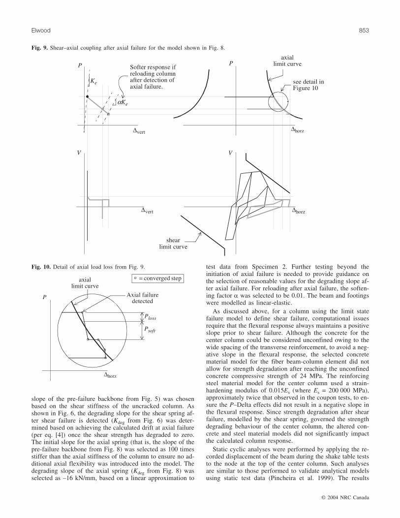
Shear–axial coupling should be included in any model inwhich the behaviour after the onset of axial failure is of in-terest. Although very few experimental data have been col-lected after the onset of axial failure, shake table tests byElwood and Moehle (2003) and large-scale pseudo-statictests by Lynn (2001) and Sezen (2002) suggest that an in-crease in lateral shear deformations may lead to an increasein axial deformations and a loss of axial load. Based on thisgeneral observation, the coupling model illustrated in Fig. 9has been developed to approximate the shear–axial couplingafter axial failure. The response after axial failure is shownas a gray line in Fig. 9. For any increase in lateral displace-ment after axial failure is detected, the P–∆horz relationshipis assumed to follow the axial limit curve defined by the El-wood and Moehle model. As the earthquake imposes lateraldeformations on the damaged column beyond the point ofaxial failure, the P–∆horz relationship will result in a loss ofaxial load, which will in turn lead to an increase in axial de-formations owing to the P–∆vert relationship defined by thepost-failure backbone of the axial spring. When the P–∆horzresponse is on the limit curve, the stiffness of the axialspring is set to Kdeg to ensure the spring does not unloadelastically. When the earthquake reverses the direction ofmotion of the structure, it is assumed that the critical shearfailure crack will partially close and sliding along the crackwill be arrested, resulting in temporary support of the axialload; however, since the column has sustained significantdamage, the axial stiffness of the column can be assumed tobe less than the elastic axial stiffness. To account for this be-haviour when the P–∆horz response leaves the axial limitcurve, the backbone of the axial spring is redefined such that

© 2004 NRC Canada

Elwood 851

Fig. 7. Comparison of response given positive and negative strain hardening slopes at shear failure.

the stiffness of the spring is equal to α times the elastic axialstiffness of the column, Ke, temporarily stopping the decayalong the P–∆vert backbone. Sliding along the critical shearfailure plane, and hence, decay along the P–∆vert backbone,will resume if the P–∆horz response hits the limit curveagain.

The softening factor α applied to the axial spring stiffnesswas selected to approximately represent the damage to thecolumn core. The softening factor should be less than unity;however, further testing beyond the point of axial failure isrequired to provide further guidance on the selection of α.Note, if the α = 1.0 is selected, numerical convergence isfrequently not achieved when the P–∆horz response movesoff the axial limit curve owing to the sudden change in stiff-ness.

Figure 10 provides a closer look at how the materialmodel response is forced to follow the axial limit curve afterfailure. Recall that exceedance of the limit curve is checkedonly after each converged load step to avoid “flip-flopping”between the pre- and post-failure states within a single loadstep. For each converged step beyond the limit surface thereexists an unbalance force, Ploss, required to return the mate-rial model to the limit curve at the same deformation. Asshown in Fig. 10, the axial load lost after each convergedstep beyond the limit curve is the sum of Ploss and axial loadlost because of softening of the damaged column, Psoft. Thetotal, Ploss + Psoft, is equal to the gravity load that must beredistributed to neighboring elements within one time step.

The differential lengthening of columns because of flex-ural cracking will result in coupling between ∆horz and ∆vertnot shown in Fig. 9. For clarity, the response illustrated hereassumes there is no coupling except on the axial limit curve,resulting in the horizontal and vertical lines seen on the P–∆horz and the V–∆vert plots, respectively, and the stationarypoints marked by solid circles on the P–∆vert plot.

Comparison of analytical model withexperimental results

In this section, the response of the column model, incor-porating limit state material models for shear and axial loadfailure, is compared with results from shake table tests byElwood and Moehle (2003). These tests were selected forcomparison because they provide data on the response of re-inforced concrete columns after the onset of axial failure. Tothe author’s knowledge, such data are unavailable elsewhere.

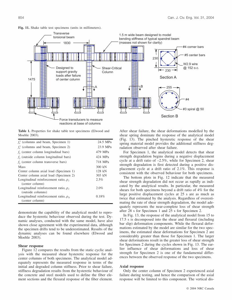
The shake table test specimens were composed of threecolumns fixed at their base and interconnected by a beam atthe upper level (Fig. 11). The center column had wide spac-ing of transverse reinforcement, making it vulnerable toshear failure and subsequent axial load failure during testing.Two nominally identical test specimens were constructedand tested. The first specimen supported a mass of 300 kN,producing a center column axial load of 128 kN (0.10fc′Ag).The second specimen also supported a mass of 300 kN, butpneumatic jacks were added to increase the axial load on thecenter column to 303 kN (0.24fc′Ag). Table 1 summarizes thecritical properties of the frame specimens illustrated inFig. 11. Both specimens were subjected to one horizontalcomponent from a scaled ground motion recorded at Viñadel Mar during the 1985 Chile earthquake. Further details ofthe test setup and the analyses described below can be foundin Elwood and Moehle (2003).

All three columns were modelled using nonlinear fiberbeam-column elements (Souza 2000). Linear rotationalsprings were connected to each end of the beam-column ele-ments to account for bar slip deformations. To model theshear and axial load failures of the center column, shear andaxial springs were attached in series with the center columnelement as shown in Fig. 8. Equations [1] and [4] were usedto define the limit curves for the shear and axial springs, re-spectively. The initial slope for the shear spring (that is, the

© 2004 NRC Canada

852 Can. J. Civ. Eng. Vol. 31, 2004

Fig. 8. Axial spring in series model.

slope of the pre-failure backbone from Fig. 5) was chosenbased on the shear stiffness of the uncracked column. Asshown in Fig. 6, the degrading slope for the shear spring af-ter shear failure is detected (Kdeg from Fig. 6) was deter-mined based on achieving the calculated drift at axial failure(per eq. [4]) once the shear strength has degraded to zero.The initial slope for the axial spring (that is, the slope of thepre-failure backbone from Fig. 8) was selected as 100 timesstiffer than the axial stiffness of the column to ensure no ad-ditional axial flexibility was introduced into the model. Thedegrading slope of the axial spring (Kdeg from Fig. 8) wasselected as –16 kN/mm, based on a linear approximation to

test data from Specimen 2. Further testing beyond theinitiation of axial failure is needed to provide guidance onthe selection of reasonable values for the degrading slope af-ter axial failure. For reloading after axial failure, the soften-ing factor α was selected to be 0.01. The beam and footingswere modelled as linear-elastic.

As discussed above, for a column using the limit statefailure model to define shear failure, computational issuesrequire that the flexural response always maintains a positiveslope prior to shear failure. Although the concrete for thecenter column could be considered unconfined owing to thewide spacing of the transverse reinforcement, to avoid a neg-ative slope in the flexural response, the selected concretematerial model for the fiber beam-column element did notallow for strength degradation after reaching the unconfinedconcrete compressive strength of 24 MPa. The reinforcingsteel material model for the center column used a strain-hardening modulus of 0.015Es (where Es = 200 000 MPa),approximately twice that observed in the coupon tests, to en-sure the P–Delta effects did not result in a negative slope inthe flexural response. Since strength degradation after shearfailure, modelled by the shear spring, governed the strengthdegrading behaviour of the center column, the altered con-crete and steel material models did not significantly impactthe calculated column response.

Static cyclic analyses were performed by applying the re-corded displacement of the beam during the shake table teststo the node at the top of the center column. Such analysesare similar to those performed to validate analytical modelsusing static test data (Pincheira et al. 1999). The results

© 2004 NRC Canada

Elwood 853

Fig. 9. Shear–axial coupling after axial failure for the model shown in Fig. 8.

Fig. 10. Detail of axial load loss from Fig. 9.

demonstrate the capability of the analytical model to repro-duce the hysteretic behaviour observed during the test. Dy-namic analyses, conducted with the same model, have alsoshown close agreement with the experimental data, althoughthe specimen drifts tend to be underestimated. Results of thedynamic analyses can be found elsewhere (Elwood andMoehle 2003).

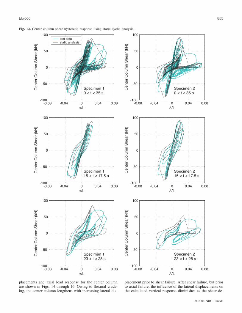
Shear responseFigure 12 compares the results from the static cyclic anal-

ysis with the measured shear hysteretic response for thecenter columns of both specimens. The analytical model ad-equately represents the measured response in terms of theinitial and degraded column stiffness. Prior to shear failure,stiffness degradation results from the hysteretic behaviour ofthe concrete and steel models used to define the fiber ele-ment sections and the flexural response of the fiber element.

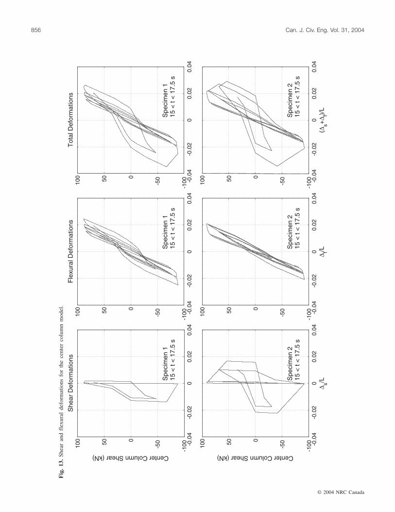
After shear failure, the shear deformations modelled by theshear spring dominate the response of the analytical model(Fig. 13). The pinched hysteretic response of the shearspring material model provides the additional stiffness deg-radation observed after shear failure.

For Specimen 1, the analytical model detects that shearstrength degradation begins during a negative displacementcycle at a drift ratio of –2.5%, while for Specimen 2, shearstrength degradation is first detected during a positive dis-placement cycle at a drift ratio of 2.1%. This response isconsistent with the observed behaviour for both specimens.

The bottom plots in Fig. 12 indicate that the measuredshear strength degradation did not occur as rapidly as indi-cated by the analytical results. In particular, the measuredshears for both specimens beyond a drift ratio of 4% for thelarge positive displacement cycles at 25 s are as much astwice that estimated by the analysis. Regardless of overesti-mating the rate of shear strength degradation, the model ade-quately represents the near-complete loss of shear strengthafter 28 s for Specimen 1 and 25 s for Specimen 2.

In Fig. 13, the response of the analytical model from 15 to17.5 s is decomposed into the shear and flexural (includingbar slip) deformation components. While the flexural defor-mations estimated by the model are similar for the two spec-imens, the estimated shear deformations for Specimen 2 areconsiderably greater than those for Specimen 1. The largershear deformations result in the greater loss of shear strengthfor Specimen 2 during the cycles shown in Fig. 13. The ear-lier influence of shear deformations and loss of shearstrength for Specimen 2 is one of the fundamental differ-ences between the observed response of the two specimens.

Axial responseOnly the center column of Specimen 2 experienced axial

failure during testing, and hence the comparison of the axialresponse will be limited to this component. The vertical dis-

© 2004 NRC Canada

854 Can. J. Civ. Eng. Vol. 31, 2004

Fig. 11. Shake table test specimens (units in millimeters).

fc′ (columns and beam, Specimen 1) 24.5 MPa

fc′ (columns and beam, Specimen 2) 23.9 MPa

fy (center column longitudinal bars) 479 MPa

fy (outside column longitudinal bars) 424 MPa

fy (center column transverse bars) 718 MPa

Mass 300 kNCenter column axial load (Specimen 1) 128 kNCenter column axial load (Specimen 2) 303 kNLongitudinal reinforcement ratio, ρl

(center column)2.5%

Longitudinal reinforcement ratio, ρl

(outside columns)2.0%

Longitudinal reinforcement ratio, ρh

(center column)0.18%

Table 1. Properties for shake table test specimens (Elwood andMoehle 2003).

placements and axial load response for the center columnare shown in Figs. 14 through 16. Owing to flexural crack-ing, the center column lengthens with increasing lateral dis-

placement prior to shear failure. After shear failure, but priorto axial failure, the influence of the lateral displacements onthe calculated vertical response diminishes as the shear de-

© 2004 NRC Canada

Elwood 855

Fig. 12. Center column shear hysteretic response using static cyclic analysis.

© 2004 NRC Canada

856 Can. J. Civ. Eng. Vol. 31, 2004

Fig

.13

.S

hear

and

flex

ural

defo

rmat

ions

for

the

cent

erco

lum

nm

odel

.

© 2004 NRC Canada

Elwood 857

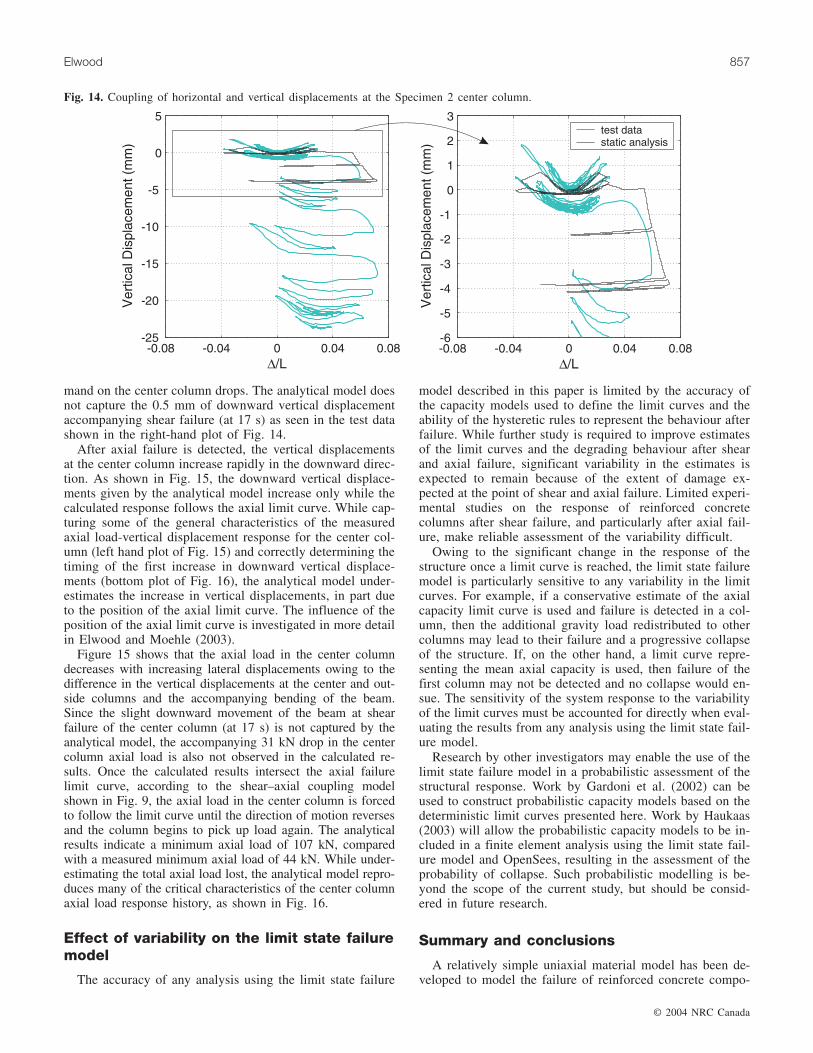
mand on the center column drops. The analytical model doesnot capture the 0.5 mm of downward vertical displacementaccompanying shear failure (at 17 s) as seen in the test datashown in the right-hand plot of Fig. 14.

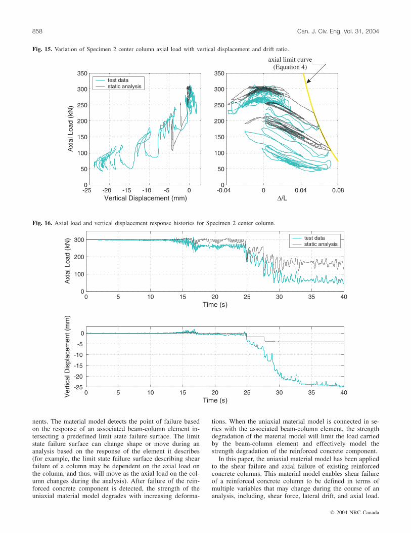
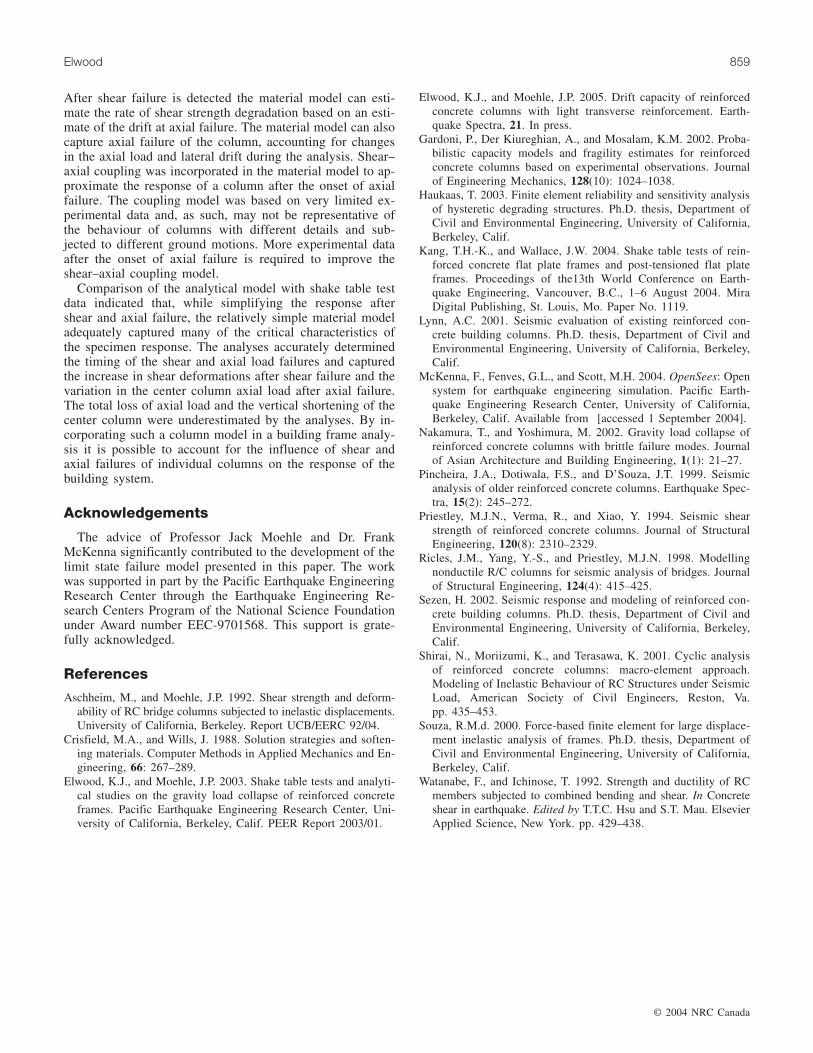
After axial failure is detected, the vertical displacementsat the center column increase rapidly in the downward direc-tion. As shown in Fig. 15, the downward vertical displace-ments given by the analytical model increase only while thecalculated response follows the axial limit curve. While cap-turing some of the general characteristics of the measuredaxial load-vertical displacement response for the center col-umn (left hand plot of Fig. 15) and correctly determining thetiming of the first increase in downward vertical displace-ments (bottom plot of Fig. 16), the analytical model under-estimates the increase in vertical displacements, in part dueto the position of the axial limit curve. The influence of theposition of the axial limit curve is investigated in more detailin Elwood and Moehle (2003).

Figure 15 shows that the axial load in the center columndecreases with increasing lateral displacements owing to thedifference in the vertical displacements at the center and out-side columns and the accompanying bending of the beam.Since the slight downward movement of the beam at shearfailure of the center column (at 17 s) is not captured by theanalytical model, the accompanying 31 kN drop in the centercolumn axial load is also not observed in the calculated re-sults. Once the calculated results intersect the axial failurelimit curve, according to the shear–axial coupling modelshown in Fig. 9, the axial load in the center column is forcedto follow the limit curve until the direction of motion reversesand the column begins to pick up load again. The analyticalresults indicate a minimum axial load of 107 kN, comparedwith a measured minimum axial load of 44 kN. While under-estimating the total axial load lost, the analytical model repro-duces many of the critical characteristics of the center columnaxial load response history, as shown in Fig. 16.

Effect of variability on the limit state failuremodel

The accuracy of any analysis using the limit state failure

model described in this paper is limited by the accuracy ofthe capacity models used to define the limit curves and theability of the hysteretic rules to represent the behaviour afterfailure. While further study is required to improve estimatesof the limit curves and the degrading behaviour after shearand axial failure, significant variability in the estimates isexpected to remain because of the extent of damage ex-pected at the point of shear and axial failure. Limited experi-mental studies on the response of reinforced concretecolumns after shear failure, and particularly after axial fail-ure, make reliable assessment of the variability difficult.

Owing to the significant change in the response of thestructure once a limit curve is reached, the limit state failuremodel is particularly sensitive to any variability in the limitcurves. For example, if a conservative estimate of the axialcapacity limit curve is used and failure is detected in a col-umn, then the additional gravity load redistributed to othercolumns may lead to their failure and a progressive collapseof the structure. If, on the other hand, a limit curve repre-senting the mean axial capacity is used, then failure of thefirst column may not be detected and no collapse would en-sue. The sensitivity of the system response to the variabilityof the limit curves must be accounted for directly when eval-uating the results from any analysis using the limit state fail-ure model.

Research by other investigators may enable the use of thelimit state failure model in a probabilistic assessment of thestructural response. Work by Gardoni et al. (2002) can beused to construct probabilistic capacity models based on thedeterministic limit curves presented here. Work by Haukaas(2003) will allow the probabilistic capacity models to be in-cluded in a finite element analysis using the limit state fail-ure model and OpenSees, resulting in the assessment of theprobability of collapse. Such probabilistic modelling is be-yond the scope of the current study, but should be consid-ered in future research.

Summary and conclusions

A relatively simple uniaxial material model has been de-veloped to model the failure of reinforced concrete compo-

Fig. 14. Coupling of horizontal and vertical displacements at the Specimen 2 center column.

nents. The material model detects the point of failure basedon the response of an associated beam-column element in-tersecting a predefined limit state failure surface. The limitstate failure surface can change shape or move during ananalysis based on the response of the element it describes(for example, the limit state failure surface describing shearfailure of a column may be dependent on the axial load onthe column, and thus, will move as the axial load on the col-umn changes during the analysis). After failure of the rein-forced concrete component is detected, the strength of theuniaxial material model degrades with increasing deforma-

tions. When the uniaxial material model is connected in se-ries with the associated beam-column element, the strengthdegradation of the material model will limit the load carriedby the beam-column element and effectively model thestrength degradation of the reinforced concrete component.

In this paper, the uniaxial material model has been appliedto the shear failure and axial failure of existing reinforcedconcrete columns. This material model enables shear failureof a reinforced concrete column to be defined in terms ofmultiple variables that may change during the course of ananalysis, including, shear force, lateral drift, and axial load.

© 2004 NRC Canada

858 Can. J. Civ. Eng. Vol. 31, 2004

Fig. 15. Variation of Specimen 2 center column axial load with vertical displacement and drift ratio.

Fig. 16. Axial load and vertical displacement response histories for Specimen 2 center column.

After shear failure is detected the material model can esti-mate the rate of shear strength degradation based on an esti-mate of the drift at axial failure. The material model can alsocapture axial failure of the column, accounting for changesin the axial load and lateral drift during the analysis. Shear–axial coupling was incorporated in the material model to ap-proximate the response of a column after the onset of axialfailure. The coupling model was based on very limited ex-perimental data and, as such, may not be representative ofthe behaviour of columns with different details and sub-jected to different ground motions. More experimental dataafter the onset of axial failure is required to improve theshear–axial coupling model.

Comparison of the analytical model with shake table testdata indicated that, while simplifying the response aftershear and axial failure, the relatively simple material modeladequately captured many of the critical characteristics ofthe specimen response. The analyses accurately determinedthe timing of the shear and axial load failures and capturedthe increase in shear deformations after shear failure and thevariation in the center column axial load after axial failure.The total loss of axial load and the vertical shortening of thecenter column were underestimated by the analyses. By in-corporating such a column model in a building frame analy-sis it is possible to account for the influence of shear andaxial failures of individual columns on the response of thebuilding system.

Acknowledgements

The advice of Professor Jack Moehle and Dr. FrankMcKenna significantly contributed to the development of thelimit state failure model presented in this paper. The workwas supported in part by the Pacific Earthquake EngineeringResearch Center through the Earthquake Engineering Re-search Centers Program of the National Science Foundationunder Award number EEC-9701568. This support is grate-fully acknowledged.

References

Aschheim, M., and Moehle, J.P. 1992. Shear strength and deform-ability of RC bridge columns subjected to inelastic displacements.University of California, Berkeley. Report UCB/EERC 92/04.

Crisfield, M.A., and Wills, J. 1988. Solution strategies and soften-ing materials. Computer Methods in Applied Mechanics and En-gineering, 66: 267–289.

Elwood, K.J., and Moehle, J.P. 2003. Shake table tests and analyti-cal studies on the gravity load collapse of reinforced concreteframes. Pacific Earthquake Engineering Research Center, Uni-versity of California, Berkeley, Calif. PEER Report 2003/01.

Elwood, K.J., and Moehle, J.P. 2005. Drift capacity of reinforcedconcrete columns with light transverse reinforcement. Earth-quake Spectra, 21. In press.

Gardoni, P., Der Kiureghian, A., and Mosalam, K.M. 2002. Proba-bilistic capacity models and fragility estimates for reinforcedconcrete columns based on experimental observations. Journalof Engineering Mechanics, 128(10): 1024–1038.

Haukaas, T. 2003. Finite element reliability and sensitivity analysisof hysteretic degrading structures. Ph.D. thesis, Department ofCivil and Environmental Engineering, University of California,Berkeley, Calif.

Kang, T.H.-K., and Wallace, J.W. 2004. Shake table tests of rein-forced concrete flat plate frames and post-tensioned flat plateframes. Proceedings of the13th World Conference on Earth-quake Engineering, Vancouver, B.C., 1–6 August 2004. MiraDigital Publishing, St. Louis, Mo. Paper No. 1119.

Lynn, A.C. 2001. Seismic evaluation of existing reinforced con-crete building columns. Ph.D. thesis, Department of Civil andEnvironmental Engineering, University of California, Berkeley,Calif.

McKenna, F., Fenves, G.L., and Scott, M.H. 2004. OpenSees: Opensystem for earthquake engineering simulation. Pacific Earth-quake Engineering Research Center, University of California,Berkeley, Calif. Available from [accessed 1 September 2004].

Nakamura, T., and Yoshimura, M. 2002. Gravity load collapse ofreinforced concrete columns with brittle failure modes. Journalof Asian Architecture and Building Engineering, 1(1): 21–27.

Pincheira, J.A., Dotiwala, F.S., and D’Souza, J.T. 1999. Seismicanalysis of older reinforced concrete columns. Earthquake Spec-tra, 15(2): 245–272.

Priestley, M.J.N., Verma, R., and Xiao, Y. 1994. Seismic shearstrength of reinforced concrete columns. Journal of StructuralEngineering, 120(8): 2310–2329.

Ricles, J.M., Yang, Y.-S., and Priestley, M.J.N. 1998. Modellingnonductile R/C columns for seismic analysis of bridges. Journalof Structural Engineering, 124(4): 415–425.

Sezen, H. 2002. Seismic response and modeling of reinforced con-crete building columns. Ph.D. thesis, Department of Civil andEnvironmental Engineering, University of California, Berkeley,Calif.

Shirai, N., Moriizumi, K., and Terasawa, K. 2001. Cyclic analysisof reinforced concrete columns: macro-element approach.Modeling of Inelastic Behaviour of RC Structures under SeismicLoad, American Society of Civil Engineers, Reston, Va.pp. 435–453.

Souza, R.M.d. 2000. Force-based finite element for large displace-ment inelastic analysis of frames. Ph.D. thesis, Department ofCivil and Environmental Engineering, University of California,Berkeley, Calif.

Watanabe, F., and Ichinose, T. 1992. Strength and ductility of RCmembers subjected to combined bending and shear. In Concreteshear in earthquake. Edited by T.T.C. Hsu and S.T. Mau. ElsevierApplied Science, New York. pp. 429–438.

© 2004 NRC Canada

Elwood 859