Embed Size (px)
Citation preview
Modelling and Optimization of Compact Sub-sea SeparatorsGas-Liquid separation
Fahad Matovu
Chemical Engineering
Supervisor: Johannes Jäschke, IKPCo-supervisor: Sigurd Skogestad, IKP
Department of Chemical Engineering
Submission date: June 2015
Norwegian University of Science and Technology

Norwegian University of Science andTechnology
NTNU
Department of Chemical Engineering
Modelling and Optimization ofCompact Sub-sea Separators
Master’s Thesisby
Fahad Matovu
Supervisor: Associate Prof. Johannes Jäschke
Co-supervisor: Prof.Sigurd Skogestad
Trondheim, June 9, 2015
i
Abstract
This Master thesis focuses on Modelling and Optimization of Compact sub-sea separa-
tors using a given separation system. The separation system consists of three separation
units: a gravity separator, a deliquidizer and a degasser.
The steady state models developed have been aimed at predicting phase separation in
the separator units. The models in addition predict stream outlet phase fractions and
flow rates based on known inlet conditions and separator geometry.
Model simulations have been performed in Matlab and results have shown trends that
are consistent with theoretical expectations. They have in some cases for the deliq-
uidizer been compared to experimental data and close agreement has been observed.
However, in other cases, validation of simulation results has not been possible due to
lack of experimental data but the results are thought to be theoretically reasonable.
Optimization on the system has been carried out aimed at maximizing the phase frac-
tions of the streams to the compressor and pump respectively. Results have shown an
average of less than 5% of dispersed phase in a continuous phase in exit streams.
ii
Preface
This thesis is written as the final work of the Master’s of Science in Chemical Engineer-
ing at the Norwegian University of Science and Technology (NTNU), 2015.
I would like to extend my sincere thanks to my supervisors Assoc.Prof Johannes Jaschke
and Prof. Sigurd Skogestad for their technical assistance, support and guidance in this
project work.
I would also like to thank Tamal Das for his assistance during the closing stages of this
work.
Thank you all.
Declaration of Compliance:I,Fahad Matovu, hereby declare that this is an independent work according to the exam
regulations of the Norwegian University of Science and Technology (NTNU).
Place and date:
Trondheim, Norway;
June 9, 2015
CONTENTS iii
ContentsAbstract . . . . . . . . . . . . . . . . . . . . . . . . . . . . . . . . . . . . . i
Preface . . . . . . . . . . . . . . . . . . . . . . . . . . . . . . . . . . . . . ii
Contents iii
List of Figures vi
List of Tables vii
1 Introduction 11.1 Overview . . . . . . . . . . . . . . . . . . . . . . . . . . . . . . . . . 1
1.2 Motivation for compact separation technology . . . . . . . . . . . . . . 2
1.3 Challenges of compact separation technology . . . . . . . . . . . . . . 3
1.4 Objectives of this work . . . . . . . . . . . . . . . . . . . . . . . . . . 3
2 Background on Compact Separation Systems 52.1 Literature review . . . . . . . . . . . . . . . . . . . . . . . . . . . . . 5
2.2 Compact separation system by Ellingsen . . . . . . . . . . . . . . . . . 8
2.3 Gravity separators . . . . . . . . . . . . . . . . . . . . . . . . . . . . . 10
2.4 Deliquidizer . . . . . . . . . . . . . . . . . . . . . . . . . . . . . . . . 11
2.5 Degasser . . . . . . . . . . . . . . . . . . . . . . . . . . . . . . . . . . 13
3 Modelling of Compact Separation System Units 163.1 Modelling of the gravity separator . . . . . . . . . . . . . . . . . . . . 16
3.1.1 Entrainment in feed pipe . . . . . . . . . . . . . . . . . . . . . 18
3.1.2 Droplet sizes and distributions . . . . . . . . . . . . . . . . . . 19
3.1.3 Separation in gas gravity section . . . . . . . . . . . . . . . . . 22
3.1.4 Gas and liquid volume fractions of exit streams . . . . . . . . . 24
3.2 Modelling of the Deliquidizer . . . . . . . . . . . . . . . . . . . . . . 27
3.2.1 Cyclonic separation in the deliquidizer . . . . . . . . . . . . . . 29
3.3 Modelling of the Degasser . . . . . . . . . . . . . . . . . . . . . . . . 37
CONTENTS iv
3.3.1 Cyclonic separation in the degasser . . . . . . . . . . . . . . . 38
4 Optimization 434.1 Problem formulation . . . . . . . . . . . . . . . . . . . . . . . . . . . 43
4.2 Objective function . . . . . . . . . . . . . . . . . . . . . . . . . . . . . 45
4.3 Constraints . . . . . . . . . . . . . . . . . . . . . . . . . . . . . . . . 46
4.4 Optimization cases . . . . . . . . . . . . . . . . . . . . . . . . . . . . 47
4.5 Sensitivity analysis . . . . . . . . . . . . . . . . . . . . . . . . . . . . 47
5 Results and discussion 495.1 Model results . . . . . . . . . . . . . . . . . . . . . . . . . . . . . . . 50
5.1.1 Gravity separator . . . . . . . . . . . . . . . . . . . . . . . . . 50
5.1.2 Deliquidizer . . . . . . . . . . . . . . . . . . . . . . . . . . . . 52
5.1.3 Degasser . . . . . . . . . . . . . . . . . . . . . . . . . . . . . 54
5.1.4 Performance of the combined models . . . . . . . . . . . . . . 56
5.2 Optimization results . . . . . . . . . . . . . . . . . . . . . . . . . . . . 58
5.2.1 Results of optimization . . . . . . . . . . . . . . . . . . . . . . 58
5.2.2 Optimal performance . . . . . . . . . . . . . . . . . . . . . . . 59
5.2.3 Sensitivity analysis . . . . . . . . . . . . . . . . . . . . . . . . 61
6 Conclusion and Future work 626.1 Conclusion . . . . . . . . . . . . . . . . . . . . . . . . . . . . . . . . 62
6.2 Future work . . . . . . . . . . . . . . . . . . . . . . . . . . . . . . . . 62
Bibliography 64
A Appendix 68A.1 Matlab model codes . . . . . . . . . . . . . . . . . . . . . . . . . . . . 68
A.1.1 par_css.m . . . . . . . . . . . . . . . . . . . . . . . . . . . . . 68
A.1.2 mod_grav.m . . . . . . . . . . . . . . . . . . . . . . . . . . . . 68
A.1.3 mod_deliq.m . . . . . . . . . . . . . . . . . . . . . . . . . . . 72
A.1.4 mod_degas.m . . . . . . . . . . . . . . . . . . . . . . . . . . . 75
A.1.5 mod_combined.m . . . . . . . . . . . . . . . . . . . . . . . . 77
CONTENTS v
A.2 Matlab optimization codes . . . . . . . . . . . . . . . . . . . . . . . . 78
A.2.1 optim.m . . . . . . . . . . . . . . . . . . . . . . . . . . . . . . 78
A.2.2 objfnc.m . . . . . . . . . . . . . . . . . . . . . . . . . . . . . 79
A.2.3 confun.m . . . . . . . . . . . . . . . . . . . . . . . . . . . . . 80
LIST OF FIGURES vi
List of Figures2.1 Compact separation system by Ellingsen . . . . . . . . . . . . . . . . . 9
2.2 Vertical gas liquid separator . . . . . . . . . . . . . . . . . . . . . . . . 11
2.3 Typical inline deliquidizer . . . . . . . . . . . . . . . . . . . . . . . . 12
2.4 BP ETAP deliquidizer installed on a platform in the North sea . . . . . 13
2.5 Typical inline degasser . . . . . . . . . . . . . . . . . . . . . . . . . . 14
2.6 Degasser installed at the test site and off-shore on Statfjord-B platform . 15
3.1 Nomenclature of gravity separator for modelling . . . . . . . . . . . . . 16
3.2 Normalized and Cumulative volume distributions of entrained liquid . . 22
3.3 Nomenclature of deliquidizer for modelling . . . . . . . . . . . . . . . 27
3.4 Trajectory of droplet experiencing a centrifugal force . . . . . . . . . . 30
3.5 Theoretical cross sectional view of the critical droplet entrance position
rl for separation . . . . . . . . . . . . . . . . . . . . . . . . . . . . . . 32
3.6 Nomenclature of degasser for modelling . . . . . . . . . . . . . . . . . 37
3.7 Theoretical cross-sectional view of “critical bubble entrance position rl”
for separation . . . . . . . . . . . . . . . . . . . . . . . . . . . . . . . 41
4.1 Nomenclature of compact separation system for optimization . . . . . . 44
5.1 Gravity separator performance for Inlet stream gas fractions f=0.7 & 0.5 51
5.2 Deliquidizer performance-Inlet gas fraction f=0.85, Split fractions (top
stream) F=0.85 & 0.7 . . . . . . . . . . . . . . . . . . . . . . . . . . . 53
5.3 Degasser performance-Inlet gas fraction f=0.15, Split fractions (top
stream) F=0.2 & 0.4 . . . . . . . . . . . . . . . . . . . . . . . . . . . . 55
LIST OF TABLES vii
List of Tables3.1 Description of variables for gravity separator modelling . . . . . . . . . 17
3.2 Description of variables for the Entrainment correlation . . . . . . . . . 19
3.3 Description of variables for deliquidizer modelling . . . . . . . . . . . 28
3.4 Description of variables for degasser modelling . . . . . . . . . . . . . 37
4.1 Optimization cases . . . . . . . . . . . . . . . . . . . . . . . . . . . . 47
5.1 Parameters used to obtain model results . . . . . . . . . . . . . . . . . 49
5.2 Performance of combined model-Gravity separator . . . . . . . . . . . 56
5.3 Performance of combined model-Degasser . . . . . . . . . . . . . . . . 57
5.4 Performance of combined model-Deliquidizer . . . . . . . . . . . . . . 57
5.5 Optimization settings for fmincon solver . . . . . . . . . . . . . . . . . 58
5.6 Optimization results for the 5 different cases . . . . . . . . . . . . . . . 59
5.7 Optimal performance-Gravity separator . . . . . . . . . . . . . . . . . 59
5.8 Optimal performance-Degasser . . . . . . . . . . . . . . . . . . . . . . 60
5.9 Optimal performance-Deliquidizer . . . . . . . . . . . . . . . . . . . . 60
5.10 Sensitivity analysis . . . . . . . . . . . . . . . . . . . . . . . . . . . . 61
1 INTRODUCTION 1
1 Introduction
Chapter 1 focuses on the general introduction to compact sub-sea separation systems.
The reasons behind the emergency of the technology, the motivation and challenges
involved, and the objectives of this work.
In chapter 2, a literature review about compact separation systems and the system by
Ellingsen (2007) used for this work are introduced. In addition, the functionality of the
separators and their parts is covered and some typical applications of compact separators
included.
Chapter 3 focuses on the concepts of modelling the separators and the underlying as-
sumptions.
Chapter 4 discusses optimization of the compact separation system including the prob-
lem formulation, objective function, constraints, optimization cases and a sensitivity
analysis on the optimal solution.
Simulation results of the steady state models and their discussion are presented in the
first section of Chapter 5. Optimization and sensitivity analysis results in the second
section. Performance in terms of balances on each separator are also presented in table
form for the combined separator model and optimal base-case.
The conclusion and future prospects are discussed in chapter 6. All matlab codes used
for simulation purposes are attached in the Appendix A.
1.1 Overview
The oil production industry is always faced with a challenge of separating oil well
streams into component phases that include oil, water and gas, so as to process them
into marketable products or dispose them off in a way that is environmentally friendly
(Sayda and Taylor, 2007).
1 INTRODUCTION 2
The conventional separation techniques are usually costly, involve equipment of consid-
erable size and weight thereby affecting the space and load requirements, which greatly
makes the processing facilities costly (Hamoud et al., 2009). Therefore, efforts are in
place to develop technologies for oil processing that reduce the size and weight of pro-
cess equipment in order to reduce cost and maximise effectiveness. This has led to the
emergence of compact inline separation systems.
These systems are interesting prospects as separation technologies for both top-side and
sub-sea separation. What makes them interesting is the fact that they minimize space
and weight while optimize separation efficiencies and that their application in existing
installations has potential to increase production (FMCtechnologies, 2011). The inline
technology is also reported to have played a major role in de-bottlenecking and upgrad-
ing of existing top-side facilities (Chin et al., 2003),(Hamoud et al., 2009).
In inline separators, the separation is achieved by the use of centrifugal forces that are
thousands of times greater than the force of gravity used in conventional separators
(Hamoud et al., 2009). In contrast to conventional separators where fluids are allowed
to have a few minutes of retention time under the influence of gravity, inline separators
need relatively much lesser retention times. This is because the rate of separation is
greatly increased in inline separators. The size of the separation vessels is also greatly
reduced (Hamoud et al., 2009).
1.2 Motivation for compact separation technology
The reduced size and weight of compact separation technologies are very attractive
because of limitation of space and load requirements thus reducing associated capital
costs. The reduced weight and space requirements of these systems also help to make
marginal fields commercially viable. Compact equipment can also be used in existing
installations where space is limited, for debottle-necking (FMCtechnologies, 2011).
Compact equipment can also be used for phase separation for top-side and sub-sea in-
stallations because of their reduced size and weight.
1 INTRODUCTION 3
Compact equipment are ideal for sub-sea separation and other high pressure applications
since pressure vessels can be reduced in size, or sometimes even be eliminated when
using inline separation equipment.
Sub-sea separation also results in increased well productivity and accelerated reservoir
draining rates. It also reduces the requirement for high efficiency insulation systems
especially in risk of formation of hydrates resulting in savings on cost and time required
for insulation. Sub-sea separation also results in reduction in size, weight and associated
cost of production water treatments installations top-side (Alary et al., 2000).
1.3 Challenges of compact separation technology
However, there are also some potential draw backs. The small residence time associated
with the compact separation equipment results in control challenges. The control of
liquid and interface levels tends to be more challenging than in conventional separators
since the former are more sensitive to flow variations. The reduced size also makes
compact separation equipment difficult to operate.
Also, a potential problem with sub-sea separation is the impact of reduced liquid flow
rate on flow behaviour which in a line may induce severe slugging. However, solutions
to this problem such as the use of gas-lift in the riser exist (Alary et al., 2000). Also
limited accessibility and high maintenance costs are challenges to sub-sea separation.
According to Hamoud et al. (2009), the inline separation techniques utilizing centrifugal
forces produce outlet streams with quality that is sufficient for practical purposes but
may not as good as conventional separators.
1.4 Objectives of this work
The objective of this work is to develop steady state models that can be used to predict
the performance of compact separators with a given geometry and known inlet con-
1 INTRODUCTION 4
ditions. The performance is in terms of determining the separation efficiency of the
dispersed phase in a continuous phase and outlet stream flow rates and phase fractions.
This would then serve as a first step towards developing models for optimization and
control of compact sub-sea separators and ultimately compact sub-sea separation sys-
tems.
2 BACKGROUND ON COMPACT SEPARATION SYSTEMS 5
2 Background on CompactSeparation Systems
2.1 Literature review
The compact separation technology is a new technology for which information is not
readily available about the performance of the cylindrical cyclone separators developed
under this technology. A lack of complete understanding of the complex multiphase
hydrodynamic flow behaviour inside these separators inhibits complete confidence in
their design, performance, application and development. This has therefore hindered
the development of holistic models to represent the hydrodynamic flow behaviour inside
these separators and the development of suitable simulators.
Nevertheless, some mathematical models have been developed and some experimen-
tal investigations carried out. Also, a number of organisations that include FMC
technologies, University of Tulsa under the Tulsa University Separation Technology
Projects(TUSTP), CDS Engineering BV(Netherlands), Statoil, Eindhoven University
of Technology(Mechanical Eng. Dept) and NTNU(Norway) are currently carrying out
research in compact separation technologies. Following is a brief overview of some
literature.
Bothamley et al. (2013a) part 1 of 3 explores weaknesses and proposes manageable
approaches to quantification of feed flow steadiness, entrainment/droplet size distribu-
tion, velocity distribution and separator performance of gas/liquid separators with focus
on developing a more consistent approach to sizing. Part 2 discusses methods for im-
proved quantification of operational performance and part 3 presents results of selected
case studies to show the effects of key sizing decision parameters, fluid properties and
operational parameters.
Kouba and Shoham (1996), is a review paper that discusses the status of development
of some form of compact cylindrical cyclone called the Gas liquid cylindrical cyclone
2 BACKGROUND ON COMPACT SEPARATION SYSTEMS 6
(GLCC), some aspects of its modelling, and current installations and potential applica-
tions. Mechanistic models of compact cylindrical cyclones of different forms have been
developed, improved or discussed by (Arpandi, 1995), (Kouba et al., 1995),(Arpandi
et al., 1996), (Marti et al., 1996),(Gomez et al., 2000), (van Wissen et al., 2007),(Mon-
sen, 2012) and (Stene, 2013).
Arpandi (1995) developed a mechanistic model for the prediction of hydrodynamic be-
haviour of two-phase flow in GLCC separators. The model predicts flow variables such
as equilibrium liquid level, gas-liquid interface shape, zero-net liquid flow holdup, on-
set of liquid carry-over by annular mist flow, operational envelope for liquid carry-over,
bubble trajectory, as well as liquid holdup, velocity distributions and total pressure drop
across the GLCC. The developed model was extended by Marti et al. (1996) for pre-
dicting the onset of gas carry-under and bubble separation efficiency. Gomez et al.
(2000) enhanced the model by incorporating a flow pattern dependent nozzle analysis
of the cylindrical cyclone inlet for prediction of the gas and liquid tangential velocities
at the GLCC entrance. The proposed model was used to design four typical field GLCC
systems for actual industrial applications.
van Wissen et al. (2007) discussed a comparison between a rotating particle separator
(RPS) and axial cyclone for ultra fine particle removal of contaminants such as CO2,H2S
from natural gas. The RPS is an axial cyclone where the rotating element contained in
a cylindrical stationary pipe consists of a multitude of axially oriented channels. The
comparison parameters were residence time, specific energy consumption and volume
flow. In conclusion, the RPS was shown to be able to separate an order of magnitude
smaller particles than the axial cyclone at equal residence time, specific energy con-
sumption and volume flow. The energy consumption was an order of magnitude less for
the RPS than the cyclone at the same droplet diameter and the through-put was higher.
Pereyra et al. (2009) presented a dynamic model and simulator for prediction of flow be-
haviour under transient slugging flow conditions that were developed for the Gas-Liquid
Cylindrical Cyclone/Slug Damper (GLCC-SD) system. Separate dynamic models and
simulators were developed for each unit and integrated into an overall model/simulator
for the system. Simulation results presented demonstrate the advantage of the system in
2 BACKGROUND ON COMPACT SEPARATION SYSTEMS 7
dampening and smoothing liquid flow rate under slug flow conditions. It is reported by
Pereyra et al. (2009) that the simulator developed can be extended to other separators
such as the gravity separators and liquid hydrocyclones.
Monsen (2012) studied one-dimensional models describing pressure drop and separa-
tion performance of the NTNU Natural Gas Liquid Separator (NNGLseparator) for dis-
persed gas-liquid flows. The modelling of separation performance was divided into
droplet capture by the meshpad followed by cyclonic separation and then combined in
sequence. To model this separation mechanism, a modified time of flight model was
developed. The modification includes the mesh porosity, and a β -factor describing the
droplets’ reduced radial velocity due to the obstructing meshpad. The proposed one-
dimensional models were then analysed through a parametric study of the separator
performance in terms of pressure drop and efficiency of droplet separation for different
flow conditions and geometries.
Stene (2013) used Computational Fluid Dynamics (CFD) tools to study a rotating gas
liquid separator (Lynx separator) developed at NTNU. This is a vertical separator with a
rotating aluminium mesh pad. Simulations were performed in ANSYS FLUENT using
a Turbulent k-ω model in combination with Discrete Phase Model.
Experimental studies have also been carried out on the performance of compact sepa-
rators and there are some field applications currently. For example, Movafaghian et al.
(2000) studied experimentally and theoretically the hydrodynamic flow behaviour in
a GLCC (Gas liquid cylindrical cyclone) compact separator. New experimental data
comprising of equilibrium liquid level, zero-net liquid flow holdup and the operational
envelope for liquid carry-over were obtained using a 7.62 cm I.D, 2.18 m high, GLCC
separator for a wide range of operating conditions. The data was utilized to verify and
refine an existing GLCC mechanistic model in which case the comparison between the
modified model predictions and the experimental data showed a very good agreement.
The article by Chin et al. (2003) focuses on the design and installation of an inline
deliquidizer where design, laboratory and field results are presented. The article also
highlights that during laboratory and offshore tests, the inline deliquidizer was shown
2 BACKGROUND ON COMPACT SEPARATION SYSTEMS 8
to remove 90-95%+ of the liquid upstream of the vessel. Also, Schook et al. (2005)
describes inline separators based on inline technology and their application on different
platforms forexample Statfjord-B degasser and BP-Etap deliquidizer applications, along
with their specific benefits and cost savings.
The concepts, objectives and benefits of inline separation technology application in a
Saudi Arabia wet gas field are discussed by Hamoud et al. (2009). The article concludes
by reporting that the technology has been recognized to optimize gas well production
and de-bottleneck existing facilities facing capacity limitation. Also, the technology is
anticipated to reduce capital and operating costs for future oil and gas field develop-
ments.
The literature above discusses units that use concepts of centrifugal separation but their
geometry in most cases and modelling interests are quite different from the units of our
interest. Hence, it is only some ideas that have been taken up in this work.
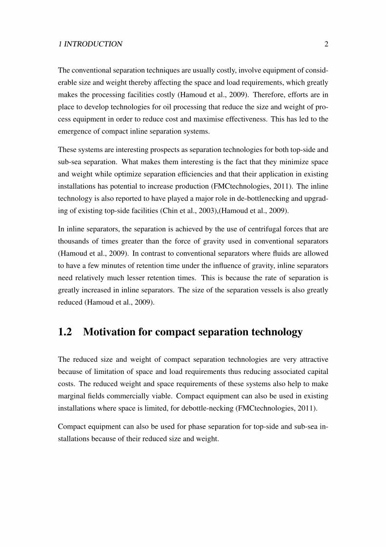
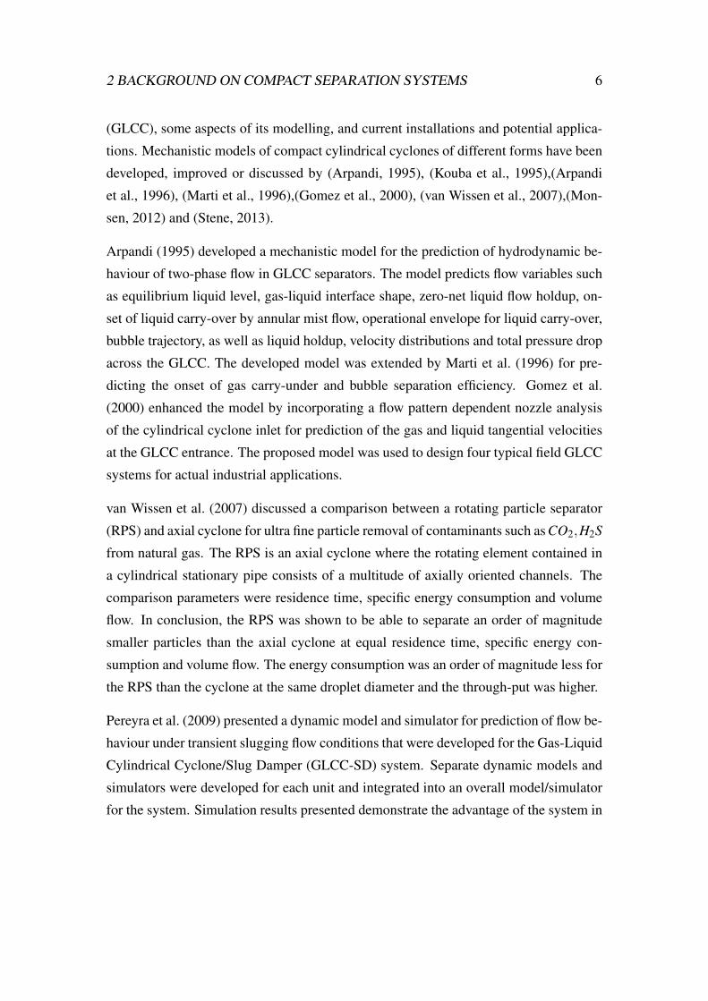
2.2 Compact separation system by Ellingsen
The compact separation system used for this work is that according to Ellingsen (2007)
as shown in figure 2.1 below.
As seen from figure 2.1, there are three separation units. Some of the units discussed
here are based on a new-inline technology where a centrifugal force is used to separate
the phases because of their difference in densities. This separation system is compact
because the units minimise space and weight and are designed to have almost the same
dimensions as the transport pipe thus inline-technology (Ellingsen, 2007).
The gravity separator does the bulk separation of the gas and liquid phases that enter the
unit. However, the separation obtained is not satisfactory as regards the demands of the
compressor and pump. Therefore, the degasser and deliquidizer do further separation
of the phases. The degasser separates gas from a liquid dominated stream while the
deliquidizer separates liquid from a gas dominated stream (FMCtechnologies, 2011).
2 BACKGROUND ON COMPACT SEPARATION SYSTEMS 9
Figure 2.1: Compact separation system by Ellingsen
Adapted from (Ellingsen, 2007)
2 BACKGROUND ON COMPACT SEPARATION SYSTEMS 10
It is important to note about the compact separation system in figure 2.1 that the oper-
ational objective is to adjust the available valves in such a way that the gas content in
the liquid stream to the pump is minimised. Therefore the quality of the liquid from
the degasser is more important than the gas quality and therefore the gas phase from the
degasser undergoes further separation in the deliquidizer.
Note that the return streams of liquid and gas after the pump and compressor are not
meant for use under normal operation. They are meant to ensure that there is enough
feed to the pump and compressor and that the flow rates through the deliquidizer and
degasser are above certain limits (Ellingsen, 2007).
2.3 Gravity separators
These are pressure vessels that separate a mixed stream of liquid and gas phases into
respective separate phases (Mokhatab and Poe, 2012). They employ the use of the
gravity forces to separate the mixed phases based on their differences in density. The
heavier phase settles at the bottom of the separator while the lightest rises to the top
but this requires some settling time. The larger the difference in density, the higher the
difference in velocity resulting in a lower settling time.
However, for large settling times, the separators need to be larger to effect the separation.
Due to the fact that large separator vessel sizes are required to achieve settling, gravity
separators are rarely designed to remove droplets smaller than 250 µm (Mokhatab and
Poe, 2012).
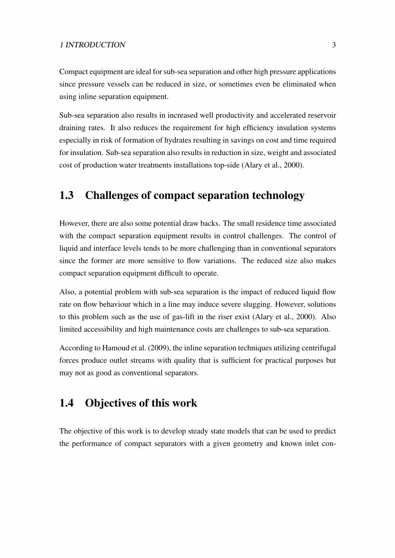
Gravity separators are often classified to be vertical or horizontal based on their geo-
metrical configuration or by their function. For example,they are “two-phase” if they
separate gas from a liquid stream (Mokhatab and Poe, 2012).
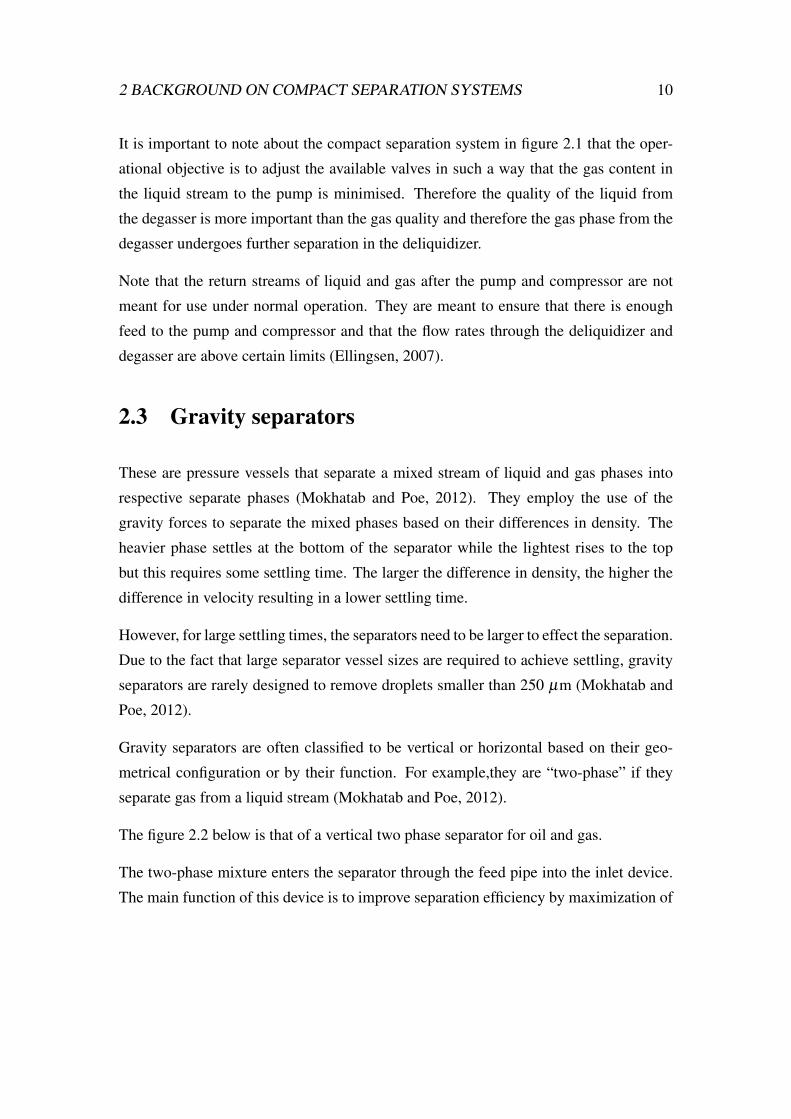
The figure 2.2 below is that of a vertical two phase separator for oil and gas.
The two-phase mixture enters the separator through the feed pipe into the inlet device.
The main function of this device is to improve separation efficiency by maximization of
2 BACKGROUND ON COMPACT SEPARATION SYSTEMS 11
Figure 2.2: Vertical gas liquid separator
gas/liquid separation efficiency, minimization of droplet shearing and provision of good
downstream velocity distributions of separated phases (Bothamley et al., 2013a).
In the gas gravity separation section, the entrained liquid load is reduced by separation
of liquid droplets from the gas phase. The mist extractor in addition is used to remove
liquid droplets remaining at the outlet of the gas gravity separation section.
On the other hand, free gas is separated out of the liquid in the liquid gravity separation
section (Bothamley et al., 2013b).
The separated gas and liquid phases exit at the top and bottom respectively.
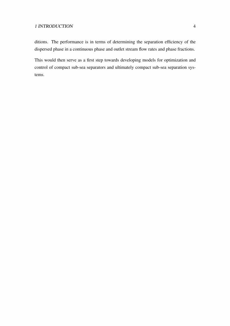
2.4 Deliquidizer
The deliqudizer is one of the units in the separation system discussed that is compact
and based on the inline technology. The role of the deliquidizer is to separate liquid
2 BACKGROUND ON COMPACT SEPARATION SYSTEMS 12
from the gas dominated stream from the gravity separator where bulk separation takes
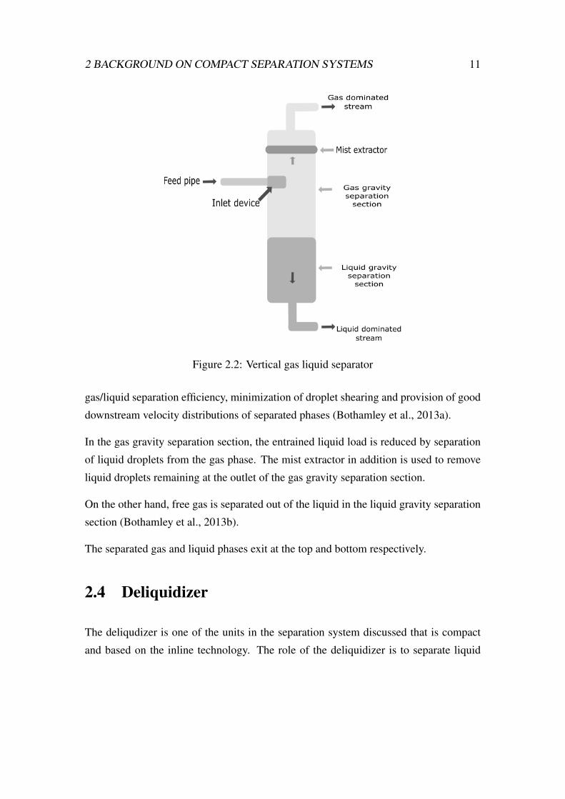
place. The components of a typical deliquidizer are shown in the figure 2.3 below.
Figure 2.3: Typical inline deliquidizer
Adapted from (FMCtechnologies)
The multiphase flow stream enters the unit through a flow conditioning element(1)
which equally distributes the liquid droplets throughout the pipe cross sectional area.
The stationary swirl element(2) then brings the two phase mixture into rotation which
causes the two phases to separate because of their difference in densities. The liquid
creates a thin film on the pipe’s outer wall and the gas exits through a small pipe in
the center of the main pipe(3) (Hamoud et al., 2009). The liquid enters the annular
space between the two pipes, hits the back wall of the deliquidizer and enters the boot
scetion(5). This liquid carries some gas and the latter is removed and recycled back
through the recycle line(6). The liquid is discharged at the bottom of the boot section.
The gas outlet pipe(4) has an anti-swirl element which stops the rotation, resulting in a
low-total pressure drop across the deliquidizer. The control of the deliquidizer will only
require level control for the liquid from the boot section (Hamoud et al., 2009).
2 BACKGROUND ON COMPACT SEPARATION SYSTEMS 13
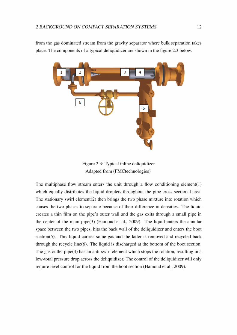
A successful deliquidizer installation as seen in figure 2.4 was implemented on the BP-
ETAP platform in the North sea in May 2003 (Schook et al., 2005). The ETAP deliq-
uidizer, a 20′′ unit was installed to reduce the amount of condensate that is eventually
carried by the HP gas cooler discharge drum to the downstream Glycol contactor, so as
to achieve the required water dew point of the export gas. The condensate caused prob-
lems for the Glycol contactor and Glycol regeneration unit resulting in financial losses
as a result of glycol losses and filter replacements.
Figure 2.4: BP ETAP deliquidizer installed on a platform in the North sea
Adapted from (Schook et al., 2005)
2.5 Degasser
The role of the degasser in the compact separation system here discussed is to separate
gas from the liquid stream from the gravity separator after bulk separation. This is also
a compact unit based on the inline technology.
2 BACKGROUND ON COMPACT SEPARATION SYSTEMS 14
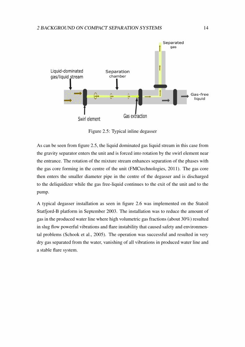
Figure 2.5: Typical inline degasser
As can be seen from figure 2.5, the liquid dominated gas liquid stream in this case from
the gravity separator enters the unit and is forced into rotation by the swirl element near
the entrance. The rotation of the mixture stream enhances separation of the phases with
the gas core forming in the centre of the unit (FMCtechnologies, 2011). The gas core
then enters the smaller diameter pipe in the centre of the degasser and is discharged
to the deliquidizer while the gas free-liquid continues to the exit of the unit and to the
pump.
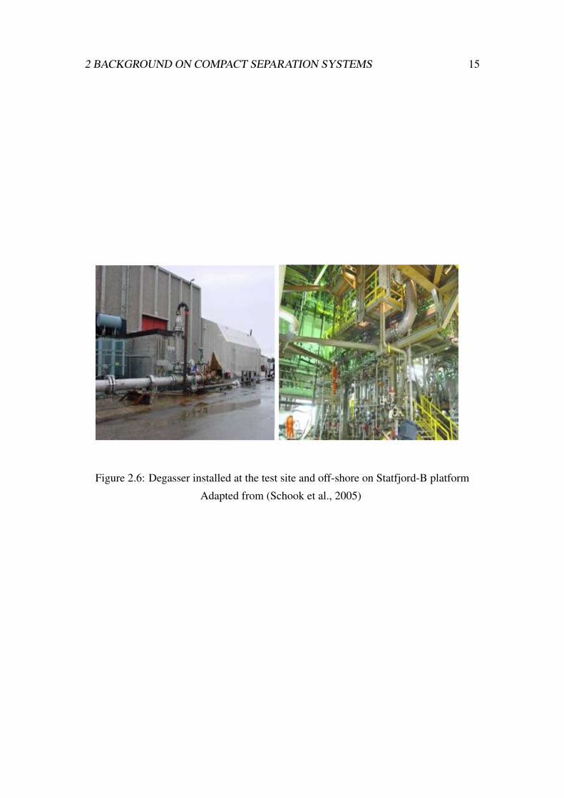
A typical degasser installation as seen in figure 2.6 was implemented on the Statoil
Statfjord-B platform in September 2003. The installation was to reduce the amount of
gas in the produced water line where high volumetric gas fractions (about 30%) resulted
in slug flow powerful vibrations and flare instability that caused safety and environmen-
tal problems (Schook et al., 2005). The operation was successful and resulted in very
dry gas separated from the water, vanishing of all vibrations in produced water line and
a stable flare system.
2 BACKGROUND ON COMPACT SEPARATION SYSTEMS 15
Figure 2.6: Degasser installed at the test site and off-shore on Statfjord-B platform
Adapted from (Schook et al., 2005)
3 MODELLING OF COMPACT SEPARATION SYSTEM UNITS 16
3 Modelling of Compact SeparationSystem Units
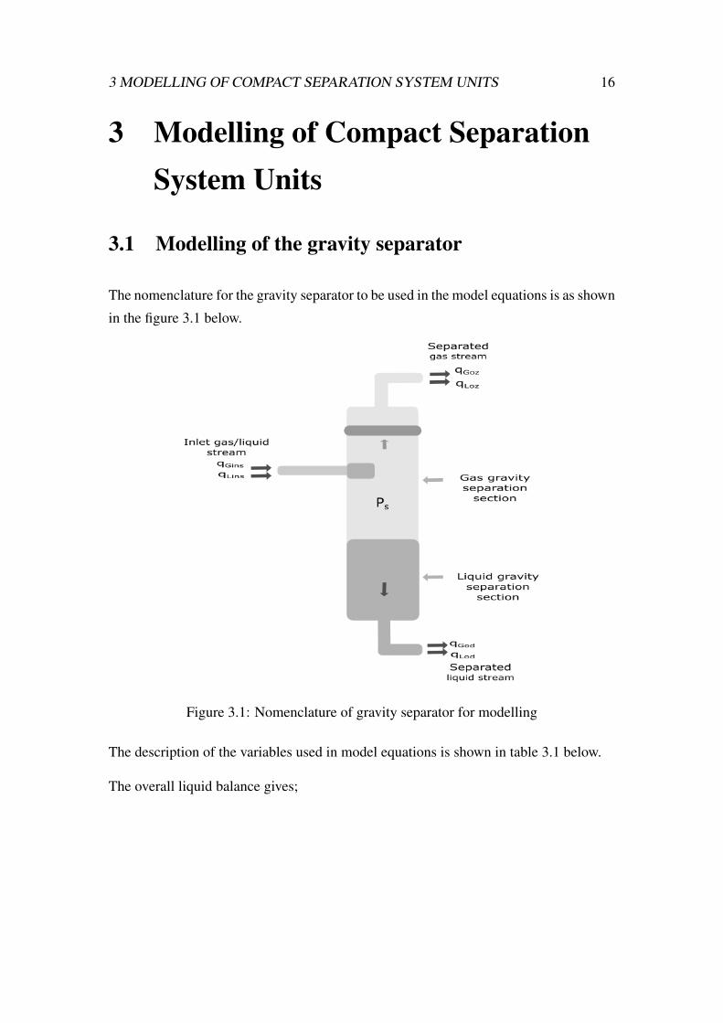
3.1 Modelling of the gravity separator
The nomenclature for the gravity separator to be used in the model equations is as shown
in the figure 3.1 below.
Figure 3.1: Nomenclature of gravity separator for modelling
The description of the variables used in model equations is shown in table 3.1 below.
The overall liquid balance gives;
3 MODELLING OF COMPACT SEPARATION SYSTEM UNITS 17
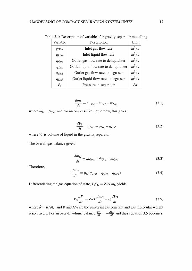
Table 3.1: Description of variables for gravity separator modellingVariable Description Unit
qGins Inlet gas flow rate m3/s
qLins Inlet liquid flow rate m3/s
qGoz Outlet gas flow rate to deliquidizer m3/s
qLoz Outlet liquid flow rate to deliquidizer m3/s
qGod Outlet gas flow rate to degasser m3/s
qLod Outlet liquid flow rate to degasser m3/s
Ps Pressure in separator Pa
dmL
dt= mLins− mLoz− mLod (3.1)
where mL = ρLqL and for incompressible liquid flow, this gives;
dVL
dt= qLins−qLoz−qLod (3.2)
where VL is volume of liquid in the gravity separator.
The overall gas balance gives;
dmG
dt= mGinz− mGoz− mGod (3.3)
Therefore,dmG
dt= ρG(qGins−qGoz−qGod) (3.4)
Differentiating the gas equation of state, PsVG = ZRT mG yields;
VGdPs
dt= ZRT
dmG
dt−Ps
dVG
dt(3.5)
where R = R/MG and R and MG are the universal gas constant and gas molecular weight
respectively. For an overall volume balance,dVLdt =−dVG
dt and thus equation 3.5 becomes;
3 MODELLING OF COMPACT SEPARATION SYSTEM UNITS 18
VGdPs
dt= ZRT
dmG
dt+Ps
dVL
dt(3.6)
For ρG = PsZRT , substituting equations 3.2, 3.4 into equation 3.6 gives;
VGdPs
dt= Ps(qGins−qGoz−qGod +(qLins−qLoz−qLod)) (3.7)
3.1.1 Entrainment in feed pipe
There are a variety of factors that are important in sizing and performance prediction
of most types of separation equipment such as the flow pattern at the separator inlet,
amount of dispersed phase present in entrained form and sizes of the droplets/bubbles.
However, there quantification is difficult and typically requires simplifying assumptions
(Bothamley et al., 2013a).
The flow pattern at the inlet is generally dependent on the relative amounts of gas and
liquid in the feed pipe and in-situ phase velocities (Bothamley et al., 2013a) but this
analysis is not considered further in this report. The focus is rather on the other factors.
We assume that the inlet flow pattern is in such a way that the phase velocities are
sufficiently large enough for dispersion of the phases to take place.
The amount of liquid entrainment as droplets in the gas significantly affects the sepa-
ration between the phases and increases with increasing gas velocities and decreasing
liquid surface tension (Bothamley et al., 2013a).
The liquid droplet entrainment has been predicted using a correlation developed for
annular flow by Pan and Hanratty (2002) but is also applicable to non-annular (lower
velocity) flows (Bothamley et al., 2013a). This correlation also includes a method of es-
timating the Sauter-mean diameter (d32) of the entrained liquid droplet size distribution
as shown in equation 3.8 below.
3 MODELLING OF COMPACT SEPARATION SYSTEM UNITS 19
(E/Em)
1− (E/Em)= 9e−08(
Du3g√
ρlρg
σ)(
ρ1−mg µm
g
d1+m32 gρl
)1
(2−m)
(ρgu2
gd32
σ)(
d32
D) = 0.0091,
(3.8)
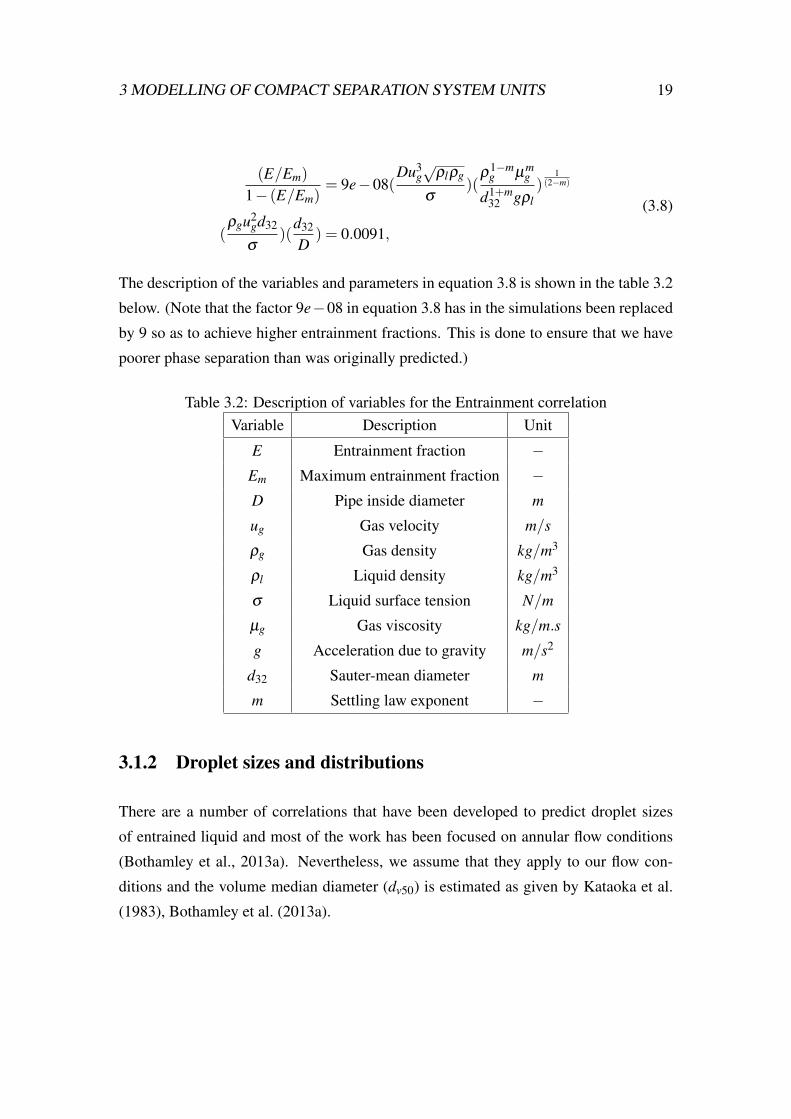
The description of the variables and parameters in equation 3.8 is shown in the table 3.2
below. (Note that the factor 9e−08 in equation 3.8 has in the simulations been replaced
by 9 so as to achieve higher entrainment fractions. This is done to ensure that we have
poorer phase separation than was originally predicted.)
Table 3.2: Description of variables for the Entrainment correlationVariable Description Unit
E Entrainment fraction −Em Maximum entrainment fraction −D Pipe inside diameter m
ug Gas velocity m/s
ρg Gas density kg/m3
ρl Liquid density kg/m3
σ Liquid surface tension N/m
µg Gas viscosity kg/m.s
g Acceleration due to gravity m/s2
d32 Sauter-mean diameter m
m Settling law exponent −
3.1.2 Droplet sizes and distributions
There are a number of correlations that have been developed to predict droplet sizes
of entrained liquid and most of the work has been focused on annular flow conditions
(Bothamley et al., 2013a). Nevertheless, we assume that they apply to our flow con-
ditions and the volume median diameter (dv50) is estimated as given by Kataoka et al.
(1983), Bothamley et al. (2013a).
3 MODELLING OF COMPACT SEPARATION SYSTEM UNITS 20
By definition, the volume median diameter (dv50) is the value where 50% of the total
volume of droplets is made up of droplets with diameters larger than the median value
and the rest smaller. The maximum droplet size is said to be in range 3-5 times dv50
(Bothamley et al., 2013a).
The volume median diameter is given by;
dv50 = 0.01(σ
ρgu2g)Re2/3
g (ρg
ρl)−1/3(
µg
µl)2/3
Reg =Dugρg
µg,
(3.9)
where µl is liquid viscosity and Reg is gas phase Reynolds number.
A look at equation 3.9 shows that the volume median diameter dv50 decreases with
increasing gas velocity, increasing gas density and decreasing surface tension.
Upper-Limit Log Normal distribution
The Upper-limit log normal distribution has been used by Simmons and Hanratty
(2001), Bothamley et al. (2013a) to represent droplets of entrained liquid in two-phase
flow.
The normalized volume frequency distribution is given as follows;
3 MODELLING OF COMPACT SEPARATION SYSTEM UNITS 21
fv(dp) =δdmax√
πdp(dmax−dp)exp(−δ
2z2)
where
z = ln(adp
dmax−dp)
a =dmax−dv50
dv50
δ =0.394
log(v90v50
)
vi =di
dmax−di
(3.10)
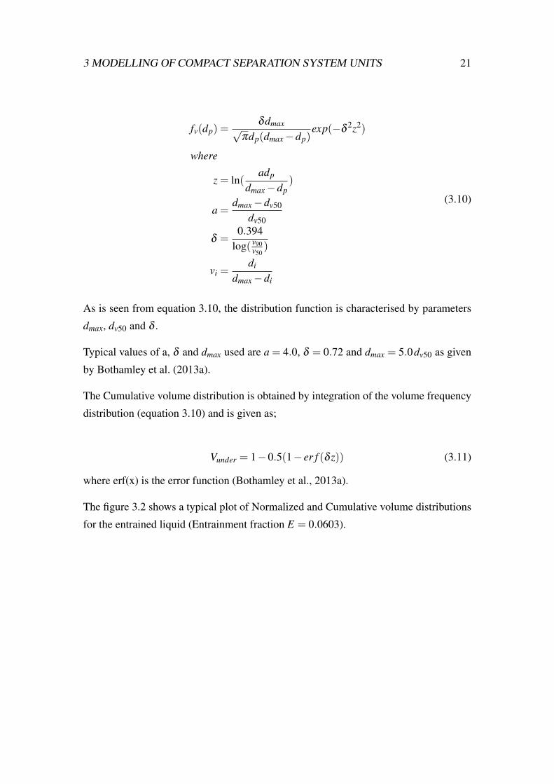
As is seen from equation 3.10, the distribution function is characterised by parameters
dmax, dv50 and δ .
Typical values of a, δ and dmax used are a = 4.0, δ = 0.72 and dmax = 5.0dv50 as given
by Bothamley et al. (2013a).
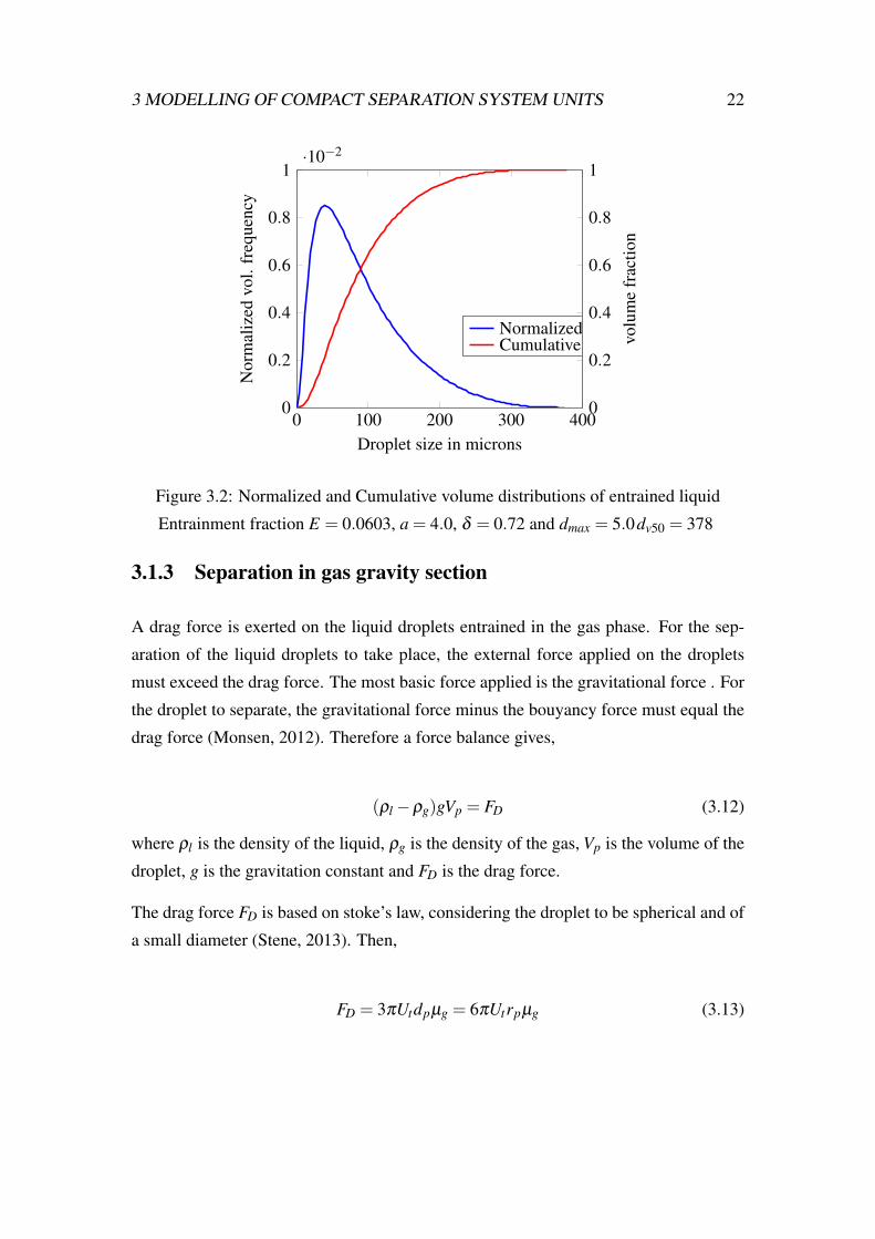
The Cumulative volume distribution is obtained by integration of the volume frequency
distribution (equation 3.10) and is given as;
Vunder = 1−0.5(1− er f (δ z)) (3.11)
where erf(x) is the error function (Bothamley et al., 2013a).
The figure 3.2 shows a typical plot of Normalized and Cumulative volume distributions
for the entrained liquid (Entrainment fraction E = 0.0603).
3 MODELLING OF COMPACT SEPARATION SYSTEM UNITS 22
0 100 200 300 4000
0.2
0.4
0.6
0.8
1·10−2
Droplet size in microns
Nor
mal
ized
vol.
freq
uenc
y
0
0.2
0.4
0.6
0.8
1
NormalizedCumulative vo
lum
efr
actio
n
Figure 3.2: Normalized and Cumulative volume distributions of entrained liquid
Entrainment fraction E = 0.0603, a = 4.0, δ = 0.72 and dmax = 5.0dv50 = 378
3.1.3 Separation in gas gravity section
A drag force is exerted on the liquid droplets entrained in the gas phase. For the sep-
aration of the liquid droplets to take place, the external force applied on the droplets
must exceed the drag force. The most basic force applied is the gravitational force . For
the droplet to separate, the gravitational force minus the bouyancy force must equal the
drag force (Monsen, 2012). Therefore a force balance gives,
(ρl−ρg)gVp = FD (3.12)
where ρl is the density of the liquid, ρg is the density of the gas, Vp is the volume of the
droplet, g is the gravitation constant and FD is the drag force.
The drag force FD is based on stoke’s law, considering the droplet to be spherical and of
a small diameter (Stene, 2013). Then,
FD = 3πUtdpµg = 6πUtrpµg (3.13)
3 MODELLING OF COMPACT SEPARATION SYSTEM UNITS 23
where Ut is the droplet terminal velocity, dp and rp are the droplet diameter and radius
respectively, µg is the gas viscosity. Therefore substituting for FD in equation 3.12 gives,
(ρl−ρg)gVp = 6πUtrpµg (3.14)
Substituting for Vp =43πr3
p in equation 3.14 and making Ut the subject gives,
Ut =2(ρl−ρg)gr2
p
9µg(3.15)
Therefore;
Ut =(ρl−ρg)gd2
p
18µg(3.16)
The above terminal velocity equation represents the stable velocity the droplet reaches
after an acceleration period in gas flow. The dependance of the terminal velocity on the
droplet diameter results in the fact that smaller droplets attain their terminal velocity
after a short time period than larger droplets (Stene, 2013).
The velocity profile of a continuous phase (gas, oil,or water) in a separator has histori-
cally been calculated from V = Q/A where Q is the in-situ volumetric flow rate of the
continuous phase and A is the cross-sectional area for flow (Bothamley et al., 2013a).
Therefore the gas velocity is given by;
ug =4Qg
πD2 (3.17)
where Qg is gas volumetric flow rate and D is the diameter of the gravity separator.
Therefore the terminal velocity of droplets Ut must be greater than or equal to the gas
velocity ug for the droplets to be separated from the gas phase.
For Ut = ug, it is possible to determine the “critical droplet size” d pcrit of the droplet
distribution above which all droplets are separated from the gas flow.
3 MODELLING OF COMPACT SEPARATION SYSTEM UNITS 24
d pcrit =
(72Qgµg
πD2(ρl−ρg)g
)1/2
(3.18)
From the cumulative volume distribution as given by equation 3.11, the volume fraction
of entrained liquid that remains in the gas flow is given by;
βcarry−over = 1−0.5(1− er f (δ zcrit)) (3.19)
where zcrit = ln(ad pcrit
dmax−d pcrit).
Therefore, the separation efficiency of the entrained liquid is given by;
ηe f f = 1−βcarry−over (3.20)
3.1.4 Gas and liquid volume fractions of exit streams
The gas volume fraction of the exiting gas stream at the top of the gravity separator is
given by;
αg =qGoz
qToz=
qGoz
qGoz +qLoz(3.21)
where qToz is the total outlet flow rate to deliquidizer.
Note; qLoz = qLinsEβcarry−over where E is the liquid entrainment fraction.
The liquid volume fraction of the exiting stream at the bottom of the gravity separator
is given by;
βl =qLod
qTod=
qLod
qLod +qGod(3.22)
where qLod = qLins−qLoz.
We note that the terms qGoz and qGod are unknown.
3 MODELLING OF COMPACT SEPARATION SYSTEM UNITS 25
Analogous to the analysis for the liquid dispersed in gas as has been discussed above,
we assume that gas is also dispersed into the liquid and behaves in a similar manner and
thus summarise the behaviour as follows;
The gas entrainment is predicted by;
(Eg/Em)
1− (Eg/Em)= 9(
Du3l√
ρlρg
σ)(
ρ1−ml µm
l
d1+m32g gρl
)1
(2−m)
(ρlu2
l d32g
σ)(
d32g
D) = 0.0091,
(3.23)
The volume median diameter of the bubble size distribution (dv50g)is given by;
dv50g = 0.01(σ
ρlu2l)Re2/3
l (ρl
ρg)−1/3(
µl
µg)2/3
Rel =Dulρl
µl,
(3.24)
The bubble rise velocity is given by an equation similar to that of the droplet terminal
velocity (equation 3.16) as given below;
Therefore;
Ur =(ρl−ρg)gd2
p
18µl(3.25)
The liquid velocity is also given by;
ul =4Ql
πD2 (3.26)
where Ql is liquid volumetric flow rate and D is the diameter of the gravity separator.
Therefore the bubble rise velocity Ur must be greater than or equal to the liquid velocity
ul for the bubbles to be separated from the liquid phase.
3 MODELLING OF COMPACT SEPARATION SYSTEM UNITS 26
For Ur = ul , the “critical bubble size” d pcritg of the bubble size distribution above which
all bubbles are large enough to be separated from the liquid is given by;
d pcritg =
(72Qlµl
πD2(ρl−ρg)g
)1/2
(3.27)
From the cumulative volume distribution as given by equation 3.11, the volume fraction
of entrained gas that remains in the liquid flow is given by;
βcarry−under = 1−0.5(1− er f (δ zcritg)) (3.28)
where zcritg = ln(ad pcritg
dmaxg−d pcritg) and dmaxg = 5dv50g.
Therefore, the separation efficiency of the entrained gas is given by;
ηe f f g = 1−βcarry−under (3.29)
Therefore, the amount of gas carried with the liquid stream exiting at the bottom of the
gravity separator is given by;
qGod = qGinsEgβcarry−under (3.30)
where Eg is the gas entrainment fraction.
Thus; qGoz = qGins−qGod . Therefore, the phase fractions as defined by equations 3.21
and 3.22 can be determined.
3 MODELLING OF COMPACT SEPARATION SYSTEM UNITS 27
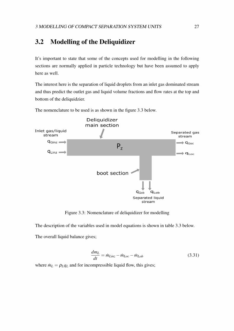
3.2 Modelling of the Deliquidizer
It’s important to state that some of the concepts used for modelling in the following
sections are normally applied in particle technology but have been assumed to apply
here as well.
The interest here is the separation of liquid droplets from an inlet gas dominated stream
and thus predict the outlet gas and liquid volume fractions and flow rates at the top and
bottom of the deliquidzier.
The nomenclature to be used is as shown in the figure 3.3 below.
Figure 3.3: Nomenclature of deliquidizer for modelling
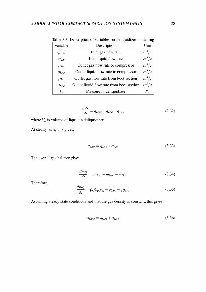
The description of the variables used in model equations is shown in table 3.3 below.
The overall liquid balance gives;
dmL
dt= mLinz− mLoc− mLob (3.31)
where mL = ρLqL and for incompressible liquid flow, this gives;
3 MODELLING OF COMPACT SEPARATION SYSTEM UNITS 28
Table 3.3: Description of variables for deliquidizer modellingVariable Description Unit
qGinz Inlet gas flow rate m3/s
qLinz Inlet liquid flow rate m3/s
qGoc Outlet gas flow rate to compressor m3/s
qLoc Outlet liquid flow rate to compressor m3/s
qGob Outlet gas flow rate from boot section m3/s
qLob Outlet liquid flow rate from boot section m3/s
Pz Pressure in deliquidizer Pa
dVL
dt= qLinz−qLoc−qLob (3.32)
where VL is volume of liquid in deliquidizer.
At steady state, this gives;
qLinz = qLoc +qLob (3.33)
The overall gas balance gives;
dmG
dt= mGinz− mGoc− mGob (3.34)
Therefore,dmG
dt= ρG(qGinz−qGoc−qGob) (3.35)
Assuming steady state conditions and that the gas density is constant, this gives;
qGinz = qGoc +qGob (3.36)
3 MODELLING OF COMPACT SEPARATION SYSTEM UNITS 29
3.2.1 Cyclonic separation in the deliquidizer
In this subsection, modelling of cyclonic separation is considered where the forces
present push the heavier liquid phase outwards to the wall while the lighter gas phase
remains in the middle section. The external forces (centrifugal forces) generated in
this case are greater than the gravitational forces used in conventional separators and
therefore retention times for phase separation are greatly reduced.
Radial velocity
A look at equation 3.15 shows that the external force involved is the gravitational force.
However, for cyclonic separation, there are centrifugal forces, thus the centripetal ac-
celeration ac which is assumed to have a greater influence on the droplet than gravity
replaces the gravitational acceleration g in the above equation (Stene, 2013). The cen-
tripetal acceleration ac is given by ac =u2
tr where ut is the tangential velocity and r the
radial position.
In a cylindrical geometry, equation 3.15 can now be written as;
ur =drdt
=(ρl−ρg)d2
pu2t
18µgr(3.37)
The swirl flow in the deliquidizer is assumed to be a forced vortex flow, which is swirling
flow with the same tangential velocity distribution as a rotating solid body as opposed to
free vortex flow, the way a frictionless fluid would swirl. This is done for simplicity as
the tangential velocity distribution for real swirling flows is intermediate between these
two extreme cases (Hoffmann and Stein, 2002). In addition, Swanborn (1988) shows
that the tangential velocity distribution at the inlet is close to a forced vortex and perhaps
our assumption is not as bad since we consider conditions at the inlet but the validity of
this assumption has not been justified.
For a forced vortex flow, the tangential velocity ut is given by ut = ωr where ω is the
angular velocity measured in radians per unit of time and is a constant for a forced
3 MODELLING OF COMPACT SEPARATION SYSTEM UNITS 30
vortex flow (Hoffmann and Stein, 2002). Substituting for ut in equation 3.37 gives
ur =drdt
=(ρl−ρg)d2
pω2r18µg
(3.38)
Time of flight model
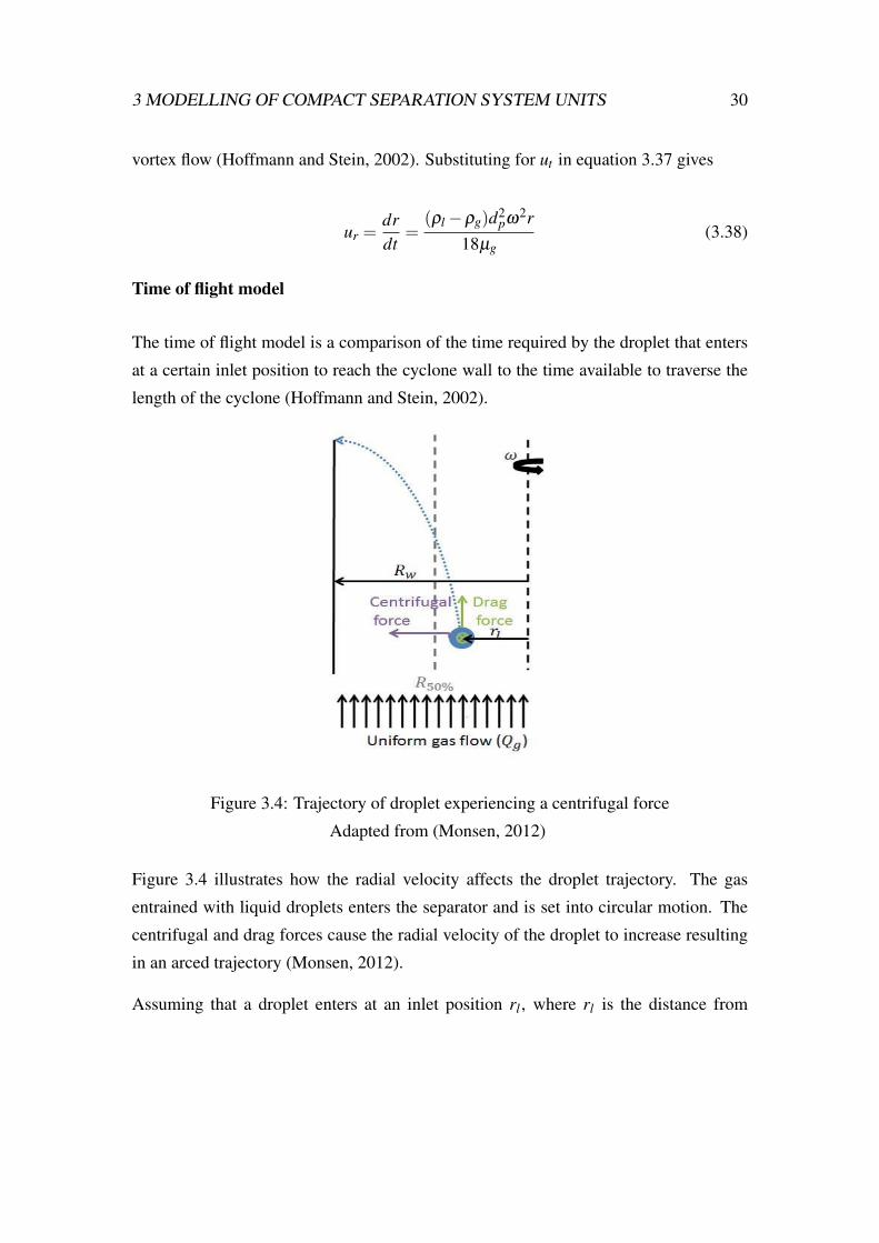
The time of flight model is a comparison of the time required by the droplet that enters
at a certain inlet position to reach the cyclone wall to the time available to traverse the
length of the cyclone (Hoffmann and Stein, 2002).
Figure 3.4: Trajectory of droplet experiencing a centrifugal force
Adapted from (Monsen, 2012)
Figure 3.4 illustrates how the radial velocity affects the droplet trajectory. The gas
entrained with liquid droplets enters the separator and is set into circular motion. The
centrifugal and drag forces cause the radial velocity of the droplet to increase resulting
in an arced trajectory (Monsen, 2012).
Assuming that a droplet enters at an inlet position rl , where rl is the distance from
3 MODELLING OF COMPACT SEPARATION SYSTEM UNITS 31
the its inlet position to the separator centre, the time tradial for the droplet to reach the
separator wall R can be obtained by integration of equation 3.38 from rl to R (Monsen,
2012). This gives;
tradial =18µg
(ρl−ρg)d2pω2 ln
Rrl
(3.39)
On the other hand, the time taxial available for the droplet from the inlet to exit of the
separator is given by;
taxial =Lvz
=πR2LqTinz
(3.40)
where L is the length of the separator, vz is the axial velocity and qTinz is the total inlet
volumetric flow rate.
A comparison of tradial and taxial leads to possible cases. Either tradial is less than taxial ,
implying that the liquid droplet will reach the wall before exiting the separator thus
separating from gas flow. Or tradial is greater than taxial , implying that the liquid droplet
will not reach the wall of the separator and remains entrained in the gas flow (Monsen,
2012).
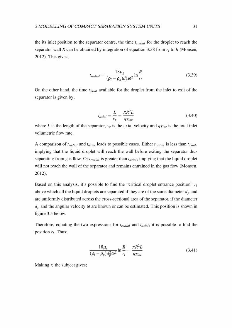
Based on this analysis, it’s possible to find the “critical droplet entrance position” rl
above which all the liquid droplets are separated if they are of the same diameter dp and
are uniformly distributed across the cross-sectional area of the separator, if the diameter
dp and the angular velocity ω are known or can be estimated. This position is shown in
figure 3.5 below.
Therefore, equating the two expressions for tradial and taxial , it is possible to find the
position rl . Thus;
18µg
(ρl−ρg)d2pω2 ln
Rrl=
πR2LqTinz
(3.41)
Making rl the subject gives;
3 MODELLING OF COMPACT SEPARATION SYSTEM UNITS 32
Figure 3.5: Theoretical cross sectional view of the critical droplet entrance position rl
for separation
rl = exp(lnR−(ρl−ρg)d2
pω2πR2L18µgqTinz
) (3.42)
rl = exp(lnR−(ρl−ρg)d2
pω2taxial
18µg) (3.43)
It’s quite obvious from equation 3.42 that rl is dependent on the inlet volumetric flow
rate qTinz, angular velocity ω , droplet diameter dp, density difference between the
phases to be separated ρl − ρg, viscosity of the continuous phase µg and the length
L and radius R of the separator.
Uniform droplet distribution
It’s assumed in this model that all the liquid is dispersed into droplets of a certain size,
diameter dp that are distributed uniformly into the gas phase. This assumption is sup-
ported by the fact that there is a mixing element at the start of the deliquidizer whose
role is to equally distribute the liquid droplets throughout the pipe cross sectional area.
Let n be the total number of droplets entering the unit. The number of droplets per
unit cross sectional area na =n
πR2 . The number of droplets separated nsep (with tradial
3 MODELLING OF COMPACT SEPARATION SYSTEM UNITS 33
less than taxial) are in the cross sectional area π(R2− r2l ). Thus nsep = naπ(R2− r2
l ) =
n(1− ( rlR )
2).
Therefore, volume separated Vsep = n(1− ( rlR )
2)Vp where Vp =43πr3
p is the volume of
each droplet. But nVp is the total volume of liquid into the separator. Therefore the vol-
umetric flow rate of liquid separated Vsep = qLinz(1−( rlR )
2) where qLinz is the volumetric
flow rate of liquid into the separator. If qTinz is the total inlet volumetric flow rate and f
is the gas volume fraction, then qLinz = (1− f )qTinz. Therefore, Vsep is given by;
Vsep = (1− f )qTinz(1− (rl
R)2) (3.44)
The equation 3.44 predicts the volumetric flow rate of liquid separated from the gas
phase in the deliquidizer. Note that rl is dependent on other parameters as previously
discussed in this subsection. Therefore, the volumetric flow rate of liquid separated Vsep
is similarly dependent on the same parameters.
On the other hand, a closer look at figure 3.5 shows that the liquid separation efficiency
can be determined, thus;
ηe f f =Areaaboverl
Crosssectional area=
R2− r2l
R2 (3.45)
Phase fractions of exit streams
Finally, the gas volume fraction αg of the exiting stream after separation of the liquid is
given by;
αg =qToc−qLoc
qToc(3.46)
where qToc = qGoc +qLoc
The top flow rate qToc = F ∗qTinz where F is the split fraction and qTinz is the total inlet
flow rate and both F and qTinz are assumed to be known.
3 MODELLING OF COMPACT SEPARATION SYSTEM UNITS 34
Assuming that all the separated liquid exits the deliquidizer through the bottom, then
qLob = Vsep and qLoc = qLinz−qLob. Thus αg can be determined.
We have not considered separation in the boot section of the deliquidizer and thus as-
sume that all the gas and liquid that does not leave through the top outlet stream ex-
its through the bottom stream. Therefore, the liquid volume fraction βl of the bottom
stream is given by;
βl =qLob
qLob +qGob(3.47)
Effective swirl
The concept of “Effective swirl" in this case has been used to represent a variation of
angular velocity ω with inlet volumetric flow rate and its definition does not stand for
the term “swirl" as applied in fluid dynamics.
The representation of this concept for the purposes of this report is a Gompertz function
of the form (ref Wikipedia);
y(t) = a∗ exp(−b∗ exp(−c∗ t)) (3.48)
where a is an asymptote, b sets the displacement along the x-axis and c sets the growth
rate(y scaling). b and c are positive numbers. This is a sigmoid function where growth is
slowest at the start and end of the independent variable. Therefore, the angular velocity
as a function of the inlet volumetric flow rate is represented as given by equation 3.49
below.
ω = a∗ exp(−b∗ exp(−c∗qTinz)) (3.49)
This representation of the angular velocity as a Gompertz function was used in the
model and predictions obtained were compared to data.
3 MODELLING OF COMPACT SEPARATION SYSTEM UNITS 35
The representation of angular velocity as a simple power function of the volumetric
flow rate was also tried for comparison purposes to determine which of the functions
best represented the angular velocity. The Gompertz function representation produced
better predictions and is further used in this report.
The lsqcurvefit in Matlab was used to find parameters a,b,c for the gompertz function
that best fit the model outlet gas volume fraction predictions to experimental data (This
experimental data is found in mod_deliq in Appendix A.1 ).
Model improvement to cater for phase mix-up after separation
The concept of droplet breakup at high Reynold’s numbers was used to improve the
model. According to Van Campen (2014), the acceleration of a dispersed liquid-liquid
system can lead to droplet breakup. Droplets exist due to interfacial tension force and
forces acting on the interface, such as shear and viscous forces cause droplet deforma-
tion. If these forces exceed the interfacial tension force by a critical extent, the droplet
breaks into two or more smaller droplets.
Even though Van Campen (2014) discusses liquid-liquid systems, we have used the idea
of droplet breakup for a gas-liquid system. He further states that Hinze (1955) proposed
a model for the maximum droplet size in turbulent flow as follows;
Dmax(ρc
σ)3/5
ε2/5 = 0.725 (3.50)
where ρc is the density of the continuous phase, σ is the interfacial tension and ε the
turbulent dissipation rate. The turbulent length scale can be estimated by;
l = (v3
ε)1/4 = loRe−3/4 (3.51)
where v is the kinematic viscosity and lo the scale of the largest eddy (the tube diameter).
The turbulent kinetic energy can then be expressed as;
3 MODELLING OF COMPACT SEPARATION SYSTEM UNITS 36
ε =v3Re3
l4o
=u3
D(3.52)
where u is average velocity and D is tube diameter.
Also, u = 4qTinzπD2 where qTinz is the volumetric flow rate. Substituting for ε in equation
3.50 gives;
Dmax = 0.725(σ
ρc)3/5(
π3D7
64q3Tinz
)2/5 (3.53)
The equation 3.53 show a relationship between the droplet size Dmax and volumetric
flow rate qTinz. For the case of simplicity, an inverse linear relationship of the form
Dmax = mqTinz + c with m and c being the slope and intercept respectively was used
for improvement of model predictions. The parameters m and c were determined by
validation of the model predictions against experimental data.
3 MODELLING OF COMPACT SEPARATION SYSTEM UNITS 37
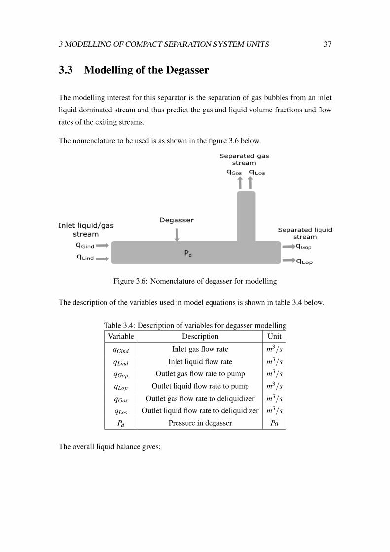
3.3 Modelling of the Degasser
The modelling interest for this separator is the separation of gas bubbles from an inlet
liquid dominated stream and thus predict the gas and liquid volume fractions and flow
rates of the exiting streams.
The nomenclature to be used is as shown in the figure 3.6 below.
Figure 3.6: Nomenclature of degasser for modelling
The description of the variables used in model equations is shown in table 3.4 below.
Table 3.4: Description of variables for degasser modellingVariable Description Unit
qGind Inlet gas flow rate m3/s
qLind Inlet liquid flow rate m3/s
qGop Outlet gas flow rate to pump m3/s
qLop Outlet liquid flow rate to pump m3/s
qGos Outlet gas flow rate to deliquidizer m3/s
qLos Outlet liquid flow rate to deliquidizer m3/s
Pd Pressure in degasser Pa
The overall liquid balance gives;
3 MODELLING OF COMPACT SEPARATION SYSTEM UNITS 38
dmLd
dt= mLind− mLos− mLop (3.54)
where mLd = ρLqL and for incompressible liquid flow, this gives;
dVLd
dt= qLind−qLos−qLop (3.55)
where VLd is volume of liquid in degasser.
At steady state, we obtain;
qLind = qLos +qLop (3.56)
The overall gas balance gives;
dmGd
dt= mGind− mGos− mGop (3.57)
Therefore,dmGd
dt= ρG(qGind−qGos−qGop) (3.58)
Assuming steady state conditions and that the gas density is constant, we obtain;
qGind = qGos +qGop (3.59)
3.3.1 Cyclonic separation in the degasser
The approach used in this case is similar to that as was used for the deliquidizer. How-
ever, we now have gas bubbles dispersed in a liquid stream which are separated to form a
gas core in the centre of the degasser. The forces that apply are similar as was discussed
in subsection 3.2.1.
We therefore consider the radial velocity of the gas bubbles experiencing centripetal
acceleration as given by;
3 MODELLING OF COMPACT SEPARATION SYSTEM UNITS 39
ur =drdt
=(ρg−ρl)d2
pu2t
18µlr(3.60)
where ut is the tangential velocity.
The vortex associated with cyclonic separation is a combined vortex with a forced vortex
in the central region and a free vortex on the outside of the region (Monsen, 2012).
However, we once again consider the vortex to be a forced vortex and therefore the
tangential velocity is given as follows.
ut = 2πrω (3.61)
where ω is the angular frequency.
Let us consider a gas bubble entering the separator at radial position r = rin, the radial
time it takes to reach the gas pipe radius r = rpp is given by substitution of 3.61 into
3.60 and integration yields;
tradial =18µl
4π2(ρg−ρl)d2pω2 ln
rpp
rin(3.62)
On the other hand, the time taxial available for the bubble from the inlet to exit of the
separator is given by;
taxial =Luz
=πR2LqTind
(3.63)
where L is the length of the separator, uz is the axial velocity and qTind is the total inlet
volumetric flow rate.
A comparison of tradial and taxial leads to possible cases. Either tradial is less than taxial ,
implying that the gas bubble will be separated. Or tradial is greater than taxial , imply-
ing that the gas bubble will not reach the gas core in the separator centre and remains
entrained in the liquid.
3 MODELLING OF COMPACT SEPARATION SYSTEM UNITS 40
Therefore it’s possible to find the “critical bubble entrance position” rl below which all
the gas bubbles are separated if they are of the same diameter dp and are uniformly
distributed across the cross-sectional area of the separator. This gives;
18µl
4π2(ρg−ρl)d2pω2 ln
rpp
rl=
πR2LqTind
(3.64)
Making rl the subject gives;
rl = exp(lnrpp−4π2(ρg−ρl)d2
pω2πR2L18µlqTind
) (3.65)
Therefore;
rl = rpp exp(−4π2(ρg−ρl)d2
pω2taxial
18µl) (3.66)
Uniform droplet distribution and separation efficiency
Assuming that the gas phase is uniformly dispersed into bubbles of a certain size, di-
ameter dp that are distributed uniformly over the entire cross sectional area. Figure 3.7
below shows a cross-sectional view of the “critical bubble entrance position rl”.
We assume that all the gas bubbles below the “critical bubble entrance position rl” are
separated. Thus the separation efficiency η of the degasser is predicted as follows;
η =π(r2
l − r2pp)
π(R2− r2pp)
(3.67)
The flow rate of separated gas qgsep is obtained as a product of gas flow rate into the
degasser and separation efficiency, thus;
qgsep = qGind(r2
l − r2pp)
(R2− r2pp)
(3.68)
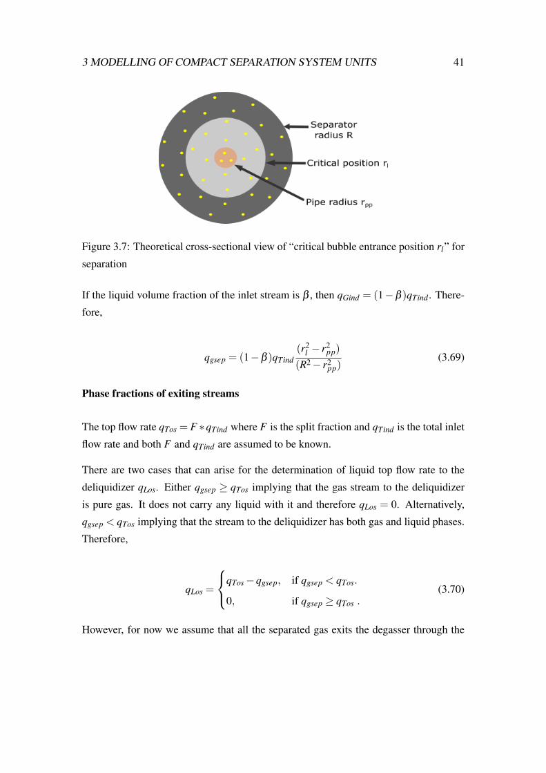
3 MODELLING OF COMPACT SEPARATION SYSTEM UNITS 41
Figure 3.7: Theoretical cross-sectional view of “critical bubble entrance position rl” for
separation
If the liquid volume fraction of the inlet stream is β , then qGind = (1−β )qTind . There-
fore,
qgsep = (1−β )qTind(r2
l − r2pp)
(R2− r2pp)
(3.69)
Phase fractions of exiting streams
The top flow rate qTos = F ∗qTind where F is the split fraction and qTind is the total inlet
flow rate and both F and qTind are assumed to be known.
There are two cases that can arise for the determination of liquid top flow rate to the
deliquidizer qLos. Either qgsep ≥ qTos implying that the gas stream to the deliquidizer
is pure gas. It does not carry any liquid with it and therefore qLos = 0. Alternatively,
qgsep < qTos implying that the stream to the deliquidizer has both gas and liquid phases.
Therefore,
qLos =
qTos−qgsep, if qgsep < qTos.
0, if qgsep ≥ qTos .(3.70)
However, for now we assume that all the separated gas exits the degasser through the
3 MODELLING OF COMPACT SEPARATION SYSTEM UNITS 42
top stream, then qGos = qgsep and qLos = qTos−qGos.
The gas volume fraction αg of the top exiting stream can be determined as follows;
αg =qGos
qTos(3.71)
Finally, the liquid volume fraction βl of the exiting bottom stream to the pump, after
separation of the gas is given by;
βl =qLop
qTind−qTos(3.72)
where qLop = qLind−qLos
4 OPTIMIZATION 43
4 Optimization
The main reason for focusing on optimization is the consideration of the performance
of a process. The goal of an optimization problem is to minimize an objective function
J subject to given equality and inequality constraints g and h respectively. Therefore, a
steady state optimization problem can be formulated as follows (Rangaiah and Kariwala,
2012);
minu J(u,x,d)
subject to constraints:
g(u,x,d) = 0
h(u,x,d)≤ 0
(4.1)
where u, x and d are steady state degrees of freedom, states and disturbances respec-
tively. g represents equality constraints that include model equations which relate the
independent variables (u and d) to the states(x) and h represents inequality constraints
(such as non-negative flows, volume fractions less or equal to 1). Therefore the system
must satisfy the given inequality constraints. In most cases, some subset h′ of the in-
equality constraints h are active (h′= 0 at the optimal solution). These active constraints
are satisfied by adjusting a corresponding number of degrees of freedom (Skogestad,
2004).
4.1 Problem formulation
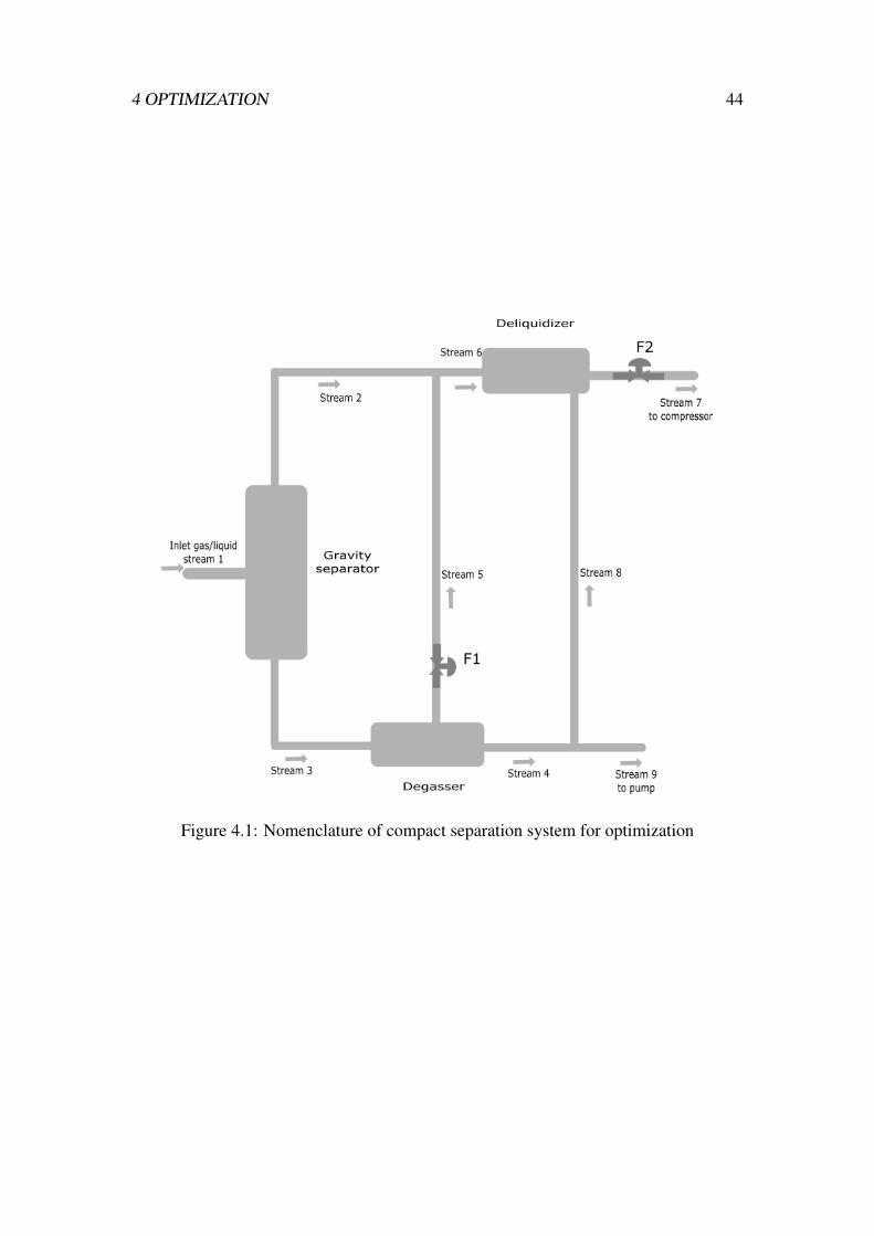
Th figure 4.1 below shows the compact separation system for optimization. All variables
corresponding to a given stream shall be denoted by the respective stream number for
example qg1, f1 denote the volumetric flow rate and gas volume fraction of stream 1.
The manipulated variables are assumed to be the split fractions (F1 and F2) on the
degasser and deliquidizer respectively. These are fractions of the total inlet flow rates
and set the total outlet flow rates of the top streams exiting the degasser and deliquidizer.
4 OPTIMIZATION 44
Figure 4.1: Nomenclature of compact separation system for optimization
4 OPTIMIZATION 45
We assume that there is no degree of freedom on the gravity separator since the model
as described in section 3.1 fixes the output flow rates and phase fractions for a fixed inlet
flow rate and gas volume fraction if other parameters are kept constant. The disturbance
variables are assumed to be the volumetric flow rate and phase fraction of the gas/liquid
stream to the gravity separator (stream 1). The output variables are the flow rates and
phase fractions ( f and β being gas and liquid volume fractions) of streams exiting the
separators.
The objective here is to have an acceptable (near-optimal) operation of the system with
the maximum achievable gas and liquid volume fractions of the streams exiting to the
compressor and pump respectively. This translates to the minimization of the amounts
of liquid in the gas stream to the compressor and gas in the liquid stream to the pump.
The presence of a condensate or water in a gas to the compressor results in a reduction
in compressor performance, compressor corrosion and increases the mechanical stress
on the impellers due to an increased mass flow rate (Brenne et al., 2008). Therefore,
it’s advantageous from an economical point of view to reduce this liquid amount to a
minimum. In addition, the presence of gas in liquid to the pump is also considered
detrimental to the performance and life of a pump and therefore this amount of gas
should also be minimized.
4.2 Objective function
We wish to maximize the average of gas and liquid volume fractions of streams 7 and
9 respectively. The optimization has been done in Matlab using f mincon as the solver
and since Matlab optimization solvers handle only minimization problems, the maxi-
mization problem is defined as negative function. Thus, the objective function J is as
follows;
J(F1,F2) =−0.5( f7 +β9) (4.2)
4 OPTIMIZATION 46
where f7 and β9 are gas and liquid fractions of streams 7 and 9 to the compressor and
pump respectively. They are also functions of F1 and F2. The 0.5 in equation 4.2 is to
take an average of phase fractions f7and β9 so that the objective function value also lies
between 0 and 1.
A combination of the models of the three separation units gives a complete model for
the compact separation system. The complete model outputs are phase fractions f7,β9
and flow rates q7, qg7, ql7, q9, qg9 and ql9.
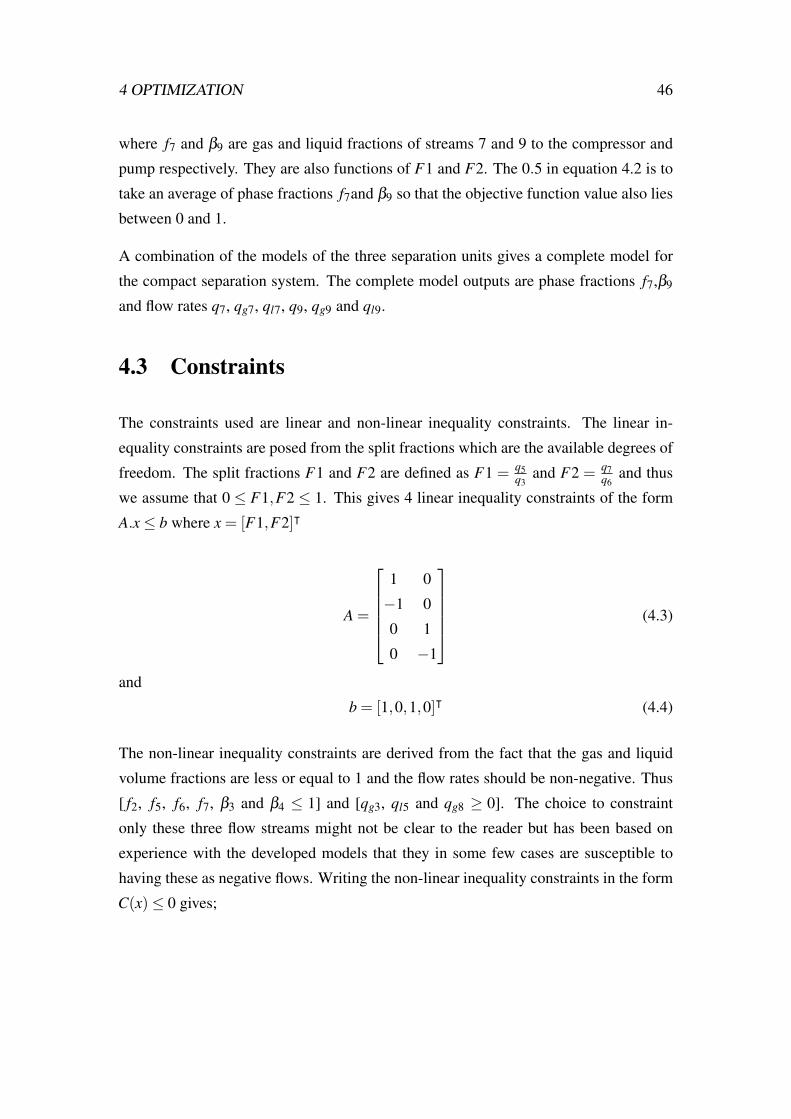
4.3 Constraints
The constraints used are linear and non-linear inequality constraints. The linear in-
equality constraints are posed from the split fractions which are the available degrees of
freedom. The split fractions F1 and F2 are defined as F1 = q5q3
and F2 = q7q6
and thus
we assume that 0 ≤ F1,F2 ≤ 1. This gives 4 linear inequality constraints of the form
A.x≤ b where x = [F1,F2]ᵀ
A =
1 0
−1 0
0 1
0 −1
(4.3)
and
b = [1,0,1,0]ᵀ (4.4)
The non-linear inequality constraints are derived from the fact that the gas and liquid
volume fractions are less or equal to 1 and the flow rates should be non-negative. Thus
[ f2, f5, f6, f7, β3 and β4 ≤ 1] and [qg3, ql5 and qg8 ≥ 0]. The choice to constraint
only these three flow streams might not be clear to the reader but has been based on
experience with the developed models that they in some few cases are susceptible to
having these as negative flows. Writing the non-linear inequality constraints in the form
C(x)≤ 0 gives;
4 OPTIMIZATION 47
C = [ f2−1, f5−1, f6−1, f7−1,β3−1,β4−1,−qg3,−ql5,−qg8]ᵀ (4.5)
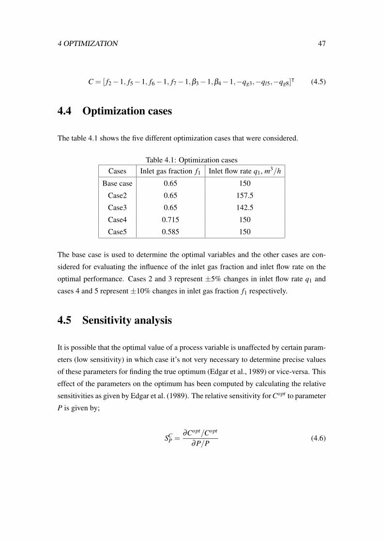
4.4 Optimization cases
The table 4.1 shows the five different optimization cases that were considered.
Table 4.1: Optimization casesCases Inlet gas fraction f1 Inlet flow rate q1, m3/h
Base case 0.65 150
Case2 0.65 157.5
Case3 0.65 142.5
Case4 0.715 150
Case5 0.585 150
The base case is used to determine the optimal variables and the other cases are con-
sidered for evaluating the influence of the inlet gas fraction and inlet flow rate on the
optimal performance. Cases 2 and 3 represent ±5% changes in inlet flow rate q1 and
cases 4 and 5 represent ±10% changes in inlet gas fraction f1 respectively.
4.5 Sensitivity analysis
It is possible that the optimal value of a process variable is unaffected by certain param-
eters (low sensitivity) in which case it’s not very necessary to determine precise values
of these parameters for finding the true optimum (Edgar et al., 1989) or vice-versa. This
effect of the parameters on the optimum has been computed by calculating the relative
sensitivities as given by Edgar et al. (1989). The relative sensitivity for Copt to parameter
P is given by;
SCP =
∂Copt/Copt
∂P/P(4.6)
4 OPTIMIZATION 48
where C is the objective function value and optimization variables F1 and F2 and P are
parameters q1 and f1.
The optimization results are shown and discussed in section 5.2.
5 RESULTS AND DISCUSSION 49
5 Results and discussion
All results presented in this chapter are generated in Matlab by implementation of the
models developed in the previous chapters. All the necessary Matlab codes are attached
in Appendix A.
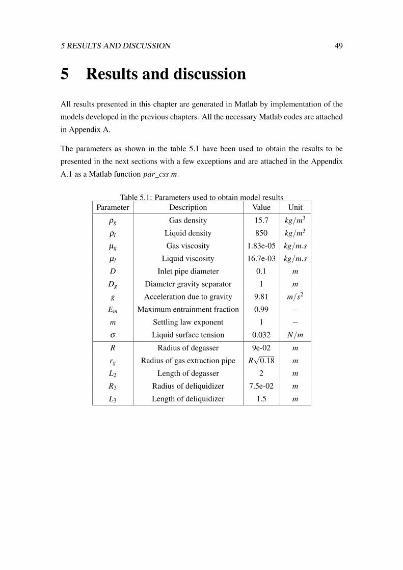
The parameters as shown in the table 5.1 have been used to obtain the results to be
presented in the next sections with a few exceptions and are attached in the Appendix
A.1 as a Matlab function par_css.m.
Table 5.1: Parameters used to obtain model resultsParameter Description Value Unit
ρg Gas density 15.7 kg/m3
ρl Liquid density 850 kg/m3
µg Gas viscosity 1.83e-05 kg/m.s
µl Liquid viscosity 16.7e-03 kg/m.s
D Inlet pipe diameter 0.1 m
Dg Diameter gravity separator 1 m
g Acceleration due to gravity 9.81 m/s2
Em Maximum entrainment fraction 0.99 −m Settling law exponent 1 −σ Liquid surface tension 0.032 N/m
R Radius of degasser 9e-02 m
rg Radius of gas extraction pipe R√
0.18 m
L2 Length of degasser 2 m
R3 Radius of deliquidizer 7.5e-02 m
L3 Length of deliquidizer 1.5 m
5 RESULTS AND DISCUSSION 50
5.1 Model results
5.1.1 Gravity separator
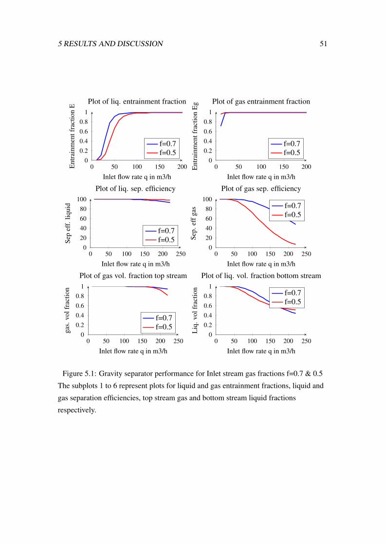
The Matlab code for this separator mod_grav.m is attached to Appendix A.1.2. The
figure 5.1 below shows the model results obtained for inlet gas fractions of 0.7 and 0.5.
It is seen from the figure that Entrainment fractions of each dispersed phase in a contin-
uous one increase with increasing inlet flow rate because increased flow rates result in
increased velocities thus phase dispersion increases, resulting into higher entrainment
fractions.
In addition, the separation efficiencies also decrease with increasing flow rates. For
example, for the liquid phase, as the inlet flow rate increases, the gas velocity increases
outweighing the liquid terminal velocity. This liquid is thus carried with the top gas
stream resulting in lower gas volume fractions of the top outlet stream. Also as the
liquid separation efficiency decreases, more liquid remains entrained in the gas stream
resulting in lower gas fractions.
A similar scenario occurs for the gas phase in which case an increase in inlet flow
rates results in higher liquid velocities. Thus the gas rise velocities become smaller
in comparison to liquid velocities and more gas is carried by the outlet bottom stream
resulting in lower separation efficiencies and lower liquid volume fractions.
The above arguments are in agreement with the analysis and results by Bothamley et al.
(2013a), who reports that higher inlet momentum rates (higher feed pipe velocities)
result in higher entrainment loads, smaller droplet sizes and more difficult separation
conditions.
It can also been seen from the model predictions in figure 5.1 that a decrease of the inlet
gas volume fraction from 0.7 to 0.5 for the same conditions results in an decrease in
liquid entrainment and higher liquid separation efficiency. However, gas entrainment in
liquid increases resulting in lower gas separation efficiency and therefore the top stream
gas volume fraction decreases. In addition the bottom stream liquid volume fraction
5 RESULTS AND DISCUSSION 51
0 50 100 150 2000
0.20.40.6
0.81
Inlet flow rate q in m3/h
Ent
rain
men
tfra
ctio
nE
Plot of liq. entrainment fraction
f=0.7f=0.5
0 50 100 150 2000
0.20.40.6
0.81
Inlet flow rate q in m3/h
Ent
rain
men
tfra
ctio
nE
g Plot of gas entrainment fraction
f=0.7f=0.5
0 50 100 150 200 2500
204060
80100
Inlet flow rate q in m3/h
Sep.
effg
asPlot of gas sep. efficiency
f=0.7f=0.5
0 50 100 150 200 2500
204060
80100
Inlet flow rate q in m3/h
Sep
eff.
liqui
d
Plot of liq. sep. efficiency
f=0.7f=0.5
0 50 100 150 200 2500
0.20.40.6
0.81
Inlet flow rate q in m3/h
Liq
.vol
frac
tion
Plot of liq. vol. fraction bottom stream
f=0.7f=0.5
0 50 100 150 200 2500
0.20.40.6
0.81
Inlet flow rate q in m3/h
gas.
volf
ract
ion
Plot of gas vol. fraction top stream
f=0.7f=0.5
Figure 5.1: Gravity separator performance for Inlet stream gas fractions f=0.7 & 0.5
The subplots 1 to 6 represent plots for liquid and gas entrainment fractions, liquid and
gas separation efficiencies, top stream gas and bottom stream liquid fractions
respectively.
5 RESULTS AND DISCUSSION 52
also decreases because of increased gas content.
5.1.2 Deliquidizer
The Matlab code for this separator mod_deliq.m is attached to Appendix A.1.3. The
results obtained for this separator are shown in figure 5.2 below.
At low inlet flow rates, the swirl intensities generated are low resulting in low angular
velocities and low radial velocities. This results in low centrifugal forces which are
desired for phase separation and hence low liquid separation efficiencies.
An increase in inlet flow rate results in increased angular velocities and ultimately in-
creased separation forces. Therefore, the liquid separation efficiency increases. This
decreases the amount of liquid in the gas stream thus the gas volume fraction of the
top stream also increases as shown in sub-plot 3. Also, since more liquid is separated,
the amount of liquid in the bottom stream increases thus increasing the bottom stream
liquid volume fraction.
Further increase in the inlet flow rate results in a levelling off of the angular velocity as is
predicted by the gompertz function used (see subsection 3.2.1). This function was tested
against experimental data during the Specialization Project course in spring 2015 and
shown to produce better model predictions. The levelling off has in this work been used
to cater for mixing of already separated phases (re-entrainment) that would be expected
at very high flow rates. The increase in inlet flow rate results in a decrease in droplet
axial time and no further increase in droplet radial time because the angular velocity
levels off. Therefore the liquid separation efficiency starts decreasing as is shown in
sub-plot 2.
This decrease in separation efficiency translates to more liquid in the gas hence the gas
volume fraction also decreases. In addition, the bottom stream liquid volume fraction
also decreases because less liquid is separated from the gas.
For the same conditions and constant inlet flow rate, a decrease in split fraction from
0.85 to 0.7 does not affect both the angular velocity and liquid separation efficiency as is
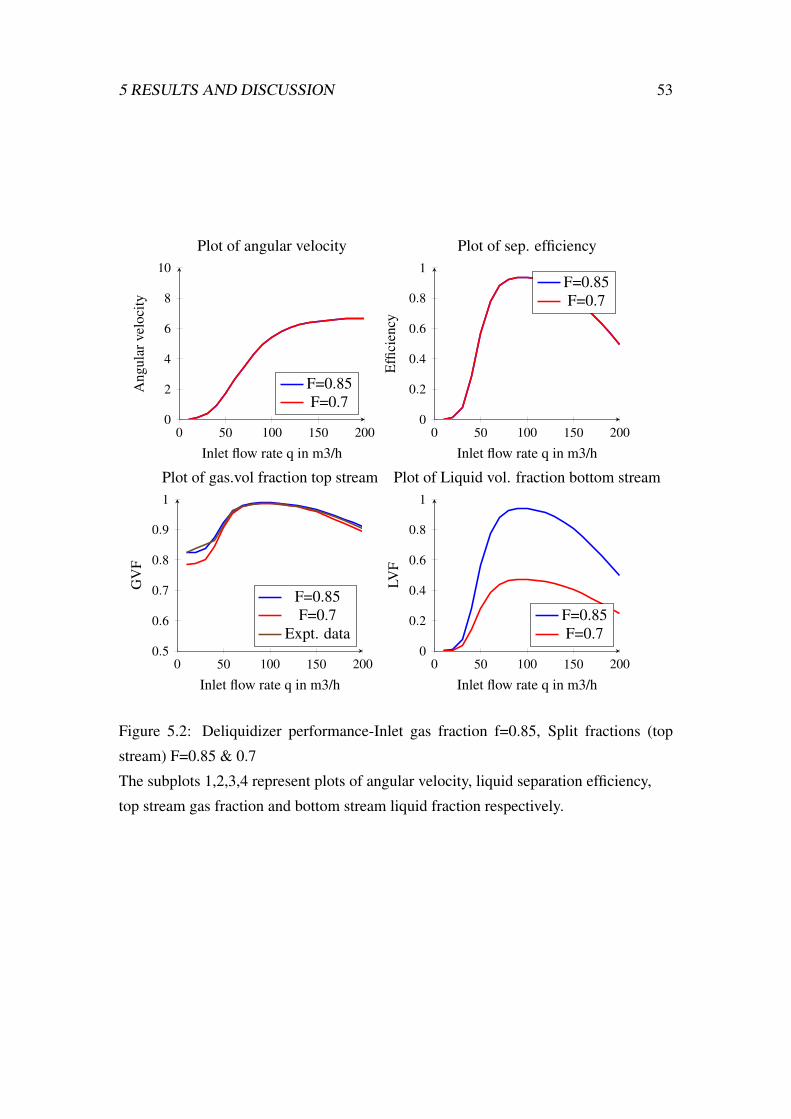
5 RESULTS AND DISCUSSION 53
0 50 100 150 2000
2
4
6
8
10
Inlet flow rate q in m3/h
Ang
ular
velo
city
Plot of angular velocity
F=0.85F=0.7
0 50 100 150 2000
0.2
0.4
0.6
0.8
1
Inlet flow rate q in m3/h
Effi
cien
cy
Plot of sep. efficiency
F=0.85F=0.7
0 50 100 150 2000
0.2
0.4
0.6
0.8
1
Inlet flow rate q in m3/h
LVF
Plot of Liquid vol. fraction bottom stream
F=0.85F=0.7
0 50 100 150 2000.5
0.6
0.7
0.8
0.9
1
Inlet flow rate q in m3/h
GV
F
Plot of gas.vol fraction top stream
F=0.85F=0.7
Expt. data
Figure 5.2: Deliquidizer performance-Inlet gas fraction f=0.85, Split fractions (top
stream) F=0.85 & 0.7
The subplots 1,2,3,4 represent plots of angular velocity, liquid separation efficiency,
top stream gas fraction and bottom stream liquid fraction respectively.
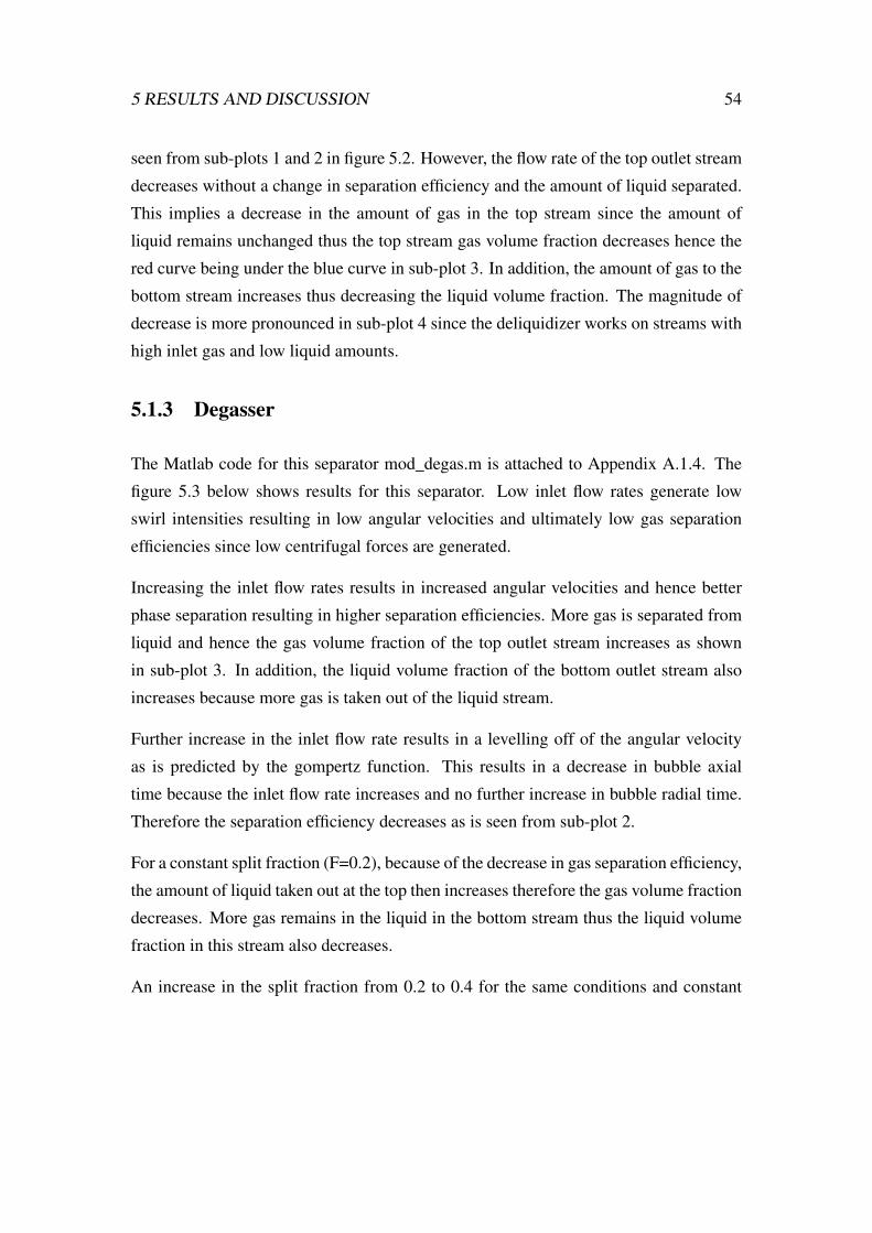
5 RESULTS AND DISCUSSION 54
seen from sub-plots 1 and 2 in figure 5.2. However, the flow rate of the top outlet stream
decreases without a change in separation efficiency and the amount of liquid separated.
This implies a decrease in the amount of gas in the top stream since the amount of
liquid remains unchanged thus the top stream gas volume fraction decreases hence the
red curve being under the blue curve in sub-plot 3. In addition, the amount of gas to the
bottom stream increases thus decreasing the liquid volume fraction. The magnitude of
decrease is more pronounced in sub-plot 4 since the deliquidizer works on streams with
high inlet gas and low liquid amounts.
5.1.3 Degasser
The Matlab code for this separator mod_degas.m is attached to Appendix A.1.4. The
figure 5.3 below shows results for this separator. Low inlet flow rates generate low
swirl intensities resulting in low angular velocities and ultimately low gas separation
efficiencies since low centrifugal forces are generated.
Increasing the inlet flow rates results in increased angular velocities and hence better
phase separation resulting in higher separation efficiencies. More gas is separated from
liquid and hence the gas volume fraction of the top outlet stream increases as shown
in sub-plot 3. In addition, the liquid volume fraction of the bottom outlet stream also
increases because more gas is taken out of the liquid stream.
Further increase in the inlet flow rate results in a levelling off of the angular velocity
as is predicted by the gompertz function. This results in a decrease in bubble axial
time because the inlet flow rate increases and no further increase in bubble radial time.
Therefore the separation efficiency decreases as is seen from sub-plot 2.
For a constant split fraction (F=0.2), because of the decrease in gas separation efficiency,
the amount of liquid taken out at the top then increases therefore the gas volume fraction
decreases. More gas remains in the liquid in the bottom stream thus the liquid volume
fraction in this stream also decreases.
An increase in the split fraction from 0.2 to 0.4 for the same conditions and constant
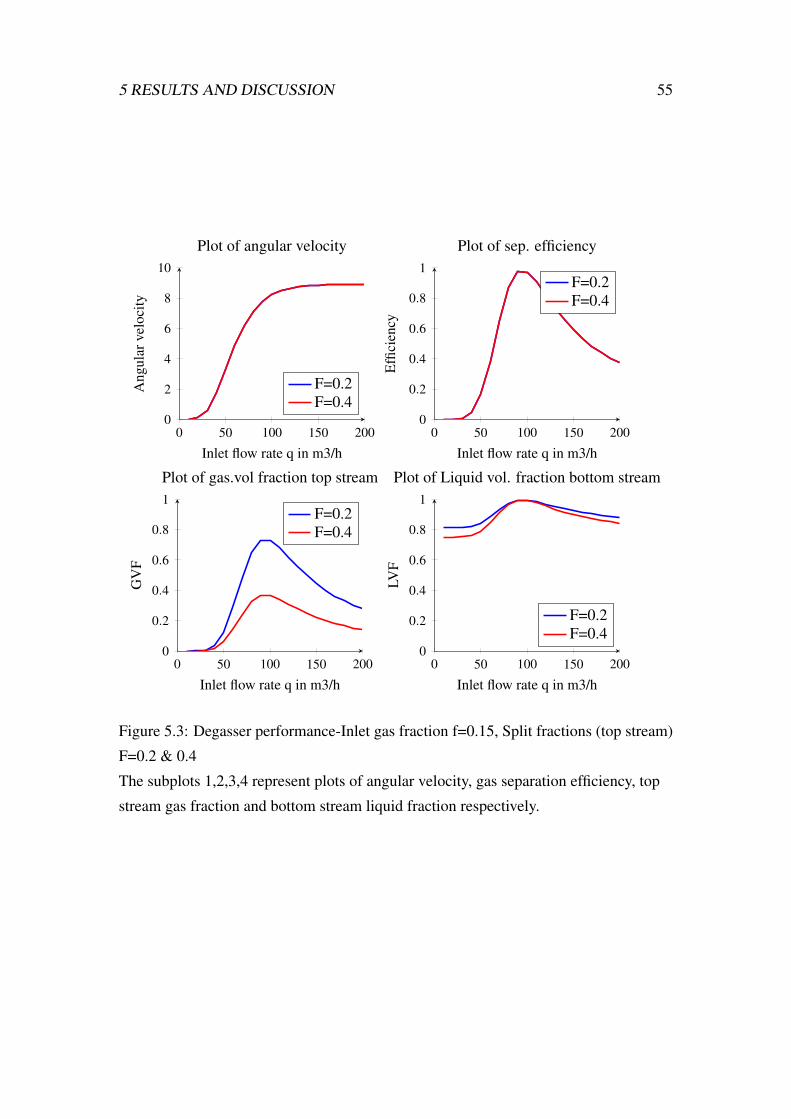
5 RESULTS AND DISCUSSION 55
0 50 100 150 2000
2
4
6
8
10
Inlet flow rate q in m3/h
Ang
ular
velo
city
Plot of angular velocity
F=0.2F=0.4
0 50 100 150 2000
0.2
0.4
0.6
0.8
1
Inlet flow rate q in m3/h
Effi
cien
cy
Plot of sep. efficiency
F=0.2F=0.4
0 50 100 150 2000
0.2
0.4
0.6
0.8
1
Inlet flow rate q in m3/h
LVF
Plot of Liquid vol. fraction bottom stream
F=0.2F=0.4
0 50 100 150 2000
0.2
0.4
0.6
0.8
1
Inlet flow rate q in m3/h
GV
F
Plot of gas.vol fraction top stream
F=0.2F=0.4
Figure 5.3: Degasser performance-Inlet gas fraction f=0.15, Split fractions (top stream)
F=0.2 & 0.4
The subplots 1,2,3,4 represent plots of angular velocity, gas separation efficiency, top
stream gas fraction and bottom stream liquid fraction respectively.
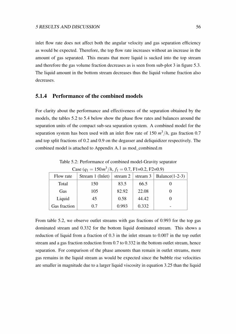
5 RESULTS AND DISCUSSION 56
inlet flow rate does not affect both the angular velocity and gas separation efficiency
as would be expected. Therefore, the top flow rate increases without an increase in the
amount of gas separated. This means that more liquid is sucked into the top stream
and therefore the gas volume fraction decreases as is seen from sub-plot 3 in figure 5.3.
The liquid amount in the bottom stream decreases thus the liquid volume fraction also
decreases.
5.1.4 Performance of the combined models
For clarity about the performance and effectiveness of the separation obtained by the
models, the tables 5.2 to 5.4 below show the phase flow rates and balances around the
separation units of the compact sub-sea separation system. A combined model for the
separation system has been used with an inlet flow rate of 150 m3/h, gas fraction 0.7
and top split fractions of 0.2 and 0.9 on the degasser and deliquidizer respectively. The
combined model is attached to Appendix A.1 as mod_combined.m
Table 5.2: Performance of combined model-Gravity separator
Case (q1 = 150m3/h, f1 = 0.7, F1=0.2, F2=0.9)Flow rate Stream 1 (Inlet) stream 2 stream 3 Balance(1-2-3)
Total 150 83.5 66.5 0
Gas 105 82.92 22.08 0
Liquid 45 0.58 44.42 0
Gas fraction 0.7 0.993 0.332 -
From table 5.2, we observe outlet streams with gas fractions of 0.993 for the top gas
dominated stream and 0.332 for the bottom liquid dominated stream. This shows a
reduction of liquid from a fraction of 0.3 in the inlet stream to 0.007 in the top outlet
stream and a gas fraction reduction from 0.7 to 0.332 in the bottom outlet stream, hence
separation. For comparison of the phase amounts than remain in outlet streams, more
gas remains in the liquid stream as would be expected since the bubble rise velocities
are smaller in magnitude due to a larger liquid viscosity in equation 3.25 than the liquid
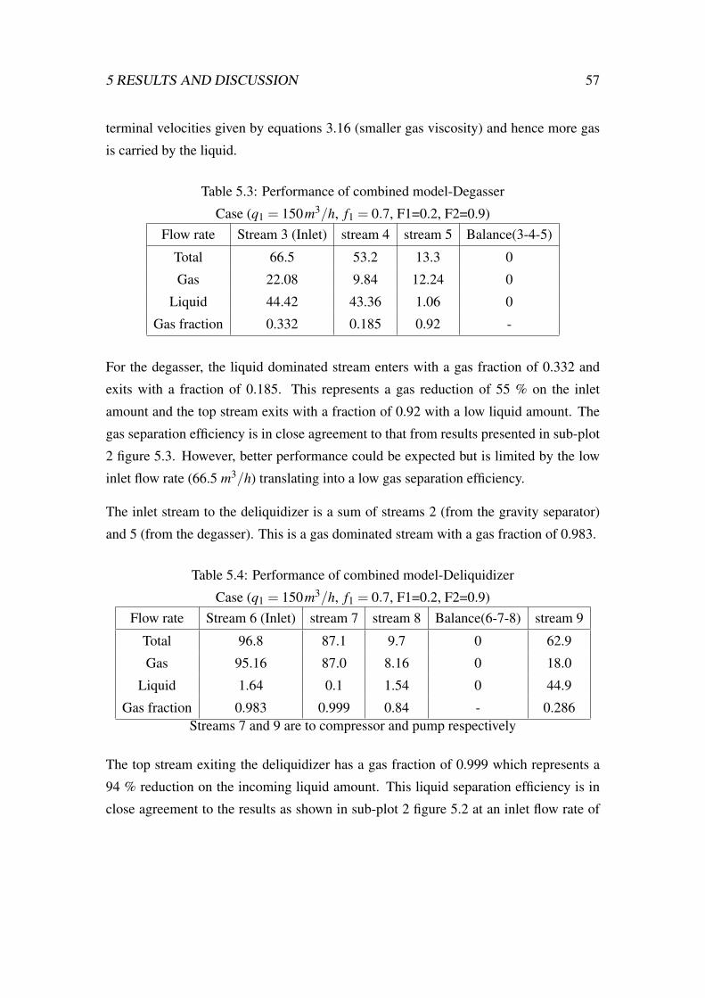
5 RESULTS AND DISCUSSION 57
terminal velocities given by equations 3.16 (smaller gas viscosity) and hence more gas
is carried by the liquid.
Table 5.3: Performance of combined model-Degasser
Case (q1 = 150m3/h, f1 = 0.7, F1=0.2, F2=0.9)Flow rate Stream 3 (Inlet) stream 4 stream 5 Balance(3-4-5)
Total 66.5 53.2 13.3 0
Gas 22.08 9.84 12.24 0
Liquid 44.42 43.36 1.06 0
Gas fraction 0.332 0.185 0.92 -
For the degasser, the liquid dominated stream enters with a gas fraction of 0.332 and
exits with a fraction of 0.185. This represents a gas reduction of 55 % on the inlet
amount and the top stream exits with a fraction of 0.92 with a low liquid amount. The
gas separation efficiency is in close agreement to that from results presented in sub-plot
2 figure 5.3. However, better performance could be expected but is limited by the low
inlet flow rate (66.5 m3/h) translating into a low gas separation efficiency.
The inlet stream to the deliquidizer is a sum of streams 2 (from the gravity separator)
and 5 (from the degasser). This is a gas dominated stream with a gas fraction of 0.983.
Table 5.4: Performance of combined model-Deliquidizer
Case (q1 = 150m3/h, f1 = 0.7, F1=0.2, F2=0.9)Flow rate Stream 6 (Inlet) stream 7 stream 8 Balance(6-7-8) stream 9
Total 96.8 87.1 9.7 0 62.9
Gas 95.16 87.0 8.16 0 18.0
Liquid 1.64 0.1 1.54 0 44.9
Gas fraction 0.983 0.999 0.84 - 0.286Streams 7 and 9 are to compressor and pump respectively
The top stream exiting the deliquidizer has a gas fraction of 0.999 which represents a
94 % reduction on the incoming liquid amount. This liquid separation efficiency is in
close agreement to the results as shown in sub-plot 2 figure 5.2 at an inlet flow rate of
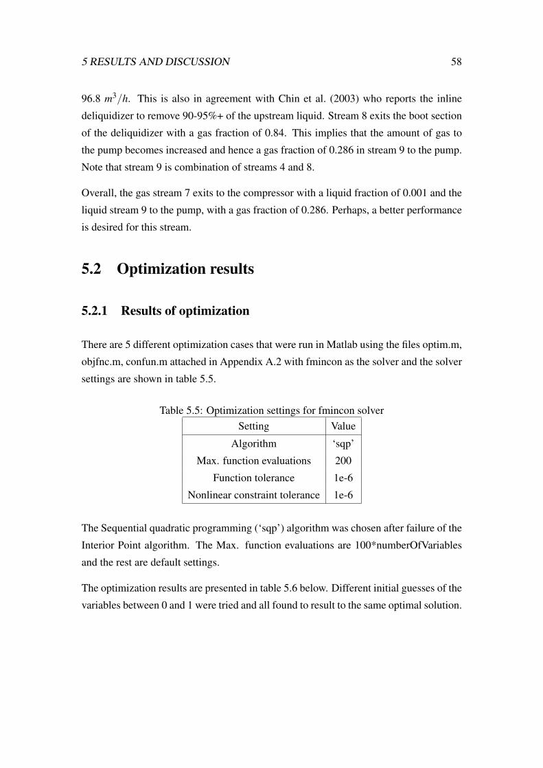
5 RESULTS AND DISCUSSION 58
96.8 m3/h. This is also in agreement with Chin et al. (2003) who reports the inline
deliquidizer to remove 90-95%+ of the upstream liquid. Stream 8 exits the boot section
of the deliquidizer with a gas fraction of 0.84. This implies that the amount of gas to
the pump becomes increased and hence a gas fraction of 0.286 in stream 9 to the pump.
Note that stream 9 is combination of streams 4 and 8.
Overall, the gas stream 7 exits to the compressor with a liquid fraction of 0.001 and the
liquid stream 9 to the pump, with a gas fraction of 0.286. Perhaps, a better performance
is desired for this stream.
5.2 Optimization results
5.2.1 Results of optimization
There are 5 different optimization cases that were run in Matlab using the files optim.m,
objfnc.m, confun.m attached in Appendix A.2 with fmincon as the solver and the solver
settings are shown in table 5.5.
Table 5.5: Optimization settings for fmincon solverSetting Value
Algorithm ‘sqp’
Max. function evaluations 200
Function tolerance 1e-6
Nonlinear constraint tolerance 1e-6
The Sequential quadratic programming (‘sqp’) algorithm was chosen after failure of the
Interior Point algorithm. The Max. function evaluations are 100*numberOfVariables
and the rest are default settings.
The optimization results are presented in table 5.6 below. Different initial guesses of the
variables between 0 and 1 were tried and all found to result to the same optimal solution.
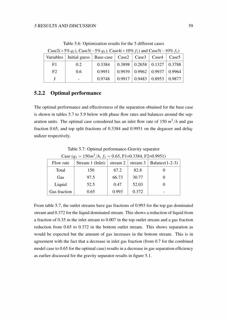
5 RESULTS AND DISCUSSION 59
Table 5.6: Optimization results for the 5 different cases
Case2(+5%q1), Case3(−5%q1), Case4(+10% f1) and Case5(−10% f1)Variables Initial guess Base-case Case2 Case3 Case4 Case5
F1 0.2 0.3384 0.3898 0.2658 0.1327 0.3788
F2 0.6 0.9951 0.9939 0.9962 0.9937 0.9964
J - 0.9748 0.9917 0.9483 0.8953 0.9877
5.2.2 Optimal performance
The optimal performance and effectiveness of the separation obtained for the base case
is shown in tables 5.7 to 5.9 below with phase flow rates and balances around the sep-
aration units. The optimal case considered has an inlet flow rate of 150 m3/h and gas
fraction 0.65, and top split fractions of 0.3384 and 0.9951 on the degasser and deliq-
uidizer respectively.
Table 5.7: Optimal performance-Gravity separator
Case (q1 = 150m3/h, f1 = 0.65, F1=0.3384, F2=0.9951)Flow rate Stream 1 (Inlet) stream 2 stream 3 Balance(1-2-3)
Total 150 67.2 82.8 0
Gas 97.5 66.73 30.77 0
Liquid 52.5 0.47 52.03 0
Gas fraction 0.65 0.993 0.372 -
From table 5.7, the outlet streams have gas fractions of 0.993 for the top gas dominated
stream and 0.372 for the liquid dominated stream. This shows a reduction of liquid from
a fraction of 0.35 in the inlet stream to 0.007 in the top outlet stream and a gas fraction
reduction from 0.65 to 0.372 in the bottom outlet stream. This shows separation as
would be expected but the amount of gas increases in the bottom stream. This is in
agreement with the fact that a decrease in inlet gas fraction (from 0.7 for the combined
model case to 0.65 for the optimal case) results in a decrease in gas separation efficiency
as earlier discussed for the gravity separator results in figure 5.1.
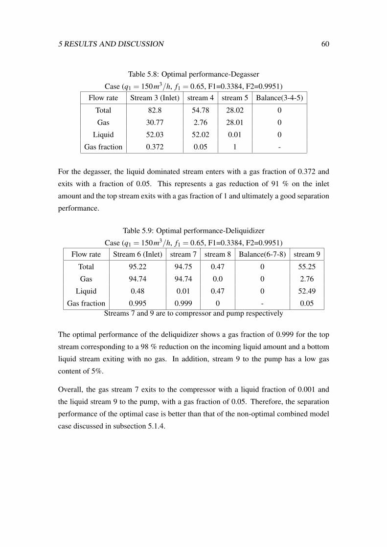
5 RESULTS AND DISCUSSION 60
Table 5.8: Optimal performance-Degasser
Case (q1 = 150m3/h, f1 = 0.65, F1=0.3384, F2=0.9951)Flow rate Stream 3 (Inlet) stream 4 stream 5 Balance(3-4-5)
Total 82.8 54.78 28.02 0
Gas 30.77 2.76 28.01 0
Liquid 52.03 52.02 0.01 0
Gas fraction 0.372 0.05 1 -
For the degasser, the liquid dominated stream enters with a gas fraction of 0.372 and
exits with a fraction of 0.05. This represents a gas reduction of 91 % on the inlet
amount and the top stream exits with a gas fraction of 1 and ultimately a good separation
performance.
Table 5.9: Optimal performance-Deliquidizer
Case (q1 = 150m3/h, f1 = 0.65, F1=0.3384, F2=0.9951)Flow rate Stream 6 (Inlet) stream 7 stream 8 Balance(6-7-8) stream 9
Total 95.22 94.75 0.47 0 55.25
Gas 94.74 94.74 0.0 0 2.76
Liquid 0.48 0.01 0.47 0 52.49
Gas fraction 0.995 0.999 0 - 0.05Streams 7 and 9 are to compressor and pump respectively
The optimal performance of the deliquidizer shows a gas fraction of 0.999 for the top
stream corresponding to a 98 % reduction on the incoming liquid amount and a bottom
liquid stream exiting with no gas. In addition, stream 9 to the pump has a low gas
content of 5%.
Overall, the gas stream 7 exits to the compressor with a liquid fraction of 0.001 and
the liquid stream 9 to the pump, with a gas fraction of 0.05. Therefore, the separation
performance of the optimal case is better than that of the non-optimal combined model
case discussed in subsection 5.1.4.
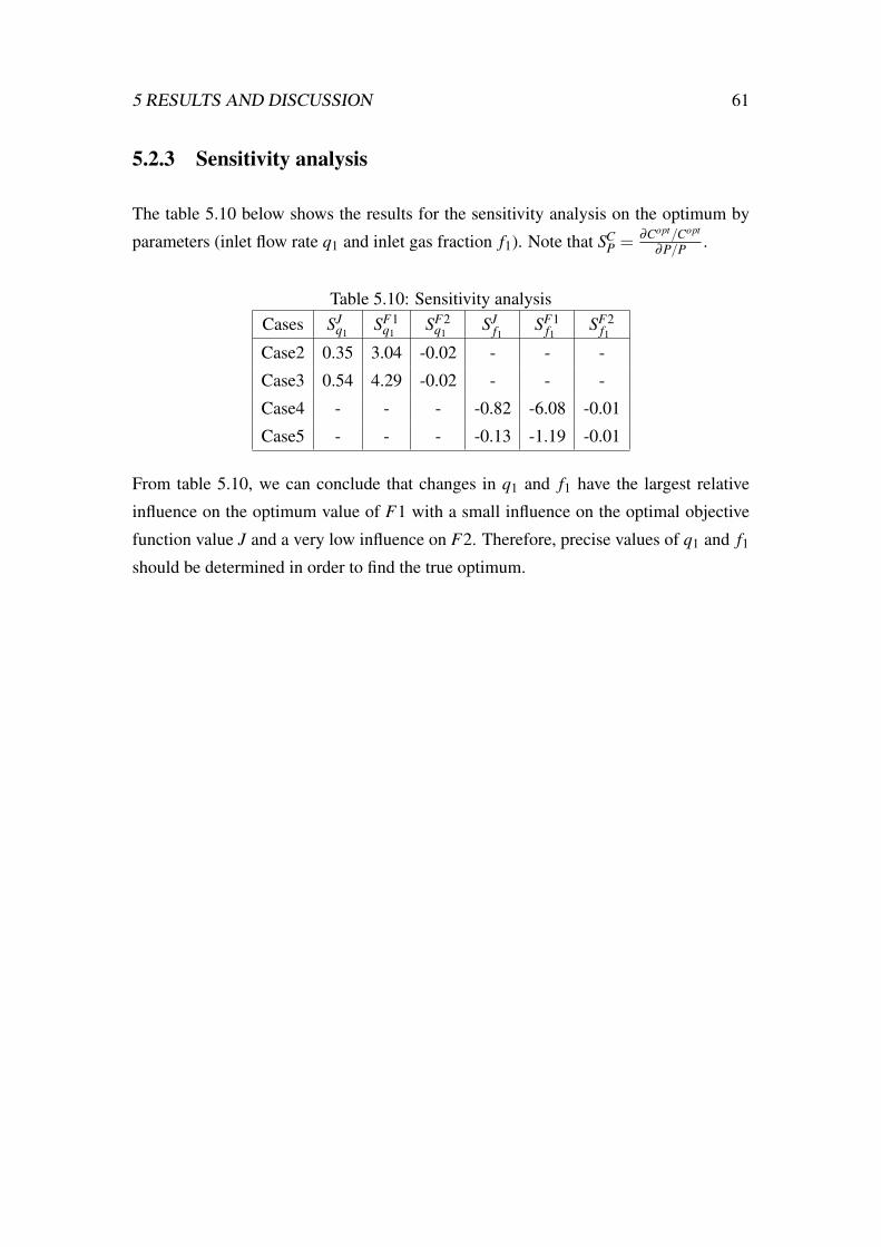
5 RESULTS AND DISCUSSION 61
5.2.3 Sensitivity analysis
The table 5.10 below shows the results for the sensitivity analysis on the optimum by
parameters (inlet flow rate q1 and inlet gas fraction f1). Note that SCP = ∂Copt/Copt
∂P/P .
Table 5.10: Sensitivity analysisCases SJ
q1SF1
q1SF2
q1SJ
f1 SF1f1 SF2
f1
Case2 0.35 3.04 -0.02 - - -
Case3 0.54 4.29 -0.02 - - -
Case4 - - - -0.82 -6.08 -0.01
Case5 - - - -0.13 -1.19 -0.01
From table 5.10, we can conclude that changes in q1 and f1 have the largest relative
influence on the optimum value of F1 with a small influence on the optimal objective
function value J and a very low influence on F2. Therefore, precise values of q1 and f1
should be determined in order to find the true optimum.
6 CONCLUSION AND FUTURE WORK 62
6 Conclusion and Future work
6.1 Conclusion
The steady state models developed for the separation units of the compact sub-sea sep-
aration system have been shown to predict phase separation between gas and liquid
phases and output stream flow rates and phase fractions. The trends of model results
obtained are consistent with theoretical expectations.
Optimization on the system has been carried out and the results obtained have shown an
average of not more than 5% of the dispersed phase in exit streams to the compressor
and pump.
However, the lack of experimental data for the compact sub-sea separation system has
been a major short coming in the validation of simulation results.
6.2 Future work
The models developed in this thesis do not account for the different flow regimes that
are encountered for two-phase flow but assume a uniform regime of either annular or
bubble flow. Therefore, the possibility of other regimes should later be considered.
We have assumed uniform droplet/ bubble size distributions for both the deliquidizer
and degasser. However, the use of upper limit log normal distribution as used for the
gravity separator may be considered in future work.
The gompertz function has been used in this report to represent angular velocity/ fre-
quency in cyclonic separators. However, further studies about this representation should
be considered.
We have assumed forced vortex flow in this thesis which is a good assumption only at
the inlet but experimental studies have shown a combined vortex as the vortex associated
6 CONCLUSION AND FUTURE WORK 63
with cyclonic separation and should therefore be considered.
In addition, the strength of swirling flow decays along the cyclone length but this has
not been considered in our model representations.
The validation of the model results presented in this thesis has been let down by the lack
of experimental data. Thus, there is need to carry out experimental studies about the
performance of these separation units.
BIBLIOGRAPHY 64
Bibliography
Alary, V., Marchais, F., Palermo, T., et al., 2000. Subsea water separation and injection:
A solution for hydrates. In: Offshore Technology Conference. Offshore Technology
Conference.
Arpandi, I., Joshi, A., Shoham, O., Shirazi, S., Kouba, G., et al., 1996. Hydrodynamics
of two-phase flow in gas-liquid cylindrical cyclone separators. SPE Journal 1 (04),
427–436.
Arpandi, I. A., 1995. A mechanistic model for two-phase flow in gas-liquid cylindrical
cyclone separators. Ph.D. thesis, University of Tulsa.
Bothamley, M., et al., 2013a. Gas/liquid separators:quantifying separation performance-
part 1. Oil and Gas Facilities 2 (04), 21–29.
Bothamley, M., et al., 2013b. Gas/liquid separators:quantifying separation performance-
part 2. Oil and Gas Facilities 2 (05), 35–47.
Brenne, L., BjoÌÿrge, T., Bakken, L. E., Hundseid, O., 2008. Prospects for sub sea
wet gas compression. In: ASME Turbo Expo 2008: Power for Land, Sea, and Air.
American Society of Mechanical Engineers, pp. 671–677.
Chin, R., Stanbridg, D., Schook, R., et al., 2003. Development and installation of an
inline deliquidiser. In: SPE Annual Technical Conference and Exhibition. Society of
Petroleum Engineers.
Edgar, T. F., Himmelblau, D. M., Lasdon, L., 1989. Optimization of chemical processes.
McGraw-Hill.
Ellingsen, C., 2007. Compact sub sea separation: Implementation and comparison of
two different control structures. Master’s thesis, Norwegian University of Science
and Technology.
BIBLIOGRAPHY 65
FMCtechnologies, February 2011. Compact total separation systems.
URL www.fmctechnologies.com/separation
Gomez, L., Mohan, R., Shoham, O., Kouba, G., et al., 2000. Enhanced mechanistic
model and field-application design of gas/liquid cylindrical cyclone separators. Spe
Journal 5 (02), 190–198.
Hamoud, A. A., Boudi, A. A., Al-Qahtani, S. D., 2009. New application of an inline sep-
aration technology in a real wet gas field. SAUDI ARAMCO JOURNAL OF TECH-
NOLOGY, 41.
Hinze, J., 1955. Fundamentals of the hydrodynamic mechanism of splitting in disper-
sion processes. AIChE Journal 1 (3), 289–295.
Hoffmann, A. C., Stein, L. E., 2002. Gas cyclones and swirl tubes. Springer-Verlag
Berlin Heidelberg 2008.
Kataoka, I., Ishii, M., Mishima, K., 1983. Generation and size distribution of droplet in
annular two-phase flow. Journal of Fluids Engineering 105 (2), 230–238.
Kouba, G., Shoham, O., 1996. A review of gas-liquid cylindrical cyclone (glcc) tech-
nology. In: Production Separation Systems International Conference, Aberdeen, Eng-
land, April. pp. 23–24.
Kouba, G. E., Shoham, O., Shirazi, S., 1995. Design and performance of gas-liquid
cylindrical cyclone separators. In: Proceedings of the BHR Group 7th International
Meeting on Multiphase Flow, Cannes, France. pp. 307–327.
Marti, S., Erdal, F., Shoham, O., Shirazi, S., Kouba, G., 1996. Analysis of gas carry-
under in gas-liquid cylindrical cyclones. In: Hydrocyclones 1996 International Meet-
ing, St. John College, Cambridge, England, April. pp. 2–4.
Mokhatab, S., Poe, W. A., 2012. Handbook of natural gas transmission and processing.
Gulf Professional Publishing.
BIBLIOGRAPHY 66
Monsen, G. O. T., 2012. Modeling of a centrifugal separator for dispersed gas-liquid
flows.
Movafaghian, S., Jaua-Marturet, J., Mohan, R. S., Shoham, O., Kouba, G., 2000. The
effects of geometry, fluid properties and pressure on the hydrodynamics of gas–liquid
cylindrical cyclone separators. International Journal of Multiphase Flow 26 (6), 999–
1018.
Pan, L., Hanratty, T. J., 2002. Correlation of entrainment for annular flow in horizontal
pipes. International journal of multiphase flow 28 (3), 385–408.
Pereyra, E., Gomez, L., Mohan, R., Shoham, O., Kouba, G., 2009. Transient mechanis-
tic model for slug damper/gas-liquid cylindrical cyclone (glcc©) compact separator
system. In: ASME 2009 28th International Conference on Ocean, Offshore and Arc-
tic Engineering. American Society of Mechanical Engineers, pp. 661–672.
Rangaiah, G. P., Kariwala, V., 2012. Plantwide control: Recent developments and ap-
plications. John Wiley & Sons.
Sayda, A. F., Taylor, J. H., 2007. Modeling and control of three-phase gravilty separators
in oil production facilities. In: American Control Conference, 2007. ACC’07. IEEE,
pp. 4847–4853.
Schook, R., van Vorselen, M., et al., 2005. Compact separation by means of inline tech-
nology. In: Offshore Mediterranean Conference and Exhibition. Offshore Mediter-
ranean Conference.
Simmons, M. J., Hanratty, T. J., 2001. Droplet size measurements in horizontal annular
gas–liquid flow. International journal of multiphase flow 27 (5), 861–883.
Skogestad, S., 2004. Near-optimal operation by self-optimizing control: From process
control to marathon running and business systems. Computers & chemical engineer-
ing 29 (1), 127–137.
Stene, M., 2013. Cfd study of a rotating gas-liquid separator: Design og bygging av
flere mikro-dråpe generatorer.
BIBLIOGRAPHY 67
Swanborn, R. A., 1988. A new approach to the design of gas-liquid separators for the
oil industry. Univerity of Delft.
Van Campen, L., 2014. Bulk dynamics of droplets in liquid-liquid axial cyclones. Ph.D.
thesis, TU Delft, Delft University of Technology.
van Wissen, R., Brouwers, J., Golombok, M., 2007. In-line centrifugal separation of
dispersed phases. AIChE journal 53 (2), 374–380.
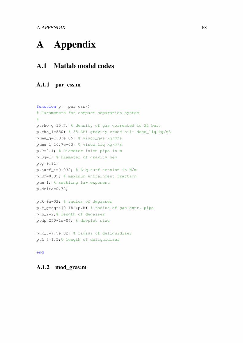
A APPENDIX 68
A Appendix
A.1 Matlab model codes
A.1.1 par_css.m
function p = par_css()
% Parameters for compact separation system
%
p.rho_g=15.7; % density of gas corrected to 25 bar.
p.rho_l=850; % 35 API gravity crude oil- dens_liq kg/m3
p.mu_g=1.83e-05; % visco_gas kg/m/s
p.mu_l=16.7e-03; % visco_liq kg/m/s
p.D=0.1; % Diameter inlet pipe in m
p.Dg=1; % Diameter of gravity sep
p.g=9.81;
p.surf_t=0.032; % Liq surf tension in N/m
p.Em=0.99; % maximum entrainment fraction
p.m=1; % settling law exponent
p.delta=0.72;
p.R=9e-02; % radius of degasser
p.r_g=sqrt(0.18)*p.R; % radius of gas extr. pipe
p.L_2=2;% length of degasser
p.dp=250*1e-06; % droplet size
p.R_3=7.5e-02; % radius of deliquidizer
p.L_3=1.5;% length of deliquidizer
end
A.1.2 mod_grav.m
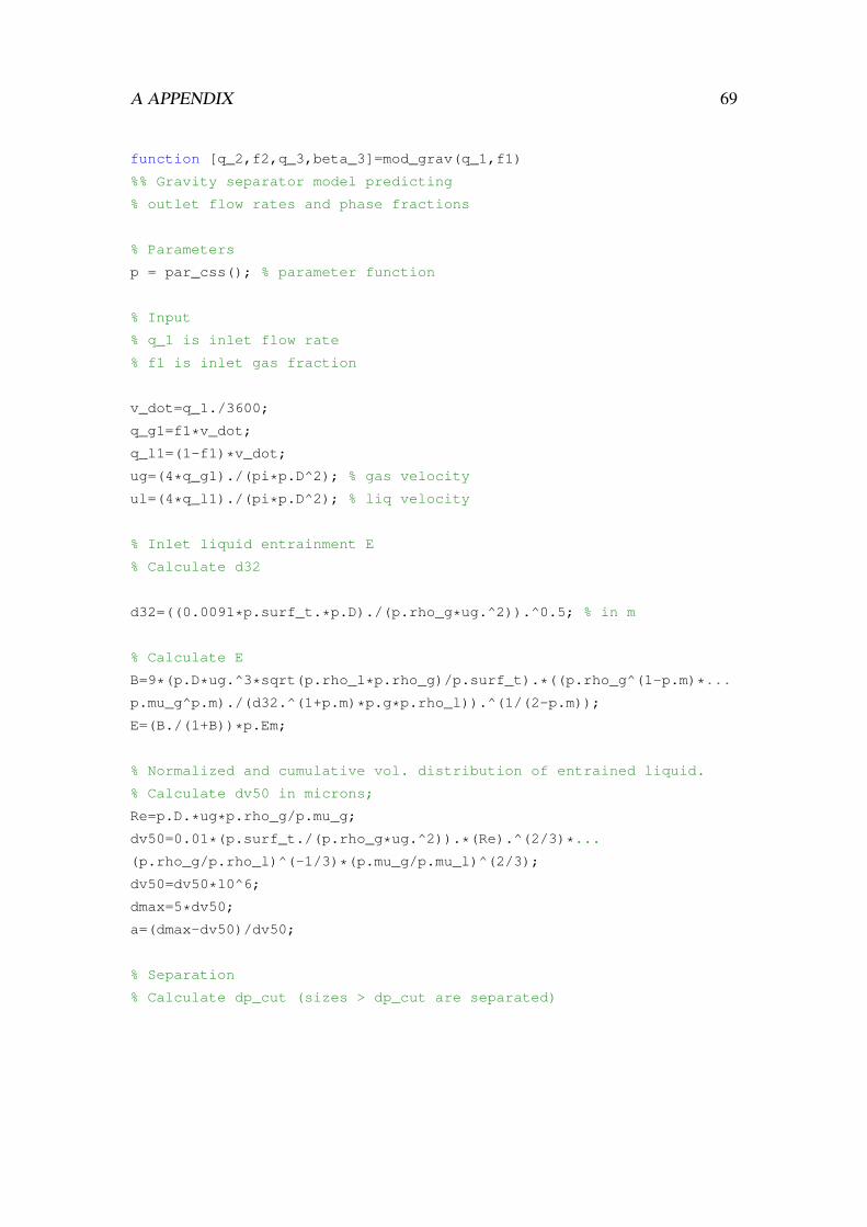
A APPENDIX 69
function [q_2,f2,q_3,beta_3]=mod_grav(q_1,f1)
%% Gravity separator model predicting
% outlet flow rates and phase fractions
% Parameters
p = par_css(); % parameter function
% Input
% q_1 is inlet flow rate
% f1 is inlet gas fraction
v_dot=q_1./3600;
q_g1=f1*v_dot;
q_l1=(1-f1)*v_dot;
ug=(4*q_g1)./(pi*p.D^2); % gas velocity
ul=(4*q_l1)./(pi*p.D^2); % liq velocity
% Inlet liquid entrainment E
% Calculate d32
d32=((0.0091*p.surf_t.*p.D)./(p.rho_g*ug.^2)).^0.5; % in m
% Calculate E
B=9*(p.D*ug.^3*sqrt(p.rho_l*p.rho_g)/p.surf_t).*((p.rho_g^(1-p.m)*...
p.mu_g^p.m)./(d32.^(1+p.m)*p.g*p.rho_l)).^(1/(2-p.m));
E=(B./(1+B))*p.Em;
% Normalized and cumulative vol. distribution of entrained liquid.
% Calculate dv50 in microns;
Re=p.D.*ug*p.rho_g/p.mu_g;
dv50=0.01*(p.surf_t./(p.rho_g*ug.^2)).*(Re).^(2/3)*...
(p.rho_g/p.rho_l)^(-1/3)*(p.mu_g/p.mu_l)^(2/3);
dv50=dv50*10^6;
dmax=5*dv50;
a=(dmax-dv50)/dv50;
% Separation
% Calculate dp_cut (sizes > dp_cut are separated)
A APPENDIX 70
% Equating the terminal droplet and gas velocities
dp_cut=((4*18*p.mu_g*q_g1)./(pi*p.Dg^2*p.g*(p.rho_l-p.rho_g)))...
.^0.5*10^6;
z_cut=log(a.*dp_cut./(dmax-dp_cut));
Beta=1-0.5*(1-erf(p.delta*z_cut)); % Fract.entrained liq in exit gas
% Sep. efficiency liq
sep_eff=(1-Beta)*100;
%% Gas entrainment
% Calculate d32g
d32g=((0.0091*p.surf_t.*p.D)./(p.rho_l*ul.^2)).^0.5; % in m
% Calculate Eg
Bg=9*(p.D*ul.^3*sqrt(p.rho_l*p.rho_g)/p.surf_t).*((p.rho_l^...
(1-p.m)*p.mu_l^p.m)./(d32g.^(1+p.m)*p.g*p.rho_l)).^(1/(2-p.m));
Eg=(Bg./(1+Bg))*p.Em;
% Normalized and cumulative vol. distribution of entrained gas.
Reg=p.D.*ul*p.rho_l/p.mu_l;
dv50g=0.01*(p.surf_t./(p.rho_l*ul.^2)).*(Reg).^(2/3)*...
(p.rho_l/p.rho_g)^(-1/3)*(p.mu_l/p.mu_g)^(2/3);
dv50g=dv50g*10^6;
dmaxg=5*dv50g;
ag=(dmaxg-dv50g)/dv50g;
% Separation
dp_cutg=((4*18*p.mu_l*q_l1)./(pi*p.Dg^2*p.g*(p.rho_l-p.rho_g)))...
.^0.5*10^6;
z_cutg=log(ag.*dp_cutg./(dmaxg-dp_cutg));
Betag=1-0.5*(1-erf(p.delta*z_cutg));
% Sep. efficiency gas
sep_effg=(1-Betag)*100;
% Exiting stream flow rates and fractions
q_l2=Beta.*E.*(1-f1).*q_1; % liq out top
q_l3=(1-f1).*q_1-q_l2; % liq out bottom
A APPENDIX 71
q_g3=Betag.*Eg.*f1.*q_1; % gas out bottom
q_g2=f1.*q_1-q_g3; % gas out top
q_3=q_g3+q_l3; % Bottom flow rate
q_2=q_g2+q_l2; % Top flow rate
f2=q_g2./q_2; % top gas fraction
beta_3=q_l3./(q_g3+q_l3); % Bottom liq fraction
% data_grav=[q_1' E' Eg' sep_eff' sep_effg' f2' beta_3'];
% save grav.dat data_grav -ASCII
% Plotting
figure(1)
subplot(3,2,1)
plot(q_1,E)
title('Plot of liquid entrainment fraction')
xlabel('Inlet flow rate m3/h')
ylabel('Entrainment fraction E')
grid on
subplot(3,2,2)
plot(q_1,Eg)
title('Plot of gas entrainment fraction')
xlabel('Inlet flow rate m3/h')
ylabel('Entrainment fraction Eg')
grid on
subplot(3,2,3)
plot(q_1,sep_eff)
title('Plot of Liquid separation efficiency')
xlabel('Inlet flow rate m3/h')
ylabel('Sep. eff.-liquid')
grid on
subplot(3,2,4)
plot(q_1,sep_effg)
title('Plot of gas separation efficiency')
A APPENDIX 72
xlabel('Inlet flow rate m3/hr')
ylabel('Sep. eff.-gas')
grid on
subplot(3,2,5)
plot(q_1,f2)
title('Plot of gas vol fraction top exiting stream')
xlabel('Inlet flow rate m3/h')
ylabel('Gas vol. fraction')
grid on
subplot(3,2,6)
plot(q_1,beta_3)
title('Plot of Liquid vol fraction bottom exiting stream')
xlabel('Inlet flow rate m3/h')
ylabel('Liq.vol. fraction ')
grid on
% balances
bal_g=f1*q_1-q_g2-q_g3
bal_l=(1-f1)*q_1-q_l2-q_l3
end
A.1.3 mod_deliq.m
function [q_top,alpha,q_bottom,beta]=mod_deliq(Qi,f,F3)
%% Final deliquidizer model
% Parameters
p = par_css(); % parameter function
% Input
% f is fraction of gas
% F3 split fraction top
A APPENDIX 73
% Qi Inlet vol. flowrate in m3/h
dp_d=-0.6*(Qi)*1e-06 + 0.0002; % Droplet size
vdot=(Qi)/3600;% in m3/s
w=6.7*exp(-8.7*exp(-0.0372*Qi));
t_axial= (pi*p.R_3^2*p.L_3)./vdot;
y=(log(p.R_3)-(t_axial.*(dp_d.^2)*(p.rho_l-p.rho_g).*...
(w.^2))/(18*(p.mu_g)));
r_l=exp(y);
sep_eff=(1-(r_l/p.R_3).^2);
q_lsep=(1-f)*Qi.*(1-(r_l/p.R_3).^2); % liq sep
% Specify top flow rate deliquidizer
q_top=F3.*Qi;
q_lot=(1-f)*Qi-q_lsep;
q_got=q_top-q_lot;
alpha=q_got./q_top;
% Out of boot
q_bottom=Qi-q_top;
q_lob=(1-f)*Qi-q_lot;
q_gob=q_bottom-q_lob;
beta=q_lob./q_bottom;
% Experimental data for comparison
alpha_g=[0.826 0.837 0.850 0.864 0.915 0.964 0.976 0.982 0.985...
0.985 0.984 0.981 0.977 0.970 0.963 0.954 0.943 0.931 0.918 0.903 ];
% Save data for plotting
% data_deliq=[Qi' w' sep_eff' alpha' alpha_g' beta']
% save deliq.dat data_deliq -ASCII
% Plotting
A APPENDIX 74
figure(1)
subplot(2,2,1)
plot(Qi,w)
title('Plot of angular velocity')
xlabel('total volumetric flowrate Qi in m3/h')
ylabel('angular velocity, w')
grid on
subplot(2,2,2)
plot(Qi,sep_eff)
title('Plot of sep. eff liq')
xlabel('total volumetric flowrate Qi in m3/h')
ylabel(' Liq sep.eff')
grid on
subplot(2,2,3)
plot(Qi,alpha)
title('Plot of quality of gas')
xlabel('total volumetric flowrate Qi in m3/h')
ylabel('quality of gas, alpha')
grid on
% hold on
% scatter(Qi,alpha_g,'.') % data points for comparison
% legend('GVF','data','Location','SouthEast')
subplot(2,2,4)
plot(Qi,beta)
title('Plot of quality of liquid')
xlabel('total volumetric flowrate Qi in m3/h')
ylabel('quality of liquid, beta')
grid on
% check balances
bal_g=f*Qi-q_got-q_gob
bal_l=(1-f)*Qi-q_lot-q_lob
A APPENDIX 75
end
A.1.4 mod_degas.m
function [q_5,f5,q_4,beta_4]=mod_degas(q_3,beta_3,F2)
%% Final model degasser
% Parameters
p = par_css(); % parameter function
% Input
% q_3 Inlet flow rate
% beta_3 Input liq. vol. fraction
% F2 Split fraction top stream
vdot2=q_3./3600;% in m3/s
w=8.9*exp(-12*exp(-0.05.*q_3));
t_axial= (pi*p.R^2*p.L_2)./vdot2;
% Forced vortex(Solid body)
y=(log(p.r_g) - 4*(pi)^2*(t_axial.*(p.dp.^2)*...
(p.rho_g-p.rho_l).*(w.^2))/(18*p.mu_l));
r_l=exp(y);
eff=((r_l.^2-p.r_g^2)./(p.R^2-p.r_g^2));
q_gsep=(1-beta_3)*q_3.*((r_l.^2-p.r_g^2)./(p.R^2-p.r_g^2));% gas sep.
% Exiting streams
q_5=F2.*q_3; % top flow rate
q_l5=q_5-q_gsep; % liq out top
q_g5=q_5-q_l5; % gas out top
q_4=(1-F2).*q_3; % bottom flow rate
q_l4=beta_3*q_3-q_l5; % liq out bottom
A APPENDIX 76
q_g4=(1-beta_3).*q_3-q_gsep; % gas out bottom
f5=q_g5./q_5; % gas fraction top
beta_4=q_l4./(q_4); % liq fraction bottom
% data_deg=[q_3' w' eff' f5' beta_4'];
% save deg.dat data_deg -ASCII
% Plotting
figure(1)
subplot(2,2,1)
plot(q_3,w)
title('Plot of angular velocity')
xlabel('Inlet flowrate Qi in m3/h')
ylabel('angular velocity, w')
grid on
subplot(2,2,2)
plot(q_3,eff)
title('Plot of gas sep efficiency')
xlabel('Inlet flowrate Qi in m3/h')
ylabel('sep.eff')
grid on
subplot(2,2,3)
plot(q_3,f5)
title('Plot of gas quality top stream')
xlabel('Inlet flowrate Qi in m3/h')
ylabel('quality of gas, alpha')
grid on
subplot(2,2,4)
plot(q_3,beta_4)
title('Plot of liquid quality bottom stream')
xlabel('Inlet flowrate Qi in m3/h')
ylabel('quality of liquid, Beta_l')
grid on
A APPENDIX 77
% balances
bal_g=(1-beta_3)*q_3-q_g5-q_g4
bal_l=beta_3*q_3-q_l5-q_l4
end
A.1.5 mod_combined.m
function [q_7,f7,q_9,beta_9]=mod_comp(q_1,f1,F2,F3)
%% Combined model
% q_1 inlet flow rate
% f1 inlet gas fraction
% F2, F3 top split fractions
% on degasser and deliquidizer
% Parameters
p = par_css(); % parameter function
% Grav sep
[q_2,f2,q_3,beta_3]=mod_grav(q_1,f1)
% Degas
[q_5,f5,q_4,beta_4]=mod_degas(q_3,beta_3,F2)
q_6=q_2 +q_5
q_g6=f2.*q_2 + f5.*q_5;
q_l6=(1-f2).*q_2 +(1-f5).*q_5;
f6=q_g6./q_6
% Deliq
[q_7,f7,q_8,beta_8]=mod_deliq(q_6,f6,F3)
% To pump
q_g9=(1-beta_4).*q_4 + (1-beta_8).*q_8;
A APPENDIX 78
q_l9=beta_4.*q_4 + beta_8.*q_8;
q_9=q_g9 + q_l9;
beta_9=q_l9./q_9;
end
A.2 Matlab optimization codes
A.2.1 optim.m
%% Optimization script
clear
clc
l=0.1:0.1:0.9; % All guesses
optimal_soln=zeros(length(l),3);
for i=1:length(l)
x0=[l(i),l(i)];% x0
% Inequality linear constraints form A.x<=b
b=[1;-0;1;-0];
A=[1 0 ;-1 0 ;0 1 ;0 -1];
options = optimset('TolFun',1e-6,'TolCon',1e-6,'MaxFunEvals'...
,200,'Display','iter','Algorithm','sqp','Diagnostics','on');
[x,fval,exitflag,output,lambda,grad,hessian]=...
fmincon(@objfnc,x0,A,b,[],[],[],[],@confun,options);
optimal_soln(i,:)=[x -fval];
end
optimal_soln
A APPENDIX 79
A.2.2 objfnc.m
function [beta_alpha]=objfnc(x)
%% Objective fnc
% q_1 inlet flow rate
% f1 inlet gas fraction
% F2, F3 top split fractions
% on degasser and deliquidizer
% Parameters
p = par_css(); % parameter function
F2=x(1);
F3=x(2);
q_1=100; %inlet flow rate in m3/h
f1=0.7; % inlet gas fraction
% Grav sep
[q_2,f2,q_3,beta_3]=mod_grav(q_1,f1);
% Degas
[q_5,f5,q_4,beta_4]=mod_degas(q_3,beta_3,F2);
q_6=q_2 +q_5;
q_g6=f2.*q_2 + f5.*q_5;
q_l6=(1-f2).*q_2 +(1-f5).*q_5;
f6=q_g6./q_6;
% Deliq
[q_7,f7,q_8,beta_8]=mod_deliq(q_6,f6,F3);
% To pump
q_g9=(1-beta_4).*q_4 + (1-beta_8).*q_8;
q_l9=beta_4.*q_4 + beta_8.*q_8;
q_9=q_g9 + q_l9;
A APPENDIX 80
beta_9=q_l9./q_9;
beta_alpha=-(beta_9 + f7)./2;
end
A.2.3 confun.m
function [c,ceq]=confun(x)
%% nonlinear constraints
% Parameters
p = par_css(); % parameter function
F2=x(1);
F3=x(2);
q_1=100; % inlet flow rate m3/h
f1=0.7; % inlet gas fraction
% Grav sep
[q_2,f2,q_3,beta_3]=mod_grav(q_1,f1);
c(1)=[f2-1];
c(2)=[beta_3-1];
c(3)=[-(1-beta_3).*q_3]; % q_g3
% Degas
[q_5,f5,q_4,beta_4]=mod_degas(q_3,beta_3,F2);
c(4)=[-(1-f5).*q_5]; % q_l5
c(5)=[f5-1];
c(6)=[beta_4-1];
q_6=q_2 +q_5;
q_g6=f2.*q_2 + f5.*q_5;
q_l6=(1-f2).*q_2 +(1-f5).*q_5;
A APPENDIX 81
f6=q_g6./q_6;
c(7)=[f6-1];
% Deliq
[q_7,f7,q_8,beta_8]=mod_deliq(q_6,f6,F3);
c(8)=[f7-1];
c(9)=[-(1-beta_8).*q_8]; % q_g8
% To pump
q_g9=(1-beta_4).*q_4 + (1-beta_8).*q_8;
q_l9=beta_4.*q_4 + beta_8.*q_8;
q_9=q_g9 + q_l9;
beta_9=q_l9./q_9;
beta_alpha=-(beta_9 + f7)./2;
ceq = []; % non-linear equality constraints
end