Embed Size (px)
Citation preview
MODELLING AND IDENTIFICATION OF A
CLIMBING FILM EVAPORATOR
B.R. YOUNG
A thesis submitted in fulfilment of the requirements of Doctor of Philosophy in Chemical and Process Engineering at the University of Canterbury.
University of Canterbury, 1992.


ENGINEEIIIi'I(, L1SllM'\'
THESIS
\ / .. 'I ~),;)
'To Cynthia and rrrevor, my parents.

ACKNOWLEDGEMENTS
I wish to thank my supervisor Maurice Allen for his guidance throughout the thesis. His encouragement and support was invaluable at many times.
I also wish to thank the technical staff of the Chemical and Process Engineering Department who all have given me expert help and friendly advice on numerous occasions.
Thank you also to the staff of the Engineering Library for their cheerful assistance.
This thesis was carried out with the aid of an emolument from the New Zealand Pulp and Paper Research Organisation.
Finally my thanks go to my parents, Cynthia and Trevor for their love and support.
v

PREFACE
The objective of this work is the characterisation of a model to describe the dynamics of a climbing film evaporator over a wide operating range. The model should be sufficiently simple so that the calculation of control action is straight-forward. The hypothesis of this thesis is that such a model may be constructed to describe the dynamics of a climbing film evaporator well.
The first chapter introduces the topics of climbing film evaporation, two-phase flow and modelling and identification.
The second chapter describes the climbing film evaporator used in this study. For this purpose, the evaporator was fully instrumented with temperature sensors, conductivity cells and flow-meters. The instrumentation was commissioned and calibrated.
In the next chapter a distributed parameter model of the climbing mm evaporator is derived from the one-dimensional homogeneous two-phase flow equations, the parameters of which were to be deteffi1ined by identification.
The next two chapters summarise the field of identification. The fourth chapter presents and develops identification techniques for lumped parameter models, and the fifth chapter describes and constructs identification methods for distributed parameter models.
The methods described in the lumped parameter identification section were recursive, so that they could be used in real-time to track time-varying parameters - a feature that is useful in the design of self tuning regulators. These identification methods used a UD factorisation algorithm and were found to be robust for inappropriate choices of system dead-time. Accurate estimates of dead-time were obtained from either method.
vii
viii PREFACE
The distributed parameter identification methods investigated were optimisation schemes to minimise an output least square error criterion. Methods for solving the distributed parameter identification problem using the method of characteristics were investigated and developed. Identification using the method of characteristics is appropriate as the partial differential equations describing the climbing film evaporator are hyperbolic in nature.
Chapter six presents the identification strategy adopted to model the evaporator using the techniques described and developed in chapters four and five. The experiments for the collection of data to be used in the various models are designed.
A range of models of the climbing film evaporator were identified. The simplest models for the evaporator were global black-box linear models. Gain-scheduled linear models were identified to attempt compensation for system non-linearity. Finally the parameters of distributed parameter models for the climbing film evaporator were investigated. These models are presented and discussed in chapters seven, eight and nine respectively.
The thesis is organised so that pages are numbered within chapters, with nomenclature and references listed at the end of each chapter.
The paper,entitled "Multi-input, multi-output identification of a pilot-plant climbing film evaporator" is based upon this work (Appendix VI). The paper has been accepted for presentation at the 12th World Congress of the International Federation of Automatic Control, Sydney Convention and Exhibition Centre, Darling Harbour, Sydney, Australia, 19th-23rd July 1993.
CONTENTS
Prefa ce ... "" .... "".".""" .. ""." .. """.", ... ""."""".""".,,",, ..... ,, .. ,, .... ,, vii
Con ten ts ... " .. " ". " " " ... "" " " ." . " . " ..... " " ..... " ........ "" .. " .... " .. " .... i x
Figures." .. "." " ." " ... " .. " ... "" ........ " .. " ." .. ". " ... "."" .. " .. " " ....... x v
Tab I es .".,," " ..... " " . " " .. " " " ....... " " .. " ... " .. " " " " .. " " ... " " .... " ... "" x vii
Summary."."" .... " ............ " .... ".""."" ... " .... " .. ".""" ........ " III xi x
Chapters
Chapter One - Introduction
1.1 - General ........ , ................. , ...... , ................................... 1
1.2 - Climbing film evaporation ............................. , ... "., ......... 2
1.3 - Two-phase flow ........................ , ................................. 3
1.4 - Modelling and Identification ........... , ........ , ....................... 4
Symbols .......................................................................... 6
References ..... ., .... ., .... ., .. " .................................... f , " ........ ., ., ., ........... " " ...... " ., ..... ., .... ., ., ., .......... 6
Chapter Two - Experimental Apparatus
2.1 - Climbing Film Evaporator ... , ........................... , .............. 1
2.1.1 - Descliption ...................................................... 1
2.1.1.1 - Feed Tanks ............................................ 3
ix
x CONTENTS
2.'1.1.2 - Feed Pump ............................................. 3
2.1.1.3 - Steam Flow Control .................................. 4
2.1.1.4 - Vacuum Pressure Control ............................ 4
2.1.1.5 - Solenoid Sequencer .................................. .4
2.1.2 - Operating Procedures ........................................... 6
2.2 - Data Collection Unit. ..................................................... 8
2.2.1 - Description ..... , .................................................. 8
2.2.2 - Connection of Process Sensors and Controls ............... 8
2.3 - Process Variable Measurement ......................................... 10
2.3.1 - Steam Flowrate Measurement ................................. 10
2.3.2 - Vacuum Pressure Measurement ............................... 10
2.3.3 - Output Flowrate Measurement ................................ 10
2.3.4 - Concentration Measurement. .................................. 10
2.3.5 - Temperature Measurement. .................................... 11
2.4 - Evaporator Operation Software ......................................... 11
Chapter Three - A Distributed Parameter Model
3.1 - One Dimensional Two-Phase Homogeneous Flow Equations ...... 1
3.2 - Development of an evaporator model .................................. 3
3.3 - Solution using the Method of Characteristics ......................... 5
Symbols .......................................................................... 9
References ....................................................................... 10
Chapter Four - Lumped Parameter Identification
4.1 - Introduction ............................................................... 1
4.2 - Lumped Parameter Systems ............................................. 2
4.2.1 - Mathematical Models ........................................... 2
4.2.2 - Recursive Identification Methods ............................. 4
CONTENTS xi
4.2.2.1 - Recursive Least Squares (RLS) ..................... 4
4.2.2.2 - Recursive Extended Least Squares (RELS) ....... 5
4.2.2.3 - Recursive Maximum Likelihood (RML) ........... 6
4.2.2.4 - DC Parameter Estimation ............................ 6
4.2.2.5 - Values for the Forgetting Factor .................... 7
4.2.3 - Comparison of the Methods ................................... 7
4.2.4 - Deadtime Identification ......................................... 15
4.2.5 - Model Validation ................................................ 17
4.2.6 - Identification of MISO Models ................................ 17
4.2.7 - Conclusions ..................................................... 21
Abbreviations ................................................................... 22
Symbols ......................................................................... 22
References ....................................................................... 23
Chapter Five - Distributed Parameter Identification
5.1 - Introduction ............................................................... 1
5.2 - Distributed Parameter Systems ......................................... 2
The Method of Characteristics ......................................... 3
Implementation ........................................................... 4
References ....................................................................... 4
Chapter Six - Data Collection and Identification Strategy
6.1 Data Collection ............................................................. 1
6.2 Overall Identification Strategy ............................................ 3
Abbreviations ................................................................... 3
Symbols ......................................................................... 3
References ....................................................................... 4
xii CONTENTS
Chapter Seven • Global Lumped Parameter Models
7.1 A "simple" global model of the Evaporator ............................. 1
7.2 RLS Identification with a Feed Temperature of 20oe .................. 8
7.2.1 Single overall deadtime with equal model orders ............. 8
7.2.2 Single overall dead time with the best combination of models .......................................................... 11
7.2.3 Separate MISO identification of the five outputs .............. 12
7.3 RLS Identification with a Feed Temperature of 60oe .................. 13
7.3.1 Single overall deadtime with equal model orders ............. 13
7.3.2 Single overall dead time with the best combination of models .......................................................... 14
7.3.3 Separate MISO identification of the five outputs .............. 15
7.4 RELS Identification with a Feed Temperature of 20oe ................ 16
7.4.1 Single overall dead time with equal model orders ............. 16
7.4.2 Single overall dead time with the best combination of models .......................................................... 17
7.4.3 Separate MISO identification of the five outputs .............. 18
7.5 RELS Identification with a Feed Temperature of 60oe ................ 19
7.5.1 Single overall dead time with equal model orders ............. 19
7.5.2 Single overall deadtime with the best combination of models ........................................ " ................ 20
7.5.3 Separate MISO identification of the five outputs .............. 21
7.6 eonclusions ................................................... ~ ............. 22
Abbreviations .................................................................... 22
Symbols ....................................................................... , .. 23
Chapter Eight • Gain Scheduled Lumped Models
8.1 A gain scheduled model of the Evaporator .............................. 1
8.2 RLS Identification with a Feed Temperature of 20oe .................. 2
CONTENTS xiii
8.3 RLS Identification with a Feed Temperature of 60°C .................. 6
804 RELS Identification with a Feed Temperature of 20°C ................ 7
8.5 RELS Identification with a Feed Temperature of 60°C ................ 8 .
8.6 Conclusions ................................................................ 10
Abbreviations .................................................................... 10
Symbols ......................................................................... 10
References. . . . . . . . . . . . . . . . . . . . . . . . . . . . . . . . . . . . . . . . . . . . . . . . . . . . . . . . . . . . . . . . . . . . . .. 12
Chapter Nine - Distributed Parameter Models
9.1 Distributed Parameter Models ............................................ 1
9.2 Identification oflinear distributed parameter models .................. 3
Conclusions ..................................................................... 9
Abbreviations ................................................................... 10
Symbols ......................................................................... 10
References. . . . . . . . . . . . . . . . . . . . . . . . . . . . . . . . . . . . . . . . . . . . . . . . . . . . . . . . . . . . . . . . . . . . . .. 11
Chapter Ten • Conclusion
Appendices
Appendix One • Climbing film Evaporator Operating Program
1.1 - Functions ............ , .............................. " ..................... 1
1.2 - Implementation and Installation ................................. , '" .... 2
References ....................................................................... 2
Appendix Two • Climbing film Evaporator Instrument Calibrations
H.I - Feed pump flowrate calibration ........................................ 1
H.2 - Steam flowrate Calibration ............................................. 2
H.3 - Output flowrate calibrations ............................................ 2
IIA - Concentration calibration ............................................... 4
II.5 - Evaporation Tube Level Calibration ................................... 6
xi v CONTENTS
References ........................................................................................ t ............... ..... " .... , " .............. " 7
Appendix Three - Electronic circuit diagrams
1I!.1 - Tank Temperature Controller .......................................... 2
111.2 - Tank Solenoid Control ................................................. 3
111.3 - Voltage to Current Converter - 0-.10V IN, 4-20mA out. ........... 4
111.4 - Current to Voltage Converter - 4-20mA input, 0-10V output ..... 5
111.5 - Steam Flowrate PI Controller ......................................... 6
111.6 - Vacuum Controller ...................................................... 7
III.7 - Differential Pressure Transducer Amplifier .......................... 8
III.8 - Temperature Transducer Amplifier ................................... 9
Appendix Four - Pulsation Dampener Design
IV.1 - Analysis .................................................................. 1
IV.2 - Calculations .............................................................. 5
References ....................................................................... 6
Appendix Five - Program Listings and Data Catalogue
V.I - Climbing Film Evaporator Operating Program ....................... I
V.2 - Lumped Parameter Identification Program ............................ 2
V.3 - Distributed Parameter Identification Program ........................ 2
V.4 - Data Acquisition Unit Program ......................................... 2
V.5 - Climbing Film Evaporator Data ........................................ 2
Appendix Six - IF AC Paper
CONTENTS xv
Figures
1.1. Climbing film evaporator schematic .................................. 1.2
1.1. Climbing film evaporator schematic .................................. 1.2
2.1. Climbing Film Evaporator P and I Diagram ......................... 2.2
2.2. Collection Vessels and solenoid valves .............................. 2.5
2.3. A typical screen display for the climbing film evaporator operating program ...................................................... 2.11
4.1. First 50 values of the input signal u(t) . .............................. 4.8
4.2. Output of the First-order plus deadtime system, (J'e = 0.05 ....... 4.9
4.3. Output of the Second-order plus dead time system, (J'e = 0.01 .... 4.10
4.4. RLS Variance for Various Single Overall DeadTimes ............. 4.20
6.1. Block Diagram for the linear MIMO Model of the Climbing Film Evaporator ............................................ 6.1
7.1. Block Diagram of the Global MISO Models ........................ 7.2
7.2. Sum of Normalised RLS Variances at 20°C for various model orders .............................................. 7.3
7.3. Sum of Normalised RLS Variances at 60°C for various model orders .............................................. 7.3
7.4. S urn of Normalised RELS Variances at 20°C for various model orders .............................................. 7.4
7.5. Sum of Normalised RELS Variances at 60°C for various model orders .............................................. 7.4
7.6. Sum of Normalised RLS Variances at 20°C for the best combination of models .................................. 7.5
7.7. Sum of Normalised RLS Variances at 60°C for the best combination of models .................................. 7.6
7.8. Sum of Normalised RELS Variances at 20°C for the best combination of models .................................. 7.6
7.9. Sum of Normalised RELS Variances at 60°C for the best combination of models .................................. 7.7
7.10. Actual and predicted global RLS output for Y1. Feed concentration,2.5±2.0wt%, Model order=4, Deadtime=6 ........ 7.9
7.11. Actual and predicted global RLS output for Y 1. Feed concentration=8.0±2.0wt%, Model order=4, Deadtime=6 ....... 7.10
8.1. Actual and predicted gain scheduled RLS output for Yl. Feed concentration=2.5±2.0wt%, Model order=4, Deadtime=6 ....... 8.4
xvi CONTENTS
8.2. Actual and predicted gain scheduled RLS output for Yl. Feed concentration=8.0±2.0wt%, Model order=4, Deadtime=6 ....... 8.5
9.1. Actual and predicted distributed output concentration .............. 9.8
11.1. Feed pump flow rate calibration and regression curve .............. 11.1
11.2. Steam flowrate calibration and regression curve .................... II.2
II.3. Product flowrate calibration and regression curve .................. II.3
IIA. Condensate flowrate calibration and regression curve .............. 11.3
11.5. Feed concentration calibration .......................................... II.5
II.6. Product concentration calibration ..................................... II.5
11.7. Condensate concentration calibration ................................. II.6
II.8. Evaporation tube level calibration and regression curve ............ II.7
III. 1 - Tank Temperature Controller ........................................ IlL2
IlI.2 - Tank Solenoid Control ........................... , ................... IlI.3
IlI.3 - Voltage to Current Converter - O-lOV IN, 4-20mA out .......... IlIA
IlIA - Current to Voltage Converter - 4-20mA input, O-lOV output.. .. IlLS
IlLS - Steam Flowrate PI Controller ........................................ 111.6
IlL6 - Vacuum Controller .................................................... III.7
Il!.7 - Differential Pressure Transducer Amplifier ........................ IlL8
III.8 - Temperature Transducer Amplifier .................................. IIl.9
IV.1. Dampener Design ..................................................... IV.1
IV.2. Flow versus Pressure Curve ......................................... IV.2
IV.3. Amplitude ratio of the flows ......................................... IV.5
CONTENTS xvii
Tables
4.1. Actual and estimated discrete parameters of the first-order plus deadtime system ..................................... 4.11
4.2. Actual and estimated discrete parameters of the second-order plus dead time system ........................................................ 4.12
4.3. Actual and estimated continuous parameters of the first-order plus deadtime system ........................................................ 4.14
4.4. Actual and estimated continuous parameters of the second-order plus deadtime system ........................................................ 4.14
4.5. Estimated discrete parameters for under-estimated, actual and over-estimated deadtimes, ae = 0.01 ....................................... 4.16
4.6. Model Variances for Single Overall DeadTime Identification ..... 4.19
4.7. Identified Time Constants for the Actual DeadTime Models and the Best Single Overall DeadTime Models .............................. 4.21
7.1. Minimum Variances for RLS Identification of each output with single overall dead time and model order, at 20°C Feed Temperature .... 7.8
7.2. Minimum Variances, Model Orders and DeadTimes for RLS Identification of each output with single overall dead time, at 20°C Feed Temperature ............................................. 7.11
7.3. Minimum Variances, Model Orders and DeadTimes for separate RLS Identification of each output, at 20°C Feed Temperature .... 7.12
7.4. Minimum Variances for RLS Identification of each output with single overall deadtime and model order, at 60°C Feed Temperature .. " 7.13
7.5. Minimum Variances, Model Orders and DeadTimes for RLS Identification of each output with single overall dead time, at 60°C Feed Temperature ............................................. 7.14
7.6. Minimum Variances, Model Orders and DeadTimes for separate RLS Identification of each output, at 60°C Feed Temperature .... 7.15
7.7. Minimum Variances for RELS Identification of each output with single overall deadtime and model order, at 20°C Feed Temperature .... 7.16
7.8. Minimum Variances, Model Orders and DeadTimes for RELS Identification of each output with a single overall deadtime, at 20°C Feed Temperature ............................................. 7.17
7.9. Minimum Variances, Model Orders and DeadTimes for separate RELS Identification of each output, at 20°C Feed Temperature .. 7.18
7.10. Minimum Variances for RELS Identification of each output with single overall dead time and model order, at 60°C Feed Temperature ............................................. 7.19
xviii CONTENTS
7.11. Minimum Variances, Model Orders and DeadTimes for RELS Identification of each output with a single overall deadtime, at 60°C Feed Temperature ............................................. 7.20
7.12. Minimum Variances, Model Orders and DeadTimes for separate RELS Identification of each output, at 60°C Feed Temperature .. 7.21
8.1. Variances for gain-scheduled RLS Identification of each output at 20°C Feed Temperature ................................................ 8.3
8.2. Variances for gain-scheduled RLS Identification of each output at 60°C Feed Temperature ................................................ 8.6
8.3. Variances for gain-scheduled RELS Identification of each output at 20°C Feed Temperature ................................................ 8,7
8.4. Variances for gain-scheduled RELS Identification of each output at 60°C Feed Temperature ................................................ 8.8
9.1. 'Equivalent lumped parameter system deadtimes ................... 9.5
9.2. Minimum Variances for Identification of each output with a linear inhomogeneous distributed model, at 20°C feed temperature ..... 9.9
9.3. Minimum Variances for Identification of each output with a linear inhomogeneous distributed model, at 600C feed temperature ..... 9.9
SUMMARY
A climbing film evaporator is a typical distributed parameter system, characterised by its inputs, outputs and system states being dependent not only on time but also on spatial position, up the height of the evaporator tube. For a rigourous description, the evaporator should be modelled by a set of partial differential equations in space and time. However, the theory for distributed parameter systems, both for the identification of model parameters and for the design of controllers, is much less developed than is the case for systems described by ordinary differential equations.
The major aim of this research was to investigate the modelling and control of a 25 kW, 13.6litreslhour pilot-plant climbing film evaporator concentrating a sodium nitrate solution. For this purpose, the evaporator was fully instrumented with temperature sensors, conductivity cells and flow-meters. The modelling and control programs were run on a Digital Equipment V AX minicomputer with the low-level data acquisition and control managed by a Motorola M6809 microprocessor via analog/digital interfaces. The plant forcing inputs were taken as feed concentration, flow, temperature and steam flow to the jacket. The output responses were product and condensate flowrates, concentrations and temperatures, and the level of solution in the evaporator tube.
This thesis compares a range of models of the climbing film evaporator for the specific purpose of developing and designing industrially-viable process control systems.
A multi-variable pseudo-random binary sequence was applied to the climbing film evaporator across all the four inputs to provide the data to identify the model parameters for the sequence of models to be assessed. A separate set of verification data was collected to independently validate the models identified from the original data.
xix

xx SUMMARY
The simplest models identified for the evaporator were global black-box linear models. Gain-scheduled linear models were identified to compensate for system nonlinearity. Full distributed parameter models were also derived for the evaporator, and the parameters of these models identified.
CHAPTER
ONE INTRODUCTION
In which the problems associated with evaporation and the research aims are introduced. The topic of two-phase flow is examined and the techniques of modelling and identification are outlined.
1.1 • GENERAL
Concentration of solutions by evaporation is frequently required in the chemical and food processing industries. For example, it has been estimated that 3.6% of the United States· industrial energy usage, which itself amounts to 25 to 30% of their total energy consumption, is concerned with the unit operation of evaporation, (Edgar, 1980). The major applications of evaporation in New Zealand are in the dairy, meat and pulp and paper industries.
In the dairy industry, evaporators have been used extensively to evaporate milk and milk products to obtain concentrated, condensed or evaporated milk products. Before entering a dryer, water is normally removed by evaporation of liquid milk products. Evaporator systems may be single-effect or multiple-effect, i.e., multiple units interconnected to give good thermal economy.
Evaporator systems are also used in the fat rendering sections of meat processing plants. Multiple-effect units are used to concentrate water-fat solutions; a product of the rendering process.
In a Kraft pulp-mill, the wood pulp which leaves the digesters is washed to remove cooking chemicals and dissolved organics. The resulting weak black liquor is then concentrated by evaporation before being sprayed into a recovery furnace where the organic fraction is burned, and the cooking chemicals are left behind. The evaporator plant consists of several effects.
1.1
1.2 CHAPTER ONE
Other evaporator applications include the concentration of fruit juices and pharmaceuticals and desalination.
1.2 - CLIMBING FILM EVAPORATION
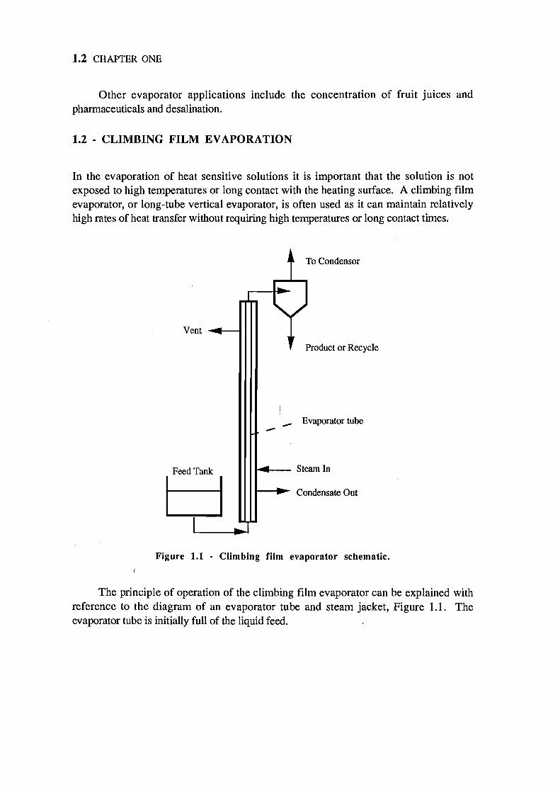
In the evaporation of heat sensitive solutions it is important that the solution is· not exposed to high temperatures or long contact with the heating surface. A climbing film evaporator, or long-tube vertical evaporator, is often used as it can maintain relatively high rates of heat transfer without requiring high temperatures or long contact times.
j Il To Condensor
~) Vent .... -... --t
Product or Recycle
_ Evaporator tube -Feed Tank ~ ... -- Steam In
y~ Condensate Out
Figure 1.1 - Climbing film evaporator schematic.
The principle of operation of the climbing film evaporator can be explained with reference to the diagram of an evaporator tube and steam jacket, Figure 1.1. The evaporator tube is initially full of the liquid feed.
INTRODUCTION 1.3
As steam is supplied to the steam jacket, the liquid in the tube boils and expanding bubbles begin rising rapidly in the tube. Vapour drags a high velocity liquid film up the tube. Lower down the tube the vapour appears in expanding bubbles and higher up the tube a core of high velocity vapour with an annulus of boiling liquid exists. The ratio of length to diameter of the evaporator tube is important for a true 'climbing film' effect. A figure between 100:1 and 160:1 is recommended by QVF, the manufacturer of the pilot plant evaporator used in this work. The result of the climbing film effect is to maintain a thin turbulent film of liquid in contact with the heating surface for a very short time, due to the high velocity of the liquid film.
Climbing film evaporators are usually operated under vacuum. The vacuum reduces the boiling temperature of the feed solution and improves the temperature difference for heat transfer from the steamjacket.
Previous studies of climbing film evaporation have been made by Coulson and Mehta (1953), Coulson and McNelly (1956), Gupta and Holland (1966), Tang (1980) and Bourgouis and Le Maguer (1983, 1984, 1987) who all looked at steady-state heat transfer only.
1.3 . TWO·PHASE FLOW
The topic of two-phase flow is important in the mathematical description of the behaviour of the climbing film evaporator. A variety of two-phase flow models can be derived following a few basic principles. A general text on transient models of two-phase flow is Ishii (1975). Stewart and Wendroff (1984) present an equal pressure model, which consists of a set of six partial differential equations; the equations of continuity, momentum and energy transport for each phase. The model describes the non-steady state flow of the two phases.
The model can be simplified immediately by the one-dimensional flow assumption that presumes there is no radial variation across the evaporator tube, so physical quantities are in effect radial averages.
A number of other simpler models may be derived from the model. If friction is large, the two phases will move with almost equal velocities. If this situation is approximated by supposing that the velocities are identically equal, and appropriate average properties are defined, the so-called homogeneous flow equations result. This assumption of homogeneous flow yields the simplest model of two-phase flow - a set of three partial differential equations of homogeneous continuity, momentum and energy transport. In effect, the two-phase mixture is considered a pseudo-fluid that obeys the single-phase gas dynamics equations without concern for a detailed description of the flow pattern.
1.4 CHAPTER ONE
Wallis (1969) includes a chapter on homogeneous flow. Kaka9 and Veziroglu (1982) used one-dimensional homogeneous models to model two-phase flow dynamics. Stewart and Wendroff (1982) include in their discussions a homogeneous model which they tenn an equal velocity model.
1.4 . MODELLING AND IDENTIFICATION
System identification is the experimental approach to model building. The topic of system identification includes the construction, estimation of parameters and validation of mathematical models of dynamic systems based upon observed data.
The climbing film evaporator is a distributed parameter system, characterised by the fact that the system states depend on spatial position as well as time. For a onedimensional model the spatial variable is the distance along the length of the evaporator tube. The system is described by partial differential equations relating the system states in space and time. A lumped parameter system differs from a distributed parameter system as the fonner is described by ordinary differential equations and there is no spatial dependence.
The relationship between a lumped parameter system and a distributed parameter system is illustrated by the following example.
A common first-order model for an industrial process, with state u(x,t), time delay Td, gain Kp and time constant 1: is given by the following transfer function between u(xt.t) and U(X2,t)
G(s) = Kp e-sTd
1:S + 1
where t is time, x denotes distance and s is the Laplace variable.
This process can be partly described by the following hyperbolic distributed parameter system
aU(X,t) + iJu(x,t) + b ( t) - 0 at a ax u,X,-
where a and b are constants.
IN1RODUCTION 1.S
The relationship between the two equations is
T Xl - X2 d= a
where Xl and X2 denote two separate spatial positions.
The time constant 'r does not appear in the partial differential equation but can be incorporated by augmenting the distributed parameter system with a first-order linear differential equation. The time constant simulates the effect of diffusion, which distorts the shape of an input pulse propagating through the distributed parameter system.
There are two major approaches in the modelling and identification of distributed parameter systems. The first approach consists of initially lumping the parameters of the distributed parameter system model and applying the identification and control methods for lumped parameter systems to the resulting ordinary differential equations. This is usually the first step in the identification of distributed parameter systems. The simplest type of model description is a linear model where the parameters of the model are timeinvariant. These models are often linearisations of non-linear systems and they idealise the real process, but they give good results in many situations.
There is a plethora of texts on lumped parameter system identification and numerous surveys in the literature of identification methods for linear time invariant systems, Isermann et al (1973), Ljung and Soderstrom (1983), Ljung (1987) and, Soderstrom and Stoica (1989). A linear time-invariant lumped parameter model of an industrial evaporator that has been identified using these techniques is presented by Crawford and Austin (1988).
The alternative approach is to apply the modelling and identification theory for distributed parameter systems to identify the distributed states of the system. Polis and Goodson (1976), Kubrusly (1977) and Polis (1982) survey the methods used in distributed parameter system identification and Ray (1978) presents a survey of applications of distributed parameter system theory. In particular, Carpenter et al (1971) detail the solution of distributed parameter systems described by hyperbolic partial differential equations using the method of characteristics.
1.6 CHAPTER ONE
SYMBOLS
a A constant
b A constant
G(s) Laplace transfer function
Kp Gain
s Laplace variable
Time
Td Time delay
't' Time constant
u(,x,t) State variable
x Distance
Subscripts
1 Spatial position 1
2 Spatial position 2
REFERENCES
Bonrgois, J. and Le Magner, M.,"Modeling of Heat Transfer in a Climbing Film
Evaporator: Part /", J. Food Eng., Vol. 2, pp63-75 (1983).
Bonrgois, J. and Le Magner, M., "Modeling of Heat Transfer in a Climbing Film
Evaporator: Part Ir, J. Food Eng., Vol. 2, pp225-237 (1983).
Bonrgois, J. and Le Magner, M.,"Modeling of Heat Transfer in a Climbing Film
Evaporator: III. Application to an Industrial Evaporator", J. Food Eng,. Vol. 3, pp39-50 (1984).
Bonrgois, J. and Le Magner, M., "Heat Transfer Correlation for Upward Liquid Film Heat
Transfer with Phase Change: Application in the Optimization and Design of Evaporators", J. Food Eng., Vol. 6, pp 291-300 (1987).
INTRODUCTION 1.7
Carpenter, W.T., Wozny, M.J. and Goodson, R.E., "Distributed Parameter
Identification Using the Method of Characteristics", Trans. ASME, J. Dynamic Systems,
Measurement and Control, Vol. 93, pp73-78 (1971).
Coulson, J.M. and Mehta, R.R., "Heat Transfer Coefficients in a Climbing Film
Evaporator", Trans. Instn Chern. Eng., Vol. 31, pp208-228 (1953).
Coulson, J.M. and McNelly, M.J., "Heat Transfer Coefficients in a Climbing Film
Evaporator. Part II", Trans. Instn Chern. Eng., Vol. 34, pp247-257 (1956).
Crawford, R.A. and Austin, P.C., "Control of an Evaporator", Proc. 3rd Int. Symp. on
Process Systems Engineering, Sydney, Australia, pp200-205 (1988).
Edgar, T.F., "Automatic Control Opportunities in Industrial Energy Utilization", Proc of the
Int Autom Control Conf, An ASME Century 2 Emerging Technol Conf, vI, San Franciso,
California, Publ on behalf of Am Autom Control Council, Pap n WP7-C, (1980).
Gupta, A.S. and Holland, F.A., "Heat Transfer Studies in a Climbing Film Evaporator.
Part I. Heat Transfer from Condensing Steam to Boiling Water", Can. J. Chern. Eng., pp77-81
(1966).
Gupta, A.S. and Holland, F.A., "Heat Transfer Studies in a Climbing Film Evaporator.
Part II. Heat Transfer Regions", Can. J. Chern. Eng., pp326-329 (1966).
Isermann, R., "Comparison and Evaluation of 6 On-line Identification and Parameter
Estimation Methods with 3 Simulated Processes", Proc. Symp. on Identification and Parameter
Estimation, The Hague/Delft, The Netherlands, Pergamon Press, (1973).
Ishii, M., "Thermo-Fluid Dynamic Theory of Two-phase Flow", Eyrolles (1975).
Kaka~, S. and Veziroglu, T.N., "A Review of Two-phase Flow Instabilities", Advances in
Two-phase Flow and Heat Transfer Vol II, Eds. Kaka~,S. and Ishii,M., NATO ASI Series,
Spitzingsee, Germany, (1982).
Kubrusly, C.S., "Distributed parameter system identification. A survey", Int. J. Control,
Vo1.26, No.4, pp509-535 (1977).
Ljung, L., "System Identification - Theory for the User", Prentice-Hall (1987).
1.8 CHAPTER ONE
Ljung, L. and Soderstrom, T., "Theory and Practice of Recursive Identification", MIT Press
(1983).
Polis, M.P., "The Distributed System Parameter Identification Problem: A Survey of Recent
Results", Proc. 3rd IFAC Symp. on Control of Distributed Parameter Systems, Tolouse, France,
pp45-58 (1982).
Polis, M.P. and Goodson, R.E., "Parameter Identification in Distributed Parameter
Systems: A Sythesizing Overview", Proc. lEEE, Vol. 64, No.1, pp45-61 (1976).
Ray, W.H., "Some Recent Applications of Distributed Parameter Systems Theory - A Survey",
Automatica, Vo1.14, pp281-287 (1978).
SOderstrom, T. and Stoica, P., "System Identification", Prentice-Hall (1989).
Stewart, H.B. and Wendroff, B., "Two-Phase Flow: Models and Methods", Journal of
Computational Physics, Vol 56, pp363-409 (1984).
Tang, C.L., "Two Phase Flow in a Climbing Film Evaporator", Can. J. Chern. Eng., Vol. 58,
pp425-430 (1980).
Wallis, G.B., "One-dimensional Two-phase Flow", McGraw-Hill (1969),
CHAPTER
TWO
EXPERIMENTAL APPARATUS
In which the specifications and operating procedure for the climbing film evaporator are described. The data collection unit and methods of process variable measurement are detailed along with a brief description of the operating program for the climbing film evaporator.
2.1 - CLIMBING FILM EVAPORATOR
2.1.1 - Description
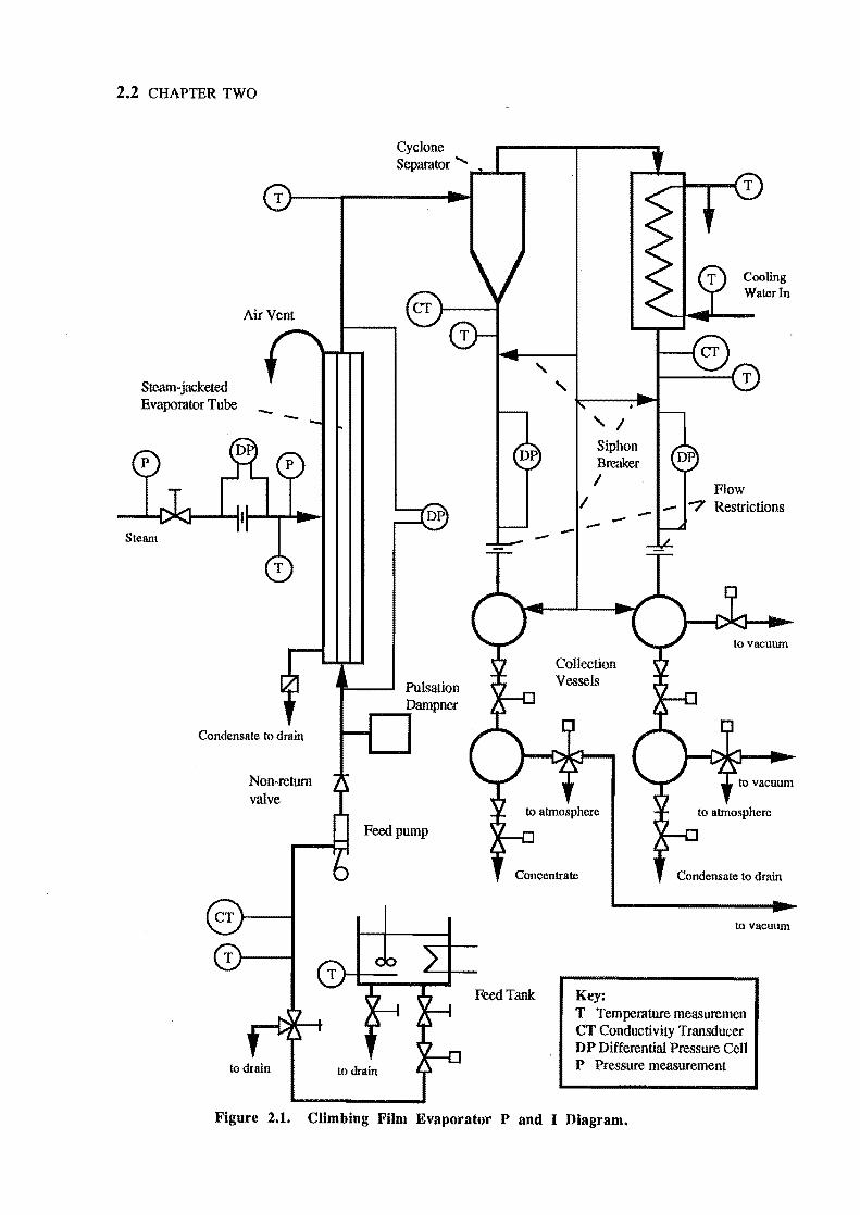
The climbing film evaporator used in this research was a QVF pilot-plant climbing film evaporator. It consisted of a single 3 m long, 1 in diameter steam jacketed evaporator tube with a normal steam consumption of 20 kg/hr. Figure 2.1 is a Piping and Instrumentation Diagram of the climbing film evaporator.
The unit was designed for the evaporation of heat sensitive materials where it is necessary to avoid exposure of the material to high temperatures or a long contact time with the heating surface. The solution concentrated by the evaporator in this study was an aqueous sodium nitrate solution.
The vapour and liquid from the evaporator tube were separated in a centrifugal cyclone separator. The concentrate was collected in a receiving vessel for removal and the vapour passed to the condensor before collection and removal. The unit normally operated under vacuum so that the concentrate and condensate removal was effected by a solenoid sequencer controlling the solenoid valves around the collection vessels. A vacuum supply of 10 inHg was provided by a Nash AL671 vacuum pump.
2.1
2.2 CHAPTER TWO
Cyclone Separator ...... ..,a. ..... --.
Tl----r-----., ......
Air Vent
Steam-jacketed Evapomtor Tube
Condensate to drain
Non-return valve
Pulsation __ .. Dampner
Feed pump
,
-
, ,
/ Siphon Breaker /
/ ---
Collection Vessels
Cooling Water In
Flow Restrictions
to vacuum
Concentrate Condensate to drain
Feed Tank
to drain
to vacuum
Key: T Tempemture measure men CT Conductivity Transducer D P Differential Pressure Cell P Pressure measurement
Figure 2.1. Climbing Film Evaporator P and I Diagram.
EXPERIMENTAL APPARATUS 2.3
2.1.1.1 - Feed Tanks
The evaporator was fed from two heated and stirred feed tanks which were capable of holding 280 litres of feed solution each. The tanks were constructed in mild steel and corrosion protected as follows. After abrasive blast cleaning the steel surfaces two coats of Epiguard 116 Epoxy Primer were applied, followed by a third coat of Epiguard 199 Surfacer and two further coats of Epithane 343 Polyurethane.
Each tank had a 5 kW heater which was controlled by a Temperature Controller unit built by the Chemical and Process Engineering Department, Appendix III. A thermistor bridge was used to sense the temperature and switch 230 V power to the heating elements. A temperature setpoint of the feed solution in each feed tank was maintained within 5°C. The setpoint was adjustable by front panel knobs. A digital circuit provided stable power control to the elements so that the minimum amount of power could be fed to the controlled elements. The exit pipe extended up from the bottom of the tank so that the heater elements were always submerged in the feed solution.
In addition to manual valves on the output from the tanks, solenoid valves were installed so that the tank outlets could be opened and closed automatically via two solid state relays which were controlled by computer. The switching circuit is in A ppendix III.
The feed solution was also continuously stirred by a stirrer motor and impeller installed for each tank.
2.1.1.2 - Feed Pump
The evaporator was fed by a "Jesco" Model MD40 dosing pump manufactured by "Jesco" Dosing Controls, Germany. The pump head was manufactured in polypropylene with a teflon diaphragm to handle a 10 % salt solution at 60°C. The pump injection rate was controlled by an inbuilt sensor receiving a 4-20 rnA signal to vary the pump rate over a range of 4-80 strokes/min. A feed pump module accepted a 0-10 V local or remote setpoint and converted it to a 4-20 rnA value for this sensor. The circuit is found in Appendix III.
As the feed was delivered into a vacuum, a tlJesco" loading valve was included in the line to allow back pressure for the pump and prevent air pockets forming.
2.4 CHAPTER TWO
The positive displacement pump produced a pulsating flow. The pulsations clearly upset the flow pattern of the climbing film and shocked the tube itself, so it was necessary to damp these pulsations. A surge chamber or air vessel was designed and installed to rectify this problem. Details on the design are found in Appendix IV.
2.1.1.3 - Steam Flow Control
The steam flow supply was generated at 80 psig, with a saturation temperature of 163°C and was reduced to 30 psig with a saturation temperature of 135°C by a Birkett 470 pressure reducing valve.
The steam flow to the evaporator steam jacket was then controlled by a PI controller designed and constructed by the Chemical and Process Engineering Department, Appendix III. An auto/manual switch was included to allow manual adjustment of the steam flow. The controller accepted 0-10 V signals for the steam flow value and the desired setpoint. The setpoint could be set locally by a knob on the front panel of the controller or remotely from the operating program. The output of the controller was a 1-5 rnA signal which was converted to a 3-15 psi signal (circuit in Appendix III) and sent to a 1/2 in Honeywell V5011 pneumatic valve and actuator.
2.1.1.4 - Vacuum Pressure Control
The vacuum pressure was controlled by a locally designed and built module which accepted 0-10 V signals proportional to the vacuum pressure and to the desired vacuum setpoint and sent signals to solid state relays which open and shut two solenoid valves -one connected to the buffer tank vacuum, the other to atmosphere. Appendix III has the circuit diagram for this unit. The setpoint could be set manually from a knob on the front panel or received remotely from the control program. It was also possible to manually override the automatic settings and open or shut the two solenoid valves.
2.1.1.5 - Solenoid Sequencer
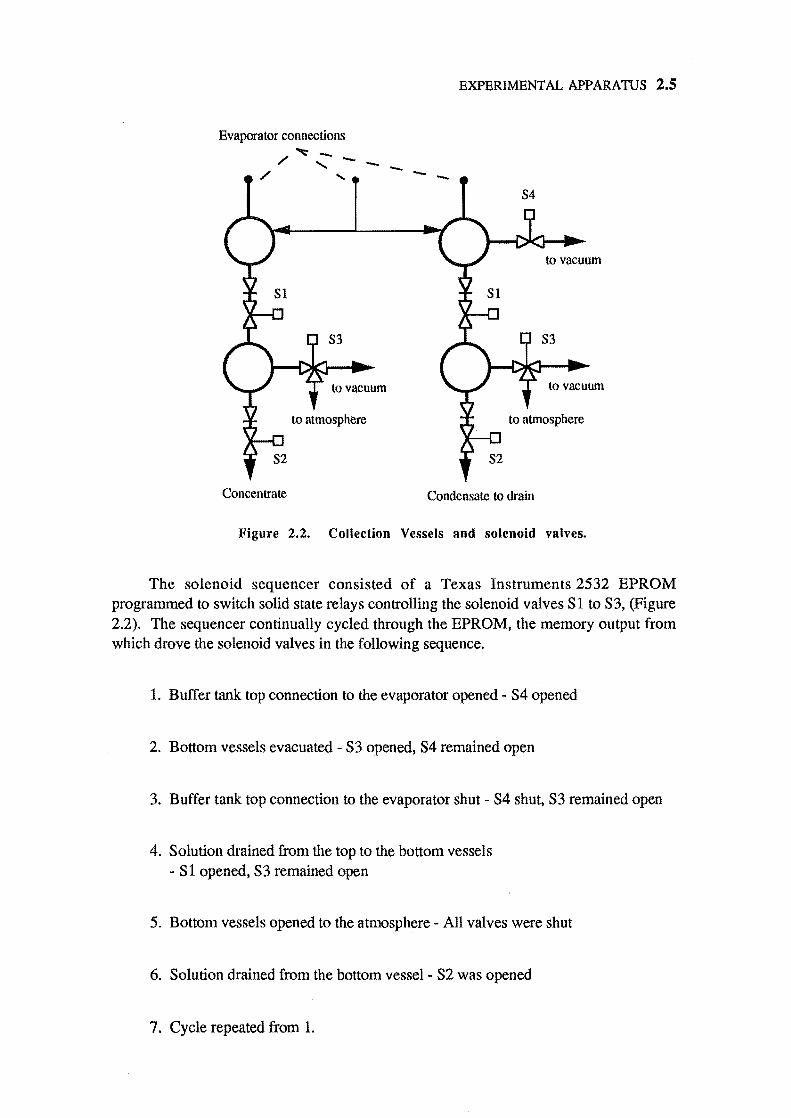
Because the evaporator unit operated under vacuum the concentrate and condensate removal was effected by a solenoid sequencer controlling the sequence of opening and shutting the ~olenoid valves around the collection vessels.
Evaporator connections
/
/"";;' -...... - -.....
S3
to vacuum
EXPERIMENT AL APPARATUS 2.S
Concenlrate Condensate to drain
Figure 2.2. Collection Vessels and solenoid valves.
The solenoid sequencer consisted of a Texas Instruments 2532 EPROM programmed to switch solid state relays controlling the solenoid valves Sl to S3, (Figure 2.2), The sequencer continually cycled through the EPROM, the memory output from which drove the solenoid valves in the following sequence.
1. Buffer tank top connection to the evaporator opened - S4 opened
2. Bottom vessels evacuated - S3 opened, S4 remained open
3. Buffer tank top connection to the evaporator shut - S4 shut, S3 remained open
4. Solution drained from the top to the bottom vessels - Sl opened, S3 remained open
5. Bottom vessels opened to the atmosphere - All valves were shut
6. Solution drained from the bottom vessel - S2 was opened
7, Cycle repeated from 1.
2.6 CHAPTER TWO
2.1.2 - Operating Procedures
The following actions were performed during the startup and shutdown of the evaporator.
Startup:
1. All the sensing equipment - temperatures, pressures and conductivity measurements - and the controller modules were turned on.
2. The heaters and stirrers for the solutions in the feed tanks were switched on.
3. The vacuum pump was turned on.
4. A vacuum was set up in the evaporator - according to the value of the local or remote setpoint.
5. The automatic solenoid sequencer was turned on to allow condensate and concentrate to flow from the evaporator.
6. The outlet valves from the feed tanks were opened.
7 The feed pump was turned on - the desired feedrate detennined by the value of the local or remote setpoint.
8. The cooling water inlet valve to the condensor was opened.
9. The instrument air for the steam valve positioner was turned on by opening the instrument air supply valve.
10. :The manual steam supply valve was opened.
11. The orifice plate tapping valves were opened and the steam differential pressure transmitter turned on. This was carefully perfonned as outlined in the Yokogawa model UNEll differential pressure transmitter manual so as not to damage the internal diaphragm.

EXPERIMENTAL APPARATUS 2.7
12. The automatic steam valve was opened manually and switched from the manual setting to automatic control. The steam setpoint value may have been either a local or a remote value.
Shutdown:
1 . The steam controller was switched to manual and the automatic steam valve closed.
2. The manual steam supply valve was closed.
3. The instrument air supply valve was closed.
4. The feed pump was turned off.
5. The feed tank outlet valves were shut.
6 The heaters and stirrers for the feed tanks were turned off.
7. The condensor cooling water valve was closed.
8. The orifice plate tapping valves were carefully closed according to the operating procedure recommended in the Y okogawa model UNE 11 differential pressure transmitter manual.
9. The evaporator was brought back up to atmospheric pressure by increasing the vacuum pressure setpoint to atmospheric pressure.
10. The automatic solenoid sequencer was switched off.
11. The vacuum pump was turned off.
12. All the sensing and control gear was switched off.
2.8 CHAPTER TWO
2.2 . DATA COLLECTION UNIT
2.2.1 . Description
The data collection unit consisted of a Motorola 6809 microprocessor and assorted peripheral devices. The unit was developed within the Chemical and Process Engineering Department at the University of Canterbury. Information from various sensors was collected by the Analog-to-Digital (A-to-D) converters mounted in the unit. Analog signals were sent to the process via Digital-to-Analog (D-to-A) converters. Peripheral Interface Adapters (PIAs) were also available to allow input and output of onoff signals.
The values sent to and received from the data collection unit were the internal digital representation of an input or output variable and were dependent on the resolution of the A-to-D or D-to-A converter. Thus a 0 to 10 V signal passing through a 12 bit A-to-D converter was converted to a number in the range 0 to 4095.
Commands were sent to the data collection unit through one of two serial ports and consisted of a command character, '-" followed by a request to either read from, or write to, a data register. Each of the data registers was mapped to a peripheral device. For example, the command '-P,O<CR>' would request the value from the first input register and the command '-S,2,255<CR>' would send the value 255 to the third output register.
Characters which were received by the unit through a serial port and not contained between a ,_, and a carriage return were transmitted to the second serial port. The unit could act as a data collection/control device and still maintain transparent communication between the terminal and computer by attaching one serial port to a computer and the other to a terminal. The computer could then interrogate the unit for data whilst maintaining output to the terminal. The unit was placed between the departmental VAX I1n30 minicomputer and the operator terminal.
The evaporator was controlled by an operating program running on the V AX which requested data from the unit and manipulated the process setpoints by using the unit's output registers.
2.2.2 - Connection of Process Sensors and Controls
The following instruments and devices connected to the evaporator, as shown in Figure 2.1, sent signals to and received signals from the data collection unit:
Conductivity cells - 3 A-to-D connections
EXPERIMENTAL APPARATUS 2.9
Temperature sensors - to A-to-D connections
Pressure sensors - 5 A-to-D connections
Feed pump - 1 D-to-A connection
Steam flow PI controller - 1 D-to-A connection
Vacuum pressure controller - 1 D-to-A connection
Tank solenoid valves - 2 D-to-A connections
The temperature and pressure sensors produced signals in milli-volts which were amplified by amplifier modules to 0 toto V signals and digitised by the data collection unit to yield numbers of range 0 to 4095 (12 bits). The 4 to 20 rnA signals produced by the conductivity sensors were also converted to 0 to to V signals before being digitised by the data collection unit.
The feed pump flowrate was controlled through one D-to-A connection. The command '-S,O,O<CR>' output 0 V to the pump controller to request minimum flow and '-S,0,255<CR>' output to V to obtain maximum flow of 0.8 kg/min.
The second D-to-A converter sent a 0 to 10 V setpoint signal corresponding to o to 0.2167 kg/min to the PI controller controlling the steam flow to the steam jacket of the evaporator.
The third D-to-A converter was used to send a 0 to 10 V setpoint value to the vacuum pressure controller on the evaporator. '-S,2,0<CR>' requested an absolute vacuum (not practically attainable) and '-S,2,255<CR>' set the evaporator pressure to atmospheric.
Two D-to-A lines were also used to open and shut the discharge valves from the two feed tanks. These lines controlled the switching of the two solid state relays which controlled the solenoid valves on the exit flow of each of the tanks. The command '-T,O<CR>' shut both tanks, '-T,1<CR>' opened the first tank only, '-T,2<CR>' the second tank only and '-T,3<CR>' opened both tanks.
2.10 CHAPTER TWO
2.3 • PROCESS VARIABLE MEASUREMENT
2.3.1 • Steam Flowrate Measurement
The steam flow to the steam jacket was inferred from the pressure drop across a 7.5 mm orifice plate with D tappings. The pressure drop was measured with a Yokogawa differential pressure transmitter, model UNEll and the 4-20 mA signal converted to a o t010 V signal for use by the operating program and the steam flow controller. Appendix III has the circuit diagram for the current-voltage converter. The steam flow was calibrated by measurement of the condensate using a bucket and stopwatch and a linear regression equation was fitted (Appendix II).
2.3.2 - Vacuum Pressure Measurement
The vacuum pressure was measured by a National LX0503A pressure transducer and the resultant milli-volt signal was amplified to 0 t010 V. The amplifier circuit is found in Appendix Ill. The sensor was calibrated so that 0 to 10 V corresponded to 0 to 1 atm.
2.3.3 - Output Flowrate Measurement
The output flowrates were calculated from measurement of the differential pressure over a flow restriction in a length of 1/2in diameter tube feeding each of the collection vessels. The differential pressures were measured by a Micro Switch 140PC pressure transducer and the resulting milli-volt signal amplified to 0 to 10 V. The sensors were calibrated so that a signal range of 0 t010 V corresponded to 0 to 5 psid. The flows were calibrated using a bucket and a stopwatch and a regression equation fitted. The flowrate equations with regression values are included in Appendix II.
2.3.4 - Concentration Measurement
The solution concentrations were inferred from conductivity and temperature measurements. The conductivities were measured with Philips PW9570/02 fourelectrode flow line cells and PW9521/20 conductivity transmitters. The 4-20 mA outputs of the transmitters were then converted to a 0 to10 V signal using the standard conversion circuit, (Appendix III). These outputs corresponded to conductivity ranges of 0 to ~;oOmS/cm for the feed and concentrate cells and 0 to 1000 mS/cm for the condensate cell. The temperature measurement was as described in section 2.3.5. The conductivity and temperature were measured for solutions of known concentration to provide the calibration data. This data was then fitted using a multi-variable regression equation based on the empirical Vogel-Tammann-Fulcher equation for the conductivity of concentrated solutions. Details are to be found in Appendix II.
EXPERIMENTAL APPARATUS 2.11
2.3.5 - Temperature Measurement
The climbing film evaporator internal temperatures were measured with National LM335H temperature transducers and the signals amplified to a range of o to10 V. The amplifier circuit is in Appendix III. The sensors were soldered using "easy-flo" into stainless steel tubes and the tubes were filled with silicon grease to protect against damage from moisture. The sensors were calibrated so a signal of 0 to 10 V corresponded to 0 to 100·C for the internal evaporator temperatures, and 0 to 150·C for the steam and steam condensate temperature measurements.
2.4 • EVAPORATOR OPERATION SOFTWARE
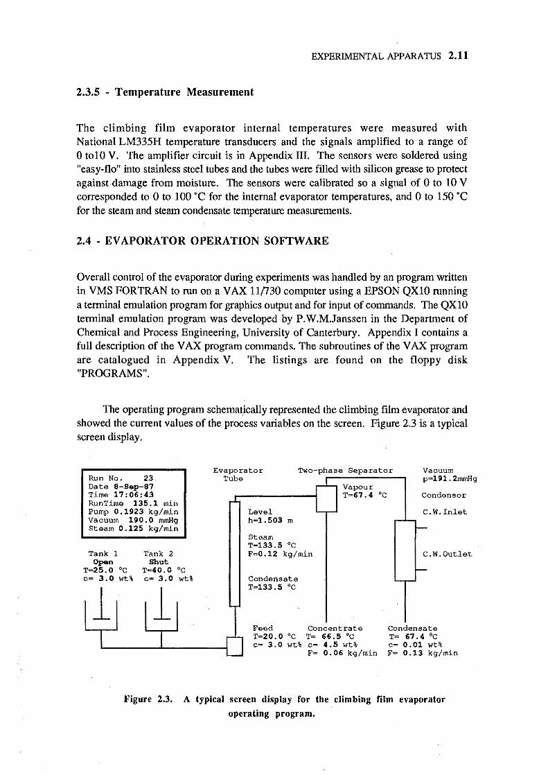
Overall control of the evaporator during experiments was handled by an program written in VMS FORTRAN to run on a VAX 11n30 computer using a EPSON QXlO running a terminal emulation program for graphics output and for input of commands. The QXlO terminal emulation program was developed by P.W.M.Janssen in the Department of Chemical and Process Engineering, University of Canterbury. Appendix I contains a full description of the VAX program commands. The subroutines of the VAX program are catalogued in Appendix V. The listings are found on the floppy disk "PROGRAMS".
The operating program schematically represented the climbing film evaporator and showed the current values of the process variables on the screen. Figure 2.3 is a typical screen display.
RUn No. 23 Date S-Sap-S7 Time 17:06:43 RunTime 135.1 min Pump 0.1923 kg/min Vacuum 190.0 mmHg Steam 0.125 kg/min
Tank 1 Open
T=25.0 °c c= 3.0 wt%
1 Tank 2
Shut T=40.0 °c c= 3.0 wt%
1
EVaporator Two-phase Separator Vacuum p-191.2mmHg Tube
Level h=1.503 m
Steam T=133.5 °c F=0.12 kg/min
Condensate T=133.5 °c
Vapour T=67.4 °c
Feed Concentrate T=20.0 °c T- 66.5 °c c= 3.0 wt% c= 4.5 wt%
F= 0.06 kg/min
Condensor
C.W. Inlet
C.W.Outlet
Condensate T= 67.4 "c c= 0.01 wt% F= 0.13 kg/min
Figure 2.3. A typical screen display for the climbing film evaporator
operating program.
2.12 CHAPTER TWO
Using the program, the operator could open or shut either or both of the feed tanks and alter the feed pump flowrate, the steam flowrate and the vacuum pressure supplied to the evaporator. Upon a shutdown request from the operator, the program performed the automatic tasks of the shutdown procedure.
The data acquisition unit acted as the interface between the V AX and the process making available evaporator measurements to the operating program. By employing the appropriate data acquisition commands, data collection and control of the evaporator was facilitated. The output of screen information remained transparent to the data acquisition unit. Subroutines converted the measured variables to engineering units for display and logging to file by the use of regression calibrations. Operator-entered setpoints were converted to numerical values for output to the evaporator control equipment from the data acquisition unit.
CHAPTER
THREE A DISTRIBUTED PARAMETER
MODEL OF THE EV APORA TOR
For a rigourous description of the climbing film evaporator, the evaporator should be modelled by a set of partial differential equations in space and time. In this chapter such a model is presented.
3.1 • ONE DIMENSIONAL TWO·PHASE HOMOGENEOUS FLOW EQUATIONS
The first assumption of this model is of one-dimensionality. The mathematics are simplified considerably by presuming that there is no radial variation of the system states across the evaporator tube, so that the physical quantities are effectively radial averages.
In the Introduction it was noted that homogeneous flow theory provides the simplest technique for analysis of two-phase flows. In homogeneous flow the mixture is considered a "pseudo-fluid" that obeys the single-phase gas dynamics equations. This assumption is valid for the case where the frictional forces are large. Average fluid properties are then defined accordingly. A detailed description of the flow pattern is not required for this method and thus droplet flow, bubbly flow, or annular flow are all treated exactly the same (Wallis, 1969),
3.1
3.2 CHAPTER THREE
The homogeneous density of the pseudo-fluid is defined as the average of the liquid and vapour density
P = apg + (1 - a) PI
where P = homogeneous mixture density, a = void fraction (volume fraction of the vapour phase), Pg = vapour density, PI = liquid density.
(3.1)
The differential equations of continuity, momentum and energy (Wallis, 1969) for unsteady-state one-dimensional flow are:
Continuity
Momentum (au au) ~ 4 P at + u az = - az -D 't'w
where u = homogeneous mixture velocity, t = time, z = distance up the evaporator tube, p = evaporator pressure, D = evaporator tube diameter, 't'w = evaporator tube wall shear stress, e = internal energy, h = homogeneous mixture enthalpy, A = evaporator tube cross sectional area, q = heat input along the evaporator tube, w = shaft work.
(3.2)
(3.3)
DISTRIBUTED PARAMETER MODEL 3.3
The momentum equation (3.3) may be developed further by expressing the wall shear stress in terms of a friction factor, Cf. The wall shear stress is given by
(3.5)
and
(3.6)
The energy equation (3.4) can be extended by using Wallis' development. Substituting the identity
pe:::: ph - p (3.7)
Expanding the energy equation (3.4), and substituting the continuity (3.2) and momentum (3.6) equations, gives
dh + u dh = 1 (~+ u i!J!.) + U .! 'fw + _1 (~_~) at dz P at dz p D Ap dz (jZ
(3.8)
3.2 • DEVELOPMENT OF AN EVAPORATOR MODEL
During a transient, the pressure changes and viscous dissipation are small compared with the other energy terms. There is no shaft work and the heat flux due to heat transfer from the steam jacket, and including evaporation, is given by
(3.9)
where q, = heat flux, hi = internal heat transfer coefficient from the evaporator steam jacket to the fluid, T w :::: evaporator steam jacket temperature, T:::: homogeneous mixture temperature.
The energy equation (3.8) becomes
(3.10)
3.4 CHAPTER THREE
Now by making use of the relation
r)" dh = CpdT --
P (3.11)
where Cp is heat capacity, ris the evaporation rate per unit volume, and)., is the latent heat of vaporisation, the following development of the energy equation is obtained
(3.12)
To express the evaporation rate r in terms of known variables, the vapour phase continuity equation is considered
(3.13)
Expanding the differentials and substituting the definition of P (equation 3.1) and the homogeneous continuity equation (3.2) yields
r- PIPs au - PI_Pg dz
Th~ energy equation (3.12) then becomes
(3.14)
(3.15)
This set of three equations (3.2, 3.6 and 3.15) has four dependent variables, P, U,
P and T. An equation of state is required to completely specify this problem.
Under the assumption of an ideal gas
p=RpT (3.16)
where R is the universal gas constant, a suitable expression for the differentiallJJi in the
momentum equation is obtained
IlE. _ ~ aT + ~ dp dz - aT dz dp dz
aT dp =Rp-+RT-dz dz (3.17)
DISTRIBU1ED PARAMETER MODEL 3.5
Substituting this relation (3.17) into the momentum equation (3.6) gives
(3.18)
Now this results in a set of three non-linear hyperbolic equations in three dependent variables, p, u, and T, and two unknown model parameters, Cf and hi.
Continuity
Momentum
Energy
dP dP dU ~+u""""'C+p-=O or, OZ dz
dU dU aT dP 0. 2 P at + pu dz + Rp + RT dz = -2 D pu
aT + U aT = 4hi (T w _ T) _ PIPg ~ au at di pCpD Pl-Pg pCp dz
(3.19)
(3.20)
(3.21)
This is complex description of the evaporator behaviour, which is highly nonlinear, requires only two parameters. This may be contrasted with a lumped parameter model whose form is considerably simpler, yet may require many more parameters to provide an accurate simulation. For example, a third order discrete model requires at least six parameters - three parameters are associated with the system's poles, a further three with the system's zeros and possibly one parameter term associated with using actual values of the variables rather than deviations from steady-state.
3.3 - SOLUTION USING THE METHOD OF CHARACTERISTICS
The set of partial differential equations complete with appropriate initial and boundary conditions may be solved using the method of characteristics to yield a complete description of the behaviour of the climbing film evaporator. The method of characteristics, (Smith, 1965), allows the exact solution of a set of hyperbolic partial differential equations, as is the case here, by reducing the problem to the solution of a set of ordinary differential equations.
3.6 CHAPTER THREE
In addition to the constituent equations the following differential relations hold
dp = 1: dt + iJ: dz
aT aT dT=di dt +di dz
For the vector [~f. dUd T d P dud T JT the augmented matrix is: Ul at (ji dz dz dz
1 0 0 u p 0 0
o p 0 RT pu Rp -2fJ pu2
o 0 pCp 0 PIPg it pCpU '1:/ (Tw - n PI-Pg
dt 0 0 dz 0 0 dp
o dt 0 0 dz 0 du
o 0 dt 0 0 dz dT
The equations for the characteristic directions are
(~:)= u, u + R [T + PIPg ;] PI-Pg p
These are labelled the a, f3 and ycharacteristics respectively.
DISTRIBUTED PARAMETER MODEL 3.7
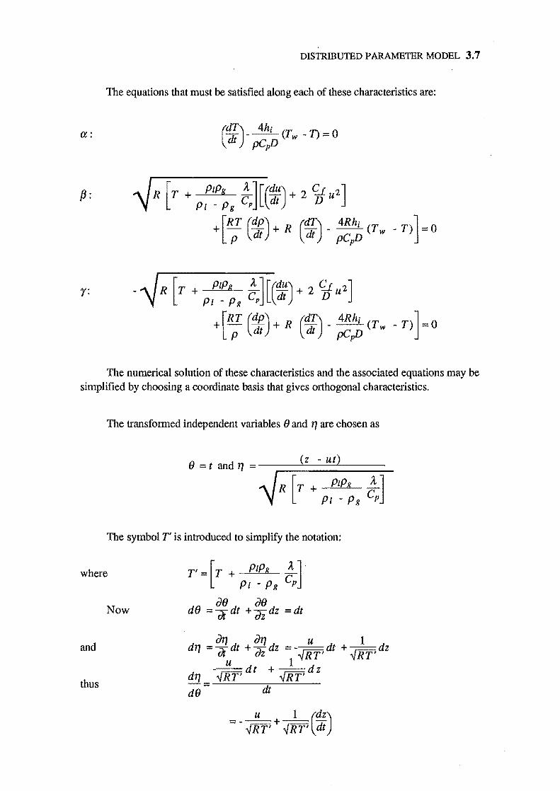
The equations that must be satisfied along each of these characteristics are:
a: (~)- pC,IJ (Tw -n = 0
13: R [T + PIPe !.] [(dU) + 2 CJ. u2] PI - Pg Cp dt D
+ [RT (dP) + R (dT) _ 4Rhi (T _ T)] = 0 P dt dt pC,IJ w
r: R [T + PIPe !.] [(dU) + 2 CJ. u2] PI - Pg Cp dt D
+ [RT (dP) + R (d'[) _ 4Rhj (T w _ T)] == 0 P dt dt) pC,IJ
The numerical solution of these characteristics and the associated equations may be simplified by choosing a coordinate basis that gives orthogonal characteristics.
The transformed independent variables 0 and 1} are chosen as
o == t and 1} == --;::::~( z:=-=u:::t )~:=:=_
R [T + PIPe ~J PI Pg Cp
The symbol T' is introduced to simplify the notation:
where
Now
and an an u 1 d1} =-dt +-dz =---dt + dz de dz ...jRT' ...jRT'
U 1 ---dt + --dz d1} == {lff' {lff' dO dt
thus
3.8 CHAPTER THREE
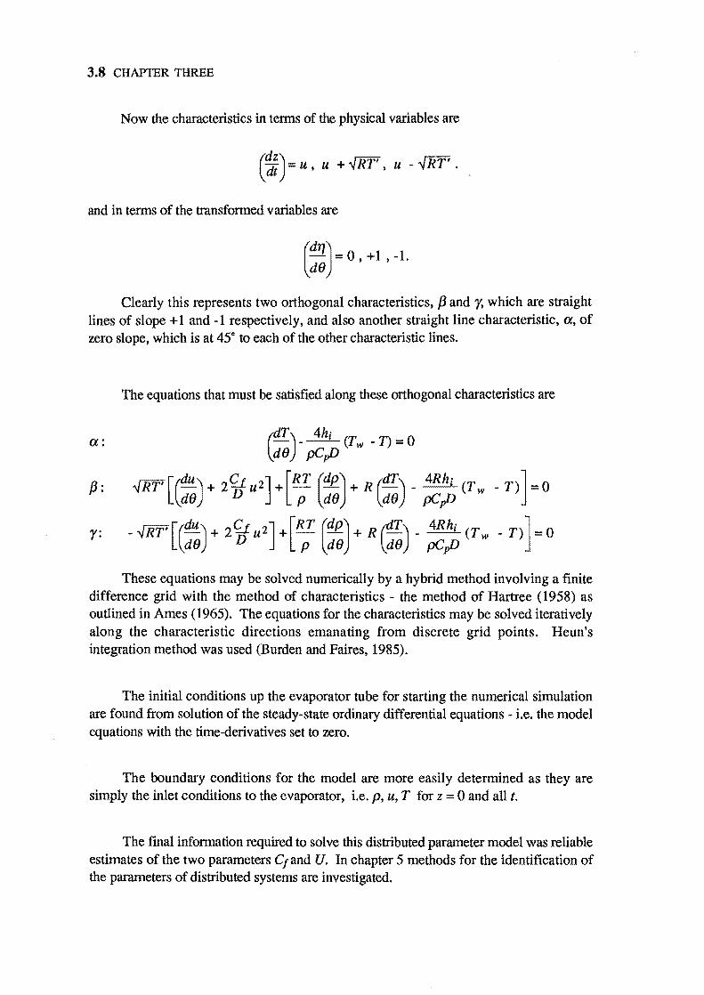
Now the characteristics in tenns of the physical variables are
(~) = U, U + vRT', U - vRT' .
and in tenns of the transformed variables are
(~:)-O.+l.-1.
Clearly this represents two orthogonal characteristics, f3 and r, which are straight lines of slope + 1 and -1 respectively, and also another straight line characteristic, a, of zero slope, which is at 45" to each of the other characteristic lines.
a:
f3:
r:
The equations that must be satisfied along these orthogonal characteristics are
~T) _ 4hi (T - 1) = 0 ld8 pCp£) W
vRT' [(dU) + 20. u2] + [RT (dP) + R (dT) _ 4Rhi (T - T)] = 0 d8 D P d8 d8 pCp£) W
_ vRT' [(dU) + 20. u2] +[RT (dP) + R ~T) _ 4Rhi (T _ T)] = 0 d8 D P d8 ld8 pCp£) W
These equations may be solved numerically by a hybrid method involving a finite difference grid with the method of characteristics - the method of Hartree (1958) as outlined in Ames (1965). The equations for the characteristics may be solved iteratively along the characteristic directions emanating from discrete grid points. Heun's integration method was used (Burden and Faires, 1985).
The initial conditions up the evaporator tube for starting the numerical simulation are found from solution of the steady-state ordinary differential equations - i.e. the model equations with the time-derivatives set to zero.
The boundary conditions for the model are more easily detennined as they are simply the inlet conditions to the evaporator, i.e. p, u, T for z = 0 and all t.
The final information required to solve this distributed parameter model was reliable estimates of the two parameters Cland U. In chapter 5 methods for the identification of the parameters of distributed systems are investigated.

DISTRIBU1ED PARAME1ER MODEL 3.9
SYMBOLS
A Evaporator tube cross sectional area
Cf Homogeneous friction factor
C p Heat capacity
D Evaporator tube diameter
e Internal energy
f A general function
h Homogeneous mixture enthalpy
hi Local internal heat transfer coefficient from the evaporator steam jacket to the fluid
ho Local internal heat transfer coefficient from the steam to the evaporator steam jacket
p Pressure
q Heat input along the evaporator tube
Time
T Homogeneous mixture temperature
T' Transformed mixture temperature for orthogonal characteristics
Ts Evaporator steam temperature
T w Evaporator steam jacket temperature
u Homogeneous mixture velocity
U Overall heat transfer coefficient from the steam to the evaporator fluid
w Shaft work
x Mass fraction of the vapour phase
z Distance up the evaporator tube
a Void fraction M the volume fraction of the vapour phase
3.10 CHAPTER THREE
r Evaporation rate per unit volume
11 Distance variable for orthogonal characteristics
A, Latent heat of vaporisation of steam
¢J Heat flux
8 Time variable for orthogonal characteristics
p Homogeneous mixture density
'fw Wall shear stress
Subscripts
g Vapour phase
Liquid phase
s Steam
w Wall
REFERENCES
Ames, W.F., "Nonlinear Partial Differential Equations in Engineering", Academic Press,
London & New York, pp445-448 (1965).
Burden, R.L. and Faires, J.D., "Numerical Analysis", 3rd Ed., PWS Publishers, Boston,
pp223-224 (1985).
Hartree, D.R., "Numerical Analysis", 2nd Ed., Oxford University Press, London &
New York, (1958).
Smith, G.D., "Numerical Solution of Partial Differential Equations", Oxford University Press,
pp98-130 (1965).
Wallis, G.B., "One-dimensional Two-phase Flow", McGraw-Hill, p35 (1969).
CHAPTER
FOUR
LUMPED PARAMETER IDENTIFICA TION
In which the topic of lumped parameter identification is surveyed for the purpose of application to the climbing film evaporator.
4.1 - INTRODUCTION
As detailed in Chapter 1, the techniques of system identification deal with the problem of constructing mathematical models of dynamic systems based upon observed data from the systems. The climbing film evaporator, along with many other industrial processes, is a distributed parameter system, characterised by the fact that the system states, inputs and outputs may depend on spatial position as well as time. In this case, the spatial variable is the length of the evaporator tube.
The two general approaches taken in the modelling, identification and control of distributed parameter systems are the lumped parameter approach and the distributed parameter approach.
The lumped parameter methods begin by "lumping the parameters" of the distributed parameter system model whereby spatially varying parameters in the evaporator are lumped into one location. Identification methods for lumped parameter systems are then applied to the resulting ordinary differential equations. This first step in the identification of distributed parameter systems is described in this chapter.
4.1
4.2 CHAPTER FOUR
4.2 • LUMPED PARAMETER SYSTEMS
The parameters of the distributed parameter system model have been assumed to be lumped at this stage, so that a lumped parameter model is used as a description of the process. The lumped parameter model is described in section 4.2.1.
Three of the methods for lumped parameter identification were compared. The methods evaluated were recursive least squares (RLS), recursive extended least squares (RELS) and recursive maximum likelihood (RML). These recursive methods were built about a un factorisation algorithm for numerical stability (Biermann, 1977). The methods exhibited biased results in the presence of large noise signals contaminating the output, i.e. they converged to incorrect values of the system parameters. The decision was made to look at the bias in terms of continuous gain and time constants as well as the discrete parameters, as these parameters were adjudged more meaningful to most chemical engineers and it was found to be mathematically simple to convert the identified discrete model parameters to the continuous-time domain.
Known "test" processes in the continuous-time domain were transformed to find the discrete-time equivalent in the z-plane to perform the comparison of the identification methods. An input signal of a pseudo random binary sequence (PRBS) was used to test the identification methods on the discrete model. The output was contaminated with Gaussian white noise of varying standard deviations.
4.2.1 • Mathematical Models
The process to be identified has been assumed to be a continuous process with sampled input signal, u(k), and noise corrupted output, y(k), described by the linear difference equation
y(k) + aly(k-1) + ... + anY(k-n) = b1u(k-d-1) + ... + bnu(k-d-n) + v(k)
where n = model order, d = deadtime in sampling intervals, v(k) = equation error.
(4.1)
The linear difference equation can be written in terms 'of q-l, the delay or backward shift operator (Ljung, 1987), as
A(q-l ).y(k) = B(q-l ).u(k-d) + v(k) (4.2)
LUMPED PARAMETER IDENTIFICATION 4.3
where A = [al ... t1n], the output parameter vector, B = [bl ... bn], the input parameter vector, q-l = y(k-1)/y(k), the backward shift operator.
This model has equation error model structure. The model, equation (4.1) or (4.2) is also called an ARX model (Ljung 1987), where AR refers to the autoregressive part , A(q-l).y(k), and X refers to the exogeneous variable, B(q-l).u(k-d).
If equation (4.2) is rewritten in vector form
y(k) = 9 T(k)qJ(k) + v(k) (4.3)
a linear regression results. 9 is the vector of the parameters which it is desired to establish so that the model of the system, equations (4.1) and (4.2), matches the observed data in section 4.2.3
(4.4)
qJ(k) is known as the regression vector - the observations of the system at time k
cp(k) = [y(k-1) ... y(k-n), u(k-1) ... u(k-n)] (4.5)
The disadvantage of the simple model (4.1) is that the properties of the disturbance are unknown. If the equation error is described as a moving average of white noise the model becomes
y(k) + aly(k-l) + ... + anY(k-n) = blU(k-d-l) + ... + bnu(k-d-n) + e(k) + cle(k-l) + ... + cne(k-n) (4.6)
where C, [et ... cnJ, is the noise model parameter vector.
The model may be rewritten
A(q-l).y(k) = B(q-l).u(k) + C(q-l).e(k) (4.7)
Due to the moving average (MA) part C(q-l )e(k), the model described in equations (4.6) and (4.7) is called ARMAX (Ljung ,1987).
4.4 CHAPTER FOUR
Now the parameter vector, e, is expanded to include the Ci terms that describe the noisemode1
(4.8)
The parameter vector given by (4.8) is then used in the regression equation (4.3) with the regression vector extended by the white noise terms e(k-1) ... e(k-n)
qJ(k) = [y(k-1) ... y(k-n), u(k-1) ... u(k-n), e(k-1) ... e(k-n)] (4.9)
4.2.2 - Recursive Identification Methods
Before discussion of the identification methods it is important to consider why recursive algorithms were used. Recursive methods entail the update of the parameter estimates with each new measurement and are used in on-line applications. The methods only require a small amount of computation at each step, and previous values of the regression and parameter vectors need not be stored. They may also be modified to track timevarying parameters.
The algorithms have been derived by minimising a chosen performance index that measures the discrepancy between the identified model and the actual process. Ljung and SOderstrom (1983) show that the algorithms differ only in the choice of the performance criterion and in the form of the noise model assumed.
Routines implementing the recursive identification algorithms have been written in V AX-FORTRAN and run on a VAX 11n30 minicomputer in the Chemical and Process Engineering department. The program UDUMISO.FOR is the main source file. The listing may be found on the disk labelled PROORAMS with the other source files. These files are catalogued in Appendix V.
4.2.2.1 - Recursive Least Squares (RLS)
Since the least squares method is well known, only the way it has been implemented will be presented. Hsia (1977) presents a complete derivation. RLS uses the ARX model to characterise the process to be identified.
LUMPED PARAMETER IDENTIFICATION 4.5
The recursive algorithm for the RLS method is: .
8(k) = 8(k-1) + L(k) [y(k) - q>T(k)8(k-1)]
L k _ P(k-1)q>(k) ( ) - A(k) + q>T(k)P(k-1)q>(k)
P(k) = P(k-1) _ P(k-1)q>(k)q>T(k)P(k-1) A(k) + q>T(k)P(k-1)q>(k)
= [I - L(k)q>T(k)P(k-1)]P(k-1)
(4.10)
(4.11)
(4.12)
(4.13)
where L(k) is the gain vector, P(k) is the error covariance matrix and A(k) is the forgetting factor.
For numerical stability the algorithm is not implemented in quite this form. The recursive method is instead implemented using a UD factorisation algorithm, (Biermann, 1977). It has been shown by Biermann that the unmodified recursive algorithm will be unstable if the error covariance matrix P fails to remain positive definite. The UD factorisation algorithm overcomes this by updating a factor of the error covariance matrix P such that P is guarantied to stay positive definite, rather than updating P explicitly.
4.2.2.2 - Recursive Extended Least Squares (RELS)
The RELS method (Isermann, 1981) applies to ARMAX model equation (4.6), This enabled properties of the disturbance to be identified. The approach is to cast the ARMAX model in the form of a linear regression (4.3) and to apply the RLS algorithm (4.10)-(4.13) to the model. It is not a true linear regression as values e(k-1) ... e(k-n) of the regression vector are unknown. The RELS principle calculates the error estimate, e(k), by means of the past estimates of the parameters
e(k) = y(k) - 8(k-1).q>T(k) (4.14)
Then the error estimates are used to approximate the white noise sequence, e(k). From this the noise model parameters are estimated. A simple improvement on this algorithm is to use the most recent set of parameter estimates, i.e. 8(k). This was the version of the algorithm that was used in this work.
To guarantee that the true 8 is a possible convergence point, the following modification of the RELS can be used.
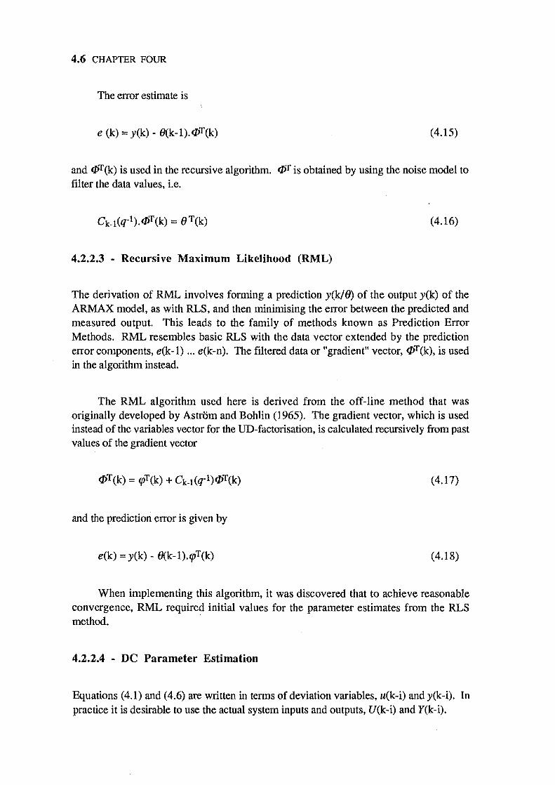
4.6 CHAPTER FOUR
The error estimate is
e (k) = y(k) - 8(k-1). cpT(k) (4.15)
and CPT(k) is used in the recursive algorithm. cpT is obtained by using the noise model to filter the data values, i.e.
(4.16)
4.2.2.3 - Recursive Maximum Likelihood (RML)
The derivation of RML involves forming a prediction y(kl8) of the output y(k) of the ARMAX model, as with RLS, and then minimising the error between the predicted and measured output. This leads to the family of methods known as Prediction Error Methods. RML resembles basic RLS with the data vector extended by the prediction error components, e(k-l) ... e(k-n). The filtered data or "gradient" vector, CPT(k), is used in the algorithm instead.
The RML algorithm used here is derived from the off-line method that was originally developed by Astrom and Bohlin (1965). The gradient vector, which is used instead of the variables vector for the UD-factorisation, is calculated recursively from past values of the gradient vector
(4.17)
and the prediction error is given by
e(k) = y(k) - 8(k-l).q>T(k) (4.18)
When implementing this algorithm, it was discovered that to achieve reasonable convergence, RML required initial values for the parameter estimates from the RLS method.
4.2.2.4 - DC Parameter Estimation
Equations (4.1) and (4.6) are written in terms of deviation variables, u(k-i) and y(k-i). In practice it is desirable to use the actual system inputs and outputs, U(k-i) and Y(k-i).
LUMPED PARAMETER IDENTIFICATION 4.7
The two sets of variables ar~ related by the equations
U(k-i) = Us + u(k-i) and Y(k-i) = Ys + y(k-i) (4.19)
The algorithms presented here may be converted to measured signals by substituting equation (4.19) into the model difference equations (4.1) and (4.6). The result is the addition of a DC term to the parameter vector e, and the use of measured signals in the regression vector 4>.
The estimated DC parameter is given by
n n DC = -Us ~ hi + Ys (1 + ~ ai) (4.20)
i=l i=l
and the corresponding additional entry in the regression vector equals 1.
4.2.2.5 - Values for the Forgetting Factor
For the case of constant parameters, the data at the start of identification may be imperfect due to poor initial estimates. The choice of the forgetting factor A., is important, (Goodwin and Sin, 1984). It is therefore desirable to forget data in this initial phase and let A., increase to 1 with time, i.e. as the effect of the choice of initial conditions decreases. A common way to do this is have
A.,(k) = 8.A.,(k-l) + (1 - 8)
where 8 = 0.98, A.,(O) = 0.95.
(4.21)
This approach is unsuitable for systems where the parameters vary with time. In this thesis the forgetting factor A.,(k) has to chosen so as to maximise the tracking effectiveness of the parameter estimation, while minimising the noise sensitivity of the parameter estimates. Typically a constant value of 0.98 is used for A., in this case.
4.8 CHAPTER FOUR
4.2.3 - Comparison of the Methods
The three methods of recursive identification, described in section 4.2 have been applied to sets of data simulated from two test systems. For these simulated systems the input signal (u(k)} was chosen to be a pseudo random binary sequence of character N(O, 1), (zero mean with unity standard deviation), with a minimum period equal to the sampling period. The sampling period was chosen to have a value of unity.
The two test systems were a first-order plus deadtime transfer function, and a second-order plus deadtirne transfer function, in the continuous-time domain. They were transformed to find the discrete-equivalents in the z-plane by determining the zero-order hold equivalences.
The first-order plus deadtime transfer function was
1.0e-2.Os G(s) = (20s + 1)
where s is the Laplace variable.
The zero-order hold equivalence was then given by
H( -1) = O.04877z-(1+d) z 1 _ O.95123z. 1
where d, the deadtime, had a value of two sampling intervals.
(4.22)
(4.23)
LUMPED PARAME1ER IDENTIFICATION 4.9
Figures 4.1 and 4.2 show the input and output data respectively.
0.1 t-- r-
Q ';i
J 0.0
I -0.1
-0.2 I
0
I I
10 20
Time, t
Figure 4.1. First 50 values of the
1.2
0.9
0.6
0.3 Q ~ ...r 0.0 = §' 0
-0.3
-0.6
-0.9
-1.2
0 300 600
Time. t
Figure 4.2. Output of the First-order plus
-
-
I I I
30 40 50
input signal U (I).
900 1200
dead time system, (Ie :: 0.05.
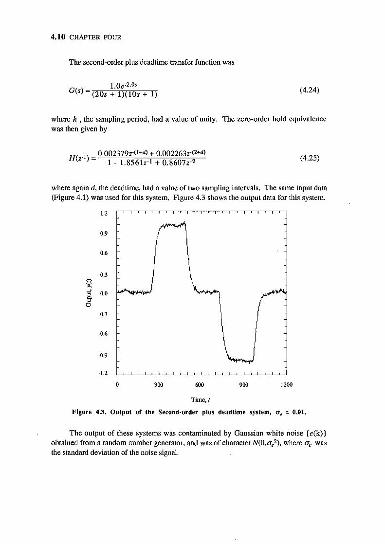
4.10 CHAPTER FOUR
The second-order plus deadtime transfer function was
1.0e-2.Os
G(s) = (20s + 1)(10s + 1) (4.24)
where h , the sampling period, had a value of unity. The zero-order hold equivalence was then given by
-1 _ O.002379z-(1+d) + O.002263z-(2+d) H(z ) - 1 _ 1.8561z-1 + O.8607z-2 (4.25)
where again d, the deadtime, had a value of two sampling intervals. The same input data (Figure 4.1) was used for this system. Figure 4.3 shows the output data for this system.
1.2
0.9
0.6
0.3 Q ~ =r 0.0 g-O
-0.3
-0.6
-0.9
-1.2
0 300 600 900 1200
Time, t
Figure 4.3. Output of the Second-order plus dead time system, (J. = 0.01.
The output of these systems was contaminated by Gaussian white noise (e(k)) obtained from a random number generator, and was of character N(O,(je2), where (je was the standard deviation of the noise signal.
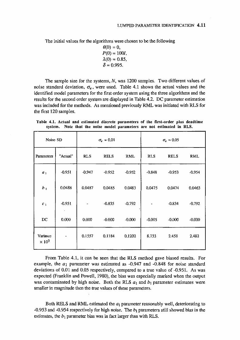
LUMPED PARAMETER IDENTIFICATION 4.11
The initial values for the algorithms were chosen to be the following 0(0) = 0, P(O) = 100/, A(O) = 0.85, 0=0.995.
The sample size for the systems, N, was 1200 samples. Two different values of noise standard deviation, (Ie, were used. Table 4.1 shows the actual values and the identified model parameters for the first order system using the three algorithms and the results for the second order system are displayed in Table 4.2. DC parameter estimation was included for the methods. As mentioned previously RML was initiated with RLS for the first 120 samples.
Table 4.1. Actual and estimated discrete parameters of the first-order plus deadtime system. Note that the noise model parameters are not estimated in RLS.
Noise SD (J'. = 0.01 (J'. = 0.05
Parameters "Actual" RLS RELS RML RLS RELS RML
al -0.951 -0.947 -0.952 -0.952 -0.848 -0.953 -0.954
b 1 0.0488 0.0487 0.0485 0.0483 0.0475 0.0474 0.0463
c 1 -0.951 - -0.835 -0.792 - -0.834 -0.792
DC 0.000 0.000 -0.000 -0.000 -0.005 -0.000 -0.000
Variance - 0.1557 0.1184 0.1202 8.733 2.458 2.482
x 103
From Table 4.1, it can be seen that the RLS method gave biased results. For example, the al parameter was estimated as -0.947 and -0.848 for noise standard deviations of 0.01 and 0.05 respectively, compared to a true value of -0.951. As was expected (Franklin and Powell, 1980), the bias was especially marked when the.output was contaminated by high noise. Both the RLS al and hi parameter estimates were smaller in magnitude then the true values of these parameters.
Both RELS and RML estimated the al parameter reasonably well, deteriorating to -0.953 and -0.954 respectively for high noise. The hI parameters still showed bias in the estimates, the hi parameter bias was in fact larger than with RLS.
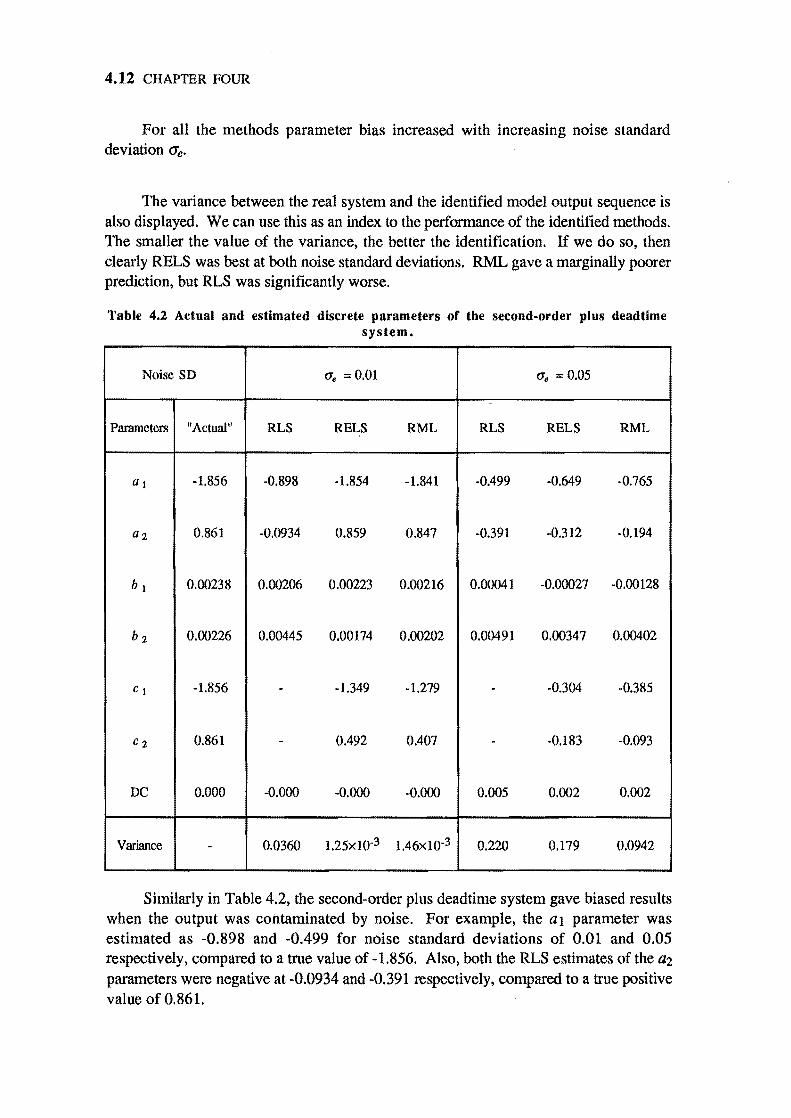
4.12 CHAPTER FOUR
For all the methods parameter bias increased with increasing noise standard deviation (ie.
The variance between the real system and the identified model output sequence is also displayed. We can use this as an index to the performance of the identified methods. The smaller the value of the variance, the better the identification. If we do so, then clearly RELS was best at both noise standard deviations. RML gave a marginally poorer prediction, but RLS was significantly worse.
Table 4.2 Actual and estimated discrete parameters of the second-order plus dead time system.
Noise SD (ie = 0.01 (ie = 0.05
Parameters "Actual" RLS RELS RML RLS RELS RML
a 1 -1.856 -0.898 -1.854 -1.841 -0.499 -0.649 -0.765
az 0.861 -0.0934 0.859 0.847 -0.391 -0.312 -0.194
b 1 0.00238 0.00206 0.00223 0.00216 0.00041 -0.00027 -0.00128
b z 0.00226 0.00445 0.00174 0.00202 0.00491 0.00347 0.00402
c 1 -1.856 - -1.349 -1.279 - -0.304 -0.385
Cz 0.861 - 0.492 0.407 - -0.183 -0.093
DC 0.000 -0.000 -0.000 -0.000 0.005 0.002 0.002
Variance - 0.0360 1.25xlO-3 1.46xlO-3 0.220 0.179 0.0942
Similarly in Table 4.2, the second-order plus deadtime system gave biased results when the output was contaminated by noise. For example, the al parameter was estimated as -0.898 and -0.499 for noise standard deviations of 0.01 and 0.05 respectively, compared to a true value of -1.856. Also, both the RLS estimates of the a2
parameters were negative at -0.0934 and -0.391 respectively, compared to a true positive value of 0.861.
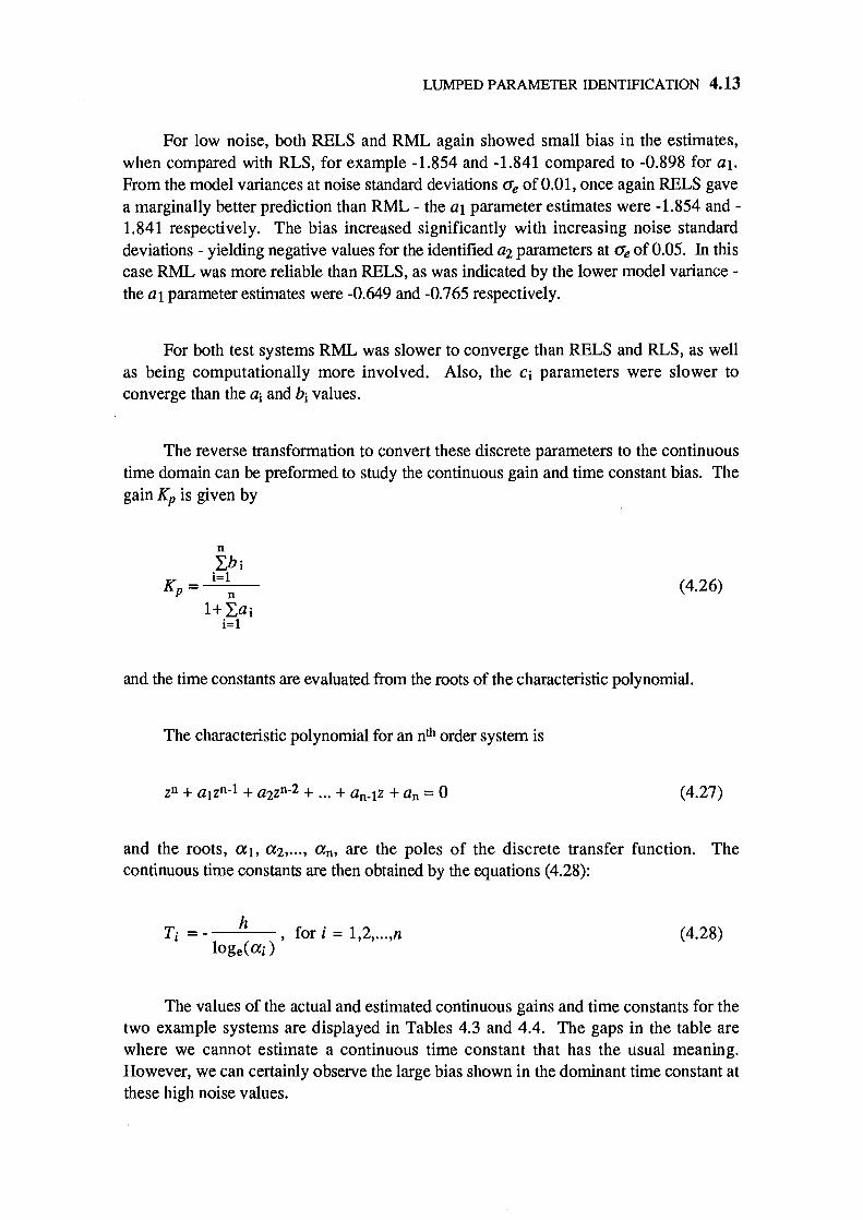
LUMPED PARAMETER IDENTIFICATION 4.13
For low noise, both RELS and RML again showed small bias in the estimates, when compared with RLS, for example -1.854 and -1.841 compared to -0.898 for al.
From the model variances at noise standard deviations ere of 0.01, once again RELS gave a marginally better prediction than RML - the al parameter estimates were -1.854 and -1.841 respectively. The bias increased significantly with increasing noise standard deviations - yielding negative values for the identified a2 parameters at ere of 0.05. In this case RML was more reliable than RELS, as was indicated by the lower model variance -the al parameter estimates were -0.649 and -0.765 respectively.
For both test systems RML was slower to converge than RELS and RLS, as well as being computationally more involved. Also, the Ci parameters were slower to converge than the ai and bi values.
The reverse transformation to convert these discrete parameters to the continuous time domain can be preformed to study the continuous gain and time constant bias. The gain Kp is given by
(4.26)
and the time constants are evaluated from the roots of the characteristic polynomial.
The characteristic polynomial for an nth order system is
(4.27)
and the roots, aI, a2, ... , an, are the poles of the discrete transfer function. The continuous time constants are then obtained by the equations (4.28):
h Tj = - ,
loge(aj) for i = 1,2, ... ,n (4.28)
The values of the actual and estimated continuous gains and time constants for the two example systems are displayed in Tables 4.3 and 4.4. The gaps in the table are where we cannot estimate a continuous time constant that has the usual meaning. However, we can certainly observe the large bias shown in the dominant time constant at these high noise values.
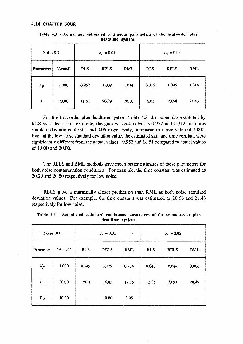
4.14 CHAPTER FOUR
Table 4.3 • Actual and estimated continuous parameters of the first-order plus dead time system.
Noise SD O'~ = 0.01 (f. = 0.05
Parameters "Actual" RLS RELS RML RLS RELS RML
Kp 1.000 0.952 1.008 1.014 0.312 1.005 1.016
T 20.00 18.51 20.29 20.50 6.05 20.68 21.43
For the first order plus deadtime system, Table 4.3, the noise bias exhibited by RLS was clear. For example, the gain was estimated as 0.952 and 0.312 for noise standard deviations of 0.01 and 0.05 respectively, compared to a true value of 1.000. Even at the low noise standard deviation value, the estimated gain and time constant were significantly different from the actual values - 0.952 and 18.51 compared to actual values of 1.000 and 20.00.
The RELS and RML methods gave much better estimates of these parameters for both noise contamination conditions. For example, the time constant was estimated as 20.29 and 20.50 respectively for low noise.
RELS gave a marginally closer prediction than RML at both noise standard deviation values. For example, the time constant was estimated as 20.68 and 21.43 respectively for low noise.
Table 4.4 • Actual and estimated continuous parameters of the second-order plus dead time system.
Noise SD O's = 0.01 0' .. = 0.05
Parameters "Actual" RLS RELS RML RLS RELS RML
Kp 1.000 0.749 0.779 0.734 0.048 0.084 0.066
Tl 20.00 126.1 16.83 17.85 12.36 33.91 28.49
T2 10.00 - 10.80 9.05 . - .
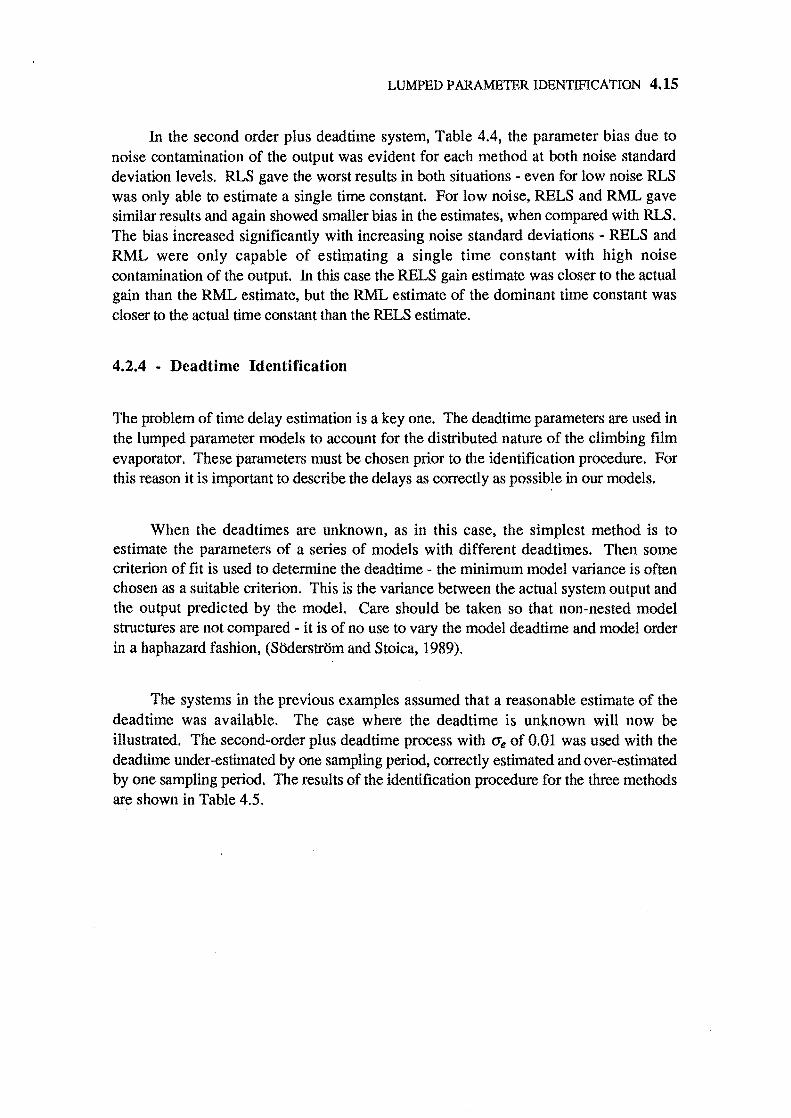
LUMPED PARAMETER IDENTIFICATION 4.15
In the second order plus deadtime system, Table 4.4, the parameter bias due to noise contamination of the output was evident for each method at both noise standard deviation levels. RLS gave the worst results in both situations - even for low noise RLS was only able to estimate a single time constant. For low noise, RELS and RML gave similar results and again showed smaller bias in the estimates, when compared with RLS. The bias increased significantly with increasing noise standard deviations - RELS and RML were only capable of estimating a single time constant with high noise contamination of the output. In this case the RELS gain estimate was closer to the actual gain than the RML estimate, but the RML estimate of the dominant time constant was closer to the actual time constant than the RELS estimate.
4.2.4 - Deadtirne Identification
The problem of time delay estimation is a key one. The deadtime parameters are used in the lumped parameter models to account for the distributed nature of the climbing film evaporator. These parameters must be chosen prior to the identification procedure. For this reason it is important to describe the delays as correctly as possible in our models.
When the deadtimes are unknown, as in this case, the simplest method is to estimate the parameters of a series of models with different deadtimes. Then some criterion of fit is used to determine the deadtime - the minimum model variance is often chosen as a suitable criterion. This is the variance between the actual system output and the output predicted by the model. Care should be taken so that non-nested model structures are not compared - it is of no use to vary the model deadtime and model order in a haphazard fashion, (SOderstrom and Stoica, 1989).
The systems in the previous examples assumed that a reasonable estimate of the deadtime was available. The case where the deadtime is unknown will now be illustrated. The second-order plus deadtime process with CTe of 0.01 was used with the deadtime under-estimated by one sampling period, correctly estimated and over-estimated by one sampling period. The results of the identification procedure for the three methods are shown in Table 4.5.
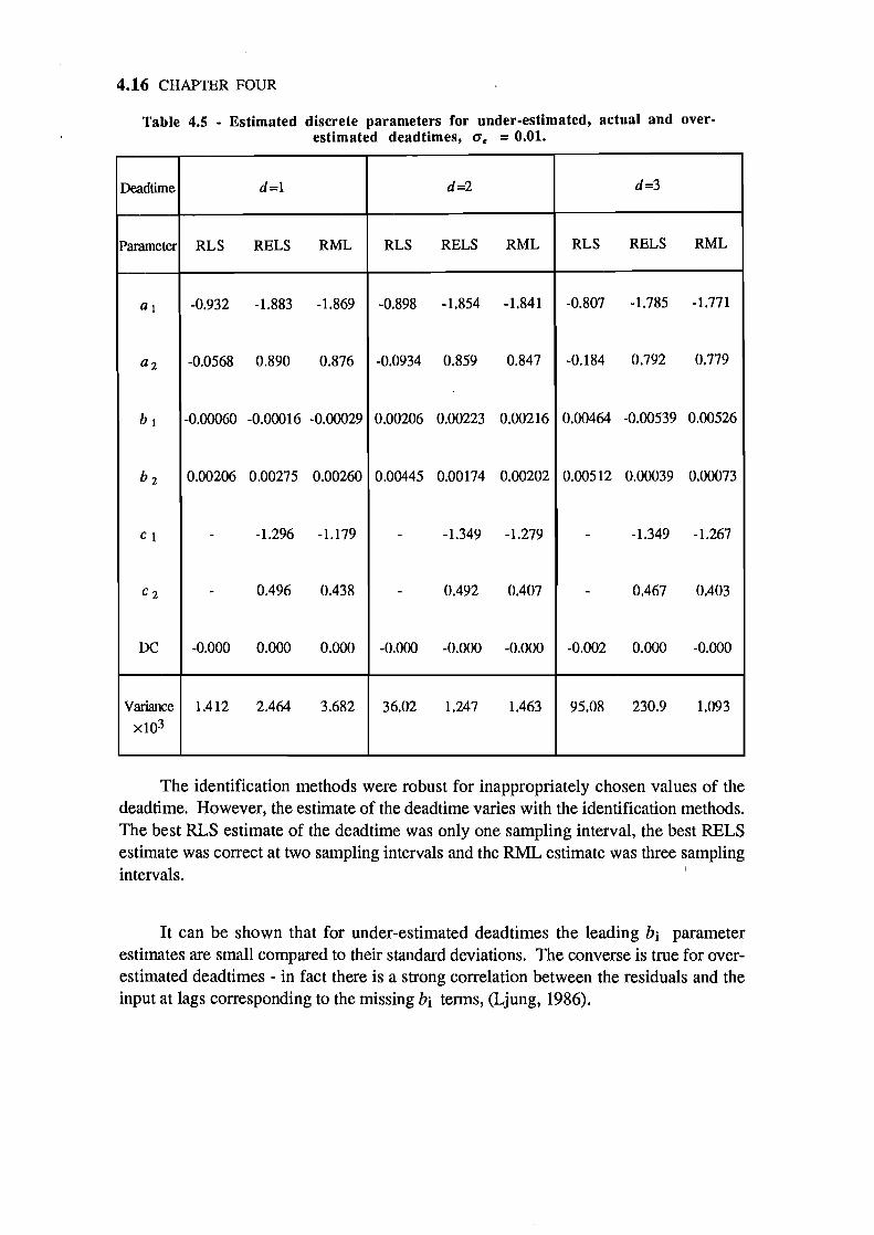
4.16 CHAPTER FOUR
Table 4.5 - Estimated discrete parameters for under-estimated, actual and overestimated deadtimes, (1, = 0.01.
Deadtime d=1 d=2 d=3
Parameter RLS RELS RML RLS RELS RML RLS RELS RML
a 1 -0.932 -1.883 -1.869 -0.898 -1.854 -1.841 -0.807 -1.785 -1.771
a2 -0.0568 0.890 0.876 -0.0934 0.859 0.847 -0.184 0.792 0.779
b 1 -0.00060 -0.00016 -0.00029 0.00206 0.00223 0.00216 0.00464 -0.00539 0.00526
b 2 0.00206 0.00275 0.00260 0.00445 0.00174 0.00202 0.00512 0.00039 0.00073
C1 - -1.296 -1.179 - -1.349 -1.279 - -1.349 -1.267
C2 - 0.496 0.438 - 0.492 0.407 - 0.467 0.403
DC -0.000 0.000 0.000 -0.000 -0.000 -0.000 -0.002 0.000 -0.000
Variance 1.412 2.464 3.682 36.02 1.247 1.463 95.08 230.9 1.093
x 103
The identification methods were robust for inappropriately chosen values of the deadtime. However, the estimate of the deadtime varies with the identification methods. The best RLS estimate of the deadtime was only one sampling interval, the best RELS estimate was correct at two sampling intervals and the RML estimate was three sampling intervals. I
It can be shown that for under-estimated dead times the leading hi parameter estimates are small compared to their standard deviations. The converse is true for overestimated deadtimes - in fact there is a strong correlation between the residuals and the input at lags corresponding to the missing hi terms, (Ljung, 1986).
LUMPED PARAMETER IDENTIFICATION 4.17
4.2.5 - Model Validation
Once a model structure has been chosen, such as ARMAX in this case, the problem of determining whether it is a good enough description of the process must be addressed. Model validation, or verification, is the process of testing whether a model is appropriate. for the intended purpose, and is at the heart of the identification procedure.
Validating a model has several aspects. Most model validation techniques concentrate on verifying if the model agrees sufficiently with the measurements of the system. Other questions to be addressed are whether the model is good enough for the user's purpose and if the model describes the "true system'" (Soderstrom and Stoica, 1989).
Bohlin (1987) suggests that to answer the questions above is to attack the model with as much information about the true system as is practicable - including a priori information, experimental observations and previous experience in using the particular model. In general when validating a model, one should run model simulations with the actual input data and perform cross-validation experiments with other input sequences. The approach taken here is to use the variance between the actual system output and the predicted model output. Plots of the actual system output and the identified model output versus time may also be visually examined for a qualitative comparison.
4.2.6 - Identification of MISO Models
The models identified in sections 4.2.3 and 4.2.4 have been of single-input, singleoutput (SISO) form. The recursive algorithms can be simply extended to perform multiinput, single-output (MISO) identification. A multi-input, multi-output (MIMO) model can then be constructed from a series of MISO models.
Two methods of recursive identification, RLS and RELS, were compared by application to sets of data simulated from a MISO test system. RML was not used because of its higher computational cost. The input signals {Ui(k)} were chosen to be pseudo random binary sequences of character N(O,O.I) (zero mean with standard deviation of 0.1), with step changes of unity magnitude and minimum periods equal to the sampling period.
The test system was MISO first-order plus dead time in the continuous-time domain. The system was transformed to find the discrete-equivalents in the z-plane by determining the zero-order hold equivalences.
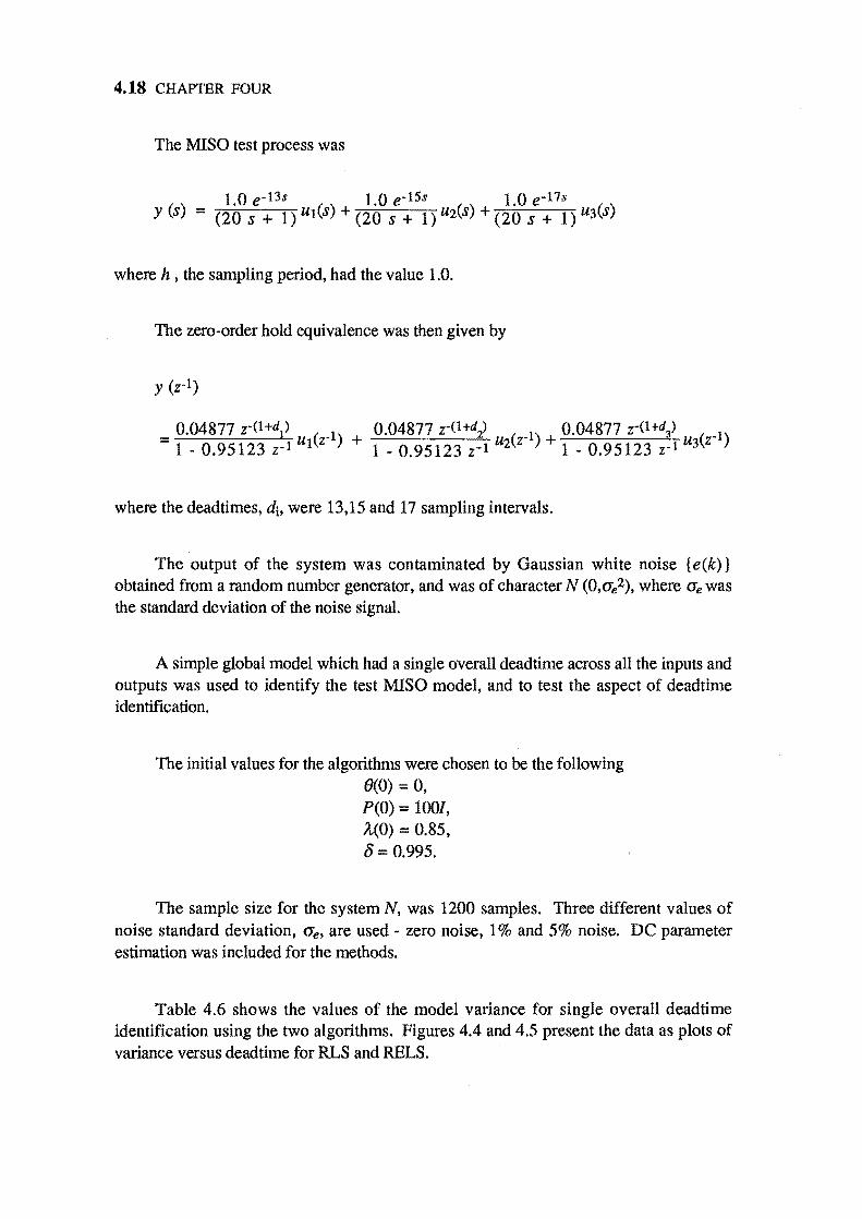
4.18 CHAPTER FOUR
The MISO test process was
y (s)
where h , the sampling period, had the value 1.0.
The zero-order hold equivalence was then given by
Y (z-l)
where the deadtimes, dh were 13,15 and 17 sampling intervals.
The output of the system was contaminated by Gaussian white noise (e(k)} obtained from a random number generator, and was of character N (0,O"e2), where O"e was the standard deviation of the noise signal.
A simple global model which had a single dverall deadtime across all the inputs and outputs was used to identify the test MISO model, and to test the aspect of deadtime identification.
The initial values for the algorithms were chosen to be the following 0(0) = 0, P(O) = 100/, IL(O) = 0.85, a = 0.995.
The sample size for the system N, was 1200 samples. Three different values of noise standard deviation, O"e, are used - zero noise, 1 % and 5% noise. DC parameter estimation was included for the methods.
Table 4.6 shows the values of the model variance for single overall deadtime identification using the two algorithms. Figures 4.4 and 4.5 present the data as plots of variance versus dead time for RLS and RELS.
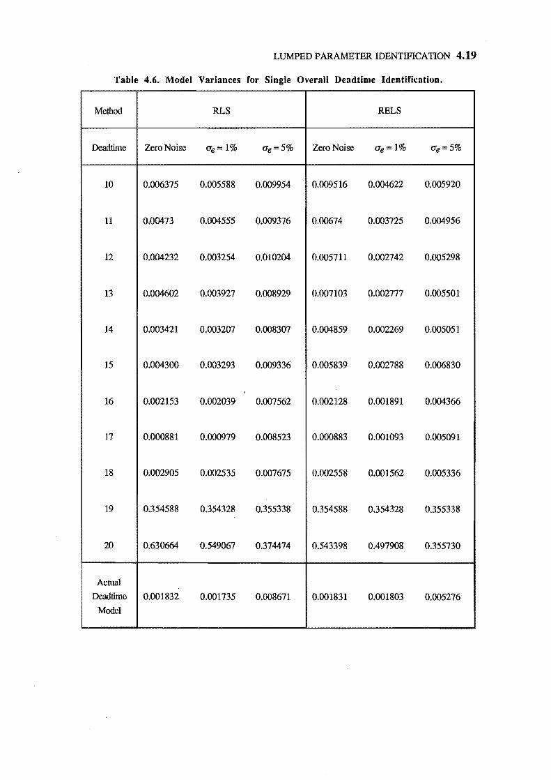
LUMPED PARAMETER IDENTIFICATION 4.19
Table 4.6. Model Variances for Single Overall Deadtime Identification.
Method RLS RELS
Deadtime Zero Noise O"e = 1% O"e = 5% Zero Noise O"e = 1% O"e= 5%
10 0.006375 0.005588 0.009954 0.009516 0.004622 0.005920
11 0.00473 0.004555 0.009376 0.00674 0.003725 0.004956
12 0.004232 0.003254 0.010204 0.005711 0.002742 0.005298
13 0.004602 0.003927 0.008929 0.007103 0.002777 0.005501
14 0.003421 0.003207 0.008307 0.004859 0.002269 0.005051
15 0.004300 0.003293 0.009336 0.005839 0.002788 0.006830
I
16 0.002153 0.002039 0.007562 0.002128 0.001891 0.004366
17 0.000881 0.000979 0.008523 0.000883 0.001093 0.005091
18 0.002905 0.002535 0.007675 0.002558 0.001562 0.005336
19 0.354588 0.354328 0.355338 0.354588 0.354328 0.355338
20 0.630664 0.549067 0.374474 0.543398 0.497908 0.355730
Actual
Deadtime 0.001832 0.001735 0.008671 0.001831 0.001803 0.005276
Model
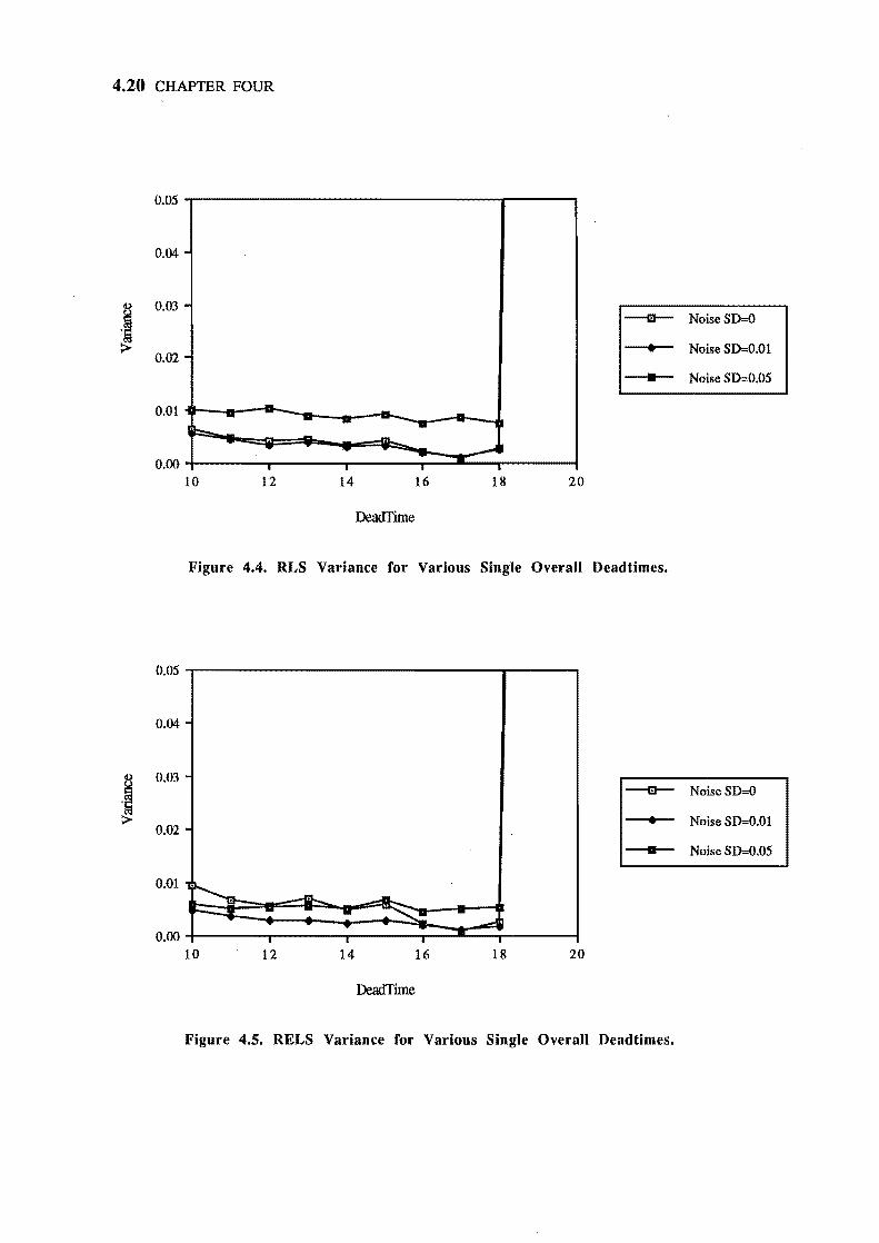
4.20 CHAPTER FOUR
0.05
0.04 -
0.03 ----m-- Noise SO=O
0.02 • Noise SI>=O.o1
• Noise S1>=0.05
--- .... - .... b..
~- .... --. 0.01
-- ..r.L .... ... --- .....,..-I ..... • • 0.00
10 12 14 16 18 20
DeadTime
Figure 4.4. RLS Variance for Various Single Overall Deadtimes.
0.05
0.04 -
<I) 0.03 -
.~ :>
0.Q2 -
---m-- Noise SD=O
• Noise SI>=O.OI
a Noise SO=O.05
0.01 , .~ -m.. -II. .... - ~ 'Y .......d
0.00 • • 10 12 14 16 18 20
DeadTime
Figure 4.5. RELS Variance for Various Single Overall Deadtimes.
LUMPED PARAMETER IDENTIFICATION 4.21
For low noise (Zero and 1 %) the dominant deadtime is the largest value, i.e. 17 sampling intervals (equal the value of d3). For higher noise (5%) the best model is for a single overall deadtime of 16 sampling intervals, (between the values of d2 and d3). Table 4.7 details the identified time constants for these deadtimes and also for the actual model deadtimes.
Table 4.7 Identified Time Constants for the Actual Deadtime Models and the Best Single Overall Deadtime Models.
Method RLS RELS
Deadtime Zero Noise O'e = 1% O'e= 5% Zero Noise O'e = 1% O'e = 5%
Actual 20.000 19.492 10.525 20.00 19.177 15.302
Single 19.321 18.902 12.226 19.341 19.313 19.364
Clearly the parameter bias increases with increasing noise contamination. As expected, RELS demonstrates less bias than RLS for high noise (5%).
The single overall deadtime models estimated the time constant well, even though the deadtime model was incorrect.
4.2.7 - Conclusions
The RLS method returned biased parameter estimates for cases where there was any noise contamination of the output.
RELS and RML reduced but did not eliminate parameter bias. Both RELS and RML gave reasonable parameter estimates at low noise standard deviations, but the parameter estimates deteriorated for higher noise values. RML was marginally better than RELS at estimating the dominant time constant in these cases.
RML was slower to converge than RELS and RML. It required RLS initialisation and more computation than the other two methods.
The identification methods were robust for inappropriate choices of deadtime. For the SISO models the actual deadtime could be inferred from the RELS method.
4.22 CHAPTER FOUR
For MISO model identification with RLS and RELS, the parameter bias increased with increasing noise contamination. As expected, RELS demonstrated less bias than RLS for higher noise contamination.
The MISO single overall deadtime models were capable of identifying the dominant deadtime, although this ability deteriorated with higher noise contamination. The estimated the time constant was also close to the true value, even though the assumed deadtime model was incorrect.
Overall it seems that the recursive lumped parameter methods, although fine for no noise, give poor results for any noise contamination - which occurs in any real system. There may be scope here for the development of some better methods.
ABBREVIATIONS
ARX AutoRegressive, Exogeneous variable
ARMAX AutoRegressive Moving Average, Exogeneous variable
RLS Recursive Least Squares
RELS Recursive Extended Least Squares
RML Recursive Maximum Likelihood
SYMBOLS
A= [al ... an] Output parameter vector
B = [bi ... bn] Input parameter vector
c = [Cl ..• en] Noise model parameter vector
d Deadtime, expressed in sampling intervals
DC Additional parameter for regression of absolute variables
e(k) White noise sequence
G(s) Laplace transfer function
i "Dummy" variable
k kth time instant
Kp
L(k)
P(k)
n
s
T;
u(k)
U(k)
v(k)
y(k)
Y(k)
z
o
;t(k)
((i..k)
4I(k)
~k)
O'e
LUMPED PARAMETER IDENTIFICATION 4.23
Process gain
UD factorisation gain vector
Regression error covariance matrix
Model order
Delay or backward shift operator
Laplace variable
Time
Time constant i
Input deviation variable
Input absolute variable
Input steady state value
Equation error
Output deviation variable
Output absolute variable
Output steady state value
Discrete transfonn operator
A constant for forgetting factor determination
Forgetting factor
Regression vector
Filtered data or gradient vector for RELS and RML
Regression parameter vector
Noise standard deviation
4.24 CHAPTER FOUR
REFERENCES
Astrom, K.J. and Bohlin, T., "Numerical Identification of linear dynamic systems from
normal operating records", IFAC Symposium on Theory of Self-Adaptive Control Systems,
Teddington, England (1965).
Biermann, G.J., "Factorisation Methods for Discrete Sequential Estimation",
Academic Press (1977).
Bohlin, T., "Model Validation", In "Encyclopedia of Systems and Contro!", (M.Singh, Ed.),
Pergamon Press (1987).
Franklin, G.F. and Powell, J.D., "Digital Control of Dynamic Systems",
Addison-Wesley (1980).
Goodwin, G.C. and Sin, K.S., "Adaptive filtering prediction and control",
Prentice-Hall (1984).
Hsia, T.C., "System Identification", Lexington Books (1971).
Isermann, R., "Comparison and Evaluation of 6 On-line Identification and Parameter
Estimation Methods with 3 Simulated Processes", Proc. Symp. on Identification and Parameter
Estimation, The Hague/Delft, The Netherlands, Pergamon Press, (1973).
Ljung, L., "System Identification - Theory for the User", Prentice-Hall (1987).
Ljung, L., "System Identification Toolbox for use with MATLAB. User's Guide",
The MathWorks, Inc., (1986).
Ljung, L. and Soderstrom, T., "Theory and Practice of Recursive Identification",
MIT Press (1983).
Soderstrom, T. and Stoica, P., "System Identification", Prentice Hall, (1989).
CHAPTER
FIVE
DISTRIBUTED PARAMETER SYSTEMS IDENTIFICATION
In which methods for the identification of distributed parameter systems are surveyed.
5.1 • INTRODUCTION
As noted in Chapter 5, the climbing film evaporator, along with many other industrial processes, is a distributed parameter system, characterised by the fact that the system states, inputs and outputs may depend on spatial position as well as time. In this case, the spatial variable is the length of the evaporator tube.
The two general approaches taken in the modelling, identification and control of distributed parameter systems are the lumped parameter approach and the distributed parameter approach.
The second approach is application of the modelling, identification and control theory for distributed parameter systems. It is only after the final controller design that the process is lumped for implementation of the control procedures. These identification methods are examined in this chapter.
5.2 - DISTRIBUTED PARAMETER SYSTEMS
As has been already discussed, there is a major body of work that is concerned with the identification of lumped parameter systems described by ordinary differential equations. The assumption is that distributed phenomena may be approximated adequately by a lumped parameter model - the local spatial variations are ignored and the system in question is considered to be homogeneous. Whether the lumped parameter model is valid or not is not easily determined. If the system response shows instantaneous variation along a spatial coordinate, a distributed parameter model should be considered.
5.1

5.2 CHAPTER FIVE
Polis and Goodson (1976), Kubrusly (1977) and Polis (1982) survey the methods used in distributed parameter system identification and Ray (1978) presents a survey of applications of distributed parameter system theory.
A number of difficulties arise with distributed parameter system identification that are not usually found with lumped systems. The difficulties are provided by the infinite dimensional space - the parameter space may be infinite dimensional and the location and type of measurement sensors must be chosen appropriately.
Polis (1976, 1982) breaks the distributed parameter identification problem into a number of subproblems:
1 . The mathematical description of the process under consideration must be written. This will be a system of partial differential equations containing the unknown parameters that are to be determined.
2. A method of solution for the partial differential equations must be chosen.
3 . A performance criterion is chosen.
4. The measurement location and type must be decided.
5. The data is obtained by performing an experiment.
6. An optimisation scheme is chosen to identify the unknown parameters of the partial differential equations describing the system.
In order to identify a distributed parameter system each of the previous steps must be considered in turn.
DISffilBUTED PARAMETER IDENTIFICATION 5.3
The chosen mathematical model describing the climbing evaporator was a set of hyperbolic differential equations. The method of characteristics was selected as a solution method, to take advantage of the hyperbolic nature of these equations. The perfOlmance criterion of choice for the identification scheme was the output least square error criterion - in common with most researchers and also lumped parameter modelling (Polis, 1982). The measurements that were available for the identification are detailed in Chapter 2. The bulk of work on the distributed identification problem uses gradientbased off-line optimisation schemes. In particular, Carpenter et al (1971) detail the solution of distributed parameter systems described by hyperbolic partial differential equations using the method of characteristics. This method was adapted to the identification of simplified distributed parameter models of the climbing film evaporator.
The Method of Characteristics
The method of characteristics, section 3.3, may be used to obtain exact solutions for hyberbolic systems. To illustrate the method, the process described by the following hyperbolic partial differential equation was investigated
aU(X,t) + au(x,t) + b ( t) - 0 at a ax U x, -
where a and b are constants.
The hyberbolic partial differential equation has the characteristic equations
dx dt =a
and du dt = -bu
Two spatial measurements of u(x,t) at locations Xl and X2 are required. The characteristic equations may then be used to extend the measurement at (Xt,tl) to the second measurement point (x2h). The predicted value of U at this point is given by
where the equivalent lumped time delay is
5.4 CHAPTER FIVE
The predicted value may then be compared with the actual value at (X2,t2), a prediction error criterion formed and the values of a and/or b are chosen to minimise the error criterion.
For example, for the identification of b, the error criterion may be defined as
N
J(b) =i L{[u(t) - u(t - Td)e-bTd]2} i=l
Carpenter et al (1971) used a stochastic approximation algorithm to yield a and b parameter estimates. The stochastic approximation method is simply a gradient method used in a stochastic environment and may be applied to a system of partial differential equations.
Malpani and Donnelly (1972, 1973) have also used the method of characteristics for the identification of hyperbolic distributed parameter systems.
Implementation
For a hyperbolic distributed parameter model, the least squares estimation algorithm of Levenberg-Marquardt (Vetterling et aI., 1986) was chosen as the optimisation scheme. The program MRQFIT.FOR on the floppy disk labelled "PROGRAMS" contains the VAX-FORTRAN source code for this method.
SYMBOLS
a,b Constant parameters of the partial differential equation
J(b) Prediction error criterion, with respect to the parameter b
Time
T d Time delay
u(x,t) State variable
x Distance
'r Time constant
Subscripts
1 Spatial position 1
2 Spatial position 2
DISTRIBUTED PARAMETER IDENTIFICATION 5.5
REFERENCES
Carpenter, W.T., Wozny, M.J. and Goodson, R.E., "Distributed Parameter
Identification Using the Method of Characteristics", Trans. AS ME, J. Dynamic Systems,
Measurement and Control, Vol. 93, pp73-78 (1971).
Kubrusly, C.S., "Distributed parameter system identification. A survey", Int. J. Control,
Vol.26, No.4, pp509-535 (1977).
Logan, J.D., "Applied Mathematics. A Contemporary Approach", Wiley-Interscience,
pp248-249 (1987).
Malpani, S.N. and Donnelly, J.K., "Identification of One Phase Flow Processes",
Can. J. Chem. Eng., Vol. 50, pp791-795 (1972).
Malpani, S.N. and Donnelly, J.K., "Identification of a Packed Absorption Column",
Can. J. Chern. Eng., Vol. 51, pp479-483 (1973).
Polis, M.P., "The Distributed System Parameter Identification Problem: A Survey of Recent
Results", Proc. 3rd IFAC Symp. on Control of Distributed Parameter Systems, Tolouse, France,
pp45-58 (1982).
Polis, M.P. and Goodson, R.E., "Parameter Identification in Distributed Systems:
A Synthesizing Overview", IEEE Proceedings, Vol. 64, No.1, January (1976).
Ray, W.H., "Some Recent Applications of Distributed Parameter Systems Theory - A Survey",
Automatica, Vo1.14, pp281-287 (1978).
Vetterling, W.T., Teukolsky, S.A., Press, W.H. and Flannery, B.P., "Numerical
Recipes", Cambridge University Press, (1986).

CHAPTER
SIX
DATA COLLECTION AND IDENTIFICATION STRATEGY
In which the design of the data collection experiments are presented and the overall identification procedure is outlined.
6.1 DATA COLLECTION
The form of the evaporator model which was to be identified, using the methods described in chapter 4 and chapter 5, was linear multi-input multi-output (MIMO). The model structure is described by the block diagram in Figure 6.1.
iables Input Var
ul -.. ... ...
Oulpu t Variables
... EVAPORATOR
MODEL ... G --... ...,
--..
Figure.6.1. Block Diagram for the linear MIMO Model of the Climbing Film Evaporator.
6.1
6.2 CHAPTER SIX
For the model of the climbing film evaporator described by Figure 6.1 the input variables were
Ul = steam temperature in the steam jacket on the evaporator tube. U2 = feed flowrate to the evaporator, u3 = temperature of the evaporator feed, U4 = concentration of the evaporator feed,
and the output variables were
Yl = concentration of the product concentrate, Y2 = exit flowrate of the product concentrate, Y3 = temperature of the product concentrate, Y4 = concentration of the product condensate.
The identification methods used to identify the parameters of the model of the above structure required a reasonable number of samples before the parameter estimates converged to their final values from the initial guesses. The number of samples was chosen to be 1000 samples of all the input and output variables at an instant of time. The choice of sample rate was important so that undesirable effects such as aliasing were avoided, (Astrom and Wittenmark, 1984). The sample rate chosen was one sample every 12 seconds, small enough to avoid aliasing problems yet sufficiently large to overcome measurement delays. An experiment duration of 3 hours 20 minutes to collect 1000 . samples was implied.
The experiments performed took the form of two 23 factorial experiments (Montgomery, 1984) with a single replicate, at two different input feed temperatures. An independent pseudorandom binary sequence or PRBS (SOderstrom and Stoica, 1989) was superimposed on each of the following inputs - steam temperature, feed flowrate and feed concentration. These inputs were varied independently of each other. The PRBS on the steam temperature was obtained by altering the steam flowrate to the steam jacket on the evaporator tube. The PRBS on the feed concentration was afforded by switching between the two feed tanks which contained solutions of two different concentrations.
The above constraints lead to two experiments consisting of four blocks/trials each consisting of four runs at a particular operating points. These runs were randomised within each trial. The duration of each run was 8 hours - determined by the feed flowrate and feed tank capacity. This resulted in 19200 measurements of four input and four output variables for the identification of the selection of models of the evaporator.

DATA COLLECTION AND IDENTIFICATION STRATEGY 6.3
A separate set of data is desirable for verification purposes. Two verification experiments at different feed temperatures were performed. The input signal to the plant was a sequence of operating points. The plant was held steady at each point for 15 minutes, before switching to the next operating point. A run duration of 4 hours resulted in a total of 2400 points for the two verification experiments.
The advantage of this rigourous design of the data collection experiments is that it provides a systematic basis for comparison of the various identification methods and models to be studied.
6.2 OVERALL IDENTIFICATION STRATEGY
Simple models of the climbing film evaporator may not be adequate to describe the behaviour or more complex models may give better predictions. The identification strategy pursued was to consider each of the following models in turn and compare and contrast the results.
• A "simple" global model - ranging from a first order model to higher order models.
• A series of simple linear models at each individual operating point.
• Distributed parameter models.
The first two sets of models are all examples of lumped parameter models of the evaporator and the methods of chapter 4 can be applied to the climbing film evaporator data. The techniques of chapter 5 are then used to identify distributed parameter models of the evaporator.
The basis of the comparison was chosen as the variance of the output errors. The variances were normalised by the span of the output variable concerned so that the predictions for different outputs could be compared directly.
ABBREVIATIONS
MIMO Multi-Input, Multi-Output
PRBS PseudoRandom Binary Sequence
6.4 CHAPTER SIX
SYMBOLS
u 1 steam temperature in the steam jacket on the evaporator tube
U2 feed flowrate to the evaporator
Ug temperature of the evaporator feed
U4 concentration of the evaporator feed
Y 1 concentration of the product concentrate,
Y2 exit flowrate of the product concentrate
yg temperature of the product concentrate
y 4 concentration of the product condensate
REFERENCES
Astrom, K.J. and Wittenmark, B., "Computer Controlled Systems: Theory and Design",
Prentice-Hall International, pp25-27,pp405-7 (1984).
Montgomery, D.C., "Design and Analysis of Experiments", 2nd Ed., Wiley, pp186-191 (1984).
S6derstrom,T. and Stoica,P., "System Identification", Prentice Hall, pp96-145 (1989).
CHAPTER
SEVEN
GLOBAL LUMPED PARAMETER MODELS
In which the lumped identification procedures outlined in chapter 4 are applied to global models of the climbing film evaporator. The resulting identified models are presented and discussed.
7.1 A "simple" global model of the Evaporator
The simplest global model of the climbing film evaporator investigated was one which had a single overall deadtime across all the inputs and outputs, and equal model orders. The model was easily extended to the case with a single overall dead time. but with the best combination of model orders. The further case where the four multi-input, singleoutput (MISO) systems were considered separately was also investigated. Overleaf Figure 7.1 presents the MISO models in block diagram form, with model order unity.
7.1
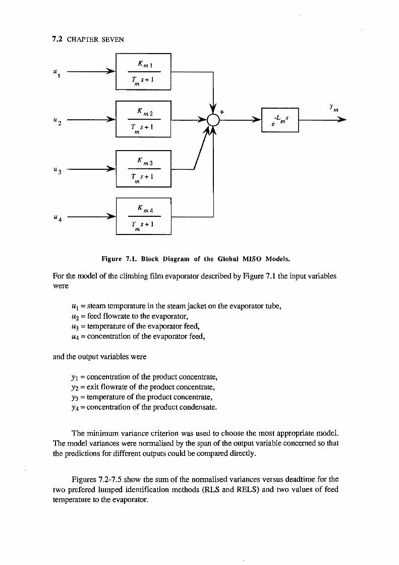
7.2 CHAPTER SEVEN
Kml
" T s+ 1 m
Km2 ,~
,,"" + Ym
'" '" -L s ,. , ~ e m
T s+ 1 m V~
'" Km3
... T s+ 1
m
" Km4
, T s+ 1
m
Figure 7.1. Block Diagram of the Global MISO Models.
For the model of the climbing film evaporator described by Figure 7.1 the input variables were
Ul = steam temperature in the steam jacket on the evaporator tube, u2 = feed flowrate to the evaporator, u3 = temperature of the evaporator feed, U4 = concentration of the evaporator feed,
and the output variables were
Yl = concentration of the product concentrate, Y2 = exit flowrate of the product concentrate, Y3 = temperature of the product concentrate, Y 4 = concentration of the product condensate.
"
The minimum variance criterion was used to choose the most appropriate model. The model variances were normalised by the span of the output variable concerned so that the predictions for different outputs could be compared directly.
Figures 7.2-7.5 show the sum of the normalised variances versus deadtime for the two prefered lumped identification methods (RLS and RELS) and two values of feed temperature to the evaporator.
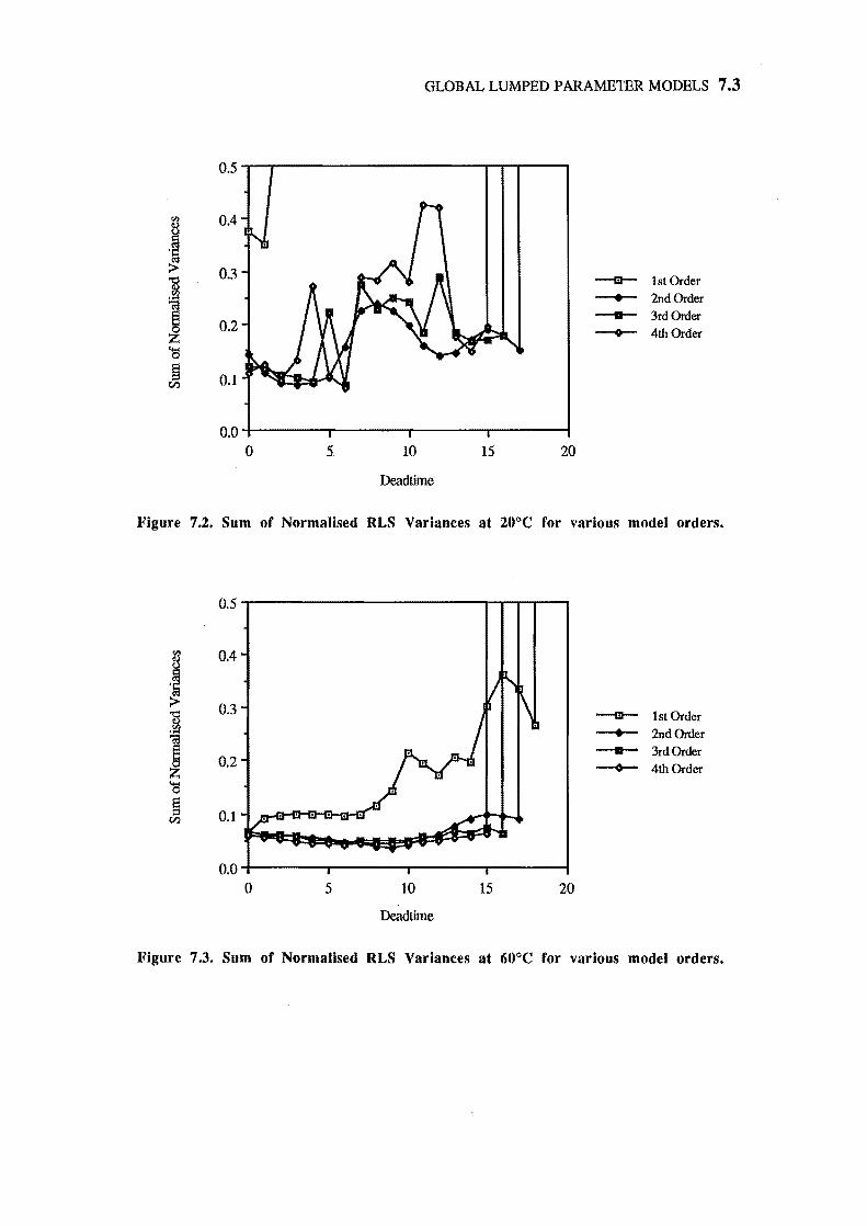
GLOBAL LUMPED PARAME1ER MODELS 7.3
0.5
r;) 0.4 ~
.~ ::> 0.3
1 --m- 1st Order
--+- 2nd Order ---- 3rdOrder 0.2 --+-- 4th Order Z
'Cl § 0.1 en
0.0 0 5. 10 15 20
Deadtime
Figure 7.2. Sum of Normalised RLS Variances at 20°C for various model orders.
0.5
~ 0.4
.~ ::> 0.3
i --m- 1st Order
--+- 2nd Order
~ ---- 3rdOrder 0.2 --0- 4th Order
..... 0
§ 0.1 en
0.0 0 5 10 15 20
Deadtime
Figure 7.3. Sum of Normalised RLS Variances at 60°C for various model orders.
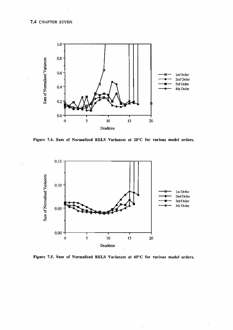
7.4 CHAPTER SEVEN
1.0
8 .!
0.8
> 0.6 ] Ill-- 1st Order
1 • 2nd Order a 3rdOrder
0.4 ~ ~ 4th Order
~
~ til
0.0 0 5 10 15 20
Deadtime
Figure 7.4. Sum of Normalised RELS Variances at 20°C for various model orders.
0.15 -r--------------r'-r-r----,
8 .! >
0.10
] ---a- 1st Order
~ • 2nd Order
~ a 3rd Order ~ 4th Order
~ 0.05
~ til
0.00 -t----.------;.------r----I
o 5 10 15 20
Deadtime
Figure 7.5. Sum of Normalised RELS Variances at 60°C for various model orders.
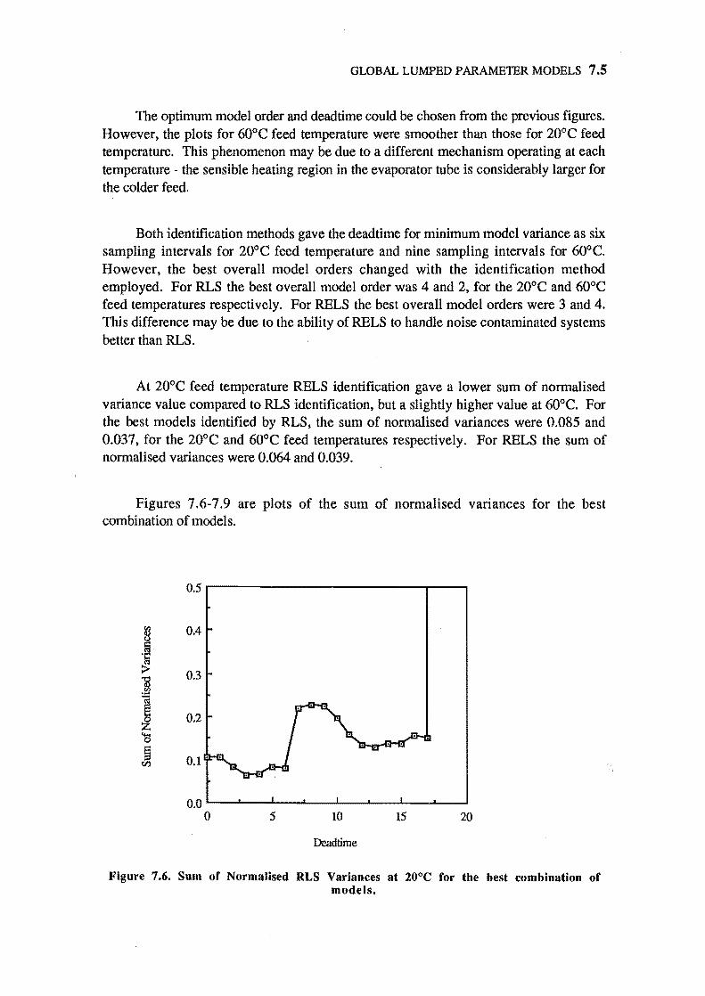
GLOBAL LUMPED PARAMETER MODELS 7.5
The optimum model order and dead time could be chosen from the previous figures. However. the plots for 60°C feed temperature were smoother than those for 20°C feed temperature. This phenomenon may be due to a different mechanism operating at each temperature - the sensible heating region in the evaporator tube is considerably larger for the colder feed.
Both identification methods gave the deadtime for minimum model variance as six sampling intervals for 20°C feed temperature and nine sampling intervals for 60°C. However, the best overall model orders changed with the identification method employed. For RLS the best overall model order was 4 and 2, for the 20°C and 60°C feed temperatures respectively. For RELS the best overall model orders were 3 and 4. This difference may be due to the ability of RELS to handle noise contaminated systems better than RLS.
At 20°C feed temperature RELS identification gave a lower sum of normalised variance value compared to RLS identification, but a slightly higher value at 60°C. For the best models identified by RLS, the sum of normalised variances were 0.085 and 0.037, for the 20°C and 60°C feed temperatures respectively. For RELS the sum of normalised variances were 0.064 and 0.039.
Figures 7.6-7.9 are plots of the sum of normalised variances for the best combination of models.
0.5
8 .~
0.4
:>- 0.3
t 0.2 ~ 'Cl §
0.1 .. V)
0.0 0 5 10 15 20
Deadtime
Figure 7.6. Sum of Normalised RLS Variances at 20°C for the best combination of models.
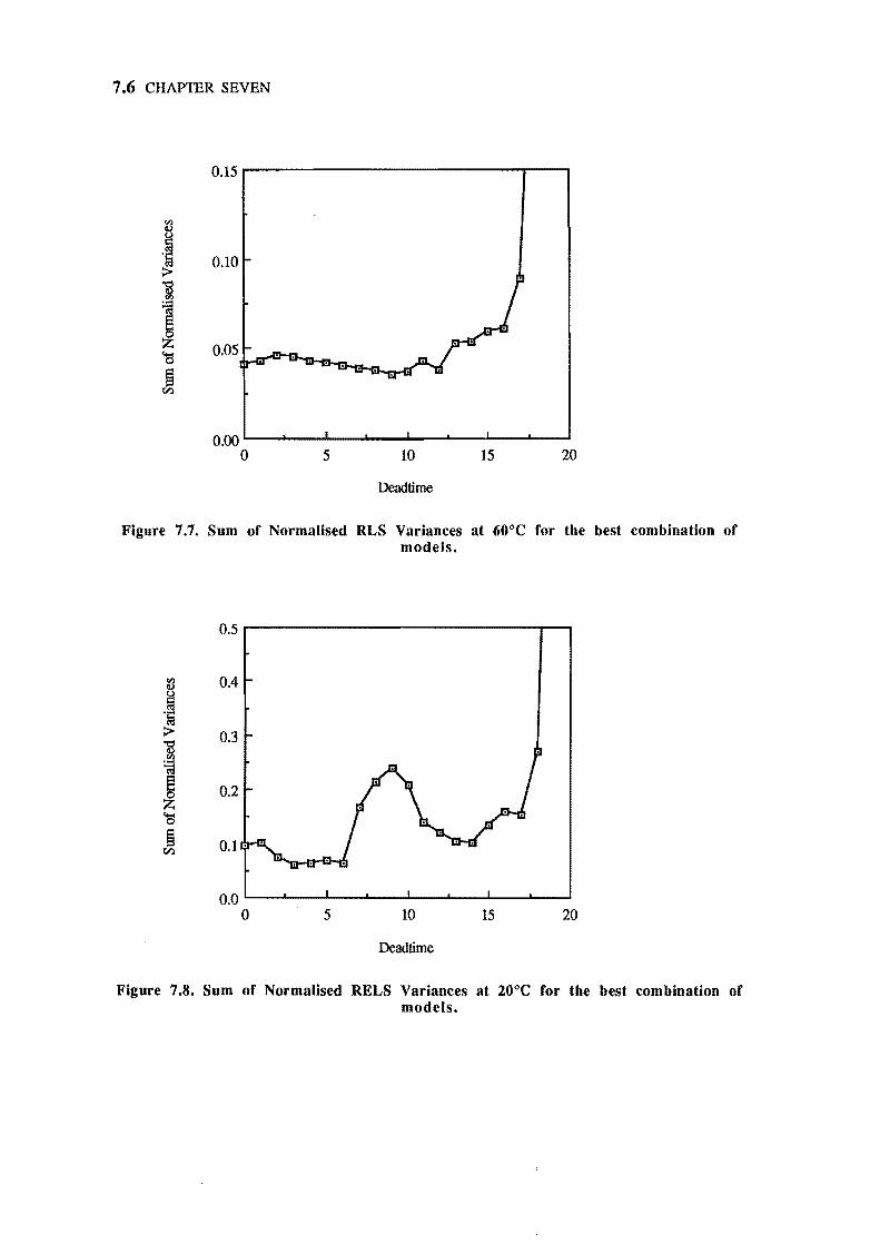
7.6 CHAPTER SEVEN
0.15,...---------------r----,
0.10
0.05
0.00 1...----1_---1_--&._......1.._---'-_-1...._-'-----1
o 5 10 15 20
Deadtime
Figure 7.7. Sum of Normalised RLS Variances at 60°C for the best combination of models.
0.5
~ 0.4
·i > 0.3
~ ~ Z
0.2
'Cl @ til
0.0 0 5 10 15 20
Deadtime
Figure 7.S. Sum of Normalised RELS Variances at 20°C for the best combination of models.
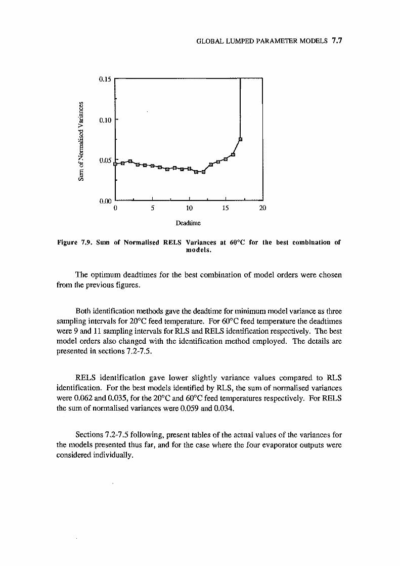
GLOBAL LUMPED PARAMETER MODELS 7.7
0.15 .---------------...r---..,
0.10
0.00 L..-.........I_......I._--L_--I.._-'-_....I-_-'-----I
o 5 10 15 20
Deadtime
Figure 7.9. Sum of Normalised RELS Variances at 60°C for the best combination of models.
The optimum dead times for the best combination of model orders were chosen from the previous figures.
Both identification methods gave the dead time for minimum model variance as three sampling intervals for 200 e feed temperature. For 600 e feed temperature the deadtimes were 9 and 11 sampling intervals for RLS and RELS identification respectively. The best model orders also changed with the identification method employed. The details are presented in sections 7.2-7.5.
RELS identification gave lower slightly variance values compared to RLS identification. For the best models identified by RLS, the sum of normalised variances were 0.062 and 0.035, for the 200 e and 600 e feed temperatures respectively. For RELS the sum of normalised variances were 0.059 and 0.034.
Sections 7.2-7.5 following, present tables of the actual values of the variances for the models presented thus far, and for the case where the four evaporator outputs were considered individually.
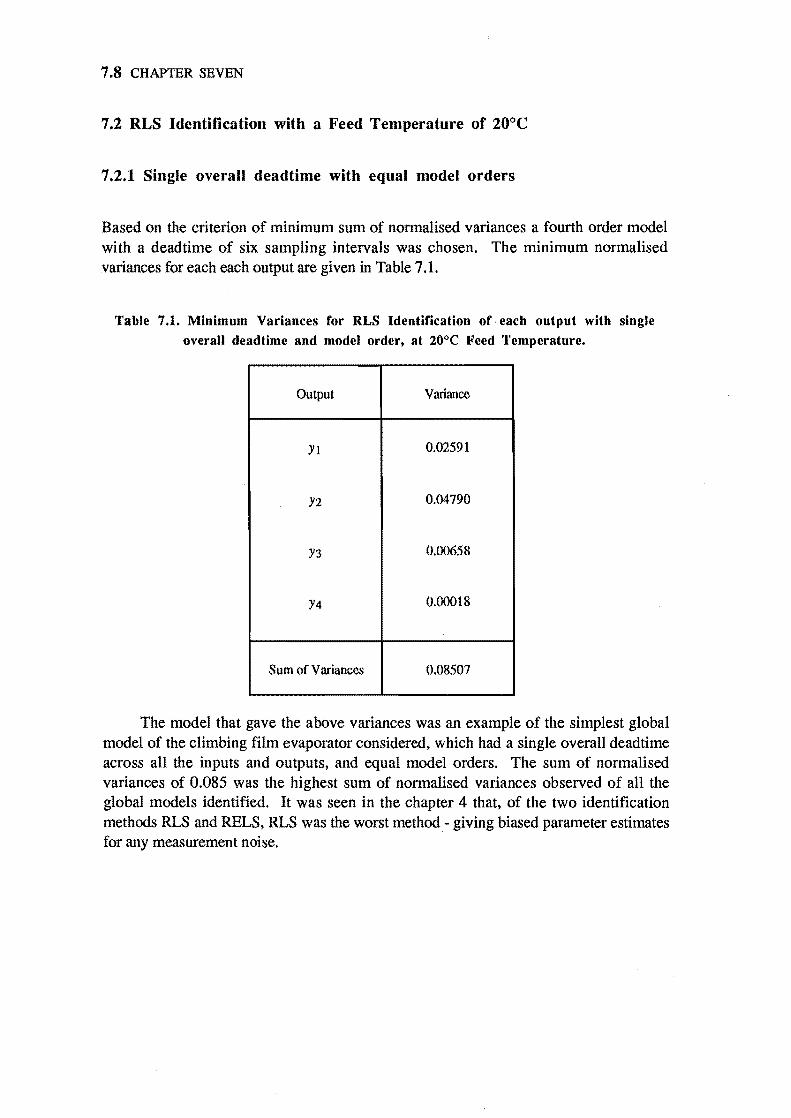
7.8 CHAPTER SEVEN
7.2 RLS Identification with a Feed Temperature of 20°C
7.2.1 Single overall deadtime with equal model orders
Based on the criterion of minimum sum of normalised variances a fourth order model with a deadtime of six sampling intervals was chosen. The minimum normalised variances for each each output are given in Table 7.1.
Table 7.1. Minimum Variances ror RLS Identirication or, each output with single overall dead time and model order, at 20°C Feed Temperature.
Output Variance
Yl 0.02591
Y2 0.04790
Y3 0.00658
Y4 0.00018
Sum of Variances 0.08507
The model that gave the above variances was an example of the simplest global model of the climbing film evaporator considered, which had a single overall deadtime across all the inputs and outputs, and equal model orders. The sum of normalised variances of 0.085 was the highest sum of normalised variances observed of all the global models identified. It was seen in the chapter 4 that, of the two identification methods RLS and RELS, RLS was the worst method - giving biased parameter estimates for any measurement noise.
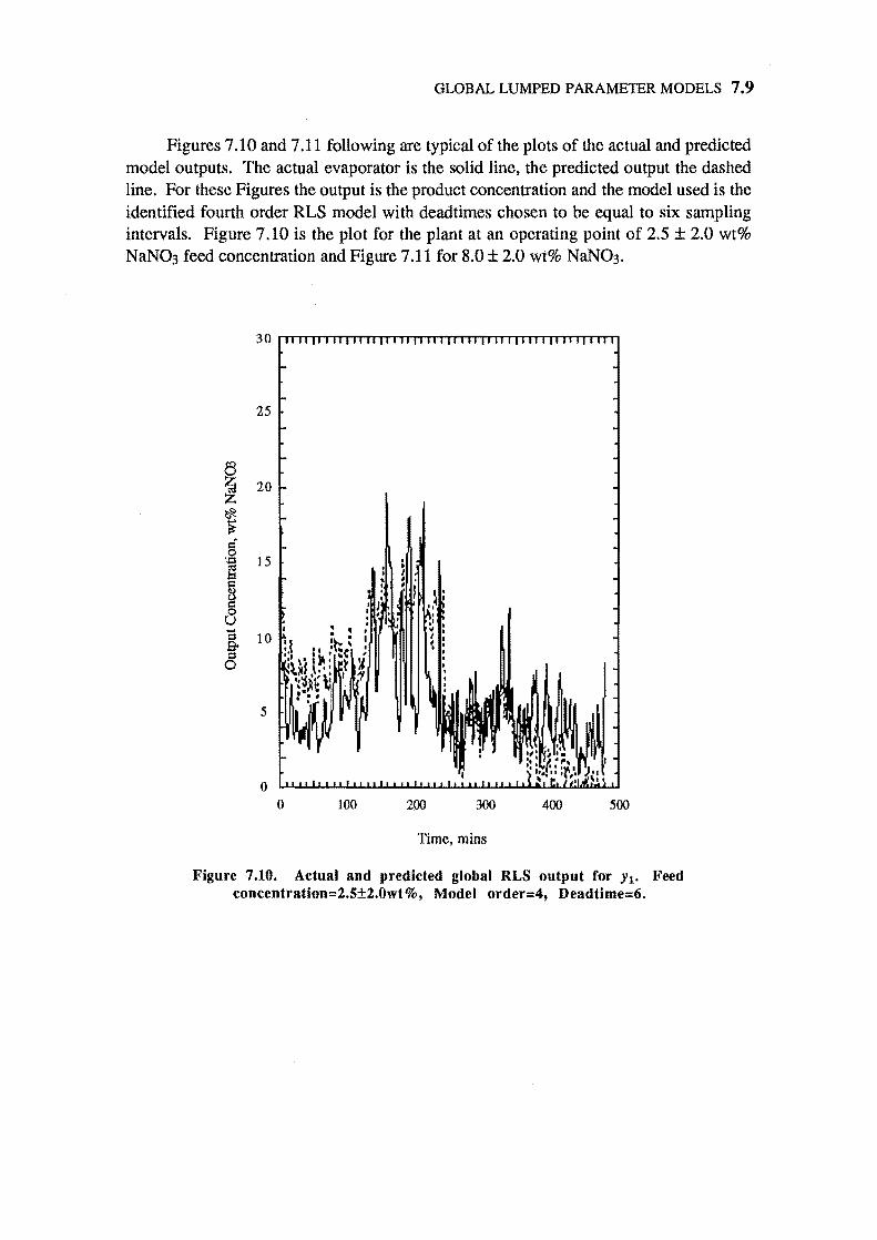
GLOBAL LUMPED PARAMETER MODELS 7.9
Figures 7.10 and 7.11 following are typical of the plots of the actual and predicted model outputs. The actual evaporator is the solid line, the predicted output the dashed line. For these Figures the output is the product concentration and the model used is the identified fourth order RLS model with deadtimes chosen to be equal to six sampling intervals. Figure 7.10 is the plot for the plant at an operating point of 2.5 ± 2.0 wt% NaNOg feed concentration and Figure 7.11 for 8.0 ± 2.0 wt% NaNOg.
25
~ 20 Z ~ .... ~
§ >J:I 15 g · • •
~ I . . I •
• J' ~ . I , • "
u : . .... , . ~ . =' 10 t :t= ~ I
~ t I . t I rwc • ,t t. \I '
0 "\'1" t:4 I~~$.\ •• : I 1 .~~~.,
." I: . : ' 5
o o 100 200 gOO 400 500
Time, mins
Figure 7.10. Actual and predicted global RLS output for Y1' Feed concentration=2.5±2.0wt%, Model order=4, Deadtime=6.
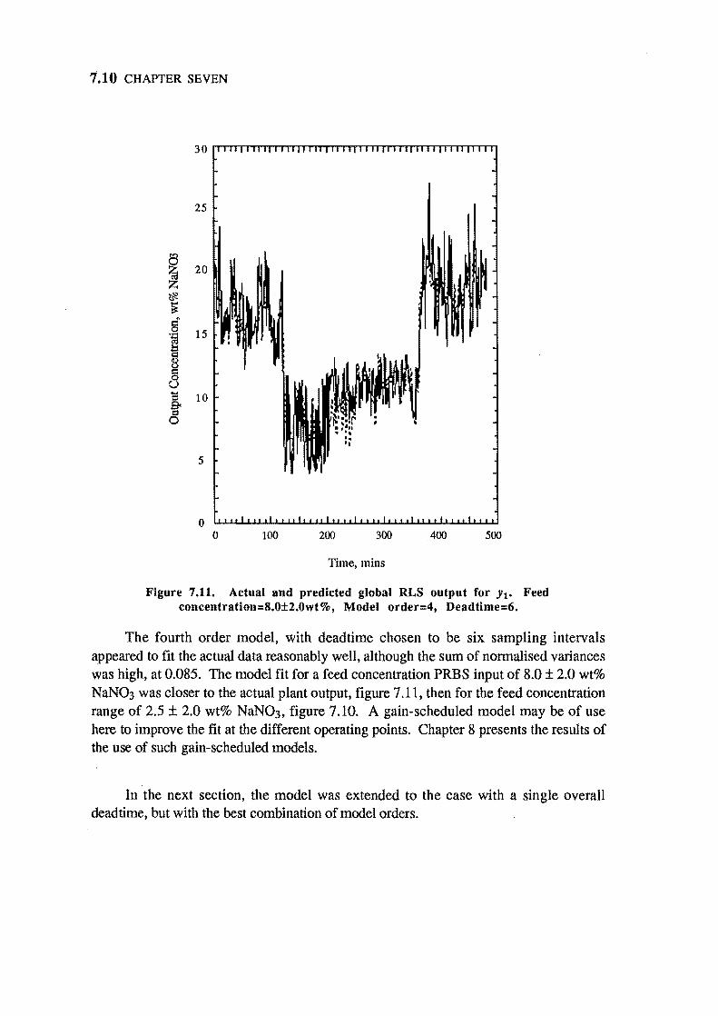
7.10 CHAPTER SEVEN
8
~ 20
~ ~ §
15 'i l:I t:l 8 § u
i 10
0
5
o 100 200 300 400 500
Time, mins
Figure 7.11. Actual and predicted global RLS output for Y1' Feed concentration=8.0±2.0wt%, Model order=4, Deadtime=6.
The fourth order model, with dead time chosen to be six sampling intervals appeared to fit the actual data reasonably well, although the sum of normalised variances was high, at 0.085. The model fit for a feed concentration PRBS input of 8.0 ± 2.0 wt% NaN03 was closer to the actual plant output, figure 7.11, then for the feed concentration range of 2.5 ± 2.0 wt% NaN03, figure 7.10. A gain-scheduled model may be of use here to improve the fit at the different operating points. Chapter 8 presents the results of the use of such gain-scheduled models.
In the next section, the model was extended to the case with a single overall dead time, but with the best combination of model orders.
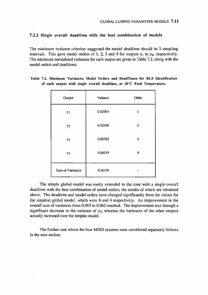
GLOBAL LUMPED PARAMETER MODELS 7.11
7.2.2 Single overall deadtime with the best combination of models
The minimum variance criterion suggested the model dead time should be 3 sampling intervals. This gave model orders of 1, 2, 3 and 4 for outputs Yl to Y4, respectively. The minimum normalised variances for each output are given in Table 7.2, along with the model orders and dead times.
Table 7.2. Minimum Variances, Model Orders and DeadTimes for RLS Identification of each output with siugle overall deadtime, at 20°C Feed Temperature.
Output Variance Otder
Yl 0.02907 1
Y2 0.02486 2
Y3 0.00782 3
Y4 0.00019 4
Sum of Variances 0.06194 -
The simple global model was easily extended to the case with a single overall deadtime with the best combination of model orders, the results of which are tabulated above. The deadtime and model orders have changed significantly from the values for the simplest global model, which were 6 and 4 respectively. An improvement in the overall sum of variances from 0.085 to 0.062 resulted. The improvement was through a significant decrease in the variance of Y2, whereas the variances of the other outputs actually increased over the simpler model.
The further case where the four MISO systems were considered separately follows in the next section.
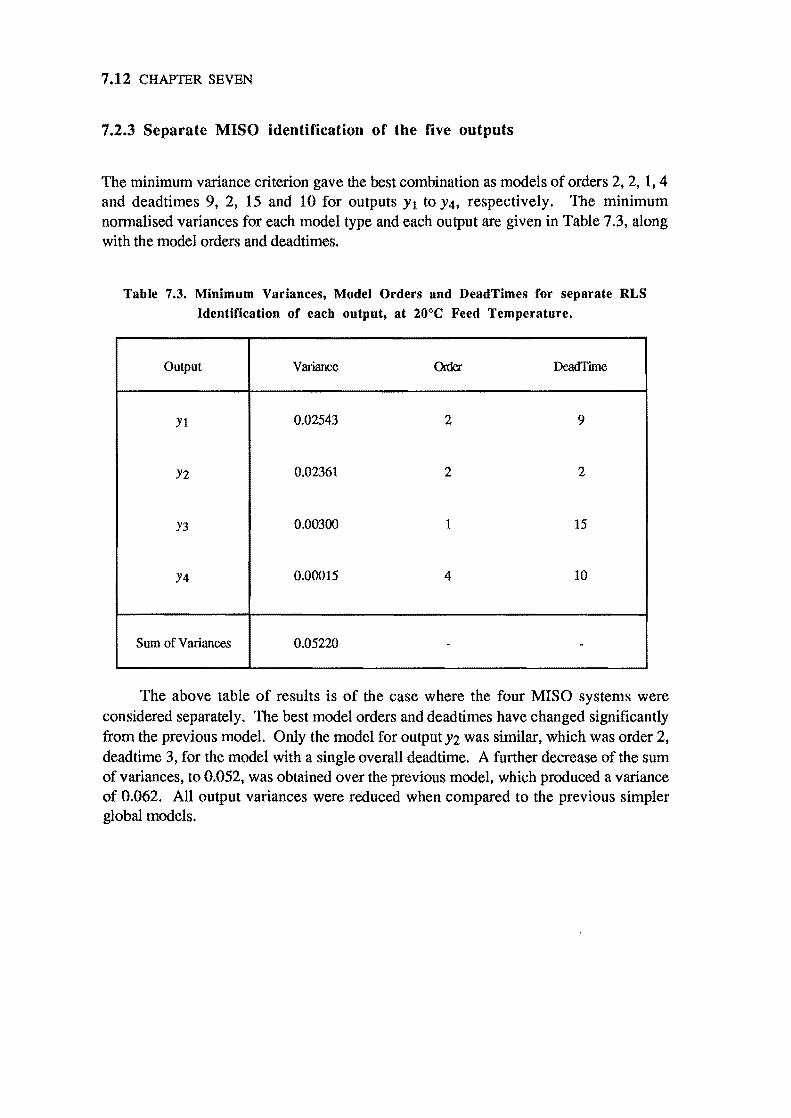
7.12 CHAPTER SEVEN
7.2.3 Separate MISO identification of the five outputs
The minimum variance criterion gave the best combination as models of orders 2, 2, 1, 4 and deadtimes 9, 2, 15 and 10 for outputs Y1 to Y4, respectively. The minimum normalised variances for each model type and each output are given in Table 7.3, along with the model orders and deadtimes.
Table 7.3. Minimum Variances, Model Orders and DeadTimes for separate RLS
Identirication of each output, at 20"C Feed Temperature.
Output Variance Order I>eadTime
Yl 0.02543 2 9
Y2 0.02361 2 2
Y3 0.00300 1 15
Y4 0.00015 4 10
Sum of Variances 0.05220 - -
The above table of results is of the case where the four MISO systems were considered separately. The best model orders and deadtimes have changed significantly from the previous model. Only the model for output Y2 was similar, which was order 2, deadtime 3, for the model with a single overall deadtime. A further decrease of the sum of variances, to 0.052, was obtained over the previous model, which produced a variance of 0.062. All output variances were reduced when compared to the previous simpler global models.
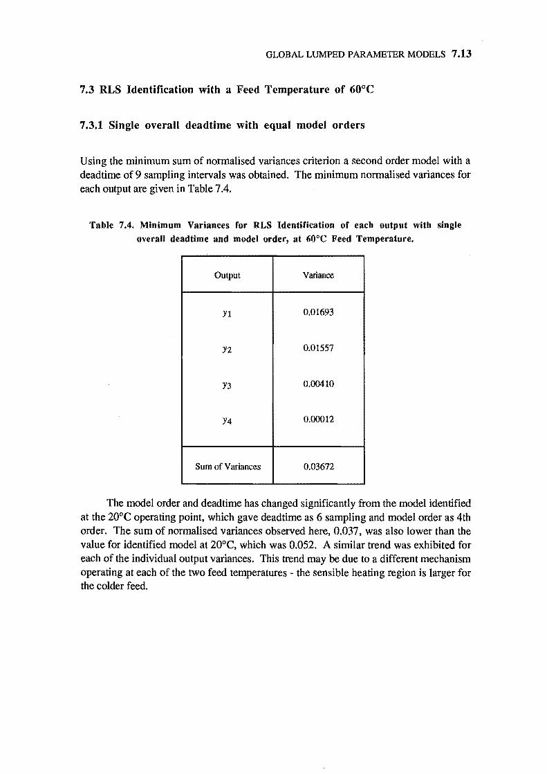
GLOBAL LUMPED PARAMETER MODELS 7.13
7.3 RLS Identification with a Feed Temperature of 60°C
7.3.1 Single overall deadtime with equal model orders
Using the minimum sum of nonnalised variances criterion a second order model with a deadtime of 9 sampling intervals was obtained. The minimum nonnalised variances for each output are given in Table 7.4.
Table 7.4. Minimum Variances for RLS Identification of each output with single
overall dead time and model order, at 60°C Feed Temperature.
Output Variance
Yl 0.01693
Y2 0.01557
Y3 0.00410
Y4 0.00012
Sum of Variances 0.03672
The model order and deadtime has changed significantly from the model identified at the 20°C operating point, which gave deadtime as 6 sampling and model order as 4th order. The sum of nonnalised variances observed here, 0.037, was also lower than the value for identified model at 20°C, which was 0.052. A similar trend was exhibited for each of the individual output variances. This trend may be due to a different mechanism operating at each of the two feed temperatures - the sensible heating region is larger for the colder feed.
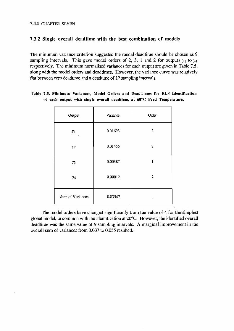
7.14 CHAPTER SEVEN
7.3.2 Single overall deadtime with the best combination of models
The minimum variance criterion suggested the model deadtime should be chosen as 9 sampling intervals. This gave model orders of 2, 3, 1 and 2 for outputs Yl to Y4 respectively. The minimum normalised variances for each output are given in Table 7.5, along with the model orders and deadtimes. However, the variance curve was relatively flat between zero deadtime and a deadtime of 12 sampling intervals.
Table 7.5. Minimum Variances, Model Orders and DeadTimes for RLS Identification
of each output with single overall deadtime, at 60°C Feed Temperature.
Output Variance Order
Yl 0.01693 2
Y2 0.01455 3
Y3 0.00387 1
Y4 0.00012 2
Sum of Variances 0.03547 -
The model orders have changed significantly from the value of 4 for the simplest global model, in common with the identification at 20oe. However, the identified overall deadtime was the same value of 9 sampling intervals. A marginal improvement in the overall sum of variances from 0.037 to 0.035 resulted.
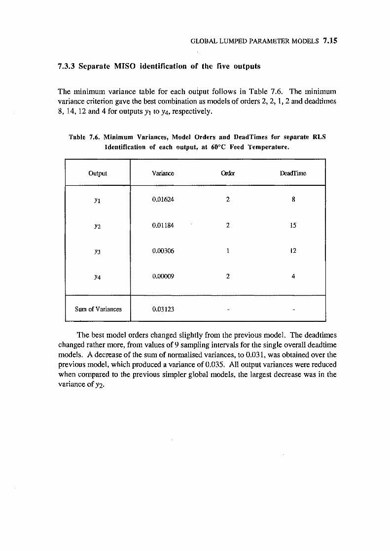
GLOBAL LUMPED PARAMETER MODELS 7.15
7.3.3 Separate MISO identification of the five outputs
The minimum variance table for each output follows in Table 7.6. The minimum variance criterion gave the best combination as models of orders 2, 2, 1, 2 and dead times 8, 14, 12 and 4 for outputs Yt to Y4, respectively.
Table 7.6. Minimum Variances, Model Orders and DeadTimes for separate RLS
Identification of each output, at 60°C Feed Temperature.
Output Variance Qd>r DeadTime
Yl 0.01624 2 8
Y2 0.01184 2 15
Y3 0.00306 1 12
Y4 0.00009 2 4
Sum of Variances 0.03123 " "
The best model orders changed slightly from the previous model. The deadtimes changed rather more, from values of 9 sampling intervals for the single overall dead time models. A decrease of the sum of normalised variances, to 0.031, was obtained over the previous model, which produced a variance of 0.035. All output variances were reduced when compared to the previous simpler global models, the largest decrease was in the variance of Y2.
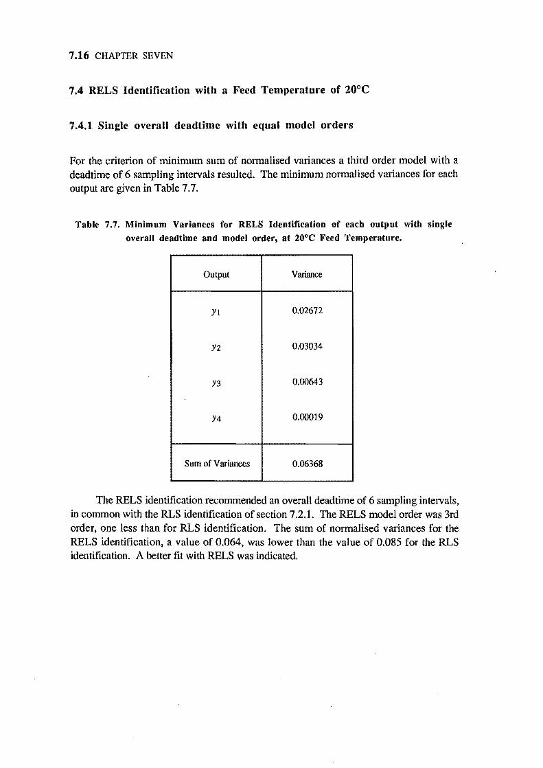
7.16 CHAPTER SEVEN
7.4 RELS Identification with a Feed Temperature of 20°C
7.4.1 Single overall deadtime with equal model orders
For the criterion of minimum sum of normalised variances a third order model with a deadtime of 6 sampling intervals resulted. The minimum normalised variances for each output are given in Table 7.7.
Table 7.7. Minimum Variances for RELS Identification of each output with single overall deadtime and model order,at 20°C Feed Temperature.
Output Variance
Yl 0.02672
Y2 0.03034
Y3 0.00643
Y4 0.00019
Sum of Variances 0.06368
The RELS identification recommended an overall deadtime of 6 sampling intervals, in common with the RLS identification of section 7.2.1. The RELS model order was 3rd order, one less than for RLS identification. The sum of normalised variances for the RELS identification. a value of 0.064. was lower than the value of 0.085 for the RLS identification. A better fit with RELS was indicated.
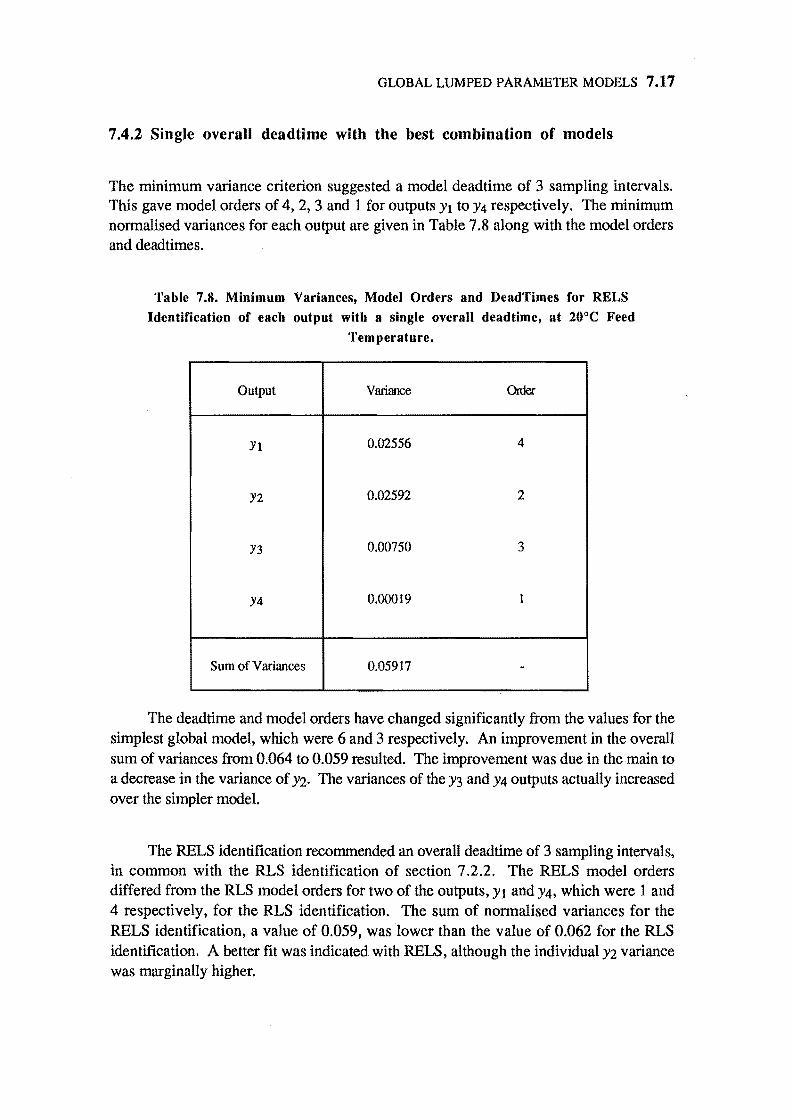
GLOBAL LUMPED PARAMETER MODELS 7.17
7.4.2 Single overall deadtime with the best combination of models
The minimum variance criterion suggested a model deadtime of 3 sampling intervals. This gave model orders of 4, 2, 3 and 1 for outputs Yl to Y4 respectively. The minimum nonnalised variances for each output are given in Table 7.8 along with the model orders and dead times.
Table 7.S. Minimum Variances, Model Orders and DeadTimes for RELS
Identification of each output with a single overall dead time, at 20°C Feed
Temperature.
Output Variance Order
Yl 0.02556 4
Y2 0.02592 2
Y3 0.00750 3
Y4 0.00019 1
Sum of Variances 0.05917 -
The deadtime and model orders have changed significantly from the values for the simplest global model, which were 6 and 3 respectively. An improvement in the overall sum of variances from 0.064 to 0.059 resulted. The improvement was due in the main to a decrease in the variance of Y2. The variances of the Y3 and Y4 outputs actually increased over the simpler model.
The RELS identification recommended an overall dead time of 3 sampling intervals, in common with the RLS identification of section 7.2.2. The RELS model orders differed from the RLS model orders for two of the outputs, Yt and Y4, which were 1 and 4 respectively, for the RLS identification. The sum of nonnalised variances for the RELS identification, a value of 0.059, was lower than the value of 0.062 for the RLS identification. A better fit was indicated with RELS, although the individual Y2 variance was marginally higher.
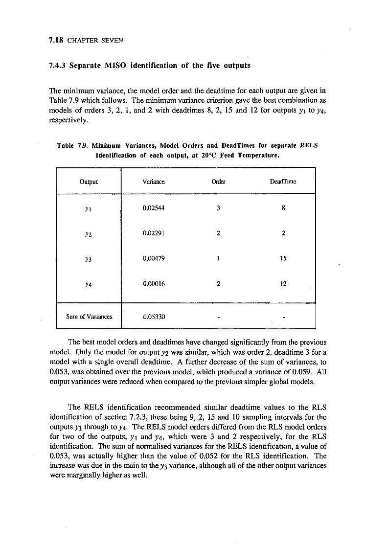
7.18 CHAPTER SEVEN
7.4.3 Separate MISO identification of the five outputs
The minimum variance, the model order and the dead time for each output are given in Table 7.9 which follows. The minimum variance criterion gave the best combination as models of orders 3, 2, I, and 2 with deadtimes 8, 2, 15 and 12 for outputs Yl to Y4, respectively.
Table 7.9. Minimum Variances, Model Orders and DeadTimes for separate RELS Identification of each output, at 20°C Feed Temperature.
Output Variance 0nIer DeadTirne
Yl 0.02544 3 8
Y2 0.02291 2 2
Y3 0.00479 1 15
Y4 0.00016 2 12
Sum of Variances 0.05330 - .
The best model orders and dead times have changed significantly from the previous model. Only the model for output Y2 was similar, which was order 2, deadtime 3 for a model with a single overall deadtime. A further decrease of the sum of variances, to 0.053, was obtained over the previous model, which produced a variance of 0.059. All output variances were reduced when compared to the previous simpler global models.
The RELS identification recommended similar deadtime values to the RLS identification of section 7.2.3, these being 9, 2, 15 and 10 sampling intervals for the outputs Yl through to Y4. The RELS model orders differed from the RLS model orders for two of the outputs, Yl and Y4, which were 3 and 2 respectively, for the RLS identification. The sum of normalised variances for the RELS identification, a value of 0.053, was actually higher than the value of 0.052 for the RLS identification. The increase was due in the main to the Y3 variance, although all of the other output variances were marginally higher as well.
GLOBAL LUMPED PARAMETER MODELS 7.19
7.5 RELS Identification with a Feed Temperature of 60°C
7.5.1 Single overall deadtime with equal model orders
The best model available according to the minimum sum of nonnalised variances criterion was a fourth order model with a deadtime of 9 sampling intervals. The minimum nonnalised variances for each each output are given in Table 7.10.
Table 7.10. Minimum Variances for RELS Identification of each output with single
overall deadtime and model order, at 60°C Feed Temperature.
Output Variance
Yl 0.01945
Y2 0.01493
Y3 0.00384
Y4 0.00038
Sum of Variances 0.03860
The model order and deadtime has changed from the model identified at the 20°C operating point, which gave deadtime as 6 sampling and the model order as 3rd order. The sum of nonnalised variances observed here, 0.039, was also lower than the value for identified model at 20°C, which was 0.064. A similar trend was exhibited for each of the individual output variances, with the exception of Y4.
The RELS identification recommended an overall deadtime of 9 sampling intervals, in common with the RLS identification of section 7.3.1. The RLS model order was 2nd order, two less than for RELS identification. The sum of normalised variances for the RELS identification, a value of 0.039, was higher than the value of 0.037 for the RLS identification, indicating a better fit was obtained from RLS identification. The variances of outputs Yl and Y4 were responsible for the increase in the overall variance.
7.20 CHAPTER SEVEN
7.5.2 Single overall deadtime with the best combination of models
The minimum variance criterion gave the deadtime as 11 sampling intervals. Models resulted of order I, 2, 1 and 2 for outputs Y1 to Y4 respectively. The minimum normalised variances for each output are given in Table 7.11. along with the model orders and deadtimes.
Table 7.11. Minimum Variances, Model Orders and DeadTimes for RELS IdentiFication of each output with a single overall deadtime, at 60°C Feed
Temperature.
Output Variance Order
Y1 0.01785 1 ,
Y2 0.01270 2
Y3 0.00354 1
Y4 0.00019 2
Sum of Variances 0.03428 -
The model orders have changed significantly from the value of 4 for the simplest global model. The identified overall deadtime changed from a value of 9 to 11 sampling intervals. A marginal improvement in the overall sum of variances from 0.039 to 0.034 resulted. The improvement was through a decrease in the variances of both Yl and Y2. over the simpler model. The variances of the other outputs decreased by smaller amounts.
The RELS model orders and deadtime differed from those of the RLS models. The orders for two of the outputs. Yl and Y2. changed from 2 and 3 for the RLS identification. The RLS identification of section 7.3.2 recommended a different overall deadtime of 9 sampling intervals. The sum of normalised variances for the RELS identification. a value of 0.034. was lower than the value of 0.035 for the RLS identification •. A better fit with RELS was indicated. although the individual Yl andY4 variances were higher.
GLOBAL LUMPED PARAMETER MODELS 7.21
7.5.3 Separate MISO identification of the five outputs
The minimum variances for each output are presented in Table 7.12, along with the best model orders and dead times. The minimum variance criterion gave the best combination as models of orders 1, I, 3 and 4 with dead times 7, 15, 12 and 5 for outputs Yl to Y4, respectively.
Table 7.12. Minimum Variances, Model Orders and DeadTimes for separate RELS
Identification of each output, at 60°C Feed Temperature.
Output Variance CK<:b: DeadTime
Yl 0.01681 1 7
Y2 0.01181 1 15
Y3 0.00332 3 12
Y4 0.00011 4 5
Sum of Variances 0.03205 - -
The best model orders changed from the previous model. The deadtimes changed rather more, from values of 11 sampling intervals for the single overall deadtime models. A decrease of the sum of normalised variances, to 0.032, was obtained over the previous model, which produced a variance of 0.034. All output variances were reduced when compared to the previous simpler global models, the largest decrease was in the variance of Yl.
The RELS identification recommended similar dead time values to the RLS identification of section 7.3.3, these being 8, 15, 12 and 5 sampling intervals for the outputs Yl through to Y4. The RELS model orders differed from the RLS model orders for all of the outputs, Yl to Y4, which were 2, 2, 1 and 2 respectively, for the RLS identification. The sum of normalised variances for the RELS identification, a value of 0.032, was actually higher than the value of 0.031 for the RLS identification. All of the other output variances were higher, with the exception of the Y2 variance value.
7.22 CHAPTER SEVEN
7.6 Conclusions
Separate MISO identification gave the best results based on the sum of normalised variances criterion, of the three types of models proposed - single overall deadtime with equal model orders, single overall dead time with differing model orders and separate identification of each output.
There was little or no improvement to be gained from RELS identification over RLS identification. In fact, separate MISO identification showed a marginal increase in the sum of normalised variances in some cases. This might be ascribed to the global model being inadequate across the entire operating range. A gain scheduled model may be more appropriate to describe the plant at different operating points.
A difference between the identified models at the two feed temperature setpoints considered was apparent. Both the model deadtimes and orders change.
The reason may be due to a different mechanism operating at each temperature. At 20 "c the feed enters the evaporator tube considerably below the boiling point of the liquid in the tube - at least 40 "c below the boiling point at the vacuum pressure used. This means there is a large sensible heating region where the liquid feed is heated up to the boiling point. At a feed temperature of 60 "c the feed enters the evaporator tube at just below the boiling point, so the sensible heating region is much shorter. This will change the time constants and deadtimes of the process. If the evaporator tube is regarded as a small tank filled with liquid, the volume and height of this tank has effectively changed. This change in the tank dynamics is reflected by a change in the identified parameters.
The apparent difference between the identified models at the two feed temperature setpoints is also a possible consequence of the distributed nature of the system. The change of order may be seen as a distributed effect. As noted in section 3.2, increasing model order can account for distributed or deadtime processes in some situations. To give a reverse example of this, a fifth order process can be modelled by a first order plus deadtime model in may cases.
Overall, it seems that the recursive lumped parameter methods gave poor results for the identification of the simple global models. The gain scheduled and distributed approaches may yield better results. These methods are examined in the following two chapters.
GLOBAL LUMPED PARAMETER MODELS 7.23
ABBREVIATIONS
MISO
RLS
RELS
Multi-Input, Single-Output
Recursive Least Squares
Recursive Extended Least Squares
SYMBOLS
d Model dead time in sampling intervals
Kmi Model gain with respect to input i
Lm Model dead time across all inputs
T mi Model time constant with respect to input i
u 1 S team temperature in the steam jacket on the evaporator tube
u2 Feed flowrate to the evaporator
u3 Temperature of the evaporator feed
u4 Concentration of the evaporator feed
Y 1 Concentration of the product concentrate,
Y2 Exit flowrate of the product concentrate
Y3 Temperature of the product concentrate
Y 4 Concentration of the product condensate

CHAPTER
EIGHT
GAIN SCHEDULED LUMPED MODELS
In which the identification procedures outlined in chapter 4 are applied to gainwscheduled models of the climbing film evaporator. The resulting identified models are presented and discussed.
8.1 A GAIN SCHEDULED MODEL OF THE EVAPORATOR
In this chapter, the results are presented from the identification of the climbing film evaporator as a series of simple linear models at each individual operating point.
This approach has been termed gain scheduling (Astrom and Wittenmark, 1984), and is a method used for systems whose parameters change with operating conditions. The use of this technique in control may be considered as a form of adaptive control, where the parameters of the controller are altered according to the variation in process parameters with a known change in the plant operating point. Originally this approach was used only to account for change in process gains, hence the name gain scheduling.
The major drawback of gain scheduling is that it is an open-loop compensation for changes in process parameters. The gain schedule must be designed before applying the controller to the process. There is no feedback to compensate for incorrect schedules.
The advantage of gain scheduling is that the regulator parameters can be changed quickly and easily in response to process parameter variations.
8.1
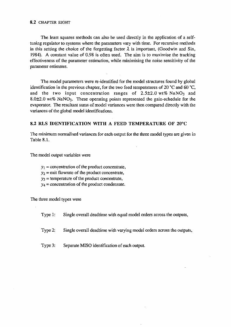
8.2 CHAPTER EIGHT
The least squares methods can also be used directly in the application of a selftuning regulator to systems where the parameters vary with time. For recursive methods in this setting the choice of the forgetting factor A., is important, (Goodwin and Sin, 1984). A constant value of 0.98 is often used. The aim is to maximise the tracking effectiveness of the parameter estimation, while minimising the noise sensitivity of the parameter estimates.
The model parameters were re-identified for the model structures found by global identification in the previous chapter, for the two feed temperatures of 20 ·C and 60 ·C, and the two input concentration ranges of 2.5±2.0 wt% NaN03 and 8.0±2.0 wt% NaN03. These operating points represented the gain-schedule for the evaporator. The resultant sums of model variances were then compared directly with the variances of the global model identifications.
8.2 RLS IDENTIFICATION WITH A FEED TEMPERATURE OF 20°C
The minimum normalised variances for each output for the three model types are given in Table 8.1.
The model output variables were
Yt = conyentration of the product concentrate, Y2 = exit flowrate of the product concentrate, Y3 = temperature of the product concentrate, Y4 = concentration of the product condensate.
The three model types were
Type 1: Single overall dead time with equal model orders across the outputs,
Type 2: Single overall deadtime with varying model orders across the outputs,
Type 3: Separate MISO identification of each output.
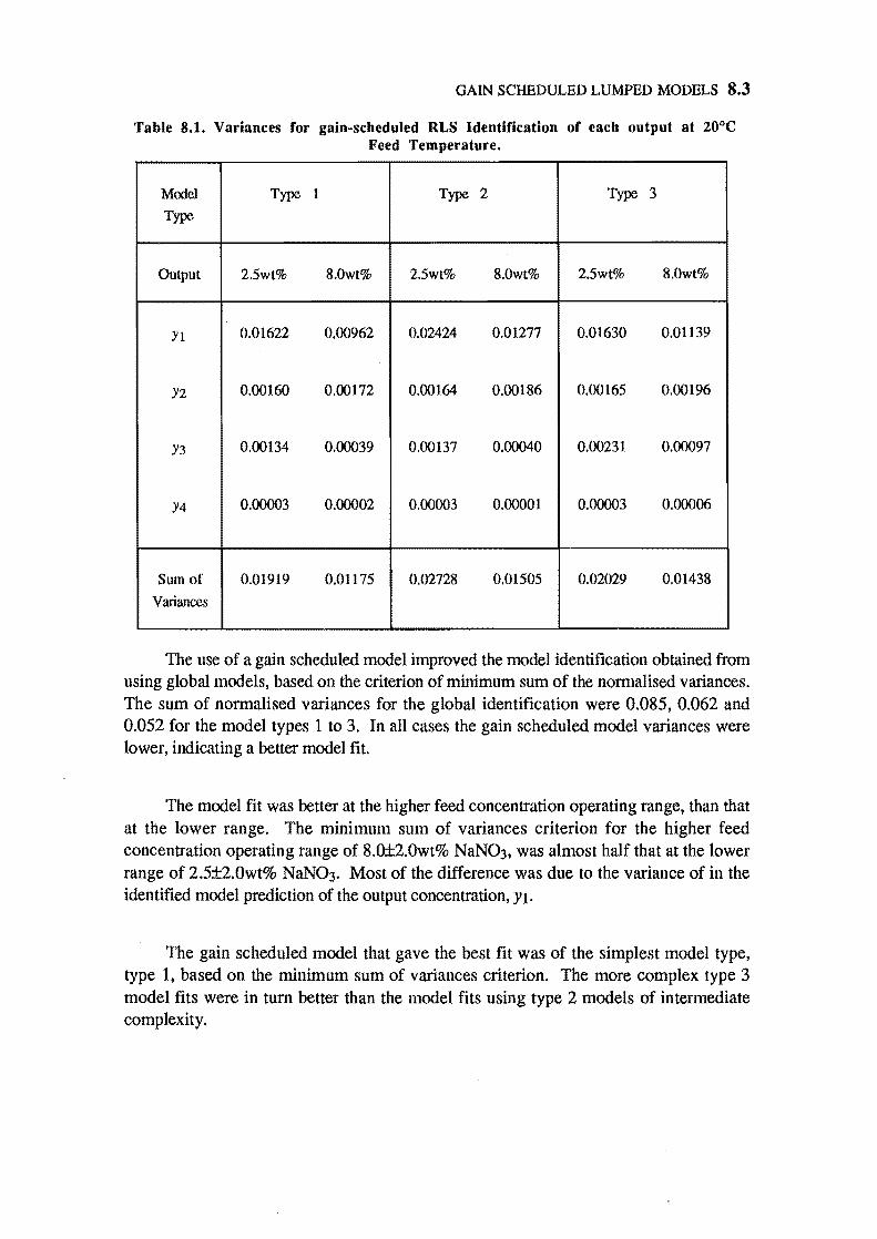
GAIN SCHEDULED LUMPED MODELS 8.3
Table 8.1. Variances for gain-scheduled RLS Identification of each output at 20°C Feed Temperature.
Model Type 1 Type 2 Type 3
Type
Output 2.5wt% 8.0wt% 2.5wt% 8.0wt% 2.5wt% 8.0wt%
Yl 0.01622 0.00962 0.02424 0.01277 0.01630 0.01139
Y2 0.00160 0.00172 0.00164 0.00186 0.00165 0.00196
Y3 0.00134 0.00039 0.00137 0.00040 0.00231 0.00097
Y4 0.00003 0.00002 0.00003 0.00001 0.00003 0.00006
Sum of 0.01919 0.01175 0.02728 0.01505 0.02029 0.01438
Variances
The use of a gain scheduled model improved the model identification obtained from using global models, based on the criterion of minimum sum of the nonnalised variances. The sum of nonnalised variances for the global identification were 0.085, 0.062 and 0.052 for the model types 1 to 3. In all cases the gain scheduled model variances were lower, indicating a better model fit.
The model fit was better at the higher feed concentration operating range, than that at the lower range. The minimum sum of variances criterion for the higher feed concentration operating range of 8.o±2.0wt% NaN03, was almost half that at the lower range of 2.5±2.0wt% NaN03. Most of the difference was due to the variance of in the identified model prediction of the output concentration, Y1.
The gain scheduled model that gave the best fit was of the simplest model type, type 1, based on the minimum sum of variances criterion. The more complex type 3 model fits were in turn better than the model fits using type 2 models of intennediate complexity.
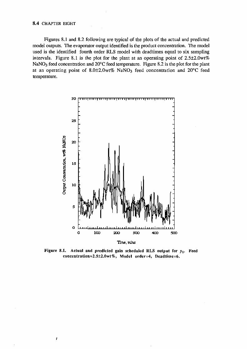
8.4 CHAPTER EIGHT
Figures 8.1 and 8.2 following are typical of the plots of the actual and predicted model outputs. The evaporator output identified is the product concentration. The model used is the identified fourth order RLS model with deadtimes equal to six sampling intervals. Figure 8.1 is the plot for the plant at an operating point of 2.5±2.0wt% NaN03 feed concentration and 200 e feed temperature. Figure 8.2 is the plot for the plant at an operating point of 8.0±2.0wt% NaN03 feed concentration and 200 e feed temperature.
15
10
s
o o
TIme,mins
Figure 8.1. Actual and predicted gain scheduled RLS output for Yl' Feed concentration=2.5±2.0wt%, Model order=4, Deadtime=6.
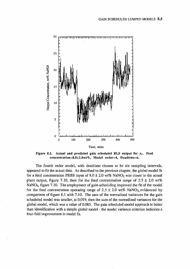
GAIN SCHEDULED LUMPED MODELS 8.5
a ~ 20
~ .... ~ d' 0 '0
~ 15
~ 8 d ~
10
0
5
o 100 200 300 400 500
Time, mins
Figure 8.2. Actual and predicted gain scheduled RLS output for Yl' Feed concentration=8.0±2.0wt%, Model order=4, Deadtime=6.
The fourth order model, with deadtime chosen to be six sampling intervals, appeared to fit the actual data. As described in the previous chapter, the global model fit for a feed concentration PRBS input of 8.0 ± 2.0 wt% NaN03 was closer to the actual plant output, figure 7.10, then for the feed concentration range of 2.5 ± 2.0 wt% NaN03, figure 7.10. The employment of gain-scheduling improved the fit of the model for the feed concentration operating range of 2.5 ± 2.0 wt% NaN03, evidenced by comparison of figure 8.1 with 7.10. The sum of the normalised variances for the gain scheduled model was smaller, at 0.019, then the sum of the normalised variances for the global model, which was a value of 0.085. The gain scheduled model approach is better than identification with a simple global model - the model variance criterion indicates a four-fold improvement in model fit.
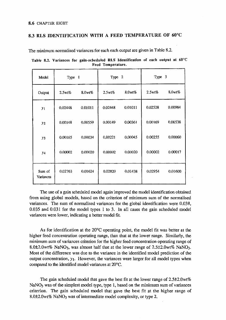
8.6 CHAPTER EIGHT
8.3 RLS IDENTIFICATION WITH A FEED TEMPERATURE OF 60°C
The minimum nonnalised variances for each each output are given in Table 8.2.
Table 8.2. Variances for gain-scheduled RLS Identification of each output at 60"C Feed Temperature.
Model Type 1 Type 2 Type 3
Output 2.5wt% 8.0wt% 2.5wt% 8.0wt% 2.5wt% 8.0wt%
Yl 0.02448 0.01011 0.02448 0.01011 0.02528 0.00984
Y2 0.00148 0.00559 0.00149 0.00361 0.00169 0.00538
Y3 0.00165 0.00034 0.00221 0.00045 0.00255 0.00060
Y4 0.00002 0.00020 0.00002 0.00020 0.00002 0.00017
Sum of 0.02763 O.ot624 0.02820 0.01438 0.02954 0.01600
Variances
The use of a gain scheduled model again improved the model identification obtained from using global models, based on the criterion of minimum sum of the nonnalised variances. The sum of nonnalised variances for the global identification were 0.038, 0.035 and 0.031 for the model types 1 to 3. In all cases the gain scheduled model variances were lower, indicating a better model fit.
As for identification at the 20°C operating point, the model fit was better at the higher feed concentration operating range, than that at the lower range. Similarly, the minimum sum of variances criterion for the higher feed concentration operating range of 8.0±2.0wt% NaN03, was almost half that at the lower range of 2.5±2.0wt% NaN03. Most of the difference was due to the variance in the identified model prediction of the output concentration, Yl. However, the variances were larger for all model types when compared to the identified model variances at 20°C.
The gain scheduled model that gave the best fit at the lower range of 2.5±2.0wt% NaNDJ was of the simplest model type, type I, based on the minimum sum of variances criterion. The gain scheduled model that gave the best fit at the higher range of 8.0±2.0wt% NaN03 was of intennediate model complexity, or type 2.
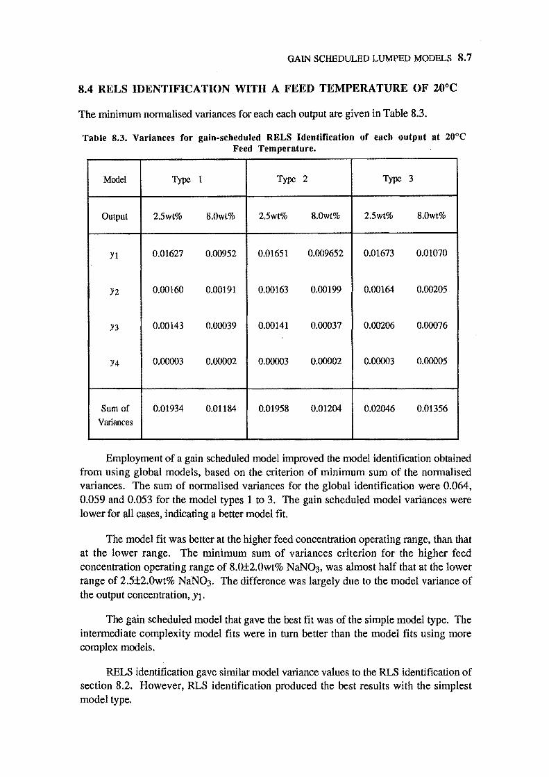
GAIN SCHEDULED LUMPED MODELS 8.7
8.4 RELS IDENTIFICATION WITH A FEED TEMPERATURE OF 20°C
The minimum nonnalised variances for each each output are given in Table 8.3.
Table 8.3. Variances for gain-scheduled RELS Identification of each output at 20°C Feed Temperature.
Model Type 1 Type 2 Type 3
Output 2.5wt% 8.0wt% 2.5wt% 8.0wt% 2.5wt% 8.0wt%
Yl 0.01627 0.00952 0.01651 0.009652 0.01673 0.01070
Y2 0.00160 0.00191 0.00163 0.00199 0.00164 0.00205
Y3 0.00143 0.00039 0.00141 0.00037 0.00206 0.00076
Y4 0.00003 0.00002 0.00003 0.00002 0.00003 0.00005
Sum of 0.01934 0.01184 0.01958 0.01204 0.02046 0.01356
Variances
Employment of a gain scheduled model improved the model identification obtained from using global models, based on the criterion of minimum sum of the nonnalised variances. The sum of nonnalised variances for the global identification were 0.064, 0.059 and 0.053 for the model types 1 to 3. The gain scheduled model variances were lower for all cases, indicating a better model fit.
The model fit was better at the higher feed concentration operating range, than that at the lower range. The minimum sum of variances criterion for the higher feed concentration operating range of 8.0±2.0wt% NaN03, was almost half that at the lower range of 2.5±2.0wt% NaN03. The difference was largely due to the model variance of the output concentration, Yl.
The gain scheduled model that gave the best fit was of the simple model type. The intennediate complexity model fits were in turn better than the model fits using more complex models.
RELS identification gave similar model variance values to the RLS identification of section 8.2. However, RLS identification produced the best results with the simplest model type.
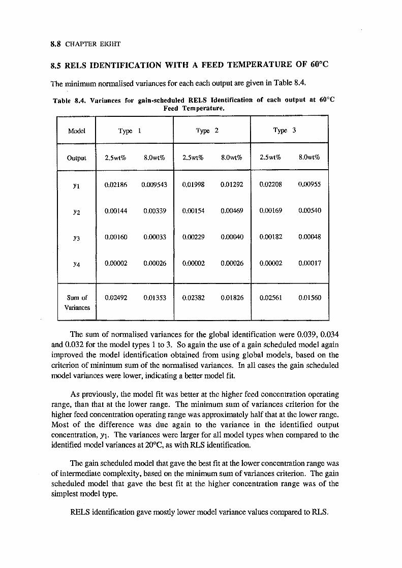
8.8 CHAPTER EIGHT
8.5 RELS IDENTIFICATION WITH A FEED TEMPERATURE OF 60°C
The minimum nonnalised variances for each each output are given in Table 8.4.
Table 8.4. Variances for gain-scheduled RELS Identification of each output at 60°C Feed Temperature.
Model Type 1 Type 2 Type 3
Output 2.5wt% 8.0wt% 2.5wt% 8.0wt% 2.5wt% 8.0wt%
Y1 0.02186 0.009543 0.01998 0.01292 0.02208 0.00955
Y2 0.00144 0.00339 0.00154 0.00469 0.00169 0.00540
Y3 0.00160 0.00033 0.00229 0.00040 0.00182 0.00048
Y4 0.00002 0.00026 0.00002 0.00026 0.00002 0.00017
Sum of 0.02492 0.01353 0.02382 0.01826 0.02561 0.01560
Variances
The sum of nonnalised variances for the global identification were 0.039, 0.034 and 0.032 for the model types 1 to 3. So again the use of a gain scheduled model again improved the model identification obtained from using global models, based on the criterion of minimum sum of the nonnalised variances. In all cases the gain scheduled model variances were lower, indicating a better model fit.
As previously, the model fit was better at the higher feed concentration operating range, than that at the lower range. The minimum sum of variances criterion for the higher feed concentration operating range was approximately half that at the lower range. Most of the difference was due again to the variance in the identified output concentration, Y1. The variances were larger for all model types when compared to the identified model variances at 20°C, as with RLS identification.
The gain scheduled model that gave the best fit at the lower concentration range was of intermediate complexity, based on the minimum sum of variances criterion. The gain scheduled model that gave the best fit at the higher concentration range was of the simplest model type.
RELS identification gave mostly lower model variance values compared to RLS.
GAIN SCHEDULED LUMPED MODELS 8.9
8.6 CONCLUSIONS
Based on the sum of normalised variances criterion, the gain-scheduled identification approach gave better results than the global model identification. A comparison with the identified global models indicated the variances had been approximately halved. This can be seen as a consequence of the better prediction at the two different feed concentration operating ranges.
Of the three types of models, separate MISO identification did not necessarily give the best results. The simplest model type identified was a model with a single overall deadtime and order. RLS identification with the simplest model type was superior for many operating ranges.
There was little improvement to be gained from RELS identification over RLS identification. In some instances slight increases in the sum of normalised variances were observed for RELS identification. It was hoped that a gain scheduled model would have been able to solve this problem. It appears instead that this phenomenon may also be due to the distributed nature of the system - lumped parameter treatments may be simply inadequate to describe this example of the evaporator behaviour. The compensation of noise-process estimation which is an advantage of using RELS was insufficient to overcome this problem as RELS is only a lumped parameter identification method.
Overall, the recursive lumped parameter methods gave good results for the identification of gain scheduled models. The obseIved discrepancies may be due to the distributed nature of the system - distributed parameter identification of evaporator models is investigated in the next chapter.
ABBREVIATIONS
MISO Multi-Input. Single-Output
RLS Recursive Least Squares
RELS Recursive Extended Least Squares
SYMBOLS
d Model deadtime in sampling intervals
Ul Steam temperature in the steam jacket on the evaporator tube
U2 Feed flowrate to the evaporator
U3 Tempemture of the evapomtor feed
8.10 CHAPTER EIGHT
U4 ConcenlIation of the evaporator feed
Y 1 ConcenlIation of the product concentrate,
Y2 Exit flowrate of the product concentrate
Y3 Temperature of the product concentrate
Y 4 ConcenlIation of the product condensate
It Forgetting factor
REFERENCES
A.str6m,K.J. and Wittenmark,B., "Computer Controlled Systems: Theory and Design",
Prentice-Hall International. pp351-352 (1984).
Goodwin, G.C. and Sin, K.S •• "Adaptive filtering prediction and control". Prentice-Hall (1984).
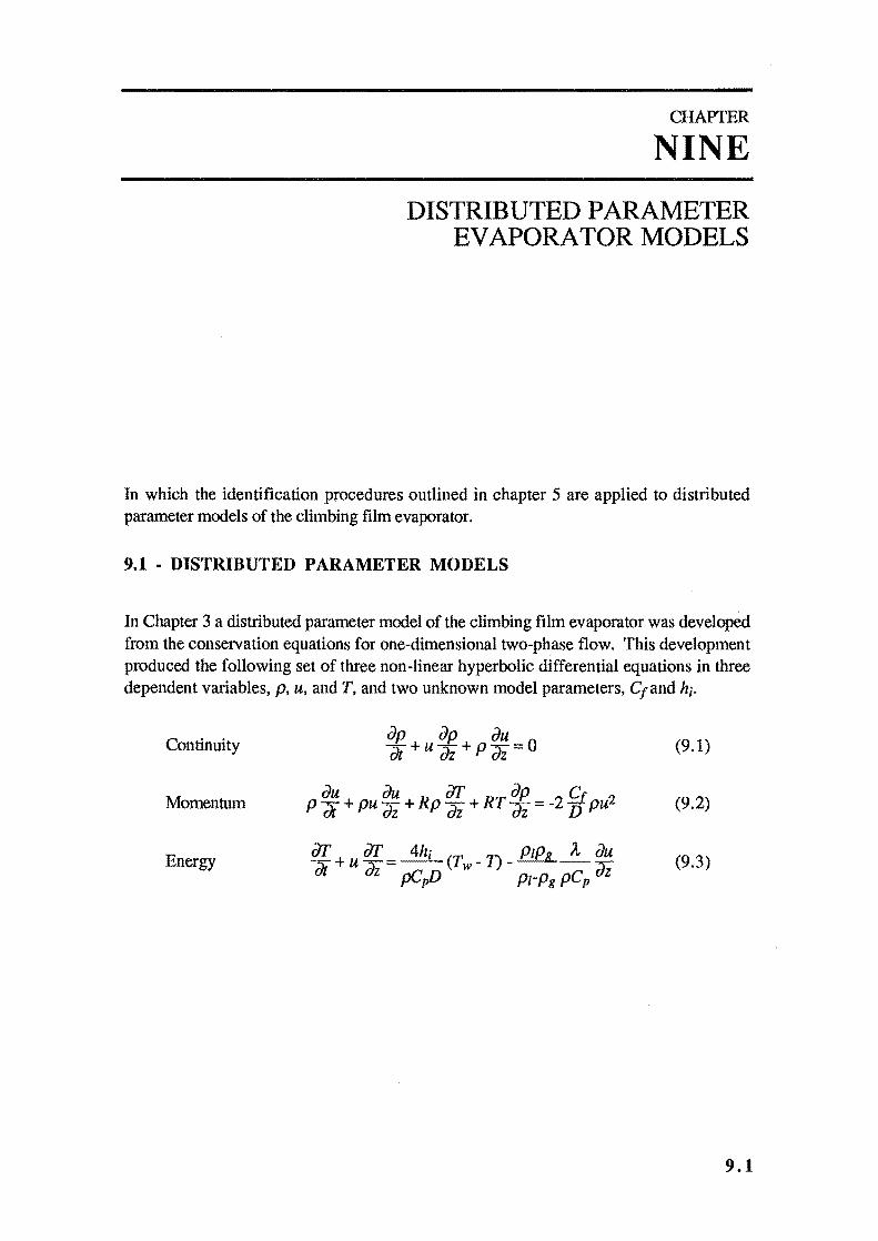
CHAPTER
NINE
DISTRIBUTED PARAMETER EV APORATOR MODELS
In which the identification procedures outlined in chapter 5 are applied to distributed parameter models of the climbing film evaporator.
9.1 . DISTRIBUTED PARAMETER MODELS
In Chapter 3 a distributed parameter model of the climbing film evaporator was developed from the conservation equations for one-dimensional two-phase flow. This development produced the following set of three non-linear hyperbolic differential equations in three dependent variables, p, u, and T, and two unknown model parameters, Cf and hi.
Continuity iJp iJp iJu -+u-+ P"""L=O at iJz flZ
(9.1)
Momentum (9.2)
Energy (9.3)
9.1
9.2 CHAPTER NINE
where Cr= homogeneous friction factor, Cp = homogeneous mixture heat capacity, D = evaporator tube diameter, hi = internal heat transfer coefficient from the evaporator steam jacket to the fluid, t = time, T = homogeneous mixture temperature, T w = evaporator steam jacket temperature, u = homogeneous mixture velocity, z = distance up the evaporator tube, A. = latent heat of vaporisation P = homogeneous mixture density, Pg = vapour density, PI = liquid density.
The following optimisation scheme was considered to identify the parameters of this non-linear model directly.
Firstly, an initial estimate of the parameters of the model would be required. The response of the model calculated from the method of characteristics scheme, section 3.3, would then be compared with the actual observed behaviour of the climbing film evaporator plant. Then the difference between the model outputs and the plant outputs may be used in some form of minimisation function. The most obvious choice would be the output least square error (OLSE) criterion. The initial estimate of the models would then be refined in some fashion using the OLSE criterion, and the model response recalculated. The preceding two steps would then be repeated until the value of the OLSE criterion was acceptably small.
The difficulty with this scheme is updating the model parameters at each iteration. The model equations are highly non-linear and hyperbolic with characteristics. The consequence of these factors is that the gradient of the OLSE criterion is extremely difficult to obtain analytically.
The multiplicative non-linearities of the model equations must be removed to enable use of the method of characteristics, as applied by Carpenter et al. (1971). This process yields linear distributed parameter models of the climbing film evaporator to be identified.
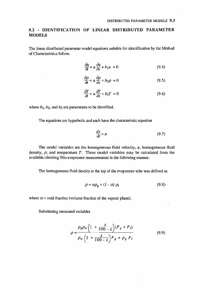
DISTRIBUTED PARAMETER MODELS 9.3
9.2 - IDENTIFICATION OF LINEAR DISTRIBUTED PARAMETER MODELS
The linear distributed parameter model equations suitable for identification by the Method of Characteristics follow.
(9.4)
a: + u fJ: + b2P = 0 (9.5)
(9.6)
where bl. b2, and b3 are parameters to be identified.
The equations are hyperbolic and each have the characteristic equation
dz dt = U (9.7)
The model variables are the homogeneous fluid velocity, u, homogeneous fluid density, p, and temperature T. These model variables may be calculated from the available climbing film evaporator measurements in the following manner.
The homogeneous fluid density at the top of the evaporator tube was defined as
where a = void fraction (volume fraction of the vapour phase).
Substituting measured variables
P = PgPw (1 + lOt _ x ) (F g + F ,)
Pw (1 + lOt _ x ) F g + P g F 1
(9.8)
(9.9)
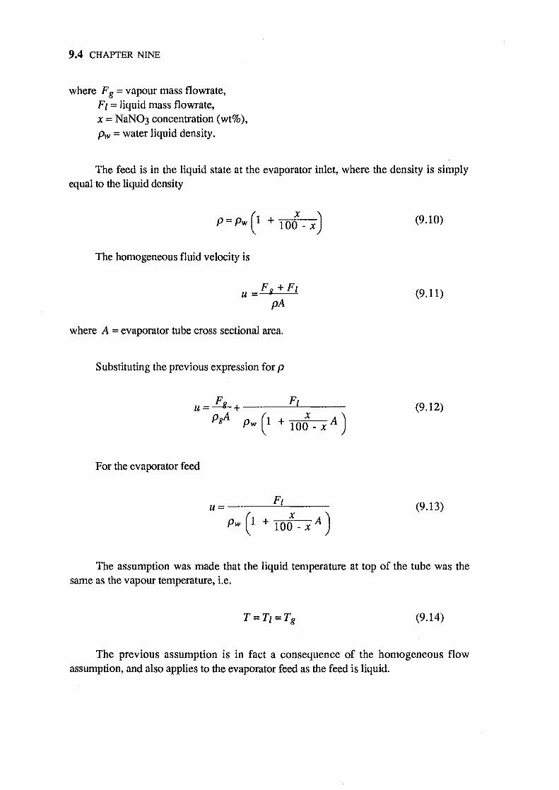
9.4 CHAPTER NINE
where F g = vapour mass flowrate, F/ = liquid mass flowrate, x = NaN03 concentration (wt%), Pw = water liquid density.
The feed is in the liquid state at the evaporator inlet, where the density is simply equal to the liquid density
The homogeneous fluid velocity is
U = F Il + Fl pA
where A = evaporator tube cross sectional area.
Substituting the previous expression for p
For the evaporator feed
(9.10)
(9.11)
(9.12)
(9.13)
The assumption was made that the liquid temperature at top of the tube was the same as the vapour temperature, i.e.
T=T/ =Tg (9.14)
The previous assumption is in fact a consequence of the homogeneous flow assumption, and also applies to the evaporator feed as the feed is liquid.
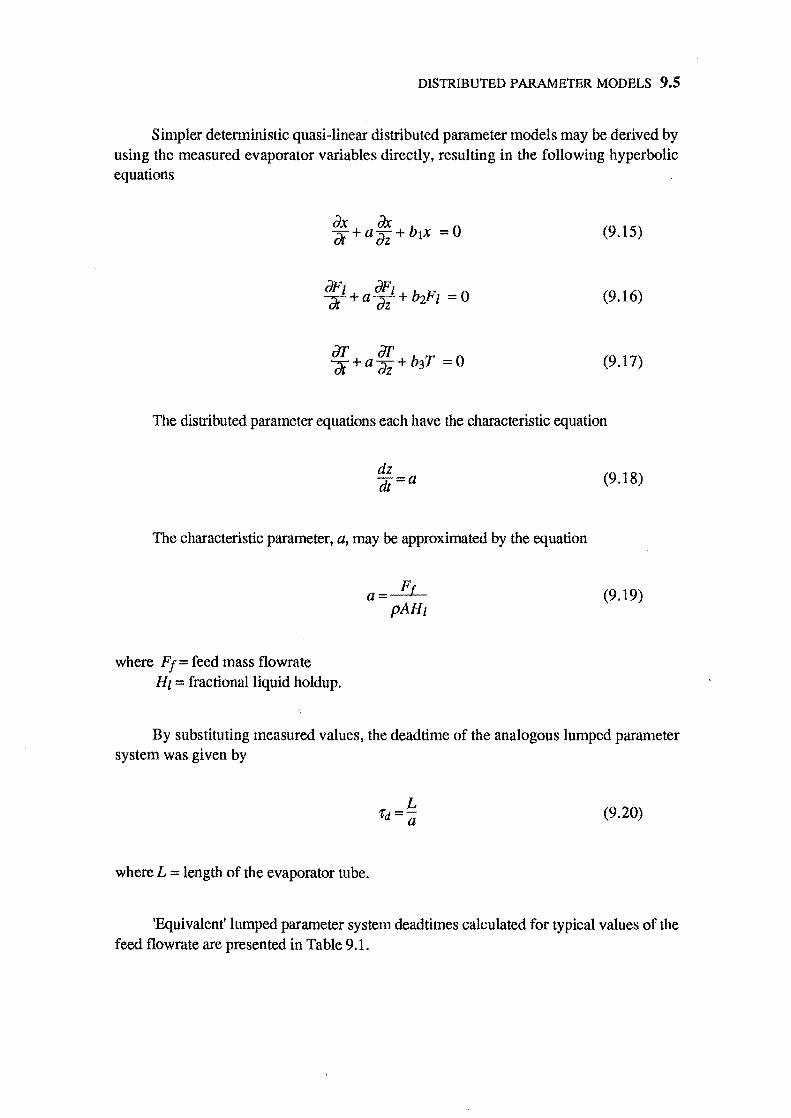
DISTRIBUTED PARAMETER MODELS 9.5
Simpler deterministic quasi-linear distributed parameter models may be derived by using the measured evaporator variables directly, resulting in the following hyperbolic equations
(9.15)
(9.16)
(9.17)
The distributed parameter equations each have the characteristic equation
dz dt =a
The characteristic parameter, a, may be approximated by the equation
where Ff = feed mass flowrate HI = fractional liquid holdup.
a=~ pAHI
(9.18)
(9.19)
By substituting measured values, the deadtime of the analogous lumped parameter system was given by
(9.20)
where L = length of the evaporator tube.
'Equivalent' lumped parameter system deadtimes calculated for typical values of the feed flow rate are presented in Table 9.1.
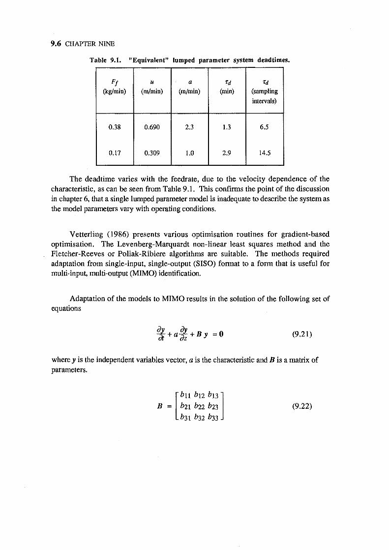
9.6 CHAPTER NINE
Table 9.1. "Equivalent" lumped parameter system deadtimes.
FI u a 'fd 'fd
(kg/min) (m/min) (m/min) (min) (sampling
intervals)
0.38 0.690 2.3 1.3 6.5
0.17 0.309 1.0 2.9 14.5
The dead time varies with the feedrate, due to the velocity dependence of the characteristic, as can be seen from Table 9.1. This confirms the point of the discussion in chapter 6, that a single lumped parameter model is inadequate to describe the system as the model parameters vary with operating conditions.
Vetterling (1986) presents various optimisation routines for gradient-based optimisation. The Levenberg-Marquardt non-linear least squares method and the Fletcher-Reeves or Poliak-Ribiere algorithms are suitable. The methods required adaptation from single-input, single-output (SIS0) format to a form that is useful for multi-input, multi-output (MIMO) identification.
Adaptation of the models to MIMO results in the solution of the following set of equations
(9.21)
where y is the independent variables vector, a is the characteristic and B is a matrix of parameters.
(9.22)
DISTRIBUTED PARAMETER MODELS 9.7
Here it is necessary to solve the matrix exponential. e-Bt• as the method of characteristics predicts
(9.23)
i.e. the characteristic dz dt = a (9.24)
is approximated as L - = a (9.25) 'rd
The matrix exponential is solved by using the Cayley-Hamilton theorem (Astrom and Wittenmark, 1984).
Choice of starting values of the B matrix was difficult. There were two choices:
(i) Use the b values obtained from SISO identification. The result is that the b parameters become the diagonal elements (and hence eigenvalues) of the B matrix.
(ii) Use the best lumped parameter model parameter estimates to provide the initial values by considering these models as approximations for a distributed parameter model.
In practice, neither of these approaches were found to be adequate. The identification was very sensitive to slight changes in the values of the B matrix elements (especially the diagonal elements) and the optimisation became rapidly unstable.
Returning to the SISO approach again. it was thought that it may be possible to concentrate on only one input. with the other inputs considered as forcing inputs to the system. resulting in the solution of an non-homogeneous equation by the method of characteristics.
9.8 CHAPTER NINE
The equation for the characteristic was
dz dt = a (9.26)
approximated as before by
L - = a (9.27) 'l:d
The non-homogeneous equation that has to be solved along the characteristic is
i = B'.y(t,z) + C·yfit) (9.28)
where [
b l 0 0] B' = 0 b2 0 ,
o 0 b3 [
0 C12 C13] C = c2l 0 c23
C3l c32 0
(9.29)
are the parameters to be identified, and the 'forcing' inputs are
yfit) = y(t,O) (9.30)
The results of this approach follow.
Figure 9.1 is typical of the plots of the actual and predicted model outputs. The evaporator output identified is the product concentration. The model used is the linear non-homogeneous distributed model for the plant at an operating point of 2.5±2.0wt% NaNQ3 feed concentration.
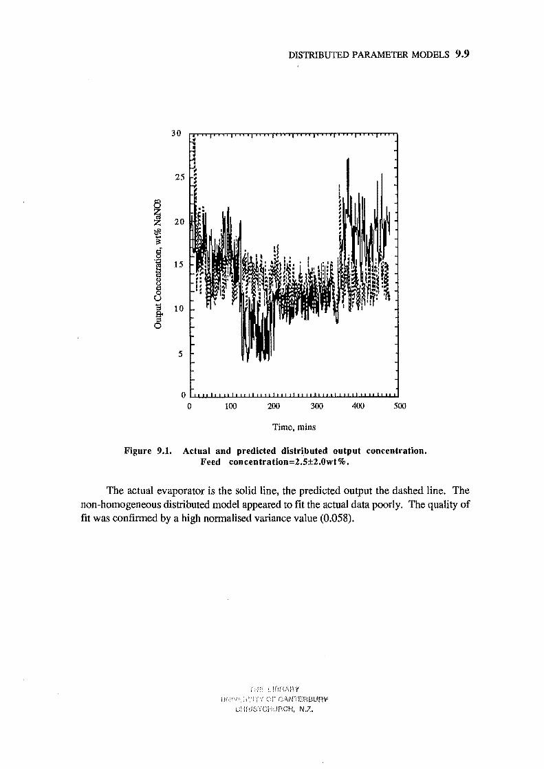
DISTRIBUTED PARAMETER MODELS 9.9
30
25
~ Z 20 ~ !i §
'J:j
f1 15
8 c:: 0 u t:! 10 ~ 0
5
o u.~~~~~~~~~~~~~~~~~ o 100 200 300 400 500
Time, mins
Figure 9.1. Actual and predicted distributed output concentration. Feed concentration=2.5±2.0wt%.
The actual evaporator is the solid line, the predicted output the dashed line. The non-homogeneous distributed model appeared to fit the actual data poorly. The quality of fit was confirmed by a high normalised variance value (0.058).
GlHmnCI1UFICH, N.Z.
9.10 CHAPTER NINE
The minimum normalised variances for the concentration of the product concentrate (Yl), the exit flowrate (Y2) and the exit temperature (Y3) are given in Tables 9.2 and 9.3 for feed temperatures of 20°C and 60°C respectively.
Table 9.2. Minimum Variances for Identification of each output with a linear non-homogeneous distributed model, at 20°C Feed Temperature.
Output Nonnalised Variance
Yl 0.05816
Y2 0.32649
Y3 0.00193
Sum of Normalised
Variances 0.38658
Table 9.3. Minimum Variances for Identification of each output with a linear non-homogeneous distributed model, at 60°C Feed Temperature.
Output ,
Nonnalised Variance
Y1 0.05899
Y2 0.01748
Y3 0.12661
Sum of Normalised
Variances 0.20308
The sum of normalised variances criterion was used to determine the quality of the model fit. The sum of normalised variances criteria for the non-homogeneous distributed parameter models were greater than the best lumped parameter models identified in chapters 7 and 8. The individual normalised variances were also larger than the model variances for the lumped parameter models.
DISTRIBUTED PARAMETER MODELS 9.11
CONCLUSIONS
The identification of simplified detenninistic distributed parameter models was achieved. However, the variances for the non-homogeneous distributed parameter model were larger than the best lumped parameter models identified in the previous chapters. No improvement over the mathematically simpler gain-scheduled models was found. The distributed parameter model was not as good as a gain scheduled model at describing the evaporator behaviour, based on the minimum variance criterion. It would seem that the gain scheduled approach was sufficient to handle the non-linearities of the system - the distributed nature of the evaporator would appear to be less significant by comparison.
ABBREVIA TIONS
MIMO Multi-input, multi-output
SISO Single-input, single-output
SYMBOLS
a Characteristic value for the hyberbolic partial differential equations
A Evaporator tube cross sectional area
b Distributed parameter, associated with initial conditions, to be identified
c Distributed parameter, associated with a forcing input, to be identified
Cf Homogeneous friction factor
Cp Homogeneous mixture heat capacity
D Evaporator tube diameter
FI Feed flowrate
Fg Vapour flowrate
FI Liquid flowrate
hi Local internal heat transfer coefficient from the evaporator steam jacket to the fluid
HI Fractional liquid holdup
L Evaporator tube length
9.12 CHAPTER NINE
Time
T Homogeneous mixture temperature
T g Vapour temperature
T, Liquid temperature
T w Evaporator steam jacket temperature
u Homogeneous mixture velocity
x Mass fraction of the vapour phase
Y 1 concentration (wt%) of product concentrate
Y2 product exit f10wrate
Y3 product exit temperature
z Distance up the evaporator tube
a Void fraction - the volume fraction of the vapour phase
It Latent heat of vaporisation of steam
P Homogeneous mixture density
Pg Vapour density
PI Liquid density
Pw Water liquid density
"Cd Equivalent lumped parameter system deadtime
DISTRIBUTED PARAMETER MODELS 9.13
REFERENCES
Astrom,K.J. and Wittenmark,B., "Computer Controlled Systems: Theory and Design",
Prentice-Hall International, pp2S-27,pp40S-7 (1984).
Carpenter,W.T., Wozny,M.J. and Goodson,R.E., "Distributed Parameter Identification
Using the Method of Characteristics", Trans. ASME, J. Dynamic Systems, Measurement and
Control, Vol. 93, pp73-78 (1971).
Vetterling, W.T., Teukolsky, S.A., Press, w.n. and Flannery, B.P., "Numerical
Recipes", Cam bridge University Press, (1986).

CHAPTER
TEN
CONCLUSION
A range of models of the climbing film evaporator were compared and. contrasted for the specific purpose of developing of industrially-viable process control systems for the climbing film evaporator.
A comparison of two commonly used recursive identification algorithms for linear lumped parameter systems was completed; recursive least squares and recursive extended least squares. The performance of the algorithms was assessed by observing the rate of convergence of the estimated parameters and the bias in the final identified parameter values for simulated systems.
The recursive least squares (RLS) method gave biased parameter estimates for cases with any measurement noise, converging to incorrect values of the system parameters. Recursive extended least squares (RELS) reduced, but did not eliminate this parameter bias, giving unreasonable parameter estimates at higher noise values. Both identification methods used a UD factorisation algorithm and were robust for inappropriate choices of system deadtime. Accurate estimates of dead time were obtained from either method.
The simplest models that were identified for the evaporator were global black-box linear models.
Simple global linear models of the climbing film evaporator, with the parameters of these models identified by implementing the afore mentioned recursive algorithms, did not reproduce its behaviour over the full operating range, and increasing the model order did not offer significant improvement.
10.1
10.2 CHAPTER TEN
Separate multi-input, multi-output (MISO) identification gave the best results based on the minimum sum of normalised variances criterion, of the three types of global linear models proposed - single overall dead time with equal model orders, single overall deadtime with differing model orders and separate identification of each output.
There was little or no improvement to be gained from RELS identification over RLS identification. In fact, separate MISO identification showed a marginal increase in the sum of nOlmalised variances in some cases using RELS instead of RLS.
A difference between the identified global models at the two feed temperature setpoints considered was also apparent. Both the model deadtimes and orders changed.
Gain-scheduled linear models were identified in an attempt to compensate for system non-linearity and the distributed nature of the system. These simple linear gainscheduled models, which made the equivalent time constants and dead-times functions of the plant operating conditions, provided reasonably effective models of the climbing film evaporator without the complexity of the distributed parameter approach.
A comparison with the identified global models indicated the variances had been approximately halved. Of the three types of models, separate MISO identification did not necessarily give the best results. The simplest model type identified was a model with a single overall deadtime and order.
RLS identification with the simplest model type was superior for many operating ranges. There was little improvement to be gained from RELS identification over RLS identification.
Finally, full distributed parameter models were derived for the evaporator, and their parameters identified. The set of partial differential equations describing the climbing film evaporator are of the hyperbolic type. The method of characteristics was employed within a non-linear least squares optimisation scheme to solve this parameter identification problem.
The distributed parameter model of the climbing film evaporator was limited by the assumption of homogeneous flow, yet remained too unwieldy to implement the optimisation scheme successfully. The identification of simplified deterministic distributed parameter models was achieved, but gave no improvement over the mathematically simpler gain-scheduled models.
CONCLUSION 10.3
In conclusion the best models identified, for the purpose of producing an industrially-viable control system, were gain-scheduled linear models, based on the minimum output least square error cliterion. The gain-scheduled models also have the advantage that they are relatively easier to implement than distributed parameter models.
ABBREVIATIONS
MISO Multi-Input. Single-Output
RLS Recursive Least Squares
RELS Recursive Extended Least Squares


APPENDICES

APPENDIX
I
CLIMBING FILM EVAPORATOR OPERA TING PROGRAM
In which the operating program of the climbing film evaporator system is described. The functions of the program are listed and implementation and installation of the program detailed.
1.1 - FUNCTIONS
The operating program to run the climbing film evaporator was written to allow data collection and control of the climbing film evaporator and the devices associated with it. The program was capable of performing the following functions:
• An automatic startup sequence which handled the transition from manual to automatic control of the climbing film evaporator in an orderly manner.
• Data collection, logging and control by a set of routines that collected, logged to file and displayed process data on the operator terminal in graphical form. Commands input from the keyboard permitted the operator to alter the climbing film evaporator setpoints.
• An automatic shutdown sequence which performed an orderly shutdown of the climbing film evaporator.
1.1
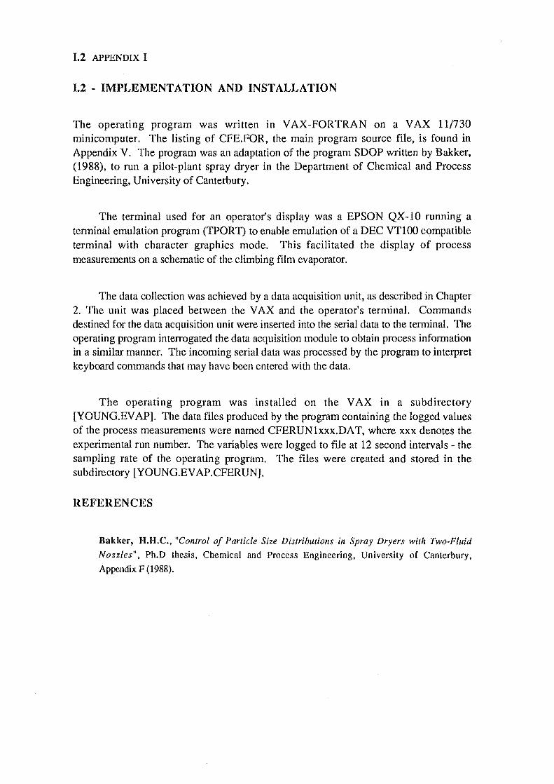
1.2 APPENDIX I
1.2 - IMPLEMENTATION AND INSTALLATION
The operating program was written in VAX-FORTRAN on a VAX 11/730 minicomputer. The listing of CFE.FOR, the main program source file, is found in Appendix V. The program was an adaptation of the program SDOP written by Bakker, (1988), to run a pilot-plant spray dryer in the Department of Chemical and Process Engineering, University of Canterbury.
The terminal used for an operator's display was a EPSON QX-IO running a terminal emulation program (TPORT) to enable emulation of a DEC VT100 compatible terminal with character graphics mode. This facilitated the display of process measurements on a schematic of the climbing film evaporator.
The data collection was achieved by a data acquisition unit, as described in Chapter 2. The unit was placed between the VAX and the operator's terminal. Commands destined for the data acquisition unit were inserted into the serial data to the terminal. The operating program interrogated the data acquisition module to obtain process information in a similar manner. The incoming serial data was processed by the program to interpret keyboard commands that may have been entered with the data.
The operating program was installed on the VAX in a subdirectory [YOUNG.EV AP]. The data files produced by the program containing the logged values of the process measurements were named CFERUN lxxx.DA T, where xxx denotes the experimental run number. The variables were logged to file at 12 second intervals - the sampling rate of the operating program. The files were created and stored in the subdirectory [YOUNG.EV AP.CFERUN].
REFERENCES
Bakker, H.H.C., "Control of Particle Size Distributions in Spray Dryers with Two-Fluid
N ozzles", Ph.D thesis, Chemical and Process Engineering. Un iversity of Canterbury,
Appendix F (1988).
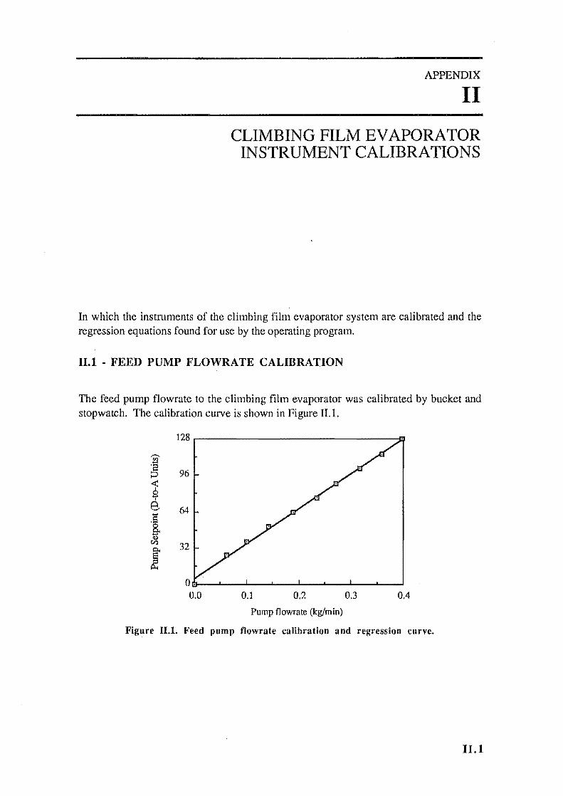
APPENDIX
II
CLIMBING FILM EVAPORATOR INSTRUMENT CALIBRATIONS
In which the instruments of the climbing film evaporator system are calibrated and the regression equations found for use by the operating program.
11.1 - FEED PUMP FLOWRATE CALIBRATION
The feed pump flowrate to the climbing film evaporator was calibrated by bucket and stopwatch. The calibration curve is shown in Figure 11.1.
128.---------------------------~
96
64
32
OG·-----~-----~--~--~~--~--~--~ 0.0 0.1 0.2 0.3 0.4
Pump flowrate (kg/min)
Figure 11.1. Feed pump flowrate calibration and regression curve.
ILl
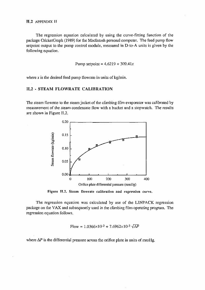
II.2 APPENDIX II
The regression equation calculated by using the curve-fitting function of the package CricketGraph (1989) for the MacIntosh personal computer. The feed pump flow setpoint output to the pump control module, measured in D-to-A units is given by the following equation.
Pump setpoint = 4.6219 + 309.41x
where x is the desired feed pump flowrate in units of kg/min.
11.2 • STEAM FLOWRATE CALIBRATION
The steam flowrate to the steam jacket of the climbing film evaporator was calibrated by measurement of the steam condensate flow with a bucket and a stopwatch. The results are shown in Figure 11.2.
0.20 r------------------,
0.15
0.10
0.05
0.00 J!I.. _--'-_--'-_--'-_......L.._--'-_-'--_--'-_....J
o 100 200 300 400
Orifice plate differential pressure (mmHg)
Figure 11.2. Steam flowrate calibration and regression curve.
The regression equation was calculated by use of the LINPACK regression package on the VAX and subsequently used in the climbing film operating program. The regression equation follows.
Flow = 1.0366xlO-2 + 7.6962xlO-3 ...JM
where AP is the differential pressure across the orifice plate in units of mmHg.
INSTRUMENT CALlBRA TlONS 11.3
11.3 . OUTPUT FLOWRATE CALIBRATIONS
The differential pressure above an orifice plate was measured for varying output flowrates of concentrated product and condensate from the condenser stream, measured by bucket and stopwatch. These calibration curves are shown in Figures II.3 and II.4.
0.4 ,...---------------:::rn~---,
0.3
0.2
0.1
0.0 L...L-..L--'--....L----L...--I...--L---lL-I..-..L-..L.---'---'----'----'
800 1000 1200 1400 1600 1800 2000 2200
Differential pressure (A-to-D Units)
Figure 11.3. Product flowrate calibration and regression curve.
0.10 ,...---------------""""7"---,
0.08
0.06
1050 1150 1250 1350
Differential pressure (A-to-D units)
Figure 11.4. Condensate flowrate calibration and regression curve.
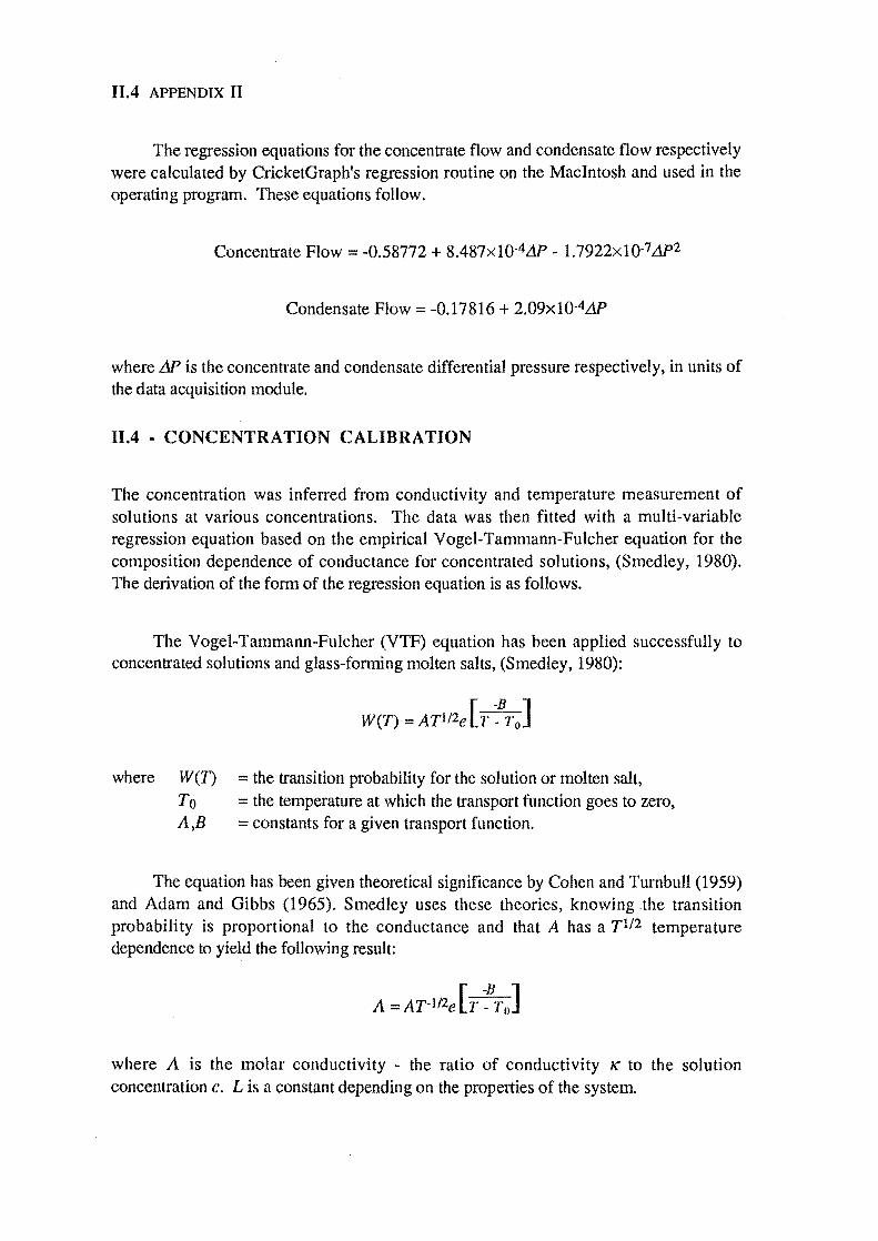
II.4 APPENDIX II
The regression equations for the concentrate flow and condensate flow respectively were calculated by CricketGraph's regression routine on the MacIntosh and used in the operating program. These equations follow.
Concentrate Flow = -0.58772 + 8.487xlO-4L1P - 1.7922xlO-7 L1P2
Condensate Flow = -0.17816 + 2.09xlO-4L1P
where L1P is the concentrate and condensate differential pressure respectively, in units of the data acquisition module.
II.4 - CONCENTRATION CALIBRATION
The concentration was inferred from conductivity and temperature measurement of solutions at various concentrations. The data was then fitted with a multi-variable regression equation based on the empirical Vogel-Tammann-Fulcher equation for the composition dependence of conductance for concentrated solutions, (Smedley, 1980). The derivation of the form of the regression equation is as follows.
The Vogel-Tammann-Fulcher (VTF) equation has been applied successfully to concentrated solutions and glass-forming molten salts, (Smedley, 1980):
where W(D = the transition probability for the solution or molten salt, To = the temperature at which the transport function goes to zero, A ,8 = constants for a given transport function.
The equation has been given theoretical significance by Cohen and Turnbull (1959) and Adam and Gibbs (1965). Smedley uses these theories, knowing the transition probability is proportional to the conductance and that A has a Ti/2 temperature dependence to yield the following result:
A = AT-l12e L· ~BTJ where A is the molar conductivity - the ratio of conductivity 1( to the solution concentration c. L is a constant depending on the properties of the system.
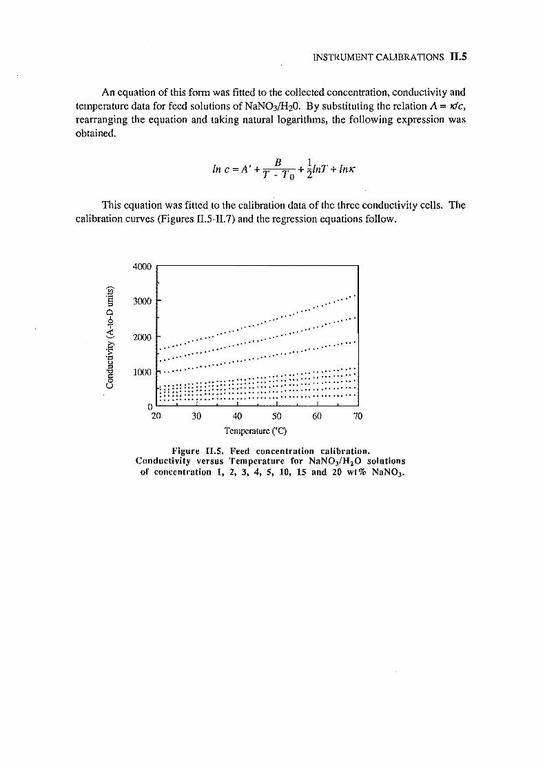
INSTRUMENT CALIBRATIONS 11.5
An equation of this form was fitted to the collected concentration, conductivity and temperature data for feed solutions of NaN03/HzO. By substituting the relation A = 1(/c, rearranging the equation and taking natural logarithms, the following expression was obtained.
In c = A' + T ~ T 0 + !lnT + In 1(
This equation was fitted to the calibration data of the three conductivity cells. The calibration curves (Figures II.S-II.7) and the regression equations follow.
4000.------------------------------.
3000
2000 , .' . ,,' "
".' " . ' '
.' ' ......
." "" ,.' "t " •• " .. - ,." ... "
to- ,0· " ... .. ".
.. ' " '
.. ' " '
" .. " ." .. " ' . ... .". ,," "'I' ..
.... -.... - ..
" . .. . ' '
" ' ." ",,-
..... " ,. " ,,~
1000 h t~ .". "", ... ,,
... "_. ..... " .. ...... . "" .. "." .. - : ............ " ••• tt ." •••• '" ••••• "'::: ::: ":::: ::: •••••• " ••• " •• "
::: ::: ::::: ::: ::::: ::::: ::: ::::: ::: ::::: ::: :::::: ..... '" ....... ' ....... . o~~--~--~~--~--~~--~--~~
20 30 40 50 60 70
Temperature eC)
Figure II.S. Feed concentration calibration. Conductivity versus Temperature for NaN03/H20 solutions
of concentration 1, 2, 3, 4, S, 10, 1S and 20 wt% NaN03 •
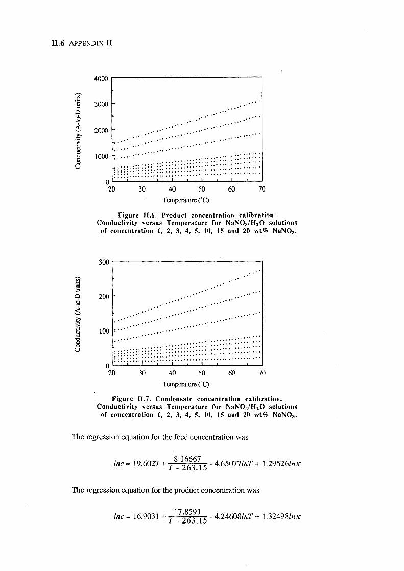
II.6 APPENDIX II
4000~----------------------------'
3000 r- .. ' · .' • to •• .. ' .. , f 111 • to' •••
• to • .. " .. . ,... . .. ,_. 2000 r- .' •• ' .' • .' •. , .' •• '
• .. • ... to .. " "
.... ' •• to to . ' •• .. • • .. to ... to ........ .
•• - •• - ,a.-to .. ' .... IJ ••••• to ••• to ... ".. .. , ...
1000 r: ............ .. ..... .. .. ' ....... ::: ::: ::::: ::: ~~~ ~~ ::: ::::::
~ H ~n H~ l~ ~~~ ~~~ ~~ /:: ::: ::;:: ::: .... ; ........ . O~~--~--~~---L--~~---L--~~
20 30 40 50 60 70
Temperature rC) Figure 11.6. Product concentration calibration.
Conductivity versus Temperature ror NaN03/HzO solutions or concentration 1, 2, 3, 4, 5, 10, 15 and 20 wt% NaN03 •
300~------------------------------~
· . . . . ' .. 200 - ..
.' .. lO- ...- .
.' . · .. ,.
100
· . . ' .. .. ,
. ' .. lO·- . " ....
..
· .' 1··- . . ' . ..... · lO.-·
... ,.' . . . • to ••
a .....
.. '
..t .. I'· .
.... to .' . . ....
••• I • • lO •• to."
. . ' :: : : : : : : :: :: .. : : :: : :: : : : .. ' :.:. :.:.:.' :.':.'~ ~~ ~~~ ~~~!~ ~~~:: ::: ::::: ::: :::: ......... .
.. ••• lO ••• " ••• lO •• lO-· ........ to. to i ........ to • i ......... ; . I O~~--~--~~---L--~--'-----'---~~
20 30 40 50 60 70
Temperature rC) Figure 11.7. Condensate concentration calibration.
Conductivity versus Temperature ror NaN03/HzO solutions or concentration 1, 2, 3, 4, 5, 10, 15 and 20 wt% NaN03 •
The regression equation for the feed concentration was
8.16667 Inc = 19.6027 + T _ 263.15 - 4.65077lnT + 1.295261nK'
The regression equation for the product concentration was
17.8591 Lnc= 16.9031 +T _ 263.15 - 4.246081nT+ 1.32498LnK'
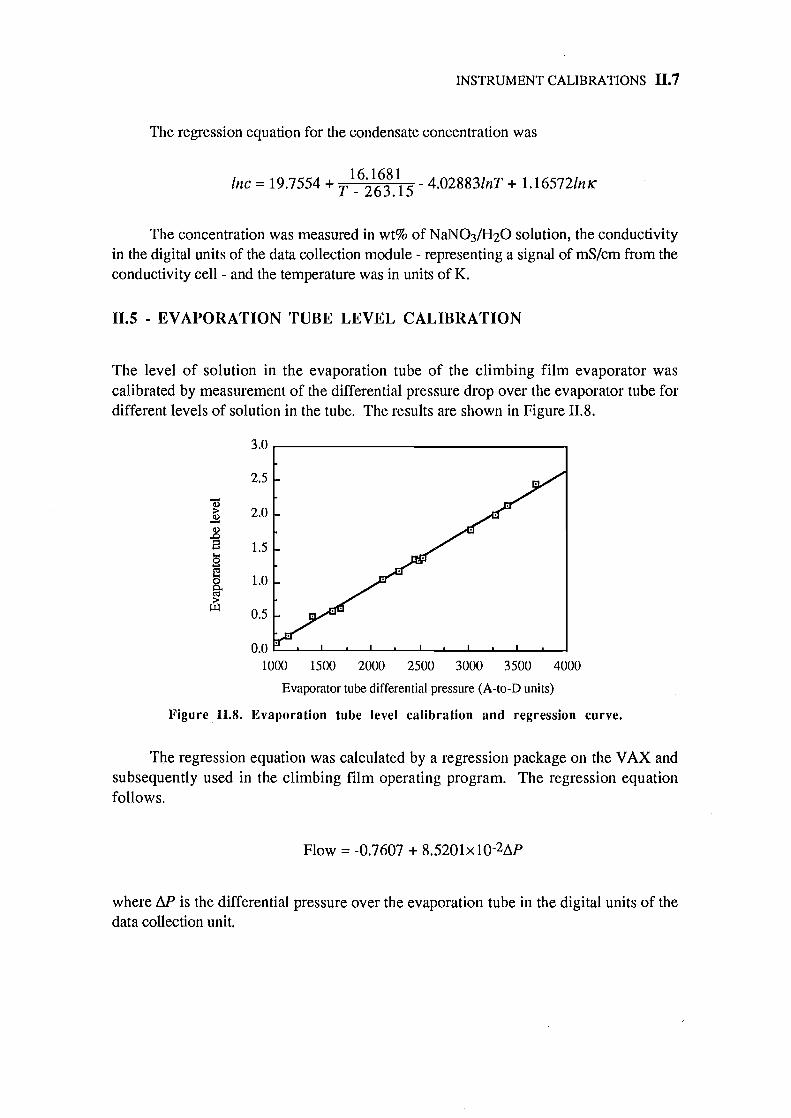
INSTRUMENT CALI BRA TIONS 11.7
The regression equation for the condensate concentration was
16.1681 Inc = 19.7554 + T _ 263.15 - 4.02883/nT + 1.165721nK"
The concentration was measured in wt% of NaN03/H20 solution, the conductivity in the digital units of the data collection module - representing a signal of mS/cm from the conductivity cell - and the temperature was in units of K.
11.5 - EVAPORATION TUBE LEVEL CALIBRATION
The level of solution in the evaporation tube of the climbing film evaporator was calibrated by measurement of the differential pressure drop over the evaporator tube for different levels of solution in the tube. The results are shown in Figure 11.8.
3.0
2.5
~ &> 2.0 -~ 1.5
~ ~ 1.0
& 0.5
1000 1500 2000 2500 3000 3500 4000
Evaporator tube differential pressure (A-to-D units)
Figure 11.8. Evaporation tube level calibration and regression curve.
The regression equation was calculated by a regression package on the VAX and subsequently used in the climbing film operating program. The regression equation follows.
Flow = -0.7607 + 8.5201xlO-2i1P
where M is the differential pressure over the evaporation tube in the digital units of the data collection unit.
11.8 APPENDIX II
REFERENCES
Adam, G. and Gibbs, J.H., "On the temperature dependence of cooperative relaxation
properties in glass10rming/iquids", J. Chern. Phys., Vol. 43, pp134-146 (1965).
Cohen, M.H. and Turnbull, D., "Molecular transport in liquids and glasses", J. Chern.
Phys., Vol 31. ppl164-1169 (1959).
CricketGraph, Version 1.3.1, Cricket Software, 40 Valley Stream Parkway,
Malvern PA 19355, (1989).
Smedley, S.I., "The Interpretation of Ionic Conductivity in Liquids", Plenum Press, New
York, Chapter 3 (1980).
APPENDIX
III
ELECTRONIC CIRCUIT DIAGRAMS
In which the electronic circuit diagrams are presented for various instruments associated with the climbing film evaporator - as described in Chapter 2, Apparatus. The circuits were designed and built by the Chemical and Process Engineering Department, and commissioned and calibrated by the author.
I1I.!
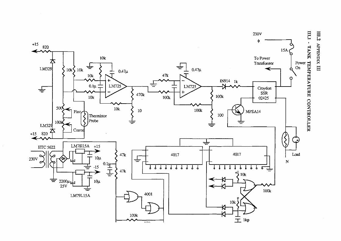
+15 820
LM329
22001l 25V I
,
LM79L15A
10k
0.1 .:.l-
47k
I < 47k
I
230V
<I>
To Power Transfonner
Croydon SSR
02425
MPSA14
~------~----~I ~I ----~--------~
4017 4017
J J J J J J ! J J J A A A A A tAt t
.I.. 1kp
..... ..... ..... ==
r )00'0. N
15A (" 1-3 ~ ;l> :z ~ 0 .....
~~wer i :><: ---"'t:I r%l ::::= ;l> 1-3 0 ::::= r%l ("":l
0 :z 1-3 ::::= 0 r" r" t!l ::::=
Load
N
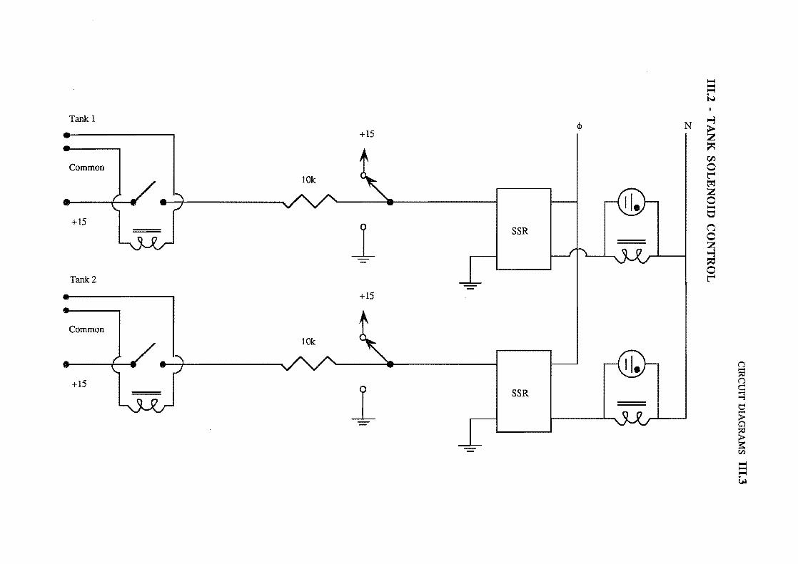
CIR
CU
IT D
IAG
RA
MS
111.3
111.2 -T
AN
K SO
LE
NO
ID C
ON
TR
OL
z-------------------------------~--~----------------~
\f1
...... +
~ s 8
\f1
...... +
II
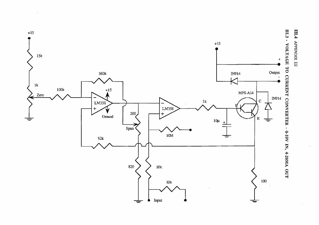
111.4 A
PP
EN
DIX
III
111.3 -V
OL
TA
GE
TO
CU
RR
EN
T C
ON
VE
RT
ER
-O
-IOV
IN, 4-20M
A O
UT
+
~' o
l.()
'+ --
.....
.q-...... « I
til
l.() ,..., +
~
.q-......
~ II
U
'-----III
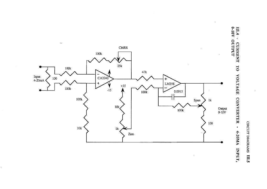
CIR
CU
IT D
IAG
RA
MS
III.S
IlIA
w
CU
RR
EN
T
TO
V
OL
TA
GE
C
ON
VE
RT
ER
w
4-20M
A
INP
UT
, O
-IOV
O
UT
PU
T
8 ......
Irl ...... ,
..;.:
8 ......
~6 =
...... 0
0
8 ......
..;.: o ......
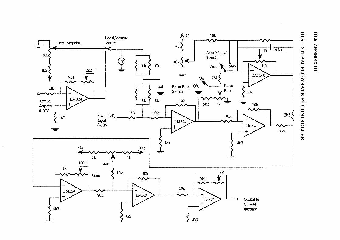
~ ~
10k ~ ~
Local/Remote ~ ~v ~ ~ u.. ~
Local Setpoint Switch I ~ 00
Auto-Manual I ~-15 6.8J.l. ~ '"tI m Switch
~ Z ;> t:1 ~ -~ ~
..... 1k2 .1 2k2 --'-- , ~ 1. )''0 ICA~
..... t"'" ..... 0 ~
Reset Rate ~ '~ Keset ~: ~ ;>
Switch _ Rate ~ ~
10k I - - - -....l- ....I- "0 ~
2k 10k n 10k 0
SteamDP Z Input
~ ~
O-lOV 0 t"'" t"'" ~ ~ j 4k7 < 4k7
-15 +15
lOOk Zero
~lOk~ 2k Gain
10k
~-~ Output to Current Interface
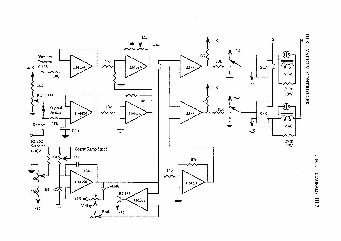
Vacuum
+15
Remote
o---l Remote Setpoint O-lOV
-15
IN4148
10k
TO. I J.1.
Coarse Ramp Speed
1M
1M +15
Gain
4k7
~
+15
~
10k
10k
)0004 )0004
$ Nt"'" ~
+15 .- <: > n c:: c:: ~ n 0 z 0-3 ::c 0 t"" t"" t'!1 ::c
I SSR1 rWI I
, -15 ~
2x2k lOW
\.l ~ \.l c: ::j 0 ,.... E; :;:0
~ CI.l
1000II 1000II ~ ........
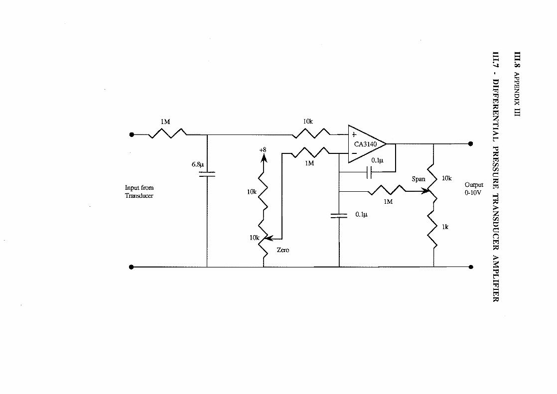
I1I.S A
PP
EN
DIX
III
111.7 -D
IFF
ER
EN
TIA
L P
RE
SS
UR
E T
RA
NS
DU
CE
R
AM
PL
IFIE
R
:::I. ...... d
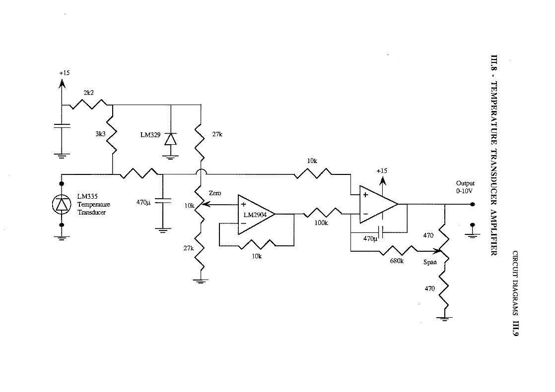
CIR
CU
IT D
IAG
RA
MS
111.9
IlLS
. T
EM
PE
RA
TU
RE
TR
AN
SD
UC
ER
AM
PL
IFIE
R
.!.4 t-C
'l
II ,...;
II H
I' gj M
::g
::t 0
....l t-"'"
$:I ~ i ~
M
~ ~1 j~E--
~
HI!
,...;
II +

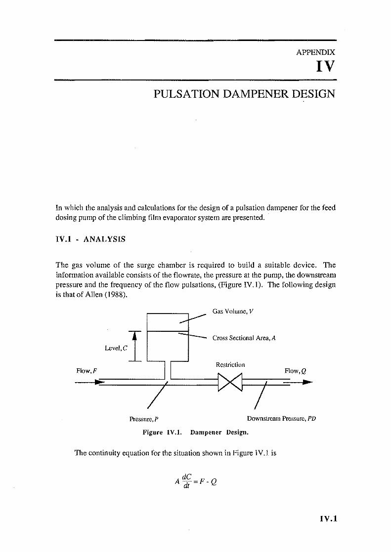
APPENDIX
IV
PULSATION DAMPENER DESIGN
In which the analysis and calculations for the design of a pulsation dampener for the feed dosing pump of the climbing film evaporator system are presented. '
IV.I • ANALYSIS
The gas volume of the surge chamber is required to build a suitable device. The information available consists of the flowrate, the pressure at the pump, the downstream pressure and the frequency of the flow pulsations, (Figure IV.l). The following design is that of Allen (1988).
Gas Volume, V
Level,C I Cross Sectional Area, A
Restriction Flow,F Flow,Q
iii!: ....
Pressure, P Downstream Pressure, PD
Figure IV.1. Dampener Design.
The continuity equation for the situation shown in Figure IV.l is
de A(ft=F-Q
IV.I
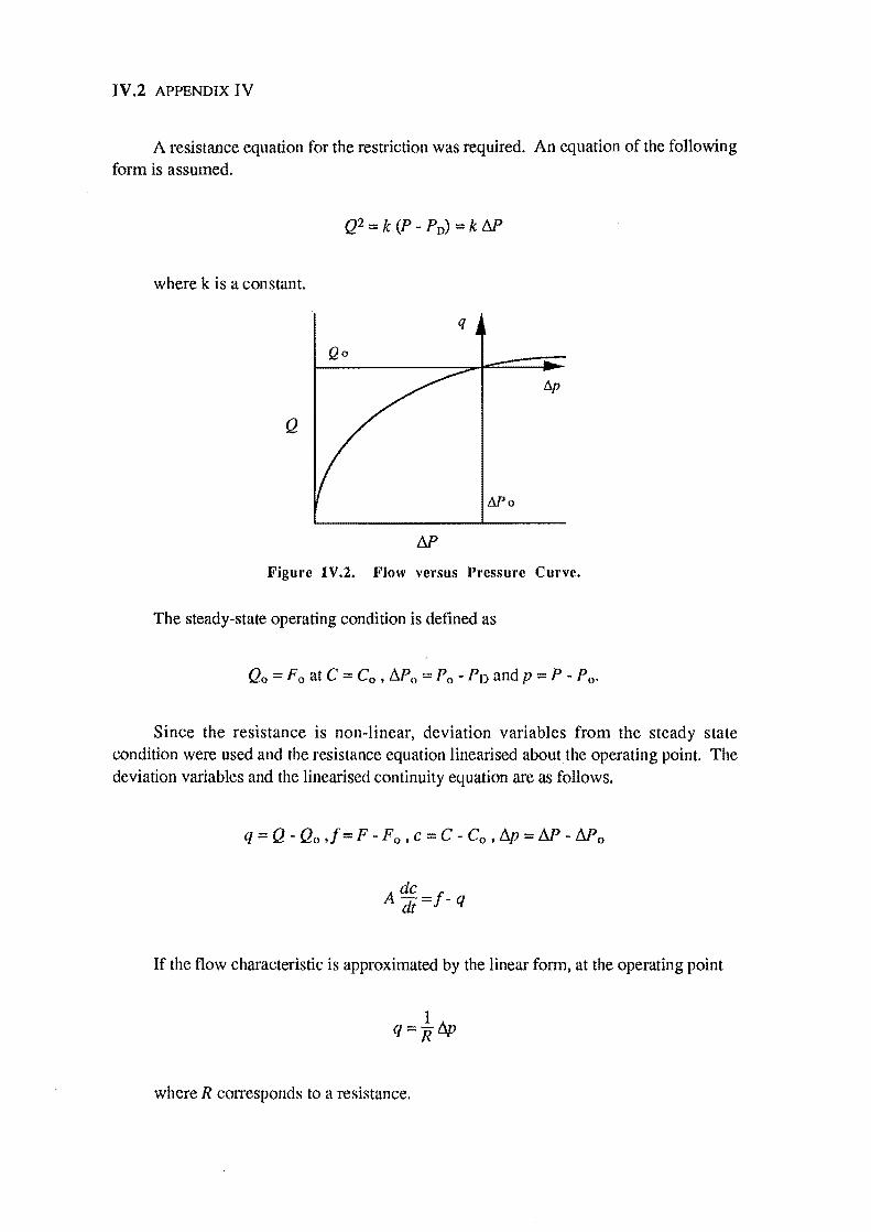
IV.2 APPENDIX IV
A resistance equation for the restriction was required. An equation of the following form is assumed.
where k is a constant.
q
Qo
ll.p
Q
M'o
Figure IV.2. Flow versus Pressure Curve.
The steady-state operating condition is defined as
Qo = F 0 at C = Co , AP 0 = Po - PD and p = P - Po.
Since the resistance is non-linear, deviation variables from the steady state condition were used and the resistance equation linearised about the operating point. The deviation variables and the linearised continuity equation are as follows.
q = Q - Qo ,f = F - F 0 , e = C - Co , Ap = AP - AP 0
de A dt =/ - q
If the flow characteristic is approximated by the linear form, at the operating point
where R corresponds to a resistance.
PULSATION DAMPENER DESIGN IV.3
The slope of this line is q/llP = l/R and must be the same as the slope of the characteristic at the point (M o,Qo). This gives
Now Q2 = k M thus 2QdQ = k d(M)
Rearranging then gives
At the operating point
~I -~- Qo2 -~ d(M) ° - 2Qo - 2MoQo - 2Mo
So the linear resistance is given by
R_ 2Mo - Qo
Returning to the continuity equation
dc ~ Adt=f-q=f- R
The gas law P V = n R' T is introduced. Differentiating with respect to time yields
Now
This gives
So
dV= -A de.
dV de de di= -A di= -A dt
P A dc= V dP = V tiE dt dt dt
IV.4 APPENDIX IV
Substituting into the continuity equation
Now Ap == M - M 0 == (P - PD) - (Po - PD) == P - Po == P
So ~-~ dt - dt
And V d(i3.p) -1-~ P dt - R
R V d(~r) + i3.p ==RI
The time constant is defined as 'r - Rp V and the Laplace transform of the above equation is taken.
('r S + 1) Ap == R 1
but i3.p == R q and Ap == R q
Thus the relationship between q and/is first order with time constant 'r and unity gain.
For a sinusoidal flow F given by
F == F 0 (1 + sin rot)
So that I==Fosinrot
The amplitude ratio of the flows (Figure IV.3) will be given by
PULSATION DAMPENER DESIGN IV.S
F
f
I?igure IV.3. Amplitude ratio of the flows.
For the output amplitude to be 10% of the input amplitude, (J)'f = 10 and the required time constant is
where (J) is the angular frequency of the pump.
Hence the required air volume in the dampener, V, is given by
IV.2 • CALCULATIONS
V=_10_~ (J)R
For a downstream pressure of 20kPa, a pump pressure of SOkPa and a flowrate of IVmin, the resistance is
R - 2 P - PD _ 2 (0.5 - 0.2) x 102
- Qo - x 1 60
= 3600 Pa.s.m-3
IV.6 APPENDIX IV
For a pump angular frequency of 1 stroke per minute, the required volume for the pulsation dampener is
V= 1O P o= 10 x 0.5 X 103
(0 R 2" x 3600
= 2.211itres.
REFERENCES
Allen, R.M., Internal Memo, Department of Chemical and Process Engineering, University of
Canterbury, 28 December (1988),
APPENDIX
V
PROGRAM LISTINGS AND DATA CATALOGUE
In which the listings of the programs and data found on the high density floppy disks labelled "PROGRAMS & DATA" are catalogued. The subroutines comprise the operating program for the climbing film evaporator, the lumped parameter identification program, the distributed parameter identifcation program and the data acquisition unit program.
V.I - CLIMBING FILM EVAPORATOR OPERATING PROGRAM
The various sections of the climbing film evaporator operating program are listed below. The subroutines have been grouped into a number of source files. The main program source file is CFE.FOR. The program was written in VAX-FORTRAN.
CFE.FOR - Main Program Source File
COMMON.FOR - The program-wide common block
COLLECTDATA.FOR - The data collection routines
COMMAND.FOR - The keyboard command interpreter
CONVERSION.FOR - The unit conversion routine
LOGDATA.FOR - Data logging routines
QXSCREEN.FOR - EPSON QXlO Screen Initialisation and Updating
QXSCREENSUB.FOR - Screen drawing routines for the EPSON QXlO
V.I
V.2 APPENDIX V
V.2 • LUMPED PARAMETER IDENTIFICATION PROGRAM
The following is a listing of the various sections of the VAX-FORTRAN program used to identify lumped parameter models of the climbing film evaporator. The subroutines are grouped into a number of source files. The main program source file is UDUMISO.FOR.
UDUMISO.FOR - Main Program Source File
INITIAL. FOR - Initialisation of variables
MA TRIX.FOR - Subroutines of matrix operations
MODELREAD.FOR - A subroutine to read model parameters from a file
RMETHODS.FOR - A subroutine of auxiliary recursive regression methods
TYPECAST.FOR - A subroutine to determine the model structure
WEIGHfING.FOR - A subroutine to weight variables in the identification
V.3 • DISTRIBUTED PARAMETER IDENTIFICATION PROGRAM
The VAX-FORTRAN program MRQFIT.FOR evaluates the parameters of a distributed model by the Levenberg-Marquardt Non-linear Least Squares algorithm, in conjunction with the Method of Characteristics.
V.4 • DATA ACQUISITION UNIT PROGRAM
The assembly listing in Motorola 6809 code for the data acquisition unit used with the climbing film evaporator is stored in the source file EVAP.MIC.
V.S • CLIMBING FILM EVAPORATOR DATA
The data collected from the climbing film evaporator, and used for identification purposes is stored in the following source files:
CFERUN08.DAT, CFERUNlO.DAT, CFERUNl1.DAT, CFERUN13.DAT,
CFERUN14.DAT, CFERUN16.DAT, CFERUN19.DAT, CFERUN24.DAT,
CFERUN30.DAT
APPENDIX
VI
IFACPAPER
The following is the text of the paper, based on this work, accepted for presentation at the 12th World Congress of the Intenational Federation of Automatic Control to be held at the Sydney Convention and Exhibition Centre, Darling Harbour, Sydney, Australia, from the 19th to the 23rd of July, 1993.
1
2 APPENDIX VI
Multi-Input, Multi-Output Identification of a Pilot-Plant Climbing Film Evaporator
R.M. Allen 1 and B.R. Y oung2
1. Department of Chemical and Process Engineering, University of Canterbury, Christchurch, New Zealand
2. Department of Chemistry, University of Technology, Sydney, Australia
Keywords: System Identification, Mathematical Modeling, Distributed Parameter Models
Abstract: The major aim of this research was to investigate the modeling and control of a 25 kW, 13.6litres/hour pilot-plant climbing film evaporator concentrating a sodium nitrate solution. This paper reports on a comparison of a range of models of the climbing film evaporator for the specific purpose of developing and designing industrially-viable process control systems. The simplest models of the evaporator were global linear lumped parameter models. Gain-scheduled linear lumped parameter models were identified to compensate for system non-linearity. Finally, full distributed parameter models were derived for the evaporator, and their parameters identified.
1. INTRODUCTION
A climbing film evaporator is a typical distributed parameter system, characterised by its inputs, outputs and system states being dependent not only on time but also on spatial position, up the height of the evaporator tube. For a rigourous description, the evaporator should be modeled by a set of partial differential equations in space and time. However the theory for the identification of model parameters and for the design of controllers, is much less developed than is the case for systems described by ordinary differential equations. Non-linearity emphasises this contrast.
There are two major approaches in the modeling and identification of distributed parameter systems.
The first approach consists of initially lumping the parameters of the distributed parameter system model and applying the identification and control methods for lumped parameter systems to the resulting ordinary differential equations. This is usually the first step in the identification of distributed parameter systems. The simplest type of model description is a linear model where the parameters of the model are time-invariant. These models are often linearisations of non-linear systems and they idealise the real process, but they give good results in many situations.
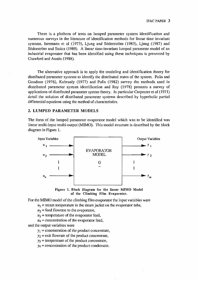
IFAC PAPER 3
There is a plethora of texts on lumped parameter system identification and numerous surveys in the literature of identification methods for linear time invariant systems, Isermann et al (1973), Ljung and Soderstrom (1983), Ljung (1987) and Soderstrom and Stoica (1989). A linear time-invariant lumped parameter model of an industrial evaporator that has been identified using these techniques is presented by Crawford and Austin (1988).
The alternative approach is to apply the modeling and identification theory for distributed parameter systems to identify the distributed states of the system. Polis and Goodson (1976), Kubrusly (1977) and Polis (1982) survey the methods used in distributed parameter system identification and Ray (1978) presents a survey of applications of distributed parameter system theory. In particular Carpenter et al (1971) detail the solution of distributed parameter systems described by hyperbolic partial differential equations using the method of characteristics.
2. LUMPED PARAMETER MODELS
The form of the lumped parameter evaporator model which was to be identified was linear multi-input multi-output (MIMO). This model structure is described by the block diagram in Figure 1.
'abies Input Van
u 1
Output
.... .... EVAPORATOR .... MODEL ....
I G I I - I
.... -Figure 1. Block Diagram for the linear MIMO Model
of the Climbing Film Evaporator.
Variables
y 1
For the MIMO model of the climbing film evaporator the input variables were ul = steam temperature in the steam jacket on the evaporator tube, U2 = feed flowrate to the evaporator, u3 = temperature of the evaporator feed, U4 == concentration of the evaporator feed,
and the output variables were Yl == concentration of the product concentrate, Y2 == exit flowrate of the product concentrate, Y3 == temperature of the product concentrate, Y4 == concentration of the product condensate.
4 APPENDIX VI
The identification methods used to identify the parameters of this model were recursive least squares (RLS) and recursive extended least squares (RELS). These recursive methods were built about a un factorisation algorithm, Biermann (1977), for numerical stability. The methods are known to exhibit biased results in the presence of large noise signals contaminating the output, i.e. they converge to incorrect values of the system parameters. The recursive least squares method gave biased parameter estimates for cases with any measurement noise, converging to incorrect values of the system parameters. Recursive extended least squares reduced, but did not eliminate this parameter bias, giving unreasonable parameter estimates at high noise values. Both identification methods were robust for inappropriate choices of system deadtime.
The methods also required an adequate number of samples before the parameter estimates converged to their final values from the initial guesses. Generally this was of order 1000 samples of all the input and output variables. The choice of sample rate was also important to avoid undesirable effects such as aliasing (Astrom and Wittenmark, 1984). The sample rate chosen was once every 12 seconds, small enough to avoid aliasing problems yet sufficiently large to overcome measurement delays. This implied an experiment duration of 3 hours 20 minutes to collect 1000 samples.
The experiments performed took the form of two 23 factorial experiments (Montgomery, 1984) with a single replicate, each at different input feed temperatures. An independent pseudorandom binary sequence or PRBS (Soderstrom and Stoica, 1989) was superimposed on each of the following inputs - steam temperature, feed flowrate and feed concentration. The PRBS on the steam temperature was obtained by altering the steam flowrate to the steam jacket on the evaporator tube. The PRBS on the feed concentration was afforded by switching between the two feed tanks which contained solutions of two different concentrations.
The above constraints lead to two experiments consisting of four blocks/trials each consisting of four runs at a particular operating points. These runs were randomised within each trial. The duration of each run was 8 hours - determined by the feed flowrate and feed tank size. This resulted in 19200 measurements of four input and four output variables for the identification of the selection of models of the evaporator.
IFAC PAPER 5
2.1. Global Models
The simplest global model of the climbing film evaporator was one which had a single overall deadtime across all die inputs and outputs with model orders equal. This model could easily be extended to the case with a single overall dead time but with the best combination of model orders and the further case where the five MISO systems were considered separately.
The minimum variance criterion was used to choose the most appropriate model. The model variances were normalised by the span of the output variable concerned so that the predictions for different outputs could be compared directly.
Figure 2 shows the sum of the normalised variances versus deadtime for the prefered lumped identification method (RELS) for a 60°C value of feed temperature to the evaporator. Figure 3 is a plot of the sum of normalised variances for the best combination of models.
Figure 4 is typical of the plots of the actual and predicted model outputs. In this case the output is the product concentration for a feed concentration of 8.0±2.0wt% NaN03. The model used is the identified fourth order RLS model with deadtimes equal to six sampling intervals.
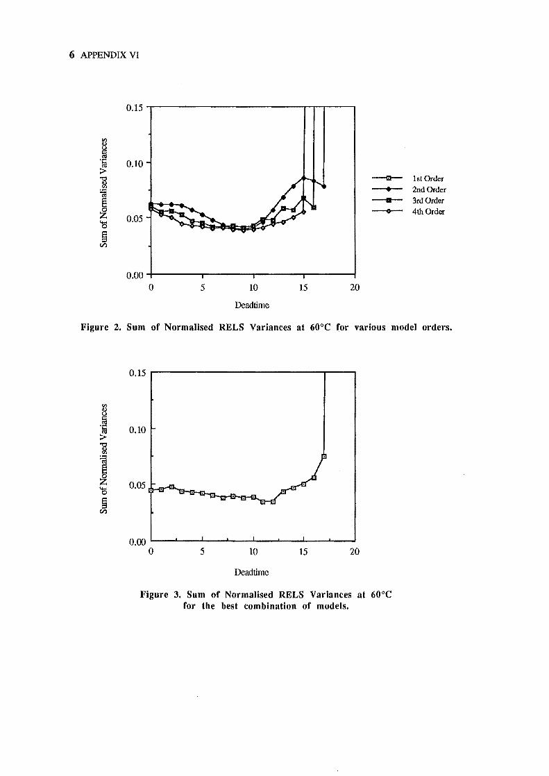
6 APPENDIX VI
0.15 ,-------------,...,-...,.----,
til
8 .! 0.10 :> ~
--a- 1st Order
~ • 2nd Order
~ a 3rdOrder ~ 4th Order
'Cl 0.05
§ V)
0.00 +------,..-----r----r-------/ o 5 10 15 20
Deadtime
Figure 2. Sum of Normalised RELS Variances at 60°C for various model orders.
0.15
til
8 .! :>
0.10
~
1 Z 0.05 'Cl . §
V)
0.00 0 5 10 15 20
Deadtime
Figure 3. Sum of Normalised RELS Variances at 60°C for the best combination of models.
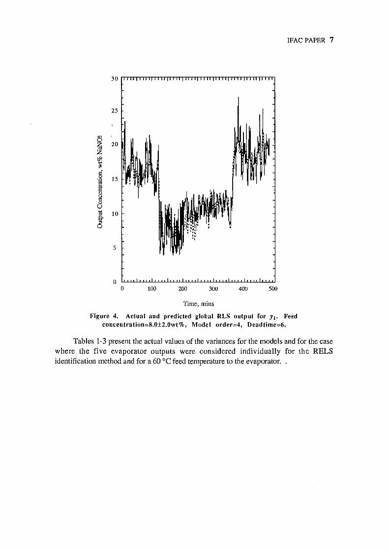
IFAC PAPER 7
a ~
20
~ .... ~
§ '::I
i 15
c 0 u t:i 10 g
5
o 100 200 300 400 500
Time, mins
Figure 4. Actual and predicted global RLS output for Y1' Feed concentration=8.0±2.0wt%, Model order=4, Deadtime=6.
Tables 1-3 present the actual values of the variances for the models and for the case where the five evaporator outputs were considered individually for the RELS identification method and for a 60°C feed temperature to the evaporator. .
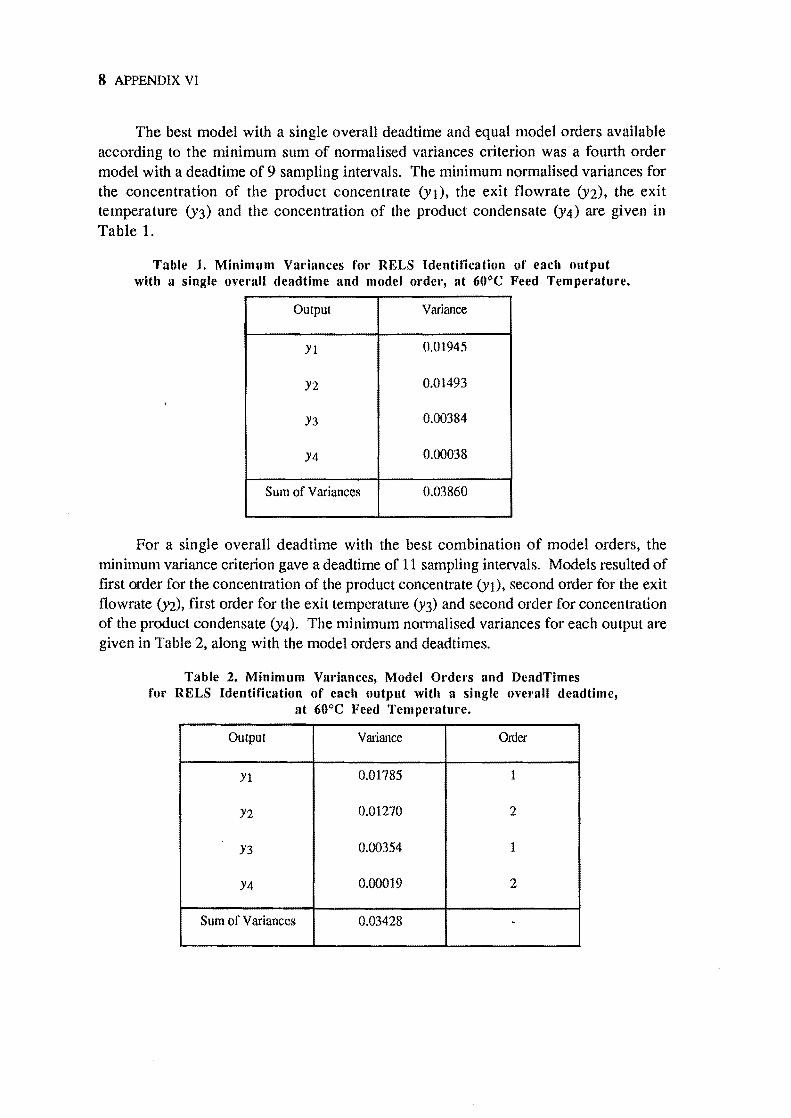
8 APPENDIX VI
The best model with a single overall deadtime and equal model orders available according to the minimum sum of normalised variances criterion was a fourth order model with a dead time of 9 sampling intervals. The minimum normalised variances for the concentration of the product concentrate (Yl). the exit flowrate (Y2), the exit temperature (Y3) and the concentration of the product condensate (Y4) are given in Table 1.
Table 1. Minimum Variances for RELS Identification of each output with a single overall deadtime and model order, at 60°C Feed Temperature.
Output Variance
Yl 0.01945
Y2 0.01493
Y3 0.00384
Y4 0.00038
Sum of Variances 0.03860
For a single overall dead time with the best combination of model orders, the minimum variance criterion gave a deadtime of 11 sampling intervals. Models resulted of first order for the concentration of the product concentrate (YI), second order for the exit fIowrate ()12), first order for the exit temperature (Y3) and second order for concentration of the product condensate (Y4). The minimum normalised variances for each output are given in Table 2, along with the model orders and deadtimes.
Table 2. Minimum Variances, Model Orders and DeadTimes for RELS Identification of each output with a single overall dead time,
at 60°C Feed Temperature.
Output Variance Order
Yl 0.01785 I
Y2 0.01270 2
Y3 0.00354 1
Y4 0.00019 2
Sum of Variances 0.03428 -
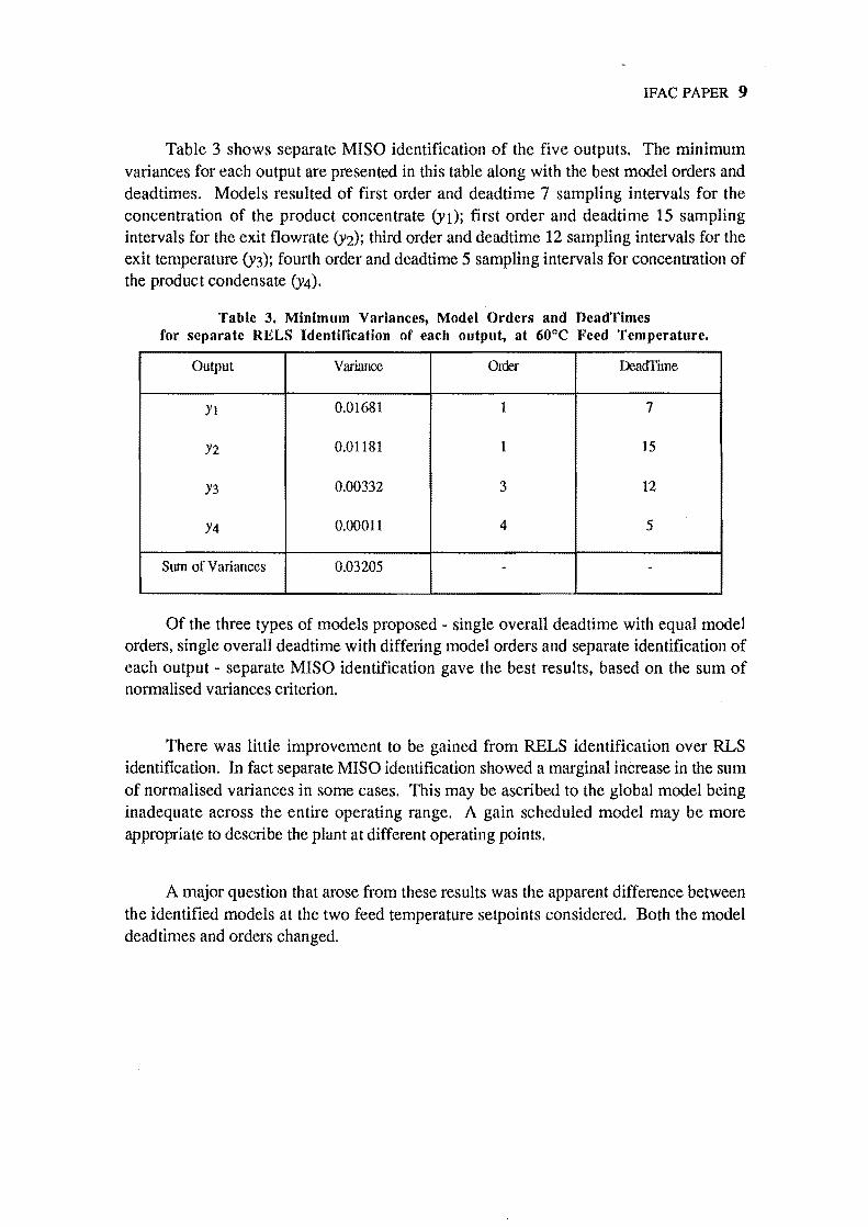
IFAC PAPER 9
Table 3 shows separate MISO identification of the five outputs. The minimum variances for each output are presented in this table along with the best model orders and deadtimes. Models resulted of first order and deadtime 7 sampling intervals for the concentration of the product concentrate (Yl); first order and deadtime 15 sampling intervals for the exit flowrate (Y2); third order and deadtime 12 sampling intervals for the exit temperature (Y3); fourth order and deadtime 5 sampling intervals for concentration of the product condensate (Y4).
Table 3. Minimum Variances, Model Orders and DeadTimes for separate RELS Identification of each output, at 60°C Feed Temperature.
Output Variance Om Dea<ITime
Yl 0.01681 1 7
Y2 0.Q1181 1 15
Y3 0.00332 3 12
Y4 0.00011 4 5
Sum of Variances 0.03205 - -
Of the three types of models proposed - single overall deadtime with equal model orders, single overall deadtime with differing model orders and separate identification of each output - separate MISO identification gave the best results, based on the sum of normalised variances criterion.
There was little improvement to be gained from RELS identification over RLS identification. In fact separate MISO identification showed a marginal increase in the sum of normalised variances in some cases. This may be ascribed to the global model being inadequate across the entire operating range. A gain scheduled model may be more appropriate to describe the plant at different operating points.
A major question that arose from these results was the apparent difference between the identified models at the two feed temperature setpoints considered. Both the model deadtimes and orders changed.
10 APPENDIX VI
The answer to this question may be that a different mechanism operated at each temperature. At 20°C the feed entered the evaporator tube considerably below the boiling point of the liquid in the tube - at least 40 °C below the boiling point at the vacuum pressure used. A large sensible heating region existed where the liquid feed was heated up to the boiling point. At a feed temperature of 60°C the feed entered the evaporator tube at just below the boiling point, so the sensible heating region was much shorter. The time constants and deadtimes of the process must be different. If the evaporator tube is regarded as a small tank filled with liquid, the volume and height of this tank has effectively changed. This change in the tank dynamics was reflected by a change in the identified parameters.
2.2. Gain-scheduled models
The gain scheduling approach is a method used for systems whose parameters change with time. The use of this technique in control may be considered as a form of adaptive control where the parameters of the controller are altered according to some model to follow the variation in process parameters with a change in the plant operating point. Originally this approach was used only to account for change in process gains.
The major drawback of gain scheduling is that it is an open-loop compensation for change in process parameters. The gain schedule must be designed before applying the controller to the process. There is no feedback to compensate for incorrect schedules. The advantage of gain scheduling is that the regulator parameters can be changed quickly in response to process parameter variations.
The least squares methods can also be used directly in the application of a selftuning regulator to systems where the parameters vary with time. For the recursive methods in this setting, the choice of the forgetting factor II., is important, (Goodwin and Sin, 1984). A constant value of 0.98 is often used. The aim is to maximise the tracking effectiveness of the parameter estimation, while minimising the noise sensitivity of the parameter estimates.
The model parameters were re-identified for the model structures found by global identification in the previous section for the two feed temperatures of 20°C and 60 °C and the two input concentration ranges of 2.5±2.0 wt% NaN03 and 8.0±2.0 wt% NaN03. The resultant sums of the model variances can be compared directly with the variances of the global model identifications.
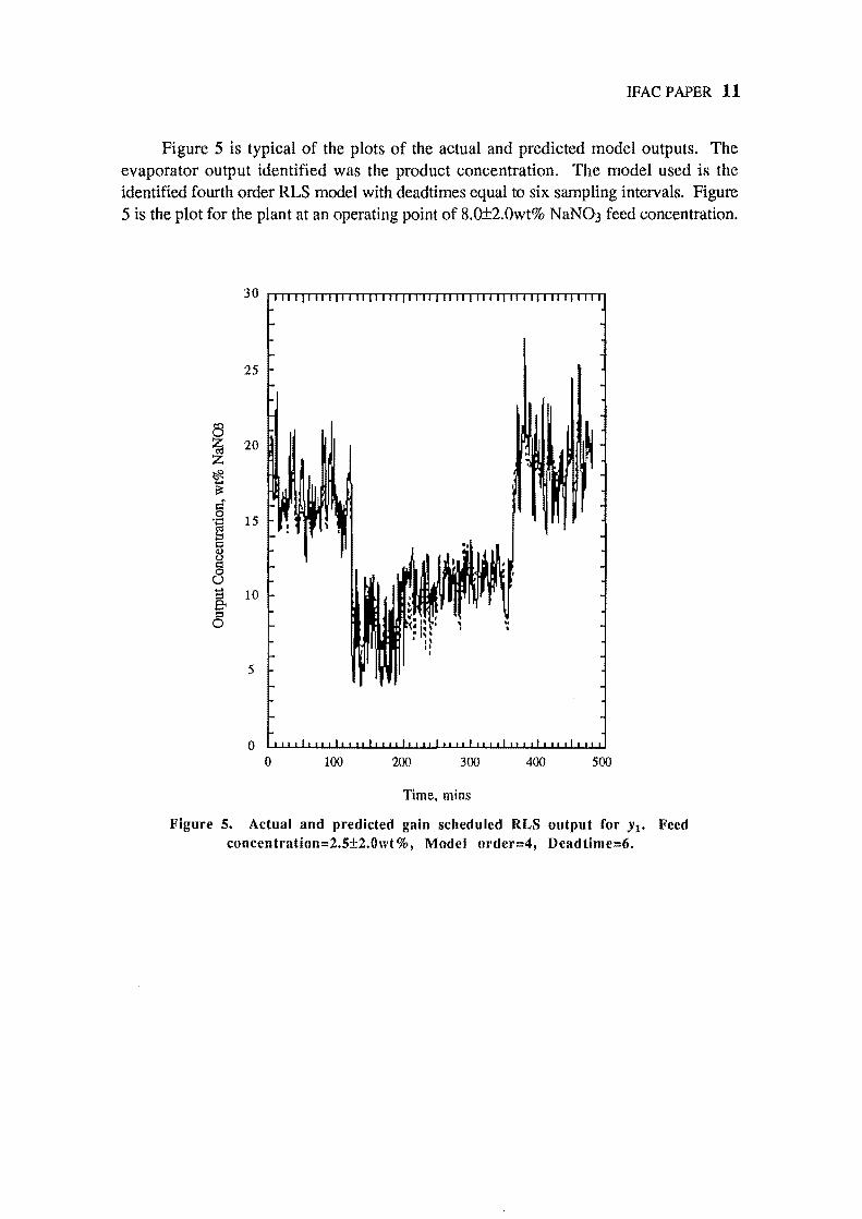
IFAC PAPER 11
Figure 5 is typical of the plots of the actual and predicted model outputs. The evaporator output identified was the product concentration. The model used is the identified fourth order RLS model with deadtimes equal to six sampling intervals. Figure 5 is the plot for the plant at an operating point of 8.o±2.0wt% NaN03 feed concentration.
i 20 Z ~ .... i't d' 0
15 '.0 g @ § u ... 10 ~ g. ~
0 .. . 5
o o 100 200 300 400 500
Time, mins
Figure 5. Actual and predicted gain scheduled RLS output ror Yl' Feed concentration=2.5±2.0wt%, Model order=4, Deadtime=6.
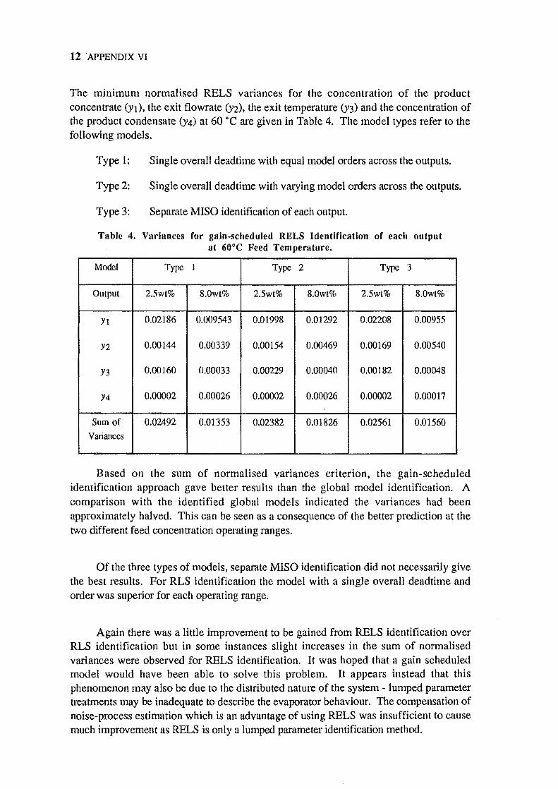
12 'APPENDIX VI
The minimum normalised RELS variances for the concentration of the product concentrate (Yl), the exit flowrate (Y2), the exit temperature (Y3) and the concentration of the product condensate (Y4) at 60 ·C are given in Table 4. The model types refer to the following models.
Type 1: Single overall deadtime with equal model orders across the outputs.
Type 2: Single overall deadtime with varying model orders across the outputs.
Type 3: Separate MISO identification of each output.
Table 4. Variances for gain-scheduled RELS Identification of each output at 60°C Feed Temperature.
Model Type 1 Type 2 Type 3
Output 2.5wt% 8.0wt% 2.5wt% 8.0wt% 2.5wt% 8.0wt%·
Yl 0.02186 0.009543 0.01998 0.01292 0.02208 0.00955
Y2 0.00144 0.00339 0.00154 0.00469 0.00169 0.00540
Y3 0.00160 0.00033 0.00229 0.00040 0.00182 0.00048
Y4 0.00002 0.00026 0.00002 0.00026 0.00002 0.00017
Sum of 0.02492 0.01353 0.02382 0.01826 0.02561 0.01560
Variances
Based on the sum of normalised variances criterion, the gain-scheduled identification approach gave better results than the global model identification. A comparison with the identified global models indicated the variances had been approximately halved. This can be seen as a consequence of the better prediction at the two different feed concentration operating ranges.
Of the three types of models, separate MISO identification did not necessarily give the best results. For RLS identification the model with a single overall deadtime and order was superior for each operating range.
Again there was a little improvement to be gained from RELS identification over RLS identification but in some instances slight increases in the sum of normalised variances were observed for RELS identification. It was hoped that a gain scheduled model would have been able to solve this problem. It appears instead that this phenomenon may also be due to the distributed nature of the system - lumped parameter treatments may be inadequate to describe the evaporator behaviour. The compensation of noise-process estimation which is an advantage of using RELS was insufficient to cause much improvement as RELS is only a lumped parameter identification method.
IFAC PAPER 13
3. DISTRIBUTED PARAMETER MODELS
Deterministic quasi-linear distributed parameter models of the climbing film evaporator may be derived by simply using the measured evaporator variables directly in a simple hyperbolic partial differential equation. The following hyperbolic equations were used.
fl.tL j}n at + a Jz + bl1Yl + bl2Y2 + bnY3 = 0
~ ~ at + a Jz + b2lYl + b22Y2 + b23Y3 = 0
where Yl is concentration of the product concentrate, Y2 is the exit flowrate of the product concentrate and Y3 is the temperature of the product concentrate, a is the characteristc and B is a matrix of parameters.
These equations each have the characteristic equation
dz dt =a
The characteristic a may be approximated by the equation
a= pAHI
where p is the liquid density, A is the flow cross-scetional area and HI is the fractional liquid holdup.
By substituting measured values, the dead time of the analogous lumped parameter system may be calculated in the following manner. Typical values of the variables concerned were used in the calculation.
14 APPENDIX VI
The flow velocity for a feed rate of 0.38 kg/min was
u 1000 kg/min X (1
= 0.690 m/min
The characteristic for this flow velocity was given by
u 0.690 2 3 m/ . a = HI = (f.3 =. mln.
The deadtime value for the corresponding lumped parameter system was then
L 3.0 m 13' 6 7 1" 1 'rd = - = 2 3 / . = . mm = to samp mg mterva s a . m mIn
For a feedrate of 0.17 kg/min, the flow velocity was 0.309 m/min and the characteristic was 1.0 rn/min. The dead time of the "equivalent" lumped parameter system was 2.9 min, which corresponded to 14 to 15 sampling intervals.
The deadtime varies with the feedrate, due to the velocity dependence of the characteristic. This illustrates the point that a single lumped parameter model was inadequate to describe the system. The model parameters varied with operating conditions.
Vetterling et aI., (1986), presents various optimisation routines to solve this identification problem - the Levenberg-Marquardt non-linear least squares method and the Fletcher-Reeves or Poliak-Ribiere algorithms for gradient-based optimisation were suitable. The methods required adaptation so that they may be used to identify the MIMO model of the evaporator.
It was necessary to solve the matrix exponential, e-Bt, as the method of characteristics predicted
where Td is the deadtime of the corresponding lumped parameter system
IFAC PAPER 15
i.e. the characteristic dz dt == a
was approximated as
where L is the length of the evaporator tube.
To obtain a solution it was necessary to concentrate on only one model variable, with the other variables considered as forcing inputs to the system, resulting in the solution of an inhomogeneous equation by the method of characteristics.
fIJ == B'.y(t.z) + C·yfit)
where [
0 C12 C13] C = C21 0 C23
c31 c32 0
and yfit) = y(t,O)
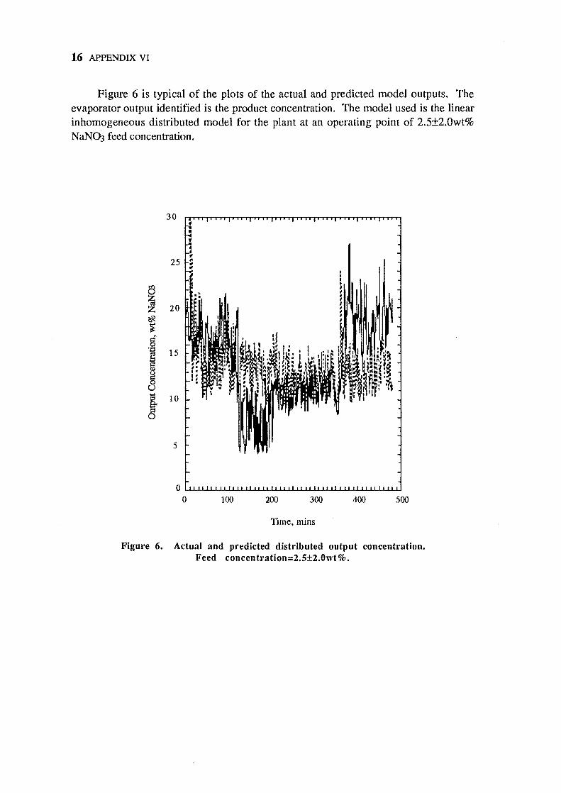
16 APPENDIX VI
Figure 6 is typical of the plots of the actual and predicted model outputs. The evaporator output identified is the product concentration. The model used is the linear inhomogeneous distributed model for the plant at an operating point of 2.5±2.0wt% NaN~ feed concentration.
30
25
8 ~ 20 ~ ~
.~ ~
15
g 0 u ::J 10 ~ 0
5
o ~~~~~~~~~~~~~~~~~~ o 100 200 300 400 500
Time. mins
Figure 6. Actual and predicted distl'ibuted output concentration. Feed concentration=2.S±2.0wt %.
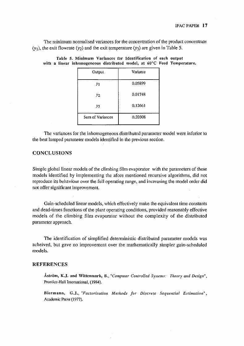
IFACPAPER 17
The minimum normalised variances for the concentration of the product concentrate (Yl), the exit flowrate (Y2) and the exit temperature (Y3) are given in Table 5.
Table 5. Minimum Variances for Identification of each output with a linear inhomogeneous distributed model, at 60"C Feed Temperature.
Output Variance
Yl 0.05899
Y2 0.01748
Y3 0.12661
Sum of Variances 0.20308
The variances for the inhomogeneous distributed parameter model were inferior to the best lumped parameter models identified in the previous section.
CONCLUSIONS
Simple global linear models of the climbing film evaporator with the parameters of these models identified by implementing the afore mentioned recursive algorithms, did not reproduce its behaviour over the full operating range, and increasing the model order did not offer significant improvement.
Gain-scheduled linear models, which effectively make the equivalent time constants and dead-times functions of the plant operating conditions, provided reasonably effective models of the climbing film evaporator without the complexity of the distributed parameter approach.
The identification of simplified deterministic distributed parameter models was acheived, but gave no improvement over the mathematically simpler gain-scheduled models.
REFERENCES
Astrom, K.J. and Wittenmark, B., "Computer Controlled Systems: Theory and Design",
Prentice-Hall International, (1984),
Biermann, G.J., "Factorisation Methods for Discrete Sequential Estimation",
Academic Press (1977).
18 APPENDIX VI
Carpenter, W.T., Wozny, M.J. and Goodson, R.E., "Distributed Parameter
Identification Using the Method of Characteristics", Trans. ASME, J. Dynamic Systems,
Measurement and Control, Vol. 93, (1971).
Crawford, R.A. and Austin, P.C., "Control of an Evaporator", Proc. 3rd Int. Symp. on
Process Systems Engineering, Sydney, Australia (1988).
Goodwin, G.C. and Sin, K.S., "Adaptive filtering prediction and control",
Prentice-Hall (1984).
Isermann, R., "Comparison and Evaluation of 6 On-line Identification and Parameter
Estimation Methods with 3 Simulated Processes", Proc. Symp. on Identification and Parameter
Estimation, The Hague/Delft, The Netherlands, Pergamon Press (1973).
Kubrusly, C.S., "Distributed parameter system identification. A survey", Int. J. Control,
Vo1.26, No.4 (1977).
Ljung, L., "System Identification - Theory for the User", Prentice-Hall (1987).
Ljung, L. and Soderstrom, T., "Theory and Practice of Recursive Identification",
MIT Press (1983).
Montgomery, D.C., "Design and Analysis of Experiments", 2nd Ed., Wiley (1984).
Polis, M.P., "The Distributed System Parameter Identification Problem: A Survey of Recent
Results", Proc. 3rd IFAC Symp. on Control of Distributed Parameter Systems, Tolouse, France
(1982).
Polis, M.P. and Goodson, R.E., "Parameter Identification in Distributed Parameter
Systems: A Sythesizing Overview", Proc. IEEE, Vol. 64. No.1 (1976).
Ray, W.H •• "Some Recent Applications of Distributed Parameter Systems Theory - A Survey".
Automatica, Vol.14 (1978).
Soderstrom, T. and Stoica, P., "System Identification", Prentice-Hall (1989),
Vetterling, W.T., Teukolsky, S.A., Press, W.H. and Flannery, B.P., "Numerical
Recipes", Cambridge University Press. (1986).