Embed Size (px)
Citation preview
INTERNATIONAL JOURNAL FOR NUMERICAL METHODS IN ENGINEERINGInt. J. Numer. Meth. Engng 2008; 76:1328–1352Published online 19 June 2008 in Wiley InterScience (www.interscience.wiley.com). DOI: 10.1002/nme.2353
Modeling three-dimensional crack propagation—A comparisonof crack path tracking strategies
P. Jager1, P. Steinmann2 and E. Kuhl3,∗,†
1Department of Mechanical Engineering, University of Kaiserslautern, 67653 Kaiserslautern, Germany2Department of Mechanical Engineering, Friedrich-Alexander University Erlangen-Nuremberg,
91058 Erlangen, Germany3Department of Mechanical Engineering, Stanford University, Stanford, CA-94305, U.S.A.
SUMMARY
The development of a new finite element technique for the simulation of discontinuous failure phenomenain three dimensions is the key objective of this study. In contrast to the widely used extended finiteelement technique, we apply a purely deformation-based strategy based on an independent interpolationof the deformation field on both sides of the discontinuity. This method has been applied successfully fortwo-dimensional crack propagation problems in the past. However, when it comes to three-dimensionalfailure phenomena, it faces the same difficulties as the extended finite element method. Unlike in twodimensions, the characterization for the three-dimensional failure surface is non-unique and the trackingof the discrete crack can be performed in several conceptually different ways. In this work, we reviewthe four most common three-dimensional crack tracking strategies. We perform a systematic comparisonin terms of standard algorithmic quality measures such as mesh independency, efficiency, robustness,stability and computational cost. Moreover, we discuss more specific issues such as crack path continuityand integratability in commercial finite element packages. The features of the suggested crack trackingalgorithms will be elaborated by means of characteristic benchmark problems in failure analysis. Copyrightq 2008 John Wiley & Sons, Ltd.
Received 17 September 2007; Revised 24 February 2008; Accepted 25 February 2008
KEY WORDS: three-dimensional crack propagation; fixed tracking; local tracking; global tracking;cohesive zone model; discrete failure
∗Correspondence to: E. Kuhl, Department of Mechanical Engineering, Stanford University, Stanford, CA 94305-4040,U.S.A.
†E-mail: [email protected]
Contract/grant sponsor: German National Science Foundation
Copyright q 2008 John Wiley & Sons, Ltd.
MODELING THREE-DIMENSIONAL CRACK PROPAGATION 1329
1. MOTIVATION
The reliable prediction of crack propagation and failure of brittle materials and structures is anintegral part in material design and structural analysis. In order to predict not only the failureload but also the post-peak behavior correctly, robust and stable computational algorithms thatare capable of dealing with the highly non-linear set of governing equations are an essentialrequirement. Traditionally, finite element methods have been applied to model material failure ina smeared sense, i.e. continuous smooth failure was attributed to a softening stress–strain curvein the form of plasticity or damage on the element level. Discrete failure, however, was ratherattributed to predefined interfaces that had to be introduced a priori as potential failure surfacesat selected inter-element boundaries. According to the cohesive zone concept, discrete failure wasthen collectively lumped into softening traction separation laws within the interface element.
The first method to truly simulate arbitrary discrete failure surfaces was the embedded disconti-nuity technique, see [1–6]. Motivated by the assumed enhanced strain concept, additional degreesof freedom were introduced locally on the element level to characterize the failure plane. Theembedded discontinuity technique convinced through its computational efficiency: Due to thelocal nature of the enhancement, the size of the global system of equations was not effectedby the newly introduced failure surface. An obvious drawback of the local crack representation,however, was the discontinuous nature of the failure surface that was soon found to introduce stresslocking associated with an over-estimation of the structural stiffness. To overcome this deficiency,Belytschko and co-workers [7, 8] introduced a technique to successfully capture smooth failuresurfaces: the celebrated extended finite element method. At the additional cost of successivelyintroducing additional global degrees of freedom, smooth discrete cracks could finally be modeledanywhere in the domain, see also [9–13]. While Belytschko’s extended finite element methoduses the displacement jump as additional unknown, Hansbo’s method advocated herein worksexclusively with deformation degrees of freedom, see [14–19]. Based on a re-parameterization ofunknowns, the latter shows certain advantages in combination with particular structural elementssuch as shells, see Areias and Belytschko [20], Areias et al. [21] or Jager et al. [22].
For two-dimensional problems, both Belytschko’s extended finite element method and Hansbo’smethod soon became popular to model concrete failure and brittle failure of composites, see[7–18, 22, 23]. In a two-dimensional setting, the tracking of crack propagation is rather straightfor-ward. Once an element is identified to fail, typically decided based on a maximum principal stresscriterion, the crack extends from a neighboring crack point on the element edge in the directionnormal to the maximum principal stress. Although this stress-based crack propagation criterionalways renders a unique and smooth C0-continuous failure zone in two-dimensional analyses, iteventually yields a non-smooth failure surface in a three-dimensional setting. Recent attempts inthe literature have addressed the issue of crack propagation in three-dimensional failure analysisand a number of different strategies have been presented, see, e.g. [19, 22, 24–39]. This articleaddresses four of the most common approaches to track three-dimensional crack propagation andcompares their algorithmic realization by means of common quality measures such as robustness,stability, efficiency, computational cost, mesh objectivity, generality and crack surface continuity.
The algorithm we discuss first is the fixed crack tracking scheme for which, similar to computa-tions based on classical interface elements, the crack path has to be a priori known. This algorithmis thus pretty simple and boils down to deciding whether the stresses in the next element ofthe potential crack path exceed the critical failure stress and the element fails or rather remainscontinuous. From a computational point of view, this algorithm is particularly robust and stable.
Copyright q 2008 John Wiley & Sons, Ltd. Int. J. Numer. Meth. Engng 2008; 76:1328–1352DOI: 10.1002/nme
1330 P. JAGER, P. STEINMANN AND E. KUHL
A slightly more complicated scheme is the local crack tracking scheme, which can be interpretedas the three-dimensional generalization of crack tracking in two-dimensional failure analysis. Here,the crack essentially extends from neighboring crack points and proceeds in the direction normalto the maximum principal stress. As this concept would eventually render non-smooth surfaces,Areias and Belytschko [24] have suggested to adjust the crack plane normal based on neighboringcrack intersection points. In the case of too many neighboring points, however, the system isover-determined and the crack hardly deviates from a planar surface. The structural stiffness mightthus be severely overestimated.
A non-local crack tracking scheme is a successful means to remedy this deficiency. By averagingthe crack plane normal over a certain neighborhood, Gasser and Holzapfel [27, 28] ensure thatthe generated failure surface is smooth in average, see also [29, 40]. However, as for all non-localaveraging techniques, this concept is not really tailored to the modular element-wise nature offinite element analyses. Although theoretically elegant, it is rather cumbersome to include it intoexisting finite element codes as it affects not only the integration point and the element level butalso the global structural level.
An extremely elegant and yet very powerful strategy that circumvents nearly all of the defi-ciencies above is the global crack tracking scheme introduced recently by Oliver and co-workers[25, 34, 41]. It provides a finite element-specific solution to the problem of kinematic crack char-acterization as it introduces an additional scalar-valued unknown that defines one or multiplecrack surfaces as isosurfaces of this additional field of unknowns, see [26, 29, 42, 43]. Contin-uous smooth, planar or curved discontinuity surfaces can thus be described in a robust and stablemanner, however, at the cost of having to solve an additional global system of equations withinthe post-processing step. Global crack tracking is not only by far the most general of all the fourstrategies, due to its modular nature, it can also be incorporated into existing finite element codesin an efficient and straightforward way.
In this article, we would like to share our experience and some of the sneaky tricks to success-fully model crack propagation in three-dimensional domains. This article is organized as follows.Section 2 briefly summarizes the governing equations of a continuous body crossed by a discon-tinuity surface. In addition, it illustrates their finite element discretization based on a purelydeformation-based Hansbo interpolation scheme. Sections 3–6 are organized in the same manner.They first introduce the algorithm of the individual crack tracking scheme and then provide anillustrative example. Section 3 discusses fixed crack tracking for which the potential failure surfacehas to be a priori known. Section 4 summarizes local crack tracking, which is a straightforwardgeneralization of the algorithms typically applied in two-dimensional problems. Section 5 intro-duces non-local crack tracking based on a particular spatial averaging technique for the crackplane normal. Section 6 discusses global crack tracking based on solving an additional globalsystem of equations defining the smooth and continuous crack surface. Section 8 then concludeswith a critical discussion of all four schemes. Based on a systematic comparison, we try to givefinal advice and summarize which of the methods would be superior for particular subclasses ofthree-dimensional crack propagation phenomena.
2. SIMULATION OF CRACK PROPAGATION
To introduce the basic notation, we briefly discuss the governing equations for a continuous bodyB crossed by a discontinuity �. For this type of problems, it proves convenient to introduce two
Copyright q 2008 John Wiley & Sons, Ltd. Int. J. Numer. Meth. Engng 2008; 76:1328–1352DOI: 10.1002/nme

MODELING THREE-DIMENSIONAL CRACK PROPAGATION 1331
sets of equations, i.e. two kinematic, equilibrium and constitutive equations, one for the continuousbody B and one for the discontinuity surface � itself. These will be summarized in the sequel.
2.1. Kinematic equations
To ensure uniqueness of the kinematic description, the non-linear deformation u mapping particlesfrom their original position X in the reference configuration B to their current position x in thedeformed configuration S is introduced independently on both sides of the discontinuity, B+ andB−, see Figure 1
u(X) :={u+(X)
u−(X), F=
{F+ =∇Xu
+ ∀X∈B+
F− =∇Xu− ∀X∈B− (1)
Accordingly, we can introduce independent deformation gradients F+ and F− and correspondingJacobians J+=det(F+) and J− =det(F−) on either side of the discontinuity. This parameteriza-tion inherently captures jumps �u� in the deformation map, which obviously take the followingstraightforward representation �u�=u+−u− ∀X∈�.
As illustrated in Figure 2, all particles initially located on the unique discontinuity surface �are mapped onto two surfaces �+ and �− in the deformed configuration. To uniquely characterizediscontinuous failure at finite deformations, we apply the concept of a fictitious discontinuity u,which is assumed to be located right between the two discontinuity surfaces �+ and �− in thedeformed configuration
u := 12 [u++u−], F= 1
2 [F++F−] ∀X∈� (2)
Figure 1. Kinematics—Independent mappings u+ and u− on both sides B+ and B− of the discontinuity� inherently introducing jump ��� in the deformation field.
Figure 2. Kinematics—Concept of fictitious discontinuity surface � located between the twodiscontinuity surfaces �+ and �−.
Copyright q 2008 John Wiley & Sons, Ltd. Int. J. Numer. Meth. Engng 2008; 76:1328–1352DOI: 10.1002/nme
1332 P. JAGER, P. STEINMANN AND E. KUHL
Again, the corresponding deformation gradient F and its Jacobian J =det F follow straightfor-wardly. The normal n to the fictitious discontinuity that will essentially be needed to determinenormal and shear resultants on the discontinuity � can then be expressed through the classicalNanson formula as n= J F−t ·N.
2.2. Equilibrium equations
In the absence of body forces and inertia terms, the equilibrium of external and internal forcesrequires that the divergence of the Piola stress P with respect to the reference configuration vanishesidentically in both subdomains B+ and B−
Div(P)=0 ∀X∈B+∪B− (3)
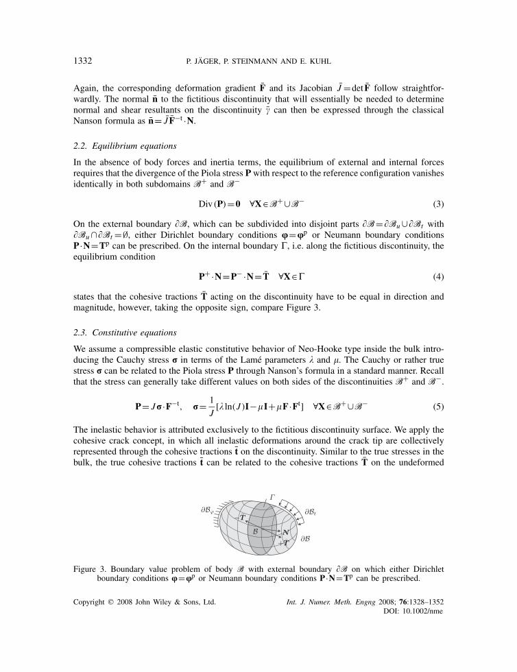
On the external boundary �B, which can be subdivided into disjoint parts �B=�Bu∪�Bt with�Bu∩�Bt =∅, either Dirichlet boundary conditions u=up or Neumann boundary conditionsP ·N=Tp can be prescribed. On the internal boundary �, i.e. along the fictitious discontinuity, theequilibrium condition
P+ ·N=P− ·N= T ∀X∈� (4)
states that the cohesive tractions T acting on the discontinuity have to be equal in direction andmagnitude, however, taking the opposite sign, compare Figure 3.
2.3. Constitutive equations
We assume a compressible elastic constitutive behavior of Neo-Hooke type inside the bulk intro-ducing the Cauchy stress r in terms of the Lame parameters � and �. The Cauchy or rather truestress r can be related to the Piola stress P through Nanson’s formula in a standard manner. Recallthat the stress can generally take different values on both sides of the discontinuities B+ and B−.
P= Jr·F−t, r= 1
J[� ln(J )I−�I+�F ·Ft] ∀X∈B+∪B− (5)
The inelastic behavior is attributed exclusively to the fictitious discontinuity surface. We apply thecohesive crack concept, in which all inelastic deformations around the crack tip are collectivelyrepresented through the cohesive tractions t on the discontinuity. Similar to the true stresses in thebulk, the true cohesive tractions t can be related to the cohesive tractions T on the undeformed
Figure 3. Boundary value problem of body B with external boundary �B on which either Dirichletboundary conditions u=up or Neumann boundary conditions P ·N=Tp can be prescribed.
Copyright q 2008 John Wiley & Sons, Ltd. Int. J. Numer. Meth. Engng 2008; 76:1328–1352DOI: 10.1002/nme
MODELING THREE-DIMENSIONAL CRACK PROPAGATION 1333
domain through Nanson’s formula in terms of area elements da and dA. We conveniently assumea decoupling of the normal and tangential constitutive behavior and introduce the true or ratherCauchy tractions t in the following form:
T= da
dAt, t= fn exp
(− fnGn
�u�· n)n+Et [I− n⊗ n]·�u� ∀X∈� (6)
In the normal direction, fn and Gn denote the tensile strength and the fracture energy, respectively.In the tangential direction, Et denotes the shear stiffness.
2.4. Weak form
After multiplication with the corresponding test functions �u and ��u�, integration over the domainof interest, and inclusion of the Neumann boundary conditions, the equilibrium equations (3) and(4) render the weak form∫
B+∪B−�F :PdV +
∫�
��u�·TdA=∫
�Bt
�u ·Tp dA (7)
which essentially constitutes the basis for the finite element discretization to be discussed in thesequel.
2.5. Discretization
For the finite element formulation, it proves convenient to distinguish between standard contin-uous elements and discontinuous elements that are crossed by the discontinuity surface. For thecontinuous elements, we apply a standard interpolation of the test functions �u, the deformationfield u, and their gradients �F and F
�u =nen∑i=1
�ui Ni , u =
nen∑j=1u j N
j
�F =nen∑i=1
�ui ⊗∇XNi , F =
nen∑j=1u j ⊗∇XN
j
∀X∈B (8)
Here Ni and N j are the standard shape functions for tetrahedral elements and nen is the numberof element nodes. For the discontinuous elements, we apply an independent interpolation ofthe deformation fields u+ and u− and its gradients F+ and F− on the individual sides of thediscontinuities B+ and B−. Conceptually speaking, both deformation fields u+ and u− areinterpolated over the entire element through the nodal values in terms of the standard basisfunctions Ni . To this end, double the degrees of freedom and introduce two sets of standard shapefunctions with n+
en nodes for the interpolation on one side of the discontinuity and n−en nodes
for the other side. The interpolated fields are then set to zero on one side of the discontinuity,while they take their usual values on the other side. The jumps in the test function ��u�=∑n+
eni=1 �u+
i Ni −∑n−
eni=1 �u−
i Ni and in the displacement field �u�=∑n+
enj=1u
+j N
j −∑n−enj=1u
−j N
j canthen be expressed as the difference of the two continuous fields evaluated at the internal boundary �.
The average deformation gradient on the fictitious discontinuity surface F= 12 [∑n+
enj=1u
+j ⊗∇XN j +
Copyright q 2008 John Wiley & Sons, Ltd. Int. J. Numer. Meth. Engng 2008; 76:1328–1352DOI: 10.1002/nme
1334 P. JAGER, P. STEINMANN AND E. KUHL
∑n−enj=1u
−j ⊗∇XN j ] follows accordingly
��u� =n+en+n−
en∑i=1
�ui Ni , �u� =
n+en+n−
en∑j=1
u j Nj
�F =n+en+n−
en∑i=1
�ui ⊗∇X Ni , F =
n+en+n−
en∑j=1
u j ⊗∇X Nj
∀X∈� (9)
To unify the notation, we have rearranged the terms in the interpolation and introduced the set Nwhich consists of the element shape functions N evaluated at � multiplied by the correspondingalgebraic sign. Accordingly, ∇X N denotes the gradient of the shape functions N evaluated at �,weighted by the factor 1
2 . With the help of the above-introduced discretizations, the weak form ofthe governing equations (7) can be cast into the following discrete residual statement:
RI =nel
Ae=1
∫Be∪B+,−
d
∇XNi ·PdV +
∫�N i T(�u�)d A−
∫�Bte
N i Tp dA.=0 (10)
where the operatorAnel
e=1 denotes the assembly of all element contributions, i.e. the continuous andthe discontinuous ones. The above residual statement is solved numerically by using an incrementaliterative Newton–Raphson scheme. The solution to the underlying linearized system of equationsRk+1I =Rk
I +dRI.=0 with the iterative residual dRI =∑nnp
J=1KI J duJ and the incremental stiffnessmatrix KI J =�RI /�uJ with
KI J =nel
Ae=1
∫Be∪B+,−
d
∇XNi ·[�FP]·∇XN
j dV
+∫
�N i [��u�T]N j + N i [�FT]·∇X N
jd A (11)
renders the incremental update of the vector of unknowns duJ . The terms in brackets, i.e. thesecond-, third- and fourth-order tensors [��u�T], [�FT], [�FP] depend on the choice of the consti-tutive equations for the stresses in the continuous body and for the tractions on the discontinuitysurface. For the particular choice suggested in (5) and (6) they are given, e.g. in Mergheim et al.[19] or Jager et al. [22]. Recall that due to the chosen discretization scheme, the number of globalnode points nnp, which consists of the standard nodes and the additional duplicated node pointsfor the discontinuous elements, increases progressively during ongoing crack propagation.
2.6. Crack propagation
Following the classical principal stress-based Rankine criterion, we allow the crack to propagateif the largest eigenvalue max{��
i } of the Cauchy stress exceeds the critical failure stress �crit andthus ��>0
�� =max{��i }−�crit>0 with r=
3∑i=1
��i n
�i ⊗n�
i (12)
Copyright q 2008 John Wiley & Sons, Ltd. Int. J. Numer. Meth. Engng 2008; 76:1328–1352DOI: 10.1002/nme
MODELING THREE-DIMENSIONAL CRACK PROPAGATION 1335
The related maximum principal stress direction n�(max{��i }) and its pull back to the reference
configuration N� = J−1Ft ·n� will prove essential for the kinematic characterization of the disconti-nuity surface. Unfortunately, unlike in two dimensions, the kinematic description of the propagatingfailure surface is non-unique in the three-dimensional setting. In the following sections, we intro-duce and discuss the four most prominent strategies for tracking failure surfaces and determiningthe crack plane normal Ncrk in three-dimensional crack propagation problems.
Remark 1 (Non-local crack propagation criterion)To avoid spurious crack path oscillations, the Rankine criterion (12) is typically not evalu-ated in terms of the local stress r. Instead a non-local averaging is applied and the eigenvalueproblem is solved for the non-local stress r, see, e.g. Jirasek et al. [44]. In the discrete settingand for constant strain elements, r can simply be calculated as the volume average stress r=∑
j∈I� Vjr j/∑
j∈I� Vj . The volume average stress r is evaluated in all elements within the setI�. This set contains all elements in a sphere of a user-defined radius r� around the currentpotential cracking point.
3. FIXED TRACKING
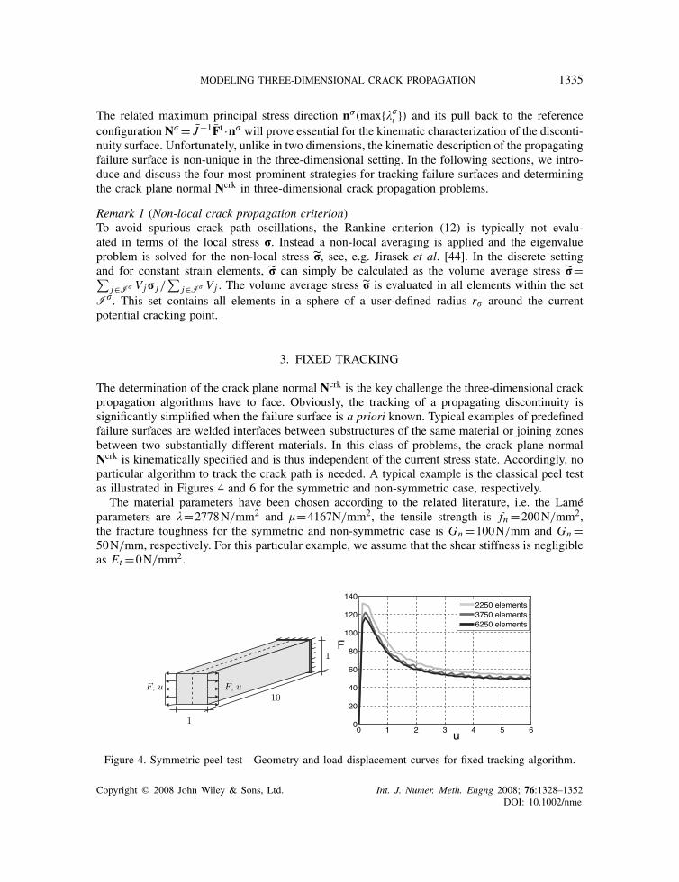
The determination of the crack plane normal Ncrk is the key challenge the three-dimensional crackpropagation algorithms have to face. Obviously, the tracking of a propagating discontinuity issignificantly simplified when the failure surface is a priori known. Typical examples of predefinedfailure surfaces are welded interfaces between substructures of the same material or joining zonesbetween two substantially different materials. In this class of problems, the crack plane normalNcrk is kinematically specified and is thus independent of the current stress state. Accordingly, noparticular algorithm to track the crack path is needed. A typical example is the classical peel testas illustrated in Figures 4 and 6 for the symmetric and non-symmetric case, respectively.
The material parameters have been chosen according to the related literature, i.e. the Lameparameters are �=2778N/mm2 and �=4167N/mm2, the tensile strength is fn =200N/mm2,the fracture toughness for the symmetric and non-symmetric case is Gn =100N/mm and Gn =50N/mm, respectively. For this particular example, we assume that the shear stiffness is negligibleas Et =0N/mm2.
0 1 2 3 4 5 60
20
40
60
80
100
120
140
u
F
2250 elements3750 elements6250 elements
Figure 4. Symmetric peel test—Geometry and load displacement curves for fixed tracking algorithm.
Copyright q 2008 John Wiley & Sons, Ltd. Int. J. Numer. Meth. Engng 2008; 76:1328–1352DOI: 10.1002/nme
1336 P. JAGER, P. STEINMANN AND E. KUHL
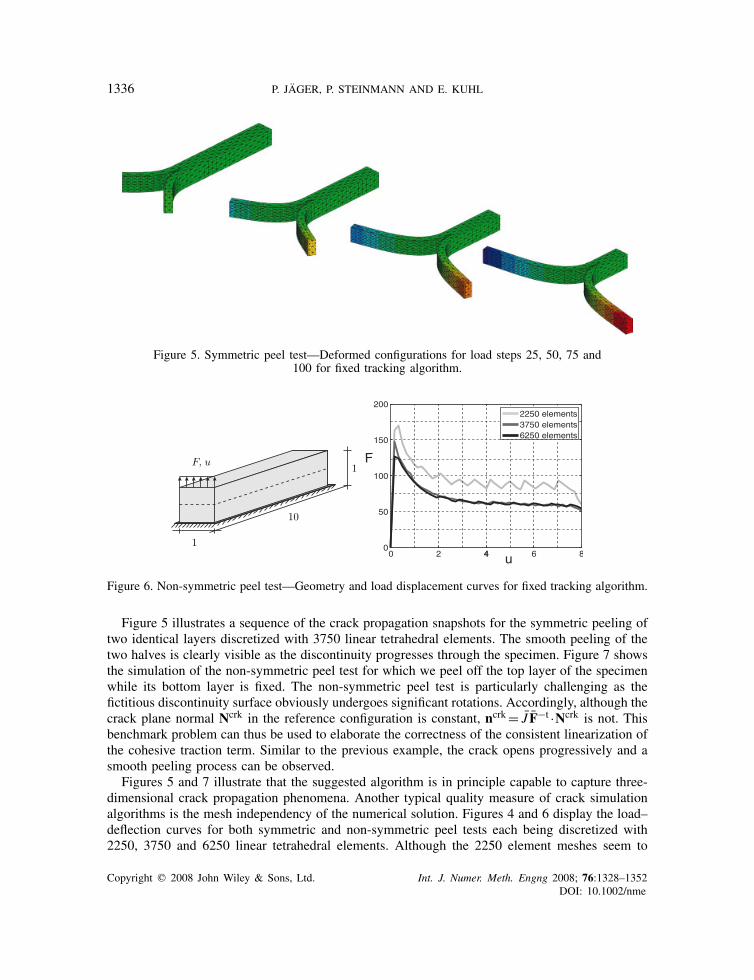
Figure 5. Symmetric peel test—Deformed configurations for load steps 25, 50, 75 and100 for fixed tracking algorithm.
0 2 4 6 80
50
100
150
200
u
F
4
2250 elements3750 elements6250 elements
Figure 6. Non-symmetric peel test—Geometry and load displacement curves for fixed tracking algorithm.
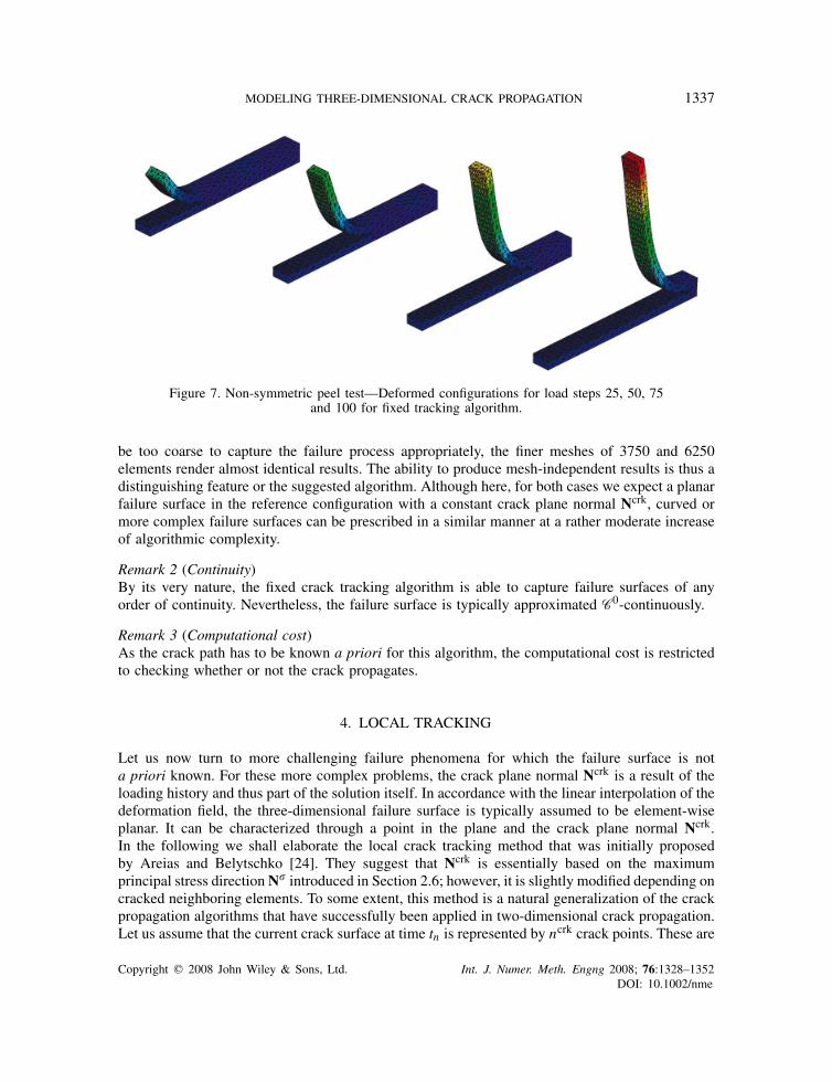
Figure 5 illustrates a sequence of the crack propagation snapshots for the symmetric peeling oftwo identical layers discretized with 3750 linear tetrahedral elements. The smooth peeling of thetwo halves is clearly visible as the discontinuity progresses through the specimen. Figure 7 showsthe simulation of the non-symmetric peel test for which we peel off the top layer of the specimenwhile its bottom layer is fixed. The non-symmetric peel test is particularly challenging as thefictitious discontinuity surface obviously undergoes significant rotations. Accordingly, although thecrack plane normal Ncrk in the reference configuration is constant, ncrk= J F−t ·Ncrk is not. Thisbenchmark problem can thus be used to elaborate the correctness of the consistent linearization ofthe cohesive traction term. Similar to the previous example, the crack opens progressively and asmooth peeling process can be observed.
Figures 5 and 7 illustrate that the suggested algorithm is in principle capable to capture three-dimensional crack propagation phenomena. Another typical quality measure of crack simulationalgorithms is the mesh independency of the numerical solution. Figures 4 and 6 display the load–deflection curves for both symmetric and non-symmetric peel tests each being discretized with2250, 3750 and 6250 linear tetrahedral elements. Although the 2250 element meshes seem to
Copyright q 2008 John Wiley & Sons, Ltd. Int. J. Numer. Meth. Engng 2008; 76:1328–1352DOI: 10.1002/nme
MODELING THREE-DIMENSIONAL CRACK PROPAGATION 1337
Figure 7. Non-symmetric peel test—Deformed configurations for load steps 25, 50, 75and 100 for fixed tracking algorithm.
be too coarse to capture the failure process appropriately, the finer meshes of 3750 and 6250elements render almost identical results. The ability to produce mesh-independent results is thus adistinguishing feature or the suggested algorithm. Although here, for both cases we expect a planarfailure surface in the reference configuration with a constant crack plane normal Ncrk, curved ormore complex failure surfaces can be prescribed in a similar manner at a rather moderate increaseof algorithmic complexity.
Remark 2 (Continuity)By its very nature, the fixed crack tracking algorithm is able to capture failure surfaces of anyorder of continuity. Nevertheless, the failure surface is typically approximated C0-continuously.
Remark 3 (Computational cost)As the crack path has to be known a priori for this algorithm, the computational cost is restrictedto checking whether or not the crack propagates.
4. LOCAL TRACKING
Let us now turn to more challenging failure phenomena for which the failure surface is nota priori known. For these more complex problems, the crack plane normal Ncrk is a result of theloading history and thus part of the solution itself. In accordance with the linear interpolation of thedeformation field, the three-dimensional failure surface is typically assumed to be element-wiseplanar. It can be characterized through a point in the plane and the crack plane normal Ncrk.In the following we shall elaborate the local crack tracking method that was initially proposedby Areias and Belytschko [24]. They suggest that Ncrk is essentially based on the maximumprincipal stress directionN� introduced in Section 2.6; however, it is slightly modified depending oncracked neighboring elements. To some extent, this method is a natural generalization of the crackpropagation algorithms that have successfully been applied in two-dimensional crack propagation.Let us assume that the current crack surface at time tn is represented by ncrk crack points. These are
Copyright q 2008 John Wiley & Sons, Ltd. Int. J. Numer. Meth. Engng 2008; 76:1328–1352DOI: 10.1002/nme
1338 P. JAGER, P. STEINMANN AND E. KUHL
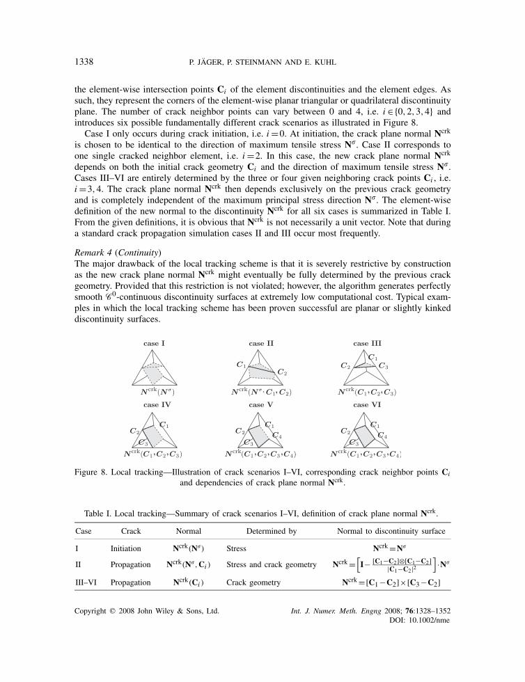
the element-wise intersection points Ci of the element discontinuities and the element edges. Assuch, they represent the corners of the element-wise planar triangular or quadrilateral discontinuityplane. The number of crack neighbor points can vary between 0 and 4, i.e. i ∈{0,2,3,4} andintroduces six possible fundamentally different crack scenarios as illustrated in Figure 8.
Case I only occurs during crack initiation, i.e. i=0. At initiation, the crack plane normal Ncrk
is chosen to be identical to the direction of maximum tensile stress N�. Case II corresponds toone single cracked neighbor element, i.e. i=2. In this case, the new crack plane normal Ncrk
depends on both the initial crack geometry Ci and the direction of maximum tensile stress N�.Cases III–VI are entirely determined by the three or four given neighboring crack points Ci , i.e.i=3,4. The crack plane normal Ncrk then depends exclusively on the previous crack geometryand is completely independent of the maximum principal stress direction N�. The element-wisedefinition of the new normal to the discontinuity Ncrk for all six cases is summarized in Table I.From the given definitions, it is obvious that Ncrk is not necessarily a unit vector. Note that duringa standard crack propagation simulation cases II and III occur most frequently.
Remark 4 (Continuity)The major drawback of the local tracking scheme is that it is severely restrictive by constructionas the new crack plane normal Ncrk might eventually be fully determined by the previous crackgeometry. Provided that this restriction is not violated; however, the algorithm generates perfectlysmooth C0-continuous discontinuity surfaces at extremely low computational cost. Typical exam-ples in which the local tracking scheme has been proven successful are planar or slightly kinkeddiscontinuity surfaces.
Figure 8. Local tracking—Illustration of crack scenarios I–VI, corresponding crack neighbor points Ci
and dependencies of crack plane normal Ncrk.
Table I. Local tracking—Summary of crack scenarios I–VI, definition of crack plane normal Ncrk.
Case Crack Normal Determined by Normal to discontinuity surface
I Initiation Ncrk(N�) Stress Ncrk=N�
II Propagation Ncrk(N�,Ci ) Stress and crack geometry Ncrk=[I− [C1−C2]⊗[C1−C2]
|C1−C2|2]·N�
III–VI Propagation Ncrk(Ci ) Crack geometry Ncrk=[C1−C2]×[C3−C2]
Copyright q 2008 John Wiley & Sons, Ltd. Int. J. Numer. Meth. Engng 2008; 76:1328–1352DOI: 10.1002/nme
MODELING THREE-DIMENSIONAL CRACK PROPAGATION 1339
Remark 5 (Computational cost)Assume that the dynamic list of crack tip elements contains ntip entries. Moreover, each tetrahedralelement has four neighboring elements that are identified and stored in a neighbor list at theinitialization of the mesh. The computational effort of this algorithm is thus remarkably small. Infact, it is restricted to looping over the four neighboring elements of all elements in the crackedelement list.
5. NON-LOCAL TRACKING
An alternative strategy that successfully circumvents the limitations of the local tracking scheme hasbeen introduced by Gasser and Holzapfel [27, 28], see also Gasser [29] and Feist and Hofstetter [40].The non-local tracking algorithm is essentially based on a least-squares fit to extend the existingcrack surface as smoothly as possible. To this end, the crack plane normal Ncrk calculated fromthe maximum principal stress direction N� is not only adapted to the crack points Ci of theneighboring elements as described in Section 4 for the local tracking scheme. Rather, it additionallyaccounts for the information of the set of all ncrk=dim(Icrk) crack points of the set Icrk={i ∈{1, . . . ,ncrk}|ri<rcrk} within a sphere of radius rcrk around the center P of the currently analyzedelement. Here, ri =|Ci −P| obviously denotes the distance of the i th crack pointCi from the currentelement center P. We assume that the position vectors Ci for i=1, . . . ,ncrk are given relative to aglobal cartesian coordinate system {X,Y, Z} with the orthonormal base vectors E1,E2,E3.
The set of points Icrk forms a point cloud with the geometric center Cc=1/ncrk∑
i∈Icrk Ci .The orientation of this point cloud is given through a local second cartesian coordinate system{X , Y , Z} which is characterized by a second set of orthonormal base vectors E1, E2, E3, seeFigure 9. These orthonormal base vectors are the principal axes of the point cloud Icrk. They canbe determined as the eigenvectors of the covariance tensor R
R=3∑
i=1��i Ei ⊗Ei with R= ∑
i∈Icrk
[Ci −Cc]⊗[Ci −Cc] (13)
Next we compute the crack point position vectors Ci =Ci −Cc with respect to the point cloudcenter Cc and transform the components of the corner point position vectors [Ci ] from the globalcoordinate system {X,Y, Z} to the local coordinate system {X , Y , Z} with the help of the orthogonaltransformation tensor Q=∑3
i=1 Ei ⊗Ei . Now the main idea of Gasser and Holzapfel [28] is toassume that the crack surface can be represented by a linear function in the local coordinatesystem
Z =a0+a1 X+a2Y (14)
The coefficients a0,a1,a2 in the local coordinate system follow from solving the correspondingleast-squares problem, which reduces to the following symmetric system of linear equations:
∑i∈Ic
[Zi − Z(a j ; Xi , Yi )]2→min∑i∈Ic
⎡⎢⎢⎣1 Xi Yi
Xi X2i Xi Yi
Yi Xi Yi Y 2i
⎤⎥⎥⎦⎡⎢⎣a0
a1
a2
⎤⎥⎦= ∑i∈Ic
⎡⎢⎢⎣Zi
Xi Zi
Yi Zi
⎤⎥⎥⎦ (15)
Copyright q 2008 John Wiley & Sons, Ltd. Int. J. Numer. Meth. Engng 2008; 76:1328–1352DOI: 10.1002/nme
1340 P. JAGER, P. STEINMANN AND E. KUHL
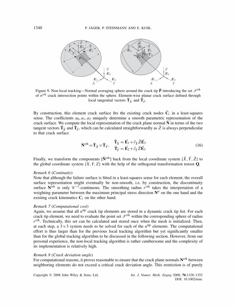
Figure 9. Non-local tracking—Normal averaging sphere around the crack tip P introducing the set Icrk
of ncrk crack intersection points within the sphere. Element-wise planar crack surface defined throughlocal tangential vectors TX and TY .
By construction, this element crack surface fits the existing crack nodes Ci in a least-squaressense. The coefficients a0,a1,a2 uniquely determine a smooth parametric representation of thecrack surface. We compute the local representation of the crack plane normal N in terms of the twotangent vectors TX and TY , which can be calculated straightforwardly as Z is always perpendicularto that crack surface
Ncrk= TX ×TY ,TX = E1+�X Z E3
TY = E2+�Y Z E3(16)
Finally, we transform the components [Ncrk] back from the local coordinate system {X , Y , Z} tothe global coordinate system {X,Y, Z} with the help of the orthogonal transformation tensor Q.
Remark 6 (Continuity)Note that although the failure surface is fitted in a least-squares sense for each element, the overallsurface representation might eventually be non-smooth, i.e. by construction, the discontinuitysurface Ncrk is only C−1-continuous. The smoothing radius rcrk takes the interpretation of aweighting parameter between the maximum principal stress direction N� on the one hand and theexisting crack kinematics Ci on the other hand.
Remark 7 (Computational cost)Again, we assume that all ntip crack tip elements are stored in a dynamic crack tip list. For eachcrack tip element, we need to evaluate the point set Icrk within the corresponding sphere of radiusrcrk. Technically, this set can be calculated and stored once when the mesh is initialized. Then,at each step, a 3×3 system needs to be solved for each of the ntip elements. The computationaleffort is thus larger than for the previous local tracking algorithm but yet significantly smallerthan for the global tracking algorithm to be discussed in the following section. However, from ourpersonal experience, the non-local tracking algorithm is rather cumbersome and the complexity ofits implementation is relatively high.
Remark 8 (Crack deviation angle)For computational reasons, it proves reasonable to ensure that the crack plane normals Ncrk betweenneighboring elements do not exceed a critical crack deviation angle. This restriction is of purely
Copyright q 2008 John Wiley & Sons, Ltd. Int. J. Numer. Meth. Engng 2008; 76:1328–1352DOI: 10.1002/nme
MODELING THREE-DIMENSIONAL CRACK PROPAGATION 1341
algorithmic nature. It has been applied successfully for both local and non-local crack trackingalgorithms in order to avoid spurious zick-zack-type crack surfaces.
Remark 9 (Non-local averaging)As for every non-local averaging scheme, the quality of the averaging procedure strongly relieson the number of crack points ncrk within the averaging set Icrk. A minimum amount of points isessential for the solution of the least-squares problem (15) which in turn crucially influences thequality of the crack tracking algorithm itself. Especially, at the onset of cracking, when the numberof averaging points is rather limited, it seems reasonable to turn off the averaging mechanism andonly switch it on when a sufficiently large number of data points ncrk are available. Then, onecould even think of interpolating the element-wise failure surface through a quadratic rather thana linear approach at only very little extra cost as shown by Gasser and Holzapfel [27, 28].
6. GLOBAL TRACKING
To ensure a unique C0-continuous representation of the discontinuity surfaces in three-dimensionalcrack propagation problems, Oliver and Huespe [34] and Oliver et al. [41] have proposed a robustand yet very elegant strategy that can be incorporated into commercial finite element codes ina remarkably efficient manner. Their initial idea has adopted successfully to simulate discretefracture by Chaves [25], Feist and Hoffstetter [26, 45], Dumstorff and Meschke [43] and Cerveraand Chiumenti [42]. The key feature of Oliver’s global tracking algorithm is to provide isosurfacesI� which in the discrete setting take the interpretation of element-wise planar isopatches. Thesepatches can be described by a function �(X) whose level contours, i.e. the collection of allpatches of �(X)=�I� = const, define the corresponding isosurface I� ={X∈B|�(X)=�I�}.A particular isosurface of constant value, e.g. the surface of level zero �(X)=0, is the kinematicrepresentation of the discrete three-dimensional failure surface. Conceptually speaking, the ultimategoal of the algorithm is to find the scalar field �(X) whose level surfaces are envelopes of thepatches defined by the vectors TX and TY tangential to the propagating discontinuity. Similar to theprevious non-local tracking strategy of Section 5, these tangents to the discontinuity surface, hererepresented in the global coordinate system, obviously obey the orthogonality condition TX ·Ncrk=0and TY ·Ncrk=0 or rather Ncrk=TX ×TY . More importantly, by construction, these patches arealways orthogonal to the gradient of the isosurface �(X), thus TX ·∇�=0 and TY ·∇�=0. Themultiplication of these conditions with TX and TY , respectively, motivates the introduction of aflux vector j=[TX ⊗TX +TY ⊗TY ]·∇�. A reinterpretation of the above considerations in termsof the classical field equations defines an equilibrium equation as the vanishing divergence of thisflux vector j
Div(j)=0 ∀X∈B (17)
and a constitutive equation with the flux being a linear function of the gradient of ∇�
j=D ·∇X� ∀X∈B (18)
The particular format for the anisotropic constitutive tensor D
D=TX ⊗TX +TY ⊗TY (19)
Copyright q 2008 John Wiley & Sons, Ltd. Int. J. Numer. Meth. Engng 2008; 76:1328–1352DOI: 10.1002/nme
1342 P. JAGER, P. STEINMANN AND E. KUHL
ensures that the flux is restricted to the {X , Y }-plane, i.e. it is always a weighted linear combination
of the tangent vectors TX and TY . The problem of finding isosurfaces I� is obviously a classical
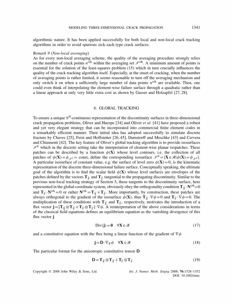
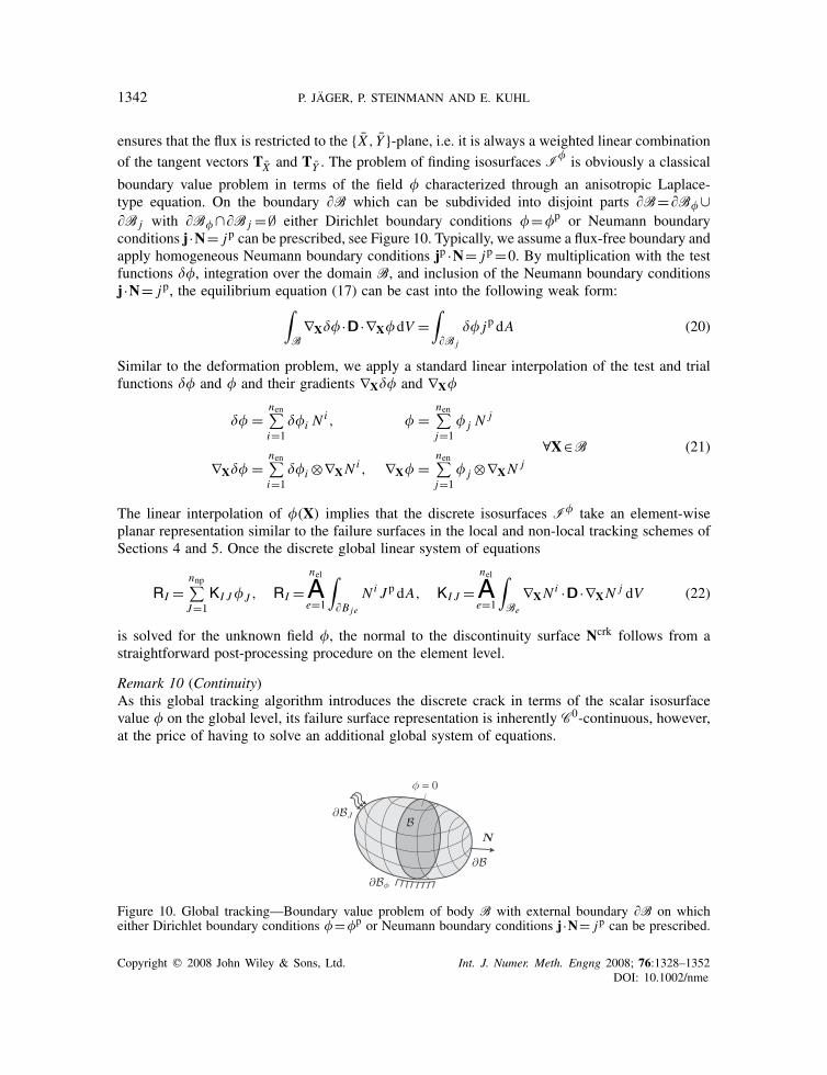
boundary value problem in terms of the field � characterized through an anisotropic Laplace-type equation. On the boundary �B which can be subdivided into disjoint parts �B=�B�∪�B j with �B�∩�B j =∅ either Dirichlet boundary conditions �=�p or Neumann boundaryconditions j ·N= jp can be prescribed, see Figure 10. Typically, we assume a flux-free boundary andapply homogeneous Neumann boundary conditions jp ·N= jp=0. By multiplication with the testfunctions ��, integration over the domain B, and inclusion of the Neumann boundary conditionsj ·N= jp, the equilibrium equation (17) can be cast into the following weak form:∫
B∇X��·D ·∇X�dV =
∫�B j
�� jp dA (20)
Similar to the deformation problem, we apply a standard linear interpolation of the test and trialfunctions �� and � and their gradients ∇X�� and ∇X�
�� =nen∑i=1
��i Ni , � =
nen∑j=1
� j Nj
∇X�� =nen∑i=1
��i ⊗∇XNi , ∇X� =
nen∑j=1
� j ⊗∇XNj
∀X∈B (21)
The linear interpolation of �(X) implies that the discrete isosurfaces I� take an element-wiseplanar representation similar to the failure surfaces in the local and non-local tracking schemes ofSections 4 and 5. Once the discrete global linear system of equations
RI =nnp∑J=1
KI J�J , RI =nel
Ae=1
∫�Bje
N i J p dA, KI J =nel
Ae=1
∫Be
∇XNi ·D ·∇XN
j dV (22)
is solved for the unknown field �, the normal to the discontinuity surface Ncrk follows from astraightforward post-processing procedure on the element level.
Remark 10 (Continuity)As this global tracking algorithm introduces the discrete crack in terms of the scalar isosurfacevalue � on the global level, its failure surface representation is inherently C0-continuous, however,at the price of having to solve an additional global system of equations.
Figure 10. Global tracking—Boundary value problem of body B with external boundary �B on whicheither Dirichlet boundary conditions �=�p or Neumann boundary conditions j ·N= jp can be prescribed.
Copyright q 2008 John Wiley & Sons, Ltd. Int. J. Numer. Meth. Engng 2008; 76:1328–1352DOI: 10.1002/nme

MODELING THREE-DIMENSIONAL CRACK PROPAGATION 1343
Remark 11 (Computational cost)The global tracking algorithm essentially relies on the assembly and solution to an additionalglobal system of equations with one degree of freedom per node. In addition, a neighbor list needsto be initialized ab initio to evaluate average crack tip element values. The total computational costof this algorithm is therefore the highest of all four algorithms discussed in this article. However,the global crack tracking algorithm is also the most flexible and also the most stable of all fouralgorithms. Note that due to its modular nature, its implementation in commercial finite elementcodes is rather straightforward.
Remark 12 (Boundary conditions)As the global crack tracking scheme introduces an additional field of unknowns �, additionalboundary conditions have to be prescribed. To guarantee the invertibility of the system matrix thelevel of the isosurfaces � has to be prescribed at least at two points. The physical interpretation, theunderstanding and the appropriate choice of Dirichlet boundary conditions are the most essentialingredients of the global crack tracking scheme to ensure physically meaningful solutions.
Remark 13 (Invertibility of the anisotropy tensor)To solve the discrete system of Equations (22), the global system matrix K needs to be inverted. Asthe anisotropy tensor D introduced in Equation (19) is rank deficient, we apply slight perturbations� as D=TX ⊗TX +TY ⊗TY +�I to ensure that the overall system is solvable.
Remark 14 (Integration into commercial finite element codes)Although this algorithm has been termed global tracking algorithm it involves only local modi-fications on the element level. It is extremely attractive from a practical point of view as thescalar-valued global degrees of freedom � can be treated as the temperature in Fourier’s heatconduction or as the concentration in Fick’ian diffusion in any standard commercial finite elementprogram. Moreover, the algorithm is in principle able to handle multiple cracking. Owing to itscomputational simplicity, it is extremely robust and stable and highly efficient.
We demonstrate the essential features of the global tracking algorithm in terms of the classicalbenchmark of the L-shaped concrete panel displayed in Figure 11. This geometry was elabo-rated experimentally by Winkler et al. [46]. Previous discrete failure simulations of this classicalbenchmark problem can be found, e.g. in Dumstorff and Meschke [43]. However, their analysis isrestricted to a two-dimensional setting. The L-shaped panel represents a typical example of curved
0 0.1 0.2 0.3 0.4 0.5 0.6 0.7 0.80
1
2
3
4
5
6
7
8
U
F
experiment12969 elements25600 elements32261 elements
Figure 11. L-shaped panel—Geometry and load–displacement curves for global tracking algorithm.
Copyright q 2008 John Wiley & Sons, Ltd. Int. J. Numer. Meth. Engng 2008; 76:1328–1352DOI: 10.1002/nme

1344 P. JAGER, P. STEINMANN AND E. KUHL
cracking that could neither be tackled by the local nor by the non-local tracking algorithm.Obviously, the fixed tracking algorithm cannot be applied either as the failure surface is not knownin advance. Accordingly, the global tracking algorithm is the only strategy that could potentiallybe used to simulate the curved failure surface of the L-shaped panel.
The Lame parameters are �=6161N/mm2 and �=10953N/mm2, the tensile strength is fn =2.7N/mm2, the fracture toughness is Gn =0.065N/mm and the shear stiffness is zero Et =0N/mm. The domain has been discretized with 12 969, 25 600 and 32 261 linear tetrahedralelements, respectively. The load is applied incrementally through displacement control, i.e. theupper left row of nodes is displaced by u=0.02mm in each load steps. The corresponding load–displacement curves and the reference solution to the experimental investigation are displayed inFigure 11 (left). Again, the solution is truly mesh independent and in remarkably good agreementwith the experimental reference curve. Figure 12 shows the stress distribution plotted on thedeformed configuration. The displayed analysis is based on the discretization with 32 261 lineartetrahedral elements and shows the results of load steps 10 and 20, i.e. at an applied deformationof u=0.2 and 0.4mm, respectively. The crack is initiated at the lower corner element. As the loadis increased, the crack propagates smoothly to the right edge of the specimen. Figure 13 shows the
Figure 12. L-shaped panel—Cauchy stress on deformed configuration for load steps 5, 10,15 and 20 for global tracking algorithm.
Figure 13. L-shaped panel—Isosurfaces for load steps 5, 10, 15 and 20 for global tracking algorithm.
Copyright q 2008 John Wiley & Sons, Ltd. Int. J. Numer. Meth. Engng 2008; 76:1328–1352DOI: 10.1002/nme
MODELING THREE-DIMENSIONAL CRACK PROPAGATION 1345
corresponding isosurfaces �(X)=�I� = const at load steps 10 and 20. The discrete failure surfaceis clearly visible. In our simulation, it corresponds to the isosurface of level zero, i.e. �(X)=0,but in general, this value can be chosen arbitrarily.
Remarkably, the crack surface is now no longer planar. This example of the cracked L-shapedpanel has nicely demonstrated the ability of the global crack tracking scheme to simulate thepropagation of curved failure surfaces. It nicely produces smooth C0-continuous arbitrarily shapeddiscontinuity surfaces, however, at the extra cost of solving an additional linear global system ofequations for the values � of the isosurface as scalar-valued nodal unknown. As the coupling of thedeformation field u and the isosurface value field � is rather weak, a staggered solution scheme asthe one presented herein seems to be favorable over a fully coupled simultaneous solution strategy.
7. EXAMPLES
Finally, we will compare the fixed, local, non-local and global tracking algorithm in terms oftwo representative examples. Unfortunately, neither the local nor the non-local crack trackingalgorithm is particularly well suited to simulate curved cracks. Accordingly, we chose to comparethe algorithmic performance in terms of a straight crack problem: the classical three-point bendingtest. Then, we explore a rectangular block under asymmetric tension inducing a curved failuresurface.
7.1. Straight crack—three-point bending test
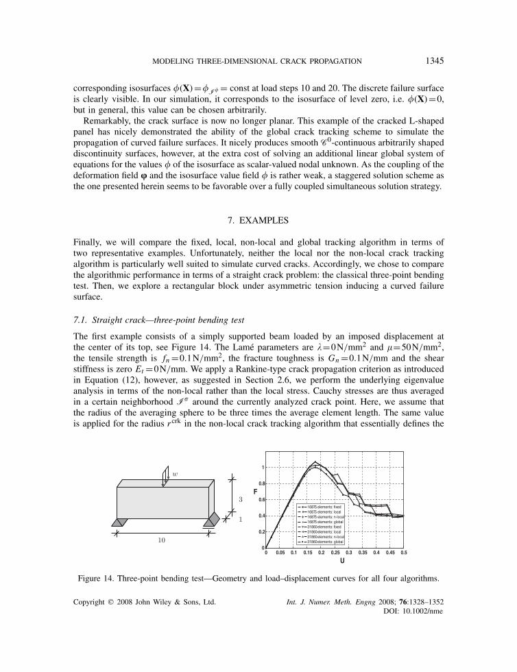
The first example consists of a simply supported beam loaded by an imposed displacement atthe center of its top, see Figure 14. The Lame parameters are �=0N/mm2 and �=50N/mm2,the tensile strength is fn =0.1N/mm2, the fracture toughness is Gn =0.1N/mm and the shearstiffness is zero Et =0N/mm. We apply a Rankine-type crack propagation criterion as introducedin Equation (12), however, as suggested in Section 2.6, we perform the underlying eigenvalueanalysis in terms of the non-local rather than the local stress. Cauchy stresses are thus averagedin a certain neighborhood I� around the currently analyzed crack point. Here, we assume thatthe radius of the averaging sphere to be three times the average element length. The same valueis applied for the radius rcrk in the non-local crack tracking algorithm that essentially defines the
0 0.05 0.1 0.15 0.2 0.25 0.3 0.35 0.4 0.45 0.50
0.2
0.4
0.6
0.8
1
U
F
16875 elements: fixed16875 elements: local16875 elements: n-local16875 elements: global31860elements: fixed31860elements: local31860elements: n-local31860elements: global
Figure 14. Three-point bending test—Geometry and load–displacement curves for all four algorithms.
Copyright q 2008 John Wiley & Sons, Ltd. Int. J. Numer. Meth. Engng 2008; 76:1328–1352DOI: 10.1002/nme
1346 P. JAGER, P. STEINMANN AND E. KUHL
averaging set Icrk for the corresponding crack plane normal. Two different structured meshes with16 875 and 31 860 elements are analyzed. Failure is initialized at the center of the lower face ofthe beam. As expected, due to the symmetric setup the crack path propagates straight upwardsin all four cases. As the discontinuity propagates, we typically observe a change from mode I tomixed mode failure. To overcome the related numerical difficulties we choose to bound the crackdeviation angle to 45◦.
The corresponding load–displacement curves for the coarse 16875 element mesh and the finer31860 element mesh are displayed in Figure 14 for both the fixed, the local, the non-local andthe global crack tracking algorithm. Obviously, the response is independent of the applied cracktracking strategy. The proposed failure criterion depends on the maximum tensile strength of allelements within an averaging sphere that has a radius of three times the average element length.Accordingly, the larger elements of the coarse mesh fail slightly later and the peak load is a littleoverestimated for the coarse discretization, see Figure 14. Apart from this effect, the good agreementof the eight curves confirms the objectivity of both methods with respect to the discretization.
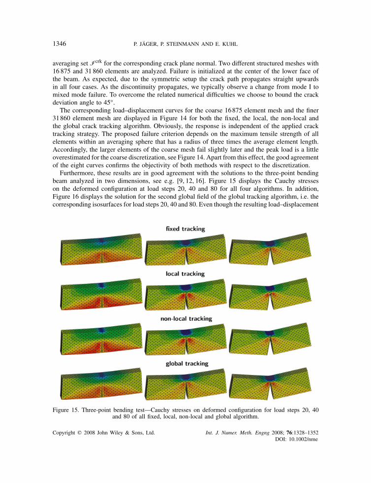
Furthermore, these results are in good agreement with the solutions to the three-point bendingbeam analyzed in two dimensions, see e.g. [9, 12, 16]. Figure 15 displays the Cauchy stresseson the deformed configuration at load steps 20, 40 and 80 for all four algorithms. In addition,Figure 16 displays the solution for the second global field of the global tracking algorithm, i.e. thecorresponding isosurfaces for load steps 20, 40 and 80. Even though the resulting load–displacement
Figure 15. Three-point bending test—Cauchy stresses on deformed configuration for load steps 20, 40and 80 of all fixed, local, non-local and global algorithm.
Copyright q 2008 John Wiley & Sons, Ltd. Int. J. Numer. Meth. Engng 2008; 76:1328–1352DOI: 10.1002/nme
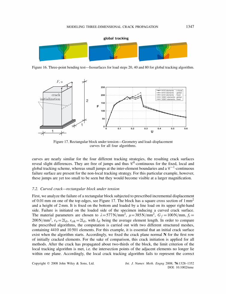
MODELING THREE-DIMENSIONAL CRACK PROPAGATION 1347
Figure 16. Three-point bending test—Isosurfaces for load steps 20, 40 and 80 for global tracking algorithm.
0 0.1 0.2 0.3 0.4 0.5 0.60
50
100
150
200
250
U
F
4410 elements - n-local4410 elements - global4410 elements - fixed10501 elements - global10501 elements - fixed
1
1
2
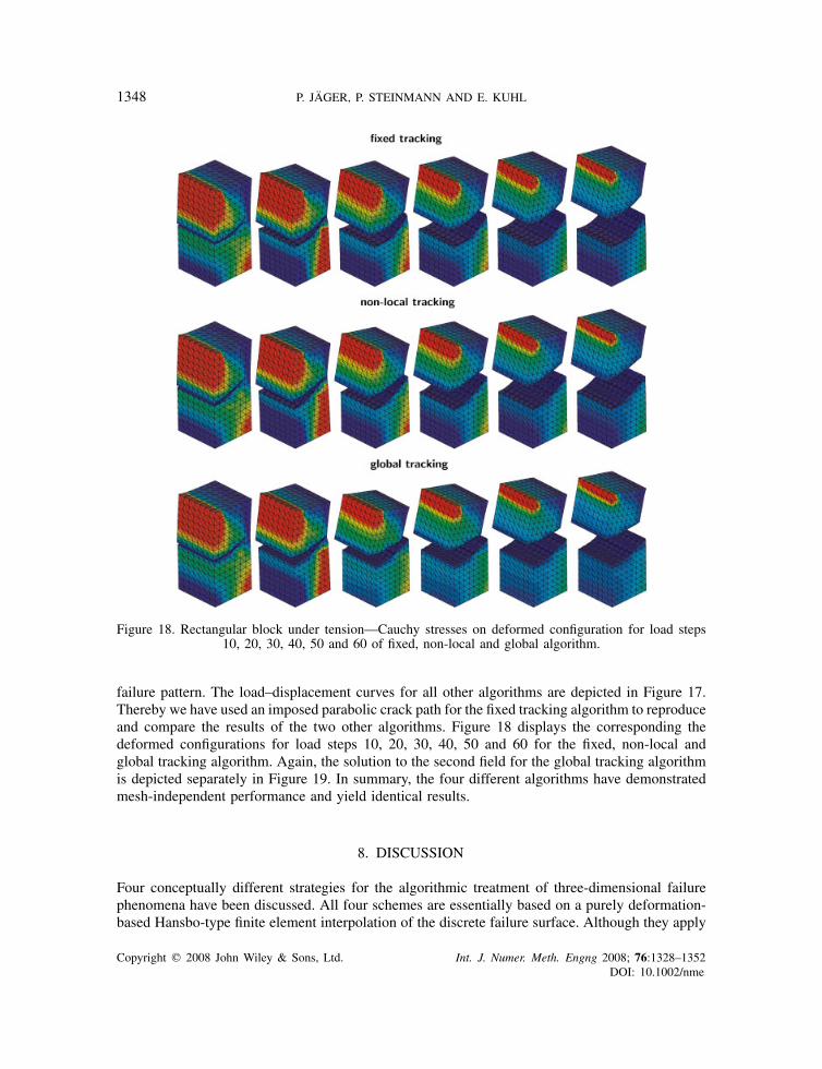
Figure 17. Rectangular block under tension—Geometry and load–displacementcurves for all four algorithms.
curves are nearly similar for the four different tracking strategies, the resulting crack surfacesreveal slight differences. They are free of jumps and thus C0-continuous for the fixed, local andglobal tracking scheme, whereas small jumps at the inter-element boundaries and a C−1-continuousfailure surface are present for the non-local tracking strategy. For this particular example, however,these jumps are yet too small to be seen but they would become visible at a larger magnification.
7.2. Curved crack—rectangular block under tension
First, we analyze the failure of a rectangular block subjected to prescribed incremental displacementof 0.01mm on one of the top edges, see Figure 17. The block has a square cross section of 1mm2
and a height of 2mm. It is fixed on the bottom and loaded by a line load on its upper right-handside. Failure is initiated on the loaded side of the specimen inducing a curved crack surface.The material parameters are chosen to �=577N/mm2, �=385N/mm2, G f =100N/mm, ft =200N/mm2, r� =2lel, rcrk=2lel, with lel being the average element length. In order to comparethe prescribed algorithms, the computation is carried out with two different structured meshes,containing 4410 and 10 501 elements. For this example, it is essential that an initial crack surfaceexist when the algorithm starts. Accordingly, we fixed the crack plane normal N for the first rowof initially cracked elements. For the sake of comparison, this crack initiation is applied for allmethods. After the crack has propagated about two-thirds of the block, the limit criterion of thelocal tracking algorithm is met, i.e. the intersection points of the adjacent elements no longer liewithin one plane. Accordingly, the local crack tracking algorithm fails to represent the correct
Copyright q 2008 John Wiley & Sons, Ltd. Int. J. Numer. Meth. Engng 2008; 76:1328–1352DOI: 10.1002/nme
1348 P. JAGER, P. STEINMANN AND E. KUHL
Figure 18. Rectangular block under tension—Cauchy stresses on deformed configuration for load steps10, 20, 30, 40, 50 and 60 of fixed, non-local and global algorithm.
failure pattern. The load–displacement curves for all other algorithms are depicted in Figure 17.Thereby we have used an imposed parabolic crack path for the fixed tracking algorithm to reproduceand compare the results of the two other algorithms. Figure 18 displays the corresponding thedeformed configurations for load steps 10, 20, 30, 40, 50 and 60 for the fixed, non-local andglobal tracking algorithm. Again, the solution to the second field for the global tracking algorithmis depicted separately in Figure 19. In summary, the four different algorithms have demonstratedmesh-independent performance and yield identical results.
8. DISCUSSION
Four conceptually different strategies for the algorithmic treatment of three-dimensional failurephenomena have been discussed. All four schemes are essentially based on a purely deformation-based Hansbo-type finite element interpolation of the discrete failure surface. Although they apply
Copyright q 2008 John Wiley & Sons, Ltd. Int. J. Numer. Meth. Engng 2008; 76:1328–1352DOI: 10.1002/nme
MODELING THREE-DIMENSIONAL CRACK PROPAGATION 1349
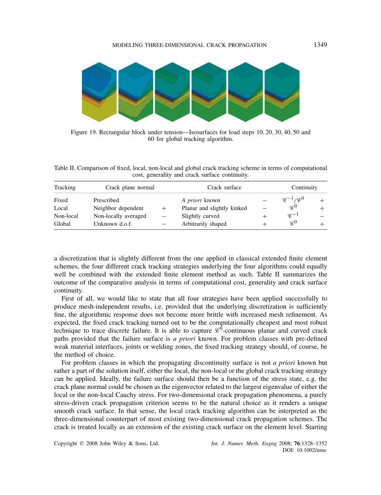
Figure 19. Rectangular block under tension—Isosurfaces for load steps 10,20,30,40,50 and60 for global tracking algorithm.
Table II. Comparison of fixed, local, non-local and global crack tracking scheme in terms of computationalcost, generality and crack surface continuity.
Tracking Crack plane normal Crack surface Continuity
Fixed Prescribed A priori known − C−1/C0 +Local Neighbor dependent + Planar and slightly kinked − C0 +Non-local Non-locally averaged − Slightly curved + C−1 −Global Unknown d.o.f. − Arbitrarily shaped + C0 +
a discretization that is slightly different from the one applied in classical extended finite elementschemes, the four different crack tracking strategies underlying the four algorithms could equallywell be combined with the extended finite element method as such. Table II summarizes theoutcome of the comparative analysis in terms of computational cost, generality and crack surfacecontinuity.
First of all, we would like to state that all four strategies have been applied successfully toproduce mesh-independent results, i.e. provided that the underlying discretization is sufficientlyfine, the algorithmic response does not become more brittle with increased mesh refinement. Asexpected, the fixed crack tracking turned out to be the computationally cheapest and most robusttechnique to trace discrete failure. It is able to capture C0-continuous planar and curved crackpaths provided that the failure surface is a priori known. For problem classes with pre-definedweak material interfaces, joints or welding zones, the fixed tracking strategy should, of course, bethe method of choice.
For problem classes in which the propagating discontinuity surface is not a priori known butrather a part of the solution itself, either the local, the non-local or the global crack tracking strategycan be applied. Ideally, the failure surface should then be a function of the stress state, e.g. thecrack plane normal could be chosen as the eigenvector related to the largest eigenvalue of either thelocal or the non-local Cauchy stress. For two-dimensional crack propagation phenomena, a purelystress-driven crack propagation criterion seems to be the natural choice as it renders a uniquesmooth crack surface. In that sense, the local crack tracking algorithm can be interpreted as thethree-dimensional counterpart of most existing two-dimensional crack propagation schemes. Thecrack is treated locally as an extension of the existing crack surface on the element level. Starting
Copyright q 2008 John Wiley & Sons, Ltd. Int. J. Numer. Meth. Engng 2008; 76:1328–1352DOI: 10.1002/nme
1350 P. JAGER, P. STEINMANN AND E. KUHL
from the crack intersection points of the neighboring element, the crack propagates smoothly basedon the principal stress direction with slight adjustments based on the neighboring crack points. It isquite obvious that this local crack tracking strategy always produces C0-continuous failure surfacesat extremely low computational cost. Unfortunately, however, these surfaces might eventuallybe over-constrained in the case of too many pre-existing neighbor crack points. Accordingly,the failure surface typically hardly deviates from a planar or slightly kinked crack path and thestructural stiffness would be severely overestimated. In summary, if the failure surface is expectedto be rather planar or only slightly kinked, we would advise to use the stable, cheap and robustlocal crack tracking scheme. In all other cases, a non-local or global tracking scheme should beapplied.
To predict failure surfaces of arbitrary shape, the discrete failure surface introduced on theelement level essentially needs to incorporate information of the surrounding elements. Withina finite element setting, there are two fundamentally different ways to carry information of acertain neighborhood to the element or rather the integration point level. The first method smoothesthe failure surface in a least-squares sense based on the non-locally averaged information withina certain neighborhood. This method is local in the sense that it does not introduce additionalglobal degrees of freedom. Accordingly, however, the generated failure surfaces might showslight jumps at the inter-element boundaries. The non-local crack tracking scheme might becomputationally cheaper than the global one as it does not rely on the solution of an additionalsystem of equations. Nevertheless, its underlying algorithmic changes are quite cumbersome andintegration into commercial finite element codes would require sophisticated modifications on theintegration point level, on the element level and on the system level.
An alternative strategy that is somewhat more tailored to the notion of finite elements isthe global crack tracking scheme. At the expense of introducing an additional scalar-valuedfield of unknowns and having to invert the related system matrix, the global tracking schemeis the only one that really combines advantages of all the previous schemes. It is robust andstable, it is able to reliably capture smooth, curved, arbitrarily shaped C0-continuous failuresurfaces and it is straightforwardly integratable into commercial finite element codes. The globalcrack tracking strategy is the most general of all analyzed schemes and thus applicable inall cases where the failure surface is not a priori known and not necessarily expected to beplanar.
A comprehensive series of numerical benchmark tests for all four schemes has been performedbut only illustrative examples have been presented in this article. The incorporation of the suggestedcrack tracking strategies into commercial finite element codes that will ultimately allow formore realistic large-scale computations is part of this research. Based on our preliminary studies,however, we believe that especially the global crack tracking strategy has great potential to success-fully predict discrete failure phenomena in various kinds of industrially relevant applications andwould therefore strongly advocate to incorporate it in commercial finite element codes in the nearfuture.
ACKNOWLEDGEMENTS
This work is part of the research project carried out within the DFG Graduate School 814 ‘Engineeringmaterials on different scales’. We would kindly like to acknowledge its support through the GermanNational Science Foundation. Moreover, we would like to thank Thomas Christian Gasser for his intensivedetailed discussions and helpful advise.
Copyright q 2008 John Wiley & Sons, Ltd. Int. J. Numer. Meth. Engng 2008; 76:1328–1352DOI: 10.1002/nme
MODELING THREE-DIMENSIONAL CRACK PROPAGATION 1351
REFERENCES
1. Armero F, Garikipati K. An analysis of strong discontinuities in multiplicative finite strain plasticity and theirrelation with the numerical simulation of strain localization in solids. International Journal of Solids and Structures1996; 33(20–22):2863–2885.
2. Dvorkin EN, Cuitino AM, Gioia G. Finite-elements with displacement interpolated embedded localization linesinsensitive to meshsize and distortions. International Journal for Numerical Methods in Engineering 1990;30(3):541–564.
3. Oliver J. Modelling strong discontinuities in solid mechanics via strain softening constitutive equations.1. Fundamentals. International Journal for Numerical Methods in Engineering 1996; 39(21):3575–3600.
4. Oliver J. Modelling strong discontinuities in solid mechanics via strain softening constitutive equations.2. Numerical simulation. International Journal for Numerical Methods in Engineering 1996; 39(21):3601–3623.
5. Sluys LJ, Berend AH. Discontinuous failure analysis for mode-I and mode-II localization problems. InternationalJournal of Solids and Structures 1998; 35(31–32):4257–4274.
6. Simo JC, Armero F, Taylor RL. Improved versions of assumed enhanced strain tri-linear elements for 3D-finitedeformation problems. Computer Methods in Applied Mechanics and Engineering 1993; 110(3–4):359–386.
7. Belytschko T, Moes M, Usui S, Parimi C. Arbitrary discontinuities in finite elements. International Journal forNumerical Methods in Engineering 2001; 50(4):993–1013.
8. Dolbow J, Moes N, Belytschko T. Discontinuous enrichment in finite elements with a partition of unity method.Finite Elements in Analysis and Design 2000; 36(3–4):235–260.
9. de Borst R. Numerical aspects of cohesive-zone models. Engineering Fracture Mechanics 2003; 70(14):1743–1757.
10. de Borst R, Guitierrez MA, Wells GN, Remmers JC, Askes H. Cohesive-zone models, higher-order continuumtheories and reliability methods for computational failure analysis. International Journal for Numerical Methodsin Engineering 2004; 60(1):289–315.
11. Remmers JJC, de Borst R, Needleman A. A cohesive segments method for the simulation of crack growth.Computational Mechanics 2003; 31(1–2):69–77.
12. Wells GN, Sluys LJ. A new method for the modelling of cohesive cracks using finite elements. InternationalJournal for Numerical Methods in Engineering 2001; 50(12):2667–2682.
13. Wells GN, Sluys LJ, de Borst R. Simulating the propagation of displacement discontinuities in a regularizedstrain-softening medium. International Journal for Numerical Methods in Engineering 2002; 53(5):1235–1256.
14. Hansbo A, Hansbo P. A finite element method for the simulation of strong and weak discontinuities in solidmechanics. Computer Methods in Applied Mechanics and Engineering 2004; 193(33–35):3532–3540.
15. Hansbo A, Hansbo P, Larson MG. A finite element method on composite grids based on Nitsche’s method.ESAIM: Mathematical Modelling and Numerical Analysis 2003; 37(3):495–514.
16. Kuhl E, Jager P, Mergheim J, Steinmann P. On the application of Hansbo’s method for interface problems. InProceedings of the IUTAM Symposium on Discretization Methods for Evolving Discontinuities, Lyon, France,Combescure A, de Borst R, Belytschko T (eds). Springer: Berlin, 2006.
17. Mergheim J, Kuhl E, Steinmann P. A hybrid discontinuous Galerkin/interface method for the computationalmodelling of failure. Communications in Numerical Methods in Engineering 2004; 20(7):511–519.
18. Mergheim J, Kuhl E, Steinmann P. A finite element method for the computational modelling of cohesive cracks.International Journal for Numerical Methods in Engineering 2005; 63(2):276–289.
19. Mergheim J, Kuhl E, Steinmann P. Towards the algorithmic treatment of 3D strong discontinuities. Communicationsin Numerical Methods in Engineering 2007; 23(2):97–108.
20. Areias PMA, Belytschko T. A comment on the article ‘A finite element method for the simulation of strongand weak discontinuities in solid mechanics’ by A. Hansbo and P. Hansbo [Computer Methods in AppliedMechanics and Engineering 2004; 193:3523–3540]. Computer Methods in Applied Mechanics and Engineering2006; 195(9–12):1275–1276.
21. Areias PMA, Song JH, Belytschko T. Analysis of fracture in thin shells by overlapping paired elements. ComputerMethods in Applied Mechanics and Engineering 2006; 195(41–43):5343–5360.
22. Jager P, Steinmann P, Kuhl E. On local tracking algorithms for the simulation of three-dimensional discontinuities.Computational Mechanics 2007; DOI: 10.1007/s00466-008-0249-3.
23. Meschke G, Dumstorff P. Energy-based modeling of cohesive and cohesionless cracks via X-FEM. ComputerMethods in Applied Mechanics and Engineering 2007; 196(21–24):2338–2357.
24. Areias PMA, Belytschko T. Analysis of three-dimensional crack initiation and propagation using the extendedfinite element method. International Journal for Numerical Methods in Engineering 2005; 63(5):760–788.
Copyright q 2008 John Wiley & Sons, Ltd. Int. J. Numer. Meth. Engng 2008; 76:1328–1352DOI: 10.1002/nme

1352 P. JAGER, P. STEINMANN AND E. KUHL
25. Chaves EWV. Tracking 3D crack path. Proceedings of the International Conference on Mathematical andStatistical Modeling in Honor of Enrique Castillo. ICMSM Ciudad Real: Spain, 2006.
26. Feist C, Hofstetter G. Three-dimensional fracture simulations based on the SDA. International Journal forNumerical and Analytical Methods in Geomechanics 2007; 31(2):189–212.
27. Gasser TC, Holzapfel GA. Modeling 3D crack propagation in unreinforced concrete using PUFEM. ComputerMethods in Applied Mechanics and Engineering 2005; 194(25–26):2859–2896.
28. Gasser TC, Holzapfel GA. 3D Crack propagation in unreinforced concrete. A two-step algorithm for tracking3D crack paths. Computer Methods in Applied Mechanics and Engineering 2006; 195(37–40):5198–5219.
29. Gasser TC. Validation of 3D crack propagation in plain concrete. Part II: computational modeling and predictionsof the PCT3D test. Computers and Concrete 2007; 4(1):67–82.
30. Gravouil A, Moes N, Belytschko T. Non-planar 3D crack growth by the extended finite element and level sets—Part II: level set update. International Journal for Numerical Methods in Engineering 2002; 53(11):2569–2586.
31. Mosler J, Meschke G. 3D modelling of strong discontinuities in elastoplastic solids: fixed and rotating localizationformulations. International Journal for Numerical Methods in Engineering 2003; 57(11):1553–1576.
32. Mosler J. Modeling strong discontinuities at finite strains—a novel numerical implementation. Computer Methodsin Applied Mechanics and Engineering 2006; 195(33–36):4396–4419.
33. Moes N, Gravouil A, Belytschko T. Non-planar 3D crack growth by the extended finite element and level sets—Part I: mechanical model. International Journal for Numerical Methods in Engineering 2002; 53(11):2549–2568.
34. Oliver J, Huespe AE. On strategies for tracking strong discontinuities in computational failure mechanics. InProceedings of the Fifth World Congress on Computational Mechanics (WCCM V), Vienna, Austria, Mang HA,Rammersdorfer FG, Erberhardsteiner J (eds). 2002.
35. Pandolfi A, Ortiz M. An efficient adaptive procedure for three-dimensional fragmentation simulations. EngineeringComputations 2002; 18(2):148–159.
36. Rabczuk T, Belytschko T. A three dimensional large deformation meshfree method for arbitrary evolving cracks.Computer Methods in Applied Mechanics and Engineering 2007; 196:2777–2799.
37. Ruiz G, Ortiz M, Pandolfi A. Three-dimensional finite-element simulation of the dynamic Brazilian tests onconcrete cylinders. International Journal for Numerical Methods in Engineering 2000; 48(7):963–994.
38. Sancho JM, Planas J, Fathy AM, Galvez JC, Cendon DA. Three-dimensional simulation of concrete fractureusing embedded crack elements without enforcing crack path continuity. International Journal for Numericaland Analytical Methods in Geomechanics 2007; 31(2):173–187.
39. Sukumar N, Moes N, Moran B, Belytschko T. Extended finite element method for three-dimensional crackmodelling. International Journal for Numerical Methods in Engineering 2000; 48(11):1549–1570.
40. Feist C, Hofstetter G. Crack propagation in plain concrete. Part I: experimental investigation—the PCT3D test.Computers and Concrete 2007; 4(1):49–66.
41. Oliver J, Huespe AE, Samaniego E, Chaves EVW. Continuum approach to the numerical simulation ofmaterial failure in concrete. International Journal for Numerical and Analytical Methods in Geomechanics 2004;28(7–8):609–632.
42. Cervera M, Chiumenti M. Mesh objective tensile cracking via a local continuum damage model and a cracktracking technique. Computer Methods in Applied Mechanics and Engineering 2006; 196(1–3):304–320.
43. Dumstorff P, Meschke G. Crack propagation criteria in the framework of X-FEM-based structural analyses.International Journal for Numerical and Analytical Methods in Geomechanics 2007; 31(2):239–259.
44. Jirasek M, Rolshoven S, Grassl P. Size effects on fracture energy induced by non-locality. International Journalfor Numerical and Analytical Methods in Geomechanics 2004; 28(7–8):653–670.
45. Feist C, Hofstetter G. An embedded strong discontinuity model for cracking of plain concrete. Computer Methodsin Applied Mechanics and Engineering 2006; 195(52):7115–7138.
46. Winkler BJ, Hofstetter G, Niederwanger G. Experimental verification of a constitutive model for concrete cracking.Proceedings of the Institution of Mechanical Engineers, Part L: Journal of Materials—Design and Applications2001; 215(L2):75–86.
Copyright q 2008 John Wiley & Sons, Ltd. Int. J. Numer. Meth. Engng 2008; 76:1328–1352DOI: 10.1002/nme