Embed Size (px)
Citation preview
International Journal of Sciences: Basic and Applied Research
(IJSBAR)
ISSN 2307-4531 (Print & Online)
http://gssrr.org/index.php?journal=JournalOfBasicAndApplied
--------------------------------------------------------------------------------------------------------------------
Predicting the Volatility of Stock Markets and Measuring its Interaction with Macroeconomic Variables: Indian
Evidence, Case Study of NIFTY and SENSEX
Amit Kumar Jhaa*, Nitesh Kumar Singhb aM.Phil, Delhi School of Economics, University of Delhi, Delhi-110007
bResearch Assistant, CUTS-International, Jaipur, Rajasthan-302016
aE-mail: [email protected]
bE-mail: [email protected]
Abstract
This paper investigates the effects of economic factors on India’s stock markets. It utilized Johansen cointegration
test and Innovation Accounting techniques to study the short-run dynamics as well as long-run relationship between
stock prices and four macroeconomic variables from the Indian economy. It also attempts to forecast the volatility of
stock markets with the help from Autoregressive Conditional Heteroskedastic models (ARCH). We found co-
movements between stock market index and macroeconomic variables in a long-run equilibrium path. The variations
in the stock prices are mainly attributed to its own variations and to smaller extent by other macroeconomic
variables. EGARCH method emerged as the best forecasting tool available, among others. However, it is advisable
not to forecast beyond one period in cases of such volatile series, because of the randomness involved as visible
from the forecast errors obtained from different methods.
Keywords: Volatility; Stock prices; Macroeconomic Variables; Forecasting
1. Introduction
The relationship between macro-economic factors and stock market developments has been the subject of interest
among researchers over the last two decades.
------------------------------------------------------------------ *Corresponding author. E-mail address:[email protected]
371
brought to you by COREView metadata, citation and similar papers at core.ac.uk
provided by GSSRR.ORG: International Journals: Publishing Research Papers in all Fields

International Journal of Sciences: Basic and Applied Research (IJSBAR) (2014) Volume 13, No 1, pp 371-393 It has often been argued that some fundamental macroeconomic factors such as exchange rate, interest rate, and
inflation are the key determinants of stock prices. Chen, Rolland and Ross [1] showed that economic state variables
do tend to affect future dividends as well as discount rate and thus stock prices. Fama [2] also showed a strong
positive correlation between common stock returns and real variables such as capital expenditure, industrial
production, GNP, money supply and interest rate.
Until recently, the most widely used framework in this regard was the arbitrage pricing theory(APT) model which,
in finance is a general theory of asset pricing which has become influential in the pricing of stocks. APT holds that
the expected return of a financial asset can be modeled as a linear function of various macro-economic factors or
theoretical market indices, where sensitivity to changes in each factor is represented by a factor-specific beta
coefficient. The model-derived rate of return will then be used to price the asset correctly - the asset price should
equal the expected end of period price discounted at the rate implied by model. If the price diverges, arbitrage
should bring it back into line. However, with the development of cointegration analysis, has allowed for another
approach to examine the relationship between economic variables and stock markets. An advantage of co-integration
analysis has been the realization of the dynamic comovements among the variables and adjustment process towards
the long term equilibrium could be examined. Mukherjee and Naka [3] employed Johansen co-integration test in the
vector error correction model (VECM) and found that Japanese stock market was cointegrated with six
macroeconomic variables. Mayasmai and Koh[4] used the same analysis for Singapore stock market and found it to
be cointegrated with five macroeconomic variables.
This paper extends the same analysis on the Indian stock markets which is represented by Bombay stock exchange
(BSE) where the index chosen is SENSEX. The BSE Index, SENSEX, is India's first stock market index that enjoys
an iconic stature, and is tracked worldwide. It is an index of 30 stocks representing 12 major sectors. The SENSEX
is constructed on a 'free-float' methodology, and is sensitive to market sentiments and market realities. The objective
is to investigate the dynamic relationship between stock prices and four macroeconomic variables. The important
contribution of this paper towards the exiting literature would be the inclusion of more pronounced set of variables
which can truly reflect the broader picture of the factors affecting the stock markets.
Second objective of this paper is concerned with predicting the volatility of stock markets. The volatility quantifies
the uncertainty about future asset price fluctuations. To model and forecast stock market volatility has been the
subject of much recent empirical and theoretical investigation by academics and practitioners alike. First, volatility
has received a great deal of concern from policy makers and financial market participants because it can be used as a
measurement of risk. Second, greater volatility in the stock, bond and foreign exchange markets has raised important
public policy issues about the stability of financial markets and the impact of volatility on the economy. Therefore
another goal of this paper is to investigate the extent to which, it is possible to predict the volatility of NIFTY’s
weekly index(The NSE's key index is the S&P CNX NIFTY, known as the Nifty, an index of fifty major stocks
weighted by market capitalization) which has been a major indicator for National Stock Exchange. The rest of the
paper is organized as follow: Second section covers the relationship between macroeconomic variables and stock
markets. Third will review the literatures, while fourth describes data sources and definitions and fifth section will
capture the methodology. Finally, sixth section will present empirical results and conclusions.
372

International Journal of Sciences: Basic and Applied Research (IJSBAR) (2014) Volume 13, No 1, pp 371-393 2. Relationship between Macroeconomic variables and stock price movements:
This study has looked upon the following variables:
• Interest rate (INT)
• Exchange rate (EXRATE)
• Money supply (M3)
• Net inflows of Foreign Institutional Investors (FIIs)
The intuition behind the relationship between interest rates and stock prices is straightforward. An increase in the
rate of interest raises the opportunity cost of holding cash and is likely to lead to a substitution effect between stocks
and other interest bearing securities. Additionally, changes in interest rates are expected to affect the discount rate in
the same direction via their effect on the nominal risk-free rate
The exchange rate being measured in terms of dollars is expected to have a positive relationship with stock prices.
Solnik [5] indicated that both exchange rate levels and changes affect the performance of a stock market. For an
export-dominated country, currency depreciation will have a favorable impact on the domestic stock market, as the
product exported from the country will become cheaper in the foreign countries. As a result, if the demand for goods
exported is elastic, the volume of exports would increase, which in turn would cause higher cash flows and thus a
surge in the stock prices of domestic companies. The opposite should hold in case of appreciation. It is also
hypothesized that trade balance is positively related with stock prices, as it is a possible indicator of country’s
competitiveness and its performance on economic front.
The effect of money supply on stock prices is also a matter of empirical proof. Since the rate of inflation is
positively related to money growth rate [2], an increase in the money supply may lead to an increase in the discount
rate and lower stock prices. However, this negative effect may be countered by the economic stimulus provided by
money growth, which would likely increase cash flows and stock prices [3].
Lastly FIIs, over the years, have been allowed to operate in Indian stock markets. It now includes institutions such as
pension funds, mutual funds, investment trusts, asset management companies etc. Therefore it’s appropriate to
hypothesize a positive relation between FIIs inflows and stock markets.
3. Literature reviews
Hagen H.W. Bluhm, JunYu[6] compared two basic approaches to forecast volatility in the German stock market.
The first approach used various univariate time series techniques while the second approach made use of volatility
implied in option prices. It was showed that the model rankings were sensitive to the error measurements as well as
the forecast horizons. The result indicated that it was difficult to state which method was the clear winner. Mats
Palmquist, Björn Viman [7] investigated the extent to which it is possible to predict the volatility for the OMX-index
and further to compare, evaluate and rank the methods used, to see which one predicts most accurately. In this paper,
simpler methods like historical average and random walk and more complex methods like EWMA (Exponential
373

International Journal of Sciences: Basic and Applied Research (IJSBAR) (2014) Volume 13, No 1, pp 371-393 weighted moving average) and GARCH (1, 1) were used. Overall, the forecast results with EWMA estimators were
very close to the forecast result with the more complicated GARCH (1, 1) model. The random walk performed
second worst and the historical average the worst. Chris Brooks [8] explored a number of statistical models for
predicting the daily stock return volatility of an aggregate of all stocks traded on the NYSE. An application of linear
and non-linear Granger causality tests highlighted evidence of bidirectional causality, although the relationship was
stronger from volatility to volume than the other way around.
Madhusudan Karmakar [9] estimated conditional volatility models in an effort to capture the salient features of stock
market volatility in India and evaluate the models in terms of out-of sample forecast accuracy. It also investigated
whether there was any leverage effect in Indian companies. Nikolay Gospodinov, Athanasia Gavala, Deming Jiang
[10] investigated the time series properties of S&P 100 volatility and the forecasting performance of different
volatility models. It considered several nonparametric and parametric volatility measures, such as implied, realized
and model-based volatility, and showed that these volatility processes exhibit an extremely slow mean-reverting
behavior and possible long memory. Amita Batra [11] analyzed time variation in volatility in the Indian stock
market during 1979-2003. It examined if there had been an increase in volatility persistence in the Indian stock
market on account of the process of financial liberalization in India. The analysis revealed that the period around the
BOP crisis and the initiation of economic reforms in India was the most volatile period in the stock market.
Structural shifts in volatility were more likely to be a consequence of major policy changes and any further
incremental policy changes may had only a benign influence on stock return volatility.
H.R. Badrinath and Prakash G. Apte [12] examined the stock market, the foreign exchange market and the call
money market in India for evidence of volatility spillovers using multivariate EGARCH models which facilitated the
study of asymmetric responses. The results indicated the existence of asymmetric volatility spillovers across these
markets. The results also indicated that either the information assimilation across markets was slow or that the
spillovers were on account of contagion. Gautam Goswami and Sung-Chang Jung [13] investigated the effects of
economic factors on Korean stock market. It used Vector Error Correction Model (VECM), and looked at the short-
run dynamics as well as long-run relationship between stock price and nine macroeconomic variables from Korean
economy. It was found that the Korean stock market was co-integrated with nine macroeconomic variables. The
Korean stock prices were positively related to industrial production, inflation and short-term interest rate, and
negatively related to long-term interest rates and oil prices. Anokye M. Adam, George Tweneboah[14] examined
the role of macroeconomic variables on stock prices movement in Ghana. It used the Databank stock index to
represent Ghana stock market and (a) inward foreign direct investments, (b) the treasury bill rate (as a measure of
interest rates), (c) the consumer price index (as a measure of inflation), and (d) the exchange rate as macroeconomic
variables. It established cointegration between macroeconomic variables identified and Stock prices in Ghana, which
indicated long run relationship. Results of Impulse Response Function (IRF) and Forecast Error Variance
Decomposition (FEVD) indicated that interest rate and Foreign Direct Investment (FDI) were the key determinants
of the share price movements in Ghana.
Ramin Cooper Maysami, Tiong Sim Koh [4] examined the long-term equilibrium relationships between the
Singapore stock index and selected macroeconomic variables, as well as among stock indices of Singapore, Japan,
374

International Journal of Sciences: Basic and Applied Research (IJSBAR) (2014) Volume 13, No 1, pp 371-393 and the United States. With help from appropriate vector error-correction models, it detected that changes in two
measures of real economic activities, industrial production and trade, were not integrated of the same order as
changes in Singapore’s stock market levels. However, changes in Singapore’s stock market levels did form a co-
integrating relationship with changes in price levels, money supply, short- and long-term interest rates, and
exchange rates. While changes in interest and exchange rates contributed significantly to the co-integrating
relationship, those in price levels and money supply did not. Christopher Gan, Minsoo Lee, Hua Hwa Au Yong, Jun
Zhang [15] employed co-integration tests and examined the relationships between the New Zealand Stock Index and
a set of seven macroeconomic variables from January 1990 to January 2003.Specifically, it employed the Johansen
Maximum Likelihood and Granger-causality tests to determine whether the New Zealand Stock Index was a leading
indicator for macroeconomic variables. They found that NZSE40 was consistently determined by the interest rate,
money supply and real GDP and no evidence was found that the New Zealand Stock Index was a leading indicator
for changes in macroeconomic variables. Nai-Fu Chen, Richard Roll and Stephen A. Ross [1] examined whether
innovations in macroeconomic variables are risks that are rewarded in stock market. The variables included were
spread between long and short term interest rates, index of industrial production, spread between high and low grade
bonds and expected and unexpected inflations. It was found that these sources of risk were significantly priced.
Further, neither the market portfolio nor the aggregate consumption was priced separately. Andreas Humpe and
Peter Macmillan [16] analysed within the framework of a standard discounted value model, whether a number of
macroeconomic variables influenced stock prices in the US and Japan. A cointegration analysis was applied in order
to model the long term relationship between industrial production, the consumer price index, money supply, long
term interest rates and stock prices in the US and Japan. For the US, it was found that the data was consistent with a
single cointegrating vector, where stock prices were positively related to industrial production and negatively related
to both the consumer price index and a long term interest rate. However, for the Japanese data, two cointegrating
vectors were found. For one vector, the stock prices were influenced positively by industrial production and
negatively by the money supply. For the second cointegrating vector, industrial production was found to be
negatively influenced by the consumer price index and a long term interest rate.
Nil Günsel and Sadõk Çukur [17] investigated the performance of the Arbitrage Pricing Theory (APT) in London
Stock Exchange for the period of 1980-1993 as monthly. The study developed seven pre-specified macroeconomic
variables. The term structure of interest rate, the risk premium, the exchange rate, the money supply and
unanticipated inflation were similar to those derived in Chen, Roll and Ross [1]. Ramin Cooper Maysami, Lee
Chuin Howe and Mohamad Atkin Hamzah[18] looked at the long-term equilibrium relationships between selected
macroeconomic variables and the Singapore stock market index (STI), as well as with various Singapore Exchange
Sector indices—the finance index, the property index, and the hotel index was examined. The study concluded that
the Singapore’s stock market and the property index form cointegrating relationship with changes in the short and
long-term interest rates, industrial production, price levels, exchange rate and money supply.
4. Data
For the first objective, a total of four macroeconomic variables and BSE SENSEX data are used. All variables are in
natural logarithm and are monthly frequencies from January 2000 to December 2008. However, for the second
375

International Journal of Sciences: Basic and Applied Research (IJSBAR) (2014) Volume 13, No 1, pp 371-393 objective, the concern has been to predict the volatility of stocks as measured by NIFTY’s weekly index over the
time period 7th July 2008 to 29th December 2008, on a weekly basis, where the estimation period ranges from 12th
august 2002 to 30 June 2008. The definitions of each variable are described in table 1 below.
Table 1 Variable Source Definition BSE Sensex
(lnbse)
Yahoofinance.com Official published index of the market weighted value of closing prices for 30 shares listed on the Bombay stock exchange
NIFTY Weekly index Nseindia.com Official published index of the market weighted value of closing prices for 30 shares listed on the National stock exchange
Interest rate
(lnint)
Monthly review of Indian economy published by C.M.I.E.
Month end yield on 91-days Treasury bill rate
Exchange rate
(lnexrate)
Monthly review of Indian economy published by C.M.I.E.
Month end exchange rate of Indian rupee against dollar
Money supply
(lnm3)
Monthly review of Indian economy published by C.M.I.E.
Month end M3 money supply
Foreign Institutional Investors
(Lnfii)
R.B.I. Official website Net inflows of FIIs
* Parenthesis represents log of the variable
5. Methodology
A) For first objective- This paper employs the Johansen multivariate cointegration test to determine whether
selected macroeconomic variables are cointegrated (hence possibly causally related) with stock prices. Furthermore,
the impulse response and Error Variance Decomposition analyses are used to examine the dynamic relations
between stock indices and various macroeconomic variables. The Augmented Dickey-Fuller (ADF) test and
Phillips-perron test is used to determine the order of integration for all time series variables. The lag lengths for the
time series analysis are determined by the minimum Akaike Information Criteria and Schwarz Information Criteria.
Brief descriptions of the procedures are as follows.
Unit Root Test
In order to check for the stationarity of the macroeconomic variables, Augmented Dickey-Fuller unit root test is
used for all the variables in this study. To test the unit root hypothesis, the following form of the Augmented
Dickey- Fuller test is used on each of the variables.
376

International Journal of Sciences: Basic and Applied Research (IJSBAR) (2014) Volume 13, No 1, pp 371-393
∆Xt =α + Βt +ρXt-1 +Σ λi ∆Xt-I +εt (1)
where Xt = the logarithm of the variable in period t
T = Time Trend
εt = Disturbance term with mean 0 and variance σ2
In the unit root test, the null hypothesis to be tested is that the coefficient of x with one lag is equal to zero (Ho: p =
0). If unit root test rejects the null hypothesis then the series has no unit root, it means that the series is stationary
and thus can be used for Vector Auto Regression (VAR). But, if the unit root test cannot reject the null hypothesis, it
means that the series are not stationary and one to apply difference operator to make the series stationary before
VAR is applied. In the presence of unit roots, a multivariate regression analysis may give rise to spurious results i.e.,
may have high R2, but the least square estimates are not consistent and statistical inferences may not hold.
Moreover, Phillips-Perron test is also used to avoid the restrictive assumptions in Dickey-Fuller test that errors are
statistically independent and have a constant variance. Phillips-Perron test has milder assumption on error terms and
its test statistic is a modification of Dicky-Fuller t-statistics.
If however the variables are non-stationary but a linear combination of the variables are stationary, then the VAR on
differenced data gives rise to two problems. Firstly, there are important information that are lost due to differencing.
Secondly, VAR method’s deficiency to include long-term relations among variables gives rise to misspecification
bias. A cointegration analysis is more appropriate than VAR because it can investigate the long-term as well as
short-term dynamic comovements among macroeconomic variables.
Johansen Multivariate Cointegration Test
. The relationships among the variables are based on the following model:
∆XT = Γ1∆XT-1+ Γ2∆XT-2+ …. + ΓK-1∆XT-K-1+ Π XT-K+ η + εT (2)
Гi = -I+ Π1+Π2+…….+Πi for i= 1,2, k-1
where Π= -I+Π1+Π2+…….+ΠK I is a identity matrix
The matrix Γi comprises the short-term adjustment parameters, and matrix Π contains the long-term equilibrium
relationship information between the X variables. The Π could be decomposed into the product of two n×r matrix α
and β so that Π = αβ´ where the β matrix contains r cointegration vectors and α represents the speed of adjustment
parameters.
377

International Journal of Sciences: Basic and Applied Research (IJSBAR) (2014) Volume 13, No 1, pp 371-393 Johansen [19] developed two likelihood ratio tests for testing the number of cointegration vectors (r): the trace test
and the maximum Eigenvalue test. The trace statistics tests the null hypothesis of r = 0 (i.e. no cointegration) against
the alternative that r > 0 (i.e. there is one or more cointegration vetcor). The maximum Eigenvalue statistics test the
null hypothesis that the number of cointegrating vectors is r against the specific alternative of r + 1 cointegrating
vectors.
Innovation Accounting
Innovation accounting such as the impulse response function and the forecast error variance decomposition (FEVD)
is used to analyze the interrelationships among the variables chosen in the system. The impulse response functions
are responses of all variables in the model to a one unit structural shock to one variable in the model. The impulse
responses are plotted on the Y-axis with the periods from the initial shock on the X-axis. Formally, each φjk (i) is
interpreted as the time specific partial derivatives of the vector moving average (∞) function as shown by Enders
[20].
Øjk(i)=ӘXJI/ӘEk (3)
Equation (3) measures the change in the jth variable in period t resulting from a unit shock to the kth variable in the
present period. The FEVD measures the proportion of movement in a sequence attributed to its own shock to
distinguish it from movements attributable to shocks to another variable. In the FEVD analysis, the proportion of Y
variance due to Z shock can be expressed as:
σ2z[a12(0)2 +a12(1)2+……+a12(m-1)2]/σy(m)2 (4)
One can see that as m period increases the σy (m)2 also increases. Further, this variance can be separated into two
series: yt and zt series. Consequently, the error variance for y can be composed of eyt and ezt. If eyt approaches unity,
it implies that yt series is independent of zt series. It can be said that yt is exogenous relative to zt. On the other hand,
if eyt approaches zero (indicates that ezt approaches unity) the yt is said to be endogenous with respect to the zt .
B) For second objective- some important aspects need to be discussed:
Returns
In this paper, weekly index return data of NIFTY’s is used. The returns are defined as the natural logarithm of the
quota of today’s and yesterday’s index. The continuous compounded return is defined as:
Rt = ln(It / It-1) (5)
Where It stands for the index value at time t, with deduction for possible dividends and It-1 stands for the index value
at time t-1. The daily returns are computed for the time period 12th August 2002 to 30th June 2008.
378

International Journal of Sciences: Basic and Applied Research (IJSBAR) (2014) Volume 13, No 1, pp 371-393 Volatility
Volatility is the basic concept in this paper and needs to be explained. The volatility is a measure of the uncertainty
about future asset price movements. The volatility is often defined as the variance or the standard deviation of a time
series. Unlike financial asset returns, volatilities are not directly observable on the market. Consequently, when an
attempt is made to benchmark the accuracy of volatility forecasting models, researchers are necessarily required to
make an auxiliary assumption about how the ex post or realized volatilities are calculated. To assess the
performance of various methods, forecasted volatilities are then compared with actual volatilities. Unfortunately, as
mentioned the actual volatility is not directly observed and hence it has to be estimated. A common approach in the
literature is to use following formula, which is within the week variances of daily returns in each week during the
forecasting period.
σt2=1/n∑n
t=1 [Rt-E(Rt)]2 (6)
Accuracy of Forecasts
There are varieties of statistics to evaluate and compare forecast errors in the volatility forecasting literature. The
most popular measures used in the literature are mean error (ME), root mean square error (RMSE), mean absolute
percentage error (MAPE), and mean absolute error (MAE) defined as follows:
ME = 1/n ∑nt=1 (σ2
t - σ2t) (7)
MAE = 1/n ∑nt=1 │σ2
t - σ2t│ (8)
RMSE = √ [1/n ∑nt=1 (σ2
t - σ2t)] (9)
MAPE = 1/n ∑nt=1 │ (σ2
t - σ2t)/ σ2
t │ (10)
Models to be used are:
1. Symmetric GARCH model [GARCH (1, 1)]
2. Asymmetric GARCH models
• Exponential GARCH
• Threshold ARCH (GJR-GARCH)
• Power ARCH
379

International Journal of Sciences: Basic and Applied Research (IJSBAR) (2014) Volume 13, No 1, pp 371-393 All the models are estimated over the seven year period from 12th august 2002 to 30th June 2008. The parameter
estimates are then used to obtain the forecast for the week just ahead. The start and end dates of the parameter
estimation period (in-sample period) are then rolled forward one week and the model parameters are re-estimated.
These new estimates are then used to obtain the forecast for another week just ahead. This procedure is repeated,
rolling forward the estimation window one week at a time, until the forecast for the final week (29th December,
2008) is obtained.
6. Empirical results:
In table 2, the descriptive statistics of the logarithmic data for all variables are presented. The point to note is
that all variables are not normally distributed with the exception of interest rate as confirmed by jarque-bera test. (At
5% level of significance)
Table 2 LNBSE LNEXRATE LNFII LNINT LNM3 Mean 8.777211 3.807301 2.436272 1.853171 10.75622 Median 8.628842 3.815732 5.459586 1.885553 10.72812 Maximum 9.917736 3.891820 8.861775 2.348514 11.51734 Minimum 7.941509 3.673004 -9.103979 1.444563 10.12801 Std. Dev. 0.592212 0.055562 5.927982 0.231249 0.431338 Skewness 0.378926 -0.731726 -0.776089 0.042876 0.268029 Kurtosis 1.739451 2.996994 1.844375 2.051213 1.852507 Jarque-Bera 9.644818 9.548426 16.69523 4.046160 7.151608 Probability 0.008047 0.008445 0.000237 0.132247 0.027993 Sum 939.1616 407.3812 260.6811 198.2893 1150.195 Sum Sq. Dev. 37.17578 0.327238 3724.943 5.668456 19.72158 Observations 107 107 107 107 107
6.1 Unit Root Test:
To check for the stationarity of variables, Augumented Dicky Fuller (ADF) test for both level data and first
differenced data is utilized. Table 3 and Table 4 shows the results for ADF test at 12 lags and 4 lags respectively.
The level data results presented in both tables clearly indicates the presence of unit root for all the variables with the
exception of Foreign Institutional Investors (LNFII).However, when these variables are tested for first difference (as
shown in both tables); they reject the hypotheses of unit root and are generally stationary. This suggests that all the
variables are integrated of order one, I (1) with the exception of LNFII. Till this point, the concern is regarding
LNFII, which has remained a non stationary process at both lags even after differencing. The plausible reason for
380

International Journal of Sciences: Basic and Applied Research (IJSBAR) (2014) Volume 13, No 1, pp 371-393 this could be the non robustness of lag length. The plausibility turns into reality when LNFII is tested for stationarity
at six lags (not shown).The LNFII variable turned into integrated process of order one. To add weights to the above
results, Phillips - Perron test is also carried out for unit roots as shown in table 5. Since Phillips - Perron test is a
generalization of the Dickey-Fuller procedure that allows for fairly mild assumptions concerning the distribution of
errors; the conclusion is based predominantly from this test statistics.
Table 3:
ADF test for both level and first differenced data with 12 lags Level data First differenced data Without
constant and trend
With constant
With constant and trend
Without constant and trend
With constant With constant and trend
Lnbse 0.562 -0.701 -2.027 -10.608** -10.590** -10.549** Lnexrate 0.494 -1.879 -2.111 -6.438** -6.436** -6.423** Lnm3 4.001 -0.210 -2.371 -5.558** -7.179** -7.144** Lnint -0.533 -1.868 -1.733 -13.357** -13.302** -13.373** Lnfii -6.717** -7.457** -7.719** -12.293** -12.246** -12.195** (*), (**) and (***) indicate significance level at 10%, 5% and 1% respectively
Table 4:
ADF test for both level and first differenced data with 4 lags Level data First differenced data Without
constant and trend
With constant With constant and trend
Without constant and trend
With constant With constant and trend
Lnbse 0.538 -0.967 -1.669 -3.514** -3.525** -3.380** Lnexrate 0.484 -2.300 -2.541 -2.128** -2.125 -1.988 Lnm3 2.475 -0.393 -2.766 -2.087** -3.238** -3.106 Lnint -0.443 -1.479 -1.247 -5.585** -5.561 -6.022** Lnfii -3.126** -3.735** -4.037** -7.640** -7.614** -7.619** (*), (**) and (***) indicate significance level at 10%, 5% and 1% respectively
Table 5:
PP test for both level and first differenced data (Bandwidth 2: newey west using bartlett kernel)
Level data First differenced data Without constant and trend
With constant With constant and trend
Without constant and trend
With constant With constant and trend
Lnbse .553 -0.722 -2.062 -10.607** -10.588** -10.548** Lnexrate .499 -1.808 -1.979 -6.404** -6.379** -6.365** Lnm3 5.208 -0.182 -2.211 -5.587** -7.169** -7.134** Lnint -0.552 -1.968 -1.823 -14.436** -14.410** -16.376** Lnfii -6.791** -7.457** -7.677** -41.113** -55.579** -64.548** (*), (**) and (***) indicate significance level at 10%, 5% and 1% respectively
381

International Journal of Sciences: Basic and Applied Research (IJSBAR) (2014) Volume 13, No 1, pp 371-393 6.2 Johanson Cointegration Test
Since the prerequisite for a cointegration test is that the variables should be integrated of the same order, which is
indeed the case in this study where all the four variables are integrated of order one, therefore the next step is to
estimate the model and determine the rank, r to find the number of cointegrating relations in the model. The model
lag length selection is determined by both Schwarz (SIC) and Akaike (AIC) Information Criterion in the general
VAR model, where the test for lag structure indicated the use of one lag as the most appropriate. The aim is to
choose the number of parameters, which minimizes the value of the information criteria. The SIC has the tendency
to underestimate the lag order, therefore AIC is selected as the appropriate indicator. With the appropriate lag length of one, an intercept and no trend properly specified for the cointegrating equation, the result of which are presented in tables 6 and 7. The trace statistic suggests one cointegrating vectors and the maximum eigenvalue statistic also suggests one cointegrating vector at the 5 % significance level. This indicates co-movement between stock market index and macroeconomic variables in a long-run equilibrium path. The normalized cointegrating coefficient for LNBSE is shown in table 8.
Table 6
Lag interval (in first differences): 1 to 1 Unrestricted Cointegration Rank Test (Trace)
Hypothesized Trace 0.05 No. of CE(s) Eigenvalue Statistic Critical Value Prob.**
None * 0.459473 103.4348 69.81889 0.0000 At most 1 0.177985 38.83770 47.85613 0.2668 At most 2 0.102591 18.25810 29.79707 0.5470 At most 3 0.059264 6.892565 15.49471 0.5902 At most 4 0.004540 0.477797 3.841466 0.4894
Trace test indicates 1 cointegrating eqn(s) at the 0.05 level
* denotes rejection of the hypothesis at the 0.05 level
**MacKinnon-Haug-Michelis (1999) p-values
The results are in line with theory and have got the right signs except for LNINT. As the Indian economy has grown
over the time, it has allowed different types of FIIs to operate in Indian stock markets. It now includes institutions
such as pension funds, mutual funds, investment trusts, asset management companies, nominee companies,
incorporated/institutional portfolio managers, university funds, endowments, foundations and charitable
trusts/societies with a track record. Proprietary funds have also been permitted to make investments through the FII
route subject to certain conditions. With so much of investment routes headed towards India, it is natural for FIIs to
have a positive relation with stock prices.
The India’s stock market relationship with short-term interest rates is positive. The above results are consistent with
Mukherjee and Naka’s [3] findings for Japan as well as Bulmash and Trivoli’s [21] findings for the U.S. Mukherjee
and Naka [3] explained this by noting that the long-term interest rate may serve as a better proxy for the nominal
risk-free component of the discount rate in stock valuation models. Alternatively, Bulmash and Trivoli [21]
382

International Journal of Sciences: Basic and Applied Research (IJSBAR) (2014) Volume 13, No 1, pp 371-393 suggested that the long-term interest rate is a surrogate for expected inflation that is incorporated into the discount
rate. Since the focus of this paper is short term interest rate, the desired result is not achieved.
Since the coefficient on LNEXRATE is insignificant, this yields (Table 8) the following cointegrating relationship:
LNBSE = 0.243 LNFII + 1.359 LNINT + 1.970 LNM3
Money supply changes and stock returns in India are positively related, and this is also consistent with the findings
for the U.S. [21] and Japan [3]. There are a few possible explanations for this. One is that an increase in money
supply has a direct positive liquidity effect on the stock market. Another possibility, suggested by Mukherjee and
Naka[3] is that injections of money supply have an expansionary effect that boosts corporate earnings. The third
explanation follows from Fama’s[2] comments on inflation: increases in real activity that drive stock returns also
stimulate the demand for money via the simple quantity theory model, thus creating the positive relation between
money supply and stock prices.
6.3 Innovation accounting
The cointegration analysis only captures the long-run relationship among the variables; it does not provide
information on the responses of variables in the system to shocks or innovations in other variables. To find out, how
Table 7
Unrestricted Cointegration Rank Test (Maximum Eigenvalue) Hypothesized Max-Eigen 0.05 No. of CE(s) Eigenvalue Statistic Critical Value Prob.**
None * 0.459473 64.59714 33.87687 0.0000 At most 1 0.177985 20.57960 27.58434 0.3024 At most 2 0.102591 11.36554 21.13162 0.6108 At most 3 0.059264 6.414769 14.26460 0.5606 At most 4 0.004540 0.477797 3.841466 0.4894
Max-eigenvalue test indicates 1 cointegrating eqn(s) at the 0.05 level
* denotes rejection of the hypothesis at the 0.05 level
**MacKinnon-Haug-Michelis (1999) p-values
Table 8
Normalized cointegrating coefficients (standard error in parentheses) LNBSE LNFII LNEXRATE LNINT LNM3
1.000000 -0.243394** -1.102869 -1.359855** -1.970412** (0.02615) (2.84487) (0.49013) (0.37043)
** denotes 5% level of significance
383

International Journal of Sciences: Basic and Applied Research (IJSBAR) (2014) Volume 13, No 1, pp 371-393 the Stock markets in India responds to shocks or innovation in the macroeconomic variables, Innovation Accounting
is used such as Impulse Response Function and Variance Decomposition based on Vector Error Correction Model
(VECM results not shown). Figure 1 shows Impulse Response Function for various variables while the Variance
decomposition is presented in table 9.
Table 9
Variance Decomposition Period S.E. LNBSE LNFII LNINT LNM3
1 0.088414 100.0000 0.000000 0.000000 0.000000 2 0.126391 96.02726 0.002250 2.440007 1.530478 3 0.157116 95.69641 0.141260 2.752316 1.410013 4 0.183304 95.89667 0.159644 2.622658 1.321030 5 0.207127 95.89386 0.186346 2.702288 1.217503 6 0.229119 95.82407 0.187752 2.808408 1.179769 7 0.249302 95.80103 0.195477 2.847809 1.155688 8 0.267986 95.78144 0.200413 2.884228 1.133921 9 0.285479 95.76034 0.205501 2.916201 1.117956 10 0.301989 95.74516 0.210930 2.938831 1.105080
Cholesky ordering: LNBSE, LNFII, LNINT, LNM3
The above table gives clear insights that variations in LNBSE are mainly attributed to its own variations and to small
extents by LNINT, LNM3 and LNFII. The point to note is that, in the first quarter, none of the above variables
affects LNBSE. However, with the passage of time, small effects could be felt, which could really be termed as
minuscule effects on LNBSE. Another point to be highlighted is that the effects of LNINT and LNFII on LNBSE
increases with the time lag which suggests that markets takes time to adjust to their variations.
As for the Impulse Response Function, figure 1 suggests that LNFII doesn’t have an immediate effect on LNBSE,
negative responses in the second quarter, but positive long run association with one standard innovation in LNFII.
The responses of LNBSE to LNINT and LNM3 are in line with the findings of this paper, which suggests a positive
long run association from the first quarter itself, as visible from the graphs.
-.02
.00
.02
.04
.06
.08
.10
1 2 3 4 5 6 7 8 9 10
Response of LNBSE to LNBSE
-.02
.00
.02
.04
.06
.08
.10
1 2 3 4 5 6 7 8 9 10
Response of LNBSE to LNFII
-.02
.00
.02
.04
.06
.08
.10
1 2 3 4 5 6 7 8 9 10
Response of LNBSE to LNINT
-.02
.00
.02
.04
.06
.08
.10
1 2 3 4 5 6 7 8 9 10
Response of LNBSE to LNM3
Response to Cholesky One S.D. Innovations
Figure 1: Impulse Response Function of LDSI to Shocks in Macroeconomic variables
384

International Journal of Sciences: Basic and Applied Research (IJSBAR) (2014) Volume 13, No 1, pp 371-393 6.4 Properties of Market Returns:
For our second objective, some summary statistics of the returns of NIFTY’s weekly index defined as Rt
are shown in table 10.
Table 10 Statistics Rt Mean 1.000458 Standard deviation .004612 Skewness -0.753191 Kurtosis 5.902303 Maximum 1.018372 Minimum .978364 N 333 Jarque-berra test 148.3591** ADF test at level( with constant and trend) -6.668** PP test at level( with constant and trend) -16.864** ** Denotes 5% significance level
The average of the returns Rt is positive which suggests that the series have increased over the period. The statistics
also show that the returns are negatively skewed which implies that the return distributions of the shares traded in
our markets has a higher probability of earning negative returns. The value of the kurtosis is greater than 3, which is
the case of the series not normally distributed. The daily stock returns are, thus, not normally distributed — a
conclusion which is confirmed by Jarque-Bera test. Since the variable used here is the rate of returns which negates
the non stationarity component and are thus stationary, this is indeed the result with both ADF and PP test.
6.5 RESULTS
A) GARCH estimation:
The GARCH family of models entails a joint estimation of the conditional mean and conditional variance equations.
The model is due to Bollersev, is formulated as
Rt =μ + Ɛt Ɛt~ N (0, σ2t) (11)
σ2 f.t = α0 + α1Ɛ2t-1 +β1σ2
t-1 (12)
Since both variables on the RHS of the variance equation are known at time t, then a one- step-ahead conditional
forecast can be made by simply iterating through the model without the need for successive substitutions or complex
iterations of the conditional expectations operator.
385

International Journal of Sciences: Basic and Applied Research (IJSBAR) (2014) Volume 13, No 1, pp 371-393 In the GARCH (1, 1) model, the effect of a return shock on current volatility declines geometrically over time. The
sizes of the parameters α1 and β1 determine the short-run dynamics of the resulting volatility time series. Large
GARCH error coefficient α1 means that volatility reacts quite intensely to market movements and so if α1 is
relatively high and β1 is relatively low, then volatilities tend to be more ‘spiky.’ Large GARCH lag coefficients β1
indicates that shocks to conditional variance takes long time to die out, so volatility is ‘persistent’, which is the case
in this study as shown in table 11, where the coefficient of β1 is large and is significant. If α1 + β1 are close to unity,
then a ‘shock’ at time t will persist for many future periods. A high value of α1 + β1, therefore, implies a ‘long
memory’, which is again a property of the return series used in this study as the value of α1 + β1 in the GARCH
estimation is very close to unity.
Table 11
GARCH (1, 1) - Dependent Variable: Rt Coefficient Std. Error z-Statistic Prob.
C 1.000882 0.000230 4342.729 0.0000 Variance Equation
C 1.86E-06** 9.02E-07 2.062519 0.0392 ARCH(1) 0.242279** 0.088494 2.737786 0.0062
GARCH(1) 0.677076** 0.103500 6.541783 0.0000 ** denotes 5% significance level
B) TARCH and EGARCH estimation
A major criticism of symmetric GARCH model, as it stands is that positive and negative innovations have an
identical effect upon the conditional variance since their sign becomes lost upon taking the square. There is a body
of evidence that suggests that this restriction is not empirically valid; in other words, it has been noted that often
negative shocks to the conditional mean equation have a larger effect upon volatility than positive shocks (leverage
effect). Two models which remove the assumption of symmetric responses of volatility to shocks of different sign
are the EGARCH model due to Nelson and the GJR model due to Glosten, Jaganathan and Runkle. Under these
formulations, the conditional variance equations become
σ2 f.t = α0 + α1Ɛ2t-1 +β1σ2
t-1 + γS-tƐ2
t-1 (13)
log (σ2 f.t) = ω + α1Ɛ2t-1 +βlog(σ2
t-1) + γƐt-1/ √ σ2t-1 + α[ │Ɛt-1 │/ √ σ2
t-1 - √2/Π ] (14)
for the GJR-GARCH and EGARCH models respectively. In former equation, the asymmetry arises from the
inclusion of a dummy variable, S-t, which takes the value one when εt-1<= 0and zero otherwise. In this model, good
386

International Journal of Sciences: Basic and Applied Research (IJSBAR) (2014) Volume 13, No 1, pp 371-393 news ( εt < 0 ) and bad news( εt > 0) have differential effects on the conditional variance: good news has an impact
of α and bad news has an impact of α +γ. If γ> 0, then leverage effects exists. If γ is not equal to zero, the news
impact is asymmetric. This very case is presented in Table 12 where the coefficient γ>0 (third coefficient in the
variance equation) and is significant. Therefore, the return series Rt has leverage effect and also has the asymmetric
component.
In the latter equation, the asymmetry arises from the direct inclusion of the term in εt-1, normalized by the standard
deviation of the data. The latter model also has the advantage that no non-negativity constraints are required of the
coefficients as they are for the other forms of GARCH model, since even negative parameter values would not cause
the variance itself (σ2ft) to be negative. Here, the presence of leverage effect is tested by the hypotheses that γ<0.The
news impact is asymmetric if γ is not equal to zero. This is indeed true as shown in Table 13 (Third coefficient in the
variance equation is negative and significant).
Table 12
TARCH- Dependent Variable: Rt Coefficient Std. Error z-Statistic Prob.
C 1.000802 0.000235 4250.040 0.0000 Variance Equation
C 2.09E-06** 9.48E-07 2.200121 0.0278 ARCH(1) 0.137578 0.086554 1.589502 0.1119
(RESID<0)*ARCH(1) 0.203224** 0.102078 1.990872 0.0465 GARCH(1) 0.658632** 0.100867 6.529683 0.0000
Table 13
EGARCH- Dependent Variable: Rt Coefficient Std. Error z-Statistic Prob.
C 1.000805 0.000229 4377.026 0.0000 Variance Equation
C -2.034263** 0.739185 -2.752036 0.0059 |RES|/SQR[GARCH](1) 0.350227** 0.106447 3.290139 0.0010 RES/SQR[GARCH](1) -0.154905** 0.052226 -2.966072 0.0030
EGARCH(1) 0.841048** 0.063316 13.28333 0.0000 ** denotes 5% significance level
C) PARCH estimation
Taylor and Schwert introduced standard deviation GARCH model, where the standard deviation is modeled rather
than the variance. This model, along with several other models, is generalized in Ding et al with the power ARCH
specification. In this model, the power parameter δ of the standard deviation can be estimated rather than imposed,
and additional γ parameters are added to capture asymmetry of up to order r:
387

International Journal of Sciences: Basic and Applied Research (IJSBAR) (2014) Volume 13, No 1, pp 371-393 σt
δ =w + Σ βj σ δ t-j + Σ αi (ε t-i-γi εt-i )δ (15)
Where δ >0, γi <=1 for i=1…..r, γi =0 for all i>r and r<=p (16)
The symmetric model sets γ i =0 for all i. Note that if δ =2 and γ i =0 for all i, the PARCH model is simply a
standard GARCH specification. PARCH estimation is again a confirmation of asymmetry present in return series Rt
as the coefficient C4 is positive and significant as shown in table 14.
Table 14
PARCH- Dependent Variable: Rt Coefficient Std. Error z-Statistic Prob.
C 1.000797 0.000231 4334.584 0.0000 Variance Equation
C(2) 0.000557** 0.000238 2.341575 0.0192 C(3) 0.174642** 0.055318 3.157043 0.0016 C(4) 0.438449** 0.181982 2.409291 0.0160 C(5) 0.727513** 0.080859 8.997327 0.0000
** denotes 5% significance level
6.6 The Volatility Forecast Evaluation
A) Evaluation of forecast errors- The results are presented in tables 16, 17, 18 and 19. Following conclusions
could be drawn.
• Absolute measures of forecast error don’t follow the usual pattern, which states that errors should increase
with longer time horizons. This suggests that the series are so volatile that it is not so much predictable.
• Relative measures of forecast error, however has increased over the time period for all the methods, except
for EGARCH.
• Only GARCH is the process where both measures of forecast error have increased over the time period.
Table 15
Forecast errors for GARCH One week ahead Three weeks ahead Six weeks ahead MAE 4.69E-05 4.67E-05 4.87E-05 MSE 5.30E-09 5.29E-09 5.59E-09 RMSE 7.28E-05 7.28E-05 7.47E-05 MPE -5.17025 -5.80E+00 -7.85E+00 RMSPE 7.609951 8.710543 11.85955
388

International Journal of Sciences: Basic and Applied Research (IJSBAR) (2014) Volume 13, No 1, pp 371-393
Table 16
Forecast errors for TARCH One week ahead Three weeks ahead Six weeks ahead MAE 5.07E-05 4.16E-05 4.29E-05 MSE 7.01E-09 7.57E-09 4.46E-09 RMSE 8.37E-05 7.49E-05 6.68E-05 MPE -5.41168 -5.501095 -7.190143 RMSPE 7.946366 8.268005 11.53041
Table 17
Forecast errors for EGARCH One week ahead Three weeks ahead Six weeks ahead MAE 3.56E-05 2.19E-05 1.78E-05 MSE 2.84E-09 8.30E-10 4.35E-10 RMSE 5.33E-05 2.88E-05 2.09E-05 MPE -4.56163 -3.672351 -4.199557 RMSPE 7.051415 6.033145 8.147095
Table 18
Forecast errors for PARCH One week ahead Three weeks ahead Six weeks ahead MAE 4.34E-05 3.97E-05 1.15E-04 MSE 4.01E-09 4.31E-05 1.77E-07 RMSE 6.33E-05 6.57E-03 0.000421 MPE -5.1709 -11.17838 -24.8274 RMSPE 7.521302 35.786 91.2675
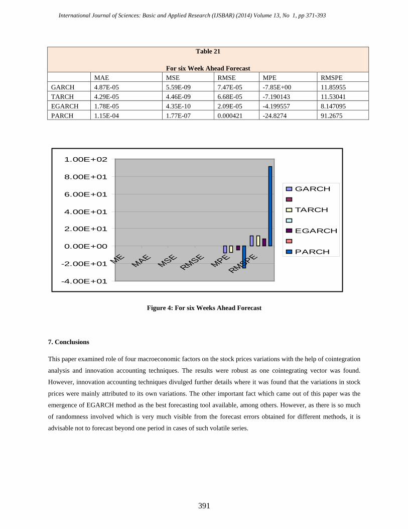
B) Evaluation of methods across different time horizons: The results are presented in tables 19, 20 and 21.The
results are supplemented by figures 2, 3 and 4. Following conclusions could be drawn.
• One dominant result which came out is the emergence of EGARCH as the best forecasting tool available ,
as it has got minimum errors at every time horizons.
389

International Journal of Sciences: Basic and Applied Research (IJSBAR) (2014) Volume 13, No 1, pp 371-393
Table 19
For One Week Ahead Forecast MAE MSE RMSE MPE RMSPE GARCH 4.69E-05 5.30E-09 7.28E-05 -5.170254 7.609951 TARCH 5.07E-05 7.01E-09 8.37E-05 -5.411685 7.946366 EGARCH 3.56E-05 2.84E-09 5.33E-05 -4.561634 7.051415 PARCH 4.34E-05 4.01E-09 6.33E-05 -5.1709 7.521302
-8.00E+00
-6.00E+00
-4.00E+00
-2.00E+00
0.00E+00
2.00E+00
4.00E+00
6.00E+00
8.00E+00
1.00E+01
ME MAE MSE RMSE MPE RMSPE
GARCH
TARCH
EGARCH
PARCH
Figure 2: For One Week Ahead Forecast
Table 20
For three Weeks Ahead Forecast MAE MSE RMSE MPE RMSPE GARCH 4.67E-05 5.29E-09 7.28E-05 -5.80E+00 8.710543 TARCH 4.16E-05 7.57E-09 7.49E-05 -5.501095 8.268005 EGARCH 2.19E-05 8.30E-10 2.88E-05 -3.672351 6.033145 PARCH 3.97E-05 4.31E-05 6.57E-05 -11.17838 35.786
-2.00E+01
-1.00E+01
0.00E+00
1.00E+01
2.00E+01
3.00E+01
4.00E+01
ME MAE MSE RMSE MPE RMSPE
GARCH
TARCH
EGARCH
PARCH
Figure 3: For three Weeks Ahead Forecast
390
International Journal of Sciences: Basic and Applied Research (IJSBAR) (2014) Volume 13, No 1, pp 371-393
Table 21
For six Week Ahead Forecast MAE MSE RMSE MPE RMSPE GARCH 4.87E-05 5.59E-09 7.47E-05 -7.85E+00 11.85955 TARCH 4.29E-05 4.46E-09 6.68E-05 -7.190143 11.53041 EGARCH 1.78E-05 4.35E-10 2.09E-05 -4.199557 8.147095 PARCH 1.15E-04 1.77E-07 0.000421 -24.8274 91.2675
-4.00E+01
-2.00E+01
0.00E+00
2.00E+01
4.00E+01
6.00E+01
8.00E+01
1.00E+02
MEMAE
MSERMSE
MPERMSPE
GARCH
TARCH
EGARCH
PARCH
Figure 4: For six Weeks Ahead Forecast
7. Conclusions
This paper examined role of four macroeconomic factors on the stock prices variations with the help of cointegration
analysis and innovation accounting techniques. The results were robust as one cointegrating vector was found.
However, innovation accounting techniques divulged further details where it was found that the variations in stock
prices were mainly attributed to its own variations. The other important fact which came out of this paper was the
emergence of EGARCH method as the best forecasting tool available, among others. However, as there is so much
of randomness involved which is very much visible from the forecast errors obtained for different methods, it is
advisable not to forecast beyond one period in cases of such volatile series.
391

International Journal of Sciences: Basic and Applied Research (IJSBAR) (2014) Volume 13, No 1, pp 371-393 References:
[1] N. Chen, R. Roll and S. Ross. “Economic Forces and the Stock Market.” Journal of Business, vol. 59, pp. 383-
403, 1986.
[2] Eugene Fama. “ Stock Returns, Real Activity, Inflation and Money.” American Economic Review, vol. 71, pp.
545-565, Sep 1981.
[3] T.K. Mukherjee and A. Naka. “Dynamic Relations between Macroeconomic Variables and the Japanese Stock
Market: An Application of a Vector Error Correction Model.” Journal of Financial Research, vol. 18, No. 2, pp.
223-237, 1995.
[4] R.C. Maysami and T.S Koh. “Vector Error Correction Model of the Singapore Stock Market.” International
Review of Economics and Finance, vol. 9, pp. 79-96, 2000.
[5] B. Solnik. “Using Financial Prices to Test Exchange Rate Models.” Journal of Finance, vol. 42, pp. 141–149,
1987.
[6] H.H.W. Bluhm and J.Yu. “Forecasting Volatility: Evidence from the German Stock market.” Internet:
www.econometricsociety.org/meetings/am01/content/presented/papers/yu.pdf, 2001[Jun21, 2013].
[7] M. Palmquist and B. Viman. “Forecasting volatility in the Swedish stock market; Volatility modeling of the
OMX-index using four different models.”
Internet: www.stat.umu.se/kursweb/vt05/stac05mom3/?download=MatsBjorn.pdf , May 2005[Jul4, 2013].
[8]C. Brooks . “Predicting Stock Index Volatility: Can Market Volume Help?” Journal of forecasting, vol. 17, pp.
59-80, 1998.
[9] M. Karmakar . “Modeling Conditional Volatility of the Indian Stock Markets.” Vikalpa, vol. 30, No.3, 2005.
[10] N. Gospodinov, A. Gavala and D. Jiang. “Forecasting Volatility.” Journal of forecasting, vol. 25, pp. 381-400,
2006.
[11] A. Batra. “ Stock return volatility patterns in India.” Internet: www. icrier.org/pdf/wp124, 2004[Jul5, 2013].
[12] H.R. Badrinath and P.G. Apte. “Volatility Spillovers across Stock, Call Money and Foreign Exchange
Markets.” Internet: www.nse-india.com/content/research/comppaper109.pdf, 2005[Jun20, 2013].
392

International Journal of Sciences: Basic and Applied Research (IJSBAR) (2014) Volume 13, No 1, pp 371-393 [13] G. Goswami and S.C.Jung. “Stock Market and Economic Forces: Evidence from Korea.” Internet:
www.bnet.fordham.edu/public/finance/goswami/korea.pdf, 1997[Jun23, 2013].
[14] A.M. Adam and G.Tweneboah. “Macroeconomic Factors and Stock Market Movement: Evidence from
Ghana.” Internet: www.mpra.ub.uni-muenchen.de/14079/, 2008[Jul3, 2013].
[15] C. Gan, M. lee, H.H.A. Yong and J. Zhang. “Macroeconomic variables and stock market interactions: New
Zealand evidence.” Investment management and financial innovations, vol.3, issue 4, 2006.
[16] A. Humpe and P. Macmillan. “Can macroeconomic variables explain long term stock market movements? A
comparison of the U.S. and Japan.” Internet: www.st-andrews.ac.uk/CDMA/papers/wp0720.pdf, 2007[Jul2, 2013].
[17] N. Günsel and S. Çukur. “The Effects of Macroeconomic Factors on the London Stock Returns: A Sectoral
Approach.” Internet: www.eurojournals.com/irjfe%2010%20nil.pdf, 2007[Jun24, 2013].
[18] R.C. Maysami, L.C. Howe and M.C. Hamzah. “Relationship between Macroeconomic Variables and Stock
Market Indices: cointegration Evidence from Stock Exchange of Singapore’s All-S Sector Indices.” Internet:
www.ukm.my/penerbit/jurnal_pdf/Jp24-03.pdf , 2004[Jun.29, 2013].
[19] S. Johansen. “Estimation and Hypothesis Testing of Cointegration Vectors in Gaussian Vector Autoregressive
Models,” Econometrica, vol. 59, pp.1551- 1580, 1991.
[20] W. Enders. Applied Econometric Time Series. John Wiley & Sons Inc., United States, 1995.
[21]S. Bulmash and G. Trivoli. “Time-lagged interactions between stock prices and selected economic variables.”
The Journal of Portfolio Management (summer), pp. 61–67, 1991.
393