Modeling Ultrasonic Wave Propagation

Through the Kidney

UCSD BENG 221

Fall Project, 2013

Anthony Au, Qin Qin, Norman Huang

Table of Contents

Introduction .................................................................................................................................................. 3

Model ............................................................................................................................................................ 3

Problem Statement: .................................................................................................................................. 3

Assumptions .............................................................................................................................................. 4

Analytical solution ......................................................................................................................................... 4

Numerical Solution ....................................................................................................................................... 8

Conclusions ................................................................................................................................................. 11

Future Works .............................................................................................................................................. 11

References .................................................................................................................................................. 13

Appendix: Matlab code ............................................................................................................................... 14

Introduction

Ultrasound is any sound above the threshold of human hearing (about 20 kHz). For medical applications,

the range for ultrasound is usually between 2 MHz to 20MHz [1]. These waves are mechanical waves,

which are different from electromagnetic waves. This means that the pressure sound waves require a

medium to travel through because the pressure wave travels by displacing particles in the air [2].

Imaging is one of the main applications of ultrasound technology in medicine. It functions similar to

radar technology, where the waves are emitted and reflected back to a receiver. The receiver can then

form an image of the object based on the reflected waves. There are many other medical applications of

ultrasound other than diagnostic imaging. Potential applications include: tissue ablation (cancer),

breaking blood clots (sonothrombolysis), breaking kidney stones (lithotripsy), and promoting healing of

muscle and other tissue [1]. This project focuses on lithotripsy, the breaking of kidney stones with

pulsed ultrasonic waves.

One of the main functions of the kidneys is to remove metabolic products and toxins from blood and

excreting these toxins via urine [3]. A kidney stone is a solid material that forms in the kidney when

there are high concentrations of certain substances present in the urine [4]. Most of these kidney stones

(75%) are comprised of calcium oxalate [5]. The stones may also contain Hydroxyapatite, uric acid or

stuvite [5]. During stone formation, the concentration of calcium oxalate is usually 7 to 11 times its

solubility causing crystals to nucleate [5]. These stones can vary in size, where smaller stones may pass

through the urinary tract with relatively little pain. Larger stones can block the ureter and cause

symptoms ranging from blood in the urine to a sharp pain in the back or lower abdomen area [4].

Current treatments for large kidney stones are uteroscopy, percutaneous nephrolithotomy, and

lithotripsy [4]. Out of the three options, lithotripsy is the only non-invasive method. As hinted earlier,

lithotripsy utilizes ultrasound waves to fragment the stones into smaller pieces that can exit more easily.

The lithotripters create two forces on the stone: a direct force from the shock wave and a force due to

the rapid expansion and collapse of air bubbles [2]. These forces help to break apart the stones, but they

may also cause collateral damage to the surrounding tissues [2]. Little is known about the exact process

by which the stones are fractured and the potential effects of the pressure waves on the body.

Model

Problem Statement: In order to examine the propagation of the sound wave inside of the kidney we will consider a

transducer placed directly against the kidney. The stone is then located on the other side of the kidney

and a sinusoidal input wave is produced by the transducer at the boundary of the kidney. We will begin

with a model of the kidney and stone using the 1D wave equation to track the longitudinal waves

produced by the ultrasound pressure.

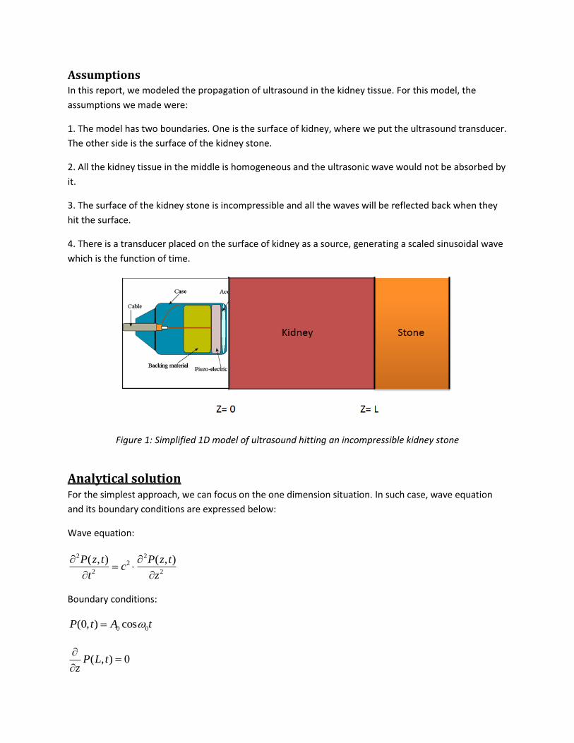
Assumptions In this report, we modeled the propagation of ultrasound in the kidney tissue. For this model, the

assumptions we made were:

1. The model has two boundaries. One is the surface of kidney, where we put the ultrasound transducer.

The other side is the surface of the kidney stone.

2. All the kidney tissue in the middle is homogeneous and the ultrasonic wave would not be absorbed by

it.

3. The surface of the kidney stone is incompressible and all the waves will be reflected back when they

hit the surface.

4. There is a transducer placed on the surface of kidney as a source, generating a scaled sinusoidal wave

which is the function of time.

Figure 1: Simplified 1D model of ultrasound hitting an incompressible kidney stone

Analytical solution For the simplest approach, we can focus on the one dimension situation. In such case, wave equation

and its boundary conditions are expressed below:

Wave equation:

2 22

2 2

( , ) ( , )P z t P z tc

t z

Boundary conditions:

0 0(0, ) cosP t A t

( , ) 0P L tz

In this case, we have a value-flux type boundary condition. The transducer on one side will keep

generating a cosine wave with angular frequency 0 and amplitude 0A . On the other side, the flux is

zero because the surface of the kidney stone is incompressible and reflects all waves without changing

their phases and amplitude.

Because the time-varying component is harmonic oscillator, we can have a solution form like below:

( , ) ( ) j tP z t z e

After applying the separation of variables to the 1D wave equation we get:

22 2

2( )j t j t d

e z c edz

2 2

2 2( ) 0

dz

dz c

Coefficients we are using in this case:

22

2k

c

2 2=

fk

c c

is the angular frequency of the wave propagation, k is wave number here, is the wave length.

22

2( ) 0

dk z

dz

Using characteristic equation to solve this problem:

2 2 0r k

So the eigenvalues are

1,2r j k

Thus the solution to (1) is:

( ) jkz jkzz A e B e

Then we have our general solution to the one dimension wave equation:

( , ) ( ) ( )j t jkz jkz j tP z t z e A e B e e

To solve A and B, we apply BCs :

0(0, ) ( ) cosj tP t A B e t

( , ) ( ) 0j t jkL jkLP L t jk e A e B ez

Since j tjk e cannot be zero, then

0jkL jkLA e B e 2j kLA B e

0( ) cosj tA B e t 0 0 0 0( ) ( )

2 2

j t j t j t j t

j t

e e e eA B

e

Finally we get:

0 0( ) ( )

22(1 )

j t j t

j kL

e eA

e

0 0( ) ( )

22(1 )

j t j t

j kL

e eB

e

A and B are both the functions of time.

The analytical solution is:

0 0 0 0( ) ( ) ( ) ( )

2 2( , ) ( )

2(1 ) 2(1 )

j t j t j t j tjkz jkz j t

j kL j kL

e e e eP z t e e e

e e

After simplifying , the imaginary parts are eliminated resulting in the following:

0

cos( ) cos( ( 2 ))( , ) ( ) cos( )

1 cos(2 )

kz k z LP z t t

kL

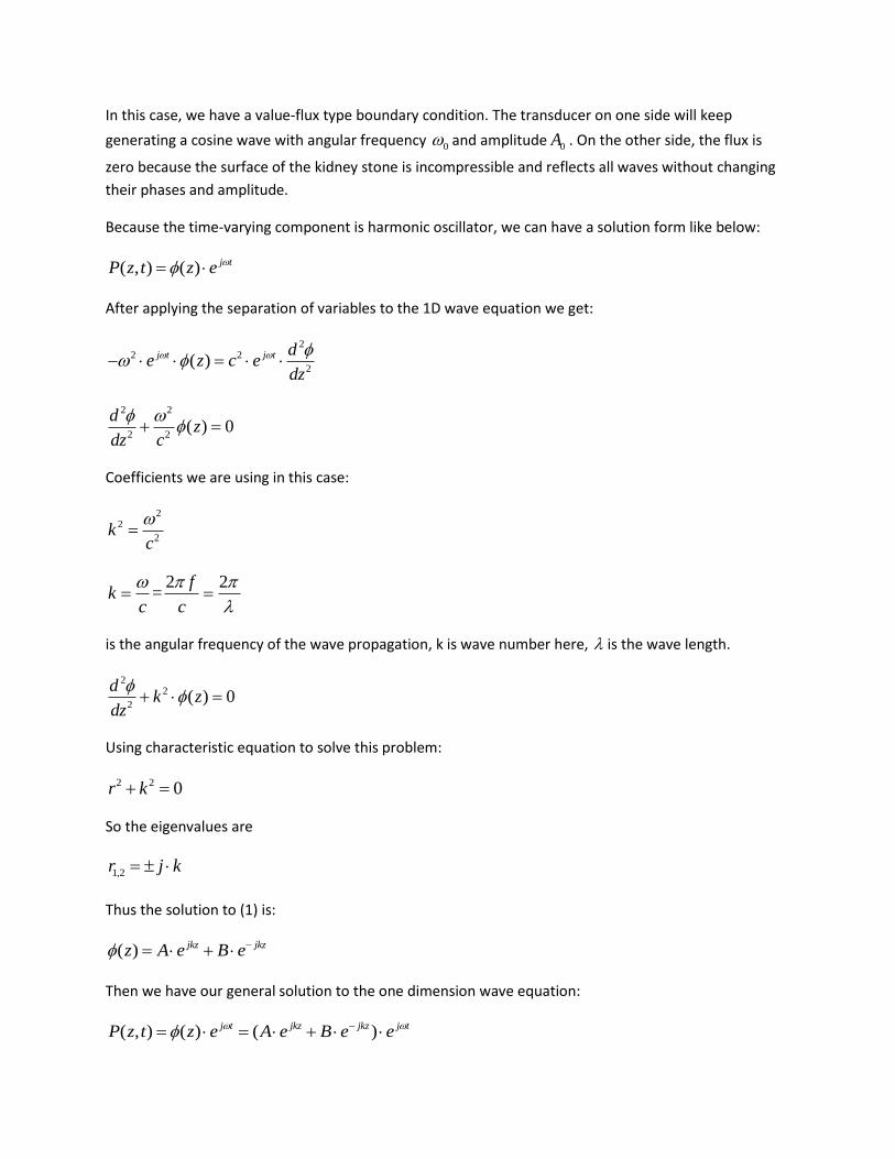
Figure 2: plot of our analytical solution in time and space

Figure 2 shows a plot of the analytical solution. It shows the cosine wave over time on the time axis. This

follows our boundary condition of cos(w0t). There are cosine waves in the space direction, which is what

the analytical solution predicted (combination of cosine waves). Therefore, since the time and space

axes are both cosine waves, a matrix of cosine waves is created. Basically, the transducer sends a

different starting pressure at each time point. This means that a cosine wave will propagate in the

kidney slightly out of phase until it eventually becomes in phase again. These results are as expected,

but they are not very interesting, since the entire wave is reflected back at the end boundary. This

means that there is no amplitude attenuation or phase change, which shows in the plot. If there was a

phase change, the back propagating wave would interfere with the forward propagating wave and result

in a wave with a lower amplitude (possibly 0 if anti-phase). The pressure amplitude will scale with the

input transducer wave. If we input a wave with higher amplitude, the amplitude of the solution will scale

proportionally.

0

50

100

150

0

1

2

3

4

5

-2

0

2

time(ns)

High Frequency Sound Wave

space(cm)

Pre

ssure

(Pa

)

Numerical Solution For our numerical solution, we utilized the PDE toolbox, which calculates finite elements approximations

to solve PDEs in 2D defined in a bounded plane. After defining the boundaries on a 2D plane, the space

is broken up into smaller geometric domains, which in this case is a triangular mesh, which is assumed

to be continuous.

After breaking the boundaries into meshes, the solution for each bound is calculated based on the PDE,

which in our case is hyperbolic. The solution is then plotted in respect to time.

2D to 1D solution Comparison:

We wanted to compare our results for a 20MHz from our 1D analytical solution with the 2D numerical

solution to see if the behavior was similar.

Our results showed that after a long time, the individual waves are reflected and form larger waves with

the newly generated input waves. This does align with our 1D solution which shows uniform waves

initially at .15 milliseconds.

Figure 3:

Figure 4: 2D wave model, 20 MHz cos wave generated at the top boundary and zero flux

through the bottom boundary to model kidney stone layer. Time is in milliseconds.

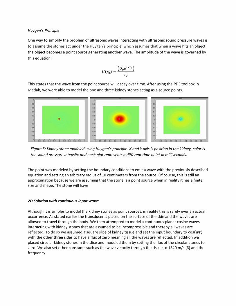
Huygen’s Principle:

One way to simplify the problem of ultrasonic waves interacting with ultrasonic sound pressure waves is

to assume the stones act under the Huygen’s principle, which assumes that when a wave hits an object,

the object becomes a point source generating another wave. The amplitude of the wave is governed by

this equation:

( ) (

)

This states that the wave from the point source will decay over time. After using the PDE toolbox in

Matlab, we were able to model the one and three kidney stones acting as a source points.

The point was modeled by setting the boundary conditions to emit a wave with the previously described equation and setting an arbitrary radius of 10 centimeters from the source. Of course, this is still an approximation because we are assuming that the stone is a point source when in reality it has a finite size and shape. The stone will have 2D Solution with continuous input wave: Although it is simpler to model the kidney stones as point sources, in reality this is rarely ever an actual occurrence. As stated earlier the transducer is placed on the surface of the skin and the waves are allowed to travel through the body. We then attempted to model a continuous planar cosine waves interacting with kidney stones that are assumed to be incompressible and thereby all waves are reflected. To do so we assumed a square slice of kidney tissue and set the input boundary to ( ) with the other three sides to have a flux of zero meaning all the waves are reflected. In addition we placed circular kidney stones in the slice and modeled them by setting the flux of the circular stones to zero. We also set other constants such as the wave velocity through the tissue to 1540 m/s [6] and the frequency.

Figure 5: Kidney stone modeled using Huygen’s principle. X and Y axis is position in the kidney, color is

the sound pressure intensity and each plot represents a different time point in milliseconds.

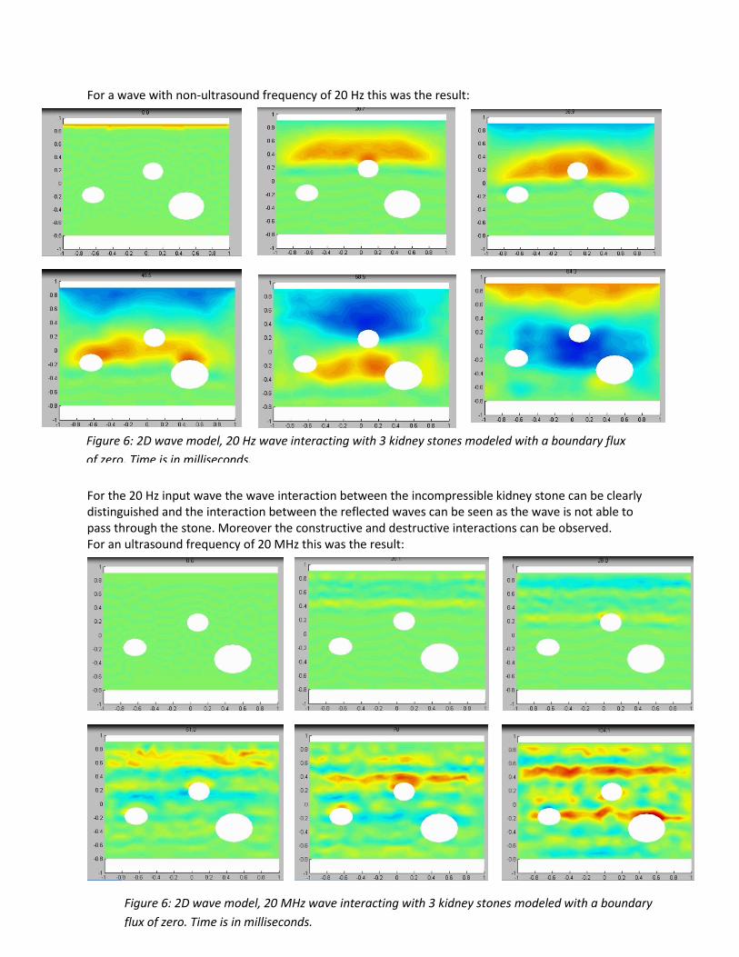
For a wave with non-ultrasound frequency of 20 Hz this was the result:

For the 20 Hz input wave the wave interaction between the incompressible kidney stone can be clearly distinguished and the interaction between the reflected waves can be seen as the wave is not able to pass through the stone. Moreover the constructive and destructive interactions can be observed. For an ultrasound frequency of 20 MHz this was the result:

Figure 6: 2D wave model, 20 Hz wave interacting with 3 kidney stones modeled with a boundary flux

of zero. Time is in milliseconds.

Figure 6: 2D wave model, 20 MHz wave interacting with 3 kidney stones modeled with a boundary

flux of zero. Time is in milliseconds.

Since the frequency is higher, the period of oscillations should be shorter which appears in the model. One interesting behavior is the eventual constructive waves that are formed, which might be explained as a small phase shift in a period could form a wave with larger amplitude. Overall, our model appears to show that ultrasound frequencies do apply a large amplitude sound wave onto kidney stones as the treatment continues in the body.

Conclusions

Our analytical model served to demonstrate a wave propagating through a homogenous 1 dimensional

tissue in response to a sinusoidal input. This gave a better understanding of the complex interactions

that may occur within the kidney by first understanding the basic propagation of the wave in 1d space

and time. We further complicated our system in the numerical model to closer approach the

physiological situation. The system was still only a 2D system, but it showed how the wave became

distorted when it encountered the zero flux holes, which represented the stones. With a time lapse

video, we were able to see the pressure changes in the system. The reflected waves interacted with

each other, causing both destructive and constructive interference that were capable of producing large

pressures.

Future Works

This model was an extremely simplified version of the actual problem. In reality, the problem takes place

in a 3 dimensional system, where the reflected waves can move with several degrees of freedom. In the

future, we would like to apply the wave equation using 3d spherical coordinates. In addition, kidney

stones are not circular discs or even perfect spheres. They come in a variety of shapes ranging from

smooth spherical or elliptical to jagged polygons. Most likely a finite element or finite difference

approach will be needed in order to accurately account for these non-symmetric shapes.

In the analytical and numerical analyses, we used homogeneous boundary conditions for the stone (e.g.

zero flux). A more realistic boundary condition would be a mix of value and flux. For example a boundary

condition such as ( )

( ) . This boundary means that there will be some wave reflected

ad some wave absorbed, which is what would happen to the stone and surrounding tissue since there is

no such material that is perfectly incompressible. In the future, for our other boundary condition,

instead of a sinusoidal wave, we could use a pulsed pressure wave. Generally, most lithotripsy

transducers generate a large pulse of pressure and focus it into the kidney.

Last of all, we would like to expand our model to examine the forces and stresses applied to both the

kidney and stone. This has the largest practical implications as it relates directly with patient safety and

the efficiency of the shockwaves in splitting the kidney stones. Once the exact mechanism for the stone

fragmentation is known, the process can be streamlined to focus the waves to produced only the

desired effect and minimize collateral damage to the tissue.

References

[1] A. Carovac, F. Smajlovic, D. Junuzovic. (2011, Sep.). “Application of Ultrasound in Medicine.” Acta

Inform Med. [Online]. 19(3), pp. 168-171. Available:

http://www.ncbi.nlm.nih.gov/pmc/articles/PMC3564184/

[2] A.D. Smith, R.O. Cleveland, J.A. McAteer. “The Physics of Shock Wave Lithotripsy,” in Smith’s

Textbook of Endourology, 3rd ed., Wiley-Blackwell, 2012, pp. 317-332.

[3] W. F. Boron, E. L. Boulpaep, “Organization of the Urinary System,” in Medical Physiology, 2nd ed.

Philadelphia: Saunders Elsevier, 2009, pp. 749-850.

[4] “What I need to know about Kidney Stones.” Internet:

http://kidney.niddk.nih.gov/kudiseases/pubs/stones_ez/#kidneystone, July 24, 2013[Nov. 30, 2013].

[5] F. L. Coe, J. H. Parks, J. R. Asplin. (1992, Oct.). “The Pathogenesis and Treatment of Kidney Stones.”

N Engl J Med. [Online]. 327(15), pp. 1141-1152. Available:

http://www.nejm.org/doi/pdf/10.1056/NEJM199210153271607[Nov. 30, 2013].

[6] Narouze, Samer N.. <i>Atlas of ultrasound-guided procedures in interventional pain

management</i>. New York: Springer, 2011. Print.

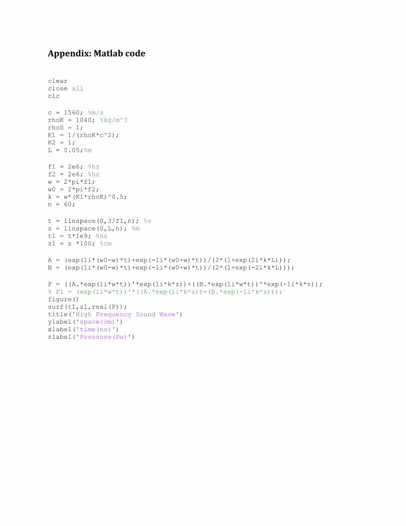
Appendix: Matlab code

clear close all clc

c = 1560; %m/s rhoK = 1040; %kg/m^3 rhoS = 1; K1 = 1/(rhoK*c^2); K2 = 1; L = 0.05;%m

f1 = 2e6; %hz f2 = 2e6; %hz w = 2*pi*f1; w0 = 2*pi*f2; k = w*(K1*rhoK)^0.5; n = 60;

t = linspace(0,3/f1,n); %s z = linspace(0,L,n); %m t1 = t*1e9; %ns z1 = z *100; %cm

A = (exp(1i*(w0-w)*t)+exp(-1i*(w0+w)*t))/(2*(1+exp(2i*k*L))); B = (exp(1i*(w0-w)*t)+exp(-1i*(w0+w)*t))/(2*(1+exp(-2i*k*L)));

P = ((A.*exp(1i*w*t))'*exp(1i*k*z))+((B.*exp(1i*w*t))'*exp(-1i*k*z)); % P1 = (exp(1i*w*t))'*((A.*exp(1i*k*z))+(B.*exp(-1i*k*z))); figure() surf(t1,z1,real(P)); title('High Frequency Sound Wave') ylabel('space(cm)') xlabel('time(ns)') zlabel('Pressure(Pa)')