Modeling Two Stock Prices using Diffusion Process

BENIN JOURNAL OFSTATISTICS

ISSN 2682-5767Vol. 3, pp. 116– 127 (2020)

Modeling Two Stock Prices using Diffusion Process

A. H. Ekong1∗, O. E. Asiribo2 and S. Okeji3

1,2,3Department of Statistics, Federal University of Agriculture Abeokuta, Ogun State, Nigeria

Abstract. In real life applications, the parameters of a stochastic differential equation (SDE) are unknown and needto be estimated. In most cases what is available is only sampled data of the process at discrete times. It is a commonpractice to use the discretization of the original continuous time process for the modeling. SDEs have solutions incontinuous-time called diffusion process. The methodology as applied to stock price involves a discrete time stochasticmodel for the dynamical system under study. For a small time interval, ∆t, the possible changes with their corre-sponding transition probabilities are determined. The expected change and the covariance matrix for the change aredetermined for the discrete time stochastic process. The system of SDEs is obtained by letting the expected changedivided by ∆t,- be the drift coefficient and the square root of the covariance matrix divided by ∆t,- be the diffusioncoefficient. The SDE model is inferred by similarities in the forward Kolmogorov equations between the discrete andthe continuous stochastic processes. The resulting SDE model with estimated drift and volatility parameters is solvedusing the multi-dimensional Euler-Maruyama scheme for SDEs as implemented using the R packages ’Sim.DiffProc’and ’yuima’.

Keywords: Markov process, stochastic differential equation, transition probabilities, diffusion process, dynamical system, drift,volatility.

Published by: Department of Statistics, University of Benin, Nigeria

1. Introduction

A dynamical system is a system that describes the time dependence of a point in a geometrical space. Exam-ples of such a system include traffic at a particular street light, the price of equities and stocks, the number ofvehicles arriving at a filling station for fuel over a period, etc. Dynamical systems can be represented by therules of evolution that describe the future state of the system from the current state. A dynamical system canbe deterministic if only one future state is determined by the current state of the system or stochastic whenfuture state is determined by random events or states. Most physical processes in the real world involve arandom element in their structure. Thus a stochastic process can be described as a statistical phenomenonthat evolves in time according to probabilistic laws (Chatfield, 2004).

Dynamical systems are usually described using differential equations which give the time derivatives forthe system. Ordinary differential equations are used for system in finite dimensional space, but there are ex-tensions to infinite-dimensional space, in which case the differential equations are partial differential equa-tions. Dynamical system perspective to partial differential equations has begun to gain popularity. Unlikedeterministic models that are based on ordinary differential equations, with a unique solution for each appro-priate initial condition, stochastic differential equations (SDEs) have solutions that are in continuous-time. Amajor motivation for SDEs in modeling real world dynamical systems is that there is a nonlinear dependenceof the level of the series on previous data points (Allen, 2007).

Casdagli (1991), in his work on forecasting algorithm, attempts to ”bridge the gap” between the stochas-tic and deterministic approaches were made. The forecasting algorithm was applied to a variety of exper-imental and naturally occurring time series data, with a view to investigating whether a dataset exhibitslow-dimensional chaotic behaviour, as opposed to high-dimensional or stochastic behaviour.

Tiberio (2004) noted that the change in a system could be done from a stochastic or deterministic perspec-tive. Models based on deterministic differential equation are more likely to be implemented by sociologists

∗Corresponding author. Email: [email protected]

http://www.srg-uniben.org/

117 Ekong et al.

and psychologists, whereas models based on stochastic differential equation are more regularly implementedby econometricians (Tiberio, 2004).

In mathematical finance traditional models are based on stochastic processes which are variables thatevolve over time in a way that is at least in part random. Prices of financial assets are believed to have arandom behavior fully or partly with some known mathematical and distributional properties. Stochastic be-havior is usually driven by Brownian motion (or Wiener process). Brownian motion is a Markovian stochasticprocess with independent, stationary and normally distributed increments (McNicholas et al., 2012).

Wang (2015) examined dynamical models of stock prices based on technical trading rules, referred toas the moving average rules. The work showed that the price dynamical model has an infinite number ofequilibriums, but all these equilibriums were unstable and that although the price was chaotic, the volatilityconverged to some constant very quickly at the rate of the Lyapunov exponent.

The chaotic nature of stock prices as revealed by Wang (2015) makes it crucial in examining the modelsused to fit stocks prices. Damptey (2017) looked at the appropriateness of the Geometric Brownian motionmodel for forecasting stock prices by comparing simulated data sets with market prices of some companies.The findings showed that the Geometric Brownian Motion (GBM) model is a more appropriate model forforecasting stock prices on the Ghana stock exchange.

Reddy and Clinton (2016) examined the evidence of simulating stock price using Geometric BrownianMotion from Australian companies. The results showed that over all time horizons the chances of a stockprice simulated using GBM moving in the same direction as real stock prices was a little greater than 50percent.

Reddy and Clinton (2016) noted that the correlation coefficient between simulated stock prices and actualstock prices, mean absolute percentage error and directional movements of simulated and actual stock pricesmay be used to test the validity of the model.

Maruddani and Trimono (2018) expanded the GBM model to carter for portfolio of stocks by using mul-tidimensional GBM and they reported that the model gave a less mean absolute percentage error than that ofGBM for single stock. They simulated stock price from the Indonesian Exchange (IDX) Top Ten Blue 2016for two companies and reported the mean absolute percentage error value was less than 10% in favour of themultidimensional GBM. This means that the method is highly accurate for the model.

With the findings of Wang (2015) about the chaotic behavior of stock prices and the Markov property ofSDE which lends itself to the concept of short term predictability of chaotic systems, this becomes a moti-vation to examine diffusion process in modeling a dynamical system (stock prices) using discrete stochasticdifferential equations for the modeling process. Hence, the main aim of the study is to model the dynamicsof two stock prices using a stochastic differential equation of the Ito type, given the discrete-time realisa-tions from the process. Even though the study considered a continuous-time process (stock price), the stackreality is that realizations from the continuous-time processes are taken in discrete times. So the approach isto describe the continuous-time process using the discrete-time observations

2. Materials and method

2.1 Chapman Kolmogorov formula

For discrete time stochastic processes with τ = (t0, t1, t2, . . . ) defining a set of discrete times andX(t0), X(t1), X(t2), ... defining the sequence of random variables each on the sample space Ω. This systemmay describe, for instance the evolution of stock price over the discrete times t0, t1, t2, . . . . This study relieson the Markov property that the present value of a random variable X(tn) only determines the future valueX(tn+1) and such systems (Xn), are said to be Markov processes. Markov processes are usually useful indeveloping the SDE models for biological and financial systems, the latter of which this study focuses on.

Given the time interval ∆t = 1/N , for ti = i∆t, i = 0, 1, 2, . . . , N and Xi = X(ti) with X0 = 0,there is a discrete random variable δ, that takes on values −β, 0, β, representing nominal values definingthe movement of the variable X(tn) at any time tn+1. For the stock price, the nominal values −β, 0, β,represents a loss, no change or a gain in stock price at tn+1.

One property of the Markov process is the relation known as the Chapman-Kolmogorov formula

p(l+n)i,j =

∞∑m=0

p(l)i,mp

(n)m,j ∀ l, n ≥ 0


Modeling two stock prices... 118

where pi,j = P (Xn+1 = j | Xn = i) i ≥ 0, j ≥ 0 defines the transition probabilities for discrete timestn = n∆t so that tn+k = tn + tk (Allen, 2007).

This property for a discrete stochastic process is contained in the forward Kolmogorov equation which isof interest in developing models with stochastic differential equation herein as described by Allen (2007).Let ti = i∆t for i = 0, 1, . . . , N and let xj = jδ, for j = ...,−2,−1, 0, 1, 2, . . . . Let X0 be given. Definethe transition probabilities of the discrete random variable δ representing the change in the discrete-timestochastic process Xn per time by the following:

r(t, xi)∆tδ2 , for k = i+ 1

pi,k(t) = 1− r(t, xi)∆tδ2 − s(t, xi)

∆tδ2 , for k = i

s(t, xi)∆tδ2 , for k = i− 1

where r and s are smooth nonnegative functions. If ∆X is the change in the stochastic process at time t fixingX(t) = xi, then the mean changeE(∆X) = (r(t,X)−s(t,X))/∆t/δ and variance in change V ar(∆X) =(r(t,X)−s(t,X))∆t. It is assumed that ∆t/δ2 is so small that 1−r(t, xi)∆t/δ2−s(t, xi)∆t/δ2 is positive.Let pk(t) = P (X(t) = xk) be the probability distribution at time t. Then, pk(t+ ∆t) satisfies

pk(t+ ∆t) = pk(t) + [pk+1(t)s(t, xk+1)− pk(t)(r(t, xk) + s(t, xk))+pk−1(t)r(t, xk−1)]∆t/δ2 (1)

As ∆t → 0, the discrete stochastic process approaches a continuous-time process. As ∆t → 0, pk(t)satisfies the initial-value problem:

dpk(t)dt = −

(pk+1(t)a(t,xk+1)−pk−1(t)a(t,xk−1)

2δ

)+

(pk+1(t)b(t,xk+1)−2pk(t)b(t,xk)+pk−1(t)b(t,xk−1)

2δ2

)(2)

for k = ...,−2,−1, 0, 1, 2, . . . and (pk(0))mk=−m are known. Equation (2) is the forward Kolmogorov equa-tion for the continuous-time stochastic process which approximates the partial differential equation

∂p(t, x)

∂t= −∂(a(t, x)p(t, x))

∂x+

1

2

∂2(b(t, x)p(t, x))

∂x2(3)

and corresponds to a diffusion process having the stochastic differential equation

dX(t) = a(t,X)dt+√b(t,X)dW (t) (4)

An in-depth presentation of this process can be found in Allen (2007).There exists a relationship between the discrete stochastic process defined by (3) and the continuous pro-

cess defined by (4). For small ∆t and δ, the probability distribution of the solution to (4) will be approxi-mately the same as the probability distribution of solutions to the discrete stochastic process (Allen, 2007). Arealistic discrete stochastic process model for the dynamical system under investigation in this study can thusbe constructed by developing a discrete stochastic differential equation model. As time is made continuous(for small ∆t and δ), then the solution of the stochastic differential equation approximates the dynamicalsystem under study.

2.2 Diffusion process model for stock price

It is important to note that certain assumptions are made here in the derivation of the model for stock pricesand these include:

• The process for stock price is stochastic rather than deterministic and a finite ∆t produces a discretestochastic model.• The form assumed for the probabilities of the possible price changes over a small time step is that

the probability of a change in one stock price is proportional to the stock price.


119 Ekong et al.

• For a simultaneous change in both stock prices, it is assumed that the probability of the change isproportional to the product of the two stock prices.• The time interval ∆t is sufficiently short such that the probability of more than one change in the

stock prices is small and the probability that change in both stocks is zero is positive.• Large jumps in stock prices caused by sudden major changes in the financial environment are not

considered in this model development.

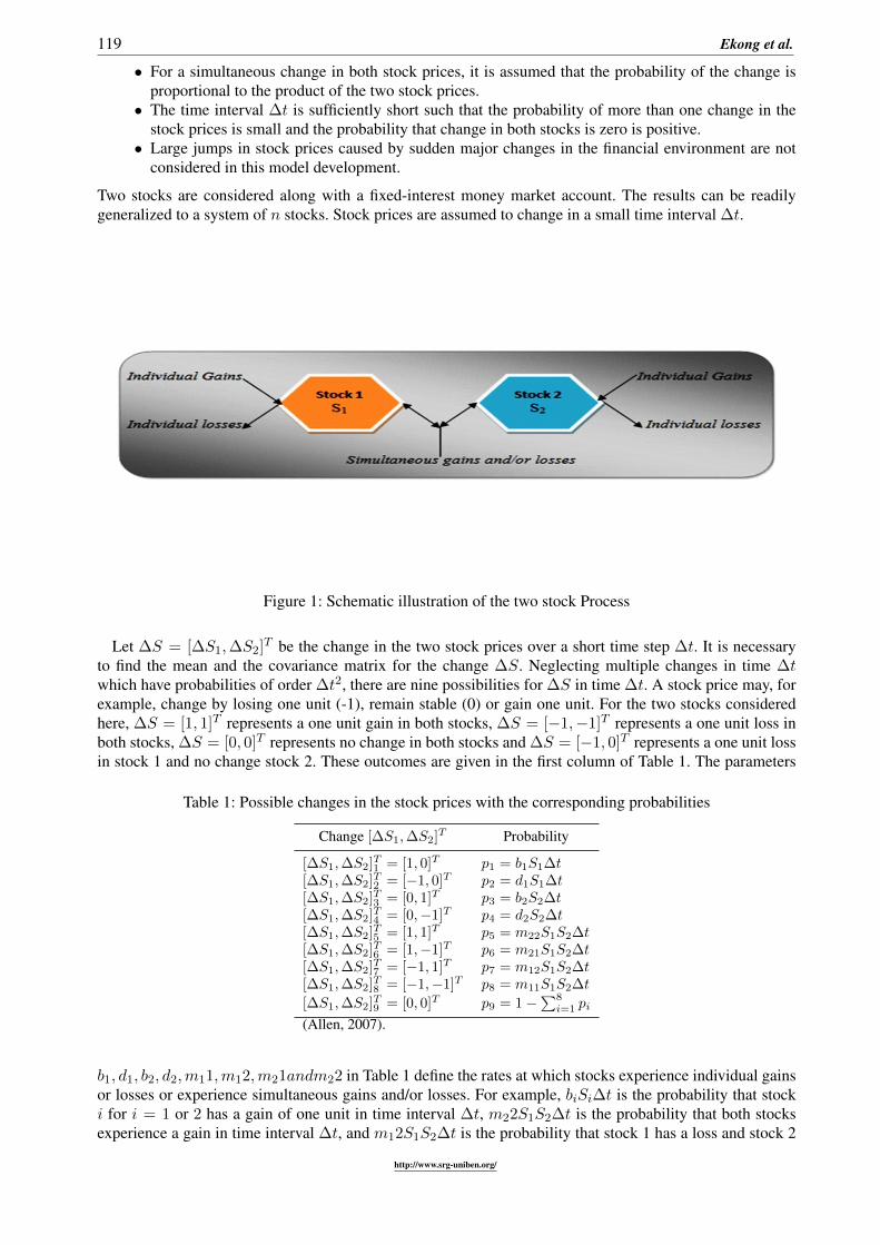
Two stocks are considered along with a fixed-interest money market account. The results can be readilygeneralized to a system of n stocks. Stock prices are assumed to change in a small time interval ∆t.

Figure 1: Schematic illustration of the two stock Process

Let ∆S = [∆S1,∆S2]T be the change in the two stock prices over a short time step ∆t. It is necessaryto find the mean and the covariance matrix for the change ∆S. Neglecting multiple changes in time ∆twhich have probabilities of order ∆t2, there are nine possibilities for ∆S in time ∆t. A stock price may, forexample, change by losing one unit (-1), remain stable (0) or gain one unit. For the two stocks consideredhere, ∆S = [1, 1]T represents a one unit gain in both stocks, ∆S = [−1,−1]T represents a one unit loss inboth stocks, ∆S = [0, 0]T represents no change in both stocks and ∆S = [−1, 0]T represents a one unit lossin stock 1 and no change stock 2. These outcomes are given in the first column of Table 1. The parameters

Table 1: Possible changes in the stock prices with the corresponding probabilities

Change [∆S1,∆S2]T Probability

[∆S1,∆S2]T1 = [1, 0]T p1 = b1S1∆t[∆S1,∆S2]T2 = [−1, 0]T p2 = d1S1∆t[∆S1,∆S2]T3 = [0, 1]T p3 = b2S2∆t[∆S1,∆S2]T4 = [0,−1]T p4 = d2S2∆t[∆S1,∆S2]T5 = [1, 1]T p5 = m22S1S2∆t[∆S1,∆S2]T6 = [1,−1]T p6 = m21S1S2∆t[∆S1,∆S2]T7 = [−1, 1]T p7 = m12S1S2∆t[∆S1,∆S2]T8 = [−1,−1]T p8 = m11S1S2∆t

[∆S1,∆S2]T9 = [0, 0]T p9 = 1−∑8

i=1 pi

(Allen, 2007).

b1, d1, b2, d2,m11,m12,m21andm22 in Table 1 define the rates at which stocks experience individual gainsor losses or experience simultaneous gains and/or losses. For example, biSi∆t is the probability that stocki for i = 1 or 2 has a gain of one unit in time interval ∆t, m22S1S2∆t is the probability that both stocksexperience a gain in time interval ∆t, and m12S1S2∆t is the probability that stock 1 has a loss and stock 2



has a gain in time interval ∆t. These probabilities given in second column of Table 1 are defined as the ratioof the frequency of change ∆S and the total number of observations N , for instance,

p1 = b1 =Numberoftimes[1, 0]Twasobserved

Totalnumberofobservations

and

p5 = m22 =Numberoftimes[1, 1]Twasobserved

Totalnumberofobservations

Using the above expressions for pi and ∆Si, the expectation vector and the covariance matrix for the change∆S can be derived as follows. Neglecting the terms of order (∆t)2, it follows that

E(∆S) =∑9

j=1 pj [∆S1,∆S2]T = b1

(10

)S1 + d1

(−10

)S1 + b2

(01

)S2

+ d2

(0−1

)S2 +m22

(11

)S1S2 +m21

(1−1

)S1S2 +m12

(−11

)S1S2

+m11

(−1−1

)S1S2 +m00

(00

)S1S2

=

(b10

)S1 +

(−d1

0

)S1 +

(0b2

)S2 +

(0−d2

)S2 +

(m22

m22

)S1S2

+

(m21

−m21

)S1S2 +

(−m12

m12

)S1S2 +

(−m11

−m11

)S1S2 +

(00

)S1S2

=

((b1 − d1)S1 + (m22 +m21 −m12 −m11)S1S2

(b2 − d2)S2 + (m22 −m21 +m12 +m11)S1S2

)

E(∆S) = µ(t, S1, S2)∆t

and

E(∆S(∆S)T )) =∑9

j=1 pj∆Sj(∆Sj)T =

[c1 + c2 + c3 c2 − c3

c2 − c3 c2 + c3 + c4

]∆t

V (t, S1, S2)∆t

where c1 = (b1 + d1)S1, c2 = (m22 + m11)S1S2, c3 = (m21 + m12)S1S2, and c4 = (b2 + d2)S2. As theproduct E(∆S)(E(∆S))T is of order (∆t)2, the covariance matrix V is set to equal to E(∆S(∆S)T )/∆t(Allen, 2007).

Now V is positive definite and hence has a positive definite square root. Let B = (V )1/2, as ∆t→ 0, theprobability distribution of the stock prices approximates the probability distribution of solutions to the Ito


121 Ekong et al.

stochastic differential equation system (Allen, 2007):

dS(t) = µ(t, S1, S2)dt+B(t, S1, S1)dW (t) (5)

with S(0) = S0 and whereW (t) is the two-dimensional Wiener processW (t) = [W1(t),W2(t)]T . Equation(5) is a system of stochastic differential equations that describe the dynamics of the stock prices with

µ(t, S1, S2) =

[(b1 − d1)S1 + (m22 +m21 −m12 −m11)S1S2

(b2 − d2)S2 + (m22 −m21 +m12 +m11)S1S2

](6)

with c1 = (b1 + d1)S1, c2 = (m22 +m11)S1S2, c3 = (m21 +m12)S1S2, c4 = (b2 + d2)S2 and

B(t, S1, S2) = 1d

[c1 + c2 + c3 + w c2 − c3

c2 − c3 c2 + c3 + c4 + w

](7)

where w =√

(c1 + c2 + c3)(c2 + c3 + c4)(c2 − c3)2 andd =√c1 + 2c2 + 2c3 + c4 + 2w.

As Allen (2007) noted, the standard geometric Brownian motion model has its drift and diffusion coef-ficients proportional to the stock price. The drift and diffusion coefficients for a single stock of the modelhere, on the other hand, is a linear function of the stock price and similar to an affine model as described inChernov et al., (2003).

3. Results and discussion

3.1 Data description and visualisation

In other to characterize the drift and volatility which will form the coefficients of the stochastic differentialequations, the daily stock prices of two selected stocks Coca-cola and Pepsi for the period of 2009-07-06 to2019-07-05 were collected from Yahoo Finance Online, for the modeling process.

Figure 2 shows the plot of the stock price dataset for Coca-cola and Pepsi. Figure 2-A shows the plot of thestocks of Pepsi and Figure 2-B shows the plot of the stocks of Coca-cola for the period the data was observed.From these plots it can be observed that the stock prices of Pepsi within the period is above the stock priceof Coca-cola and both stocks have appreciated significantly within the period. However, further analysis ofthe stocks and modeling will give details not obvious from these two plots (Figure 2-A and Figure 2-B).Figure 2-C shows the plot of both stocks and the difference observed can be attributed to the fact that, whileabsolute price is important (pricey stocks are difficult to purchase, which affects not only their volatility butthe ability to trade that stock), when trading, more concern is on the relative change of an asset rather thanits absolute price. Pepsi’s stocks from the dataset are more expensive than Coca-cola’s stocks in terms oftheir stock prices on stock exchange, but not on consumer prices in the market and this difference makesCoca-cola’s stocks appear much less volatile than they truly are (that is, their price appears to not deviatemuch as can be seen in Figure 2-C).

One solution would be to use two different scales when plotting the data; one scale will be used by Coca-cola stocks and the other by Pepsi stocks. This results in the plot in Figure 2-D, but sometimes this solu-tion can be difficult to implement well and it can lead to misinterpretation, and may not be read easily. Atransformation the data into a more useful format may give better information than already obtained. Onetransformation would be to consider the stocks’ return since the beginning of the period of interest, that is,to plot the returns defined as:

returnt,0 =pricetprice0

As the interest in this study is in the change of the stocks per day, a plot of this change will also be madeby plotting the log-difference of the stocks, which can be interpreted as the percentage change in a stock but



Jul 06 2009 Jan 02 2013 Jan 03 2017

A 2009−07−06 / 2019−07−05

60

80

100

120

60

80

100

120

Jul 06 2009 Jan 02 2013 Jan 03 2017

B 2009−07−06 / 2019−07−05

25

30

35

40

45

50

25

30

35

40

45

50

2010 2012 2014 2016 2018

2060

100

Date

Pric

e

C

Coca−colaPepsi

2010 2012 2014 2016 2018

6080

100

120

Date

Pric

e

D

2535

45

PepsiCoca−cola

Figure 2: Various Plots of Stock Prices of Coca-cola and Pepsi

does not depend on the denominator of a fraction, when comparing day t to day t+ 1, with the formula:

changet = lg(pricet+1)− lg(pricet)

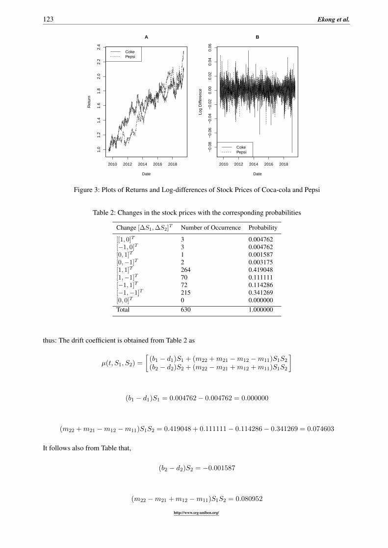
Figure 3 shows the plots of the returns and log-differences of both stock prices. From Figure 3-A, the prof-itability of each stock since the beginning of the period can be seen. The stocks of Coca-cola was moreprofitable than the stock of Pepsi between the period 2011 and 2014, but the stock of Coca-cola droppedbelow the stocks of Pepsi between 2017 and the end of the period 2019 as the stocks of Pepsi was moreprofitable. This trend can be further seen in the log-difference plot as from the beginning of the period thelog-difference of the daily change in Pepsi stock were higher than those of Coca-cola stock and vice versa.Furthermore, it can be seen that these stocks are correlated; they generally move in the same direction, a factthat was difficult to see in Figure 2-C.

3.2 Stochastic differential modeling of Coca-Cola and Pepsi stocks data

The data from 3/01/2017 to 5/07/2019 for stocks of Coca-cola (S1) and Pepsi (S2) for 630 days period wereused for the modeling. The corresponding transition probabilities are given in Table 2, which also shows thedaily simultaneous change in S1 and S2. The methodology described in Section 2.2 is applied to the set ofdata for both stock prices to model the stochastic process. The second column in Table 2 shows the frequencyof each possible simultaneous change in both stocks.

The procedure involved for obtaining the number of occurrence was that the prices of both stocks for thefuture day t + 1, were compared with the prices of the current day t, and if a stock gained in price, thenominal values 1, was taken if a stock lost in price, -1 was noted and if the price was unchanged, 0 wasrecorded. This process is repeated for both stocks each day from day number 1 to number 630. At the end,the number of occurrence for each of the nine possible changes for both stocks is recorded as given in thesecond column of Table 2, out of the total of 630 days. The probability column of Table 2 is as defined inSection 2.2 and is the relative frequency of the number of occurrence and the total number of periods theobservations were taken (630). From Table 2, the parameters of drift coefficient and volatility are computed


123 Ekong et al.

2010 2012 2014 2016 2018

1.0

1.2

1.4

1.6

1.8

2.0

2.2

2.4

Date

Ret

urn

A

CokePepsi

2010 2012 2014 2016 2018

−0.

08−

0.06

−0.

04−

0.02

0.00

0.02

0.04

0.06

Date

Log

Diff

eren

ce

B

CokePepsi

Figure 3: Plots of Returns and Log-differences of Stock Prices of Coca-cola and Pepsi

Table 2: Changes in the stock prices with the corresponding probabilities

Change [∆S1,∆S2]T Number of Occurrence Probability

[[1, 0]T 3 0.004762[−1, 0]T 3 0.004762[0, 1]T 1 0.001587[0,−1]T 2 0.003175[1, 1]T 264 0.419048[1,−1]T 70 0.111111[−1, 1]T 72 0.114286[−1,−1]T 215 0.341269[0, 0]T 0 0.000000Total 630 1.000000

thus: The drift coefficient is obtained from Table 2 as

µ(t, S1, S2) =

[(b1 − d1)S1 + (m22 +m21 −m12 −m11)S1S2

(b2 − d2)S2 + (m22 −m21 +m12 +m11)S1S2

]

(b1 − d1)S1 = 0.004762− 0.004762 = 0.000000

(m22 +m21 −m12 −m11)S1S2 = 0.419048 + 0.111111− 0.114286− 0.341269 = 0.074603

It follows also from Table that,

(b2 − d2)S2 = −0.001587

(m22 −m21 +m12 −m11)S1S2 = 0.080952



Therefore, we have

µ(t, S1, S2) =

[0.000000 + 0.074603−0.001587 + 0.080952

]=

[0.0746030.079365

]But c1 = (b1+d1)S1 = 0.009524, c2 = (m22+m11)S1S2 = 0.760317, c3 = (m21+m12)S1S2 = 0.225396

and c4 = (b2 + d2)S2 = 0.004762. With w =√

(c1 + c2 + c3)(c2 + c3 + c4)(c2 − c3)2 = 0.836433 andd =√c1 + 2c2 + 2c3 + c4 + 2w = 1.912741. Hence, the volatility can be obtained thus:

B(t, S1, S2) = 1d

[c1 + c2 + c3 + w c2 − c3

c2 − c3 c2 + c3 + c4 + w

]Substituting the values of the variables, gives

B(t, S1, S2) =

[0.957615 0.2796620.279662 0.955125

]Therefore the resulting stochastic differential equation becomes

dS(t) = µ(t, S1, S2)dt+B(t, S1, S2)dW (t)

dS(t) =

[0.0746030.079365

]dt+

[0.957615 0.2796620.279662 0.955125

]dW (t) (8)

The resulting SDE equation (8) is the SDE model for the two stocks, with the estimated drift and volatilityparameters. The simulation to the SDE is executed using the multi-dimensional Euler-Maruyama scheme forSDEs and implemented using the R package called ”Sim.DiffProc” by Boukhetala and Guidoum (2018) andthe ”yuima” package by Brouste et al. (2014). Simulation here is not data simulation; it is the modelling ofthe trajectory by a numerical scheme (Euler-Maruyama) of the given the SDE. For more on Euler-Maruyamaapproximation technique refer to Kloeden and Platen (1995) or Platen and Bruti-Liberati (2010).

3.3 Diffusion process for the stock prices model

The diffusion process of the SDE in equation (8) which is its solution is obtained using the Euler-Maruyamamethod implemented using the R packages mentioned in the previous section. The simulation trajectory ofthe process solution of the SDE gives approximation to the solutions of the multidimensional SDE withWiener process. The solutions to the multidimensional SDEs are usually not available in explicit analyticalform, are evaluated using Numerical Methods which are usually based on discrete approximations of thecontinuous solution to a stochastic differential equation (Boukhetala and Guidoum, 2018). The Monte-Carlostatistics of the simulation for the SDE are given in the table below.

Table 3: Monte-Carlo statistics for S1 and S2

Statistic S1(Coca-cola) S2(Pepsi)Mean -0.01355 -0.05066Variance 0.9986 1.01174Median -0.0026 0.00033Skewness -0.0838 0.0410Kurtosis 3.116 3.003Coef-variation -73.095 -19.928

The quadratic covariation estimates between the two states of the stock price system, S1 and S2 from thediffusion process are obtained as given below

Cov.matrix =

[1.012 0.5450.545 0.999

]http://www.srg-uniben.org/

125 Ekong et al.

Corr.matrix =

[1.000 0.5420.542 1.000

]The correlation matrix from the diffusion process reveals the association of the two stock prices system asevident in the plot of the returns of both stocks in Figure 3. The basis is that the same environmental andeconomic factors influence both stocks and their overall movements are in the same direction as seen in thediffusion plot in Figure 6.

The marginal densities of the two stocks simulated are shown in Figure 4 below to be approximatelynormally distributed; this shows the SDE model is close for both stocks, which are in the same industry andhence suitable stock price model. The joint densities of the two stocks simulated shows the perspective plot

−3 −2 −1 0 1 2 3

0.0

0.1

0.2

0.3

0.4

0.5

0.6

Marginal Transition Densities

State variables

Den

sity

f(x)f(y)

Figure 4: Plot of Marginal Densities of the Diffusion Process for both Stocks

in Figure 5 below of how both stocks paths vary close to zero. This further shows how stocks change inshort period of time as a result of external market factors and other human and natural factors influencingthe markets. Figure 6 below shows the plot of the diffusion process of the SDE for both stocks. The state ofthe system represented by S1 describes Coke stock, while S2 describes Pepsi stock. The accumulated patternof the simulation of the two stocks which is the cumulative sum of movement of the two stocks can be seenfrom the plot. The pattern indicates a Brownian motion as the path is seen to be unpredictable or chaotic for along period of time. Comparing the plot of Figure 6 with the plot of Figure 2, it can be seen that the diffusionprocess models the stock prices fairly well as both plots for each stock show consistent movements. It canbe seen that the diffusion process of the SDE for both stocks models the movement of the stocks.

4. Conclusion

Nonlinear dynamical systems describing changes in stock prices over time may appear chaotic and are dif-ficult to solve. The systems can commonly be approximated by linear equations (linearization) using a dif-ferential equation. Unlike deterministic models such as ordinary differential equations, which have a uniquesolution for each appropriate initial condition, SDEs have solutions that are continuous-time stochastic pro-cesses. The Diffusion process for the SDE was simulated using the multi-dimensional Euler-Maruyamascheme for SDEs implemented in R statistical packages. It was observed that the diffusion process of theSDE for both stocks modeled the movement of the actual data obtained. The diffusion process of the SDEfor both stocks on the actual data obtained showed that the diffusion process modeled the Markov process ofthe stock prices. This is a process that used forward Kolmogorov equation for the continuous-time stochasticprocess which approximates the partial differential equation and corresponds to a Diffusion Process having



Cocal−cola

−2

0

2

4

Peps

i

0

1

2

3

4

5

6

Density function

0.0

0.1

0.2

0.3

Joint Transition Density

Figure 5: Perspective plot of joint density of diffusion process for both Stocks

24.8

25.2

25.6

26.0

s1

0.0 0.2 0.4 0.6 0.8 1.0

Time Period

6061

6263

64

s2

Figure 6: Plot of the Diffusion Process of both states of the System

the stochastic differential equation. The study showed the building of stochastic differential model usingcontinuous-time Markov diffusion processes with a structural approach using available discrete time reali-sations of the stochastic process with application to stock prices. The modeling procedure can be extendedto more than two stock prices for the purpose of financial portfolio analyses and management for decisionmaking and competitive advantage as well as stochastic differential equations other than the Ito type, suchas Stratonovich stochastic differential equation.

References

Allen, E. (2007). Modeling with Ito stochastic differential equations. Springer, Dordrecht.


127 Ekong et al.

Boukhetala, K. and Guidoum, A. (2011). Sim.DiffProc: a package for simulation of diffusion processes in R.https://hal.archives-ouvertes.fr/hal-00629841

Brouste, A., Fukasawa, M., Hino, H., Iacus, S., Kamatani, K., Koike, Y., Masuda, H., Nomura, R., Ogihara, T.,Shimuzu, Y., Uchida, M. and Yoshida, N. (2014). The YUIMA project: a computational framework for simu-lation and inference of stochastic differential equations. Journal of Statistical Software, 57(4): 1-51.

Casdagli, M. (1991). Chaos and deterministic versus stochastic nonlinear modeling. SFI Working Paper: 1991-07-029.Santa Fe Institute

Chatfield, C. (2004). The analysis of time series: an introduction (6th ed.). Chapman and Hall/ CR, Boca RatonChernov, M., Gallant, A.R., Ghysels, E. and Tauchen, G. (2003). Alternative models for stock price dynamics. Journal

of Econometrics, 116: 225–257.Damptey, I. J. (2017). Determining whether the geometric Brownian motion model is an appropriate model for fore-

casting stock prices on the Ghana stock exchange. Research Journal of Finance and Accounting, 8(4).Kloeden, P.E., and Platen, E. (1995). Numerical solution of stochastic differential equations. Springer-Verlag, New

York.Maruddani, A. and Trimono (2018). Modeling stock prices in a portfolio using multidimensional geometric Brownian

motion. Journal of Physics: Conf. Series 1025. doi :10.1088/1742-6596/1025/1/012122McNicholas, J. P. and Rizzo, J. L. (2012). Stochastic GBM methods for modeling market

prices. Internet Electronic Journal of Casualty Actuarial Society. Accessed at: http://casact.org/pubs/forum/12Sumforum/Mcnicholas Rizzo.pdf

Platen, E. and Bruti-Liberati, N. (2010). Numerical solution of stochastic differential equations with jumps in finance.Springer-Verlag, New York.

Reddy, K. and Clinton, V. (2016). Simulating stock prices using geometric Brownian motion: evidence from Australiancompanies. Australasian Accounting, Business and Finance Journal, 10(3): 23-47. doi:10.14453/aabfj.v10i3.3

Tiberio, S. S. (2004). Stochastic and deterministic differential equation modeling: the accuracy of recovering dynamicmodel parameters of change. A thesis for the Degree of Master of Arts, Graduate Program in PsychologyNotre Dame, Indiana.

Wang, L. (2015). Dynamical models of stock prices based on technical trading rules. Part II: Analysis of the model.IEEE Trans. on Fuzzy Systems 23(4): 787-801.

Yahoo Finance Online. Historical data for stocks of Coke and Pepsi. Retrieved 07 April 2019 fromhttps://finance.yahoo.com/quote


Documents

Modeling Two Stock Prices using Diffusion Process