Journal of Sedimentary Research, 2014, v. 84, 499–512

Research Article

DOI: http://dx.doi.org/10.2110/jsr.2014.42

MODELING TIDAL BEDDING IN DISTRIBUTARY-MOUTH BARS

NICOLETTA LEONARDI,1 TAO SUN,2 AND SERGIO FAGHERAZZI1

1Department of Earth and Environment, Boston University, 675 Commonwealth Avenue, Boston, Massachusetts 02215, U.S.A.2ExxonMobil Exploration Company, Houston, Texas, U.S.A.

e-mail: nicleona@bu.edu

ABSTRACT: Distributary-mouth bars are important morphological units of deltas which develop under a wide range of wave,tidal, and riverine conditions, and are known to form highly productive subsurface oil and gas reservoirs. This paper extendsprevious work on purely fluvial mouth bars, to mixed systems where tides are also present. Under these conditions mouth barscan display alternate layers of mud and sand that can ultimately determine their vertical permeability. Herein we propose ananalytical, process-based model to explain characteristics of tidal bedding and quantify their extent in mouth bars. Findingsfrom our analytical model are compared with results from the numerical model Delft3D. From landward to seaward and in theabsence of tides, our analysis shows that a sand-dominated zone is followed by a depositional environment made of sand andmud mixtures, and finally by mud-dominated areas. With increasing tidal amplitude, the sand–mud mixture zone is graduallyreplaced by a lamination zone characterized by alternate tidal bedding. Bedding characteristics in mouth bars are defined usingthe extension of the lamination area and the difference in mud content between coarse and fine sediment layers. Both quantitiestend to increase with increasing tidal amplitude. The lamination zone grows while the difference in mud content decreases forsmall ratios of mud to sand settling velocity and mud to sand concentration. Bottom friction strongly affects tidal bedding byreducing the length of the zone where lamination occurs and increasing differences in mud content between successive layers.

1. INTRODUCTION

Mouth bars are dynamic environments characterized by high potentialfor sediment preservation (e.g., Esposito et al. 2013). When a riverdebouches into a receiving basin, it experiences a decrease in velocity andflow momentum with consequent sediment deposition and mouth-barformation (e.g., Wright and Coleman 1974). Mouth bars are one of themain mechanisms for delta formation, by means of their repetitivedeposition and distributary bifurcations around them (Edmonds andSlingerland 2007; Jerolmack and Swenson 2007). Thus, morphologicaland stratigraphic information on mouth bars are important, because theycould potentially determine the architecture of the entire delta.

When a bar becomes emergent, sediment composition has a crucialinfluence on the encroaching vegetation and related fauna. Sedimentgrain size can also control pollutants, which are more likely to adhere tomud for its cohesiveness and chemical properties. Mud content cantherefore be considered an indicator of potential pollution at river mouths(e.g., Degroot et al. 1982).

Mouth bars can be important reservoirs for oil and natural gas. As aconsequence, the stratigraphy of these depositional environments needsto be fully understood in order to evaluate fluid flow within the reservoir.In fact, oil production and field development depend on the capability offorecasting deposit heterogeneity at all scales of geological variability(White et al. 2004). Grain-size distribution, bioturbation and beddingstyle, and presence and thickness of mud layers provide importantinformation on reservoir characteristics. For example, vertical perme-ability has been found to change significantly across heterolithic planarbedding (Schatzinger and Tomutsa 1999).

Sediment bed characteristics are strongly influenced by marineprocesses and can be particularly complex due to the interaction ofseveral external drivers. Stratigraphic evidence confirms the role of wavesand tides in reworking mouth-bar sediments (Allen and Posamentier1993; Sydow and Roberts 1994). Among others, the role of tides on themorphology of coastal deposits and its influence on bed layering has beenwidely recognized (e.g., Dalrymple and Choi 2007; FitzGerald et al. 2006;Leonardi et al. 2013). Tidally induced variations in water level createwider mouth bars which develop faster than in the absence of tides. Thisis mainly due to the fact that tides increase flow spreading at the channelmouth and that low tidal conditions favor a drawdown water profile andan accelerated flow near the river mouth (Leonardi et al. 2013).

Tidal bedding can be considered the stratigraphic expression of tidalcycles, and its presence has been used to identify energetic tidal conditions(e.g., Shi 1991).

During high-velocity periods tides allow the deposition of only coarsesediments (typically sand), while during low-velocity intervals finesuspended sediments are also able to settle at the bottom. The result isan alternation of sand and mud layers, which forms the so-called tidalbedding (e.g., Davis and Dalrymple 2012). Tidal bedding is thusassociated with layers of different composition, texture, and color andis one of several types of rhythmites (i.e., sequences of sediments that areproduced by cyclic conditions) (Greb and Archer 1995; Davis andDalrymple 2012).

Typical features of tidal-bedding rhythmites are repetitive verticalthickening and thinning of alternating sandstone or siltstone–shalelaminae couplets. These variations in thickness of successive layers mightrecord changes in velocity due to lunar and solar cycles such as diurnal

Published Online: June 2014

Copyright E 2014, SEPM (Society for Sedimentary Geology) 1527-1404/14/084-499/$03.00

inequality and neap–spring alternations (Dalrymple et al. 1991; Greb andArcher 1995). Detailed analyses of these features allow establishment ofthe relationship between moon and earth over geologic time scales(Dalrymple et al. 1991). Modern tidal rhythmites are present, forexample, in the upper estuarine reaches of the Bay of Fundy, Canada,and are common in the Bay of Mont-Saint-Michel in France (Dalrympleet al. 1991; Tessier 1993; Tessier et al. 1995). Tidal bedding has beendocumented in microtidal environments as well, for example in the DyfiRiver Estuary, U.K. (Shi 1991).

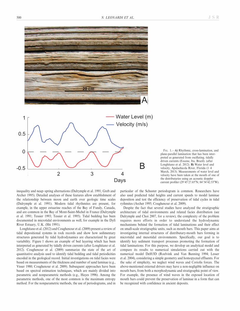
Longhitano et al. (2012) and Coughenour et al. (2009) present a review oftidal depositional systems in rock records and show how sedimentarystructures generated by tidal hydrodynamics are characterized by greatvariability. Figure 1 shows an example of bed layering which has beeninterpreted as generated by tidally driven currents (after Longhitano et al.2012). Coughenour et al. (2009) summarize the state of the art ofquantitative analysis used to identify tidal bedding and tidal periodicitiesencoded in the geological record. Initial investigations on tidal facies werebased on measurements of the thickness and number of sand laminae (e.g.,Visser 1980; Coughenour et al. 2009). Subsequent approaches have beenbased on spectral estimation techniques, which are mainly divided intoparametric and nonparametric methods (e.g., Hayes 1996). Among theparametric methods, one of the most common is the maximum entropymethod. For the nonparametric methods, the use of periodograms, and in

particular of the Schuster periodogram is common. Researchers havealso used predicted tidal heights and current speeds to model laminaedeposition and test the efficiency of preservation of tidal cycles in tidalrythmites (Archer 1995; Coughenour et al. 2009).

Despite the fact that several studies have analyzed the stratigraphicarchitecture of tidal environments and related facies distribution (seeDalrymple and Choi 2007, for a review), the complexity of the problemrequires more efforts in order to understand the hydrodynamicmechanisms behind the formation of tidal laminations and their effecton small-scale stratigraphic units, such as mouth bars. This paper aims atinvestigating internal structures of distributary-mouth bars forming inmicrotidal and mesotidal environments. Specifically, our goal is toidentify key sediment transport processes promoting the formation oftidal laminations. For this purpose, we develop an analytical model andcompare its results to numerical simulations carried out with thenumerical model Delft3D (Roelvink and Van Banning 1994; Lesseret al. 2004), considering a simple geometry and homopycnal effluents. Forthe sake of simplicity, we neglect wind waves and Coriolis forces. Theabove-mentioned external drivers may have a non-negligible influence onmouth bars, from both a morphodynamic and stratigraphic point of view.For example, the presence of wind waves in the exposed location ofmouth bars could prevent the preservation of laminae in a form that canbe recognized with confidence in ancient deposits.

FIG. 1.—A) Rhythmic, cross-lamination, andplane-parallel lamination that has been inter-preted as generated from oscillating, tidallydriven currents (Eocene, Itu, Brazil). (afterLonghitano et al. 2012). B) Water level andvelocity, Apalachicola River, Florida (1–4March, 2013). Measurements of water level andvelocity have been taken at the mouth of one ofthe distributaries using an acoustic dopplercurrent profiler (29u45927.650N; 84u54942.530W).

500 N. LEONARDI ET AL. J S R

The manuscript is organized as follows: Section 2 outlines thenumerical model features and its setup. Section 3 provides a theoreticalframework for the turbulent-jet theory at the channel mouth. Section 4describes hydrodynamic processes leading to the formation of tidalbedding. Section 5 deals with the spatial and temporal evolution of tidallaminae and their relationship to mouth-bar evolution. Section 6describes the analytical model. Section 7 provides a comparison betweenanalytical and numerical models. Section 8 deals with laminae charac-teristics as obtained from the numerical model. A set of conclusions ispresented in section 9.

2. Setup of Numerical Model

Mouth-bar formation and stratigraphy are studied by means of thecomputational fluid dynamics package Delft3D (Roelvink and VanBanning 1994; Lesser et al. 2004). Delft3D allows the simulation ofhydrodynamic flow, sediment transport, and related bed evolution(Lesser et al. 2004).

The model solves the shallow-water equations in two (depth-averaged)dimensions. These equations are the horizontal momentum equations, thecontinuity equation, the sediment transport equation, and a turbulenceclosure model. The vertical momentum equation reduces to the hydrostatic-pressure assumption because vertical accelerations are considered smallwith respect to gravitational acceleration and are not taken into account(Lesser et al. 2004). The sediment-transport and morphology modulesaccount for bed-load and suspended-load transport of cohesive andnoncohesive sediments and for the exchange of sediment between bedand water column. Suspended load is evaluated using the sedimentadvection–diffusion equation, and bed-load transport is computed usingempirical transport formulae. The bed-load transport formulation used inthis work is the one proposed by Van Rijn (1993). The model also takes intoaccount the vertical diffusion of sediments due to turbulent mixing andsediment settling due to gravity. In case of noncohesive sediments, theexchange of sediments between the bed and the flow is computed byevaluating sources and sinks of sediments near the bottom. Sources are dueto upward diffusion of sediments, and sinks are caused by sedimentsdropping out from the flow due to their settling velocities (Van Rijn 1993).In case of cohesive sediments, the Partheniades–Krone formulations forerosion and deposition are used (Partheniades 1965). In their formulation,the critical shear stress for erosion is always greater than or equal to the onefor deposition; therefore, intermediate shear-stress conditions may exist forwhich neither erosion nor deposition occurs. This cohesive sedimentsparadigm is in contrast to common assumptions for noncohesive sediments,for which deposition and erosion always occur simultaneously (Sanford and

Halka 1993). However, the existence of a critical shear stress for depositionis controversial. Winterwerp (2007) recently reviewed the cohesive-sedimentparadigm by means of literature data and was able to reproduceexperiments carried out by Krone (1962) without considering the presenceof a critical shear stress for deposition. Thus, he concluded that the so-calledcritical shear stress for deposition does not exist: it is simply a threshold forresuspension. The latter consideration was also postulated by Krone in hisoriginal report (Krone 1962). These findings are in agreement withobservations of Sanford and Halka (1993) in the upper Chesapeake Bay,for which model results show poor agreement with field observations whenthe presence of a critical shear stress for deposition is taken into account.

Therefore, we choose to assume a gross sedimentation rate of cohesivesediments equal to their settling flux wmcm, where wm and cm are settlingvelocity and concentration of the cohesive sediment fraction (Winterwerp2007). A possible implication of this hypothesis is an increase in the areawhere mud deposition is allowed.

Sediment-transport and morphology modules in Delft3D allowaccounting for multiple sediment fractions. The transport of eachsediment class is separately calculated taking into account the availabilityof each fraction in the bed. The erodible bed (comprising the channel) isdivided into multiple layers, and for each time step the exposed layer (thetransport layer) is the only one providing sediments to the flow. At everytime step the layer thickness is updated. In each layer, sediments areassumed to be vertically mixed. In our simulations, sediment erosionduring one time step never exceeds the thickness of a layer. We used 75initial layers of 2 cm thickness.

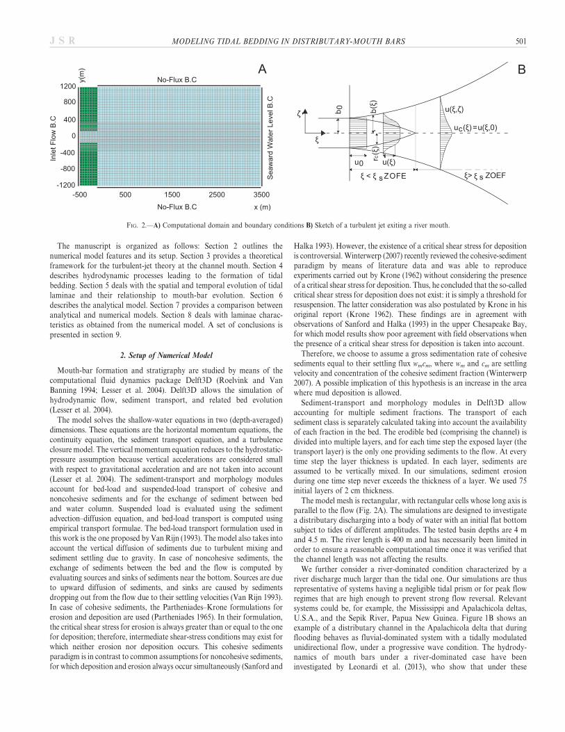
The model mesh is rectangular, with rectangular cells whose long axis isparallel to the flow (Fig. 2A). The simulations are designed to investigatea distributary discharging into a body of water with an initial flat bottomsubject to tides of different amplitudes. The tested basin depths are 4 mand 4.5 m. The river length is 400 m and has necessarily been limited inorder to ensure a reasonable computational time once it was verified thatthe channel length was not affecting the results.

We further consider a river-dominated condition characterized by ariver discharge much larger than the tidal one. Our simulations are thusrepresentative of systems having a negligible tidal prism or for peak flowregimes that are high enough to prevent strong flow reversal. Relevantsystems could be, for example, the Mississippi and Apalachicola deltas,U.S.A., and the Sepik River, Papua New Guinea. Figure 1B shows anexample of a distributary channel in the Apalachicola delta that duringflooding behaves as fluvial-dominated system with a tidally modulatedunidirectional flow, under a progressive wave condition. The hydrody-namics of mouth bars under a river-dominated case have beeninvestigated by Leonardi et al. (2013), who show that under these

FIG. 2.—A) Computational domain and boundary conditions B) Sketch of a turbulent jet exiting a river mouth.

MODELING TIDAL BEDDING IN DISTRIBUTARY-MOUTH BARS 501J S R

conditions a progressive wave at the river mouth is promoted by theestablishment of a drawdown profile at low tides and consequent flowacceleration (Leonardi et al. 2013).

The domain has three open boundaries: at the seaward boundary avarying water level is imposed to simulate sea-level variations due to tides.For the lateral boundaries, we impose a zero-flux boundary condition,consisting of imposing the gradient of the alongshore water level equal tozero (Fig. 2A). In the channel, a constant discharge is prescribed withvalues ranging from 900 m3/s to 2000 m3/s. Water level varies withsemidiurnal frequency (30 deg/h) and simulates tidal amplitudes rangingfrom 0.25 to 2.5 m. Initial conditions consist of a flat bottom and uniformbed composition with noncohesive sediments everywhere in the domain.Variable channel width-to-depth ratios have been used (90, 70, and 37) aswell as variable friction coefficients (Darcy-Weisbach friction coefficientsequal to 0.09, 0.02, and 0.04). Width-to-depth ratios were chosenconsidering that at the channel mouth the width is generally much largerthan depths and that width-to-depth ratios greater than 50 are common(Edmonds and Slingerland 2007). We prescribe a constant sediment inputof cohesive and noncohesive sediments for each numerical test. Thenoncohesive fraction has specific density of 2650 kg/m3, dry-bed density of1600 kg/m3, and median sediment diameter D50 of 200 mm. Characteristicsof cohesive sediments were chosen in agreement with values provided byBerlamont (1993). Specific density is 2650 kg/m3, dry-bed density is 500kg/m3, and settling velocities vary from 0.0001 m/s to 0.001 m/s.

3. Theoretical Framework for the Turbulent Jet at a River Mouth

As distributary channels discharge into a body of water, they behavelike a turbulent jet, experiencing mixing and diffusion (e.g., Bates 1953;Canestrelli et al. 2007, 2010; Wright and Coleman 1974; Ozsoy andUnluata 1982; Wright 1977; Rowland et al. 2009; Rowland et al. 2010;Falcini and Jerolmack 2010; Nardin and Fagherazzi 2012; Nardin et al.2013; Leonardi et al. 2013).

In coastal areas vertical motions are negligible respect to horizontal onesand the shallow water approximation is widely accepted (e.g., Ozsoy andUnluata 1982). Under these conditions the integral-jet theory is generallyapplicable and the turbulent jet has a symmetrical geometric structure withrespect to the longitudinal axis (Abramovich 1963). The jet can be dividedinto two regions: a zone of flow establishment (ZOFE) and a zone ofestablished flow (ZOEF). The first zone is characterized by a core ofconstant velocity, while the second one is characterized by an exponentiallydecreasing centerline velocity and a self-similar profile for the transversevelocity. The transition between the two zones is the downstream locationat which turbulence generated at the margins of the jet propagates towardsthe center (Bates 1953; Abramovich 1963).

Ozsoy (1977, 1986) proposed an analytical solution for jet parametersand sediment transport in the nearshore area in the vicinity of tidal inlets.The advection–diffusion equation is used to guarantee the conservation ofmass of sediments discharged by the river and experiencing gravitationalsettling. In this framework an ambient concentration distribution can betaken into account, and it is assumed that sediment concentration is smallwith respect to fluid density, with small density variations not contributingto the momentum balance. To compute centerline velocity, jet half-width,and centerline sediment concentrations in case of flat bottom with friction,the following normalized parameters are defined (Fig. 2B):

j~x

b0, f~

y

b jð Þ , H jð Þ~ h

h0, B jð Þ~ b jð Þ

b0, U jð Þ~ uc

u0,

js~xs

b0, R jð Þ~ rc

r0, C jð Þ~ cc

c0,

CA jð Þ~ ca

c0, c~

b0w

h0u0, y~

u0

ucr

, m~fb0

h0

ð1Þ

where b0 is the inlet half-width, b (j) is the jet half-width, h0 is the inletdepth, h is the water depth, r0 is the jet core at the inlet, rc is the jet core, u0 isthe centerline jet velocity at the inlet, uc is the centerline velocity, c0 is theconcentration at the inlet, ca is the ambient concentration, cc is thecenterline concentration, f is the Darcy and Weisbach friction coefficient, wis the sediment settling velocity, ucr is the critical shear velocity and xs is theend coordinate for the core region and marks the passage between ZOFEand ZOEF. xs is found imposing the normalized jet core half-width R equalto zero in the ZOFE equations (Ozsoy and Unluata 1982, 1986) (Fig. 2B,Equation 2). The depth-averaged equation of momentum and theadvection–diffusion equation are then solved, using the quasi-steadinessand self-similarity assumptions. The solution along the centerline in case offlat bottom with friction is, for the ZOFE (j , js):

U jð Þ~1,

R jð Þ~ I1e{mj{I2 1zajð ÞI1{I2

B jð Þ~ 1{I2ð Þ 1zajð Þ{ 1{I1ð Þe{mj

I1{I2

C jð Þ~ X{ I1{I4ð ÞH B{Rð ÞCA

RzI4 B{Rð Þ½ �H

ð2Þ

and for the ZOEF (j . js):

U jð Þ~ e{mj

ðe{2mjs z2aI2

mI1e{mjs {e{mj� �

Þ1=2

B jð Þ~ emj

I2ðe{2mjs z

2aI2

mI1e{mjs {e{mj� �

Þ

C jð Þ~ X{ I1{I4ð ÞHUBCA

RzI4B½ �HU

ð3Þ

where U(j) is the nondimensional centerline velocity, B(j) is thenondimensional jet half-width, C(j) is the nondimensional centerlineconcentration, R(j) is the nondimensional jet-core half-width, a 5 0.036in the ZOFE, a 5 0.05 in the ZOEF and I1, I2, and I4 are numericalconstants equal to 0.450, 0.316, and 0.368 respectively.

The quantities X and M are

X jð Þ~ 1P

Ð j

0PMdjz1

n oM jð Þ~aHUCAzc y2U2 I2{I5ð Þ{ 1{I3ð Þ

� �B{Rð ÞCA

z I1{I4ð ÞHU B{Rð ÞCAQ

ð4Þ

with

P jð Þ~exp

ðj

0

Q dj ð5Þ

Q jð Þ~ c RzI3 B{Rð Þ½ �{cy2U2 RzI5 B{Rð Þ½ �HU RzI4 B{Rð Þ½ � ð6Þ

where I3 and I5 are numerical constants equal to 0.6 and 0.278 respectively.Note that for CA (nondimensional ambient concentration) equal to

zero, M(j) goes to zero as well. These equations are used in Section 5 asthe starting point for the process-based model.

The variables X(j), M(j), P(j), and Q jð Þ can be used to write, in amore convenient form, the normalized equation for sediment concentra-tion distribution integrated across the jet cross section:

dX jð Þdj

zQ jð ÞX jð Þ~M jð Þ ð7Þ

4. Formation of Inter-Layered Bedding

Herein we introduce conceptual considerations on processes allowingthe formation of tidal bedding. Three main factors regulate the formation

502 N. LEONARDI ET AL. J S R

of tidal laminae: i) availability of at least two sediment fractions isnecessary to guarantee the presence of multiple facies. ii) Alternatingdeposition of these two sediment fractions is also required. In case of onesediment fraction continuously being deposited across the entire area,intermittent deposition of a second fraction is sufficient to guarantee theestablishment of laminae. iii) Sediment and settling characteristics such assediment concentration, settling velocity, bottom friction, and tidalamplitude may play an important role in defining bedding features.

The alternation of erosion and deposition is dictated mainly byvariations in shear velocity at the bottom. Tides, as well as varyingdischarge conditions, are responsible for such variability of bottom shearvelocity. In the presence of sand and mud, as in our numerical tests,variability throughout the tidal cycle of areas allowing mud deposition,triggered by variations in shear velocity, is expected to be greater thancorresponding variability in sand deposits. This is mainly due to highvalues of settling velocity and critical shear stress for erosion of sand withrespect to mud. Under these conditions small variations in shear velocityslightly affect the erosion of sand, and sand deposition continues to occurmainly near the river mouth.

From numerical-model results it is possible to evaluate net depositionas the difference between gross deposition (D) and erosion (E) fordifferent instants of the tidal cycle, as a function of different river-mouthvelocities and water depths.

Two possible cases lead to zero net deposition: for E ? 0, netdeposition is zero when E 5 D. For E 5 0, net deposition is zero whenD 5 0. These two behaviors can be observed for different sedimentfractions: for fine sediment fractions, the shear stress is expected to exceedits critical value near the river mouth (this condition also covers E . Dcases) and the condition E 5 D determines locations of points of zeronet deposition. For coarse sediment fractions, the shear stress does notexceed its critical value and deposition occurs around the river mouth in atidal cycle. Erosion is not expected to occur in the rest of the domain dueto lower shear stress far from the river mouth. Thus, in the latter case thereduction in sediment concentration in the water column of sand-sizematerial is the only process leading to zero net deposition.

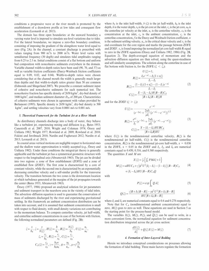
Mud net deposition is shown in Figure 3B for a tidal range equal to0.75 m (Fig. 3A) and for three instants of the tidal cycle (Fig. 3B). Forthis fine sediment fraction, a region of alternating negative and positivenet deposition is present due to variations in shear velocity at differentinstants of the tidal cycle. Here, xmin and xmiax are the minimum andmaximum longitudinal coordinates where net deposition reaches a zerovalue within a tidal cycle. The region between xmin , x , xmax is apotential lamination area, assuming the deposition of a second fraction ofsediments (e.g., sand) everywhere in this zone.

In Figure 3C, yellow bars indicate simultaneous deposition of bothmud and sand, and green bars indicate mud erosion and only sanddeposition at that specific tidal instant. The result is a lamination extentgoing from xmin to xmin and an area characterized by continuousdeposition of both sediment fractions beyond xmax that extends up to thelimit of sand deposit (sand limit, Fig. 3C).

The lamination extent may be substantially reduced if sand depositiondoes not reach xmax. The sand and mud mixture zone and the mud-onlyzones are limited by sediment availability as well.

5. Spatial and Temporal Patterns of Tidal Laminae

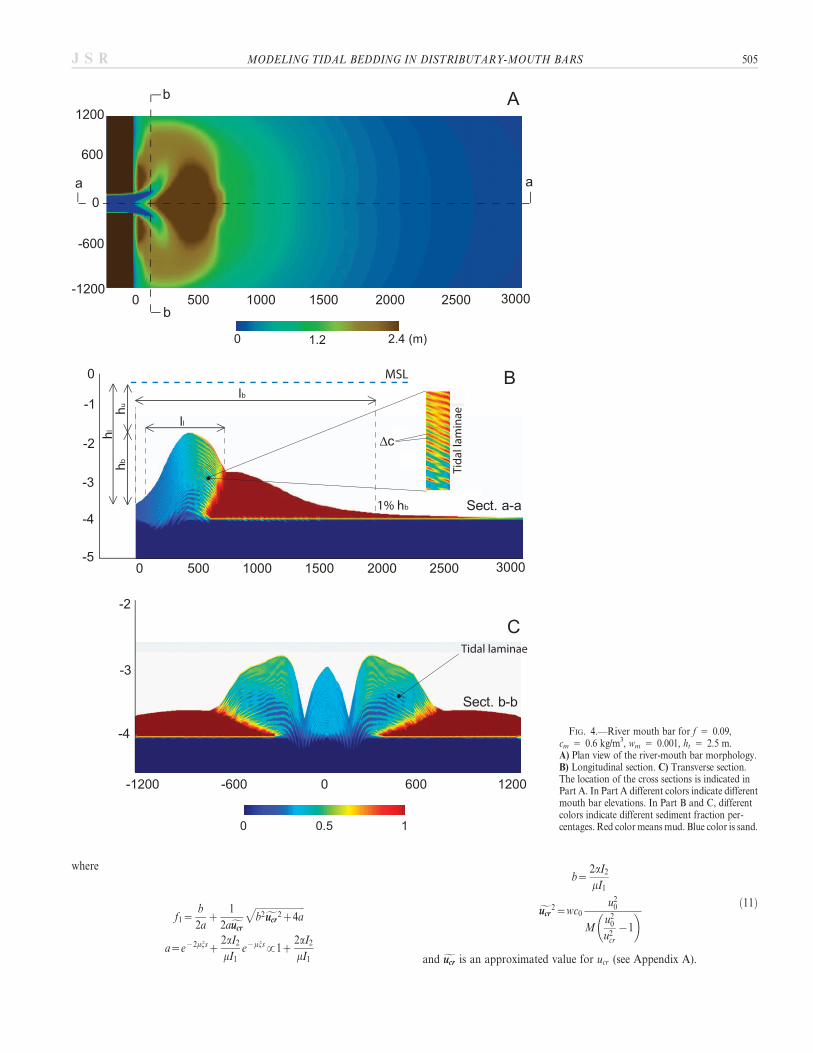
The model Delft3D is able to simulate the formation of mouth bars andthe presence of tidal laminations in the deposits. Figure 4A shows a planarview of the morphology of a simulated mouth bar. Figures 4B and C showtwo cross sections of the mouth bar. Different colors represent differentpercentages of sediment fractions. Red means mud in the absence of sand,and blue means sand and no mud. It is possible to notice that tidallaminations are clearly present only on the distal side of the mouth bar and

appear to end rapidly into the muddy prodelta deposits. The extent of tidallaminae increases during mouth-bar shoaling (i.e., the extent grows withelevation). Figure 4 also indicates variables useful to describe mouth-bargeometry such as mouth-bar length (lb) and height (hb).

Following a notation similar to that of Edmonds and Slingerland (2007),hu and hl are defined as the water depth above the peak of the mouth barand the river depth at the landward boundary (water depths being referredto mean sea level). According to the authors the formation of mouth barsgoes through different phases. The first phase is the initial deposition due toa decrease in jet momentum and consequent sediment settling. The secondphase is connected to flow acceleration at the top of the bar and consequentbar progradation. Finally, the bar stops prograding and starts widening,once it is high enough to force fluid around it. The latter step starts for hu/hl

values around 0.6 (Edmonds and Slingerland 2007).

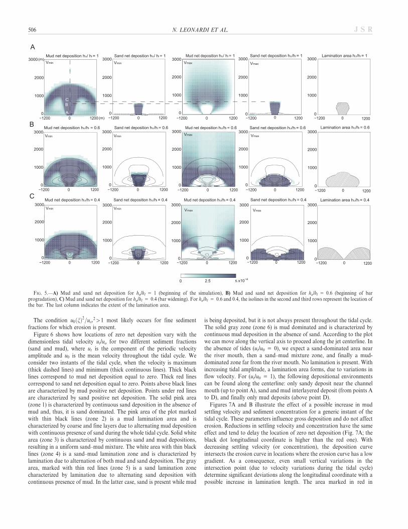
Mud net deposition and sand net deposition have been evaluated atdifferent instants of the tidal cycle, when velocity is at its maximum andminimum, and for different stages of the mouth bar evolution. Wecalculated net deposition for hu/hl equal to 1, 0.6, and 0.4. Figure 5A, B,and C refer to these ratios, showing net deposition for mud and sand, fora tidal amplitude ht equal to 2.5 m and for the minimum and maximumvelocity during the tidal cycle. Figure 5A represents net depositionalpatterns at the earliest stage of the simulation, when the mouth bar is notyet formed. Net depositional patterns maintain the same trends for smallmouth-bar elevations. Lamination is going to occur in the area betweenpoints A and B due to alternated presence of mud. In the area betweenpoints B and C, we are going to have lamination as well, this time due toalternating sand deposition, in the presence of mud.

For hu/hl ratios of 0.6 (Fig. 5B), the bar is at its prograding stage. Thelamination area is extensive and comprises the whole footprint of the barwhere fluid flow is accelerated. For low flow velocities, both mud andsand are able to settle on the top of the bar. However, for high velocitiesonly sand can be deposited because of its higher settling velocity, whilemud is eroded. Around the centerline, where sand is deposited during theentire tidal cycle, sand and mud layers are produced by intermittent muddeposition. At the two sides of the river mouth, either sand or muddeposits are present due to the absence of the other grain size. The finalresult is an expansion in time of the lamination area both longitudinallyand transversally (Fig. 4).

For hu/hl ratios of 0.4 (Fig. 5C), channelization around the bar begins.During periods of low velocity, depositional patterns are similar to thatobserved for previous hu/hl ratios. However, during periods of highvelocity and low water level, depositional patterns change because theflow is confined at the two sides of the bar. The result is that lamination infront of the bar ceases, while lamination at the two sides increases.

6. Analytical Model for Facies Distribution

According to considerations presented in Section 3, laminae extent dueto alternate erosion and deposition of only one sediment fraction isconfined between two points, xmin and xmin where net deposition is equalto zero when the tidal flow is minimum and maximum.

Given the analytical formulations for centerline velocity and concen-tration presented in Section 2, it is possible to evaluate the centerlinelongitudinal coordinates at which net deposition is equal to zero at everyinstant of the tidal cycle and for each sediment fraction. Gross deposition,D, and erosion, E, along the centerline are evaluated as

D~wc jð Þ ð8Þ

E~dMu jð Þ2

ucr2

{1

!ð9Þ

where d 5 0 foru jð Þ2

ucr2

ƒ1, and d 5 1 foru jð Þ2

ucr2

w1.

MODELING TIDAL BEDDING IN DISTRIBUTARY-MOUTH BARS 503J S R

For cohesive sediment fractions, M is the erosion parameter of thePartheniades–Krone formulation. For noncohesive sediment fractions, M

is obtained from the pick-up function proposed by Van Rijn (1993).

For a sediment fraction such that u0 jð Þ2=ucr2ƒ1, erosion is prevented

at the river mouth, and, because the velocity decreases with distance fromthe mouth, no erosion is expected to occur in the whole domain.Therefore, zero net deposition occurs only when sediment settling isnegligible, i.e., the concentration C jð Þ in the water column is zero

(Equation 3). For a sediment fraction such that u0 jð Þ2=ucr2w1, the

resulting nondimensional coordinate, j, at which net deposition is zero ata certain instant is obtained by imposing U(j) (Equation 3) equal toUcr(j) and by solving the second-degree equation in emj:

ejj~log f1ð Þ

mð10Þ

FIG. 3.—A) Water-level variations and tidallyinduced velocity variations in 18 hours. B) Mudnet deposition along the mouth-bar centerline atthree instants within a tidal cycle (Tmin, T0, andTmax). Time instants are indicated in Part A. Thecontinuous black line represents net depositionof mud during periods of low velocity (instantTmin), and the dashed line represents net depo-sition for high velocity (instant Tmax). The dottedline is the net deposition for intermediatevelocity (instant T0). xmin is the longitudinalcoordinate of zero net deposition at low velocity.xmax is the longitudinal coordinate of zero netdeposition at high velocity. C) Green barsrepresent mud negative net deposition and sandpositive net deposition at that specific tidalinstant. Yellow bars indicate simultaneous de-position of mud and sand. Red bars indicateareas where there is deposition of only mud. Thesand limit is the location beyond which sanddeposition ceases. Plus and minus signs indicatepositive and negative mud deposition.

504 N. LEONARDI ET AL. J S R

where

f1~b

2az

1

2afucrucr

ffiffiffiffiffiffiffiffiffiffiffiffiffiffiffiffiffiffiffiffiffiffib2fucrucr

2z4ap

a~e{2mjsz2aI2

mI1e{mjs!1z

2aI2

mI1

b~2aI2

mI1

fucrucr2~wc0

u20

Mu2

0

u2cr

{1

� � ð11Þ

and fucrucr is an approximated value for ucr (see Appendix A).

FIG. 4.—River mouth bar for f 5 0.09,cm 5 0.6 kg/m3, wm 5 0.001, ht 5 2.5 m.A) Plan view of the river-mouth bar morphology.B) Longitudinal section. C) Transverse section.The location of the cross sections is indicated inPart A. In Part A different colors indicate differentmouth bar elevations. In Part B and C, differentcolors indicate different sediment fraction per-centages. Red color means mud. Blue color is sand.

MODELING TIDAL BEDDING IN DISTRIBUTARY-MOUTH BARS 505J S R

The condition u0 jð Þ2=ucr2w1 most likely occurs for fine sediment

fractions for which erosion is present.

Figure 6 shows how locations of zero net deposition vary with thedimensionless tidal velocity ut/uo for two different sediment fractions(sand and mud), where ut is the component of the periodic velocityamplitude and u0 is the mean velocity throughout the tidal cycle. Weconsider two instants of the tidal cycle, when the velocity is maximum(thick dashed lines) and minimum (thick continuous lines). Thick blacklines correspond to mud net deposition equal to zero. Thick red linescorrespond to sand net deposition equal to zero. Points above black linesare characterized by mud positive net deposition. Points under red linesare characterized by sand positive net deposition. The solid pink area(zone 1) is characterized by continuous sand deposition in the absence ofmud and, thus, it is sand dominated. The pink area of the plot markedwith thin black lines (zone 2) is a mud lamination area and ischaracterized by coarse and fine layers due to alternating mud depositionwith continuous presence of sand during the whole tidal cycle. Solid whitearea (zone 3) is characterized by continuous sand and mud depositions,resulting in a uniform sand–mud mixture. The white area with thin blacklines (zone 4) is a sand–mud lamination zone and is characterized bylamination due to alternation of both mud and sand deposition. The grayarea, marked with thin red lines (zone 5) is a sand lamination zonecharacterized by lamination due to alternating sand deposition withcontinuous presence of mud. In the latter case, sand is present while mud

is being deposited, but it is not always present throughout the tidal cycle.The solid gray zone (zone 6) is mud dominated and is characterized bycontinuous mud deposition in the absence of sand. According to the plotwe can move along the vertical axis to proceed along the jet centerline. Inthe absence of tides (ut/u0 5 0), we expect a sand-dominated area nearthe river mouth, then a sand–mud mixture zone, and finally a mud-dominated zone far from the river mouth. No lamination is present. Withincreasing tidal amplitude, a lamination area forms, due to variations inflow velocity. For (ut/u0 5 1), the following depositional environmentscan be found along the centerline: only sandy deposit near the channelmouth (up to point A), sand and mud interlayered deposit (from points Ato D), and finally only mud deposits (above point D).

Figures 7A and B illustrate the effect of a possible increase in mudsettling velocity and sediment concentration for a generic instant of thetidal cycle. These parameters influence gross deposition and do not affecterosion. Reductions in settling velocity and concentration have the sameeffect and tend to delay the location of zero net deposition (Fig. 7A; theblack dot longitudinal coordinate is higher than the red one). Withdecreasing settling velocity (or concentration), the deposition curveintersects the erosion curve in locations where the erosion curve has a lowgradient. As a consequence, even small vertical variations in theintersection point (due to velocity variations during the tidal cycle)determine significant deviations along the longitudinal coordinate with apossible increase in lamination length. The area marked in red in

FIG. 5.—A) Mud and sand net deposition for hu/hl 5 1 (beginning of the simulation), B) Mud and sand net deposition for hu/hl 5 0.6 (beginning of barprogradation), C) Mud and sand net deposition for hu/hl 5 0.4 (bar widening). For hu/hl 5 0.6 and 0.4, the isolines in the second and third rows represent the location ofthe bar. The last column indicates the extent of the lamination area.

506 N. LEONARDI ET AL. J S R

Figure 7A represents positive net deposition for high settling velocity (orconcentration), and it is larger than the black marked area, representativeof positive net deposition for low values of these quantities. Therefore, forhigh values of mud settling velocity and concentration, it is reasonable toexpect a small lamination area near the river mouth and high mudcontent in the layers.

Figure 7B illustrates variations in lamination extent (zero netdeposition for mud in Fig. 6) due to a decreasing mud settling velocity.This is a direct consequence of variations in the intersection points ofFigure 7A. The laminae extension increases basinward for low settlingvelocities of the mud, while an increase in settling velocity (or sedimentconcentration) tends to increase landward deposition.

7. Comparison between Analytical and Numerical Model

The analytical model proposed in Section 6 does not take into accountbottom evolution and as a consequence the expansion of the laminationarea connected to the shoaling of the mouth bar (Fig. 4, Section 3).Figure 8 compares the length scale over which tidal laminae can formpredicted by the numerical model compared to that predicted by theanalytical model. Note that in our idealized models this length scalecorresponds to the length scale of the individual laminations themselves(as they are considered continuous). In a natural system, where there aremany additional processes at work, the length of individual laminationsmay be very different from the length of the zone under which they arestable (zones 2, 4, and 5 in Fig. 6).

As expected, the length of the lamination zone predicted by theanalytical model underestimates the results of the numerical model.However, there is a significant correlation between the two models withanalytical and numerical area of lamination having comparable trends(Fig. 8).

For the difference in mud content between successive layers, aqualitative comparison between the analytical and numerical modelscan be obtained by looking at its distribution along the centerline.

Figure 9 shows how Dc (blue line) and the maximum mud concentration(Cmax) (red line) vary along the centerline for a typical run with 2.5 mtidal amplitude. Given a certain longitudinal coordinate, Dc is theaverage, for multiple tidal cycles, of the difference in mud contentbetween two subsequent layers deposited at each tidal cycle.

Cmax is the maximum mud content, for all vertical layers. It is possibleto see that both curves are characterized by three main zones withdifferent slopes (A–B, B–C, and C–D). The three zones correspond to thethree different areas marked in Figure 6 (right y axis). Proceedingdownstream from the channel mouth along the centerline, we encounterlocations having increasing time of mud deposition (Fig. 3C). Mudcontent per layer (in layers where the percentage of mud is higher thanthat of sand) as well as maximum mud content can be reasonably relatedto the duration of time, throughout the tidal cycle, during which mud canbe deposited.

In the interval from A to B, mud deposition increases, but it isintermittent during the tidal cycle. All points are characterized byconstant deposition of sand. From B to C, mud deposition duration isstill increasing. The increased steepness is determined by the fact that, inthis area, sand is not always present, favoring a relative increase in mudcontent. In the interval from C to D mud deposition is constant and thepresence of sand is at its minimum, because the sand fraction is the onedetermining the formation of layers. In this case both mud concentrationand mud difference between different layers are at their maximum.Therefore maximum Dc occurs where lamination is determined by sandrather than by mud variability. From Figure 10 it is possible to note anincrease in mud content per layer with increasing longitudinal coordinate.A reduction in the laminae area for small tidal amplitudes is also evidentfrom Figure 10B.

8. Lamination Characteristics

By taking into account numerical and analytical model results, beddingcharacteristics along the centerline have been defined using the lamination

FIG. 6.—Facies model for river-mouth bars asobtained from Equations 2 to 13. On thelongitudinal axis, ut/u0 is the dimensionless tidalvelocity. On the vertical axis, j is the dimen-sionless longitudinal coordinate. Zone 1 ischaracterized by sand deposits in the absence ofmud. Zone 2 is a lamination area due toalternating mud deposition. Zone 3 is an areacharacterized by a homogeneous deposition ofmud and sand. Zone 4 is a sand–mud laminationarea. Zone 5 is characterized by alternating sanddeposition with constant presence of mud. Zone6 is mud dominated.

MODELING TIDAL BEDDING IN DISTRIBUTARY-MOUTH BARS 507J S R

length (ll), defined as the total length where tidal laminations can form,and the maximum difference in mud content (Dc) between two successivelayers (Fig. 4). The latter difference is the average of different Dc valuesalong the mouth-bar centerline (Fig. 4). Parameters Dc and ll werecalculated from our numerical tests for values of hu/hl equal to 0.4. Tounderstand how sediment characteristics and hydrodynamic conditionsaffect Dc and ll, we use dimensional analysis and Buckingam’s P theorem.Assuming constant values of erosion parameters and critical shearvelocity for the two sediment fractions, it follows that both the location ofzero net deposition j and the sediment concentration in the water column

C(j) (Equations 3, 9) at different instants of the tidal cycle depend on f,bo, ho, uo, w, co, and ht, where w and c0, are the settling velocity andconcentration at the river mouth of a certain sediment fraction.Considering the above independent variables for both mud and sand,and applying the P theorem, it is possible to obtain two functional

relationships forDc

cm

andll

b0

as a function of the following nondimensional

FIG. 7.—A) Erosion and deposition of mud along a mouth-bar centerline. Theblue line is the erosion curve. Red and black lines are gross deposition curves fordifferent values of settling velocity, wm, or sediment concentration, cm, of the mudat the river mouth. The red line corresponds to high values of w or c0. The red andblack dots are points of zero net deposition. Their position varies throughout thetidal cycle. The black point is characterized by a low gradient of the erosion curve.A vertical shift of the erosion curve during a tidal cycle causes larger variations inthe longitudinal coordinate of the black dot with respect to the red one. Incontrast, steeper gradients of the upper part of the erosion curve cause highdifferences between the marked areas at different instant of the tidal cycle. B) Linesof zero net deposition for the mud as in Figure 6 for different settling velocities.

FIG. 8.—Comparison between lamination lengths measured from numericalmodel results and calculated from the analytical model.

FIG. 9.—Percentage difference in mud content between successive layers along amouth-bar centerline (blue line) and maximum mud content (red line). Points A, B,C, and D are reported in Figure 6 as well.

508 N. LEONARDI ET AL. J S R

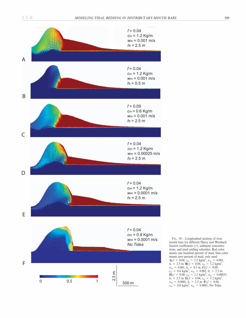
FIG. 10.—Longitudinal sections of rivermouth bars for different Darcy and Weisbachfriction coefficients ( f ), sediment concentra-tions, and mud settling velocities. Red colormeans one hundred percent of mud, blue colormeans zero percent of mud, only sand.A) f 5 0.04, cm 5 1.2 kg/m3, wm 5 0.001,ht 5 2.5 m. B) f 5 0.04, cm 5 1.2 kg/m3,wm 5 0.001, ht 5 0.5 m. C) f 5 0.09,cm 5 0.6 kg/m3, wm 5 0.001, ht 5 2.5 m.D) f 5 0.04, cm 5 1.2 kg/m3, wm 5 0.00025,ht 5 2.5 m. E) f 5 0.04, cm 5 1.2 kg/m3,wm 5 0.0001, ht 5 2.5 m. F) f 5 0.04,cm 5 0.8 kg/m3, wm 5 0.0001, No Tides.

MODELING TIDAL BEDDING IN DISTRIBUTARY-MOUTH BARS 509J S R

parameters: f ,b0

h0

,ht

h0

,cm

cs

,wm

ws

,wm

u0

, where u0 is the riverine velocity at mean

sea level, cm and cs are the mud and sand concentrations in the river, b0 isthe river-mouth half-width, h0 is the bottom depth for mean sea level andwm and ws are mud and sand settling velocity respectively. By assumingpower-law relationships and by means of a multiple regression analysiswe obtain the empirical expressions:

Dc

cm

~1:86f 0:3 b0

h0

0:2 ht

h0

0:4 cm

cs

0:01 wm

ws

0:24 wm

u0

0:27

ll

b0~0:79f {0:2 b0

h0

{0:2 ht

h0

0:2 cm

cs

{0:04 wm

ws

{0:01 wm

u0

{0:11ð12Þ

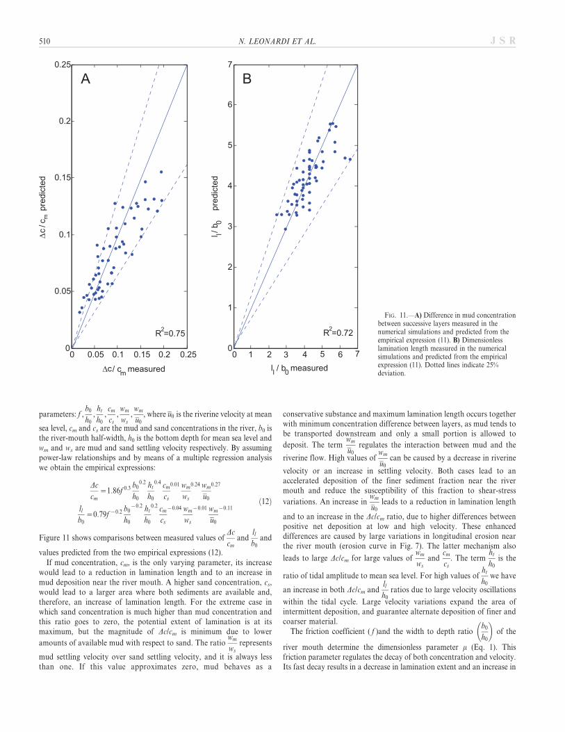
Figure 11 shows comparisons between measured values ofDc

cm

andll

b0and

values predicted from the two empirical expressions (12).

If mud concentration, cm, is the only varying parameter, its increasewould lead to a reduction in lamination length and to an increase inmud deposition near the river mouth. A higher sand concentration, cs,would lead to a larger area where both sediments are available and,therefore, an increase of lamination length. For the extreme case inwhich sand concentration is much higher than mud concentration andthis ratio goes to zero, the potential extent of lamination is at itsmaximum, but the magnitude of Dc/cm is minimum due to lower

amounts of available mud with respect to sand. The ratiowm

ws

represents

mud settling velocity over sand settling velocity, and it is always lessthan one. If this value approximates zero, mud behaves as a

conservative substance and maximum lamination length occurs togetherwith minimum concentration difference between layers, as mud tends tobe transported downstream and only a small portion is allowed to

deposit. The termwm

u0regulates the interaction between mud and the

riverine flow. High values ofwm

u0can be caused by a decrease in riverine

velocity or an increase in settling velocity. Both cases lead to anaccelerated deposition of the finer sediment fraction near the rivermouth and reduce the susceptibility of this fraction to shear-stress

variations. An increase inwm

u0leads to a reduction in lamination length

and to an increase in the Dc/cm ratio, due to higher differences betweenpositive net deposition at low and high velocity. These enhanceddifferences are caused by large variations in longitudinal erosion nearthe river mouth (erosion curve in Fig. 7). The latter mechanism also

leads to large Dc/cm for large values ofwm

ws

andcm

cs

. The termht

h0is the

ratio of tidal amplitude to mean sea level. For high values ofht

h0

we have

an increase in both Dc/cm andll

h0ratios due to large velocity oscillations

within the tidal cycle. Large velocity variations expand the area ofintermittent deposition, and guarantee alternate deposition of finer andcoarser material.

The friction coefficient ( f )and the width to depth ratiob0

h0

� �of the

river mouth determine the dimensionless parameter m (Eq. 1). Thisfriction parameter regulates the decay of both concentration and velocity.Its fast decay results in a decrease in lamination extent and an increase in

FIG. 11.—A) Difference in mud concentrationbetween successive layers measured in thenumerical simulations and predicted from theempirical expression (11). B) Dimensionlesslamination length measured in the numericalsimulations and predicted from the empiricalexpression (11). Dotted lines indicate 25%deviation.

510 N. LEONARDI ET AL. J S R

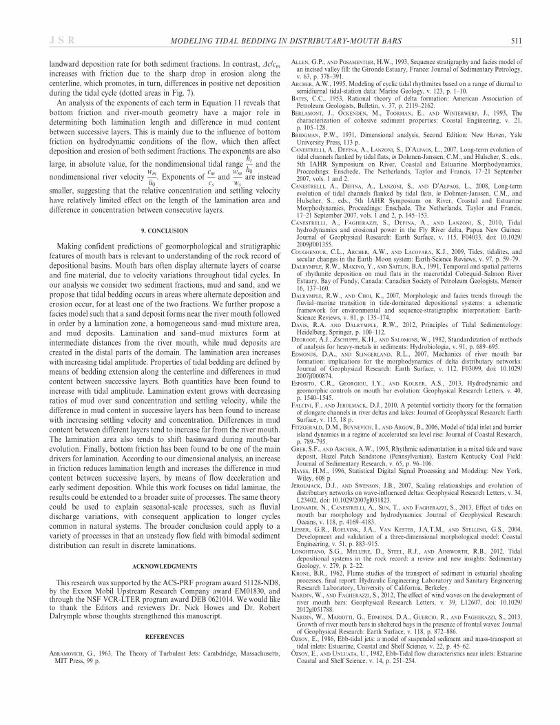
landward deposition rate for both sediment fractions. In contrast, Dc/cm

increases with friction due to the sharp drop in erosion along thecenterline, which promotes, in turn, differences in positive net depositionduring the tidal cycle (dotted areas in Fig. 7).

An analysis of the exponents of each term in Equation 11 reveals thatbottom friction and river-mouth geometry have a major role indetermining both lamination length and difference in mud contentbetween successive layers. This is mainly due to the influence of bottomfriction on hydrodynamic conditions of the flow, which then affectdeposition and erosion of both sediment fractions. The exponents are also

large, in absolute value, for the nondimensional tidal rangeht

h0and the

nondimensional river velocitywm

u0

. Exponents ofcm

cs

andwm

ws

are instead

smaller, suggesting that the relative concentration and settling velocityhave relatively limited effect on the length of the lamination area anddifference in concentration between consecutive layers.

9. CONCLUSION

Making confident predictions of geomorphological and stratigraphicfeatures of mouth bars is relevant to understanding of the rock record ofdepositional basins. Mouth bars often display alternate layers of coarseand fine material, due to velocity variations throughout tidal cycles. Inour analysis we consider two sediment fractions, mud and sand, and wepropose that tidal bedding occurs in areas where alternate deposition anderosion occur, for at least one of the two fractions. We further propose afacies model such that a sand deposit forms near the river mouth followedin order by a lamination zone, a homogeneous sand–mud mixture area,and mud deposits. Lamination and sand–mud mixtures form atintermediate distances from the river mouth, while mud deposits arecreated in the distal parts of the domain. The lamination area increaseswith increasing tidal amplitude. Properties of tidal bedding are defined bymeans of bedding extension along the centerline and differences in mudcontent between successive layers. Both quantities have been found toincrease with tidal amplitude. Lamination extent grows with decreasingratios of mud over sand concentration and settling velocity, while thedifference in mud content in successive layers has been found to increasewith increasing settling velocity and concentration. Differences in mudcontent between different layers tend to increase far from the river mouth.The lamination area also tends to shift basinward during mouth-barevolution. Finally, bottom friction has been found to be one of the maindrivers for lamination. According to our dimensional analysis, an increasein friction reduces lamination length and increases the difference in mudcontent between successive layers, by means of flow deceleration andearly sediment deposition. While this work focuses on tidal laminae, theresults could be extended to a broader suite of processes. The same theorycould be used to explain seasonal-scale processes, such as fluvialdischarge variations, with consequent application to longer cyclescommon in natural systems. The broader conclusion could apply to avariety of processes in that an unsteady flow field with bimodal sedimentdistribution can result in discrete laminations.

ACKNOWLEDGMENTS

This research was supported by the ACS-PRF program award 51128-ND8,by the Exxon Mobil Upstream Research Company award EM01830, andthrough the NSF VCR-LTER program award DEB 0621014. We would liketo thank the Editors and reviewers Dr. Nick Howes and Dr. RobertDalrymple whose thoughts strengthened this manuscript.

REFERENCES

ABRAMOVICH, G., 1963, The Theory of Turbulent Jets: Cambdridge, Massachusetts,MIT Press, 99 p.

ALLEN, G.P., AND POSAMENTIER, H.W., 1993, Sequence stratigraphy and facies model ofan incised valley fill: the Gironde Estuary, France: Journal of Sedimentary Petrology,v. 63, p. 378–391.

ARCHER, A.W., 1995, Modeling of cyclic tidal rhythmites based on a range of diurnal tosemidiurnal tidal-station data: Marine Geology, v. 123, p. 1–10.

BATES, C.C., 1953, Rational theory of delta formation: American Association ofPetroleum Geologists, Bulletin, v. 37, p. 2119–2162.

BERLAMONT, J., OCKENDEN, M., TOORMAN, E., AND WINTERWERP, J., 1993, Thecharacterization of cohesive sediment properties: Coastal Engineering, v. 21,p. 105–128.

BRIDGMAN, P.W., 1931, Dimensional analysis, Second Edition: New Haven, YaleUniversity Press, 113 p.

CANESTRELLI, A., DEFINA, A., LANZONI, S., D’ALPAOS, L., 2007, Long-term evolution oftidal channels flanked by tidal flats, in Dohmen-Janssen, C.M., and Hulscher, S., eds.,5th IAHR Symposium on River, Coastal and Estuarine Morphodynamics,Proceedings: Enschede, The Netherlands, Taylor and Francis, 17–21 September2007, vols. 1 and 2.

CANESTRELLI, A., DEFINA, A., LANZONI, S., AND D’ALPAOS, L., 2008, Long-termevolution of tidal channels flanked by tidal flats, in Dohmen-Janssen, C.M., andHulscher, S., eds., 5th IAHR Symposium on River, Coastal and EstuarineMorphodynamics, Proceedings: Enschede, The Netherlands, Taylor and Francis,17–21 September 2007, vols. 1 and 2, p. 145–153.

CANESTRELLI, A., FAGHERAZZI, S., DEFINA, A., AND LANZONI, S., 2010, Tidalhydrodynamics and erosional power in the Fly River delta, Papua New Guinea:Journal of Geophysical Research: Earth Surface, v. 115, F04033, doi: 10.1029/2009jf001355.

COUGHENOUR, C.L., ARCHER, A.W., AND LACOVARA, K.J., 2009, Tides, tidalites, andsecular changes in the Earth–Moon system: Earth-Science Reviews, v. 97, p. 59–79.

DALRYMPLE, R.W., MAKINO, Y., AND SAITLIN, B.A., 1991, Temporal and spatial patternsof rhythmite deposition on mud flats in the macrotidal Cobequid–Salmon RiverEstuary, Bay of Fundy, Canada: Canadian Society of Petroleum Geologists, Memoir16, 137–160.

DALRYMPLE, R.W., AND CHOI, K., 2007, Morphologic and facies trends through thefluvial–marine transition in tide-dominated depositional systems: a schematicframework for environmental and sequence-stratigraphic interpretation: Earth-Science Reviews, v. 81, p. 135–174.

DAVIS, R.A. AND DALRYMPLE, R.W., 2012, Principles of Tidal Sedimentology:Heidelberg, Springer, p. 100–112.

DEGROOT, A.J., ZSCHUPPE, K.H., AND SALOMONS, W., 1982, Standardization of methodsof analysis for heavy-metals in sediments: Hydrobiologia, v. 91, p. 689–695.

EDMONDS, D.A., AND SLINGERLAND, R.L., 2007, Mechanics of river mouth barformation: implications for the morphodynamics of delta distributary networks:Journal of Geophysical Research: Earth Surface, v. 112, F03099, doi: 10.1029/2007jf000874.

ESPOSITO, C.R., GEORGIOU, I.Y., AND KOLKER, A.S., 2013, Hydrodynamic andgeomorphic controls on mouth bar evolution: Geophysical Research Letters, v. 40,p. 1540–1545.

FALCINI, F., AND JEROLMACK, D.J., 2010, A potential vorticity theory for the formationof elongate channels in river deltas and lakes: Journal of Geophysical Research: EarthSurface, v. 115, 18 p.

FITZGERALD, D.M., BUYNEVICH, I., AND ARGOW, B., 2006, Model of tidal inlet and barrierisland dynamics in a regime of accelerated sea level rise: Journal of Coastal Research,p. 789–795.

GREB, S.F., AND ARCHER, A.W., 1995, Rhythmic sedimentation in a mixed tide and wavedeposit, Hazel Patch Sandstone (Pennsylvanian), Eastern Kentucky Coal Field:Journal of Sedimentary Research, v. 65, p. 96–106.

HAYES, H.M., 1996, Statistical Digital Signal Processing and Modeling: New York,Wiley, 608 p.

JEROLMACK, D.J., AND SWENSON, J.B., 2007, Scaling relationships and evolution ofdistributary networks on wave-influenced deltas: Geophysical Research Letters, v. 34,L23402, doi: 10.1029/2007gl031823.

LEONARDI, N., CANESTRELLI, A., SUN, T., AND FAGHERAZZI, S., 2013, Effect of tides onmouth bar morphology and hydrodynamics: Journal of Geophysical Research:Oceans, v. 118, p. 4169–4183.

LESSER, G.R., ROELVINK, J.A., VAN KESTER, J.A.T.M., AND STELLING, G.S., 2004,Development and validation of a three-dimensional morphological model: CoastalEngineering, v. 51, p. 883–915.

LONGHITANO, S.G., MELLERE, D., STEEL, R.J., AND AINSWORTH, R.B., 2012, Tidaldepositional systems in the rock record: a review and new insights: SedimentaryGeology, v. 279, p. 2–22.

KRONE, B.R., 1962, Flume studies of the transport of sediment in estuarial shoalingprocesses, final report: Hydraulic Engineering Laboratory and Sanitary EngineeringResearch Laboratory, University of California, Berkeley.

NARDIN, W., AND FAGHERAZZI, S., 2012, The effect of wind waves on the development ofriver mouth bars: Geophysical Research Letters, v. 39, L12607, doi: 10.1029/2012gl051788.

NARDIN, W., MARIOTTI, G., EDMONDS, D.A., GUERCIO, R., AND FAGHERAZZI, S., 2013,Growth of river mouth bars in sheltered bays in the presence of frontal waves: Journalof Geophysical Research: Earth Surface, v. 118, p. 872–886.

OZSOY, E., 1986, Ebb-tidal jets: a model of suspended sediment and mass-transport attidal inlets: Estuarine, Coastal and Shelf Science, v. 22, p. 45–62.

OZSOY, E., AND UNLUATA, U., 1982, Ebb-Tidal flow characteristics near inlets: EstuarineCoastal and Shelf Science, v. 14, p. 251–254.

MODELING TIDAL BEDDING IN DISTRIBUTARY-MOUTH BARS 511J S R

PARTHENIADES, E., 1965. Erosion and deposition of cohesive soils: American Society ofCivil Engineers, Journal of the Hydraulics Division, Proceedings, v. 92, p. 79–81.

ROELVINK, J.A., AND VAN BANNING, G.K.F.M., 1994. Design and development of Delft-3D and application to coastal morphodynamics, in Verwey, A., Minns, A.W.,Babovic, V., and Maksimovic, M., eds., Hydroinformatics ’94: Rotterdam, Balkema,p. 451–456.

ROWLAND, J.C., STACEY, M.T., AND DIETRICH, W.E., 2009, Turbulent characteristics of ashallow wall-bounded plane jet: experimental implications for river mouth hydrody-namics: Journal of Fluid Mechanics, v. 627, p. 423–449.

ROWLAND, J.C., DIETRICH, W.E., AND STACEY, M.T., 2010, Morphodynamics ofsubaqueous levee formation: insights into river mouth morphologies arising fromexperiments: Journal of Geophysical Research: Earth Surface, v. 115, #F04007.

SANFORD, L.P., AND HALKA, J.P., 1993, Assessing the paradigm of mutually exclusiveerosion and deposition of mud, with examples from Upper Chesapeake Bay: MarineGeology, v. 114, p. 37–57.

SCHATZINGER, R.A., AND TOMUTSA, L., 1999, Multiscale heterogeneity characterizationof tidal channel, tidal delta, and foreshore facies, Almond Formation outcrops, RockSprings uplift, Wyoming: Reservoir Characterization: Recent Advances, v. 71,p. 45–55.

SHI, Z., 1991, Tidal bedding and tidal cyclicities within the intertidal sediments of amicrotidal estuary, Dyfi River Estuary, West Wales, U.K.: Sedimentary Geology,v. 73, p. 43–58.

SYDOW, J., AND ROBERTS, H.H., 1994, Stratigraphic framework of a late Pleistoceneshelf-edge delta, northeast Gulf-of-Mexico: American Association of PetroleumGeologists, Bulletin, v. 78, p. 1276–1312.

TESSIER, B., 1993, upper intertidal rhythmites in the Mont-Saint-Michel Bay (NWFrance): perspectives for paleoreconstruction: Marine Geology, v. 110, p. 355–367.

TESSIER, B., ARCHER, A.W., LANIER, W.P., AND FELDMAN, H.R., 1995, Comparison ofancient tidal rhythmites (Carboniferous of Kansas and Indiana, USA) with modernanalogues (the Bay of Mont-Saint-Michel, France), in Flemming, B.W. andBartholoma, A., Tidal Signatures in Modern and Ancient Sediments: Oxford,Blackwell, p. 259–271.

VAN LEDDEN, M., WANG, Z.B., WINTERWERP, H., AND DE VRIEND, H., 2004, Sand–mudmorphodynamics in a short tidal basin: Ocean Dynamics, v. 54, p. 385–391.

VAN RIJN, L.C., 1993, Principles of Sediment Transport in Rivers, Estuaries and CoastalSeas: Amsterdam, Aqua Publications, 715 p.

VISSER, M.J., 1980, Neap–spring cycles reflected in Holocene subtidal large-scalebedform deposits: a preliminary note: Geology, v. 8, p. 543–546.

WHITE, C.D., WILLIS, B.J., DUTTON, S.P., BHATTACHARYA, J.P., AND NARAYANAN, K.,2004, Sedimentology, statistics, and flow behavior for a tide-influenced deltaicsandstone, Frontier Formation, Wyoming, United States, in Grammer, G.M., Harris,P.M., and Eberli, G.P., eds., Integration of Outcrop and Modern Analogs inReservoir Modeling: American Association of Petroleum Geologists, Memoir 80,p. 129–152.

WINTERWERP, J.C., 2007, On the sedimentation rate of cohesive sediment, in Maa,J.P.-Y., Sanford, L.P., and Schoellhamer, D.H., Coastal and Estuarine Fine SedimentProcesses: Proceedings in Marine Science, v. 8, p. 209–226.

WRIGHT, L.D., 1977, Sediment transport and deposition at river mouths: synthesis:Geological Society of America, Bulletin, v. 88, p. 857–868.

WRIGHT, L.D., AND COLEMAN, J.M., 1974, Mississippi River Mouth Processes: effluentdynamics and morphologic development: Journal of Geology, v. 82, p. 751–778.

Received 20 August 2013; accepted 14 March 2014.

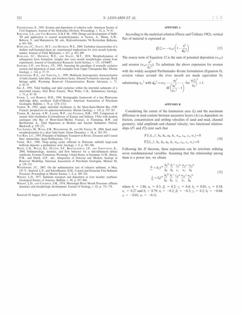
APPENDIX A

According to the analytical solution (Ozsoy and Unluata 1982), verticalflux of material is expressed as

Q jð Þ~{wmc 1{u2fucrucr

2

� �ð13Þ

The source term of Equation 12 is the sum of potential deposition (wmc)

and erosion (wmcu2

ucr2). To substitute the above expression for erosion

with the widely accepted Partheniades–Krone formulation (Equation 8),erosion values around the river mouth are made equivalent by

substituting ucr2 with fucrucr

2~wc0u0

2

Mu0

2

ucr2{1

� � foru jð Þ2

ucr2

w1.

APPENDIX B

Considering the extent of the lamination area (ll) and the maximumdifference in mud content between successive layers (Dc) as dependent onfriction, concentration and settling velocities of sand and mud, channelgeometry, tidal amplitude and channel velocity, two functional relation-ships (F1 and F2) exist such that

F1 Dc, f , b0, h0, u0, ht, wm, cm, cs, wsð Þ~0

F2 ll , f , b0, h0, u0, ht, wm, cm, cs, wsð Þ~0ð14Þ

Following the P theorem, these expressions can be rewritten utilizingseven nondimensional variables. Assuming that the relationship amongthem is a power law, we obtain

Dccm

~qCf acb0

h0

bc ht

h0

cc cm

cs

dc wm

ws

ec wm

u0

kc

llb0

~ql fal

b0

h0

bl ht

h0

cl cm

cs

dl wm

ws

el wm

u0

kl

ð15Þ

where hc 5 1.86; ac 5 0.3; bc 5 0.2; cc 5 0.4; dc 5 0.01; ec 5 0.24;kc 5 0.27 and hl 5 0.79; al 5 20.2; bl 5 20.2; cl 5 0.2; dl 5 20.04;el 5 20.01; kl 5 20.11.

512 N. LEONARDI ET AL. J S R