MODELING THE MAGNETO- RHEOLOGICAL …umpir.ump.edu.my/4426/1/cd6632_63.pdfviii table of contents title page title page examiner declaration i supervisor’s declaration ii

MODELING THE MAGNETO- RHEOLOGICAL DAMPER USING

RECURRENT NEURAL NETWORK METHOD

MUHAMMAD AFIQ NAQUIDDIN BIN ABD RAHMAN

This thesis is submitted as partial fulfillment of the requirements for the award of the

Bachelor of Mechanical Engineering

Faculty of Mechanical Engineering

University Malaysia Pahang

JUNE, 2012

vi

ABSTRACT

This thesis is study about modeling the Magnetorheological damper using

Recurrent Neural Network method. Five different values of current were used in order to

modeling the MR damper, which are 0.0 ampere, 0.5 ampere, 1.0 ampere, 1.5 ampere and

2.0 ampere. In order to modeling the MR damper, the graph of simulation damper will be

compared with the experimental damper. The results will get the Square Error for the

simulation damper. Then, the Root Mean Square Error will be calculated to get the

difference between the simulation damper and experimental damper. The results show

that the lowest RMSE for the simulation damper were value 0.4008, while the highest

RMSE is 1.9882. From the results also, the better current value to modeling the MR

damper is using the MR damper with the lowest RMSE.

vii

ABSTRAK

Tesis ini merupakan kajian tentang pemodelan peredam Magnetorheological

menggunakan kaedah Rangkaian Neural Berulang. Lima nilai-nilai arus yang berbeza

telah digunakan untuk memodelkan peredam MR, yang 0,0 ampere, 0,5 ampere, 1.0

ampere, 1,5 ampere dan 2.0 ampere. Dalam untuk memodelkan peredam MR, graf

peredam simulasi akan dibandingkan dengan peredam eksperimen. Keputusan akan

mendapat Ralat Square untuk peredam simulasi. Kemudian, Akar Min Ralat Square akan

dikira untuk mendapatkan perbezaan di antara peredam simulasi dan peredam

eksperimen. Keputusan menunjukkan bahawa RMSE terendah untuk peredam simulasi

ialah nilai 0,4008, manakala RMSE tertinggi adalah 1,9882. Daripada keputusan yang

diperolehi juga, nilai yang lebih baik semasa memodelkan peredam MR ialah dengan

menggunakan peredam MR dengan RMSE yang paling rendah.

viii

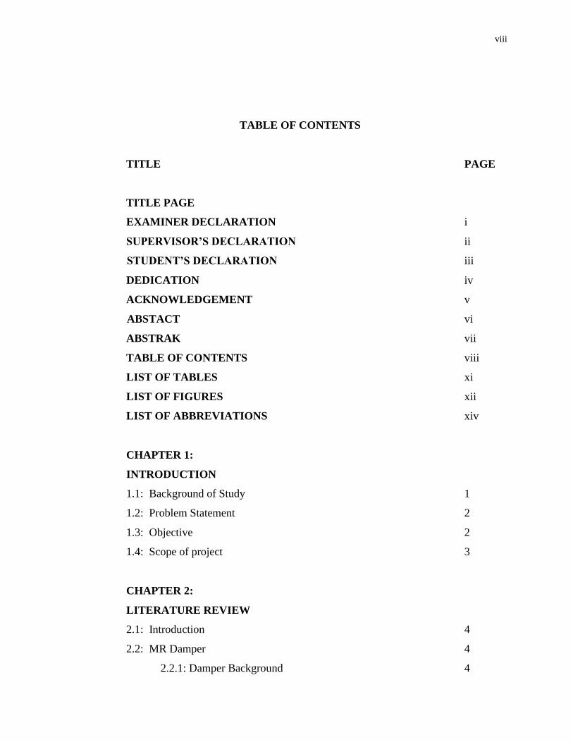
TABLE OF CONTENTS

TITLE PAGE

TITLE PAGE

EXAMINER DECLARATION i

SUPERVISOR’S DECLARATION ii

STUDENT’S DECLARATION iii

DEDICATION iv

ACKNOWLEDGEMENT v

ABSTACT vi

ABSTRAK vii

TABLE OF CONTENTS viii

LIST OF TABLES xi

LIST OF FIGURES xii

LIST OF ABBREVIATIONS xiv

CHAPTER 1:

INTRODUCTION

1.1: Background of Study 1

1.2: Problem Statement 2

1.3: Objective 2

1.4: Scope of project 3

CHAPTER 2:

LITERATURE REVIEW

2.1: Introduction 4

2.2: MR Damper 4

2.2.1: Damper Background 4

ix

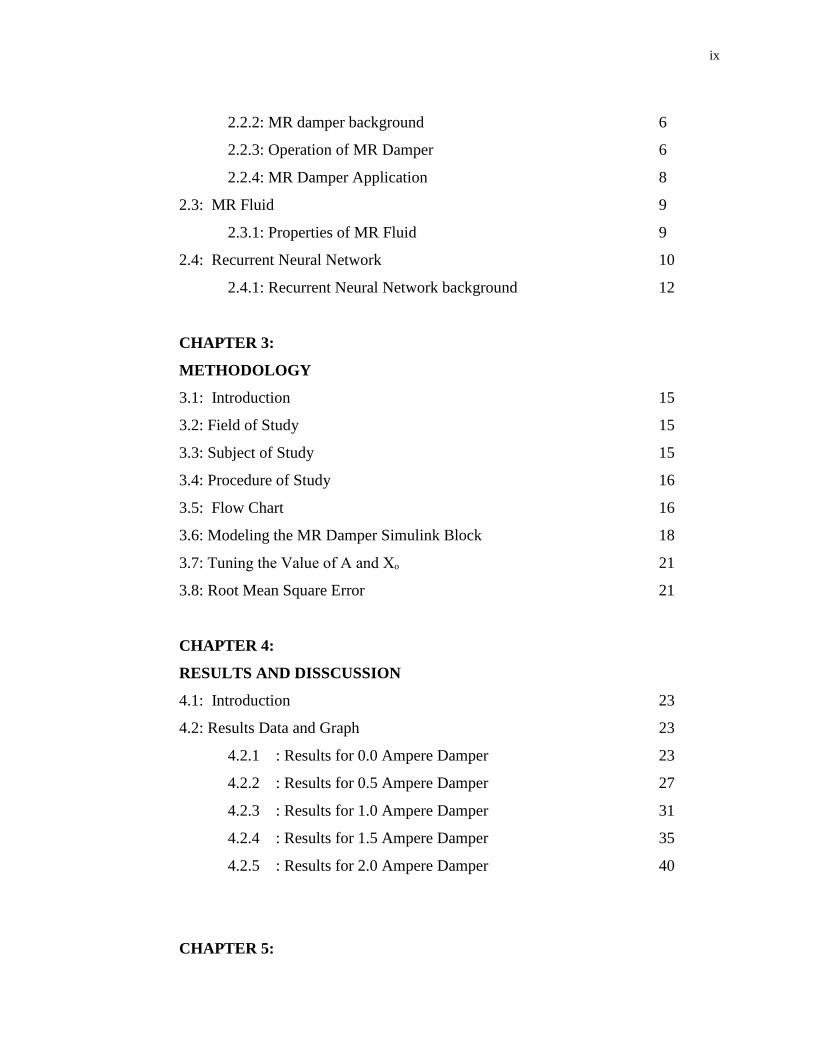
2.2.2: MR damper background 6

2.2.3: Operation of MR Damper 6

2.2.4: MR Damper Application 8

2.3: MR Fluid 9

2.3.1: Properties of MR Fluid 9

2.4: Recurrent Neural Network 10

2.4.1: Recurrent Neural Network background 12

CHAPTER 3:

METHODOLOGY

3.1: Introduction 15

3.2: Field of Study 15

3.3: Subject of Study 15

3.4: Procedure of Study 16

3.5: Flow Chart 16

3.6: Modeling the MR Damper Simulink Block 18

3.7: Tuning the Value of A and Xₒ 21

3.8: Root Mean Square Error 21

CHAPTER 4:

RESULTS AND DISSCUSSION

4.1: Introduction 23

4.2: Results Data and Graph 23

4.2.1 : Results for 0.0 Ampere Damper 23





CHAPTER 5:

x

CONCLUSION AND RECOMENDATION

5.1: Conclusion 45

5.2: Recommendation 45

REFERENCES 46

xi

LIST OF TABLES

TABLE NO. TITLE PAGE

2.1 Summary of properties of the MR fluid 10

4.1 Results for RMSE 44

xii

LIST OF FIGURES

FIGURE NO. TITLE PAGE

2.1 MR fluid damper. 6

2.2 Phenomenal behavior of the MR fluid when no magnetic 7

field applied.

2.3 Phenomenal behavior of the MR fluid when magnetic 7

field applied.

2.4 A feed forward network. 13

2.5 Simple Recurrent Neural Network. 14

3.1 Flow chart for the final year project. 17

3.2 The model simulink of the MR damper. 18

3.3 Recurrent Neural Network. 19

3.4 The coding for the output of simulink block. 20

3.5 The A and Xₒ value. 21

4.1 The simulink block for 0.0 Ampere damper. 24

4.2 Displacement graph for 0.0 Ampere damper. 24

4.3 Velocity graph for 0.0 Ampere damper. 25

4.4 Force graph for 0.0 Ampere damper. 25

4.5 The experimental damper and simulation damper 26

comparison graph 0.0 Ampere damper.

4.6 Square error graph for 0.0 Ampere damper. 26









xiii





















xiv

LIST OF ABBREVIATIONS

RNN Recurrent Neural Network

MR Magneto Rheological

ER Electro Rheological

RMSE Root Mean Square Error

1

CHAPTER 1

INTRODUCTION

1.1 BACKGROUND OF STUDY

Damper was used in most of the machine that we used every day in our daily life,

including car suspension system and clothes washing machine. The suspension system is

one of the most important parts in vehicles, while the damper is the most important part in

suspension system of the vehicles. Hit a bump without dampers, and the suspension would

continue to bounce up and down uncontrollably. The job of a car suspension is to maximize

the friction between the tires and the road surface, to provide steering stability with good

handling and to ensure the comfort of the passengers besides it also provide a safety to a

driver. For a clothes washing machine, damper function is to reduce the noise make by that

machine. In a civil engineering field, the damper was also used widely. We can saw that

damper was used widely to build the bridge and building. For a bridge, damper is so

effective to improving bridge performances. In other words, the damper could result in

simple connection and lower construction cost.

Meanwhile, for building, in order to reduce the resonance effect, it is important to

build large dampers into their design to interrupt the resonant waves. If the dampers were

not used in building, the buildings can be shaken to the ground especially when earthquake

happens.

Most of the thing used in this world is purpose to easier the human work, so are

damper. It is used because of its advantage. One of the advantage of using damper is

because, damper provide a safety for the machine or one system. For example, a building, it

2

used a damper for a safety of the people in the building. The other advantage of the damper

is to provide comfort for the user. For example, in vehicles, dampers were mostly used to

provide a comfort for the driver and passengers. Besides that, dampers also were used

because of the capability of it to reduce the cost.

There were several types of damper, one of type of damper is magnetorheological

damper or can be simplify as MR damper. A magnetorheological (MR) damper consists of

a hydraulic cylinder containing a solution that, in the presence of a magnetic field, can

reversibly change from a free flowing, linear viscous fluid to a semi-solid with controllable

yield strength. This solution is called MR fluid and is composed of micron-sized

magnetically polarizable particles dispersed in a carrier medium such as water, mineral or

synthetic oil. Typically, it contains 20 to 40% by volume of relatively pure carbonyl iron

with 3 to 5 microns in diameter (Yang, 2001). MR fluid is normally a free flowing viscous

fluid, but the presence of a magnetic field causes the particles to form chains and increase

the fluid viscosity, until it becomes a semi-solid. Additives are commonly added to

discourage settling, improve lubricity, modify viscosity, and reduce wear.

1.2 PROBLEM STATEMENT

To fulfill the objective of this project, which is to modeling the MR damper using

recurrent neural network, Besides, the input and also the updated equation in the recurrent

neural network method should been have any mistake. Besides that, MR fluid also got

unique characteristic which is it has a nonlinear characteristic. If the modeling method is

accurate the MR damper will achieve high damping control system performance.

1.3 OBJECTIVE

1) To model the magnetorheological (MR) damper.

2) To analyze the equation of simulation so that the graph of MR damper model is

almost same as theoretical damper.

3

1.4 SCOPE OF PROJECT

1) Design the model simulation of magnetorheological (MR) damper using

MATLAB software.

2) Analyze the equation of simulation using Recurrent Neural Network method.

4

CHAPTER 2

LITERATURE REVIEW

2.1 INTRODUCTION

In this chapter, the MR damper, MR fluid and the method used which is recurrent

Neural Method will be discussed. Literature study is one of the initial steps toward the

understanding of this project. The information was collected from many resources such as

journals and thesis. From this literature study, the problem statements have been noted, the

objectives of the project been set and the scope of the projects has been specified.

2.2 MR DAMPER

2.2.1 Damper background

Damper is a mechanical device that functional to flatter the impulse and to dissipate

kinetic energy. The damper in automotive consist of spring loaded check valves to control

the flow of fluid trough an internal piston. From the study of the damper, there are three

types of damper that can be concluded. The type of the damper is passive, active and the

semi- active damper.

Passive controller or passive damper is set of system that does not require a power

source to operate. The passive control dampers produce fixed design, so the damper will

not be optimal when the system or the operating condition changed. The advantages of the

passive damper are the design simplicity and cost effectiveness. Besides that, the passive

5

damper also avoided the performances limitation due to the lack of damping force

controllability.

The active control damper is a device that required a power to operate and apply

force directly into the system. The advantage of an active damper is that, it can adapt for

system variation. Besides, the active control damper also can provided high control of

performances in wide frequency range. The active control damper also can be much more

effective than the passive damper. However, the active dampers were having some lack

besides of the high power sources. The other disadvantage of the active damper is it has

many sensors and complex actuators.

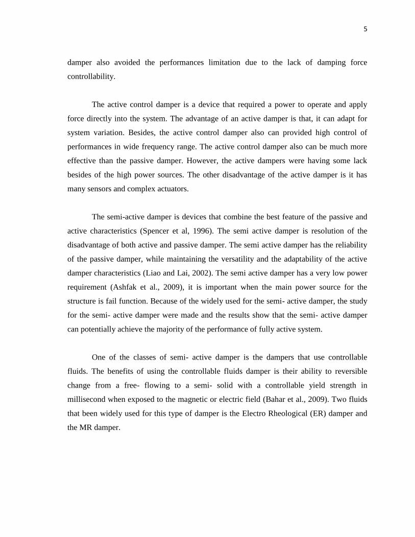
The semi-active damper is devices that combine the best feature of the passive and

active characteristics (Spencer et al, 1996). The semi active damper is resolution of the

disadvantage of both active and passive damper. The semi active damper has the reliability

of the passive damper, while maintaining the versatility and the adaptability of the active

damper characteristics (Liao and Lai, 2002). The semi active damper has a very low power

requirement (Ashfak et al., 2009), it is important when the main power source for the

structure is fail function. Because of the widely used for the semi- active damper, the study

for the semi- active damper were made and the results show that the semi- active damper

can potentially achieve the majority of the performance of fully active system.

One of the classes of semi- active damper is the dampers that use controllable

fluids. The benefits of using the controllable fluids damper is their ability to reversible

change from a free- flowing to a semi- solid with a controllable yield strength in

millisecond when exposed to the magnetic or electric field (Bahar et al., 2009). Two fluids

that been widely used for this type of damper is the Electro Rheological (ER) damper and

the MR damper.

6

2.2.2 MR damper background

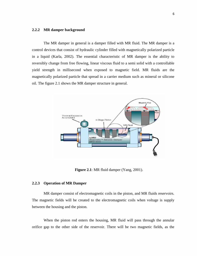
The MR damper in general is a damper filled with MR fluid. The MR damper is a

control devices that consist of hydraulic cylinder filled with magnetically polarized particle

in a liquid (Karla, 2002). The essential characteristic of MR damper is the ability to

reversibly change from free flowing, linear viscous fluid to a semi solid with a controllable

yield strength in millisecond when exposed to magnetic field. MR fluids are the

magnetically polarized particle that spread in a carrier medium such as mineral or silicone

oil. The figure 2.1 shows the MR damper structure in general.

Figure 2.1: MR fluid damper (Yang, 2001).

2.2.3 Operation of MR Damper

MR damper consist of electromagnetic coils in the piston, and MR fluids reservoirs.

The magnetic fields will be created to the electromagnetic coils when voltage is supply

between the housing and the piston.

When the piston rod enters the housing, MR fluid will pass through the annular

orifice gap to the other side of the reservoir. There will be two magnetic fields, as the

7

damper in compressed mode. The damper will resist the flow of fluid from one side to other

side of the piston when applied to magnetic field.

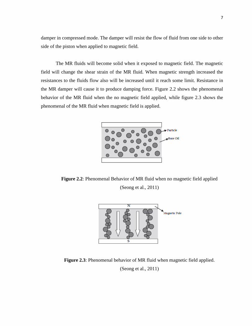
The MR fluids will become solid when it exposed to magnetic field. The magnetic

field will change the shear strain of the MR fluid. When magnetic strength increased the

resistances to the fluids flow also will be increased until it reach some limit. Resistance in

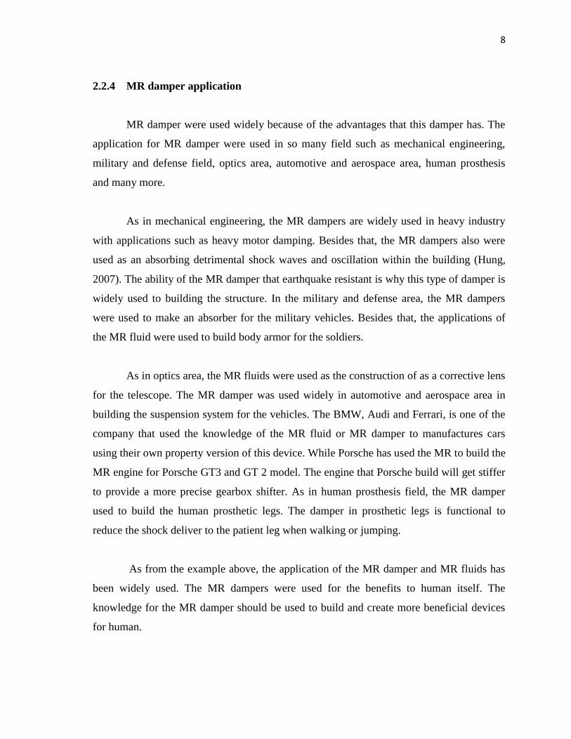
the MR damper will cause it to produce damping force. Figure 2.2 shows the phenomenal

behavior of the MR fluid when the no magnetic field applied, while figure 2.3 shows the

phenomenal of the MR fluid when magnetic field is applied.

Figure 2.2: Phenomenal Behavior of MR fluid when no magnetic field applied

(Seong et al., 2011)

Figure 2.3: Phenomenal behavior of MR fluid when magnetic field applied.

(Seong et al., 2011)

8

2.2.4 MR damper application

MR damper were used widely because of the advantages that this damper has. The

application for MR damper were used in so many field such as mechanical engineering,

military and defense field, optics area, automotive and aerospace area, human prosthesis

and many more.

As in mechanical engineering, the MR dampers are widely used in heavy industry

with applications such as heavy motor damping. Besides that, the MR dampers also were

used as an absorbing detrimental shock waves and oscillation within the building (Hung,

2007). The ability of the MR damper that earthquake resistant is why this type of damper is

widely used to building the structure. In the military and defense area, the MR dampers

were used to make an absorber for the military vehicles. Besides that, the applications of

the MR fluid were used to build body armor for the soldiers.

As in optics area, the MR fluids were used as the construction of as a corrective lens

for the telescope. The MR damper was used widely in automotive and aerospace area in

building the suspension system for the vehicles. The BMW, Audi and Ferrari, is one of the

company that used the knowledge of the MR fluid or MR damper to manufactures cars

using their own property version of this device. While Porsche has used the MR to build the

MR engine for Porsche GT3 and GT 2 model. The engine that Porsche build will get stiffer

to provide a more precise gearbox shifter. As in human prosthesis field, the MR damper

used to build the human prosthetic legs. The damper in prosthetic legs is functional to

reduce the shock deliver to the patient leg when walking or jumping.

As from the example above, the application of the MR damper and MR fluids has

been widely used. The MR dampers were used for the benefits to human itself. The

knowledge for the MR damper should be used to build and create more beneficial devices

for human.

9

2.3 MR FLUID

MR fluids, consisting of small magnetic particles dispersed in a liquid, these

material properties are controllable through the application of an external magnetic field.

Under a high magnetic field, the magnetic particles have been observed to aggregate into

elongated clusters aligned along the magnetic field direction. This macrostructure is

responsible for the solid like rheological characteristics and is hereby denoted the ground

state of the MR fluids at the high field limit. The structure of the MR fluid ground state has

been the subject of prior experimental and theoretical studies, but with conflicting

conclusions in regard to both the observations and the governing physics.

MR fluids are considerably less well known than their ER fluid. Both fluids are non

colloidal suspensions of polarizable particles having a size on the order of a few microns.

The initial discover and developer for MR fluid was Jacob Rabinow at the US National

Bureau of Standards in the late 1940s. Thanks to him, the MR fluids have enjoyed recent

commercial success. A number of MR fluids and various MR fluid-based systems have

been commercialized including an MR fluid brake for use in the exercise industry, a

controllable MR fluid damper for use in truck seat suspensions and an MR fluid shock

absorber for oval track automobile racing.

2.3.1 Properties of MR fluid

Typical magnetorheological fluids are the suspensions of micron sized,

magnetizable particles (mainly iron) suspended in an appropriate carrier liquid such as

mineral oil, synthetic oil, water or ethylene glycol. The carrier fluid serves as a dispersed

medium and ensures the homogeneity of particles in the fluid. A variety of additives

(stabilizers and surfactants) are used to prevent gravitational settling and promote stable

particles suspension, enhance lubricity and change initial viscosity of the MR fluids. The

stabilizers serve to keep the particles suspended in the fluid, whilst the surfactants are

adsorbed on the surface of the magnetic particles to enhance the polarization induced in the

suspended particles upon the application of a magnetic field.

10

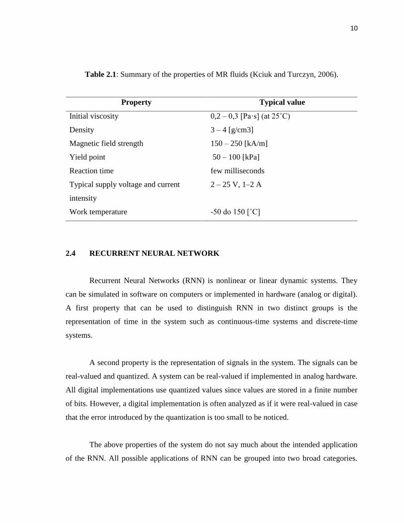
Table 2.1: Summary of the properties of MR fluids (Kciuk and Turczyn, 2006).

Property Typical value

Initial viscosity 0,2 – 0,3 [Pa·s] (at 25˚C)

Density 3 – 4 [g/cm3]

Magnetic field strength 150 – 250 [kA/m]

Yield point 50 – 100 [kPa]

Reaction time few milliseconds

Typical supply voltage and current

intensity

2 – 25 V, 1–2 A

Work temperature -50 do 150 [˚C]

2.4 RECURRENT NEURAL NETWORK

Recurrent Neural Networks (RNN) is nonlinear or linear dynamic systems. They

can be simulated in software on computers or implemented in hardware (analog or digital).

A first property that can be used to distinguish RNN in two distinct groups is the

representation of time in the system such as continuous-time systems and discrete-time

systems.

A second property is the representation of signals in the system. The signals can be

real-valued and quantized. A system can be real-valued if implemented in analog hardware.

All digital implementations use quantized values since values are stored in a finite number

of bits. However, a digital implementation is often analyzed as if it were real-valued in case

that the error introduced by the quantization is too small to be noticed.

The above properties of the system do not say much about the intended application

of the RNN. All possible applications of RNN can be grouped into two broad categories.

11

Recurrent neural networks can be used as associative memories and sequence mapping

systems. Recurrent neural networks used as sequence mapping systems are operated by

supplying an input sequence, which consists of different input patterns at each time step (in

case of a discrete time system), or a time-varying input pattern over time (in case of a

continuous-time system).At each time instant, an output is generated which depends on

previous activity of the system and on the current input pattern. The entire output sequence

generated over time is considered the result of the computation.

The class of sequence mapping systems is interesting for practical applications in

sequence recognition, generation or prediction and it will be examined in the next chapter.

Sequences mapping neural networks are nearly always implemented in software or clocked

digital hardware (both have a discrete representation of time). This report will focus on

recurrent neural networks used as sequence mapping systems. Using the common ways of

implementation these networks are discrete-time systems. Therefore, all treatment of

recurrent neural networks in the next chapters will be restricted to discrete-time systems.

Some examples of recurrent neural networks used as associative memories will be given

now.

Recurrent neural networks used as associative memories are operated by applying a

fixed input pattern (that does not change over time). Then the network is operated

according to a set of equations describing the network dynamics. Internal signals and the

network outputs will change over time. Under certain conditions (and waiting for a

sufficient time interval), the network. This means the systems output has converged to

some static pattern which is considered the result of the computation performed by the

system. This result is some association made by the system in response to the input, hence

the name associative memories.

The difference with sequence mapping systems lies in supplying a static input to the

network (not a sequence) and only using the final output values of the network as a result

(and not the output sequence over time). So both input and output are static patterns

whereas for the sequence mapping systems, both input and output are sequences.

12

These recurrent neural network architectures were proposed to create associative content

addressable memories. They were used in Artificial Intelligence research and they

contributed to research about the way the (human) brain works. Associative memories are

sometimes implemented in analog hardware, but generally for research purposes a software

implementation is favored because it is more convenient and flexible. Examples of these

architectures are the Brain-State-in-a-Box neural network and the Hopfield network. The

Hopfield network model was later on extended with neurons that operate in a stochastic

manner (using theory from the field of statistical mechanics) which are called Boltzmann

machines (Hertz et al., 1991).

2.4.1 Recurrent Neural Network background

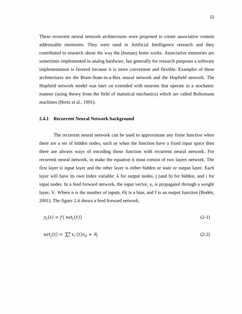
The recurrent neural network can be used to approximate any finite function when

there are a set of hidden nodes, such as when the function have a fixed input space then

there are always ways of encoding those function with recurrent neural network. For

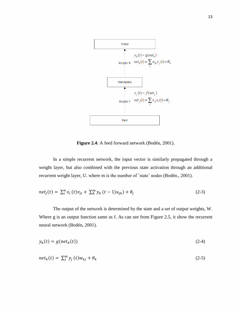
recurrent neural network, to make the equation it must consist of two layers network. The

first layer is input layer and the other layer is either hidden or state or output layer. Each

layer will have its own index variable: k for output nodes, j (and h) for hidden, and i for

input nodes. In a feed forward network, the input vector, x, is propagated through a weight

layer, V. Where n is the number of inputs, Ɵj is a bias, and f is an output function (Bodén,

2001). The figure 2.4 shows a feed forward network.

(2-1)

(2-2)

13

Figure 2.4: A feed forward network (Bodén, 2001).

In a simple recurrent network, the input vector is similarly propagated through a

weight layer, but also combined with the previous state activation through an additional

recurrent weight layer, U. where m is the number of ’state’ nodes (Bodén., 2001).

(2-3)

The output of the network is determined by the state and a set of output weights, W.

Where g is an output function same as f. As can see from Figure 2.5, it show the recurrent

neural network (Bodén, 2001).

(2-4)

(2-5)

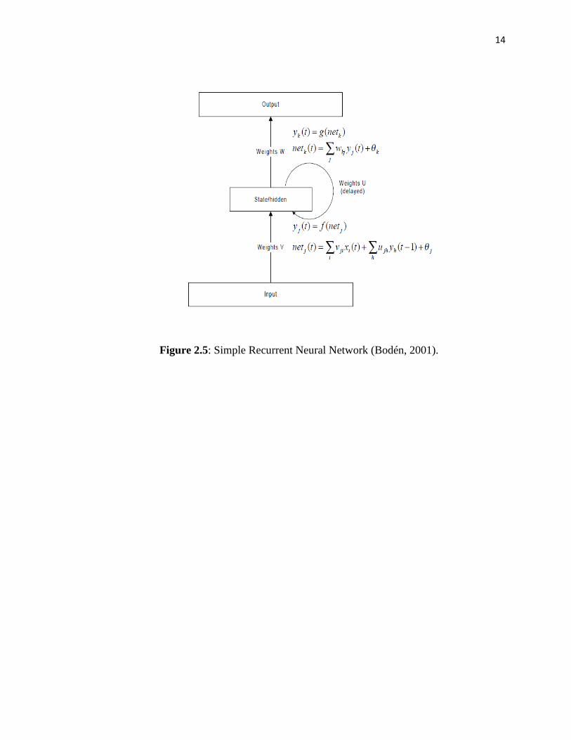
14

Figure 2.5: Simple Recurrent Neural Network (Bodén, 2001).

Documents

MODELING THE MAGNETO- RHEOLOGICAL …umpir.ump.edu.my/4426/1/cd6632_63.pdfviii table of contents title page title page examiner declaration i supervisor’s declaration ii