Modeling the Drying of Ink-Jet-Printed Structures and Experimental Verification

Modeling the Drying of Ink-Jet-Printed Structures and ExperimentalVerification

D. B. van Dam

Philips Research, High Tech Campus 4 (WAG01), 5656 AE EindhoVen, The Netherlands

J. G. M. Kuerten*

Technische UniVersiteit EindhoVen, Department of Mechanical Engineering, Section Process Technology,EindhoVen, The Netherlands

ReceiVed June 22, 2007. In Final Form: September 9, 2007

This article presents a numerical model that was developed for the drying of ink-jet-printed polymer solutions afterfilling the pixels in a polymer LED display. The model extends earlier work presented in the literature while stillmaintaining a practical approach in limiting the number of input parameters needed. Despite some rigorous assumptions,the model is in fair agreement with experimental data from a pre-pilot ink-jet printing line. Comparison inside a singlepixel is shown, as well as a general trend in which the amount of polymer that is transported out of the central partof the pixel decreases with the rate of viscosity increase as a function of polymer concentration. Moreover, the effectof a varying solute diffusion coefficient is studied.

1. Introduction

Interest in the drying of ink-jet-printed fluids appears in manydifferent fields.1-3 In the more traditional graphical applications,the visual appearance of the ink depends on the drying process,and the limitation of the total drying time is important. In newapplications of ink-jet printing, for example, for depositing electro-(optical) materials in the display and electronics industry,4 thefunctionality of the layer is of crucial importance. Thisfunctionality often depends strongly on the layer thicknessdistribution of the deposited structure. This layer thicknessdistribution in turn is determined during the drying of the layer,when a significant redistribution of material can take place. Inaddition, in multilayer devices the thickness of layers depositedon top of a printed layer depends on the geometry of the printedstructures.

The research that is described in this article was performedin the framework of an activity to manufacture polymer LEDdisplays.5 For this purpose, it is important to understand theformation of layers of light-emitting polymers with uniformthickness in predefined wells, which were formed by hydrophobicbarriers. For this application, we aimed to find a relatively simpletheoretical framework that enabled us to better guide thedevelopment of inks and of the printing process.

The drying of ink-jet-printed droplets that form thin films ofsolute is a process that can show various hydrodynamicphenomena, such as Marangoni flow and hydrodynamic instabil-ity.6 However, even in a relatively simple form that still has

practical significance, the description of the drying process alreadyposes significant difficulties. In the case considered here, themain processes involved are the convective and diffusive transportof solute, coupled with the evolution of the free surface, theevaporation of the solvent, and the viscosity increase in thesolution (Figure 1).

In previous work, the occurrence of flow and particle transportin thin fluid films is recognized, which occurs as a result of localevaporation that does not match the energetically preferred fluidsurface evolution.7,8 Significant work on the drying of dropletshas been performed by Deegan,9-11 quantifying the surface-tension-driven mechanism of convective solute transport initiatedby the evaporation of droplets with radii on the order of 1 mm.However, for smaller particles and droplets than Deegan studied,diffusion established by advectively induced concentrationgradients can become important. Also, the increase in viscosityas the concentration of the solute increases can become important.In this study, we present a practical and approximate approachtoward modeling the drying of ink-jet-printed structures contain-ing polymers or colloidal particles in which we take theseprocesses into account and compare model predictions withexperimental results.

2. Modeling Framework

Modeling should provide a description of various processes,which are the evaporation of solvent, the rheological evolutionof the ink, the advective flow field within the droplet, the diffusivetransport of solute, and the surface tension forces acting on thefluid. In the literature, several useful models were developed.The ones that we use as references are those of Deegan9-11 andFischer12 because from the existing models these come closest

* Corresponding author. E-mail: [email protected]. Phone:+31 40247 2362. Fax:+31 40 247 5399.

(1) Dufva, M. Biomol. Eng.2005, 22, 173-184.(2) Hjelt, K. T.; Van den Doel, L. R.; Lubking, W.; Vellekoop, M. J.Sens.

Actuators2000, 85, 384-389.(3) Rieger, B.; Van den Doel, L. R.; Van Vliet, L. J.Phys. ReV. E 2003, 68,

036312.(4) Bale, M.; Carter, J. C.; Creighton, C. J.; Gregory, H. J.; Lyon, P. H.; Ng,

P.; Webb, L.; Wehrum, A.SID J.2006, 14, 453-459.(5) Fleuster, M.; Klein, M.; Van Roosmalen, P.; De Wit, A.; Schwab, H.SID

Symp. Digest Tech. Pap.2004, 35, 1276.(6) Cuk, T; Trojan, S. M.; Hong, C. M.; Wagner, S.Appl. Phys. Lett.2000,

77, 2063-2065.

(7) Denkov, N. D.; Velev, O. D.; Kralchevsky, P. A.; Ivanov, I. B.; Yoshimura,H.; Nagayama, K.Langmuir1992, 8, 3183-3190.

(8) Parisse, F.; Allain, C.J. Phys. II1996, 6, 1111-1120.(9) Deegan, R. D.; Bakajin, O.; Dupont, T. F.; Huber, G.; Nagel, S. R.; Witten,

T. A. Nature1997, 389, 827-829.(10) Deegan, R. D.Phys. ReV. E 2000, 61, 475-485.(11) Deegan, R. D.Phys. ReV. E 2000, 62, 756-765.(12) Fischer, B. J.Langmuir2002, 18, 60-67.

582 Langmuir2008,24, 582-589

10.1021/la701862a CCC: $40.75 © 2008 American Chemical SocietyPublished on Web 12/11/2007

to our experimental situation, although still showing room forimprovement. In this article, we consider both viscous and inviscidmodels.

2.1. Assumptions Common to Models.We assume that thefluid is well mixed in the vertical direction. This implies that theconcentration of solute does not depend on the vertical coordinate.This assumption can be made when diffusive transport in thevertical direction is dominant over advective transport in theradial direction, which is typically the case when

whereV is a characteristic lateral flow velocity (that is largerthan the average evaporation velocity),H is a characteristic fluidlayer thickness, andD is the solute’s diffusion coefficient. Thisassumption enables us to integrate the velocity over thezcoordinate using a concentration that depends on lateralcoordinatesx andy only. (See Figure 1 for the coordinates thatwere used.)

We assume as well that surface tension gradients can beneglected. For inks with one solvent, this assumption is reasonablefor our materials because we measured no influence of soluteconcentration on surface tension. However, in inks consisting oftwo or more solvents having different evaporation velocities andsurface tension, surface tension gradients can in general beexpected. The solutal Marangoni numberM describes theproportion of the time scale for the diffusive transport of onesolvent in the other solvent and the time scale for convectivesolvent transport as a function of a surface tension gradient andcan be expressed as

whereη is the viscosity of the solution,σ is the surface tensionat the fluid-air interface,Ds is the diffusion coefficient of onesolvent in the other solvent,cs is the concentration of one solventin the ink,L is a typical size of the droplet in the lateral direction(along thex, y, or r coordinate), andRc is a typical value for theradius of curvature of the fluid-air interface. At the beginningof drying, the value ofM typically is O(1) for drying light-emitting polymer solutions (using typical values for∂σ/∂cs cs )1 × 10-3 N m-1, η ) 1 × 10-2 Pa s,Ds ) 10-9 m2 s-1, Rc )10-3 m, andH ) 1 × 10-5 m). However, as drying proceedsthe value ofH2/Rc will decrease quickly, thus justifying ourneglectance of Marangoni effects. Because the influence of solute

Marangoni effects is on the verge of being significant, it isworthwhile to consider it as a source of error when comparingexperiments with model results.

Furthermore, we assume that the contact line remains pinned,which is the case for many practical situations. This conditionis discussed by Deegan.10 By observation of the drying process,we see that this assumption also holds for our materials.

In addition, we need to specify the evaporation velocity of thefluid. For a sessile droplet with radial symmetry and radiusRof thesolid-fluid interface, theevaporationvelocity canbewrittenas11

whereVe is the evaporation rate,λ ) (π - 2θ)/(2π - 2θ), andθ is the contact angle between fluid and substrate.Ve,av is theaverage evaporation rate per unit of solid-fluid area. We assumethat the evaporation velocity is not influenced by the possiblegelation of the polymer during the drying process.

2.2. Governing Equations.The fluid flow in the droplet isgoverned by the Navier-Stokes equation and the continuityequation

whereu is the velocity vector,F is the fluid mass density,η isthe dynamic viscosity,g is the acceleration of gravity andiz isthe unit vector in the upward vertical direction. To determine therelative importance of the different terms in the governingequations, we take a typical length scaleL for the horizontal sizeof the droplet. We useH as a typical length scale for the heightof the droplet and the evaporation velocityVe,av as the typicalfluid velocity in the vertical direction. From eq 5, it follows thatthe typical velocity in the horizontal direction is equal toV )Ve,avL/H. The appropriate scale for pressure is given byσ/Rc.

Next, we decompose the fluid velocity into a horizontal anda vertical component according tou ) u | + wiz. The horizontaland vertical components of the scaled Navier-Stokes equationthen read, respectively,

and

where ∇| denotes the horizontal component of the gradientoperator and an asterisk is used for a scaled variable. Moreover,Ca is the capillary number that is defined as

We is the Weber number that is defined as

Figure 1. Schematic overview of processes incorporated in ourmodeling.

VHD

, 1 (1)

M ) ( ∂σ∂cs

cs

Rc

12ηL2

H2)(L2

Ds) ) ( ∂σ

∂cscs

12ηDs)(H2

Rc) (2)

Ve ) Ve,av(1 - λ)(1 - ( rR0

)2)-λ(3)

F∂u∂t

+ Fu‚∇u ) -∇p + η∇2u - giz (4)

∇‚u ) 0 (5)

We(∂u|/

∂t*+ u* ‚∇u|

/) ) -∇p*LRc

+ Ca(∂2u|/

∂z*2+ H2

L2∇|

2u|/) (6a)

We(∂w*∂t*

+ u* ‚∇w*) ) - ∂p*∂z*

L3

H2Rc

+

Ca(∂2w*

∂z*2+ H2

L2∇|

2w*) - Bd (6b)

Ca ) ηVσ

L2

H2(7a)

We) FV2Lσ

(7b)

Modeling the Drying of Ink-Jet-Printed Structures Langmuir, Vol. 24, No. 2, 2008583

andBd is the Bond number that is defined as

For a typical case at the start of drying,V ) 1 × 10-6 m s-1,L ) 1 × 10-4 m, H ) 1 × 10-5 m, Rc ) 1 × 10-3 m, σ ) 30× 10-3 N m-1, F ) 1 × 103 kg m-3, Ve,av ) 10-7 m s-1, andη ) 10 mPa s. Hence,We) 3 × 10-12, Ca ) 3 × 10-5, andBd ) 3 × 10-3. During the evaporation process, the viscositycan increase by 4 orders of magnitude. Hence, the capillarynumber also increases by this factor. It can be concluded that fora typical case the small Bond number and Weber number justifythe scaling of the pressure term. Moreover, it can be seen thatfor these typical magnitudes of the terms in the Navier-Stokesequation the convective terms on the left-hand side, the gravityterm, the horizontal derivatives in the viscous terms in eq 6a, andthe total viscous term in eq 6b can always be disregarded.Therefore, the governing equations reduce to

and

where for convenience the asterisks have been omitted. Theseequations are similar to those derived by Fischer12 for theaxisymmetric case, and another lubrication-based model has beenused by Routh and Russel.13 The difference is that we assumethat the viscosity depends on the solute concentration and is inthis way a function of the horizontal coordinates and time. Toshow that explicitly in eq 8b, we define

whereη0 is the viscosity at the initial solute concentration, soeq 8b can be rewritten as

For the typical parameter values mentioned above, thelubrication approximation is certainly accurate near thecenter of the droplet. Near the edge of the droplet, the estimatesfor the convective terms in the Navier-Stokes equation madeabove become more questionable because the curvature ofthe droplet interface and the substrate might become important,especially for the substrate structure considered in this article

(Figure 3a). However, even at the edge of the droplet, ofwhich the interface is given byz ) h(x, y), |∇|h| is less than 1,so the lubrication approximation remains, to good approximation,valid.

In the lubrication approximation used here, the pressure at theinterface between the droplet and surrounding air is given by

The constant on the right-hand side is on the order of unityfor typical droplets considered here. Because according to eq 8athe pressure is constant in the vertical direction, the horizontalvelocity follows from eq 10 if appropriate boundary conditionsare specified. At the bottom of the drop, the no-slip conditionu| ) 0 should hold, whereas at the interface the tangential stressbalance leads to∂u|/∂z ) 0. The solution of eq 10 is

and with eq 11 we find

In a similar way as in Fischer,12 the continuity equation canbe used to find an evolution equation for the height of the droplet

where the angular brackets denote a height average andVe is theevaporation velocity. The substitution of eq 13 finally yields(13) Routh, A. F.; Russel, W. B.AIChE J.1998, 44, 2088-2098.

Figure 2. Viscosity vs concentration for polymer ink P1.

Bd ) FgL2

σ(7c)

∂p∂z

) 0 (8a)

∇|p )Rc

LCa

∂2u|

∂z2(8b)

Ca0 )η0V

σL2

H2(9)

∇|p )Rc

Lηη0

Ca0

∂2u|

∂z2(10)

Figure 3. (a) Photoluminescence microscope view of a pixel filledwith polymer P1 and (b) schematic view of substrate geometry (notto scale).

p ) -RcH

L2∇|

2h (11)

u| )η0L

ηRcCa0(12z2 - hz)∇|p (12)

u| )η0L

ηRcCa0(12z2 - hz)∇|∇|

2h (13)

∂h∂t

) -∇|(h ⟨u|⟩) - Ve (14)

584 Langmuir, Vol. 24, No. 2, 2008 Van Dam and Kuerten

as the equation that describes the evolution of the droplet height.This equation can be solved if the viscosity is known as a functionof the horizontal coordinates. This follows from the known relationbetween viscosity and solute concentration and the convection-diffusion equation for the solute concentration:

2.3. Inviscid Approximation. For some materials, we foundthat the viscosity remains of the same order of magnitude duringthe drying process until a certain critical concentrationccr isapproached, at which the value of the capillary number using thelocal viscosity sharply increases to a value that is large comparedto unity.14 In such a case, the use of the equations derived in theprevious section makes less sense because during almost thewhole drying process the pressure term in eq 6a is completelydominant. In such a case, we use the same approach as introducedby Deegan.9

Because the pressure inside the droplet is constant, the shapeof the droplet follows from the requirement that its curvature isconstant. This leads to a unique shape if the volume of the dropletand the shape of the contact line are known. In this work, weassume that the contact line is pinned and the volume of thedroplet follows from the known evaporation velocity profileintegrated over the interface. To solve eq 16 for the soluteconcentration, the height-averaged velocity has to be known.Equation 14 still holds but is not sufficient to determine the fluidvelocity if the droplet is not axisymmetric. An additional equationis found by averaging eq 12 over the droplet height. This resultsin15

The convection-diffusion equation (eq 16) for the soluteconcentration is used to calculate the time evolution of the soluteconcentration, but the concentration and local solute transportare limited to the critical concentrationccr.

When we assume a radial geometry of the droplet, the conditionof constant curvature reduces to the condition that a sphericalcap is always maintained. The thickness of the fluid layer is thengiven by

We can also infer that the problem is described by threedimensionless numbers and a parameter describing the evapora-tion rate profile

whereH0, R0, and λ0 are the central layer thickness, dropletradius, andλ at the start of drying.

2.4. Numerical Method.In both the viscous approach and theinviscid approximation, eq 16 is discretized with a finite volumemethod on a structured grid using second-order accurate centraldifferences for the diffusion terms and a first-order accurateupwind method for the convective terms. Integration in time isperformed by the second-order accurate implicit Crank-Nicolsonmethod. Because the equation is linear in concentration and thediscretization uses only nearest neighbors, the linear system ofequations can be solved by a direct method.

In the viscous approach, the evolution equation for the height(eq 15) is discretized in space with a second-order accurate finitevolume method in space. For integration in time, a method basedon the trapezoidal rule and especially suited for stiff systems isused. Because the equation is highly nonlinear, the time step hasto be restricted to a small value.

In the inviscid approximation, the equation that determinesthe shape of a surface with constant curvature and a given volumeis discretized on a structured grid with second-order accuratecentral differences. In the lubrication approximation, the equationis linear and is solved by a direct method. If the droplet heightis known, then the governing equations for the height-averagedhorizontal fluid velocity are also linear and are solved in thesame way.

3. Experimental Method and Materials

3.1. Materials Used.The light-emitting polymers were all obtainedin solution, from various suppliers. A number of different kinds ofpolymers and solvents were used. The average molecular weight ofall polymers was around 3× 105 daltons. The solutions containedone, two (in most cases), or three organic solvents. The mix ofpolymer and solvents was tailored to have a viscosity of 10 mPa s,measured at a shear rate of about 102 s-1. These solvent-polymercombinations were evaluated during the ink development processwhen aiming for a flat polymer layer after drying while at the sametime the various specifications for processability had to be met. Acombination of two solvents with different evaporation rates andsolubility for the polymer in general facilitates the achievement ofa relatively flat polymer layer after drying.16

In this article, we present a direct comparison between measuredpolymer layer thicknesses in an experiment using polymer ink P1and in our numerical simulations. Polymer ink P1 is based onm-xylene and decalin (1:1 cis/trans mixture) in a weight proportionof 40:60 and a green-light-emitting polymer with an averagemolecular weight of 3×105daltons. The initial polymer concentrationfor this ink is 1.1 wt %.

3.2. Material Characterization. For different inks, differencesin polymer, its molecular weight distribution, and solvents are allrepresented by differences in the measured shear viscosity as afunction of polymer concentration. For the light-emitting polymerinks, the expected evolution of shear viscosity during evaporationwas measured in a cone-plate rheometer. The samples at higherconcentration thanc0 were obtained in two ways. First, the polymersolute was partially evaporated in a thin film evaporator. Sampleswere taken at different concentrations, and in this way a curve ofpolymer concentration versus shear viscosity was obtained. Second,expected concentrations of solvents during evaporation werecalculated. Then, polymer solutions with the relevant proportionsof solvents were made, and the viscosity of these solutions wasmeasured. Figure 2 shows the results for ink P1, for which thesamples were obtained by the thin-film evaporation method. Theviscosity was determined at a shear rate of about 0.1 s-1, which isrepresentative of the conditions during drying.

The diffusion coefficient of a number of polymers was measuredwith NMR, using the ink before evaporation took place. From eightdifferent inks based on a range of polymers and solvents, the diffusion

(14) van Dam, D. B. InMechanics of the 21st Century: Proceedings of the21st International Congress of Theoretical and Applied Mechanics; Gutkowski,W., Kowalewski, T. A., Eds.; Springer: Dordrecht, The Netherlands, 2005.

(15) Popov, Y. O.; Witten, T. A.Phys. ReV. E 2003, 68, 036306.(16) Lyon, P. J.; Carter, J. C.; Bright, C. J.; Cacheiro, M. WO 02/069119 A1,

2002.

∂h∂t

)η0L

3RcCa0∇|(h3

η∇|∇|

2h) - Ve (15)

∂

∂t(ch) + ∇|(c⟨u|⟩h) ) ∇|(Dh∇|c) (16)

∇|

η⟨u|⟩

h2) 0 (17)

h ) x(R02 + hr)0

2

hr)02 )2

- r2 - (R2 - hr)02

2hr)0 ) (18)

NH )H0

R0ND )

H0D

Ve,avR02

Nc )c0

ccrλ0 (19)


coefficients were found to be between 0.4× 10-11 m2 s-1 and 1.3× 10-11 m2 s-1. For an ink that resembles the P1 ink (containingthe same polymer and based on a 70:30 mixture ofm-xylene/decalin),the diffusion coefficient of the polymer was (4.7( 0.5)× 10-12 m2

s-1. The diffusion coefficient ofm-xylene in this ink was measuredto be (1.1( 0.1) × 10-9 m2 s-1.

An accurate assessment of the evaporation rate during dryingis rather complicated. First, the drying conditions during theprinting process are strongly dependent on the local flow conditions.These conditions depend on such factors as the geometry of theexperimental setup and the air flow setting of the fume hood inwhich the experiments are conducted. The printed pattern is importantas well because the total evaporation rate of a small structureand its distribution over the surface of that structure are in generaldependent on the size of the structure and on the presence ofother fluid structures in the vicinity. In this study, we took thepragmatic approach to assessing the evaporation time from the totaldrying time of the printed plate, which was several minutes. Becausethe average layer thickness is approximately 10µm, we estimatethe average evaporation rate to be between 1× 10-7 and 1× 10-8

m s-1. Simulations are done for both values of the evaporationrate. Because the pixel containing the printed fluid is surrounded bymany other filled wells, we assume that the evaporation rate isindependent of the position in the pixel. If the pixel shape hadbeen axisymmetric, then this would have corresponded toλ ) 0 ineq 3. This approach also denies the multisolvent character of theink, which leads to evaporation rates that vary in position andtime.

3.3. Experimental Setup and Method.The drying data of thelight-emitting polymers were obtained from samples that were ink-jet printed on an experimental pre-pilot line, where inks and printheads were changed regularly. In this line, two types of multinozzleprint heads were used as obtained from Spectra. These types werethe Spectra Galaxy head (256 nozzles) and the Spectra SX head (128nozzles), which use piezoelectric actuation of the fluid. Glasssubstrates with dimensions of 15 cm× 15 cm were used, and theycontained photolithographically defined Novolak structures. Thesubstrates were cleaned using O2 plasma, and subsequently CF4

plasma treatment was applied, which preferentially made the organicstructures on the substrate hydrophobic. In this way, a contrast insurface energy was reached that enabled us to contain the printedfluid effectively within the organic structures (referred to as wellsor pixels). During printing and drying, the substrates were restingon a metal chuck that was kept at 30°C. In addition, the substratesexperienced rather strong airflow in order to remove the harmfulsolvent vapor. After printing, an∼60 nm thin aluminum layer isdeposited by evaporation on top of the substrate. Afterward, thesurface shape is measured using white-light interferometry. Theempty pixels are used for reference to determine the absolute valueof the layer thickness.

Figure 3a shows an optical micrograph of the substrate, withsome pixels filled with polymer. The pixels have a pseudoellip-tical shape. Figure 3b shows a schematic cross section along theminor axis of the pixel. It shows the geometry and lateral length ofthe SiO layer (250 nm thickness) and the Novolak resist structure(top height of about 2.5µm). These structures are similar along themajor axis of the ellipse, where the lateral distance from the top ofthe resist structure to the center of the pixel is 92.5µm. These arethe designed dimensions, but the real distances can be slightlydifferent. In the numerical model, the edge of the SiO layer isperpendicular to the substrate. In reality, however, the edge issomewhat tapered.

4. Results of Experiments and Simulations

4.1. Comparison of Various Models.For the specific pixelgeometry, Figure 4 shows a comparison of the viscous andthe inviscid model. In the viscous simulation, the followinginput parameters are used: the initial volume of the droplet is82 pL,D ) 0 m2 s-1, Ve,av) 10-7 m s-1, and the viscosity curvefrom Figure 2 is used. The evaporation rate is independent

of position and constant in time. For the inviscid simulation,we have to determine a critical dimensionless concentrationccr/c0 above which the transport of polymer effectively stops.To estimateccr/c0, we consider the proportion of the pressureterm and the viscous term in eq 6a. We can then estimateccr/c0

by determining the viscosity at whichCa Rc/L is O(1).From geometrical considerations, we can deduce thatRc/L )L/2H when H2 , L2 for a surface in the form of a sphericalcap. Assuming thatL/H ) 10, σ ) 0.03 N m-1, andV ) 10-6

m s-1, we find that forη ) O(102), Ca Rc/L is about O(1).From Figure 2, we can now determine the value ofccr/c0 to be1.84.

Significant differences can be observed in Figure 4. The inviscidmodel in general predicts less polymer in the center than doesthe viscous model. This example is representative of thecomparison between viscous and inviscid simulations in general.Another striking difference is the sharp peak in polymer thicknessalong the straight edges of the pixel in the viscous simulation.This peak becomes less pronounced for higher values of theevaporation rate (Figure 5). Although in some experiments similarsharp peaks in polymer thickness have been observed, thesepeaks are partially due to incomplete physical modeling. Duringevaporation of the droplet, the solute concentration keeps growingnear the edges of the droplet. Therefore, in the numerical modela maximum solute concentration, corresponding to close packing,is introduced, after which the convection of the solute is stopped.A decrease of this maximum solute concentration results in areduction of the observed peak in polymer height but has anegligible influence on the polymer thickness away from theedge of the droplet.

4.2. Comparison with Experiment.Figure 3a gives typicalexamples of printed pixels using polymer ink P1. On average,the contact line of the ink is positioned at 30% of the totalwidth of the resist structure. Figure 5 shows the comparison

Figure 4. Comparison between the inviscid (top) and viscous(bottom) models. The colors indicate the height of the polymer layer.


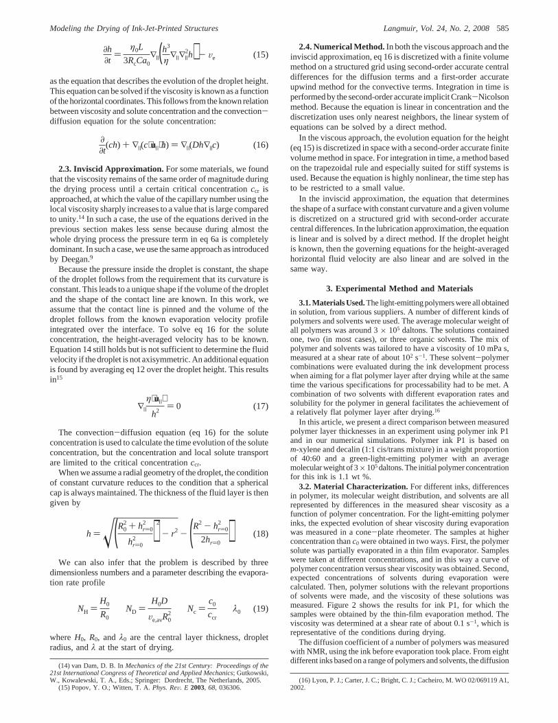
between experimental and simulated layers for ink P1. Four curvesare calculated. First, there is the inviscid model usingccr/c0 )1.84. Second and third, there are results of the viscous modelwith two evaporation rates that are constant over the whole pixel.In these three calculations, the diffusion coefficientD equalszero. Fourth, there is the result of the viscous model using thelower evaporation rate of 10-8 m s-1 and a diffusion coefficientequal to 4.7× 10-12 m2 s-1 that is independent of polymerconcentration.

To make a comparison between experiment and simulation,a value for the density of the printed layerFdry after drying hasto be assumed. We choose this value such that the simulatedcurve that includes diffusion and the experimental measurementsin Figure 5 have the same layer thickness in the center of thepixel. This yields a value ofFdry equal to 1.05× 103 kg m-3,which appears to be realistic. In calculating this value, we useda density of ink equal to 0.88× 103 kg m-3.

Going from the center of the pixel toward the edge along theminor axis, the SiO and resist structures are present atx/X0 )0.61 and 0.81. Along the major axis of the pixel, these are locatedat y/X0 ) 1.95 and 2.15. These positions give rise to numericalinaccuracies because the droplet height in eq 16 is discontinuous,which causes fluctuations in the calculated layer thickness. Forvalues ofx/X0> 0.61 andy/X0> 1.95, a good comparison betweenexperiment and simulation is not possible. At these positions,the polymer rests on top of the SiO layer and/or resist structure.Because the thickness of these layers can vary somewhat and issignificantly larger than the polymer layer thickness, the polymerlayer thickness cannot be accurately inferred from the measuredprofile.

A comparison between the experiment with ink P1 and thesimulations shows that most experimental features are reproducedin the simulations, that is, the convex shape in the center and theslight increase atx/X0 ≈ 0.5 that appears to be related to thepresence of diffusion. However, the increase in the measuredlayer thickness at 1.5< y/X0 < 1.95 is not visible in thesimulations.

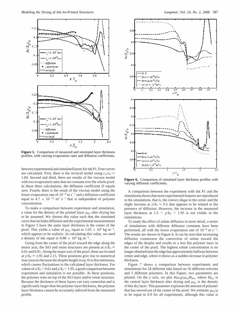
To study the effect of solute diffusion in more detail, a seriesof simulations with different diffusion constants have beenperformed, all with the lower evaporation rate of 10-8 m s-1.The results are shown in Figure 6. It can be seen that increasingdiffusion counteracts the convection of solute toward theedges of the droplet and results in a less flat polymer layer inthe center of the pixel. The highest solute concentration is nolonger obtained near the edge but approximately halfway betweencenter and edge, where it shows as a sudden increase in polymerthickness.

Figure 7 shows a comparison between experiments andsimulations for 24 different inks based on 16 different solventsand 5 different polymers. In this Figure, two parameters areplotted. On they axis, we plotH0c0F/FdryHdry, whereHdry isthe central layer thickness after drying andFdry is the densityof this dry layer. This parameter expresses the amount of polymerthat has moved out of the center of the pixel. We estimateFdry/Fto be equal to 0.9 for all experiments, although this value is

Figure 5. Comparison of measured and simulated layer thicknessprofiles, with varying evaporation rates and diffusion coefficients.

Figure 6. Comparison of simulated layer thickness profiles withvarying diffusion coefficients.


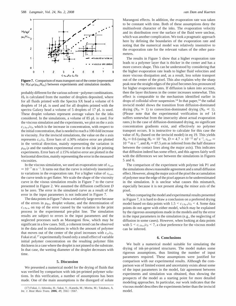
probably different for the various solvent-polymer combinations.H0 is calculated from the number of droplets deposited, wherefor all fluids printed with the Spectra SX head a volume of 6droplets of 14 pL is used and for all droplets printed with thespectra Galaxy head a volume of 5 droplets of 17 pL is used.These droplet volumes represent average values for the inksconsidered. In the simulations, a volume of 85 pL is used. Forthe viscous simulation and the experiments, we plot on thexaxisc1 Pa s/c0, which is the increase in concentration, with respect tothe initial concentration, that is needed to reach a 100-fold increasein viscosity. For the inviscid simulations, the value on thex axisrepresentsccr/c0. Error bars of(30% relative error are plottedin the vertical direction, mainly representing the variation inFdry/F and the random experimental error in the ink jet printingexperiments. Error bars of(15% relative error are plotted in thehorizontal direction, mainly representing the error in the measuredviscosities.

In the viscous simulation, we used an evaporation rate ofVe,av

) 10-7 m s-1. It turns out that the curve is relatively insensitiveto variations in the evaporation rate. For a higher value ofVe,av,the curve tends to get flatter. We scale the shape of the viscositycurve in the visous simulation results in Figure 7 to the curvepresented in Figure 2. We assumed the diffusion coefficientDto be zero. The error in the simulated curve as a result of theerror in the input parameters is not indicated in Figure 7.

The data points in Figure 7 show a relatively large error becauseof the errors inFdry, droplet volume, and the determination ofc1 Pa s, on top of the error caused by the variation in the printprocess in the experimental pre-pilot line. The simulationresults are subject to errors in the input parameters and theneglected processes such as Marangoni flow, which may besignificant in a few cases. Still, a coherent trend can be observedin the data and in simulations in which the amount of polymerthat moves out of the center of the pixel increases withccr/c0.Fukai et al.17experimentally found only a small effect of variableinitial polymer concentration on the resulting polymer filmthickness in a case where the droplet is not pinned to the substrate.In that case, the wetting diameter of the droplet decreases withtime.

5. Discussion

We presented a numerical model for the drying of fluids thatwas verified by comparison with ink-jet-printed polymer solu-tions. In this verification, a number of assumptions has beenmade. One of the main assumptions is the disregard of solute

Marangoni effects. In addition, the evaporation rate was takento be constant with time. Both of these assumptions deny themultisolvent character of the inks. The evaporation velocityand its distribution over the surface of the fluid were unclear,which was another complication. We took a pragmatic approachhere by defining the boundaries of the evaporation rate andnoting that the numerical model was relatively insensitive tothe evaporation rate for the relevant values of the other para-meters.

The results in Figure 5 show that a higher evaporation rateleads to a polymer layer that is thicker in the center and has amore convex shape. This can be understood by considering thatthe higher evaporation rate leads to higher fluid velocities andmore viscous dissipation and, as a result, less solute transportout of the center of the pixel. This also explains why the sharppeak near the straight edges of the pixel becomes less pronouncedfor higher evaporation rates. If diffusion is taken into account,then the layer thickness in the center increases somewhat. Thiseffect is comparable to the mechanism identified earlier indrops of colloidal silver suspension.14 In that paper,14 the radialinviscid model shows the transition from diffusion-dominateddrying (ND . 1) to convection-dominated drying (ND , 1).(Please note that the experimental verification in ref 14suffers somewhat from the insecurity about actual evaporationrates.) In the case of diffusion-dominated drying, no significantconcentration gradients exist, and effectively no polymertransport occurs. It is instructive to calculate for this case thevalue ofND (based on the inviscid model) in eq 19. This yieldsND ) 0.6 (usingH0 ) 10-5m, D ) 4.7× 10-12 m2 s-1, Ve,av)10-8 m s-1, andR0 ) 87.5µm as inferred from the half distancebetween the contact lines along the major axis). This indicatesthat diffusion indeed has some effect, and this agrees fairly wellwith the differences we see between the simulations in Figures5 and 6.

The comparison of the experiment with polymer ink P1 andthe simulations shows reasonable agreement and a small diffusioneffect. However, along the major axis of the pixel the accumulationof polymer near the edge of the pixel appears to be underestimatedin the simulation. It is unclear what causes this mismatch,especially because it is not present along the minor axis of thepixel.

When comparing the model and experimental results presentedin Figure 7, it is hard to draw a conclusion on a preferred dryingmodel based on data points with 1.5< c1 Pa s/c0 < 4. Some datapoints do not agree with either model, which may be explainedby the rigorous assumptions made in the models and by the errorin the input parameters in the simulation (e.g., the neglecting ofdiffusion in some cases). However, when looking at data pointswith 5 < c1 Pa s/c0 < 7, a clear preference for the viscous modelcan be inferred.

6. Conclusions

We built a numerical model suitable for simulating thedrying of ink-jet-printed structures. The model makes somerigorous assumptions, thus limiting the number of inputparameters required. These assumptions were justified forcomparison with our experimental results. Although the com-parison was of limited extent and uncertainty exists about someof the input parameters in the model, fair agreement betweenexperiments and simulation was obtained, thus showing theprospects of the model as a starting point for more detailedmodeling approaches. In particular, our work indicates that theviscous model describes the experiments better than the inviscidmodel.

(17) Fukai, J.; Ishizuka, H.; Sakai, Y.; Kaneda, M.; Morita, M.; Takahara, A.Int. J. Heat Mass Trans.2006, 49, 3561-3567.

Figure 7. Comparison of mass transport out of the center (representedby H0c0F/FdryHdry) between experiments and simulation models.


In our opinion, the current model presents a good compromisebetween complexity on the one hand and usability in an industrialenvironment on the other hand. The model prediction can beused to steer the basics of ink development. In addition, it canbe extended relatively easily to include more material properties,if necessary, or to change the evaporation rate during thesimulation to represent the multisolvent character of an ink.

Acknowledgment. We thank Roland van de Molengraaf forthe NMR measurements, Martin Hack for the viscosity measure-ments, Harry Nulens for the measurement of the layer thickness,and Dirk Roos and Willem Huugen for performing the printingexperiments. J.G.M.K. thanks Philips Research for their hos-pitality during his stay there.

LA701862A


Documents

Modeling the Drying of Ink-Jet-Printed Structures and Experimental Verification