Seediscussions,stats,andauthorprofilesforthispublicationat:https://www.researchgate.net/publication/267634610

Modelingsurfacewater-groundwaterinteractioninaridandsemi-aridregionswithintensiveagriculture

ARTICLEinENVIRONMENTALMODELLINGANDSOFTWARE·JANUARY2015

ImpactFactor:4.42·DOI:10.1016/j.envsoft.2014.10.011

CITATIONS

7

READS

432

6AUTHORS,INCLUDING:

YongTian

SouthUniversityofScienceandTechnolog…

16PUBLICATIONS60CITATIONS

SEEPROFILE

yiZheng

PekingUniversity

23PUBLICATIONS209CITATIONS

SEEPROFILE

BinWu

PekingUniversity

7PUBLICATIONS49CITATIONS

SEEPROFILE

ChunmiaoZheng

UniversityofAlabama

205PUBLICATIONS3,729CITATIONS

SEEPROFILE

Allin-textreferencesunderlinedinbluearelinkedtopublicationsonResearchGate,

lettingyouaccessandreadthemimmediately.

Availablefrom:yiZheng

Retrievedon:29January2016

lable at ScienceDirect

Environmental Modelling & Software 63 (2015) 170e184

Contents lists avai

Environmental Modelling & Software

journal homepage: www.elsevier .com/locate/envsoft

Modeling surface water-groundwater interaction in arid andsemi-arid regions with intensive agriculture

Yong Tian, Yi Zheng*, Bin Wu, Xin Wu, Jie Liu, Chunmiao ZhengCenter for Water Research, College of Engineering, Peking University, Beijing 100871, China

a r t i c l e i n f o

Article history:Received 10 March 2014Received in revised form10 October 2014Accepted 13 October 2014Available online

Keywords:Surface water-groundwater interactionIntegrated modelingGSFLOWSWMMHeihe River Basin

* Corresponding author.E-mail address: yizheng@pku.edu.cn (Y. Zheng).

http://dx.doi.org/10.1016/j.envsoft.2014.10.0111364-8152/© 2014 Elsevier Ltd. All rights reserved.

a b s t r a c t

In semi-arid and arid areas with intensive agriculture, surface water-groundwater (SW-GW) interactionand agricultural water use are two critical and closely interrelated hydrological processes. However, theimpact of agricultural water use on the hydrologic cycle has been rarely explored by integrated SW-GWmodeling, especially in large basins. This study coupled the Storm Water Management Model (SWMM),which is able to simulate highly engineered flow systems, with the Coupled Ground-Water and Surface-Water Flow Model (GSFLOW). The new model was applied to study the hydrologic cycle of the ZhangyeBasin, northwest China, a typical arid to semi-arid area with significant irrigation. After the successfulcalibration, the model produced a holistic view of the hydrological cycle impact by the agricultural wateruse, and generated insights into the spatial and temporal patterns of the SW-GW interaction in the studyarea. Different water resources management scenarios were also evaluated via the modeling. The resultsshowed that if the irrigation demand continuous to increase, the current management strategy wouldlead to acceleration of the groundwater depletion, and therefore introduce ecological problems to thisbasin. Overall, this study demonstrated the applicability of the new model and its value to the waterresources management in arid and semi-arid areas.

© 2014 Elsevier Ltd. All rights reserved.

Software availability

Name: GSFLOW-SWMMProgram language: Fortran and CDevelopers: Dr. Yong Tian (yongtian@pku.edu.cn) and Dr. Yi Zheng

(yizheng@pku.edu.cn), Center forWater Research, Collegeof Engineering, Peking University, Beijing 100871, China

Availability: Contact the developers

1. Introduction

In arid and semi-arid regions, interaction between surface water(SW) and groundwater (GW) plays an important role in the eco-hydrological system (Sophocleous, 2002; Gilfedder et al., 2012).The interaction is often complicated by agricultural activitiesincluding surface water diversion, groundwater pumping and irri-gation, as they could significantly alter the flow regimes of bothsurface water and groundwater (Barlow et al., 2000; McCallumet al., 2013; Shah, 2014; Siebert et al., 2010). Understanding thecomplex behavior of the integrated SW-GW system is very

important to the regional water resources management (Rassamet al., 2013), and integrated modeling is a highly desired approach.

A number of integrated SW-GW models have been developed,such as GSFLOW (Markstrom et al., 2008), HydroGeoSphere(Brunner and Simmons, 2012; Therrien et al., 2010), ParFlow(VanderKwaak and Loague, 2001), MIKE SHE (Graham and Butts,2005), MODHMS (Panday and Huyakorn, 2004) and SWATMOD(Sophocleous et al., 1999). Some of these models incorporateMODFLOW (Harbaug, 2005), a classic 3-D groundwater simulator,as their subsurface module. For example, GSFLOW integrates Pre-cipitation Runoff Modeling System (PRMS) (Leavesley et al., 1983)with MODFLOW; SWATMOD couples the widely applied Soil WaterAssessment Tool (SWAT) (Arnold et al., 1998) model with MOD-FLOW; and MODHMS introduces 2-D diffusion wave routing forsurface water into MODFLOW. The existing models have beenapplied to address different water resources issues, including irri-gation management (e.g., P�erez et al., 2011), SW-GW interactions(e.g., Huntington and Niswonger, 2012; Niswonger et al., 2008;Werner et al., 2006), land use and climate change (e.g., Grahamand Butts, 2005; Markstrom, 2012), water quality (e.g., Borah andBera, 2003) and so on.

However, few studies (Demetriou and Punthakey, 1998) haveinvestigated the hydrologic impacts of agricultural water use in thecontext of integrated SW-GW modeling, especially for large river

Y. Tian et al. / Environmental Modelling & Software 63 (2015) 170e184 171

basins. The lack of research is in part due to the limited capacity ofthe existing integrated models in simulating the complicated flowregime in an irrigation system. For example, unlike a natural rivernetwork inwhich tributaries run into themain stream, an irrigationnetwork has a main aqueduct which splits water into lower-orderaqueducts. Also, engineering structures (e.g., culverts, weirs,gates, and pumps) and their operations in irrigation systems areoften ignored by the existing models. Hydraulic modules in thecurrent models are not able to handle these complexities. On theother hand, some studies (Rassam, 2011; Rodriguez et al., 2008;Valerio et al., 2010; Welsh et al., 2013) introduced advanced hy-draulic engines (e.g., HEC-RAS, RiverWare, SIMS) into MODFLOW,but the basin-scale SW-GW interaction was not fully accounted for.

To better address the role of agricultural water use in integratingSW-GW modeling, this study coupled GSFLOW with SWMM(Rossman, 2009). To our best knowledge, this coupling has not beenattempted by previous studies. SWMM is a dynamic and distrib-uted model for simulating runoff quantity and quality. It has beenwidely used to study different rainfall-runoff issues (Giron�as et al.,2010; Peterson andWicks, 2006; Shrestha et al., 2013). Its hydraulicengine can nicely handle the flow in artificial waterways withdifferent engineering structures. GSFLOW's strength in modelingSW-GW interaction and SWMM's strength in hydraulic simulationcomplement each other. In addition to the coupling, two moduleswere added, one to allocate diverted water from aqueducts tofarms, and the other to allocate pumped water fromwells to farms.

The coupledmodel (hereafter called GSFLOW-SWMM)was thenapplied to Zhangye Basin (ZB), a typical arid and semi-arid area innorthwest China. ZB is the mid-stream part of Heihe River Basin(HRB), which is the second largest inland river basin in China. TheSW-GW interaction in ZB is significant and complicated (Hu et al.,2007), and highly impacted by agricultural irrigation which con-sumes a great amount of water from the Heihe River and localaquifers. Securing the environmental flow towards the down-stream has been an important management issue, due to the fastdegradation of the ecosystem in the lower HRB (the Gobi Desertarea) and the shrink of the terminal lake, the Juyan Lake (Guo et al.,2009). Hydrological modeling has been performed for both theentire HRB and ZB alone (Li et al., 2013, 2010; Wang et al., 2010;Wen et al., 2007; Zhang et al., 2004), but fully integrated SW-GWmodeling has not been attempted for this area.

Overall, this studywas aimed to: 1) enhance the capability of theintegrated SW-GW modeling in addressing highly engineered flowsystems such as the agricultural irrigation system; and 2) demon-strate how the integrated modeling would benefit the hydrologicalprocess understanding and water resources management at largebasins. In the remaining of this paper, Section 2 introduces thecoupling strategy and additional modules added. Section 3 de-scribes the study area and the modeling procedure. Results anddiscussion are presented in Sections 4, and conclusions are pro-vided in Section 5.

2. Modeling framework

2.1. Introduction to GSFLOW and SWMM

GSFLOW (Coupled Ground-Water and Surface-Water FlowModel) is a model developed by USGS (Markstrom et al., 2008)which simulates all major processes of the hydrologic cycle. It in-tegrates PRMS with MODFLOW which perform surface hydrologysimulation and 3-D groundwater simulation, respectively. TheMODFLOW2005 version adopts the UZF package (Niswonger et al.,2006) as its unsaturated-zone flow simulation module, the SFR2package (Niswonger and Prudic, 2005) as its streamflow module,and the WELL package to account for groundwater pumping. In the

PRMS domain, GSFLOW delineates the study area into hydrologicresponse units (HRUs), with the aid of external tools such asArcSWAT. HRUs can be grouped into sub-basins, and each sub-basincontains one “river segment”. The delineation of the subsurfacedomain follows the standard procedure of MODFLOW. The portionof the river segment within a MODFLOW grid is referred to as a“reach”. A river segment usually consists of multiple reaches.GSFLOWgenerally runs at a daily time step, but its SFR2 componentcan take sub-daily time steps (e.g., hourly). GSFLOW defines“gravity reservoir” as a storage in which an HRU exchanges waterwith the MODFLOW grid(s) it intersects. In reaches where streamwater is connected with groundwater, the stream-aquifer exchangeis calculated based on the head difference using Darcy's law. Moredetails about GSFLOW can be found in Markstrom et al. (2008).

SWMM conceptualizes four compartments including atmo-sphere, land surface, groundwater and transport (i.e. drainagenetwork). In the model, precipitation is transferred from atmo-sphere to land surface, and then either is delivered as runoff to thetransport compartment or infiltrates into groundwater. Thegroundwater compartment is segmented into upper unsaturatedzone and lower saturated zone. Water fluxes leaving the two zonesincluding evapotranspiration (ET), lateral interflow to the transportcompartment, and percolation to deep groundwater, which arecalculated by the model. A simple mass balance calculation isapplied to determine the storage change. SWMM uses a node-linkscheme to represent a drainage network. A link controls the rate offlow from one node to another. Links are typically conduits (openchannels and pipes), but can also be orifices, weirs or pumps. Anode accepts runoff from the sub-catchment it links. Tributaryflows, inflows or diversions could also be specified for nodes. Thereare four types of nodes in SWMM, junction, divider, outfall andstorage unit. A junction is a connection where links join together.Dividers are drainage system nodes that divert inflows to a specificconduit in a prescribed manner. Outfalls are terminal nodes of thedrainage network used to define downstream boundaries. Storageunits provide water storage capacities at specific locations.

SWMM has an advanced hydraulic simulation engine, which isable to handle large-size drainage networks and simulate compli-cated flow regimes (e.g., backwater, reverse flow, etc.). It can alsosimulate various hydraulic structures and their operations. Theengine employs finite difference method to solve one-dimensionalSainteVenant equations, either using kinematic wave (KW)method or dynamic wave (DW) method. The time and spatial res-olutions for the hydraulic calculation vary, and could be determinedbased on the courant condition. SWMM allows stand-alone hy-draulic simulations if input hydrographs are provided, and there-fore it is practical to embed its hydraulic engine into other models,as attempted by this study.

Although GSFLOW and SWMM both simulate a complete hy-drologic cycle, they are different in many aspects (see Table 1). Themajor difference relevant to the integrated SW-GW modeling foragricultural areas including the following. First, the node-linkstructure in SWMM offers greater flexibility in representingcomplicated drainage networks with different hydraulic structures.In GSFLOW, inflows are only allowed for the first (i.e., upmost)reach of a river segment.Water diversion is only allowed for the last(i.e., lowermost) reach of a segment, and its magnitude has to beconstant within one stress period. In addition, GSFLOW does notconsider hydraulic structures and their operations. The secondmajor difference lies in flow routing. The SFR2 module in GSFLOWonly uses KW method, while SWMM can also solve the fullSainteVenant equations with the DW method. Although morecomputationally expensive, the DW method would provide moreaccurate results than the KW method (Singh, 2001; Vieira, 1983),especially for complicated flow regimes. The third major difference

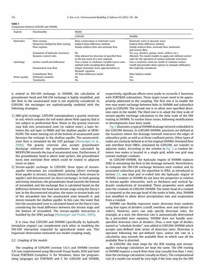
Table 1Comparison between GSFLOW and SWMM.

Aspects Functionality Model

GSFLOW SWMM

Hydraulics Flow routing Mass conservation or kinematic wave Kinematic wave or dynamic waveNumerical method for flow routing Implicit finite difference method Explicit finite difference methodFlow regimes Steady-uniform flow and unsteady flow Steady-uniform flow, unsteady flow, backwater

and reverse flowSimulation of hydraulic structures No Yes (e.g., dividers, pumps, weirs, orifices, etc.)Dynamic control rules Only allowed for diversion of specified flow

at the last reach of a river segmentAllowed. The model enables to apply user-defined controlrules for the operation of various hydraulic structures

Hydrology Surface runoff and Infiltration Uses a linear or nonlinear variable-source-areamethod with cascading flow allowed

Uses a nonlinear reservoir model to simulate surfacerunoff and provides three options to simulate infiltration

Unsaturated-zone flow Adopts kinematic-wave approximation toRichards' equation

Not explicitly considered

Groundwater flow 3D finite-difference model Mass balance modelWater quality Pollutants modeled No Yes

Treatments No Yes

Y. Tian et al. / Environmental Modelling & Software 63 (2015) 170e184172

is related to SW-GW exchange. In SWMM, the calculation ofgroundwater head and SW-GW exchange is highly simplified, andthe flow in the unsaturated zone is not explicitly considered. InGSFLOW, the exchanges are sophisticatedly modeled with thefollowing strategies.

1) HRU-grid exchange. GSFLOW conceptualizes a gravity reservoirin soil, which contains the soil water above field capacity that isnot subject to preferential flow. Water in the gravity reservoirmay leak into unsaturated zone (or vadose zone), a layer be-tween the soil layer in PRMS and the shallow aquifer in MOD-FLOW. The water moving out of the bottom of unsaturated zonebecomes the recharge to the shallow aquifer. The unsaturated-zone flow is simulated by the UZF package (Niswonger et al.,2006). The gravity reservoir also accepts groundwaterdischarge whenever the groundwater head calculated byMODFLOWexceeds the top of unsaturated zone. Furthermore, ifthe groundwater head is above land surface, the groundwaterturns into overland flow which could be routed to adjacentrivers or lakes.

2) Stream-aquifer exchange. In GSFLOW, three types of stream-aquifer interaction are considered: gaining (direct exchangefrom aquifer to stream), losing (direct exchange from stream toaquifer) and disconnected (no direct exchange). In both gainingand losing situations, the groundwater head exceeds the bottomof streambed, and the exchange flux is calculated based on thedifference between the head and stream stage using the Darcy'slaw. In the disconnected situation, the water in stream leaks outof the streambed into the unsaturated zone beneath it, andmoves towards the shallow aquifer. In this case, the water fluxinto the unsaturated zone is calculated based on the Darcy's law,considering the head difference between the stream stage andthe bottom of streambed. The stream-aquifer interaction ishandled by the SFR2 package (Niswonger and Prudic, 2005).

It is clear that GSFLOW and SWMM (specifically its hydraulicsimulation engine) can complement each other in modeling theSW-GW interaction impacted by agricultural water use. Thisimportant observation motivated our model coupling study.

2.2. Coupling of the models

The coupling of GSFLOW (version 1.6.1) and SWMM (version5.0) was implemented using Microsoft Visual Studio 2010 and IntelVisual FORTRAN Compilers 11 for Windows. Since the program-ming languages are FORTRAN and C for GSFLOW and SWMM,

respectively, significant efforts were made to reconcile C functionswith FORTRAN subroutines. Three major issues need to be appro-priately addressed in the coupling. The first one is to enable thetwo-way water exchange between links in SWMM and subsurfacegrids in GSFLOW. The second one is to allow user-specified diver-sion rates in the model. The third one is to adapt the time scale ofstream-aquifer exchange calculation to the time scale of the DWrouting in SWMM. To resolve these issues, following modificationsor developments have been made.

Fig.1 illustrates a typical SWMMdrainage network embedded inthe GSFLOW domain. In GSFLOW-SWMM, junctions are defined atthe locations where the drainage network intersects the edges ofsubsurface grids, as well as at those confluent points. Other types ofnodes are similarly defined as in the original SWMM. Overland flowand interflow from HRUs, simulated by GSFLOW, are transfer toadjacent nodes. According to the scheme in Fig. 1, a conduit be-tween two nodes is located in a single grid, while one grid maycontain multiple conduits.

In GSFLOW-SWMM, the hydraulic engine of SWMM replacesSFR2 in simulating the flow in the drainage network. Nevertheless,to compute the SW-GW exchange between each conduit and itsassociated subsurface grid, the algorithm in SFR2, as introduced inSection 2.1, was kept and re-coded into the hydraulic engine ofSWMM. Conduits in SWMM do not have the properties in relationto stream-aquifer interaction, such as thickness and vertical hy-draulic conductivity of streambed. These properties were addedonto the conduits in GSFLOW-SWMM. The water head of a conduitis computed as the average head of the nodes it links. Also, SWMMwas modified to allow direct precipitation into and evaporationfrom a conduit.

SWMM can flexibly represent water diversion from conduitsusing four types of dividers (cutoff, overflow, weir and tabular di-viders). However, users can only specify diversion rules. Forexample, at a weir, the diversion rate is automatically determinedby a prescribed weir equation. SWMM does not handle user-specified diversion rates at dividers. Thus, a new type of divider,named as “schedule divider”, was added in GSFLOW-SWMMwhichaccepts user-defined time series of diversion rates. Diversion isoperated following the pre-defined rates, unless the rate in acalculation step exceeds the available flow, in which case all theavailable flow is diverted.

In GSFLOW, the time steps for the KW routing and stream-aquifer exchange calculation are kept the same. The DW routingin SWMM requires a much finer time step (usually less than 1 min)than the exchange calculation (usually an hour). The computationalcost of a model run would be very high if the time step for the DW

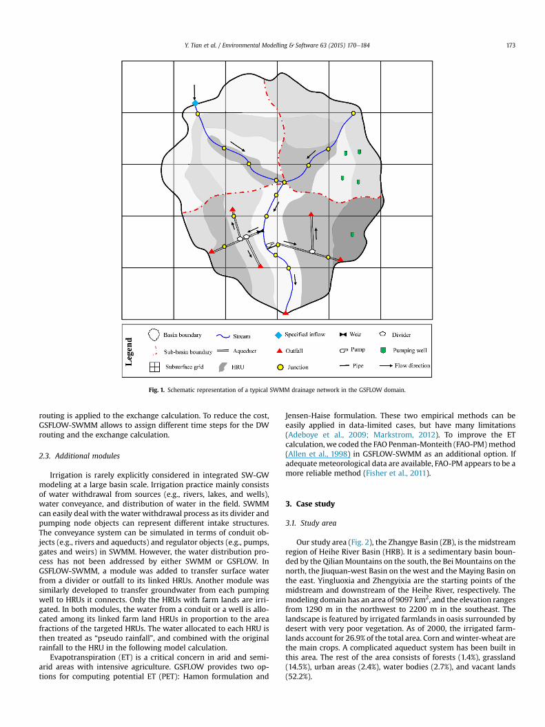
Fig. 1. Schematic representation of a typical SWMM drainage network in the GSFLOW domain.

Y. Tian et al. / Environmental Modelling & Software 63 (2015) 170e184 173

routing is applied to the exchange calculation. To reduce the cost,GSFLOW-SWMM allows to assign different time steps for the DWrouting and the exchange calculation.

2.3. Additional modules

Irrigation is rarely explicitly considered in integrated SW-GWmodeling at a large basin scale. Irrigation practice mainly consistsof water withdrawal from sources (e.g., rivers, lakes, and wells),water conveyance, and distribution of water in the field. SWMMcan easily deal with the water withdrawal process as its divider andpumping node objects can represent different intake structures.The conveyance system can be simulated in terms of conduit ob-jects (e.g., rivers and aqueducts) and regulator objects (e.g., pumps,gates and weirs) in SWMM. However, the water distribution pro-cess has not been addressed by either SWMM or GSFLOW. InGSFLOW-SWMM, a module was added to transfer surface waterfrom a divider or outfall to its linked HRUs. Another module wassimilarly developed to transfer groundwater from each pumpingwell to HRUs it connects. Only the HRUs with farm lands are irri-gated. In both modules, the water from a conduit or a well is allo-cated among its linked farm land HRUs in proportion to the areafractions of the targeted HRUs. The water allocated to each HRU isthen treated as “pseudo rainfall”, and combined with the originalrainfall to the HRU in the following model calculation.

Evapotranspiration (ET) is a critical concern in arid and semi-arid areas with intensive agriculture. GSFLOW provides two op-tions for computing potential ET (PET): Hamon formulation and

Jensen-Haise formulation. These two empirical methods can beeasily applied in data-limited cases, but have many limitations(Adeboye et al., 2009; Markstrom, 2012). To improve the ETcalculation, we coded the FAO Penman-Monteith (FAO-PM)method(Allen et al., 1998) in GSFLOW-SWMM as an additional option. Ifadequatemeteorological data are available, FAO-PM appears to be amore reliable method (Fisher et al., 2011).

3. Case study

3.1. Study area

Our study area (Fig. 2), the Zhangye Basin (ZB), is the midstreamregion of Heihe River Basin (HRB). It is a sedimentary basin boun-ded by the QilianMountains on the south, the Bei Mountains on thenorth, the Jiuquan-west Basin on the west and the Maying Basin onthe east. Yingluoxia and Zhengyixia are the starting points of themidstream and downstream of the Heihe River, respectively. Themodeling domain has an area of 9097 km2, and the elevation rangesfrom 1290 m in the northwest to 2200 m in the southeast. Thelandscape is featured by irrigated farmlands in oasis surrounded bydesert with very poor vegetation. As of 2000, the irrigated farm-lands account for 26.9% of the total area. Corn andwinter-wheat arethe main crops. A complicated aqueduct system has been built inthis area. The rest of the area consists of forests (1.4%), grassland(14.5%), urban areas (2.4%), water bodies (2.7%), and vacant lands(52.2%).

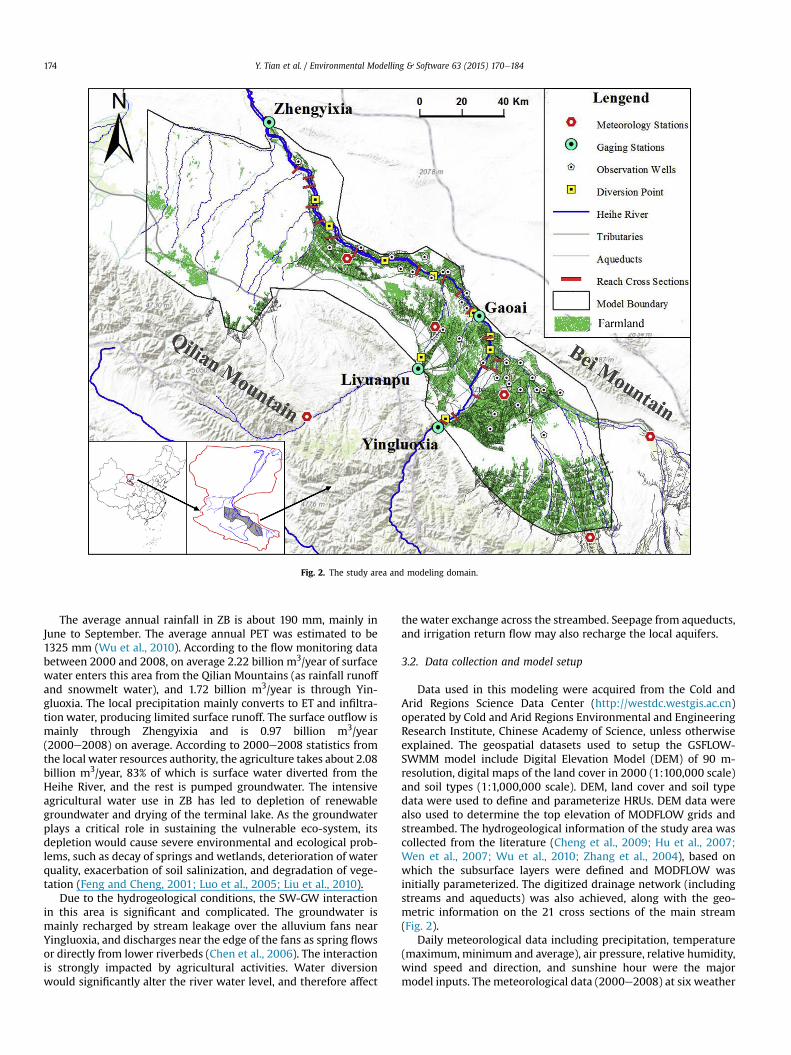
Fig. 2. The study area and modeling domain.

Y. Tian et al. / Environmental Modelling & Software 63 (2015) 170e184174

The average annual rainfall in ZB is about 190 mm, mainly inJune to September. The average annual PET was estimated to be1325 mm (Wu et al., 2010). According to the flow monitoring databetween 2000 and 2008, on average 2.22 billion m3/year of surfacewater enters this area from the Qilian Mountains (as rainfall runoffand snowmelt water), and 1.72 billion m3/year is through Yin-gluoxia. The local precipitation mainly converts to ET and infiltra-tion water, producing limited surface runoff. The surface outflow ismainly through Zhengyixia and is 0.97 billion m3/year(2000e2008) on average. According to 2000e2008 statistics fromthe local water resources authority, the agriculture takes about 2.08billion m3/year, 83% of which is surface water diverted from theHeihe River, and the rest is pumped groundwater. The intensiveagricultural water use in ZB has led to depletion of renewablegroundwater and drying of the terminal lake. As the groundwaterplays a critical role in sustaining the vulnerable eco-system, itsdepletion would cause severe environmental and ecological prob-lems, such as decay of springs and wetlands, deterioration of waterquality, exacerbation of soil salinization, and degradation of vege-tation (Feng and Cheng, 2001; Luo et al., 2005; Liu et al., 2010).

Due to the hydrogeological conditions, the SW-GW interactionin this area is significant and complicated. The groundwater ismainly recharged by stream leakage over the alluvium fans nearYingluoxia, and discharges near the edge of the fans as spring flowsor directly from lower riverbeds (Chen et al., 2006). The interactionis strongly impacted by agricultural activities. Water diversionwould significantly alter the river water level, and therefore affect

the water exchange across the streambed. Seepage from aqueducts,and irrigation return flow may also recharge the local aquifers.

3.2. Data collection and model setup

Data used in this modeling were acquired from the Cold andArid Regions Science Data Center (http://westdc.westgis.ac.cn)operated by Cold and Arid Regions Environmental and EngineeringResearch Institute, Chinese Academy of Science, unless otherwiseexplained. The geospatial datasets used to setup the GSFLOW-SWMM model include Digital Elevation Model (DEM) of 90 m-resolution, digital maps of the land cover in 2000 (1:100,000 scale)and soil types (1:1,000,000 scale). DEM, land cover and soil typedata were used to define and parameterize HRUs. DEM data werealso used to determine the top elevation of MODFLOW grids andstreambed. The hydrogeological information of the study area wascollected from the literature (Cheng et al., 2009; Hu et al., 2007;Wen et al., 2007; Wu et al., 2010; Zhang et al., 2004), based onwhich the subsurface layers were defined and MODFLOW wasinitially parameterized. The digitized drainage network (includingstreams and aqueducts) was also achieved, along with the geo-metric information on the 21 cross sections of the main stream(Fig. 2).

Daily meteorological data including precipitation, temperature(maximum, minimum and average), air pressure, relative humidity,wind speed and direction, and sunshine hour were the majormodel inputs. The meteorological data (2000e2008) at six weather

Y. Tian et al. / Environmental Modelling & Software 63 (2015) 170e184 175

stations (see Fig. 2) were collected and extrapolated to each HRUusing the Gradient plus Inverse Distance Weighting (GIDW)method (Nalder and Wein, 1998).

River diversion and groundwater pumping data are alsoimportant model inputs. The monthly diversion and yearlypumping data of the 20 irrigation districts in this area werecollected from the local water resources authority of the ZhangyeCity. For some of the districts, we only obtained yearly diversiondata, and their monthly estimates were determined on the basis ofintra-month allocation pattern observed from other districts. Inorder to improve simulations of daily streamflow, daily diversiondatawere estimated by downscaling themonthly data based on ourinvestigation on the local agricultural practice and analysis on theobserved hydrographs of the Heihe River. For each individual dis-trict, the daily estimates may not be accurate, but for the study areaas a whole they reflect well the intra-month variation of thediversion. Pumping was taken into account with the Well moduleof GSFLOW. As we only have yearly pumping data by districts, aconstant pumping rate was applied uniformly in each district ineach year. The rate only varies across years and across districts.

The modeling domain is similar to that in Hu et al. (2007).Thesouth and north subsurface boundaries used specific flow condi-tions, receiving groundwater flow from the Qilian Mountains andthe Bei Mountains, respectively. The boundary flow fluxes wereinitially estimated based on the observed hydraulic gradient of thegroundwater and the hydraulic conductivity near the boundary(Wu et al., 2010). No-flow conditions were applied to the west andeast subsurface boundaries, since there exist groundwater divides(Hu et al., 2007). The daily flow rates at the Yingluoxia andLiyuanpu stations were used as surface water boundary conditions.

The surface domain was delineated into 104 sub-basins and 588HRUs. The subsurface was divided into five layers, each with 9106active cells (1 km� 1 km). The first layer represents an unconfinedaquifer, the second and fourth layers represent aquitards, and thethird and fifth layers represent confined aquifers. From the top tothe bottom, the five layers were respectively divided into 21, 12, 14,12, and 14 zones for model parameterization. The drainage networkin themodel is comprised of 1697 junctions,18 outfalls, 12 scheduledividers (i.e., the 12 diversion points shown in Fig. 2) and 1594conduits (i.e., river and aqueduct elements). As we only have thecross-section details for themain stream, rectangular cross sectionswere assumed for conduits not in the main stream. The streambedhydraulic conductivity and Manning's roughness coefficient wereestimated based on field surveys and the hydrogeological infor-mation we collected. With all the necessary data collected, themodel was setup with external tools including ArcGIS andModelMuse.

Note that, besides streamflow and groundwater level, GSFLOWoutputs a number of state variables (e.g., soil moisture, canopystorage, stream storage, saturated zone storage, etc.) and fluxes(e.g., ET, surface water infiltration, groundwater exfiltration, streamleakage, interflow, etc.). Thus, a detailed regional water budget, aswell as the flux between the budget items, can be readily achievedwith the model simulation. Conceptually, for the study area, themajor water inputs, with descending importance, are upstreamsurface inflow, local precipitation and lateral groundwater inflowfrom the south (Qilian Mountains) and north (Bei Mountains)boundaries. The major water outputs are ET and surface wateroutflow (mostly through Zhengyixia), and no lateral groundwateroutflow has been assumed. Internal water exchanges mainlyinclude surface water recharge to unsaturated zone and saturatedzone, and groundwater discharge to land surface and stream.Nevertheless, a coherent and quantitative understanding of theregional water budget is yet to be developed. This study applied thecoupled GSFLOW-SWMM model to achieve this.

3.3. Model calibration

Daily streamflow observations (2000e2008) were obtained atfour gaging stations (Fig. 2). Observations at the Yingluoxia andLiyuanpu stations were used to set the surface water boundaryconditions, and observations at the Gaoai and Zhengyixia stationswere used for the model calibration. Monthly groundwater levelmeasurements (2000e2004) at 35 observation wells (see Fig. 2)were obtained and used for the calibration as well.

To set the initial condition for transient simulations, a steady-state MODFLOW simulation was first performed, which is a com-mon practice in applying MODFLOW. Key groundwater parameters(i.e., hydraulic conductivities) were adjusted in this stage. In thenext stage, the GSFLLOW-SWMM model was run at a daily time-step for a nine-year period from 01/01/2000 to 12/31/2008 (thetime-step for the SW-GWexchange calculation is hourly). To have areasonable initial storage of the soil zone (Huntington andNiswonger, 2012), the first year was treated as a “spin-up’’ periodand therefore excluded from the calibration. Key model parametersfor both surface water and groundwater were further tuned toreproduce the observed temporal variability of streamflow andgroundwater level. Additional information was referred to furtherconstrain the model calibration, including the ET informationdrawn from remote sensing data (Li et al., 2012), the regional SW-GWexchange and groundwater storage change estimated by waterbalance calculation (Cheng et al., 2009), as well as river bed leakageestimated from field measurements and isotope experiments (Wuet al., 2010).

The calibration was manually accomplished in a trial-and-errormanner. For groundwater level, after the hydraulic conductivitieswere adjusted through steady-state simulations, specific yieldswere further tuned through transient simulations. As we do nothave temporally and spatially detailed information on the localpumping which would significantly alter the groundwater level,the calibration was aimed to capture the long-term characteristicsof the regional groundwater level, rather than to precisely repro-duce the dynamics of groundwater level in individual wells. Forstreamflow, besides the classic Nash-Sutcliffe model efficiency(NSE) (Nash and Sutcliffe, 1970), two additional goodness-of-fitmeasures, logNSE and percentage bias (BIAS), were considered.Compared to NSE, logNSE is less sensitive to peak flow. BIAS mea-sures whether the flow is systematically overestimated (positiveBIAS) or underestimated (negative BIAS). A limited number of pa-rameters were found to be critical to streamflow calibration. Themajor adjusted ones include soil's maximum available capillarywater-holding capacity, maximumdepth where evapotranspirationcan occur and maximum possible area contributing to surfacerunoff in PRMS, and hydraulic conductivity of streambed in themodified hydraulic engine of SWMM. Note that specific yield andhorizontal hydraulic conductivity were also found to be importantto the streamflow calibration, but they were mainly tuned in thegroundwater calibration.

In addition, our preliminary tests showed that using the dy-namic wave (DW) method for flow routing (with a time-step of30 s) instead of the kinematic wave (KW) method made no sig-nificant differences in this modeling case. Therefore, the KWmethod was used throughout this study to save the computationalcost.

3.4. Sensitivity analysis

To further explore how major model outputs respond to majorinput variables, a simple one-factor-at-a-time (OAT) sensitivityanalysis (SA) was performed. Thirteen model outputs wereconsidered, including ET, soil moisture (SM), infiltration (IFL), UZF

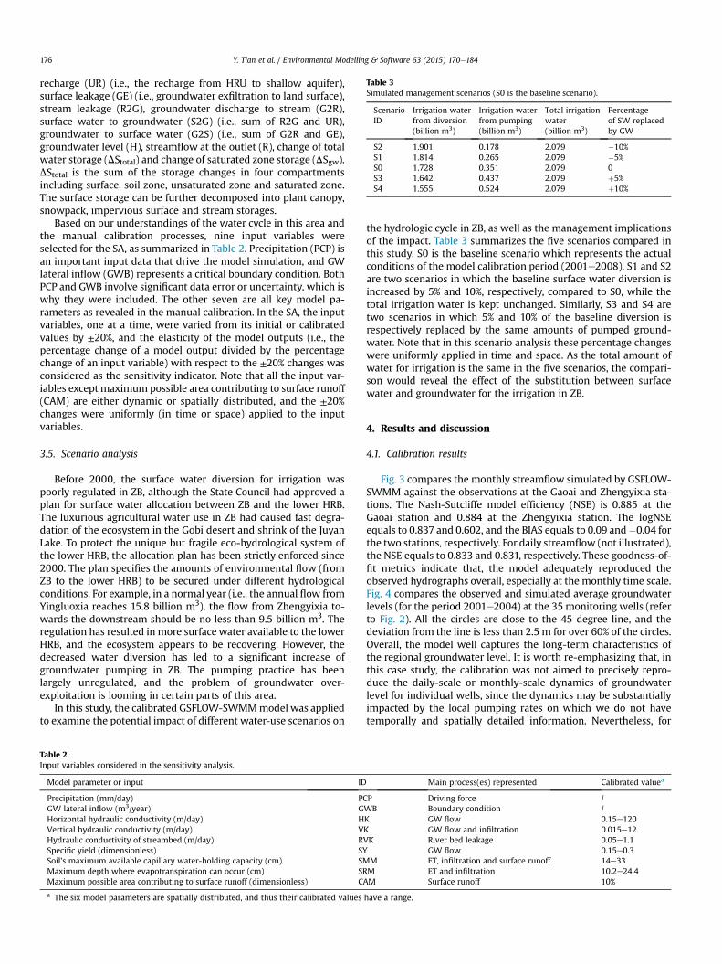
Table 3Simulated management scenarios (S0 is the baseline scenario).

ScenarioID

Irrigation waterfrom diversion(billion m3)

Irrigation waterfrom pumping(billion m3)

Total irrigationwater(billion m3)

Percentageof SW replacedby GW

S2 1.901 0.178 2.079 �10%S1 1.814 0.265 2.079 �5%S0 1.728 0.351 2.079 0S3 1.642 0.437 2.079 þ5%S4 1.555 0.524 2.079 þ10%

Y. Tian et al. / Environmental Modelling & Software 63 (2015) 170e184176

recharge (UR) (i.e., the recharge from HRU to shallow aquifer),surface leakage (GE) (i.e., groundwater exfiltration to land surface),stream leakage (R2G), groundwater discharge to stream (G2R),surface water to groundwater (S2G) (i.e., sum of R2G and UR),groundwater to surface water (G2S) (i.e., sum of G2R and GE),groundwater level (H), streamflow at the outlet (R), change of totalwater storage (DStotal) and change of saturated zone storage (DSgw).DStotal is the sum of the storage changes in four compartmentsincluding surface, soil zone, unsaturated zone and saturated zone.The surface storage can be further decomposed into plant canopy,snowpack, impervious surface and stream storages.

Based on our understandings of the water cycle in this area andthe manual calibration processes, nine input variables wereselected for the SA, as summarized in Table 2. Precipitation (PCP) isan important input data that drive the model simulation, and GWlateral inflow (GWB) represents a critical boundary condition. BothPCP and GWB involve significant data error or uncertainty, which iswhy they were included. The other seven are all key model pa-rameters as revealed in the manual calibration. In the SA, the inputvariables, one at a time, were varied from its initial or calibratedvalues by ±20%, and the elasticity of the model outputs (i.e., thepercentage change of a model output divided by the percentagechange of an input variable) with respect to the ±20% changes wasconsidered as the sensitivity indicator. Note that all the input var-iables except maximum possible area contributing to surface runoff(CAM) are either dynamic or spatially distributed, and the ±20%changes were uniformly (in time or space) applied to the inputvariables.

3.5. Scenario analysis

Before 2000, the surface water diversion for irrigation waspoorly regulated in ZB, although the State Council had approved aplan for surface water allocation between ZB and the lower HRB.The luxurious agricultural water use in ZB had caused fast degra-dation of the ecosystem in the Gobi desert and shrink of the JuyanLake. To protect the unique but fragile eco-hydrological system ofthe lower HRB, the allocation plan has been strictly enforced since2000. The plan specifies the amounts of environmental flow (fromZB to the lower HRB) to be secured under different hydrologicalconditions. For example, in a normal year (i.e., the annual flow fromYingluoxia reaches 15.8 billion m3), the flow from Zhengyixia to-wards the downstream should be no less than 9.5 billion m3. Theregulation has resulted in more surface water available to the lowerHRB, and the ecosystem appears to be recovering. However, thedecreased water diversion has led to a significant increase ofgroundwater pumping in ZB. The pumping practice has beenlargely unregulated, and the problem of groundwater over-exploitation is looming in certain parts of this area.

In this study, the calibrated GSFLOW-SWMMmodel was appliedto examine the potential impact of different water-use scenarios on

Table 2Input variables considered in the sensitivity analysis.

Model parameter or input ID

Precipitation (mm/day) PCGW lateral inflow (m3/year) GHorizontal hydraulic conductivity (m/day) HVertical hydraulic conductivity (m/day) VHydraulic conductivity of streambed (m/day) RSpecific yield (dimensionless) SYSoil's maximum available capillary water-holding capacity (cm) SMMaximum depth where evapotranspiration can occur (cm) SRMaximum possible area contributing to surface runoff (dimensionless) C

a The six model parameters are spatially distributed, and thus their calibrated values

the hydrologic cycle in ZB, as well as the management implicationsof the impact. Table 3 summarizes the five scenarios compared inthis study. S0 is the baseline scenario which represents the actualconditions of the model calibration period (2001e2008). S1 and S2are two scenarios in which the baseline surface water diversion isincreased by 5% and 10%, respectively, compared to S0, while thetotal irrigation water is kept unchanged. Similarly, S3 and S4 aretwo scenarios in which 5% and 10% of the baseline diversion isrespectively replaced by the same amounts of pumped ground-water. Note that in this scenario analysis these percentage changeswere uniformly applied in time and space. As the total amount ofwater for irrigation is the same in the five scenarios, the compari-son would reveal the effect of the substitution between surfacewater and groundwater for the irrigation in ZB.

4. Results and discussion

4.1. Calibration results

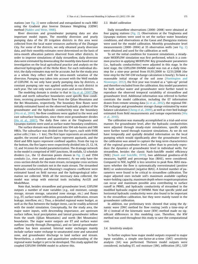
Fig. 3 compares the monthly streamflow simulated by GSFLOW-SWMM against the observations at the Gaoai and Zhengyixia sta-tions. The Nash-Sutcliffe model efficiency (NSE) is 0.885 at theGaoai station and 0.884 at the Zhengyixia station. The logNSEequals to 0.837 and 0.602, and the BIAS equals to 0.09 and�0.04 forthe two stations, respectively. For daily streamflow (not illustrated),the NSE equals to 0.833 and 0.831, respectively. These goodness-of-fit metrics indicate that, the model adequately reproduced theobserved hydrographs overall, especially at the monthly time scale.Fig. 4 compares the observed and simulated average groundwaterlevels (for the period 2001e2004) at the 35 monitoring wells (referto Fig. 2). All the circles are close to the 45-degree line, and thedeviation from the line is less than 2.5 m for over 60% of the circles.Overall, the model well captures the long-term characteristics ofthe regional groundwater level. It is worth re-emphasizing that, inthis case study, the calibration was not aimed to precisely repro-duce the daily-scale or monthly-scale dynamics of groundwaterlevel for individual wells, since the dynamics may be substantiallyimpacted by the local pumping rates on which we do not havetemporally and spatially detailed information. Nevertheless, for

Main process(es) represented Calibrated valuea

P Driving force /WB Boundary condition /K GW flow 0.15e120K GW flow and infiltration 0.015e12VK River bed leakage 0.05e1.1

GW flow 0.15e0.3M ET, infiltration and surface runoff 14e33M ET and infiltration 10.2e24.4

AM Surface runoff 10%

have a range.

Fig. 3. Comparison of simulated and observed monthly streamflow at (a) the Gaoai station; and (b) the Zhengyixia station.

Y. Tian et al. / Environmental Modelling & Software 63 (2015) 170e184 177

many wells, the calibrated model can still capture the main tem-poral trend, as demonstrated by Fig. 5. The five selected wells arelocated in places where the groundwater fluctuation is controlledby the SW-GW interaction and less impacted by the pumping.

Fig. 4. Comparison of the observed and simulated groundwater levels averaged for theperiod 2001e2004. Each circle represents one of the 35 observation wells.

Some problems with the calibration were also observed, whichcould be mainly due to data imperfections. First, the logNSE at theZhengyixia station is relatively small, because the near-zero flowduring April to June was not well simulated (Fig. 3). Since the flowat the upstream Gaoai station during the same period was signifi-cant and the Heihe River between Gaoai and Zhengyixia is not alosing segment, the near-zero flow has to be caused by the sub-stantial water diversion for irrigation in this segment. It thereforesuggests that the diversion data we collected and input into themodel may underestimate the actual amount during that period.Second, the positive BIAS (i.e., 0.09) at the Gaoai station is relativelyhigh, mainly because the peak flow was overestimated in most ofthe years (Fig. 3). It is known that the local precipitation contributesa limited amount of water to the streamflow at Gaoai, and the peakflow at that point largely reflects the peak flow out of Yingluoxia(around 65 km upstream of Gaoai) which has been well gaged. Onthe other hand, the stream leakage in the segment between Yin-gluoxia and Gaoai has already been tuned to an appropriate level,referring to field measurements and isotope experiments (Wuet al., 2010). Thus, the systematic overestimation is most likelycaused by the inaccurate (underestimated) diversion data of thissegment. Third, the smaller NSE values for the daily streamflowsimulation may be due to the inaccuracy of daily diversion esti-mates that were downscaled from the monthly diversion data.

As discussed in Bennett et al. (2013), a number of metrics, be-sides NSE, logNSE and BIAS, could be considered to quantitativelyevaluate the model performance, and the calibration procedure inthis study is not a rigorousmethod for the evaluation. Nevertheless,

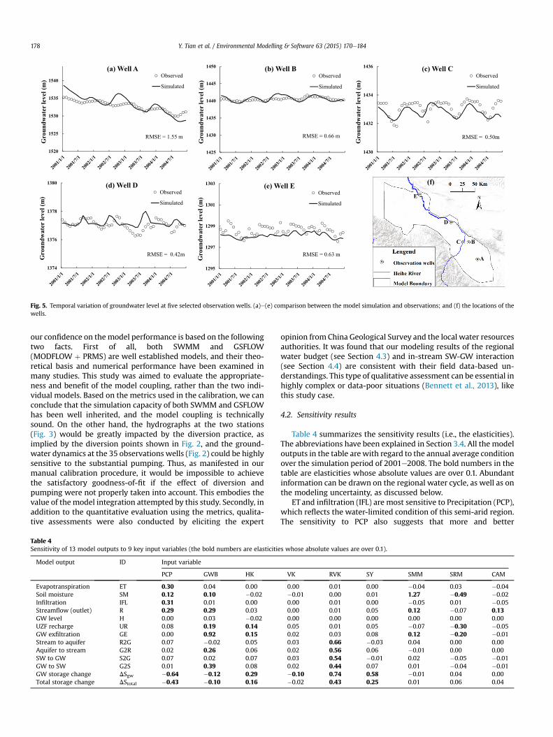
Fig. 5. Temporal variation of groundwater level at five selected observation wells. (a)e(e) comparison between the model simulation and observations; and (f) the locations of thewells.

Y. Tian et al. / Environmental Modelling & Software 63 (2015) 170e184178

our confidence on themodel performance is based on the followingtwo facts. First of all, both SWMM and GSFLOW(MODFLOW þ PRMS) are well established models, and their theo-retical basis and numerical performance have been examined inmany studies. This study was aimed to evaluate the appropriate-ness and benefit of the model coupling, rather than the two indi-vidual models. Based on the metrics used in the calibration, we canconclude that the simulation capacity of both SWMM and GSFLOWhas been well inherited, and the model coupling is technicallysound. On the other hand, the hydrographs at the two stations(Fig. 3) would be greatly impacted by the diversion practice, asimplied by the diversion points shown in Fig. 2, and the ground-water dynamics at the 35 observations wells (Fig. 2) could be highlysensitive to the substantial pumping. Thus, as manifested in ourmanual calibration procedure, it would be impossible to achievethe satisfactory goodness-of-fit if the effect of diversion andpumping were not properly taken into account. This embodies thevalue of the model integration attempted by this study. Secondly, inaddition to the quantitative evaluation using the metrics, qualita-tive assessments were also conducted by eliciting the expert

Table 4Sensitivity of 13 model outputs to 9 key input variables (the bold numbers are elasticitie

Model output ID Input variable

PCP GWB HK

Evapotranspiration ET 0.30 0.04 0.00Soil moisture SM 0.12 0.10 �0.02Infiltration IFL 0.31 0.01 0.00Streamflow (outlet) R 0.29 0.29 0.03GW level H 0.00 0.03 �0.02UZF recharge UR 0.08 0.19 0.14GW exfiltration GE 0.00 0.92 0.15Stream to aquifer R2G 0.07 �0.02 0.05Aquifer to stream G2R 0.02 0.26 0.06SW to GW S2G 0.07 0.02 0.07GW to SW G2S 0.01 0.39 0.08GW storage change DSgw �0.64 �0.12 0.29Total storage change DStotal �0.43 �0.10 0.16

opinion from China Geological Survey and the local water resourcesauthorities. It was found that our modeling results of the regionalwater budget (see Section 4.3) and in-stream SW-GW interaction(see Section 4.4) are consistent with their field data-based un-derstandings. This type of qualitative assessment can be essential inhighly complex or data-poor situations (Bennett et al., 2013), likethis study case.

4.2. Sensitivity results

Table 4 summarizes the sensitivity results (i.e., the elasticities).The abbreviations have been explained in Section 3.4. All the modeloutputs in the table are with regard to the annual average conditionover the simulation period of 2001e2008. The bold numbers in thetable are elasticities whose absolute values are over 0.1. Abundantinformation can be drawn on the regional water cycle, as well as onthe modeling uncertainty, as discussed below.

ET and infiltration (IFL) are most sensitive to Precipitation (PCP),which reflects the water-limited condition of this semi-arid region.The sensitivity to PCP also suggests that more and better

s whose absolute values are over 0.1).

VK RVK SY SMM SRM CAM

0.00 0.01 0.00 �0.04 0.03 �0.04�0.01 0.00 0.01 1.27 �0.49 �0.020.00 0.01 0.00 �0.05 0.01 �0.050.00 0.01 0.05 0.12 �0.07 0.130.00 0.00 0.00 0.00 0.00 0.000.05 0.01 0.05 �0.07 �0.30 �0.050.02 0.03 0.08 0.12 �0.20 �0.010.03 0.66 �0.03 0.04 0.00 0.000.02 0.56 0.06 �0.01 0.00 0.000.03 0.54 �0.01 0.02 �0.05 �0.010.02 0.44 0.07 0.01 �0.04 �0.01�0.10 0.74 0.58 �0.01 0.04 0.00�0.02 0.43 0.25 0.01 0.06 0.04

Y. Tian et al. / Environmental Modelling & Software 63 (2015) 170e184 179

precipitation data are desired to improve the estimation of ET andIFL, since only six meteorological stations (see Fig. 2) are currentlyavailable for interpolating the distribution of precipitation.

For those SW-GW exchange fluxes (i.e., from UR to G2S inTable 4), GW lateral inflow (GWB) and hydraulic conductivity ofstreambed (RVK) appear to be the most influential factors, whichindicates that the GW-SW exchange mostly occurs in the river andlargely depends on the subsurface boundary inflow from the up-stream. As GWB and RVK are highly uncertain input and parameter,respectively, in the modeling, hydrogeological surveys are desiredto achieve more accurate data for reducing the modelinguncertainty.

Soil moisture (SM) is most sensitive to the two soil parameterssoil's maximum available capillary water-holding capacity (SMM)and maximum depth where ET can occur (SRM). As PCP and GWBrepresent two important water inputs to the system, they also havea notable impact on SM. For streamflow at the outlet (R), besidesPCP and GWB, SMM and maximum possible area contributing tosurface runoff (CAM) were found to be important as well. Thesesensitivity results were well expected, given the hydrologicalmeanings of the input variables (refer to Table 2). GW level (H),however, appears to be insensitive to all the input variables. This isnot because H does not respond to them, but because the elasticityis not an appropriate sensitivity measure for H. H is defined basedon elevationwhich is above 1000 m in this area. Thus, the variationof H (usually several meters) is order of magnitude lower than theelevation, which results in the small elasticity values.

On the other hand, the impact of the input variables on thegroundwater system is well demonstrated by the sensitivity of GWstorage change (DSgw). Besides PCP, GWB and RVK, horizontal hy-draulic conductivity (HK) and specific yield (SY) are two additionalinfluential parameters for DSgw, since they determine how fast andhow much water could be released from the aquifer. Total storagechange (DStotal) exhibits a similar sensitivity pattern as DSgw, whichreflects the modeling result that DSgw is a major component ofDStotal (see Section 4.3 for more details).

Overall, the sensitivity analysis demonstrated that the inte-grated modeling is valuable for understanding the water cycle in alarge basin with complicated SW-GW interaction.

4.3. Regional water budget

Figs. 3e5 suggest that the GSFLOW-SWMM model has beenadequately calibrated to simulate the general behavior of the SW-GW system in ZB. The simulated annual water budget (averaged

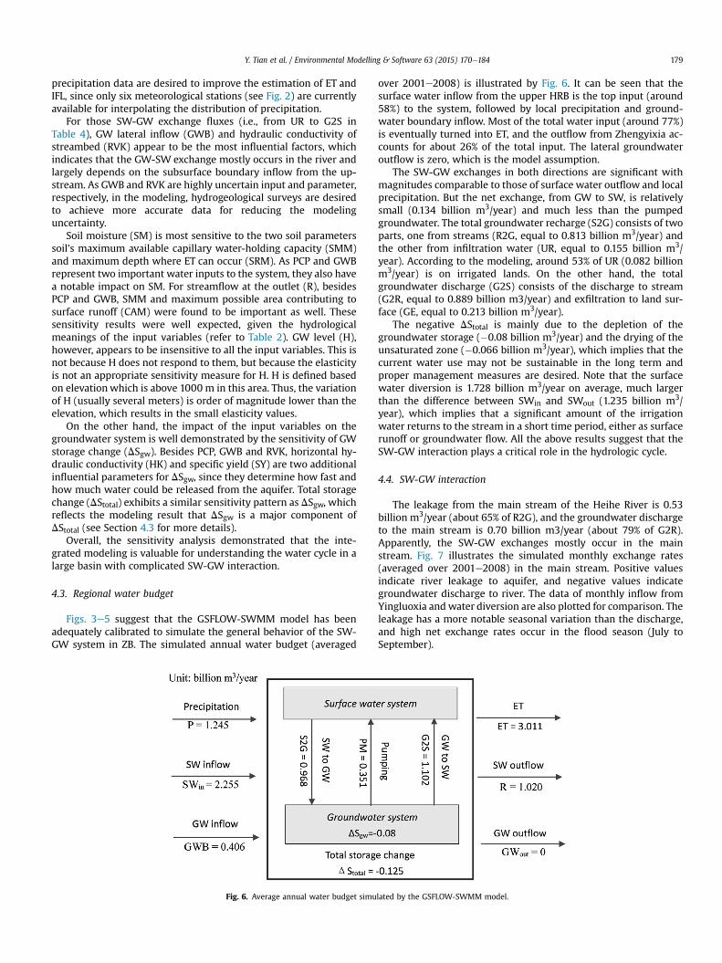
Fig. 6. Average annual water budget simu

over 2001e2008) is illustrated by Fig. 6. It can be seen that thesurface water inflow from the upper HRB is the top input (around58%) to the system, followed by local precipitation and ground-water boundary inflow. Most of the total water input (around 77%)is eventually turned into ET, and the outflow from Zhengyixia ac-counts for about 26% of the total input. The lateral groundwateroutflow is zero, which is the model assumption.

The SW-GW exchanges in both directions are significant withmagnitudes comparable to those of surface water outflow and localprecipitation. But the net exchange, from GW to SW, is relativelysmall (0.134 billion m3/year) and much less than the pumpedgroundwater. The total groundwater recharge (S2G) consists of twoparts, one from streams (R2G, equal to 0.813 billion m3/year) andthe other from infiltration water (UR, equal to 0.155 billion m3/year). According to the modeling, around 53% of UR (0.082 billionm3/year) is on irrigated lands. On the other hand, the totalgroundwater discharge (G2S) consists of the discharge to stream(G2R, equal to 0.889 billion m3/year) and exfiltration to land sur-face (GE, equal to 0.213 billion m3/year).

The negative DStotal is mainly due to the depletion of thegroundwater storage (�0.08 billion m3/year) and the drying of theunsaturated zone (�0.066 billion m3/year), which implies that thecurrent water use may not be sustainable in the long term andproper management measures are desired. Note that the surfacewater diversion is 1.728 billion m3/year on average, much largerthan the difference between SWin and SWout (1.235 billion m3/year), which implies that a significant amount of the irrigationwater returns to the stream in a short time period, either as surfacerunoff or groundwater flow. All the above results suggest that theSW-GW interaction plays a critical role in the hydrologic cycle.

4.4. SW-GW interaction

The leakage from the main stream of the Heihe River is 0.53billion m3/year (about 65% of R2G), and the groundwater dischargeto the main stream is 0.70 billion m3/year (about 79% of G2R).Apparently, the SW-GW exchanges mostly occur in the mainstream. Fig. 7 illustrates the simulated monthly exchange rates(averaged over 2001e2008) in the main stream. Positive valuesindicate river leakage to aquifer, and negative values indicategroundwater discharge to river. The data of monthly inflow fromYingluoxia and water diversion are also plotted for comparison. Theleakage has a more notable seasonal variation than the discharge,and high net exchange rates occur in the flood season (July toSeptember).

lated by the GSFLOW-SWMM model.

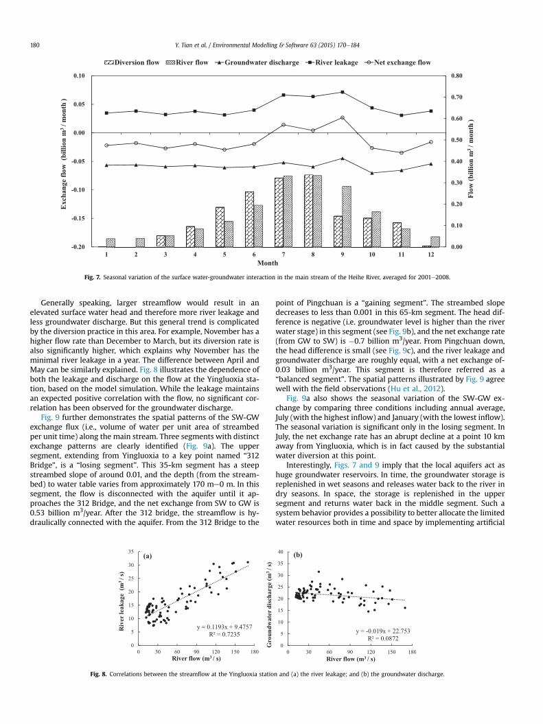
Fig. 7. Seasonal variation of the surface water-groundwater interaction in the main stream of the Heihe River, averaged for 2001e2008.

Y. Tian et al. / Environmental Modelling & Software 63 (2015) 170e184180

Generally speaking, larger streamflow would result in anelevated surface water head and therefore more river leakage andless groundwater discharge. But this general trend is complicatedby the diversion practice in this area. For example, November has ahigher flow rate than December to March, but its diversion rate isalso significantly higher, which explains why November has theminimal river leakage in a year. The difference between April andMay can be similarly explained. Fig. 8 illustrates the dependence ofboth the leakage and discharge on the flow at the Yingluoxia sta-tion, based on the model simulation. While the leakage maintainsan expected positive correlation with the flow, no significant cor-relation has been observed for the groundwater discharge.

Fig. 9 further demonstrates the spatial patterns of the SW-GWexchange flux (i.e., volume of water per unit area of streambedper unit time) along the main stream. Three segments with distinctexchange patterns are clearly identified (Fig. 9a). The uppersegment, extending from Yingluoxia to a key point named “312Bridge”, is a “losing segment”. This 35-km segment has a steepstreambed slope of around 0.01, and the depth (from the stream-bed) to water table varies from approximately 170 me0 m. In thissegment, the flow is disconnected with the aquifer until it ap-proaches the 312 Bridge, and the net exchange from SW to GW is0.53 billion m3/year. After the 312 bridge, the streamflow is hy-draulically connected with the aquifer. From the 312 Bridge to the

Fig. 8. Correlations between the streamflow at the Yingluoxia statio

point of Pingchuan is a “gaining segment”. The streambed slopedecreases to less than 0.001 in this 65-km segment. The head dif-ference is negative (i.e. groundwater level is higher than the riverwater stage) in this segment (see Fig. 9b), and the net exchange rate(from GW to SW) is �0.7 billion m3/year. From Pingchuan down,the head difference is small (see Fig. 9c), and the river leakage andgroundwater discharge are roughly equal, with a net exchange of-0.03 billion m3/year. This segment is therefore referred as a“balanced segment”. The spatial patterns illustrated by Fig. 9 agreewell with the field observations (Hu et al., 2012).

Fig. 9a also shows the seasonal variation of the SW-GW ex-change by comparing three conditions including annual average,July (with the highest inflow) and January (with the lowest inflow).The seasonal variation is significant only in the losing segment. InJuly, the net exchange rate has an abrupt decline at a point 10 kmaway from Yingluoxia, which is in fact caused by the substantialwater diversion at this point.

Interestingly, Figs. 7 and 9 imply that the local aquifers act ashuge groundwater reservoirs. In time, the groundwater storage isreplenished in wet seasons and releases water back to the river indry seasons. In space, the storage is replenished in the uppersegment and returns water back in the middle segment. Such asystem behavior provides a possibility to better allocate the limitedwater resources both in time and space by implementing artificial

n and (a) the river leakage; and (b) the groundwater discharge.

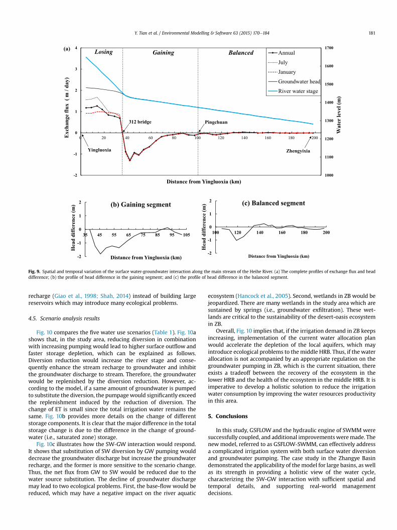
Fig. 9. Spatial and temporal variation of the surface water-groundwater interaction along the main stream of the Heihe River. (a) The complete profiles of exchange flux and headdifference; (b) the profile of head difference in the gaining segment; and (c) the profile of head difference in the balanced segment.

Y. Tian et al. / Environmental Modelling & Software 63 (2015) 170e184 181

recharge (Giao et al., 1998; Shah, 2014) instead of building largereservoirs which may introduce many ecological problems.

4.5. Scenario analysis results

Fig. 10 compares the five water use scenarios (Table 1). Fig. 10ashows that, in the study area, reducing diversion in combinationwith increasing pumping would lead to higher surface outflow andfaster storage depletion, which can be explained as follows.Diversion reduction would increase the river stage and conse-quently enhance the stream recharge to groundwater and inhibitthe groundwater discharge to stream. Therefore, the groundwaterwould be replenished by the diversion reduction. However, ac-cording to the model, if a same amount of groundwater is pumpedto substitute the diversion, the pumpagewould significantly exceedthe replenishment induced by the reduction of diversion. Thechange of ET is small since the total irrigation water remains thesame. Fig. 10b provides more details on the change of differentstorage components. It is clear that the major difference in the totalstorage change is due to the difference in the change of ground-water (i.e., saturated zone) storage.

Fig. 10c illustrates how the SW-GW interaction would respond.It shows that substitution of SW diversion by GW pumping woulddecrease the groundwater discharge but increase the groundwaterrecharge, and the former is more sensitive to the scenario change.Thus, the net flux from GW to SW would be reduced due to thewater source substitution. The decline of groundwater dischargemay lead to two ecological problems. First, the base-flow would bereduced, which may have a negative impact on the river aquatic

ecosystem (Hancock et al., 2005). Second, wetlands in ZB would bejeopardized. There are many wetlands in the study area which aresustained by springs (i.e., groundwater exfiltration). These wet-lands are critical to the sustainability of the desert-oasis ecosystemin ZB.

Overall, Fig. 10 implies that, if the irrigation demand in ZB keepsincreasing, implementation of the current water allocation planwould accelerate the depletion of the local aquifers, which mayintroduce ecological problems to themiddle HRB. Thus, if the waterallocation is not accompanied by an appropriate regulation on thegroundwater pumping in ZB, which is the current situation, thereexists a tradeoff between the recovery of the ecosystem in thelower HRB and the health of the ecosystem in the middle HRB. It isimperative to develop a holistic solution to reduce the irrigationwater consumption by improving the water resources productivityin this area.

5. Conclusions

In this study, GSFLOW and the hydraulic engine of SWMM weresuccessfully coupled, and additional improvements weremade. Thenew model, referred to as GSFLOW-SWMM, can effectively addressa complicated irrigation system with both surface water diversionand groundwater pumping. The case study in the Zhangye Basindemonstrated the applicability of themodel for large basins, as wellas its strength in providing a holistic view of the water cycle,characterizing the SW-GW interaction with sufficient spatial andtemporal details, and supporting real-world managementdecisions.

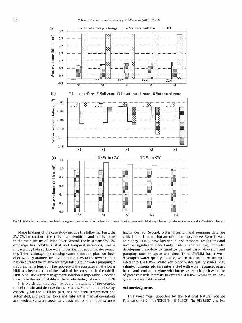
Fig. 10. Water balance in five simulated management scenarios (S0 is the baseline scenario). (a) Outflows and total storage changes; (b) storage changes; and (c) SW-GWexchanges.

Y. Tian et al. / Environmental Modelling & Software 63 (2015) 170e184182

Major findings of the case study include the following. First, theSW-GW interaction in the studyarea is significant andmainly occursin the main stream of Heihe River. Second, the in-stream SW-GWexchange has notable spatial and temporal variations, and isimpacted by both surface water diversion and groundwater pump-ing. Third, although the existing water allocation plan has beeneffective to guarantee the environmental flow to the lower HRB, ithas encouraged the relatively unregulated groundwater pumping inthis area. In the long-run, the recovery of the ecosystem in the lowerHRBmay be at the cost of the health of the ecosystem in the middleHRB. A holistic water management solution is imperatively neededto achieve the sustainability of the eco-hydrological system in HRB.

It is worth pointing out that some limitations of the coupledmodel remain and deserve further studies. First, the model setup,especially for the GSFLOW part, has not been streamlined andautomated, and external tools and substantial manual operationsare needed. Software specifically designed for the model setup is

highly desired. Second, water diversion and pumping data arecritical model inputs, but are often hard to achieve. Even if avail-able, they usually have low spatial and temporal resolutions andinvolve significant uncertainty. Future studies may considerdeveloping a module to simulate demand-based diversion andpumping rates in space and time. Third, SWMM has a well-developed water quality module, which has not been incorpo-rated into GSFLOW-SWMM yet. Since water quality issues (e.g.,salinity, nutrients, etc.) are interrelated with water resources issuesin arid and semi-arid regions with intensive agriculture, it would beof great research interests to extend GSFLOW-SWMM to an inte-grated water quality model.

Acknowledgments

This work was supported by the National Natural ScienceFoundation of China (NSFC) (No. 91125021, No. 91225301 and No.

Y. Tian et al. / Environmental Modelling & Software 63 (2015) 170e184 183

41371473). The data set was provided by Cold and Arid RegionsScience Data Center in Lanzhou, China (http://westdc.westgis.ac.cn). We also thank the three anonymous reviewers for theirinsightful comments and suggestions.

References

Adeboye, O.B., Osunbitan, J.A., Adekalu, K.O., Okunade, D.A., 2009. Evaluation ofFAO-56 PenmaneMonteith and temperature based models in estimatingreference evapotranspiration using complete and limited data, application toNigeria. Agric. Eng. Int. CIGR J. 11, 1e25.

Allen, R.G., Pereira, L.S., Raes, D., Smith, M., 1998. Crop Evapotranspiration-Guidelines for Computing Crop Water Requirements-FAO Irrigation andDrainage Paper 56. Food and Agriculture Organization of the United Nations,Rome, Italy.

Arnold, J.G., Srinivasan, R., Muttiah, R.S., Williams, J.R., 1998. Large area hydrologicmodeling and assessment part I: model development. JAWRA J. Am. WaterResour. Assoc. 34 (1), 73e89.

Barlow, P.M., DeSimone, L.A., Moench, A.F., 2000. Aquifer response to streamestageand recharge variations. II. Convolution method and applications. J. Hydrol. 230(3e4), 211e229.

Bennett, N.D., Croke, B.F.W., Guariso, G., Guillaume, J.H.A., Hamilton, S.H.,Jakeman, A.J., Marsili-Libelli, S., Newham, L.T.H., Norton, J.P., Perrin, C.,Pierce, S.A., Robson, B., Seppelt, R., Voinov, A.A., Fath, B.D., Andreassian, V., 2013.Characterising performance of environmental models. Environ. Model. Softw.40, 1e20.

Borah, D.K., Bera, M., 2003. Watershedescale hydrologic and nonpointesourcepollution models: review of mathematical bases. Trans. ASAE 46 (6),1553e1566.

Brunner, P., Simmons, C.T., 2012. HydroGeoSphere: a fully integrated, physicallybased hydrological model. Ground Water 50 (2), 170e176.

Chen, Z., Nie, Z., Zhang, G., Wan, L., Shen, J., 2006. Environmental isotopic study onthe recharge and residence time of groundwater in the Heihe River Basin,northwestern China. Hydrogeol. J. 14 (8), 1635e1651.

Cheng, G.D., Xiao, H.L., Zhao, W.Z., Feng, Q., Xu, Z.M., Li, X., 2009. Water-ecological-economic System Integrated Management Research on Heihe River Basin (inChinese). Science Press, Beijing.

Demetriou, C., Punthakey, J.F., 1998. Evaluating sustainable groundwater manage-ment options using the MIKE SHE integrated hydrogeological modelling pack-age. Environ. Model. Softw. 14 (2e3), 129e140.

Feng, Q., Cheng, G.D., 2001. Towards sustainable development of the environmen-tally degraded River Heihe basin, China. Hydro.Sci. 46 (5), 647e658.

Fisher, J.B., Whittaker, R.J., Malhi, Y., 2011. ET come home: potential evapotranspi-ration in geographical ecology. Glob. Ecol. Biogeogr. 20 (1), 1e18.

Giao, P.H., PhieneWej, N., Honjo, Y., 1998. FEM quasi-3D modelling of responses toartificial recharge in the Bangkok multiaquifer system. Environ. Model. Softw.14 (2e3), 141e151.

Gilfedder, M., Rassam, D.W., Stenson, M.P., Jolly, I.D., Walker, G.R., Littleboy, M., 2012.Incorporating land-use changes and surfaceegroundwater interactions in asimple catchment water yield model. Environ. Model. Softw. 38, 62e73.

Giron�as, J., Roesner, L.A., Rossman, L.A., Davis, J., 2010. A new applications manualfor the Storm Water Management Model (SWMM). Environ. Model. Softw. 25(6), 813e814.

Graham, D.N., Butts, M.B., 2005. Flexible, integrated watershed modelling withMIKE SHE. In: V.P., S., D.K., F (Eds.), Watershed Models. CRC Press, pp. 245e272.

Guo, Q., Feng, Q., Li, J., 2009. Environmental changes after ecological waterconveyance in the lower reaches of Heihe River, northwest China. Environ. Geol.58 (7), 1387e1396.

Hancock, P., Boulton, A., Humphreys, W., 2005. Aquifers and hyporheic zones: to-wards an ecological understanding of groundwater. Hydrogeol. J. 13 (1), 98e111.

Harbaug, A.W., 2005. MODFLOWe2005. The U.S. Geological Survey modulargroundwater model-the ground-water flow process. USGS Techniques andMethods: 6eA16. Available at: http://pubs.usgs.gov/tm/2005/tm6A16/PDF.htm(accessed 07.03.14.).

Hu, L., Chen, C., Jiao, J.J., Wang, Z., 2007. Simulated groundwater interaction withrivers and springs in the Heihe river basin. Hydrol. Process. 21 (20), 2794e2806.

Hu, X., Xiao, H., Lan, Y., 2012. Experimental study of calculating method of riverSeepagein middle and upper reaches of the heihe river (in chinese). J. Glaciol.Geocryol. 2, 460e468.

Huntington, J.L., Niswonger, R.G., 2012. Role of surfaceewater and groundwaterinteractions on projected summertime streamflow in snow dominated regions:an integrated modeling approach. Water Resour. Res. 48 (11), W11524.

Leavesley, G.H., Lichty, R.W., Troutman, B.M., Saindon, L.G., 1983. Precip-itationerunoff Modeling System; User's Manual USGS Watereresources In-vestigations Report. USGS WatereResources Investigations Report: 83e4238,206pp. Available at: http://pubs.usgs.gov/wri/1983/4238/report.pdf (accessed07.03.14.).

Li, X., Cheng, G., Liu, S., Xiao, Q., Ma, M., Jin, R., Che, T., Liu, Q., Wang, W., Qi, Y.,Wen, J., Li, H., Zhu, G., Guo, J., Ran, Y., Wang, S., Zhu, Z., Zhou, J., Hu, X., Xu, Z.,2013. Heihe Watershed Allied Telemetry Experimental Research (HiWATER):scientific objectives and experimental design. Bull. Am. Meteorol. Soc. 94 (8),1145e1160.

Li, X.M., Lu, L., Yang, W.F., Cheng, G.D., 2012. Estimation of evapotranspiration in anarid region by remote sensingdA case study in the middle reaches of the HeiheRiver Basin. Int. J. Appl. Earth Obs. Geoinform. 17, 85e93.

Li, Z., Shao, Q., Xu, Z., Cai, X., 2010. Analysis of parameter uncertainty in semi-edistributed hydrological models using bootstrap method: a case study ofSWAT model applied to Yingluoxia watershed in northwest China. J. Hydrol. 385(1e4), 76e83.

Liu, W., Cao, S., Xi, H., Feng, Q., 2010. Land use history and status of land deserti-fication in the Heihe River basin. Nat. Hazards 53 (2), 273e290.

Luo, F., Qi, S.Z., Xiao, H.L., 2005. Landscape change and sandy desertification in aridareas: a case study in the Zhangye Region of Gansu Province, China. Environ.Geol. 49, 90e97.

Markstrom, S.L., 2012. Integrated Watershedescale Response to Climate Change forSelected Basins across the United States. U.S. Geological Survey Scientific In-vestigations Report 2011e5077, 143pp. Available at: http://pubs.usgs.gov/sir/2011/5077/SIR11-5077_508.pdf (accessed 07.03.14.).

Markstrom, S.L., Niswonger, R.G., Regan, R.S., Prudic, D.E., Barlow, P.M., 2008.GSFLOWeCoupled Groundewater and Surfaceewater FLOW Model Based onthe Integration of the Precipitationerunoff Modeling System (PRMS) and theModular Groundewater FlowModel (MODFLOWe2005). U.S. Geological SurveyTechniques and Methods 6eD1, 240pp. Available at: http://pubs.usgs.gov/tm/tm6d1/pdf/tm6d1.pdf (accessed 07.03.14.).

McCallum, A.M., Andersen, M.S., Giambastiani, B.M.S., Kelly, B.F.J., Ian Acworth, R.,2013. Rivereaquifer interactions in a semiearid environment stressed bygroundwater abstraction. Hydrol. Process. 27 (7), 1072e1085.

Nalder, I.A., Wein, R.W., 1998. Spatial interpolation of climatic Normals: test of anew method in the Canadian boreal forest. Agric. For. Meteorol. 92 (4),211e225.

Nash, J.E., Sutcliffe, J.V., 1970. River flow forecasting through conceptual models partI d a discussion of principles. J. Hydrol. 10 (3), 282e290.

Niswonger, R.G., Prudic, D.E., 2005. Documentation of the Streamflowerouting (SFR2)Package to Include Unsaturated Flow beneath Streamsda Modification to SFR1.U.S. Geological Survey Techniques and Methods 6eA13, 50 pp. Available at:http://pubs.usgs.gov/tm/2006/tm6A13/pdf/tm6a13.pdf (accessed 07.03.14.).

Niswonger, R.G., Prudic, D.E., Fogg, G.E., Stonestrom, D.A., Buckland, E.M., 2008.Method for estimating spatially variable seepage loss and hydraulic conductivityin intermittent and ephemeral streams. Water Resour. Res. 44 (5), W05418.

Niswonger, R.G., Prudic, D.E., Regan, R.S., 2006. Documentation of the Unsatur-atedezone Flow (UZF1) Package for Modeling Unsaturated Flow between theLand Surface and the Water Table with MODFLOWe2005. U.S. Geological Sur-vey Techniques and Methods, 6eA19, 62 pp. Available at: http://pubs.usgs.gov/tm/2006/tm6a19/pdf/tm6a19.pdf (accessed 07.03.14).

P�erez, A.J., Abrah~ao, R., Causap�e, J., Cirpka, O.A., Bürger, C.M., 2011. Simulating thetransition of a semiearid rainfed catchment towards irrigation agriculture.J. Hydrol. 409 (3e4), 663e681.

Panday, S., Huyakorn, P.S., 2004. A fully coupled physicallyebased spa-tiallyedistributed model for evaluating surface/subsurface flow. Adv. WaterResour. 27 (4), 361e382.

Peterson, E.W., Wicks, C.M., 2006. Assessing the importance of conduit geometryand physical parameters in karst systems using the storm water managementmodel (SWMM). J. Hydrol. 329 (1e2), 294e305.

Rassam, D.W., 2011. A conceptual framework for incorporating surfaceeground-water interactions into a river operationeplanning model. Environ. Model.Softw. 26 (12), 1554e1567.

Rassam, D.W., Peeters, L., Pickett, T., Jolly, I., Holz, L., 2013. Accounting for surfa-ceegroundwater interactions and their uncertainty in river and groundwatermodels: a case study in the Namoi River, Australia. Environ. Model. Softw. 50(0), 108e119.

Rossman, L.A., 2009. Storm Water Management Model User's Manual Version 5.0.U.S.. Environmental Protection Agency, EPA/600/R-05/040. Available at: http://nepis.epa.gov/Adobe/PDF/P10011XQ.pdf (accessed 07.03.14.).

Rodriguez, L.B., Cello, P.A., Vionnet, C.A., Goodrich, D., 2008. Fully conservativecoupling of HECeRAS with MODFLOW to simulate streameaquifer interactionsin a drainage basin. J. Hydrol. 353 (1e2), 129e142.

Shah, T., 2014. Towards a Managed Aquifer Recharge strategy for Gujarat, India: aneconomist's dialogue with hydroegeologists. J. Hydrol. 518, 94e107.

Shrestha, N.K., Leta, O.T., De Fraine, B., van Griensven, A., Bauwens, W., 2013.OpenMIebased integrated sediment transport modelling of the river Zenne,Belgium. Environ. Model. Softw. 47 (0), 193e206.

Siebert, S., Burke, J., Faures, J.M., Frenken, K., Hoogeveen, J., D€oll, P., Portmann, F.T.,2010. Groundwater use for irrigation e a global inventory. Hydrol. Earth Syst.Sci. Discuss. 7 (3), 3977e4021.

Singh, V.P., 2001. Kinematic wave modelling in water resources: a historicalperspective. Hydrol. Process. 15 (4), 671e706.

Sophocleous, M., 2002. Interactions between groundwater and surface water: thestate of the science. Hydrogeol. J. 10 (1), 52e67.

Sophocleous, M.A., Koelliker, J.K., Govindaraju, R.S., Birdie, T., Ramireddygari, S.R.,Perkins, S.P., 1999. Integrated numerical modeling for basinewide water man-agement: the case of the Rattlesnake Creek basin in southecentral Kansas.J. Hydrol. 214 (1e4), 179e196.

Therrien, R., McLaren, R.G., Sudicky, E.A., Panday, S.M., 2010. HydroGeoSphere AThreeedimensional Numerical Model Describing Fullyeintegrated Subsurfaceand Surface Flow and Solute Transport. Technical report.

Valerio, A., Rajaram, H., Zagona, E., 2010. Incorporating GroundwatereSurface waterinteraction into river management models. Ground Water 48 (5), 661e673.

Y. Tian et al. / Environmental Modelling & Software 63 (2015) 170e184184

VanderKwaak, J.E., Loague, K., 2001. HydrologiceResponse simulations for the Re5catchment with a comprehensive physicsebased model. Water Resour. Res. 37(4), 999e1013.

Vieira, J.H.D., 1983. Conditions governing the use of approximations for theSainteV�enant equations for shallow surface water flow. J. Hydrol. 60 (1e4),43e58.

Wang, X.S., Ma, M.G., Li, X., Zhao, J., Dong, P., Zhou, J., 2010. Groundwater responseto leakage of surface water through a thick vadose zone in the middle reachesarea of Heihe River Basin, in China. Hydrol. Earth Syst. Sci. 14 (4), 639e650.

Welsh, W.D., Vaze, J., Dutta, D., Rassam, D., Rahman, J.M., Jolly, I.D., Wallbrink, P.,Podger, G.M., Bethune, M., Hardy, M.J., Teng, J., Lerat, J., 2013. An integratedmodelling framework for regulated river systems. Environ. Model. Softw. 39 (0),81e102.

Wen, X.H., Wu, Y.Q., Lee, L.J.E., Su, J.P., Wu, J., 2007. Groundwater flow modeling inthe Zhangye Basin, northwestern China. Environ. Geol. 53 (1), 77e84.

Werner, A.D., Gallagher, M.R., Weeks, S.W., 2006. Regionalescale, fully coupledmodelling of streameaquifer interaction in a tropical catchment. J. Hydrol. 328(3e4), 497e510.

Wu, Y.Q., Zhang, Y.H., Wen, X.H., Su, J.P., 2010. Hydrologic Cycle and Water ResourceModeling for the Heihe River Basin in Northwestern China (in Chinese). SciencePress, Beijing.

Zhang, G.H., Liu, S.Y., Xie, Y.B., 2004. Water Cycle and Development of Groundwaterin the Inland Heihe River Basin InWesteNorth China (in Chinese). GeologyPublication House, Beijing.