Modeling space-time data using stochastic diﬁerential

Bayesian Analysis (2009) 4, Number 4, pp. 733–758

Modeling space-time data using stochasticdifferential equations

Jason A. Duan∗, Alan E. Gelfand† and C. F. Sirmans‡

Abstract. This paper demonstrates the use and value of stochastic differentialequations for modeling space-time data in two common settings. The first consistsof point-referenced or geostatistical data where observations are collected at fixedlocations and times. The second considers random point pattern data where theemergence of locations and times is random. For both cases, we employ stochas-tic differential equations to describe a latent process within a hierarchical modelfor the data. The intent is to view this latent process mechanistically and endowit with appropriate simple features and interpretable parameters. A motivatingproblem for the second setting is to model urban development through observedlocations and times of new home construction; this gives rise to a space-time pointpattern. We show that a spatio-temporal Cox process whose intensity is drivenby a stochastic logistic equation is a viable mechanistic model that affords mean-ingful interpretation for the results of statistical inference. Other applications ofstochastic logistic differential equations with space-time varying parameters in-clude modeling population growth and product diffusion, which motivate our first,point-referenced data application. We propose a method to discretize both timeand space in order to fit the model. We demonstrate the inference for the geosta-tistical model through a simulated dataset. Then, we fit the Cox process modelto a real dataset taken from the greater Dallas metropolitan area.

Keywords: geostatistical data, point pattern, hierarchical model, stochastic logisticequation, Markov chain Monte Carlo, urban development

1 Introduction

The contribution of this paper is to demonstrate the use and value of stochastic dif-ferential equations (SDE) to yield mechanistic and physically interpretable models forspace-time data. We consider two common settings: (i) real-valued and point-referencedgeostatistical data where observations are taken at non-random locations s and timest and (ii) spatio-temporal point patterns where the locations and times themselves arerandom. In either case, we assume s ∈ D ⊂ R2 where D is a fixed compact region andt ∈ (0, T ] where T is specified.

Examples of spatio-temporal geostatistical data abound in the literature. Examplesappropriate to our objectives include ecological process models such as photosynthesis,

∗Department of Marketing, McCombs School of Business,University of Texas, Austin, TX, mailto:[email protected]

†Department of Statistical Science, Duke University, Durham, NC mailto:[email protected]‡Department of Risk Management, Insurance, Real Estate and Business Law, Florida State Univer-

sity, Tallahassee, FL mailto:[email protected]

c© 2009 International Society for Bayesian Analysis DOI:10.1214/09-BA427

mailto:[email protected]




734 Space-time SDE models

transpiration, and soil moisture; diffusion models for populations, products or technolo-gies; financial processes such as house price and/or land values over time. Here, weemploy a customary geostatistical modeling specification, i.e., noisy space-time dataare modeled by

Y (s, t) = Λ(s, t) + ε(s, t) (1)where ε(s, t) is a space-time noise/error process (contributing the “nugget”) and theprocess of interest is Λ(s, t). For us, Λ(s, t) is a realization of a space-time stochasticprocess generated by a stochastic differential equation.

Space-time point patterns also arise in many settings, e.g., ecology where we mightseek the evolution of the range of a species over time by observing the locations of itspresences; disease incidence examining the pattern of cases over time; urban develop-ment explained using say the pattern of single family homes constructed over time. Therandom locations and times of these events are customarily modeled with an inhomo-geneous intensity surface denoted again by Λ(s, t). Here, the theory of point processesprovides convenient tools; the most commonly used and easily interpretable model isthe spatio-temporal Poisson process: for any region in the area under study and anyspecified time interval, the total number of observed points is a Poisson random variablewith mean equal to the integrated intensity over that region and time interval.

There is a substantial literature on modeling point-referenced space-time data. Themost common approach is the introduction of spatio-temporal random effects describedthrough a Gaussian process with a suitable space-time covariance function (e.g., Brownet al. 2000; Gneiting 2002; Stein 2005). If time is discretized, we can employ dynamicmodels as in Gelfand et al. (2005). If locations are on a lattice (or are projected toa lattice), we can employ Gaussian Markov random fields (Rue and Held 2005). Forgeneral discussion of such space-time modeling see Banerjee et al. (2004).

There is much less statistical literature on space-time point patterns. However, themathematical theory of point process on a general carrying space is well established(Daley and Vere-Jones 1988; Karr 1991). Cressie (1993) and Møller and Waagepetersen(2004) focus primarily on two-dimensional spatial point processes. Recent developmentsin spatio-temporal point process modeling include Ogata (1998) with application tostatistical seismology and Brix and Møller (2001) with application in modeling weeds.Brix and Diggle (2001), in modeling a plant disease, extend the log Gaussian Cox process(Møller et al. 1998) to a space-time version by using a stochastic differential equationmodel. See Diggle (2005) for a comprehensive review of this literature.

In either of the settings (i) and (ii) above, we propose to work with stochastic dif-ferential equation models. That is, we intentionally specify Λ (s, t) through a stochasticdifferential equation rather than a spatio-temporal process (see, e.g., Banerjee et al.2004 and references therein). We specifically introduce a mechanistic modeling schemewhere we are directly interested in the parameters that convey physical meanings in themechanism described by a stochastic differential equation. For example, the prototypeof our study is the logistic equation

∂Λ (s, t)∂t

= r(s, t)Λ (s, t)[1− Λ (s, t)

K (s)

],

J. A. Duan, A. E. Gelfand and C. F. Sirmans 735

where K (s) is the “carrying capacity” (assuming it is time-invariant) and r (s, t) isthe “growth rate”. Spatially and/or temporally varying parameters, such as growthrate and carrying capacity, can be modeled by spatio-temporal processes. In practice,the logistic equation finds various applications, e.g., population growth in ecology (Kot2001), product and technology diffusion in economics (Mahajan and Wind 1986), andurban development (see Section 4.2).

We recognize the flexibility that comes with a “purely empirical” model such as arealization of a stationary or nonstationary space-time Gaussian process or smoothingsplines and that such specifications can be made to fit a given dataset at least as wellas a specification limited to a given class of stochastic differential equations. However,for space-time data collected from physical systems it may be preferable to view themas generated by appropriate simple mechanisms with necessary randomness. That is,we particularly seek to incorporate the features of the mechanistic process into themodel for the space-time data enabling interpretation of the spatio-temporal parameterprocesses that is more natural and intuitive. We also demonstrate, through a simulationexample, that, when such differential equations generate the data (up to noise), thedata can inform about the parameters in these equations and that model performanceis preferable to that of a customary model employing a random process realization.

In this regard, we must resort to discretization of time to work with these models,i.e., we actually fit stochastic finite difference models. In other words, the continuous-time specification describes the process we seek to capture but to fit this specificationwith observed data, we employ first order (Euler) approximation. Evidently, this raisesquestions regarding the effect of discretization. Theoretical discussion in terms of weakconvergence is presented, for instance, in Kloeden and Platen (1992) while practicalrefinements through latent variables have been proposed in, e.g., Elerian et al. (2001).In any event, Euler approximation is widely applied in the literature and it is beyond ourcontribution here to explore its impact. Moreover, the results of our simulation examplein Section 3.3 reveal that we recover the true parameters of the stochastic PDE quitewell under the discretization.

Indeed, the real issue for us is how to introduce randomness into a selected differentialequation specification. Section 2 is devoted to a brief review of available options andtheir associated properties. Section 3 develops the geostatistical setting and providesthe aforementioned simulation illustration.

An early motivating problem for our research was the modeling of new home con-structions in a fixed region, e.g., within a city boundary. Mathematically and concep-tually, the continuous trend that drives the construction of new houses can be capturedby the logistic equation, where there is a rate for the growth of the number of housesand a carrying capacity that limits the total number. When new houses can be built atany locations and times, yielding a space-time point pattern, a spatio-temporal pointprocess governed by a version of the stochastic logistic equation becomes an appealingmechanistic model. However, we also acknowledge its limitations, suggesting possibleextensions at the end of the paper.

Section 4.1 details the modeling for space-time point patterns and addresses formal


modeling and computational issues. Section 4.2 provides a careful analysis of the houseconstruction dataset. Finally, in Section 5, we conclude with a summary and somefuture directions.

2 SDE models for spatio-temporal data

Ignoring location for the moment, a usual nonlinear (non-autonomous) differential equa-tion subject to the initial condition takes the form

dΛ(t) = g(Λ(t), t, r (t))dt and Λ (0) = Λ0. (2)

A natural way to add randomness is to model the random parameter r (t) with aSDE:

dr (t) = a(r(t), t, β)dt + b (r (t) , t) dB (t)

where B(t) is an independent-increment process on R1.1

Analytic solutions of SDE’s are rarely available so we usually employ a first orderEuler approximation of the form,

Λ (t + ∆t) = Λ (t) + g(Λ (t) , t, r (t))∆t

and r (t + ∆t) = r (t) + a(r(t), t, β)∆t + b (r (t) , t) [B (t + ∆t)−B (t)]

where ∆t is the interval between time points and B (t + ∆t)−B (t) ∼ N(0, ∆t) if B(t)is a Brownian motion process. Higher order (Runge-Kutta) approximations can beintroduced but these do not seem to be employed in the statistics literature. Rather,recent work introduces latent variables Λ(t′)’s between Λ(t) and Λ(t + ∆t). See, e.g.,Elerian et al. (2001); Golightly and Wilkinson (2008) and Stramer and Roberts (2007).

Our prototype is the logistic equation

dΛ (t) = r(t)Λ (t)[1− Λ (t)

K

]dt and Λ (0) = Λ0. (3)

To introduce systematic randomness into this model, we specify a mean-revertingOrnstein-Uhlenbeck process for r (t):

dr (t) = −α (µr − r (t)) dt + σζdB (t) . (4)

Under Brownian motion it is known that r (t) is a stationary Gaussian process withcov(r (t) , r (t′)) = (σ2

ζ/α) exp (−α|t− t′|).To extend model (3) to a spatio-temporal setting, we can model Λ (s, t) at every

location s with a SDE∂Λ (s, t)

∂t= r(s, t)Λ (s, t)

[1− Λ (s, t)

K (s)

](5)

1This is a very general specification. For example, a common SDE model is dΛ(t) = f(Λ(t), t)dt +h(Λ(t), t)dB(t) where B(t) is Brownian motion over R1 with f and h the “drift” and “volatility” respec-tively. This model can be considered as model (2) with g (Λ (t) , t, r (t)) = f (Λ (t) , t) + r (t) h (Λ (t) , t)and dr (t) = r (t) dt = dB (t), which implies dΛ(t) = f(Λ(t), t)dt + h (Λ (t) , t) dB(t).


subject to the initial conditions Λ (s, 0) = Λ0 (s). Expression (5) is derived directly from(3) as follows. Assume model (3) for the aggregate Λ (D, t) =

∫D

Λ (s, t) ds:

∂Λ (D, t)∂t

= r(D, t)Λ (D, t)[1− Λ (D, t)

K (D)

]. (6)

Here r (D, t) is the average growth rate of Λ (D, t), i.e., r (D, t) = (∫

Dr (s, t) ds)/|D|

where |D| is the area of D. K(D) is the aggregate carrying capacity, i.e., K (D) =∫D

K (s) ds.

The model for Λ (s, t) at any location s can be considered as the infinitesimal limitof the model (6) when D is a neighborhood, δs of s whose area goes to zero. Then,

lim|δs|→0

Λ (δs, t) / |δs| = lim|δs|→0

(∫

δs

Λ (s′, t) ds′)/ |δs| = Λ (s, t) ;

lim|δs|→0

K (δs) / |δs| = lim|δs|→0

(∫

δs

K (s′) ds′)/ |δs| = K(s);

lim|δs|→0

r(δs, t) = lim|δs|→0

∫

δs

r (s′, t) ds′/|δs| = r (s, t) .

Plugging δs into (6) and passing to the limit, we obtain our local model (5).

Model (5) specifies an infinite-dimensional SDE model for the random field Λ (s, t) ,s ∈ D. Similar to (4), we can add randomness to (5) by extending the Ornstein-Uhlenbeck process to the case of infinite dimension,

∂r (s, t)∂t

= L (µr (s)− r(s, t)) +∂B (s, t)

∂t, (7)

where L (s) is a spatial linear operator given by

L (s) = a (s) +2∑

l=1

bl (s)∂

∂sl− 1

2

2∑

l=1

cl (s)∂2

∂s2l

(8)

where a (s), bl (s) and cl (s) are positive deterministic functions with s1 and s2 thecoordinates of location s. B (s, t) is a spatially correlated Brownian motion. Here,equation (5) and (7) define a spatio-temporal model with a nonstationary and non-Gaussian Λ (s, t) and a latent stationary Gaussian r (s, t). Note that a well-specifiedCB will guarantee mean-square continuity and differentiability of r (s, t), s ∈ D. Be-cause the logistic equation is Lipschitz, Λ (s, t) will also be mean-square continuous anddifferentiable.

The simplest Ornstein-Uhlenbeck process model for r (s, t) sets bl and cl to zero (seeBrix and Diggle 2001); the resulting covariance is separable in space and time. Forexample, with the Matern spatial covariance function, we have

Cr(s− s′, t− t′) = σ2 exp (−a |t− t′|) (φζ |s− s′|)νκν (φζ |s− s′|) , (9)


where κν (·) is the modified Bessel function of the second kind. When bl and cl are notequal to zero, r (s, t) defined by equation (7) is a blur-generated process in Brown et al.(2000) with a nonseparable non-explicit spatio-temporal covariance function. Whittle(1963) and Jones and Zhang (1997) propose other stochastic partial differential equationmodels, which are shown by Brown et al. (2000) to be special examples of the Ornstein-Uhlenbeck process model above.

Returning to the discussion in the Introduction, conceptually, Λ (s, tj) is generatedby the continuous-time process defined by (5) and (7). However, the exact solution ofthis infinite-dimensional SDE and the transition probability of the resulting Markov pro-cess for Λ (s, tj) are not generally known in closed-form given the error process B (s, t).Hence, for handling these models, time-discretization is usually required to computeΛ (s, t) in simulation and estimation. So, we use Euler approximation to discretize theSDE model for Λ (s, tj) . The Euler scheme is broadly employed in simulating SDE’sbecause it the simplest method that is proven to generate a stochastic process that hasboth strong convergence of order 1/2 and weak convergence of order 1 (see Kloedenand Platen 1992 for theoretical discussions). That is the stochastic difference equationresulting from the Euler discretization scheme generates a process that will converge tothe process defined by the stochastic differential equation when the length of time stepsgoes to zero.

3 Geostatistical models using SDE

3.1 A discretized space-time model with white noise

We assume time is discretized to small, equally spaced intervals of length ∆t, indexed astj , j = 0, 1, ..., J . The data is considered to be Y (si, tj), i.e., an observation at locations and any t ∈ (tj , tj + ∆t) is labeled as Y (s, tj). Then, we assume

Y (s, tj) = Λ (s, tj) + ε (s, tj) ,

where ε (s, tj) models either sampling or measure errors because a researcher cannotdirectly observe Λ (s, tj).

The dynamics of the discretized Λ (s, tj) is therefore modeled by a difference equationusing Euler’s approximation applied to (5):

∆Λ (s, tj) = r(s, tj−1)Λ (s, tj−1)[1− Λ (s, tj−1)

K (s)

]∆t, (10)

Λ (s, tj) ≈ Λ (s, 0) +j∑

l=1

∆Λ(s, tj−1) . (11)

We do not have to discretize the space-time model for r (s, t) if the stationary spatio-temporal Gaussian process ζ (s, t) allows direct evaluation of its covariance function.For example, the model (7) with constant L (s) = ar has the closed-form separable


covariance function given in (9) which can be directly used in modeling and can beestimated. Using this form saves one approximation step.

We still need to model the initial Λ (s, 0) and K (s) if they are not known. Forexample, because Λ (s, 0) and K (s) are positive in the logistic equation, we can modelthem by the log-Gaussian spatial processes with regression forms for the means,

log Λ (s, 0) = µΛ (XΛ (s) , βΛ) + θΛ (s) , θΛ (s) ∼ GP(0, CΛ (s− s′; ϕΛ)) ;log K (s) = µK (XK (s) , βK) + θK (s) , θK (s) ∼ GP(0, CK (s− s′; ϕK)) .

Similarly, µr(s) below (7) can be modeled as µr (Xr (s) , βr).

Conditioned on Λ (s, tj), the Y (s, tj) are mutually independent. With data Y (si, tj)at locations si, i = 1, . . . , n ⊂D, we can provide a hierarchical model based on theevolution of Λ (s, t) and the space-time parameters. We fit this model within a Bayesianframework so completion of the model specification requires introduction of suitablepriors on the hyper-parameters.

For simplicity, we suppress the indices t and s and let our observations at time tj beyj = yj1, . . . , yjn at the corresponding s1, . . . , sn locations. Accordingly, we let Λj ,∆Λj , rj , K, µΛ (βΛ), µK (βK), µr (βr), θΛ, θK and ζ be the vectors of the correspondingfunctions and processes in our continuous model evaluated at si ∈ s1, . . . , sn. Notethat we begin with the initial observations y0. The hierarchical model for y0, . . . , yJ

becomesyj |Λj ∼ N

(Λj , σ

2εIn

), j = 0, . . . , J,

∆Λj = rj−1Λj−1

[1− Λj−1

K

]∆t,

Λj = Λ0 +j−1∑

l=1

∆Λl,

log Λ0 = µΛ (βΛ) + θΛ, θΛ ∼ N (0, CΛ (s− s′; ϕΛ)) ,

log K = µK (βK) + θK , θK ∼ N (0, CK (s− s′; ϕK)) ,

r = µr (βr) + ζ, ζ ∼ N (0, Cr(s− s′, t− t′; ϕr)) ,

βΛ, βr, βK , ϕΛ, ϕK , ϕr ∼ priors,

(12)

where β(·) are the parameters in the mean surface function; CΛ, CK and Cr2 are the

covariance matrices. In this model, Λ0, r and K are latent variables. Note that theΛj ’s are deterministic functions of Λ0, r and K. The joint likelihood for the J + 1conditionally independent observations and latent variables is

J∏

j=0

N

(yj |Λj (Λj−1, rj ,K) , σ2

εIn

)N (log Λ0|µΛ, CΛ) N (log K|µK , CK) N (r|µr, Cr) ,

(13)where we let r = r0, . . . , rJ−1.

2We will write µΛ (βΛ), µK (βK),

µ(j)r (βr) ; j = 1, . . . , J

, CΛ (ϕΛ), CK (ϕK) and Cr (ϕr) as µΛ,

µK , µr, CΛ, CK and Cr when there is no ambiguity.


3.2 Bayesian inference and prediction

With regard to inference for the model in (12), there are three latent vectors: r, K andΛ0. The hyper-parameters in this model include the βr, βK and βΛ in the parametrictrend surfaces, the spatial random effects ζ, θK , θΛ and the hyper-parameters ϕr, ϕK ,ϕΛ in the covariance functions.

The priors for the hyper-parameters are assumed to have the form

βr, βK , βΛ ∼ π (βr) · π (βK) · π (βΛ) ; ϕr, ϕK , ϕΛ ∼ π (ϕr) · π (ϕK) · π (ϕΛ) (14)

where each of βr, βK , βΛ, ϕr, ϕK , ϕΛ may represent multiple parameters. For example,we have ϕr =

αr, φr, σ

2r , ν

in the Matern class covariance function for the separable

model (9). Exact specifications of the priors for the β’s and ϕ’s depend on the particularapplication. For example, if we take µr(s; βr) =X (s)βr, we adopt a weak normal priorN (0, Σβ) for βr. The parameter σ2

r receives the usual Inverse-Gamma prior. Note that∆Λj in the likelihood (13) for the discretized model are deterministic functions of r, Kand Λ0 defined by (10) and (11). Therefore the joint posterior is proportional to

J∏

j=0

N

(yj |Λj (Λj−1, rj ,K) , σ2

εIn

)N (log Λ0|µΛ, CΛ) N (log K|µK , CK) N (r|µr, Cr) ·

π (βr)π (βK) π (βΛ)π (ϕr) π (ϕK)π (ϕΛ) .

(15)

We simulate the posterior distributions of the model parameters and latent variablesin (15) using a Markov Chain Monte Carlo algorithm. Because the intensities in thelikelihood function are irregular recursive and nonlinear functions of the model param-eters and latent variables, it is very difficult to obtain derivatives for an MCMC withdirectional moves, such as the Langevin method. So, instead we use a random-walkMetropolis-Hastings algorithm in the posterior simulation. Each parameter is updatedin turn in every iteration of the simulation.

The prediction problem concerns (i) interpolating the past at new locations and (ii)forecasting the future at current and new locations. Indeed, we can hold out the ob-served data at new locations or in a future time period to validate our model. For thelogistic growth function, conditioning on the posterior samples of Λ0, K, r and βr, βK ,βΛ, ϕr, ϕK , ϕΛ, we can use spatio-temporal interpolation and temporal extrapolationto obtain ∆ΛJ+∆J (s) in period J + ∆J at any new location s ∈ D by calculatingµr (s, βr), µK (s, βK), µΛ (s, βΛ) and obtaining ζ(t, s), t = 1, . . . , J + ∆J , θK (s) andθΛ (s) by spatio-temporal prediction, and then using (10) and (11) recursively. Becausewe can obtain a predictive sample for ∆ΛJ+∆J (s) from the posterior samples of themodel fitting, we can infer on any feature of interest associated with the predictivedistribution of ∆ΛJ+∆J (s). The spatial interpolation of past observations at new loca-tions is demonstrated in the subsection below using a simulated example. We will alsodemonstrate temporal prediction when we apply a Cox-process version of our model tothe house construction data in Section 4.


3.3 A simulated data example

In order to see how well we can learn about the true process, we illustrate the fitting ofthe models in (12) with a simulated data set. In a study region D of 10×10 square unitsshown as the block in Figure 1, we simulate 44 locations at which spatial observations arecollected over 30 periods. Therefore our observed spatio-temporal data that constitutea 44×30 matrix. The data are sampled using (12) where we fix the carrying capacity tobe one at all locations. We may envision that the data simulate the household adoptionrates for a certain durable product (e.g., air conditioners, motorcycles) in 44 citiesover 30 months. A capacity of one means 100% adoption. Household adoption rates arecollected by surveys with measurement errors. The initial condition Λ0 is simulated as alog-Gaussian process with a constant mean surface µΛ and the Matern class covariancewhose smoothness parameter ν is set to be 3/2. The spatio-temporal growth rater is simulated using a constant mean µr and the separable covariance function (9),where the Matern smoothness parameter ν is also set to be 3/2. This separable modelinduces a convenient covariance matrix as the Kronecker product of the temporal andspatial correlation matrices: σ2

rΣt⊗Σs. The values of the fixed parameters in our datasimulation are presented in Table 1.

Model Parameters True Value Posterior Mean 95% Equal-tail IntervalµΛ -4.2 -4.14 (-4.88, -3.33)σΛ 1.0 0.91 (0.62, 1.46)φΛ 0.7 0.77 (0.50, 1.20)σε 0.05 0.049 (0.047, 0.052)µr 0.24 0.24 (0.22, 0.26)σr 0.08 0.088 (0.077, 0.097)φr 0.7 0.78 (0.60, 1.10)αr 0.6 0.64 (0.51, 0.98)

Table 1: Parameters and their posterior inference for the simulated example

We use the simulated r and Λ0 and the transition equation (10) recursively to obtain∆Λj and Λj for each of the 30 periods. The observed data yj are sampled as mutuallyindependent given Λj with the random noise εj . The data at four selected locations(marked as 1, 2, 3, and 4 in Figure 1) are shown as small circles in Figure 2. We leaveout the data at four randomly chosen locations (shown in diamond shape and markedas A, B, C and D in Figure 1) for spatial prediction and out-of-sample validation forour model.

We fit the same model (12) to the data at the remaining 40 locations (hence a40×30 spatio-temporal data set). We use very vague priors for the constant means:π(µΛ) ∼ N

(0, 108

)and π (µr) ∼ N

(0, 108

). We use natural conjugate priors for the

precision parameters (inverse of variances) of r and Λ0: π(1/σ2

r

) ∼ Gamma(1, 1) andπ

(1/σ2

Λ

) ∼ Gamma(1, 1). The positive parameter for the temporal correlation of r

also has a vague log-normal prior: π (αr) ∼ log-N(0, 108

). Because the spatial range

parameters φr and φΛ are only weakly identified (Zhang 2004), we only use informative


and discrete prior for them. Indeed we have chosen 20 values (from 0.1 to 2.0) andassume uniform priors on them for both φr and φΛ.

We use the random-walk Metropolis-Hastings algorithm to simulate posterior sam-ples of r and Λ0. We draw the entire vector of Λ0 for all forty locations as a single blockin every iteration. Because r is very high-dimensional (r being a 40×30 matrix), wecannot draw the entire matrix of r as one block and have satisfactory acceptance rate(between 20% to 40%). Our algorithm divides r into 40 row blocks (location-wise) inevery odd-numbered iteration and 30 column blocks (period-wise) in every even num-bered iteration. Each block is drawn in one Metropolis step. We find the posteriorsamples start to converge after about 30,000 iterations. Given the sampled r and Λ0,the mean parameters µr, µΛ and the precision parameters 1/σ2

r and 1/σ2Λ all have con-

jugate priors, and therefore their posterior samples are drawn with Gibbs samplers. φr

and φΛ have discrete priors and therefore discrete Gibbs samplers too. We also use therandom-walk Metropolis-Hastings algorithm to draw αr.

We obtain 200,000 samples from the algorithm and discard the first 100,000 as burn-in. For the posterior inference, we use 4,000 subsamples from the remaining 100,000samples, with a thinning equal to 25. It takes about 15 hours to finish the computationusing the R statistical software on an Intel Pentium 4 3.4GHz computer with 2GB ofmemory. The posterior means and 95% equal-tail Bayesian posterior predictive intervalsfor the model parameters are presented in Table 1. Evidently we are recovering the trueparameter values very well. Figure 2 displays the posterior mean of the growth curvesand 95% Bayesian predictive intervals for the four locations (1, 2, 3 and 4), comparedwith the actual latent growth curve Λ (t, s) and observed data. Up to the uncertaintyin the model we approximate the actual curves very well. The fitted mean growthcurves almost perfectly overlap with the actual simulated growth curves. The empiricalcoverage rate of the Bayesian predictive bounds is 93.4%.

We use the Bayesian spatial interpolation in Section 3.2 to obtain the predictivegrowth curve for four new locations (A, B, C and D). In Figure 3 we display the meansof the predicted curves and 95% Bayesian predictive intervals, together with the hold-out data. We can see the spatial prediction captures the patterns of the hold-out datavery well. The predicted mean growth curves overlap with the actual simulated growthcurves very well except for location D, because location D is rather far from all theobserved locations. The empirical coverage rate of the Bayesian predictive intervals is95.8%.

We also fit the following customary process realization model with space-time ran-dom effects to the simulated data set

yj = µ + ξj + εj ; εj ∼ N(0, σ2

εIn

), j = 0, . . . , J (16)

where the random effects ξ = [ξ0, . . . , ξj ] come from a Gaussian process with a separablespatio-temporal correlation of the form:

Cξ(t− t′, s− s′) = σ2ξ exp (−αξ |t− t′|) (φξ |s− s′|)ν

κν (φξ |s− s′|) , ν =32

. (17)


Comparison of model performance between our model in (12) and the model in(16) is conducted using spatial prediction at the 4 new locations in Figure 1. Thecomputational cost of the model in (16) is, of course, much lower; this model can befitted with a Gibbs sampler and requires one hour for 100,000 iterations. After wediscard 20,000 as burn-in and thin the remaining samples to 4,000, we conduct theprediction on the four new sites (A, B, C and D). In Figure 4 we display the means ofthe predicted curves and 95% Bayesian predictive intervals, together with the hold-outdata. For the four hold-out sites, the average mean square error of the model (12) is1.75×10−3 versus 3.34×10−3 of the model (16); the average length of the 95% predictiveintervals for the model (12) is 0.29 versus 0.72 for the model (16). It is evident thatthe prediction results under the benchmark model are substantially worse than thoseunder our model (12); the mean growth curves are less accurate and less smooth, andthe 95% predictive intervals are much wider.

4 Space-time Cox process models using SDE

4.1 The model

Here, we turn to the use of a SDE to provide a Cox process model for space-time pointpatterns. Let D again be a fixed region and let XT denote an observed space-timepoint pattern within D over the time interval [0, T ]. The Cox process model assumesa positive space-time intensity that is a realization of a stochastic process. Denote thestochastic intensity by Ω (s, t) , s ∈ D, t ∈ [0, T ]. In practice, we may only know thespatial coordinates of all the points whereas the time coordinates are only known to bein the time interval [0, T ]. For example, in our house construction data, for Irving, TX,we only have the geo-coded locations of the newly constructed houses within a year. Theexact time when the construction of a new house starts is not available. The integratedprocess Λ (s, T ) =

∫ T

0Ω(s, t) dt, provided that Ω (s, t) is integrable over [0, T ], is the

intensity for this kind of point patterns. We may also know multiple subintervals of[0, T ]: [t1 = 0, t2), . . . , [tJ−1, tJ = T ], and observe a point pattern in each subinterval.These data constitute a series of discrete-time spatio-temporal point patterns, which aredenote by X[t1=0,t2), . . . , X[tj−1,tN=T ]. The integrated process also provides stochasticintensities for these point patterns

∆Λj (s) = Λ (s, tj)− Λ (s, tj−1) =∫ tj

tj−1

Ω(s, τ) dτ.

In this paper, we will model the dynamics of these point patterns by an infinite di-mensional SDE subject to the initial condition for Λ (s, t). Note an equivalent infinitedimensional SDE for Ω (s, t) can also be derived from the equation for Λ (s, t).

If we observed the complete space-time data XT (s, t), temporally dependent X[t1=0,t2)

,...,X[tj−1,tN=T ] will still provide a good approximation to XT (s, t), when the time in-tervals are sufficiently small (Brix and Diggle 2001). Moreover, this will also facilitate


the use of the approximated intensity

∆Λj (s) = Λ (s, tj)− Λ (s, tj−1) =∫ tj

tj−1

Ω(s, τ) dτ ≈ Ω(s, tj−1) (tj − tj−1) .

As a concrete example, we return to the house construction dataset mentioned inSection 1. Let Xj = X[tj−1,tj) = xj be the observed set of locations of new houses builtin region D and period j=[tj−1, tj). We can apply the Cox process model to Xj andassume that the stochastic intensity Λ (s, t) follows the logistic equation model (5). Wecan also apply the discretized version (10) to ∆Λj (s).

Let our initial point pattern be x0 and the intensity be Λ0 (s) =∫ 0

−∞ Ω (s, τ) dτ .The hierarchical model for the space-time point patterns is merely the model (12) withthe first stage of the hierarchy replaced by the following

xj |∆Λj ∼ Poisson Process (D,∆Λj) , j = 1, . . . , J

x0|Λ0 ∼ Poisson Process (D,Λ0) ,(18)

where we suppress the indices t and s again for the periods t1, . . . , tJ . Note that, unlikein (12), the intensity ∆Λj for xj must be positive. Therefore, we model the log growthrate, that is

log r (s, t) = µr (s;βr) + ζ (s, t) , ζ ∼ GP(0, Cζ(s− s′, t− t′;ϕr)) . (19)

The J spatial point patterns are conditionally independent given the space-timeintensity, so the likelihood is

J∏

j=1

exp

(−

∫

D

∆Λj (s) ds

) nj∏

i=1

∆Λj (xji)

· exp

(−

∫

D

Λ0 (s) ds

) n0∏

i=1

Λ0 (x0i) . (20)

This likelihood is more difficult to work with than that in (13). There is a stochasticintegral in (20),

∫D

∆Λj (s) ds, which must be approximated in model fitting by a Rie-mann sum. To do this, we divide the geographical region D into M cells and assume theintensity is homogeneous within each cell. Let ∆Λj (m) and Λ0 (m) denote this averageintensity in cell m. Let the area of cell m be A (m). Then, the likelihood becomes

J∏

j=1

[exp

(−

M∑m=1

∆Λj (m)A (m)

)M∏

m=1

∆Λj (m)njm

]

· exp

(−

M∑m=1

Λ0 (m)A (m)

)M∏

m=1

Λ0 (m)n0m

(21)

where njm is the number of points in cell m in period j. Our parameter processesr (s, tj) and K (s) are also approximated accordingly as rj (m) and K (m), which areconstant in each cell m.


4.2 Modeling house construction data for Irving, TX

Our house construction dataset consists of the geo-coded locations and years of thenewly constructed residential houses in Irving, TX from 1901 to 2002. Figure 5 showshow the city grows from the early 1950’s to the late 1960’s. Irving started to develop inthe early 1950’s and the outline of the city was already in its current shape by the late1960’s. The city became almost fully developed by the early 1970’s with much fewernew constructions after that era. Therefore, for our data analysis, we select the periodfrom 1951 through 1969 when there was rapid urban development. In our analysis, weuse the data from year 1951–1966 to fit our model and hold out the last three years(1967, 1968 and 1969) for prediction and model validation.

As shown in the central block of Figure 6, our study region D in this exampleis a square of 5.6×5.6 square miles with Irving, TX in the middle. This region isgeographically disconnected from other major urban areas in Dallas County, whichenables us to isolate Irving for analysis. We divide the region into 100 (10×10) equallyspaced grid cells shown in Figure 6. Within each cell, we model the point pattern witha homogeneous Poisson process given ∆Λj (m). The corresponding Λ0 (m), K (m) andrj (m) are collected into vectors Λ0,K, and r which are modeled as follows.

log Λ0 = µΛ + θΛ, θΛ ∼ N (0, CΛ)log K = µK + θK , θK ∼ N (0, CK)log r = µr + ζ, ζ ∼ N (0, Cr)

where the spatial covariance matrix CΛ and CK are constructed using the Matern classcovariance function with distances between the centroids of the cells. The smoothnessparameter ν is set to be 3/2. The variances σ2

Λ, σ2K and range parameters φΛ and

φK are to be estimated. The spatio-temporal log growth rate r is assumed to have aseparable covariance matrix Cr = σ2

rΣt ⊗ Σs, where the spatial correlation Σs is alsoconstructed as a Matern class function of the distances between cell centroids withsmoothness parameter ν being set to 3/2. The temporal correlation Σt is of exponentialform as in (9). The variance σ2

r , spatial and temporal correlation parameters φr and αr

are to be estimated.

We use very vague priors for the parameters in the mean function: π(µΛ), π (µK),π (µr)

ind∼ N(0, 108

). We use natural conjugate priors for the precision parameters

(inverse of variances) of r and Λ0: π(1/σ2

Λ

), π

(1/σ2

K

), π

(1/σ2

r

) ind∼ Gamma(1, 1). Thetemporal correlation parameter of r also has a vague log-normal prior: π (αr) ∼ log-N

(0, 108

). Again, the spatial range parameters φΛ φK and φr are only weakly identified

(Zhang 2004), so we use informative, discrete priors for them. Indeed we have chosen40 values (from 1.1 to 5.0) and assume uniform priors on them for φΛ φK and φr.

We use the same random-walk Metropolis-Hastings algorithm as in the simulationexample to simulate posterior samples with the same tuning of acceptance rates. Asa production run we obtain 200,000 samples from the algorithm and discard the first100,000 as burn-in. For the posterior inference, we use 4,000 subsamples from theremaining 100,000 samples, with a thinning equal to 25. The posterior means and 95%


equal-tail posterior intervals for the model parameters are presented in Table 2.

Model Parameters Posterior Mean 95% Equal-tail IntervalµΛ 2.78 (2.15, 3.40)σΛ 1.77 (1.49, 2.11)φΛ 3.03 (2.70, 3.20)µr -2.76 (-3.24, -2.29)σr 2.48 (2.32, 2.68)φr 4.09 (3.70, 4.30)αr 0.52 (0.43, 0.62)µK 6.49 (5.93, 7.01)σK 1.17 (1.02, 1.44)φK 1.91 (1.60, 2.20)

Table 2: Posterior inference for the house construction data

Figure 7 shows the posterior mean growth curves and 95% Bayesian predictive in-tervals for the intensity in the four blocks (marked as block 1, 2, 3 and 4) in Figure 6.Comparing with the observed number of houses in the four blocks from 1951 to 1966,we can see the estimated curves fit the data very well.3

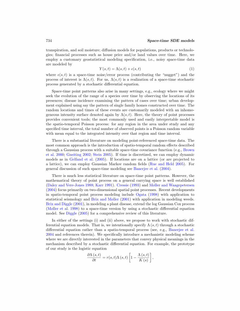
In Figure 8 we display the posterior mean intensity surface for year 1966 and thepredictive mean intensity surfaces for years 1967, 1968 and 1969. We also overlay theactual point patterns of the new homes construct in those four years on the intensitysurfaces. Figure 8 shows that our model can forecast the major areas of high intensity,hence high growth very well. For example, in the upper left corner, the intensity contin-ues rising from 1966 to 1968 and starts to wane in 1969. We can see increasing numbersof houses are built from 1966 to 1968 and much fewer are built in 1969. In the lowerleft part of the plots near the bottom, we can see areas of high intensity gradually shiftdown to the south and the house construction pattern confirms this trend too.

5 Discussion

We have illustrated the use of stochastic differential equations to model both geostatis-tical and point pattern space-time data. Our examples demonstrate that the proposedhierarchical modeling can accommodate the complicated model structure and achievegood estimation and prediction. The major challenges in fitting our proposed modelsare: (i) the evaluation of a likelihood that involves discretization of the SDE in time andstochastic integrals and (ii) a likelihood that does not allow an easy formulation of an ef-ficient Metropolis-Hastings algorithm. In dealing with the first challenge, we utilize theEuler approximation and the space discretization method in Benes et al. (2002). Thoughthe simulation results are encouraging, further investigation of these approximations or

3The growth curves for the house construction data are much smoother than those in our simulateddata example in Section 3.3. Although our fitted mean growth curves seem to match the data tooperfectly, we do not think we overfit because our hold-out prediction results are very accurate as well.


alternatives would be of interest. For the second, we apply the random-walk Metropolisalgorithm to the posterior simulation, which is liable to create large auto-correlation inthe sampling chain. The nonlinear and recursive structure of our likelihood makes mostof the current Metropolis methods inapplicable, encouraging future research for a moreefficient Metropolis-Hastings algorithm for this class of problems.

Our application to the house construction data is really only a first attempt toincorporate a structured growth model into a spatio-temporal point process to affordinsight into the mechanism of urban development. However, if it is plausible to assumethat the damping effect of growth is controlled by the carrying capacity of a logisticmodel, then it is not unreasonable to assume the growth rate is mean-reverting. Ofcourse, we can envision several ways to make the model more realistic and these suggestdirections for future work. We might have additional information at the locations toenable a so-called marked point process. For instance, we might assign the house to agroup according to its size. Fitting the resultant multivariate Cox process can clarifythe intensity of development. We could also have useful covariate information on zoningor introduction of roads which could be incorporated into the modeling for the rates.We can expect “holes” in the region - parks, lakes, etc. - where no construction canoccur. For locations in these regions, we should impose zero growth. Finally, it may bethat growth triggers more growth so that so-called self exciting process specificationsmight be worth exploring.

ReferencesBanerjee, S., Carlin, B., and Gelfand, A. (2004). Hierarchical Modeling and Analysis

for Spatial Data. Chapman & Hall/CRC. 734

Benes, V., Bodlak, K., Møller, J., and Waagepetersen, R. (2002). “Bayesian Analysisof Log Gaussian Cox Processes for Disease Mapping.” Technical Report R-02-2001,Department of Mathematical Sciences, Aalborg University. 746

Brix, A. and Diggle, P. (2001). “Spatiotemporal prediction for log-Gaussian Cox pro-cesses.” Journal of the Royal Statistical Society: Series B, 63: 823–841. 734, 737,743

Brix, A. and Møller, J. (2001). “Space-time multi type log Gaussian Cox Processes witha View to Modelling Weeds.” Scandinavian Journal of Statistics, 28: 471–488. 734

Brown, P., Karesen, K., Roberts, G., and Tonellato, S. (2000). “Blur-generated non-separable space-time models.” Journal of the Royal Statistical Society: Series B, 62:847–860. 734, 738

Cressie, N. (1993). Statistics for Spatial Data. New York: Wiley, 2nd edition. 734

Daley, D. and Vere-Jones, D. (1988). Introduction to the Theory of Point Processes.New York: Springer Verlag. 734


Diggle, P. (2005). “Spatio-temporal point processes: methods and applications.” Dept.of Biostatistics Working Paper 78, Johns Hopkins University. 734

Elerian, O., Chib, S., and Shephard, N. (2001). “Likelihood inference for discretelyobserved non-linear diffusions.” Econometrica, 69: 959–993. 735, 736

Gelfand, A. E., Banerjee, S., and Gamerman, D. (2005). “Spatial process modellingfor univariate and multivariate dynamic spatial data.” Environmetrics, 16: 465–479.734

Gneiting, T. (2002). “Nonseparable, stationary covariance functions for space-timedata.” Journal of the American Statistical Association, 97: 590–600. 734

Golightly, A. and Wilkinson, D. (2008). “Bayesian inference for nonlinear multivariatediffusion models observed with error.” Computational Statistics and Data Analysis,52: 1674–1693. 736

Jones, R. and Zhang, Y. (1997). “Models for continuous stationary space-time pro-cesses.” In Gregoire, G., Brillinger, D., Diggle, P., Russek-Cohen, E., Warren, W.,and Wolfinge, R. (eds.), Modelling Longitudinal and Spatially Correlated Data, 289–298. Springer, New York. 738

Karr, A. (1991). Point Processes and Their Statistical Inference. New York: MarcelDekker, 2nd edition. 734

Kloeden, P. and Platen, E. (1992). Numerical Solution of Stochastic Differential Equa-tions. Springer. 735, 738

Kot, M. (2001). Elements of Mathematical Ecology . Cambridge Press. 735

Mahajan, V. and Wind, Y. (1986). Innovation Diffusion Models of New Product Ac-ceptance. Harper Business. 735

Møller, J., Syversveen, A., and Waagepetersen, R. (1998). “Log Gaussian Cox pro-cesses.” Scandanavian Journal of Statistics, 25: 451–482. 734

Møller, J. and Waagepetersen, R. (2004). Statistical Inference and Simulation for SpatialPoint Processes. Chapman and Hall/CRC Press. 734

Ogata, Y. (1998). “Space-time point-process models for earthquake occurrences.” An-nals of the Institute for Statistical Mathematics, 50: 379–402. 734

Rue, H. and Held, L. (2005). Gaussian Markov random fields: theory and applications.Chapman & Hall/CRC. 734

Stein, M. L. (2005). “Space-time covariance functions.” Journal of the American Sta-tistical Association, 100: 310–321. 734

Stramer, O. and Roberts, G. (2007). “On Bayesian analysis of nonlinear continuous-timeautoregression models.” Journal of Time Series Analysis, 28: 744–762. 736


Whittle, P. (1963). “Stochastic processes in several dimensions.” Bulletin of the Inter-national Statistical Institute, 40: 974–994. 738

Zhang, H. (2004). “Inconsistent estimation and asymptotically equal interpolationsin model-based geostatistics.” Journal of the American Statistical Association, 99:250–261. 741, 745

Acknowledgments

The authors thank Thomas Thibodeau for providing the Dallas house construction data.


0 2 4 6 8 10

02

46

810

Longitude

Latitu

de

1

2

3

4

A

B

C

D

Figure 1: Locations for the simulated data example in Section 3.3.



0 5 10 15 20 25 30

0.0

0.2

0.4

0.6

0.8

1.0

Timeline

Lo

ca

tio

n 1

0 5 10 15 20 25 30

0.0

0.2

0.4

0.6

0.8

1.0

Timeline

Lo

ca

tio

n 2

0 5 10 15 20 25 30

0.0

0.2

0.4

0.6

0.8

1.0

Timeline

Lo

ca

tio

n 3

0 5 10 15 20 25 30

0.0

0.2

0.4

0.6

0.8

1.0

Timeline

Lo

ca

tio

n 4

Figure 2: Observed space-time geostatistical data at 4 locations, actual (dashed line) andfitted mean growth curves (solid line), and 95% predictive intervals (dotted line) by our model(12) for the simulated data example.


0 5 10 15 20 25 30

0.0

0.2

0.4

0.6

0.8

1.0

Timeline

Ne

w L

ocatio

n A

0 5 10 15 20 25 30

0.0

0.2

0.4

0.6

0.8

1.0

Timeline

Ne

w L

ocatio

n B

0 5 10 15 20 25 30

0.0

0.2

0.4

0.6

0.8

1.0

Timeline

Ne

w L

oca

tio

n C

0 5 10 15 20 25 30

0.0

0.2

0.4

0.6

0.8

1.0

Timeline

Ne

w L

oca

tio

n D

Figure 3: Hold-out space-time geostatistical data at 4 locations, actual (dashed line) andpredicted mean growth curves (solid line) and 95% predictive intervals (dotted line) by ourmodel (12) for the simulated data example.


0 5 10 15 20 25 30

−0

.20

.00

.20

.40

.60

.81

.0

Timeline

Ne

w L

oca

tio

n A

0 5 10 15 20 25 30

−0

.20

.00

.20

.40

.60

.81

.0

Timeline

Ne

w L

oca

tio

n B

0 5 10 15 20 25 30

−0

.20

.00

.20

.40

.60

.81

.0

Timeline

Ne

w L

oca

tio

n C

0 5 10 15 20 25 30

−0

.20

.00

.20

.40

.60

.81

.0

Timeline

Ne

w L

oca

tio

n D

Figure 4: Hold-out space-time geostatistical data at 4 locations, actual (dashed line) andpredicted mean growth curves (solid line) and 95% predictive intervals (dotted line) by thebenchmark model (16) for the simulated data example.


Figure 5: Growth of residential houses in Irving, TX.


Figure 6: The gridded study region encompassing Irving, TX.


5 10 15

01

00

20

03

00

40

0

Year

Nu

mb

er

of

Ho

use

s

Block 1

5 10 15

01

00

20

03

00

40

0

Year

Nu

mb

er

of

Ho

use

s

Block 2

5 10 15

01

00

20

03

00

40

0

Year

Nu

mb

er

of

Ho

use

s

Block 3

5 10 15

01

00

20

03

00

40

0

Year

Nu

mb

er

of

Ho

use

s

Block 4

Figure 7: Mean growth curves (solid line) and their corresponding 95% predictive intervals(dotted lines) for the intensity for the four blocks marked in Figure 6.


Figure 8: Posterior and predictive mean intensity surfaces for the years 1966, 1967, 1968 and1969

Documents

Modeling space-time data using stochastic diﬁerential