Embed Size (px)
Citation preview

1
Sixth Triennial Symposium on Transportation Analysis Phuket Island, Thailand, 10-15 June 2007
Modeling Residential and Spatial Search Behaviour: Evidence
from the Greater Toronto Area
Muhammad Ahsanul Habib
(Corresponding author)
PhD Candidate, Department of Civil Engineering
University of Toronto, 35 St. George Street, Toronto, ON, M5S 1N1
Phone: 416-9785049, Fax: 416-9785054
Email: [email protected]
Eric J. Miller
Bahen-Tanenbaum Professor, Department of Civil Engineering
University of Toronto, 35 St. George Street, Toronto, ON, M5S 1N1
Phone: 416-9784076, Fax: 416-9785054
Email: [email protected]
Abstract
This papers attempts to conceptualize the residential mobility and spatial search process
as a part of comprehensive Residential Mobility and Location Choice (REMLOC) model
to be implemented within a microsimulation-based integrated modeling framework and
presents empirical results of household mobility-decision models using Greater Toronto
Area (GTA) retrospective survey data. In implementing mobility models, both discrete
choice and hazard-based duration models are tested in order to aid time- and event-driven
microsimulation respectively. Within discrete choice framework, binomial choice panel
logit models are examined that include fixed effects, random intercept and random
parameter models. On the other hand, parametric hazard duration models are investigated
with various assumptions concerning the baseline distribution. In addition, the paper
investigates frailty models that account for unobserved heterogeneity for both univariate

2
and multivariate hazard models. While the Random Parameter (RP) model performs
better in identifying residential stressors that lead to mobility, the log-logistic Gaussian
shared frailty model shows promising results in explaining termination of passive-state
duration. The study reveals that most stressors that relate to life cycle events such as job
change, birth of a child, increase/decrease in number of jobs etc. are significant in the RP
Model. On the other hand, dwelling and neighbourhood characteristics are dominant in
the continuous-time shared frailty model. The estimation results of both techniques give
important behavioural insights and better understanding of residential mobility processes,
which can be incorporated in the microsimulation-based integrated urban models.
Keywords: mobility and search, binomial logit, random parameter, hazard model, frailty
1. Introduction
Since residential mobility and location choice is an important part of integrated land use
and transportation models to understand relationships between transportation and land
uses, it is necessary to explicitly model the “decision-making process” of relocation
incorporating its underlying behaviour. This paper presents a comprehensive conceptual
model of residential mobility and location choice (REMLOC) and identifies various
decision components starting from the decision to become active in the housing market
through spatial search of dwellings that ends up with bidding process to secure a new
location. It also implements households’ mobility decision component by using two
different techniques: discrete choice and hazard-based duration modeling. Understanding
the mobility process is very important to identify behavioural responses due to changes
within the households and their surroundings, which will provide tools to test various
public policies and link with the residential location choice processes that has significant
influence on the composition of neighbourhoods, travel patterns and commuting. One of
the significant contributions of this paper is that it extends standard binomial choice
models of residential mobility explicitly recognizing panel effects. With the retrospective
survey data three different specifications, fixed effects, random intercept and random
parameter models are investigated to incorporate unobserved heterogeneity due to panel

3
structure. To our knowledge, the empirical application of Random Parameter (RP) model
in analyzing residential mobility in this paper is unique in literature. On the other hand,
hazard-based duration models are examined to recognize dynamics of duration in taking
mobility decisions. In other words, these models attempt to test likelihood of termination
of passive-state duration depending upon the length of time spent from the beginning of
the event (being active in the housing market) as well as other related covariates.
The paper is organized as follows: the next section discusses a comprehensive residential
mobility and spatial search process to be implemented within REMLOC. Section 3
provides concepts and estimation procedures of the techniques applied to model
residential mobility. Section 4 briefly describes the data used for the empirical
application. Section 5 discusses results of both binary choice panel logit and hazard-
based duration models. Finally, Section 6 concludes with a summary of contribution of
this study and future research directions.
2. Conceptual framework: Mobility and Spatial Search
Assuming a sequential decision making process (see discussions in Habib and Miller,
2005, 2007) the Residential Mobility and Location Choice (REMLOC) Model consists of
three interrelated components: Mobility decisions, Spatial search and Bidding process to
secure alternative locations. In this section the conceptual framework of each of these
modeling components are briefly discussed.
The residential mobility component determines for each decision making unit (DMU) the
decision to search for dwellings and the timing of mobility decisions. It is hypothesized
that DMUs take these decisions for adjustments with housing needs based on stressors
arising from changes in household composition and different life cycle events as well as
surrounding environments (for recent literature reviews see Habib and Miller, 2007;
Clark and Ledwith, 2005). Since DMUs could act differently in response to stressors (for
example in case of job change one could either buy a new car to reduce burden of
commuting or change dwelling), a stress management component is introduced to deal

4
with stress-release mechanism. Once a DMU take a decision to search, it enters into the
spatial search process, which is a very complex process involving an array of decisions to
make before the bidding for selected alternative dwellings to relocate. Figure 1 details a
conceptual framework to model spatial search.
At first, it is assumed that every DMU has a mental perception how to search. It has
certain objectives. Either they are a “forced mover” due to occurrence of any major
triggering event (such as in-migration, formation of new household through marriage or
separation) or “choice movers” under a certain level of stress (for example, room-stress
due to birth of a new child, commuting stress due to change in job etc). As such, DMUs
know what they need (at least a crude estimate). This mental model would be tried to
capture by “(Selection of) search strategies” component. That means the outputs of stress
and stress-release mechanism will guide the formulation of strategies. In addition, socio-
economic characteristics might have impact on selecting strategies.
Of course, there are arguments that DMUs might have some advance knowledge of the
market through day-to-day activities like reading newspapers, driving through a
neighborhood and seeing rental advertisements. These phenomena arguably also have
impacts on selecting strategies. But they are not sufficient condition for considering a
move and deliberately searching dwellings to improve existing utility of residential
location. So this model would use this “past knowledge and experience” as one of the
factors in shaping strategies, but the process will be dealt with a separate component
(“passive information”) and placed within the “information channel” component.
In reality, search strategies could be of numerous kinds. For simplicity, this conceptual
model would preliminary focused on following strategies:
� Anchor-based search (anchor at current job and/or residence),
� Supply-driven search, area-based sequential search,
� Area-based simultaneous search and
� Learning-based search (see Huff, 1986; Pushkar, 1998).

5
The key outcome of the “strategy of search” component is that it will give a big sample
of dwelling units that are available in the market in a given period of time for a particular
DMU. However, a searcher, in reality, does not know this choice set. But, from the
modeling perspective, inference on strategic choice has a great impact. Having sub-
sample of alternatives (even if it is big) from the citywide set (which will be exogenously
determined) would be very helpful. However, the actor who is searching will not be given
this information (only the model would know it). Rather, a filtered set of choice will be
passed to the actor, which will be produced from the level of information it might gain
through active or passive search (and also from social networks).
As such, the “information channel” is very important part of search stage. In reality,
information search activities can take a variety of forms: first, relying on Internet search
(predominantly, for renters, thanks to IT technologies), attending open houses, searching
commercial advertisements, contacting real estate agents, reviewing advertisement,
calling developers etc. It would also include physically visiting a neighborhood to see
“For Rent” or “For Sale” signs on poles or front yards. In addition, a DMU could be
informed by friends, relatives, neighbors, colleagues and other “alters” of his/her social
network.
The information a searcher could gain from these channels would actually filter the “big
choice set” (obtained from previous component) and would help creating “awareness
space” (i.e. a set of dwelling units that an actor knows for certain they physically exist).
For this set of dwellings a searcher can somehow assign “place utilities”. However, it is
assumed that the DMU will not visit each of these dwellings, even may not extensively
search more information on all of those that requires defining “search space” which is a
sub-set of “awareness space”. The argument is that the filtered information might
produce some useless options that do not match the “mental aspiration region” of a
person seeking a dwelling. Mental aspiration regions reflect an upper-limit and lower-
limit that the DMU has in mind about the attributes of the dwelling (in terms of
structural, neighborhood, even transport options). For example, some people seek to rent

6
only one-bedroom apartment, and some “captive transit riders” have a minimum and
maximum walking distance from the residence in mind. To capture these limits, this
“mental aspiration region” is proposed, which will further screen out the “choice set”
while taking actual decisions during search.
Until now, the searchers actually do not take any real decision other than collecting
information and processing in response to mental simulations. The main decision
components during search are: (a) Final screening of dwelling units from the “choice set”
obtained from “search space” and matching with “mental aspiration region”, (b) Defining
prospect set (a set of dwelling that would be physically visited (i.e. “vacancy visit”) to
see and understand the value and utility of owning/renting), (c) Evaluation of selected
dwellings in the prospect set (d) Defining bidding set after vacancy visit and evaluation.
Once a DMU decides on alternative dwellings on which to bid, a bid formation,
negotiation and acceptance/rejection process would take place within which both buyers
and sellers interact.
Although the entire REMLOC model as outlined in the Figure 1 considers a sequential
process involving mobility, search, and bid, it is expected that once each component is
individually modeled potential feedbacks could be introduced to make the model more
realistic and behaviourally sound. It is expected that it will be possible to operationalize
this conceptual model of relocation with two retrospective surveys, the Residential
Mobility Survey (RMS II 1998) and Residential Search Survey (RSS 1998) conducted for
the Greater Toronto Area, and some additional survey needed in the near future.
However, this paper attempts only to model the first component of decision to search
using RMS II 1998 data for a sample of 270 GTA households that contains housing
career, employment history and household composition changes for a period of 1971-
1998. In the following section model structures of the mobility component are briefly
discussed.

7
3. Model structures for empirical application
For mobility, a DMU first decides whether to become active in the housing market at a
given point of time or not. Two different modeling techniques are applied for the
purpose: discrete choice methods and hazard-based duration models.
3.1 Discrete choice models
Within discrete choice framework, binomial logit panel data models are investigated with
different assumptions on the heterogeneity structures that include Fixed Effects (FE),
Random Intercept (RI) and Random Parameter (RP) models.
The FE model specification is used to accommodate individual heterogeneity in the panel
models by examining group specific effects:
)()1( itiit xgyP βα ′+== (1)
where )1( =ityP represents probability of binary choice of being active in the housing
market and iα denotes group specific effects. In this particular application, a group
means a DMU that has sequence of choice occasions over time. For a given set of DMUs
),.....2,1( ni = at different unit time periods (i.e. choice occasions, ),.....2,1( iTt = the
unconditional log-likelihood function is given by:
∑ ∏= =
′+−Λ=
n
i
T
t
itiit
i
xyLogL1 1
)])(12[(log βα (2)
where Λ is the CDF of logistic distribution. The conditional log-likelihood can be
obtained by conditioning the contribution of each group on the sum of the observed
outcome, which can then be maximized with respect to the slope parameters without
estimating fixed effects parameters (see Chamberlain, 1980). However, direct
maximization of the log-likelihood function with all parameters is possible by brute force
maximization taking advantage of the properties of the sparse second derivatives matrix
(see Greene, 2001 for details).

8
While the parameter vector iβ has a fixed component and a sub-vector that varies across
groups in the FE models, it is constant across groups and periods for the Random
Intercept (RI) models. But the later type has a time invariant component, which is the
latent heterogeneity that enters into the model in the form of random effects:
)()1( iitit xgyP ψβ +′== (3)
where iψ is the unobserved heterogeneity same in every period.
On the other hand, in the Random Parameters (RP) model, all the parameters can vary
randomly over individuals. The structure of the model is based on the conditional
probability:
Prob [ ] iitiiitit TtNixgxy ,.......1,,......,1),(1 , ==′== ββ (4)
The model is operationalized by writing: iii vz Γ+∆+= ββ (5)
where iz is a set of M observed variables which do not vary over time and enter into the
means of the random parameters. ∆ represents a coefficient matrix that forms the
observation-specific term in the mean. And Σ is the diagonal matrix of scale parameters
(i.e. standard deviations). The random vector iv induces the random variations in the
reduced form parameters of the model. The unconditional likelihood function is given by
∫∏ =′=Φ
i
i
v
ii
T
t itriitiiii dvvfxygzxyL )(),(),,|(1 ,β (6)
Since this likelihood function is a multivariate integral that cannot be evaluated in closed
form, the parameters are estimated by simulation (See Train, 2003). The simulated log-
likelihood function is
∑ ∑ ∏= = =′=
N
i
R
r
T
t itriits
i
xygR
LogL1 1 1 , ),(
1log β (7)
The simulation is carried out over R draws on riv , through ri ,β . The maximum simulated
likelihood estimator is obtained by maximizing equation (7) over the full set of structural
parameters Φ . Eventually estimates of structural parameters and their asymptotic
standard errors are generated from this simulated maximization procedure (see Greene,
2004, and Train, 2003 for details).

9
In the RP Model it is needed to assume specific distributions for random parameters. In
most applications such as Revelt and Train (1998), Mehndiratta (1996), and Ben-Akiva
and Bolduc (1996) it has been specified to be normal or lognormal. On the other hand,
Revelt and Train (2000), Hensher and Greene (2001), and Train (2001) have used
triangular and uniform distributions. This paper assumes all random parameters to be
normally distributed with zero mean and unknown variance. In practice, it is often found
that some of the parameters are random while others are nonrandom. In such cases,
nonrandom parameters in the model are implemented by constraining corresponding rows
in ∆ and lower triangular matrix to be zero. Note that in the Random Intercept (RI) model
only the constant term is assumed to be random while all other parameters are
nonrandom. In other words, the RI model can be seen as the RP model in which only the
constant term is random.
3.2 Hazard-based duration models
In addition to discrete choice models, this paper investigates continuous time hazard-
based duration models to analyze mobility decisions. Hazard-based duration model
recognizes dynamics of duration since likelihood of termination of duration depends on
the length of time spent from the beginning of an event. It has wide applications in the
fields of engineering, medical sciences and labour force analysis and the basic principles
are well discussed in Kalbfleisch and Prentice (2002), Lancaster (1990) and Hougaard
(2000). For a housing market application, let T be a continuous, non-negative valued
random variable representing time until active in the housing market of a Decision
Making Unit (DMU). If the probability of a DMU leaving the passive-state within a short
interval t∆ at or after t is )|( tTttTtP ≥∆+<≤ while the DMU is still passive in the
market at t, then the hazard rate can be obtained simply dividing the probability by t∆
that represents average probability of leaving the state per unit of time. Considering this
average over very short intervals the hazard function )(tλ , which is the instantaneous rate
of failure at t, is given by
t
tTttTtPt
t ∆
≥∆+<≤=
→∆
)|(lim)(
0λ (8)

10
This basic formulation of hazard function allows relating it with probability density
function )(tf , cumulative distribution function )()( tTPtF ≤= and survival function
)(1)()( tFtTPtS −=≥= . Since the probability density function of T is
dt
tdS
dt
tdF
t
ttTtPtf
t
)()()(lim)(
0
−==
∆
∆+<≤=
→∆, the hazard function can be written as
dt
tSd
tS
tf
tF
tft
)(log
)(
)(
)(1
)()(
−==
−=λ (9)
Since we are interested in investigating factors affecting termination of duration this non-
parametric model is extended to incorporate explanatory variables (in the form of
covariates) leading to semi-parametric and parametric models. Semi-parametric models
assume hazard rate to be proportional and baseline hazard to be parametrically
unspecified. The most popular proportional model exploits partial likelihood estimation
techniques put forwarded by Cox (1972) and takes the following form:
))(exp()(),( 0 txtxt λλ = (10)
where x(t) is the vector of observed covariates and )(0 tλ is the baseline hazard which is
not parametrically specified. But parametric models assume a distribution for the baseline
hazard and hence for the survival function. In many cases knowledge of the baseline
hazard is unnecessary, for example, in comparing control and treatment groups for
mortality due to a specific disease while applying a new drug. However, like many other
instances tackled by event history researchers, in microsimulating urban systems, it is
useful to have clear inference about )(0 tλ since such a modeling framework requires
identification of timing of entry and exit in the housing market, labour force and school
etc. Although it is possible to retrieve baseline hazards in semi-parametric models (for
details see Box-Steffensmeier and Jones, 2004, Kalbfleisch and Prentice, 2002 and
Collett, 1994 among others) this study prefers parametric models since they provide
direct inference on the duration dependence. In addition, this paper makes an accelerated
failure time (AFT) assumption (i.e. the covariates directly rescale time), which can be
expressed as a log-linear model:

11
σεβ +′= xT j)log( (11)
where jβ are the coefficients of the time independent covariates x and ε is a stochastic
error term with type-I extreme value distribution scaled by σ . The hazard function of
the AFT models is given by
)()(
0 exp)exp(),( xxtxt
ββλλ −−= (12)
Here the effect of covariates is to alter the rate at which a person proceeds through time
by either accelerating or decelerating the termination of duration.
There are wide varieties of distributions that can be employed in the parametric models
including exponential, Weibull, log-logistic, log-normal, gamma, generalized F,
Gompertz, Makeham etc. (for detail discussion on each distribution see Lancaster, 1990;
Kalbfleisch and Prentice, 2002; Deshpande and Purohit, 2006). This paper tested
Weibull, log-logistic and exponential distributions. While the exponential distribution has
the no-ageing phenomenon due to lack-of-memory property, the Weibull distribution is a
generalization of exponential distribution that provides constant, strictly increasing (or
decreasing) hazard functions. Hence the hazard rate for Weibull distribution can be
expresses as
1)()( −= ptpt ϕϕλ (13)
where ϕ is a positive scale parameter and p is known as the shape parameter. When
1>p , the hazard rate increases as t increases from 0 to ∝. In other words, there is a
positive duration dependence (i.e. positive ageing, also called “snowballing effect”)
which means that the longer the elapsed duration the unit is more likely to exit soon. On
the other hand, if 10 << p then the hazard decreases with time (i.e. negative ageing, also
called “inertia effect”). In case of 1=p it becomes exponential with mean ϕ/1 and if
2=p it becomes Rayleigh distribution for which hazard rate is a straight line passing
through the origin with slope ϕ2 . Hence, Weibull models can accommodate both
increasing failure rate (IFR) and decreasing failure rate (DFR) probability distributions
depending upon the free shape parameter p .

12
The paper also considers log-logistic distribution that permits non-monotonic hazard
form in contrast to monotonic Weibull models. The hazard function of the log-logistic
distribution can be written as
))(1/()()( 1 pp ttpt ϕϕϕλ += − (14)
In this case, the hazard decreases monotonically from ∝ at the origin to zero provided
that 1<p and decreases monotonically from p provided that 1=p as t approaches to ∝.
On the other hand, if 1>p , the hazard gets a non-monotonic shape increasing from 0 to a
maximum of )/))1((( /1 ϕppt −= , and decreasing thereafter as t approaches to ∝.
The parameters of the parametric hazard models are estimated using full information
maximum likelihood estimation method (see Kalbfleisch and Prentice, 2002). Since our
data is right Type-I censored, denoting iδ as the censoring indicator (taking the value 0 if
case i is censored and the value 1 if case i experienced the event), the likelihood
function is given by
( ) ( ) )],([],[)],([],[1
ii
n
i
iiii
n
i
ii xtSxtxtSxtfL iii δδδ λ∏∏ == − (15)
This univariate formulation is adequate for analyzing single-spell residential mobility
(see an application in Vlist et al., 2001). However, this study is using retrospective data
that has repeated events recorded for each DMU. Failure to account for this repeatability
might violate independence assumption on the occurrence of events taken in single-spell
models. Two general approaches are applied in such cases: variance-corrected approach
and random effects/frailty approaches (for extensive review see Box-Steffensmeir, 2004
and Hougaard, 2000). While variance-corrected approach estimate a model and then fix
up the variance to account for the fact that the observations are not independent (rather
repeated and therefore correlated), the shared frailty models assumes a stochastic
variation across the parameters that is shared (common) among individuals. This paper
investigates shared frailty models with different assumptions on frailty distributions. If
decision making unit (DMU) i has multiple episodes j , the hazard rate for the j th
episode of the i th DMU can be expressed as
iijiijij vxtxtt )exp()()exp()()( 00 βλωψβλλ ′=′+′= (16)

13
where )exp( iiv ωψ ′= represents group-specific heterogeneity (i.e. shared frailty) that is
distributed across groups (in this case DMUs with repeated episodes) according to some
distribution function )( ivG . Consequently, the likelihood function is given by
( ) )()],([],[1
01
i
g
i
ijij
n
j
ijij vdGxtSxtL ij
i
∏ ∫ ∏=
∞
=
=
δλ (17)
This likelihood function is maximized in order to obtain parameter estimates. The
likelihood ratio test is used to assess the need for inclusion of the frailty component .iv
For both single-episode and repeated events models goodness-of-fit statistics are obtained
by estimating Rho-square, which is one minus the ratio of log-likelihood of the full
model and null model (i.e. constant only model).
4. Data preparation
As discussed earlier this paper uses the RMS II retrospective survey data for a random
sample of 270 GTA households. Detail description of the data can be found in Habib and
Miller (2007). For the discrete choice models, 28 years of longitudinal data (for a period
of 1971-1998) has been extracted from the database that contains yearly observations of
whether decision making units are active in the market or not. It also contains
information on employment history, household composition changes as well as socio-
economic characteristics of the households. Key residential stressors are identified for
each observation year by comparing states between the consecutive years (for example,
job increase/decrease, DMU size increase/decrease etc.). Indicators of lags and leads of
these stressor events are also identified to test in the models. Additional explanatory
variables are generated from census tabulations of the corresponding years. In total, 4097
observations are used for modeling in which DMUs were active in the housing market at
408 choice occasions in different years between 1971 and 1998. Note that the event
“active” in the housing market includes actual moves as well as instances in which the
DMU became ‘active’ in the market but did not end up moving. This ‘active but did not
move’ information is unique in the literature and provides an unbiased database for
14
mobility model development. That is, most data sets only include successful moves and
so underestimate mobility participation rates.
On the other hand, for continuous time hazard-based duration models the same dataset is
selected where 270 households have 623 episodes (that represents passive-state duration
of DMU) including censoring spells. The data is right-censored in the year of 1998. Note
that these duration spells are the continuous time-period within which DMUs are in
passive-state. The state terminates by the occurrence of the event decision-to-move that
triggers actively searching the housing market for potential alternative dwellings. The
average observed duration is 2.3 years with a minimum one year and maximum seven
years. Covariates used for hazard models are also taken from the same sources, but only
those that are constant or assumed to be constant for the entire duration of an episode.
Time varying covariates are not tested in this paper. As such, year of birth of the DMU
head, number of bedrooms and other structural attributes of the dwellings, and
neighbourhood attributes are employed in the models. It also tests whether the first spell
since household formation as well as immigration affects termination of passive-state
duration or not.
5. Discussion of results
5.1 Panel logit models
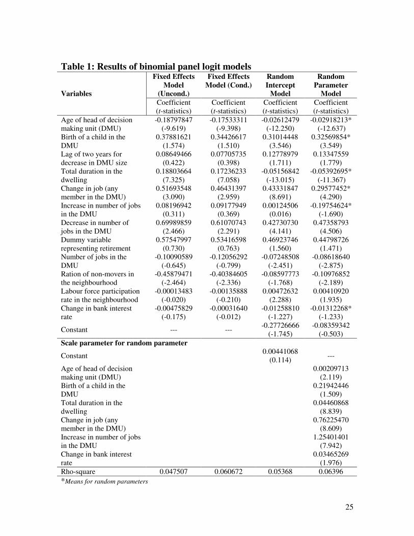
Table 1 reports results of binomial panel logit models described in Section 3.1. Fixed
effects (FE) model estimated through brute force maximization gives similar results as of
the conditional FE model put forwarded by Chamberlain (1980) where fixed effects
parameters are not estimated. In fact, conditional maximum likelihood estimation is
carried out due to presence of incidental problem (i.e. if there is same choice throughout
the observation period). The results shows that incidental problem is not acute for the
sample used for this study and fixed effects models can be estimated using direct
maximization (proposed by Greene, 2001) where all the group-specific effects are
estimated along with coefficients of explanatory variables at the same time. However,
Random Intercept (RI) model shows greater value of good-ness-of fit statistics (i.e. Rho-

15
square) than that of FE models. In the RI model we have a time invariant constant term,
which captures unobserved heterogeneity across decision making units (DMU). But the
highest goodness-of-fit statistics is achieved in the Random Parameter (RP) Model that
captures heterogeneity across the parameters. Hence this paper selected the RP model as
the final model. Description of parameter estimates of the final RP model is given below.
It is found that most of the hypothesized residential stressors (such as increase/decrease
in number of jobs, birth of a child, job change, decrease in DMU size, retirements etc.)
are found to be significant in explaining residential mobility. The fifth column of Table 1
reports mean and standard deviation of the parameters estimated for the RP model. It can
be seen that mostly dynamic variables are found to be random parameters whereas all of
the static variables are nonrandom.
Age of the household head (often used as a proxy variable to mark stages of life cycle,
see Clark et al., 1986, Mulder, 1993, Vlist et al., 2001 among others) have significant
effect on the decision to move. It shows that younger-head DMUs are more frequent
movers than older heads. However, there is some variability of the effect as seen in the
significant standard deviations. Another significant life-cycle event, birth of children also
induces mobility. Similarly, job change increases the probability of moving where the
mean of the parameter is 0.296 with a standard deviation of 0.76. This means that
although change of job location on average significantly encourages a relocation decision
in order to relieve commuting stress, this effect varies considerably across households,
with certain DMUs preferring other stress-release mechanisms (possibly, such as buying
a new car) and do not become active in the housing market in response to this stressor.
While decrease in number of jobs in the DMU increases the probability of moving, a
dummy variable reflecting retirements doubles this effect. Interestingly, these stressors
are found to be non-random across the sample households. However, increase in jobs
shows a very interesting behaviour having negative sign in the parameter value. Our prior
hypothesis was that such an increase would increase the probability of becoming active in

16
the housing market. But the model result suggests an opposite effect. This could partly be
explained by the results of the static variable number of jobs in the household, which is
found to be nonrandom with a coefficient value of – 0.086. That means if there are more
workers in the household, the probability of becoming active is lower, all else being
equal. This presumably reflects inertia effects associated with having more job locations
within which they have already been settled in terms of mode choice, commuting patterns
and other short-term activity agendas. Therefore, an increase in jobs in a DMU actually
brings a similar stationary effect that prevents considering a residential relocation.
However, the parameter of this variable also exhibits a very high variability among the
decision makers having a standard deviation of 1.254 compared to the mean of – 0.198.
This suggests that in some cases an increase in jobs actually does increase the probability
of moving.
Duration at the current home is also found to be one of the significant determinants of
mobility decision. The higher the duration in the current location, the lower the
probability of moving. It proves the hypothesis of inertia that impedes relocation due to
strong community linkages created by longer durations of living in a neighborhood. It is
very much consistent with many other previous findings (such as McHugh et al., 1990).
This study also tried to capture duration effects at different time scales using dummy
variables (such as the first three years in the GTA, three to five years, more than five
years, etc. as well as other alternative combinations), none of which provides expected
impacts on mobility. Hence, in the final model, only total duration is retained, which is
also found to be a random parameter.
In many cross-sectional studies (as well as in some longitudinal mobility research),
tenure was considered to be an important factor in explaining residential mobility. Often
it was found that renters are more mobile than owners. Again, it was found that highly
educated persons tend to have higher mobility rates compared to less educated workers.
Similarly, household size, dwelling type, number of rooms, number of bedrooms, number
of people per room etc. were found to be contributing factors for mobility (see Vlist et

17
al., 2001 for a recent review). But this research indicates that most of these static
attributes of the dwelling as well as decision makers are not significant when dynamic
variables are taken into account in the mobility model.
It is also found that neither job-residence distance nor distance to CBD is significant in
explaining mobility decisions. Rejection of distance to CBD could be explainable due to
the GTA being a multi-centric metropolitan area (although the Toronto CBD is still a
very important employment, shopping and cultural centre within the region). However,
the study was expecting to see effects of job-residence distance or changes in average
job-residence distance within the mobility decision, but these hypotheses were not
confirmed. One possible reason for this unexpected result might be that the stressor “job
change” already captures some of the effects of change in commuting distances.
Although this research examined three years of lag and lead effects for each of the life
cycle stressors, the only significant lag/lead effect found is a two-year lagged response to
a decrease in DMU size. That is, if the DMU size decreases it take two years to have an
impact on the mobility decision. In other words, the probability of moving increases two
years after a DMU size decrease. This is a plausible response, since it may well take a
household some time to decide to adjust its dwelling size and/or location in response to a
change in household size.
Regarding neighborhood dynamics, the model indicates that if a DMU lives in a stable
community, represented by the fraction of non-movers (in the last five years) in the
neighborhood, it is less likely to consider moving. On the other hand, the neighborhood
labor force participation rate has a positive impact on household mobility. Both of these
variables are found to be non-random. A large set of other neighbourhood attributes has
also been examined (for example, average dwelling value, dwelling density, renter/owner
ratio, percentage of immigrants etc.). None of those variables are found to be statistically
significant.

18
Since housing supply data for a long period was not available for use in this study, it uses
some housing market indicators such as change in mortgage rate, bank interest rate, etc.
to include market dynamics in the model. Although this study finds both mortgage rate
and bank interest rate to be significant, due to obvious correlation issues, only one of
these two variables can be included in the final model. Since mortgage rates can vary for
individual cases and RMS II does not provide any information of mortgage premiums,
and equity or savings, the bank interest rate has retained in the final model. Note that this
interest rate only differs across years, not for individual decision makers. Finally, it is
found that changes in interest rate are negatively related with mobility decisions. The
interpretation is that if interest rates increase, decision making units are less likely to be
active in the market and vice versa. This key market indicator is found to be a random
parameter with a statistically significant standard deviation.
Most of the parameters included in the final model, including means and standard
deviations, are statistically significant at the 95% confidence level or better. One or two
estimates fall short of the corresponding t statistics value (1.64). However, they are
retained in the model due to their importance as policy variables (such as change in
interest rate) in an expectation that with larger sample the variables would be statistically
significant.
5.2 Hazard-based duration models
The first set of hazard-based duration models is estimated assuming single-spell for each
termination. That means, each episode at the passive-state in the market for a given DMU
is assumed to be independent and considered as separate observation in the analysis. But
given the fact that we have collected retrospective data that contains information on the
housing career of each household, it is more appropriate to consider repeated events
models. As discussed earlier although there are different ways of dealing with this
phenomena we estimated shared frailty models where the frailty component accounts for
unobserved heterogeneity that is common for the households that have multiple
sequential episodes. The study also tested frailty models for the single-spell assumption

19
in which frailty only considers individual-level heterogeneity (not group-level as in
shared frailty). Since with the retrospective data we are more interested on the group-
level unmeasured risk factors this paper only reports repeated events shared frailty
models. Three different distribution assumptions are used for frailty in these models
including gamma and inverse Gaussian (see Clayton, 1978 and Hougaard, 2000) and
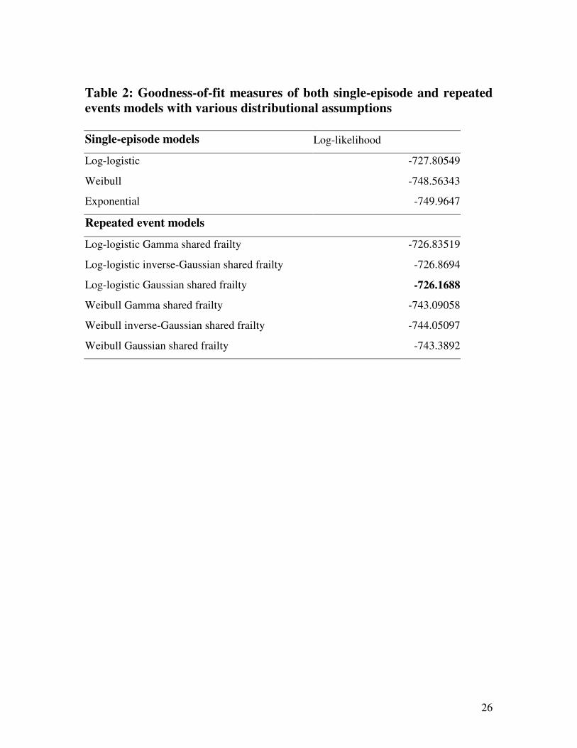
Gaussian distribution (see Greene, 2002). The goodness-of-fit measures for both basic
single-spell models with different assumptions on baseline hazard and repeated events
shared frailty models are tabulated in Table 2. As indicated by the goodness-of-fit
measures, the log-logistic model with Gaussian frailty describes the termination
probability best. While Table 3 presents coefficient estimates of all basic single-episode
models, Table 4 shows some competitive shared frailty models. It can also be seen that
most of the parameter estimates of the log-logistic Gaussian frailty model are statistically
significant at the 95% confidence level in contrast to other candidate models. Since the
log-logistic Gaussian frailty model is selected as the final model its results are detailed
below.
It is found that age of the DMU head (represented by the year of birth) has significant
impact on the passive-state duration. Older DMU head stays passive in the housing
market longer than younger heads. Also, a DMU who has higher number of rooms in the
dwelling unit it lives have longer duration. Similarly, DMUs living in the row houses
have longer duration; possibly under income constraints they are less likely to become
frequently active in the market. Tenure also affects duration; renters are more frequently
active in the market than homeowners. Both higher dwelling density and single-detached
housing density in the neighborhood increases duration of stay. However, impact of
single-detached housing density is higher than that of all dwellings. This reflects that
DMUs that secured housing in a single-detached dominated neighborhood are less likely
to change their dwellings frequently.
While increased share of non-movers in the neighborhood increases duration, share of
immigrants in the neighborhood does the opposite. This means that DMUs living in a
20
stable neighborhood are less likely to consider moving, but those who live in an
immigrant-dominated area are more prone to move. On the other hand, labour force
participation rate in a neighborhood increases duration of being passive in the housing
market.
Distances to Toronto CBD also have impact on duration; people living close to the CBD
are more frequently active in the market than people in suburban areas. It is intuitive that
DMUs living in the suburbia have already obtained a stable location by purchasing
dwellings. Both dummy variables indicating new household formation and new
immigrants in GTA show positive impact on duration. That is, in the first spell since
formation of household and immigration, DMUs tend to stay longer than other spells in
general. However, DMUs forming new households have longer duration than that of
immigrants.
Finally, the value of ancillary parameter ( p ) greater than one suggests that the hazard
initially increases to a certain point and decreases thereafter. The model also shows
considerable variance of the distribution of the random effects (θ ), which is statistically
significant when tested against a Chi-square distribution. That is, the null hypothesis
( 0=θ ) is rejected for the log-logistic shared frailty model.
5.3 Comparison between panel logit and hazard models
It is not possible to directly compare these two modeling techniques examined to explain
residential mobility. The focus of the discrete choice modeling was to see how
households decide at each choice occasion to be active in the market. On the other hand,
hazard-based duration models directly model termination of passive-state duration
resulting the event of being active in the market. Although outcomes of the process
modeled through these two techniques are the same, due to methodological differences
and variable selection makes it hard to directly compare the results of both. In the panel
data logit models, most of the variables selected mark dynamic changes at each unit time
period (i.e. year). On the other hand, the variables that are constant (or assumed to be

21
constant) over the whole duration period are used for the continuous-time hazard models.
Note that time-varying covariates are not tested in this paper. As such, mostly dwelling
attributes and neighbourhood characteristics are found in the hazard models. However,
common variables in both types of models show identical results in explaining mobility.
For instance, younger-heads are more frequently active in the market than older-head
households and higher labour force participation rates in the neighbourhood contribute
larger duration meaning less prone to active in the market. On the other hand, the
variables which are rejected in the panel logit models (such as tenure, dwelling density)
are found significant in the hazard models. Perhaps, in the presence of dynamic variables
these variables do not add explanatory power in the logit models. One interesting finding
has been achieved through continuous-time hazard models is that the first spell of
forming new households and also first spell after immigration lengthen duration of stay
before considering a move to the next. This type of spell-specific characteristics
presumably could only be incorporated in the continuous time hazard models.
6. Conclusion
The paper portrays a comprehensive conceptual framework to model residential mobility
and spatial search, which will provide an excellent guideline to carry forward modeling
residential location choice processes. It also presents empirical results of residential
mobility models that applied two different techniques: discrete choice and hazard-based
duration modeling. In general, both modeling techniques perform well and provide useful
results in understanding residential mobility behaviour. Tests and comparison of different
models within each technique also provide important guidelines to cope with
methodological challenges while working with retrospective data. While Random
Parameter (RP) model shows better performance in incorporating latent heterogeneity for
discrete-time data, shared frailty models are found quite satisfying for continuous-time
settings. In general, both final models show reasonable explanatory powers. Also, their
parameter estimates are mostly statistically significant.

22
In the random parameter model, it is found that residential stressors mostly related to job
and household composition dynamics are significant in explaining DMUs’ desire to
change location at each point of time. Notable stressors are increase and decrease in the
number of jobs, change of job location, retirement, birth of children and a two-year
lagged effect for decrease in DMU size. On the other hand, mostly dwelling and
neighbourhood characteristics are found significant in the continuous-time shared frailty
models in the absence of stressors that vary with time. Hence, the next step of the
research should be testing these models by incorporating time-varying covariates and to
see how the model responds.
The models presented in this paper significantly contribute to the residential mobility
research, particularly in exploring methodologies to deal with panel effects when
considering longitudinal data. In addition, it is expected that while the random parameter
binomial logit model will support time-driven microsimulation of the mobility
component in the Integrated Land Use, Transportation and Environment (ILUTE) project,
the frailty model could be applied in case of event-driven microsimulation.
Acknowledgement
This research was funded by a Major Collaborative Research Initiative (MCRI) grant
from the Social Science and Humanities Research Council (Canada) and by the Transport
Canada Transportation Planning and Modal Integration Initiatives program.
REFERENCES
Ben-Akiva, M. and Bolduc, D. (1996) “Multinomial Probit with a Logit Kernel and a
General Parametric Specification of the Covariance Structure”, Working paper,
Department of Civil and Environmental Engineering, MIT.
Box-Steffensmeier, J.M. and Jones, B.S. (2004) Event History Modeling: A Guide for
Social Sciences, Cambridge University Press
Chamberlain, G. (1980) “Analysis of Covariance with Qualitative Data”, Review of
Economic Studies, 47, pp.225-238

23
Clark, W.A.V. and Ledwith, V. (2005) “Mobility, Housing Stress and Neighborhood
Contexts: Evidence from Los Angeles”, Paper ccpr-004-05, On-Line Working
Paper Series, California Center for Population Research.
[http://repositories.cdlib.org/ccpr/olwp/ccpr-004-05]
Clark, W.A.V., Deurloo M., Dieleman, F. (1986) “Residential Mobility in Dutch Housing
Markets”, Environment and Planning A, 18, pp. 763–788
Clayton, D.B. (1978) “A Model for Association in Bivariate Life Tables and Its
Application in Epidemiological Studies”, Biometrica, 65, pp. 141-151
Collett, D. (1994) Modeling Survival Data in Medical Research, Chapman & Hall,
London
Cox, D.R. (1972) “Regression Models and Life Tables”, Journal of the Royal Statistical
Society, B, 26, pp. 186-220
Deshpande, J.V. and Purohit, S.G. (2006) Life Time Data: Statistical Models and
Methods, World Scientific Publishing Co. Pte. Ltd., Singapore
Greene, W. H. (2001), “Fixed and Random Effects in Nonlinear Models”, Working
Paper, Department of Economics, Stern School of Business, New York University
[http://pages.stern.nyu.edu/~wgreene/]
Greene, W. H. (2002) LIMDEP Version 8.0 Econometric Modeling Guide, Vol. 1&2,
Econometric Software, Inc, Plainview, NY
Greene, W. H. (2004), “Interpreting Estimated Parameters and Measuring Individual
Heterogeneity in Random Coefficient Models”, Working Paper, Department of
Economics, Stern School of Business, New York University
[http://pages.stern.nyu.edu/~wgreene/]
Habib, M.A. and Miller, E.J. (2007) “Microbehavioural Location Choice Process:
Estimation of a Random Parameter Model for Residential Mobility” Proceedings
of the 11th
World Conference on Transportation Research, Forthcoming.
Habib. M.A. and Miller, E.J. (2005) “Dynamic Residential Mobility Decision Choice
Model in the ILUTE Framework”, Presented at the 52nd
North American Meeting
of the Regional Science Association International, Las Vegas, November 10-12
Hensher, D. and Greene, W. (2001) “The Mixed Logit Model: The State of Practice and
Warning for the Unwary”, Working paper, School of Business, The University of
Sydney
Hougaard, P. (2000) Analysis of Multivariate Survival Data, Cambridge University Press

24
Huff, J.O. (1986) “Geographic Regularities in Residential Search Behaviour”, Annals of
the Association of American Geographers, 76, pp. 208-227
Kalbfeisch, J. D. and Prentice, R. L. (2002) The Statistical Analysis of Failure Time
Data, John Wiley & Sons, Chichester, Second Edition
Lancaster, T. (1990) The Econometric Analysis of Transition Data, Cambridge
University Press
McHugh, K, Gober, P. and Reid, N. (1990) “Determinants of Short and Long term
Mobility Expectations for Home Owners and Renters”, Demography, 27, pp. 81-
95
Mehndiratta, S. (1996), “Time-of-day effects in Inter-city Business Travel”, PhD Thesis,
University of California, Barkley
Mulder, C.H. (1993) “Migration Dynamics: A Life Course Approach”, PhD Thesis,
Utrecht University, Utrecht.
Pushkar, A.O. (1998) “Modelling Household Residential Search Processes: Methodology
and Preliminary Results of an Original Survey”, M.A.Sc. Thesis, Department of
Civil Engineering, University of Toronto
Revelt, D. and Train, K. (1998) “Mixed Logit with Repeated Choices: Households’
Choices of Appliance Efficiency Level”, Review of Economics and Statistics, 80,
pp. 1-11
Revelt, D. and Train, K. (2000) “Customer-Specific Taste Parameters and Mixed Logit:
Households’ Choice of Electricity Supplier”, Working Papers E00-274,
Department of Economics, University of California at Berkeley
Train, K. (2001) “A Comparison of Hierarchical Bayes and Maximum Simulated
Likelihood for Mixed Logit”, Working paper, Department of Economics,
University of California, Berkley.
Train, K. (2003) Discrete Choice Methods with Simulation, Cambridge University Press,
Cambridge
Vlist, A.J.V.D., Gorter, C., Nijkamp, P. and Rietveld, P. (2001) “Residential Mobility
and Local Housing Market Differences”, Discussion Paper, Tinbergen Institute
Amsterdam [http://www.tinbergen.nl]
25
Table 1: Results of binomial panel logit models Fixed Effects
Model
(Uncond.)
Fixed Effects
Model (Cond.)
Random
Intercept
Model
Random
Parameter
Model Variables
Coefficient
(t-statistics)
Coefficient
(t-statistics)
Coefficient
(t-statistics)
Coefficient
(t-statistics)
Age of head of decision
making unit (DMU)
-0.18797847
(-9.619)
-0.17533311
(-9.398)
-0.02612479
(-12.250)
-0.02918213*
(-12.637)
Birth of a child in the
DMU
0.37881621
(1.574)
0.34426617
(1.510)
0.31014448
(3.546)
0.32569854*
(3.549)
Lag of two years for
decrease in DMU size
0.08649466
(0.422)
0.07705735
(0.398)
0.12778979
(1.711)
0.13347559
(1.779)
Total duration in the
dwelling
0.18803664
(7.325)
0.17236233
(7.058)
-0.05156842
(-13.015)
-0.05392695*
(-11.367)
Change in job (any
member in the DMU)
0.51693548
(3.090)
0.46431397
(2.959)
0.43331847
(8.691)
0.29577452*
(4.290)
Increase in number of jobs
in the DMU
0.08196942
(0.311)
0.09177949
(0.369)
0.00124506
(0.016)
-0.19754624*
(-1.690)
Decrease in number of
jobs in the DMU
0.69989859
(2.466)
0.61070743
(2.291)
0.42730730
(4.141)
0.47358793
(4.506)
Dummy variable
representing retirement
0.57547997
(0.730)
0.53416598
(0.763)
0.46923746
(1.560)
0.44798726
(1.471)
Number of jobs in the
DMU
-0.10090589
(-0.645)
-0.12056292
(-0.799)
-0.07248508
(-2.451)
-0.08618640
(-2.875)
Ration of non-movers in
the neighbourhood
-0.45879471
(-2.464)
-0.40384605
(-2.336)
-0.08597773
(-1.768)
-0.10976852
(-2.189)
Labour force participation
rate in the neighbourhood
-0.00013483
(-0.020)
-0.00135888
(-0.210)
0.00472632
(2.288)
0.00410920
(1.935)
Change in bank interest
rate
-0.00475829
(-0.175)
-0.00031640
(-0.012)
-0.01258810
(-1.227)
-0.01312268*
(-1.233)
Constant --- --- -0.27726666
(-1.745)
-0.08359342
(-0.503)
Scale parameter for random parameter
Constant 0.00441068
(0.114) ---
Age of head of decision
making unit (DMU)
0.00209713
(2.119)
Birth of a child in the
DMU
0.21942446
(1.509)
Total duration in the
dwelling
0.04460868
(8.839)
Change in job (any
member in the DMU)
0.76225470
(8.609)
Increase in number of jobs
in the DMU
1.25401401
(7.942)
Change in bank interest
rate
0.03465269
(1.976)
Rho-square 0.047507 0.060672 0.05368 0.06396
*Means for random parameters
26
Table 2: Goodness-of-fit measures of both single-episode and repeated
events models with various distributional assumptions
Single-episode models Log-likelihood
Log-logistic -727.80549
Weibull -748.56343
Exponential -749.9647
Repeated event models
Log-logistic Gamma shared frailty -726.83519
Log-logistic inverse-Gaussian shared frailty -726.8694
Log-logistic Gaussian shared frailty -726.1688
Weibull Gamma shared frailty -743.09058
Weibull inverse-Gaussian shared frailty -744.05097
Weibull Gaussian shared frailty -743.3892

27
Table 3: Parametric estimates of single-episode models
Log-logistic Weibull Exponential
Covariates Coefficient
(t-statistics)
Coefficient
(t-statistics)
Coefficient
(t-statistics)
Year of birth of the head of the
DMU
-0.04024524
(-10.913)
-0.04593684
(-12.376)
-0.04589226
(-11.678)
Number of rooms in the
dwelling unit
0.01847907
(0.836)
-0.00076771
(-0.035)
0.00031560
(0.013)
Dummy indicating row-house
(1 if row-house, 0 otherwise)
0.09777811
(0.712)
0.09710156
(0.742)
0.10607144
(0.729)
Dummy indicating renters (1 if
renter, 0 otherwise)
-0.03960180
(-0.391)
0.01796712
(0.192)
0.01556447
(0.150)
Dwelling density in the
neighbourhood
0.03531795
(1.611)
0.04377769
(1.782)
0.04729649
(1.773)
Single-detached dwelling
density in the neighbourhood
0.42565604
(3.001)
0.54647970
(3.789)
0.56450146
(3.551)
Ration of non-movers in the
neighbourhood
0.38250610
(2.901)
0.42709794
(3.249)
0.43989081
(3.047)
Ration of immigrants in the
neighbourhood
-0.05329624
(-0.255)
0.06092065
(0.301)
0.08448626
(0.376)
Labour force participation rate
in the neighbourhood
0.00631783
(1.091)
0.00673219
(1.274)
0.00689517
(1.174)
Euclidian Distance to Toronto
Central Business District (CBD)
0.00468092
(1.908)
0.00394264
(1.730)
0.00431935
(1.710)
Dummy indicating first spell
after formation of HH
0.08583378
(0.655)
0.06701696
(0.569)
0.07180846
(0.547)
Dummy indicating first spell
after immigration
0.02770642
(0.228)
0.03098085
(0.283)
0.03452785
(0.283)
Constant 2.36871246
(4.817)
3.07112720
(6.964)
3.01313741
(6.148)
Ancillary parameter p 1.503843 1.072135 1.00 (fixed)
Log-likelihood -727.8055 -748.5634 -749.9647

28
Table 4: Parametric results of selected repeated events models with
various assumptions on shared frailty Log-logistic
Gaussian
Frailty Model
Weibull
Gaussian
Frailty
Model
Log-logistic
Gamma
Shared
Frailty
Model
Weibull
Gamma
Shared
Frailty
Model
Covariates
Coefficient
(t-statistics)
Coefficient
(t-statistics)
Coefficient
(t-statistics)
Coefficient
(t-statistics)
Year of birth of the head of
the DMU
-0.04048032
(-19.273)
-0.0449556
(-21.998)
-0.0386733
(-8.63)
-0.0446419
(-10.19)
Number of rooms in the
dwelling unit
0.01747112
(1.355)
0.01005810
(0.808)
0.0225636
(1.00)
0.0121356
(0.51)
Dummy indicating row-
house (1 if row-house)
0.13145958
(1.635)
0.12291582
(1.652)
0.1041151
(0.75)
0.1092205
(0.78)
Dummy indicating renters
(1 if renter)
-0.02673617
(-0.480)
-0.00277430
(-0.054)
-0.0426104
(-0.42)
-0.0098313
(-0.10)
Dwelling density in the
neighbourhood
0.03273352
(2.502)
0.04209297
(2.981)
0.0329598
(1.23)
0.039585
(1.28)
Single-detached dwelling
density in neighbourhood
0.42109540
(4.891)
0.50733926
(6.012)
0.413634
(2.49)
0.4807128
(2.79)
Ration of non-movers in
the neighbourhood
0.40935892
(5.628)
0.47885640
(7.001)
0.390927
(3.33)
0.4729032
(3.79)
Ration of immigrants in
the neighbourhood
-0.06555341
(-0.592)
-0.00551386
(-0.052)
-0.0702679
(-0.36)
-0.0321404
(-0.15)
Labour force participation
rate in the neighbourhood
0.00707778
(2.173)
0.00792558
(2.715)
0.0067158
(1.27)
0.0076733
(1.43)
Euclidian Distance to
Toronto CBD
0.00476633
(3.225)
0.00450069
(3.236)
0.0049392
(1.85)
0.0049255
(1.8)
Dummy indicating first
spell after formation of HH
0.08646772
(1.203)
0.06384892
(0.981)
0.0959405
(0.75)
0.0744047
(0.6)
Dummy indicating first
spell after immigration
0.04147438
(0.604)
0.05021355
(0.826)
0.0326187
(0.27)
0.0558481
(0.46)
Constant 2.33733191
(8.233)
2.86187217
(11.433)
2.212001
(4.33)
2.726221
(5.49)
Ancillary parameters p 1.58519 1.194026 1.57096924 1.219213
θ 0.34463268 0.46280313 0.133638 0.3590112
Log-likelihood -726.1688 -743.3892 -726.83519 -743.09058

29
Stress management
(i.e. Stress-release mechanism)
MOBILITY
DECISION
Strategy of Search
Strategy revision
Awareness Space
Search
Space
Decisions Taken During
Search
Screening
Defining prospect set
EVALUATION
Defining bidding set
Stressors
Mental Aspiration
Region
Information Channel
Information from passive
sources
Information from active
sources
Internet search
Open house
Real estate agent
Physical visit at neigh.
Advertisement etc.
BID
PROCESS
Possible set of
dwelling in the
market
Physical Search Vacancy Visit
Filter
Social
network
Search Activity
Exit
Exit Figure 1: Flow-chart of conceptual model of
residential mobility and spatial search