Embed Size (px)
Citation preview

MODELING OF URBAN GROWTH AND LAND COVER CHANGE:
AN IMPLEMENTATION OF THE SLEUTH MODEL
FOR SAN MARCOS, TEXAS
by
Justin H. McCreight, B.S.
A thesis submitted to the Graduate Council of
Texas State University in partial fulfillment
of the requirements for the degree of
Master of Science
with a Major in Geography
December 2013
Committee Members:
Jennifer Jensen, Chair
Edwin Chow
Kevin Romig

COPYRIGHT
by
Justin H. McCreight
2013

FAIR USE AND AUTHOR’S PERMISSION STATEMENT
Fair Use
This work is protected by the Copyright Laws of the United States (Public Law 94-553,
section107). Consistent with fair use as defined in the Copyright Laws, brief quotations
from this material are allowed with proper acknowledgment. Use of this material for
financial gain without the author’s express written permission is not allowed.
Duplication Permission
As the copyright holder of this work I, Justin McCreight, authorize duplication of this
work, in whole or in part, for education or scholarly purposes only.

iv
ACKNOWLEDGEMENTS
I would like to thank my Academic Adviser, Dr. Jennifer Jensen, for her
invaluable mentorship throughout this endeavor. Dr. Jensen is considered a great friend
and collegue, and has undoubtly been a major source of gudiance to not only the
completion of this document, but to many related graduate school experiences.
Additionally, I would like to thank the constructive assistance of my two
committee members, Dr. Edwin Chow and Dr. Kevin Romig. Their valuable expertise
and contributions were integral in the completion of this work.
I would like to thank my girlfriend, Kristi Field, my father, Michael McCreight,
my mother, Kathy Glass, and all my friends, family, and collegues for their love and
support throught his graduate school experience.
Finally, I would certainly like to recognize and show my appreciation to all the
faculty and staff of the Geography Department. Their shared wisdom and support has
made a major impact on, not only my education, but my life as well and I will certainly
always be thankful for their kindness and support.

v
TABLE OF CONTENTS
Page
ACKNOWLEDGEMENTS ...................................................................................................... iv
LIST OF TABLES .................................................................................................................... vii
LIST OF FIGURES ................................................................................................................. viii
CHAPTER
1.0 INTRODUCTION ........................................................................................... 1
1.1 Problem Statement ...................................................................................... 3
1.2 Objectives .................................................................................................... 4
1.3 Justification .................................................................................................. 4
2.0 LITERATURE REVIEW ................................................................................. 6
2.1 Overview ...................................................................................................... 6
2.2 Remote Sensing for LCLU Change Detection ......................................... 8
2.3 Overview of Urban Growth Modeling .................................................... 11
2.4 Incorporation of Remote Sensing LCLU Change Detection and Urban
Growth Modeling ...................................................................................... 15
3.0 MATERIALS AND METHODS ................................................................... 20
3.1 Study Area ................................................................................................. 20
3.2 Geospatial Data and Pre-processing........................................................ 23
3.2.1 Urban.................................................................................... 23
3.2.2 Excluded Area ...................................................................... 27
3.2.3 Transportation (Roads) ........................................................ 27
3.2.4 Slope .................................................................................... 28
3.2.5 Hillshade .............................................................................. 29
3.3 SLEUTH Model Calibration .................................................................... 29
3.4 Urban Growth Change Modeling ............................................................ 31
3.4.1 Interpretation and Analysis of Results ................................. 32

vi
4.0 RESULTS ....................................................................................................... 35
5.0 DISCUSSION ................................................................................................. 42
5.1 Data and Calibration Modifications ........................................................ 42
5.2 2023 Forecasted Growth .......................................................................... 44
5.3 SLEUTH Performance ............................................................................. 46
6.0 CONCLUSION ............................................................................................... 49
APPENDIX SECTION ............................................................................................................. 51
REFERENCES ................................................................................................................. 55
vii
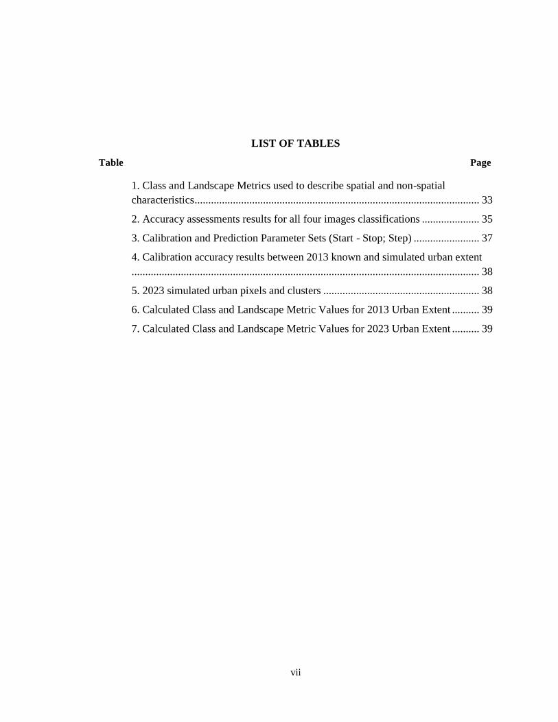
LIST OF TABLES
Table Page
1. Class and Landscape Metrics used to describe spatial and non-spatial
characteristics ........................................................................................................ 33
2. Accuracy assessments results for all four images classifications ..................... 35
3. Calibration and Prediction Parameter Sets (Start - Stop; Step) ........................ 37
4. Calibration accuracy results between 2013 known and simulated urban extent
............................................................................................................................... 38
5. 2023 simulated urban pixels and clusters ......................................................... 38
6. Calculated Class and Landscape Metric Values for 2013 Urban Extent .......... 39
7. Calculated Class and Landscape Metric Values for 2023 Urban Extent .......... 39
viii
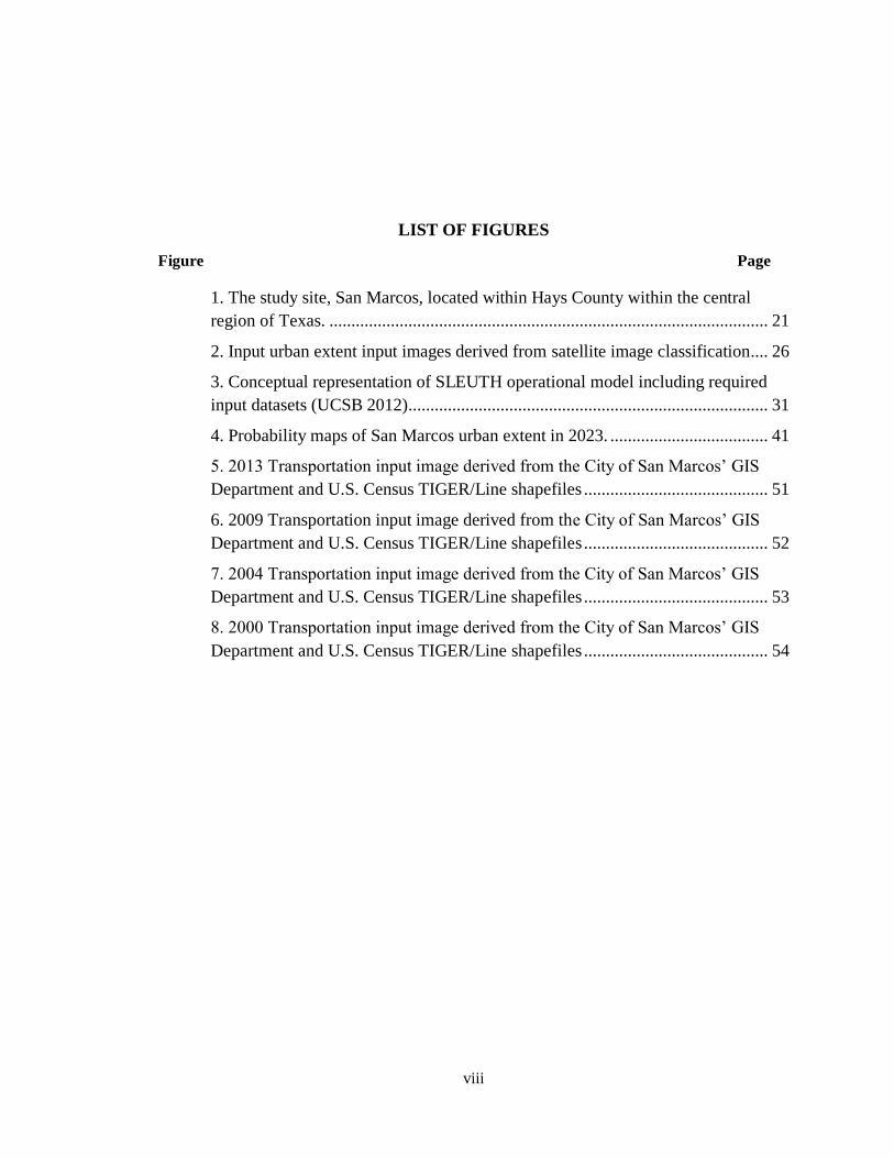
LIST OF FIGURES
Figure Page
1. The study site, San Marcos, located within Hays County within the central
region of Texas. .................................................................................................... 21
2. Input urban extent input images derived from satellite image classification .... 26
3. Conceptual representation of SLEUTH operational model including required
input datasets (UCSB 2012).................................................................................. 31
4. Probability maps of San Marcos urban extent in 2023. .................................... 41
5. 2013 Transportation input image derived from the City of San Marcos’ GIS
Department and U.S. Census TIGER/Line shapefiles .......................................... 51
6. 2009 Transportation input image derived from the City of San Marcos’ GIS
Department and U.S. Census TIGER/Line shapefiles .......................................... 52
7. 2004 Transportation input image derived from the City of San Marcos’ GIS
Department and U.S. Census TIGER/Line shapefiles .......................................... 53
8. 2000 Transportation input image derived from the City of San Marcos’ GIS
Department and U.S. Census TIGER/Line shapefiles .......................................... 54

1
1.0 INTRODUCTION
Within the past 20 years, Texas has become one of the fastest growing states in
the United States. The Capital Areas Council of Governments’ (CAPCOG) Assessment
of Growth and Development (2010) describes counties in the central Texas region as
having experienced unprecedented growth in recent years. Between 1990 and 2010,
population doubled from 919,000 to 1.8 million, and increased nearly 43 percent between
2000 and 2011. This strong regional population growth trend is expected to continue at
approximately 50,000 people per year, such that half of the region’s counties are
projected to have double-digit percent growth (CAPCOG 2010). At this rate, population
totals are estimated to increase to 4.1 million in 2040. Satellite cities of major
metropolitan areas have exhibited massive population growth as well. For example, Kyle,
Texas, 32 km south of Austin on the IH-35 corridor had a population increase of 427
percent from 5,300 in 2000 to 28,000 in 2010 (U.S. Bureau of the Census 2012).
Counties in the central Texas region do not have adequate land use administrative powers
to ensure future urban development is suitable for the region’s long-term needs.
Consequently, cities, which do have land use control, often plan land use development in
isolation (CAPCOG 2010). Despite this lack of coordination between city and county
planning agendas, the rapid urban growth in the region has piqued the interest of
governmental entities and non-governmental organizations.
Similar to many other large urban centers throughout the world, the in-migration
of residents from throughout Texas, the United States, and immigration from other
countries is responsible for the rapid growth of the Central Texas Region (CAPCOG
2010). Past trends in population growth in Texas suggest that more people are moving

2
from rural to urban areas. Between 2000 and 2005, 11 Texas counties with one or more
urban areas had at least 20 percent growth in population, while 93 rural counties
experienced losses in population (Texas Comptroller of Public Accounts 2008). Residents of
other states, such as California and New York, are drawn to Texas due to increased
employment opportunities and economic advantages such as lack of state income taxes
(Sager 2013). Additionally, many communities throughout the United States have
struggled from recent economic downturns; however, the unemployment rate for the
Central Texas region has remained two percent lower than the national average
(CAPCOG 2012).
Agencies such as CAPCOG and The Trust for Public Land (TPL) have released
assessments on the current growth trends of the area and expressing the need for
sustainable urban growth management. Beyond the urban problems associated with
population growth, there are additional environmental problems that should be
considered regarding the overall effects of urbanization. Generally, environmental
impacts of urbanization include habitat fragmentation (Scolozzi and Geneletti 2012;
Shrestha et al. 2012), biochemical and physical changes to the hydrological system
(White 2006), increased surface runoff and decreased aquifer recharge (Jacobson 2011;
Pappas et al. 2008), reduction of CO2 sequestration (Zhang et al. 2012), and urban heat
island effects (Radhi et al. 2013). Impervious surfaces such as buildings, roads, and other
paved surfaces prevent water infiltration into the soil and increase water runoff, thus
resulting in increased erosion and potential for downstream flooding (Jacobson 2011;
Pappas et al. 2008; White 2006). The non-contiguous conversion of native land cover
creates a fragmented landscape that reduces viable habitat for native fauna and flora

3
species (Scolozzi and Geneletti 2012; Shrestha et al. 2012). Additionally, the conversion
of vegetated land to urban cover exacerbates urban heat island effects and inhibits local
CO2 sequestration (Radhi et al. 2013; Zhang et al. 2012).
Unanimously, CAPCOG and TPL reports agree that the most pressing issues for
managing urban growth in the central Texas region include access to water, improvement
to transportation, land use management, and preservation of green spaces as some of
main factors to consider for promoting sustainable growth. Proper management and
consideration of these resources and infrastructure may provide a solid foundation for the
economic development necessary for continued population growth in this region.
The city of San Marcos, Texas is no exception to this unprecedented population
and urban growth. San Marcos is situated off the IH-35 corridor, just 48 km south of
Austin and 97 km north of San Antonio; two of the fastest growing metropolitan areas of
Texas. From 2000 to 2010, the total population of San Marcos increased nearly 30
percent from 34,700 to 44,900, respectively (U.S. Bureau of the Census 2012). A great
deal of this increase in population may be attributed to the growth in the student
population of Texas State University located within the city. Enrollment at Texas State
exhibited a steady increase throughout the past decade, with a notable increase of 4.7
percent in fall 2011 to 34,113 from 32,572 in fall 2010 (TXSU 2012b). This increase in
student enrollment is significant compared to the 2.2 percent increase in enrollment at
University of Texas at Austin for the same period (UT 2012).
1.1 Problem Statement
The urban coverage of San Marcos is expected to expand to permit the needs of a
growing population and will warrant a greater expenditure of local resources. With the

4
projected growth of population and urban coverage alike, local governmental and non-
governmental organizations could benefit from information pertaining to the projected
amount and location of urban growth. Models, such as the Cellular automata based
SLEUTH model, are one such tool that can forecast urban growth patterns that can be
utilized by decision-makers for urban planning considerations.
1.2 Objectives
This study will address two main objectives:
1. Describe regional changes in urban cover within the study area beginning in
2000 and ending in 2013, and
2. Implement the SLEUTH urban growth model to produce a probability map of
urban coverage for San Marcos, TX in the year 2023.
1.3 Justification
Both Texas State and the city of San Marcos facilitate rapid population growth
through policy and urban development. The city of San Marcos is encouraging economic
development by offering new business incentives, development fee waivers, and tax
waivers (City of San Marcos 2012). These incentives exist to attract new businesses
investments, which in turn may result in property development and increased
employment opportunities. Similarly, Texas State has invested over $585 million in
improvements and new developments to the university campus (TXSU 2012a). These
campus developments are designed to bring greater academic attention to the university,
increase student enrollment, and, therefore, the overall population of San Marcos.
Beyond the measurement of urban growth, the full impact of urban expansion can be
5
realized by considering the need for water, building materials, food, and other goods
pulled from the surrounding region to facilitate population and urban growth. As a result,
the surrounding region is often converted from natural land to agricultural land (where
permissible), and, through time, agricultural land is converted to urban cover.
Monitoring the expansion of urban areas is of critical importance to those
involved in the study and management of the processes that influence such growth.
Simply put, the greater the population within a region, the greater the impact on the
environment through the consumption of food, energy, water, and land (Soltész 2010). As
urban areas continue to expand to facilitate the population growth and resource needs,
many areas previously used for agricultural or other green spaces are converted to urban
cover (Bagan and Yamagata 2012; Li et al. 2010; Sezgin and Varol 2012; Yang 2002).
Thus, accurate assessments of urban growth are important to understand the
environmental impacts over time and to guide sustainable growth such that negative
impacts on the environment are mitigated (Han et al. 2008).
6
2.0 LITERATURE REVIEW
2.1 Overview
Factors that influence growth of urban areas are complex with varying degrees of
interdependence. Thus, simulating this complex process and accounting for key factors
fostering such growth is challenging (Barredo et al., 2003). Models are a way of
representing a process in reality composed of many complex relationships into a
simplified version that is composed of the most significant factors perceived to influence
a particular process (Liu 2009). Researchers construct models to represent the structure or
process of a real system in an effort to understand, explain, or predict the behavior of the
system (Liu 2009). A key feature and benefit of modeling is the ability to construct the
model using key elements believed to influence a process. This selectiveness eliminates
noise of other, less important factors and enables the real world to be simplified in a valid
and understandable way. A challenge to constructing a model, however, involves the
decision of the selecting elements of a real-world system to are perceived to be important
and must be included and adequately interrelated to create valid results (Liu 2009).
The establishment of known relationships among elements included in a model
enables researchers to make predictions of future conditions. As data used in models are
generated from empirical observations, modeling results should be applicable to the real
world. It should be noted here, however, that models are only approximations of reality
and that any subsequent predictions can only be interpreted as generalizations of future
conditions (Liu 2009). As many Earth processes are highly dynamic and complex, the use
of geospatial models have been widely applied to help researchers gain more insight in to
the causes of such phenomena. Common examples of geospatial modeling include
7
hydrological (Remo et al., 2009), ecological (Silva et al., 2008; Zhao et al., 2006), land
cover change (Araya and Cabral, 2010; Bagan and Yamagata, 2012; Yang, 2002) and
urban development (Cheng and Masser 2003; Jantz et al., 2010, Liu, 2009; Yang, 2002).
The adequacy of these models is highly dependent on the quality and accuracy of the data
used. Currently, there is a great deal of research in determining the optimal methods of
analysis to generate the most accurate output results.
Urban growth modeling is a common method used to help researchers attempt to
understand the underlying factors influencing urban growth. Understanding the
complexity of urban growth and expansion is a heavily researched topic (Barredo et al.
2003; Cheng and Masser 2003; Clarke et al. 1997; Cohen 2006; Geohegan 2001; Liu
2009; Santé et al. 2010; Soltész 2010). A review of this relevant literature reveals a set of
characteristics describing urban expansion that are common among all cases. Developing
urban systems can be characterized as self-organizing, complex emergent systems in
which the collective interactions at the local-scale will shape and determine the ordered
patterns at the large-scale (Tobler 1979; Wolfram 1984). Self-organization is defined as a
process that typically involves emergent properties where coherent and organized
patterns arise over time from the local interactions of an initially disordered system. The
degree of interdependence of the processes within a system is not completely known;
however, it is through these relationships that systems will tend to develop patterns
(Barredo et al., 2003).
Geographic information systems (GIS) and remote sensing technologies are the
most commonly utilized tools in geospatial modeling. GIS serves as a platform for
quantitative and qualitative analysis of geospatial data. The application of GIS
8
technologies is well known to be a means of efficiently analyzing large amounts of
spatial data. However, in order to make predictions of future conditions, one must first
have a good understanding of the historical patterns of change leading up to present
conditions. Remotely sensed data are well suited for land cover land use (LCLU) change
detection because of its repetitive acquisition capabilities and ability to cover a large
spatial extent. Therefore, remotely sensed images are often used as the basis for LCLU
maps analyzed within a GIS.
2.2 Remote Sensing for LCLU Change Detection
The U.S. Geological Survey (USGS) has long been on the forefront of studying
land-use and land-cover changes. Since the 1970s with the development of a land-cover
and land-use classification system by Anderson et al. (1976), the USGS has maintained
an interest in monitoring the changes over the Earth’s surface. In the 1990s, the USGS
began the Human-Induced Land Transformations (HILT) project that was initially aimed
at understanding the transitions of land to urban land-use, specifically in the San
Francisco/ Sacramento area (Acevedo et al. 2010; Clarke et al. 1997; Kirtland et al.
2010). The results of the HILT project showed that the integration of historical maps and
related geographic information with remotely sensed data can successfully map urban
land characteristics, as well as provide a visual representation of such changes through
time (Acevedo et al. 2010).
A good change detection study, as determined by Lu et al. (2004), should provide
the following information: area change and change rate, spatial distribution of changed
types, change trajectories of land-cover types, and accuracy assessment of change
detection. Traditional methods of change detection began with repeat photography and,

9
through timely technological advances, have eventually evolved to using digital remote
sensing data. As technology continues to progress, the scientific community continues to
develop new methods with increasingly accurate information on the changes to the
Earth’s surface.
There are many characteristics of remotely sensed data that make them
particularly well suited for change detection projects. Currently, there are dozens of
existing remote sensing platforms, all of which collect a variety of multispectral
information at varying spatial scales (Jensen 2005). Satellite remote sensing platforms,
such as Landsat Thematic Mapper (TM), Landsat Multi-Spectral Scanner (MSS), Landsat
Enhanced Thematic Mapper Plus (ETM+), Satellite Pour l’Observationde la Terre
(SPOT), Advanced Very High Resolution Radiometer (AVHRR), Moderate Resolution
Imaging Spectroradiometer (MODIS), and Advanced Spaceborne Thermal Emission and
Reflectance Radiometer (ASTER) are all major sources of data for change detection
applications (Jensen 2005; Lu et al. 2004). These platforms are consistent and reliable
sources of data with known temporal and spatial resolutions (Jensen 2005). Additionally,
airborne (sub-orbital) remote sensing platforms, such as Compact Airborne
Spectrographic Imager (CASI), are capable of capturing data at intervals that a particular
satellite cannot (Jensen 2005).
The synoptic view of satellite and airborne sensors also allows for data to be
collected over large areas, making it possible to detect changes over a large region. For
example, Zhou et al. (2011) acquired five images from Landsat TM, MSS, ETM+, and
SPOT HRV (high resolution visible image) to determine land-use changes and the human
impacts on the land over 30 years in a region of China. Their results show that until the
10
early 1990s human impacts were minimal, however, since then the area of cultivated
farmland increased over five times, and continues to do so 30 percent annually. This
research highlights the use of multitemporal remote sensing data sets for detecting
changes across a large area over a relatively long period.
It is important to consider the sensor selected to obtain data for specific
applications, as all sensors provide specific spectral and spatial data with varying
resolutions (Jensen 2005). The digital format of remote sensing data makes it easy to
store and is suitable for computer processing (Lu et al. 2004). After selecting the image
data, the next step, selecting the appropriate change detection method, is perhaps the most
important consideration for generating accurate results (Lu et al. 2004; Lu et al. 2005).
Lu et al. (2005) analyzed the differences in land-cover change detection
accuracies generated from ten binary change detection methods using Landsat 5 TM
imagery over a study site in the Amazon tropical region. Their results indicate that three
of the ten techniques produce significantly better results. Furthermore, these results
exemplify the importance of selecting the appropriate change detection technique to
produce the best results for a specific study area.
Lu et al. (2004) and Singh (1989) provide in-depth reviews of the many available
change detection techniques available at their respective times of publishing. These
studies show the abundant methods available for comparing data between images for a
diverse set of applications. Lu et al. (2004) identified the major categories of change
detection applications using remote sensing technology, including LULC change, forest
or vegetation change, wetland change, forest fire, urban change, environmental change,

11
and many other applications. These reviews underscore the importance of monitoring the
changes on the Earth throughout the years and the broad applicability of remote sensing
data for change detection studies. It is not surprising that significant effort has gone into
the development of new technology and methods for various change detection
applications.
Change detection projects provide timely and accurate information on the changes
of Earth’s surface features and allow us to have a better understanding of the
relationships among humans and our environment (Lu et al. 2004). Remote sensing
technology has been utilized for many change detection studies throughout the years,
fostering the advancement of change detection techniques for various applications.
Despite this, characterizing the volumetric changes of target features using traditional
photogrammetric methods is labor intensive and time consuming (Lefsky et al. 2002).
Nonetheless, results of change detection studies are broadly applicable to anyone who is
interested in any visible changes on the earth over time. Examples of applications include
land-use and land-cover change, forest or vegetation change, forest fire, wetland change,
urban change, environmental change, and many others.
2.3 Overview of Urban Growth Modeling
Most early applications of understanding the urban processes used transportation
and land-use information to create models that were based on gravity theory or some
form of optimized mathematics (Santé et al. 2010). However, among all urban modeling
techniques, cellular automata (CA) are particularly well suited for modeling complex and
dynamic natural phenomena such as urban areas (Tobler 1979; Wolfram 1984). Tobler
(1979) identified the potential application of cellular space models to geographical

12
processes. Tobler (1979) proposed that changes in the patterns on the Earth’s surface are
analogous to a game of chess in which the rules are simple, yet using these rules as
strategy makes the game complex. In this context, given an initial state, a desired state,
and a set of transition rules, one must determine if there is an identifiable path from one
state to another (Tobler 1979). Wolfram (1984) demonstrated that CA are capable of
modeling complex systems and are most appropriate in highly nonlinear processes, such
as biological and physical systems, where growth inhibition effects occur.
More recent conceptual and technological advances have led to increased CA
research and development of models applicable to real-world urban systems. CA models
have the ability to simulate urban growth through the assumption that past urban
development affects future urban growth patterns through neighboring interactions
between land-uses (Santé et al. 2010).
Liu (2009) defines and explains the five basic elements of cellular automation: the
cell, the state, the neighborhood, the transition rule, and the time. Cellular automata
operate on a raster-format of discrete cells, each characterized by a state, where the state
is representative of any one specific land cover or land use, such as rural or urban. This
format allows for easy integration with GIS, and, consequently, operates at high
computational efficiency at relatively fine spatial resolutions. The state of each cell is
dependent on its previous state, the state of neighboring cells, and set of transition rules
(Barredo et al. 2003; Garcia et al. 2012; Santé et al. 2010). The complexity of urban
simulation requires considering particular behaviors of urban systems and modifying (or
relaxing) the original structure of the CA to compensate for such complexity.

13
A major benefit of cellular automata is its ability to model complicated behavior,
given its relatively simple construction (Wolfram 1984). A cellular automata system
operates by dividing space into a regular cell spatial tessellation, where each cell is
assigned a specific state. The status of each cell is determined by the state of the cell itself
and the state of the other cells within a local neighborhood. Statuses of each cell change
synchronously based on a defined set of local transition rules. All cells together, with the
combined effect of single cell transition rules, define and generate the whole complex
system where changes occur with each discrete time step (Liu 2009; Silva et al. 2008).
Another beneficial component of cellular automata is its ability to model the
characteristics of a system that is capable of self-organization. Self-organization is a
characteristic found in many complex systems, such as cities, in which local-scale
interactions continue existing patterns, but also generate new patterns that participate in
the next iteration; much like a feedback mechanism (Barredo et al. 2003). Cellular
automata are able to accommodate this self-organization characteristic by allowing rules
to change as the system grows (Clarke et al. 1997).
The concept of cellular automata can be easily applied to the organization and
development patterns of urban areas. Consider that an urban area is represented by
cellular space in which each cell is representative of a specific land parcel within the
urban area. Each cell state can be defined as urban or non-urban at a specific point in
time. The probability land development, or a cell's status changing from non-urban to
urban, is influenced by the collective status of a local neighborhood of cells and a set of
defined transition rules. These transition rules, usually expressed as "If-Then" statements,
14
determine the process of a land parcel, or cell, transitioning from one state to another (Liu
2009).
For example, if three or more urban cells surround a non-urban cell, then the non-
urban cell will likely convert to an urban cell through a growth cycle. This is, however,
just a simple example of one transition rule. In the real-world most geographic
phenomena, such as urban development, do not follow a uniform development process
and requires developing multiple locally defined transition rules that take in to account
multiple geographical conditions. Urban areas are composed of a complex mix of related
units, but the degree and nature of the connections can be difficult to determine. The
dynamics of urban land use in an urban area is directly attributable to the decisions of
individuals, public, and private corporations acting together over time (Barredo et al.
2003). As a result, cities are continuously organized and shaped based on these
influences. Barredo et al. (2003) identified five groups of factors that can influence the
allocations and decision-making process of urban land-uses: environmental
characteristics; local-scale neighborhoods characteristics; spatial characteristics of the
cities (i.e. accessibility); urban and regional planning policies; factors related to
individual preferences, level of economic development, socio-economic and political
systems.
Santé et al. (2010) provides an in-depth review of many of the common
modifications of CA for urban simulations and provides examples of the main urban CA
models applied to real-world urban development processes. Additionally, CA-based
models for urban growth simulation are grouped and compared based on the main
characteristics of the model. Garcia et al. (2010) assesses the operational practicability of
15
three common urban CA models to simulate the growth of a town in Spain. Their results
showed that low growth in the area over the study period warrants more information with
greater detailed data in order to identify growth dynamics within the area. However,
including additional land-uses and extending the neighborhood of cell interactions could
improve simulation results. This research provides context into the strengths and
weaknesses of various models and underscores the application of a diversity of CA-based
models for understanding various complex urban systems.
2.4 Incorporation of Remote Sensing LCLU Change Detection and Urban Growth
Modeling
The systematic analysis of the dynamic changes between non-urban land cover to
urban, or other land covers associated with urban expansion, can reveal trends that begin
to explain past development patterns, as well as improve predictions of future growth.
Remotely sensed imagery has been widely applied for the systematic analysis of changes
in land cover and land use relative to changing urban growth characteristics. Bagan and
Yamagata (2012) integrated Landsat MSS, TM, and ETM + derived land cover maps
with population density to determine relationships between the land-cover and population
density changes based on grid cells each covering 1 km2. Population statistics were
generated per grid cell by linking census data to the appropriate cell using latitude and
longitude coordinates. Results demonstrated a decrease in growth within the metropolitan
core area, a strong positive relationship between urban expansion and population density,
and a strong negative relationship between urban expansion and cropland change.
Additionally, urban growth exceeded population growth by a factor of approximately 2.6.

16
Hepinstall-Cymerman et al. (2009) developed a set of multi-date land cover maps
for an urban area using Landsat TM images to examine the change in composition and
configuration of land covers over a twenty-year time span. Images were classified using a
combination of image classification techniques including image segmentation, spectral
unmixing, and supervised classification. Image classification results were refined using
multi-season imagery using landscape trajectory rules and ancillary GIS data. Changes in
land covers through the study periods are described using landscape metrics of
composition and configuration. Results from this study are similar to other findings;
urban patches grow in size and become less dispersed with a subsequent decrease in the
extent and homogeneity of grass, agriculture, and forest land cover.
An understanding of historic land cover change is a prerequisite to predictions of
future urban land cover characteristics. Other studies have applied LULC maps derived
from remotely sensed imagery to model and predict future conditions of class coverage.
Tewolde and Cabral (2011) used eCognition to perform an object-based classification of
Landsat 5 TM imagery into six basic land cover classes. Changes in urban sprawl were
analyzed and quantified using post-classification change detection, land change modeler
(LCM), and Shannon’s Entropy, an urban sprawl index. Land cover maps were analyzed
through the LCM to determine the main variables responsible for growth. The multilayer
perceptron (MLP) neural network algorithm is used to create maps of cell transition
potential that are subsequently used with Markov Chain modeler to simulate future land
cover extents. The model simulation is validated by a comparative analysis of the
predicted map to the reference map based on Kappa variations. Following the trends of
17
similar studies, the study area has experienced, and is simulated to continue to experience
rapid urban growth at the expense of valuable periphery resource lands.
Araya and Cabral (2010) conducted a comparable study with similar results. In
this study, spatial metrics and Shannon’s entropy were used to describe the spatial
characteristics of class patches, class area, and the landscape. Modeling changes in
classes was evaluated using a combination of Markov Chain and CA. The Markov Chain
analysis is useful for describing the probability of land cover changes from one period to
the next. The CA component allows for the integration of the transitional probabilities.
This research highlights the utility of CA models to consider the dynamic transitional
characteristics that will vary from one region to another.
Although there are several LULC modeling tools available, each with their own
advantages and disadvantages, the SLEUTH model is capable of simulating changes in
urban form independently, or in concert with LCLU data or socioeconomic variables.
Development of the SLEUTH model comes from the modification of a wildfire model
developed by Clarke et al. (1994) that established principles and growth rules to simulate
organic growth based on CA research by Batty and Xie (1994), Couclelis (1985), and
others. Based on these principles and rules, Clarke et al. (1996) developed SLEUTH, a
CA-based urban growth simulation model as part of the USGS HILT project to estimate
the regional impacts of urbanization. The SLEUTH model includes neighborhood
transition rules that are typical of CA models, but operates with multiple data sources that
are believed to be major influences on the process of urban growth including topography
(slope and hillshade), road networks, existing settlements, excluded zones, and LCLU.
These data sources are included as layers in the modeling process and all (except for

18
hillshade) influence the way urban and other LCLUs change over time (Mahiny and
Clarke 2012).
Clarke et al. (1996; 1997) and Clarke and Gaydos (1998) define and discuss five
factors that control the behavior of the system and the four type of growth that all
together create an urban growth simulation that is unique to an individual region of
interest. The five factors controlling system behavior include: “a diffusion factor which
determines the overall dispersiveness of the distribution both of single grid cells and in
the movement of new settlements outward through the road system; a breed coefficient
which determines how likely a newly generated detached settlement is to begin is town
growth cycle; a spread coefficient which controls how much normal outward ‘organic’
expansion takes place within the system; a slope resistance factor which influences the
likelihood of settlement extending up steeper slopes; and road gravity factor which has
the effect of attracting new settlements onto the existing road system if the fall within a
given distance of the road” (Clarke et al. 1997, 252). The growth rate of an urban area is
the result of the combination of four different types of urban growth: spontaneous,
diffusive, organic, and road influenced (Clarke et al. 1996, Clarke et al. 1997, Clarke and
Gaydos 1998).
SLEUTH allows for predictive modeling under different scenarios matching
urban planning objective, or lack thereof (Feng et al. 2012, Jantz et al. 2010). Jantz et al.
(2010) developed a new version of the SLEUTH model (SLEUTH-3r) including a
method to expand the utility of the SLEUTH model to include economic, cultural, and
policy variables, as well as other modifications including new calibration statistics,
decreased memory requirements, and enhanced scale sensitivity. Their study area

19
covered encompassed 257,000 km2 divided into 15 sub-regions of 7100 km
2 to 23,000
km2, each with a unique set of calibration values. Urban growth, simulated for a twenty-
year period, was forecasted under current growth trends for each sub-region and other
model scenarios created to simulate urban growth under different economic, cultural, and
policy regimens by relative changes in calibration values. Calibration results of the
SLEUTH-3r model show a match within 10 percent of the simulated map to the control
map. The Jantz et al. (2010) study demonstrates the capability of the SLEUTH-3r model
to adapt to a range of local conditions, while at the same time facilitating the discovery of
the impacts of the human socio-economic decision-making on urban development. Other
studies cited by Mahiny and Clarke (2012) describe the ease of linking environmental
data to model predictions by making appropriate changes to input layers to reflect study
area conditions or urban planning objectives.
Measurement of urban area shape, size and configuration is important to for land-
use planning and development. A systematic measurement of built-up area can aid in
establishing relationships between growth and the process of such growth (Yeh and Li
2001). Furthermore, knowing the probability of land conversion of resource land
(agriculture, forest) to residential, commercial, or industrial uses will guide development
planning to seek alternative or preventative measure to protect resources (Araya and
Cabral 2010, Hepinstall-Cymerman et al. 2009; Jantz et al. 2010, Tewolde and Cabral
2011). The spatio-temporal processes of urban development and the resulting social and
environmental consequences of this development deserve a great deal of attention from
urban geographers and policy makers (Liu 2009).

20
3.0 MATERIALS AND METHODS
3.1 Study Area
San Marcos, the county seat of Hays County, Texas (Figure 1) is located in the
southeastern corner of the county along the IH-35 corridor between Austin and San
Antonio, two of the fastest growing cities in the U.S. The city limits encompass
approximately 4,700 ha and contains land east and west of IH-35. The main campus of
Texas State, located within the city, covers 185 ha, nearly four percent of the land area
within city limits. The city is positioned on the Balcones Escarpment separating the
Edwards Plateau to the west and the Blackland Prairies to the east. This unique location
at the foot of the Edwards Escarpment provides the headwaters for the spring fed Spring
Lake and San Marcos River that transect the city. In fact, Native American artifacts found
around Spring Lake are evidence that this area is one of the oldest and longest inhabited
locations in the United States (Hickey 2011).

21
Figure 1. The study site, San Marcos, located within Hays County within the central
region of Texas.

22
Within the context of urban growth, there are unique characteristics of San Marcos
that make the city a good candidate for this study:
San Marcos’ close proximity to IH-35 is a source of continuous human and
economic resources to the city. Beyond the historical trends of urban growth
following main transportation lines, the location of the city between Austin and
San Antonio intensifies capital resources.
Since incorporation of San Marcos in 1877 and the opening of the Southwest
Texas State Normal School in 1903, growth of the city and school are related. The
influence of the university on economic and urban development within the city is
a contributing factor not common in most developing cities.
The local topography is not uniform across the entire study area. A dynamic range
in slope will influence and produce unique growth patterns where new
development must follow the path of least topographic resistance.
San Marcos currently contains approximately 550 ha of parkland and local natural
spaces, much of it sharing borders with the San Marcos River or its tributaries.
These natural areas have and will continue to be a source of revenue for the city
and can limit growth in certain areas that some would consider attractive for
development.
These unique characteristics of San Marcos fit well with the data requirements of the
SLEUTH model and will require case-specific consideration during model calibration.

23
3.2 Geospatial Data and Pre-processing
The SLEUTH model operates from six input grayscale gif images: urban extent,
transportation, excluded areas from urbanization, slope, and hillshade are all required.
The sixth layer, land use, is optional and is not used in this study. Additionally, there are
format standards for all dataset images. For this study, all input images are projected to
Texas State Plane Coordinate System using the Lambert Conformal Conic zone 4204
(meters) with the North American Datum of 1983. All images have a 30 m spatial
resolution and are composed of 990 columns and 906 rows of pixels. Four discrete time
periods of data are required for statistical calibration of the model.
3.2.1 Urban
Landsat 8 and Landsat 5 TM digital images at 30 m spatial resolution were
collected for the study area for four time periods across the scope of the study; 2000,
2004, 2009, and 2013. Landsat 8 imagery was used for 2013 due to the decommissioning
of Landsat 5 TM in 2011 and the Scan Line Corrector failure of Landsat 7 ETM+ in
2003. All images were collected from EarthExplorer, a USGS web-based repository for
all Landsat and other sensor’s imagery. An object-oriented supervised classification was
performed in eCognition Definiens 8 to produce urban land cover datasets for each
calibration year. eCognition is an object-oriented image analysis software that extracts
features based on spectral and/or textural attributes. Object-based classification is
advantageous compared to pixel-based classification as it allows the user to analyze
imagery based on image objects rather than on a pixel level (Araya and Cabral 2010,
Tewolde and Cabral 2011). eCognition operates by segmenting groups of image pixels
that share similar properties based on a set of threshold values, or rules defined by the
24
user. Additionally, classification results can be exported as raster or vector formats that
are easily integrated into a GIS.
Supervised classification implemented the nearest neighbor classification
algorithm. Extracted segments were classified based on user-specific samples and a set of
spectral and textural conditions. These conditions are adjusted to best suit a specific land
cover and are saved for use on subsequent images of the same area. Image segments were
classified as urban and non-urban. The Multi-resolution Land Characteristics Consortium
(MRLC) Level 1 classification scheme is used to distinguish different levels of urban
cover intensity (Anderson et al. 1972). Low-density urban areas were not included in the
urban extent layer. Low-density urban areas are found primarily outside of the city limits
and consist of lots or developments with considerable acreage separating each house or
areas with small groupings of multiple houses. These areas were difficult to distinguish
from the surrounding areas during image segmentation due to their proportional coverage
to the surrounding vegetation. Medium and high-density urban areas are both included in
the urban cover layer. The study area was extended to a best-fit square around the San
Marcos extraterritorial jurisdiction to allow for the forecasting of extended urban growth
outside of San Marcos city limits and for consistency in the number of pixel columns and
rows of each input image. Consequently, smaller municipalities that now fall within the
study area, including Martindale, Staples, Uhland, Reedville, Redwood, Hunter, and
Maxwell were also included in the urban cover layer.
Accuracy assessments of urban and non-urban land cover classifications were
performed for classified image. Accuracy assessment is necessary due to the multiple
applications of results for model simulation assessment and other data requirements for

25
the model. Kappa statistics and confusion matrices were used to assess overall accuracies
and to validate classification results. Only classified images with Kappa values greater
than or equal to 0.8 were considered acceptable for use in further analysis. A Kappa score
of 0.8 (80 percent) or higher is considered indicative of a strong agreement between the
classified image and reference samples. A high Kappa score provides the user/producer
assurance that land cover classifications are significantly better than if land cover
classifications were made by chance (Jensen 2005). A stratified random sample of 24
samples per land cover was used to populate the confusion matrix. This sample size was
calculated through a multinomial distribution with a 95 percent confidence level and ten
percent precision (Jensen 2005).
The same Landsat 8 and Landsat 5 TM images were used for both the collection
of samples for land cover classifications and for accuracy assessments. In-situ and high-
resolution imagery were not used for gathering classification samples as the difference
between high and medium-intensity urban and non-urban land covers are easily
distinguishable from visual image interpretation. Moreover, accuracy assessments of
image classifications warranted the use of the same imagery for the purpose of
segmentation identification. The image segmentation is unique to the individual image
and, therefore, requires reference to the originally segmented image during accuracy
assessments for identification of the correct land cover class.
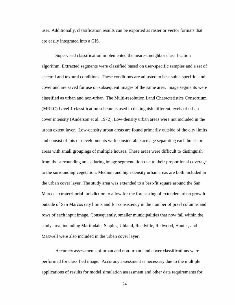
Each urban layer (Figure 2) was derived through the extraction of urban pixels
from land cover classification of images for each period. The urban image used as the
start date for the model, referred to at the seed layer, represents the initial conditions in
which further expansion will occur in subsequent iterations. All classified urban/non-
26
urban images were converted to grayscale GIF images using ArcGIS to make data
compatible for model operation.
Figure 2. Input urban extent input images derived from satellite image classification.
White represents urban, black represents non-urban pixels.
27
3.2.2 Excluded Area
The excluded area layer includes cells that represent areas protected from future
urbanization. The excluded layer is composed of rivers, streams, water bodies, parks,
railroads, and cultural areas. All data composing the excluded layer were obtained in
vector format, merged together, and then converted to raster format. Parks, cultural areas,
and railroads data were collected from CAPCOG. Hydrological datasets were gathered
from the USGS National Hydrography Dataset. A 30 m buffer surrounding the rivers and
streams was added to exclude these areas from any new urban development. These areas
fall within the water quality zone of 30 m, per City of San Marcos’ code of ordinances for
new development and is prohibited or very limited to development. All water bodies
smaller than 0.005 km2 were removed from the excluded areas as any water body larger
than that was believed to be beyond the cost benefit of infilling for new development.
Nearly all water bodies removed as a result of this operation were small cattle ponds on
the eastern side of the study area.
3.2.3 Transportation (Roads)
Roads are represented by an array of cells corresponding to roads present at each
specific period and with pixel values relative to accessibility. For example, pixels with
higher values represent roads with a tendency to attract urban growth. Road pixel values,
or weighting, are determined by using the functional classification system developed by
the U.S Department of Transportation Federal Highway Administration (2013). Roads
are grouped into classes according to the level of service and accessibility they are
intended to provide. This system provides an objective guideline for associating weights
with each road. Each road was categorized into one of three classes: arterial, collector, or
28
local roads. Arterial roads, given a pixel weight of 100, are the least common of the three
road classes and are designed to provide the fastest route of travel. Collector roads, the
second most common with a pixel weight of 50, are used as connections between arterial
and local roads and are equally accessible and mobile. Local roads, with a pixel weight of
25, have high accessibility, but low mobility and are the most common class of roads.
Transportation networks can have a major influence on regional development.
Thus, several road layers are desired to represent a change with the city’s growth through
time. These road layers (shown in Appendix A) were read into the model as time
progressed to represent the most up-to-date transportation system for a particular period.
Historic and current road data were collected as shapefiles from the City of San Marcos’
GIS Department and U.S. Census TIGER/Line shapefiles. The vector road data were
converted to GIF images with pixel values adjusted to represent road influence and
accessibility.
3.2.4 Slope
The slope layer is used for establishing a slope-resistance weighting that
determines the maximum change in elevation where urban expansion or new settlement
can take place. To match the requirements of the SLEUTH model, slope values represent
percent slope and were calculated from a 2009 USGS 7.5-minute digital elevation model
(DEM).
29
3.2.5 Hillshade
The hillshade layer is a static background image included with image outputs of
forecasted urban extent to provide a spatial perspective to changes in urban extent over
time. Similar to slope, the hillshade image was generated using the 2009 USGS 7.5-
minute DEM.
3.3 SLEUTH Model Calibration
A major component to SLEUTH implementation and accurate reproduction of
past land cover changes is through calibration of parameter values to match local
conditions of the study area. Thus, determining the best fit of appropriate parameter
values is highly important with regard to simulating future conditions. Five coefficient
values affect the simulated growth of a study area: diffusion, breed, spread, slope, and
road gravity. The model was calibrated using the “brute force” Monte Carlo methodology
in which a large number of coefficient values are generated and tested, resulting in an
output of fit statistics for the user to evaluate. Output statistics include several Pearson r2
statistics that compare measurements between known historical data and simulated data
such as number of urban pixels, edges, clusters, and spatial match comparison. One such
output statistic is a shape index named the Lee Sallee metric, which is a measure of
spatial fit between the simulated urban growth and known urban growth (KantaKumar et
al. 2011). While the Lee Salle metric has been used in previous studies for SLEUTH
model calibration, studies have shown the Lee Sallee metric to have a relatively poor
association with urban growth (Dietzel and Clarke 2007, KantaKumar et al. 2011). The
Optimum SLEUTH Metric (OSM), a metric developed by Dietzel and Clarke (2007),
produces a value based on compare, population, edges, clusters, slope, Xmean, and
30
Ymean metrics and “will provide the most robust results for SLEUTH calibration”
(Dietzel and Clarke 2007, 43). OSM values are the product of multiple correlation
coefficients, thus the resulting OSM values share the same minimum and maximum
values ranging between zero and one. The highest OSM values can be used to narrow
down the range of calibration values that creates the best fit between known and
simulated urban growth.
Calibration begins with a set of starting coefficient values that are slightly
modified by a process of self-modification through each calibration cycle. Calibration of
coefficient values for this study were produced through a series of calibration phases,
starting with coarse calibration. For coarse calibration, values for each parameter range
from 1-100, and are incremented in steps of 25. Jantz et al. (2010) noted that any
additional testing of parameter values than those tested through the coarse calibration
warranted no additional gain at the cost of additional computing time. Coefficient values
are changed to simulate accelerated or depressed growth relative to local urban
development conditions for that point in time and result in a new set of coefficient values
at the end. The resulting values of the coarse calibration are further narrowed down
through fine and final calibration, where each set of refined coefficients are selected
using the range of best-fit values determined by the top five OSM values of the
antecedent calibration.
The final step of the calibration process is to determine the coefficient values that
most accurately simulate historic growth trends. The top OSM values calculated after the
final calibration are used to initialize the model for forecasting land cover conditions.
Additionally, coefficient values used in predictions of urban extent for 2023 were run
31
with 1,000 Monte Carlo iterations to account for any inherent variability in the modeling
results.
3.4 Urban Growth Change Modeling
The SLEUTH model was applied to forecast and characterize the growth of urban
land cover for a twenty three-year period. Growth was characterized by evaluating the
conversion of non-urban to urban cover through time using urban growth maps,
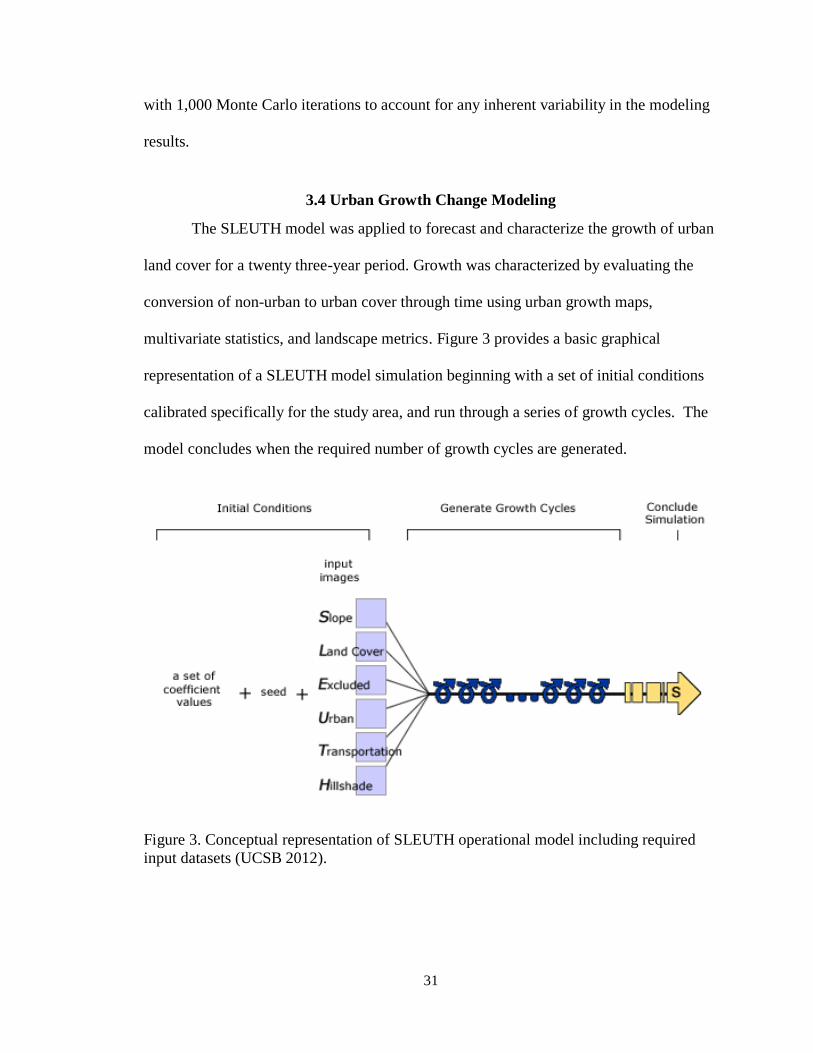
multivariate statistics, and landscape metrics. Figure 3 provides a basic graphical
representation of a SLEUTH model simulation beginning with a set of initial conditions
calibrated specifically for the study area, and run through a series of growth cycles. The
model concludes when the required number of growth cycles are generated.
Figure 3. Conceptual representation of SLEUTH operational model including required
input datasets (UCSB 2012).
32
3.4.1 Interpretation and Analysis of Results
Implementation of the SLEUTH model produces image and statistical output
files, each with varying details about the growth resulting from each growth cycle. Land
cover classification results were used as the control to test the calibration accuracy of
simulated urban growth. The number and percentage of urban pixels, and the number of
urban clusters were calculated for both the 2013 land cover classification and the 2023
simulated urban extent. The SLEUTH model conveniently outputs measurements of the
number of urban pixels and clusters for each simulated growth cycle. A fractional
difference metric was used to assess the difference between simulated and actual urban
areas where negative values indicate underestimation, positive values for overestimation,
and zero values for a perfect match.
Surface metrics are used to describe the spatial and non-spatial characteristics of
an area of interest through quantification of existing relationships between features on the
landscape. For example, the variability in the size of urban land-cover patches (non-
spatial) and the arrangement and location of these patches throughout the landscape
(spatial) (McGarigal et al. 2012). For this study, metrics were computed per land cover
class describing the pattern and distribution per class, and by landscape, where the spatial
structure of the entire surface may be described by a single metric. These metrics can be
easily computed on categorical (i.e., land cover) grids in FRAGSTATS (McGarigal et al.
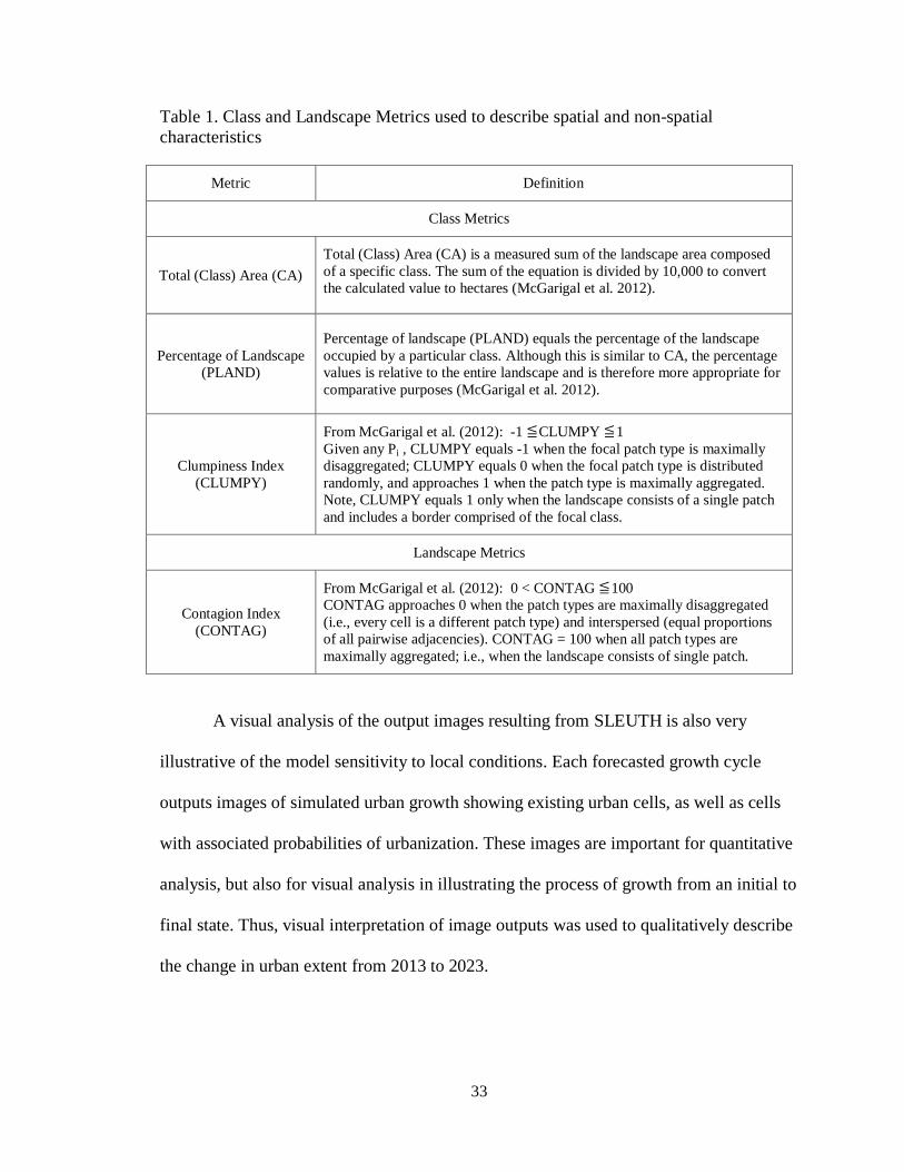
2012). Class and landscape metrics used in this study are provided in Table 1.
33
Table 1. Class and Landscape Metrics used to describe spatial and non-spatial
characteristics
Metric Definition
Class Metrics
Total (Class) Area (CA)
Total (Class) Area (CA) is a measured sum of the landscape area composed
of a specific class. The sum of the equation is divided by 10,000 to convert
the calculated value to hectares (McGarigal et al. 2012).
Percentage of Landscape
(PLAND)
Percentage of landscape (PLAND) equals the percentage of the landscape
occupied by a particular class. Although this is similar to CA, the percentage
values is relative to the entire landscape and is therefore more appropriate for
comparative purposes (McGarigal et al. 2012).
Clumpiness Index
(CLUMPY)
From McGarigal et al. (2012): -1 ≦ CLUMPY ≦ 1
Given any Pi , CLUMPY equals -1 when the focal patch type is maximally
disaggregated; CLUMPY equals 0 when the focal patch type is distributed
randomly, and approaches 1 when the patch type is maximally aggregated.
Note, CLUMPY equals 1 only when the landscape consists of a single patch
and includes a border comprised of the focal class.
Landscape Metrics
Contagion Index
(CONTAG)
From McGarigal et al. (2012): 0 < CONTAG ≦ 100
CONTAG approaches 0 when the patch types are maximally disaggregated
(i.e., every cell is a different patch type) and interspersed (equal proportions
of all pairwise adjacencies). CONTAG = 100 when all patch types are
maximally aggregated; i.e., when the landscape consists of single patch.
A visual analysis of the output images resulting from SLEUTH is also very
illustrative of the model sensitivity to local conditions. Each forecasted growth cycle
outputs images of simulated urban growth showing existing urban cells, as well as cells
with associated probabilities of urbanization. These images are important for quantitative
analysis, but also for visual analysis in illustrating the process of growth from an initial to
final state. Thus, visual interpretation of image outputs was used to qualitatively describe
the change in urban extent from 2013 to 2023.

34
After the final calibration values were selected, the SLEUTH model was
implemented to produce future land cover maps to predict urban land cover in 2023.
These maps demonstrate the expected patterns of urban growth if historic and current
trends persist.

35
4.0 RESULTS
Accuracy assessments for land cover classifications, provided in Table 2, show
adequate accuracies for the urban/non-urban land cover classifications. All classifications
were found to have an overall Kappa statistic score of over 80 percent and overall
accuracy of more than 90 percent, thereby making them suitable for use in further
analysis. Lower Kappa values for urban classification in 2000 and 2013 suggest some
confusion in segments classified as urban. This could be expected, as it can be difficult to
assess if the proportion of urban to non-urban coverage is large enough within the
segment to be classified as urban.
Table 2. Accuracy assessments results for all four images classifications
2000 Imagery
Class Name Producer’s
Accuracy (%)
Users Accuracy
(%)
Kappa Statistic
(%)
Urban 95.45 87.50 76.92
Non-Urban 88.46 95.83 90.91
Overall Kappa
Statistic 83.33%
Overall
Classification
Accuracy
91.67%
2004 Imagery
Class Name Producer’s
Accuracy (%)
Users Accuracy
(%)
Kappa Statistic
(%)
Urban 100 91.67 84.62
Non-Urban 92.3 100 100
Overall Kappa
Statistic 91.67%
Overall
Classification
Accuracy
95.83%

36
Table 2-Continued. Accuracy assessments results for all four images classifications
2009 Imagery
Class Name Producer’s
Accuracy (%)
Users Accuracy
(%)
Kappa Statistic
(%)
Urban 100 91.67 84.62
Non-Urban 92.3 100 100
Overall Kappa
Statistic 91.67%
Overall
Classification
Accuracy
95.83%
2013 Imagery
Class Name Producer’s
Accuracy (%)
Users Accuracy
(%)
Kappa Statistic
(%)
Urban 100 83.33 71.43
Non-Urban 84.71 100 100
Overall Kappa
Statistic 83.33%
Overall
Classification
Accuracy
91.67%
The parameter value sets used for each calibration phase for all five growth
coefficients are summarized in Table 3. Each calibration phase was run with step values
that tested at least five increments between the start and stop values or each parameter.
Each combination of parameter values was run with five Monte Carlo iterations. Each
calibration was successful in increasing the OSM value, with the final calibration
significantly improving the OSM value by 0.066. The final calibration produced a top
OSM value of 0.593, representing a moderate fit between modeled and known urban
extent. The calibration accuracy results (Table 4) show that model simulations of the
2013 urban extent were slightly underestimated; -0.13 for urban pixels and -0.06 for

37
urban clusters. The model achieved a fractional difference of 13 percent for urban pixels
and 6 percent for urban clusters. Table 5 lists the forecasted amount of urban pixels and
clusters for 2023. Urban coverage in 2023 is expected to increase 39,895 pixels to
164,282 urban pixels, composing 18.32 percent of the study area, along with the addition
of 12 more urban clusters to increase the total to 72.
For the forecasting coefficient values, the highest score is found in the spread
parameter suggesting a high probability of urbanization outward from existing urban
centers. Similarly, a relatively high road growth coefficient suggests that urban growth
has and will continue to be affected by road networks. The slope resistance value shows
that the topography in this study area has a slight impact on limiting development, which
is expected due to the highly variable topography in the study area. The low diffusion
coefficient value indicates that, although most growth will expand from established urban
areas – as indicated by the high spread coefficient, growth will be compacted around
existing urban areas. The low breed coefficient suggests a low probability of a newly
generated urban settlement outside of existing urban areas.
Table 3. Calibration and Prediction Parameter Sets (Start - Stop; Step)
Calibration Diffusion Breed Spread Slope Road Growth Top OSM
Value
Coarse 0-100; 25 0-100; 25 0-100; 25 0-100; 25 0-100; 25 0.513
Fine 1-25; 5 1-25; 5 50-75; 5 1-25; 5 50-100; 10 0.527
Final 15-20; 1 1-6; 1 50-75; 5 19-24; 1 50-100; 10 0.593
Prediction Parameter Sets
18 4 75 21 50

38
Table 4. Calibration accuracy results between 2013 known and simulated urban extent
Pixels (%) Clusters
2013 Known Urban 124,387 (13.87) 64
2013 Simulated Urban 107,753 (12.01) 60
Fractional Difference -0.13 -0.06
Table 5. 2023 simulated urban pixels and clusters
Pixels (%) Clusters
2023 Simulated Urban 164,282 (18.32) 72
Tables 6 and 7 provide the results of the calculated class and landscape metrics.
Calculated metrics for 2023 include all probabilities over 50 percent. Total urban area is
forecasted to grow approximately 3,589.38 ha by 2023, increasing total coverage of the
landscape from 13.87 percent to 18.32 percent. The Clumpiness Index value slightly
increases from 0.95 in 2013 to 0.96 in the 2023. Similarly, the Contagion Index value
drops slightly from 66.44 in 2013 to 61.38; which could be contributed to a greater
amount of clusters in 2023. The minimal change in Clumpiness and Contagion index
values is not ample to suggest that urban coverage will be any more or less fragmented
across the landscape in 2023.

39
Table 6. Calculated Class and Landscape Metric Values for 2013 Urban Extent
2013 Urban Extent
Metric Value
Total Urban Area (CA) 11,196 ha
Percentage of Landscape (PLAND) 13.87%
Clumpiness Index (CLUMPY) 0.95
Contagion Index (CONTAG) 66.44
Table 7. Calculated Class and Landscape Metric Values for 2023 Urban Extent
2023 Predicted Urban Extent
Metric Value
Total Urban Area (CA) 14,785.38 ha
Percentage of Landscape (PLAND) 18.32%
Clumpiness Index (CLUMPY) 0.96
Contagion Index (CONTAG) 61.38
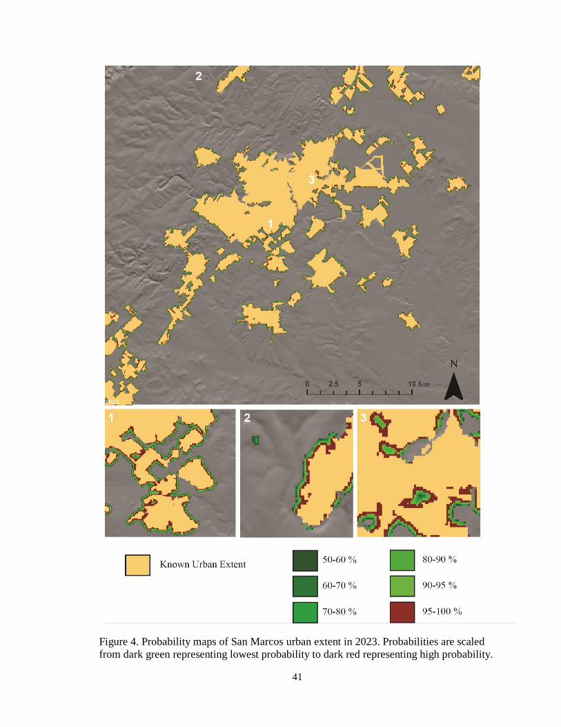
A visual interpretation of the forecasts of urban extent for 2023 (Figure 4)
indicates that the majority of future growth in San Marcos is characterized by edge
growth. Most urban growth is forecasted to occur outward from the city in conjunction
with continued urban infilling between established urban areas. Spontaneous urban
growth is minimal, with only a few pixels representing a relatively low probability of the
occurrence of urban settlement in a new area without pre-existing urban coverage. It is
difficult to interpret the impact of the road growth coefficient in this study area due to a

40
low breed coefficient and with most pre-established urban cores surrounding main road
networks, especially those associated with the highest gravity weighting.
41
Figure 4. Probability maps of San Marcos urban extent in 2023. Probabilities are scaled
from dark green representing lowest probability to dark red representing high probability.

42
5.0 DISCUSSION
5.1 Data and Calibration Modifications
Object-oriented image classification was adequate for classifying urban and non-
urban areas and integration into the model; however, the segmentation of each image
produced slightly different results. While the core of most urban clusters remained
consistent, the segment boundaries of each urban cluster deviated slightly throughout
each image classification. Deviation of urban cluster boundaries is exacerbated with the
Landsat 8 image, likely due to its higher radiometric resolution (12-bit) compared to
Landsat 5 TM (8-bit). Differences in known urban cluster boundaries could be a source
of error during model calibration by creating artificial growth or loss of urban coverage.
To compensate for deviations in urban cluster boundaries each urban extent layers were
merged with the previous year. Thus, each subsequent urban layer will carry over the
maximum urban extent from the previous years. This ensures that all urban clusters are
expanding, eliminates the possibility of urban clusters getting smaller, and makes urban
growth more consistent across all urban extent layers. This operation was not considered
to have a significant impact on the results of the study with the expectation that urban
sprawl in San Marcos has continued to grow rather than shrink during the scope of time
this research has investigated.
SLEUTH implementation suggests resampling input image resolution for both
coarse and fine calibration phases. However, resampling of input image resolution for
these calibration phases had a considerably negative impact on OSM values and
subsequent prediction results. Contrary to results of research by Silva and Clarke (2002),
enhancing the spatial resolution of input images during calibration did not make the

43
model more sensitive to local conditions for this study. Maximum OSM values for final
calibrations using spatially resampled input data with the original and merged urban
extent input layers were 0.341 and 0.382, respectively. Additionally, calibration
coefficients generated through calibration with resampled input images generated urban
predictions with nearly no urban growth. For this study, running all calibration phases
with the full 30 m resolution imagery has produced more meaningful parameter values
for the growth coefficients and urban extent predictions. Wu et al. (2009) opted to use
full resolution for calibration along with other modifications to the model to improve
simulation accuracy.
Poor calibration results from utilizing resampled input images suggest an issue of
scale sensitivity. The drop in calibration performance when using finer resolution
imagery could point towards SLEUTH’s inability to capture the highly dispersed
settlement patterns resulting from local scale factors (Jantz and Goetz 2005, Wu et al.
2009). Alternatively, this maybe due to a relatively short time span (2000-2013) of urban
development used to calibrate the model. Jantz and Goetz (2005) conducted a study using
45 m imagery resampled to 90 m, 180 m, and 360 m to investigate the influence of input
image resolution on the goodness-of-fit between modeled and known urban extent and
the resulting coefficient calibration values. Their description on the behavior of urban
growth for the 45 m spatial resolution shares many similarities with the results of this
study. They found a dominance of edge growth, less dominance in spontaneous new
growth and the spreading of center growth, and minimal development produced through
road growth. Additionally, their results show SLEUTH consistently underestimating the
number of urban edge pixels and urban clusters at a fine input resolution. This may be in

44
part be due to finer resolution data’s inability to fully capture the development patterns of
an urban area, the particular time period chosen for model calibration, or from the
difficulty in evaluating multiple metric-fit statistics (Jantz and Goetz 2005).
OSM values range between zero and one, where an OSM values closer to one
represent a good fit between simulated and known urban extent and the opposite of that
for values closer to zero. Obviously, it is ideal to have high OSM value for each
calibration phase; however, there is no discussion within the literature that identifies a
threshold of OSM values that should be met before initiating an urban growth prediction.
Furthermore, there still remains no general consensus on the most appropriate method to
be used for ranking the best fitting coefficient values. However, Dietzel and Clarke
(2007) assert that the OSM is optimal for evaluating and selecting coefficient parameters
for the best goodness of fit. Alternatively, Wu et al. (2009) suggest performing a
thorough examination of the study area to identify consistent processes and patterns along
with the crucial factors influencing urban growth for a study area. This information can
lend insight into the most appropriate spatial resolution for input images and goodness-
of-fit statistics.
5.2 2023 Forecasted Growth
The forecasts of urban growth made here continue the growth trends from the past
thirteen years. It is clear from the class and landscape metric values and visual outputs of
the model that San Marcos’ urban coverage will continue to expand. The resulting values
of the Clumpiness and Contagion index make sense when considering the prevalence of
forecasted edge growth. Although infilling is projected to occur, the slightly higher
Clumpiness value would suggest that, while the majority of growth would expand
45
outward from urban centers, the 2023 urban extent will not be considerably more or less
aggregated than urban coverage in 2013. Along the same lines with the Contagion Index
value, the slight drop in value between 2013 and 2023 is not considerable enough to
suggest that future urban coverage will be any more fragmented throughout the landscape
than current conditions. Together, these indices indicate that, although growth is expected
to occur, the general shape and distribution of urban sprawl in 2023 will remain similar to
2013.
The high value for the spread coefficient suggests that past growth has been
extending out from the periphery of existing urban clusters. The likelihood of this trend
continuing is further supported by the similarity in the class and landscape metric values
for the Clumpiness and Contagion indices between 2013 and 2023. The coefficient value
for road growth suggests that road networks are influential to urban growth in this study
area. This would make sense as San Marcos is situated as a center point for the
connection to many of the surrounding major highways to IH-35. Despite this, road
influenced urban growth is not visually obvious in the results. Evaluating the effect of
various road weight, or lack thereof, would likely provide more information on the
influence of road weighting on urban growth patterns; however, this was not a focus of
this study.
The low breed and diffusion values indicate that no significant new urban areas
have developed in the area within the past decade and that the expansion of growth from
existing urban areas has been relatively slow. These values are to be expected after
further visual inspection of the urban input layers in which the majority of growth
occurring between each image is through the expansion of currently existing urban areas
46
rather than the development of new areas. Spontaneous growth was almost non-existent
with the exception of a few dark green pixels in the top northwest and south-central
regions of the output image (Number 2 in Figure 4). These small urban areas likely
stayed small due to the low diffusion value. New urban centers may have occurred more
frequently, however, the probability of such growth was not high enough to be displayed
on the output probability map.
It is clear from the results of this study that scale influences coefficient parameters
differently. This issue raises the question of the ability of certain parameters to function
at certain image scales. Jantz and Goetz (2005) found that the highest fit score between
simulated and known urban extents was reached when using the coarsest resolution input
images, although it should be noted their study used different fit metrics from this study.
With the results of this study, a potential for future research would involve investigating
the changes in OSM and coefficient parameter values through calibration using coarser
and finer resolution imagery. Utilization of finer resolution data on a relatively small
study area may help connect modeled and simulated urban extent and reduce the
Clumpiness index. Although this would increase processing time, the results may
produce evidence that confirms or rejects methods of better performance suggested by the
literature.
5.3 SLEUTH Performance
Considering that CA is raster based operation that relies on transitional
neighboring cells to trigger a state change in surrounding cells, it makes sense that the
dominance of urban growth trending towards edge growth in predictions is a common
characteristic of SLEUTH (Jantz and Goetz 2005, Wu et al. 2009). This precedence to

47
edge growth may limit the ability of model to simulate the development of new urban
coverage from other influential factors (Wu et al. 2009). A major point of discussion over
SLEUTH is in its simplicity of urban growth prediction (Chaudhuri and Clarke 2013, Wu
et al. 2009). Principally, SLEUTH is a descriptive model and the transition rules do not
allow for any analysis on the causes of the spatial patterns developed (Santé et al. 2010).
In a real-world situation, there might be various regional developmental plans that could
stimulate a leapfrog urban development throughout the region. Currently, however, the
model is not capable of simulating the potential impacts regional developmental policies
or incentives and the generations of urban extent forecasts are made without the direct
influence of such planning and local-decision making.
The complex emergent behaviors of urban systems are very difficult to model.
All models are abstract representations of this complex and dynamic behaviors and are
flawed to some degree. For the most part, most CA-based urban models are simple in
nature, yet these models are well suited for simulating certain components of the complex
behaviors of urban systems. While SLEUTH is not adapted to the particular urbanism
ideologies that exist in any particular city it is modeling, additional modifications or
coupling with other models may produce results that consider the impact of other factors
influencing growth (Clarke 2008).
SLEUTH is also computationally intensive and can take many hours to days to
complete one of the three calibration phases. Calibration time is dependent on the
calibration phase, cell resolution of input images, the number of coefficient parameters to
be tested, the number of Monet Carlo iterations, and the size of the study area. In this
study, with a relatively small study area and high-resolution input imagery, the combined

48
completion time of all three calibration phases was just over three days. Although
extensive research has gone into developing successful techniques for enhancing the
computational efficiency of calibration (Candau 2000), time of operation continues to be
an issue for SLEUTH (Al-shalabi et al. 2013, Jantz and Goetz 2005, Wu et al. 2009).
49
6.0 CONCLUSION
The results of this study suggest a high probability of continued urban growth
from urban edges with continued aggregation of urban coverage in the gaps between
existing urban areas in 2023. Effective forecasting of growth patterns will be useful tool
in planning decision-making for local municipalities. Based on the results of this study, it
may be recommended that decision makers prepare for aggregation of urban coverage at
the city core with concurrent conversion of available land along the periphery of
established urban areas. Perhaps most beneficial to local planning initiatives would
include information on the predicted locations of newly developed urban centers and the
preference of land use for conversion to urban coverage. This study, however, did not
find any significant probability of such development within the near future or consider
land use conversions.
The results of this study are derived from a standard SLEUTH implementation
with very few model modifications, thus leaving the potential for pursing various avenues
of research for urban modeling of the San Marcos area. These results may be considered
as “business as usual” and could be used as a baseline for comparison to the results of
different predictive scenarios. Other growth scenarios might include environmental
protection parameters, preferential selection of lands for urban growth, or overall
booming urban growth. These scenarios could be initiated through modifications of the
excluded layer or the self-modification parameters and including land use data. Values
for the self-modification parameters were left at the default values for this study. Many
SLEUTH implementations have been conducted in the past, but few have changed their
default values for these parameters (Clarke 2008, Wu et al. 2009). It is possible that
50
modification of these parameters could produce more significant urban growth
predictions and lend insight into the development process of the urban form of a
particular city. This could help local decision-makers evaluate the impact to urban growth
under various city urban planning, resource allocation, and environmental protection
initiatives.
Beyond the results specific to San Marcos, this research has also opened up
research opportunities for the SLEUTH model in general. For the calibration of
coefficient values – if OSM is the best metric to use for the sorting and selection of
values, then perhaps research could be done to investigate a threshold to which OSM
values should not fall below in order to reliably forecast urban growth. Additionally,
investigations on the optimal input image resolutions for various study area sizes would
be beneficial to this study and to anyone interested in conducting a SLEUTH
implementation. With the model’s apparent issues of sensitivity to scale, future research
could be applied towards developing a metric that determines the optimal size of input
cell resolutions that produce coefficient growth values that most closely mimic the urban
development of any particular study area.

51
APPENDIX SECTION
APPENDIX A
Figure 5. 2013 Transportation input image derived from the City of San Marcos’ GIS
Department and U.S. Census TIGER/Line shapefiles.
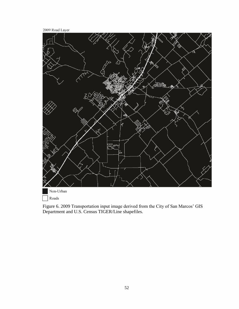
52
Figure 6. 2009 Transportation input image derived from the City of San Marcos’ GIS
Department and U.S. Census TIGER/Line shapefiles.

53
Figure 7. 2004 Transportation input image derived from the City of San Marcos’ GIS Department and U.S. Census TIGER/Line shapefiles.

54
Figure 8. 2000 Transportation input image derived from the City of San Marcos’ GIS
Department and U.S. Census TIGER/Line shapefiles.

55
REFERENCES
Acevedo, William, Timothy W. Foresman, and Janis T. Buchanan. Origins and
philosophy of building a temporal database to examine human transformation
processes. USGS. http://landcover.usgs.gov/urban/umap/pubs/asprs_wma.php
(accessed November 05, 2012).
Anderson, James R., Hardy, Ernest E., and Roach, John T., 1972, A land-use
classification system for use with remote-sensor data: U.S. Geol. Professional Paper
964. USGPO.
Araya, Yikalo H. and Pedro Cabral. 2010. Analysis and modeling of urban land cover
change in Setúbal and Sesimbra, Portugal. Remote Sensing 2, no. 6 (June): 1549-
1563.
Bagan, Hasi and Yoshiki Yamagata. 2012. Landsat analysis of urban growth: How Tokyo
became the world's largest megacity during the last 40years. Remote Sensing of
Environment 127, no. 1 (December): 210-222.
Barredo, José I., Marjo Kasanko, Niall McCormick, and Carlo Lavalle. 2003. Modelling
dynamic spatial processes: Simulation of urban future scenarios through cellular
automata. Landscape and Urban Planning 64, no. 3 (July): 145-160.
Batty, Michael and Yichun Xie. 1994. Modelling inside GIS: Part 2. selecting and
calibrating urban models using ARC-INFO. International Journal of Geographical
Information Systems 8, no. 5 (October): 451-470.
Candau, Jeannette. 2000Caibrating a cellular automaton model of urban growth in a
timely manner. Banff, Alberta, Canada, 4th International conference on Integrating
GIS and Environmental Modeling (GIS/EM4): Problems, Prospects and Research
Needs, September 2-8.
Capital Area Council of Governments. Central Texas regional data.
http://www.capcog.org/ data-maps-and-reports/central-texas-regional-data/ (accessed
October 25, 2012).
———. 2010. CAPCOG Assessment of Growth and Development. Austin, TX: Report
authored by Captial Area Council of Governments.
Chaudhuri, Gargi and Keith C. Clarke. 2013. The SLEUTH land use change model: A
review. The International Journal of Environmental Resource Research 1, no. 1
(January): 88-104.
Cheng, Jianquan and Ian Masser. 2003. Urban growth pattern modeling: A case study of Wuhan City, PR China. Landscape and Urban Planning 62, no. 4 (February): 199-
217.
56
City of San Marcos. Business incentives. http://www.greatersanmarcostx.com/business-
incentives/business-incentives-2 (accessed October 27, 2012).
Clarke, Keith C. 2008. A decade of cellular urban modeling with SLEUTH: Unresolved
issues and problems. Chap. 3, In Planning support systems for cities and regions, ed.
R. K. Brail, 47-60. Cambridge, MA: Lincoln Institute of Land Policy.
Clarke, Keith, Stacy Hoppen, and Leonard Gaydos. 1997. A self-modifying cellular
automaton model of historical urbanization in the San Francisco Bay area.
Environment and Planning B: Planning and Design 24, no. 1 (July): 247-261.
Clarke, Keith C., James A. Brass, and Philip J. Riggan. 1994. A cellular automaton model
of wildfire propagation and extinction. Photogrammetric Engineering & Remote
Sensing 60, no. 11(November): 1355-1367.
Clarke, Keith C. and Leonard Gaydos. 1998. Loose-coupling a cellular automaton model
and GIS: Long-term urban growth predicition for san francisco and
Washington/Baltimore. International Journal of Geographical Information Science
12, no. 7 (August): 699-714.
Clarke, Keith C., Stacy Hoppen, and Leonard Gaydos. 1996. Methods and techniques for
rigorous calibration of a cellular automaton model of urban growth. Santa Fe, New
Mexico, Third International Conference/Workshop on Integrating GIS and
Environmental Modeling, 1996.
Cohen, Barney. 2006. Urbanization in developing countries: Current trends, future
projections, and key challenges for sustainability. Technology in Society 28, no. 1–2
(January-April): 63-80.
Couclelis, H. 1985. Cellular worlds: A framework for modeling micro - macro dynamics.
Environment and Planning A 17, no. 5 (June): 585-596.
Dietzel, Charles and Keith C. Clarke. 2007. Toward optimal calibration of the SLEUTH
land use change model. Transactions in GIS 11, no. 1 (January): 29-45.
Feng, Hui-Hui, Hui-Ping Liu, and Ying Lu. 2012. Scenario prediction and analysis of
urban growth using SLEUTH model. Pedosphere 22, no. 2 (April): 206-216.
García, Andrés M., Inés Santé, Marcos Boullón, and Rafael Crecente. 2012. A
comparative analysis of cellular automata models for simulation of small urban areas
in Galicia, NW Spain. Computers, Environment and Urban Systems 36, no. 4 (July):
291-301.
Geoghegan, J. 2001. Spatially explicit analysis in environmental studies. In International
encyclopedia of the social & behavioral sciences, ed. Editors-in-Chief: Neil J.
Smelser and Paul B. Baltes, 14843-14847. Oxford: Pergamon.

57
Han, Ji, Yoshitsugu Hayashi, Xin Cao, and Hidefumi Imura. 2009. Application of an
integrated system dynamics and cellular automata model for urban growth
assessment: A case study of Shanghai, China. Landscape and Urban Planning 91,
no. 3 (June): 133-141.
Hepinstall-Cymerman, Jeffrey , Stefan Coe, and Marina Alberti. 2009. Using urban
landscape trajectories to develop a multi-temporal land cover database to support
ecological modeling. Remote Sensing 1, no. 4 (December): 1353-1379.
Hickey, Joan Inman. 2011. Learning from the past, planning for the future: A geographic
history of San Marcos, Texas and Texas State University-San Marcos. MS Thesis.
Texas State University - San Marcos.
Jacobson, Carol R. 2011. Identification and quantification of the hydrological impacts of
imperviousness in urban catchments: A review. Journal of Environmental
Management 92, no. 6 (June): 1438-1448.
Jantz, Claire A. and Scott J. Goetz. 2005. Analysis of scale dependencies in an urban
land-use-change model. International Journal of Geographical Information Science
19, no. 2 (February): 217-241.
Jantz, Claire A., Scott J. Goetz, David Donato, and Peter Claggett. 2010. Designing and
implementing a regional urban modeling system using the SLEUTH cellular urban
model. Computers, Environment and Urban Systems 34, no. 1 (January): 1-16.
Jensen, John R. 2005. Introductory digital image processing: A remote sensing
prospective. Upper Saddle River, New Jersey: Prentice Hall.
KantaKumar, Lakshmi N., Nikhil G. Sawant, and Shamita Kumar. 2011. Forecating
urban growth based on GIS, RS, and SLEUTH model in pune metropolitan area.
International Journal of Geomatics & Geosciences 2, no. 2 (November): 568-579.
Kirtland, David, Leonard Gaydos, Keith Clarke, Lee DeCola, William Acevedo, and
Cindy Bell. An analysis of human-induced land transformations in the San Francisco
Bay/ Sacramento area. USGS. http://landcover.usgs.gov/urban/umap/pubs/WRR_
paper.php (accessed November 06, 2012).
Lefsky, M. A., W. B. Cohen, G. G. Parker, and D. J Harding, 2002. Lidar Remote
Sensing for Ecosystem Studies. Bioscience 52, no.1 (January): 19-30.
Li, Yangfan, Xiaodong Zhu, Xiang Sun, and Feng Wang. 2010. Landscape effects of
environmental impact on bay-area wetlands under rapid urban expansion and
development policy: A case study of Lianyungang, China. Landscape and Urban
Planning 94, no. 3-4 (March): 218-227.

58
Liu, Yan. 2009. Modelling urban development with geographical information systems
and cellular automata, 38. Boca Raton, FL: CRC Press.
Lu, D., P. Mausel, M. Batistella, and E. Moran. 2005. Land-cover binary change
detection methods for use in the moist tropical region of the Amazon: A comparative
study. International Journal of Remote Sensing 26, no. 1 (January): 101-114.
Lu, D., P. Mausel, E. BrondÃzio, and E. Moran. 2004. Change detection techniques.
International Journal of Remote Sensing 25, no. 12 (January): 2365-2401.
Mahiny, Abdolrassoul Salman and Keith C. Clarke. 2012. Guiding SLEUTH land-
use/land-cover change modeling using multicriteria evaluation: Towards dynamic
sustainable land-use planning. Environment & Planning B: Planning & Design 39,
no. 5 (September): 925-944.
McGarigal, K., S. A Cushman, and E Ene. 2012. FRAGSTATS v4: Spatial pattern
analysis program for categorical and continuous maps. Computer software program
produced by the authors at the University of Massachusetts, Amherst.
http://www.umass.edu/ landeco/research/fragstats/fragstats.html (accessed December
20, 2012).
Pappas, E. A., D. R. Smith, C. Huang, W. D. Shuster, and J. V. Bonta. 2008. Impervious
surface impacts to runoff and sediment discharge under laboratory rainfall
simulation. Catena 72, no. 1(January): 146-152.
Radhi, Hassan, Fayze Fikry, and Stephen Sharples. 2013. Impacts of urbanisation on the
thermal behaviour of new built up environments: A scoping study of the urban heat
island in bahrain. Landscape and Urban Planning 113, no. 1 (May): 47-61.
Remo, Jonathan W. F., Nicholas Pinter, and Reuben Heine. 2009. The use of retro- and
scenario-modeling to assess effects of 100+ years river of engineering and land-
cover change on middle and lower Mississippi River flood stages. Journal of
Hydrology 376, no. 3–4 (October): 403-416.
Sager, Ryan. Tyler cowen's 10 reasons texas is our future. Time. http://ideas.time.com/
2013/10/ 17/10-reasons-texas-is-our-future/ (accessed Novermber, 05, 2013).
Santé, Inés, Andrés M. García, David Miranda, and Rafael Crecente. 2010. Cellular
automata models for the simulation of real-world urban processes: A review and
analysis. Landscape and Urban Planning 96, no. 2 (May): 108-122.
Scolozzi, Rocco and Davide Geneletti. 2012. A multi-scale qualitative approach to assess
the impact of urbanization on natural habitats and their connectivity. Environmental
Impact Assessment Review 36, no. 1 (September): 9-22.
59
Sezgin, D. and C. Varol. 2012. The effects of urban growth and sprawl on the misuse of
fertile agricultural lands in Ankara. METU Journal of the Faculty of Architecture 29,
no. 1 (January): 273-288.
Shrestha, Milan K., Abigail M. York, Christopher G. Boone, and Sainan Zhang. 2012.
Land fragmentation due to rapid urbanization in the phoenix metropolitan area:
Analyzing the spatiotemporal patterns and drivers. Applied Geography 32, no. 2
(March): 522-531.
Singh, Ashbindu. 1989. Review article digital change detection techniques using
remotely-sensed data. International Journal of Remote Sensing 10, no. 6 (July): 989-
1003.
Silva, Elisabete A., Jack Ahern, and Jack Wileden. 2008. Strategies for landscape
ecology: An application using cellular automata models. Progress in Planning 70,
no. 4 (November): 133-177.
Silva, Elisabete A. and Keith C. Clarke. 2002. Calibration of the SLEUTH urban growth
model for lisbon and porto, portugal. Computers, Environment and Urban Systems
26, no. 6 (November): 525-552.
Soltész, Kinga. 2010. Sustainable urban development and developing countries. Juridical
Current 13, no. 4 (December): 144-152.
Tewolde, Mussie G. and Pedro Cabral. 2011. Urban sprawl analysis and modeling in
Asmara, Eritrea. Remote Sensing 3, no. 1 (September): 2148-2165.
Texas Comptroller of Public Accounts. Texas in focus: A statewide view of
opportunities. Texas Comptroller of Public Accounts. http://www.window.state.
tx.us/specialrpt/tif/population.html (accessed November, 05, 2013).
Texas State University (TXSU).Campus construction. http://www.fss.txstate.edu/
planning/fac_pln/construction.html (accessed November 02, 2012).
———. Factbook pivot table: Census day enrollment. http://www.ir.txstate.edu/
Facts/xfacts.html (accessed November 05, 2012).
Tobler, W. R. 1979. Cellular Geography. In Philosophy in Geography, ed. S. Gale and G.
Olsson, 379-386. Dordrecht, Holland: D. Reidel Publishing Company.
U.S. Bureau of the Census. American FactFinder. U.S. Bureau of the Census.
http://factfinder2.census.gov/faces/nav/jsf/pages/index.xhtml (accessed November
13, 2012).
60
U.S Department of Transportation Federal Highway Administration. FHWA functional
classification guidelines. http://www.fhwa.dot.gov/planning/processes/statewide/
related/highway_functional_classifications/section02.cfm (accessed November, 05,
2013).
United Nations, Department of Economic and Social Affairs, Population Division. 2012.
World urbanization prospects, the 2011 revision: highlights. United Nations, New
York.
———. 2011. Population distribution, urbanization, internal migration and
development: An international perspective. United Nations, New York.
Univeristy of Texas - Austin (UT). The University of Texas at Austin releases
preliminary enrollment data. http://www.utexas.edu/news/2012/09/19/2012-
preliminary-enrollment-data/ (accessed January 15, 2013).
University of California Santa Barbara (UCSB). Project Gigalopolis.
http://www.ncgia.ucsb.edu/projects/gig/index.html (accessed September 30, 2012).
White, Michael D. and Keith A. Greer. 2006. The effects of watershed urbanization on
the stream hydrology and riparian vegetation of los peñasquitos creek, california.
Landscape and Urban Planning 74, no. 2 (January): 125-138.
Wolfram, Stephen. 1984. Cellular automata as models of complexity. Nature 311, no. 1
(October): 419-424.
Wu, Xiaoqing, Yuanman Hu, S. He Hong, Rencang Bu, Jeff Onsted, and Fengming Xi.
2009. Performance evaluation of the SLEUTH model in the shenyang metropolitan
area of northeastern china. Environmental Modeling & Assessment 14, no.2 (May):
221-230.
Yang, Xiaojun. 2002. Satellite monitoring of urban spatial growth in the Atlanta
metropolitan area. Photogrammetric Engineering & Remote Sensing 68, no.7 (July):
725-734.
Yeh, Anthony Gar-On and Xia Li. 2001. Measurement and monitoring of urban sprawl in
a rapidly growing region using entropy. Photogrammetric Engineering & Remote
Sensing 67, no. 1 (January): 83-90.
Zhang, Chi, Hanqin Tian, Guangsheng Chen, Arthur Chappelka, Xiaofeng Xu, Wei Ren,
Dafeng Hui, et al. 2012. Impacts of urbanization on carbon balance in terrestrial
ecosystems of the southern United States. Environmental Pollution 164, no. 1 (May):
89-101.

61
Zhao, Shuqing, Liangjun Da, Zhiyao Tang, Hejun Fang, Kun Song, and Jingyun Fang.
2006. Ecological consequences of rapid urban expansion: Shanghai, China.
Frontiers in Ecology and the Environment 4, no. 7 (September): 341-346.
Zhou, Qiming, Baolin Li, and Yumin Chen. 2011. Remote sensing change detection and
process analysis of long-term land use change and human impacts. AMBIO - A
Journal of the Human Environment 40, no. 7 (November): 807-818.