Modeling of rheological properties for entangled polymer

Scholars' Mine

Doctoral Dissertations Student Theses and Dissertations

Spring 2016

Modeling of rheological properties for entangledpolymer systemsNilanjana Banerjee

Follow this and additional works at: https://scholarsmine.mst.edu/doctoral_dissertations

Part of the Chemical Engineering CommonsDepartment: Chemical and Biochemical Engineering

This Dissertation - Open Access is brought to you for free and open access by Scholars' Mine. It has been accepted for inclusion in DoctoralDissertations by an authorized administrator of Scholars' Mine. This work is protected by U. S. Copyright Law. Unauthorized use includingreproduction for redistribution requires the permission of the copyright holder. For more information, please contact [email protected].

Recommended CitationBanerjee, Nilanjana, "Modeling of rheological properties for entangled polymer systems" (2016). Doctoral Dissertations. 2468.https://scholarsmine.mst.edu/doctoral_dissertations/2468

http://www.mst.edu/?utm_source=scholarsmine.mst.edu%2Fdoctoral_dissertations%2F2468&utm_medium=PDF&utm_campaign=PDFCoverPages

http://www.mst.edu/?utm_source=scholarsmine.mst.edu%2Fdoctoral_dissertations%2F2468&utm_medium=PDF&utm_campaign=PDFCoverPages

https://scholarsmine.mst.edu?utm_source=scholarsmine.mst.edu%2Fdoctoral_dissertations%2F2468&utm_medium=PDF&utm_campaign=PDFCoverPages

https://scholarsmine.mst.edu/doctoral_dissertations?utm_source=scholarsmine.mst.edu%2Fdoctoral_dissertations%2F2468&utm_medium=PDF&utm_campaign=PDFCoverPages

https://scholarsmine.mst.edu/student-tds?utm_source=scholarsmine.mst.edu%2Fdoctoral_dissertations%2F2468&utm_medium=PDF&utm_campaign=PDFCoverPages

https://scholarsmine.mst.edu/doctoral_dissertations?utm_source=scholarsmine.mst.edu%2Fdoctoral_dissertations%2F2468&utm_medium=PDF&utm_campaign=PDFCoverPages

http://network.bepress.com/hgg/discipline/240?utm_source=scholarsmine.mst.edu%2Fdoctoral_dissertations%2F2468&utm_medium=PDF&utm_campaign=PDFCoverPages

https://scholarsmine.mst.edu/doctoral_dissertations/2468?utm_source=scholarsmine.mst.edu%2Fdoctoral_dissertations%2F2468&utm_medium=PDF&utm_campaign=PDFCoverPages

mailto:[email protected]

MODELING OF RHEOLOGICAL PROPERTIES FOR ENTANGLED

POLYMER SYSTEMS

by

NILANJANA BANERJEE

A DISSERTATION

Presented to the Faculty of the Graduate School of the

MISSOURI UNIVERSITY OF SCIENCE AND TECHNOLOGY

In Partial Fulfillment of the Requirements for the Degree

DOCTOR OF PHILOSOPHY

in

CHEMICAL ENGINEERING

2016

Approved by

Joontaek Park, Advisor

Parthasakha Neogi

Jee-Ching Wang

Dipak Barua

V. A. Samaranayake

2016

NILANJANA BANERJEE

All Rights Reserved

iii

PUBLICATION DISSERTATION OPTION

This dissertation consists of the following three articles that have been

published/submitted for publication as follows:

Paper I, pages 37-79 have been published in KOREAN JOURNAL OF CHEMICAL

ENGINEERING.

Paper II, pages 80-145 have been published in JOURNAL OF RHEOLOGY.

Paper III, pages 146-188 have been submitted for publication in JOURNAL OF

RHEOLOGY. Appendices A and B have been added for purposes normal to dissertation

writing.

iv

ABSTRACT

The study of entangled polymer rheology both in the field of medicine and polymer

processing has their major importance. Mechanical properties of biomolecules are studied

in order to better understand cellular behavior. Similarly, industrial processing of polymers

needs thorough understanding of rheology so as to improve process techniques. Work in

this dissertation has been organized into three major sections. Firstly, numerical/analytical

models are reviewed for describing rheological properties and mechanical behaviors of

cytoskeleton. The cytoskeleton models are classified into categories according to the length

scales of the phenomena of interest. The main principles and characteristics of each model

are summarized and discussed by comparison with each other, thus providing a systematic

understanding of biopolymer network modeling. Secondly, a new constitutive “toy” Mead-

Banerjee-Park (MBP) model is developed for monodisperse entangled polymer systems,

by introducing the idea of a configuration dependent friction coefficient (CDFC) and

entanglement dynamics (ED) into the MLD “toy” model. The model is tested against

experimental data in steady and transient extensional and shear flows. The model

simultaneously captures the monotonic thinning of the extensional flow curve of

polystyrene (PS) melts and the extension hardening found in PS solutions. Thirdly, the

monodisperse MBP model is accordingly modified into polydisperse MBP “toy”

constitutive model to predict the nonlinear viscoelastic material properties of model

polydisperse systems. The polydisperse MBP toy model accurately predicts the material

properties in the forward direction for transient uniaxial extension and transient shear flow.

v

ACKNOWLEDGEMENTS

The accolade for the success of this research project is not alone mine, rather it goes

to a lot of people who have been there behind the scene but have equally played an

important role to make this endeavor a success.

First and foremost, I thank God for giving me the strength and guidance to do things

in the right way.

My heartfelt gratitude and thanks goes to my advisor Dr. Joontaek Park, without

whom, even the smallest of the steps towards the completion of these projects would not

have been possible. His help and support has made it possible for me to do whatever I have

accomplished. His continuous encouragement has allowed me to overcome my obstacles.

His guiding hands have taught me to think and work as a better engineer.

Special thanks to my committee members, Dr. Parthasakha Neogi, Dr. V. A.

Samaranayake, Dr. J. C. Wang and Dr. Dipak Barua, without whose support, fulfillment of

this dissertation would not have been possible.

A big hug, thanks and lots of love for my parents and my sister Payal, for being my

support. For keeping the trust in me and for believing in my capabilities.

Last but not the least, I thank Missouri University of Science and Technology for

giving me a forum to enhance my knowledge and learn to become a professional. Thanks

to the institute also for giving me innumerable memories to be cherished throughout my

life.

vi

TABLE OF CONTENTS

Page

PUBLICATION DISSERTATION OPTION…………………………………………. iii

ABSTRACT……………………………………………………………………............ iv

ACKNOWLEDGEMENTS…………………………………………………................. v

LIST OF ILLUSTRATIONS………………………………………………................... xi

LIST OF TABLES………………………………………………………….................. xv

NOMENCLATURE………………………………………………………………....... xvi

SECTION

1. INTRODUCTION…………………………………………………………… 1

1.1. OVERVIEW………………………………………………….………. 1

1.2. MODELING AND SIMULATION OF BIOPOLYMER

NETWORKS: CLASSIFYING THE CYTOSKELETON MODELS

ACCORDING TO MULTIPLE SCALES ……………………………. 2

1.2.1. Research Motivation………………….….…………………... 2

1.2.2. Research Objectives…………………………………….….... 4

2. CONSTITUTIVE MODELS FOR MONODISPERSE AND

POLYDISPERSE ENTAGLED POLYMER SYSTEMS …………………… 6

2.1. RESEARCH MOTIVATION………………….………………….….. 6

2.2. RESEARCH OBJECTIVES………………………………………….. 8

2.3. INTRODUCTION TO DOI AND EDWARDS’ TUBE THEORY…… 9

2.3.1. Doi and Edwards’ Tube Theory…………………………….... 9

2.3.2. Polymer Relaxation Mechanism………………………….….. 18

vii

3. HISTORY OF MONODISPERSE SYSTEM CONSTITUTIVE “TOY”

MODEL DEVELOPMENT….…………………………………………...…. 24

4. HISTORY OF POLYDISPERSE SYSTEM CONSTITUTIVE “TOY”

MODEL DEVELOPMENT……………………………………………......... 32

PAPER

I. Modeling and simulation of biopolymer networks: Classification of the

cytoskeleton models according to multiple scales………................................. 37

Abstract…………………………………………………………….… 37

INTRODUCTION………………………………………………….… 38

CELL-SCALE CONTINUUM-BASED MODELS (~10 m) ………. 43

1. Elastic/Viscoelastic Models…………………………………. 43

2. Multiphasic Model……………………………………......…. 44

3. Soft Gassy Models…………………………………….….…. 45

4. Discussion of the Cell-Scale Continuum-based Models….…. 46

STRUCTURE-BASED MODEL (1~10 m) ……………………...… 48

1. Cortical Membrane Model………………….……….…......... 49

2. Tensed Cable Nets Models………………………………...... 49

3. Tensegrity (Cable-strut) Models…………………………….. 50

4. Open Cell Foam Model……………………………………… 52

5. Semi-flexible Network Element Model…………………....... 52

6. Continuum Polymer Network Model……………………....... 53

7. Discussion on the Structure-based Models………………....... 54

POLYMER-BASED MODELS (<1 m) …………………………..... 56

1. Discrete Network Models………………………….……........ 57

2. Single Polymer Chain Model……………………………....... 59

viii

3. Discussion on the Polymer-based Models………………....... 60

DISCUSSION/SUMMARY…………………………….……….…… 62

CONCLUDING REMARKS……………………………….……........ 65

ACKNOWLEDGEMENT …………………………………………… 71

REFERENCES…………………………………………………….…. 72

II. A constitutive model for entangled polymers incorporating binary

entanglement pair dynamics and a configuration dependent friction

coefficient………………………..................................................................... 80

Synopsis…………………………………………………………........ 80

I. INTRODUCTION……………………………………………………. 82

II. MODELLING THE ENTANGLEMENT PAIR DYNAMICS FOR

MONODISPERSE SYSTEMS………………………………………. 85

A. Formulation of the expression for Kuhn bond based CDFC on

the stretch and terminal orientational relaxation times ………. 91

III. MODIFICATION OF THE DESAI-LARSON TOY DEMG MODEL

TO INCORPORATE ED, CDFC, AND CCR ………………………... 94

IV. MODIFICATION OF THE NEW CDFC-ED TOY MLD MODEL TO

ACCOUNT FOR REDUCED LEVELS OF CCR FOR HIGHLY

ALIGNED SYSTEMS …………………………………………….…. 96

V. SUMMARY OF THE EQUATIONS IN THE EDS - KUHN BOND

CDFC REFORMULATION OF THE MONODISPERSE MLD TOY

MODEL ……………………………………………………………… 99

VI. SIMULATION OF MONODISPERSE LINEAR PS MELTS AND

ENTANGLED SEMIDILUTE SOLUTIONS IN STEADY AND

TRANSIENT UNIAXIAL EXTENSION …………………………… 102

A. Simulation of monodisperse linear PS melts and solutions in

steady and transient shear flow ……………………………… 109

VII. DISCUSSION/SUMMARY………………………………….….…… 111

ACKNOWLEDGMENTS …………………………...……………………… 128

ix

APPENDICES

A. DERIVATION ………………………………………….…… 129

B. GENERALIZATION OF THE NEW EDS – CDFC MLD

TOY MODEL TO POLYDISPERSE SYSTEMS …………... 131

C. INTERNAL DETAILS OF THE MODEL CALCULATIONS 137

References………………………………...…………………………………. 141

III. Constitutive model for polydisperse entangled polymers incorporating binary

entanglement pair dynamics and a configuration dependent friction

coefficient…………….……………………….…………………………....... 146

Synopsis…………………………………….………………………… 146

I. INTRODUCTION……………………………………………………. 147

II. THE POLYDISPERSE MBP “TOY” MODEL FOR LINEAR

POLYMERS …………………………………………………………. 150

A. Incorporation of dilute tube theory into the monodisperse

MBP model ……………………….…………...……….......... 150

B. Summary of the polydisperse MBP “toy” model equations….. 153

C. Numerical simulation……………………….……….………. 157

III. COMPARISON TO EXPERIMENTAL DATA …………………….. 158

A. Uniaxial extension flow of polydisperse PS melts and

solutions……………………………………….….…….…… 158

B. Shear flow of polydisperse PS melts and solutions……….…. 160

IV. INVESTIGATION ON THE EFFECT OF POLYDISPERSITY ……. 161

V. CONCLUSION ……………………………………………….……… 164

References…………………………………………………………....…….... 185

SECTION

5. CONCLUSION……………………………………….………………...…… 189

x

APPENDICES

A. TRACE OF ORIENTATION TENSOR ( tSijtube,

) FOR THE MBP

POLYDISPERSE “TOY” MODEL ………………………………...... 196

B. ADDITIONAL FIGURES AND TABLES FOR THE MBP

POLYDISPERSE “TOY” MODEL ………………………………...... 198

REFERENCES ……………………………………………………………………... 213

VITA…………………………………………………….…………………….……. 219

xi

LIST OF ILLUSTRATIONS

Figure Page

SECTION

1.1. Classification of the cytoskeleton mechanics models and their underlying

principles………………………………………………………………....... 3

1.2. Classification of the cytoskeleton mechanics model based on length and

time scales……………………………………………………………..…... 4

2.1. The steady state extensional viscosity vs extension rate for 200K PS melt

and 20w% 1.95M PS solution respectively………………………….…….. 8

2.2. An entangled polymer system with the primary chain (bold black) with its

entanglements (green) and constraints by other chains around it………..…. 12

2.3. A virtual tube (green color) of radius a, created along the contour length of

the primitive chain is the sum of the constraints around it.…………….…... 13

2.4. Reptative motion of the chain out of a tube causes simultaneous tube

creation and destruction along the chain contour length……………..…….. 17

2.5. Characteristic relaxation times………………………………………..…… 18

2.6. Primitive path fluctuation mechanism………………………………..……. 20

2.7. Constraint release mechanism………………………………………..……. 23

3.1. Steady shear viscosity vs shear rate curve showing DEMG, MLD and

experimental results for 200KPS monodisperse melt……………..……….. 28

3.2. Steady extensional viscosity vs extension rate curve showing DEMG,

MLD and experimental results for 200KPS monodisperse melt……..…….. 29

4.1. Nested tube model proposed by Auhl et al. (2009) ………………….…….. 34

4.2. Diluted stretch tube model proposed by Mishler & Mead 2013a………..…. 35

PAPER I

1. Schematic diagram which shows the structural components of the

cytoskeleton in a typical eukaryotic cell and the length scales for each

group of models………………………………………………………….… 66

xii

2. A typical example of 2D tensed cable nets models: reinforced squared

nets……………………………………………………………………….... 66

3. A typical octahedron tensegrity element structure……………………..…... 67

4. The RVEs of (a) a typical open cell foam model (cuboid), (b) the semi-

flexible polymer network model, and (c) the continuum polymer network

models (8-chain model) ………………………………………………........ 67

PAPER II

1. Schematic diagram for tube shortening when 1tube

S : The tube is crinkled

and constraint release shortens the tube and relaxes stretch and orientation

[Mead et al. (1998), Mead (2011a)]…………………..…………………..... 115

2. Schematic diagram for tube shortening when 1tube

S : Constraint release

does not relax any stretch……………………………….…………………. 115

3. Steady state extensional viscosity as a function of extension rate:

Experimental data is for monodisperse PS200K at 130oC [Bach et al.

(2003)]……………………………………………………..………………. 116

4. The steady state entanglement density, N , versus extension rate, , for

the MBP model and the MBP-xccr model …………………………………. 117

5. The relative stretches for MBP, MBP-xccr, and DEMG-cdfc……………… 118

6. Transient extensional viscosity, 𝜂𝑒(𝑡) versus t, for monodisperse PS200K

at an extension rate of 0.01 sec-1 (𝜀𝜏𝑠,𝑒𝑞 ≈ 1)……………………………… 119

7. Normalized stress relaxation after imposing 3 Hencky strain units for a

monodisperse PS145K melt at 120oC at three different steady extension

rates………………………………………………………..……………..... 120

8. Steady state extensional viscosity as a function of extension rate.…………. 121

9. Steady state extensional viscosity as a function of extension rate………….. 122

10. The (slope of shear stress-shear rate curve) derivative of steady shear stress

with respect to ��, 𝑑𝜎𝑥𝑦

𝑑�� versus �� for a family of β values……………...……. 123

11. The shear flow curve, vs. , for a monodisperse PS solution 7% 8.42M

PS…………………………………………………………………...……... 124

xiii

12. The first normal stress difference for a monodisperse PS solution 7%

8.42M PS is shown, 1N vs. ……………………………………………… 125

13. Transient monodisperse 200K-S PS melt at shear rates of 1s-1, 10s-1 and

30s-1……………………………………………………..………………..... 126

PAPER III

1. Qualitative sketch of the orientational and stretch relaxation spectra for two

hypothetical molecular weight distributions…………………….…………. 166

2. Sketch of a typical broad MWD for a commercial polymer system with

orientational and stretch relaxation spectra overlap………………..………. 167

3. Sketch of the three distinct unraveled “tubes” used in the polydisperse MBP

model and their interrelationships……………………………………...….. 168

4. Transient extensional viscosity curves for PSM2 (see Table III for the

data) at 𝜀 =0.013, 0.097, and 0.572s-1………………………………...……. 169

5. Transient extensional viscosity curves for PSM1 (see Table II for the

data) at 𝜀 =0.00015, 0.01, and 0.3 s-1……………………………………..... 170

6. Transient extensional viscosity curves for PSM1 (see Table II for the

data) at 𝜀 =0.3 s-1………………………………………………………...…. 171

7. Transient extensional viscosities for PSS1 (see Table II for the data) at

𝜀 =0.5 and 1.0 s-1………………………………………………………...…. 172

8. Transient shear viscosities for 7% PS blend solution (PSS2 see Table V

for details) at 𝛾 0.01, 0.1 and 100 sec-1………………………………...….. 173

9. Transient normal stress differences for 7% PS blend solution (PSS2 see

Table V for details) at 𝛾 0.01, 0.1 and 100 sec-1…………………………..... 174

10. Transient shear viscosity for PS melt (PSM3) (PI = 3.2) (see Table VI for

details) at 𝛾 0.05 and 2.0 sec-1 respectively……………………………….... 175

11. Transient uniaxial extensional viscosity curves of each polymer component

for PS bidisperse melt, PSM1 [Read et al. (2012)], at ��=0.00015, 0.01 and

0.3 s-1, predicted by MBP model……………………………………….…... 176

12. Transient fractional stretch, x(t)=Λ(t)/Λmax, curves of each polymer

component for PS bidisperse melt, PSM1 [Read et al. (2012)], at

𝜀 =0.00015, 0.01 and 0.3 s-1, predicted by MBP model……………………... 177

xiv

13. Transient relative stretch, Λ(t)=L(t)/Leq(t), curves of each polymer

component for PS bidisperse melt, PSM1 [Read et al. (2012)], at

𝜀 =0.00015, 0.01 and 0.3 s-1, predicted by MBP model……………………... 178

14. Transient normalized entanglement dynamics curves of each entanglement

pair for PS bidisperse melt, PSM1 [Read et al. (2012)], at ��=0.00015, 0.01

and 0.3 s-1, predicted by MBP model……………………………………..... 179

15. Transient relative stretch curves for Wesslau’s log-normal MWD, for

components 1, 4, 7, and 10, at ��=10 s-1, predicted by MBP model………..... 180

SECTION

5.1. Analytic rheology scheme…………………………………………………. 194

xv

LIST OF TABLES

Table Page

PAPER I

1. Summary of the cytoskeleton models……………………………………. 68

PAPER II

I. Summary of the family of “toy” molecular models studied……………… 127

II. Experimental data sets compared………………………………………... 127

PAPER III

I. Summary of the experimental data sets used in this study………………. 181

II. Simulation input values for the uniaxial extension of bidisperse PS melt

with PI = 1.248 (PSM1) [Read et al., (2012)] and bidisperse 7% PS

solution (PSS1) [Ye et al., (2003)]………………………………………. 181

III. Simulation input values for the data set PSM2 (PS 686 spiked with MW

3.2×106 component; PI=2.33) directly taken from [Mishler and Mead

(2013b)], which was originally obtained from Minegishi et al…………... 182

IV. Summary of which physical effects are included/excluded in each model,

compared in Figure 5…………………………………………………….. 183

V. Simulation input values for shear 7% bidisperse PS solution (PSS2)

[Pattamaprom and Larson (2001)]………………………………………. 183

VI. Simulation input values for shear PSM3 [PS melt (P1) (PI=3.5)] [Ye and

Sridhar (2005)]…………………………………………………………... 183

VII. Simulation input values for model generated Wesslau’s log-normal PS

melt MWD with PI = 2.33 and weight avg. MW =2.4 105 (PSMW)……. 184

xvi

NOMENCLATURE

Symbol Description

C∞ Characteristic ratio of the polymer

GN0 Equilibrium plateau modulus of fully entangled chain

GN(t) Dynamic plateau modulus of partially disentangled chain

Iij Tension induced orientation tensor

J Number of C-C sigma bonds in the backbone of polymer monomer

kid Non-linear spring constant for diluted tube

ks / ksi Non-linear spring constant

L(t) Current tube contour length

Leq Initial equilibrium length

Leq(t) Current equilibrium length

M/Mi Molecular weight of component

Mc Critical molecular weight

Me Entanglement molecular weight

Me(t) Entanglement molecular weight of partially disentangled chain

Mn Number average molecular weight

Mo Molecular weight of a single monomer of the polymer system

n Number of Kuhn bonds in an entanglement segment

N(t) Rate of change of number of entanglements on a chain

N(t) / Nij(t) Number of entanglements on a partially disentangled chain

xvii

Ne /Nij0 Average equilibrium number of entanglements per chain

R Unit end-to-end vector of a tube segment

Skuhn Net Kuhn bond orientation

Sid Orientation tensor of the diluted tube

Stube Orientation tensor

Stubeij Tube segment orientation of the ijth entanglement pair

Stube/Stubei Single tube segment orientation

Sxx, Syy, Sxy Tube segment orientation in x, y and xy direction.

wi / wj Weight fraction of the ith / jth component in MWD

x / xi Fractional extension of the chain

xid Fractional extension of the diluted tube

Greek nomenclature

α / αi Ratio between the maximum stretch ratios of relative stretches

��(𝑡)/αi (t) Rate of change of the maximum stretch ratios

αid (t) / αid α values for diluted tube

β Entanglement dynamics efficiency

ϵ and γ Extension rate and shear rate respectively

ζ(t) Friction factor

ζeq Equilibrium friction factor

ηe and η Extensional viscosity and shear viscosity respectively

κ Velocity gradient

λ(t) Relative stretch of a fully entangled chain

xviii

λmax Maximum relative stretch of a fully entangled chain

Λ / Λ(t) Relative stretch of partially disentangled chain

Λ(𝑡)/Λi (t) Rate of change of relative stretch

Λid Relative stretch of the diluted tube

Λmaxid Maximum relative stretch of the diluted tube

Λmax(t) Maximum relative stretch of the chain as a function of ED

τd0 Equilibrium reptation / disengagement / orientation time

𝜏𝑑(𝑡)/τdi(t) Reptation / disengagement / orientation time

τdij Reptation / orientation time of ijth entanglement pair

τs0 Equilibrium longest rouse / stretch relaxation time

𝜏𝑠(𝑡)/τsi(t) Longest rouse / stretch relaxation time

τsieff Effective rouse time for the diluted tube

σxx-yy(t) Extensional Stress or Normal stress difference in case of shear flow

σxy(t) Shear stress

φp Weight fraction (solution or melt)

Φ Fractional rate of matrix entanglement renewal

ψi Fractional dilution level of the ith component of the MWD

Abbreviations

CCR Convective constraint release

CDFC Configuration dependent friction coefficient

CR Constraint release

DE Doi and Edwards model

xix

DEMG Doi – Edwards – Marrucci – Grizzuti model

ED Entanglement dynamics

LCB Long chain branched polymer

LVE Linear viscoelastic envelope

MBP Mead – Banerjee – Park model

MFI Melt flow index

MLD Mead – Larson – Doi model

MW Molecular weight

MWD Molecular weight distribution

PI Polydispersity index and/or Polyisoprene (refer to context)

PS Polystyrene

RVE Representative volume element

1

1. INTRODUCTION

1.1 OVERVIEW

Studies of entangled polymer systems have been underway for a long time both in

the field of biological sciences and commercial polymer industries. The macromolecules,

like proteins, and more complex structures, like cytoskeletons and external cellular matrix,

have been under exploration in order to understand cellular behavior and diseases more

thoroughly. Similarly, the rheological behavior of commercial polymer macromolecules,

both linear and linear branched chains, is important to understand, as they are exposed to

high shear and extension deformation conditions during industrial processing. Better

understanding of the mechanical properties of these polymers allows better process design

and material handling. The discussion in subsequent sections, is categorized in three major

parts. Paper I consists of the classification of the cytoskeleton models according to multiple

scales. The discussion in Papers II and III are dedicated to the development of constitutive

“toy” models for both monodisperse and polydisperse entangled polymer systems

respectively.

The discussion in the section below has been organized as follows. In Section 1.2,

the motivation and objectives behind the research topic “modeling and simulation of

biopolymer network classification of the cytoskeleton models according to multiple scales”

are discussed. A very brief glance at how the classification of models has been organized

is also included. Section 2 is dedicated to discussing the constitutive models for

monodisperse and polydisperse entangled polymer systems. The Section 2 is further

categorized into sub sections as follows. In Sections 2.1 and 2.2, the motivation and the

2

objectives behind the research respectively are discussed. The constitutive models for the

monodisperse and polydisperse systems are a modification of the Doi-Edwards’ “tube

model.” Thus, a brief introduction to the tube theory and basic polymer relaxation

mechanism is imperative before moving forward with the model development, which is

taken up in Section 2.3. In Sections 3 and 4 the history of the mathematical models that

have been developed over time to describe the rheology of entangled monodisperse and

polydisperse polymer systems are respectively discussed.

1.2. MODELING AND SIMULATION OF BIOPOLYMER NETWORKS:

CLASSIFYING THE CYTOSKELETON MODELS ACCORDING TO

MULTIPLE SCALES

Cytoskeleton mechanics and the field of biomechanics have been topics of research

for last couple of decades, as they are pathways to explain various cellular behaviors and

also answer certain pertinent questions regarding recent diseases like cancer, tumour

growth, neural degeneration, etc. The cytoskeleton, which is the structure providing

component of the cell, changes its behavior under different mechanical conditions,

changing the cellular activity accordingly. The questions here are what happens to the

cytoskeleton structure under a certain mechanical perturbation and what are the reasons

behind the observed deformations. The understanding of the above questions can be

extended to answering what happens to the cellular activity under the deformation of the

cytoskeleton (Banerjee & Park, 2015).

1.2.1. Research Motivation. The questions regarding the cytoskeleton

mechanical behavior and properties and their answers have been one of the major

3

motivations behind studying this particular topic. From the onset of the research, it was

clear that numerous mathematical models to describe the behavior of the cytoskeleton

structure exist. The range of the models was extremely varied from that of viscoelastic to

glassy material to that of a Brownian dynamic simulation of a discrete polymer network

system. Many attempts have been made to provide a clear demarcation between the various

models and their results (Banerjee & Park, 2015), but there is a lack of review articles that

bring in all the various models together and put forward a clear picture of how and why the

models are different. This was the second major motivation to bring together a review

article that could bring all the present mathematical models together, explain their

differences and provide a literature structure for future research in this field (Banerjee &

Park, 2015).

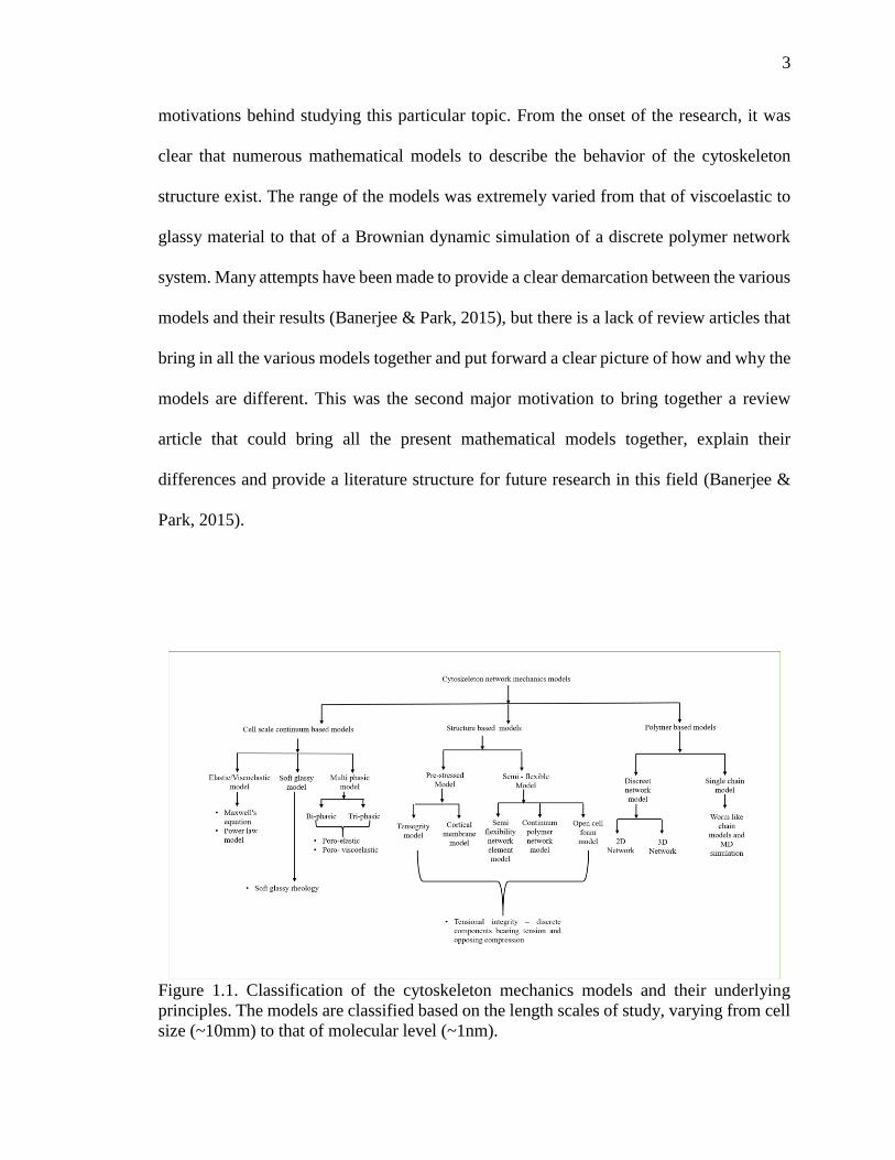
Figure 1.1. Classification of the cytoskeleton mechanics models and their underlying

principles. The models are classified based on the length scales of study, varying from cell

size (~10mm) to that of molecular level (~1nm).

4

Figure 1.2. Classification of the cytoskeleton mechanics model based on both length and

time scales. It can be clearly seen that the chosen time and length scales cause drastic

difference in the model consideration for cytoskeleton rheological study.

1.2.2. Research Objectives. The objectives behind the research are as follows

(Banerjee & Park, 2015):

1. This research was intended to provide a systematic understanding of

cytoskeleton models in terms of length scales, which, in turn, affects the mechanical

stress behavior of the cytoskeleton. Figures 1.1. and 1.2. provide a brief description

of the classification of the models based on the length and time scales. It can be

seen that depending on the chosen length scale or the time scale of the cytoskeleton

mechanics model, the rheological behavior being described changes.

2. The final objective was to provide a framework for the future development

of the cytoskeleton mechanical models.

5

3. This research was designed to assimilate all major recently published

mathematical models and provide a summary of their underlying principles, main

applications, and advantages and disadvantages.

The detailed discussion regarding the classifications, the underlying mechanism,

and their pros and cons appears in Paper I, in the later part of the dissertation.

6

2. CONSTITUTIVE MODELS FOR MONODISPERSE AND POLYDISPERSE

ENTANGLED POLYMER SYSTEMS

Nonlinear rheological behavioral studies of both entangled polymer melts and

solutions (both monodisperse and polydisperse) under high deformation conditions have

been underway for more than half a century. The tube theory developed by Doi and

Edwards in 1986 provided a platform that has been modified and re-modified numerous

times to date, generating different models, but has been unable to provide a single unified

approach to describe the system as a whole (Doi & Edwards, 1986). Simultaneously there

have been molecular dynamics simulation, stochastic Brownian dynamics approaches to

study the same system of polymer under low and high deformation conditions (Park et al.,

2012; Xu et al., 2006).

2.1. RESEARCH MOTIVATION

One of the major motivations behind this particular research has been to provide a

generalized “toy” constitutive model that correctly and consistently describes all the

physics behind the rheological behavior of the entangled polymer in a fast flow nonlinear

regime. The system in this study was restricted to only that of polystyrene (PS) melts and

solutions. The conclusions drawn from the same study can easily be transcribed to any

other polymer systems (Mead et al., 2015).

Secondly, a strong physical basis was sought in order to describe the nonlinear

rheological behavior for both the monodisperse polymer melt and solution systems.

Experimental observations demonstrated that under high extension rates, monodisperse

polymer melts exhibit an extension thinning behavior. Figure 2.1., which describes the

7

steady state extension curve for 200K PS melt w.r.t extension rates (Mead et al., 2015)).

The physics behind it is not yet understood. There have been quite a few developments in

the field to aid in understanding the reason behind it, but the results have been inconclusive.

The approach used in the study was to find the underlying physics to describe this behavior.

Thirdly, monodisperse entangled polymer melt and polymer solution behave

differently under similar extension conditions (see Figure 2.1., which provides a

comparison between the steady state extensional viscosity behavior of 200K PS melt and

20wt% 1.95M PS solution w.r.t extension rate (Mead et al., 2015)). The entangled polymer

melt shows extension thinning behavior, and the polymer solution shows extension

thickening, under similar high extension conditions. There was also a desire to determine

whether the constitutive “toy” model could both capture and explain the reasons behind

this observed difference.

Polydisperse systems, on the other hand, are much more complicated than the

monodisperse systems as there are multiple molecular weight components involved. As

with monodisperse entangled polymers, there have been numerous attempts to describe the

physics behind the observed rheological behavior under high deformation conditions, but

there is a definite lack of a single unified approach. The aim of this study has been to extend

the understanding of monodisperse systems to that of polydisperse systems and to verify

the accuracy of the constitutive “toy” model in predicting the polydisperse rheological

behavior.

8

Figure 2.1. The steady state extensional viscosity vs extension rate for 200K PS melt and

20w% 1.95M PS solution respectively (Mead et al., 2015).

2.2. RESEARCH OBJECTIVES

The objectives of this research are as follows (Mead et al., 2015):

1. Develop a constitutive “toy” mathematical model incorporating the concept

of a configuration dependent friction coefficient (CDFC) and entanglement

dynamics (ED) that can correctly predict the behavior of the melts and solutions

under low and high extension and shear flow conditions.

2. Understand why monodisperse entangled melt behaves differently from that

of solution under a high extension condition.

9

3. Understand the effects of each of the underlying physics (CDFC, ED and

convective constraint release (CCR)) on the overall behavior of the system under

different deformation conditions.

4. Extend the understanding of monodisperse entangled polymer system to

that of entangled polydisperse systems. To observe if any different physics is

playing a role in describing the polydisperse system and understand the

polydispersity in depth.

The details regarding the development of the constitutive “toy” model for both the

monodisperse and polydisperse systems, the observed results, and the discussion appear in

Papers II and III, respectively, in the later part of the dissertation.

2.3. INTRODUCTION TO DOI AND EDWARDS’ TUBE THEORY

In the following sections we are going to discuss the development of Doi and Edwards

tube model over the de Gennes’ reptation model and the polymer relaxation mechanisms

in detail.

2.3.1. Doi and Edwards’ Tube Theory. Dense polymer systems, both under melt

and solution conditions, are highly entangled. As a result, the motion of a single polymer

strand under such conditions is highly constrained as the nearby entanglements pose certain

restrictions to its movement, causing lateral motion of the chain to be highly improbable in

certain positions. This idea forms the basis of “Tube Theory.” Tube theory was initially

coined by Doi and Edwards (1978a, 1978b, 1979, 1986), based on Pierre-Gilles de Gennes’

10

reptation theory (de Gennes, 1971), which became one of the most fundamental approaches

used to study the entangled polymer rheological behavior under low and high deformation

conditions. The foundation of the theory lies on the work of major pioneers, like Kuhn,

who first questioned the length of the macromolecules for linear and branched, and Zimm,

and Rouse, who examined the motion of these macromolecules (Kuhn, 1934; Zimm,1956;

Rouse, 1953; McLeish, 2002). Doi and Edwards’ tube theory garnered popularity, despite

its obvious shortcomings, due to the fact that the concept is simple with clear assumptions,

and a virtual tube is easier to conceptualize than the other then existing approaches like

“mode-coupling” (McLeish, 2002).

The rheological behavior of the polymer system was studied by selecting one

single polymer strand from the entire ensemble of entangled polymer strands and studying

its movement and process of relaxation. The chain under study is referred to as the “test

chain” or “primary/primitive chain” (Rubinstein & Colby, 2003; Larson, 1999).

It is assumed that any deformation observed in the test chain is affine (i.e., the

amount of deformation given to the system is proportional to the amount of deformation

felt by the test chain) (Rubinstein & Colby, 2003). It is also assumed that the behavior of

the test chain is equivalent to that of the entire ensemble. Thus, the understanding gained

from studying that one single chain can be extrapolated to the entire ensemble without any

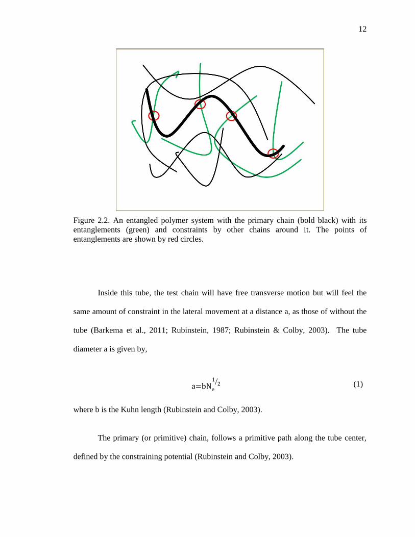
loss of information. A test chain can have many points of entanglements with other chains

around it, but it is assumed that with a single chain, it is entangled at a single point (Mead

et al., 2015). Thus, if there are four entanglements present in a chain, then they are all from

four different chains around it (see Figure 2.2., which depicts an entangled polymer system

with the primary chain and its entanglements). When a system of entangled polymers is

11

under deformation, by virtue of thermodynamics, it tries to arrive at an equilibrium

condition or a steady state condition. This process of reaching equilibrium is called the

relaxation process (Rubinstein & Colby, 2003; Larson, 1999). There are various ways one

can quantify the relaxation mechanism in terms of mathematical models, like Doi and

Edwards’ tube model and its modifications, stochastic modeling, Brownian dynamic

simulation, etc. (Doi & Edwards 1978a, 1978b, 1979, 1986; Mead et al., 1998, 2015; Park

et al., 2012; Xu et al., 2006). The constitutive “toy” model hereby developed and simulated

is a modification of the Doi and Edwards’ tube model, and thus, the discussion is restricted

to the same (Mead et al., 2015).

As discussed above, the entanglements present in and around the test chain pose a

constraint to its lateral movement, and allowing only certain specific conformations and

movements. Qualitatively, one may imagine a “virtual tube” along the contour of the chain

defined by the sum of all the topological constraints active around the chain.

The tube allows some degree of free movement of the test chain along its contour

in the transverse direction (see Figure 2.3.) (McLeish, 2002). The tube has a radius of a,

which is in the order of the end-to-end length of the chain of entanglement is molecular

weight Me, consisting of Ne monomers. This allows only chains with molecular weights

greater than Me to be strongly affected by the topological constraints around them

(McLeish, 2002). As will be discussed later, the number of entanglements on the chain or

the entanglement molecular weight of the system is derived from the plateau modulus of

the component at a given processing temperature.

12

Figure 2.2. An entangled polymer system with the primary chain (bold black) with its

entanglements (green) and constraints by other chains around it. The points of

entanglements are shown by red circles.

Inside this tube, the test chain will have free transverse motion but will feel the

same amount of constraint in the lateral movement at a distance a, as those of without the

tube (Barkema et al., 2011; Rubinstein, 1987; Rubinstein & Colby, 2003). The tube

diameter a is given by,

a=bNe

12⁄ (1)

where b is the Kuhn length (Rubinstein and Colby, 2003).

The primary (or primitive) chain, follows a primitive path along the tube center,

defined by the constraining potential (Rubinstein and Colby, 2003).

13

If the primary chain is assumed to be consist of N Gaussian random walk sub-chains

of effective step length (Kuhn length) b, then the defining tube will also have a Gaussian

random walk of “curvilinear tube length,” “average contour length,” or “the average

primitive path length” 𝐿𝑒𝑞 = [𝑁𝑁𝑒

⁄ ] 𝑎 = 𝑁𝑏2

𝑎⁄ (McLeish, 2002; Rubinstein & Colby,

2003). The tube can thus, be considered to consist of 𝑍 = [𝑁𝑁𝑒

⁄ ] segments, each of length

a (Rubinstein & Colby, 2003). The term 𝑍 also gives the number of entanglements on the

chain.

The average primitive path length is the shortest possible length of the chain

(shorter than the actual contour length of the chain ‘bN’ by a factor of 𝑎𝑏⁄ = √𝑁𝑒 ) at

which the chain can still feel the topological constraints (McLeish, 2002; Rubinstein &

Colby, 2003).

Figure 2.3. A virtual tube (green color) of radius a, created along the contour length of the

primitive chain is the sum of the constraints around it. The purple colored lines depict the

surrounding strands posing as constraints to the primary chain (black).

14

It is an important concept as it defines the time scale and nature of the entanglement

constraint dynamics (McLeish, 2002). For long chain entangled polymers with N>> Ne,

an almost constant modulus, called the plateau modulus (GNo) is observed in a stress

relaxation experiment. The plateau modulus provides the information regarding the

entanglement molecular weight Me, which, in turn, scales the tube segment being created

around the primitive chain.

For entangled polymer melts the plateau modulus is given as follows (Rubinstein

& Colby, 2003):

GNo

= ρRT

Me

(2)

Here, R is the universal gas constant, T is the temperature, and ρ is the density

(Rubinstein & Colby, 2003).

The tube, which is qualitatively a statistical manifestation, can change by two

distinct ways: a) when the chain transversely moves out of the existing tube in order to

move a larger distance and b) when the tube fluctuates with the chain length fluctuations

(Rubinstein,1987; Rubinstein & Colby, 2003). Figure 2.4 shows that as a chain moves out

of the tube, a new tube starts to form, and at the same time, a part of the old tube gets

destroyed. This type movement of the chain is called “reptation motion”. The term

reptation was first used by de Gennes (1971) due to the snake-like Brownian motion of the

chains (McLeish, 2002). The reptative motion of the will decide the longest characteristic

time of the chain movement, called “reptation time / disengagement time / orientation time”

(𝜏𝑑) (Rubinstein, 1987). The reptation time can be defined as “the time the chain takes to

15

diffuse out of the tube of average length Leq” (Rubinstein & Colby, 2003). The reptation

time (𝜏𝑑) is given by (Rubinstein & Colby, 2003):

τd ≈ Leq

2

De≈

ζb2N3

kTNe (3)

Here, De= kTζN⁄ is the curvilinear diffusion coefficient for the chains describing

the motion inside the tube, with ζN as the Rouse friction coefficient, and k as the Boltzmann

constant (Rubinstein & Colby, 2003).

The chain ends have random Brownian motion, which allows them to take any

random path to diffuse in the surrounding melt. Once the chain reptates out of a tube

segment, it is allowed to take a random walk, and a new tube segment gets formed along

the chosen random path. Similarly, as the chain has a choice of random walk, it can even

retract back in the tube, shortening the primitive path (McLeish, 2002). At very small time

(𝑡 ≪ 𝜏𝑒), the random motion of the chain is not hindered by the topological constraints as

the presence of the tube is not yet felt by the chain. At time 𝑡 = 𝜏𝑒, the chain starts feeling

the presence of the tube (i.e., constraints around it) for the first time. This time 𝜏𝑒 is called

the “Rouse time of entanglement strand of length Neb”. This is the smallest possible

characteristic time for a chain confined in a tube. At any time 𝑡 > 𝜏𝑒, the orientation of the

chain is always restricted by the tube confinement until it completely moves out of the tube

(McLeish, 2002; Rubinstein & Colby, 2003). The Rouse time for the entanglement strand

is given by (Rubinstein & Colby, 2003):

16

τe= ζb2Ne

2

kT (4)

Thus, the relation between the reptation time and Rouse time of the entanglement strand is

given by (Rubinstein & Colby, 2003):

τd

τe

= [N

Ne

]3

= Z3 (5)

Vivoy et al. (1991) provides another similar relationship between the reptation and

entanglement segment Rouse time, (which is considered as the basis for entanglement

calculations in the upcoming sections), as,

τd=3τeZ3 (6)

The Rouse time 𝜏𝑅 of the chain (for Rouse motion), which is the longest relaxation time of

the Rouse model, is given by (Rubinstein & Colby, 2003):

τR= τe [N

Ne

]2

= τeZ2 (7)

Here, the Rouse time of a chain is the time taken by a chain to diffuse a distance of the

order of its size. The Rouse time in the later sections is also considered as the stretch

relaxation time. For a chain trapped inside a tube, the ratio of the reptation time to that of

the Rouse time is given as follows (Doi & Edwards, 1986):

τd

τR

= 3Z (8)

17

Figure 2.4. Reptative motion of the chain out of a tube causes simultaneous tube creation

and destruction along the chain contour length.

In practice, the reptation time 𝜏𝑑 is measured experimentally as the reciprocal of

the frequency at which G’ = G’’. The Rouse time of the chain 𝜏𝑅 is calculated from 𝜏𝑑

using equation 8 (Rubinstein & Colby, 2003; Larson, 1999).

The reptation time 𝜏𝑑 and the Rouse time 𝜏𝑅, are the two major characteristic times

considered for the constitutive “toy” models developed in the later sections. It is also

important to note that for a monodisperse system with a single molecular weight

component under study, there is one Rouse time and one reptation time that are widely

separated numerically (i.e., 𝜏𝑑 ≫ 𝜏𝑅), as can be seen from Figure 2.5a. However, in the

case of a polydisperse system, where there is more than one molecular weight component,

there is more than one reptation and Rouse time, and they may overlap. The wider the

molecular weight distribution, the greater the overlap, as can be seen from Figure 2.5b

18

(Mishler & Mead, 2013a). This concept is a crucial factor in modeling a constitutive

equation for polydisperse entangled polymer systems and is discussed in detail later in

Paper III.

Figure 2.5. Characteristic relaxation times. a) Monodisperse entangled polymer system

where the largest Rouse time and the reptation time are widely separated. b) Polydisperse

entangled polymer system where the Rouse times (stretch relaxation time) and the reptation

times (orientation relaxation time) overlap (redrawn from Mishler and Mead (2013a)).

2.3.2. Polymer Relaxation Mechanism. As discussed earlier, the fundamental

objective of the constitutive model is to quantify the steady state or even the transient

rheological behavior of the entangled polymer system. The process of reaching a steady

condition, or equilibrium condition, after a deformation is called relaxation.

An entangled polymer system reaches its relaxation by a combination of a number

of different mechanisms. The few major mechanisms that are included in the original Doi-

Edwards’ tube model are as follows (Doi & Edwards, 1986):

19

1. Reptation of the primary chain within the matrix of constrains.

2. Fluctuations of the primary chain length along the primitive path within the

matrix of constrains.

3. Constraint release due to the motion of the surrounding chains. This causes two

different relaxation scenarios (Mead et al., 1998):

i. Relaxation by tube shortening

ii. Relaxation by tube reorientation

Reptation of the primary chain was discussed in the previous section. The

movement of an entire chain from an old tube to a new tube (both at the same energy state)

completes one single process of relaxation. For high molecular weight monodisperse, linear

polymer chains, reptation is the governing relaxation mechanism under low deformation

conditions. Initially it was assumed that reptation was the only mechanism to describe the

relaxation process. But gradually, due to discrepancies observed between predicted and

experimental values, it was realized that other non-reptative processes need to be accounted

for (Larson, 1999).

In polydisperse systems (a blend of two or more molecular weight components),

there exist combinations of shorter and longer chains. Under any flow conditions, some of

the topological constraints get removed due to shorter chains moving faster than longer

chains, causing an added relaxation for the longer chain components by a mechanism called

“double reptation” (des Cloizeaux, 1988; Tsenoglou, 1991). The idea behind this concept

is that an entanglement or a constraint is lost if either the test chain or the matrix chain

reptates past the entanglement point (Larson, 1999). Details regarding the double reptation

are discussed in Section 4.

20

Primitive path fluctuation can be most conveniently expressed for branched

polymer chains, where one end of the chain is tethered to a polymer branch point. In such

cases, the chain cannot move back and forth and thus cannot reptate (Larson, 1999). Such

chains relax by a primitive path fluctuation mechanism, also called breathing mode (de

Gennes, 1975).

The fluctuations bring the chain ends inside the tube. As a chain end moves inside,

the tube segment is vacated, and the stress on the chain relaxes (see Figure 2.6.). The free

end of the chain must diffuse to the tether point for a complete relaxation, but such a

condition is not entropically favorable (Larson, 1999). Thus, as the chain ends keep on

moving towards the tether point, the fluctuations increases, and the time required for

relaxation increases exponentially (Doi & Kuzuu, 1980). Hence, a chain that relaxes solely

by primitive path fluctuations will have a spectrum of characteristic times.

Figure 2.6. Primitive path fluctuation mechanism (redrawn from Rubinstein & Colby,

2003).

21

The chain segment near the end of the tube will relax fastest with the time required

increasing as we move towards the interior of the chain. For the chains that can reptate

(both chain ends free), the interior part of the chain will relax by reptation, which will be

much faster than by primitive path fluctuations because reptation controls the longest

relaxation time scale for the chain (Larson, 1999). However, the chain ends will relax faster

by fluctuations than by the process of reptation. For very high molecular weight polymers,

these fluctuations are generally very small and confined to a limited portion of the chain,

so they can be neglected (Larson, 1999).

Constraint release is a situation in which some of the topological constraints on the

test chain get removed automatically due to the flow or deformation. This allows the chain

to relax much faster compared to just reptation, as a portion of the chain gets free to relax

(Pearson, 1987; Mead et al., 1998; Larson, 1999). When these constraints get removed by

the convective flow, it is called convective constraint release (Marrucci, 1996; Marrucci &

Ianniruberto, 1996, 1997; Mead et al., 1998), which is discussed in detail in Section 3.

Now, consider a situation where the relaxation is occurring only by constraint

release and there is no reptation or Rouse motion of the chain. Here, a very small time scale

is considered, 𝑡 < 𝜏𝑅, such that only localized Rouse motion and small segment re-

orientation of the test chain are allowed. In such a situation, constraint release can manifest

itself in two forms, and relaxation will either occur as the tube reorients itself, maintaining

the chain length, or as the chain retracts back (tube shortening), keeping the same

orientation as before, or it may even be some combination of the two (see Figure 2.7.)

(Mead et al., 1998).

22

It is also important to understand that both these mechanisms relax the same amount

of stress when constraint release is the only relaxation mechanism. If reptation, chain end

fluctuations, and chain retraction occur along with constraint release, then the above

equivalence will not hold (Mead et al., 1998). In a situation where relaxation is occurring

by reptation, constraint release, and chain retraction, the orientation of the tube will be a

function of both reptation and constraint release. Similarly, stretch in the tube will be

defined by chain retraction, chain end fluctuations, and tube shortening. In such cases, the

stress relaxed by tube shortening or changes in tube length and tube orientation will be

different, and thus the equivalency is lost (Mead et al., 1998).

Constraint release can be completely neglected only in the cases where either the

isolated test chain is surrounded by a matrix chain of much higher molecular weight

compared to the test chain or if the matrix surrounding the test chain is cross-linked

(Larson, 1999).

Many experimental observations (Lodge et al., 1990; Ylitalo et al., 1990; Kremer

& Grest, 1990) have validated the presence of reptation in an entangled polymer system by

the virtue of the fact that the interior of the chain relaxes much slower than the chain ends.

The same experiments also verify that the entire chain relaxation mechanism cannot be

explained by reptation alone. There are other relaxation processes occurring along with

reptation, like constraint release and primitive path fluctuations (Larson, 1999). Further

studies have elucidated that the above mentioned mechanisms are just the most basic of the

processes occurring when an entangled polymer system is deforming.

23

Figure 2.7. Constraint release mechanism. When constraints get removed, the chain can

relax by tube shortening, by tube orientation, or by a combination of the two [redrawn from

Mead et al., 1998].

There are various other physics like tube stretch or incomplete chain retraction,

reduction in friction in the system due to the chain/tube orientation (configuration

dependent friction coefficient), fall in number of equilibrium entanglements with

deformation (entanglement dynamics), and others which need to be considered while

developing the constitutive equations so as to provide accurate qualitative and quantitative

descriptions of the rheological behavior (Marrucci & Grizzuti, 1988; Marrucci, 1996; Mead

et al., 1998, 2015; Park et al., 2012). These topics are subsequently discussed in the later

sections and Papers II and III.

24

3. HISTORY OF MONODISPERSE SYSTEM CONSTITUTIVE “TOY” MODEL

DEVELOPMENT

The constitutive models used to study the rheological behavior of linear entangled

monodisperse polymers under low and high flow conditions have evolved over time. As

discussed in the previous section, de Gennes proposed the concept of reptation, which was

further developed by Doi and Edwards to introduce tube theory. This theory provides the

ground work for the subsequent models that have been developed in the last five of decades.

Though most of the models are in excellent agreement with the linear rheological behavior

of the linear entangled melts and solution, they start to differ in their nonlinear behavior

predictions under high flow conditions. Nonlinear flow conditions are still not well

understood and have been under investigation since last forty years.

Doi-Edwards (DE) tube model works well for all low flow deformation conditions

where the behavior is predominantly linear. It is based on two major relaxation mechanisms

of reptation and complete chain retraction within the constrain matrix, under affine

deformation (Doi & Edwards, 1978a, 1978b, 1979, 1986). The model is also based on the

assumption of a constant number of equilibrium entanglements on the chain under any

flow. It also assumes that the constraints are fixed. Though the model very accurately

predicts the nonlinear deformation of the linear entangled monodisperse polymer melts

under step-shear strains, it fails to both qualitatively and quantitatively predict the nonlinear

behavior under other forms of deformations like steady shear and extension (Mead et al.,

1998). One major drawback of the theory is the mechanism of “complete chain retraction.”

Under fast flow conditions, the chain starts stretching, which means that the length

occupied by the tube increases above that of the equilibrium length (Doi & Edwards,

25

1978a, 1978b, 1979, 1986). Simultaneously, the chain is also allowed to retract back in the

tube (i.e. the chain moves back along the contour of the tube). According to Doi-Edwards

proposition, the chain retraction time (Rouse relaxation time 𝜏𝑅) is faster than the strain

rates or the reptation time 𝜏𝑑. Consequently, the chain completely retracts back in the tube

after getting stretched and thus maintains a constant equilibrium tube length in any flow

(Doi & Edwards, 1978a, 1978b, 1979, 1986; Mead et al., 1998; Larson, 1999). This

resulted in the over-prediction of the steady shear thinning behavior for the linear polymer

melts and a failure to quantitatively predict the overshoots observed in the transient first

normal stress difference curve.

The next improvement in the model, called the Doi-Edward-Marrucci-Grizzuti

(DEMG) model, was brought about by Marrucci and Grizzuti in 1988. They modified the

chain retraction concept (keeping the assumptions of a constant number of equilibrium

entanglements and fixed constraints), and initiated that the retraction process is gradual and

incomplete. This implies that there is a finite amount of chain stretching observed above

the equilibrium chain length (Marrucci & Grizzuti, 1988; Mead et al., 1998). This concept

should have improved the results compared to the DE model, as chain stretching should

have increased the predicted shear viscosity. But the entire physics of the model was such

that under high shear flow, the tubes got highly oriented in the direction of the flow, causing

a loss in the drag. This caused a collapse in the tube stretch effect, lowering the viscosity

and reducing the results to same as that of the DE model prediction (see Figure 3.1.)

(Larson, 1999; Mead et al., 1998, 2015).

Nevertheless, the tube stretching did improve the overshoot predictions for the first

normal stress difference and shear stress. The model also failed to predict the monotonic

26

extension thinning behavior observed for melts (see Figure 3.2.) (Mead et al., 2015). Both

DEMG and DE also predicted that with increase in molecular weight, the melt shear

viscosity decreases with increase in high shear rate, under shear thinning regime; which is

contrary to the fact that at high shear rates, the shear viscosity is a very weak function of

molecular weight (Mead et al., 1998). Thus, even though the physics behind the theory was

improved, the DEMG model still could not improve the predictions for steady shear and

steady extensional viscosities over that of the DE model. The simplest constitutive

equations for the above concept were presented by Pearson et al. (1991).

In 1996 Marrucci, Ianniruberto and Marrucci (1996), introduced another concept

called convective constraint release (CCR). Under slow flow, constraint release may not

be of much consequence, but under fast flow conditions (at strain rates greater than 1𝜏𝑑

⁄ )

by the virtue of the flow itself, some of the topological constraints around the primary chain

get removed automatically. In this case, the assumption of fixed tube no longer holds true.

This allows the chain to relax much faster compared to relaxing just by reptation. The

simplified models developed by Ianniruberto and Marrucci (1996), using the concept of

CCR, are based on an assumption that all parts of the molecule experience the same

orientation and degree of stretch. One important fact that needs to be elucidated is that not

all types of convections can release constraints. If the system is affinely deformed in such

a way that all the chains have the same deformation, then both the primary chain and the

surrounding matrix chains will deform together. Hence, there will be no constrain release

(Ianniruberto & Marrucci, 1996; Marrucci & Ianniruberto, 1997). Thus, the convective

constraint release occurs only when the matrix chains around the primary chain are

undergoing retraction. As the length of matrix chains reduces, the constraints on the

27

primary chain get removed. New constraints replace the old ones, but during the process

of replacement, the primary chain relaxes (Ianniruberto & Marrucci, 1996; Larson et al.,

1998; Mead et al., 1998). To account for the relaxation by constraint release, Ianniruberto

and Marrucci (1996) considered time-dependent tube diameter. The reduction in bond

orientation order caused by constraint release is accounted for by increasing the tube

diameter and thus reducing the length of the primitive path of the tube (Ianniruberto &

Marrucci, 1996; Marrucci & Ianniruberto, 1997).

Mead, Larson, and Doi (1998) developed the MLD “toy” model, which is an

improvement of the DEMG model, and incorporated the mechanism of CCR into it. The

MLD model also allows relaxation of chain ends to occur by fluctuations and improved on

the concept that both the chain orientation and degree of stretch are functions of tube

coordinates (based on contour variable theory), thus removing the assumptions made by

Ianniruberto and Marrucci (1996) in the previous CCR models. The MLD “toy” model like

its predecessors, is based the concept of a constant number of equilibrium entanglements,

as any entanglement dissolved is immediately replaced by a new one (Mead et al., 1998).

Depending on the tube stretch conditions, the CCR effect will manifest itself in either tube

orientation or tube shortening.

If the chain is stretched beyond the equilibrium condition (λ > 1), then it is unable

to explore the entire volume of the tube, and constraint release will cause tube shortening.

On the other hand, for chains not under tension (λ = 1), the chain will be slack enough to

explore the tube volume and thus allow it to escape the tube, leading to tube reorientation

(Mead et al., 1998).

28

Figure 3.1. Steady shear viscosity vs shear rate curve showing DEMG, MLD, and

experimental results for 200KPS monodisperse melt. DEMG over-predicts the shear

thinning behavior, where the MLD model has an improved prediction due to the effect of

CCR incorporated in it (Mead et al., 2015).

The MLD “toy” model definitely improved the predictions for the steady shear

viscosity for linear monodisperse entangled melt, as can be seen from Figure 3.1.,

confirming that CCR is an important physics to describe the shear system at high

deformation condition. The effect of CCR is prominent before the tube starts stretching.

Contrariwise, as can be seen from Figure 3.2., the MLD “toy” model, similar to DEMG

model, could not predict the extension thinning behavior of the monodisperse melt (Mead

et al., 2015). From this one may conclude that CCR effect may not be the physics to define

the extension thinning observed at high deformation rates.

29

Figure 3.2. Steady extensional viscosity vs extension rate curve showing DEMG, MLD,

and experimental results for 200KPS monodisperse melt. Both DEMG and MLD predict

an extension thickening behavior under high extension conditions, where experiments

show an extension thinning behavior (Mead et al., 2015).

Though the steady shear behavior has been explained using the MLD model by

incorporating CCR, the steady extension melt thinning related issues have not yet been

dealt with. In 2012, two independent research groups working on two completely different

approaches to tackle the extensional entanglement polymer rheology issues (Park and

group using stochastic simulation and Yaoita et al. using the tube theory way (Park et al.,

2012; Yaoita et al., 2012)), proposed similar concept called the configuration dependent

friction coefficient (CDFC).

30

The idea of CDFC was initially developed by Ianniruberto et al. when it was

proposed that when the stretch and orientation of the chain occurs, there will be a loss of

monomeric friction ζ (Ianniruberto et al., 2012). MD simulations and recent experimental

studies have also validated the presence of reduction in the friction factor when the polymer

system is highly stretched and oriented (Andreev et al., 2013; Wingstrand et al., 2015).

Yaoita et al. then validated that the friction coefficient as a function of stretch/orientation

factor 𝜁(𝐹𝑆𝑂) remains at equilibrium when (𝐹𝑆𝑂) is increased to a certain threshold value

(≈ 0.15), after which it starts steeply decreasing with a further increase in the

stretch/orientation factor. Here (𝐹𝑆𝑂) = 𝜆2𝑆 , where �� = 𝜆

𝜆𝑚𝑎𝑥 and 𝑆 are the averaged

anisotropic orientation of all components (Yaoita et al., 2012, 2014).

When incorporated in the constitutive MLD equation, they showed that a reduction

in the friction coefficient can very much be the reason for the observed steady extension

thinning behavior in linear polymer melts when the system is highly stretched and

orientated (Yaoita et al., 2014). In their stochastic simulation, Park et al. also verified that

CDFC is definitely the key to the extension thinning behavior of the linear polymer melts

at high extension rates (Park et al., 2012). Further discussion on CDFC and how the concept

is incorporated in describing the constitutive equations is taken up in Paper II.

The new constitutive “toy” model called the Mead-Banerjee-Park (MBP)

monodisperse model and developed by the authors, is a modification of the MLD “toy”

with the incorporation of two major concepts: a) CDFC and b) entanglement dynamics

(ED). Until now, all the major modified tube models that have been developed were based

on the assumption of a constant number of entanglements, irrespective of the flow.

31

The models assumed that with CCR when the entanglements get destroyed new

entanglements take its place and thus the total number of equilibrium entanglements remain

fixed. But under fast deformation when the strands are unraveling, orienting and getting

stretched, the number of entanglements on the chain cannot remain fixed. The same

phenomenon was also observed by Baig et al. (2009) in their Brownian dynamic simulation

of entangled linear polymers. Thus the above assumption was modified in the new model

to define an idea of entanglement dynamics where the number of equilibrium

entanglements on the chain alters with deformation (Mead et al., 2015). Details regarding

the model development, simulations, and results are presented in Paper II.

32

4. HISTORY OF POLYDISPERSE SYSTEM CONSTITUTIVE “TOY” MODEL

DEVELOPMENT

Similar to the model development discussed for the monodisperse systems the

polydisperse constitutive “toy” model development also starts with Doi and Edwards’ tube

model as the base. The DE model failed to describe the polydisperse conditions because of

its assumption that the constraint matrix around the test chain is fixed (single reptation of

only the test chain). This implies that the movement either by reptation or chain retraction

occurs only in the primary chain (Doi & Edwards, 1986). As pointed out earlier, in a

polydisperse system, more than one molecular weight component is blended together;

consequently, there will be complex entanglements of shorter and longer chains. Each of

these chains will have its own reptation and Rouse time of motion, and thus, the

entanglements will also have different lifetimes. The entanglements of long-short chains

will dissolve much faster than long-long entanglements as the short chain moves faster than

the long chains. Thus, this will allow the long chains to relax faster by constraint release

(Larson, 1999; Auhl et al., 2009; Mishler & Mead, 2013a, 2013b). In such a scenario it is

erroneous to assume that the matrix chain that creates the constraint around the test chain

is constant.

A semi-empirical concept of “double reptation” was proposed and implemented by

multiple researchers to overcome the incongruity of Doi and Edwards’ model (Rubinstein

& Colby, 1988; Tsenoglou, 1987, 1991; des Cloizeaux, 1988, 1990). Applications of

monodisperse models to polydisperse systems have always proven to be difficult, due to

their inherent complexities, and the double reptation model has proven to be one of the

most successful models to describe polydispersity in recent times.

33

The idea in a simplistic approach can be thought of as a combination of reptation

and constraint release. According to this proposed theory, the test chain and the

surrounding chains are allowed to reptate together. The proposed theory provides accurate

predictions of G’ and G’’ for a specified molecular weight distribution, for both bidisperse

and polydisperse systems (Wasserman & Graessley, 1992). Another positive feature of this

model is that it has no added parameters over the original DE model (single reptation). The

inversion of the double reptation mixing rule could also be used to generate the molecular

weight distribution of the system, analytically and numerically, from its rheological

behavior as described by Mead (1994).

The MLD “toy” model for monodisperse systems was modified based on binary

interaction theory and generalized double reptation with a slip-link entanglement survival

probability equation to account for polydispersity (Mead et al., 1998; Mead, 2007).

Although the model could successfully predict some of the polydisperse rheology behavior,

the physics behind the system was not sound. It was mostly based on the idea that the basic

underlying physics in monodisperse and polydisperse systems are same and thus can be

easily generalized without adding any new mechanism. The complexities behind the

entanglements present and their probable effects on the entire system were not considered

important (Mishler & Mead, 2013a).

In 2009, Auhl et al. made an effort to explain the behavior of bidisperse

polyisoprene (PI) systems under uniaxial extension using a concept of nested tube (Auhl

et al., 2009). The major motivation behind the theory is the fact that in polydisperse system,

multiple constrain release rates exist and that the elongation hardening that is observed

(deviation from linear viscoelastic behavior) is related to the long chain component’s

34

stretch relaxation. Consider a bi-blend (same material) system of widely separated

molecular weights mixed together such that there are two types of chains in the blend: long

chains and short chains. This implies that there are four major types of entanglements

present in the system: a) long-long, b) long-short, c) short-long and d) short-short. Thus,

for the long chains, the two types of entanglements will have two different constraint

release rates, and the long-short will dissolve faster than long-long.

Thus, one can imagine (see Figure 4.1.), two tubes around the long chains with the

thin tube defined by all the entanglements and the thick tube given by only the long-long

entanglements. The presence of the short chain component is considered to create a dilution

effect, and thus their entanglement effects are not considered. The long chain component

and the effect of short chain dilution on the stretch relaxation are analyzed and are believed

to be responsible for the stress generated in the system. The presence of short chains and

the stress related to them are neglected as they are considered to provide the dilution effect

only (Auhl et al., 2009).

Figure 4.1. Nested tube model proposed by Auhl et al. (2009). The primary tube is defined

by all the entanglements whereas the diluted tube is given by only the long entanglements

35

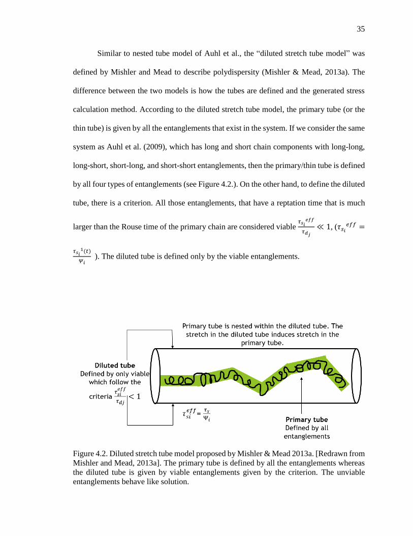
Similar to nested tube model of Auhl et al., the “diluted stretch tube model” was

defined by Mishler and Mead to describe polydispersity (Mishler & Mead, 2013a). The

difference between the two models is how the tubes are defined and the generated stress

calculation method. According to the diluted stretch tube model, the primary tube (or the

thin tube) is given by all the entanglements that exist in the system. If we consider the same

system as Auhl et al. (2009), which has long and short chain components with long-long,

long-short, short-long, and short-short entanglements, then the primary/thin tube is defined

by all four types of entanglements (see Figure 4.2.). On the other hand, to define the diluted

tube, there is a criterion. All those entanglements, that have a reptation time that is much

larger than the Rouse time of the primary chain are considered viable 𝜏𝑠𝑖

𝑒𝑓𝑓

𝜏𝑑𝑗

≪ 1, (𝜏𝑠𝑖

𝑒𝑓𝑓 =

𝜏𝑠𝑖1(𝑡)

𝛹𝑖 ). The diluted tube is defined only by the viable entanglements.

Figure 4.2. Diluted stretch tube model proposed by Mishler & Mead 2013a. [Redrawn from

Mishler and Mead, 2013a]. The primary tube is defined by all the entanglements whereas

the diluted tube is given by viable entanglements given by the criterion. The unviable

entanglements behave like solution.

36

Those entanglements that have an average lifetime less than the effective Rouse

time of the test chain 𝜏𝑠𝑖

𝑒𝑓𝑓

𝜏𝑑𝑗

> 1, (𝜏𝑠𝑖

𝑒𝑓𝑓 =𝜏𝑠𝑖

1(𝑡)

𝛹𝑖 ) act as a solvent with respect to the

stretch relaxation process. The major factor behind the criteria is that the chains have

different lifetimes, and there are constraints that move away much faster than the primary

chain Rouse motion, thus not effecting the stretch dynamics of the primary chain. The

stretch generated in the diluted tube is coupled with that of the primary tube, and the stress

is given by all the entanglements that are present in the system, and not only by the ones

that define the diluted tube (Mishler & Mead, 2013a, 2013b).

The MBP polydisperse model is based on the concept of “diluted stretch tube”

theory incorporated in the MBP monodisperse model. Thus the MBP “toy” model for the

polydisperse system will have the same physics of CCR, ED and CDFC as that of the

monodisperse condition along with stretch tube dilution. The details regarding the

constitutive model development, simulation, and results are discussed in Paper III.

37

PAPER

I. Modeling and simulation of biopolymer networks: Classification of the

cytoskeleton models according to multiple scales

Abstract

We reviewed numerical/analytical models for describing rheological properties and

mechanical behaviors of biopolymer networks with a focus on the cytoskeleton, a major

component of a living cell. The cytoskeleton models are classified into three categories:

the cell-scale continuum-based model, the structure-based model, and the polymer-based

model, according to the length scales of the phenomena of interest. The criteria for

classification of the models are modified and extended from those used by Mofrad [M. R.

K. Mofrad, Annual Rev. Fluid Mech. 41, 433 (2009)]. The main principles and

characteristics of each model are summarized and discussed by comparison with each

other. Since the stress-deformation relation of cytoskeleton is dependent on the length scale

of stress elements determines, our model classification helps systematic understanding of

biopolymer network modeling.

38

INTRODUCTION

Recent studies in the field of medicine have elucidated the need to understand how

the structures of biopolymers and the various physical forces acting on them contribute to

the synthesis, growth, transportation, information processing and functioning of living cells

and tissues. Many of these forces and their effects have been identified and studied, such

as hemodynamic shear stress on vascular tissues, inspiratory pressure on lung functions,

tension on skin ageing etc. [1]. In addition, numerous diseases, including tumours, lung

cancer, emphysema, neuro-degeneration, pulmonary fibrosis, etc. [2-4], have been

associated with the change of these physical forces and, subsequently, the biopolymer

structures. These physical forces have also been found to be vital for cellular and genetic

regulation in the living body [5].

Living cells dynamically respond to any mechanical perturbations in their

environment solely by altering the cytoskeleton configuration and functioning [6, 7]. The

cytoskeleton is a network of protein tubules present inside a cell, and is responsible for

cellular structure, shape, movement and growth. Cells are adhered to a scaffold called the

extra-cellular matrix. During the process of cell growth and movement, the cellular forces

in the scaffold and inside the cell are balanced by the cytoskeleton [8-11]. Even the

interactions between two adjacent cells are affected by the mechanical behavior of the

cytoskeleton [12]. Thus it is imperative to identify the various mechanical forces and

analyze their effects on the structure and behaviors of the cytoskeleton in order to

understand cell functioning and abnormalities. This knowledge will lead to a better

understanding of the causes of disease and corresponding cures.

39

There have been numerous efforts to model the relationships between the structure

of the cytoskeleton and its rheological properties and mechanical behaviors. However, due

to the cytoskeleton’s complex structure and heterogeneous components, no single approach

has been able to accurately encompass all of its various behaviors. As shown in Figure 1,

the cytoskeleton network is composed of three main highly entangled protein structures:

actin filaments, microtubules and intermediate filaments. These components together are

responsible for the properties and mechanics of the cells [13].

The actin filament (or F-actin), a filamentous form of monomeric G-actin protein,

is the major component of the cytoskeleton, comprising up to 10% of the total cellular

protein mass [14]. It has a persistent length about 15 – 17 µm [15]. The F-actin further

cross-links to create a bundle or an orthogonal cytoskeleton network structure by the cross-

linking of actin binding proteins [15-21]. The F-actin filaments are also continuously

undergoing polymerization and depolymerization, leading to an active network structure

[15, 22-24]. These cross-linkers and the degree of crosslinking also lead to strain stiffening

behavior exhibited by the F-actin [13, 25].

Microtubules, the second major component of the cytoskeleton network, exhibit

hollow cylindrical shapes composed of monomers α and β – tubulin with persistent lengths

of 6 mm [13,15]. They have higher bending stiffness, are more active in nature than actin

filaments, and continuously undergo polymerization and depolymerisation [25, 26]. The

microtubules are known to be the compressive load-bearing component of the network as

balanced against the tensed actin and intermediate filaments [27].

40

The intermediate filaments (persistence length ~ 1 m) are the least well studied of

the three components of cytoskeleton [13,15]. They, along with F-actin, act as the tension-

bearing components under deformation and have a rope-like structure consisting of

different proteins [12-13, 25]. They are more stable compared to F-actin and microtubules

and can withstand higher stresses and strains before rupture [25].

The dynamics and properties of the cytoskeleton result from the collective actions

of the aforementioned components at various time and length scales. Therefore, successful

modeling of the cytoskeleton requires proper approximation of the behaviors and properties

of those structural elements for the time and length scales of the phenomena of interest.

The length scale is important for thermal and mechanical effects. However, biological

effects or structural reorganization (including polymerization/depolymerization) must

consider both length and time scales. For example, the stress-deformation behaviors within

a time scale range where there is no structural reorganization or

polymerization/depolymerization are referred as “passive dynamics,” whereas “active

dynamics” are related to biological responses at longer time scales [13].

This review paper classifies numerous analytical and numerical models used to

analyze cytoskeleton behaviors and properties into three groups according to length scales:

cell-scale continuum-based models, structure-based models, and polymer-based models,

as shown in Figure 1. We focus on models used to analyze the passive dynamics of the

cytoskeleton. Length scales of individual cell mechanical properties range from atomistic

to the macroscopic cell level. It is also noteworthy that we exclude models that work at the

scale of collective cell motions (> 10 m).

41

Our classification is adapted from that used by Mofrad’s review in 2009 [13].

Models, which describe the dynamic behaviors of a single cell as an elastic continuum

medium, are classified as “cell-scale continuum-based models”. Mofrad named similar

models “continuum-based models”, but we add “cell-scale” (typically around 10 m [28])

to distinguish them from continuum approaches at smaller scales [28]. “Structure-based

models” elucidate cytoskeleton properties with discrete representative volume elements

(RVE) which approximate the stress-deformation relationship among structural

components (typically between 1 and 10 m [28]). As this model name was used in Chen’s

review in 2014 [29], these models encompass the groups of “tensegrity models” as

classified in Mofrad [13], the models reviewed by Chen and co-workers in 2012 [30], and

the continuum polymer network models summarized in a review by Unterberger and

Holzapfel in 2014 [28]. The “polymer-based model” explains the cytoskeleton properties

in terms of polymer network structures (typically around 1 m [28]) or a single polymer

molecule (less than 10 nm [28]), as in Mofrad [13].

Many reviews have summarized various models for cellular and cytoskeleton

dynamics using different approaches. As mentioned, Mofrad provided a unified insight into

the overall cytoskeleton rheology and experimental techniques [13]. However, additional

structure-based and polymer-based models have subsequently been added to other reviews.

Chen and co-workers summarized models by focusing particularly on the structure-based

models [30]. Chen’s review classified models into continuum-based and structure-based

models. However, the author specifically arranged continuum-based models related to

indentation experiments into another separate group: nanoindentation models. [29]. Nava

and co-workers [31] and Moeendarbary and Harris [32] have unified various models

42

ranging from cell mechanics (>10 m) to cytoskeleton behaviors (~1 m). The former,

which is mostly related to mechanics of adherent cells, proposed a model classification that

included only continuum-based models and structure-based models (they used terms of

continuum model and microstructural model). The latter models depict various cell

phenomena at different time scales and length scales (but do not provide much detail on

cytoskeletons). There were other reviews [28, 33, 34] which mainly emphasized polymer-

based models (from molecular level to network scale), but did not provide much discussion

of cell-scale and structure-based models.

Our aim is to provide a systematic understanding of cytoskeleton models in terms

of length scales, which determine the stress-deformation relation of the cytoskeleton. This

paper summarizes the underlying principle, main application, and advantages and

disadvantages of cytoskeleton models in each classified length scale group.

43

CELL-SCALE CONTINUUM-BASED MODELS (~10 M)

The cell-scale continuum-based models describe the mechanical/rheological

behaviors and properties of a cell at cellular length scales (typically ~10 m), which is

larger than the typical distance between different cell components [28]), by assuming that

cell cytoplasm is a homogeneous and continuous medium. These models are usually used

for the simulation of cell motions (migration, spreading, etc.) or experiments for cell

property measurements [35]. Based on the level of simplification and the behaviors of

interest, these models can be further classified into elastic/viscoelastic models, multi-

phasic models and soft glassy models.

1. Elastic/Viscoelastic Models

Elastic/viscoelastic continuum-based models utilize Cauchy’s momentum equation

as well as constitutive equations that represent the stress-strain behavior of the cytoskeleton

as a homogeneous elastic or viscoelastic medium [13]. A cell cytoplasm is discretized into

small computational units (mesh) to solve those model equations by the finite element

method with necessary boundary conditions. The major application of this approach is for

analysing and evaluating the cells’ experimentally measured in vivo and in vitro force

levels and their effects on cell behaviors [36]. It gives adequate results when measuring the

cell deformation macroscopically [37, 38].

These models are classified into elastic models or viscoelastic models depending

on the dynamic time scale of the cellular behavior of interest [13]. An elastic model is

sufficient to describe small deformations following Hook’s law, whereas a nonlinear elastic

44

model, such as the Gaussian model, is required for larger deformations [29]. However, the

elastic models are only suitable for modeling cell material properties and cell dynamic

behaviors at limited time scales (near equilibrium) due to their oversimplification [29, 31].

The time-dependent stress-strain behaviors can be described by the viscoelastic

models that utilize typical viscoelastic constitutive equations, such as typical or modified

Maxwell model [31, 32]. Viscoelastic models have been able to predict the cellular

mechanics for blood cells, which are under continuous shear and high mechanical

perturbations, as well as for adherent cells such as epithelial and endothelial cells [39].

Recently, a 2D viscoelastic model was used to simulate cell migration in a microchannel

[39]. A recent 3D constitutive model was extended to simulate lipid bilayer-cytoskeleton

coupling in an erythrocyte membrane [40].

2. Multiphasic Model

The multiphasic continuum model was first proposed by Guilak and co-workers,

based on the idea that the viscoelastic behaviors of cells can be attributed to the intrinsic

viscoelastic property of the cytoskeleton (solid phase in cytoplasm), the fluid viscosity of

the interstitial fluid (cytosol: water with ions), and the solid-fluid interaction within a cell

[41]. The basic approach of the biphasic cell model [42] can be extended to a more realistic

physical representation of a cell by adding more phases. Therefore, the biphasic approach

requires constitutive stress-strain equations in each phase as well as additional momentum

and mass conservation equations over those phases. For example, the triphasic model

considers a viscous liquid phase, an elastic solid phase, and an ionic phase, where two

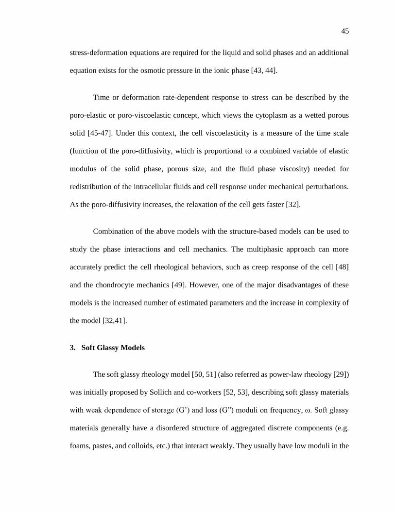
45

stress-deformation equations are required for the liquid and solid phases and an additional

equation exists for the osmotic pressure in the ionic phase [43, 44].

Time or deformation rate-dependent response to stress can be described by the

poro-elastic or poro-viscoelastic concept, which views the cytoplasm as a wetted porous

solid [45-47]. Under this context, the cell viscoelasticity is a measure of the time scale

(function of the poro-diffusivity, which is proportional to a combined variable of elastic

modulus of the solid phase, porous size, and the fluid phase viscosity) needed for

redistribution of the intracellular fluids and cell response under mechanical perturbations.

As the poro-diffusivity increases, the relaxation of the cell gets faster [32].

Combination of the above models with the structure-based models can be used to

study the phase interactions and cell mechanics. The multiphasic approach can more

accurately predict the cell rheological behaviors, such as creep response of the cell [48]

and the chondrocyte mechanics [49]. However, one of the major disadvantages of these

models is the increased number of estimated parameters and the increase in complexity of

the model [32,41].

3. Soft Glassy Models

The soft glassy rheology model [50, 51] (also referred as power-law rheology [29])

was initially proposed by Sollich and co-workers [52, 53], describing soft glassy materials

with weak dependence of storage (G’) and loss (G”) moduli on frequency, ω. Soft glassy

materials generally have a disordered structure of aggregated discrete components (e.g.

foams, pastes, and colloids, etc.) that interact weakly. They usually have low moduli in the

46

range of Pa to kPa, and are not thermodynamically stable. Based on the above observations

of the resemblance of the cytoskeleton to soft glassy materials, the soft glassy rheology

was proposed as another interpretation of the continuum-based cytoskeleton model to

elucidate how the macroscopic cellular response is related to the localized structural

rearrangements caused by meta-stability and disordered structure [32, 50, 51]. This model

can adequately predict the frequency dependency of elastic and loss moduli for all animal

tissue types, including the smooth muscles in human airway, endothelial and epithelial

cells, for a wide time range of ~0.001 – 100 sec using a universal parameter called a noise

temperature. However, microscopic interpretation of this parameter has not been

performed [50].

4. Discussion of the Cell-scale Continuum-based Models

The aforementioned cell-scale continuum-based models have been widely used for

simulation of whole cell behaviors as well as for cell material property experiments.

According to the conditions of the behaviors of interest, different models can be chosen.

For example, even for simulation of the same micropipette aspiration experiments,

different models have been chosen according to the ranges of deformation and time

[48,54,55].

There are some major disadvantages with all of the above continuum-based models.

Firstly, these models emphasize macroscopic cellular behaviors and dynamics.

Microstructure and individual cytoskeleton component behaviors are not considered by

approximation at the continuum level. For example, the effects of actin cross-linkers,

thermal fluctuations, and polymerization/depolymerization are neglected. Therefore, the

47

interpretation of the molecular level interactions is not allowed. Additionally, the

macroscopic models cannot predict and understand the pre-stressed phenomenon observed

in the cytoskeleton network [56]. The structure-based models and the polymer-based

models, which will be discussed in the subsequent sections, portray a better understanding

of cytoskeleton properties and behaviors from a microstructural point of view.

48

STRUCTURE-BASED MODEL (1~10 M)

Structure-based models utilize discrete structural elements, which represent the

individual stress-strain relationships among the microstructural components of the

cytoskeleton, to describe the rheological properties and mechanical behaviors of the

cytoskeleton [29, 32]. Since the heterogeneity of the cytoskeleton is considered through

the microstructural stress elements, these models can describe some cell behaviors that

cannot be simulated by the cell-scale continuum-based models, such as stability of the cell

shape and cell stiffness [56]. The structure-based models can be further categorized into

two groups: the pre-stress (pre-existing tensile stress) models and the semi-flexibility

models. Pre-stress models, which include the cortical membrane model, the tensed cable

nets model, and the tensegrity (cable and strut) models, consider pre-stress in the

intercellular force balance to predict cell shape [56]. Note here that some reviews, such as

by Mofrad [13], named all pre-stress models as tensegrity models. Semi-flexibility models

include open cell foam models, the semi-flexible network element model (‘element’ is

added to be distinguished from other polymer-based network models), and continuum

polymer network models, which utilize RVE to the represent coarse-grained semi-flexible

actin network [30]. The pre-stress model is important because it is known that the pre-stress

is related to the cell shape stability and the cell stiffness [56]. The semi-flexibility model

relates the bending ability of actin filaments with cell behaviors, such as strain hardening

[30, 31]. Since the stress elements of these models consider the cytoskeleton components,

the element length scales are considered to be smaller than cell scale (<10 m) [28].

However, since the stress element is still an imaginary representation of the actual polymer

network, the element length scale is considered to be larger than the polymer network scale

49

(>1 m) [31, 56]. These models consider affine approximation (local deformation is the

same as the macroscopic deformation) of the discrete elements, allowing continuum

interpretations of the deformations, resulting in less numerical and computational

complexity than the polymer-based models [56].

1. Cortical Membrane Model

This model assumes that the stress bearing elements of the cytoskeleton are

restricted within a thin or several thin distinctive cortical layers with the stress balanced

either completely by the pressurized cytoplasm itself, or by the cytoplasm and extracellular

matrix together [57]. This model can also predict the linear stress and cell stiffness

relationship and give a good approximation for suspended cell (e.g. blood cells) and non-

adherent cell behavior [58, 59]. The major disadvantage of this model is that its primary

assumption, that the resistance to cell shape alteration is provided by a thin cortical layer,

cannot be applied to adherent cells [60]. Thus, the limitation of this model inspired the

shell-like 3D pre-stress models in the next section [30, 56].

2. Tensed Cable Nets Models

This concept models a network completely constituted of tensile cable elements

(linear-elastic springs) without the balanced compression in the microtubules. The pre-

stress is maintained and supported by the external extracellular matrix. The model predicts

a linear relationship between stiffness and stress when the cable tension is constant;

otherwise, the trend is non-linear [56]. As in the cortical membrane model, the pre-stress

in the cortical membrane can be simulated with 2D tensed cable nets [59, 61, 62]. One

50

example of a typical 2D cable net (reinforced squared net) is shown in Figure 2. In the case

of the behavior of suspended cells, such as blood cells, this model provides very good

agreement with the experimental observations; however, the behaviors of adherent cells,

such as cell spreading and cell migration, require more complicated 3D models for better

simulation [30, 56].

The 3D tensed cable nets models construct 3D cable networks with uncrossed free-

sliding joints as well as pin joints [63, 64]. The pre-stress is equal to the sum of all the

tensile forces in the cables across a cross-sectional area [63, 65]. This model is also able

to predict some of the mechanical properties, such as Young’s modulus, of the cytoskeleton

and has good accordance with micropipette aspiration experiments. It also provides better

interpretations of cell mechanics compared to the open cell foam models, which will be

introduced later. [30]. Major disadvantages with the model are that they do not include

anything about compressed microtubules and still have limited ability to predict the

behavior for adherent cells [27, 31, 56].

3. Tensegrity (Cable-strut) Models

The tensional integrity, or tensegrity, model employs a discrete network of self-

stabilizing pre-stressed tension bearing components (actin and intermediate tubules) which

are balanced by locally compressed units (microtubules), each subjected to mechanical

equilibrium and geometric deformation [10, 27, 66]. In vivo probing has elucidated that the

actin filaments are the stiffest of all cytoskeleton components with a linear shape, whereas

the microtubules appear curved. Thus, the principal assumption of this model is that actin

and intermediate tubules are the stress bearing components but the microtubules resist

51

compression, which is in accordance with the above observations [10, 67, 68]. The stress

element of this model is based on variations of R. Buckminster Fuller’s tensional integrity

structure, proposed in 1961 [69]. This model describes a network system stabilized by

continuous tension rather than continuous compression units [27]. Thus, the mechanical

stability of the network depends on the arrangements and re-arrangements of these

components. One of the most typical tensegrity elements, the octahedral structure, is shown

in Figure 3. This basic structure consists of six rigid struts (compression-resisting elements)

and 24 elastic cables (tensile-bearing elements). Depending on the experimental conditions,

more complicated structures [70], viscoelastic cables [71], additional tensegrity elements

and cables for nucleus and intermediate filaments [10, 72], and multimodal or additional

tensegrity elements [10, 73, 74] can be added.

The model correctly predicts the linear increase in stiffness of the network with that

of the applied stress in accordance with experimental results [27, 56]. This model can also

predict both static and dynamic behavior of various cell types (e.g., human airway smooth

muscle cells and the adherent cells) and has confirmed that the cells maintain their shape

by redistributing and balancing the stress between the cytoskeleton and the extracellular

matrix [31, 32, 56]. The pre-stress and subsequent increase in cell stiffness as predicted by

this model can probably also explains the high elasticity and non-linear viscoelastic

behaviors observed in cells [32]. In contrast, this model still has the disadvantage in the

prediction of the elastic modulus greater than experimentally measured values and the

limitation in the description of cell viscoelastic behaviors, which requires consideration of

polymer structure at smaller scales [28, 30].

52

4. Open Cell Foam Model

In this model, the actin network is a rigid cross-linking of beam-like structures, of

which shape is either cuboid, dodecahedron, tetrakaidecahedron, or icosahedron, with

bending and twisting of the struts as the major stress-generating component. One of the

typical stress units is a cuboid as shown in Figure 4a. [30, 75]. This model has a major

application when studying endothelial cells. It can also predict the strain hardening under

compression for the adherent cells exposed to local mechanical perturbations [31]. The

open cell foam model does not include pre-stress and thus does not elucidate the effect of

stress on cell stiffness. The rigidity of the cross-link is a major disadvantage of the model,

as in reality the actin cross-links are not rigid [12]. Overall, this model may not be able to

provide as much information regarding cytoskeleton mechanics compared to the other

models [30, 31].

5. Semi-flexible Network Element Model

We named this model as “semi-flexible network element model” because this

model describes the cytoskeleton rheological properties using an RVE-based approach to

represent the structure of a semi-flexible polymer network [76]. As shown in Figure 4b.,

the RVE of this model consists of four equal-length strings and elastic springs, which

simplifies the complex network structure. This model can predict Young’s modulus as well

as the shear modulus in terms of the relative ratio between the bending stiffness and the

axial stiffness as well as the cross-link density. Although this model relates the

microstructure of the cytoskeleton network to cell mechanical properties, it is not suitable

53

for the simulation of cell dynamics due to the lack of structural information at larger scales

(3D structure and microtubules) [30].

6. Continuum Polymer Network Model

The concept of this model is based on rubber elasticity in continuum mechanics;

however, it also considers the force-extension relation of polymer chains, which is not

directly included in the cell-scale continuum-based models. The RVE of this model is a

continuous medium with principal stretch axes, as shown in Figure 4c. Different shaped

RVEs have been used for describing polymer networks [77-80]. The eight-chain model or

all-direction model was used for actin-filament networks [20, 81].

This type of model has recently been improved to overcome the limitation of affine

approximation and to include the prediction of negative normal stress behaviors. Van

Oosterwyck and co-workers considered inextensibility of chain and sliding cross-links for

non-affine deformation [82]. Recently, two nonlinear springs connected in series were used

to show the effect of the linker stiffness on the rheological properties [83]. Unterberger and

co-workers’ nonaffine homogenization method can show the negative normal stress

behavior [84, 85]. A different approach, where a rigid rod connected to the surrounding

elastic medium by cross-linkers, was reported to show the effect of the flexibility of the

cross-link on the rheological properties [86].

Using a proper application of this model to the finite element method, the cell

behavior, such as that observed in a microindentation experiment, can be simulated.

54

However, only qualitative agreement was achieved, which is conjectured to be due to the

lack of larger scale information as in the semi-flexible network element model [84, 85].

7. Discussion on the Structure-based Models

The structure-based models provide a better understanding of the cytoskeleton

behaviors and properties related to microstructural information, such as pre-stress and

semi-flexibility, which are neglected in the cell-scale continuum-based models. But it is

still an affine continuum approach and thus does not provide information about thermal

fluctuations, network morphology, actin polymerization and cross-linking effects. The

polymer-based model has been used to overcome those limitations, which will be discussed

in the next section.

Although the structure-based models are more suitable for describing the

cytoskeleton properties rather the cell behaviors because the RVE approach is usually used

when averaging over the cell and cannot be used for local fluctuations of deformations in

a cell. However, proper choice of finite element method and multiscale simulation can

allow structure-based models to simulate cell behaviors. For example, Chen used the

tensegrity models to simulate cell spreading [87], and Unterberger used the continuum

polymer network model to simulate micropipette aspiration [84, 85]. However, the

computational time is generally longer than that for continuum-based models due to the

more complex calculations for each RVE.

Among the pre-stress models, the tensegrity model seems to be the best because it

considers the actin networks as well as the microtubules, whereas other models do not

55

consider the microtubules. Compared to the semi-flexibility models, the pre-stress models

are generally better at describing larger cell scale behaviors due to the inclusion of the pre-

stress. However, the semi-flexibility models are better in the sense that more

microstructural information (semi-flexibility) can be incorporated in simulating the

cytoskeleton properties.

56

POLYMER-BASED MODELS (<1 M)

We classify models, which consider the structure of polymer molecules (actin

filaments) or the morphology of polymer networks to predict cytoskeleton material

properties as polymer-based models. The models in this type are further categorized into

the discrete polymer network model (a.k.a. Mikado model) and the single polymer chain

model. The original classification of the polymer-based model can be found in a review by

Mackintosh (2006) [88] as well as in a review by Mofrad (2009) [13]. Recently,

Unterberger and Holzapfel published a thorough review on polymer-based models in 2014

[28]. However, they also included the continuum polymer network model in their review.

Here, we classify the continuum polymer network model as a structure-based model

because actin network structure is simplified into a RVE with chains in principal axes in a

continuous medium.

The structure-based models utilize many imaginary microstructural units, which

have been proposed to model the complex physical properties of cells. However, these

models still lack actual information on the detailed structure and behaviors of the

cytoskeleton at polymer molecular-level scales, such as cytoskeleton network morphology,

cross-linker properties, and thermal fluctuation. Since the cytoskeleton is a complex

structure of biopolymers, such as actin filaments, modeling the cytoskeleton structure at

smaller polymer scales (~1 m for polymer networks and <10 nm for single chains [28])

is essential to understand the origin of the unusual physical behaviors of cells. The

polymer-based models have been used to elucidate the nonlinear mechanical response of

the cytoskeleton to external forces in terms of collective behaviors (the effects of

57

connectivity for networks and entanglements for solutions) as well as single chain

properties (semi-flexibility and finite extensibility) of actin filaments.

The single polymer chain models provide the force-extension relationship of an

actin filament, which is a fundamental aspect of all the models at larger scales. The discrete

polymer network models are used to elucidate the interplay between the polymer network

structure and the semi-flexibility of individual actin filaments. One of the distinguishing

unusual behaviors of the cytoskeleton is the negative normal stress effect [89], which is

explained only by polymer-based models that consider semi-flexibility.

1. Discrete Network Models

In this model, the RVE is a simulation box filled with cross-linked polymer chains.

Each simulation method is different in how it simulates semi-flexible polymer chains, the

properties of cross-linkers, and how to construct the network structure.

Simpler approaches include the 2D network models. Head and co-workers used

random 2D networks of worm-like chains to derive the scaling of the bulk modulus and

the affine/non-affine elastic deformation regime as a function of the concentration and

contour length of an actin filament [90, 91]. An elastic beam was used as the network

element to predict the scaling of shear modulus [92]. A network of Euler-Bernoulli beams

was employed to identify the elastic deformation regime according to the magnitude of

strains [93]. The same network model was also used to explain the negative normal stress

phenomenon with an asymmetric force-extension relation of actin filaments [94]. This

model was also combined with a kinetic Monte Carlo method to show the strain

58

dependence of the cross-link rupture and stiffness [95]. Alonso and co-workers proposed a

model based on the flocking theory. Polymer chains are considered as point particles, while

cross-linkers are represented as potential functions [96, 97]. This model can simulate strain

hardening, viscoelastic creep, stress relaxation, network rupture, and network reformation.

Fallquivt and co-workers also used a 2D network model to study the effect of the filament

length dispersion and the cross-linker compliance on the network material properties. It is

noteworthy that they also performed a simulation using the continuum polymer network

model to connect the effect of the cross-linker properties to a larger scale model [98].

Although 2D network approaches have been used for many studies, their limitations,

such as the inability to represent the effect of 3D morphologies of cross-linkers on the actin

network structure, have inspired the development of 3D network models. Huisman and co-

workers have used the 3D network of Euler-Bernoulli beams [99] and an inextensible

worm-like chain model [100, 101] to study the strain-stiffening and scaling of elastic

moduli. Brownian dynamics (BD) simulation method was used to study similar

cytoskeleton network properties. Polymerization/depolymerization was simulated using

actin monomers represented as rod-like units, which results in a 3D network structure [16,

102, 103]. It is noteworthy that both the model by Huisman and the BD model [102]

discovered that stress is concentrated in a few chains at high strain. The BD model was

also used for extensive study of actin network behaviors, such as identification of

distinctive regimes and mechanisms of creep, as well as the origin and control of viscous

flows in cortical cells [104]. The BD simulations and the dynamic cross-linking of the actin

filaments can also be studied to understand behaviors of cancerous cells [105]. Whereas

many models assume isotropic deformation, some models can predict the different

59

morphologies of cytoskeleton networks, such as bundled filaments. The aforementioned

BD model demonstrated the different morphologies as a function of cross-linker properties.

Cyron and co-workers used stochastic governing equations to demonstrate different

morphologies [106]. A recent study, which proposed a form-finding model (a 2D model

was used earlier [107]), found that cells create parallel rather than disordered bundles of

actin filaments during cell motion and cell adhesion. The parallel bundles align in the

stretched direction, increasing the stiffness of the cell [108].

2. Single Polymer Chain Model

The single polymer chain model describes the most fundamental physical behaviors

and properties of the cytoskeleton in the polymer molecule scale (<10 nm). Modeling the

nonlinear force-stretch relationship of a single polymer chain is one the main issues in this

type of model.

Molecular dynamics (MD) simulations are used for the smallest atomic scale.

Matsushita and co-workers simulated a single F-action filament with a full atomic structure

to estimate its extensional stiffness [109]. Coarse-grained MD (CGMD) simulations were

also performed by Chu and Voth to estimate the persistence length [110]. CGMD was also

used to identify the heterogeneous mechanical properties of F-actin according to G-actin

subunit structural differences [111-113].

The dynamics features of a single filament can be modelled at a larger scale

(polymer chain level: ~10 nm) than atomistic scale (~1 nm) in MD simulations. These

types of models are called wormlike chain models. Although the atomic scale information

60

can be scaled up [114] or modelled as an elastic rod that incorporates the helical structure

of the filaments, the worm-like chain model [115, 116] has been widely used. Based on the

previous analyses [88, 90, 91], although a short filament with a length scale that is much

smaller than its persistence length, its longitudinal response is determined by transverse

thermal fluctuation. The model equation for the relationship between the force and the

extension was later developed by Holzapfel and Ogden [117], and the Monte Carlo

simulation was developed by Blundell and Terentjev [118]. There is also an approach using

the finite element method to solve the Langevin equation for wormlike chain dynamics,

which is also extended to model 2D network behaviors [119].

3. Discussion on the Polymer-based Models

Consideration of polymer structure in models made it possible to predict or

elucidate cytoskeleton properties/behaviors, which was not possible using larger scale

models. For example, the frequency dependence of shear moduli, can be predicted by

considering the polymer network structure, whereas the soft glassy model predicted that

behavior by adjusting a parameter [50]. The effects of cross-linkers are essential in

determining the overall actin physical properties and the consequent cytoskeleton

properties. The affinity of the actin binding proteins to the actin filament, the resulting

network morphology (bundle or orthogonal), the degree of cross-linking, concentration,

and the molecular weight affect the non-linear viscoelastic response of the cytoskeleton

[120, 121].

However, the general disadvantages of considering microstructural information at

smaller scales are heavy computational cost for larger scale simulation and the neglect of

61

structural information at larger scales. Due to computational limits, the frequency

dependence of shear moduli cannot be investigated for longer time ranges, and some

filaments that are larger than the simulation box cannot be modelled [102]. Simulation of

active behaviors, including polymerization/depolymerization of actin filaments, requires

longer time scales. Polymerization/depolymerization can be considered only in the

generation of a 3D network structure but not in the simulation of active behaviors [102,

122]. However, Alonso and co-workers simulated active behaviors such as network

reconstruction using a 2D model, which is computationally less expensive [123].

It is understood that the behavior of the cytoskeleton network is not a function of

one single component but is interdependent on the behaviors of all of the three major

components together [10, 68]. Considering that, a model based solely on actin cannot

predict and analyze the true cytoskeleton behavior. Similarly, these models also do not

consider the compression in microtubules and the importance of intermediate filaments in

bearing stress.

62

DISCUSSION/SUMMARY

We classified many mathematical and numerical models for mechanical behaviors

and rheological properties of the cytoskeleton of a cell, which have been published up to

2014. The categories used are adapted from those used in a review by Mofrad in 2006: the

cell-scale continuum-based model (originally continuum-based model), the structure-based

model (tensegrity models and other RVE-based models), and the polymer-based model.

These categories may be further classified into five groups by dividing the structure-based

models into the pre-stress model and the semi-flexibility model as well as by dividing the

polymer-based models into the single polymer chain model and the discrete polymer

network model. Table 2.5.1 briefly summarizes the models we classified and discussed in

this paper. The length scale classification is expected to promote more systematic

identification of principles and characters of models.

The polymer-based models consider the stress elements, single polymer chain and

polymer network at the smallest scales among the models in those categories. These models

describe the relation between the cell properties and the molecular structure of the

cytoskeleton. However, high computational load prevents use of those models to simulate

cell behaviors. For example, the BD model [102] showed the limitations in the simulation

of polymer chains longer than the simulation box, frequency range in the shear modulus

prediction, and the simulation of structural rearrangement by

polymerization/depolymerization. Additionally, the effects of the microtubules and the

intermediate filaments, which are larger scale cellular components than actin filaments, are

not included in the simulation box of actin networks.

63

The structure-based models describe the cytoskeleton properties and dynamic

behaviors using RVE of imaginary stress elements, which coarse-grain the polymer chain

and network behaviors. The semi-flexibility models connect the effects of semi-flexibility

and the stiffness of polymer chains to cytoskeleton behaviors at larger scales. The pre-

stress models can explain the cell shape stability and the cell stiffness in terms of the pre-

stress of the cytoskeleton, which is not considered in the cell-scale continuum-based model.

The structure-based model can generally be used to model cytoskeleton material properties

with better computational efficiency than the polymer-based models. However, they can

also be used for cell dynamics with proper multi-scale numerical schemes. We also

conjecture that models or studies which connect the pre-stressed model and the semi-

flexibility model would make up for the disadvantages of both models.

The cell-scale continuum-based model, which handles the largest length scales

among those model categories, can be used for modeling cell dynamics or behaviors, which

are associated with experiments on cell property measurements. The coarse-grained

mathematical constitutive models cannot give information on cytoskeleton microstructure.

As we have reviewed, the cytoskeleton modeling presents different challenges

compared to usual entangled polymer system modeling, where smaller scale models based

on microstructural information can describe polymer behaviors and properties with more

detail [124, 125]. Due to the heterogeneity of the cytoskeleton network, models at smaller

scales may lose larger scale structural information, such as the effects of pre-stress and

microtubules. Therefore, proper choice of models, especially for the structure-based

models, as well as for multi-scale modeling or studies connecting models in different scales

64

is important. Furthermore, development of a model using a new approach that employs

coarse-graining to include more information from smaller scale studies to connect models

should also be considered. For example, the mean-field approach used in stochastic models

for simulating of complex entangled polymer systems is being explored as a new

interpretation of the cross-linking and rearrangement of networks [125].

In this review, we focused mainly on models based on the passive dynamics

associated with pure mechanical/rheological responses. However, there are models based

on different approaches, such as the gel-like model: it was proposed by Pollock that the

cell movement and shape alteration can be described by the phase-transition mechanism of

a gel-like structure [126]. There have been models that consider the active behaviors which

are related with biological responses or structural rearrangement by

polymerization/depolymerization. For example, the granular model considered

microtubule rearrangement to describe cell crawling [127]. There have been models which

described active behaviors of motor proteins [128] and growth and remodeling [129].

Although many reviews have pointed out the need to improve models for active dynamics

[28, 30, 31], apparent barriers to that development are the inherent complexity of the

models for passive dynamics and the need for broader interdisciplinary research including

biomedical engineering, medical science, biophysics, biology, chemistry, materials science,

and chemical engineering, etc.

65

CONCLUDING REMARKS

The objective of this review is to provide a framework for approaching and

understanding the plethora of biopolymer network models in terms of length scales, which

are related to the stress components and the phenomena of interest. Identifying the length

scale categories of a model can give a quick insight into the advantages and disadvantages

of the model, and the types of behaviors and properties described. Conversely, models can

be selected based on the length scale of the phenomena of interest. The correct prediction

of biopolymer network mechanical/rheological properties is important in many biomedical

applications associated with biopolymer networks [1, 130, 131]. Therefore, the framework

provided by this review is expected to promote various studies on biopolymer networks.

66

Fig. 1. Schematic diagram which shows the structural components of the cytoskeleton

in a typical eukaryotic cell and the length scales for each group of models.

Fig. 2. A typical example of 2D tensed cable nets models: reinforced squared nets.

(redrawn from [Coughlin and Stamenovic (2003); Paul et al, (2008)]).

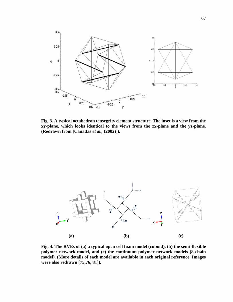
67

Fig. 3. A typical octahedron tensegrity element structure. The inset is a view from the

xy-plane, which looks identical to the views from the zx-plane and the yz-plane.

(Redrawn from [Canadas et al., (2002)]).

(a) (b) (c)

Fig. 4. The RVEs of (a) a typical open cell foam model (cuboid), (b) the semi-flexible

polymer network model, and (c) the continuum polymer network models (8-chain

model). (More details of each model are available in each original reference. Images

were also redrawn [75,76, 81]).

68

Table 1. Summary of the cytoskeleton models

Models Principle (how to

model) Advantage/Disadvantage Ref

Cel

l-S

cale

Conti

nuum

Model

(~ 1

0

m)

Elastic/Viscoel

astic Model

Cytopla

sm as

continu

ous

media

Constitut

ive

rheologic

al

equation Good for

cell

dynamics

simulation/

No

microstruct

ural

information

Computationall

y efficient

enough to

describe the

near

equilibrium/tran

sient behaviors

of cell

dynamics.

[13,3

6]

Multiphasic

Model

Constitut

ive

rheologic

al

equation

s in each

phase

More accurate

at the cost of

computational

cost

[41]

Soft Glassy

Model

Sollich’s

equation

Prediction over

large time scale

ranges

[51]

Str

uct

ure

-bas

ed P

re-S

tres

s M

odel

(4~

10

m)

Cortical

Model, Cable

Nets Model

Pre-

stressed

stress

unit

Cable

networks

Pre-

stressed is

considered.

Possibility

for both

cell

dynamics

and cell

properties.

Lack of

polymer

structural

information

(semi-

flexibility)

Lack of

microtubule and

intermediate

filament

information

[57,5

6]

69

Table 1. Summary of the cytoskeleton models (cont.)

Tensegrity

Model

Pre-

stressed

stress

unit

Cable-

Strut

networks

Pre-stressed

is

considered.

Possibility

for both cell

dynamics

and cell

properties.

Lack of

polymer

structural

information

(semi-

flexibility)

Considers all

actin

filaments,

microtubules,

and

sometimes

intermediate

filaments.

Versatility of

the model

[56] S

truct

ure

-bas

ed S

emi-

Fle

xib

ilit

y M

odel

(1~

4

m)

Open Cell

Foam

Model

Stress

unit with

semi-

flexibilit

y

Rigid

beam

structure Semi-

flexibility or

bending is

considered.

Lack of

microtubule

and polymer

molecule

information

(network

morphology)

. Generally,

not good for

cell

dynamics

Prediction of

bending

dominated

deformation.

Some

structural

information is

not correct.

[30,31

]

Semi-

flexibility

Network

Element

Model

Simplified

Polymer

Network

Complex

network

behavior is

well

simplified.

Lack of 3D

structural

information

[30]

Continuu

m

Polymer

Network

Model

Continuou

s medium

with

principal

axes

Continuum

mechanics

and

microstructura

l strain-stretch

relation are

connected.

Possibility for

cell dynamics

[81,84

]

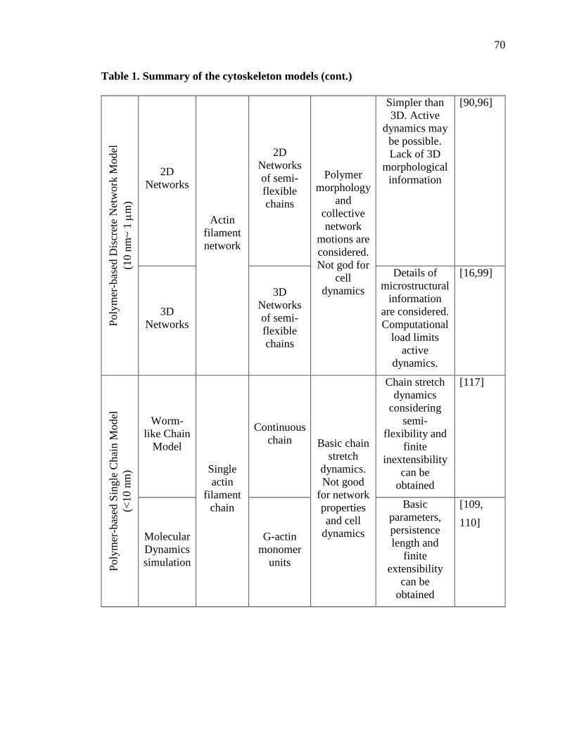
70

Table 1. Summary of the cytoskeleton models (cont.)

Poly

mer

-bas

ed D

iscr

ete

Net

work

Model

(10 n

m~

1

m)

2D

Networks

Actin

filament

network

2D

Networks

of semi-

flexible

chains

Polymer

morphology

and

collective

network

motions are

considered.

Not god for

cell

dynamics

Simpler than

3D. Active

dynamics may

be possible.

Lack of 3D

morphological

information

[90,96]

3D

Networks

3D

Networks

of semi-

flexible

chains

Details of

microstructural

information

are considered.

Computational

load limits

active

dynamics.

[16,99]

Poly

mer

-bas

ed S

ingle

Chai

n M

odel

(<10 n

m)

Worm-

like Chain

Model

Single

actin

filament

chain

Continuous

chain Basic chain

stretch

dynamics.

Not good

for network

properties

and cell

dynamics

Chain stretch

dynamics

considering

semi-

flexibility and

finite

inextensibility

can be

obtained

[117]

Molecular

Dynamics

simulation

G-actin

monomer

units

Basic

parameters,

persistence

length and

finite

extensibility

can be

obtained

[109,

110]

71

ACKNOWLEDGEMENT

The partial financial support from the Energy Research & Development Center of

Missouri University of Science & Technology is gratefully acknowledged.

72

REFERENCES

1. D. Discher, C. Dong, J. J. Fredberg, F. Guilak, D. Ingber, P. Janmey, R. D. Kamm, G.

W. Schimd-Scho and S. Weinbaulam, Ann. Biomed. Eng., 37, 847 (2009).

2. J. R. Stehn, N. K. Haass, T. Bonello, M. Desouza, G. Kottyan, H. Treutlein, J. Zeng, P.

R. B. B. Nascimento, V. B. Sequeira, T. L. Butler, M. Allanson, T. Fath, T. A. Hill, A.

McCluskey, G. Schevzov, S. J. Palmer, E. C. Hardeman, D. Winlaw, V. E. Reeve, I.

Dixon, W. Weninger, T. P. Cripe, and P. W. Gunning, Cancer Res, 73, 5169 (2013).

3. S. D. Bernal, S. B. Baylin, J. H. Shaper, A. F. Gazdar, and L. B. Chen Cancer Res, 43,

1798 (1983).

4. F. C. S. Ramaekers and F. T. Bosman, J. Pathol., 201, 351 (2004).

5. B. Geiger, J. Spatz, and A. Bershadsky, Nat. Rev. Mol. Cell Biol., 10, 21 (2009).

6. M. Mehrbod and M. R. K Mofrad , PLoS ONE, 6, 10, e25627 (2011).

7. E. M. Huisman, in Introduction, Simulation of biopolymer networks under shear,

Leiden University, Leiden (2011).

8. M. E. Chicurel, C. S. Chen, D. E. Ingber, Curr. Opin. Cell Biol., 10, 232 (1998).

9. N. Wang, K. Naruse, D. Stamenovic, J. J. Fredberg, S. M. Mijailovich, I. M. Tolic-

Norrelykke, P. Natl. Acad. Sci. USA, 98, 7765 (2001).

10. D. E. Ingber, J. Cell Sci., 116, 1157 (2003)

11. C. Galli, S. Guizzardi, G. Passeri, G. M. Macaluso, R. Scandroglio, Acta Biomedica.,

76, 5 (2005).

12. T. J. Chen, C. C. Wub, F. C. Su, Med. Eng. Phys., 34, 1375 (2012).

13. M. R. K. Mofrad, Annu. Rev. Fluid Mech. 41, 433 (2009).

14. H. Lodish, A. Berk, S. L. Zipursky, P. Matsudaira, D. Baltimore, and D Darnell,

Molecular Cell Biology, W.H. Freeman Co. publications, New York (1999).

15. F. Gittes, B. Mickey, J. Nettleton, and J Howard, J. Cell Biol., 120, 923 (1993).

73

16. T. Kim, W. Hwang and R.D. Kamm, Exp. Mech., 49, 91 (2009).

17. M. L. Gardel, J. H. Shin, F. C. MacKintosh, L. Mahadevan, P. A. Matsudaira, and D.

A. Weitz, Science, 304, 1301 (2004).

18. M. L. Gardel, J. H. Shin, F. C. MacKintosh, L. Mahadevan, P. A. Matsudaira, and D.

A. Weitz, Phys. Rev. Lett., 93, 188102 (2004).

19. F. C. MacKintosh, J. Kas, and P. A. Janmey, Phys. Rev. Lett., 75, 4425 (1995).

20. C. Storm, J. J. Pastore, F. C. MacKintosh, T. C. Lubensky and P. A. Janmey, Nature,

435, 191 (2005).

21. J. Xu, Y. Tseng, and D. Wirtz, J. Biol. Chem. 275, 35886 (2000).

22. O. Lieleg, M. M. A. E. Claessen, and A. R. Bausch, Soft Matter, 6, 218 (2010).

23. B. Alberts, D. Bray, A. Johnson, J. Lewis, M. Raff, K. Roberts, P. Walter, in Essential

cell biology : An introduction to the molecular biology of the cell, Garland Publishing,

New York (1998).

24. I. Fujiwara, S. Takahashi, H. Tadakuma, T. Funatsu, S. Ishiwata, Nat. Cell Biol., 4, 666

(2002).

25. G. A. Buxton, N. Clarke, P. J. Husse, Express Polym. Lett., 3, 579 (2009).

26. T. Mitchison and M. Kirschner, Nature, 312, 237 (1984).

27. D. Stamenović, FME Transactions, 34, 57 (2006).

28. M. J. Unterberger and G. A. Holzapfel, Biomech. Model Mechanobiol., 13, 1155 (2014)

29. J. Chen, Interface Focus, 4, 20130055 (2014)

30. T.J. Chen, C.C. Wu, and F.C. Su, Med. Eng. Phys., 34, 1375 (2012)

31. M. M. Nava, M. T. Raimondi, and R. Pietrabissa, Biomech. Model Mechanobiol., 13,

929, (2014).

32. E. Moeendarbary, and A. R. Harris, WIREs Syst. Biol. Med., 6, 371, (2014).

74

33. S.S. Andrews, Phys. Biol., 11, 011001 (2014)

34. E. Roberts, Cur. Opin. Struc. Biol., 25, 86 (2014)

35. P. A. Janmey, and C. Schmidt, in Cytoskeletal Mechanics - Models and Measurements

in Cell Dynamics, M. R. K. Mofrad, and R. D. Kamm Eds., Cambridge University Press

(2006).

36. M. R. K. Mofrad, H. Karcher, and R. D. Kamm, in Cytoskeletal Mechanics - Models

and Measurements in Cell Dynamics, M. R. K. Mofrad, and R. D. Kamm Eds.,

Cambridge University Press (2006).

37. B. Fabry, G. Maksym, J. Butler, M. Glogauer, D. Navajas, J Fredberg, Phys. Rev. Lett.,

87, 148102 (2001).

38. A. R Bausch, F. Zeimann, A. A. Boulbitch, K. Jacobson, E. Sackmann, Biophysics, 75,

2038 (1998).

39. D. Aubry, H. Thiam, M. Piel, and R. Allena, Biomech. Model. Mechanobiol., DOI

10.1007/s10237-014-0595-3 (2014)

40. I. Pajic-Lijakovic and M. Milivojevic, Biomech. Model Mechanobiol., 13, 1097 (2014)

41. F. Guilak, M. A. Haider, L. A. Setton, T. A. Laursen, and F. P.T. Baaijens, in

Cytoskeletal Mechanics - Models and Measurements in Cell Dynamics, M. R. K.

Mofrad, and R. D. Kamm Eds., Cambridge University Press (2006).

42. V.C. Mow, S.C. Kuei, W.M. Lai, and C.G. Armstrong, J. Biomech. Eng., 102, 73

(1980).

43. W.M. Lai, J.S. Hou, and V.C. Mow, J. Biomech. Eng., 113, 245 (1991).

44. W.Y. Gu,W.M. Lai, and V.C. Mow, J. Biomech. Eng., 120, 169 (1998).

45. M. Biot, J. Appl. Phys. 12, 155 (1941).

46. A.F. Mak, J. Biomech. Eng., 108, 123 (1986).

47. M.R. DiSilvestro and J.K. Suh, An. Biomed. Eng., 30, 792 (2002).

48. F.P.T. Baaijens, W.R. Trickey, T.A. Laursen, and F. Guilak, An. Biomed Eng., 33, 494

(2005)

75

49. L. Cao, F. Guilak, and L. Setton, Cell. Mol. Bioeng., 2, 306 (2009).

50. B. Fabry and J. J. Fredberg in Cytoskeletal Mechanics - Models and Measurements in

Cell Dynamics, M. R. K. Mofrad, and R. D. Kamm Eds., Cambridge University Press

(2006).

51. B. Fabry and J. J. Fredberg, Respir. Physiol. Neurobiol, 137, 109 (2003).

52. P. Sollich, F. Lequeux, P. Hebraud and M. Cates, Phys. Rev. Lett., 78, 2020 (1997).

53. P. Sollich, Phys. Rev. E, 58, 738 (1998).

54. Haider M, Guilak F, J Biomech Eng., 122, (3), 236 (2000)

55. Haider M, Guilak F, J Biomech Eng 124, (5), 586 (2002)

56. D. Stamenović in Cytoskeletal Mechanics - Models and Measurements in Cell

Dynamics, M. R. K. Mofrad, and R. D. Kamm Eds., Cambridge University Press (2006).

57. D. V. Zhelev, D. Needham, R. M. Hochmuth, Biophys. J., 67, 696 (1994).

58. D.E. Discher, D.H. Boal, and S.K. Boey, Biophys. J., 75, 1584 (1998).

59. S.K. Boey, D.H. Boal, and D.E. Discher, Biophys. J., 75: 1573 (1998).

60. D. Stamenovic´, D. E. Ingber, Biomech. Model Mechanobiol., 1, 95 (2002).

61. M. F. Coughlin and D. Stamenović, Biophys J, 84, 1328 (2003).

62. R. Paul, P. Heil, J. P. Spatz, and U. S. Schwarz US, Biophys J, 94, 1470 (2008).

63. K. Y. Volokh, and O. Vilnay, Int. J. Solids Struct., 34, 1093 (1997).

64. D.E. Ingber, L. Dike, L. Hansen, S. Karp, H. Liley, and A. Manitos, Int. Rev. Cytol.,

150, 173 (1994).

65. D. Stamenović, and M. F. Coughlin, J. Theor. Biol., 201, 63 (1999).

66. F. J. Alenghat, B. Fabry, K. Y. Tsai, W. H. Goldmann and D. E. Ingber, Biochem.

Biophys. Res. Commun., 277, 93 (2000)

76

67. J. M. Vasiliev, J. Cell Sci. Suppl., 8, 1 (1987).

68. D. E. Ingber, Annu. Rev. Physiol., 59, 575 (1997).

69. B. Fuller, Portfolio & ARTnews Annual, 4, 112 (1961).

70. H. Baudriller, B. Maurin, P. Canadas, P. Montcourrier, A. Parmerggiani, and N.

Betache, C R Mecanique, 334, 662 (2006).

71. P. Canadas, V.M. Laurent, C. Oddou, D. Isabey, and S. Wendling, J Theor Biol., 218,

155 (2002).

72. N. Wang and D. Stramenovic, Am. J. Physiol. Cell Physiol., 279, C188 (2000).

73. D.E. Ingber, FASEB J., 20, 811 (2006).

74. Y.Z. Luo, X. Xu, T. Lele, S. Kumars, and D.E. Ingber, J. Biomech., 41, 2379 (2008).

75. R. Satcher, C. F. Dewey Jr, and J. H. Hartwig, Microcirculation, 4, 439 (1997).

76. S. Roy and H. J. Qi, Phys. Rev. E., 77, 061916 (2008).

77. P.J. Flory and J. Rehner Jr, J. Chem Phys., 11, 512 (1943).

78. L.R.G. Treloar, Trans. Far. Soc., 42, 83 (1946).

79. E.M. Arruda, and M.C. Boyce, J. Mech. Phys. Solids, 41, 389 (1993).

80. P.D. Wu and E. Giessen, J. Mech. Phys. Solids, 41, 427 (1993).

81. J.S. Palmer and M.C. Boyce, Acta Biomater, 4, 597 (2008)

82. H. Van Oosterwyck, J.F. Rodriguez, M. Doblare, J.M. Garcia, Comput. Methods

Biomech. Biomed. Eng., 16, 1002 (2013).

83. G.A. Holzapfel, M.J. Unterberger, R.W. Ogden, J. Mech. Behav. Biomed. Mater., 38,

78 (2014)

84. M.J. Unterberger, K.M.Schmoller, A.R. Bausch, G.A. Holzapfel, J. Mech. Behav.

Biomed. Mater., 22, 95 (2013)

77

85. M.J. Unterberger, K.M.Schmoller, C. Wurm, A.R. Bausch, G.A. Holzapfel, Acta

Biomater., 9, 7343 (2013)

86. C.P. Broederz, C. Storm, F.C. MacKintosh, Phys. Rev. let., 101, 118103 (2008).

87. T.J. Chen, C.C. Wu, M.J. Tang, J.S. Huang, and F.C. Su, PloS One, 5, e14392 (2010).

88. F.C. MacKintosh, in Cytoskeletal Mechanics - Models and Measurements in Cell


89. P. A. Janmey, M. E. McCormick, S. Rammensee, J. L. Leight, P. C. Georges, and F. C.

MacKintosh, Nature Mater., 6, 48 (2007).

90. D. A. Head, A. J. Levine, and F. C. MacKintosh, Phys. Rev. Lett., 91, 108102 (2003).

91. D. A. Head, A. J. Levine, and F. C. MacKintosh, Phys. Rev. E Stat. Nonlin. Soft Matter

Phys., 68, 061907 (2003).

92. J. Wilhelm and E. Frey, Phys. Rev. Lett., 91, 108103 (2003).

93. P.R. Onck, T. Koeman, T. van Dillen, and E. van der Giessen, Phys. Rev. Lett., 95,

178102 (2005).

94. E. Conti and F.C. MacKintosh, Phys. Rev. Lett., 102, 088102 (2009).

95. A.S. Abhilash, P.K. Purohit, and S.P. Joshi, Soft Matter, 8, 7004 (2012).

96. R. Alonso, J. Young, and Y. Cheng, Cell. Mol. Bioeng., 7, 58 (2014)

97. F. Cucker, F., and S. Smale. IEEE Trans. Automat. Control, 52, 852 (2007).

98. B. Fallqvist, A. Kulachenko, and M. Kroon, J. Theor. Biol., 350, 57 (2014)

99. E.M. Huisman, T. van Dillen, P.R. Onck, and E. van der Giessen, Phys. Rev. Lett., 99,

208103 (2007).

100. E.M. Huisman, C. Storm, G.T. Barkema, Phy. Rev. E, 78, 051801 (2008).

101. E.M. Huisman, C. Storm, G.T. Barkema, Phys. Rev. E, 82, 061902 (2010).

102. T. Kim, W. Hwang, H. Lee, R. D. Kamm, PLoS Comput. Biol., 5, e1000439 (2009).

78

103. T. Kim, in Thesis: Simulation of Actin cytoskeleton structure and rheology,

Massachusetts Institute of Technology, Massachusetts, (2007).

104. T. Kim, M.L. Gardel, and E. Munro, Biophys. J., 106, 526 (2014).

105. M. Mak, M. Zaman, and R. Kamm, Med. Phys., 41, 164 (2014).

106. C. Cyron, A.R. Baush, K.W. Muller, and W.A. Wall, J. Comput. Phys., 244, 236

(2013).

107. J. Gong, D. Zhang, Y. Tseng, B. Li, D. Wirtz, and B.W. Scahfer, PLoS ONE, 8, e77417

(2013).

108. B. Li, Y. Wang, and J. Gong, J. Zhejiang Univ-Sci. A, 15, 732 (2014)

109. S. Matsushita, T. Adachi, Y. Inoue, M. Hojo, and M. Sokabe, J. Biomech., 43, 3162

(2010).

110. J-W. Chu and G. A. Voth, Biophys. J., 90, 1572 (2006).

111. O.N. Yogurtcu, J.S. Kim, and S.X. Sun, Biophys. J., 103, 719 (2012).

112. J. Fan, M.G. Saunders, and G.A. Voth, Biophys. J., 103, 1334 (2012).

113. J. Fan, M.G. Saunders, E.J. Haddadian, K.F. Ffreed, E.M. de la Cruz, and G.a. Voth,

J. Mol. Biol., 425, 1225 (2013).

114. D. Ming, Y. Kong, Y. Wu, and J. Ma, PNAS, 100, 104 (2003).

115. O. Kratky and G. Porod, Recl. Trav. Chim. Pays-Bas., 68, 1106 (1949).

116. M. Fixman and J. Kovac, J. Chem. Phys., 58, 1564 (1973)

117. G.A. Holzapfel and R.W. Ogden, J. Elast., 104, 319 (2011).

118. J.R. Blundell and E.M. Terentjev, Macromolecules, 42, 5388 (2009)

119. Y. Lin, X. Wei, J. Qian, K.Y. Sze, and V.B. Shenoy, J. Mech. Phys. Solids, 62, 2 (2014)

120. B. Wagner, R. Tharmann, I. Haase, M. Fischer, and A. R. Bausch, PNAS, 103, 13974

(2006).

79

121. H. Hatami-Marbini and M. R. K. Mofrad, Stud. Mechanobiology Tissue Eng.

Biomater., 4, 3 (2011).

122. G.A. Buxton, N. Clarke, and P.J. Hussey, eXPRESS Pol. Lett., 3, 579 (2009).

123. R. Alonso, J. Young, and Y. Cheng, Cell. Mol. Bioeng., 7, 58 (2014).

124. A. E. Likhtman, J. Non-Newtonian Fluid Mech. 157, 158 (2009).

125. J. Park, D.W.Mead, and M.M. Denn, J. Rheol. 56, 1057 (2012).

126. G. H. Pollack, in Cytoskeletal Mechanics - Models and Measurements in Cell


127. B. Maurin, P. Canadas, H. Baudriller, P. Montcourrier, and N. Bettache, J. Biomech.,

41, 2036 (2008).

128. P. Chen and V.B. Shenoy, Soft Matter, 7, 355 (2011).

129. S. Na, G.A. Meininger, and J.D. Humphrey, J. Theor. Biol., 246, 87 (2007).

130. Y. Jang, S. Park, and K.Char, Kor. J. Chem. Eng., 28, 1149 (2011).

131. Y. Jeong and I.S. Kang, Kor. J. Chem. Eng., 12, 540 (1995)

80

II. A constitutive model for entangled polymers incorporating binary

entanglement pair dynamics and a configuration dependent friction coefficient

Synopsis

Following recent work [e.g. Park et al. (2012) J. Rheol. 56: 1057-1082, Yaoita et

al. (2012) Macromolecules 45: 2773-2782, Ianniruberto et al. (2012) Macromolecules 45:

8058-8066] we introduce the idea of a conFig.uration dependent friction coefficient (CDFC)

based on the relative orientation of Kuhn bonds of the test and surrounding matrix chains.

We incorporate CDFC into the “toy” model of Mead et al. (1998) [Macromolecules 31:

7895-7914] in a manner akin to Yaoita et al. (2014) [Nihon Reoroji Gakkaishi, 42: 207-

213]. Additionally, we incorporate entanglement dynamics (ED) of discrete entanglement

pairs into the new Mead-Banerjee-Park (MBP) model in a way similar to Ianniruberto and

Marrucci, (2014) [J. Rheol. 58: 89-102]. The MBP model predicts a deformation dependent

entanglement microstructure which is physically reflected in a reduced modulus that heals

slowly following cessation of deformation. Incorporating ED into the model allows “shear

modification” to be qualitatively captured. The MBP model is tested against experimental

data in steady and transient extensional and shear flows. The MBP model captures the

monotonic thinning of the extensional flow curve of entangled monodisperse polystyrene

(PS) melts [Bach et al. (2003) Macromolecules 36: 5174-5179] while simultaneously

predicting the extension hardening found in PS semi-dilute solutions where CDFC is

diluted out [Bhattacharjee et al. (2002) Macromolecules 35: 10131-10148].

81

The simulation results also show that the rheological properties in nonlinear

extensional flows of PS melts are sensitive to CDFC but not to convective constraint

release (CCR) while those for shear flows are influenced more by CCR. The monodisperse

MBP “toy” model is generalized to arbitrary polydispersity.

82

I. INTRODUCTION

The idea of a configuration dependent friction coefficient (CDFC), which is based

on the relative orientation of a test chain segment to the surrounding matrix chain segments,

was previously introduced by [Park et al. (2012)]. Although related through a Kuhn-Grün

analysis [e.g. Larson (1988)], a better, more fundamentally based proposition is to base

CDFC on the relative orientation of the Kuhn bonds of the test and matrix chains

respectively [Ianniruberto et al. (2011, 2012); Yaoita et al. (2012, 2014)]. Since CDFC

impacts both the stretch (Rouse) and terminal relaxation times equally, CDFC can in

principle capture the monotonic thinning of the extensional flow curve of entangled

monodisperse polystyrene (PS) melts [Bach et al. (2003)] while simultaneously predicting

the extension hardening found in entangled monodisperse PS solutions where the effects

of CDFC is negligible due to dilution [Bhattacharjee et al. (2002); Desai and Larson

(2014)].

In addition to altering the form of CDFC employed we shall also address other

fundamental issues in molecular modelling the rheology of polymer melts. In particular,

the mono and polydisperse MLD models (Mead-Larson-Doi model [Mead et al. (1998)])

assume a constant entanglement density in all flow situations. This fundamental

assumption is almost certainly wrong. Theoretically, the assumption of a constant

entanglement density is reflected in the fact that the equilibrium plateau modulus is used

to scale the stress in all tube models, i.e. the GLaMM model [Graham et al. (2003)], all

Doi-Edwards type models such as the MLD model [Mead et al. (1998); Mead (2007)], and

the pom-pom model [McLeish and Larson (1998)]. It’s difficult to understand how the

83

equilibrium plateau modulus can be used to scale stress levels in the highly nonlinear flow

regime since reductions in the entanglement density have been demonstrated in non-

equilibrium molecular dynamics simulations of shear flow [Baig et al. (2010)] and detailed

molecular models [Andreev et al. (2013)]. Additionally, interrupted transient step shear

rate rheological data on linear and long-chain branched (LCB) polyethylene melts by Dealy

and Tsang (1981) [and references therein] strongly support the idea of a dynamic

entanglement network. These theoretical and experimental results suggest that a

fundamental re-appraisal is appropriate for the formulation of molecular constitutive

models that span the full range of flows from linear viscoelasticity to the nonlinear fast

flow regime of linear and LCB polymer melts.

In this paper we develop a new molecular model based on the dynamics of discrete

entanglement pairs (entanglement dynamics: ED) as opposed to traditional mean field tube

descriptions [Desai and Larson (2014)]. Adopting this description is supported by recent

atomistic simulations which reveal the nature of an entanglement to be that of a topological

coupling of a discrete pair of chains [Everaers et al. (2004); Tzoumanekas and Theodorou

(2006); Baig et al. (2010)]. Both the modulus and the terminal disengagement time are

functions of the entanglement density and changes to the entanglement density will directly

impact these quantities. This paper seeks to incorporate a quantitative description of

entanglement pair dynamics and a Kuhn bond based CDFC into the mono and polydisperse

MLD “toy” models. This will yield a general molecular constitutive model at the

theoretically and computationally simple “toy” level that can handle arbitrary

polydispersity in arbitrarily fast flows.

84

This paper is organized as follows: In Sec. II, we introduce a toy dynamical

equation for entanglement pairs in monodisperse systems. In Sec. IIA we define the

specific form of CDFC we shall use for monodisperse systems. Section III reviews aspects

of the Desai-Larson modified DEMG model (Doi-Edwards-Marrucci-Grizzuti [Pearson et

al. (1991), Mead and Leal (1995), Mead et al (1995)]) which will serve as a base case for

the current work. Section IV introduces two new effects we anticipate will impact the

dynamics of highly oriented systems. Section V summarizes the new monodisperse toy

molecular model incorporating all the features presented in Secs. II-IV. Steady and

transient uniaxial extension is simulated and compared with experimental data in Sec. VI.

Steady and transient simulations are also performed for shear flow in Sec. VIA. The results

of our new molecular model are discussed and summarized in Sec. VII.

85

II. MODELLING THE ENTANGLEMENT PAIR DYNAMICS FOR

MONODISPERSE SYSTEMS

We begin by constructing a toy dynamical equation for the number of

entanglements on a chain in a monodisperse melt. This is inspired by analogy to the slip-

link entanglement dynamics in the stochastic simulator [Park et al. (2012)] and the discrete

slip-link model of Andreev et al. (2013) and is similar in spirit to transient network models

[Mewis and Denn (1983)]. Ianniruberto and Marrucci (2014) have independently pursued

conceptually similar arguments to those presented below to construct a dynamical equation

for the entanglement density.

diffusiontipmatrix

d

e

anglementsentofndestructioconvective

tube

diffusiontipchaintest

d

e

t

tNNtN

ttS

t

tNNtN

11:

(1)

Here, tN , represents the number of entanglement pairs per polymer chain at the

current time, t while e

eM

MN represents the average equilibrium number of

entanglement pairs per chain of molecular weight M with entanglement molecular weight

eM . The non-equilibrium tube disengagement time is td

1 . In the second term on the

RHS, is a parameter that reflects the “efficiency” of the convective constraint release

mechanism (CCR). The velocity gradient is given by and the orientation tensor is defined

by RRStube

, where R

is the unit end-to-end vector of a tube segment. The relative

stretch of the “partially disentangled” chain variable is defined by tL

tLt

eq

where tL

86

is the current tube contour length and tLeq is the equilibrium length. Note here that t

is different from the relative stretch of a “fully entangled” chain relative to the initial

equilibrium length, which is defined as

eqL

tLt . Additionally, the ratio between the

maximum stretch ratios of both relative stretches is defined as

max

max

tt

.

What equation (1) represents is the idea that entanglements are destroyed by CCR

in proportion to the current entanglement density, tN , times the fractional rate at which

they are destroyed via convection. Entanglements are created by tip diffusion/fluctuations

of the test chain and the matrix chains at a rate in proportion to the difference between the

entanglement density and its equilibrium value, a driving force, divided by the time scale

for the process, td

1 .

We now derive the entanglement destruction term in (1), more specifically the

expression for the fractional rate of convective destruction of entanglements:

ttS

tube

: . Since tLeq

is a function of the entanglement density tN , i.e.

tNtLeq ~ (See equation A1.3 of Appendix A), differentiating tL

tLt

eq

with respect

to time and simplifying yields:

tt

tN

tN

t

t

tL

tL

tL

tL

mechanismsallviastretchtubeof

rateFractional

anglementdisentdrivenCRtoduecontourchaintheof

entsrearrangemInternal

eq

eq

2

1 (2)

87

The fractional rate of change of the tube contour length tL

tL has two separate

contributions. The first term on the RHS of (2) is new and represents the fractional tube

shortening/lengthening rate due to constraint release (CR) driven disentanglement. The

second term on the RHS represents the fractional rate of tube stretching due to affine stretch,

chain retraction of the chain tips into interior parts of the chain and CCR driven tube

shortening. All of the effects contained within the second term on the RHS have been

presented in Mead et al 1998 and discussed in detail there. Only the disentanglement term,

tN

tN

tL

tL

eq

eq

2

1 , is new. However, even this term is discussed in Sec. II.A.2 of Mead et al

1998. Note that in the original MLD model the entanglement density was assumed to be

constant, 0N .

From equation (16) or (29) we determine that

tN

tNt

2

1

so we finally have

an expression for tL

tL in terms of MBP model terms,

ttt

t

t

tN

tN

tL

tL

2

1 (3)

Thus, calculating tL

tL is straightforward in the MBP model. Equation (3) for tL

tL

can be used directly in equation (9) defining k of the MLD paper (Mead et al. 1998 pg.

7901);

tS

ttS

tL

tLSk

:::

(4)

88

Generally,

ttS

: which when valid reduces (4) to the same CCR

expression in the original MLD model. We use the expression for k (4) in the convective

destruction of entanglements term in (1) as well as in the stretch equation and orientational

relaxation equation, both of which include CCR, in the MBP model.

Note that we have ignored factors of 2 in the denominator of the reptative

diffusion entanglement creation/destruction terms in (1). We ignore this factor in light of

the fact that we are not considering contour length fluctuations explicitly. Contour length

fluctuations have no such factor scaling the diffusive creation/destruction of entanglements.

Tip contour length fluctuations are presumably responsible for most of the diffusive

entanglement creation/destruction processes. However, for the newly created tip

entanglement to diffuse into the interior of the chain it takes the reptation time. Hence using

the bare reptation time as a characteristic time scale for entanglement creation is a

compromise in this simple toy version of the model. A tube coordinate is needed to have a

proper description of the entanglement creation/destruction processes. The model of

Andreev et al. (2013) provides just such a description in a detailed way. Experimentally,

studies of the re-entanglement kinetics/dynamics from virgin (unentangled), nascent

polymer melts provide a viable means to quantitatively determine the appropriate time

scale for the re-entanglement processes described in equation (1) [Yamazaki et al (2006);

Rastogi et al (2003); Wang et al (2009)].

The factor scaling the convective destruction of entanglements term represents

a CCR “efficiency” factor related to the number of constraint release events required to

generate a single disentanglement [Ianniruberto and Marrucci (1996)].

89

This interpretation suggests that 10 . The factor was originally introduced

by Ianniruberto and Marrucci (1996, 2001) to ensure a stable monotonic steady shear stress

vs. shear rate curve and retains this interpretation in the current work.

The non-equilibrium tube disengagement time td

1 is a function of the

entanglement density, tN . Physically this arises because the absolute distance for the

chain to diffuse shortens as the number of entanglements decreases. In Appendix A we

derive the result:

tN

tNt d

e

d 0,

1

(5)

Here td

1 is the terminal tube disengagement time for arbitrary tN relative to the non-

equilibrium tube disengagement time, td 0, , which will be lowered in fast flows by CDFC

and hence is also a function of time (Sec. IIA).

Using (5) in (1) the expression for the entanglement dynamics can now be

simplified and re-written as:

ndestructionglemententainducedCCR

tube

diffusiontipviacreationanglementent

e

d

e tNtt

StN

N

t

NtN

:1

2

0,

(6)

Note that the MLD “toy” model for ED does not explicitly contain tip fluctuations

which are undoubtedly very important in the re-entanglement process [Mead (2011b);

90

Andreev et al. (2013)]. A more detailed model at the tube coordinate level is needed to

properly capture the effects of tip fluctuations versus reptational effects.

The modulus scales the stress in molecular models and is a function of the

entanglement density. It can be written as [Dealy and Wissbrun (1989)]:

0

N

ee

N GN

tN

tN

M

RT

tM

RTtG

(7)

Here, 0

NG is the equilibrium plateau modulus. , R, and T are density, gas constant,

and absolute temperature, respectively. If the entanglement density is significantly lower

than equilibrium the modulus will be directly impacted (lowered) for an extended period

of time following deformation. This could explain the phenomena of “shear modification”

which is still unexplained theoretically [Rokudai (1979); Yamaguchi and Wagner (2006);

Leblans and Bastiaansen (1989)]. Shear modification is a deformation-induced reversible

reduction in the dynamic moduli for high molecular weight polydisperse linear and LCB

entangled polymers [Dealy and Wissbrun (1989)]. Shear modification is one of the last

great unsolved theoretical problems in nonlinear molecular rheology.

One of the conundrums with the above entanglement dynamics model is that in

very fast extension virtually all the entanglements are convected away leaving a modulus

that approaches zero. Not surprisingly the discrete slip-link model by Andreev et al. (2013)

has similar issues. When all entanglements are stripped from the chain the Peterlin modulus

will be applicable [Desai and Larson (2014)]. The Peterlin modulus is that of an

unentangled ensemble of stretched chains in a flow field.

91

A. Formulation of the expression for Kuhn bond based CDFC on the stretch and

terminal orientational relaxation times

Here we briefly outline how to calculate the net fractional Kuhn bond orientation

and the reformulated expression for the decrease in the friction coefficient due to net Kuhn

relative bond alignment of the test chain with respect to the matrix chains. Note here that

structural parameters of PS are used since the experimental data of PS melts and solutions

are compared with the predictions by various models studied in this paper.

We start by denoting the net Kuhn bond orientation in the polydisperse MLD “toy”

model single segment asKuhn

S . The net Kuhn bond orientation of the matrix is proportional

to the birefringence which, using the freely jointed chain model in a Kuhn-Grün analysis,

yields:

termsisotropicRRx

xtermsisotropicS

x

xS

tubeKuhn

11 L

31

L

31 (8)

Where tube

S is the single tube segment orientation. The inverse Langevin function term, L-

1(x), in (8) can be accurately approximated within 1% [Treloar (1975) pg. 178] for easy

calculation,

642

1 5

1

5

1

5

3

L

31 xxx

x

x

(9)

where x is the fractional chain extension:

max

x (10)

92

Note here that Yaoita et al. (2012) use the simplest approximation

2

1L

31 x

x

x

in their work. It is also noted that the definition of x will be altered,

max

x , for models

that include entanglement density dynamics.

The maximum relative stretch max is calculated as [Mead (2011b)],

2/1

0

2/1

max 82.0

JMC

Mn e . (11)

Here J is the number of carbon-carbon sigma bonds in the backbone, J=2 for PS,

eM is the equilibrium average entanglement molecular weight (13333 Da for PS). In non-

equilibrium flow situations the entanglement molecular weight is a function of

concentration and the dynamic entanglement density along the chain. C is the

characteristic ratio, 9.8 for PS [Flory (1969)] and 0M is the monomer molecular weight,

104 Da for PS. n is the number of Kuhn bonds in an entanglement segment. Note that for

PS melts 2.4max , a relatively small maximum stretch. The maximum stretch will be

much larger ( 25max ) for the entangled high MW entangled PS solutions considered by

Bhattacharjee et al. (2002).

Ianniruberto et al. calculated the functional form of the reduced friction versus

matrix Kuhn bond orientation for monodisperse PS melts in their 2012 paper [Ianniruberto

et al. (2012) see Fig. 4]. We use the Ianniruberto et al. (2012) CDFC calculation as a guide.

93

65.1

,,

0,02239.0

tS

tttKuhn

eqs

s

eqd

d

eq

1.0KuhnS (12)

Where is the monomeric friction coefficient, d is the reptation time, and s is

the longest Rouse relaxation time. Subscript “eq” indicates equilibrium value and “0”

means a value for a fully entangled chain.

The true form of the dependence of the accelerated relaxation rate can in principle

be determined by the nonlinear extensional stress relaxation experiments of Yaoita et al.

(2012) which are of fundamental importance with respect to CDFC. These experiments

are discussed in detail in Section III and Fig. 7.

Following Yaoita et al. (2012) we define the scalar net fractional Kuhn bond

alignment KuhnS as,

tubepKuhn SxxxS

642

5

1

5

1

5

3 10 KuhnS (13)

The fractional Kuhn bond orientation,KuhnS , varies between zero and one for

perfect orientation. The anisotropic tube orientation in uniaxial extension is denoted by

yyxxtube

SSS . For shear deformation the principal values must be used,

21

224 xyyyxxtube

SSSS . The mass fraction of polymer scales the fractional Kuhn bond

orientation and is represented by p such that CDFC for both melts, 1p , and entangled

solutions, 1p , can be modelled.

94

III. MODIFICATION OF THE DESAI-LARSON TOY DEMG MODEL TO

INCORPORATE ED, CDFC AND CCR

Here we briefly outline how to incorporate the new results in Sections II and IIA

into the Desai-Larson modified DEMG model [Desai and Larson (2014)]. We eliminate

the Desai and Larson tube dilation effect and replace it with the CDFC and entanglement

dynamics results presented in Sections II and IIA above. This allows both the

disengagement time and the stretch time to be modified by CDFC which should in principle

allow an accurate modeling of steady state extensional viscosity data for both melts and

solutions.

One of the key theoretical developments in the Desai-Larson model is the

derivation of a new stretch dynamics equation for the partially disentangled chain that

incorporates the fact that the maximum extension is a function of the entanglement density

[Mead (2011b)]. When tN

MtM e changes (increases) with deformation induced

disentanglement, the maximum stretch also increases as described below.

2/1

0

2/1

0

2/1

max 82.082.0

JtNMC

MJ

MC

tMnt e

(14)

There is one new stretching effect to account for in the stretch equation: stretch

shortening due to removal of chain back folds. The stretch dynamical equation for the

diluted (partially disentangled) chain, generalized to include constraint release effects, is

[Desai and Larson (2014), Mead et al. (1998)].

95

shorteningtubedrivenCCR

dtube

retractionchain

s

s

stretchaffine

tube

nglementdisentatoduereductionstretch

t

tSkS

tt

12

1:1

2

11:

(15)

where,

2

1

max

max

tN

Ntt e

and tNtNNt e

2

3

2

1

2

1 (16)

and the nonlinearity of the spring is incorporated in a single factor denoted by sk [Cohen

(1991), Desai and Larson (2014)]:

1/13

/3

3

L

22

max

22

max

222

max

222

max

max

max

1

t

t

t

t

tk s (17)

We have added a CCR tube shortening term to the Desai-Larson stretch equation

(15) that requires discussion. This is done in Section IV below.

The above generalized expression of the stretch dynamics is principally what we

take from the Desai-Larson diluted tube model. We use the entanglement dynamics model

presented in Section II to replace the tube dilation dynamics expressions in the Desai-

Larson model.

96

IV. MODIFICATION OF THE NEW CDFC-ED “TOY” MLD MODEL TO

ACCOUNT FOR REDUCED LEVELS OF CCR FOR HIGHLY ALIGNED

SYSTEMS

In this Section we outline the manner in which the previously presented model can

be modified to account for the idea that CCR effects are different (greatly reduced) in

systems of slightly oriented versus highly oriented chains. These effects will impact CCR

driven re-orientation as well as CCR driven stretch relaxation (tube shortening) in fast

flows [Mead et al. (1998)]. These ideas are partly motivated by the work of Desai and

Larson (2014) that showed that CCR appears not to be important to capture the salient

features of fast nonlinear extensional flows. This is a conclusion that we affirm in

calculations with our new model.

The specific effect we wish to incorporate in our model is that CCR effects do not

strongly impact highly aligned chains. For example, in the limit of perfectly aligned chains

in fast flow there are no dynamical (topological) constraints and consequently CCR will

have no effect on the orientation or stretch of the test chain even though tube

S: is very

large [Desai and Larson (2014)]. Of course this ideal limiting situation can only be

approached in any finite deformation rate flow. We propose an ad hoc empiricism that

smoothly transits between the Gaussian and highly oriented extreme situations. A sketch

of these ideas for CCR driven stretch relaxation is shown in Fig.s 1 and 2.

We propose the following empirical changes to the stretch and orientation

dynamical equations to account for the ideas presented in the above thought experiment.

CCR in stretching flows relaxes 12

1 of the stretch associated with a given

97

entanglement [Mead (2011a)]. Using the above ideas, we construct an empirical function

that smoothly transits between the Gaussian and highly oriented cases.

112

11

2

11

2

1

tube

shorteningtubebiasedorientedhighly

tube

shorteningtubeGaussian

SS

(18)

We have included a new empirical term to the tube shortening expression,

tube

S1 . Fig. 1 illustrates the physical ideas underlying this empirical factor multiplying

the tube shortening term. Note that for 1tube

S we assume the chain is unraveled and

linear rather than a zig-zagged cat’s cradle (back folded) conformation. The new term

effectively wipes out tube shortening stretch relaxation for fast flows where the tube is

highly oriented. Desai and Larson (2014) have shown that this is a desirable feature to have

in the model for fast uniaxial extension and this underlies the motivation for this ad hoc

factor in the stretch equation.

Incorporating the new proposed physics into the stretch equation yields:

t

tSSkStt

dtubetube

s

stube 12

1:11

2

11:

(19)

Thus, at high fractional extensions the effect of CCR on stretch smoothly disappears

as tube

S monotonically increases. Thus, CCR can effectively reduce stretch in shear flows

where the orientation is lower than it is in extensional flows.

98

We also propose an ad hoc modification to the orientation dynamics equation to

account for biased (reduced) re-orientation due to nematic (molecular packing) effects in

highly aligned systems. Nematic effects are well established in cross-linked rubbers and

polymer melts [Doi et al. (1989)]. In such highly oriented systems the switch function,

1,

already diminishes the effect of CCR on the re-orientation process. We add to this effect

with an ad hoc empirical nematic re-orientation suppression factor KuhnS1 .

t

tS

ttS

t dtube

dKuhn 1212

1:

111

1

(20)

The factor KuhnS1 empirically accounts for the idea that the re-orientation process

will be biased (reduced) by nematic packing effects due to the net Kuhn bond orientation

of the matrix. Note that we are actually not including a biased re-orientation but rather an

increased orientational relaxation time which has a similar effect on the orientation level.

Another way to look at this effect is that constraint release effects will be ineffectual in

highly aligned systems i.e. when KuhnS is large (see Fig.s 1 and 2). Including the new factor

of KuhnS1 along with the switch function will effectively reduce all CCR driven re-

orientation in fast stretching flows where KuhnS is large.

Note that there will be a sharp distinction between uniaxial extension and shear

with the above two modifications. In uniaxial extension the orientation and stretch is severe

and the above two modifications will both kick in. Conversely, in shear flows the

orientation and stretch is weak and 11 KuhnS such that there are no nematic effects in

melts or solutions.

99

V. SUMMARY OF THE EQUATIONS IN THE EDS - KUHN BOND CDFC RE-

FORMULATION OF THE MONODISPERSE MLD TOY MODEL

Here we briefly summarize the equation set for the new monodisperse MLD “toy”

model [see Desai and Larson (2014) equations 31-37 and note the differences]. We are

only considering the monodisperse case here. Generalizing the results to polydisperse

systems is an important goal of this work. This is straightforward and is done in Appendix

B.

We start with the deterministic differential evolution equation for the entanglement

pair orientation, tube

S [Desai and Larson (2014), Mead (2007), Larson (1984), Marrucci

(1984)]. We choose the differential approximation to the orientation evolution for coding

simplicity and speed in computing. Here, tube

S represents the upper convected time

derivative.

03

11:2ˆ

tS

t

SStSttS

tube

Kuhn

tubetubetube (21)

Relaxation time

t

tS

ttt dtube

d1212

1:

111

(22)

where,

tN

tNt d

e

d 0,

1

(23)

and CDFC

65.1

,,

0,02239.0

tS

tttKuhn

eqs

s

eqd

d

eq

1.0KuhnS (24)

100

tubeptube

i

i

pKuhn SxxxSx

xS

642

1 5

1

5

1

5

3

L

31 (25)

where max

x and for uniaxial stretch

yyxxtubeSSS while for shear deformation

21

224 xyyyxxtube

SSSS (26)

Entanglement dynamics

tN

tS

tN

N

t

NtN

tube

e

od

e

:1

2

,

(27)

Stretch dynamics

t

tSSkStt

dtubetube

s

stube 12

1:11

2

11:

(28)

2

1

max

max

tN

Ntt e

And tNtNNt ei

2

3

2

1

2

1 (29)

Nonlinear spring

1/13

/3

3

L

22

max

22

max

222

max

222

max

max

max

1

t

t

t

t

tk s (30)

Stress calculator

tSttktGS

t

t

t

t

tGttubesNtubeN

22

max

max

1

3

3

L

3

(31)

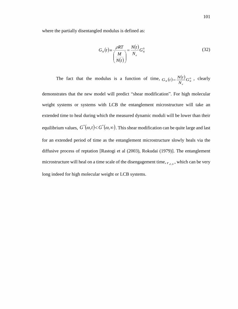
101

where the partially disentangled modulus is defined as:

0

N

e

N GN

tN

tN

M

RTtG

(32)

The fact that the modulus is a function of time, 0

N

e

N GN

tNtG , clearly

demonstrates that the new model will predict “shear modification”. For high molecular

weight systems or systems with LCB the entanglement microstructure will take an

extended time to heal during which the measured dynamic moduli will be lower than their

equilibrium values, ,, ** GtG . This shear modification can be quite large and last

for an extended period of time as the entanglement microstructure slowly heals via the

diffusive process of reptation [Rastogi et al (2003), Rokudai (1979)]. The entanglement

microstructure will heal on a time scale of the disengagement time,0,d , which can be very

long indeed for high molecular weight or LCB systems.

102

VI. SIMULATION OF MONODISPERSE LINEAR PS MELTS AND

ENTANGLED SEMIDILUTE SOLUTIONS IN STEADY AND TRANSIENT

UNIAXIAL EXTENSION

In this Section we explore the properties of the new MBP entanglement dynamics

model for monodisperse systems by numerically solving the system of equations (21) - (32)

summarized in Sec. V. Although the equation set appears complex and formidable they are

all ordinary differential equations that can be stepped forward in time using the simple

Euler method. Because the Euler method is first order in time care must be taken to take

small enough time step sizes to ensure convergence. Using the Euler method makes the

code simple to write and fast to execute. Computational speed becomes an issue when

polydispersity is introduced particularly so when the integral form of the orientation

evolution equation is used [Mishler and Mead (2013a), (2013b)].

We will execute our study by including/excluding various physical effects to isolate

their significance. The physics we are interested in understanding are CCR, ED (through

), and CDFC. The simulation software allows us to turn the specific physics “on”/“off”

and to thereby quantify the impact of the specific physics on rheology. We shall be

particularly interested in the following basic models summarized in Table I. The

experimental data sets, which are used to compare with the calculated prediction results,

are summarized in Table II.

The first simulations we perform are for the flow curves for steady uniaxial

extension of monodisperse PS melts. For these simulations we shall choose a value of

12.0 (ED “on”) in equation (27). This value is chosen such that the shear stress – shear

rate curve is monotonic (see Fig. 10 of Section VIA).

103

A monotonic shear stress – shear rate curve is necessary for stable shear flow

[Ianniruberto and Marrucci (2001)]. All values of 12.0 yield monotonic shear stress –

shear rate curves. The first system we shall study is PS200K (130 oC monodisperse PS melt

by Bach et al.’s (2003)) in steady state extensional flow. The average equilibrium number

of entanglements per chain in this system is 15. The results of a variety of simulations are

shown in Fig. 3 along with the experimental data. The base case for comparison is the

DEMG model which has no ED, CCR or CDFC. The DEMG line in Fig. 3 shows a ladle

shaped flow curve. The upturn in viscosity is associated with the onset of chain stretching

and occurs when the stretch Weissenberg number is about unity, 1, eqs . Complimentary

to the DEMG model is the MLD “toy” model which is simply the DEMG model with CCR

switched “on”. Here again we see the ladle shaped flow curve, lowered relative to the

DEMG model by the additional relaxation mechanism of CCR. The predicted flow curves

of both the DEMG and MLD models are qualitatively and quantitatively at odds with the

experimental data.

The next simulation we execute is the base DEMG model with CDFC now turned

“on” (DEMG-cdfc). Its flow curve is now monotonic extension thinning and closely

mimics the experimental data both before and aftereqs,

1

. This result, and those presented

in what follows, strongly suggest that CDFC is the essential feature needed to achieve a

monotonic thinning extensional flow curve for monodisperse PS melts [Desai and Larson

(2014)].

104

The simulation results are sensitive to the details of the specific expression for

CDFC used. In particular, the details of the form of the expression forKuhnS used matter in

the simulations. The shape of the flow curve is determined by the specific functional form

of CDFC used (see equations (24-26)). In particular, to achieve a monotonic flow curve

CDFC must be activated slightly beforeeqs,

1

. If CDFC is activated later than

eqs,

1

, a

“kink” will occur in the flow curve. Precisely when CDFC is activated depends on the

specific functional form of the CDFC we use.

The next simulation we perform is to include ED in the simulation. In this case, we

choose 12.0 with both CCR “on” and CDFC “on”, i.e. the MBP model. ED is “on” for

any 01 . This generates the black solid curve in Fig. 3. Here for eqs ,

1

, we observe

excessive thinning with lower viscosity values relative to those for DEMG-cdfc which is

caused by CCR. The curve also shows an upturn around eqs,

1

due to the onset of stretch.

However, for eqs ,

1

, it becomes a thinning curve again, approximately parallel to the

DEMG-cdfc case. This thinning effect is due to the effects of CDFC being activated.

Hence, the results especially at eqs ,

1

are approximately equivalent to the DEMG-cdfc

model when we add ED despite the fact that the internal workings of the two models are

entirely different. In particular the average number of entanglements is dramatically lower

when ED is turned “on” resulting in a lower modulus. The lower modulus implies a

105

different entanglement microstructure relative to the DEMG model with CDFC now turned

“on” which predicts a constant entanglement density.

The final simulation we perform is with 12.0 , ED “on”, CCR “off” and CDFC

“on” (MBP-xccr). This is shown as the blue dashed line curve in Fig. 3. As with the DEMG-

cdfc model, the MBP-xccr model generates results very close to the experimental data. The

flow curve shows a much smaller “kink” right after eqs,

1

than that of the MBP curve

and closely mimics the experimental data. The small “kink” is the result of stretch being

activated prior to CDFC being activated. Choosing a different functional form for CDFC

can in principle eliminate this “kink” by modifying precisely when CDFC is activated

relative to eqs,

1

. Precisely when CDFC is activated is impacted by whether ED and CCR

are “on” or “off”. The details of the models, including when CDFC is activated, are

displayed in the Fig.s of Appendix C.

We now address the perplexing question of why the simulations of the “straight”

DEMG-cdfc are very similar to the new MBP-xccr model with 12.0 , i.e. although the

details of the two models, such as the number of entanglements and the modulus, are

profoundly different, they nevertheless yield approximately equivalent extensional flow

curves in close agreement with experimental data. Fig. 4 plots the average number of

entanglements per chain versus extension rate for 12.0 with CCR “off” and CDFC “on”

(MBP-xccr model). We see that for fast extensional flows the average number of

entanglements per chain is approximately half that at equilibrium. Physically, the modulus

is the manifestation of the entanglement microstructure (see equation (32)) and hence the

106

modulus drops off proportionately. Thus, the new MBP-xccr model predicts significant

changes in the entanglement microstructure in fast extensional flow.

Figure 5 plots the steady state relative stretches, and Λ, for the two different

models (DEMG-cdfc and MBP-xccr) versus extension rate. Clearly the relative stretch of

the MBP simulations, Λ, is significantly larger than the relative stretch of the DEMG-cdfc

simulation, . The reason that these two simulations yield approximately equivalent

extensional flow curves is that the effect of ED on the modulus, equation (32), is effectively

canceled by the corresponding increase in stretch. Using the expression for the stress (31)

we argue that for the two models the following products are proportional to the extensional

stress and are approximately equal even though :

tGttG DEMGcdfcNMBPxccrN

202 (33)

Here we have made the assumption that orientation has effectively saturated when

stretch commences. The saturated orientation cancels on both sides of (33). We have also

assumed that the non-Gaussian factors sk are both close to unity and cancel. Note that for

any given model with ED the following equality holds;

tGtN

Nt

N

tNGttG EDN

e

ED

e

NEDN

20202

(34)

Here, tED

2 represents the stretch relative to the equilibrium extension in any

model with ED. Hence, another way to see the approximation in (33) is to note that both

the DEMG-cdfc and MBPxccr models yield similar expressions for the extensional stress

107

in fast steady extension, (34). However, note that tED

2 and tDEMG

2 are calculated

differently in each model and hence are not equal.

The argument underlying equation (33) may very well explain the apparent

“success” of the mono and polydisperse MLD models in predicting nonlinear flows despite

the fact that all MLD models assume a constant entanglement density [Mead (1998), Mead

(2011a), Mishler and Mead (2013a,b)].

In Fig. 6 we examine the transient extensional viscosity versus time for the PS200K

melt. Transient extensional viscosities are more typical of what one encounters in practice

since steady state (Hencky strains greater than ~3) extensional viscosities are very difficult

to achieve experimentally. The specific case that we examine is for an extension rate of

0.01 sec-1 which corresponds to a stretch Weissenberg number of 1, eqs . Note the broad

maximum in the MBP curve at a Hencky strain of ~1.5. The cause of the maximum is that

entanglement dynamics [ tN ] is controlled by ED and lags the stress, only slowly

approaching its steady state value. As in the case for the steady uniaxial flow curves, the

DEMG-cdfc and MBP-xccr models provide the best fit to the data.

The next transient extensional experiment we examine is stress relaxation after

imposing 3 Hencky strain units on a PS145K at 120oC. These experiments were performed

by Yaoita et al. (2012) and provide definitive, hard experimental evidence for the existence

of CDFC. Fig. 7 displays the results of our simulations along with the experimental data.

Fig. 7 experimentally demonstrates that CDFC accelerates the relaxation following

cessation of stretch. The higher the initial stress, the higher the net Kuhn bond orientation

and the larger the CDFC effect and hence the faster the initial relaxation rate. The

108

systematic increase in the initial rate of relaxation strongly supports the existence of CDFC

and this effect is quantitatively captured in the MBP model. Additionally, for the MBP

model, the entanglement density relaxes on a time scale of sec7800d , much slower than

the time scale shown in Fig. 7. Hence the modulus is lowered relative to the equilibrium

state and persists even though the deformation has ceased and this effect does not impact

the relaxation processes in Fig. 7. This phenomenon is “shear modification”.

Finally, we examine another PS melt, PS545k studied by Huang et al. (2013). The

principal difference between this set of experiments/simulations and Fig. 3 is that the

average number of entanglements per chain is very large, Z~41. Hence the separation

between the equilibrium stretch and orientational relaxation times is correspondingly large

since sd Z 3 . However, despite this distinction the salient features of Fig. 8 are largely

similar to those discussed for the PS200K melt in Fig. 3. In particular, we see an enhanced

sensitivity as to precisely when CDFC is activated relative to the onset of stretch. This

sensitivity manifests itself in the size of the “kink” in the flow curve as discussed above

with respect to Fig. 3. These simulations provide a severe test for the precise functional

form of CDFC used.

Figure 9 shows the steady state experimental extensional flow curves for 20 wt.%

1.95M PS solution at 21oC showing monotonic thinning before, and hardening after,

1, eqs [Acharya et al. (2008)]. The new MBP model qualitatively captures the salient

ladle shape features of the flow curve data as does the straight DEMG model without ED,

CDFC or CCR. Once again, the DEMG-cdfc and MBP-xccr provide the best fits to the

experimental data.

109

Thus the new MBP-xccr model, which includes ED and CDFC, captures both the

monotonic thinning behavior of monodisperse PS melts and the thinning/hardening

behavior observed for entangled PS solutions. For solutions, CDFC is effectively diluted

out and is ineffective due to the factor of p in (13) a point which is also discussed by

Yaoita et al. (2012). Hence, the results from the DEMG and DEMG-cdfc models are almost

identical since CDFC is diluted out and is essentially inactive in semi-dilute solutions.

A. Simulation of monodisperse linear PS melts and solutions in steady and transient

shear flow

Since we are interested in a generally applicable “toy” molecular model, we

examine the predictions of the new MBP model in steady and transient shear flow. Here

the orientations will be lower than in fast extensional flows and we anticipate that CCR

will be more important than it is in fast extensional flows.

The first issue we address is determining the range of allowable values for . We

do this by demanding that the shear stress vs. shear rate curve be monotonic such that,

consistent with most experiments, shear flow of melts is stable [McLeish & Ball (1986)].

Fig. 10 displays the derivative of several shear stress vs. shear rate curves for different

values of . It is evident that the shear stress-shear rate curves are monotonic (all positive

slopes) for all 12.0 and exhibit a broad maximum for 12.0 . Hence for our simulations

we choose the maximum allowable value for 12.0 .

In Fig. 11. we compare the calculated shear flow curve for a 7 wt. % 8.42M PS

solution with experimental data [Pattamaprom and Larson (2001)]. We also compare the

first normal stress difference with data in Fig. 12. In both cases all the models

110

approximately mimic the data. The MBP model improves the agreement with the

experimental viscosity at high shear rates whereas the normal stress differences are under

predicted. Note that the results from the DEMG and DEMG-cdfc models were very similar,

which indicates the effect of CDFC is very weak for solutions as was the case in the

extensional flows of semi-dilute solutions. The flow curve of MBP-xccr in Fig. 12 is very

similar to those of DEMG models but the discrepancy from the experimental data is a little

lower than that of DEMG models.

Figure 13 shows the simulation results of transient shear viscosity of a PS200K-S

melt [Schweizer et al (2004)]. All the models display similar trends to those found in steady

shear flow of solutions with the DEMG-cdfc and MBP-xccr models performing best. The

shear stress overshoot is missed by all models in fast shear flows, = 30 sec-1. This is caused

by the differential form of the orientation evolution equation used in this work rather than

the rigorous integral formulation [Larson (1984), Marrucci (1984)]. Using the original Doi-

Edwards integral evolution equation employing the universal orientation tensor will

significantly improve these fast transient shear simulations at the expense of more complex

simulation software.

111

VII. DISCUSSION/SUMMARY

We have constructed a mathematically and computationally simple “toy” molecular

model that includes ED, CDFC and CCR into the base DEMG “toy” model: the MBP

model. This model is a natural next step in the systematic progression of increasingly

detailed and complex molecular models for entangled linear flexible polymers. This point

can be seen by noting that there are three essential components to the constitutive equation

for a monodisperse polymer melt or an entangled semi-dilute solution. This can be seen by

referencing the stress calculator equation (31). (Note that equations (31) or (35) can be

generated directly from the stress-optical rule which is valid in both the linear and

nonlinear flow regions [Larson (1988)].)

dynamicsnOrientatio

tube

dynamicsStretch

dynamicsnglementEnta

N tSttGt 23 (35)

The three fundamental components of any monodisperse constitutive relationship are; 1)

A quantitative description of the orientation dynamics (21), 2) A quantitative description

of the stretch dynamics (28) and 3) A quantitative description of the entanglement

dynamics (27) (which are manifested in (35) through the nonlinear modulus tGN eq.

(32)). The three essential constitutive equation components are, of course, all coupled and

nonlinear. They also incorporate effects like CDFC in the time scales in their descriptions.

The original Doi-Edwards model assumed no stretch and no entanglement

dynamics only considering the orientation dynamics in (35) [Doi-Edwards (1986)].

Consequently, the original family of Doi-Edwards tube and reptation models is restricted

112

to the linear viscoelastic region. To access more general, nonlinear flow situations, the Doi-

Edwards model evolved naturally and systematically by next including the stretch

dynamics to generate the DEMG model [Pearson et al (1991), Mead et al (1995), Mead

and Leal (1995)]. The next step in the evolutionary progression was the MLD model which

considered entanglement dynamics in the form of constraint release (CCR) in the restricted

context of a constant net entanglement density [Mead et al (1998)]. The new MBP model

relaxes the final restriction of a constant entanglement density in order to access nonlinear

flow phenomena far from equilibrium. In the above manner we can see the logical and

systematic progression/evolution of molecular models starting from the seminal work of

de Gennes and Doi-Edwards.

The new MBP model generates extensional flow curves that are monotonic thinning

(with a small “kink” near 1, eqs ) for monodisperse PS melts qualitatively consistent

with experiment. The results are sensitive to the specific functional form of CDFC used

and the predictions could potentially be improved by modifying the expression for CDFC

to fit the flow curve data (equations 24-26). We have not performed this exercise but could

do so in principle. We have used a shifted version of the specific functional form of CDFC

calculated by Ianniruberto et al. (2012) which has a sound theoretical basis underlying it.

For monodisperse PS solutions the effects of CDFC are effectively diluted out and the

classical tube model ladle shaped extensional flow curve is generated. The simulation

results strongly suggest that CDFC is important in the prediction of rheological properties

in nonlinear extensional flows of monodisperse PS melts. CCR is detrimental to the

predictions in extensional flows but is important for the rheological properties in shear

flows.

113

We have also provided a plausible explanation as to why the DEMG-cdfc model

yields a monotonic thinning flow curve of monodisperse PS melts that are approximately

equivalent to those predicted by the new MBP-xccr model, i.e. DEMG with ED “on”,

CDFC “on” and CCR “off”. This may partially explain the previous apparent “success” of

the mono and polydisperse MLD models in predicting phenomena such as the Cox-Merz

rule even though the flow curves calculated assume a constant entanglement density [Mead

(2011b)]. This suspicious coincidence masks the underlying details that are actually

occurring in fast nonlinear flows of entangled polymers. Our new model simultaneously

captures nonlinear flows and the entanglement microstructure modification that occurs in

these fast flows.

Incorporating ED into the model allows the nonlinear phenomenon of “shear

modification” to be captured by the model [Dealy and Wissbrun (1989)]. Shear

modification manifests itself in linear polymer melts with broad, high MWD and melts

with LCB. Direct measurement of the reduced modulus during or after shear or extension

would provide an excellent test of the new ED model [Mead (2013)]. Note that current

molecular constitutive models for polymer systems with LCB do not predict “shear

modification” despite the fact that this is a prominent nonlinear property [McLeish and

Larson (1998)].

Generalizing the new MBP model to polydisperse systems is straightforward and

is performed in Appendix B. Having a generally applicable model for polydisperse systems

that is easy to code and fast to execute has many practical applications in analytic rheology.

114

We shall pursue applications such as MWD determination from transient extensional

rheology experiments in future work.

Finally, knowledge of the melt entanglement density following polymer shaping

operations (finite deformations) is crucially important with respect to determining the

ultimate mechanical properties of the part. Specifically, crystallization processes are

severely impacted by the entanglement density of the melt [Yamazaki et al. (2006), Wang

et al. (2009), Eder et al. (1990)]. The morphology of the resulting crystallites determines

the physical and mechanical properties of the final product [Rastogi et al. (2003)]. Hence,

the information gleaned from molecular models with ED, such as the MBP model, is

directly relevant to polymer processing operations.

115

FIG. 1. Schematic diagram for tube shortening when 1

tubeS : The tube is crinkled and

constraint release shortens the tube and relaxes stretch and orientation [Mead et al. (1998),

Mead (2011a)].

FIG. 2. Schematic diagram for tube shortening when 1tube

S : Constraint release does not

relax any stretch. Note that the tube is unraveled and linear rather than in a zig-zag cat’s

cradle (back folded) conformation ( 1tube

S in both cases). Fast, large deformations

unravel the chain and generate highly extended nearly linear conformations [Desai and

Larson (2014) see Fig. 1].

116

FIG. 3. Steady state extensional viscosity as a function of extension rate: Experimental

data is for monodisperse PS200K at 130oC [Bach et al. (2003)]. Predictions are from

various options of the family of models (see Fig. legend and Table 1). This allows us to

determine that CDFC is the essential ingredient required to capture the monotonic

extensional flow curve of monodisperse PS melts. The “kink” in the MBP flow curve

begins at 1, eqs .

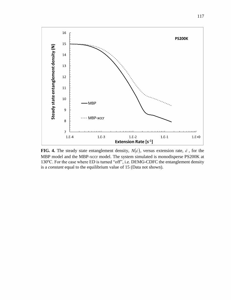
117

FIG. 4. The steady state entanglement density, N , versus extension rate, , for the

MBP model and the MBP-xccr model. The system simulated is monodisperse PS200K at

130oC. For the case where ED is turned “off”, i.e. DEMG-CDFC the entanglement density

is a constant equal to the equilibrium value of 15 (Data not shown).

118

FIG. 5. The relative stretches for MBP, MBP-xccr, and DEMG-cdfc. The respective curves

are: vs. (DEMG-cdfc) and vs. (MBP and MBP-xccr) for the monodisperse

PS200K melt. The relative stretch is increased relative to the base DEMG-cdfc case

by virtue of the unraveling of back folds that occurs in the new model [Desai and Larson

(2014)].

119

FIG. 6. Transient extensional viscosity, te versus t , for monodisperse PS200K at an

extension rate of 0.01 sec-1 ( 1, eqs ). Note the small and broad maximum in the transient

viscosity at a Hencky strain of ~1.5 for the MBP model. This is caused because ED lags

the stress, i.e. it takes many Hencky strain units to partially disentangle the melt. Note that

the results from the DEMG and DEMG-cdfc models are effectively on top of each other

since this extension rate is below the onset of CDFC threshold.

120

FIG. 7. Normalized stress relaxation after imposing 3 Hencky strain units for a

monodisperse PS145K melt at 120oC at three different steady extension rates. The higher

the extension rate, the higher the net Kuhn bond orientation and the greater the effect of

CDFC on the initial rate of stress relaxation. The MBP model captures this effect.

121

FIG. 8. Steady state extensional viscosity as a function of extension rate. Experimental

data is for monodisperse PS545K melt at 130oC [Huang et al. (2013)]. Predictions are from

various options of the family of models (see Fig. legend and Table 1). Once again the

DEMG-CDFC and MBPxccr models perform best.

122

FIG. 9. Steady state extensional viscosity as a function of extension rate. Experimental

data is for a monodisperse 20% 1.95M PS solutions at 21oC [Acharya et al. (2008)].

Predictions are from various options of the family of models (see Fig. legend and Table 1).

Note that the results from DEMG and DEMG-cdfc are on top of each other.

123

FIG. 10. The (slope of shear stress-shear rate curve) derivative of steady shear stress with

respect to ,

d

d xy versus for a family of values. For stable shear flow the shear

stress vs shear rate curve must be monotonic (positive slope everywhere). The maximum

value of that yields a monotonic curve of stress-shear rate is 12.0 . The results from

13.0 showed negative values around shear rate of 0.01s-1 (curve not shown).

124

FIG. 11. The shear flow curve, vs. , for a monodisperse PS solution 7% 8.42M PS.

Predictions are from various options of the family of models (see Fig. legend and Table 1).

Note that the results from the DEMG and DEMG-cdfc models effectively superpose since

CDFC is diluted out of this semi-dilute system.

125

FIG. 12. The first normal stress difference for a monodisperse PS solution 7% 8.42M PS

is shown, 1N vs. . Predictions are from various options of the family of models (see Fig.

legend and Table 1). Note that the results from the DEMG and DEMG-cdfc models are on

top of each other since CDFC is diluted out of this system.

126

FIG. 13. Transient monodisperse 200K-S PS melt at shear rates of 1s-1, 10s-1 and 30s-1.

Since the net Kuhn bond orientation is low the effect of CDFC is negligible and the DEMG-

cdfc model is approximately equal to the DEMG model. The poor agreement with data at

30 sec-1 is due to the use of the differential form of the orientation evolution equation.

127

TABLE I: Summary of the family of toy molecular models studied.

Model CCR ED CDFC

DEMG off off ( 0 ) Off

DEMG-cdfc off off ( 0 ) On

MLD on off ( 0 ) Off

MBP on on( 0 ) On

MBP-xccr off on( 0 ) On

TABLE II: Experimental data sets compared (Input parameter estimations were referred

to Desai and Larson (2014) and Likhtman and McLeish (2002). Me=13333 Da is used for

all PS melts to give max=4.2 whereas Me for solutions are evaluated by dividing by p1.2.

The values of τd,f given below include the effect of double reptation.)

Sample

GN0

(kPa)

d,f (s) S,eq (s) Neq Ref

PS200K 200 1610 94.3 15 Bach et al. (2003)

PS200K-S 200 1.33 0.065 15 Schweizer et al. (2004)

PS545K 250 54418 779 41 Huang et al. (2013)

PS145K 290 7839 1134 10.7 Yaoita et al. (2012)

20% 1.95M PS 6.8 6.26 0.17 30.4 Acharya et al. (2008)

7% 8.42M PS 0.52 31.65 0.6 44.3 Pattamaprom & Larson (2001)

128

ACKNOWLEDGMENTS

The authors acknowledge Dr. Morton M. Denn’s helpful comments and use of the

computational facilities at the City College of New York. Partial financial support from the

Materials Research Center and the Energy Research & Development Center of Missouri

University of Science & Technology is also gratefully acknowledged.

129

APPENDIX A: DERIVATION

In this Appendix we derive equation (5) in the main text, the relationship between

the non-equilibrium tube disengagement time Nd

1 , the number of entanglements N and

the equilibrium terminal disengagement time, 0,d . We start with the relationship between

the tube length b and the Kuhn bond length a [Doi and Edwards (1986)]:

22 aMNb k (A1)

Here, N is the number of entanglements (tube segments). The end-to-end distance of the

tube segments and Kuhn bonds within them must be equal. kM is the number of Kuhn

segments of length a . Hence, the tube length b is related to the number of entanglements

through:

a

N

Mb k

2

1

2

1

(A2)

The equilibrium tube contour length, NbLeq , is a function of the number of

entanglements N,

aMNNbL keq

2

12

1

(A3)

Note that eqL is a monotonically increasing function of N.

130

The terminal tube disengagement time d is related to the tube length through [Doi

and Edwards (1986)],

c

eq

dD

L

2

2

(A4)

Here o

cM

kTD

is the curvilinear diffusion coefficient and o is the monomeric friction

coefficient. We define the equilibrium terminal disengagement time as

c

ke

c

eq

dD

bMN

D

L

2

2

2

2

0,

where eN is the equilibrium number of entanglements.

Substituting these expressions into equation (A1.4) above yields the result (5):

0,

1

d

e

dN

NN

(A5)

131

APPENDIX B: GENERALIZATION OF THE NEW EDS – CDFC MLD TOY

MODEL TO POLYDISPERSE SYSTEMS

In this Appendix we outline the manner in which the ideas presented in the main

text can be generalized to describe polydisperse systems. In this Section i-j subscripts

denote components of the MWD and not tensor components [Mead (2007)].

The ij entanglement pair dynamics are described by the following equation which

generalizes eq. (1):

diffusiontipmatrixj

jd

ijij

ntsentanglemeijofndestructioconvective

ij

i

i

i

i

tubei

diffusiontipchaini

id

ijij

ijt

tNNtN

ttS

t

tNNtN

1

,

0

,1

,

0

:

(B1)

Here, tN ij represents the number of j entanglements on an i chain and

e

i

jiejijM

MwNwN ,

0

represents the equilibrium number of j entanglements on an i-chain

and e

i

ieM

MN ,

is the total equilibrium number of net entanglements on an i chain. ieN , is

a function of molecular weight and the molecular weight between entanglements which is

assumed not to be affected by polydispersity.

The reptation time of an i-chain is modified by the number of current entanglements of all

other chains on the i-chain (eq. 5 and Appendix I),

tN

tN

tN

tNt id

ie

j

ij

id

ie

i

id ,

,

,

,

1

,

(B2)

Of course, CDFC as described in Section IIA will also be present which will reduce tid ,

in fast flows.

132

The first approximation to try for the functional form of the reduced friction CDFC is that

used in our first paper [Park et al. (2012)]:

norientatiobondKuhnmatrixnet

jjKuhnj

norientatiobondKuhn

chaintest

iKuhnid

id

is

is

eq

SwSkttt

,,0

,

,

0

,

,:1

(B3)

The above expression is written for a polydisperse system where the components

are denoted by subscripts and jw represents the weight fraction of MW component j. The

effect of Kuhn bond concentration is accounted for in the weight fraction of matrix

polymers and/or solvent. The relative orientation of the test chain and the matrix is

quantified by the double dot product of the two orientations.

This is one possible algorithm that we propose for CDFC of the polydisperse MLD model.

Other functional forms for the dependence of the friction factor on relative test chain –

matrix Kuhn bond alignment can be tried too. For example by generalizing (24) we see

that:

65.1

,

2

,

2

65.1

,,,,0

,

,

0

,

,

:02239.0

:02239.0:

jjtubejjitubei

jjKuhnjiKuhn

jjKuhnjiKuhn

id

id

is

is

eq

SxwSx

SwSSwSftt

(B4)

This function approximates the monodisperse case, equation (24). Note that for

most common commercial molecular weight distributions the effects of CDFC will largely

disappear due to the lower overall level of Kuhn bond orientation in polydisperse systems

under ordinary flow conditions. The low MW components effectively act as solvent for the

high MW components [Mead (2011b)].

133

The i-component partially disentangled chain stretch equation remains unchanged:

shorteningtubeCCR

iitube

retractionchain

is

i

is

stretchaffine

ii


i

i

i

i St

tkStt

tt

11

2

11:

,,

,

(B5)

where is the fractional rate of matrix entanglement renewal,

jdjj

j

j

j

jtubej

j

ttSw

,

2,

1:

and itubeS

, is the magnitude of the i-

chain tube orientation,

jijtubejitube

SwS,,

. The nonlinear spring factor tk is , is defined

by (30) for each i chain.

The maximum stretch ratio factor

max

max,

tt

i

i

needs to be calculated to solve

the stretch equation. The easiest way to accomplish this is using the definition of ti

along with the known entanglement pair dynamics, tN ij ,

2

1

,

max

max,

j

ij

iei

itN

Ntt

(B6)

The factor ti in (B6) can be calculated numerically at each time step rather than solving

the ordinary differential equation for ti .

Similarly, the orientation of the ij entanglement pairs obeys the following differential

equation [Mead (2007)]:

03

11:2ˆ

,,

,,,

ijtubeijd

Kuhn

ijtubeijtubeijtubeS

t

SStSttS

(B7)

134

Where the ij entanglement disengagement time ijd , is:

tt

ttS

tttjdjj

j

j

j

jtubeiidiijd ,

2,,

2

,

1:

111

(B8)

And KuhnS is the net matrix Kuhn bond orientation,

itubei

i

iiKuhn

i

iKuhn SxwSwS,

2

,

.

Of course, the Kuhn bond conformation dependence (CDFC) of the disengagement and

stretch times is applicable. This is why we write both tid ,

and tis ,

as functions of time.

Additionally, the effect of “solvent like” entanglements with respect to stretch processes

needs to be accounted for in polydisperse systems. This can be accomplished in the manner

described in Mishler and Mead (2013a,b) where entanglements with an average lifetime

less than the Rouse time act as solvent with respect to stretch relaxation processes.

The expression for the stress is more involved and requires some discussion. Consider the

expression for the stress from the polydisperse MLD model without entanglement

dynamics:

i

S

jijtubejiis

uluschaini

Niitubeiis

i

Ni

itube

tSwkGwSkGwt

,

,

2

,

mod

0

,

2

,

0 33

(B9)

Here e

NM

RTG

0

represents the equilibrium value of the modulus and eM is the molecular

weight between entanglements which for the MLD model is a constant. The factor isk ,

represents the effects of the i-component finitely extensible nonlinear spring, eq. (30). In

(A2.9) we have assumed that

i e

i

i

iNNM

RTGG

,

. However ii w

so that

0

, Ni

e

iiN GwM

RTwG

, hence (A2.9).

135

We need to generalize this expression to allow for varying degrees of deformation

induced disentanglement where the molecular weight between entanglements varies from

component to component in the MWD. The non-equilibrium modulus can be written as

tM

RTG

ie

i

iN

,

,

. Here, tM ie, is the molecular weight between entanglements on the i-

component. In the polydisperse case with varying degrees of disentanglement two things

in the expression for NG change: ii w

the number of i-strands per unit volume and the

molecular weight between entanglements on i-component chains

tN

MtM

i

i

e

.

With these two changes in mind we can write the non-equilibrium i-chain modulus

iNG , by analogy to the monodisperse equilibrium case.

moduluschaini

ie

k

ik

NiN

ie

i

i

ie

i

N

tN

GwGN

tNw

tM

RT

,

00

,,

(B10)

So, using the above expression for the i-chain modulus we can write the stress for a system

with arbitrary polydispersity as:

i

S

jijtubejiis

moduluschaini

N

ie

k

ik

i

itube

tSwttkGN

tN

wt

,

,

2

,

0

,

3

(B11)

As with the monodisperse case, polydisperse systems are predicted to display shear

modification since tN ik will recover its equilibrium entanglement density ieN , on

reptation time scales which can be extremely long for high molecular weight entanglement

pairs.

136

We anticipate that for typical commercial polydisperse polymer melts most of the

effects of CDFC discussed in this paper will disappear since the average level of Kuhn

bond orientation will be low. However, this will not be the case for the entanglement

dynamics effects. The effects of ED such as “shear modification” will manifest themselves

for broad polydisperse melts with high molecular weight tails [Dealy and Tsang (1981),

Rokudai (1979)].

137

APPENDIX C: INTERNAL DETAILS OF THE MODEL CALCULATIONS

In this Appendix we detail the inner model workings underlying Fig. 3. In this way

the mechanisms responsible for the observed uniaxial flow curves can be readily

understood. In Fig. 14 the steady state orientation as a function of extension rate is

displayed for the system described in Fig. 3. Similarly, Fig. 15 displays the steady state

Kuhn bond orientation as a function of extension rate. An inflection point is seen in the

curves at 1, eqs corresponding to the onset of significant stretch. CDFC effects set in for

Kuhn bond orientations greater than 0.1. Finally, Fig. 16 displays CDFC, 0

,

,

is

is

eq

, as a

function of extension rate and the onset of CDFC effects is clearly shown. All of the above

Fig.s can be correlated to the extensional viscosity flow curve shown in Fig. 3 and obvious

conclusions concerning the causes for the various features can be drawn. In particular,

precisely when CDFC is activated relative to eqs,

1

is impacted by whether ED and CCR

are “on” or “off”. Choosing a different functional form for CDFC can in principle modify

precisely when CDFC is activated relative to eqs,

1

.

138

FIG. 14. Steady state orientation as a function of extension rate for monodisperse PS200K

at 130oC [Bach et al. (2003)]. Predictions are from various options of the family of models

(see Fig. legend and Table 1). This allows us to determine the orientation levels when

stretch and CDFC commence. The equilibrium stretch relaxation time is 94, eqs sec

which doesn’t include the effects of CDFC.

139

FIG. 15. Steady state Kuhn bond orientation as a function of extension rate for

monodisperse PS200K at 130oC. Predictions are from various options of the family of

models (see Fig. legend and Table 1). The equilibrium stretch relaxation time is 94, eqs

which doesn’t include the effects of CDFC. CDFC commences when Kuhn bond

orientation is greater than 0.10.

140

FIG. 16. Steady state ratio of 0

,

,

is

is

eq

as a function of extension rate for monodisperse

PS200K at 130oC. The equilibrium stretch relaxation time is 94, eqs sec which doesn’t

include the effects of CDFC. Predictions are from various options of the family of models

(see Fig. legend and Table 1).

141

References

Acharya, M. V., P.K. Bhattacharjee, D.A. Nguyen and T. Sridhar, “Are Entangled

Polymeric Solutions Different from Melts?” AIP Conf. Proc. 1027, 391-393 (2008).

Andreev, M., R.N. Khaliullin, R.J.A. Steenbakkers and J.D. Schieber, “Approximations of

the discrete slip-link model and their effect on nonlinear rheology predictions”, J.

Rheol. 57, 535-557 (2013).

Bach, A., K. Almal, O. Hassager and H.K. Rasmussen, “Elongational viscosity of narrow

molar mass distribution polystyrene”, Macromolecules 36, 5174-5179 (2003).

Baig, C., V.G. Mavrantzas and M. Kroger, “Flow effects on melt structure and

entanglement network of linear polymers: Results from a non-equilibrium molecular

dynamics study of a polyethylene melt in steady shear”, Macromolecules 43, 6886-

6906 (2010).

Bhattacharjee, P.K., J.P. Oberhauser, G.H. McKinley, L.G. Leal and T. Sridhar,

“Extensional rheometry of entangled solutions”, Macromolecules 35, 10131-10148

(2002).

Cohen, A., “A Padé approximant to the inverse Langevin function”, Rheol. Acta 30, 270-

273 (1991).

Dealy, J.M. and WM. K.-W. Tsang, “Structural time dependency in the rheological

behavior of molten polymers”, J. Appl. Poly. Sci. 26, 1149-1158 (1981).

Dealy, J.M. and K.F. Wissbrun, Melt Rheology and its Role in Plastics Processing Van

Norstrand Reinhold (1989).

Desai, P.S. and R.G. Larson, “Constitutive model that shows extension thickening for

entangled solutions and extension thinning for melts”, J. Rheol. 58, 255-279 (2014).

Doi, M., and S.F. Edwards, The Theory of Polymer Dynamics, Oxford Science Publications,

(1986).

142

Doi, M., D.S. Pearson, J. Kornfield and G.G. Fuller, “Effect of nematic interaction in the

orientational relaxation of polymer melts”, Macromolecules 22, 1488-1490 (1989).

Eder, G., H. Janeschitz-Kriegl, and S. Liedauer, “Crystallization processes in quiescent and

moving polymer melts under heat transfer conditions”, Progress Polymer Sci. 15,

629–714(1990).

Everaers, R., S.K. Sukumaran, G.S. Grest, C. Svaneburg, A. Sivasubramanian and K.

Kremers, “Rheology and microscopic topology of entangled polymeric liquids”,

Science 303, 823-827 (2004).

Flory, P. J., Statistical Mechanics of Chain Molecules Interscience, New York, (1969).

Graham, R.S., A.E. Likhtman, T.C.B. McLeish and S.T. Milner, “Microscopic theory of

linear, entangled polymer chains under rapid deformation including chain stretch and

convective constraint release”, J. Rheol. 47, 1171-1200 (2003).

Huang, Q., O. Mednova, H.K. Rasmussen, N.J. Alvarez, A. L. Skov, K. Almdal, and O.

Hassager, “Concentrated Polymer Solutions are Different from Melts: Role of

Entanglement Molecular Weight”, Macromolecules 46, 5026-5035 (2013)

Ianniruberto, G, A. Brasiello, G. Marrucci, “Friction Coefficient Does Not Stay Constant

in Nonlinear Viscoelasticity”, Proceedings of the 7th Annual European Rheology

Conf., pg. 61, (2011).

Ianniruberto, G., A. Brasiello and G. Marrucci, “Simulation of fast shear flows of PS

oligomers confirm monomeric friction reduction in fast elongational flows of

monodisperse PS melts as indicated by rheooptical data”, Macromolecules 45, 8058-

8066 (2012).

Ianniruberto, G., and G. Marrucci, “On compatibility of the Cox-Merz rule with the model

of Doi and Edwards”, J. Non-Newtonian Fluid Mech. 65, 241–246 (1996).

Ianniruberto, G., and G. Marrucci, “A simple constitutive equation for entangled polymers

with chain stretch”, J. Rheol. 45, 1305-1318 (2001).

143

Ianniruberto, G., and G. Marrucci, “Convective constraint release revisited”, J. Rheol. 58,

89-102 (2014).

Larson, R.G., Constitutive Equations for Polymer Melts and Solutions, Butterworths

(1988).

Larson, R.G., “A constitutive equation for polymer melts based on partially extending

strand convection”, J. Rheology 28, 545-572(1984).

Leblans, P.J.R., and C. Bastiaansen, “Shear modification of low density polyethylene: Its

origin and its effect on the basic rheological functions of the melt”, Macromolecules

22, 3312-3317 (1989).

Likhtman, A. E., and T. C. B. McLeish, ‘‘Quantitative theory for linear dynamics of linear

entangled polymers,’’ Macromolecules 35, 6332–6343 (2002).

Marrucci, G.G., in Advances in Transport Processes Vol. V A.S. Majumdar and R.A.

Mashelkar, Eds. John Wiley & Sons (1984).

McLeish, T.C.B. and R.C. Ball, "A molecular approach to the spurt effect in polymer melt

flow", J. Poly. Sci. Poly. Phys. Ed. 24, 1753-1745 (1986).

McLeish, T.C.B. and R.G. Larson, “Molecular constitutive equations for a class of

branched polymer: the pom-pom polymer”, J. Rheol. 42, 81-110 (1998).

Mead, D.W., D. Yavich and L. Leal, "The reptation model with chain stretching I) Basic

equations and general properties", Rheologica Acta 34, 339-360(1995).

Mead, D.W. and L. Leal, "The reptation model with chain stretching II) Steady flow

properties", Rheologica Acta 34, 360-383(1995).

Mead, D.W., R.G. Larson and M. Doi, “A molecular theory for fast flows of entangled

polymers”, Macromolecules 31, 7895-7914 (1998).

144

Mead, D.W., “Development of the “Binary Interaction” Theory for Entangled Polydisperse

Linear polymers”, Rheol. Acta 46, 369-395 (2007).

Mead, D.W., “Derivation of the “Switch Function” in the Mead-Larson-Doi Theory”,

Rheologica Acta 50, 631-643 (2011a).

Mead, D.W. , “Analytic Derivation of the Cox-Merz Rule Using the MLD “Toy” Model

for Polydisperse Linear Polymers”, Rheol. Acta 50, 837-866 (2011b).

Mead, D.W., “Small Amplitude Oscillatory Shear Flow Superposed on Parallel or

Perpendicular Steady Shear of Polydisperse Linear Polymers: The MLD Model”, J.

Non-Newtonian Fluid Mech. 195, 99-113 (2013).

Mewis, J., and M.M. Denn, “Constitutive equations based on the transient network

concept”, J. Non-Newtonian Fluid Mech. 12, 69-83 (1983).

Mishler, S.D. and D.W. Mead, “Application of the MLD “Toy” Model to Extensional

Flows of Broadly Polydisperse Linear Polymers: Model Development”, J. Non-

Newtonian Fluid Mech. 197, 61-79 (2013a).


Flows of Broadly Polydisperse Linear Polymers: Comparison to Experimental data

Sets”, J. Non-Newtonian Fluid Mech. 197, 80-90 (2013b).

Park, J., D.W. Mead, and M.M. Denn, “Stochastic Simulation of Entangled Polymeric

Liquids in Fast Flows: Microstructure Modification”, J. Rheol. 56, 1057-1082 (2012).

Pattamaprom, C. and R.G. Larson, “Constraint release effects in monodisperse and

bidisperse polystyrenes in fast transient shearing flows”, Macromolecules 34, 5229-

5237 (2001).

Pearson, D. S., E. A. Herbolzhiemer, N. Grizzuti, and G. Marrucci, “Transient behavior of

entangled polymers at high shear rates”, J. Polymer Sci., Part B: Polymer Phys. Ed.

29, 1589-1597 (1991).

145

Rastogi, R., L. Kurelec, J. Cuijpers, D. Lippits, M. Wimmer, P. J. Lemstra, “Disentangled

State in Polymer Melts; A Route to Ultimate Physical and Mechanical Properties”,

Macromolecular Materials Eng. 288, 964–970 (2003).

Rokudai, M., “Influence of shearing history on the rheological properties and

processability of branched polymers”, J. Appl. Poly. Sci. 23, 463-471 (1979).

Schweizer, T., J. van Meerveld, and H. C. Ottinger, “Nonlinear shear rheology of

polystyrene melt with narrow molecular weight distribution—Experiment and

theory,” J. Rheol. 48, 1345–1363 (2004).

Treloar, L.R.G., The Physics of Rubber Elasticity 3rd Edition, Oxford University Press

(1975).

Tzoumanekas, C., and Theodorou, D. N., “Topological Analysis of Linear Polymer Melts:

A Statistical Approach”, Macromolecules 39, 4592-4604 (2006).

Wang, X., R. Liu, M. Wu, Z. Wang, Y. Huang, “Effect of chain disentanglement on melt

crystallization behavior of isotactic polypropylene”, Polymer 50, 5824–5827(2009)

Yamaguchi, M., and M.H. Wagner, “Impact of processing history on rheological properties

for branched polypropylene”, Polymer 47, 3629-3635 (2006).

Yamazaki, S., F. Gu, K. Watanabe, K. Okada, A. Toda, M. Hikosaka, “Two-step formation

of entanglement from disentangled polymer melt detected by using nucleation rate”,

Polymer 47 6422-6428(2006).

Yaoita, T., T. Isaki, Y. Masubuchi, H. Watanabe, G. Ianniruberto and G. Marrucci,

“Primitive chain network simulation of elongational flows of entangled linear chains:

Stretch/orientation induced reduction of monomeric friction”, Macromolecules 45,

2773-2782 (2012).

Yaoita, T., Y. Masubuchi and H. Watanabe, “Concept of stretch/orientation reduction

tested with a simple constitutive equation”, Nihon Reoroji Gakkaishi, 42, 207-213

(2014).

146

III. Constitutive model for polydisperse entangled polymers incorporating

binary entanglement pair dynamics and a configuration dependent friction

coefficient

Synopsis

The concepts of entanglement dynamics (ED) and configuration dependent friction

coefficient (CDFC) in our previous monodisperse Mead-Banerjee-Park (MBP) “toy”

constitutive model [Mead et al., J. Rheol. 59, 335-363 (2015)] have been combined with

that of diluted stretch tube theory of Mishler and Mead [J. Non-Newtonian Fluid Mech.

(2013)] to develop the polydisperse MBP “toy” constitutive model. The model is first used

in the “forward” direction to predict the nonlinear viscoelastic material properties of model

polydisperse systems. The polydisperse MBP toy model accurately predicts the material

properties in the forward direction for transient and steady uniaxial extension and shear

flow melt and solution conditions. The model can correctly generate the long and short

chain component contributions to the rheological property measured.

147

I. INTRODUCTION

In our previous paper we developed the Mead-Banerjee-Park (MBP) “toy”

constitutive model for entangled monodisperse linear flexible polymers that displayed

considerable promise in predicting both extensional and shear flow properties in the highly

nonlinear flow regime [Mead et al (2015)]. In this paper we continue our study of the MBP

model by examining model polydisperse systems in fast extensional and shearing flows.

We shall consider both model and general molecular weight distributions with P discrete

weight fractions, 11

P

j

jw . Here and throughout this paper subscripts denote discrete

molecular weight components not tensor component indices.

As pointed out by Mishler and Mead (2013a and b), construction of a naïve

polydispersity model is straightforward given the monodisperse MBP model developed in

Appendix B of Mead et al., (2015). However, this naïve construction does not take account

of the fact that for systems with broad polydispersity low molecular weight components

may have an orientational relaxation time less than the stretch relaxation time of the high

molecular weight component (See Figure 1).

In this case, the low molecular weight components act effectively as “solvent” with

respect to the stretch processes of the long chains. This fact necessitates the construction

of a “diluted stretch tube” to describe stretching processes for polymer systems with broad

molecular weight distribution (MWD) in nonlinear flows [Mishler and Mead (2013a and

b)].

148

Hence, we incorporated the dilute tube theory into the monodisperse MBP to

develop a new “toy” constitutive model for the improved prediction of viscoelastic material

properties of polydisperse systems. Note here that our new model for polydisperse system

is called as “MBP” model whereas the previous model for monodisperse system is

distinguished as “monodisperse MBP”. The model by Mishler and Mead (2013a and b)

will be abbreviated as “MM” model.

In this paper, as in our previous work [Mead et al., (2015)], we use the term “tube”

despite the fact that we believe that defining entanglements as discrete pair-wise couplings

between two chains is a more accurate physical description of chain-chain interactions.

Indeed, the traditional “tube” is an unhelpful concept in nonlinear rheology. Invoking a

“tube” effectively fixes the entanglement density at a prescribed level consistent with the

“tube diameter”. Thus the tube concept is not conducive to simple descriptions of

entanglement dynamics since this would necessitate a continuously varying dynamic tube

diameter.

We believe that a simpler and more natural approach is to describe the viscoelastic

properties in terms of the pair-wise entanglement dynamics as the conceptual paradigm

rather than a mean field “tube”. Hence, when we use the term “tube” in this paper we mean

a series of discrete, oriented ij entanglement couplings along the test chain.

This paper is organized in the following manner; In Section II we outline how the

dilute tube theory of MM model is combined with the monodisperse MBP model to result

in MBP model. Section III.A uses the MBP model to simulate transient uniaxial extension

for validation against the experimental data and to be compared with the MM model

149

prediction. Similarly, Section III.B predicts the transient shear flows. Section IV discusses

the effect of polydisperse components on the rheological properties. Section V summarizes

and concludes our results.

150

II. THE POLYDISPERSE MBP “TOY” MODEL FOR LINEAR POLYMERS

A. Incorporation of dilute tube theory into the monodisperse MBP model

In this Section we outline the manner in which the entanglement dynamics ideas

proposed by Mead et al., (2015) and Mishler and Mead (2013a, b) can be generalized to

describe polydispersity within the MBP “toy” model framework (See Appendix B of Mead

et al., (2015)). As alluded in the introduction, in the general MWD case we shall have to

consider the possibility that some components of the MWD act like “solvent” with respect

to stretch of the i-component. As we shall see, such situations manifest themselves for

MWD’s with polydispersity indices (PI) greater than around 2. Specifically, solvent-like

entanglements with respect to stretch occur when there is overlap in the stretch and

orientational relaxation spectra (Figure 2).

Generalizing the i-component toy stretch equation for polydisperse systems with

broad MWD’s requires discussion. As proposed in previously published work by Mishler

and Mead, entanglements with a lifetime less than the Rouse (stretch) relaxation time

effectively act as solvent with respect to stretch processes of the test chain. The criteria

1

,

,

jdi

is

t

defines a “cut-off” molecular weight, jM , relative to the test chain

molecular weight, iM , splitting the MWD into solvent-like and full entanglement

151

fractions with respect to stretch relaxation processes of the i-chain†, see Figure 2. Auhl et

al have demonstrated that the effective (experimentally observed) stretch relaxation eff

is,

is altered from the bare Rouse time is, by “stretch tube dilution” such thati

iseffis

,,

. Here,

ti1 is the “dilution” level of solvent like entanglements with respect to stretch of

the long chains defined by the cutoff criteria 1,

,

jdi

is

(see Figure 2);

tN

tN

tN

tN

ti

cutj

ij

j

ij

cutj

ij

i

(1)

Physically, Eq (1) represents the fraction of viable stretch entanglements. Note that

entanglement densities replace weight fractions in the definition of ti . Note that we

have had to generalize the definition of ti

to account for the ij entanglement dynamics

which were not considered in the work of Mishler and Mead (2013).

† In order to calculate

tN

tN

tN

tN

ti

cutj

ij

j

ij

cutj

ij

i

self consistently an iterative procedure is

required. For the first iteration we choose 1i and determine a new dilution level and cut-off molecular

weight. The new value of i is then fed into the cut-off criteria and this iterative process is repeated until

convergence is achieved (Figure 2). This procedure is necessary to generate a dilution level that is self-

consistent with the definition of the effective stretch relaxation time we use in the diluted stretch tube,

i

iseffis

,,

. Note that the position of the j-cut changes with time and must be updated accordingly.

152

Similar modifications have to be made in the definition of tSdi,

, Eq (6) below.

These are essentially elaborate bookkeeping measures; counting ij entanglement pairs on

the chain when entanglement dynamics and stretch tube dilution are operational (see Figure

3. for a qualitative illustration of the model, identification of variables and the hierarchy of

“tubes”).

The main polydispersity ideas and equations are detailed by Mead et al., (2015)

Appendix B. We summarize the MBP model equations previously described by Mead et

al., (2015) and the diluted stretch tube model of Mishler and Mead (2013a) in Section II.B.

As described in Mishler and Mead, the purpose of creating a diluted stretch tube is

to calculate the i-chain stretch in systems with broad MWDs where some of the

entanglements are solvent-like with respect to stretch processes of a given test chain (see

Figure 2). Subsequent work by Mead et al., (2015) revealed that entanglement dynamics

reduce the entanglement density and this effect also needs to be factored into the i-chain

stretch dynamics equation. The result is that we calculate the stretch in the diluted and

partially disentangled stretch “tube” (see Figure 3.). This stretch, tdi, , is then related to

the stretch in the partially disentangled “tube”, ti , through the stretch coupling Eq (9).

Stress is then calculated in the partially disentangled tube, Eq (11). We note that the

expression for the stress, Eq (11), collapses to the correct linear viscoelastic limit after

complete relaxation of the system. In the following section we will take a look at the

equations that have been developed to study the polydisperse systems, both solutions and

melts under shear and extension conditions.

153

B. Summary of the polydisperse MBP “toy” model equations

1) The ij disentangled “tube” entanglement density evolution equation;

t

tNNtN

ttS

t

tNNtN

jd

ijijij

i

i

i

i

tubeiid

ijijij 1

,

0

,1,

0

:

(2)

2) The ij entanglement pair orientation evolution equation;

The orientation tensor tSijtube,

for the slow relaxing stretch entanglements ( cutj )

evolves as;

03

11:2ˆ

,,

,,,

ijtubeijd

Kuhn

ijtubeijtubeijtubeS

t

SStSttS

(3a)

And the orientation tensor tSijtube,

for the fast relaxing ij stretch entanglements

( cutj ) evolves as;

01

:2ˆ,

,,,,

tIS

t

SStSttS

ijijtubeijd

Kuhn

ijtubeijtubeijtube

(3b)

Where the tension induced orientation tensor, tIij

, in the fast relaxing entanglements

( cutj ) is defined as [Mead and Mishler (2013) Eq. (12)]:

3

1331

,1

,

,,

1

,

txL

txtS

txL

txtI

di

di

didi

di

ij

(3c)

154

where

t

ttx

di

di

di

max,

,

,

is the fractional extension of the partially diluted and

disentangled i-tube and the corresponding orientation, tSdi,

, is defined below Eq (6).

3) The i chain diluted and disentangled stretch tube segmental stretch equation;

shorteningtubeCCR

idiitube

retractionchain

is

di

id

glementenviableof

stretchaffine

didi


di

di

di

di St

tkStt

tt

11

2

11: ,,

,

,

,

tan

,,,

,

,

,

(4)

where

2

1

,

,

2

1

,

max,

max,,

tN

N

tN

Ntt

di

ie

cutj

ij

ie

i

didi

(5)

and

t

tStN

tN

tSi

cutjijtube

i

ij

di

,

, (6)

with

t

tt

ttS

ti

cutj jddjdj

dj

dj

dj

dj

i

,

2,,

,

,

,

,

1:

(7)

1/13

/3

3

L

2,

2max,

2,

2max,

2,

2,

2max,

2,

2,

2max,

max,

,

max,

,1

,

diidii

didiididii

id

di

id

di

id

t

t

t

t

tk

(8)

155

4) Diluted and partially disentangled i-stretch tube – partially disentangled i-tube stretch

coupling relationship;

id

diiddii

i

i

i

iiii

i

iii

LxL

xL

L

max,

,1max,,1

max,

1max,

max,

1max,

3

3

31

3

(9)

where i

iix

max,

is the fractional extension of the partially disentangled i-tube.

5) The ij partially disentangled tube entanglement pair relaxation time equation;

tt

ttS

tttjdjdj

dj

j

j

jtubeiidiijd ,

2,

,

,,

2,

1:

111

(10)

6) The general non-Gaussian stress calculated in the partially disentangled tube

i

S

jijtube

i

ijiis

moduluschaini

Nie

k

ik

iid

P

i

i

itube

tStN

tNttkG

N

tN

wtwt

,

,

2,

0

,,

1

3 (11)

where

1/13

/3

3

L

22max,

22max,

222max,

222max,

max,

max,

1

,

iiii

iiiiii

i

i

i

i

is

t

t

t

t

tk

(12)

156

and

2

1

,

2

1

,

max,

max,

tN

N

tN

Ntt

i

ie

j

ij

ie

i

ii

(13)

Since the stress is calculated by Eq. (11) in the partially disentangled tube (see

Figure 3 tube (B)) a reference modulus must be invoked in order to do quantitative

calculations. This is done with the plateau modulus o

NG which is referenced to the

equilibrium entanglement state where the modulus is known (see Figure 3 tube (A)).

Similarly, the partially disentangled tube orientation itube

S,

is related to the orientation of

its constituent ij-entanglement pairs which requires a weighting based on the entanglement

composition present.

These important points explain the presence of the two new factors in the

expression for the stress, Eq. (11). Specifically, the j-entanglement fraction on an i-chain

factor,

tN

tN

i

ij, appears in the calculation of the partially disentangled tube orientation

itubeS

,.

For the equilibrium entanglement microstructure, the factor

tN

tN

i

ij is equal to the weight

fraction ie

ij

jN

Nw

,

and the Mishler and Mead expression for itube

S,

is recovered. Hence

the factor

tN

tN

i

ij is a correction to account for non-equilibrium entanglement

microstructure in the partially disentangled tube. The factor

tN

tN

i

ij accounts for differing

157

amounts of Kuhn bonds oriented per entanglement pair as the entanglement microstructure

is modified.

In a similar manner the i-chain modulus is corrected from its equilibrium

entanglement microstructure reference value with a similarly motivated factor,

0

,

N

ie

k

ik

GN

tN

. Hence there are two effects that account for the modified entanglement

microstructure in a deforming melt one to account for the modification of the chain

modulus and another to account for varying numbers of Kuhn bonds per entanglement pair.

C. Numerical simulation

Numerical solution of equations (2) - (13) was obtained by integration using Euler

method. We confirmed that a small step size of t=510-11s gives convergent results

including trace of tSijtube,

=1.0000 of in Eq. (3). The value of β (CCR efficiency) in Eq.

(2) was set as 0.12, same as monodisperse MBP model [Mead et al., (2015)]. The

experimental data sets used for comparison with the model predictions are summarized in

Table I. Input parameters for each experimental data are summarized in Table II, Table III,

Table V, Table VI and Table VII.

158

III. COMPARISON TO EXPERIMENTAL DATA

A. Uniaxial extensional flow of polydisperse PS melts and solutions

In this section, our model is used to simulate transient uniaxial extensional flows

of polydisperse polystyrene (PS) melts and solutions. The results are compared to the

experimental data as well as the results from the MM model.

The experimental data for the uniaxial extension of bidisperse melts and solutions

are chosen for PS melt with PI<2 [Read et al., (2012)], PS melt with PI>2 [Minegishi et

al.], and PS solution [Ye et al., (2002)]. The PS melt with PI>2 (PSM2), is a wide molecular

weight distribution system of 20 components and spiked with a high molecular weight

component of 3.2 106. The PSM1 and PSS1 are both bidisperse systems. The simulation

input parameters and the abbreviations for each experimental data are summarized in Table

II and Table III.

Figure 4 shows the transient uniaxial extensional viscosity of the PSM2, which has

broad MWD spiked by small portion of longer chain component (see Table III for data), at

extension rates of 𝜀=0.013, 0.097, and 0.572 s-1. All the predictions by MM model and

MBP model show excellent agreement with the experimental data up to t~40s, where

experimental data is available. At t >40s, the steady state viscosity predicted by MBP

model is lower than that by MM model. Due to the lack of steady state experimental data

for PSM2 data set, the difference between MM model and MBP model predictions could

not be validated. Therefore, we chose an experimental set of which steady state data are

available (PSM1: Table II).

159

Figure 5 shows the transient uniaxial extensional viscosity of the PSM1 (see Table

II for data) at extension rates of 𝜀 =0.00015, 0.01, and 0.3 s-1. Compared to the prediction

by MM model, MBP model shows the improved agreement with the experimental data.

Since our model incorporated ED and CDFC to the MM model, we performed simulations

by including/excluding the physical effects to isolate each contribution to the improved

agreement. Table IV summarizes which physical effect is included/excluded in each model

compared in Figure 6. Note here again that exclusion of both ED and CDFC from our

model is equivalent to the MM model (MBP –ED-CDFC is equivalent to MM). Exclusion of

ED alone (MBP –ED or MM +CDFC) resulted in slight reduction of the discrepancy from the

experimental data and its result is similar to that of MM model. However, the results from

the model without CDFC only (MBP –CDFC or MM +ED) show similarity to those from our

model with only slightly larger values. This comparison indicates that the effect of ED on

rheological properties of polydisperse polymer melts under uniaxial extension is more

important than that of CDFC. In contrast to our previous monodisperse MBP model, which

showed prominent effect of CDFC but not much effect of ED, the observed trend is

opposite. This can be explained by that shorter chains behave like solvent to longer chains,

which resulted in diminished CDFC effect as in entangled polymer solution [Mead et al.

(2015)]. In this case the polydisperse melt under extension condition shows similar

behavior as that of the monodisperse solution system under high extension, where too we

observed a weakening of CDFC due to the presence of the solvent.

Next we simulate uniaxial extension of PSS1 (see Table II for details) to extend the

validation to solutions. Figure 7 shows the transient extensional viscosity vs strain curves

at extension rates of 0.5 and 1.0 s-1. The MBP results also show the similar trends as

160

predicted in extension of melts: lower viscosity values than those predicted by MM model

and excellent agreement with the experimental data. Even in case of solutions, ED is an

important physics to scale the system, whereas CDFC is not. The effect of CDFC is further

reduced due to the presence of solvent.

B. Shear flow of polydisperse PS melts and solutions

In this Section we simulate transient shear flows of polydisperse polymer systems

using the MBP model. The results are compared to the prediction by MM model and the

experimental data for validation. A data set (PSS2) from Pattamaprom and Larson (2001)

was chosen for shearing of PS solution and a data set (PSM3) from Ye and Sridhar (2005)

for shearing of PS melts. Input parameters for numerical calculation are summarized in

Tables.

Figures 8 and 9 shows the transient shear viscosities and transient normal stress

differences of 7% bidisperse PS solution (PSS2) at shear rates 0.01, 1.0 and 100 sec-1

respectively. As in the results for uniaxial extensions in Section III.A, the predictions by

MBP model show good agreement with the experimental data. All the rheological

properties are also predicted to have lower values than those by MM model. Figure 10 also

shows the same trend for transient shear viscosities of PS melt (PSM3).

161

IV. INVESTIGATION ON THE EFFECT OF POLYDISPERSITY

In this section, we discuss the effects of each polymer component on rheological

properties. We go back to the PSM1 and examined the contributions of short and long

polymer components to transient extensional viscosity. The results are shown in Fig 11. At

a low extension rate of 0.00015 s-1, short components mainly contribute to the transient

extensional viscosity up to around 1000s. After that time, long components start to become

dominant in the viscosity contribution. At an intermediate extension rate of 0.01 s-1, the

transient viscosity trend is mainly due to the long components. At a high extension rate of

0.3 s-1, both curves of long and short components show similar trend as the transient

viscosity curve.

The differences in the contributions by each component are due to the differences

in relaxation times which are different according to polymer chain lengths. For example,

the extension rate of 0.01s-1 is large enough to stretch the long components (𝜀𝜏0𝑟,𝑙𝑜𝑛𝑔 =

4.2 > 1) whereas the short components are still under orientation (𝜀𝜏0𝑟,𝑠ℎ𝑜𝑟𝑡 = 0.29 < 1).

Figure 12 also shows how much each component is stretched at each extension rate in terms

of the fractional stretch, x(t)=(t)/max. At the low rate of 0.00015s-1, both components are

not stretched. At the intermediate rate of 0.01s-1, it is clearly seen that only the long

component is stretched to contribute to the transient extensional flow curve. At the high

rate of 0.3s-1, both components are stretched. The short components show smaller steady

state value of x than that of the long components due to the difference between each

relaxation time. Figure 13 shows the stretches of each component in terms of relative

162

stretch (t)=L(t)/Leq(t). While x(t) reached at steady state values, the curves of (t) show

increasing trends.

This is due to the reduction of Leq(t) by the reduced Nij(t). The transient behaviors

of Nij(t) are shown in Fig. 14. As the extension is applied, polymer chains get disentangled

with different rates for each pair. It is observed that long-long entanglements were rapidly

disentangled compared to others. This is because the re-entanglement or formation of new

entanglements in case of long-long entanglements is much slower compared to others due

to their larger reptation/orientation time. Thus when the chains are getting disentangled,

new entanglements are not forming fast enough for the long-long component. The number

of long-short and short-long entanglements reduces to the same extent, as they have

comparable characteristic time scales. The number of short-short entanglements falls the

least, may be because the reduction in the equilibrium number of entanglements is

compensated by faster formation of new entanglements. It can be deducted that the

polydispersity enhances ED to relax orientation more than in monodisperse system, which

results in the lower values of rheological properties than predicted by the previous MM

model.

Finally, we also investigated the effects of polymer components with different

lengths by applying MBP model to simulate extension of a model polydisperse system of

MWD of Wesslau’s log-normal 10 components of systems with average molecular weight

of 2.4105 and PI 2.33 (see Table VII). Figure 15 shows the relative stretch of each

component at an extension rate of 10s-1. Clearly, the longest component is stretched first

before shorter. Thus we can firmly conclude that the strain hardening observed in the

163

polydisperse system, causing the deviation from linear viscoelastic envelope (LVE) is due

to the stretching in longer chain components. This is true till the time when the shorter

chains do not start stretching. As for the PSM1 [Read et al., (2012)] it can be seen, that at

very high extension rates, when both the long and the short chains are getting stretched,

then the viscosity is equally scaled by both the short and the long chains.

164

V. CONCLUSION

The MBP monodisperse model and Mishler and Mead’s (2013a, 2013b) “diluted

stretch tube” theory is combined together to develop the MBP polydisperse model. The

concepts of CDFC and ED are sustained in the MBP polydisperse “toy” model. We verified

our new constitutive model for polydisperse system against the experimental data and

compared with the previous model (Mishler and Mead (2013a and 2013b). The MBP

polydisperse model can correctly predict the PS bi-blend both melt and solution behavior

under uniaxial extension, defining each component’s effect on the overall system.

We found that the ED effect is more important in polydisperse system than the

CDFC effect in the monodisperse system. This observation is not unpredictable as the

entanglement structure is very complex for a polydisperse system. With different time

scales, the strong effect of ED is imperative. The polydispeprsity enhances

disentanglements to result in more relaxed orientation than in monodisperse system.

Further due to the solution-like behavior of some of the entanglements, the CDFC effect

weakens and is not important in defining the overall viscosity of the system. The CDFC

effect is similar to what observed in case of monodisperse solution systems (Mead et al.,

2015).

We also examined to confirm that the effects of longer components are dominant

in rheological properties. The model can predict the individual effects due to the short and

the long components of the system. It is observed, that the deviation that occurs in the

transient viscosity from LVE (strain hardening), is due to the commencement of stretch in

165

the long chain component. Further increase in extension rates causes the shorter chain to

start stretching and then the overall viscosity is scaled both by longer and shorter chain.

The wide MWD PS 686, and the model generated Wesslau’s log-normal MWD are

simulated to understand the effect of the high molecular weight component on the overall

viscosity of the system. The model can predict the experimental behavior for PS 686 very

accurately. For both the PS 686 and Wesslau’s log-normal MWD, the strain hardening is

observed exactly at the point when the high molecular weight component begins stretching.

The model can also correctly predict the shear flow transient and steady state (shear

viscosity, shear stress and first normal stress difference) behavior for both the bidisperse

solution and large MWD melt, again confirming that ED is important to both qualitatively

and quantitatively describe the properties. Even in shear melt and solution systems, CDFC

is found to be inconsequent.

It has long been known that a polymer melt’s rheological properties reflect the

underlying fluid microstructure [Dealy and Saucier (2000), Dealy and Larson (2006)].

Microstructure here refers to the MWD, entanglement density and long chain branching.

Consequently, rheology is commonly used in industry to characterize polymer resins using

relatively crude rheological criteria such as the Melt Flow Index (MFI) [Bremner et al.,

(1990)]. Such rheological criteria were until recently largely based on empiricism rather

than sound theory. However, molecular rheology has advanced to the point where it is now

possible to definitively and quantitatively characterize commercial polymer resins from

their rheology alone. These ideas form the motivation and basis of Analytic Rheology as a

science.

166

FIG. 1. Qualitative sketch of the orientational and stretch relaxation spectra for two

hypothetical molecular weight distributions. A) A narrow MWD

2~

n

w

M

M where the

stretch and orientational relaxation spectra are widely separated as envisioned in the

original Doi-Edwards model. B) A broad MWD

2~

n

w

M

Mtypical of most commercial

polymer systems where there is a wide overlap of the stretch and orientational relaxation

spectra. Dispersion in the MWD and dispersion in the stretch and orientational relaxation

spectra go hand in hand. Entanglement constraints that do not survive longer than the

stretch relaxation time of the test chain do not impact the stretch dynamics of the high

molecular weight components of a polydisperse system.

167

FIG. 2. Sketch of a typical broad MWD for a commercial polymer system with

orientational and stretch relaxation spectra overlap. A given test chain of molecular weight,

Mi, is chosen and the self-consistent cut-off criteria

1

,

,

jjdii

iis

MM

M

is applied which

defines a conjugate molecular weight chain, Mj, that demarcates the boundary between

“solvent-like” chains with respect to stretch processes of the i chain and “full”

entanglements with respect to i chain stretch processes.

168

FIG. 3. Sketch of the three distinct unraveled “tubes” used in the polydisperse MBP model

and their interrelationships. The construction of these tubes is motivated by the need to

calculate the chain stretch in the presence of “solvent-like” entanglements and

entanglements lost by deformation (convection off the chain ends). The lengths of the tubes

are not in general equal (as they are drawn). We draw them as such for illustrative

simplicity. The sketch illustrates a bi-disperse system of fast relaxers (red entanglements)

and slow relaxers (green (i) entanglements) relative to the stretch relaxation time of the

green (i) chains. The disentangled tube has fewer red and green entanglements. The

disentangled and diluted stretch tube has no red (fast) stretch entanglements. Careful

attention to the ij entanglement bookkeeping must be made.

169

FIG. 4. Transient extensional viscosity curves for PSM2 (see Table III for the data) at

𝜀=0.013, 0.097, and 0.572s-1. Predictions by MM and MBP, experimental data, and LVE

curves are compared.

170

FIG. 5. Transient extensional viscosity curves for PSM1 (see Table II for the data) at

𝜀=0.00015, 0.01, and 0.3 s-1. Predictions by MM and MBP, experimental data, and LVE

curves are compared.

171

FIG. 6. Transient extensional viscosity curves for PSM1 (see Table II for the data) at 𝜀=0.3

s-1. Predictions from different models are compared (see Table III for the details).

172

FIG. 7. Transient extensional viscosities for PSS1 (see Table II for the data) at 𝜀=0.5 and

1.0 s-1. Predictions by MM and MBP, experimental data [Ye et al. (2003)], and LVE curves

are compared.

173

FIG. 8. Transient shear viscosities for 7% PS blend solution (PSS2 see Table V for details)

at �� 0.01, 0.1 and 100 sec-1. Predictions by MM and MBP and experimental data

[Pattamaprom and Larson (2001)] are compared with each other.

174

FIG. 9. Transient normal stress differences for 7% PS blend solution (PSS2 see Table V

for details) at �� 0.01, 0.1 and 100 sec-1. Predictions by MM and MBP and experimental

data [Pattamaprom and Larson (2001)] are compared with each other.

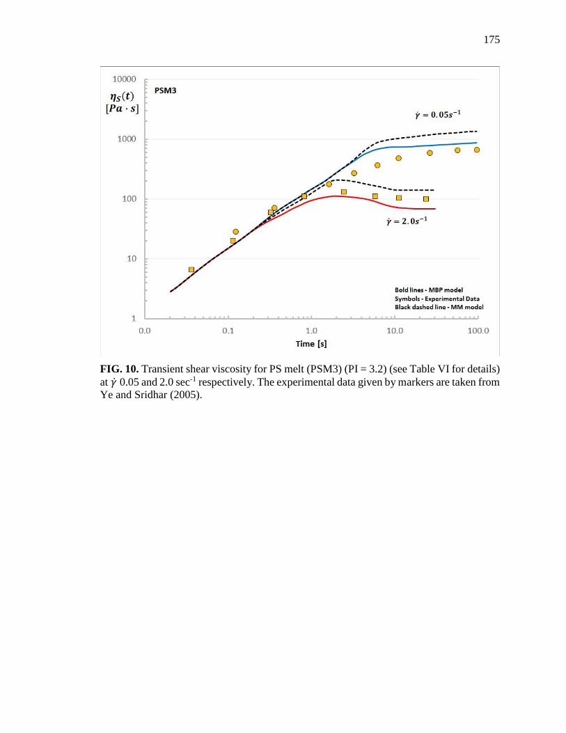
175

FIG. 10. Transient shear viscosity for PS melt (PSM3) (PI = 3.2) (see Table VI for details)

at �� 0.05 and 2.0 sec-1 respectively. The experimental data given by markers are taken from

Ye and Sridhar (2005).

176

FIG. 11. Transient uniaxial extensional viscosity curves of each polymer component for

PS bidisperse melt, PSM1 [Read et al. (2012)], at 𝜀=0.00015, 0.01 and 0.3 s-1, predicted

by MBP model.

177

FIG. 12. Transient fractional stretch, x(t)=(t)/max, curves of each polymer component

for PS bidisperse melt, PSM1 [Read et al. (2012)], at 𝜀=0.00015, 0.01 and 0.3 s-1, predicted

by MBP model.

178

FIG. 13. Transient relative stretch, (t)=L(t)/Leq(t), curves of each polymer component for

PS bidisperse melt, PSM1 [Read et al. (2012)], at 𝜀=0.00015, 0.01 and 0.3 s-1, predicted

by MBP model.

179

FIG. 14. Transient normalized entanglement dynamics curves of each entanglement pair

for PS bidisperse melt, PSM1 [Read et al. (2012)], at 𝜀=0.00015, 0.01 and 0.3 s-1, predicted

by MBP model.

180

FIG. 15. Transient relative stretch curves for Wesslau’s log-normal MWD, for components

1, 4, 7, and 10, at 𝜀=10 s-1, predicted by MBP model.

181

TABLE I. Summary of the experimental data sets used in this study. (PSMW* is not an

experimental data set but a model MWD with log distribution).

Symbol Melt/Solution

Section

used in

Input

parameters

Reference

PSM1 Melt III.A, IV Table II Read et al. (2012)

PSM2 Melt III.A Table III Minegishi et al.

PSM3 Melt III.B Table V Ye & Sridhar (2005)

PSS1 Solution III.A Table II Ye et al. (2003)

PSS2 Solution III.B Table VI

Pattamaprom & Larson

(2003)

PSMW* Melt IV Table VII *Model MWD system

TABLE II. Simulation input values for the uniaxial extension of bidisperse PS melt with

PI = 1.248 (PSM1) [Read et al., (2012)] and bidisperse 7% PS solution (PSS1) [Ye et al.,

(2003)].

Symbol GNo [Pa]

Molecular

weight

[kg/mol]

Weight

fraction τ0

d,i [s] τ0r,i [s] Ne

PSM1 2.46 105 390 0.1402 2.564 104 420.84 20.31

103 0.8598 4.696 102 29.24 5.354

PSS1 6.13 102

2890 0.8 9.40 0.765 12.33

8420 0.2 189.60 5 35.93

182

TABLE III. Simulation input values for the data set PSM2 (PS 686 spiked with MW

3.2106 component; PI=2.33) directly taken from [Mishler and Mead (2013b)], which was

originally obtained from Minegishi et al.

Weight

fraction GN

o [Pa]

Molecular

weight

(kg/mol)

τ0d,i [s] τ0

r,i [s] Ne

0.0186

3.00 105

22.9 1.37 10-3 1.37 10-3 1.762

0.0415 42.3 6.27 10-3 4.69 10-3 3.254

0.0687 67.2 3.02 10-2 1.18 10-2 5.169

0.0961 83.0 0.110 2.53 10-2 0.638

0.117 137 0.340 4.92 10-2 10.538

0.127 184 0.928 8.87 10-2 14.154

0.123 241 2.320 0.152 18.538

0.108 310 5.470 0.252 23.846

0.0879 392 12.100 0.403 30.154

0.0665 490 25.900 0.629 37.692

0.0474 605 53.100 0.959 46.538

0.0321 740 105.000 1.430 56.923

0.0208 897 203.000 2.110 69.000

0.0129 1080 381.000 3.060 83.077

0.00777 1290 697.000 4.360 99.231

0.00452 1530 1.24 103 6.130 117.692

0.00255 1810 2.20 103 8.580 139.231

0.0014 2130 3.83 103 11.900 163.846

7.54 104 2500 6.61 103 16.400 192.308

3.96 104 2910 1.11104 22.200 223.846

0.015 32000 1.53104 26.800 246.154

183

TABLE IV. Summary of which physical effects are included/excluded in each model,

compared in Figure 5.

Model Symbol Equivalent Symbol ED CDFC

MBP MM +ED+CDFC On On

MBP -ED MM +CDFC Off On

MBP -CDFC MM +ED On Off

MBP -ED -CDFC MM Off Off

TABLE V. Simulation input values for shear 7% bidisperse PS solution (PSS2)

[Pattamaprom and Larson (2001)].

TABLE VI. Simulation input values for shear PSM3 [PS melt (P1) (PI=3.5)] [Ye and

Sridhar (2005)].

Weight

fraction GN

o [Pa]

Molecular

weight

(kg/mol)

τ0d,i [s] τ0

r,i [s] Ne

0.002

6.19 102

52.6 1.46 10-4 2.16 10-4 0.225

0.003 76.5 4.47 10-4 4.56 10-4 0.327

0.004 100 1.01 10-3 7.86 10-4 0.429

0.004 120 1.73 10-3 1.13 10-3 0.513

0.01 147 3.17 10-3 1.69 10-3 0.627

0.032 218 1.03 10-3 3.71 10-3 0.930

Symbol GNo [Pa]

Molecular

weight

(kg/mol)

Weight

fraction τ0

d,i [s] τ0r,i [s] Ne

PSS

2.9/8.4 5.20 102

2890 0.6 1.53 0.13 15.21

8420 0.4 31.65 0.6 44.30

184

Table VI. Simulation input values for shear PSM3 [PS melt (P1) (PI=3.5)] [Ye and

Sridhar (2005)] (cont.)

0.009

284 2.29 10-2 6.29 10-3 1.212

0.049 344 4.05 10-2 9.21 10-3 1.467

0.02 442 8.62 10-2 1.52 10-2 1.886

0.122 601 2.17 10-1 2.82 10-2 2.566

0.087 869 6.55 10-1 5.89 10-2 3.708

0.035 978 9.34 10-1 7.46 10-2 4.174

0.179 1410 2.80 1.55 10-1 6.018

0.041 2070 8.83 3.34 10-1 8.826

0.141 2460 1.49 101 4.72 10-1 10.504

0.123 4200 7.38 101 1.37 17.909

0.123 8190 5.48 102 5.23 34.938

0.016 29640 2.60 104 68.5 126.504

TABLE VII. Simulation input values for model generated Wesslau’s log-normal PS melt

MWD with PI = 2.33 and weight avg. MW =2.4 105 (PSMW).

Weight

fraction GN

o [Pa]

Molecular

weight

(kg/mol)

τ0d,i [s] τ0

r,i [s] Ne

3.53 10-4

2.46 105

5.00 2.64 10-6 3.38 10-6 2.60 10-1

2.69 10-3 9.01 1.95 10-5 1.39 10-5 4.69 10-1

0.014 16.2 1.44 10-5 5.67 10-5 8.44 10-1

0.0499 29.2 1.06 10-3 2.33 10-4 1.52

0.123 52.7 7.92 10-3 9.62 10-4 2.74

0.209 94.9 5.85 10-2 3.95 10-3 4.94

0.247 171 0.43 1.62 10-2 8.91

0.2009 308 3.20 6.66 10-2 16.0

0.111 555 23.73 2.74 10-1 28.9

0.0422 1000 175.65 1.12 52.1

185

References

Andreev, M., R.N. Khaliullin, R.J.A. Steenbakkers and J.D. Schieber, “Approximations of

the discrete slip-link model and their effect on nonlinear rheology predictions,” J.

Rheology 57, 535-557 (2013).

Auhl, D., P. Chambon, T.C.B. McLeish and D.J. Read, “Elongational Flow of Blends of

Long and Short Polymers: Effective Stretch Relaxation Time,” Phys. Rev. Lett. 103,

Article 136001 (2009).



dynamics study of a polyethylene melt in steady shear,” Macromolecules 43, 6886-

6906 (2010).

Bremner, T., A. Rudin, and D. G. Cook. “Melt flow index values and molecular weight

distributions of commercial thermoplastics,” Journal of Applied Polymer Science 41,

7‐8 1617-1627 (1990).

Dealy, J. M., and P. C. Saucier. Rheology in plastics quality control. Hanser Publishers,

(2000).

Dealy, J.M. and R.G. Larson, “Structure and rheology of molten polymers: From structure

to flow behavior and back again,” Hanser, Munich (2006).

Dealy, J.M. and WM. K.-W. Tsang, “Structural time dependency in the rheological

behavior of molten polymers,” J. Appl. Poly. Sci. 26, 1149-1158 (1981).

Doi, M., and S.F. Edwards, “The Theory of Polymer Dynamics,” Oxford Science

Publications, (1986).

Eder, G., H. Janeschitz-Kriegl, and S. Liedauer, “Crystallization processes in quiescent and

moving polymer melts under heat transfer conditions,” Progress Polymer Sci. 15, 629–

714 (1990).

186

Everaers, R., S.K. Sukumaran, G.S. Grest, C. Svaneburg, A. Sivasubramanian and K.

Kremers, “Rheology and microscopic topology of entangled polymeric liquids,”

Science 303, 823-827 (2004).

Graham, R.S., A.E. Likhtman, T.C.B. McLeish and S.T. Milner, “Microscopic theory of

linear, entangled polymer chains under rapid deformation including chain stretch and

convective constraint release,” J. Rheology 47, 1171-1200 (2003).

Huang, Q., O. Mednova, H.K. Rasmussen, N.J. Alvarez, A. L. Skov, K. Almdal, and O.

Hassager, “Concentrated Polymer Solutions are Different from Melts: Role of

Entanglement Molecular Weight,” Macromolecules 46, 5026-5035 (2013).

Ianniruberto, G., and G. Marrucci, “Convective constraint release revisited,” J. Rheol. 58,

89-102 (2014).

Larson, R. G., “Constitutive Equations for Polymer Melts and Solutions,” Butterworths,

Boston, (1988).

Likhtman, A. E., and T. C. B. McLeish, ‘‘Quantitative theory for linear dynamics of linear

entangled polymers,’’ Macromolecules 35, 6332–6343 (2002).

Mead, D.W., “Derivation of the “Switch Function” in the Mead-Larson-Doi Theory,”

Rheologica Acta 50, 631-643 (2011).

Mead, D.W., “Development of the “Binary Interaction” Theory for Entangled Polydisperse

Linear polymers,” Rheol. Acta 46, 369-395 (2007).

Mead, D.W., and L. Leal, “The reptation model with chain stretching I) Basic equations

and general properties,” Rheologica Acta 34, 339-360 (1995).

Mead, D.W., D. Yavich and L. Leal, “The reptation model with chain stretching II) Steady

flow properties,” Rheologica Acta 34, 360-383 (1995).

187

Mead, D.W., N. Banerjee and J. Park, “Constitutive model for entangled polymers

incorporating binary entanglement pair dynamics and a configuration dependent

friction coefficient,” J. Rheol 59, 335-363 (2015).

Mead, D.W., R.G. Larson and M. Doi, “A molecular theory for fast flows of entangled

polymers,” Macromolecules 31, 7895-7914 (1998).

Milner, S. T., and T. C. B. McLeish. “Parameter-free theory for stress relaxation in star

polymer melts.” Macromolecules 30, 7 2159-2166 (1997).

Minegishi, A., A. Nishioka, T. Takahashi, Y. Masubuchi, J. Takimoto and K. Koyama,

“The effect of ultrahigh molecular weight polymers on the non-linear response in

uniaxial elongational viscosity,” J. Soc. Rheology Japan 25, 215-216 (1997).

Minegishi, A., A. Nishioka, T. Takahashi, Y. Masubuchi, J. Takimoto and K. Koyama,

“Uniaxial elongational viscosity of PS/a small amount of UHMW-PS blends,”

Rheologica Acta 40, 329-338 (2001).

Minegishi, A., Y. Naka, T. Takahashi, Y. Masubuchi, J. Takimoto and K. Koyama, “Strain

hardening property of polystyrene (PS)/ultrahigh molecular weight (UHMW)-PS

blends,” AIP Conference Proceedings 499, 649-650 (1999).


Flows of Broadly Polydisperse Linear Polymers: Model Development,” J. Non-

Newtonian Fluid Mech. 197, 61-79 (2013a).


Flows of Broadly Polydisperse Linear Polymers: Comparison to Experimental data

Sets,” J. Non-Newtonian Fluid Mech. 197, 80-90 (2013b).

Park, J., D.W. Mead, and M.M. Denn, “Stochastic Simulation of Entangled Polymeric

Liquids in Fast Flows: Microstructure Modification,” J. Rheology 56, 1057-1082

(2012).

188

Pattamaprom, C. and R. G. Larson, “Constraint Release Effects in Monodisperse and

Bidisperse Polystyrenes in Fast Transient Shearing Flows,” Macromolecules 34, 5229-

5237 (2001).

Press, W. H., S. A. Teukolsky, and B. P. Flannery 3rd. “Cambridge University Press; New

York,” Numerical Recipes: The Art of Scientific Computing (2007).

Read, D. J., K. Jagannathan, S. K. Sukumaran and D. Auhl, “A full-chain constitutive

model for bidisperse blends of linear polymers,” J. Rheol. 56, (4), 823-873 (2012).

Rokudai, M., “Influence of shearing history on the rheological properties and

processability of branched polymers,” J. Appl. Poly. Sci. 23, 463-471 (1979).

Watanabe, H., and T. Kotaka, “Viscoelastic properties and relaxation mechanisms of

binary blends of narrow molecular weight distribution

polystyrenes.” Macromolecules 17, 11 2316-2325 (1984).

Ye, X. and T. Sridhar, “Effects of the Polydispersity on Rheological Properties of

Entangled Polystyrene Solutions”, Macromolecules 38, 3442-3449 (2005).

Ye, X., R. G. Larson, C. Pattamaprom, and T. Sridhar, “Extensional properties of

monodisperse and bidisperse polystyrene solutions”, J. Rheol. 47, (2) 443-468 (2003).

189

SECTION

5. CONCLUSION

This dissertation has successfully elucidated the importance of the knowledge of

entangled polymer rheological properties in both the fields of biological science and

polymer processing. The write-up has been organized in three major sections. Firstly, a

review on the mathematical models developed to quantify cytoskeleton mechanical

behavior has been presented; followed by development of constitutive “toy” models to

describe the rheological properties of both monodisperse and polydisperse linear

entangled polymer systems under various deformation conditions.

In the review on mathematical models to study cytoskeleton mechanical

properties, a framework for approaching and understanding the plethora of biopolymer

network models in terms of length scales has been provided. The length scales and their

proper description are important as they are related to the stress components and the

phenomena of interest. Identifying the length scale categories of a model also can give a

quick insight into the advantages and disadvantages of the model and the types of

behaviors and properties described. Conversely, models can be selected based on the

length scale of the phenomena of interest. Models mainly based on the passive dynamics

associated with pure mechanical/rheological responses were focused on. However, there

are models based on different approaches, such as the gel-like model: it was proposed by

Pollock that the cell movement and shape alteration can be described by the phase-

transition mechanism of a gel-like structure (Pollock, 2006). There have been models that

consider the active behaviors which are related with biological responses or structural

190

rearrangement by polymerization/depolymerization. For example, the granular model

considered microtubule rearrangement to describe cell crawling (Maurin et al., 2008).

There have been models which described active behaviors of motor proteins (Chen &

Shenoy, 2011) and growth and remodeling (Na et al., 2007). Although many reviews

have pointed out the need to improve models for active dynamics (Unterberger &

Holzapfel, 2014; Chen et al., 2012; Nava et al., 2014), apparent barriers to that

development are the inherent complexity of the models for passive dynamics and the

need for broader interdisciplinary research including biomedical engineering, medical

science, biophysics, biology, chemistry, materials science, and chemical engineering, etc.

The correct prediction of biopolymer network mechanical/rheological properties is

important in many biomedical applications associated with biopolymer networks.

Therefore, the framework provided by this review is expected to promote various studies

on biopolymer networks (Banerjee & Park, 2015).

Moving on from the field of medicine to that of polymer processing, the research

attempted to understand and answer some of the persisting questions regarding linear

monodisperse entangled polymer systems under fast non-linear deformation conditions.

In that effort a mathematically and computationally simple “toy” molecular

model that incorporates ED, CDFC, and CCR into the base DEMG “toy” model, the

MBP model for monodisperse entangled polymers was constructed. This model is a

natural next step in the systematic progression of increasingly detailed and complex

molecular models for entangled linear flexible polymers. The constitutive equation

developed for monodisperse polymer melt or an entangled semi-dilute solution has three

191

major components (see equation (1)): 1) A quantitative description of the orientation

dynamics, 2) a quantitative description of the stretch dynamics, and 3) a quantitative

description of the entanglement dynamics (which are manifested through the nonlinear

modulus tGN). All the three components are coupled together and nonlinear. The effect

of CDFC has been incorporated in the description of the time scales (Mead et al., 2015).

dynamicsnOrientatio

tube

dynamicsStretch

dynamicsnglementEnta

N tSttGt 23 (1)

The new MBP model generates extensional flow curves that are monotonically

thinning (with a small “kink” near 1, eqs ) for monodisperse PS melts that are

qualitatively consistent with the experiment. The results are sensitive to the specific

functional form of the CDFC used. For monodisperse PS solutions, the effects of CDFC

are effectively diluted out and the classical tube model ladle shaped extensional flow

curve is generated. The simulation results strongly suggest that CDFC is important in the

prediction of rheological properties in nonlinear extensional flows of monodisperse PS

melts. CCR is detrimental to the predictions in extensional flows but is important for the

rheological properties in shear flows (Mead et al., 2015).

A plausible explanation as to why the DEMG-cdfc model yields a monotonically

thinning flow curve of monodisperse PS melts that are approximately equivalent to those

predicted by the new MBP-xccr model (i.e. DEMG with ED “on”, CDFC “on” and CCR

“off”) is also provided. This suspicious coincidence masks the underlying details that are

actually occurring in fast nonlinear flows of entangled polymers. The new model

192

simultaneously captures nonlinear flows and the entanglement microstructure

modification that occurs in these fast flows (Mead et al., 2015).

Furthermore, the knowledge of the melt entanglement density following polymer

shaping operations (finite deformations) is crucially important with respect to

determining the ultimate mechanical properties of the part. Hence, the information

gleaned from molecular models with ED, such as the MBP model, is directly relevant to

polymer processing operations (Mead et al., 2015).

The next endeavor is to generalize the new MBP model to polydisperse systems.

Having a generally applicable model for polydisperse systems that is easy to code and

fast to execute has many practical applications in analytic rheology. The MBP

monodisperse model and Mishler and Mead’s (2013a, 2013b) “diluted stretch tube”

theory is combined together to develop the MBP polydisperse model. The concepts of

CDFC and ED are sustained in the MBP polydisperse “toy” model.

The MBP polydisperse model can correctly predict the PS bi-blend both melt and

solution behavior under uniaxial extension, defining each component’s effect on the

overall system. It can be concluded that due to the solution-like behavior of some of the

entanglements, the CDFC effect weakens and is not important in defining the overall

viscosity of the system. The CDFC effect is similar to what observed in case of

monodisperse solution systems (Mead et al., 2015).

Entanglement dynamics (ED), on the other hand, proved to be very important

physics in defining the system. This observation is not unpredictable as the entanglement

193

structure is very complex for a polydisperse system. With different time scales, the strong

effect of ED is imperative. The model can also predict the individual effects due to the

short and the long components of the system. It is observed, that the deviation that occurs

in the transient viscosity from LVE (strain hardening), is due to the commencement of

stretch in the long chain component. Further increase in extension rates causes the shorter

chain to start stretching and then the overall viscosity is scaled both by longer and shorter

chain.

The wide MWD PS 686, a most probable MWD and the model generated

Wesslau’s log-normal MWD are simulated to understand the effect of the high molecular

weight component on the overall viscosity of the system. The model can predict the

experimental behavior for PS 686 very accurately. For both the PS 686 and Wesslau’s

log-normal MWD, the strain hardening is observed exactly at the point when the high

molecular weight component begins stretching. The model can also correctly predict the

shear flow transient and steady state (shear viscosity, shear stress and first normal stress

difference) behavior for both the bidisperse solution and large MWD melt, again

confirming that ED is important to both qualitatively and quantitatively describe the

properties. Even in shear melt and solution systems, CDFC is found to be inconsequent.

It has long been known that a polymer melt’s rheological properties reflect the

underlying fluid microstructure (Dealy and Saucier, 2000; Dealy and Larson, 2006).

Microstructure here refers to the MWD, entanglement density and long chain branching.

Consequently, rheology is commonly used in industry to characterize polymer resins

194

using relatively crude rheological criteria such as the Melt Flow Index (MFI) (Bremner et

al., 1990).

Figure 5.1. Analytic rheology scheme.

Such rheological criteria were until recently largely based on empiricism rather

than sound theory. However, molecular rheology has advanced to the point where it is

now possible to definitively and quantitatively characterize commercial polymer resins

from their rheology alone. These ideas form the motivation and basis of Analytic

Rheology as a science. Thus, having a generally applicable model for polydisperse

195

systems that is easy to code and fast to execute has many practical applications in

analytic rheology. Analytic rheology is the prediction of the molecular weight

distribution of the system from the viscosity and stress data. Figure 5.1, gives a glimpse

of the analytic rheology procedure.

APPENDIX A.

TRACE OF ORIENTATION TENSOR ( tSijtube,

) FOR THE MBP

POLYDISPERSE “TOY” MODEL

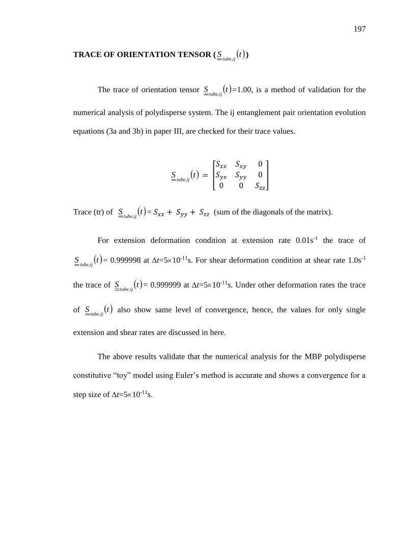
197

TRACE OF ORIENTATION TENSOR ( tSijtube,

)

The trace of orientation tensor tSijtube,

=1.00, is a method of validation for the

numerical analysis of polydisperse system. The ij entanglement pair orientation evolution

equations (3a and 3b) in paper III, are checked for their trace values.

tSijtube,

= [

𝑆𝑥𝑥 𝑆𝑥𝑦 0

𝑆𝑦𝑥 𝑆𝑦𝑦 0

0 0 𝑆𝑧𝑧

]

Trace (tr) of tSijtube,

= 𝑆𝑥𝑥 + 𝑆𝑦𝑦 + 𝑆𝑧𝑧 (sum of the diagonals of the matrix).

For extension deformation condition at extension rate 0.01s-1 the trace of

tSijtube,

= 0.999998 at t=510-11s. For shear deformation condition at shear rate 1.0s-1

the trace of tSijtube,

= 0.999999 at t=510-11s. Under other deformation rates the trace

of tSijtube,

also show same level of convergence, hence, the values for only single

extension and shear rates are discussed in here.

The above results validate that the numerical analysis for the MBP polydisperse

constitutive “toy” model using Euler’s method is accurate and shows a convergence for a

step size of t=510-11s.

APPENDIX B.

ADDITIONAL FIGURES AND TABLES FOR THE MBP POLYDISPERSE

“TOY” MODEL

199

B.1. Component entanglement dynamics results:

The importance of entanglement dynamics (ED) to describe the polydisperse

system has been discussed in detail in paper III (Sections III.A and IV). Figure B.1 shows

the transient normalized entanglement dynamics curve for the short and the long chain

components, for PSM1 (see Table 2., in paper III Section III.A for details) at extension

rates έ 0.00015, 0.01 and 0.3 sec-1. This shows the drop in the number of entanglements

in long and short chains w.r.t to the equilibrium number of entanglements.

Figure B.1. Transient normalized entanglement dynamics curve for PSM1 at έ 0.00015,

0.01 and 0.3 sec-1 showing the short and long chain entanglement dynamics.

200

As can be seen from Figure B.1, the number of entanglements on the longer chain

component falls of more than the short chain components. This is because the

entanglements on long-long components fall off to a larger extend compared to the long-

short, short-short and short-long which can be seen from Figure 14, in Paper III. The

reason behind the faster disentanglement of long-long components as discussed is due to

the reduced re-entanglement or formation of new entanglements for the long-long

components.

Figure B.2. Transient normalized entanglement dynamics curve (𝑁_𝑖𝑗 (𝑡)) ⁄ 𝑁_𝑖 )for

PSM1 at έ 0.00015, 0.01 and 0.3 sec-1 showing the short and long chain entanglement

dynamics.

201

Figure B.3. Transient normalized entanglement dynamics curve (𝑁_𝑖𝑗 (𝑡)) ⁄ 𝑁_𝑒𝑖 )for


dynamics.

In order to investigate the entanglement dynamics behavior of each of the

individual components at different extension rates, different normalized curves have been

plotted. Figure B.2. shows the Transient normalized entanglement dynamics curve

(𝑁_𝑖𝑗 (𝑡)) ⁄ 𝑁_𝑖 )for PSM1 at έ 0.00015, 0.01 and 0.3 sec-1. Similarly, Figure B.3 and

B.4 show the Transient normalized entanglement dynamics curve (𝑁_𝑖𝑗 (𝑡)) ⁄ 𝑁_𝑒𝑖 ) and

(𝑁_𝑖𝑗 (𝑡)) ⁄ ((𝑁_𝑖 (𝑡) ∗ 𝑤_𝑗)) or PSM1 respectively. Each of these curves show how

the number of entanglements on the chain is changing with time.

202

Figure B.4. Transient normalized entanglement dynamics curve (𝑁_𝑖𝑗 (𝑡)) ⁄ ((𝑁_𝑖 (𝑡) ∗

𝑤_𝑗)) or PSM1 at έ 0.00015, 0.01 and 0.3 sec-1 showing the short and long chain

entanglement dynamics.

B.2. Steady state uniaxial extension melt and shear solution results:

Along with the transient behavior, the steady state behavior of PSM1 under

uniaxial extension and of PSS2 under shear is of interest. Figure B.5 gives the steady

uniaxial extensional viscosity curve for PSM1 (see Table 2., in paper III for details) along

with the short chain and the long chain contributions. The observations in close

agreement with the experimental results from Read et al. (2012). One can again see that

with increase in extension rates, the contributions of the long chains increases as the it

203

starts stretching at 𝜀 > ~0.002 =1

𝜏𝑟−𝑙𝑜𝑛𝑔. On further increasing the extension rates, the

short chain starts stretching 𝜀 > ~0.04 =1

𝜏𝑟−𝑠ℎ𝑜𝑟𝑡, and its contribution becomes more

prominent. For high extension rate condition both the short and the long chains contribute

equally to the overall viscosity of the system. The stretching effects of the individual

components have been more clearly described in paper III, Section IV.

Figure B.5. Steady state extensional viscosity curve for PS bidisperse melt (see Table 2.,

in paper III for details). The long and short chain component effects are given by dashed

and dotted lines respectively. The experimental data given by markers are taken from

Read et al. (2012).

204

Figure B.6 shows the steady state shear viscosity and first normal stress difference

vs shear rate curve, for PSS2 (see Table 5., in paper III for details). The MBP predictions

are in close agreement with the experimental results from Pattamaprom and Larson

(2001). As expected, the shear viscosity for polydisperse solution system monotonically

reduces with increase in shear rate, whereas the first normal stress difference shows a

monotonic increase with shear rate.

Figure B.6. Steady state shear viscosity and first normal stress difference vs shear rate

curve difference for 7% PS bidisperse solution (see Table 5., in paper III for details). The

experimental data given by markers are taken from Pattamaprom and Larson (2001).

205

B.3. [PS 686] and PSMW [Wesslau’s log-normal] MWD under uniaxial extension

results:

The effect of higher molecular weight component, on the overall viscosity of the

system, for wide molecular weight distribution (MWD), is of interest. The PSM2 (PS 686

melt system spiked with 3.2106 MW component (Mishler & Mead, 2013)) (see Table 3.,

in paper III for details) is simulated and the results (see Figure 4) are discussed in paper

III, Section III.A. Figure B.7, shows the transient relative stretch curves for components,

9, 13, and 21 (see Table 3., in paper III for details) at extension rate 0.572sec-1.

Figure B.7. Relative stretch curve for PSM2 (PS 686, for components (9, 13 and 21)) (see

Table 3., in paper III for details) at έ 0.572 sec-1.

206

It can be clearly seen that the strain hardening observed in the system (see Figure

4., in paper III for the transient viscosity curve) is due to stretch occurring in the high

molecular weight component.

The PSMW (Wesslau’s log-normal 10 components PS melt MWD (PI = 2.33))

for uniaxial extension deformation (see Table 7., in paper III for details) is a model

generated MWD which is simulated to validate the stretching effects of high molecular

weight components on the overall viscosity of the system under high uniaxial extension

deformation.

Figure B.8. Transient extensional viscosity curve for PSMW (Wesslau’s log-normal PS

melt MWD) (see Table 7., in paper III for details) at extension rates 0.001, 1.0 and 10

sec-1. The LVE is given by grey dashed line.

207

Figure B.8. shows the transient extensional viscosity curves at extension rates

0.001, 1.0 and 10 sec-1 respectively. The effects of the stretching in the high molecular

weight components have been discussed in paper III, Section IV (see Figure 14).

B.4. Most probable MWD results:

The most probable two components MWD is generated using the code. Figure

B.9. shows the transient extensional viscosity curve at extension rates 0.001, 1.0 and 10

sec-1 respectively.

Figure B.9. Transient extensional viscosity curve for most probable PS melt MWD (see

Table B.1. for details) at extension rates 0.001, 1.0 and 10 sec-1. The LVE is given by

grey dashed line.

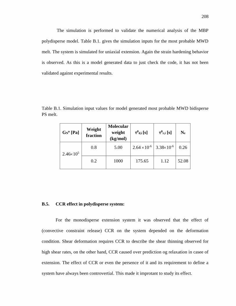
208

The simulation is performed to validate the numerical analysis of the MBP

polydisperse model. Table B.1. gives the simulation inputs for the most probable MWD

melt. The system is simulated for uniaxial extension. Again the strain hardening behavior

is observed. As this is a model generated data to just check the code, it has not been

validated against experimental results.

Table B.1. Simulation input values for model generated most probable MWD bidisperse

PS melt.

GNo [Pa]

Weight

fraction

Molecular

weight

(kg/mol)

τ0d,i [s] τ0

r,i [s] Ne

2.46105

0.8 5.00 2.64 10-6 3.3810-6 0.26

0.2 1000 175.65 1.12 52.08

B.5. CCR effect in polydisperse system:

For the monodisperse extension system it was observed that the effect of

(convective constraint release) CCR on the system depended on the deformation

condition. Shear deformation requires CCR to describe the shear thinning observed for

high shear rates, on the other hand, CCR caused over prediction og relaxation in casee of

extension. The effect of CCR or even the persence of it and its requirement to define a

system have always been controvertial. This made it improtant to study its effect.

209

Fig B.10. Transient extensional viscosity for PS melt (PSM1) at 0.3 s-1 extension rate for

different simulation combinations to check the effect of the individual physics.

To check the effect of CCR in case of polydisperse melt extension (PSM1) and

see how CCR is effecting the system MBP xCCR. Figure B.10 shows the individual effect

of ED, CDFC and CCR. The effects of ED and CDFC have been discussed in detail in

Paper III. On turning “off” CCR, it can be seen that the curve deviates from the

experimental results and the behavior is similar to that of MBP without CDFC. Thus one

can conclude that CCR again have a week effect on the overall behavior of the system.

The behavior is thus similar to that of the monodisperse extension melt systems when

210

CCR becomed ineefective due to the loss of ttopological constraint when the system gets

highly oriented.

B.6. Diluted tube Stretch, Maximum relative stretch and CDFC

Figure B.11 shows the comparison bbetween the relative stretch in the primary

and the diluted tube for bidisperse PS melt (PSM1) under extension rates έ 0.00015, 0.01

and 0.3 sec-1. It can be seen that as the extension rates increases, the stretching in the

diluted tube becomes more prominent compared to that of the primary tube.

Figure B.11. Transient normalized entanglement dynamics curve (𝑁_𝑖𝑗 (𝑡)) ⁄ 𝑁_𝑒𝑖 )for


dynamics.

211

The diluted tube for the longer chain component is stretched more than the

primary tube. This may be becarse the siluted tube is defined by only viable components

whereas, the primary tube is defined by all the entanglements present in the sytem. This

allows the diluted tube to unravel more and get stretched.

Figure B.12. shows the maximum relative stretch for diluted tube for bidisperse

PS melt (PSM1) under extension rates έ 0.00015, 0.01 and 0.3 sec-1. Here one can see

that the diluted tube starts unravelling under high extension rates. The chain start to

stretch and the back bends and loops in the chain gets straightened.

Figure B.12. Transient maximum relative stretch for diluted tube for PSM1 at έ 0.00015,

0.01 and 0.3 sec-1 showing the short and long chain entanglement dynamics.

212

Figure B.13. Transient CDFC for PSM1 at έ 0.00015, 0.01 and 0.3 sec-1 showing the

short and long chain entanglement dynamics.

Figure B.13. shows the transient CDFC effect PSM1 at έ 0.00015, 0.01 and 0.3

sec-1. From this curve one can observe that the with increase in extension rate, the long

chain gets effected first, then both long and short chains showing CDFC due to

orientation. Though CDFC effect is there, the reduction due to CDFC is not high and thus

their effect on the overall behavior of the system is not prominent.

213

REFERENCES

Andreev, M., Khaliullin, R. N., Steenbakkers, R. J. A., and Schieber J. D. “Approximations

of the discrete slip-link model and their effect on nonlinear rheology

predictions,” Journal of Rheology, 57, 2 (2013) 535-557.

Auhl, D., Chambon, P., McLeish, T. C. B., and Read, D. J. “Elongational flow of blends

of long and short polymers: Effective stretch relaxation time,” Physical review

letters, 103, 13 (2009) 136001(4).



dynamics study of a polyethylene melt in steady shear”, Macromolecules 43, (2010)

6886-6906.

Banerjee, N., and Park, J. “Modeling and simulation of biopolymer networks:

Classification of the cytoskeleton models according to multiple scales,” Korean Journal

of Chemical Engineering, 32, 7 (2015) 1207-1217.

Barkema, G. T., Panja, D., Van Leeuwen, J. M. J. “Structural modes of a polymer in the

repton model,” The Journal of Chemical Physics, 134, 15 (2011) 154901.

Bremner, T., A. Rudin, and D. G. Cook. “Melt flow index values and molecular weight

distributions of commercial thermoplastics,” Journal of Applied Polymer Science 41,

7‐8 (1990) 1617-1627.

Chen, P., and V. B. Shenoy. “Strain stiffening induced by molecular motors in active

crosslinked biopolymer networks,” Soft Matter, 7 (2011) 355-358.

Chen, T. J., C. C. Wu, and F. C. Su. “Mechanical models of the cellular cytoskeletal

network for the analysis of intracellular mechanical properties and force distributions:

A review,” Medical engineering & physics, 34, 10 (2012) 1375-1386.

De Gennes, P. G. “Reptation of a Polymer Chain in the Presence of Fixed Obstacles,”

Journal of Chemical Physics, 55, 2 (1971) 572-579.

De Gennes, P. G. “Reptation of stars,” Journal de Physique, 36, 12 (1975) 1199-1203.

214

Dealy, J. M., and P. C. Saucier. Rheology in plastics quality control. Hanser Publishers,

(2000).

Dealy, J.M. and R.G. Larson, “Structure and rheology of molten polymers: From structure

to flow behavior and back again,” Hanser, Munich (2006).

Des Cloizeaux, J. “Double reptation vs. simple reptation in polymer melts,” EPL

(Europhysics Letters), 5, 5 (1988) 437-442.

Des Cloizeaux, J. “Relaxation and viscosity anomaly of melts made of long entangled

polymers: time-dependent reptation,” Macromolecules, 23, 21 (1990) 4678-4687.

Doi M., and Kuzuu, N. Y. “Rheology of star polymers in concentrated solutions and

melts,” Journal of Polymer Science: Polymer Letters Edition, 18, 12 (1980) 775-780.

Doi, M. and Edwards, S. F. The theory of polymer dynamics. Oxford University Press,

New York, (1986).

Doi, M., and Edwards, S. F. “Dynamics of concentrated polymer systems. Part 1. -

Brownian motion in the equilibrium state,” Journal of the Chemical Society, Faraday

Transactions 2: Molecular and Chemical Physics, 74 (1978a) 1789-1801.

Doi, M., and Edwards, S. F. “Dynamics of concentrated polymer systems. Part 2. -

Molecular motion under flow,” Journal of the Chemical Society, Faraday Transactions

2: Molecular and Chemical Physics, 74 (1978b) 1802-1817.

Doi, M., and Edwards, S. F. “Dynamics of concentrated polymer systems. Part 4.-

Rheological properties,” Journal of the Chemical Society, Faraday Transactions 2:

Molecular and Chemical Physics, 75 (1979) 38-54.

G. H. Pollack, in Cytoskeletal Mechanics - Models and Measurements in Cell Dynamics,

M. R. K. Mofrad, and R. D. Kamm Eds., Cambridge University Press (2006).

Ianniruberto, G., and Marrucci, G. “On compatibility of the Cox-Merz rule with the model

of Doi and Edwards,” Journal of Non-Newtonian fluid mechanics, 65, 2 (1996) 241-

246.

215

Ianniruberto, G., Brasiello A., and Marrucci, G. “Simulations of fast shear flows of PS

oligomers confirm monomeric friction reduction in fast elongational flows of

monodisperse PS melts as indicated by rheooptical data,” Macromolecules, 45, 19

(2012) 8058-8066.

Kremer, K., and Grest, G. S. “Dynamics of entangled linear polymer melts: A molecular‐

dynamics simulation,” The Journal of Chemical Physics, 92, 8 (1990) 5057-5086.

Kuhn, W. “über die gestalt fadenförmiger moleküle in lösungen,” Kolloid-Zeitschrift, 68,

1 (1934) 2-15.

Larson, R. G. The Structure and Rheology of Complex Fluids. Oxford University Press,

New York, 1999.

Lodge, T. P., Rotstein, N. A., and Prager, S. “Dynamics of entangled polymer liquids: Do

linear chains reptate?,” Advances in Chemical Physics, 79 (1992) 1-132.

Marrucci, G. “Dynamics of entanglements: A nonlinear model consistent with the Cox-

Merz rule,” Journal of non-Newtonian fluid mechanics, 62, 2 (1996) 279-289.

Marrucci, G. and Ianniruberto, G. “Effect of flow on topological interactions in polymers,”

In Macromolecular symposia, Hüthig & Wepf Verlag, 117, 1 (1997) 233-240.

Marrucci, G., and Grizzuti, N. “Fast flows of concentrated polymers-predictions of the

tube model on chain stretching,” Gazzetta Chimica Italiana, 118, 3 (1988) 179-185.

Maurin, B., P. Canadas, H. Baudriller, P. Montcourrier, and N. Bettache. “Mechanical

model of cytoskeleton structuration during cell adhesion and spreading,” Journal of

biomechanics, 41, 9 (2008) 2036-2041.

McLeish, T. C. B. “Tube theory of entangled polymer dynamics,” Advances in Physics,

51, 6 (2002) 1379-1527.

Mead, D. W. “Determination of molecular weight distributions of linear flexible polymers

from linear viscoelastic material functions,” Journal of Rheology, 38, 6 (1994) 1797-

1827.

Mead, D. W. “Development of the “binary interaction” theory for entangled polydisperse

linear polymers,” Rheologica acta, 46, 3 (2007) 369-395.

216

Mead, D. W., Banerjee, N. and Park, J. “Constitutive model for entangled polymers

incorporating binary entanglement pair dynamics and a configuration dependent

friction coefficient,” Journal of Rheology, 59, 2 (2015) 335-363.

Mead, D. W., Larson R. G., and Doi M., “A Molecular Theory for Fast Flows of Entangled

Polymers,” Macromolecules, 31 (1998) 7895-7914.


Flows of Broadly Polydisperse Linear Polymers: Comparison to Experimental data Sets,”

J. Non-Newtonian Fluid Mechanics, 197 (2013b) 80-90.

Mishler, S.D. and Mead, D. W. “Application of the MLD “Toy” Model to Extensional

Flows of Broadly Polydisperse Linear Polymers: Model Development,” Journal of

Non-Newtonian Fluid Mechanics, 197 (2013a) 61-79.

Na, S., G. A. Meininger, and J. D. Humphrey. “A theoretical model for F-actin remodeling

in vascular smooth muscle cells subjected to cyclic stretch,” Journal of theoretical

biology, 246, 1 (2007) 87-99.

Nava, M. M., M. T. Raimondi, and R. Pietrabissa. “Bio-chemo-mechanical models for

nuclear deformation in adherent eukaryotic cells,” Biomechanics and modeling in

mechanobiology, 13, 5 (2014) 929-943.

Park, J., Mead, D. W. and Morton, M. D. “Stochastic simulation of entangled polymeric

liquids in fast flows: Microstructure modification,” Journal of Rheology, 56, 5 (2012)

1-25.

Pattamaprom, C. and R. G. Larson, “Constraint Release Effects in Monodisperse and

Bidisperse Polystyrenes in Fast Transient Shearing Flows,” Macromolecules 34, (2001)

5229-5237.

Pearson, D. S. “Recent advances in the molecular aspects of polymer

viscoelasticity,” Rubber chemistry and technology, 60, 3 (1987) 439-496.

Pearson, D., Herbolzheimer, E., Grizzuti, N., and Marrucci, G. “Transient behavior of

entangled polymers at high shear rates,” Journal of Polymer Science Part B: Polymer

Physics, 29, 13 (1991) 1589-1597.

217

Read, D. J., K. Jagannathan, S. K. Sukumaran and D. Auhl, “A full-chain constitutive

model for bidisperse blends of linear polymers,” J. Rheol. 56, (4), (2012) 823-873.

Rouse Jr, P. E. “A theory of the linear viscoelastic properties of dilute solutions of coiling

polymers,” The Journal of Chemical Physics, 21, 7 (1953) 1272-1280.

Rubinstein, M. “Discretized model of entangled-polymer dynamics,” Physical Review

Letters, 59, 17 (1987) 1946–1949.

Rubinstein, M. and Colby, R. H. Polymer Physics. 1st ed. Oxford University Press, UK,

(2003).

Rubinstein, M., and Colby, R. H. “Self‐consistent theory of polydisperse entangled

polymers: Linear viscoelasticity of binary blends,” The Journal of chemical

physics, 89, 8 (1988) 5291-5306.

Tsenoglou, C. "Viscoelasticity of binary homopolymer blends." In abstracts of Papers of

the American Chemical Society, 1155 16th St, NW, Washington, DC 20036: Amer.

Chemical Soc., 194 (1987) 219-POLY.

Tsenoglou, C. “Molecular weight polydispersity effects on the viscoelasticity of entangled

linear polymers,” Macromolecules, 24, 8 (1991) 1762-1767.

Unterberger, M. J., and G. A. Holzapfel. “Advances in the mechanical modeling of

filamentous actin and its cross-linked networks on multiple scales,” Biomechanics and

modeling in mechanobiology, 13, 6 (2014) 1155-1174.

Vivoy, J. L., Rubinstein, M., and Colby, R. H. “Constraint release in polymer melts: tube

reorganization versus tube dilation,” Macromolecules, 24, 12 (1991) 3587-3596.

Wasserman, S. H., and Graessley, W. W. “Effects of polydispersity on linear viscoelasticity

in entangled polymer melts,” Journal of Rheology, 36, 4 (1992) 543-572.

Wingstrand, S. L., Alvarez, N. J., Huang, Q., and Hassager, O. “Linear and nonlinear

universality in the rheology of polymer melts and solutions,” Physical review

letters, 115, 7 (2015) 078302(5).

Xu, F., Morton, M. D. and Schieber J. D. “A full chain stochastic tube model for entangled

melts and solutions of linear polymers,” Journal of Rheology, 50, 4 (2006) 477-494.

218

Yaoita, T., Isaki, T., Masubuchi, Y., Watanabe, H., Ianniruberto, G. and Marrucci, G.

‘Primitive chain network simulation of elongational flows of entangled linear chains:

stretch/orientation-induced reduction of monomeric friction,” Macromolecules, 45, 6

(2012) 2773-2782.

Yaoita, T., Masubuchi, Y., and Watanabe, H. "Concept of stretch/orientation-induced

friction reduction tested with a simple molecular constitutive equation." Journal of the

Society of Rheology, Japan, 42, 3 (2014) 207-213.

Ylitalo, C. M., Fuller, G. G., Abetz, V., Stadler, R., and Pearson, D. S. “Relaxation

dynamics of selected polymer chain segments and comparison with theoretical

models,” Rheologica Acta, 29, 6 (1990) 543-555.

Zimm, B. H. “Dynamics of polymer molecules in dilute solution: viscoelasticity, flow

birefringence and dielectric loss,” The journal of chemical physics, 24, 2 (1956) 269-

278.

219

VITA

Nilanjana Banerjee was born in Kolkata, West Bengal, India, on February 20, 1986.

In May 2008 she received her Bachelor of Technology (B.Tech) with Honors in Chemical

Engineering from the Nirma Institute of Technology, Nirma University, Ahmedabad,

Gujarat, India. She was also awarded the best student award during the Bachelor degree

commencement ceremony. She did her summer training at Larson and Toubro – Chiyoda,

Vadodara, India during the summer of 2007.

She received her Master’s in Chemical Engineering (M.Chem.Engg.) with Honors

from Institute of Chemical Technology, Mumbai University (formerly UDCT), Mumbai,

India, in June 2010. Her Master’s thesis was nominated for the ISTE/IPCL best Master’s

thesis award in 2010.

In December 2010, she joined the Chemical Engineering Department of Maharaja

Sayajirao University, Vadodara, Gujarat, India, as a lecturer and taught till April, 2012. In

May 2016, she received her Ph.D. in Chemical Engineering from the Missouri University

of Science and Technology, Rolla, Missouri, USA. She has published conference and

journal papers, some of which are listed with the references of this research.

Nilanjana Banerjee has been a member of the American Institute of Chemical

Engineering (AIChE) since 2013. She has been a member of the Institute of Engineering

and Technology (IET) since 2015.

Documents

Modeling of rheological properties for entangled polymer