Modeling Land-Use Changes in the South Nation Watershed ... Khoury_Antoun... · Modeling Land-Use Changes in the South Nation Watershed using Dyna-CLUE by Antoun El Khoury A Thesis

Modeling Land-Use Changes in the South Nation Watershed

using Dyna-CLUE

by

Antoun El Khoury

A Thesis

Presented to the University of Ottawa in Partial Fulfillment of the Requirements for

Master of Applied Science in Environmental Engineering

Department of Civil Engineering

University of Ottawa

Ottawa, Canada

K1N 6N5

The M.A.Sc. in Environmental Engineering

is a joint program with Carleton University administered by

The Ottawa-Carleton Institute for Environmental Engineering

© Antoun El Khoury, Canada, 2012

To my wife Reine and my son Peter

i

ACKNOWLEDGEMENT

I would like to express my deepest appreciation to my supervisor Dr. Ousmane Seidou

and my co-supervisor Dr. Majid Mohammadian; without their guidance and persistent help

this research work would not have been possible.

My deepest gratitude for Dr. Robert Delatolla, Dr. Bahram Daneshfar, Dr. Colin Rennie,

and Dr. Mamadou Fall for serving on my graduate committee and providing me with

valuable suggestions.

Special acknowledgements to the developers of the Dyna-CLUE model, especially

Dr. Peter Verburg (University of Wageningen, The Netherlands) for his valuable time

responding to my inquiries which allowed me to better understand how the model works.

I would like to thank my friends: Dr. Mohamed Abdallah & Dr-to-be. Ketvara Sittichok

and Omar Al-Attas who helped me during my study.

Last but not least, I am thankful to the University of Ottawa for having the opportunity

to be enrolled in the Master's program in the Department of Environmental Engineering.

ii

ABSTRACT

The South Nation watershed is located in Eastern Ontario, Canada and managed under the

authority of the South Nation Conservation (SNC). The watershed covers an area of 400,000

hectares with four dominant categories of land-use classes (60% agriculture, 34% forest, 5%

mixed urban, and 1% other). Water quality is a great concern for the SNC as many

anthropogenic activities generate harmful pollutants (such as heavy metals, nitrogen,

phosphorus, and pesticides) that are discharged to the river through surface and groundwater

flow. The discharge patterns of these pollutants are mainly driven by land-use distribution

within the watershed which has been constantly evolving with urbanization and

intensification of agriculture. Major changes in land-uses can potentially offset current SNC

efforts to mitigate water pollution.

The objective of the current study is to predict land-use series of maps for the South Nation

watershed starting from 1991 to 2020. The prediction is carried out using the land-use

allocation algorithm of the Dyna-CLUE (Dynamic Conversion of Land-Use and its Effects)

model which is implemented for local regions. Dyna-CLUE is a spatially explicit hybrid

land-use allocation model that combines estimation and simulation models, and its allocation

procedures predict future trends of land-use surface (estimated from historical trends). The

binary logistic regression is used to link preferences of land-use classes and potential

demographic and geographic driving factors. Expert judgment was used to select a set of

spatial driving factors believed to be responsible for changes in land-use distribution in the

South Nation watershed. Three different scenarios for future development of the region were

considered, with different initial conditions and conversion restrictions. The simulation

iii

results were evaluated using visual and statistical validation techniques to assess the

performance of the model in generating maps similar to reality.

The Dyna-CLUE model was successfully applied to the South Nation watershed. It was

observed that the simulated maps generated from the model were in good agreement with the

reality maps. This was confirmed through statistical validation via map pair analysis (error

matrix) used to assess the overall accuracy of the model predictions. Results showed that the

model was sensitive to land-use restrictions. Such type of modeling can be valuable for

assessing the land-use changes at the local level, and setting up a decision support system for

the South Nation Conservation towards sustainable land-use management in the watershed.

Better results are expected to be achieved with more reliable datasets (i.e., accurate

classification of land-use types in reality maps). Data availability and quality were the main

obstacles that faced this research work. Our work has the merit to be the first application of

CLUE model in Eastern Ontario.

iv

TABLE OF CONTENTS

ACKNOWLEDGEMENT ...................................................................................................................................I

ABSTRACT ........................................................................................................................................................ II

TABLE OF CONTENTS .................................................................................................................................. IV

LIST OF FIGURES ........................................................................................................................................ VIII

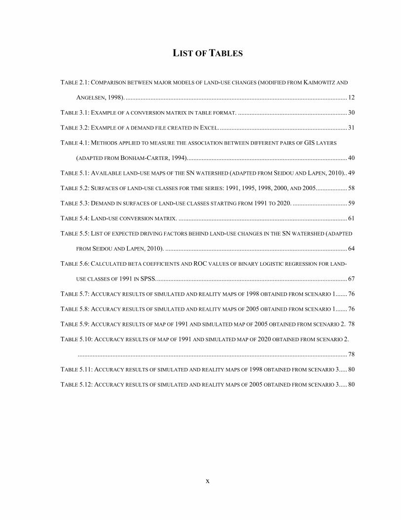
LIST OF TABLES .............................................................................................................................................. X

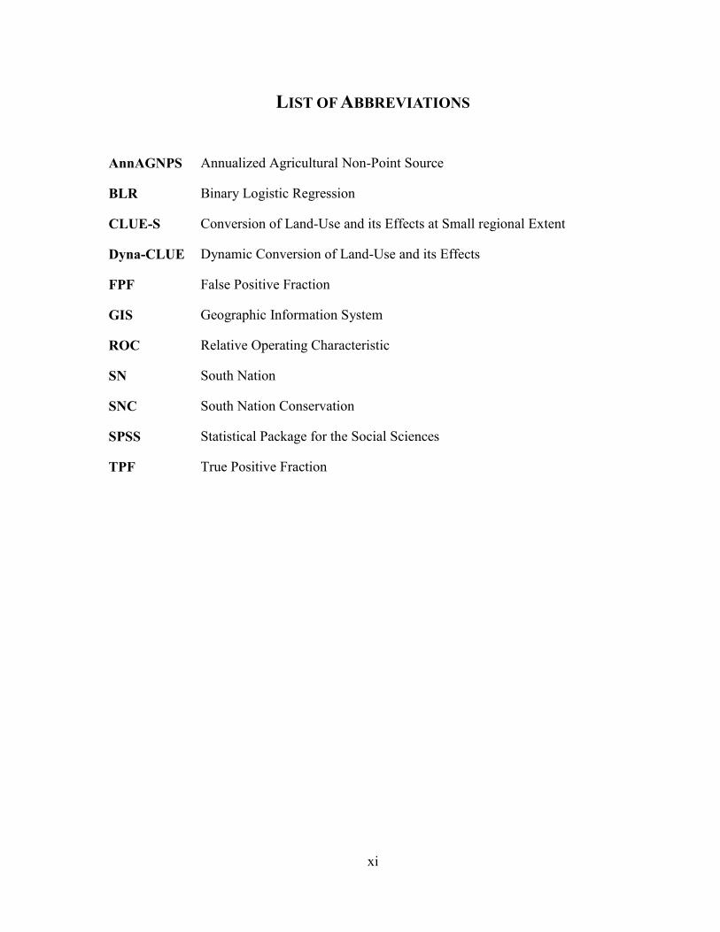
LIST OF ABBREVIATIONS ........................................................................................................................... XI

CHAPTER 1 INTRODUCTION ....................................................................................................................... 1

1.1. BACKGROUND ..................................................................................................................................... 1

1.2. TYPES OF MODELS .............................................................................................................................. 2

1.3. RESEARCH PROBLEM AND OBJECTIVES ............................................................................................... 2

1.4. SPECIFIC RESEARCH OBJECTIVE .......................................................................................................... 3

1.5. METHODOLOGY................................................................................................................................... 4

1.6. ORGANIZATION OF THE THESIS ........................................................................................................... 5

CHAPTER 2 LITERATURE REVIEW ........................................................................................................... 7

2.1. OUTLINE .............................................................................................................................................. 7

2.2. BASIC TERMINOLOGIES AND CONCEPTS .............................................................................................. 7

2.2.1. Land ............................................................................................................................................... 7

2.2.2. Land-Cover .................................................................................................................................... 7

2.2.3. Land-Use ....................................................................................................................................... 8

2.2.4. The Concept of Land-Use Change ................................................................................................. 8

2.2.5. The Concept of Driving Factor ...................................................................................................... 8

2.3. THEORY OF MODELING ....................................................................................................................... 9

2.3.1. Modeling Land-Use Changes ........................................................................................................ 9

2.3.2. Types of Models ........................................................................................................................... 10

2.3.3. Development of Land-Use Models ............................................................................................... 11

2.3.4. Available Land-Use Models ......................................................................................................... 11

2.4. THE CLUE MODEL ........................................................................................................................... 12

2.4.1. Development of CLUE Model ...................................................................................................... 12

2.4.2. CLUE Worldwide Case Studies ................................................................................................... 13

2.4.2.1. Sibuyan Island - Philippines 2001 ...................................................................................... 13

2.4.2.2. Selangor River - Malaysia 2002 ......................................................................................... 14

v

2.4.2.3. Achterhoek - The Netherlands 2007................................................................................... 15

2.4.2.4. Taips County - China 2007 ................................................................................................ 16

2.4.2.5. Pennsylvania County - USA 2009 ...................................................................................... 16

2.4.2.6. Northern Thailand - Thailand 2010 .................................................................................... 17

2.4.2.7. Sangong Watershed - China 2010 ...................................................................................... 18

2.4.2.8. Pengyang County - China 2010 .......................................................................................... 19

2.4.2.9. Current Research ................................................................................................................ 19

2.5. STUDY AREA ..................................................................................................................................... 20

2.5.1. Location ....................................................................................................................................... 20

2.5.2. History ......................................................................................................................................... 22

2.5.3. Trends in Land-Use Covers ......................................................................................................... 23

2.5.4. Current Land-Use Covers ............................................................................................................ 24

2.5.5. Specific Characteristics ............................................................................................................... 24

2.5.6. Driving Factors ........................................................................................................................... 25

CHAPTER 3 PRINCIPLES OF LAND-USE SIMULATION USING DYNA-CLUE ............................... 26

3.1. OUTLINE ............................................................................................................................................ 26

3.2. DYNA-CLUE MODEL DESCRIPTION .................................................................................................. 26

3.2.1. Model Structure ........................................................................................................................... 26

3.2.2. Iteration Procedure...................................................................................................................... 27

3.2.2.1. Spatial Policies and Restrictions ........................................................................................ 28

3.2.2.2. Land-Use Type Specific Conversion Settings .................................................................... 30

3.2.2.3. Land-Use Requirements ..................................................................................................... 30

3.2.2.4. Location Characteristics ..................................................................................................... 32

3.2.3. Allocation Procedure ................................................................................................................... 33

3.3. STATISTICAL ANALYSES ................................................................................................................... 34

3.3.1. Logistic Regression ...................................................................................................................... 34

3.3.2. Evaluation of the Logistic Regression Models ............................................................................. 35

3.4. DYNA-CLUE MODEL’S PARAMETERS .............................................................................................. 36

3.4.1. Model Configuration.................................................................................................................... 36

3.4.2. Model Calibration ....................................................................................................................... 37

3.4.2.1. Initial land-Use Age of Pixels ............................................................................................ 37

3.4.2.2. Elasticity Coefficients ........................................................................................................ 37

CHAPTER 4 VALIDATION OF RESULTS ................................................................................................. 39

4.1. OUTLINE ............................................................................................................................................ 39

4.2. CONCEPT OF VALIDATION ................................................................................................................. 39

4.3. VALIDATION TECHNIQUES ................................................................................................................ 39

vi

4.3.1. Visual Validation ......................................................................................................................... 40

4.3.2. Statistical Validation.................................................................................................................... 40

4.3.2.1. Mathematical Description of the Error Matrix ................................................................... 42

4.3.2.2. Mathematical Representation of the Error Matrix .............................................................. 42

4.3.2.3. Interpretation of the Error Matrix ....................................................................................... 46

CHAPTER 5 APPLICATION AND RESULTS ............................................................................................ 47

5.1. OUTLINE ............................................................................................................................................ 47

5.2. METHODOLOGY................................................................................................................................. 47

5.3. SCENARIOS PROPOSED ...................................................................................................................... 48

5.4. MODEL SETTINGS .............................................................................................................................. 49

5.4.1. Data Collection and Processing .................................................................................................. 49

5.4.1.1. Available Land-Use Maps .................................................................................................. 49

5.4.1.2. Initial Land-Use Map ......................................................................................................... 54

5.4.1.3. Maps of Individual Land-Use Classes ................................................................................ 55

5.4.1.4. Demand File ....................................................................................................................... 58

5.4.1.5. Conversion Matrix.............................................................................................................. 61

5.4.1.6. Map of No-Restriction Area ............................................................................................... 62

5.4.1.7. Expected Driving Factors ................................................................................................... 63

5.4.1.8. ROC Evaluation ................................................................................................................. 67

5.4.2. Model Calibration ....................................................................................................................... 70

5.5. RUN DYNA-CLUE SCENARIOS .......................................................................................................... 70

5.5.1. Run of Scenario 1 ......................................................................................................................... 70

5.5.2. Run of Scenario 2 ......................................................................................................................... 70

5.5.2.1. Bare Restricted Area .......................................................................................................... 70

5.5.3. Run of Scenario 3 ......................................................................................................................... 72

5.5.3.1. Initial Land-Use Age of Pixels ........................................................................................... 72

5.6. MODEL OUTPUT ................................................................................................................................ 73

5.6.1. Simulated Maps from Scenarios 1 and 3 ..................................................................................... 74

5.6.2. Simulated Maps from Scenario 2 ................................................................................................. 74

5.7. MODEL VALIDATION ......................................................................................................................... 74

5.7.1. Statistical Validation.................................................................................................................... 74

5.7.1.1. Validation of Results Generated from Scenario 1 .............................................................. 74



CHAPTER 6 DISCUSSION AND CONCLUSIONS ...................................................................................... 81

6.1. OUTLINE ............................................................................................................................................ 81

vii

6.2. Results from Scenario 1 ............................................................................................................... 81

6.2.1. Error Matrix of 1998 ............................................................................................................... 81

6.2.2. Error Matrix of 2005 ............................................................................................................... 84

6.2.3. Summary from Scenario 1 ...................................................................................................... 86


6.3.1. Error Matrices of 2005 and 2020 ............................................................................................ 86

6.3.2. Summary from Scenario 2 ...................................................................................................... 89


6.4.1. Error Matrices of 1998 and 2005 ............................................................................................ 89

6.5. Comparison between Scenarios ................................................................................................... 89

6.6. Conclusions.................................................................................................................................. 92

6.7. Thesis Contribution ..................................................................................................................... 92

6.8. Future Work and Recommendations ............................................................................................ 93

APPENDIX A ADDITIONAL INFORMATION FOR CLUE VERSIONS ................................................. 94

APPENDIX B MAIN PARAMETERS OF DYNA-CLUE ............................................................................. 96

APPENDIX C ROC CURVES FROM THE REGRESSION ANALYSIS ................................................... 99

REFERENCES ................................................................................................................................................ 100

viii

LIST OF FIGURES

FIGURE 2.1: THE SOUTH NATION WATERSHED (ADAPTED FROM SNC, 2006). ...................................................... 21

FIGURE 3.1: THE STRUCTURE OF DYNA-CLUE MODEL (ADAPTED FROM VERBURG AND OVERMARS, 2009). ...... 27

FIGURE 3.2: FLOW CHART OF THE ALLOCATION PROCEDURE IN DYNA-CLUE MODEL (ADAPTED FROM VERBURG

AND OVERMARS, 2009)............................................................................................................................... 28

FIGURE 3.3: MAPS OF RESTRICTED AREAS (IN BLACK) IN DYNA-CLUE MODEL (ADAPTED FROM VERBURG AND

OVERMARS, 2009). ..................................................................................................................................... 29

FIGURE 3.4: EXAMPLE OF A RESTRICTED AREA IN ASCII FORMAT FOR DYNA-CLUE MODEL (ADAPTED FROM

VERBURG AND OVERMARS, 2009). ............................................................................................................. 29

FIGURE 3.5: EXAMPLE OF A DEMAND FILE IN TEXT FORMAT FOR DYNA-CLUE MODEL. ...................................... 32

FIGURE 3.6: EXAMPLE OF AN ROC CURVE GENERATED IN SPSS (ADAPTED FROM VERBURG AND OVERMARS,

2009). ......................................................................................................................................................... 36

FIGURE 4.1: MATHEMATICAL REPRESENTATION OF AN ERROR MATRIX (ADAPTED FROM CONGALTON AND GREEN,

1999). ......................................................................................................................................................... 43

FIGURE 4.2: EXAMPLE OF AN ERROR MATRIX (ADAPTED FROM CONGALTON AND GREEN, 1999). ........................ 44

FIGURE 5.1: FLOWCHART OF THE METHODOLOGY USED. ...................................................................................... 48

FIGURE 5.2: INITIAL LAND-USE MAP OF 1991. ...................................................................................................... 51

FIGURE 5.3: REALITY LAND-USE MAP OF 1998. .................................................................................................... 52

FIGURE 5.4: REALITY LAND-USE MAP OF 2005. .................................................................................................... 53

FIGURE 5.5: DESIGNED MODEL IN MODEL BUILDER FOR EXTRACTION BY MASK, RECLASSIFICATION, AND

CONVERSION OF THE RASTERS TO ASCII IN ARCGIS. ................................................................................. 54

FIGURE 5.6: INITIAL LAND-USE MAP IN ASCII FORMAT FOR DYNA-CLUE MODEL. ............................................. 55

FIGURE 5.7: DESIGNED MODEL IN MODEL BUILDER OF EXTRACTION BY ATTRIBUTES AND CONVERSION RASTER

TO ASCII OF LAND-USE CLASSES IN ARCGIS. ............................................................................................ 56

FIGURE 5.8: INDIVIDUAL LAND-USE MAPS CONVERTED INTO ASCII FORMAT FOR DYNA-CLUE MODEL. ............ 57

FIGURE 5.9: LINEAR TRENDS OF LAND-USE CLASSES FOR 1991, 1995, 1998, 2000, AND 2005. ............................. 58

ix

FIGURE 5.10: DEMAND TREND VALUES FOR AREAS OF LAND-USE CLASSES IN TEXT FILE FORMAT FOR DYNA-

CLUE MODEL. ............................................................................................................................................ 60

FIGURE 5.11: LAND-USE CONVERSION MATRIX IN TEXT FILE FORMAT FOR DYNA-CLUE MODEL. ....................... 61

FIGURE 5.12: DESIGNED MODEL IN MODEL BUILDER USED FOR THE CREATION OF NO-RESTRICTION AREA IN

ARCGIS. ..................................................................................................................................................... 62

FIGURE 5.13: NO-RESTRICTION AREA IN ASCII FORMAT FOR DYNA-CLUE MODEL. ........................................... 63

FIGURE 5.14: DESIGNED MODEL IN MODEL BUILDER USED TO EXTRACT AND CONVERT EXPECTED DRIVING

FACTORS IN ARCGIS. .................................................................................................................................. 65

FIGURE 5.15: EXPECTED DRIVING FACTORS IN ASCII FORMAT FOR DYNA-CLUE MODEL. .................................. 66

FIGURE 5.16: RESULTS OF THE LOGISTIC REGRESSION EQUATIONS IN A TEXT FILE FORMAT FOR DYNA-CLUE

MODEL. ....................................................................................................................................................... 69

FIGURE 5.17: DESIGNED MODEL IN MODEL BUILDER USED FOR THE CREATION OF BARE RESERVED AREA IN

ARCGIS. ..................................................................................................................................................... 71

FIGURE 5.18: BARE RESERVED AREA IN ASCII FORMAT FOR DYNA-CLUE MODEL. ............................................ 71

FIGURE 5.19: DESIGNED MODEL IN MODEL BUILDER USED FOR THE CREATION OF INITIAL LAND-USE AGE OF

PIXELS IN ARCGIS. ..................................................................................................................................... 72

FIGURE 5.20: INITIAL LAND-USE AGE OF PIXELS IN ASCII FORMAT FOR DYNA-CLUE MODEL. ........................... 73

FIGURE 5.21: DESIGNED MODEL IN MODEL BUILDER USED IN SCENARIO 1 TO COMPUTE THE CROSS TABULATE

AREA BETWEEN REALITY AND SIMULATED MAPS OF 1998 AND 2005 IN ARCGIS. ....................................... 75


AREA BETWEEN MAP OF 1991 AND SIMULATED MAPS OF 2005 AND 2020 IN ARCGIS. ................................ 77


AREA BETWEEN REALITY AND SIMULATED MAPS OF 1998 AND 2005 IN ARCGIS. ....................................... 79

FIGURE 6.1: SIMULATED MAP OF 1998 FOR THE SN WATERSHED GENERATED FROM SCENARIO 1. ....................... 83

FIGURE 6.2: SIMULATED MAP OF 2005 FOR THE SN WATERSHED GENERATED FROM SCENARIO 1. ....................... 85

FIGURE 6.3: BARE RESERVED AREAS IN MAP (A) 1991, (B) 2005, AND (C) 2020.................................................... 88

FIGURE 6.4: PREDICTED MAP OF 2020 FOR THE SN WATERSHED GENERATED FROM SCENARIO 1. ........................ 91

x

LIST OF TABLES

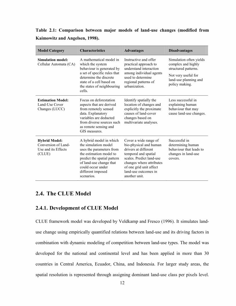
TABLE 2.1: COMPARISON BETWEEN MAJOR MODELS OF LAND-USE CHANGES (MODIFIED FROM KAIMOWITZ AND

ANGELSEN, 1998). ...................................................................................................................................... 12

TABLE 3.1: EXAMPLE OF A CONVERSION MATRIX IN TABLE FORMAT. .................................................................. 30

TABLE 3.2: EXAMPLE OF A DEMAND FILE CREATED IN EXCEL. ............................................................................. 31

TABLE 4.1: METHODS APPLIED TO MEASURE THE ASSOCIATION BETWEEN DIFFERENT PAIRS OF GIS LAYERS

(ADAPTED FROM BONHAM-CARTER, 1994). ................................................................................................ 40

TABLE 5.1: AVAILABLE LAND-USE MAPS OF THE SN WATERSHED (ADAPTED FROM SEIDOU AND LAPEN, 2010). . 49

TABLE 5.2: SURFACES OF LAND-USE CLASSES FOR TIME SERIES: 1991, 1995, 1998, 2000, AND 2005. .................. 58

TABLE 5.3: DEMAND IN SURFACES OF LAND-USE CLASSES STARTING FROM 1991 TO 2020. ................................. 59

TABLE 5.4: LAND-USE CONVERSION MATRIX. ...................................................................................................... 61

TABLE 5.5: LIST OF EXPECTED DRIVING FACTORS BEHIND LAND-USE CHANGES IN THE SN WATERSHED (ADAPTED

FROM SEIDOU AND LAPEN, 2010). .............................................................................................................. 64

TABLE 5.6: CALCULATED BETA COEFFICIENTS AND ROC VALUES OF BINARY LOGISTIC REGRESSION FOR LAND-

USE CLASSES OF 1991 IN SPSS. ................................................................................................................... 67

TABLE 5.7: ACCURACY RESULTS OF SIMULATED AND REALITY MAPS OF 1998 OBTAINED FROM SCENARIO 1....... 76

TABLE 5.8: ACCURACY RESULTS OF SIMULATED AND REALITY MAPS OF 2005 OBTAINED FROM SCENARIO 1....... 76

TABLE 5.9: ACCURACY RESULTS OF MAP OF 1991 AND SIMULATED MAP OF 2005 OBTAINED FROM SCENARIO 2. 78

TABLE 5.10: ACCURACY RESULTS OF MAP OF 1991 AND SIMULATED MAP OF 2020 OBTAINED FROM SCENARIO 2.

................................................................................................................................................................... 78

TABLE 5.11: ACCURACY RESULTS OF SIMULATED AND REALITY MAPS OF 1998 OBTAINED FROM SCENARIO 3..... 80

TABLE 5.12: ACCURACY RESULTS OF SIMULATED AND REALITY MAPS OF 2005 OBTAINED FROM SCENARIO 3..... 80

xi

LIST OF ABBREVIATIONS

AnnAGNPS Annualized Agricultural Non-Point Source

BLR Binary Logistic Regression

CLUE-S Conversion of Land-Use and its Effects at Small regional Extent

Dyna-CLUE Dynamic Conversion of Land-Use and its Effects

FPF False Positive Fraction

GIS Geographic Information System

ROC Relative Operating Characteristic

SN South Nation

SNC South Nation Conservation

SPSS Statistical Package for the Social Sciences

TPF True Positive Fraction

1

CHAPTER 1

INTRODUCTION

1.1. Background

Land cover is the layer of soil and biomass including natural vegetation, crops, and

infrastructures that cover the land surface. Land-use is the means through which humans

exploit the land cover (Verburg et al., 2000). Land-use change is the modification in the

purpose of the land cover, which is not only the change in land cover, but also changes in

management. Change detection is a process of identifying and analyzing the differences of a

phenomenon through monitoring at different times. The detection and analysis of changes in

multi-temporal remote-sensing data have achieved remarkable success in several application

domains (Soepboer, 2001).

In the last three decades, the South Nation (SN) watershed has accomplished an outstanding

economic growth, which was reflected in an increase in the urban areas and decrease in the

rural areas. This urbanisation expansion resulted in continuous conversion of some

agricultural land-uses to urban uses including residential, industrial and infrastructure

projects (SNC, 2006). Consequently, many questions arise such as; how does this process

occur? Which type of land-use is more likely to be replaced by urban? Where and how fast

does that urbanisation expansion occur? Which driving factors are behind such process?

Modeling can be employed to answer these questions and also to predict land-use

conversions. Several types of models have been developed, however most of them are at the

descriptive level rather than at the predictive level (Tian et al., 1993).

2

1.2. Types of Models

Mulligan and Wainwright (2004) classified models into two major types: physical (or

hardware) and mathematical models. Physical models are scaled-down versions of real-world

situations that are used when mathematical models would be complex, uncertain and/or

inapplicable due to lack of knowledge. Several mathematical models simulate land-use

changes based on human activities and socio-economic drivers. The most known ones are

Conversion of Land-Use and its Effects (CLUE) (Veldkamp and Fresco, 1996), Cellular

Automata (CA) (White et al., 1997), and Land-Use Cover Changes (LUCC) (Lambin and

Geist, 2002).

1.3. Research Problem and Objectives

Land-covers have major effects on natural resources, productivity and rural living conditions

which directly influence our lives through the changes of the landscape and living

environment (Palang et al., 2000). Those changes are often caused by socio-economic

driving factors (Riebsame et al., 1994). The study area (South Nation watershed) had

undergone significant land-use changes during the last three decades (SNC, 2006). It is

necessary to investigate the changes in land-use pattern to have better understanding of this

process. Spatial simulation of land-use changes is very important to determine and quantify

the interaction between land-use dynamic changes and potential drivers causing changes in

the area under investigation. In this research work, we will investigate the following points:

The evolution of land-use in the SN watershed in the near and far future.

The most significant driving factors behind land-use changes in the SN watershed.

The impact of land-use restriction policy on the conversions of land-use covers.

3

1.4. Specific Research Objective

The specific objective of this research work is to generate future land-use maps of the SN

watershed which can serve in the future as input data in the AnnAGNPS (Annualized

Agricultural Non-Point Source) model (Bingner et al., 2007). From the land-use modeling

software available in the literature, the dynamic version of CLUE model, known as Dyna-

CLUE, was selected to model the land-use changes in the SN watershed, for the following

reasons:

Dyna-CLUE is a hybrid model that combines estimation and simulation models, which

uses the parameters from the estimation model to predict the spatial pattern of land-use

changes that could occur under different conditional scenarios;

Dyna-CLUE is an empirical model that aims to quantify the relationships between

variables using empirical data and statistical methods;

Dyna-CLUE is a multi-scale land-use change model developed for understanding and

predicting the impact of bio-physical and socio-economic forces that drive land-use

changes;

The model projects and displays cartographically the future land-use patterns that result

from the continuation of current land-use or actual land-cover map;

The model can simulate and locate 'hot-spots' of land-use changes at fine local scale of

spatial resolution; and

The modeling outcome of Dyna-CLUE can be used by land-use planners to make

decisions about the land-use planning desired for the future.

4

Dyna-CLUE has been successfully used in several case studies with a local to regional

extent and at resolution ranging from 20 to 1000 meters (Veldkamp and Fresco, 1996;

Verburg et al., 2002; Verburg and Veldkamp, 2003).

1.5. Methodology

This study aims to combine remote sensing Geographic Information System (GIS), and

Dyna-CLUE spatial simulation modeling approach to detect changes in land-use pattern of

the SN watershed throughout a period of 30 years (1990-2020). The model has been applied

based on resolution of 250 meter data in which each pixel contains a single land-use class.

The model helps to visualize future land-use scenarios with different hypotheses of the SN

watershed. Demographic and socio-economic drivers were integrated to study their impacts

on the changing process of land-use patterns. The methodology through which the Dyna-

CLUE model was applied needs to consider the following four parts:

(1) Land-use requirements: they represent the land-use demands in the surfaces of each

land-use class available in the study area. These requirements are calculated outside the

Dyna-CLUE model using Microsoft Excel.

(2) Location characteristics and suitability: in Dyna-CLUE model, the location suitability is

a major determinant of the competitive capacity among land-use classes at a specific

location, and it is based on empirical analysis of preferences between land-use classes

and potential driving factors. In the present study, the stepwise method in the logistic

regression analysis is used in the Statistical Package for the Social Sciences (SPSS)

software to indicate the probability of a certain cell to be devoted to a land-use class

given a set of potential driving factors.

5

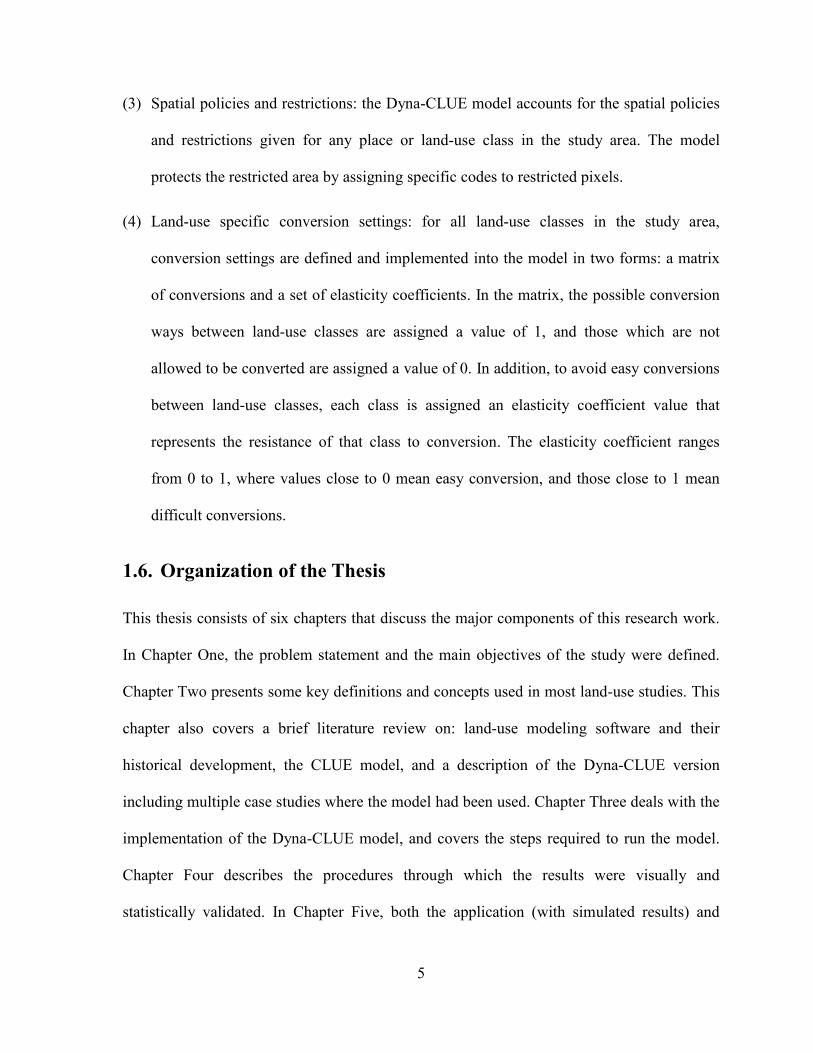
(3) Spatial policies and restrictions: the Dyna-CLUE model accounts for the spatial policies

and restrictions given for any place or land-use class in the study area. The model

protects the restricted area by assigning specific codes to restricted pixels.

(4) Land-use specific conversion settings: for all land-use classes in the study area,

conversion settings are defined and implemented into the model in two forms: a matrix

of conversions and a set of elasticity coefficients. In the matrix, the possible conversion

ways between land-use classes are assigned a value of 1, and those which are not

allowed to be converted are assigned a value of 0. In addition, to avoid easy conversions

between land-use classes, each class is assigned an elasticity coefficient value that

represents the resistance of that class to conversion. The elasticity coefficient ranges

from 0 to 1, where values close to 0 mean easy conversion, and those close to 1 mean

difficult conversions.

1.6. Organization of the Thesis

This thesis consists of six chapters that discuss the major components of this research work.

In Chapter One, the problem statement and the main objectives of the study were defined.

Chapter Two presents some key definitions and concepts used in most land-use studies. This

chapter also covers a brief literature review on: land-use modeling software and their

historical development, the CLUE model, and a description of the Dyna-CLUE version

including multiple case studies where the model had been used. Chapter Three deals with the

implementation of the Dyna-CLUE model, and covers the steps required to run the model.

Chapter Four describes the procedures through which the results were visually and

statistically validated. In Chapter Five, both the application (with simulated results) and

6

validation (with real land-use maps) of the developed model are presented. Additionally, the

essential driving factors behind land-use changes in the SN watershed are identified based on

the results of the logistic regression models. Chapter Six covers the discussion of the results

as well as the conclusions, contributions, and suggestions proposed for future research.

7

CHAPTER 2

LITERATURE REVIEW

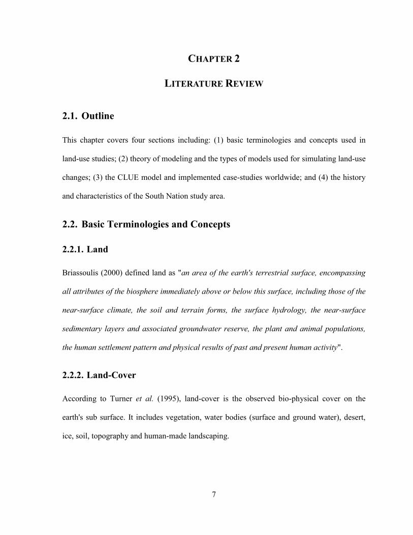
2.1. Outline

This chapter covers four sections including: (1) basic terminologies and concepts used in

land-use studies; (2) theory of modeling and the types of models used for simulating land-use

changes; (3) the CLUE model and implemented case-studies worldwide; and (4) the history

and characteristics of the South Nation study area.

2.2. Basic Terminologies and Concepts

2.2.1. Land

Briassoulis (2000) defined land as "an area of the earth's terrestrial surface, encompassing

all attributes of the biosphere immediately above or below this surface, including those of the

near-surface climate, the soil and terrain forms, the surface hydrology, the near-surface

sedimentary layers and associated groundwater reserve, the plant and animal populations,

the human settlement pattern and physical results of past and present human activity".

2.2.2. Land-Cover

According to Turner et al. (1995), land-cover is the observed bio-physical cover on the

earth's sub surface. It includes vegetation, water bodies (surface and ground water), desert,

ice, soil, topography and human-made landscaping.

8

2.2.3. Land-Use

Di Gregorio (2005) defined land-use as "the intended management activities underlying

human exploitation of a land-cover including any arrangements of a certain land-cover to

produce, change, or maintain it".

2.2.4. The Concept of Land-Use Change

Carter (1981) described the concept of land-use change as a "wide mix of land-uses where

changes among land-uses are subject to many variations driven by a complex set of socio-

economic drivers". Alternatively, Verburg et al., (2002) defined the concept of land-use

change as "a complex and dynamic model which is not only the conversion from non urban

land to urban land, but also the existence of competition between the drivers".

2.2.5. The Concept of Driving Factor

Van den Berg (1984) described the concept of driving factor as the influence of one or more

centrifugal or centripetal forces. Accordingly, he categorized the driving factors to two

classifications: centrifugal driving forces (drive for outside the area) and centripetal driving

forces (drive for inside the area). For example, in any study area, the pressure coming from

any activity related to ruralisation (gardening, landscaping, horticulture, horse-riding schools,

etc) is called centripetal driving force. On the opposite side, some urban land-users (or

owners) who are not able to operate in central locations (for example, in the urban zones) are

forced to leave their locations towards other more tolerable ones (rural zones) due to

centrifugal drivers such as noisy, smelly or dangerous industries. In both classifications

(centrifugal or centripetal driven forces), two main categories of driving factors are

distinguished: the bio-physical and the socio-economic drivers. The bio-physical drivers are

9

related to the occurrence of natural environment such as weather conditions, climate

variations, topography, volcanic eruptions, soil types, and drainage patterns. The socio-

economic drivers are related to demographic, social, economic, political and institutional

factors such as population density, industrial structure and change, technology and

technological change, the family, the market, and policies (Turner et al., 1995).

2.3. Theory of Modeling

The definition of modeling had confused researchers for a long time, until 1972 when

Meadows et al. defined it as follows: "modeling has one purpose which lies in the need of

communication. In another way, modeling can help people to communicate with each other

more easily". Models allow us to understand the complexity of the world, to reduce

uncertainty, and to update our knowledge and orient our vision towards the occurrence

possibility of simulated scenarios (Benders, 1996). Models can provide the user with

important assistance for present and future decision-making. In addition, modeling works as

experimental labs where different types of experiments and proposed theoretical hypotheses

could be tested and evaluated (Cheng, 2003).

2.3.1. Modeling Land-Use Changes

Models in land-use changes are used to improve our understanding of the dynamics of land-

use, and also to predict and evaluate various scenarios of activities (Brown et al., 2004).

Modeling land-use changes helps to resolve the following issues (Lambin, 2004):

Identification of the socio-economic and bio-physical drivers that cause land-use

changes.

10

Determination of the locations which are affected by land-use changes.

Determination of the temporal progress rate at which land-use and land-cover change.

2.3.2. Types of Models

Mulligan and Wainwright (2004) classified models into two major types: physical (or

hardware) and mathematical models. Physical models are scaled-down versions of real-world

situations, and are used when mathematical models are complex, uncertain and/or

inapplicable due to lack of knowledge. On the other hand, mathematical models are more

common and represent rates of change according to mathematical rules. This class of models

is divided into three types: empirical, conceptual and physical models. Empirical models

describe behaviour between variables on the basis of observations and relations between

variables with high predictive power but low explanatory depth. Conceptual models explain

the same concept but they describe the relationship between the variables. Physical models

are derived based on the above two types of models, are capable of producing more reliable

results.

In general, empirical models which use regression techniques are classified as non-spatial

models (which are also called multivariate statistical models), and spatial models (which

combines multivariate statistical models with GIS) (Lambin, 2004). The aim of spatial

empirical models is to quantify the relationships between variables using empirical data and

statistical methods, then project and display cartographically the future land-use patterns that

result from the projection of current land-use. This type of models is developed to describe

the relationship between the dependent variable (land-use class) and the independent

variables (driving factor) (Lambin et al., 2000).

11

2.3.3. Development of Land-Use Models

Most of the developed models were initially created to simulate urbanisation processes. In

the 1960s, models’ developers from the USA and Europe started to implement urban models

in combination with other discipline knowledge such as ecology, geography, mathematics,

regional science, economics, and many other disciplines. As a result, many larger socio-

economic models emerged during that period, such as the modeling projects of "Pittsburgh"

in Pennsylvania, and the model of "Peen-Jersey corridor" in San Francisco (Torrens, 2000).

Modeling researches conducted by Turner et al. (1995), Veldkamp and Fresco (1996);

Lambin et al. (2000), Verburg et al. (2002), and Verburg and Overmars (2007; 2009) had led

to the development of wide ranges of land-use models. Those new models were able to

explain and simulate spatial and non-spatial scenarios for deforestation and land-use

conversions from agriculture intensification to urbanisation.

2.3.4. Available Land-Use Models

Several land-use models were based on human activities and socio-economic drivers to

simulate land-use changes, including: Cellular Automata (CA) (White et al., 1997), Land-

Use Cover Changes (LUCC) (Lambin and Geist, 2002), and Conversion of Land-Use and its

Effects (CLUE) (Veldkamp and Fresco, 1996). Table 2.1 presents a brief overview and

assessment of each of the above models that are classified as simulation, estimation and

hybrid models, respectively.

12

Table 2.1: Comparison between major models of land-use changes (modified from

Kaimowitz and Angelsen, 1998).

Model Category Characteristics Advantages Disadvantages

Simulation model:

Cellular Automata (CA)

A mathematical model in

which the system

behaviour is generated by

a set of specific rules that

determine the discrete

state of a cell based on

the states of neighbouring

cells.

Instructive and offer

practical approach to

understand interaction

among individual agents

used to determine

regional patterns of

urbanization.

Simulation often yields

complex and highly

structured patterns.

Not very useful for

land-use planning and

policy making.

Estimation Model:

Land-Use Cover

Changes (LUCC)

Focus on deforestation

aspects that are derived

from remotely sensed

data. Explanatory

variables are deducted

from diverse sources such

as remote sensing and

GIS measures.

Identify spatially the

location of changes and

explicitly the proximate

causes of land-cover

changes based on

multivariate analyses.

Less successful in

explaining human

behaviour that may

cause land-use changes.

Hybrid Model:

Conversion of Land-

Use and its Effects

(CLUE)

A hybrid model in which

the simulation model

uses the parameters from

the estimation model to

predict the spatial pattern

of land-use change that

could occur under

different imposed

scenarios.

Cover a wide range of

bio-physical and human

drivers at different

temporal and spatial

scales. Predict land-use

changes where attributes

of one grid unit affect

land-use outcomes in

another unit.

Successful in

determining human

behaviour that leads to

changes in land-use

covers.

2.4. The CLUE Model

2.4.1. Development of CLUE Model

CLUE framework model was developed by Veldkamp and Fresco (1996). It simulates land-

use change using empirically quantified relations between land-use and its driving factors in

combination with dynamic modeling of competition between land-use types. The model was

developed for the national and continental level and has been applied in more than 30

countries in Central America, Ecuador, China, and Indonesia. For larger study areas, the

spatial resolution is represented through assigning dominant land-use class per pixels level.

13

For smaller study areas, the spatial resolution is usually based on homogeneous polygons or

even classified at the pixels level. The CLUE modeling approach was later modified by Peter

Verburg in collaboration with some colleagues at the Department of Environmental Sciences

at Wageningen University in The Netherlands, and the modified version was called CLUE-S

(Conversion of Land-Use and its Effects at Small regional extent) (Verburg et al., 2002).

Other versions were later developed in the same department; for example: Dyna-CLUE

(Verburg and Overmars, 2009) and CLUE-Scanner (Perez et al., 2010). CLUE’s versions are

freeware licensed programs that can be downloaded from the following link

http://www.ivm.vu.nl/CLUE. Appendix A provides a summary of the development and

structure of CLUE model and its versions.

2.4.2. CLUE Worldwide Case Studies

This section describes the performance of CLUE model (CLUE-S and Dyna-CLUE versions)

in eight case studies at different regions of the world. The model was applied to broad ranges

of land-use change scenarios including agricultural intensification, deforestation, land

abandonment, and urbanisation.

2.4.2.1. Sibuyan Island - Philippines 2001

Soepboer (2001) applied the CLUE-S modeling software to simulate land-use changes of the

Sibuyan Island located in the Philippines. The study area represented a total surface of

approximately 45,600 hectares where agricultural, mining, and residential activities were

localised in the coastal parts of the island. In addition, the area is characterised by steep

mountain slopes covered with forest canopy. The model was used to explore land-use

changes starting from 1997 to 2012 at a spatial resolution of 250×250 meter which means the

14

surface of one grid cell was fixed to 6.25 hectares. All analyses of geo-processing were made

on the Geographical Information System software platform ArcGIS 9.3. Thirteen driving

factors were used and classified under three categories: (1) geographic drivers (distance to

sea, road, city, and stream); (2) bio-physical drivers (diorite rock, ultramafic rock, sediments,

no erosion, moderate erosion, elevation, slope, and aspect); and (3) demographic driver

(mean population density). Binary logistic regression analysis was conducted on the

statistical software SPSS 13.0 using stepwise method. The performance of the resulting

regression models between land-use classes and expected driving factors were evaluated by

referring to the ROC method (Relative Operating Characteristic) applied by Pontius and

Schneider (2001). The results showed that the CLUE-S model had the potential to support

the decision-making in land-use planning and natural resource management. The model was

found to be very sensitive to small changes in the input of the demand module. Visual

comparison between simulated map and true map of the same year was used to decide which

simulations were the best.

2.4.2.2. Selangor River - Malaysia 2002

Engelsman (2002) applied the CLUE-S model to study the development of urbanisation in

the Selangor river basin located in Malaysia. The study area covered a total surface of

161,700 hectares with high population density and variable landscape diversification. The

objective was the prediction of land-use changes for 15 years, starting from 1999 to 2014. In

that study, 15 driving factors were considered: (1) nine bio-physical drivers (altitude, four

types of soil textures, and four types of suitability class soils); (2) four geographic drivers

(distances to road, river, centre of residence, and centre of forest); and (3) two demographic

drivers (population density, and agricultural labour forces). Binary logistic regression

15

analysis was conducted by using SPSS with the stepwise method, and the goodness of fit of

the logistic regression model was measured using the ROC method. The geo-processing

analyses were made on ArcGIS 9.3 using pixels of 750 ×750 meter as unit of observation.

Results showed that the CLUE-S model was able to perform different simulations based on

the range of realistic demands. The model was found sensitive to the use of different matrix

settings between land-use classes. However, the author did not perform any validation

approaches to assess the obtained results.

2.4.2.3. Achterhoek - The Netherlands 2007

Verburg and Overmars (2007) used the CLUE-S model to simulate land-use changes in the

Achterhoek region in the Netherlands. The study region covered a surface area of 42,000

hectares, where dairy farming was considered as the main land-use activity. The model was

used to compare between two scenarios; the first one described land-use changes without

spatial policies, whereas in the second one, ecological spatial policies were applied to

preserve part of the landscaping area. The time horizon of the modeling process was from

2000 to 2018, and the spatial resolution was set to 50×50 meter. The driving factors used

were classified into two categories; (1) geographic (distances to highway, provincial road,

cities, and streams); and (2) bio-physical (slope, elevation, soil characteristics, and

groundwater level). The binary logistic regression analysis was performed using the stepwise

method. Researchers applied the ROC method to test the performance of the resulting

regression models between land-use classes and expected driving factors. Results showed

that the model was able to respond to designated policies and converted the dairy farming

and grazing activities to other potential locations, where the degree of biodiversity losses in

land degradation was less significant. Authors used visual observation between simulated

16

and true map of the same year to select the best output. They concluded that the CLUE-S

model could be a useful tool to assess, discuss, and adjust policies in land-use changes, and

they also recommended using the model in further comparable studies.

2.4.2.4. Taips County - China 2007

The CLUE-S model was used by Jinyan et al. (2007) to model land-use changes at the Taips

County in China. The study area covered a total surface of 341,500 hectares, where farming

and pasturing were considered as the main agricultural activities. Three categories of driving

factors were considered: (1) stable controlling drivers (elevation, degree of slope, aspect,

landform, and soil texture); (2) seasonal changing drivers (annual changes of air temperature,

and precipitation); and (3) socio-economic drivers. The spatial resolution used was 100×100

meter with a grid surface of 1 hectare. The binary logistic regression analysis was performed

using the stepwise method. The performance of the resulting regression models between

land-use classes and driving factors was evaluated using the ROC method. The results

demonstrated significant correlation between land-use changes and their driving factors, and

allowed the decision-maker to select the best sustainable development strategy for the Taips

County.

2.4.2.5. Pennsylvania County - USA 2009

Batisani and Yarnal (2009) applied the CLUE-S model to study the transition of agricultural

land to urban in the Pennsylvania County in the United States. The Pennsylvania County

covered an area of 288,700 hectares, and was rated as a retirement destination. Over the

years the number and size of farms had decreased as the number of rural non-farm residents

had increased in the county. The researchers considered a list of bio-physical factors such as

17

topography, soil suitability for agricultural production, and population density as the major

driving factors behind urbanisation of the county. The map analyses were made on ArcGIS

9.3 at spatial resolution of 100×100 meter, and the SPSS 13.0 was used to conduct the binary

logistic regression analysis. The performance of the resulting regression models was

evaluated via the ROC method, and the model was calibrated by adjusting its parameters.

Results showed that land-use changes in the county were dominated by transitions from

agricultural to urban land-use, and by exchanges in location between forest and others land-

use classes. Researchers proved that the model was able to simulate urban land-use changes

at the county level.

2.4.2.6. Northern Thailand - Thailand 2010

Trisurat et al. (2010) studied the deforestation activities in Northern Thailand using Dyna-

CLUE model. The study area extended over a total surface of approximately 17,300 hectares,

and consisted of flat forests in the lower north and mountainous forests in the west and upper

north of the region. The time horizon covered in this case study was between 2002 and 2050,

and the spatial resolution was set to 500×500 meter. The researchers considered 13 driving

factors which were classified into three main categories: (1) bio-physical drivers (annual

precipitation, soil texture, altitude, aspect, and slope); (2) geographic (distances to available

water body, main road, stream, river, village, and city); and (3) socio-economic drivers

(population density, and income). The simulated map for 2050 indicated that forests would

mainly persist in the west and upper north of the region, which is rocky and not easily

accessible. In contrast, the highest deforestation occurred in the lower north where flat areas

were impacted by commercial logging. Authors found that the model was very useful, not

only in simulating land-use allocation, but also in visualizing the landscape patterns of

18

remaining forests. Additionally, the model was able to identify the "hot zones" of

deforestation and important areas for biodiversity conservation. The authors recommended

adding more driving factors related to socio-economic variables as they noticed that this

category of drivers had the largest influence on deforestation.

2.4.2.7. Sangong Watershed - China 2010

Luo et al. (2010) applied the CLUE-S model to study the Sangong watershed in China. The

Sangong River drains the Tianshan Mountains into the southern Junggar Basin in Xinjiang

with a total catchment area of 167,000 hectares. The watershed consisted of six land-use

classes including farmland, woodland, grassland, residential, waters, and other lands. During

the past 50 years, land-use covers in the watershed had changed dramatically due to

reclamation, irrigation and cultivation, as well as the application of fertilizers across the

Sangong watershed (Luo et al., 2003). The time frame of the study extended from 2004 till

2030 with a spatial resolution of 50×50 meter. Researchers stated that demographic and

socio-economic drivers were behind land-use changes in the watershed, and considered the

population density, livestock density, water consumption, and crop production as main

driving factors behind land-use changes in the watershed. Results showed that the model was

able to allocate the land-use demand taking into consideration the effect of land-use

suitability and spatial policies. In addition, the model was able to highlight the location of the

"hot spot" which are the first areas were conversions might occur in the future. Researchers

concluded that the methodology adopted was able to simulate virtual cases of "What-If"

scenarios, which provided scientific support for land-use planning and management of the

watershed.

19

2.4.2.8. Pengyang County - China 2010

Zhu et al. (2010) applied the CLUE-S model to evaluate the implementation of the project

policy "Grain for Green Project" conducted by the Chinese government in the Pengyang

County. The project aimed to simulate the effects of the implementation of an ecological

agriculture policy between 1993 and 2005. The study area covered a surface of 252,900

hectares of mountains with forest, grassland, cropland, and others as main land-use classes,

and the resolution applied was set to 100×100 meter as unit of observation. Natural and

socio-economic driving factors such as slope, aspect, elevation, distance to road, soil types,

and population density were proposed as the main forces behind land-use changes in the

county. Results indicated that the model was capable of simulating the policy-dominated

areas.

2.4.2.9. Current Research

In previous case studies, CLUE’s versions (CLUE and Dyna-CLUE) were used to model the

process of land-use changes in eight case studies at different regions of the world. The spatial

units of observation applied ranged from 50 to 750 meter where each land-use class was

represented by one dominant pixel. Two categories of demographic and geographic driving

factors were used to highlight the probability of changes in land-use classes as a result of

those drivers. Inspired by the previous successful applications of the CLUE model to forecast

land-use changes, the present study apply this methodology to model land-use changes in the

South Nation watershed under the effect of various geographic and demographic driving

factors.

20

2.5. Study Area

2.5.1. Location

The South Nation (SN) watershed is located in Eastern Ontario between latitude 44°44´-

45°38´ North and longitude 75°32´- 74°22´ West (Figure 2.1). It covers an area of

approximately 400,000 hectares and includes 15 municipalities. The watershed is drained by

the South Nation River flowing North-East before joining the Ottawa River near Plantagenet.

Over its course, the South Nation River drops only 85 meters creating a flat landscape which

leads to poor drainage and consequently encourages the formation of several wetlands. The

SN watershed is under the authority of the South Nation Conservation (SNC) that is

governed by a board of directors made up of 13 representatives elected from across the

watershed. Together, the SNC, municipalities, government and individual landowners work

to maintain and improve the natural resources which consist one of the largest watershed in

Ontario (SNC, 2006).

http://www.nation.on.ca/pdf/

21

Figure 2.1: The South Nation watershed (adapted from SNC, 2006).

22

2.5.2. History

In the early 1800s, migration to the South-Eastern Ontario started due to the development in

logging, agricultural, and industrial activities (Diogo and Jeena, 1995). As the demand for

lumber grew in Britain, USA, and locally (to supply demands of new settlements), larger

areas of land in the SN watershed were deforested and commercial lumbering operations

were established throughout the entire area. Steamboats travelled the South Nation River to

backup the trade taking place on both sides of the Ottawa River. Later in the 1850s, a

railroad network was built and used as a new transport chain for goods and woods access to

and from the region. Wheat was the first crop grown in the area until the 1840s when the

farmers were forced to diversify their farming practices into livestock husbandry and

dairying. During the early 1900s, more demands for milk and butter were needed, and

therefore farmers introduced new techniques to improve their production (Coyne, 2001). The

introduction of electricity in the 20th

century brought many changes to the SN watershed area

where power lines were constructed and electrical motors were introduced in farming

activities to increase production. As a result, farming activities became more efficient, and

the economies and agro-industrial activities in the area were significantly improved (Diogo

and Jeena, 1995). Deforestation and intensive farming practices were observed where forests

and wetland land-use classes had been converted into other land-use classes. Additionally,

the increased number of villages in the area had dramatically affected the natural character of

the SN watershed as well as the river itself, which had contributed to increased incidences of

spring flooding and summer drought. On the other hand, the effect of deforestation and

flooding had also caused mass erosion of topsoil into the river banks. Since the early

settlement of the SN watershed till today, these problems have remained and the area is still

23

subjected to wind and water erosion, summer droughts, and spring flooding. From the recent

natural occurrences affecting the watershed, the most severe ones include the ice storms in

1942 and 1998, and the two landslides that occurred in 1971 and 1993 which moved around

70 and 50 acres of land, respectively (Coyne, 2001).

2.5.3. Trends in Land-Use Covers

Historically, land-use covers in the SN watershed had faced dramatic changes, and

accordingly, some of the land-use classes had been converted. The changes in land-use

covers occurred periodically and could be related to many driving factors as follows:

Forest: in the early 1800s when the lumbering industry started, forests in the SN watershed

had suffered significant environmental degradation. By 1920, little original forest remained

in the area where agriculture became the main farming activity. Today, lumbering is carried

out using more sustainable forestry methods (Coyne, 2001).

Agriculture: in late 1800s, due to the exponential growth in population density and

consequent increase in demands for food, many wetlands were converted to farming

activities. In 1996 census, agricultural lands covered roughly 59% of the watershed, where

70% of the farming activity consisted of cropland (mainly wheat) (Coyne, 2001).

Wetlands: in 1800, the wetland areas in the SN watershed covered 47.6% of the total

surface, while they only covered 15.6% in 1982. The major cause of wetland losses within

the watershed was the conversion to agriculture farming activities. Today, the total area of

wetlands within the SN watershed is around 180 km2 (Coyne, 2001).

24

2.5.4. Current Land-Use Covers

The actual land-use covers in the SN watershed include 60% agricultural, 34% forest, and

6% mixed urban (SNC, 2006). Compared to the last 200 years, it can be clearly noticed that

those three main land-use covers had faced dramatic conversions which allowed for the

existence of other land-use covers (bare and urban).

2.5.5. Specific Characteristics

The SN watershed is characterised by a large diversity of rural and urban characteristics

described as follows:

Population: the population of the SN watershed is a complex between urban and rural

categories. It represents a model of people with different cultural and professional

backgrounds living in the same geographical area and sharing the same environmental

conditions. Over the last 20 years, due to the geographical location of the SN watershed

nearby the capital and surrounded by well developed network of highways, migration occurs

and new comers come to reside in the SN watershed where they are engaged in multiple

economic activities.

Social Characteristic: the local residents of the SN watershed spend most of their time

working in the fields at regular intervals determined by agricultural seasons and/or holidays.

Different socio-economic classes between residents can be distinguished compared to areas

between suburbs and countryside.

Economic Characteristic: among the agricultural activities in the SN watershed, cropping

vegetable contributes in developing the agro-industrial sector. As a result, the economic


25

structure in some areas of the SN watershed has evolved rapidly from rural to agro-industrial

activities (SNC, 2006).

2.5.6. Driving Factors

Based on the historical trends of land-use conversions that occurred in the SN watershed;

two major categories of driving factors could be distinguished:

Demographic Driving Factors: since it is under the authority of the South Nation

Conservation; the SN watershed is subject to different governmental policies and engineering

plans. Also, the variation in population density has been found to influence the spatial pattern

of land-use changes of the watershed.

Geographic Driving Factors: the existence of a well developed public transportation

system in the capital region had encouraged people to no longer prefer to live in the urban

centre (capital) where high levels of stress and pollution existed, and motivated them to

move towards rural areas. In parallel, the rapid development of high technology offered more

employment opportunities and accelerated the migration of farmers from the rural areas

towards urban centre. As a result, agricultural lands were abandoned and conversions of

agricultural lands towards other land-use classes were most likely to occur.


26

CHAPTER 3

PRINCIPLES OF LAND-USE SIMULATION USING DYNA-CLUE

3.1. Outline

This chapter describes the Dyna-CLUE model which is used in the present study to predict

land-use changes in the South Nation watershed. It covers three sections which are model

description, statistical analyses, and Dyna-CLUE model’s parameters.

3.2. Dyna-CLUE Model Description

3.2.1. Model Structure

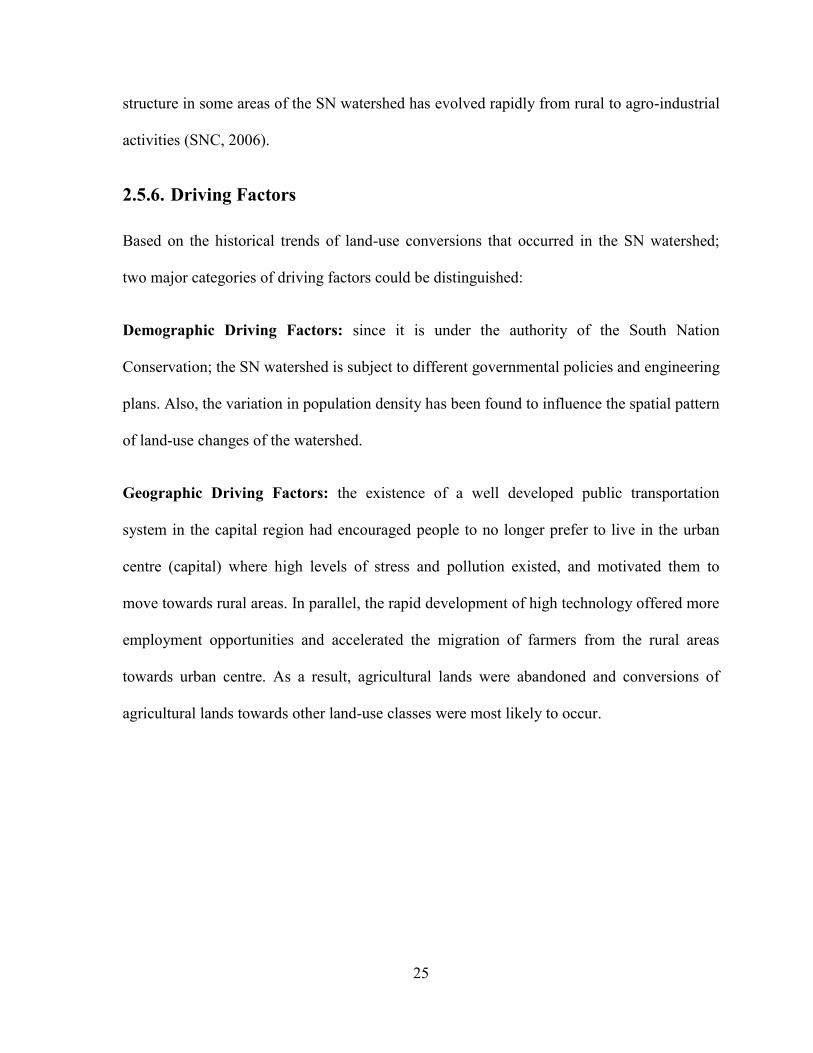
The Dyna-CLUE model (Dynamic Conversion of Land-Use and its Effects) is divided into

two levels: the non-spatial and the spatial analysis (Figure 3.1). The non-spatial analysis

calculates the area demands at the aggregate level, while the spatial analysis translates the

yearly demands into land-use changes at different locations within the time frame period of

the study area. Land-use is represented in a grid system where each pixel only contains one

land-use class. The structure of Dyna-CLUE model was developed with the objectives of:

Providing a clear view of the spatial variability of land-use changes under the effect

of driving factors;

Indicating the locations of "hot-spots" areas that may be converted under realistic

scenarios; and

Analysing the relationships between the driving factors and land-use covers in spatial

representation.

27

Figure 3.1: The structure of Dyna-CLUE model (adapted from Verburg and Overmars,

2009).

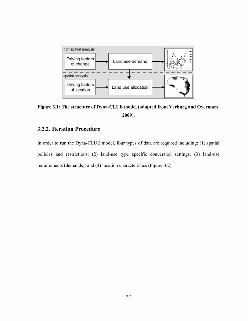
3.2.2. Iteration Procedure

In order to run the Dyna-CLUE model, four types of data are required including: (1) spatial

policies and restrictions; (2) land-use type specific conversion settings; (3) land-use

requirements (demands); and (4) location characteristics (Figure 3.2).

28

Figure 3.2: Flow chart of the allocation procedure in Dyna-CLUE model (adapted from

Verburg and Overmars, 2009).

3.2.2.1. Spatial Policies and Restrictions

Restricted areas, shown in Figure 3.3, are specific pixels of land-use classes located in the

study area that are not allowed to be converted into any other class. Such restriction is

represented in Dyna-CLUE model with the following codes:

0 : code for active cells which are the only cells allowed to be converted;

-9999 : code for "No Data" value(s); and

-9998 : code for restricted area.

29

Figure 3.3: Maps of restricted areas (in black) in Dyna-CLUE model (adapted from

Verburg and Overmars, 2009).

Once created, grids of restricted areas should be converted into ASCII format and must be

saved under the code name "region_park1.fil" (Figure 3.4) in the same directory where the

model is installed (Verburg and Overmars, 2009).

Figure 3.4: Example of a restricted area in ASCII format for Dyna-CLUE model

(adapted from Verburg and Overmars, 2009).

30

3.2.2.2. Land-Use Type Specific Conversion Settings

Land-use type specific conversion settings is an A×A matrix where A equals the number of

land-use classes available in the study area. It determines the temporal dynamics of the

simulations, and indicates the sequences of possible and impossible conversions among land-

use classes. For example, in a case study of five land-use classes (forest, coconut, grassland,

rice fields, and others), the dimensions of the matrix will be 5×5 where rows and columns

represent the present and potential future land-use classes, respectively. If the conversion is

allowed, the value "1" is assigned to the corresponding cell, while if the conversion is not

allowed, the value "0" is used instead. This matrix (e.g. shown in Table 3.1) is first created in

Microsoft Excel, then converted to a text file and saved under the code name "allow.txt" in

the same directory where the model is installed.

Table 3.1: Example of a conversion matrix in table format.

3.2.2.3. Land-Use Requirements

Land-use requirements (demands) are time series of projected surfaces of land-use classes

available in the study area. The land-use demand could be calculated using several methods

such as the linear extrapolation of historical trends, and the socio-economic models. To

generate a land demand, the following steps must be conducted in the following order:

31

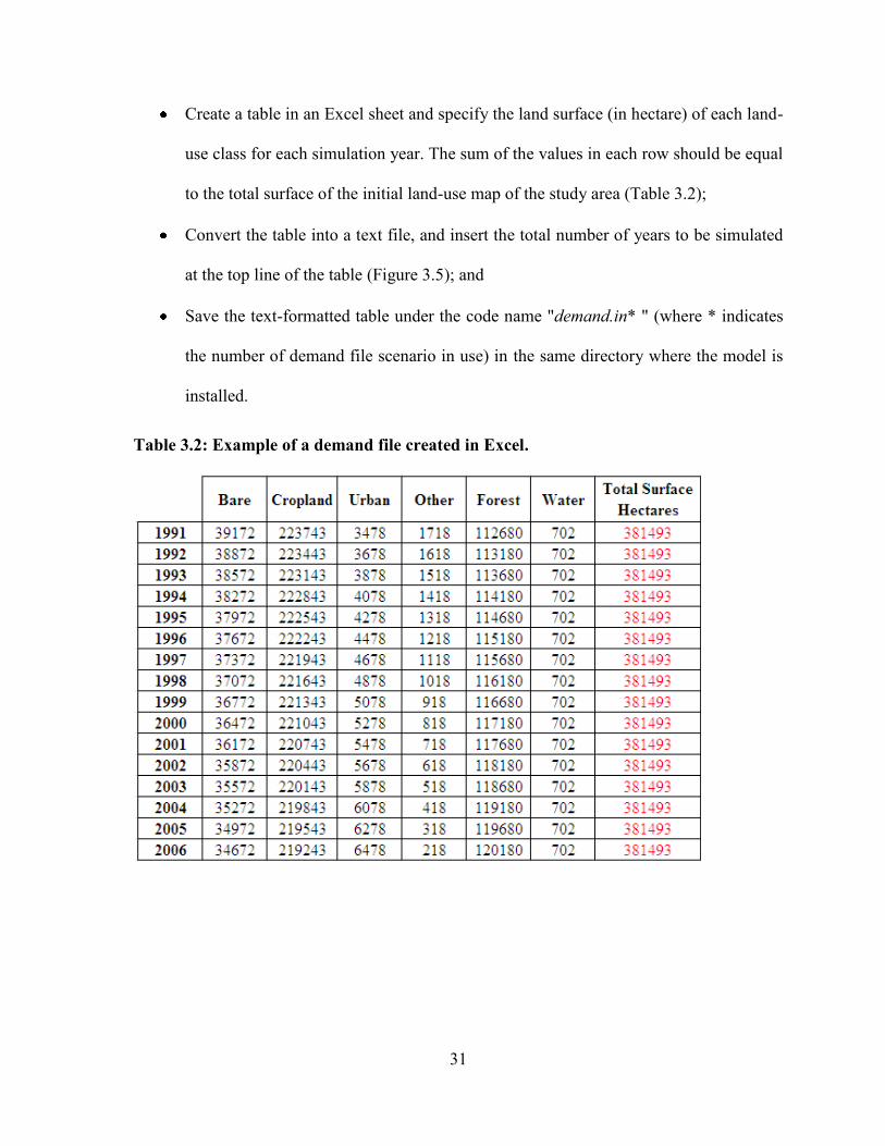
Create a table in an Excel sheet and specify the land surface (in hectare) of each land-

use class for each simulation year. The sum of the values in each row should be equal

to the total surface of the initial land-use map of the study area (Table 3.2);

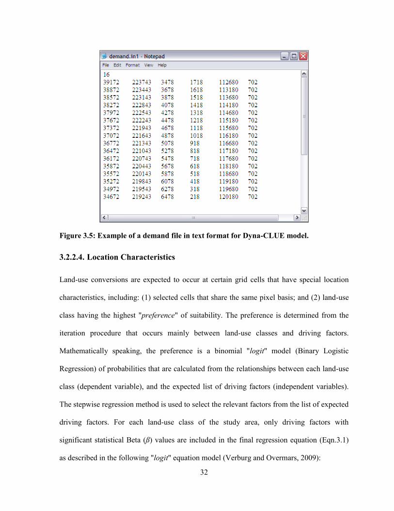
Convert the table into a text file, and insert the total number of years to be simulated

at the top line of the table (Figure 3.5); and

Save the text-formatted table under the code name "demand.in* " (where * indicates

the number of demand file scenario in use) in the same directory where the model is

installed.

Table 3.2: Example of a demand file created in Excel.

32

Figure 3.5: Example of a demand file in text format for Dyna-CLUE model.

3.2.2.4. Location Characteristics

Land-use conversions are expected to occur at certain grid cells that have special location

characteristics, including: (1) selected cells that share the same pixel basis; and (2) land-use

class having the highest "preference" of suitability. The preference is determined from the

iteration procedure that occurs mainly between land-use classes and driving factors.

Mathematically speaking, the preference is a binomial "logit" model (Binary Logistic

Regression) of probabilities that are calculated from the relationships between each land-use

class (dependent variable), and the expected list of driving factors (independent variables).

The stepwise regression method is used to select the relevant factors from the list of expected

driving factors. For each land-use class of the study area, only driving factors with

significant statistical Beta (ß) values are included in the final regression equation (Eqn.3.1)

as described in the following "logit" equation model (Verburg and Overmars, 2009):

33

(3.1)

Where:

Pi : probability of a grid cell to be allocated with a specific land-use class in a specific

location;

ß0 : constant obtained from the binary logistic regression model;

ßj : coefficients of driving factors estimated through the binary logistic regression

model; and

j,iX : the (thj ) location factor affecting the suitability of land-use (i).

The preparation of the "logit" models is conducted outside the Dyna-CLUE model using

certain statistical software (e.g. SPSS).

3.2.3. Allocation Procedure

Once the location preferences for each land-use class are calculated, the following allocation

steps are taken to assign the suitable land-use changes:

1. Determination of all grid cells that are allowed to change by excluding those which are

parts of protected areas.

2. For each grid cell (i), the total probability (TPROBi,u) is calculated for each of the

land-use class (u) according to the following equation:

(3.2)

Where:

Pi,u : the suitability of location (i) for land-use class (u) based on the "logit" model;

ELASu : the conversion elasticity for land-use (u); and

ITERu : an iteration parameter.

34

3. A preliminary allocation is made for all land-use classes by allocating the land-use

class with the highest total probability to the considered grid cell. This allocation

process will cause a certain number of grid cells to change land-use class. The total

allocated area of each land-use is then compared to the land-use demand areas

presented in the demand file. When the allocation predicted by the model is equal to

demand area required for each land-use class, the ultimate map of the year in question

is generated, and saved in the same directory where the model is installed. If not equal,

steps 2 and 3 are repeated until the demands are correctly allocated. After that, the

model continues to the next time step of its yearly simulation.

3.3. Statistical Analyses

3.3.1. Logistic Regression

Binary Logistic Regression (BLR) is a form of statistical regression that is used when the

dependent variable is dichotomous (0 or 1) and the independent variables are continuous or

categorical. For example, land-use classes are the dependent variables which could have a

value of 0 or 1 to indicate the absence or presence of a land-use class in a specific grid cell.

The BLR applies a maximum likelihood estimation to maximize the odds before

transforming the dependent variable into a "logit" variable. The odd of an event is defined as

the probability of the event occurring divided by the probability of the event not occurring.

The logistic regression equation with several independent variables is represented in the

following form:

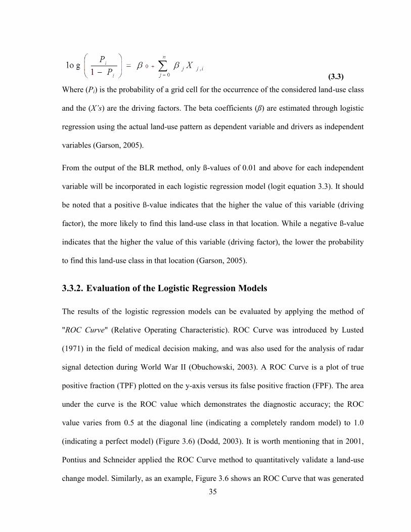
35

(3.3)

Where (Pi) is the probability of a grid cell for the occurrence of the considered land-use class

and the (X’s) are the driving factors. The beta coefficients (ß) are estimated through logistic

regression using the actual land-use pattern as dependent variable and drivers as independent

variables (Garson, 2005).

From the output of the BLR method, only ß-values of 0.01 and above for each independent

variable will be incorporated in each logistic regression model (logit equation 3.3). It should

be noted that a positive ß-value indicates that the higher the value of this variable (driving

factor), the more likely to find this land-use class in that location. While a negative ß-value

indicates that the higher the value of this variable (driving factor), the lower the probability

to find this land-use class in that location (Garson, 2005).

3.3.2. Evaluation of the Logistic Regression Models

The results of the logistic regression models can be evaluated by applying the method of

"ROC Curve" (Relative Operating Characteristic). ROC Curve was introduced by Lusted

(1971) in the field of medical decision making, and was also used for the analysis of radar

signal detection during World War II (Obuchowski, 2003). A ROC Curve is a plot of true

positive fraction (TPF) plotted on the y-axis versus its false positive fraction (FPF). The area

under the curve is the ROC value which demonstrates the diagnostic accuracy; the ROC

value varies from 0.5 at the diagonal line (indicating a completely random model) to 1.0

(indicating a perfect model) (Figure 3.6) (Dodd, 2003). It is worth mentioning that in 2001,

Pontius and Schneider applied the ROC Curve method to quantitatively validate a land-use

change model. Similarly, as an example, Figure 3.6 shows an ROC Curve that was generated

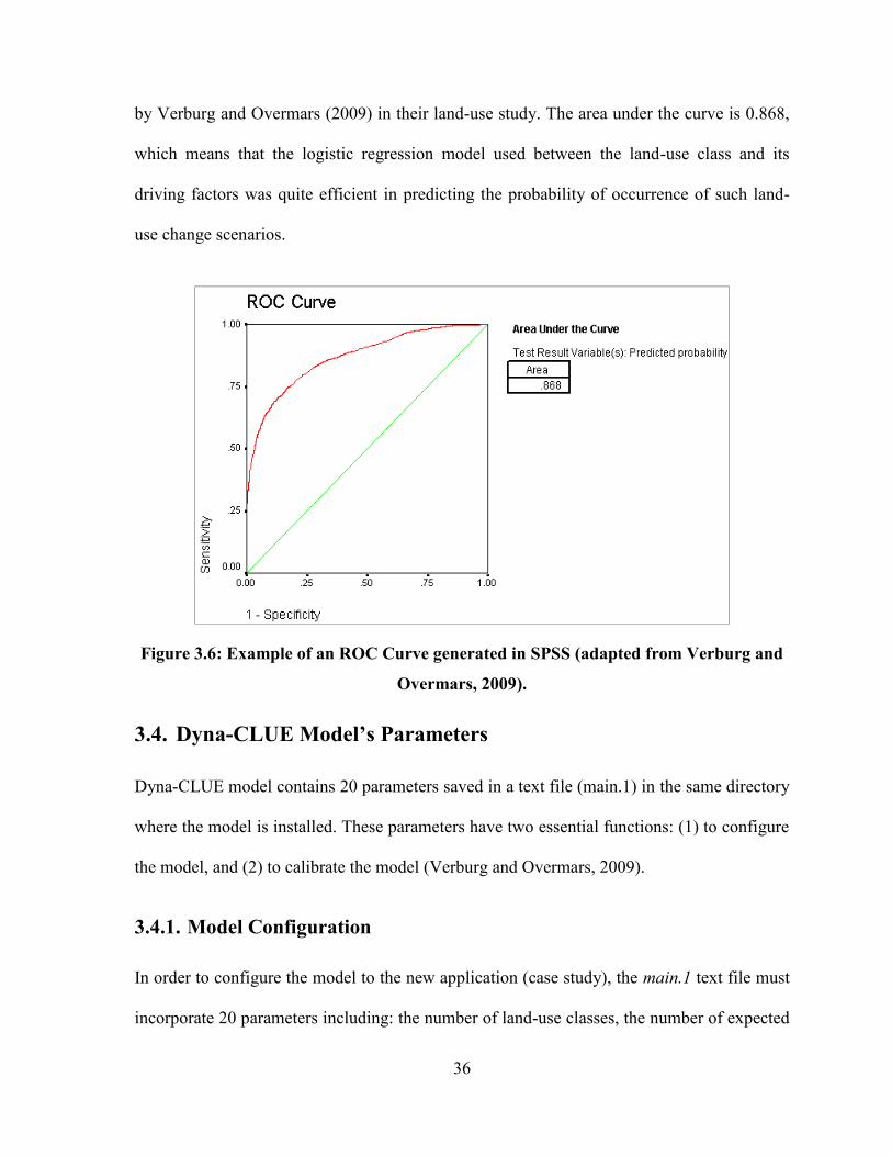
36

by Verburg and Overmars (2009) in their land-use study. The area under the curve is 0.868,

which means that the logistic regression model used between the land-use class and its

driving factors was quite efficient in predicting the probability of occurrence of such land-

use change scenarios.

Figure 3.6: Example of an ROC Curve generated in SPSS (adapted from Verburg and

Overmars, 2009).

3.4. Dyna-CLUE Model’s Parameters

Dyna-CLUE model contains 20 parameters saved in a text file (main.1) in the same directory

where the model is installed. These parameters have two essential functions: (1) to configure

the model, and (2) to calibrate the model (Verburg and Overmars, 2009).

3.4.1. Model Configuration

In order to configure the model to the new application (case study), the main.1 text file must

incorporate 20 parameters including: the number of land-use classes, the number of expected

37

and significant driving factors, the iteration variables, among others so as to represent the

area of study. Appendix B describes each of the 20 parameters required to configure the

model (Verburg and Overmars, 2009).

3.4.2. Model Calibration

Out of the 20 parameters, two parameters (initial land-use age of pixels, and elasticity

coefficients) are used to calibrate the model (Verburg and Overmars, 2009).

3.4.2.1. Initial land-Use Age of Pixels

An initial land-use age of pixels is a grid map of the study area that may be either randomly

generated by the model itself or created by the user. In that grid map, each pixel is assigned

with a certain value (before the beginning of simulations) that represents the period (in year)

that a specific class had been using this specific pixel location.

3.4.2.2. Elasticity Coefficients

Elasticity coefficients are values assigned by the user for land-use classes to indicate the

resistance of each class to the conversions. It is a scale that ranges from 0 (indicative of easy

conversion) to 1 (indicative of hard conversion, i.e., irreversible change). In other terms, the

closer the values to 0 the easier is the land-use conversion, and the closer the values to 1 the

harder is the land-use conversion.

The calibration of Dyna-CLUE model is performed by running the model several times using

an initial land-use age of pixels (either generated by the model or created by the user) with a

set of elasticity coefficients for land-use classes assigned by the user. The initial land-use age

of pixels and the elasticity coefficients of the simulation that gives the most reliable results

38

will be retained as the ones to be used in the final model. This calibration process is not

performed automatically by the model, and it mostly relies on the user’s judgement,

knowledge, and experience.

39

CHAPTER 4

VALIDATION OF RESULTS

4.1. Outline

This chapter demonstrates two types of validation techniques: statistical and visual

validation, both of which will be used to validate simulated maps obtained from the runs of

Dyna-CLUE model.

4.2. Concept of Validation

Simulation models are being increasingly used to solve problems and to aid in decision-

making. The developers and users of these models are concerned with whether a model and

its results are "correct", and this concern is addressed through model validation. Model

validation is defined as "proof that a computerized model within its domain of applicability

possesses a satisfactory range of accuracy consistent with the intended application of the

model" (Mulligan and Wainwright, 2004). The proof that a model is valid is generally

considered to be a process and is usually part of the total model development process.

4.3. Validation Techniques

This section introduces two validation techniques intended to be applied to judge on the

results obtained from the runs of Dyna-CLUE model. The model performance was assessed

by applying the following validation techniques:

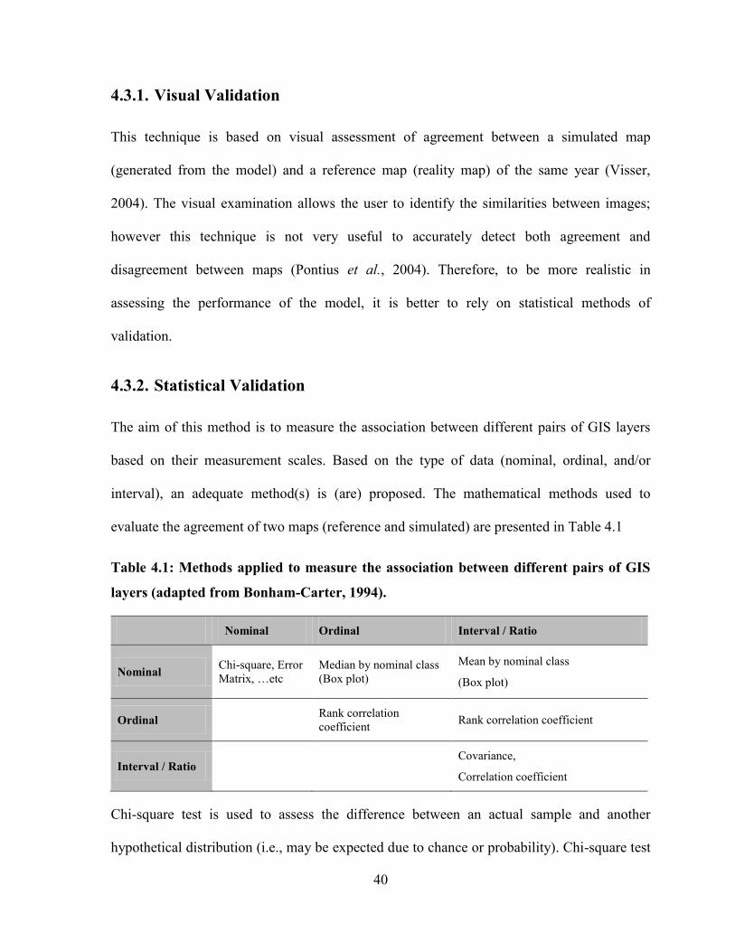
40

4.3.1. Visual Validation

This technique is based on visual assessment of agreement between a simulated map

(generated from the model) and a reference map (reality map) of the same year (Visser,

2004). The visual examination allows the user to identify the similarities between images;

however this technique is not very useful to accurately detect both agreement and

disagreement between maps (Pontius et al., 2004). Therefore, to be more realistic in

assessing the performance of the model, it is better to rely on statistical methods of

validation.

4.3.2. Statistical Validation

The aim of this method is to measure the association between different pairs of GIS layers

based on their measurement scales. Based on the type of data (nominal, ordinal, and/or

interval), an adequate method(s) is (are) proposed. The mathematical methods used to

evaluate the agreement of two maps (reference and simulated) are presented in Table 4.1

Table 4.1: Methods applied to measure the association between different pairs of GIS

layers (adapted from Bonham-Carter, 1994).

Nominal Ordinal Interval / Ratio

Nominal Chi-square, Error

Matrix, …etc

Median by nominal class

(Box plot)

Mean by nominal class

(Box plot)

Ordinal Rank correlation

coefficient Rank correlation coefficient

Interval / Ratio Covariance,

Correlation coefficient

Chi-square test is used to assess the difference between an actual sample and another

hypothetical distribution (i.e., may be expected due to chance or probability). Chi-square test

41

is usually easier to compute but it requires a large number of observations to ensure

convergence. Box plot is a way of graphically depicting groups of numerical data through

their five-number summaries: the smallest observation (sample minimum), lower quartile

(Q1), median (Q2), upper quartile (Q3), and largest observation (sample maximum). Box

plots display differences between populations without making any assumptions of the

underlying statistical distribution. Rank correlation coefficient measures the extent to which,

as one variable increases, the other variable tends to increase though not necessarily

according to a linear relationship. Rank correlation coefficient is commonly seen as an

alternative to Pearson's coefficient, which is used either to reduce the amount of calculation

or to make the coefficient less sensitive to non-normality in distributions. Covariance is a

measure of how much two random variables change together (i.e. if the variables tend to

show similar behavior). If the greater values of one variable mainly correspond with the

greater values of the other variable, and the same holds for the smaller values, and vice versa

for the opposite case. The sign of the covariance therefore shows the tendency in the linear

relationship between the variables. The correlation coefficient measures the covariation in

the magnitudes of two variables. However, this covariation is only to reflect on the

population (or universe) from which the observations were taken (Wasserman, 2004). In the

present study, the data generated by the Dyna-CLUE model includes maps in ASCII format,

which are considered nominal type of data (i.e., classes of land-uses). Therefore, based on

Table 4.1, the method which will be utilized to measure the association between pair of

nominal maps (simulated and reality maps) can be Chi-square and the error matrix. Further

information of the error matrix is illustrated below.

42

4.3.2.1. Mathematical Description of the Error Matrix

An error matrix is a square array of data classified in rows and columns representing the

number of sample units which could be pixels, clusters or polygons. Generally, the columns

represent the reference data (which can be generated from aerial photography, airborne

video, ground observation or ground measurement) while the rows represent the

classification of generated data (from model simulations). Each cell in the error matrix is

assigned a number based on the number of sample units assigned to a given land-use class in

the reference and generated data. The error matrix is an effective method to calculate

multiple accuracy parameters, such as: overall accuracy, producer’s accuracy, and user’s

accuracy of any nominal set of GIS pair of data (Congalton and Green, 1999).

4.3.2.2. Mathematical Representation of the Error Matrix

This section presents the error matrix in mathematical terms needed to perform the statistical

analyses in Chapter 5. Figure 4.1 shows the mathematical representation of an error matrix

where:

( ): total number of samples distributed into (k×k) matrix of cells where each sample is

assigned to one of:

(k) categories in the remotely sensed classification (rows of the matrix). In this case

study, (k) cells are generated from the Dyna-CLUE model; and

(k) categories in the reference data set (columns of the matrix). In this case study, (k)

cells are those cells in the reality maps.

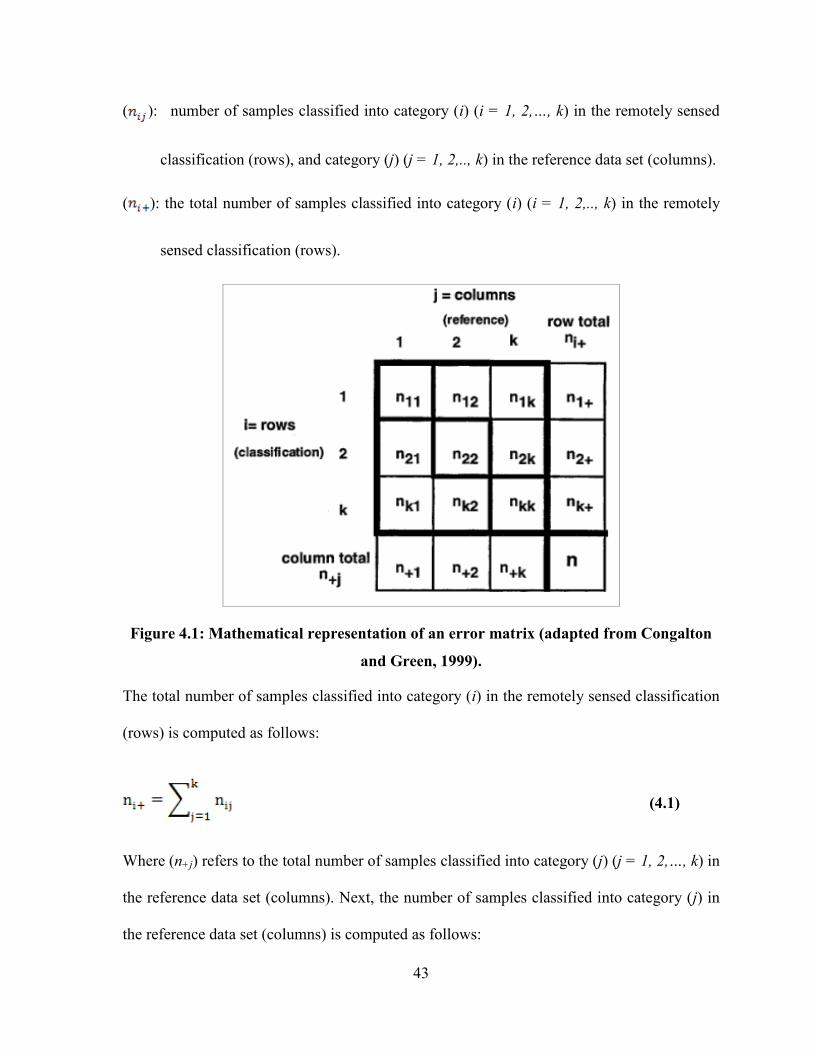
43

( ): number of samples classified into category (i) (i = 1, 2,…, k) in the remotely sensed

classification (rows), and category (j) (j = 1, 2,.., k) in the reference data set (columns).

( ): the total number of samples classified into category (i) (i = 1, 2,.., k) in the remotely

sensed classification (rows).

Figure 4.1: Mathematical representation of an error matrix (adapted from Congalton

and Green, 1999).

The total number of samples classified into category (i) in the remotely sensed classification

(rows) is computed as follows:

(4.1)

Where (n+j) refers to the total number of samples classified into category (j) (j = 1, 2,…, k) in

the reference data set (columns). Next, the number of samples classified into category (j) in

the reference data set (columns) is computed as follows:

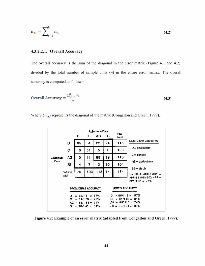
44

(4.2)

4.3.2.2.1. Overall Accuracy

The overall accuracy is the sum of the diagonal in the error matrix (Figure 4.1 and 4.2),

divided by the total number of sample units (n) in the entire error matrix. The overall

accuracy is computed as follows:

(4.3)

Where represents the diagonal of the matrix (Congalton and Green, 1999).

Figure 4.2: Example of an error matrix (adapted from Congalton and Green, 1999).

45

4.3.2.2.2. Producer’s Accuracy

The producer’s accuracy represents the individual category of accuracy instead of the overall

classification of accuracy. It is calculated by dividing the total number of correct sample

units (shared in the diagonal) by the total reference data. The producer’s accuracy is

computed as:

(4.4)

Where ) represents the total of shared correct samples in the diagonal , and (

represents the sum of total reference data of that specific class (column) (Congalton and

Green, 1999).

4.3.2.2.3. User’s Accuracy

Similar to the producer’s accuracy, the user’s accuracy represents the individual category of

accuracy instead of the overall classification of accuracy. It is calculated by dividing the total

number of correct pixels (shared in the diagonal) by the total number of classified pixels. The

user’s accuracy is computed as:

(4.5)

Where ) represents the total of shared correct samples in the diagonal , and

represents the sum of total classified data of that specific class (row) (Congalton and Green,

1999).

46

4.3.2.3. Interpretation of the Error Matrix

Larger value of the overall accuracy indicates that the two maps (reality map and simulated

map) are similar. Likewise, larger values of the producer’s accuracy and/or the user’s

accuracy are indicative of great spatial similarity among the pair of classes tested (in reality

map and simulated map). For example, Figure 4.2 shows an overall accuracy of 74%, which

means that, the generated and the reality maps (references) are similar. The accuracy of the

class "deciduous" is calculated by the producer accuracy for that specific class. This

calculation is performed by dividing the total number of correct sample units in the

deciduous category (i.e., 65) by the total number of deciduous sample units as indicated by

the reference data (i.e., 75); see Figure 4.2. This results in a good producer’s accuracy of

87% for the "deciduous" class. Additionally, the user’s accuracy of "deciduous" class is

computed by dividing the total number of correct pixels in the "deciduous" class (i.e., 65) by

the total number of pixels classified as deciduous (i.e., 115) which results in a value of 57%;

see Figure 4.2. In conclusion, 87% of the deciduous areas have been correctly identified as

"deciduous", and only 57% of the areas considered "deciduous" on the map are actually

deciduous on the ground (Congalton and Green, 1999).

47

CHAPTER 5

APPLICATION AND RESULTS

5.1. Outline

In this chapter all GIS data were brought together with the same spatial reference that

represents the location of the South Nation watershed (e.g., NAD_1983, UTM_Zone 18 N,

and D_North_American_1983). All analyses of geo-processing were made with ArcGIS 9.3

using pixels of 250 × 250 meter as unit of observation.

5.2. Methodology

Figure 5.1 illustrates the five main sections of the methodology applied. The first section

introduces and defines the implementation of different scenarios proposed to evaluate the

model performance. The second section presents the essential files required to run the model,

and also the results from the statistical analyses. The third section includes the

implementation of data files needed to run each scenario separately. The fourth section

presents the total number of simulated maps generated from the runs of the three scenarios.

Additionally, in this section simulated maps are sorted and grouped per scenario according to

their potential in testing the proposed hypotheses. The last section presents the statistical

methods used to validate results obtained in each scenario. Discussion on the results and on

the performance of the model is covered in Chapter 6.

48

Figure 5.1: Flowchart of the methodology used.

5.3. Scenarios Proposed

Three scenarios are prepared to simulate land-use changes of the SN watershed based on the

reality map of 1991.

Scenario 1 uses the linear trend calculated from year 1991 till 2020 with "no area

restriction" and with an "initial land-use age of pixels" generated by the model itself. The

purpose of this scenario is to assess the accuracy of the Dyna-CLUE model to generate maps

similar to reality.

Scenario 2 uses the same files as in scenario 1, but with an "area restriction" created by the

user on bare land-use class. The purpose of this scenario is to evaluate the performance of the

model in responding to applied policy.

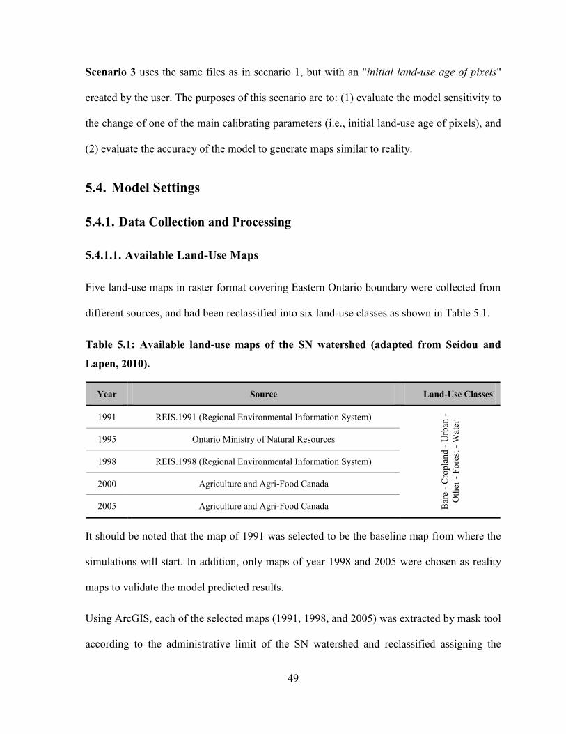
49

Scenario 3 uses the same files as in scenario 1, but with an "initial land-use age of pixels"

created by the user. The purposes of this scenario are to: (1) evaluate the model sensitivity to

the change of one of the main calibrating parameters (i.e., initial land-use age of pixels), and

(2) evaluate the accuracy of the model to generate maps similar to reality.

5.4. Model Settings

5.4.1. Data Collection and Processing

5.4.1.1. Available Land-Use Maps

Five land-use maps in raster format covering Eastern Ontario boundary were collected from

different sources, and had been reclassified into six land-use classes as shown in Table 5.1.

Table 5.1: Available land-use maps of the SN watershed (adapted from Seidou and

Lapen, 2010).

Year Source Land-Use Classes

1991 REIS.1991 (Regional Environmental Information System)

Bar

e -

Cro

pla

nd

- U

rban

-

Oth

er -

Fo

rest

- W

ater

1995 Ontario Ministry of Natural Resources

1998 REIS.1998 (Regional Environmental Information System)

2000 Agriculture and Agri-Food Canada

2005 Agriculture and Agri-Food Canada

It should be noted that the map of 1991 was selected to be the baseline map from where the

simulations will start. In addition, only maps of year 1998 and 2005 were chosen as reality

maps to validate the model predicted results.

Using ArcGIS, each of the selected maps (1991, 1998, and 2005) was extracted by mask tool

according to the administrative limit of the SN watershed and reclassified assigning the

50

codes 0, 1, 2, 3, 4, and 5 to bare, cropland, urban, other, forest, and water, respectively

(Figures 5.2, 5.3, and 5.4, respectively). Each of the reclassified rasters was then converted

into ASCII format as required by the Dyna-CLUE model. During the conversion, the code

"cov_all.0" (shown in Figure 5.5) is assigned to the output ASCII file of year 1991. To

document the applied procedures and repeatability, the procedures of "Extraction by Mask",

"Reclassification", and "Conversion Raster to ASCII" are programmed in the model builder

(Figure 5.5).

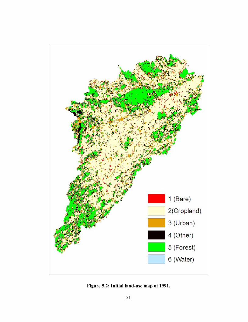
51

Figure 5.2: Initial land-use map of 1991.

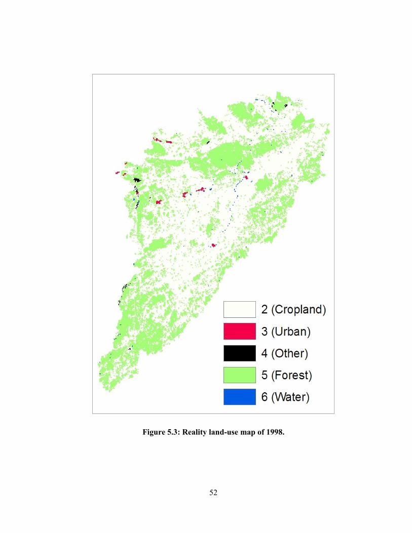
52

Figure 5.3: Reality land-use map of 1998.

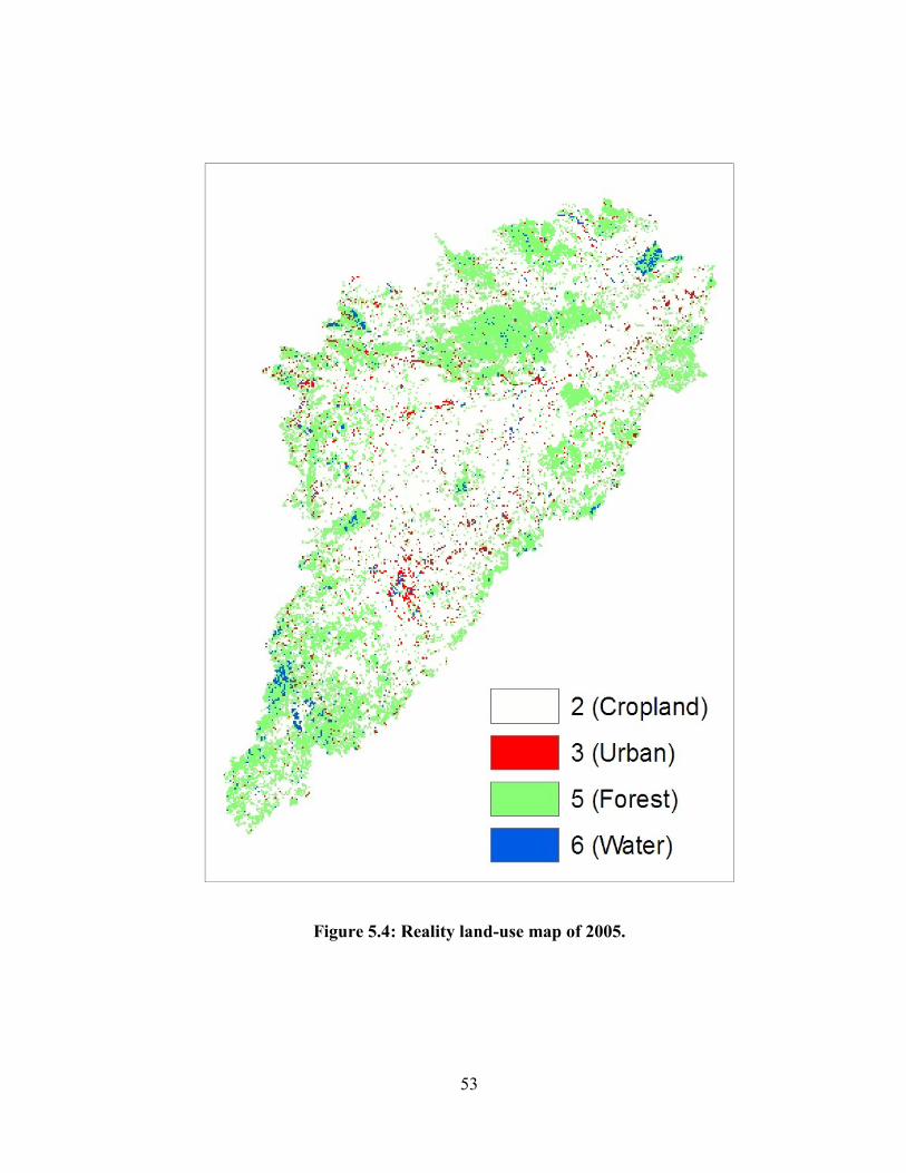
53

Figure 5.4: Reality land-use map of 2005.

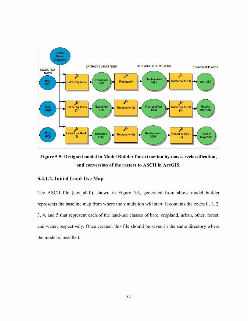
54

Figure 5.5: Designed model in Model Builder for extraction by mask, reclassification,

and conversion of the rasters to ASCII in ArcGIS.

5.4.1.2. Initial Land-Use Map

The ASCII file (cov_all.0), shown in Figure 5.6, generated from above model builder

represents the baseline map from where the simulation will start. It contains the codes 0, 1, 2,

3, 4, and 5 that represent each of the land-use classes of bare, cropland, urban, other, forest,

and water, respectively. Once created, this file should be saved in the same directory where

the model is installed.

55

Figure 5.6: Initial land-use map in ASCII format for Dyna-CLUE model.

5.4.1.3. Maps of Individual Land-Use Classes

Maps of individual land-use classes as rasters must be extracted from the initial map of 1991.

Each raster contains the code of one of the six classes available in the initial land-use map.

The extraction is carried out using the tool "Extract by Attributes", and then the extracted

rasters are converted into ASCII format. During the conversion, the code names "cov1_0.0,

cov1_1.0, cov1_2.0, cov1_3.0, cov1_4.0, and cov1_5.0" are assigned to bare, cropland,

urban, other, forest, and water land-use classes, respectively (Figure 5.7). The model of

model builder shown in Figure 5.7 displays the steps followed starting from the extraction to

the conversion.

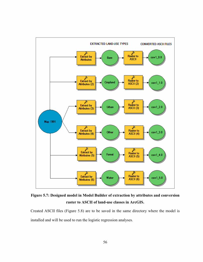
56

Figure 5.7: Designed model in Model Builder of extraction by attributes and conversion

raster to ASCII of land-use classes in ArcGIS.

Created ASCII files (Figure 5.8) are to be saved in the same directory where the model is

installed and will be used to run the logistic regression analyses.

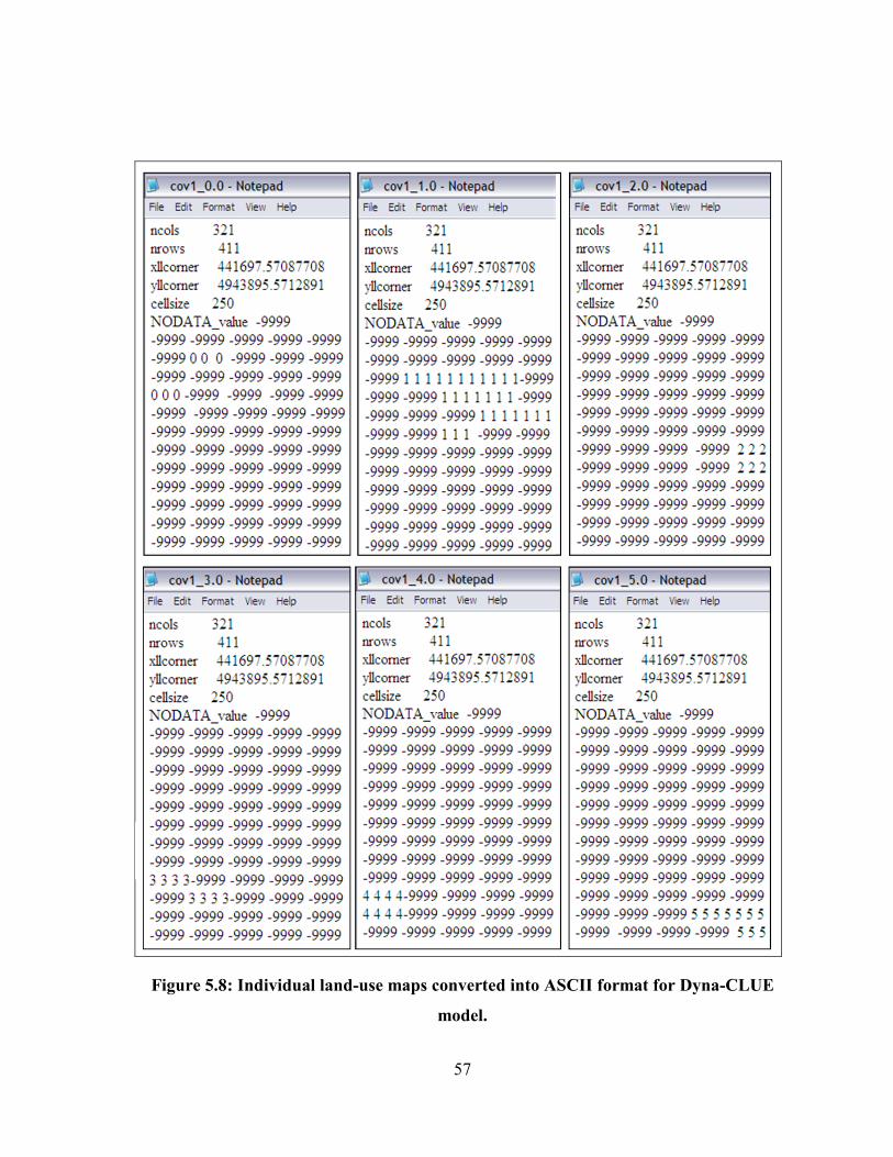
57

Figure 5.8: Individual land-use maps converted into ASCII format for Dyna-CLUE

model.

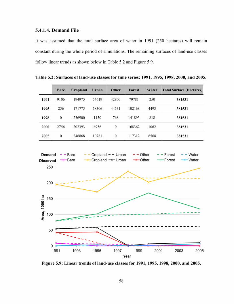
58

5.4.1.4. Demand File

It was assumed that the total surface area of water in 1991 (250 hectares) will remain

constant during the whole period of simulations. The remaining surfaces of land-use classes

follow linear trends as shown below in Table 5.2 and Figure 5.9.

Table 5.2: Surfaces of land-use classes for time series: 1991, 1995, 1998, 2000, and 2005.

Bare Cropland Urban Other Forest Water Total Surface (Hectares)

1991 9106 194975 54619 42800 79781 250 381531

1995 256 171775 58306 44531 102168 4493 381531

1998 0 236900 1150 768 141893 818 381531

2000 2756 202393 6956 0 168362 1062 381531

2005 0 246868 10781 0 117312 6568 381531

0

50

100

150

200

250

1991 1993 1995 1997 1999 2001 2003 2005

Are

a,

10

00

ha

Year

Bare Cropland Urban Other Forest Water


Demand

Observed

Figure 5.9: Linear trends of land-use classes for 1991, 1995, 1998, 2000, and 2005.

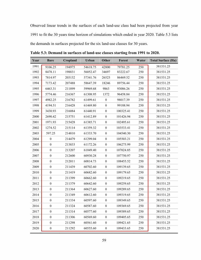
59

Observed linear trends in the surfaces of each land-use class had been projected from year

1991 to fit the 30 years time horizon of simulations which ended in year 2020. Table 5.3 lists

the demands in surfaces projected for the six land-use classes for 30 years.

Table 5.3: Demand in surfaces of land-use classes starting from 1991 to 2020.

Year Bare Cropland Urban Other Forest Water Total Surface (Ha)

1991 381531.25 9106.25 194975 54618.75 42800 79781.25 250

1992 8478.11 198831 56052.47 34697 83222.67 250 381531.25

1993 7814.97 203132 57341.76 26523 86469.52 250 381531.25

1994 7173.42 207488 58647.39 18246 89756.44 250 381531.25

1995 6463.31 211899 59969.68 9863 93086.26 250 381531.25

1996 5774.46 216367 61308.95 1372 96458.84 250 381531.25

1997 4982.25 216782 61499.61 0 98017.39 250 381531.25

1998 4194.51 216428 61469.80 0 99188.94 250 381531.25

1999 3430.93 216084 61440.91 0 100325.41 250 381531.25

2000 2690.42 215751 61412.89 0 101426.94 250 381531.25

2001 1971.93 215428 61385.71 0 102495.61 250 381531.25

2002 1274.52 215114 61359.32 0 103533.41 250 381531.25

2003 597.25 214810 61333.70 0 104540.30 250 381531.25

2004 0 214479 61299.04 0 105503.21 250 381531.25

2005 0 213833 61172.26 0 106275.99 250 381531.25

2006 0 213207 61049.40 0 107024.85 250 381531.25

2007 0 212600 60930.28 0 107750.97 250 381531.25

2008 0 212011 60814.73 0 108455.52 250 381531.25

2009 0 211439 60702.60 0 109139.65 250 381531.25

2010 0 211419 60682.60 0 109179.65 250 381531.25

2011 0 211399 60662.60 0 109219.65 250 381531.25

2012 0 211379 60642.60 0 109259.65 250 381531.25

2013 0 211364 60627.60 0 109289.65 250 381531.25

2014 0 211349 60612.60 0 109319.65 250 381531.25

2015 0 211334 60597.60 0 109349.65 250 381531.25

2016 0 211324 60587.60 0 109369.65 250 381531.25

2017 0 211314 60577.60 0 109389.65 250 381531.25

2018 0 211306 60569.60 0 109405.65 250 381531.25

2019 0 211298 60561.60 0 109421.65 250 381531.25

2020 0 211292 60555.60 0 109433.65 250 381531.25

60

Next, the highlighted red selection in Table 5.3 is copied to a text file, and saved under the

code name "demand.in1" in the same directory where the model is installed. It should be

noted that a line should be insert at the top of this file indicating the number of years of

simulations (30 years in this case study) (Figure 5.10).

Figure 5.10: Demand trend values for areas of land-use classes in text file format for

Dyna-CLUE model.

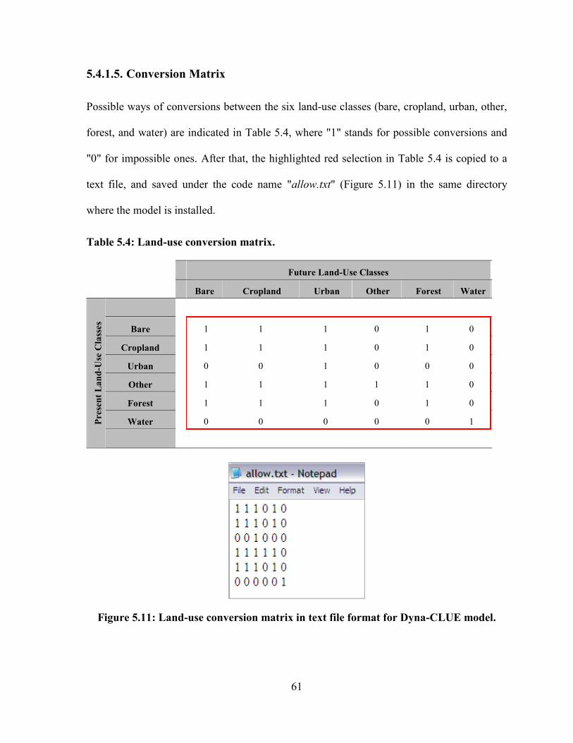
61

5.4.1.5. Conversion Matrix

Possible ways of conversions between the six land-use classes (bare, cropland, urban, other,

forest, and water) are indicated in Table 5.4, where "1" stands for possible conversions and

"0" for impossible ones. After that, the highlighted red selection in Table 5.4 is copied to a

text file, and saved under the code name "allow.txt" (Figure 5.11) in the same directory

where the model is installed.

Table 5.4: Land-use conversion matrix.

Future Land-Use Classes


Pre

sen

t L

an

d-U

se C

lass

es

Bare 1 1 1 0 1 0

Cropland 1 1 1 0 1 0

Urban 0 0 1 0 0 0

Other 1 1 1 1 1 0

Forest 1 1 1 0 1 0

Water 0 0 0 0 0 1

Figure 5.11: Land-use conversion matrix in text file format for Dyna-CLUE model.

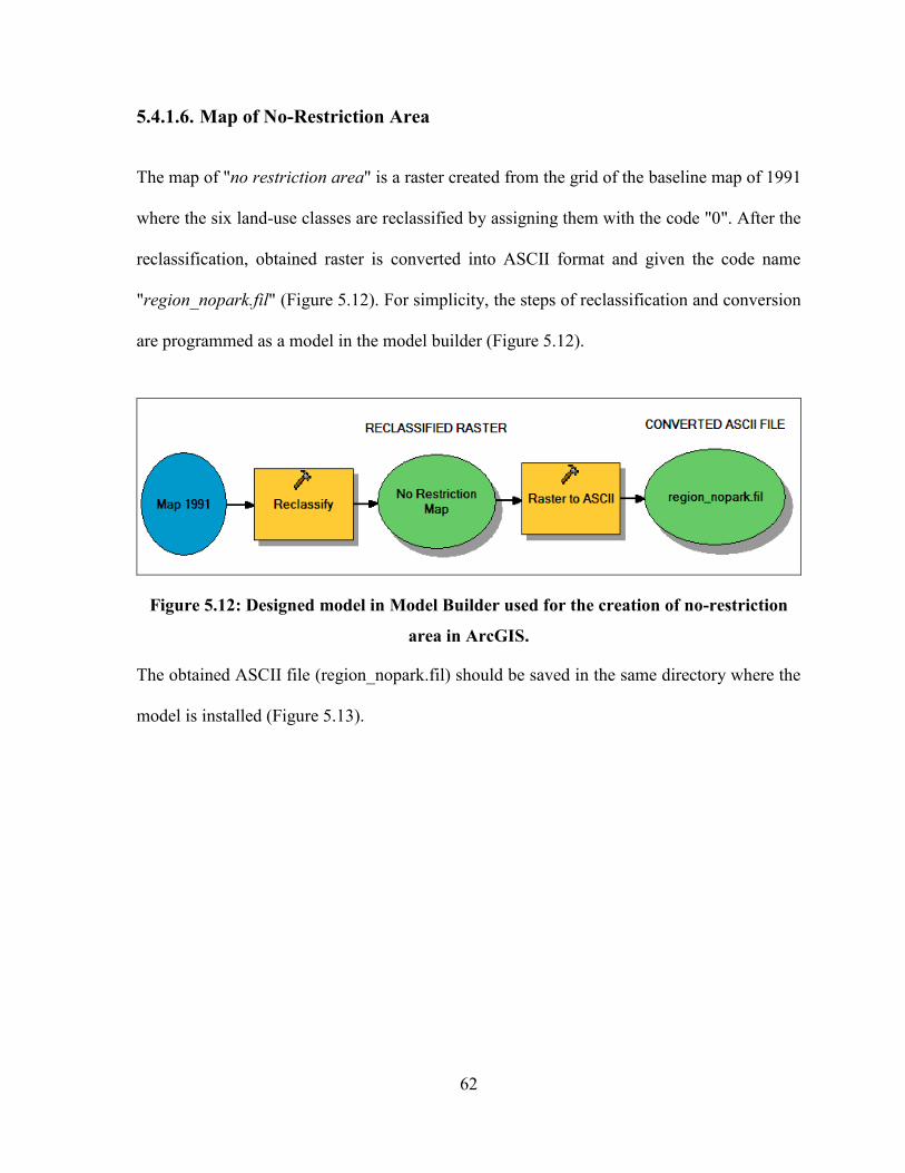
62

5.4.1.6. Map of No-Restriction Area

The map of "no restriction area" is a raster created from the grid of the baseline map of 1991

where the six land-use classes are reclassified by assigning them with the code "0". After the

reclassification, obtained raster is converted into ASCII format and given the code name

"region_nopark.fil" (Figure 5.12). For simplicity, the steps of reclassification and conversion

are programmed as a model in the model builder (Figure 5.12).

Figure 5.12: Designed model in Model Builder used for the creation of no-restriction

area in ArcGIS.

The obtained ASCII file (region_nopark.fil) should be saved in the same directory where the

model is installed (Figure 5.13).

63

Figure 5.13: No-restriction area in ASCII format for Dyna-CLUE model.

5.4.1.7. Expected Driving Factors

Seven maps of land-use drivers have been proposed as the expected forces behind land-use

changes in the SN watershed. These drivers were classified into two categories: geographic

and demographic as shown in Table 5.5.

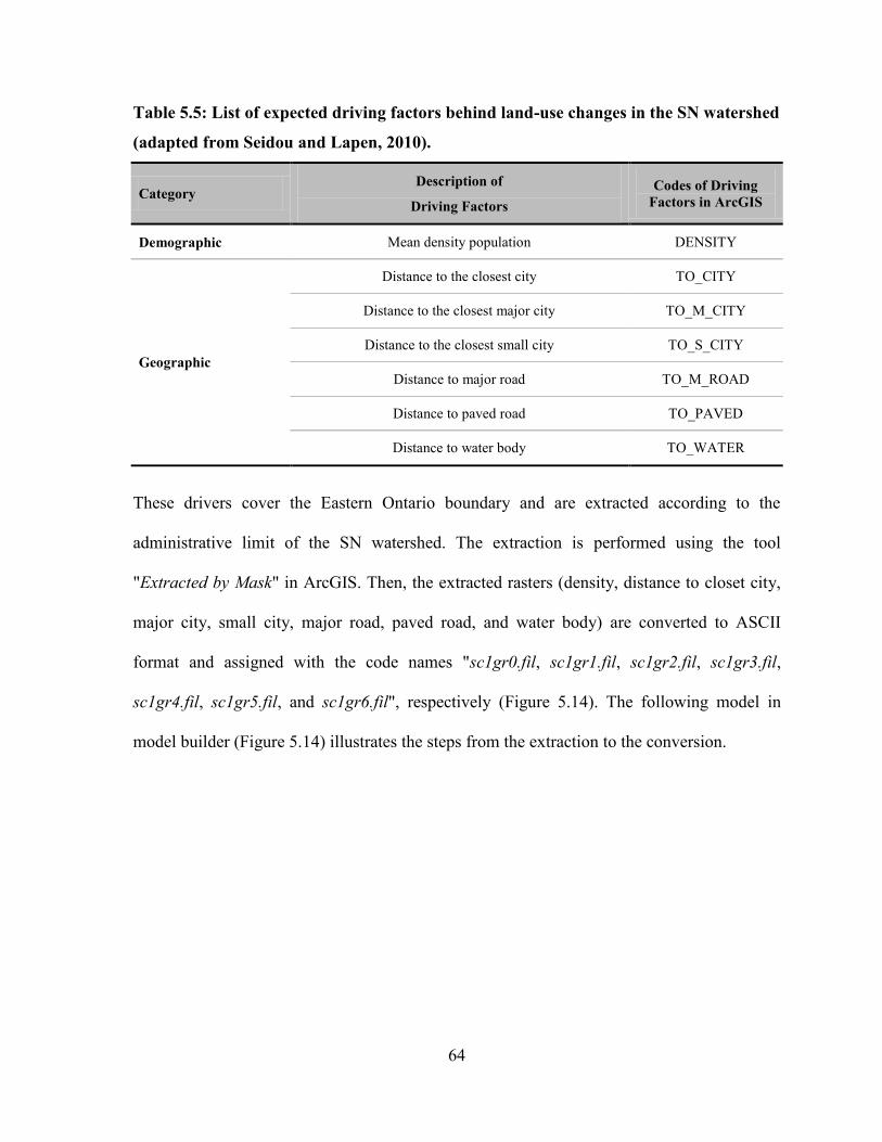
64

Table 5.5: List of expected driving factors behind land-use changes in the SN watershed

(adapted from Seidou and Lapen, 2010).

Category Description of

Driving Factors

Codes of Driving

Factors in ArcGIS

Demographic Mean density population DENSITY

Geographic

Distance to the closest city TO_CITY

Distance to the closest major city TO_M_CITY

Distance to the closest small city TO_S_CITY

Distance to major road TO_M_ROAD

Distance to paved road TO_PAVED

Distance to water body TO_WATER

These drivers cover the Eastern Ontario boundary and are extracted according to the

administrative limit of the SN watershed. The extraction is performed using the tool

"Extracted by Mask" in ArcGIS. Then, the extracted rasters (density, distance to closet city,

major city, small city, major road, paved road, and water body) are converted to ASCII

format and assigned with the code names "sc1gr0.fil, sc1gr1.fil, sc1gr2.fil, sc1gr3.fil,

sc1gr4.fil, sc1gr5.fil, and sc1gr6.fil", respectively (Figure 5.14). The following model in

model builder (Figure 5.14) illustrates the steps from the extraction to the conversion.

65

Figure 5.14: Designed model in Model Builder used to extract and convert expected

driving factors in ArcGIS.

Created ASCII files of driving factors (Figure 5.15) are saved in the same directory where

the model is located.

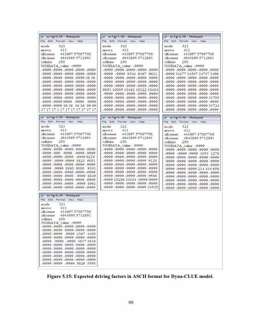
66

Figure 5.15: Expected driving factors in ASCII format for Dyna-CLUE model.

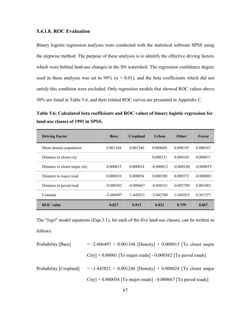
67

5.4.1.8. ROC Evaluation

Binary logistic regression analyses were conducted with the statistical software SPSS using

the stepwise method. The purpose of these analyses is to identify the effective driving factors

which were behind land-use changes in the SN watershed. The regression confidence degree

used in these analyses was set to 99% (α = 0.01), and the beta coefficients which did not

satisfy this condition were excluded. Only regression models that showed ROC values above

50% are listed in Table 5.6, and their related ROC curves are presented in Appendix C.

Table 5.6: Calculated beta coefficients and ROC values of binary logistic regression for

land-use classes of 1991 in SPSS.

Driving Factor Bare Cropland Urban Other Forest

Mean density population 0.001104 0.001246 0.008669 0.008195 0.000167

Distance to closet city

0.000331 0.000165 0.000071

Distance to closet major city 0.000015 0.000024 -0.000012 -0.000180 -0.000019

Distance to major road 0.000010 0.000054 0.000100 0.000372 -0.000082

Distance to paved road -0.000362 -0.000667 -0.008321 -0.002709 0.001082

Constant -2.606497 -1.445821 -5.042388 -3.845015 0.561357

ROC value 0.827 0.913 0.821 0.759 0.867

The "logit" model equations (Eqn.3.1), for each of the five land-use classes, can be written as

follows:

Probability [Bare] = -2.606497 + 0.001104 [Density] + 0.000015 [To closet major

City] + 0.00001 [To major roads] - 0.000362 [To paved roads]

Probability [Cropland] = -1.445821 + 0.001246 [Density] + 0.000024 [To closet major

City] + 0.000054 [To major roads] - 0.000667 [To paved roads]

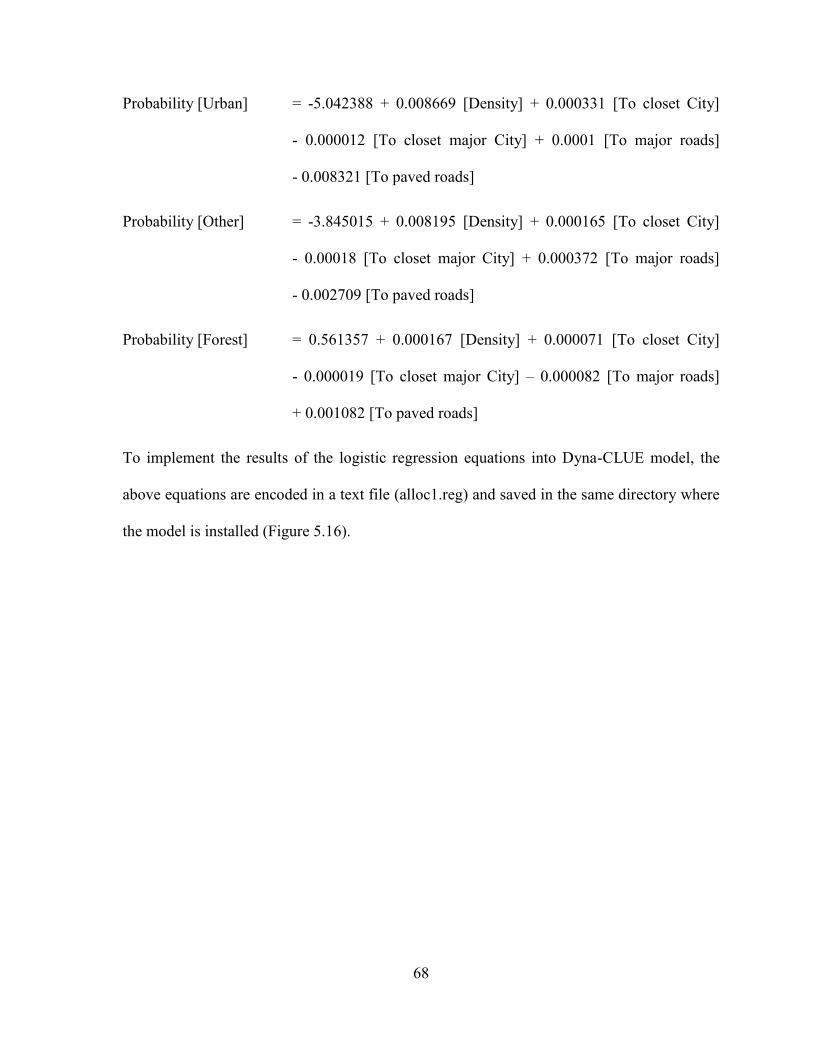
68

Probability [Urban] = -5.042388 + 0.008669 [Density] + 0.000331 [To closet City]

- 0.000012 [To closet major City] + 0.0001 [To major roads]

- 0.008321 [To paved roads]

Probability [Other] = -3.845015 + 0.008195 [Density] + 0.000165 [To closet City]

- 0.00018 [To closet major City] + 0.000372 [To major roads]

- 0.002709 [To paved roads]

Probability [Forest] = 0.561357 + 0.000167 [Density] + 0.000071 [To closet City]

- 0.000019 [To closet major City] – 0.000082 [To major roads]

+ 0.001082 [To paved roads]

To implement the results of the logistic regression equations into Dyna-CLUE model, the

above equations are encoded in a text file (alloc1.reg) and saved in the same directory where

the model is installed (Figure 5.16).

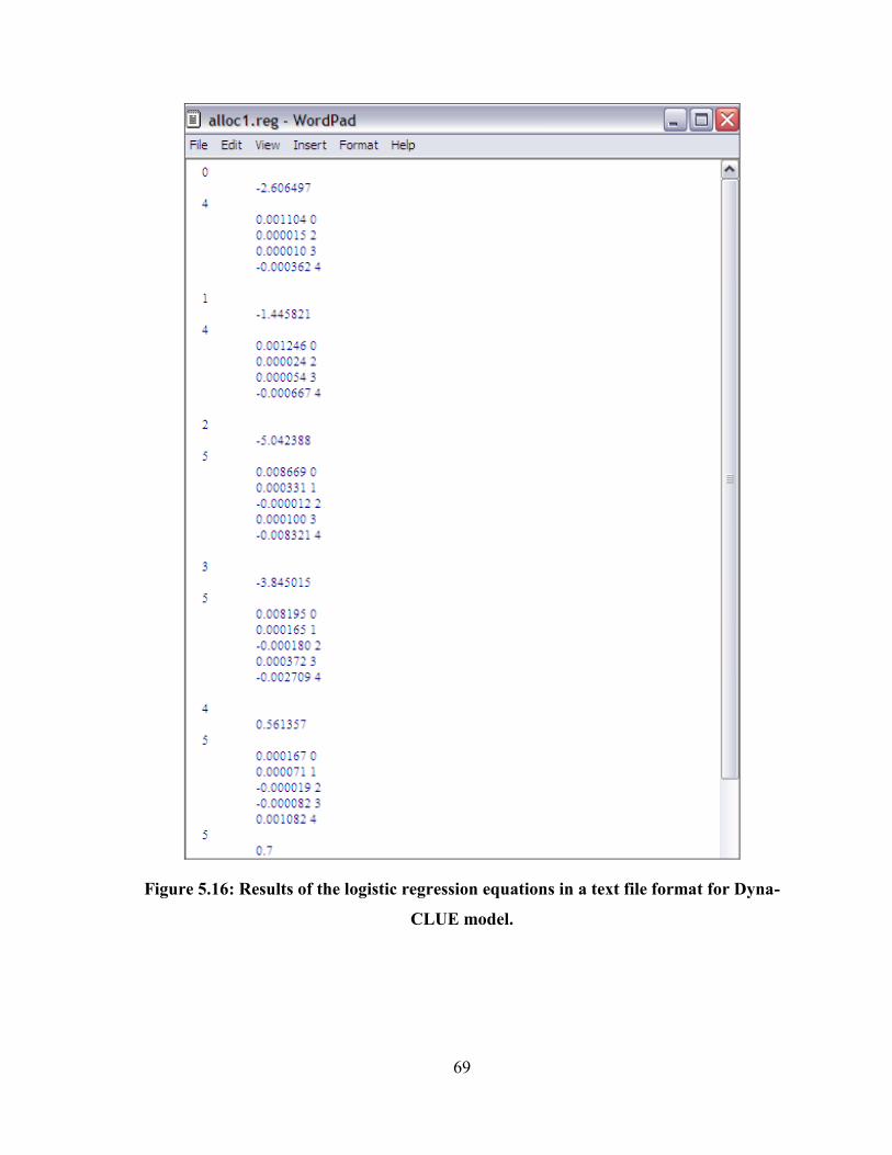
69

Figure 5.16: Results of the logistic regression equations in a text file format for Dyna-

CLUE model.

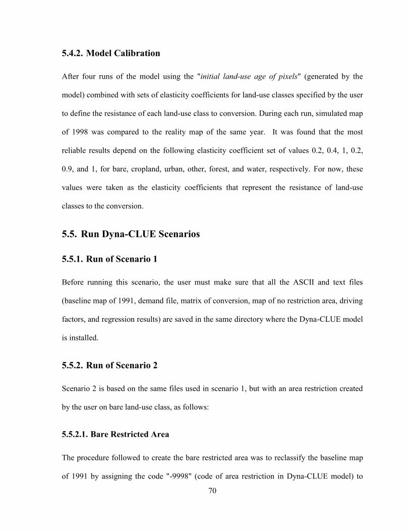
70

5.4.2. Model Calibration

After four runs of the model using the "initial land-use age of pixels" (generated by the

model) combined with sets of elasticity coefficients for land-use classes specified by the user

to define the resistance of each land-use class to conversion. During each run, simulated map

of 1998 was compared to the reality map of the same year. It was found that the most

reliable results depend on the following elasticity coefficient set of values 0.2, 0.4, 1, 0.2,

0.9, and 1, for bare, cropland, urban, other, forest, and water, respectively. For now, these

values were taken as the elasticity coefficients that represent the resistance of land-use

classes to the conversion.

5.5. Run Dyna-CLUE Scenarios

5.5.1. Run of Scenario 1

Before running this scenario, the user must make sure that all the ASCII and text files

(baseline map of 1991, demand file, matrix of conversion, map of no restriction area, driving

factors, and regression results) are saved in the same directory where the Dyna-CLUE model

is installed.


Scenario 2 is based on the same files used in scenario 1, but with an area restriction created

by the user on bare land-use class, as follows:

5.5.2.1. Bare Restricted Area

The procedure followed to create the bare restricted area was to reclassify the baseline map

of 1991 by assigning the code "-9998" (code of area restriction in Dyna-CLUE model) to

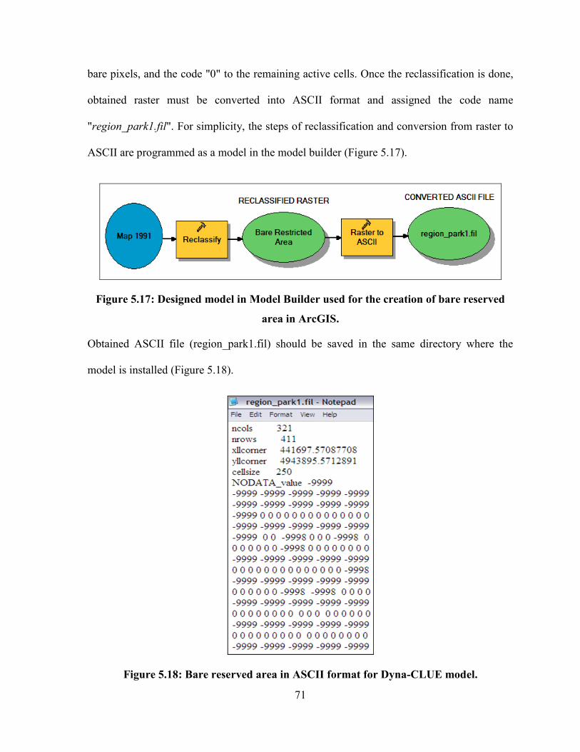
71

bare pixels, and the code "0" to the remaining active cells. Once the reclassification is done,

obtained raster must be converted into ASCII format and assigned the code name

"region_park1.fil". For simplicity, the steps of reclassification and conversion from raster to

ASCII are programmed as a model in the model builder (Figure 5.17).

Figure 5.17: Designed model in Model Builder used for the creation of bare reserved

area in ArcGIS.

Obtained ASCII file (region_park1.fil) should be saved in the same directory where the

model is installed (Figure 5.18).

Figure 5.18: Bare reserved area in ASCII format for Dyna-CLUE model.

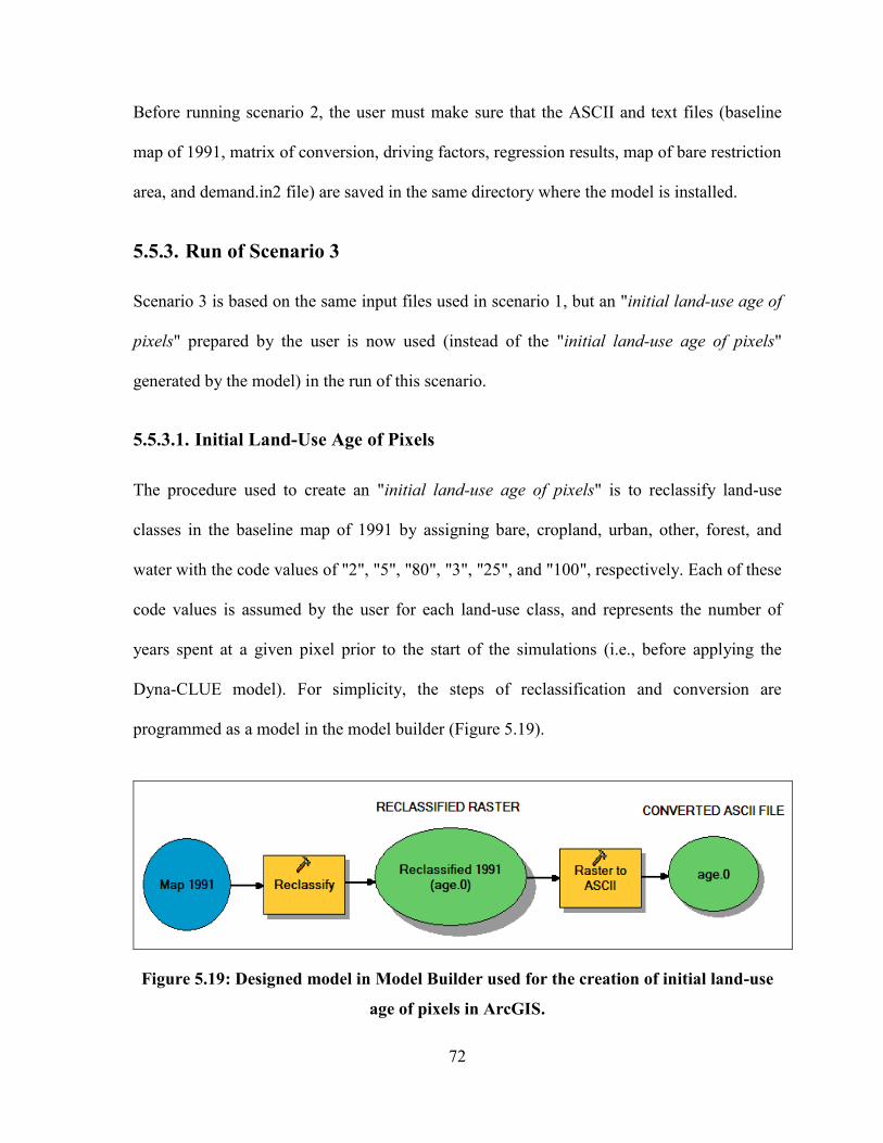
72

Before running scenario 2, the user must make sure that the ASCII and text files (baseline

map of 1991, matrix of conversion, driving factors, regression results, map of bare restriction

area, and demand.in2 file) are saved in the same directory where the model is installed.


Scenario 3 is based on the same input files used in scenario 1, but an "initial land-use age of

pixels" prepared by the user is now used (instead of the "initial land-use age of pixels"

generated by the model) in the run of this scenario.

5.5.3.1. Initial Land-Use Age of Pixels

The procedure used to create an "initial land-use age of pixels" is to reclassify land-use

classes in the baseline map of 1991 by assigning bare, cropland, urban, other, forest, and

water with the code values of "2", "5", "80", "3", "25", and "100", respectively. Each of these

code values is assumed by the user for each land-use class, and represents the number of

years spent at a given pixel prior to the start of the simulations (i.e., before applying the

Dyna-CLUE model). For simplicity, the steps of reclassification and conversion are

programmed as a model in the model builder (Figure 5.19).

Figure 5.19: Designed model in Model Builder used for the creation of initial land-use

age of pixels in ArcGIS.

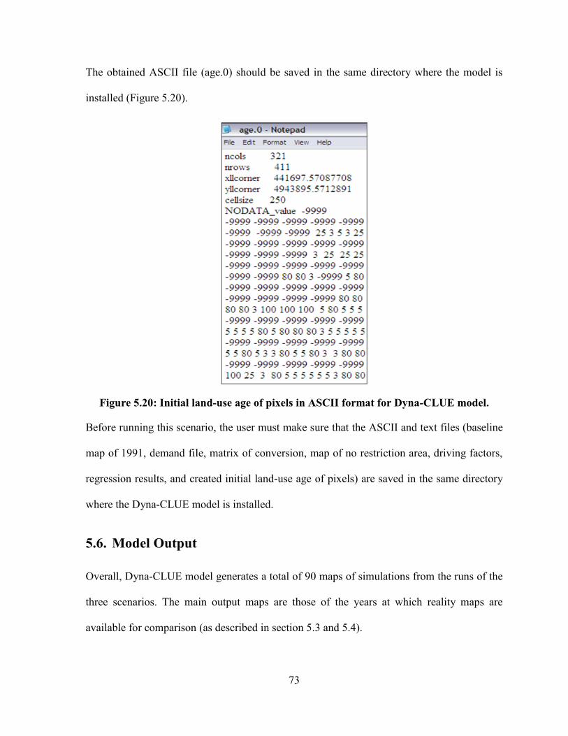
73

The obtained ASCII file (age.0) should be saved in the same directory where the model is

installed (Figure 5.20).

Figure 5.20: Initial land-use age of pixels in ASCII format for Dyna-CLUE model.

Before running this scenario, the user must make sure that the ASCII and text files (baseline

map of 1991, demand file, matrix of conversion, map of no restriction area, driving factors,

regression results, and created initial land-use age of pixels) are saved in the same directory

where the Dyna-CLUE model is installed.

5.6. Model Output

Overall, Dyna-CLUE model generates a total of 90 maps of simulations from the runs of the

three scenarios. The main output maps are those of the years at which reality maps are

available for comparison (as described in section 5.3 and 5.4).

74

5.6.1. Simulated Maps from Scenarios 1 and 3

Taking into consideration the existence of reality maps for the year 1998 (the 7th

year of

simulations) and 2005 (the 14th

year of simulations), only simulated maps of those years (i.e.,

1998 and 2005) are selected to undertake the error matrix tests as shown below in sections

5.7.1.1 and 5.7.1.3.

5.6.2. Simulated Maps from Scenario 2

Only maps of year 2005 (the 14th

year of simulations) and 2020 (last year of simulations) are

selected to undertake the error matrix tests with the baseline map of 1991 (section 5.7.1.2).

5.7. Model Validation

Dyna-CLUE generates maps in ASCII format (without projection) with numbering codes for

land-use classes which start from class "zero". In order to compare between simulated and

reality maps, selected maps must be converted from ASCII to raster, then the projection

parameters of obtained rasters must be adjusted to fit the geographical location of the SN

watershed (e.g., NAD_1983, UTM_Zone 18 N, and D_North_American_1983). After that,

the land-use classes in projected rasters are reclassified with code numbers starting from a

value of "1".

5.7.1. Statistical Validation

5.7.1.1. Validation of Results Generated from Scenario 1

The geo-processing procedures (i.e., the ASCII/raster conversion, raster projection,

reclassification, and computation of the cross-tabulation area between simulated and reality

maps of 1998 and 2005) were programmed as a model in model builder (Figure 5.21). Next,

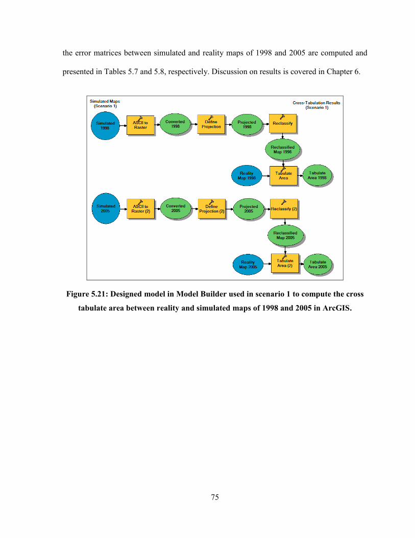
75

the error matrices between simulated and reality maps of 1998 and 2005 are computed and

presented in Tables 5.7 and 5.8, respectively. Discussion on results is covered in Chapter 6.

Figure 5.21: Designed model in Model Builder used in scenario 1 to compute the cross

tabulate area between reality and simulated maps of 1998 and 2005 in ArcGIS.

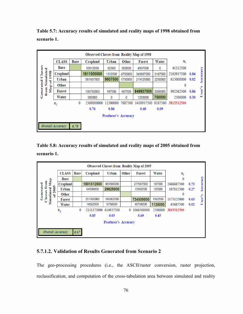
76

Table 5.7: Accuracy results of simulated and reality maps of 1998 obtained from

scenario 1.


scenario 1.




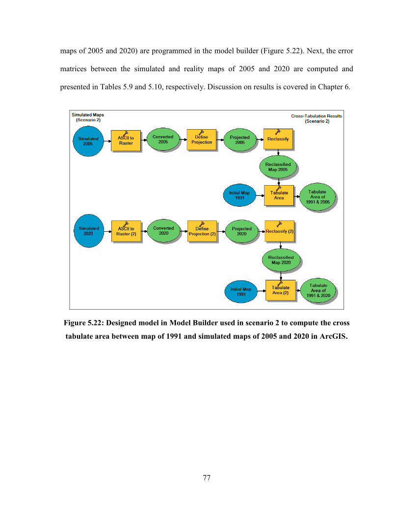
77

maps of 2005 and 2020) are programmed in the model builder (Figure 5.22). Next, the error

matrices between the simulated and reality maps of 2005 and 2020 are computed and

presented in Tables 5.9 and 5.10, respectively. Discussion on results is covered in Chapter 6.


tabulate area between map of 1991 and simulated maps of 2005 and 2020 in ArcGIS.

78

Table 5.9: Accuracy results of map of 1991 and simulated map of 2005 obtained from

scenario 2.

Table 5.10: Accuracy results of map of 1991 and simulated map of 2020 obtained from

scenario 2.




maps of 1998 and 2005) are programmed in the model builder (Figure 5.23).

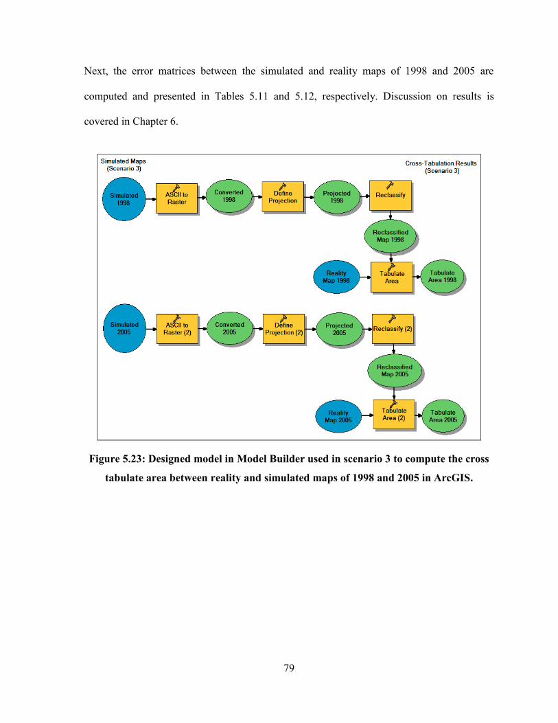
79

Next, the error matrices between the simulated and reality maps of 1998 and 2005 are

computed and presented in Tables 5.11 and 5.12, respectively. Discussion on results is

covered in Chapter 6.


tabulate area between reality and simulated maps of 1998 and 2005 in ArcGIS.

80


scenario 3.


scenario 3.

81

CHAPTER 6

DISCUSSION AND CONCLUSIONS

6.1. Outline

This chapter focuses on the performance of the Dyna-CLUE model in simulating land-use

changes of the South Nation watershed. In order to test the hypotheses proposed in scenarios

1 and 3, the simulated maps of 1998 and 2005, generated from both scenarios, were used to

conduct the error matrices with the reality maps of the same years. To test the hypothesis

proposed in scenario 2, the simulated maps of 2005 and 2020 were used to conduct the error

matrices with the baseline map of 1991. At the end, a visual comparison between the three

scenarios is conducted for the last simulated maps (maps of year 2020) so as to identify the

best scenario(s) in predicting realistic simulations for the SN watershed.

6.2. Results from Scenario 1

6.2.1. Error Matrix of 1998

Table 5.7 shows the results of the error matrix computed between the reality and simulated

maps of 1998. The overall accuracy computed was 70%, which means that the model was

able to agreeably predict the simulated map of year 1998 (Figure 6.1). Table 5.7 shows that

the cell values on the diagonal (of bare and other land-use classes) had pixel count of empty

cells (no matching between reality and simulated maps of 1998). This means that, in some

year before 1998, both land-use classes had been completely converted. This could have

occurred due to two reasons:

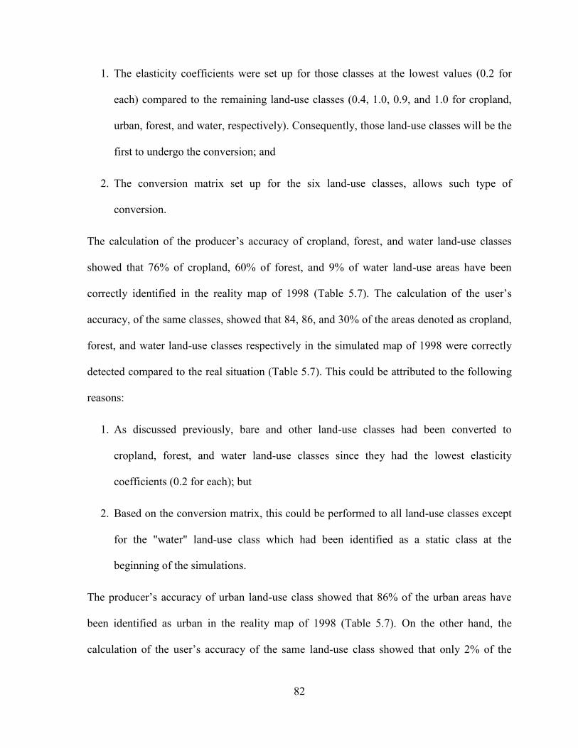
82

1. The elasticity coefficients were set up for those classes at the lowest values (0.2 for

each) compared to the remaining land-use classes (0.4, 1.0, 0.9, and 1.0 for cropland,

urban, forest, and water, respectively). Consequently, those land-use classes will be the

first to undergo the conversion; and

2. The conversion matrix set up for the six land-use classes, allows such type of

conversion.

The calculation of the producer’s accuracy of cropland, forest, and water land-use classes

showed that 76% of cropland, 60% of forest, and 9% of water land-use areas have been

correctly identified in the reality map of 1998 (Table 5.7). The calculation of the user’s

accuracy, of the same classes, showed that 84, 86, and 30% of the areas denoted as cropland,

forest, and water land-use classes respectively in the simulated map of 1998 were correctly

detected compared to the real situation (Table 5.7). This could be attributed to the following

reasons:

1. As discussed previously, bare and other land-use classes had been converted to

cropland, forest, and water land-use classes since they had the lowest elasticity

coefficients (0.2 for each); but

2. Based on the conversion matrix, this could be performed to all land-use classes except

for the "water" land-use class which had been identified as a static class at the

beginning of the simulations.

The producer’s accuracy of urban land-use class showed that 86% of the urban areas have

been identified as urban in the reality map of 1998 (Table 5.7). On the other hand, the

calculation of the user’s accuracy of the same land-use class showed that only 2% of the

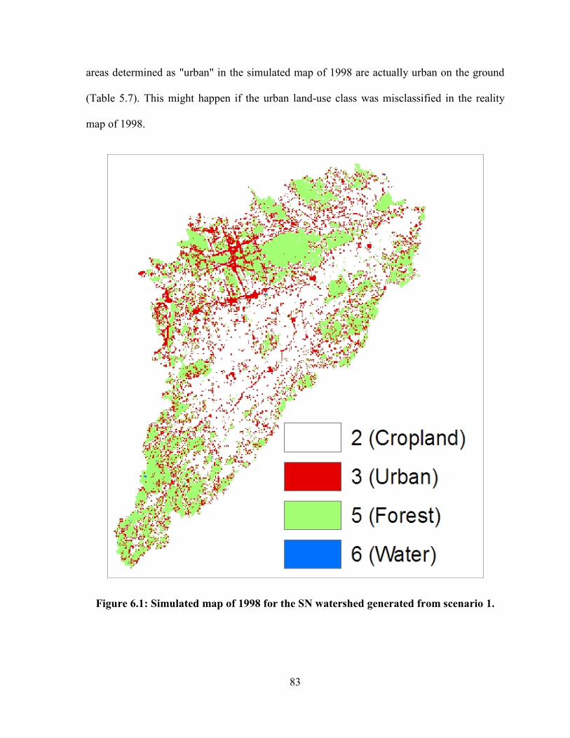
83

areas determined as "urban" in the simulated map of 1998 are actually urban on the ground

(Table 5.7). This might happen if the urban land-use class was misclassified in the reality

map of 1998.

Figure 6.1: Simulated map of 1998 for the SN watershed generated from scenario 1.

84

6.2.2. Error Matrix of 2005

Table 5.8 shows the results of the error matrix computed between the reality and simulated

maps of 2005. The overall accuracy of the model was 67%, which means that simulated map

of 2005 (Figure 6.2) was fairly close to the reality map of the same year.

The producer’s accuracy computed for the model predictions of cropland, forest, and water

land-use classes have shown that 85% of cropland, 69% of forest, and 45% of water land-use

areas have been correctly identified in the reality map of 2005 (Table 5.8). While, the

calculation of the user’s accuracy for the same classes showed that only 73% , 63%, and 2%

of the areas identified as cropland, forest, and water land-use classes in the simulated map of

2005, were actually cropland, forest, and water land-use classes, respectively, on the ground

(Table 5.8). This could be explained by the reason that cropland, forest, and water classes

might have been misclassified in the reality map of 2005.

The calculation of the producer’s accuracy of urban land-use class showed that only 5% of

the urban areas have been identified as "urban" in the reality map of 2005 (Table 5.8). While,

the calculation of the user’s accuracy, of the same land-use class, showed that 27% of the

areas determined as "urban" in the simulated map of 2005, are actually urban on the ground

(Table 5.8). Since this scenario was run with an initial land-use age of pixels generated by

the model (randomly selected by model), it can be concluded that:

1. The randomized initial land-use age of pixels has played the main role of

synchronizing the rate of conversion among land-use classes;

85

2. Among the remaining land-use classes (cropland, forest, and water), the elasticity

coefficient of cropland was set up at the lowest value (0.4). Therefore, it will be the

first land-use class to undergo the conversion; and

3. The matrix of conversion set up for the six land-use classes allows such type of

conversion.

Figure 6.2: Simulated map of 2005 for the SN watershed generated from scenario 1.

86

6.2.3. Summary from Scenario 1

The results from both error matrices of 1998 and 2005 proved that the Dyna-CLUE model

was able to simulate maps fairly close to reality. It should be noted that the accuracy of

prediction could have been increased with the precision in the reclassification occurred to

original land-use classes of the reality maps of 1998 and 2005. Results are in agreement with

studies conducted by: Verburg and Overmars (2007); Trisurat et al., (2010); Luo et al.,

(2010); and Zhu et al., (2010) which reported that the model was capable of generating

simulated maps quite similar to reality.

The model was found very sensitive to changes in the elasticity coefficients set up for land-

use classes, which conform to the findings of Soepboer (2001); Batisani and Yarnal (2009);

and Luo et al., (2010). The randomized initial land-use age of pixels played a significant role

in synchronizing the rate of conversion among land-use classes, as well as, its direct effect on

calibrating the model’s iteration process. In addition, the combination between the statistical

results of the error matrices and the performance of the model allowed the user to detect

possible misclassification among land-use classes in the reality maps of 1998 and 2005. In

conclusion, the hypotheses proposed for the run of scenario 1 was proved true.


6.3.1. Error Matrices of 2005 and 2020

In the error matrices presented in Tables 5.9 and 5.10, the producer’s and user’s accuracies

for the predictions of bare land-use were equal to 100%, which indicates that bare land-use

type have not undergone any conversions and was stable during the whole simulation period.

In addition, validation by visual observation between the baseline map of 1991 and the

87

simulated maps of 2005 and 2020 confirmed that bare areas remained intact during the

simulation period (Figure 6.3).

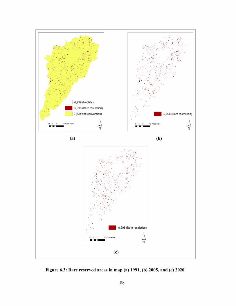
88

(a) (b)

(c)

Figure 6.3: Bare reserved areas in map (a) 1991, (b) 2005, and (c) 2020.

89

6.3.2. Summary from Scenario 2

The results of statistical and visual validation conducted between the baseline map of 1991

and the simulated maps of 2005 and 2020 proved that the Dyna-CLUE model was able to

respond to any planned policies (such as that proposed in scenario 2). Results are in

agreement with the findings of Soepboer (2001); Verburg and Overmars (2007); Luo et al.,

(2010); and Zhu et al., (2010) who reported that the Dyna-CLUE model is generally capable

of respond and protect policy-making of any reserved areas. In conclusion, the hypotheses

proposed for the run of scenario 2 was verified.


6.4.1. Error Matrices of 1998 and 2005

Tables 5.11 and 5.12 shows the same results of the error matrices as observed in tables 5.7

and 5.8 computed between the reality and simulated maps of 1998 and 2005, respectively.

Such results proved that the initial land-use age of pixels created by the user and

implemented in the run of scenario 3 was found not to play a role in synchronizing and

prioritizing the sequences of conversions among land-use classes as was expected.

6.5. Comparison between Scenarios

This comparison covers only the results generated from scenarios 1 and 2, since scenario 3

was found identical to scenario 1.

Scenario 2 was conducted as a test to assess the ability of the Dyna-CLUE model to respond

to a proposed policy. Therefore, the following conclusions can be drawn:

1. The Dyna-CLUE model was able to fairly simulate/predict reality maps (scenario 1).

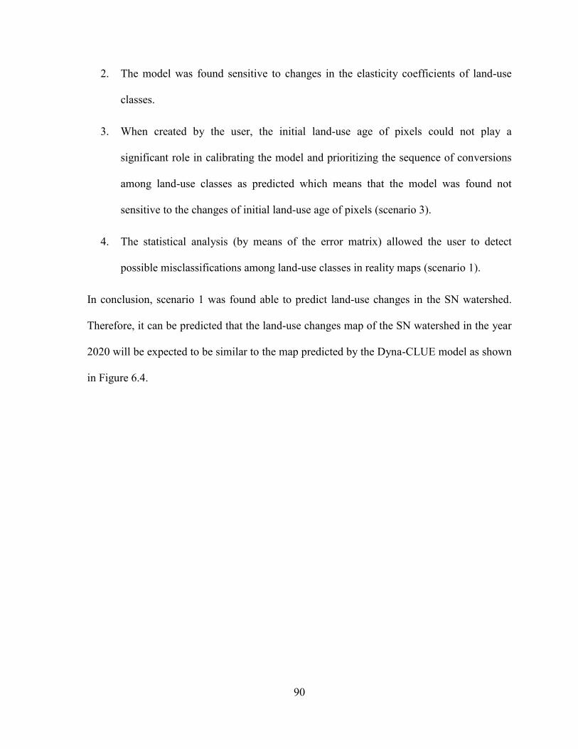
90

2. The model was found sensitive to changes in the elasticity coefficients of land-use

classes.

3. When created by the user, the initial land-use age of pixels could not play a

significant role in calibrating the model and prioritizing the sequence of conversions

among land-use classes as predicted which means that the model was found not

sensitive to the changes of initial land-use age of pixels (scenario 3).

4. The statistical analysis (by means of the error matrix) allowed the user to detect

possible misclassifications among land-use classes in reality maps (scenario 1).

In conclusion, scenario 1 was found able to predict land-use changes in the SN watershed.

Therefore, it can be predicted that the land-use changes map of the SN watershed in the year

2020 will be expected to be similar to the map predicted by the Dyna-CLUE model as shown

in Figure 6.4.

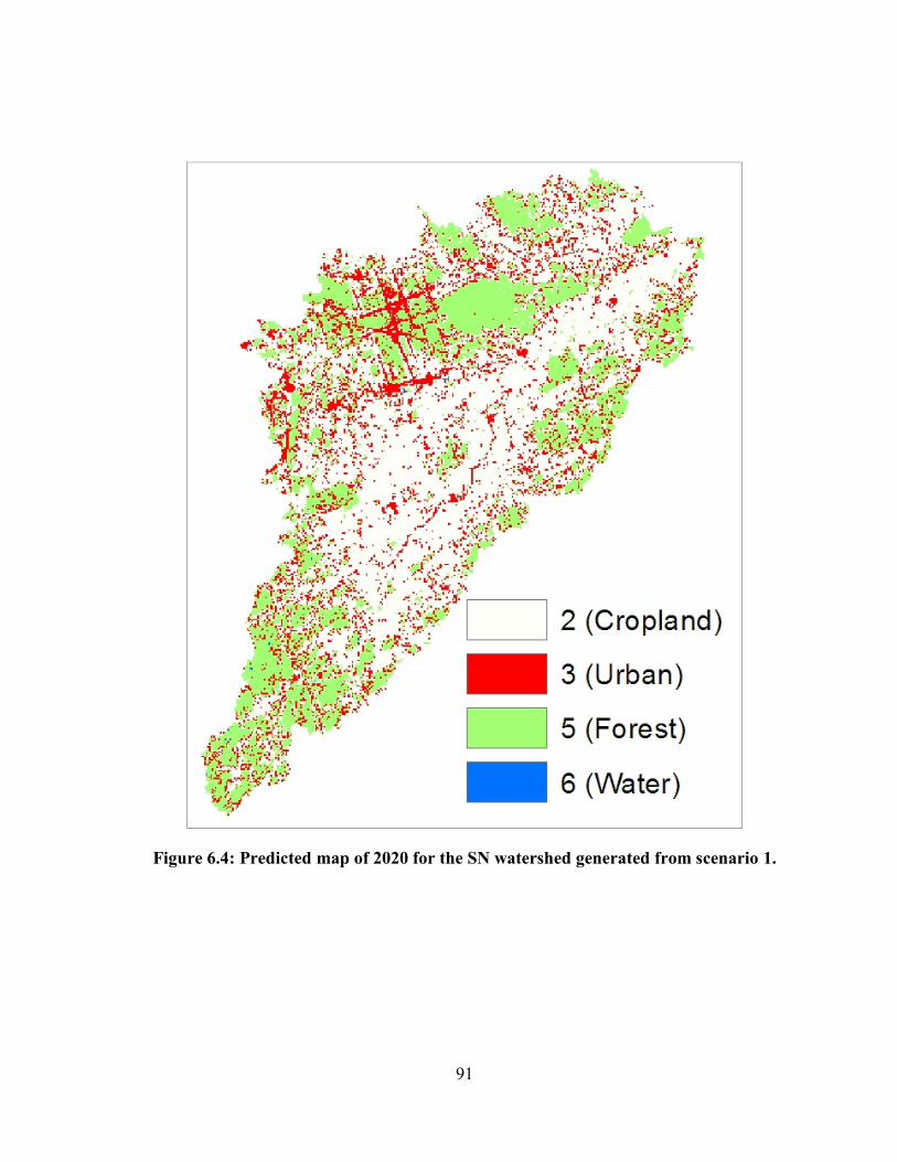
91

Figure 6.4: Predicted map of 2020 for the SN watershed generated from scenario 1.

92

6.6. Conclusions

The Dyna-CLUE model was applied to the South Nation watershed with three different runs

of scenarios in order to have a better understanding of the development of the region. Based

on the simulations performed in the present study, it should be noted that the application of

the Dyna-CLUE model is not straightforward since data preparation and conversions require

significant time (months). In addition, basic knowledge and expertises in statistical software

(SPSS or other) and ArcGIS are required to run statistical analyses and geo-processing

procedures.

The interpretation of the results of this study proved that, the Dyna-CLUE model was able

to: (1) simulate land-use maps quite close to reality, and (2) respond to proposed policies

such as certain area restrictions. It was found that the model was not sensitive to the

implementation of an initial land-use age of pixels either randomized by the model or created

by the user. It was also found that the model is very sensitive to changes in the elasticity

coefficients set up for various land-use classes. However, further studies and applications

may contribute to better predict future land-use changes of the region.

6.7. Thesis Contribution

This work is the first application of the Dyna-CLUE model in Eastern Ontario. The research

work in the present study has added the following contributions:

1. Proving that the Dyna-CLUE model was not been affected by implementing an initial

land-use age of pixels created by the user. Results observed were the same compared

to those obtained from a run with a randomized initial land-use age of pixels

generated by the model.

93

2. Enhancing the common statistical validation procedures of the model by calculating

the error matrix (map pair analysis) between simulated and reality maps at a given

year.

6.8. Future Work and Recommendations

Based on the observations and findings of this study, the following recommendations are

proposed for future work intended to apply the Dyna-CLUE modeling software:

1. The conservation authority of the South Nation watershed should develop and

enforce sustainable policies, such as: specify park zones with forestry regions,

agricultural zoning and recreational/tourism zoning, so as to better control the

urbanization growth in the watershed.

2. For future studies of the South Nation watershed, the modeller must consider

implementing some socio-economic drivers (e.g., income and gross domestic

product) as well as bio-physical drivers (such as soil erosion susceptibility).

3. In the calculation of the land-use demands, the modeller must rely on socio-economic

trends to project future allocated areas since those trends are more realistic in figuring

out the situation rather than historical trends.

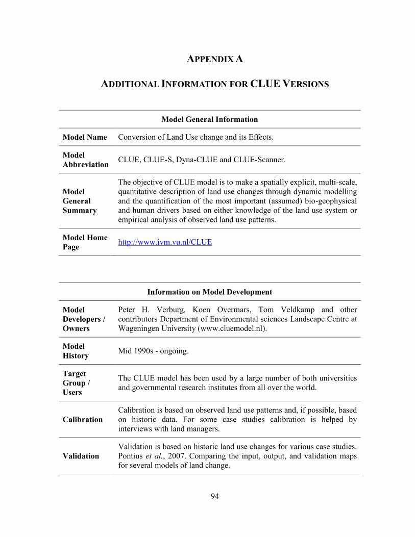
94

APPENDIX A

ADDITIONAL INFORMATION FOR CLUE VERSIONS

Model General Information

Model Name Conversion of Land Use change and its Effects.

Model

Abbreviation CLUE, CLUE-S, Dyna-CLUE and CLUE-Scanner.

Model

General

Summary

The objective of CLUE model is to make a spatially explicit, multi-scale,

quantitative description of land use changes through dynamic modelling

and the quantification of the most important (assumed) bio-geophysical

and human drivers based on either knowledge of the land use system or

empirical analysis of observed land use patterns.

Model Home

Page http://www.ivm.vu.nl/CLUE

Information on Model Development

Model

Developers /

Owners

Peter H. Verburg, Koen Overmars, Tom Veldkamp and other

contributors Department of Environmental sciences Landscape Centre at

Wageningen University (www.cluemodel.nl).

Model

History Mid 1990s - ongoing.

Target

Group /

Users

The CLUE model has been used by a large number of both universities

and governmental research institutes from all over the world.

Calibration

Calibration is based on observed land use patterns and, if possible, based

on historic data. For some case studies calibration is helped by

interviews with land managers.

Validation

Validation is based on historic land use changes for various case studies.

Pontius et al., 2007. Comparing the input, output, and validation maps

for several models of land change.

http://www.ivm.vu.nl/CLUE

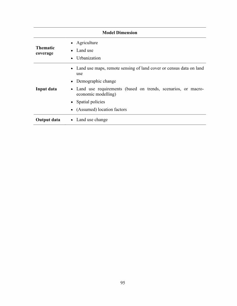
95

Model Dimension

Thematic

coverage

Agriculture

Land use

Urbanization

Input data

Land use maps, remote sensing of land cover or census data on land

use

Demographic change

Land use requirements (based on trends, scenarios, or macro-

economic modelling)

Spatial policies

(Assumed) location factors

Output data Land use change

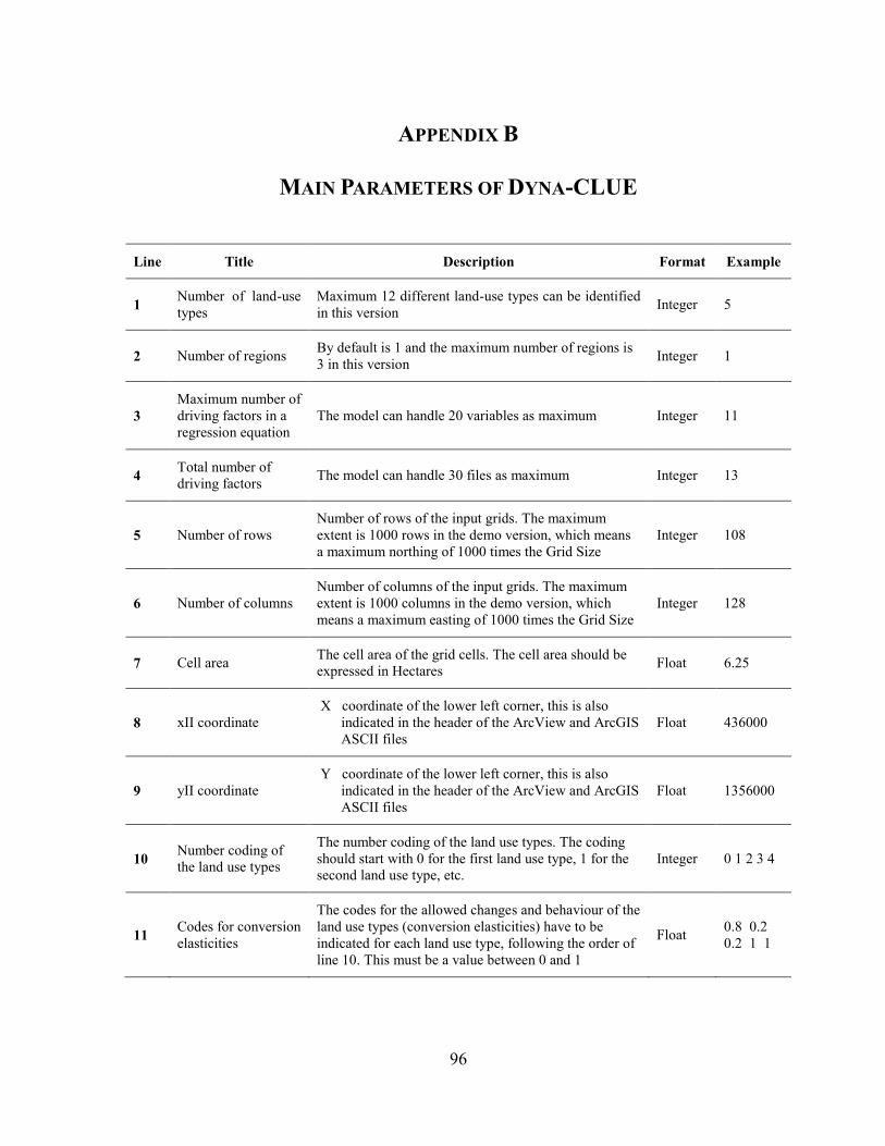
96

APPENDIX B

MAIN PARAMETERS OF DYNA-CLUE

Line Title Description Format Example

1 Number of land-use

types

Maximum 12 different land-use types can be identified

in this version Integer 5

2 Number of regions By default is 1 and the maximum number of regions is

3 in this version Integer 1

3

Maximum number of

driving factors in a

regression equation

The model can handle 20 variables as maximum Integer 11

4 Total number of

driving factors The model can handle 30 files as maximum Integer 13

5 Number of rows

Number of rows of the input grids. The maximum

extent is 1000 rows in the demo version, which means

a maximum northing of 1000 times the Grid Size

Integer 108

6 Number of columns

Number of columns of the input grids. The maximum

extent is 1000 columns in the demo version, which

means a maximum easting of 1000 times the Grid Size

Integer 128

7 Cell area The cell area of the grid cells. The cell area should be

expressed in Hectares Float 6.25

8 xII coordinate

X coordinate of the lower left corner, this is also

indicated in the header of the ArcView and ArcGIS

ASCII files

Float 436000

9 yII coordinate

Y coordinate of the lower left corner, this is also

indicated in the header of the ArcView and ArcGIS

ASCII files

Float 1356000

10 Number coding of

the land use types

The number coding of the land use types. The coding

should start with 0 for the first land use type, 1 for the

second land use type, etc.

Integer 0 1 2 3 4

11 Codes for conversion

elasticities

The codes for the allowed changes and behaviour of the

land use types (conversion elasticities) have to be

indicated for each land use type, following the order of

line 10. This must be a value between 0 and 1

Float 0.8 0.2

0.2 1 1

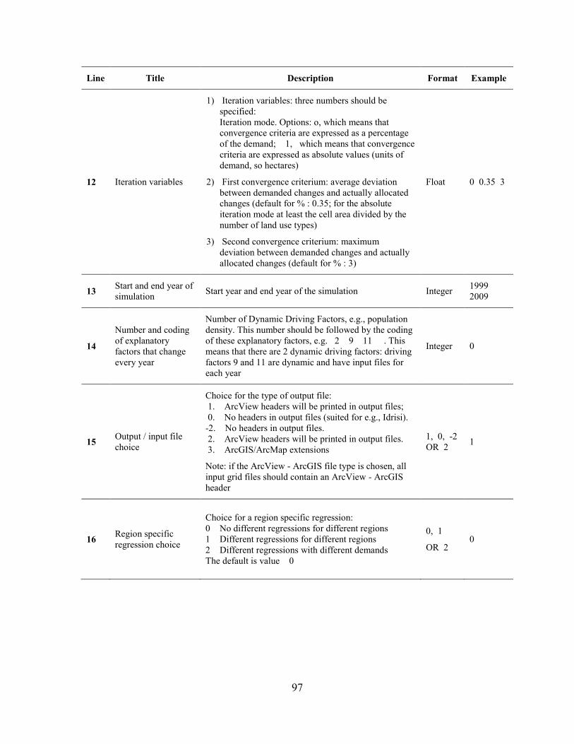
97


12 Iteration variables

1) Iteration variables: three numbers should be

specified:

Iteration mode. Options: o, which means that

convergence criteria are expressed as a percentage

of the demand; 1, which means that convergence

criteria are expressed as absolute values (units of

demand, so hectares)

2) First convergence criterium: average deviation

between demanded changes and actually allocated

changes (default for % : 0.35; for the absolute

iteration mode at least the cell area divided by the

number of land use types)

3) Second convergence criterium: maximum

deviation between demanded changes and actually

allocated changes (default for % : 3)

Float 0 0.35 3

13 Start and end year of

simulation Start year and end year of the simulation Integer

1999

2009

14

Number and coding

of explanatory

factors that change

every year

Number of Dynamic Driving Factors, e.g., population

density. This number should be followed by the coding

of these explanatory factors, e.g. 2 9 11 . This

means that there are 2 dynamic driving factors: driving

factors 9 and 11 are dynamic and have input files for

each year

Integer 0

15 Output / input file

choice

Choice for the type of output file:

1. ArcView headers will be printed in output files;

0. No headers in output files (suited for e.g., Idrisi).

-2. No headers in output files.

2. ArcView headers will be printed in output files.

3. ArcGIS/ArcMap extensions

Note: if the ArcView - ArcGIS file type is chosen, all

input grid files should contain an ArcView - ArcGIS

header

1, 0, -2

OR 2 1

16 Region specific

regression choice

Choice for a region specific regression:

0 No different regressions for different regions

1 Different regressions for different regions

2 Different regressions with different demands

The default is value 0

0, 1

OR 2 0

98


17 Initialization of land

use history

0 the initial land use history will be read from file

age.0, which should contain a grid with, for every

pixel, the number of years that the pixel is used for the

current land use type

1 a random number will be assigned to all pixels to

represent the number of years that the current land use

is already found at that location according to the

standard seed for the random number generator. with

this option two runs will result in the same random

number, which is useful for comparison

2 a random number will be assigned to all pixels to

represent the number of years that the current land use

is already found at the location with a different random

number generator.

For option 1 or 2 an additional number should be added

that indicates the maximum number of years that can

be generated by the randomizer (5 in the example

below)

0, 1

OR 2 1 5

18 Neighbourhood

calculation choice

Choice for using the neighborhood function:

0 Neighbourhood function is not used

1 Neighbourhood function is used in simulation

2 Only the influences are calculated

0, 1

OR 2 2

19 Location specific

preference addition

Variables for location specific preference addition. The

first number is a switch: activate the function (1) or not

(0). If the switch is set to 1 , it should be followed by,

for each land use type, the fraction of the preference

addition that is added to the probability as calculated in

the regression

Integer 0

20 Optimal iteration

parameter

Iteration parameter. If no value is supplied 0.05 is

assumed which works well with most applications. The

value of this parameter should be between 0.001 and

0.1. With a somewhat higher value (e.g. 0.06) the

iteration is more stabile and more likely to find a

solution. A lower value (e.g. 0.01) will give a faster

convergence although instability is more likely

Float 0

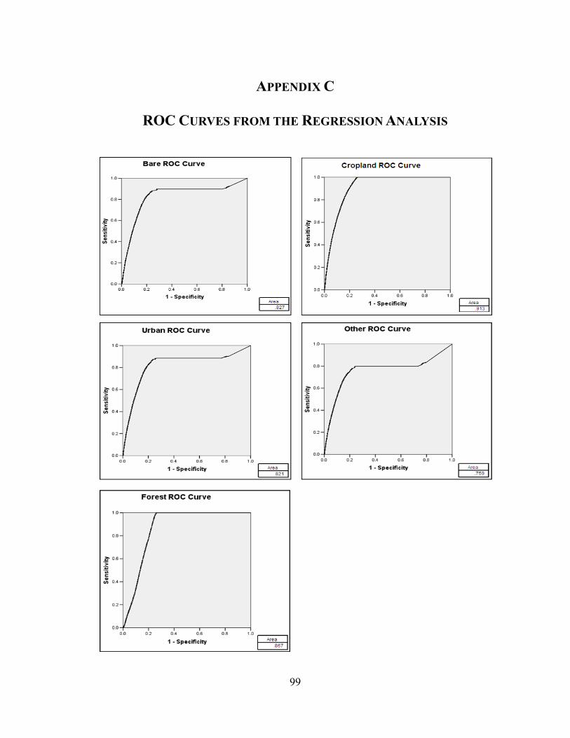
99

APPENDIX C

ROC CURVES FROM THE REGRESSION ANALYSIS

100

REFERENCES

Batisani, N, Yarnal, B. (2009) Urban expansion in Centre County, Pennsylvania: spatial

dynamics and landscape transformations. Applied Geography 29, 235-249.

Benders, R.M.J. (1996) Interactive Simulation of Electricity Demand and Production. PhD

Thesis, Groningen University, Groningen, The Netherlands.

Bingner, R., Theurer, F., Yuan, Y. (2007) AnnAGNPS Technical Processes. Available at:

ftp://199.133.90.201/pub/outgoing/AGNPS/AGNPS_Web_Files/pdf_files/AnnAGNPS_

Technical_Documentation.pdf (June 2009).

Bonham-Carter, G.F. (1994) Geographic Information Systems for Geoscientists: Modeling

with GIS, Pergamon, Oxford, United Kingdom.

Briassoulis, H. (2000) Analysis of Land-use Change: Theoretical and Modeling Approaches.

The web book of regional science. West Virginia University, Regional Research

Institute, Morgantown, VA. Available at:

http://www.rri.wvu.edu/WebBook/Briassoulis/contents.htm. (January 2005).

Brown, D.G., Walker, R., Manson, S., Seto, K. (2004) Modeling land use and land cover

change. In: Gutman, G., Janetos, A.C., Justice, C.O., Moran, E.F., Mustard, J.F.,

Rindfuss, R.R., Skole, D.L., Turner, B.L., Cochrane, M.A. (Eds.) Land Change Science:

Observing, Monitoring and Understanding Trajectories of Change on the Earth’s

Surface. Springer, New York, NY, 395-409.

Carter, H. (1981) The Study of Urban Geography. 3rd edition, Edward Arnold, New York,

NY.

Cheng, J. (2003) Modelling Spatial and Temporal Urban Growth. PhD Thesis, Utrecht

University, Utrecht, The Netherlands.

Congalton, R.G., Green, K. (1999) Assessing the Accuracy of Remotely Sensed Data -

Principles and Practices, 1st Edition, CRC Press, Lewis Publishers, Boca Raton, FL.

Coyne, P. (2001) Reflections of the South Nation Watershed: A Pictorial History of Its

People and Natural Resources. General Store Publishing House, Burnstown, ON.

ftp://199.133.90.201/pub/outgoing/AGNPS/AGNPS_Web_Files/pdf_files/AnnAGNPS_Technical_Documentation.pdf

ftp://199.133.90.201/pub/outgoing/AGNPS/AGNPS_Web_Files/pdf_files/AnnAGNPS_Technical_Documentation.pdf

http://www.rri.wvu.edu/WebBook/Briassoulis/contents.htm

101

Di Gregorio, A. (2005) Land Cover Classification System (LCCS), version 2: Classification

Concepts and User Manual. FAO Environment and Natural Resources Service Series,

No. 8, Rome, Italy.

Diogo, B., Azzah, J. (1995) The St. Lawrence Ecosystem: From Iroquois Dam to the

Beauharnois Dam: A Socio-Economic Profile. Institute for Research on Environment

and Economy, University of Ottawa, Ottawa, ON.

Dodd, L.E., Pepe, M.S. (2003) Semiparametric regression for the area under the receiver

operating characteristic curve. Journal of the American Statistical Association, 98, 409-

417.

Engelsman, W. (2002) Simulating land-use change in an urbanising area Malaysia. Thesis

Report, Wageningen University, Wageningen, The Netherlands.

Garson, G.D. (2005) Statnotes: Topics in Multivariate Analysis. Available on:

http://www2.chass.ncsu.edu/garson/pa765/statnote.htm.

Jinyan, Z., Xiangzheng, D., Qun’ou, J., Nana, S. (2007) The application of system dynamics

and CLUE-S model in land use change dynamic simulation: a case study in Taips

County, Inner Mongolia of China. Proceedings of the Conference on System Science,

Management Science & System Dynamics, 2781-2790.

Kaimowitz, D., Angelsen, A. (1998) Economic Models of Tropical Deforestation: A Review.

Center for International Forestry research, Borgor, Indonesia.

Lambin, E.F. (2004) Modelling Land-Use Change. In: John, W., Mulligan, M. (Eds.)

Environmental Modelling: Finding Simplicity in Complexity. John Wiley & Sons, Inc.,

West Sussex, London.

Lambin, E.F., Geist, H.J. (2002) Proximate causes and underlying driving forces of tropical

deforestation. BioScience, 52(2), 143-150.

Lambin, E.F., Rounsevell, M.D.A., Geist, H.J. (2000) Are agricultural land-use models able

to predict changes in land-use intensity?. Agriculture, Ecosystems and Environment, 82,

321-331.

http://www2.chass.ncsu.edu/garson/pa765/statnote.htm

102

Luo, G.P., Chen, X., Zhou, K.f., Ye, M.Q. (2003) Temporal and spatial variation and

stability of the oasis in the Sangong River Watershed. Science in China, Series D46 (1),

62-73.

Luo, G., Yin, C., Chen, X., Xu, W., Lu, L. (2010) Combining system dynamic model and

CLUE-S model to improve land use scenario analyses at regional scale: A case study of

Sangong watershed in Xinjiang, China. Ecological Complexity, 7(2), 198-207.

Lusted L.B. (1971) Signal detectability and medical decision-making. Science, 171, 1217-

1219.

Meadows, D.H., Randers, J., Meadows, D.L. (2004) The Limits to Growth: The 30-Year

Update. 3rd

Edition, Chelsea Green, White River Junction, VT.

Mulligan, M., Wainwright, J. (2004) Modelling and Model Building. In: Wainwright, J.,

Mulligan, M. (Eds.). Environmental Modelling: Finding Simplicity in Complexity. John

Wiley & Sons, Inc., West Sussex, London.

Obuchowski, N.A. (2003) Receiver operating characteristic curves and their use in radiology.

Radiology, 229(1), 3-8.

Palang, H., Mander, U., Naveh, Z. (2000) Holistic landscape ecology in action. Landscape

and Urban Planning, 50, 1-6.

Perez-Soba, M., Verburg, P.H., Koomen, E., Hilferink, M., Benito, P., Banse, M., Woltjer,

G., Eichhout, B., Prins, A.-G., Staritsky, I. (2010) Land Use Modelling-Implementation;

Preserving and Enhancing the Environmental Benefits of “Land-Use Services”. Final

report to the European Commission, DG Environment. Alterra Wageningen UR, Geodan

Next, Object Vision, BIOS, LEI and PBL, Wageningen, The Netherlands.

Pontius, R., Boersma, W., Castella, J.C., Clarke, K., de Nijs, T., Dietzel, C., Duan, Z.,

Fotsing, E., Goldstein, N., Kok, K., Koomen, E., Lippitt, C., McConnell, W., Mohd

Sood, A., Pijanowski, B., Pithadia, S., Sweeney, S., Trung, T., Veldkamp, A. and

Verburg, P. (2004) Comparing the input, output, and validation maps for several models

of land change, The Annals of Regional Science, 42(1), 11-37.

103

Pontius, R.G., Schneider, L.C. (2001) Land-cover change model validation by an ROC

method for the Ipswich watershed, Massachusetts, USA. Agriculture Ecosystems &

Environment, 85, 239-248.

Riebsame, W.E., Meyer, W.B., Turner II, B.L. (1994) Modeling land use and cover as part of

global environmental change. Climatic Change, 28, 45-64.

Seidou, O., Lapen, D. (2010) Land Use Changes in the South Nation Watershed, 1966-2050.

AAFC – Agriculture and Agri-food Canada.

SNC (South Nation Conservation) (2006) Clean Water Program Annual Report. Available

on: http://www.nation.on.ca.

Soepboer, W. (2001) The Conversion of Land Use and its Effects at Small regional extent

CLUE-S. An application for the Sibuyan Island, The Philippines. MSc Thesis,

Wageningen University, Wageningen, The Netherlands.

Tian, G.C.C., Jinhong, D., Wei, Y. (1993) The study of the urban fringes in Chinese

megalopolises. Acta Geographical Sinica, 48(4), 317-328.

Torrens, P.M. (2000). How land-use transportation models work. Centre for Advanced

Spatial Analysis. Working Paper Series, 20, 6-75.

Trisurat, Y., Alkemade, R., Verburg, P. (2010) Projecting land-use change and its

consequences for biodiversity in northern Thailand. Environmental Management, 45(3),

626-639.

Turner II, B.L., Skole, D.L., Sanderson, S., Fischer, G., Fresco, L.O., Leemans, R. (1995)

Land-Use and Land-Cover Change - Science/Research Plan. IGBP Report No. 35.

Stockholm, Sweden.

Van den Berg, L.M. (1984) Anticipating Urban Growth in Africa. Occasional Study, Zambia

Geographical Association, Lusaka, Zambia.

Veldkamp, A., Fresco, L.O. (1996) CLUE: a conceptual model to study the conversion of

land use and its effects. Ecological Modeling, 85, 253-270.

Verburg, P.H., Groot, W.T., Veldkamp, A. (2003) Methodology for Multi-Scale Land-Use

Change Modelling: Concepts and Challenges. In: Dolman, A.J, Verhagen, A., Rovers,

104

C.A. (Eds.) Global Environmental Change and Land Use. Kluwer Academic Publishers,

Norwell, MA.

Verburg, P.H., Overmars, K.P. (2007) Dynamic Simulation of Land-Use Change Trajectories

with the CLUE-S Model. In: Koomen, E., Stillwell, J., Bakema, A., Scholten, H.J. (Eds.)

Modelling Land-Use Change: Progress and applications,: Springer, Dordrecht, The

Netherlands.

Verburg, P.H., Overmars, K.P. (2009) Combining top-down and bottom-up dynamics in land

use modeling: exploring the future of abandoned farmlands in Europe with the Dyna-

CLUE model. Landscape Ecology, 24(9), 1167-1181.

Verburg, P.H., Soepboer, W., Limpiada, R., Espaldon, M.V.O., Sharifa, M., Veldkamp, A.

(2002) Land use change modelling at the regional scale: the CLUE-S model.

Environmental Management, 30, 391-405.

Verburg, P.H., Veldkamp, A., de Koning, G.H.J., Kok, K., Bouma, J. (2000) A spatial

explicit allocation procedure for modelling the pattern of land use change based upon

actual land use. Ecological Modelling, 116, 45-61.

Visser, H. (2004) The Map Comparison Kit: methods, software and applications. RIVM

report 550002005/2004, Bilthoven, BA.

Wasserman, L. (2004) All of Statistics: A Concise Course in Statistical Inference. Springer,

New York, NY.

White, R., Engelen, D., Uljee, I. (1997) The use of constrained cellular automata for high

resolution modelling of urban land-use dynamics. Environment and Planning B:

Planning and Design, 24(3), 323-343.

Zhu, Z., Liu, L., Chen, Z., Zhang, J., Verburg, P.H. (2010) Land-use change simulation and

assessment of driving factors in the loess hilly region: a case study as Pengyang County.

Environmental Monitoring and Assessment, 164(1-4), 133-142.

Documents

Modeling Land-Use Changes in the South Nation Watershed ... Khoury_Antoun... · Modeling Land-Use Changes in the South Nation Watershed using Dyna-CLUE by Antoun El Khoury A Thesis