Embed Size (px)
Citation preview
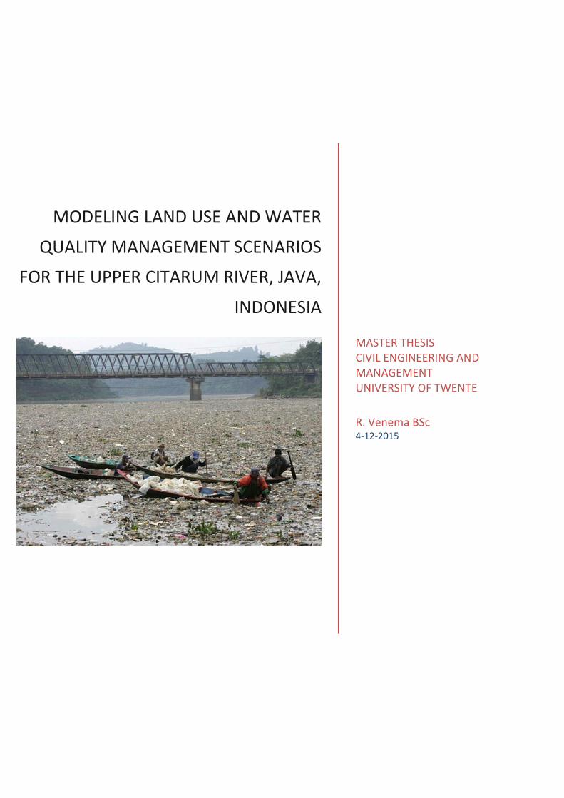
MODELING LAND USE AND WATER
QUALITY MANAGEMENT SCENARIOS
FOR THE UPPER CITARUM RIVER, JAVA,
INDONESIA
MASTER THESIS CIVIL ENGINEERING AND MANAGEMENT UNIVERSITY OF TWENTE
R. Venema BSc 4-12-2015

ii
iii
Modeling land use and water quality management scenarios for the Upper
Citarum Basin, Java, Indonesia
Master thesis In Civil Engineering and Management
Faculty of Engineering Technology University of Twente
Author Rigt Venema BSc
Contact [email protected]
Location and date Enschede, December 4,
2015
Thesis defense date December 11, 2014
Graduation Committee
Graduation Supervisor Dr. Ir. D.C.M. Augustijn University of Twente
Daily supervisor V. Harezlak MSc. University of Twente
External supervisor Dr. G.W. Geerling Radboud University Nijmegen,
Deltares
Front picture The Guardian

iv
ABSTRACT
The Citarum River is one of the most polluted rivers in the world. The main reasons for the impaired
water quality are the high population density and the rapid industrialization in the catchment.
Because of the size and variety of the problems in the Upper Citarum Basin, the high poverty levels
and an under-resourced government, the relevant institutions lack overview of how best to react
to the problems.
The goal of this research is to determine relevant scenarios and calculate the effect of these
scenarios which give stakeholders a handhold on what measures are most effective. These
scenarios are based on alternative land use and water quality management as suggested in
interviews with involved stakeholders and have the purpose to lower the concentration of pollutants
in the river compared to a reference scenario based on the current situation. The changes in
concentration for the different scenarios are modelled by a one-dimensional hydrodynamic and
water quality model (SOBEK).
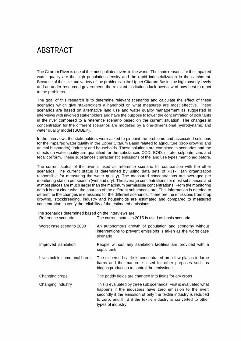
In the interviews the stakeholders were asked to pinpoint the problems and associated solutions for the impaired water quality in the Upper Citarum Basin related to agriculture (crop growing and animal husbandry), industry and households. These solutions are combined in scenarios and the effects on water quality are quantified for the substances COD, BOD, nitrate, sulphate, zinc and fecal coliform. These substances characteristic emissions of the land use types mentioned before. The current status of the river is used as reference scenario for comparison with the other scenarios. The current status is determined by using data sets of PJT-II (an organization responsible for measuring the water quality). The measured concentrations are averaged per monitoring station per season (wet and dry). The average concentrations for most substances and at most places are much larger than the maximum permissible concentrations. From the monitoring data it is not clear what the sources of the different substances are. This information is needed to determine the changes in emissions for the different scenarios. Therefore the emissions from crop growing, stockbreeding, industry and households are estimated and compared to measured concentration to verify the reliability of the estimated emissions. The scenarios determined based on the interviews are: Reference scenario The current status in 2015 is used as basis scenario
Worst case scenario 2030 An autonomous growth of population and economy without
interventions to prevent emissions is taken as the worst case
scenario
Improved sanitation People without any sanitation facilities are provided with a
septic tank
Livestock in communal barns The dispersed cattle is concentrated on a few places in large
barns and the manure is used for other purposes such as
biogas production to control the emissions
Changing crops The paddy fields are changed into fields for dry crops
Changing industry This is evaluated by three sub scenarios. First is evaluated what
happens if the industries have zero emission to the river;
secondly if the emission of only the textile industry is reduced
to zero; and third if the textile industry is converted to other
types of industry
vi
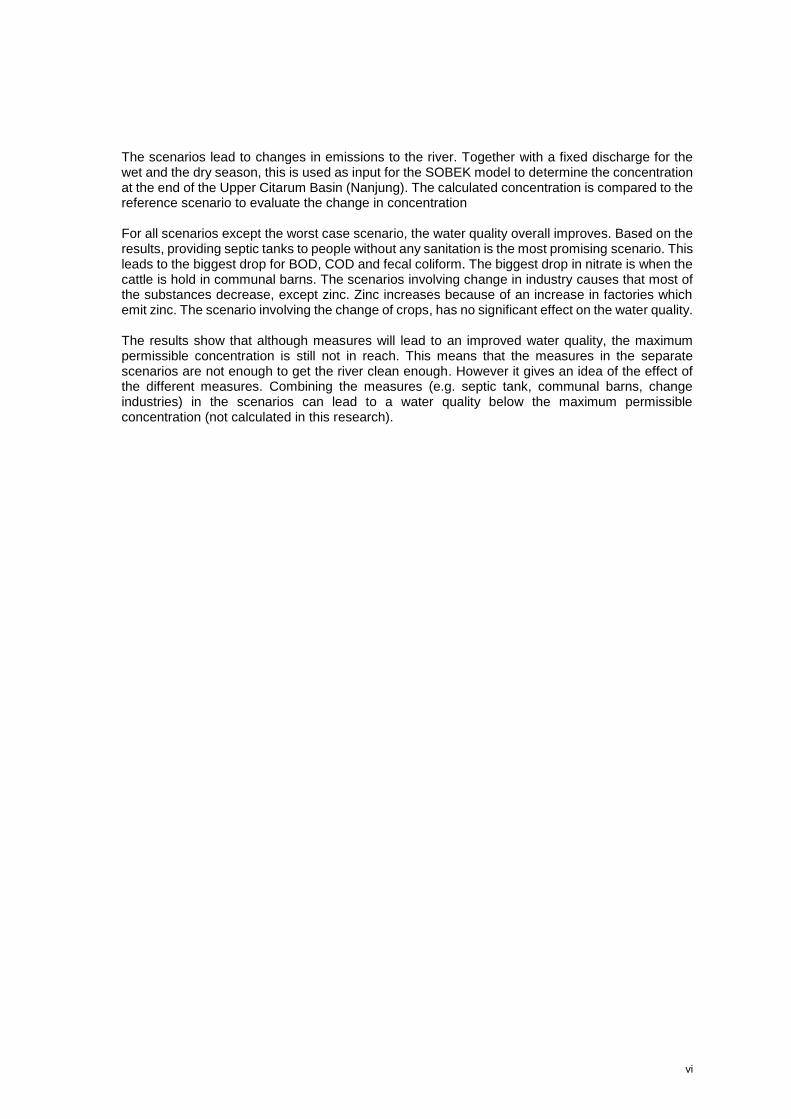
The scenarios lead to changes in emissions to the river. Together with a fixed discharge for the wet and the dry season, this is used as input for the SOBEK model to determine the concentration at the end of the Upper Citarum Basin (Nanjung). The calculated concentration is compared to the reference scenario to evaluate the change in concentration For all scenarios except the worst case scenario, the water quality overall improves. Based on the results, providing septic tanks to people without any sanitation is the most promising scenario. This leads to the biggest drop for BOD, COD and fecal coliform. The biggest drop in nitrate is when the cattle is hold in communal barns. The scenarios involving change in industry causes that most of the substances decrease, except zinc. Zinc increases because of an increase in factories which emit zinc. The scenario involving the change of crops, has no significant effect on the water quality. The results show that although measures will lead to an improved water quality, the maximum permissible concentration is still not in reach. This means that the measures in the separate scenarios are not enough to get the river clean enough. However it gives an idea of the effect of the different measures. Combining the measures (e.g. septic tank, communal barns, change industries) in the scenarios can lead to a water quality below the maximum permissible concentration (not calculated in this research).
vii
PREFACE
This documentation is the final part of my study Civil Engineering and Management at the
University of Twente. Finishing this, means finishing my period as student. This thesis tries to give
the different stakeholders a handhold how to start to improve the water quality by combining their
solutions for the water quality problems in scenarios. It is part of the PhD project of Lufiandi. I
started this graduation project in February of 2015 with a month visiting the area of interest in
Indonesia. During this month I talked with stakeholders and looked around in the area. This gave
me insights which I did not get when I stayed the whole period in The Netherlands. It also made
my project more alive for me, to see the real problems and gave me energy to finish it.
First of all, I would like to thank my supervisors for their advice and feedback: Denie Augustijn,
Valesca Harezlak, and Gertjan Geerling. Denie, thank you for your detailed feedback and guidance
during the process. You always knew to ask the questions I had not researched and by doing so
adding more depth in my research. Valesca, I want to thank you for your help with the model and
the feedback you gave. When I had questions about the model you always took the time to answer
them carefully. Gertjan I would like to thank you for the opportunity and trust you gave me to do
this research and for the arrangements you made for my stay in Indonesia. Also your enthusiasm
during our talks gave me energy to research more and go deeper into the matter.
Special thanks to Lufi and Tya. Tya, thank you very much for your help in calculating the emission
from agriculture. Lufi, I would like to thank you for your help, feedback and discussions we had
during the process. Even more I would like to thank you for the time in Indonesia. You took me out
to see Bandung, you arranged the meetings with the stakeholders and showed me the important
parts of the basin. I really appreciate that.
Furthermore I would like to thank my friends for their support, great discussions and memorable
events. I had great time at the university.
Last but not least I want to thank my family for giving me the opportunity to study and of course
their support. Pap en mam, bedankt voor alles!
Rigt Venema
Enschede, December 2015

viii
ix
CONTENTS
1 Introduction ................................................................................................................................... 10
1.1 Citarum River................................................................................................................................ 10
1.2 Study area .................................................................................................................................... 11
1.3 Land use types .............................................................................................................................. 11
1.4 Problem Definition ....................................................................................................................... 12
1.5 Research Objective and Questions ............................................................................................... 13
1.6 Research outline and methodology .............................................................................................. 14
2 Causes and their solutions in Citarum basin ................................................................................... 15
2.1 Crop growing ................................................................................................................................ 15
2.2 Animal husbandry ........................................................................................................................ 16
2.3 Domestic waste ............................................................................................................................ 17
2.4 Industry ........................................................................................................................................ 18
2.5 Overview ...................................................................................................................................... 19
3 Concentration data and river system ............................................................................................. 21
3.1 Tributaries and selection of modelled rivers ................................................................................ 21
3.2 Modelled river system .................................................................................................................. 22
3.3 Monitoring stations and organizations ........................................................................................ 23
3.4 Substances to model .................................................................................................................... 25
3.5 Measured concentration of substances ....................................................................................... 26
4 Emission determination ................................................................................................................. 30
4.1 Emission from crops ..................................................................................................................... 30
4.2 Livestock ....................................................................................................................................... 32
4.3 Domestic waste ............................................................................................................................ 34
4.4 Industry ........................................................................................................................................ 38
4.5 Overview of loads ......................................................................................................................... 43
4.6 Calculated concentrations by SOBEK............................................................................................ 46
4.7 Comparison between measured and calculated concentrations ................................................. 49
5 Scenarios ....................................................................................................................................... 51
5.1 Reference scenario ....................................................................................................................... 51
5.2 Worst case scenario 2030 ............................................................................................................ 51
x
5.3 Improved sanitation for people .................................................................................................... 53
5.4 Livestock in communal barns ....................................................................................................... 54
5.5 Changing crops ............................................................................................................................. 55
5.6 Changing Industry ........................................................................................................................ 57
6 Results Scenarios ........................................................................................................................... 61
7 Discussion ...................................................................................................................................... 64
7.1 Substances.................................................................................................................................... 64
7.2 Measured concentration data ...................................................................................................... 64
7.3 Emission determination ............................................................................................................... 64
7.4 Model ........................................................................................................................................... 66
7.5 Results .......................................................................................................................................... 67
8 Conclusions .................................................................................................................................... 68
9 Recommendations ......................................................................................................................... 70
9.1 Further research ........................................................................................................................... 70
9.2 Improving input for the model ..................................................................................................... 70
9.3 Improving the model .................................................................................................................... 70
9.4 Scenarios ...................................................................................................................................... 71
10 Bibliography ............................................................................................................................... 72
Appendix A: Quality Standards .............................................................................................................. 75
Appendix B: Formulas emission estimation agriculture and stockbreeding ........................................... 76
B.1 Agriculture .................................................................................................................................... 76
B.2 Stockbreeding .............................................................................................................................. 77
Appendix C: Tables emmission estimation agriculture and stockbreeding ............................................. 78
C.1 Estimated emission of crops to the land per sub basin ................................................................ 78
C.2 Estimated emission stockbreeding ............................................................................................... 86
Appendix D: Emission of industries ....................................................................................................... 89
D.1. Loads from industries in the original situation ................................................................................. 89
D.2. Loads from industries without textile industries ............................................................................... 90
D.3. Loads from industries with textile factories changed into other ...................................................... 91
Appendix E: Emission estimation unregistered industry ........................................................................ 92
Appendix F: Results emission estimation............................................................................................... 94

xi
10
1 INTRODUCTION
This Chapter addresses the outline of the research. First the study area and the problems will be
discussed, followed by the research questions and methodology.
1.1 Citarum River
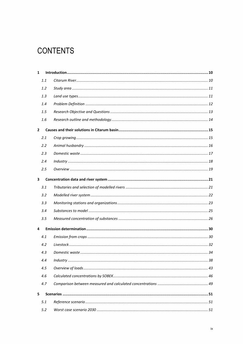
The Citarum River, 269 km long and draining an area of 12,000 km2, is one of the largest rivers on
Java (Indonesia). It originates from Mt. Wayang and flows through the middle of the western part
of the island before flowing into the Java Sea (Figure 1). The basin has an average annual rainfall
of 2300 mm, and the annual discharge at Nanjung (near the first reservoir) in the dry season is
around 30 m3/s and in the wet season a tenfold (310 m3/s). The river accommodates the need for
water of nearly 35 million people, is an important source of water for the central part of Java and
supplies 80% of the water demands of Jakarta (World Bank, 2013). The river plays a vital role in
the economic development and livelihood of the people by supporting agriculture, fisheries,
hydroelectric power generation, public water supply and industries of West Java Province and
Jakarta City (Sahu et al., 2012). It sustains 20 percent of Indonesia’s gross domestic product
(Collins, 2009). In contrast, the Citarum River is ranked by different sources as one of the most
polluted rivers in the world (Mangan, 2014). It is called the ‘Rainbow’ river because there are a lot
of textile factories on the river banks which discharge their used chemicals in the river (Groenink
& Schuurman, 2014).
FIGURE 1 LOCATION OF THE CITARUM BASIN IN INDONESIA AND THE STUDY AREA WITHIN THE BLACK CIRCLE, THIS IS UPSTREAM THE FIRST RESERVOIR
(BIG: GOOGLE MAPS, SMALL: (ADB, 2013))
11
1.2 Study area
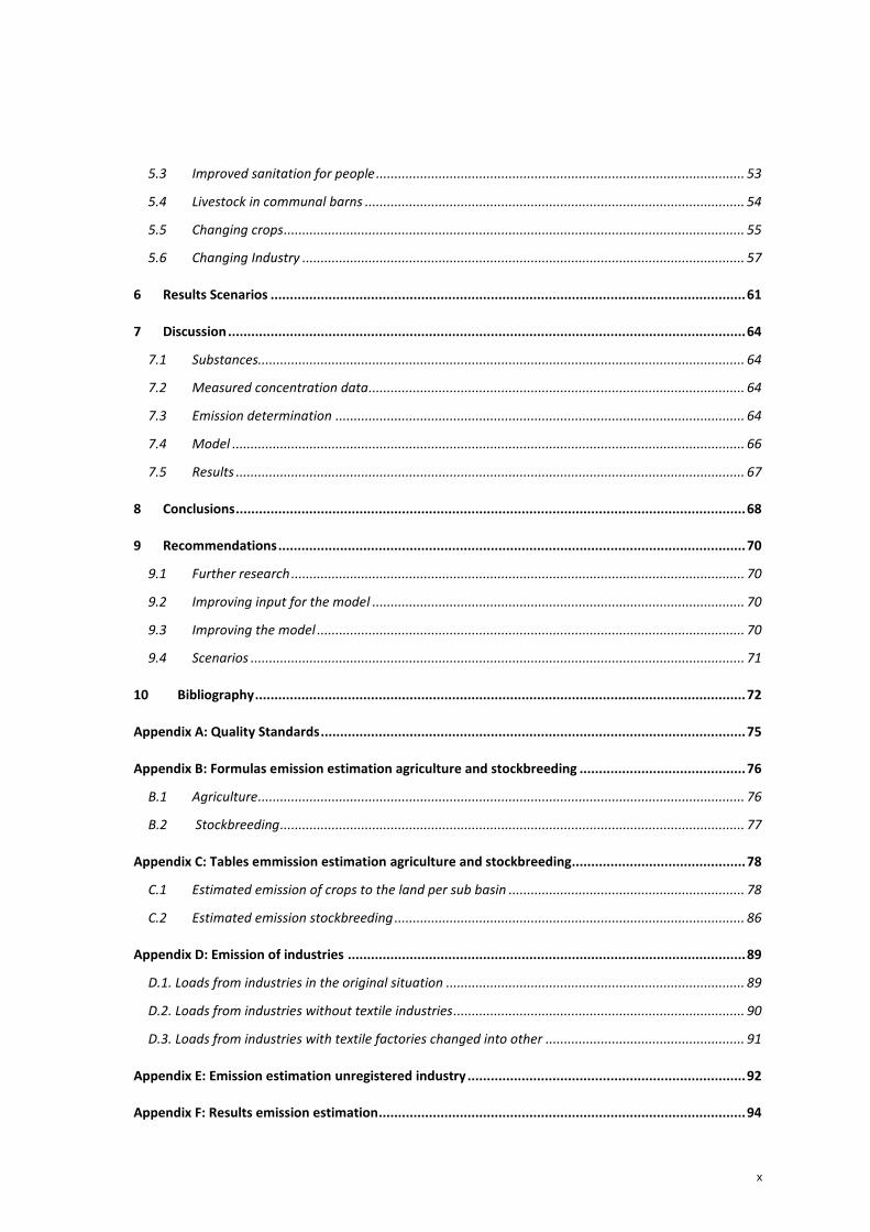
The Upper Citarum Basin is the part of the Citarum River upstream of the first reservoir (Saguling,
Figure 1). The Upper Citarum Basin is a large valley surrounded by mountains and volcanoes
(Figure 2). It lays approximately 800 meters above mean see level (Prihandrijanti & Firdayati,
2011). It contains around 20 tributaries to the Citarum River, which flow from the mountains to the
lowest part of the basin. The basin has an area of 4,800 km2 and is home to roughly eight million
people (Fares & Yudianto, 2003). The basin contains two city districts: Bandung and Cimahi.
Bandung is the third largest city of Indonesia with approximately 2.5 million inhabitants, Cimahi
has around 600,000 inhabitants.
FIGURE 2 ELEVATION MAP OF THE STUDY AREA WITH THE FIGURES IN METER ABOVE MEAN SEA LEVEL (DELTARES, 2011)
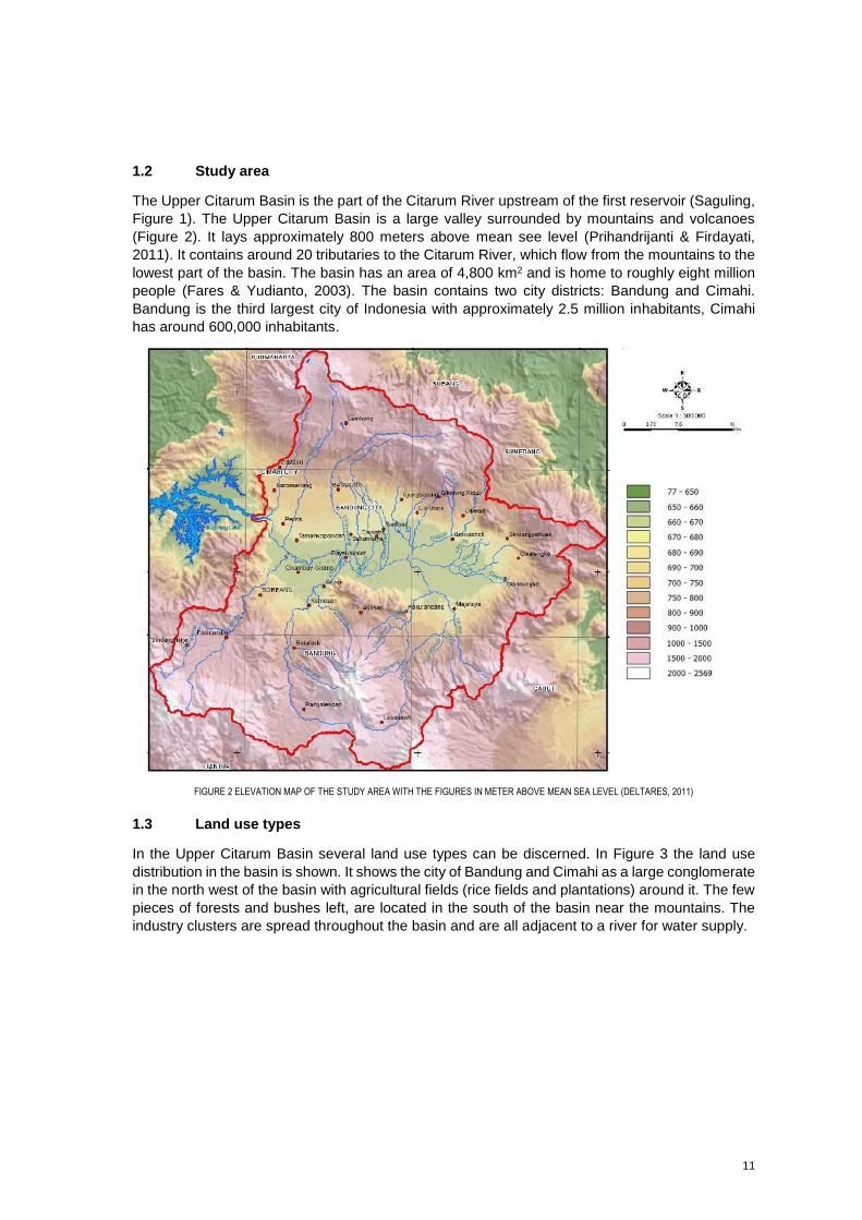
1.3 Land use types
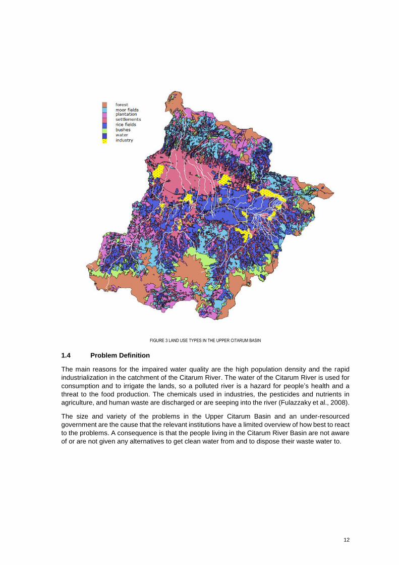
In the Upper Citarum Basin several land use types can be discerned. In Figure 3 the land use
distribution in the basin is shown. It shows the city of Bandung and Cimahi as a large conglomerate
in the north west of the basin with agricultural fields (rice fields and plantations) around it. The few
pieces of forests and bushes left, are located in the south of the basin near the mountains. The
industry clusters are spread throughout the basin and are all adjacent to a river for water supply.
12
FIGURE 3 LAND USE TYPES IN THE UPPER CITARUM BASIN
1.4 Problem Definition
The main reasons for the impaired water quality are the high population density and the rapid
industrialization in the catchment of the Citarum River. The water of the Citarum River is used for
consumption and to irrigate the lands, so a polluted river is a hazard for people’s health and a
threat to the food production. The chemicals used in industries, the pesticides and nutrients in
agriculture, and human waste are discharged or are seeping into the river (Fulazzaky et al., 2008).
The size and variety of the problems in the Upper Citarum Basin and an under-resourced
government are the cause that the relevant institutions have a limited overview of how best to react
to the problems. A consequence is that the people living in the Citarum River Basin are not aware
of or are not given any alternatives to get clean water from and to dispose their waste water to.
13
1.5 Research Objective and Questions
The problem definition leads to the following goal of this master thesis: Define alternative land use
and water quality management scenarios based on solutions suggested by stakeholders and
quantify the effect of these scenarios on the water quality. The results of this study should give the
authorities insight in which measures are most effective in improving the impaired water quality.
The objective of this research leads to the following main question:
What are possible alternative land use and water quality management scenarios and their effects
on water quality in the Upper Citarum River?
To answer this main question, some sub questions have to be answered first:
1. What are, according to the different authorities, the causes of and possible solutions for
the impaired water quality in the Upper Citarum River? (Chapter 2)
2. What are the estimated loads and resulting concentrations of the most relevant substances
to the Upper Citarum River? (Chapter 3+4)
2.1 What are the most important substances that cause the impaired water quality in the
Upper Citarum River based on water quality data? (Chapter 3)
2.2 What are the monitored concentrations of the relevant substances? (Chapter 3)
2.3 What are the loads based on estimations of emissions from different types of land
use? (Chapter 4)
2.4 How do the concentrations derived from the estimated loads compare to the measured
concentrations? (Chapter 4)
3. What are suitable scenarios for the Upper Citarum River Basin and the associated
changes in loads? (Chapter 5)
4. What are the most promising scenarios based on their effect on water quality? (Chapter
6)
14
1.6 Research outline and methodology
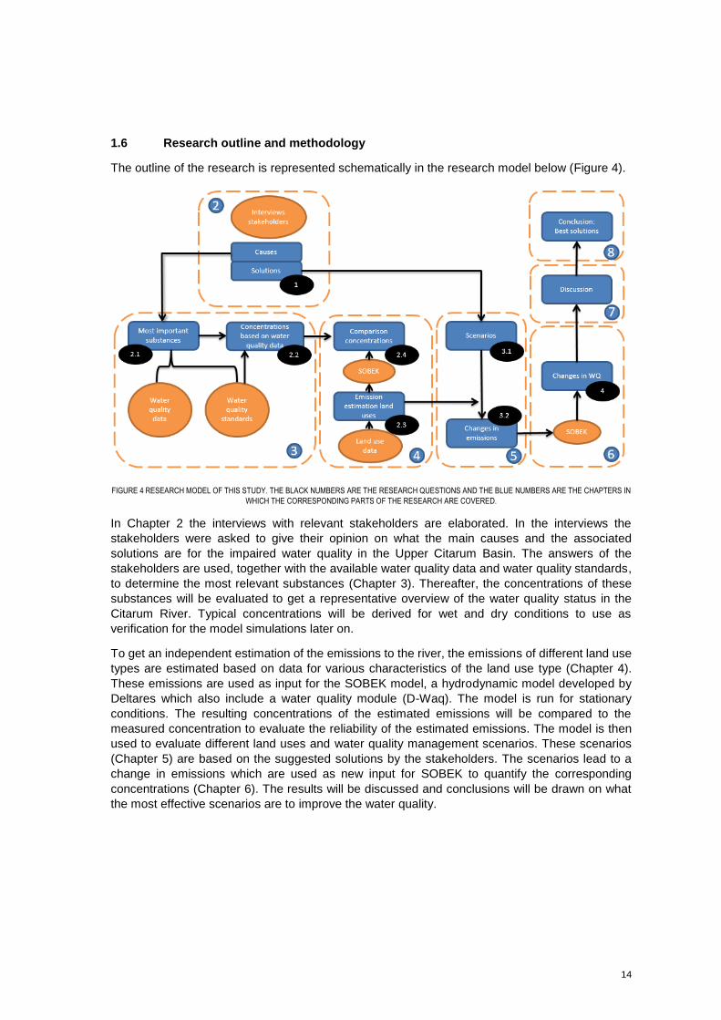
The outline of the research is represented schematically in the research model below (Figure 4).
FIGURE 4 RESEARCH MODEL OF THIS STUDY. THE BLACK NUMBERS ARE THE RESEARCH QUESTIONS AND THE BLUE NUMBERS ARE THE CHAPTERS IN
WHICH THE CORRESPONDING PARTS OF THE RESEARCH ARE COVERED.
In Chapter 2 the interviews with relevant stakeholders are elaborated. In the interviews the
stakeholders were asked to give their opinion on what the main causes and the associated
solutions are for the impaired water quality in the Upper Citarum Basin. The answers of the
stakeholders are used, together with the available water quality data and water quality standards,
to determine the most relevant substances (Chapter 3). Thereafter, the concentrations of these
substances will be evaluated to get a representative overview of the water quality status in the
Citarum River. Typical concentrations will be derived for wet and dry conditions to use as
verification for the model simulations later on.
To get an independent estimation of the emissions to the river, the emissions of different land use
types are estimated based on data for various characteristics of the land use type (Chapter 4).
These emissions are used as input for the SOBEK model, a hydrodynamic model developed by
Deltares which also include a water quality module (D-Waq). The model is run for stationary
conditions. The resulting concentrations of the estimated emissions will be compared to the
measured concentration to evaluate the reliability of the estimated emissions. The model is then
used to evaluate different land uses and water quality management scenarios. These scenarios
(Chapter 5) are based on the suggested solutions by the stakeholders. The scenarios lead to a
change in emissions which are used as new input for SOBEK to quantify the corresponding
concentrations (Chapter 6). The results will be discussed and conclusions will be drawn on what
the most effective scenarios are to improve the water quality.
15
2 CAUSES AND THEIR SOLUTIONS IN CITARUM BASIN
In this Chapter the causes of the impaired water quality in the Upper Citarum River and their
solutions are elaborated according to different stakeholders in the Upper Citarum Basin. The input
from the stakeholders is used to develop scenarios. The stakeholders interviewed were people
from the local, provincial and national government which have authority on water quality; a non-
governmental organization (NGO) which tries to raise awareness of the problem in the Citarum
River; and an organization for the water quality managers of the industry. These interviews were
held in Indonesia face to face and consisted of two questions:
1. What are the main causes of the impaired water quality per land use type?
a. Crop growing
b. Animal husbandry/stockbreeding
c. Domestic
d. Industry
2. What are the main solutions to improve the water quality per land use type?
The answers of the different stakeholders are compared and overlapping answers are combined
in scenarios. Remarkable was that stakeholders gave a lot of comparable answers, therefore no
distinction is made in the text between stakeholders.
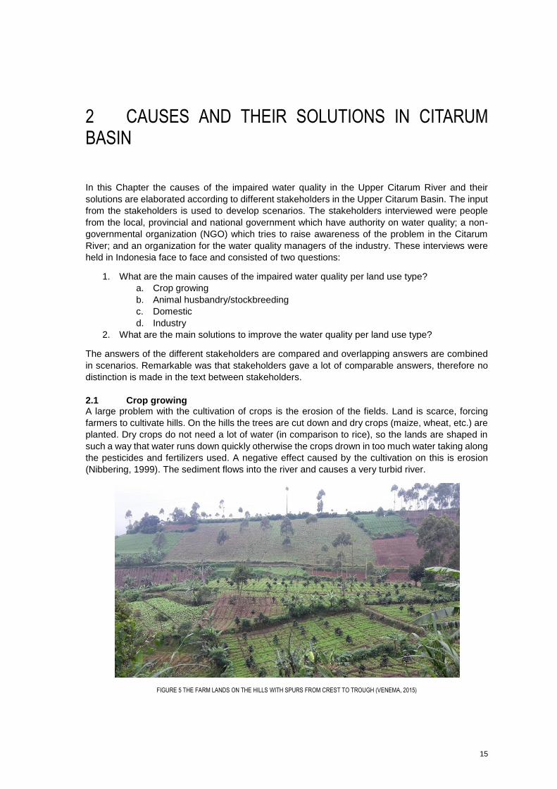
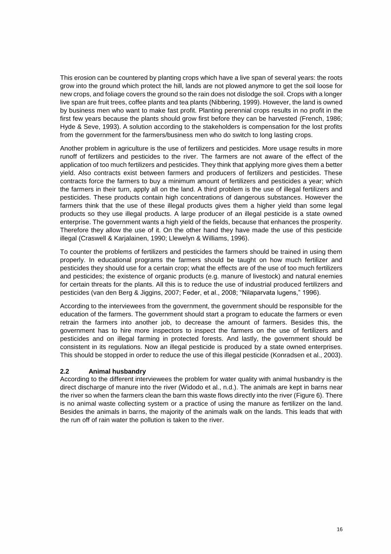
2.1 Crop growing A large problem with the cultivation of crops is the erosion of the fields. Land is scarce, forcing
farmers to cultivate hills. On the hills the trees are cut down and dry crops (maize, wheat, etc.) are
planted. Dry crops do not need a lot of water (in comparison to rice), so the lands are shaped in
such a way that water runs down quickly otherwise the crops drown in too much water taking along
the pesticides and fertilizers used. A negative effect caused by the cultivation on this is erosion
(Nibbering, 1999). The sediment flows into the river and causes a very turbid river.
FIGURE 5 THE FARM LANDS ON THE HILLS WITH SPURS FROM CREST TO TROUGH (VENEMA, 2015)
16
This erosion can be countered by planting crops which have a live span of several years: the roots
grow into the ground which protect the hill, lands are not plowed anymore to get the soil loose for
new crops, and foliage covers the ground so the rain does not dislodge the soil. Crops with a longer
live span are fruit trees, coffee plants and tea plants (Nibbering, 1999). However, the land is owned
by business men who want to make fast profit. Planting perennial crops results in no profit in the
first few years because the plants should grow first before they can be harvested (French, 1986;
Hyde & Seve, 1993). A solution according to the stakeholders is compensation for the lost profits
from the government for the farmers/business men who do switch to long lasting crops.
Another problem in agriculture is the use of fertilizers and pesticides. More usage results in more
runoff of fertilizers and pesticides to the river. The farmers are not aware of the effect of the
application of too much fertilizers and pesticides. They think that applying more gives them a better
yield. Also contracts exist between farmers and producers of fertilizers and pesticides. These
contracts force the farmers to buy a minimum amount of fertilizers and pesticides a year; which
the farmers in their turn, apply all on the land. A third problem is the use of illegal fertilizers and
pesticides. These products contain high concentrations of dangerous substances. However the
farmers think that the use of these illegal products gives them a higher yield than some legal
products so they use illegal products. A large producer of an illegal pesticide is a state owned
enterprise. The government wants a high yield of the fields, because that enhances the prosperity.
Therefore they allow the use of it. On the other hand they have made the use of this pesticide
illegal (Craswell & Karjalainen, 1990; Llewelyn & Williams, 1996).
To counter the problems of fertilizers and pesticides the farmers should be trained in using them
properly. In educational programs the farmers should be taught on how much fertilizer and
pesticides they should use for a certain crop; what the effects are of the use of too much fertilizers
and pesticides; the existence of organic products (e.g. manure of livestock) and natural enemies
for certain threats for the plants. All this is to reduce the use of industrial produced fertilizers and
pesticides (van den Berg & Jiggins, 2007; Feder, et al., 2008; “Nilaparvata lugens,” 1996).
According to the interviewees from the government, the government should be responsible for the
education of the farmers. The government should start a program to educate the farmers or even
retrain the farmers into another job, to decrease the amount of farmers. Besides this, the
government has to hire more inspectors to inspect the farmers on the use of fertilizers and
pesticides and on illegal farming in protected forests. And lastly, the government should be
consistent in its regulations. Now an illegal pesticide is produced by a state owned enterprises.
This should be stopped in order to reduce the use of this illegal pesticide (Konradsen et al., 2003).
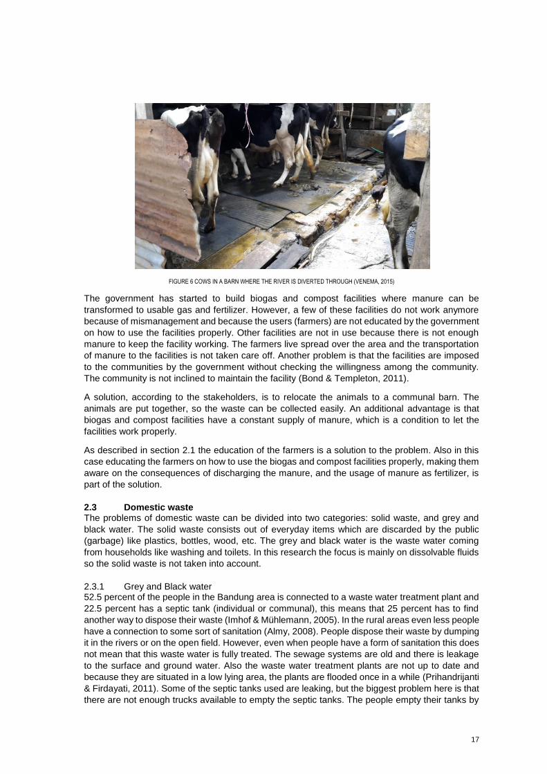
2.2 Animal husbandry According to the different interviewees the problem for water quality with animal husbandry is the
direct discharge of manure into the river (Widodo et al., n.d.). The animals are kept in barns near
the river so when the farmers clean the barn this waste flows directly into the river (Figure 6). There
is no animal waste collecting system or a practice of using the manure as fertilizer on the land.
Besides the animals in barns, the majority of the animals walk on the lands. This leads that with
the run off of rain water the pollution is taken to the river.
17
FIGURE 6 COWS IN A BARN WHERE THE RIVER IS DIVERTED THROUGH (VENEMA, 2015)
The government has started to build biogas and compost facilities where manure can be
transformed to usable gas and fertilizer. However, a few of these facilities do not work anymore
because of mismanagement and because the users (farmers) are not educated by the government
on how to use the facilities properly. Other facilities are not in use because there is not enough
manure to keep the facility working. The farmers live spread over the area and the transportation
of manure to the facilities is not taken care off. Another problem is that the facilities are imposed
to the communities by the government without checking the willingness among the community.
The community is not inclined to maintain the facility (Bond & Templeton, 2011).
A solution, according to the stakeholders, is to relocate the animals to a communal barn. The
animals are put together, so the waste can be collected easily. An additional advantage is that
biogas and compost facilities have a constant supply of manure, which is a condition to let the
facilities work properly.
As described in section 2.1 the education of the farmers is a solution to the problem. Also in this
case educating the farmers on how to use the biogas and compost facilities properly, making them
aware on the consequences of discharging the manure, and the usage of manure as fertilizer, is
part of the solution.
2.3 Domestic waste The problems of domestic waste can be divided into two categories: solid waste, and grey and
black water. The solid waste consists out of everyday items which are discarded by the public
(garbage) like plastics, bottles, wood, etc. The grey and black water is the waste water coming
from households like washing and toilets. In this research the focus is mainly on dissolvable fluids
so the solid waste is not taken into account.
2.3.1 Grey and Black water 52.5 percent of the people in the Bandung area is connected to a waste water treatment plant and
22.5 percent has a septic tank (individual or communal), this means that 25 percent has to find
another way to dispose their waste (Imhof & Mühlemann, 2005). In the rural areas even less people
have a connection to some sort of sanitation (Almy, 2008). People dispose their waste by dumping
it in the rivers or on the open field. However, even when people have a form of sanitation this does
not mean that this waste water is fully treated. The sewage systems are old and there is leakage
to the surface and ground water. Also the waste water treatment plants are not up to date and
because they are situated in a low lying area, the plants are flooded once in a while (Prihandrijanti
& Firdayati, 2011). Some of the septic tanks used are leaking, but the biggest problem here is that
there are not enough trucks available to empty the septic tanks. The people empty their tanks by
18
simply discharging it to the drainage system. Besides this, it happens that the truck drivers do not
empty their trucks at the assigned waste water treatment plants, but dump it in the river and keep
the money paid by the homeowners.
The lack of waste water treatment plants (WWTP) and septic tanks is the cause of a large part of
the problems with grey and black water. Constructing more sewage systems and WWTPs on a
community level is, according to stakeholders, the solution.
2.3.2 Overlap in domestic problems The government has a budget for collecting and processing solid waste and this same budget is
for the treatment of grey and black water. This budget is not sufficient for fully collecting and
processing both the solid and the liquid waste. The government therefore has to make a decision
in what is collected and treated. The solution is raising the budget, so the government can collect
and treat both solid waste and grey and black water.
Another problem is the development of the river banks. In the city of Bandung it is illegal to live
within ten meters of the river bank. In the rural areas this is even fifty meters. Poor people do not
have any place else to live, because of the crowded city, and therefore they build their houses in
the illegal zone near the river bank. These people do not have any sanitation facility at their
disposal because when the government facilitates a waste collecting system in these illegal areas,
the government indirectly allows the people to live there.
The solution to encounter the development of the river banks is to relocate the people elsewhere
and be strict in the enforcement of the law. By relocating the people living there the river banks are
depopulated again and by enforcing the law, people are not settling there anymore.
A lot of people are not aware of the dangers of a heavily polluted river. The government should
start a program to educate the people of the dangers of the usage of the polluted water and what
the effects are when they throw their solid waste and discharge their grey and black water into the
river.
2.4 Industry The industry can be divided into two categories: registered and unregistered. The registered
industry is registered by the government and needs to obey regulations on the maximum amount
of effluents discharged. When a company wants to register as legal industry, they have to proof
that their emissions are within standards before getting a permit. So before getting a permit, the
industry has to produce already. Therefore, there are also a large number of unregistered
industries.
2.4.1 Registered industry The registered industries are obliged to treat their water until it is within standards (Appendix A). Most of the registered industries have some sort of waste water treatment, but it costs money to run it. Therefore some managers of the industry choose to only treat the water when they expect an inspection. The rest of the time they discharge the waste water directly to the river without treatment. The water quality managers of these industries, who are responsible for the water treatment, take (according to the organization on water quality managers) a passive role and obey what the bosses tell them to do. Besides this, the technology used in the WWTPs (both owned by the industries as the communal
ones) is not advanced enough to filter all the different substances from the waste water. The
existing plants in Indonesia are for example not equipped to filter heavy metals. So even when the
water is treated, the effluent is not within standards.
The problem of the waste water treatment can be tackled by building more WWTPs and even
centralize the waste water treatment for the industry so there is more control in the quality of water
19
after treatment. Building new WWTPs gives also the opportunity to improve treatment technology
so the heavy metals are also filtered out of the waste water.
2.4.2 Unregistered industry The unregistered industries are the majority of industries in the Upper Citarum River Basin. The
West Java EPA estimates that there are 1500 industries in the basin of which 400 registered. The
unregistered industry mainly consists out of micro and small industries (home shops, little
workplaces, etc.). The unregistered industries have no permit yet or are not within standards and
thus have no rights to a permit. These industries often are hiding in communities who support the
presence of the industry because these industries provide jobs.
2.4.3 Joint problems registered and unregistered industry The monitoring whether the industries are handling within limits is taken care of by the government.
The authorities in Indonesia are unfortunately not very powerful, so the amount of inspectors to
check the industries is due to low budgets limited. Besides this, when an inspector catches an
industry in flagrante delicto, the penalties are lower than building and operating a waste water
treatment plant. Therefore the industries prefer to pay the penalties.
A solution is raising the budget, which is easier said than done, because of a poor government.
This leads to more inspectors and a better law enforcement, to force the industries to treat their
water, are necessary to improve the water quality. Higher penalties can be deterrent and a way to
enforce the rules more.
A large problem is the duality of the problem. The industry improves the employment in the country
because the rules are not that strict so foreign investors open their businesses in Indonesia. On
the other hand, when Indonesia tightens its rules, the owners of industry easily move their
companies to other countries where the rules are not that strict. This causes unemployment.
Therefore the government of Indonesia has a dilemma. A choice for the environment is a risk of
increased unemployment and a choice for employment has the risk for an increase in pollution
discharged.
Another way to give the industry a message that they have to improve their waste water treatment
is to develop a classification system for their products. For example putting an extra label inside
clothing which shows the public how polluting the manufacturer of the product is. Hopefully the
public will only choose the products which are good for the environment and in this way force the
polluting industry to treat their water properly.
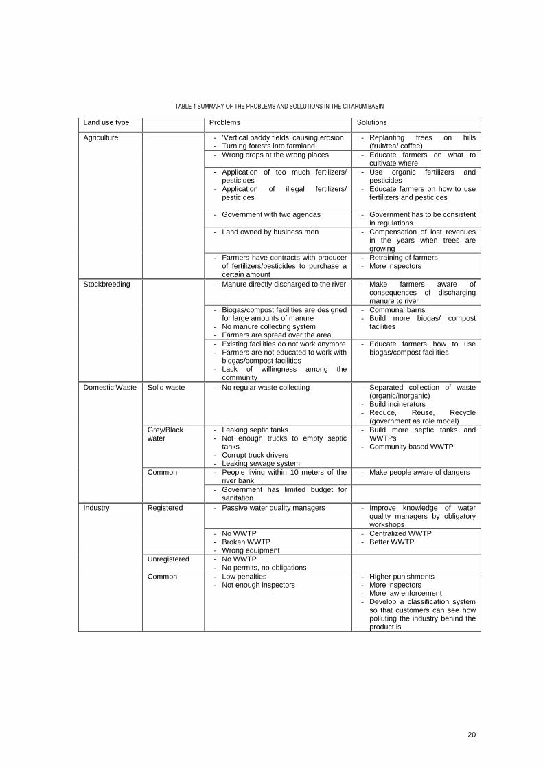
2.5 Overview
In Table 1 an overview is given of the outcome with the stakeholders. It is tried to give per problem
solutions. These are next to each other in the columns.
20
TABLE 1 SUMMARY OF THE PROBLEMS AND SOLLUTIONS IN THE CITARUM BASIN
Land use type Problems Solutions
Agriculture - ‘Vertical paddy fields’ causing erosion - Turning forests into farmland
- Replanting trees on hills (fruit/tea/ coffee)
- Wrong crops at the wrong places - Educate farmers on what to cultivate where
- Application of too much fertilizers/ pesticides
- Application of illegal fertilizers/ pesticides
- Use organic fertilizers and pesticides
- Educate farmers on how to use fertilizers and pesticides
- Government with two agendas - Government has to be consistent in regulations
- Land owned by business men - Compensation of lost revenues in the years when trees are growing
- Farmers have contracts with producer of fertilizers/pesticides to purchase a certain amount
- Retraining of farmers - More inspectors
Stockbreeding - Manure directly discharged to the river
- Make farmers aware of consequences of discharging manure to river
- Biogas/compost facilities are designed for large amounts of manure
- No manure collecting system - Farmers are spread over the area
- Communal barns - Build more biogas/ compost
facilities
- Existing facilities do not work anymore - Farmers are not educated to work with
biogas/compost facilities - Lack of willingness among the
community
- Educate farmers how to use biogas/compost facilities
Domestic Waste Solid waste - No regular waste collecting - Separated collection of waste (organic/inorganic)
- Build incinerators - Reduce, Reuse, Recycle
(government as role model)
Grey/Black water
- Leaking septic tanks - Not enough trucks to empty septic
tanks - Corrupt truck drivers - Leaking sewage system
- Build more septic tanks and WWTPs
- Community based WWTP
Common - People living within 10 meters of the river bank
- Make people aware of dangers
- Government has limited budget for sanitation
Industry Registered - Passive water quality managers - Improve knowledge of water quality managers by obligatory workshops
- No WWTP - Broken WWTP - Wrong equipment
- Centralized WWTP - Better WWTP
Unregistered - No WWTP - No permits, no obligations
Common - Low penalties - Not enough inspectors
- Higher punishments - More inspectors - More law enforcement - Develop a classification system
so that customers can see how polluting the industry behind the product is
21
3 CONCENTRATION DATA AND RIVER SYSTEM
The Citarum River is a heavily polluted river. A lot of different substances are found in the river and on its banks. Some of these substances are produced by nature but are pollutants because of the high concentration in the river. Other substances do not occur in rivers naturally and are therefore pollutants. In order to check whether the substances in the river are pollutants, the maximum permissible concentration (MPC) of substances, set by the government of the Province of West Java, is used, see Appendix A (Perda Jabar No. 39/2000). In this chapter the severity of the problem is determined with the data from organizations which
measure the concentrations in the river. To assure consistency one organization is chosen from
which the data is used. At the same time a selection is made of substances which are relevant to
review based on land use types, emissions and available data. The average concentration of these
substances are used to verify the results of the simulations in SOBEK later on.
Before determining the severity of the impaired water quality, the seasonal discharge per tributary
is described. Indonesia has namely a pronounced wet and dry season and a constant discharge
for the wet and dry season, respectively, is used in the simulations. Also in this chapter the river
system as is in SOBEK is explained.
3.1 Tributaries and selection of modelled rivers
The twenty tributaries of the Citarum River flowing through the Citarum basin are different in length
and discharge and are flowing through areas with a variety of land use types. For example, the
Citepus flows completely through the city of Bandung, while the river of Ciwidey mainly flows
through agricultural areas. This gives different concentrations of substances per tributary.
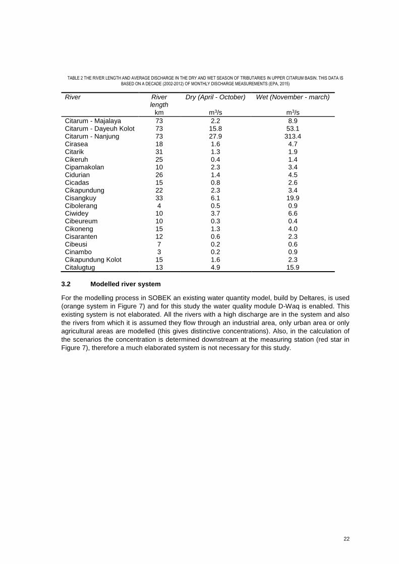
In Table 2 the length and the average discharge per season of the main tributaries and three points
in the main river are shown. The average discharge is determined by summating the discharges
measured in the months associated to the specific season and divide this by the amount of
measures. The discharges in the wet and dry season are used in the SOBEK model as fixed
discharges to calculate the concentrations. The division in wet and dry is made, because of the
run off of the different substances of the land which is higher in the wet season and because of the
higher concentration in the dry season because of less dilution.
22
TABLE 2 THE RIVER LENGTH AND AVERAGE DISCHARGE IN THE DRY AND WET SEASON OF TRIBUTARIES IN UPPER CITARUM BASIN. THIS DATA IS
BASED ON A DECADE (2002-2012) OF MONTHLY DISCHARGE MEASUREMENTS (EPA, 2015)
River River length
Dry (April - October) Wet (November - march)
km m3/s m3/s
Citarum - Majalaya 73 2.2 8.9 Citarum - Dayeuh Kolot 73 15.8 53.1 Citarum - Nanjung 73 27.9 313.4 Cirasea 18 1.6 4.7 Citarik 31 1.3 1.9 Cikeruh 25 0.4 1.4 Cipamakolan 10 2.3 3.4 Cidurian 26 1.4 4.5 Cicadas 15 0.8 2.6 Cikapundung 22 2.3 3.4 Cisangkuy 33 6.1 19.9 Cibolerang 4 0.5 0.9 Ciwidey 10 3.7 6.6 Cibeureum 10 0.3 0.4 Cikoneng 15 1.3 4.0 Cisaranten 12 0.6 2.3 Cibeusi 7 0.2 0.6 Cinambo 3 0.2 0.9 Cikapundung Kolot 15 1.6 2.3 Citalugtug 13 4.9 15.9
3.2 Modelled river system
For the modelling process in SOBEK an existing water quantity model, build by Deltares, is used
(orange system in Figure 7) and for this study the water quality module D-Waq is enabled. This
existing system is not elaborated. All the rivers with a high discharge are in the system and also
the rivers from which it is assumed they flow through an industrial area, only urban area or only
agricultural areas are modelled (this gives distinctive concentrations). Also, in the calculation of
the scenarios the concentration is determined downstream at the measuring station (red star in
Figure 7), therefore a much elaborated system is not necessary for this study.
23
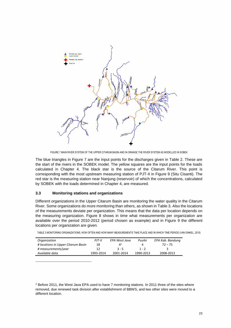
FIGURE 7 MAIN RIVER SYSTEM OF THE UPPER CITARUM BASIN AND IN ORANGE THE RIVER SYSTEM AS MODELLED IN SOBEK
The blue triangles in Figure 7 are the input points for the discharges given in Table 2. These are
the start of the rivers in the SOBEK model. The yellow squares are the input points for the loads
calculated in Chapter 4. The black star is the source of the Citarum River. This point is
corresponding with the most upstream measuring station of PJT-II in Figure 9 (Situ Cisanti). The
red star is the measuring station near Nanjung (reservoir) of which the concentrations, calculated
by SOBEK with the loads determined in Chapter 4, are measured.
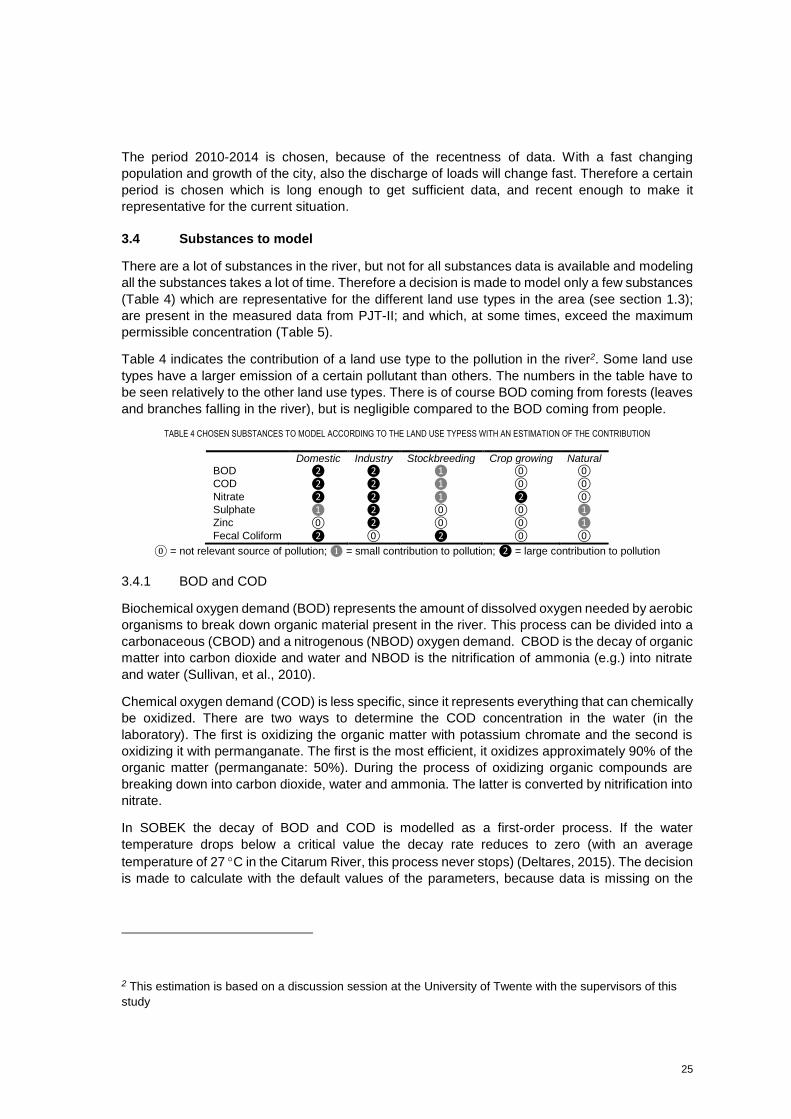
3.3 Monitoring stations and organizations
Different organizations in the Upper Citarum Basin are monitoring the water quality in the Citarum
River. Some organizations do more monitoring than others, as shown in Table 3. Also the locations
of the measurements deviate per organization. This means that the data per location depends on
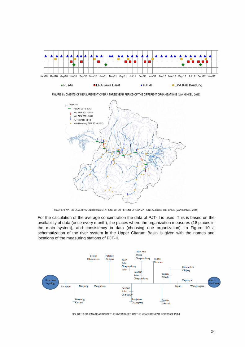
the measuring organization. Figure 8 shows in time what measurements per organization are
available over the period 2010-2012 (period chosen as example) and in Figure 9 the different
locations per organization are given.
TABLE 3 MONITORING ORGANIZATIONS, HOW OFTEN AND HOW MANY MEASUREMENTS TAKE PLACE AND IN WHICH TIME PERIOD (VAN GINKEL, 2015)
Organization PJT-II EPA West Java PusAir EPA Kab. Bandung # locations in Upper Citarum Basin 18 41 4 72 – 75 # measurements/year 12 3 - 5 1 - 2 3 Available data 1993-2014 2001-2014 1990-2013 2008-2013
1 Before 2011, the West Java EPA used to have 7 monitoring stations. In 2011 three of the sites where
removed, due renewed task division after establishment of BBWS, and two other sites were moved to a
different location.
24
FIGURE 8 MOMENTS OF MEASUREMENT OVER A THREE YEAR PERIOD OF THE DIFFERENT ORGANIZATIONS (VAN GINKEL, 2015)
FIGURE 9 WATER QUALITY MONITORING STATIONS OF DIFFERENT ORGANIZATIONS ACROSS THE BASIN (VAN GINKEL, 2015)
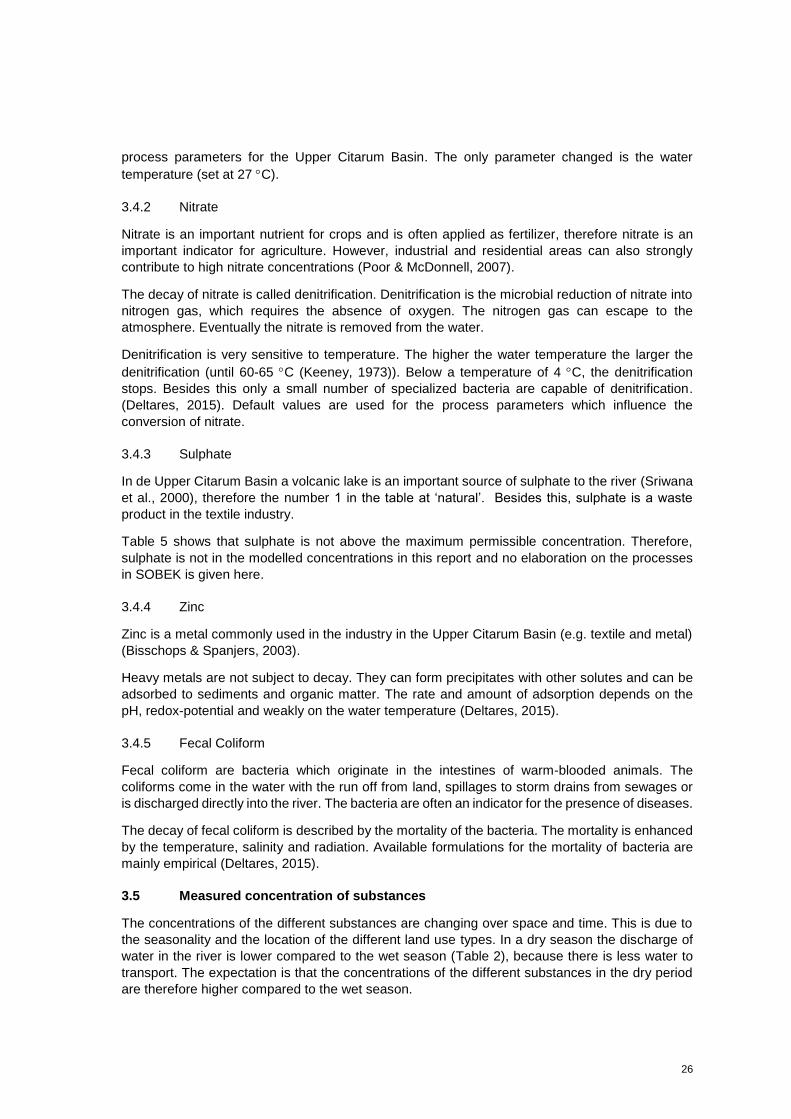
For the calculation of the average concentration the data of PJT-II is used. This is based on the
availability of data (once every month), the places where the organization measures (18 places in
the main system), and consistency in data (choosing one organization). In Figure 10 a
schematization of the river system in the Upper Citarum Basin is given with the names and
locations of the measuring stations of PJT-II.
FIGURE 10 SCHEMATISATION OF THE RIVER BASED ON THE MEASUREMENT POINTS OF PJT-II
Jan/10 Mar/10 May/10 Jul/10 Sep/10 Nov/10 Jan/11 Mar/11 May/11 Jul/11 Sep/11 Nov/11 Jan/12 Mar/12 May/12 Jul/12 Sep/12 Nov/12
PusAir EPA Jawa Barat PJT-II EPA Kab Bandung
25
The period 2010-2014 is chosen, because of the recentness of data. With a fast changing
population and growth of the city, also the discharge of loads will change fast. Therefore a certain
period is chosen which is long enough to get sufficient data, and recent enough to make it
representative for the current situation.
3.4 Substances to model
There are a lot of substances in the river, but not for all substances data is available and modeling
all the substances takes a lot of time. Therefore a decision is made to model only a few substances
(Table 4) which are representative for the different land use types in the area (see section 1.3);
are present in the measured data from PJT-II; and which, at some times, exceed the maximum
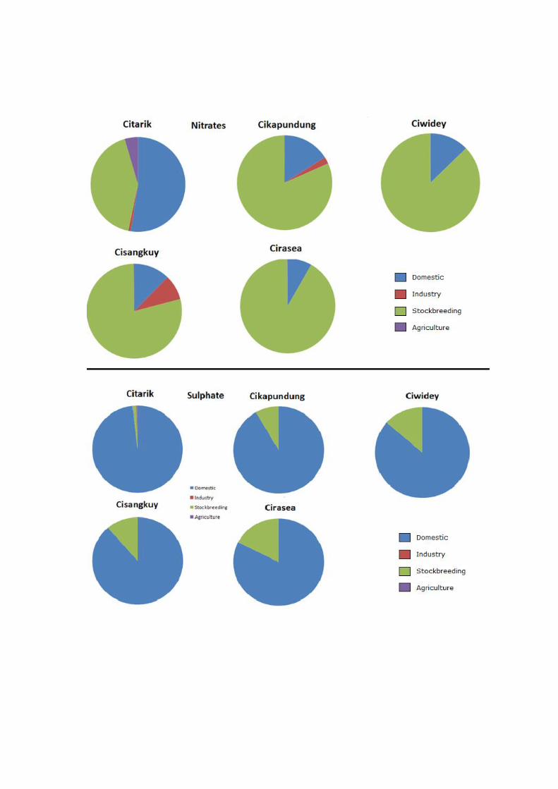
permissible concentration (Table 5).
Table 4 indicates the contribution of a land use type to the pollution in the river2. Some land use
types have a larger emission of a certain pollutant than others. The numbers in the table have to
be seen relatively to the other land use types. There is of course BOD coming from forests (leaves
and branches falling in the river), but is negligible compared to the BOD coming from people.
TABLE 4 CHOSEN SUBSTANCES TO MODEL ACCORDING TO THE LAND USE TYPESS WITH AN ESTIMATION OF THE CONTRIBUTION
Domestic Industry Stockbreeding Crop growing Natural BOD ❷ ❷ ❶ ⓪ ⓪
COD ❷ ❷ ❶ ⓪ ⓪
Nitrate ❷ ❷ ❶ ❷ ⓪
Sulphate ❶ ❷ ⓪ ⓪ ❶
Zinc ⓪ ❷ ⓪ ⓪ ❶
Fecal Coliform ❷ ⓪ ❷ ⓪ ⓪
⓪ = not relevant source of pollution; ❶ = small contribution to pollution; ❷ = large contribution to pollution
3.4.1 BOD and COD
Biochemical oxygen demand (BOD) represents the amount of dissolved oxygen needed by aerobic
organisms to break down organic material present in the river. This process can be divided into a
carbonaceous (CBOD) and a nitrogenous (NBOD) oxygen demand. CBOD is the decay of organic
matter into carbon dioxide and water and NBOD is the nitrification of ammonia (e.g.) into nitrate
and water (Sullivan, et al., 2010).
Chemical oxygen demand (COD) is less specific, since it represents everything that can chemically
be oxidized. There are two ways to determine the COD concentration in the water (in the
laboratory). The first is oxidizing the organic matter with potassium chromate and the second is
oxidizing it with permanganate. The first is the most efficient, it oxidizes approximately 90% of the
organic matter (permanganate: 50%). During the process of oxidizing organic compounds are
breaking down into carbon dioxide, water and ammonia. The latter is converted by nitrification into
nitrate.
In SOBEK the decay of BOD and COD is modelled as a first-order process. If the water
temperature drops below a critical value the decay rate reduces to zero (with an average
temperature of 27 C in the Citarum River, this process never stops) (Deltares, 2015). The decision
is made to calculate with the default values of the parameters, because data is missing on the
2 This estimation is based on a discussion session at the University of Twente with the supervisors of this
study
26
process parameters for the Upper Citarum Basin. The only parameter changed is the water
temperature (set at 27 C).
3.4.2 Nitrate
Nitrate is an important nutrient for crops and is often applied as fertilizer, therefore nitrate is an
important indicator for agriculture. However, industrial and residential areas can also strongly
contribute to high nitrate concentrations (Poor & McDonnell, 2007).
The decay of nitrate is called denitrification. Denitrification is the microbial reduction of nitrate into
nitrogen gas, which requires the absence of oxygen. The nitrogen gas can escape to the
atmosphere. Eventually the nitrate is removed from the water.
Denitrification is very sensitive to temperature. The higher the water temperature the larger the
denitrification (until 60-65 C (Keeney, 1973)). Below a temperature of 4 C, the denitrification
stops. Besides this only a small number of specialized bacteria are capable of denitrification.
(Deltares, 2015). Default values are used for the process parameters which influence the
conversion of nitrate.
3.4.3 Sulphate
In de Upper Citarum Basin a volcanic lake is an important source of sulphate to the river (Sriwana
et al., 2000), therefore the number 1 in the table at ‘natural’. Besides this, sulphate is a waste
product in the textile industry.
Table 5 shows that sulphate is not above the maximum permissible concentration. Therefore,
sulphate is not in the modelled concentrations in this report and no elaboration on the processes
in SOBEK is given here.
3.4.4 Zinc
Zinc is a metal commonly used in the industry in the Upper Citarum Basin (e.g. textile and metal)
(Bisschops & Spanjers, 2003).
Heavy metals are not subject to decay. They can form precipitates with other solutes and can be
adsorbed to sediments and organic matter. The rate and amount of adsorption depends on the
pH, redox-potential and weakly on the water temperature (Deltares, 2015).
3.4.5 Fecal Coliform
Fecal coliform are bacteria which originate in the intestines of warm-blooded animals. The
coliforms come in the water with the run off from land, spillages to storm drains from sewages or
is discharged directly into the river. The bacteria are often an indicator for the presence of diseases.
The decay of fecal coliform is described by the mortality of the bacteria. The mortality is enhanced
by the temperature, salinity and radiation. Available formulations for the mortality of bacteria are
mainly empirical (Deltares, 2015).
3.5 Measured concentration of substances
The concentrations of the different substances are changing over space and time. This is due to
the seasonality and the location of the different land use types. In a dry season the discharge of
water in the river is lower compared to the wet season (Table 2), because there is less water to
transport. The expectation is that the concentrations of the different substances in the dry period
are therefore higher compared to the wet season.
27
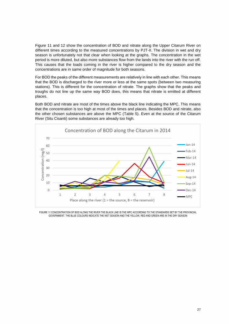
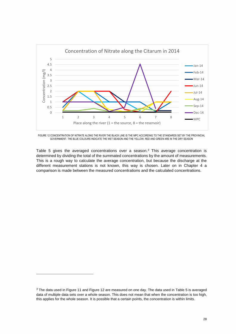
Figure 11 and 12 show the concentration of BOD and nitrate along the Upper Citarum River on
different times according to the measured concentrations by PJT-II. The division in wet and dry
season is unfortunately not that clear when looking at the graphs. The concentration in the wet
period is more diluted, but also more substances flow from the lands into the river with the run off.
This causes that the loads coming in the river is higher compared to the dry season and the
concentrations are in same order of magnitude for both seasons.
For BOD the peaks of the different measurements are relatively in line with each other. This means
that the BOD is discharged to the river more or less at the same spots (between two measuring
stations). This is different for the concentration of nitrate. The graphs show that the peaks and
troughs do not line up the same way BOD does, this means that nitrate is emitted at different
places.
Both BOD and nitrate are most of the times above the black line indicating the MPC. This means
that the concentration is too high at most of the times and places. Besides BOD and nitrate, also
the other chosen substances are above the MPC (Table 5). Even at the source of the Citarum
River (Situ Cisanti) some substances are already too high.
FIGURE 11 CONCENTRATION OF BOD ALONG THE RIVER THE BLACK LINE IS THE MPC ACCORDING TO THE STANDARDS SET BY THE PROVINCIAL
GOVERNMENT. THE BLUE COLOURS INDICATE THE WET SEASON AND THE YELLOW, RED AND GREEN ARE IN THE DRY SEASON
0
10
20
30
40
50
60
70
1 2 3 4 5 6 7 8
Co
nce
ntr
atio
n (
mg/
l)
Place along the river (1 = the source, 8 = the reservoir)
Concentration of BOD along the Citarum in 2014
Jan-14
Feb-14
Mar-14
Jun-14
Jul-14
Aug-14
Sep-14
Dec-14
MPC
28
FIGURE 12 CONCENTRATION OF NITRATE ALONG THE RIVER THE BLACK LINE IS THE MPC ACCORDING TO THE STANDARDS SET BY THE PROVINCIAL
GOVERNMENT. THE BLUE COLOURS INDICATE THE WET SEASON AND THE YELLOW, RED AND GREEN ARE IN THE DRY SEASON
Table 5 gives the averaged concentrations over a season.3 This average concentration is
determined by dividing the total of the summated concentrations by the amount of measurements.
This is a rough way to calculate the average concentration, but because the discharge at the
different measurement stations is not known, this way is chosen. Later on in Chapter 4 a
comparison is made between the measured concentrations and the calculated concentrations.
3 The data used in Figure 11 and Figure 12 are measured on one day. The data used in Table 5 is averaged
data of multiple data sets over a whole season. This does not mean that when the concentration is too high,
this applies for the whole season. It is possible that a certain points, the concentration is within limits.
0
0.5
1
1.5
2
2.5
3
3.5
4
4.5
5
1 2 3 4 5 6 7 8
Co
nce
ntr
atio
n (
mg/
l)
Place along the river (1 = the source, 8 = the reservoir)
Concentration of Nitrate along the Citarum in 2014
Jan-14
Feb-14
Mar-14
Jun-14
Jul-14
Aug-14
Sep-14
Dec-14
MPC
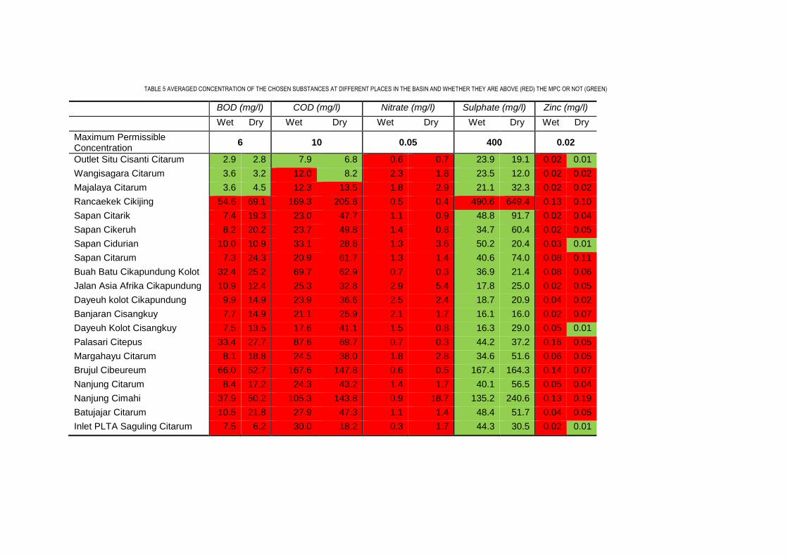
TABLE 5 AVERAGED CONCENTRATION OF THE CHOSEN SUBSTANCES AT DIFFERENT PLACES IN THE BASIN AND WHETHER THEY ARE ABOVE (RED) THE MPC OR NOT (GREEN)
BOD (mg/l) COD (mg/l) Nitrate (mg/l) Sulphate (mg/l) Zinc (mg/l)
Wet Dry Wet Dry Wet Dry Wet Dry Wet Dry
Maximum Permissible Concentration
6 10 0.05 400 0.02
Outlet Situ Cisanti Citarum 2.9 2.8 7.9 6.8 0.6 0.7 23.9 19.1 0.02 0.01
Wangisagara Citarum 3.6 3.2 12.0 8.2 2.3 1.8 23.5 12.0 0.02 0.02
Majalaya Citarum 3.6 4.5 12.3 13.5 1.8 2.9 21.1 32.3 0.02 0.02
Rancaekek Cikijing 54.6 69.1 169.3 205.8 0.5 0.4 490.6 649.4 0.13 0.10
Sapan Citarik 7.4 19.3 23.0 47.7 1.1 0.9 48.8 91.7 0.02 0.04
Sapan Cikeruh 8.2 20.2 23.7 49.8 1.4 0.8 34.7 60.4 0.02 0.05
Sapan Cidurian 10.0 10.9 33.1 28.8 1.3 3.6 50.2 20.4 0.03 0.01
Sapan Citarum 7.3 24.3 20.9 61.7 1.3 1.4 40.6 74.0 0.08 0.11
Buah Batu Cikapundung Kolot 32.4 25.2 69.7 62.9 0.7 0.3 36.9 21.4 0.08 0.06
Jalan Asia Afrika Cikapundung 10.9 12.4 25.3 32.8 2.9 5.4 17.8 25.0 0.02 0.05
Dayeuh kolot Cikapundung 9.9 14.9 23.9 36.6 2.5 2.4 18.7 20.9 0.04 0.02
Banjaran Cisangkuy 7.7 14.9 21.1 25.9 2.1 1.7 16.1 16.0 0.02 0.07
Dayeuh Kolot Cisangkuy 7.5 13.5 17.6 41.1 1.5 0.8 16.3 29.0 0.05 0.01
Palasari Citepus 33.4 27.7 87.6 69.7 0.7 0.3 44.2 37.2 0.16 0.05
Margahayu Citarum 8.1 18.8 24.5 38.0 1.8 2.8 34.6 51.6 0.06 0.05
Brujul Cibeureum 66.0 52.7 167.6 147.8 0.6 0.5 167.4 164.3 0.14 0.07
Nanjung Citarum 8.4 17.2 24.3 43.2 1.4 1.7 40.1 56.5 0.05 0.04
Nanjung Cimahi 37.9 50.2 105.3 143.8 0.9 18.7 135.2 240.6 0.13 0.19
Batujajar Citarum 10.5 21.8 27.9 47.3 1.1 1.4 48.4 51.7 0.04 0.05
Inlet PLTA Saguling Citarum 7.5 6.2 30.0 18.2 0.3 1.7 44.3 30.5 0.02 0.01
4 EMISSION DETERMINATION
In this chapter the methodology on how to estimate the loads, which are used as input for the
model, is described. This is necessary because the measurement data (section 3.5) gives no clear
answer from which land use type a particular substance originates and how much is lost by natural
processes.
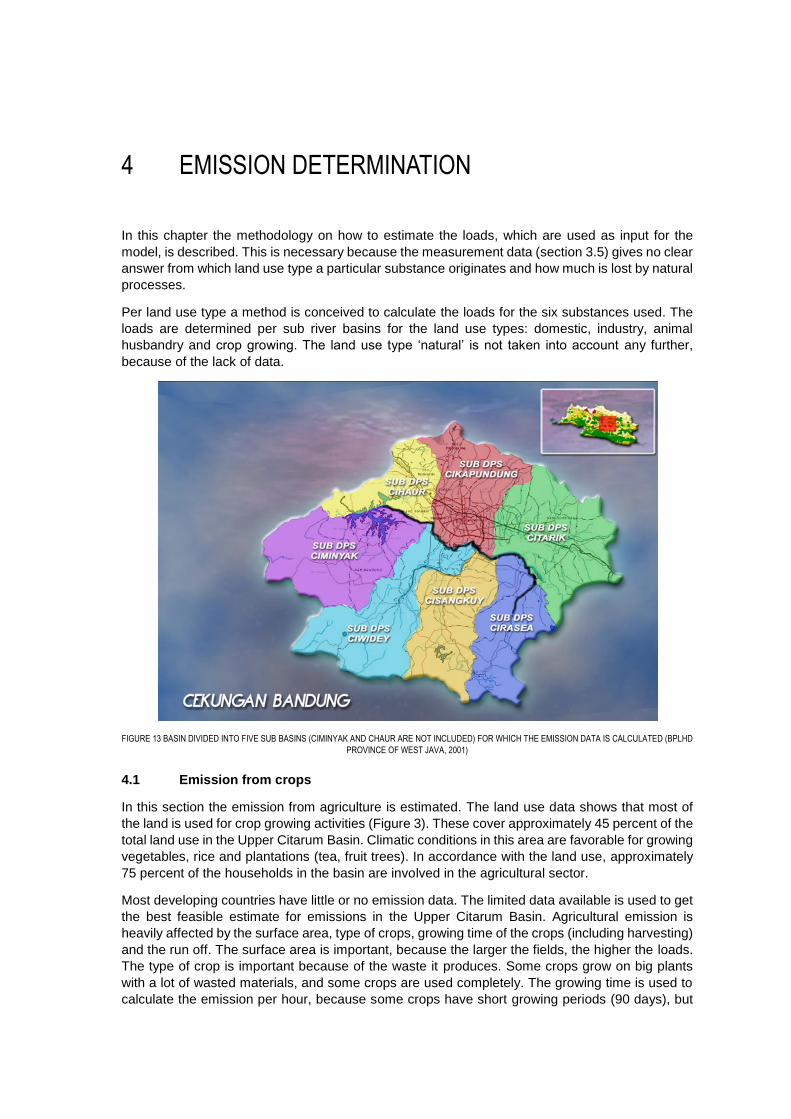
Per land use type a method is conceived to calculate the loads for the six substances used. The
loads are determined per sub river basins for the land use types: domestic, industry, animal
husbandry and crop growing. The land use type ‘natural’ is not taken into account any further,
because of the lack of data.
FIGURE 13 BASIN DIVIDED INTO FIVE SUB BASINS (CIMINYAK AND CHAUR ARE NOT INCLUDED) FOR WHICH THE EMISSION DATA IS CALCULATED (BPLHD
PROVINCE OF WEST JAVA, 2001)
4.1 Emission from crops
In this section the emission from agriculture is estimated. The land use data shows that most of
the land is used for crop growing activities (Figure 3). These cover approximately 45 percent of the
total land use in the Upper Citarum Basin. Climatic conditions in this area are favorable for growing
vegetables, rice and plantations (tea, fruit trees). In accordance with the land use, approximately
75 percent of the households in the basin are involved in the agricultural sector.
Most developing countries have little or no emission data. The limited data available is used to get
the best feasible estimate for emissions in the Upper Citarum Basin. Agricultural emission is
heavily affected by the surface area, type of crops, growing time of the crops (including harvesting)
and the run off. The surface area is important, because the larger the fields, the higher the loads.
The type of crop is important because of the waste it produces. Some crops grow on big plants
with a lot of wasted materials, and some crops are used completely. The growing time is used to
calculate the emission per hour, because some crops have short growing periods (90 days), but
31
have a large amount of emission (e.g. water spinach). The data available contains only values for
BOD, nitrate and sulphate, therefore the other substances are not taken into account in this
section.
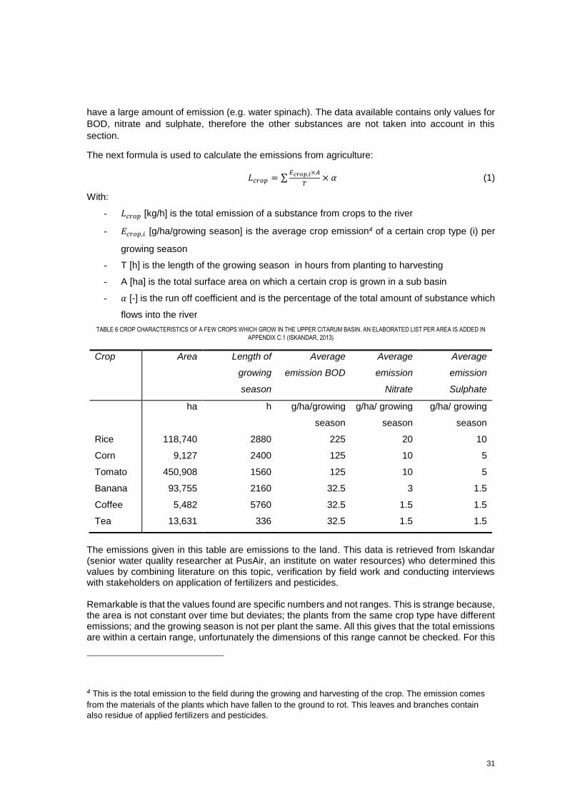
The next formula is used to calculate the emissions from agriculture:
𝐿𝑐𝑟𝑜𝑝 = ∑𝐸𝑐𝑟𝑜𝑝,𝑖×𝐴
𝑇× 𝛼 (1)
With:
- 𝐿𝑐𝑟𝑜𝑝 [kg/h] is the total emission of a substance from crops to the river
- 𝐸𝑐𝑟𝑜𝑝,𝑖 [g/ha/growing season] is the average crop emission4 of a certain crop type (i) per
growing season
- T [h] is the length of the growing season in hours from planting to harvesting
- A [ha] is the total surface area on which a certain crop is grown in a sub basin
- 𝛼 [-] is the run off coefficient and is the percentage of the total amount of substance which
flows into the river
TABLE 6 CROP CHARACTERISTICS OF A FEW CROPS WHICH GROW IN THE UPPER CITARUM BASIN. AN ELABORATED LIST PER AREA IS ADDED IN
APPENDIX C.1 (ISKANDAR, 2013)
Crop Area Length of
growing
season
Average
emission BOD
Average
emission
Nitrate
Average
emission
Sulphate
ha h g/ha/growing
season
g/ha/ growing
season
g/ha/ growing
season
Rice 118,740 2880 225 20 10
Corn 9,127 2400 125 10 5
Tomato 450,908 1560 125 10 5
Banana 93,755 2160 32.5 3 1.5
Coffee 5,482 5760 32.5 1.5 1.5
Tea 13,631 336 32.5 1.5 1.5
The emissions given in this table are emissions to the land. This data is retrieved from Iskandar (senior water quality researcher at PusAir, an institute on water resources) who determined this values by combining literature on this topic, verification by field work and conducting interviews with stakeholders on application of fertilizers and pesticides. Remarkable is that the values found are specific numbers and not ranges. This is strange because, the area is not constant over time but deviates; the plants from the same crop type have different emissions; and the growing season is not per plant the same. All this gives that the total emissions are within a certain range, unfortunately the dimensions of this range cannot be checked. For this
4 This is the total emission to the field during the growing and harvesting of the crop. The emission comes
from the materials of the plants which have fallen to the ground to rot. This leaves and branches contain
also residue of applied fertilizers and pesticides.
32
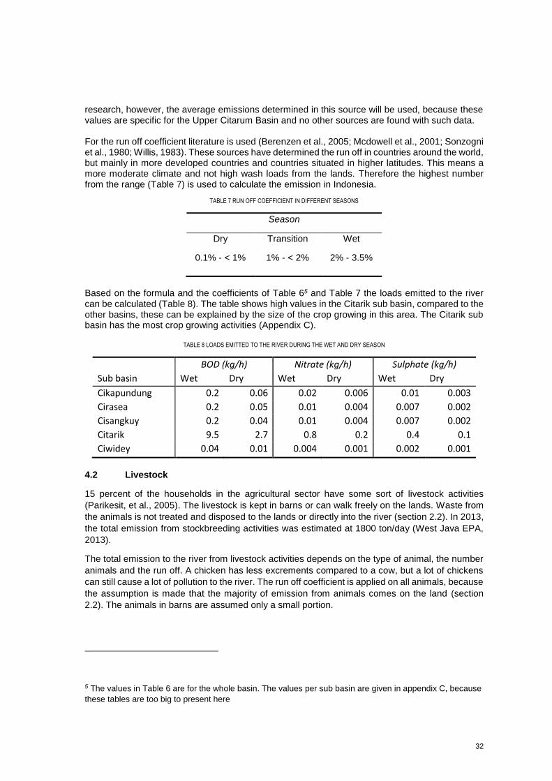
research, however, the average emissions determined in this source will be used, because these values are specific for the Upper Citarum Basin and no other sources are found with such data. For the run off coefficient literature is used (Berenzen et al., 2005; Mcdowell et al., 2001; Sonzogni et al., 1980; Willis, 1983). These sources have determined the run off in countries around the world, but mainly in more developed countries and countries situated in higher latitudes. This means a more moderate climate and not high wash loads from the lands. Therefore the highest number from the range (Table 7) is used to calculate the emission in Indonesia.
TABLE 7 RUN OFF COEFFICIENT IN DIFFERENT SEASONS
Season
Dry Transition Wet
0.1% - < 1% 1% - < 2% 2% - 3.5%
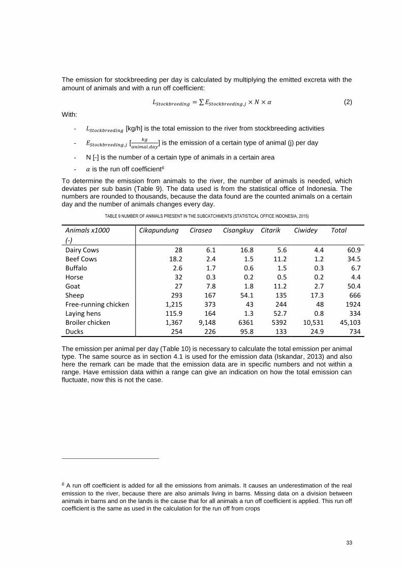
Based on the formula and the coefficients of Table 65 and Table 7 the loads emitted to the river can be calculated (Table 8). The table shows high values in the Citarik sub basin, compared to the other basins, these can be explained by the size of the crop growing in this area. The Citarik sub basin has the most crop growing activities (Appendix C).
TABLE 8 LOADS EMITTED TO THE RIVER DURING THE WET AND DRY SEASON
BOD (kg/h) Nitrate (kg/h) Sulphate (kg/h)
Sub basin Wet Dry Wet Dry Wet Dry
Cikapundung 0.2 0.06 0.02 0.006 0.01 0.003
Cirasea 0.2 0.05 0.01 0.004 0.007 0.002
Cisangkuy 0.2 0.04 0.01 0.004 0.007 0.002
Citarik 9.5 2.7 0.8 0.2 0.4 0.1
Ciwidey 0.04 0.01 0.004 0.001 0.002 0.001
4.2 Livestock
15 percent of the households in the agricultural sector have some sort of livestock activities
(Parikesit, et al., 2005). The livestock is kept in barns or can walk freely on the lands. Waste from
the animals is not treated and disposed to the lands or directly into the river (section 2.2). In 2013,
the total emission from stockbreeding activities was estimated at 1800 ton/day (West Java EPA,
2013).
The total emission to the river from livestock activities depends on the type of animal, the number
animals and the run off. A chicken has less excrements compared to a cow, but a lot of chickens
can still cause a lot of pollution to the river. The run off coefficient is applied on all animals, because
the assumption is made that the majority of emission from animals comes on the land (section
2.2). The animals in barns are assumed only a small portion.
5 The values in Table 6 are for the whole basin. The values per sub basin are given in appendix C, because
these tables are too big to present here
33
The emission for stockbreeding per day is calculated by multiplying the emitted excreta with the
amount of animals and with a run off coefficient:
𝐿𝑆𝑡𝑜𝑐𝑘𝑏𝑟𝑒𝑒𝑑𝑖𝑛𝑔 = ∑ 𝐸𝑆𝑡𝑜𝑐𝑘𝑏𝑟𝑒𝑒𝑑𝑖𝑛𝑔,𝑗 × 𝑁 × 𝛼 (2)
With:
- 𝐿𝑆𝑡𝑜𝑐𝑘𝑏𝑟𝑒𝑒𝑑𝑖𝑛𝑔 [kg/h] is the total emission to the river from stockbreeding activities
- 𝐸𝑆𝑡𝑜𝑐𝑘𝑏𝑟𝑒𝑒𝑑𝑖𝑛𝑔,𝑗 [𝑘𝑔
𝑎𝑛𝑖𝑚𝑎𝑙.𝑑𝑎𝑦] is the emission of a certain type of animal (j) per day
- N [-] is the number of a certain type of animals in a certain area
- 𝛼 is the run off coefficient6
To determine the emission from animals to the river, the number of animals is needed, which deviates per sub basin (Table 9). The data used is from the statistical office of Indonesia. The numbers are rounded to thousands, because the data found are the counted animals on a certain day and the number of animals changes every day.
TABLE 9 NUMBER OF ANIMALS PRESENT IN THE SUBCATCHMENTS (STATISTICAL OFFICE INDONESIA, 2015)
Animals x1000 Cikapundung Cirasea Cisangkuy Citarik Ciwidey Total
(-)
Dairy Cows 28 6.1 16.8 5.6 4.4 60.9 Beef Cows 18.2 2.4 1.5 11.2 1.2 34.5 Buffalo 2.6 1.7 0.6 1.5 0.3 6.7 Horse 32 0.3 0.2 0.5 0.2 4.4 Goat 27 7.8 1.8 11.2 2.7 50.4 Sheep 293 167 54.1 135 17.3 666 Free-running chicken 1,215 373 43 244 48 1924 Laying hens 115.9 164 1.3 52.7 0.8 334 Broiler chicken 1,367 9,148 6361 5392 10,531 45,103 Ducks 254 226 95.8 133 24.9 734
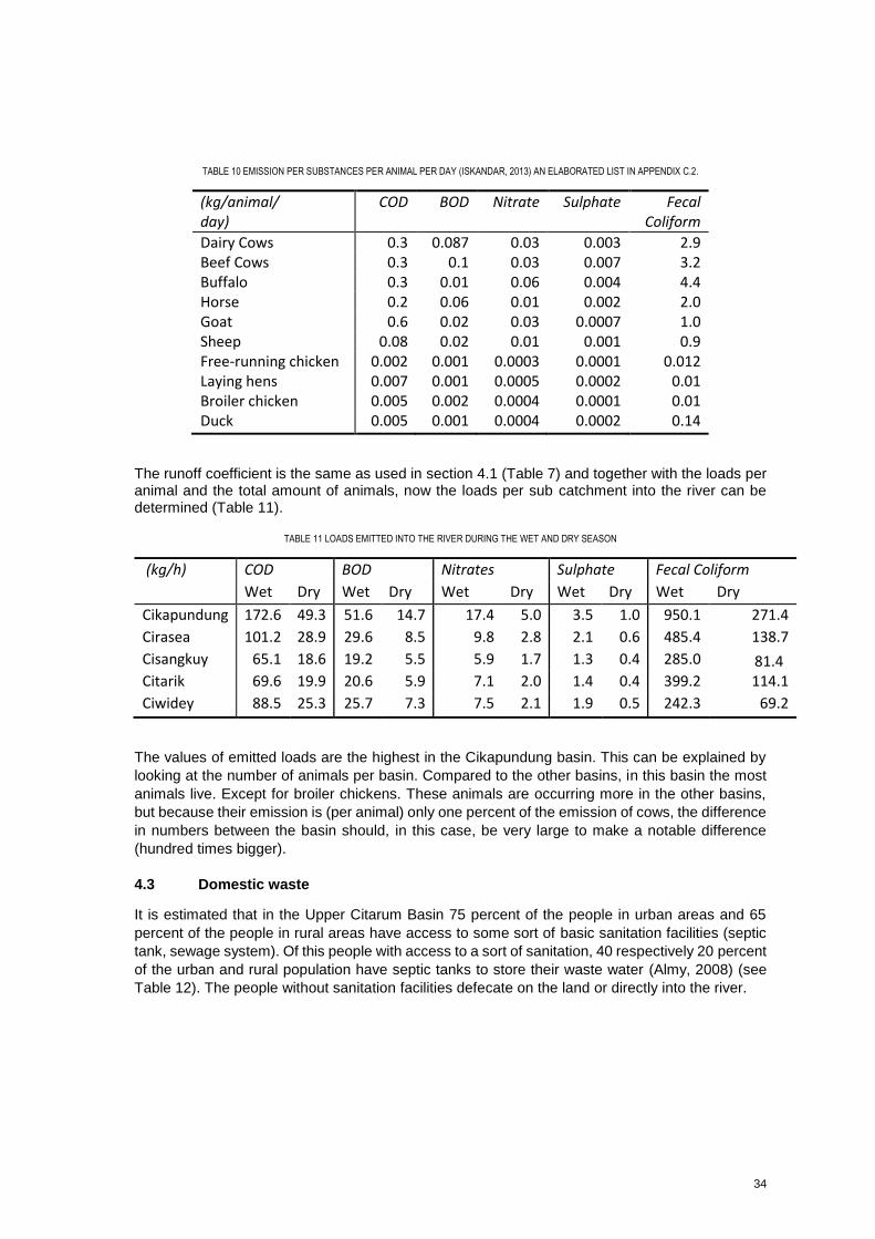
The emission per animal per day (Table 10) is necessary to calculate the total emission per animal type. The same source as in section 4.1 is used for the emission data (Iskandar, 2013) and also here the remark can be made that the emission data are in specific numbers and not within a range. Have emission data within a range can give an indication on how the total emission can fluctuate, now this is not the case.
6 A run off coefficient is added for all the emissions from animals. It causes an underestimation of the real
emission to the river, because there are also animals living in barns. Missing data on a division between
animals in barns and on the lands is the cause that for all animals a run off coefficient is applied. This run off
coefficient is the same as used in the calculation for the run off from crops
34
TABLE 10 EMISSION PER SUBSTANCES PER ANIMAL PER DAY (ISKANDAR, 2013) AN ELABORATED LIST IN APPENDIX C.2.
(kg/animal/ day)
COD BOD Nitrate Sulphate Fecal Coliform
Dairy Cows 0.3 0.087 0.03 0.003 2.9 Beef Cows 0.3 0.1 0.03 0.007 3.2 Buffalo 0.3 0.01 0.06 0.004 4.4 Horse 0.2 0.06 0.01 0.002 2.0 Goat 0.6 0.02 0.03 0.0007 1.0 Sheep 0.08 0.02 0.01 0.001 0.9 Free-running chicken 0.002 0.001 0.0003 0.0001 0.012 Laying hens 0.007 0.001 0.0005 0.0002 0.01 Broiler chicken 0.005 0.002 0.0004 0.0001 0.01 Duck 0.005 0.001 0.0004 0.0002 0.14
The runoff coefficient is the same as used in section 4.1 (Table 7) and together with the loads per animal and the total amount of animals, now the loads per sub catchment into the river can be determined (Table 11).
TABLE 11 LOADS EMITTED INTO THE RIVER DURING THE WET AND DRY SEASON
(kg/h) COD BOD Nitrates Sulphate Fecal Coliform
Wet Dry Wet Dry Wet Dry Wet Dry Wet Dry
Cikapundung 172.6 49.3 51.6 14.7 17.4 5.0 3.5 1.0 950.1 271.4
Cirasea 101.2 28.9 29.6 8.5 9.8 2.8 2.1 0.6 485.4 138.7
Cisangkuy 65.1 18.6 19.2 5.5 5.9 1.7 1.3 0.4 285.0 81.4
Citarik 69.6 19.9 20.6 5.9 7.1 2.0 1.4 0.4 399.2 114.1
Ciwidey 88.5 25.3 25.7 7.3 7.5 2.1 1.9 0.5 242.3 69.2
The values of emitted loads are the highest in the Cikapundung basin. This can be explained by
looking at the number of animals per basin. Compared to the other basins, in this basin the most
animals live. Except for broiler chickens. These animals are occurring more in the other basins,
but because their emission is (per animal) only one percent of the emission of cows, the difference
in numbers between the basin should, in this case, be very large to make a notable difference
(hundred times bigger).
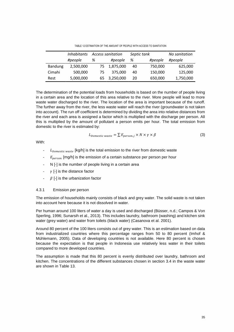
4.3 Domestic waste
It is estimated that in the Upper Citarum Basin 75 percent of the people in urban areas and 65
percent of the people in rural areas have access to some sort of basic sanitation facilities (septic
tank, sewage system). Of this people with access to a sort of sanitation, 40 respectively 20 percent
of the urban and rural population have septic tanks to store their waste water (Almy, 2008) (see
Table 12). The people without sanitation facilities defecate on the land or directly into the river.
35
TABLE 12 ESTIMATION OF THE AMOUNT OF PEOPLE WITH ACCESS TO SANITATION
Inhabitants Access sanitation Septic tank No sanitation
#people % #people % #people #people
Bandung 2,500,000 75 1,875,000 40 750,000 625,000
Cimahi 500,000 75 375,000 40 150,000 125,000
Rest 5,000,000 65 3,250,000 20 650,000 1,750,000
The determination of the potential loads from households is based on the number of people living
in a certain area and the location of this area relative to the river. More people will lead to more
waste water discharged to the river. The location of the area is important because of the runoff.
The further away from the river, the less waste water will reach the river (groundwater is not taken
into account). The run off coefficient is determined by dividing the area into relative distances from
the river and each area is assigned a factor which is multiplied with the discharge per person. All
this is multiplied by the amount of pollutant a person emits per hour. The total emission from
domestic to the river is estimated by:
𝐿𝐷𝑜𝑚𝑒𝑠𝑡𝑖𝑐 𝑤𝑎𝑠𝑡𝑒 = ∑ 𝐸𝑝𝑒𝑟𝑠𝑜𝑛,𝑗 × 𝑁 × 𝛾 × 𝛽 (3)
With:
- 𝐿𝐷𝑜𝑚𝑒𝑠𝑡𝑖𝑐 𝑤𝑎𝑠𝑡𝑒 [kg/h] is the total emission to the river from domestic waste
- 𝐸𝑝𝑒𝑟𝑠𝑜𝑛 [mg/h] is the emission of a certain substance per person per hour
- N [-] is the number of people living in a certain area
- 𝛾 [-] is the distance factor
- 𝛽 [-] is the urbanization factor
4.3.1 Emission per person
The emission of households mainly consists of black and grey water. The solid waste is not taken
into account here because it is not dissolved in water.
Per human around 100 liters of water a day is used and discharged (Büsser, n.d.; Campos & Von
Sperling, 1996; Sunarsih et al., 2013). This includes laundry, bathroom (washing) and kitchen sink
water (grey water) and water from toilets (black water) (Casanova et al. 2001).
Around 80 percent of the 100 liters consists out of grey water. This is an estimation based on data
from industrialized countries where this percentage ranges from 50 to 80 percent (Imhof &
Mühlemann, 2005). Data of developing countries is not available. Here 80 percent is chosen
because the expectation is that people in Indonesia use relatively less water in their toilets
compared to more developed countries.
The assumption is made that this 80 percent is evenly distributed over laundry, bathroom and
kitchen. The concentrations of the different substances chosen in section 3.4 in the waste water
are shown in Table 13.
36
TABLE 13 CONCENTRATIONS FOR DOMESTIC DISCHARGE IN MILLIGRAM PER LITER (A: ALMY, 2008; B: ASSESSMENT & QUALITY, 2013; C: IMHOF &
MÜHLEMANN, 2005)7
COD (mg/l)
BOD (mg/l)
Nitrate (mg/l)
Sulphate (mg/l)
Fecal Coliform (bacteria/l)
Laundry 375C 150C 0.5C - - Bathroom 1000C 170 2.5C 25 - Kitchen sink 1000C 600C - - - Toilet 610A, B 220A, B 0A, B 20A, B 300000A, B
In the literature used to determine the concentrations of the different substances in the household
waste water, some anomalies are found. The concentrations of COD and BOD in the waste water
from bathroom and kitchen sink are very high compared to the waste water from the toilet. For
COD the reason is that also the household chemicals like soap and detergent are included. The
high levels of BOD are assumed to be caused by the food waste flushed through the sink. The
absence of nitrate in the waste water from toilets is because the human body converts nitrate into
nitrite before it is emitted in the urine.
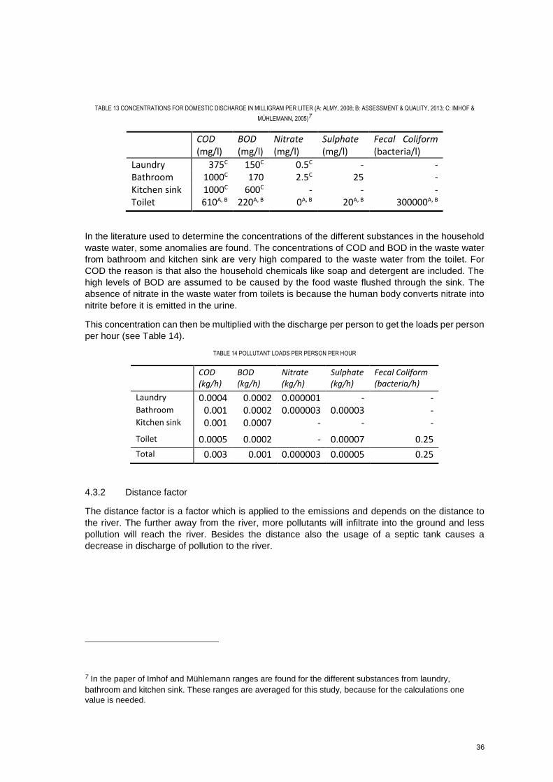
This concentration can then be multiplied with the discharge per person to get the loads per person
per hour (see Table 14).
TABLE 14 POLLUTANT LOADS PER PERSON PER HOUR
COD (kg/h)
BOD (kg/h)
Nitrate (kg/h)
Sulphate (kg/h)
Fecal Coliform (bacteria/h)
Laundry 0.0004 0.0002 0.000001 - - Bathroom 0.001 0.0002 0.000003 0.00003 - Kitchen sink 0.001 0.0007 - - -
Toilet 0.0005 0.0002 - 0.00007 0.25
Total 0.003 0.001 0.000003 0.00005 0.25
4.3.2 Distance factor
The distance factor is a factor which is applied to the emissions and depends on the distance to
the river. The further away from the river, more pollutants will infiltrate into the ground and less
pollution will reach the river. Besides the distance also the usage of a septic tank causes a
decrease in discharge of pollution to the river.
7 In the paper of Imhof and Mühlemann ranges are found for the different substances from laundry,
bathroom and kitchen sink. These ranges are averaged for this study, because for the calculations one
value is needed.
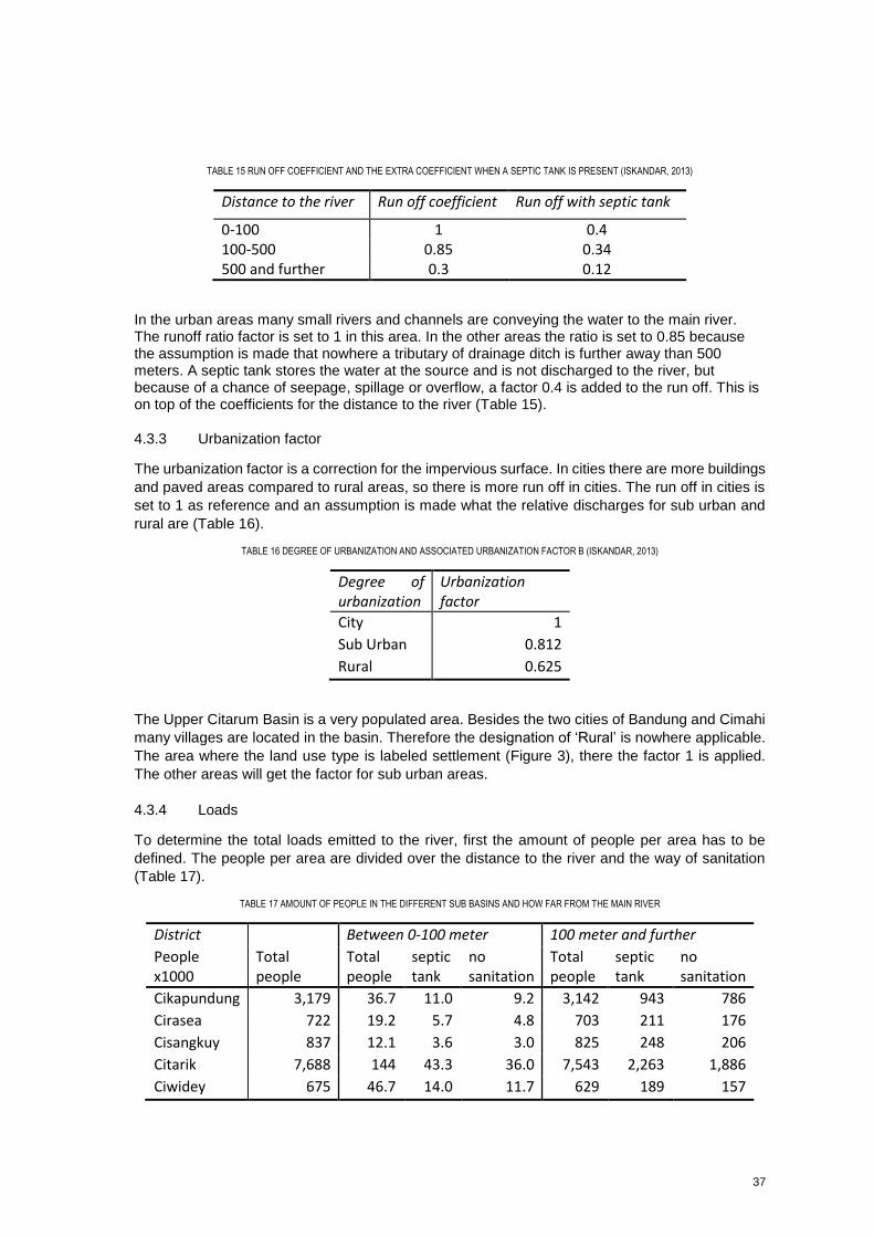
37
TABLE 15 RUN OFF COEFFICIENT AND THE EXTRA COEFFICIENT WHEN A SEPTIC TANK IS PRESENT (ISKANDAR, 2013)
Distance to the river Run off coefficient Run off with septic tank
0-100 1 0.4 100-500 0.85 0.34 500 and further 0.3 0.12
In the urban areas many small rivers and channels are conveying the water to the main river. The runoff ratio factor is set to 1 in this area. In the other areas the ratio is set to 0.85 because the assumption is made that nowhere a tributary of drainage ditch is further away than 500 meters. A septic tank stores the water at the source and is not discharged to the river, but because of a chance of seepage, spillage or overflow, a factor 0.4 is added to the run off. This is on top of the coefficients for the distance to the river (Table 15).
4.3.3 Urbanization factor
The urbanization factor is a correction for the impervious surface. In cities there are more buildings
and paved areas compared to rural areas, so there is more run off in cities. The run off in cities is
set to 1 as reference and an assumption is made what the relative discharges for sub urban and
rural are (Table 16).
TABLE 16 DEGREE OF URBANIZATION AND ASSOCIATED URBANIZATION FACTOR Β (ISKANDAR, 2013)
Degree of urbanization
Urbanization factor
City 1
Sub Urban 0.812
Rural 0.625
The Upper Citarum Basin is a very populated area. Besides the two cities of Bandung and Cimahi
many villages are located in the basin. Therefore the designation of ‘Rural’ is nowhere applicable.
The area where the land use type is labeled settlement (Figure 3), there the factor 1 is applied.
The other areas will get the factor for sub urban areas.
4.3.4 Loads
To determine the total loads emitted to the river, first the amount of people per area has to be
defined. The people per area are divided over the distance to the river and the way of sanitation
(Table 17).
TABLE 17 AMOUNT OF PEOPLE IN THE DIFFERENT SUB BASINS AND HOW FAR FROM THE MAIN RIVER
District Between 0-100 meter 100 meter and further
People x1000
Total people
Total people
septic tank
no sanitation
Total people
septic tank
no sanitation
Cikapundung 3,179 36.7 11.0 9.2 3,142 943 786
Cirasea 722 19.2 5.7 4.8 703 211 176
Cisangkuy 837 12.1 3.6 3.0 825 248 206
Citarik 7,688 144 43.3 36.0 7,543 2,263 1,886
Ciwidey 675 46.7 14.0 11.7 629 189 157
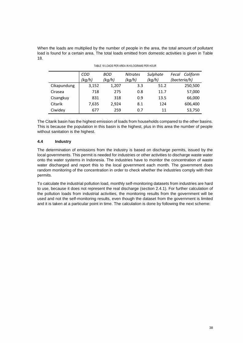
38
When the loads are multiplied by the number of people in the area, the total amount of pollutant
load is found for a certain area. The total loads emitted from domestic activities is given in Table
18.
TABLE 18 LOADS PER AREA IN KILOGRAMS PER HOUR
COD (kg/h)
BOD (kg/h)
Nitrates (kg/h)
Sulphate (kg/h)
Fecal Coliform (bacteria/h)
Cikapundung 3,152 1,207 3.3 51.2 250,500
Cirasea 718 275 0.8 11.7 57,000
Cisangkuy 831 318 0.9 13.5 66,000
Citarik 7,635 2,924 8.1 124 606,400
Ciwidey 677 259 0.7 11 53,750
The Citarik basin has the highest emission of loads from households compared to the other basins.
This is because the population in this basin is the highest, plus in this area the number of people
without sanitation is the highest.
4.4 Industry
The determination of emissions from the industry is based on discharge permits, issued by the
local governments. This permit is needed for industries or other activities to discharge waste water
onto the water systems in Indonesia. The industries have to monitor the concentration of waste
water discharged and report this to the local government each month. The government does
random monitoring of the concentration in order to check whether the industries comply with their
permits.
To calculate the industrial pollution load, monthly self-monitoring datasets from industries are hard
to use, because it does not represent the real discharge (section 2.4.1). For further calculation of
the pollution loads from industrial activities, the monitoring results from the government will be
used and not the self-monitoring results, even though the dataset from the government is limited
and it is taken at a particular point in time. The calculation is done by following the next scheme:
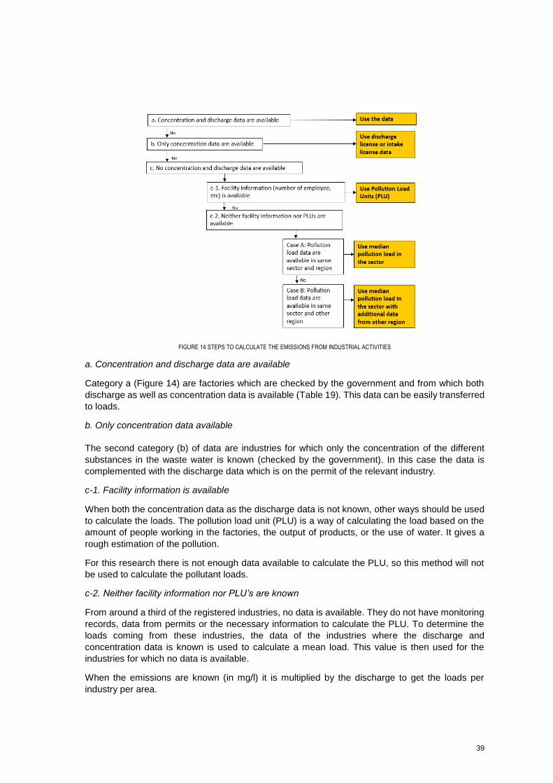
39
FIGURE 14 STEPS TO CALCULATE THE EMISSIONS FROM INDUSTRIAL ACTIVITIES
a. Concentration and discharge data are available
Category a (Figure 14) are factories which are checked by the government and from which both
discharge as well as concentration data is available (Table 19). This data can be easily transferred
to loads.
b. Only concentration data available
The second category (b) of data are industries for which only the concentration of the different
substances in the waste water is known (checked by the government). In this case the data is
complemented with the discharge data which is on the permit of the relevant industry.
c-1. Facility information is available
When both the concentration data as the discharge data is not known, other ways should be used
to calculate the loads. The pollution load unit (PLU) is a way of calculating the load based on the
amount of people working in the factories, the output of products, or the use of water. It gives a
rough estimation of the pollution.
For this research there is not enough data available to calculate the PLU, so this method will not
be used to calculate the pollutant loads.
c-2. Neither facility information nor PLU’s are known
From around a third of the registered industries, no data is available. They do not have monitoring
records, data from permits or the necessary information to calculate the PLU. To determine the
loads coming from these industries, the data of the industries where the discharge and
concentration data is known is used to calculate a mean load. This value is then used for the
industries for which no data is available.
When the emissions are known (in mg/l) it is multiplied by the discharge to get the loads per
industry per area.
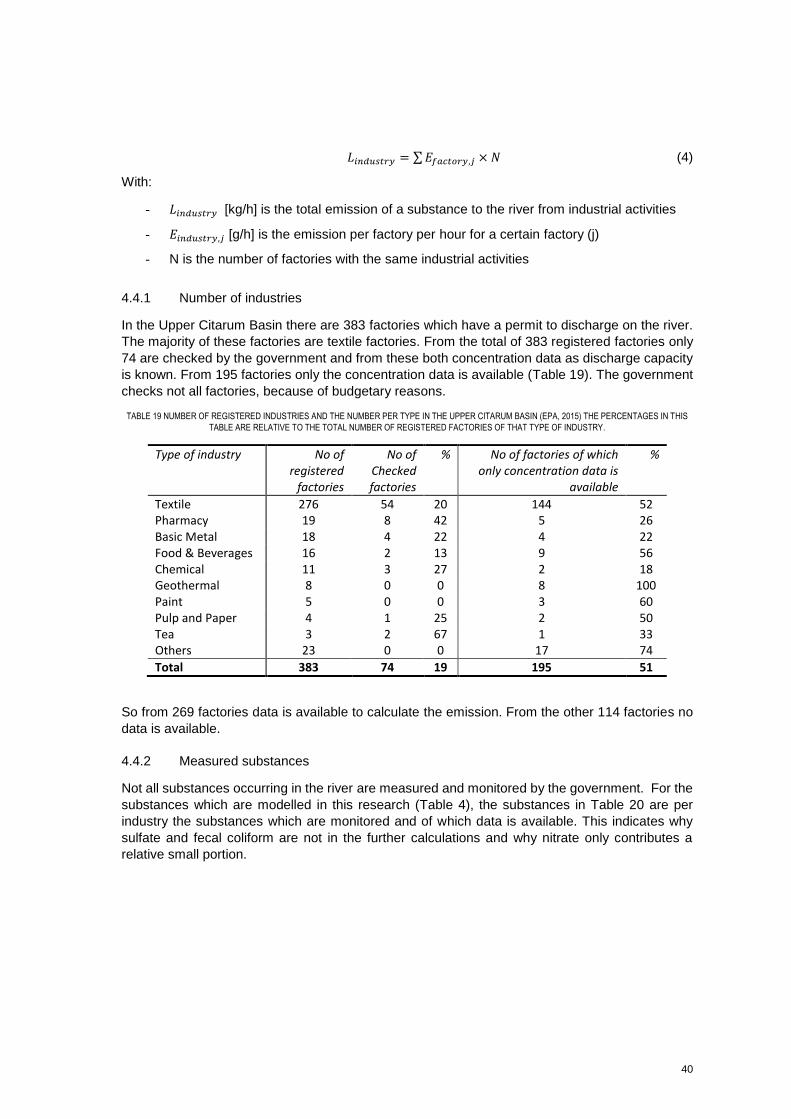
40
𝐿𝑖𝑛𝑑𝑢𝑠𝑡𝑟𝑦 = ∑ 𝐸𝑓𝑎𝑐𝑡𝑜𝑟𝑦,𝑗 × 𝑁 (4)
With:
- 𝐿𝑖𝑛𝑑𝑢𝑠𝑡𝑟𝑦 [kg/h] is the total emission of a substance to the river from industrial activities
- 𝐸𝑖𝑛𝑑𝑢𝑠𝑡𝑟𝑦,𝑗 [g/h] is the emission per factory per hour for a certain factory (j)
- N is the number of factories with the same industrial activities
4.4.1 Number of industries
In the Upper Citarum Basin there are 383 factories which have a permit to discharge on the river.
The majority of these factories are textile factories. From the total of 383 registered factories only
74 are checked by the government and from these both concentration data as discharge capacity
is known. From 195 factories only the concentration data is available (Table 19). The government
checks not all factories, because of budgetary reasons.
TABLE 19 NUMBER OF REGISTERED INDUSTRIES AND THE NUMBER PER TYPE IN THE UPPER CITARUM BASIN (EPA, 2015) THE PERCENTAGES IN THIS
TABLE ARE RELATIVE TO THE TOTAL NUMBER OF REGISTERED FACTORIES OF THAT TYPE OF INDUSTRY.
Type of industry No of registered
factories
No of Checked
factories
% No of factories of which only concentration data is
available
%
Textile 276 54 20 144 52 Pharmacy 19 8 42 5 26 Basic Metal 18 4 22 4 22 Food & Beverages 16 2 13 9 56 Chemical 11 3 27 2 18 Geothermal 8 0 0 8 100 Paint 5 0 0 3 60 Pulp and Paper 4 1 25 2 50 Tea 3 2 67 1 33 Others 23 0 0 17 74
Total 383 74 19 195 51
So from 269 factories data is available to calculate the emission. From the other 114 factories no
data is available.
4.4.2 Measured substances
Not all substances occurring in the river are measured and monitored by the government. For the
substances which are modelled in this research (Table 4), the substances in Table 20 are per
industry the substances which are monitored and of which data is available. This indicates why
sulfate and fecal coliform are not in the further calculations and why nitrate only contributes a
relative small portion.
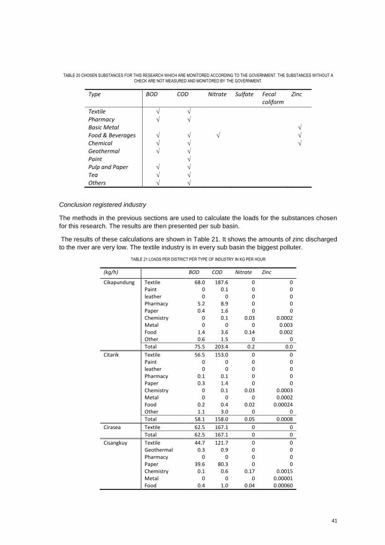
41
TABLE 20 CHOSEN SUBSTANCES FOR THIS RESEARCH WHICH ARE MONITORED ACCORDING TO THE GOVERNMENT. THE SUBSTANCES WITHOUT A
CHECK ARE NOT MEASURED AND MONITORED BY THE GOVERNMENT.
Type BOD COD Nitrate Sulfate Fecal coliform
Zinc
Textile Pharmacy Basic Metal
Food & Beverages
Chemical
Geothermal Paint Pulp and Paper Tea Others
Conclusion registered industry
The methods in the previous sections are used to calculate the loads for the substances chosen
for this research. The results are then presented per sub basin.
The results of these calculations are shown in Table 21. It shows the amounts of zinc discharged
to the river are very low. The textile industry is in every sub basin the biggest polluter.
TABLE 21 LOADS PER DISTRICT PER TYPE OF INDUSTRY IN KG PER HOUR
(kg/h) BOD COD Nitrate Zinc
Cikapundung Textile 68.0 187.6 0 0 Paint 0 0.1 0 0 leather 0 0 0 0 Pharmacy 5.2 8.9 0 0 Paper 0.4 1.6 0 0 Chemistry 0 0.1 0.03 0.0002 Metal 0 0 0 0.003 Food 1.4 3.6 0.14 0.002 Other 0.6 1.5 0 0
Total 75.5 203.4 0.2 0.0
Citarik Textile 56.5 153.0 0 0 Paint 0 0 0 0 leather 0 0 0 0 Pharmacy 0.1 0.1 0 0 Paper 0.3 1.4 0 0 Chemistry 0 0.1 0.03 0.0003 Metal 0 0 0 0.0002 Food 0.2 0.4 0.02 0.00024 Other 1.1 3.0 0 0
Total 58.1 158.0 0.05 0.0008
Cirasea Textile 62.5 167.1 0 0
Total 62.5 167.1 0 0
Cisangkuy Textile 44.7 121.7 0 0 Geothermal 0.3 0.9 0 0 Pharmacy 0 0 0 0 Paper 39.6 80.3 0 0 Chemistry 0.1 0.6 0.17 0.0015 Metal 0 0 0 0.00001 Food 0.4 1.0 0.04 0.00060
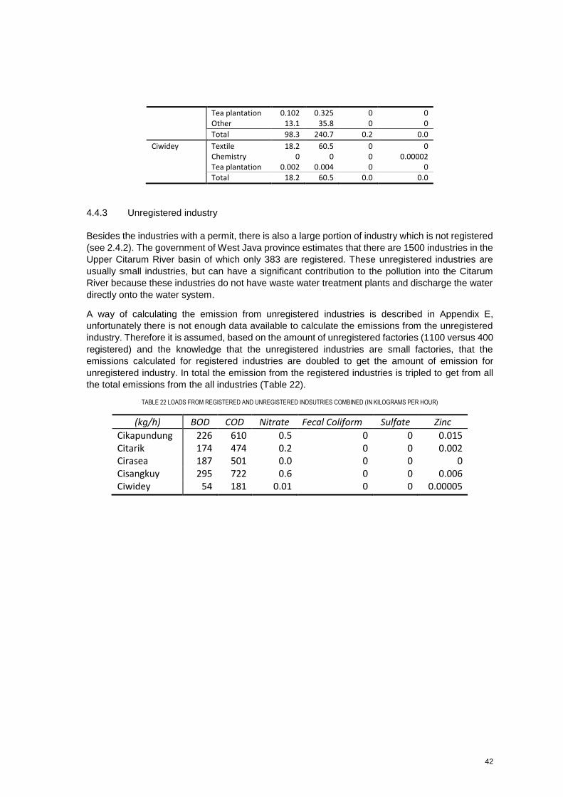
42
Tea plantation 0.102 0.325 0 0 Other 13.1 35.8 0 0
Total 98.3 240.7 0.2 0.0
Ciwidey Textile 18.2 60.5 0 0 Chemistry 0 0 0 0.00002 Tea plantation 0.002 0.004 0 0
Total 18.2 60.5 0.0 0.0
4.4.3 Unregistered industry
Besides the industries with a permit, there is also a large portion of industry which is not registered
(see 2.4.2). The government of West Java province estimates that there are 1500 industries in the
Upper Citarum River basin of which only 383 are registered. These unregistered industries are
usually small industries, but can have a significant contribution to the pollution into the Citarum
River because these industries do not have waste water treatment plants and discharge the water
directly onto the water system.
A way of calculating the emission from unregistered industries is described in Appendix E,
unfortunately there is not enough data available to calculate the emissions from the unregistered
industry. Therefore it is assumed, based on the amount of unregistered factories (1100 versus 400
registered) and the knowledge that the unregistered industries are small factories, that the
emissions calculated for registered industries are doubled to get the amount of emission for
unregistered industry. In total the emission from the registered industries is tripled to get from all
the total emissions from the all industries (Table 22).
TABLE 22 LOADS FROM REGISTERED AND UNREGISTERED INDSUTRIES COMBINED (IN KILOGRAMS PER HOUR)
(kg/h) BOD COD Nitrate Fecal Coliform Sulfate Zinc
Cikapundung 226 610 0.5 0 0 0.015 Citarik 174 474 0.2 0 0 0.002 Cirasea 187 501 0.0 0 0 0 Cisangkuy 295 722 0.6 0 0 0.006 Ciwidey 54 181 0.01 0 0 0.00005
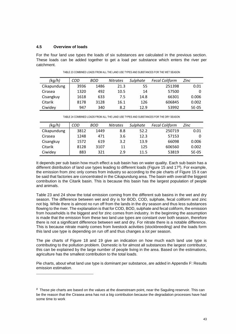
43
4.5 Overview of loads
For the four land use types the loads of six substances are calculated in the previous section.
These loads can be added together to get a load per substance which enters the river per
catchment.
TABLE 23 COMBINED LOADS FROM ALL THE LAND USE TYPES AND SUBSTANCES FOR THE WET SEASON
(kg/h) COD BOD Nitrates Sulphate Fecal Coliform Zinc
Cikapundung 3936 1486 21.3 55 251398 0.01 Cirasea 1320 492 10.5 14 57500 0 Cisangkuy 1618 633 7.5 14.8 66301 0.006 Citarik 8178 3128 16.1 126 606845 0.002 Ciwidey 947 340 8.2 12.9 53992 5E-05
TABLE 24 COMBINED LOADS FROM ALL THE LAND USE TYPES AND SUBSTANCES FOR THE DRY SEASON
(kg/h) COD BOD Nitrates Sulphate Fecal Coliform Zinc
Cikapundung 3812 1449 8.8 52.2 250719 0.01 Cirasea 1248 471 3.6 12.3 57153 0 Cisangkuy 1572 619 3.2 13.9 66098 0.006 Citarik 8128 3107 11 125 606560 0.002 Ciwidey 883 321 2.9 11.5 53819 5E-05
It depends per sub basin how much effect a sub basin has on water quality. Each sub basin has a different distribution of land use types leading to different loads (Figure 15 and 178). For example, the emission from zinc only comes from industry so according to the pie charts of Figure 15 it can be said that factories are concentrated in the Cikapundung area. The basin with overall the biggest contribution is the Citarik basin. This is because this basin has the largest population of people and animals. Table 23 and 24 show the total emission coming from the different sub basins in the wet and dry season. The difference between wet and dry is for BOD, COD, sulphate, fecal coliform and zinc not big. While there is almost no run off from the lands in the dry season and thus less substances flowing to the river. The explanation is that for COD, BOD, sulphate and fecal coliform, the emission from households is the biggest and for zinc comes from industry. In the beginning the assumption is made that the emission from these two land use types are constant over both season, therefore there is not a significant difference between wet and dry. For nitrate there is a notable difference. This is because nitrate mainly comes from livestock activities (stockbreeding) and the loads form this land use type is depending on run off and thus changes a lot per season. The pie charts of Figure 18 and 19 give an indication on how much each land use type is contributing to the pollution problem. Domestic is for almost all substances the largest contributor, this can be explained by the large number of people living in the area. Based on the estimations, agriculture has the smallest contribution to the total loads. Pie charts, about what land use type is dominant per substance, are added in Appendix F: Results emission estimation.
8 These pie charts are based on the values at the downstream point, near the Saguling reservoir. This can
be the reason that the Cirasea area has not a big contribution because the degradation processes have had
some time to work
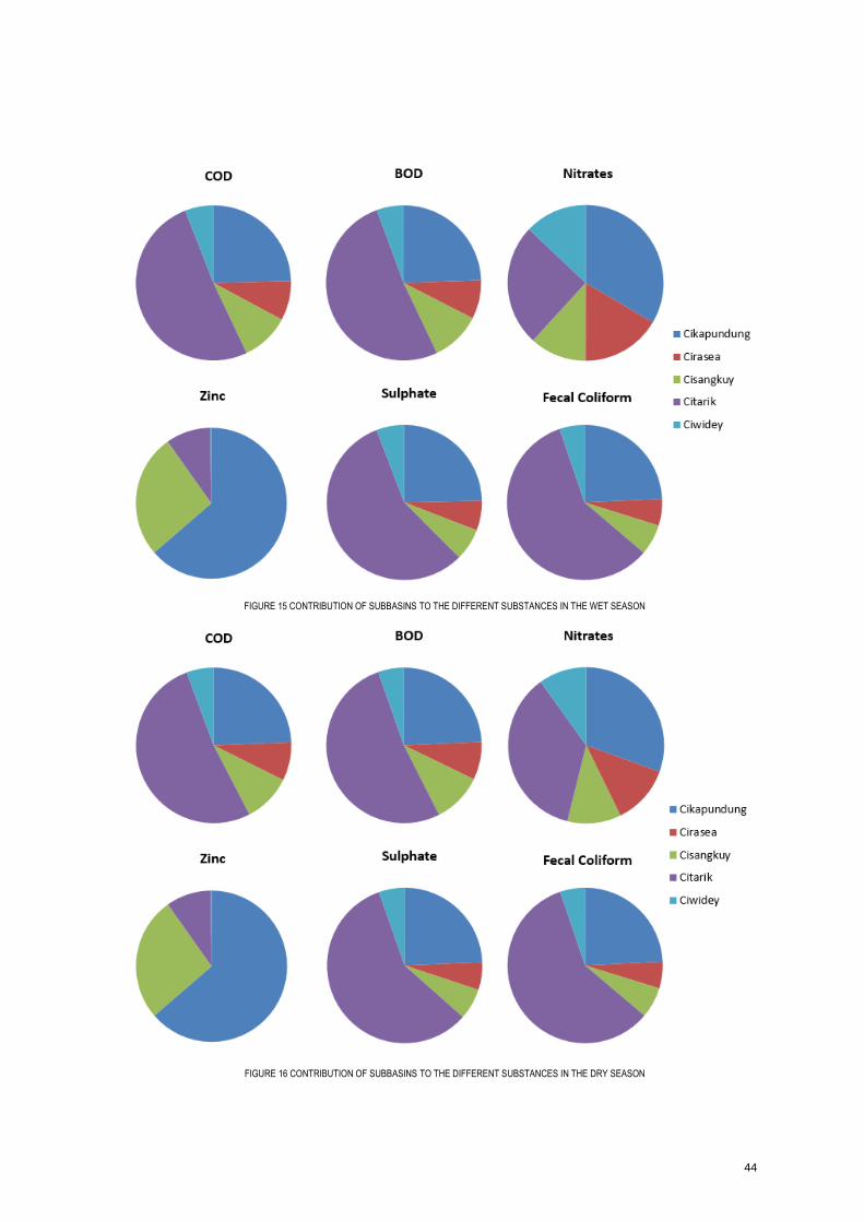
44
FIGURE 15 CONTRIBUTION OF SUBBASINS TO THE DIFFERENT SUBSTANCES IN THE WET SEASON
FIGURE 16 CONTRIBUTION OF SUBBASINS TO THE DIFFERENT SUBSTANCES IN THE DRY SEASON
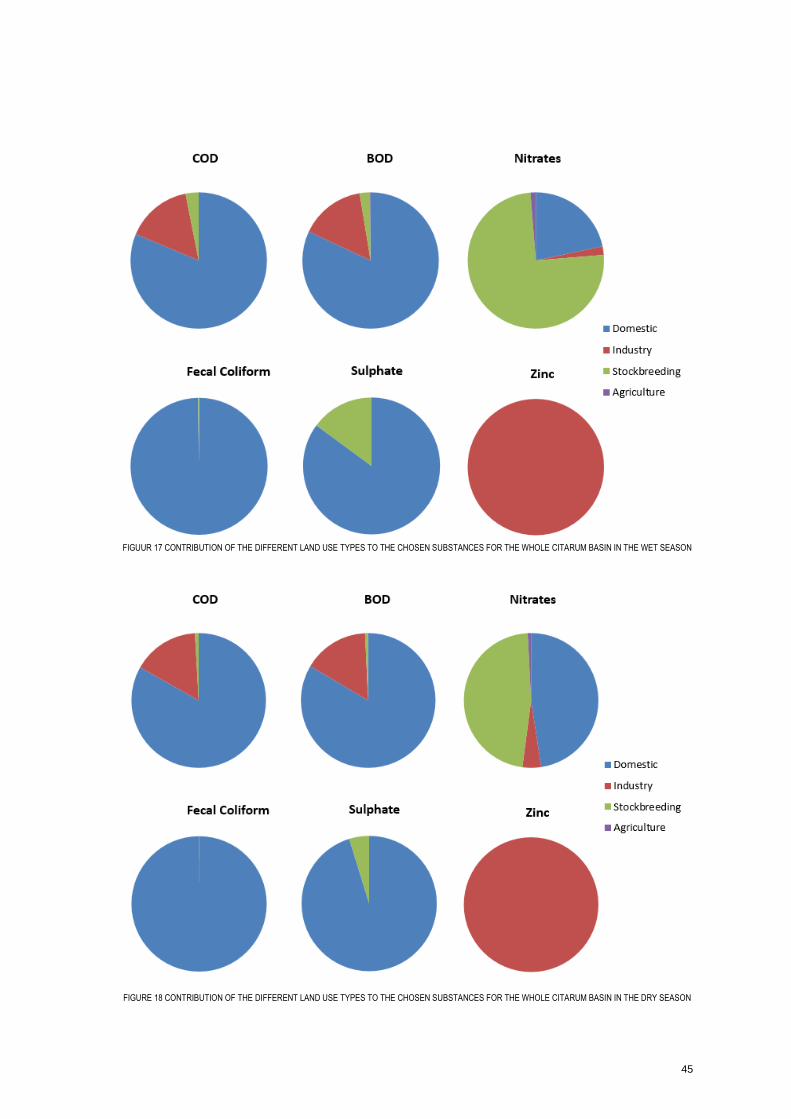
45
FIGUUR 17 CONTRIBUTION OF THE DIFFERENT LAND USE TYPES TO THE CHOSEN SUBSTANCES FOR THE WHOLE CITARUM BASIN IN THE WET SEASON
FIGURE 18 CONTRIBUTION OF THE DIFFERENT LAND USE TYPES TO THE CHOSEN SUBSTANCES FOR THE WHOLE CITARUM BASIN IN THE DRY SEASON
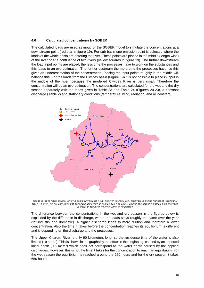
46
4.6 Calculated concentrations by SOBEK
The calculated loads are used as input for the SOBEK model to simulate the concentrations at a
downstream point (red star in figure 19). Per sub basin one emission point is selected where the
loads of the whole basin are entering the river. These points are placed in the middle (length wise)
of the river or at a confluence of two rivers (yellow squares in figure 19). The further downstream
the load input points are placed, the less time the processes have to work on the substances and
this leads to an overestimation. The further upstream the more time the processes have, so this
gives an underestimation of the concentration. Placing the input points roughly in the middle will
balance this. For the loads from the Ciwidey basin (Figure 19) it is not possible to place in input in
the middle of the river, because the modelled Ciwidey River is very small. Therefore the
concentration will be an overestimation. The concentrations are calculated for the wet and the dry
season separately with the loads given in Table 23 and Table 24 (Figures 20-23), a constant
discharge (Table 2) and stationary conditions (temperature, wind, radiation, and all constant).
FIGURE 19 UPPER CITARUM BASIN WITH THE RIVER SYSTEM AS IT IS IMPLEMENTED IN SOBEK, WITH BLUE TRIANGLES THE DISCHARGE INPUT FROM
TABLE 2, THE YELLOW SQUARES IS WIHERE THE LOADS ARE ADDED AS GIVEN IN TABLE 24 AND 25, AND THE RED STAR IS THE MEASURING POINT FOR
WHICH ALSO THE OUTPUT OF THE MODEL IS GENERATED
The difference between the concentrations in the wet and dry season in the figures below is
explained by the difference in discharge, where the loads stays roughly the same over the year
(for industry and domestic). A higher discharge leads to more dilution and therefore a lower
concentration. Also the time it takes before the concentration reaches its equilibrium is different
and is depending on the discharge and the processes.
The Upper Citarum River is only 90 kilometers long, so the residence time of the water is also
limited (19 hours). This is shown in the graphs by the offset in the beginning, caused by an imposed
initial depth (0.5 meter) which does not correspond to the water depth caused by the applied
discharges. However, this is not the time it takes for the concentration to reach an equilibrium. For
the wet season the equilibrium is reached around the 250 hours and for the dry season it takes
650 hours.
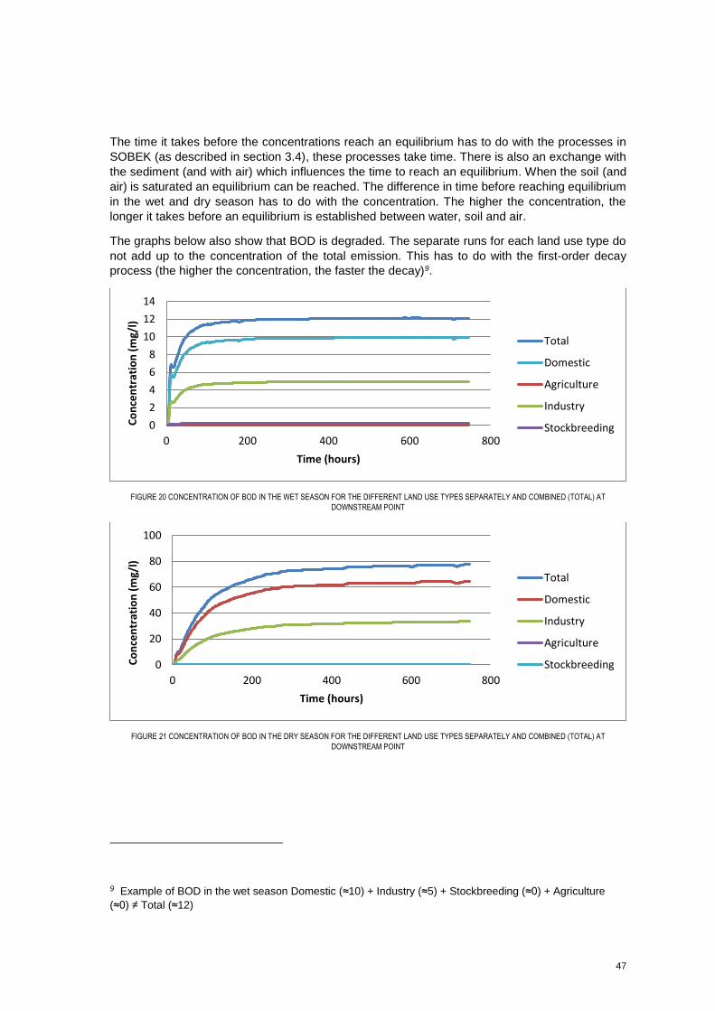
47
The time it takes before the concentrations reach an equilibrium has to do with the processes in
SOBEK (as described in section 3.4), these processes take time. There is also an exchange with
the sediment (and with air) which influences the time to reach an equilibrium. When the soil (and
air) is saturated an equilibrium can be reached. The difference in time before reaching equilibrium
in the wet and dry season has to do with the concentration. The higher the concentration, the
longer it takes before an equilibrium is established between water, soil and air.
The graphs below also show that BOD is degraded. The separate runs for each land use type do
not add up to the concentration of the total emission. This has to do with the first-order decay
process (the higher the concentration, the faster the decay)9.
FIGURE 20 CONCENTRATION OF BOD IN THE WET SEASON FOR THE DIFFERENT LAND USE TYPES SEPARATELY AND COMBINED (TOTAL) AT
DOWNSTREAM POINT
FIGURE 21 CONCENTRATION OF BOD IN THE DRY SEASON FOR THE DIFFERENT LAND USE TYPES SEPARATELY AND COMBINED (TOTAL) AT
DOWNSTREAM POINT
9 Example of BOD in the wet season Domestic (≈10) + Industry (≈5) + Stockbreeding (≈0) + Agriculture
(≈0) ≠ Total (≈12)
0
2
4
6
8
10
12
14
0 200 400 600 800
Co
nce
ntr
atio
n (
mg/
l)
Time (hours)
Total
Domestic
Agriculture
Industry
Stockbreeding
0
20
40
60
80
100
0 200 400 600 800
Co
nce
ntr
atio
n (
mg/
l)
Time (hours)
Total
Domestic
Industry
Agriculture
Stockbreeding
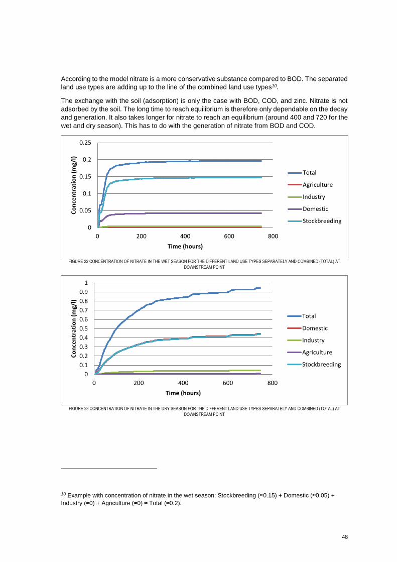
48
According to the model nitrate is a more conservative substance compared to BOD. The separated
land use types are adding up to the line of the combined land use types10.
The exchange with the soil (adsorption) is only the case with BOD, COD, and zinc. Nitrate is not
adsorbed by the soil. The long time to reach equilibrium is therefore only dependable on the decay
and generation. It also takes longer for nitrate to reach an equilibrium (around 400 and 720 for the
wet and dry season). This has to do with the generation of nitrate from BOD and COD.
FIGURE 22 CONCENTRATION OF NITRATE IN THE WET SEASON FOR THE DIFFERENT LAND USE TYPES SEPARATELY AND COMBINED (TOTAL) AT
DOWNSTREAM POINT
FIGURE 23 CONCENTRATION OF NITRATE IN THE DRY SEASON FOR THE DIFFERENT LAND USE TYPES SEPARATELY AND COMBINED (TOTAL) AT
DOWNSTREAM POINT
10 Example with concentration of nitrate in the wet season: Stockbreeding (≈0.15) + Domestic (≈0.05) +
Industry (≈0) + Agriculture (≈0) ≈ Total (≈0.2).
0
0.05
0.1
0.15
0.2
0.25
0 200 400 600 800
Co
nce
ntr
atio
n (
mg/
l)
Time (hours)
Total
Agriculture
Industry
Domestic
Stockbreeding
0
0.1
0.2
0.3
0.4
0.5
0.6
0.7
0.8
0.9
1
0 200 400 600 800
Co
nce
ntr
atio
n (
mg/
l)
Time (hours)
Total
Domestic
Industry
Agriculture
Stockbreeding
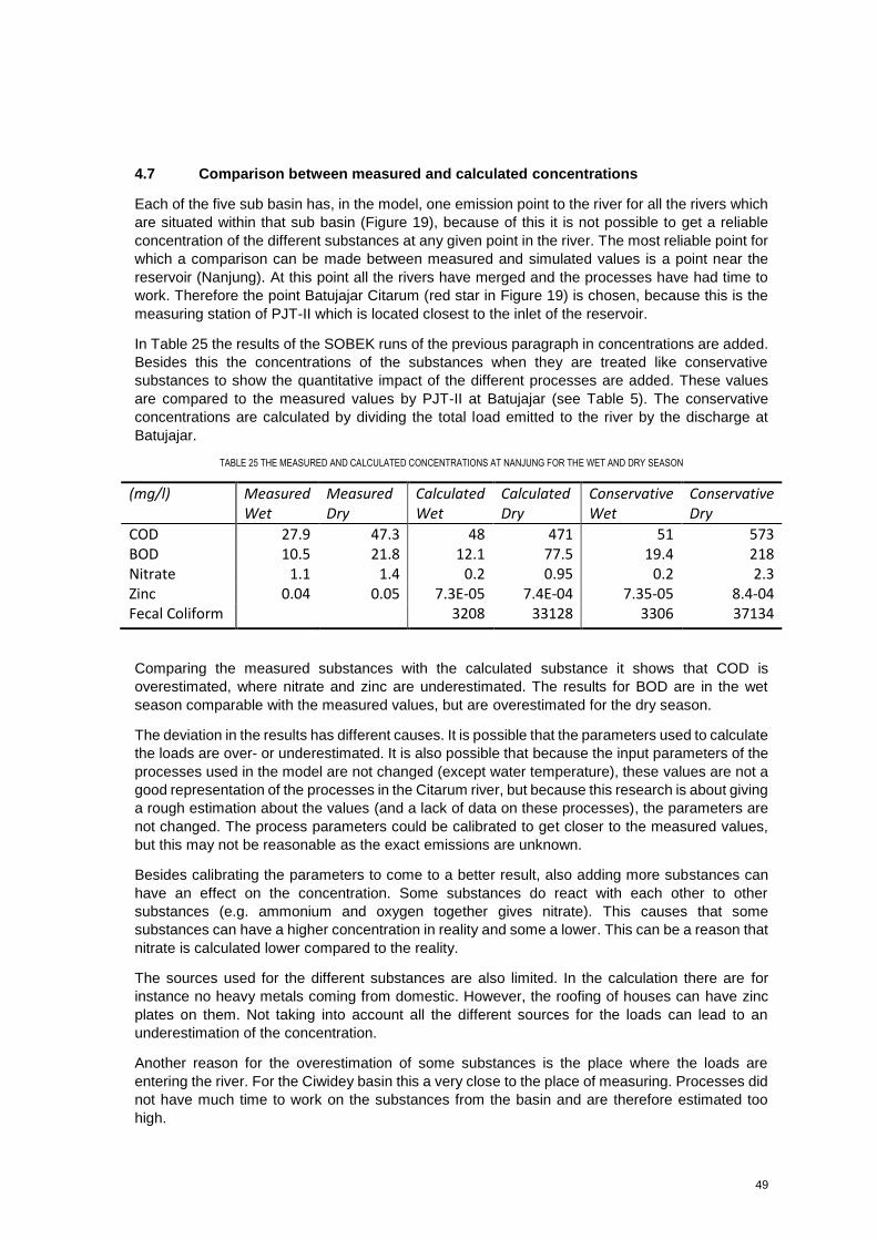
49
4.7 Comparison between measured and calculated concentrations Each of the five sub basin has, in the model, one emission point to the river for all the rivers which
are situated within that sub basin (Figure 19), because of this it is not possible to get a reliable
concentration of the different substances at any given point in the river. The most reliable point for
which a comparison can be made between measured and simulated values is a point near the
reservoir (Nanjung). At this point all the rivers have merged and the processes have had time to
work. Therefore the point Batujajar Citarum (red star in Figure 19) is chosen, because this is the
measuring station of PJT-II which is located closest to the inlet of the reservoir.
In Table 25 the results of the SOBEK runs of the previous paragraph in concentrations are added.
Besides this the concentrations of the substances when they are treated like conservative
substances to show the quantitative impact of the different processes are added. These values
are compared to the measured values by PJT-II at Batujajar (see Table 5). The conservative
concentrations are calculated by dividing the total load emitted to the river by the discharge at
Batujajar.
TABLE 25 THE MEASURED AND CALCULATED CONCENTRATIONS AT NANJUNG FOR THE WET AND DRY SEASON
(mg/l) Measured Wet
Measured Dry
Calculated Wet
Calculated Dry
Conservative Wet
Conservative Dry
COD 27.9 47.3 48 471 51 573 BOD 10.5 21.8 12.1 77.5 19.4 218 Nitrate 1.1 1.4 0.2 0.95 0.2 2.3 Zinc 0.04 0.05 7.3E-05 7.4E-04 7.35-05 8.4-04 Fecal Coliform 3208 33128 3306 37134
Comparing the measured substances with the calculated substance it shows that COD is
overestimated, where nitrate and zinc are underestimated. The results for BOD are in the wet
season comparable with the measured values, but are overestimated for the dry season.
The deviation in the results has different causes. It is possible that the parameters used to calculate
the loads are over- or underestimated. It is also possible that because the input parameters of the
processes used in the model are not changed (except water temperature), these values are not a
good representation of the processes in the Citarum river, but because this research is about giving
a rough estimation about the values (and a lack of data on these processes), the parameters are
not changed. The process parameters could be calibrated to get closer to the measured values,
but this may not be reasonable as the exact emissions are unknown.
Besides calibrating the parameters to come to a better result, also adding more substances can
have an effect on the concentration. Some substances do react with each other to other
substances (e.g. ammonium and oxygen together gives nitrate). This causes that some
substances can have a higher concentration in reality and some a lower. This can be a reason that
nitrate is calculated lower compared to the reality.
The sources used for the different substances are also limited. In the calculation there are for
instance no heavy metals coming from domestic. However, the roofing of houses can have zinc
plates on them. Not taking into account all the different sources for the loads can lead to an
underestimation of the concentration.
Another reason for the overestimation of some substances is the place where the loads are
entering the river. For the Ciwidey basin this a very close to the place of measuring. Processes did
not have much time to work on the substances from the basin and are therefore estimated too
high.
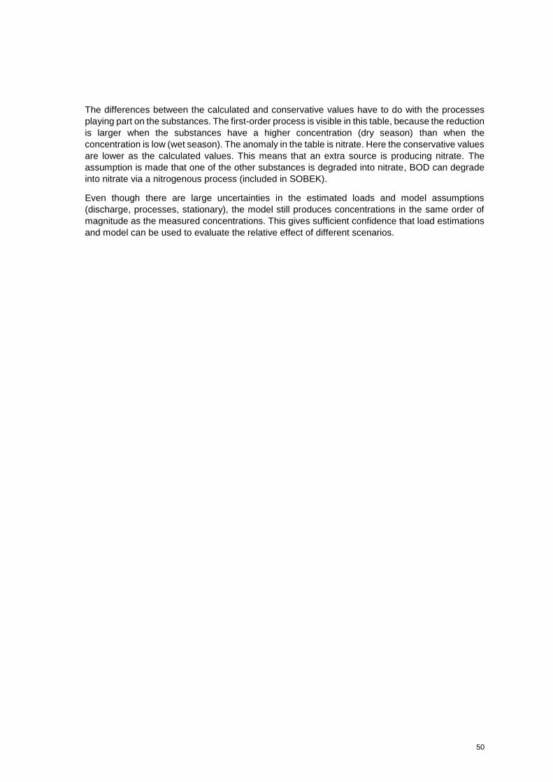
50
The differences between the calculated and conservative values have to do with the processes
playing part on the substances. The first-order process is visible in this table, because the reduction
is larger when the substances have a higher concentration (dry season) than when the
concentration is low (wet season). The anomaly in the table is nitrate. Here the conservative values
are lower as the calculated values. This means that an extra source is producing nitrate. The
assumption is made that one of the other substances is degraded into nitrate, BOD can degrade
into nitrate via a nitrogenous process (included in SOBEK).
Even though there are large uncertainties in the estimated loads and model assumptions
(discharge, processes, stationary), the model still produces concentrations in the same order of
magnitude as the measured concentrations. This gives sufficient confidence that load estimations
and model can be used to evaluate the relative effect of different scenarios.
51
5 SCENARIOS
The interviews with the stakeholders are used to define scenarios. To give the stakeholders more
insight in were to start to improve the impaired water quality is key in this research. The solutions
which are named the most by the stakeholders for the improvement of the water quality are put
into scenarios. With the quantification of the emissions in previous chapter it is possible to estimate
the changes in these emissions due to the different scenarios. This chapter gives the scenarios
and the subsequent changes to the emission data.
The next scenarios are chosen to model:
Reference scenario The current status in 2015 is used as reference scenario
Worst case scenario 2030 An autonomous growth of population and economy is combined
with the current status of policies to come to a worst case
scenario
Improved sanitation The people without any sanitation facilities are given a septic
tank
Livestock in communal barns The dispersed cattle is concentrated on a few places in barns
to control the emission
Changing crops The paddy fields are changed into fields for dry crops
Changing industry This are three scenarios in one. First all the industries are
deleted from the system, secondly only the textile industry is
deleted, and third the textile factories are converted to other
types of industry
5.1 Reference scenario
This scenario is the current situation of the river. This situation is represented by the simulations
of Chapter 4. The calculated concentration (Table 25) will be used as a reference to assess the
effect of the different scenarios on water quality.
5.2 Worst case scenario 2030
When the authorities do nothing to improve the water quality, but the population and economy
keeps on growing, this scenario can become reality.
The trend for population growth is an increase of 50 million in Indonesia in the next 15 years. This
is an increase of 20 percent (Figure 24). This leads to an increase of domestic waste of also 20
percent. The assumption is made that the people are spreading evenly throughout the basin so
every area gets 20 percent more people.
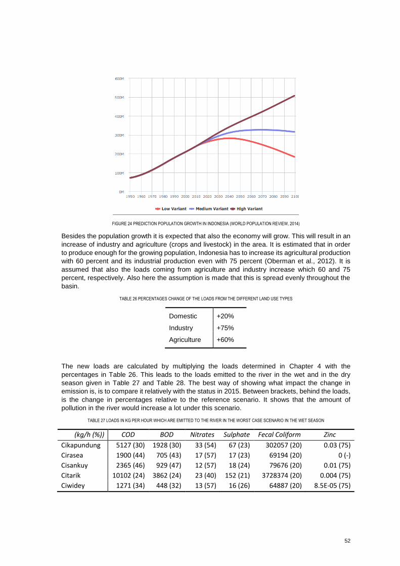
52
FIGURE 24 PREDICTION POPULATION GROWTH IN INDONESIA (WORLD POPULATION REVIEW, 2014)
Besides the population growth it is expected that also the economy will grow. This will result in an
increase of industry and agriculture (crops and livestock) in the area. It is estimated that in order
to produce enough for the growing population, Indonesia has to increase its agricultural production
with 60 percent and its industrial production even with 75 percent (Oberman et al., 2012). It is
assumed that also the loads coming from agriculture and industry increase which 60 and 75
percent, respectively. Also here the assumption is made that this is spread evenly throughout the
basin.
TABLE 26 PERCENTAGES CHANGE OF THE LOADS FROM THE DIFFERENT LAND USE TYPES
Domestic +20%
Industry +75%
Agriculture +60%
The new loads are calculated by multiplying the loads determined in Chapter 4 with the
percentages in Table 26. This leads to the loads emitted to the river in the wet and in the dry
season given in Table 27 and Table 28. The best way of showing what impact the change in
emission is, is to compare it relatively with the status in 2015. Between brackets, behind the loads,
is the change in percentages relative to the reference scenario. It shows that the amount of
pollution in the river would increase a lot under this scenario.
TABLE 27 LOADS IN KG PER HOUR WHICH ARE EMITTED TO THE RIVER IN THE WORST CASE SCENARIO IN THE WET SEASON
(kg/h (%)) COD BOD Nitrates Sulphate Fecal Coliform Zinc
Cikapundung 5127 (30) 1928 (30) 33 (54) 67 (23) 302057 (20) 0.03 (75)
Cirasea 1900 (44) 705 (43) 17 (57) 17 (23) 69194 (20) 0 (-)
Cisankuy 2365 (46) 929 (47) 12 (57) 18 (24) 79676 (20) 0.01 (75)
Citarik 10102 (24) 3862 (24) 23 (40) 152 (21) 3728374 (20) 0.004 (75)
Ciwidey 1271 (34) 448 (32) 13 (57) 16 (26) 64887 (20) 8.5E-05 (75)
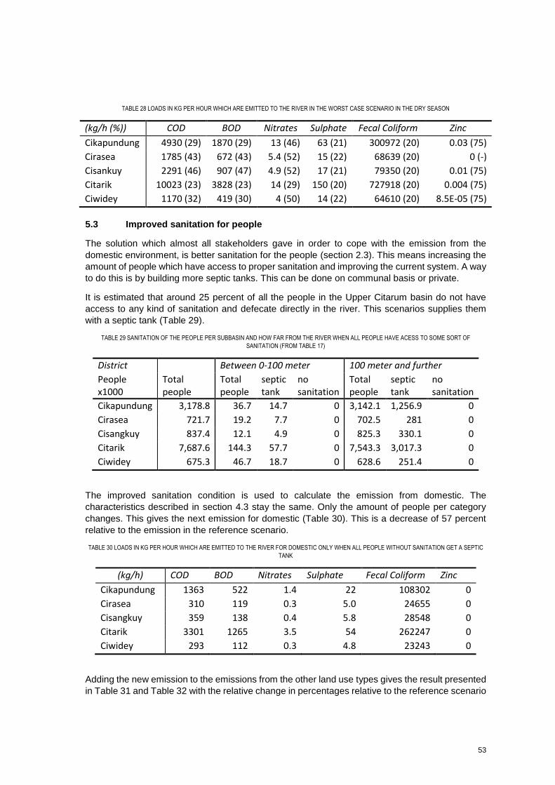
53
TABLE 28 LOADS IN KG PER HOUR WHICH ARE EMITTED TO THE RIVER IN THE WORST CASE SCENARIO IN THE DRY SEASON
(kg/h (%)) COD BOD Nitrates Sulphate Fecal Coliform Zinc
Cikapundung 4930 (29) 1870 (29) 13 (46) 63 (21) 300972 (20) 0.03 (75)
Cirasea 1785 (43) 672 (43) 5.4 (52) 15 (22) 68639 (20) 0 (-)
Cisankuy 2291 (46) 907 (47) 4.9 (52) 17 (21) 79350 (20) 0.01 (75)
Citarik 10023 (23) 3828 (23) 14 (29) 150 (20) 727918 (20) 0.004 (75)
Ciwidey 1170 (32) 419 (30) 4 (50) 14 (22) 64610 (20) 8.5E-05 (75)
5.3 Improved sanitation for people
The solution which almost all stakeholders gave in order to cope with the emission from the
domestic environment, is better sanitation for the people (section 2.3). This means increasing the
amount of people which have access to proper sanitation and improving the current system. A way
to do this is by building more septic tanks. This can be done on communal basis or private.
It is estimated that around 25 percent of all the people in the Upper Citarum basin do not have
access to any kind of sanitation and defecate directly in the river. This scenarios supplies them
with a septic tank (Table 29).
TABLE 29 SANITATION OF THE PEOPLE PER SUBBASIN AND HOW FAR FROM THE RIVER WHEN ALL PEOPLE HAVE ACESS TO SOME SORT OF
SANITATION (FROM TABLE 17)
District Between 0-100 meter 100 meter and further
People x1000
Total people
Total people
septic tank
no sanitation
Total people
septic tank
no sanitation
Cikapundung 3,178.8 36.7 14.7 0 3,142.1 1,256.9 0
Cirasea 721.7 19.2 7.7 0 702.5 281 0
Cisangkuy 837.4 12.1 4.9 0 825.3 330.1 0
Citarik 7,687.6 144.3 57.7 0 7,543.3 3,017.3 0
Ciwidey 675.3 46.7 18.7 0 628.6 251.4 0
The improved sanitation condition is used to calculate the emission from domestic. The
characteristics described in section 4.3 stay the same. Only the amount of people per category
changes. This gives the next emission for domestic (Table 30). This is a decrease of 57 percent
relative to the emission in the reference scenario.
TABLE 30 LOADS IN KG PER HOUR WHICH ARE EMITTED TO THE RIVER FOR DOMESTIC ONLY WHEN ALL PEOPLE WITHOUT SANITATION GET A SEPTIC
TANK
(kg/h) COD BOD Nitrates Sulphate Fecal Coliform Zinc
Cikapundung 1363 522 1.4 22 108302 0
Cirasea 310 119 0.3 5.0 24655 0
Cisangkuy 359 138 0.4 5.8 28548 0
Citarik 3301 1265 3.5 54 262247 0
Ciwidey 293 112 0.3 4.8 23243 0
Adding the new emission to the emissions from the other land use types gives the result presented
in Table 31 and Table 32 with the relative change in percentages relative to the reference scenario
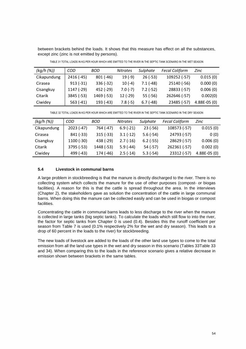
54
between brackets behind the loads. It shows that this measure has effect on all the substances,
except zinc (zinc is not emitted by persons).
TABLE 31 TOTAL LOADS IN KG PER HOUR WHICH ARE EMITTED TO THE RIVER IN THE SEPTIC TANK SCENARIO IN THE WET SEASON
(kg/h (%)) COD BOD Nitrates Sulphate Fecal Coliform Zinc
Cikapundung 2416 (-45) 801 (-46) 19 (-9) 26 (-53) 109252 (-57) 0.015 (0)
Cirasea 913 (-31) 336 (-32) 10 (-4) 7.1 (-48) 25140 (-56) 0.000 (0)
Cisangkuy 1147 (-29) 452 (-29) 7.0 (-7) 7.2 (-52) 28833 (-57) 0.006 (0)
Citarik 3845 (-53) 1469 (-53) 12 (-29) 55 (-56) 262646 (-57) 0.002(0)
Ciwidey 563 (-41) 193 (-43) 7.8 (-5) 6.7 (-48) 23485 (-57) 4.88E-05 (0)
TABLE 32 TOTAL LOADS IN KG PER HOUR WHICH ARE EMITTED TO THE RIVER IN THE SEPTIC TANK SCENARIO IN THE DRY SEASON
(kg/h (%)) COD BOD Nitrates Sulphate Fecal Coliform Zinc
Cikapundung 2023 (-47) 764 (-47) 6.9 (-21) 23 (-56) 108573 (-57) 0.015 (0)
Cirasea 841 (-33) 315 (-33) 3.1 (-12) 5.6 (-54) 24793 (-57) 0 (0)
Cisangkuy 1100 (-30) 438 (-29) 2.7 (-16) 6.2 (-55) 28629 (-57) 0.006 (0)
Citarik 3795 (-53) 1448 (-53) 5.9 (-44) 54 (-57) 262361 (-57) 0.002 (0)
Ciwidey 499 (-43) 174 (-46) 2.5 (-14) 5.3 (-54) 23312 (-57) 4.88E-05 (0)
5.4 Livestock in communal barns
A large problem in stockbreeding is that the manure is directly discharged to the river. There is no
collecting system which collects the manure for the use of other purposes (compost- or biogas
facilities). A reason for this is that the cattle is spread throughout the area. In the interviews
(Chapter 2), the stakeholders gave as solution the concentration of the cattle in large communal
barns. When doing this the manure can be collected easily and can be used in biogas or compost
facilities.
Concentrating the cattle in communal barns leads to less discharge to the river when the manure is collected in large tanks (big septic tanks). To calculate the loads which still flow to into the river, the factor for septic tanks from Chapter 0 is used (0.4). Besides this the runoff coefficient per season from Table 7 is used (0.1% respectively 2% for the wet and dry season). This leads to a drop of 60 percent in the loads to the river) for stockbreeding. The new loads of livestock are added to the loads of the other land use types to come to the total
emission from all the land use types in the wet and dry season in this scenario (Tables 33Table 33
and 34). When comparing this to the loads in the reference scenario gives a relative decrease in
emission shown between brackets in the same tables.
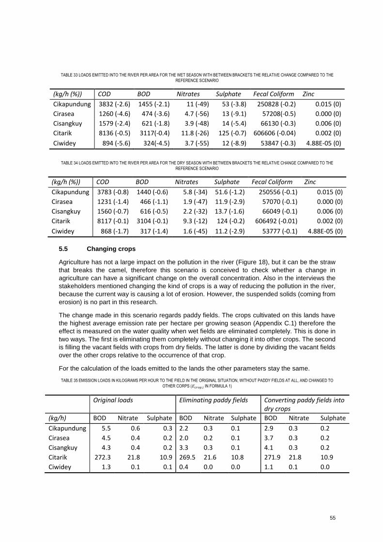
55
TABLE 33 LOADS EMITTED INTO THE RIVER PER AREA FOR THE WET SEASON WITH BETWEEN BRACKETS THE RELATIVE CHANGE COMPARED TO THE
REFERENCE SCENARIO
(kg/h (%)) COD BOD Nitrates Sulphate Fecal Coliform Zinc
Cikapundung 3832 (-2.6) 1455 (-2.1) 11 (-49) 53 (-3.8) 250828 (-0.2) 0.015 (0)
Cirasea 1260 (-4.6) 474 (-3.6) 4.7 (-56) 13 (-9.1) 57208(-0.5) 0.000 (0)
Cisangkuy 1579 (-2.4) 621 (-1.8) 3.9 (-48) 14 (-5.4) 66130 (-0.3) 0.006 (0)
Citarik 8136 (-0.5) 3117(-0.4) 11.8 (-26) 125 (-0.7) 606606 (-0.04) 0.002 (0)
Ciwidey 894 (-5.6) 324(-4.5) 3.7 (-55) 12 (-8.9) 53847 (-0.3) 4.88E-05 (0)
TABLE 34 LOADS EMITTED INTO THE RIVER PER AREA FOR THE DRY SEASON WITH BETWEEN BRACKETS THE RELATIVE CHANGE COMPARED TO THE
REFERENCE SCENARIO
(kg/h (%)) COD BOD Nitrates Sulphate Fecal Coliform Zinc
Cikapundung 3783 (-0.8) 1440 (-0.6) 5.8 (-34) 51.6 (-1.2) 250556 (-0.1) 0.015 (0)
Cirasea 1231 (-1.4) 466 (-1.1) 1.9 (-47) 11.9 (-2.9) 57070 (-0.1) 0.000 (0)
Cisangkuy 1560 (-0.7) 616 (-0.5) 2.2 (-32) 13.7 (-1.6) 66049 (-0.1) 0.006 (0)
Citarik 8117 (-0.1) 3104 (-0.1) 9.3 (-12) 124 (-0.2) 606492 (-0.01) 0.002 (0)
Ciwidey 868 (-1.7) 317 (-1.4) 1.6 (-45) 11.2 (-2.9) 53777 (-0.1) 4.88E-05 (0)
5.5 Changing crops
Agriculture has not a large impact on the pollution in the river (Figure 18), but it can be the straw
that breaks the camel, therefore this scenario is conceived to check whether a change in
agriculture can have a significant change on the overall concentration. Also in the interviews the
stakeholders mentioned changing the kind of crops is a way of reducing the pollution in the river,
because the current way is causing a lot of erosion. However, the suspended solids (coming from
erosion) is no part in this research.
The change made in this scenario regards paddy fields. The crops cultivated on this lands have
the highest average emission rate per hectare per growing season (Appendix C.1) therefore the
effect is measured on the water quality when wet fields are eliminated completely. This is done in
two ways. The first is eliminating them completely without changing it into other crops. The second
is filling the vacant fields with crops from dry fields. The latter is done by dividing the vacant fields
over the other crops relative to the occurrence of that crop.
For the calculation of the loads emitted to the lands the other parameters stay the same.
TABLE 35 EMISSION LOADS IN KILOGRAMS PER HOUR TO THE FIELD IN THE ORIGINAL SITUATION, WITHOUT PADDY FIELDS AT ALL, AND CHANGED TO
OTHER CORPS (𝐸𝑐𝑟𝑜𝑝,𝑖 IN FORMULA 1)
Original loads Eliminating paddy fields Converting paddy fields into dry crops
(kg/h) BOD Nitrate Sulphate BOD Nitrate Sulphate BOD Nitrate Sulphate
Cikapundung 5.5 0.6 0.3 2.2 0.3 0.1 2.9 0.3 0.2
Cirasea 4.5 0.4 0.2 2.0 0.2 0.1 3.7 0.3 0.2
Cisangkuy 4.3 0.4 0.2 3.3 0.3 0.1 4.1 0.3 0.2
Citarik 272.3 21.8 10.9 269.5 21.6 10.8 271.9 21.8 10.9
Ciwidey 1.3 0.1 0.1 0.4 0.0 0.0 1.1 0.1 0.0
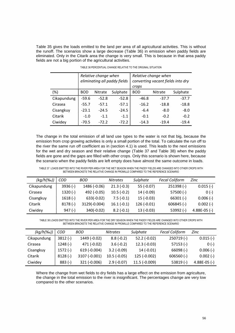
56
Table 35 gives the loads emitted to the land per area of all agricultural activities. This is without the runoff. The scenarios show a large decrease (Table 36) in emission when paddy fields are eliminated. Only in the Citarik area the change is very small. This is because in that area paddy fields are not a big portion of the agricultural activities.
TABLE 36 PERCENTUAL CHANGE RELATIVE TO THE ORIGINAL SITUATION
Relative change when eliminating all paddy fields
Relative change when converting vacant fields into dry crops
(%) BOD Nitrate Sulphate BOD Nitrate Sulphate
Cikapundung -59.6 -52.8 -52.8 -46.8 -37.7 -37.7
Cirasea -55.7 -57.1 -57.1 -16.2 -18.8 -18.8
Cisangkuy -23.1 -24.5 -24.5 -6.4 -8.0 -8.0
Citarik -1.0 -1.1 -1.1 -0.1 -0.2 -0.2
Ciwidey -70.5 -72.2 -72.2 -14.3 -19.4 -19.4
The change in the total emission of all land use types to the water is not that big, because the
emission from crop growing activities is only a small portion of the total. To calculate the run off to
the river the same run off coefficient as in (section 4.1) is used. This leads to the next emissions
for the wet and dry season and their relative change (Table 37 and Table 38) when the paddy
fields are gone and the gaps are filled with other crops. Only this scenario is shown here, because
the scenario when the paddy fields are left empty does have almost the same outcome in loads.
TABLE 37 LOADS EMITTED INTO THE RIVER PER AREA FOR THE WET SEASON WHEN THE PADDY FIELDS ARE CHANGED INTO OTHER CROPS WITH
BETWEEN BRACKETS THE RELATIVE CHANGE IN PROMILLE COMPARED TO THE REFERENCE SCENARIO
(kg/h(‰)) COD BOD Nitrates Sulphate Fecal Coliform Zinc
Cikapundung 3936 (-) 1486 (-0.06) 21.3 (-0.3) 55 (-0.07) 251398 (-) 0.015 (-)
Cirasea 1320 (-) 492 (-0.05) 10.5 (-0.2) 14 (-0.09) 57500 (-) 0 (-)
Cisangkuy 1618 (-) 633(-0.02) 7.5 (-0.1) 15 (-0.03) 66301 (-) 0.006 (-)
Citarik 8178 (-) 3129(-0.004) 16.1 (-0.1) 126 (-0.01) 606845 (-) 0.002 (-)
Ciwidey 947 (-) 340(-0.02) 8.2 (-0.1) 13 (-0.03) 53992 (-) 4.88E-05 (-)
TABLE 38 LOADS EMITTED INTO THE RIVER PER AREA FOR THE DRY SEASON WHEN THE PADDY FIELDS ARE CHANGED INTO OTHER CROPS WITH
BETWEEN BRACKETS THE RELATIVE CHANGE IN PROMILLE COMPARED TO THE REFERENCE SCENARIO
(kg/h(‰)) COD BOD Nitrates Sulphate Fecal Coliform Zinc
Cikapundung 3812 (-) 1449 (-0.02) 8.8 (-0.2) 52.2 (-0.02) 250719 (-) 0.015 (-)
Cirasea 1248 (-) 471 (-0.02) 3.6 (-0.2) 12.3 (-0.03) 57153 (-) 0 (-)
Cisangkuy 1572 (-) 619 (-0.004) 3.2 (-0.09) 14 (-0.01) 66098 (-) 0.006 (-)
Citarik 8128 (-) 3107 (-0.001) 10.5 (-0.05) 125 (-0.002) 606560 (-) 0.002 (-)
Ciwidey 883 (-) 321 (-0.006) 2.9 (-0.07) 11.5 (-0.009) 53819 (-) 4.88E-05 (-)
Where the change from wet fields to dry fields has a large effect on the emission from agriculture, the change in the total emission to the river is insignificant. The percentages change are very low compared to the other scenarios.
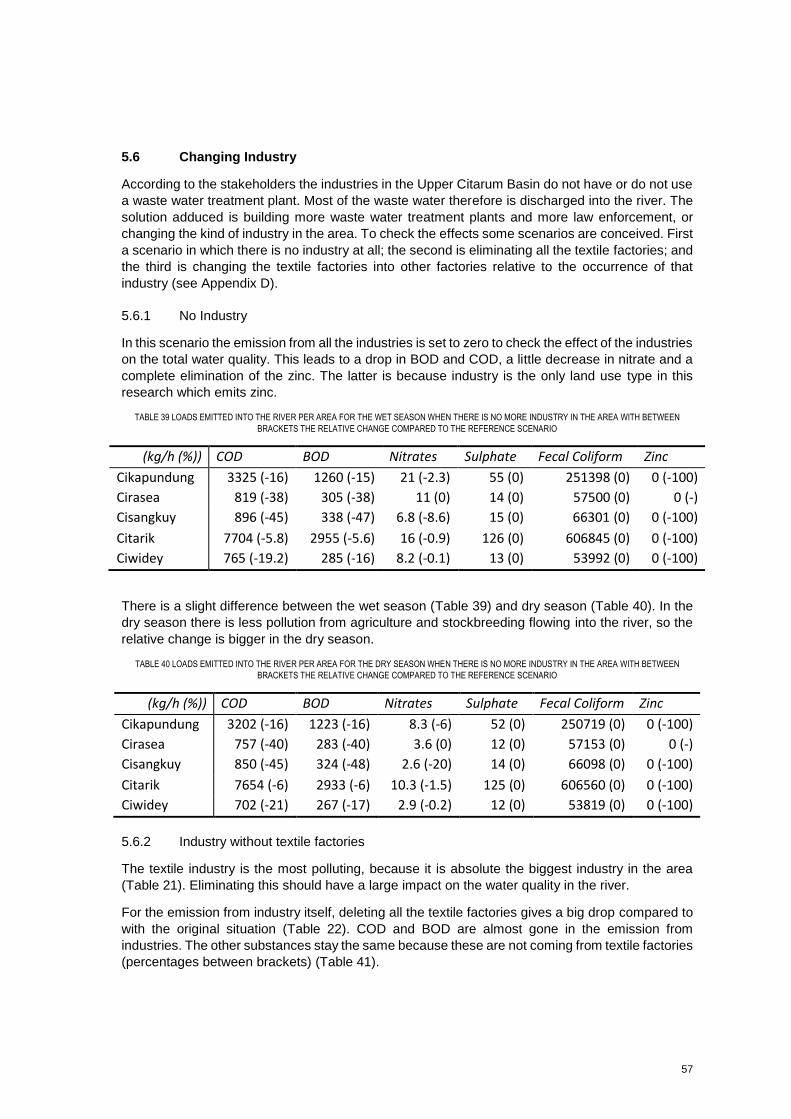
57
5.6 Changing Industry
According to the stakeholders the industries in the Upper Citarum Basin do not have or do not use
a waste water treatment plant. Most of the waste water therefore is discharged into the river. The
solution adduced is building more waste water treatment plants and more law enforcement, or
changing the kind of industry in the area. To check the effects some scenarios are conceived. First
a scenario in which there is no industry at all; the second is eliminating all the textile factories; and
the third is changing the textile factories into other factories relative to the occurrence of that
industry (see Appendix D).
5.6.1 No Industry
In this scenario the emission from all the industries is set to zero to check the effect of the industries
on the total water quality. This leads to a drop in BOD and COD, a little decrease in nitrate and a
complete elimination of the zinc. The latter is because industry is the only land use type in this
research which emits zinc.
TABLE 39 LOADS EMITTED INTO THE RIVER PER AREA FOR THE WET SEASON WHEN THERE IS NO MORE INDUSTRY IN THE AREA WITH BETWEEN
BRACKETS THE RELATIVE CHANGE COMPARED TO THE REFERENCE SCENARIO
(kg/h (%)) COD BOD Nitrates Sulphate Fecal Coliform Zinc
Cikapundung 3325 (-16) 1260 (-15) 21 (-2.3) 55 (0) 251398 (0) 0 (-100)
Cirasea 819 (-38) 305 (-38) 11 (0) 14 (0) 57500 (0) 0 (-)
Cisangkuy 896 (-45) 338 (-47) 6.8 (-8.6) 15 (0) 66301 (0) 0 (-100)
Citarik 7704 (-5.8) 2955 (-5.6) 16 (-0.9) 126 (0) 606845 (0) 0 (-100)
Ciwidey 765 (-19.2) 285 (-16) 8.2 (-0.1) 13 (0) 53992 (0) 0 (-100)
There is a slight difference between the wet season (Table 39) and dry season (Table 40). In the
dry season there is less pollution from agriculture and stockbreeding flowing into the river, so the
relative change is bigger in the dry season.
TABLE 40 LOADS EMITTED INTO THE RIVER PER AREA FOR THE DRY SEASON WHEN THERE IS NO MORE INDUSTRY IN THE AREA WITH BETWEEN
BRACKETS THE RELATIVE CHANGE COMPARED TO THE REFERENCE SCENARIO
(kg/h (%)) COD BOD Nitrates Sulphate Fecal Coliform Zinc
Cikapundung 3202 (-16) 1223 (-16) 8.3 (-6) 52 (0) 250719 (0) 0 (-100)
Cirasea 757 (-40) 283 (-40) 3.6 (0) 12 (0) 57153 (0) 0 (-)
Cisangkuy 850 (-45) 324 (-48) 2.6 (-20) 14 (0) 66098 (0) 0 (-100)
Citarik 7654 (-6) 2933 (-6) 10.3 (-1.5) 125 (0) 606560 (0) 0 (-100)
Ciwidey 702 (-21) 267 (-17) 2.9 (-0.2) 12 (0) 53819 (0) 0 (-100)
5.6.2 Industry without textile factories
The textile industry is the most polluting, because it is absolute the biggest industry in the area
(Table 21). Eliminating this should have a large impact on the water quality in the river.
For the emission from industry itself, deleting all the textile factories gives a big drop compared to
with the original situation (Table 22). COD and BOD are almost gone in the emission from
industries. The other substances stay the same because these are not coming from textile factories
(percentages between brackets) (Table 41).
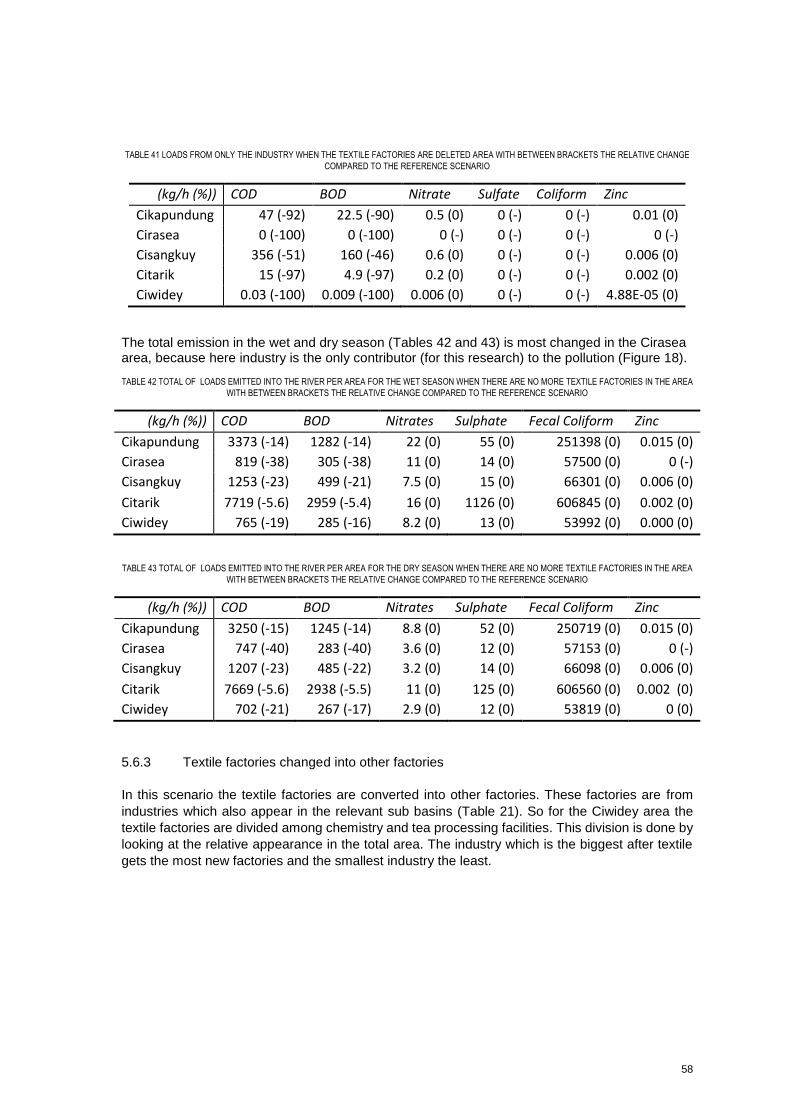
58
TABLE 41 LOADS FROM ONLY THE INDUSTRY WHEN THE TEXTILE FACTORIES ARE DELETED AREA WITH BETWEEN BRACKETS THE RELATIVE CHANGE
COMPARED TO THE REFERENCE SCENARIO
(kg/h (%)) COD BOD Nitrate Sulfate Coliform Zinc
Cikapundung 47 (-92) 22.5 (-90) 0.5 (0) 0 (-) 0 (-) 0.01 (0)
Cirasea 0 (-100) 0 (-100) 0 (-) 0 (-) 0 (-) 0 (-)
Cisangkuy 356 (-51) 160 (-46) 0.6 (0) 0 (-) 0 (-) 0.006 (0)
Citarik 15 (-97) 4.9 (-97) 0.2 (0) 0 (-) 0 (-) 0.002 (0)
Ciwidey 0.03 (-100) 0.009 (-100) 0.006 (0) 0 (-) 0 (-) 4.88E-05 (0)
The total emission in the wet and dry season (Tables 42 and 43) is most changed in the Cirasea area, because here industry is the only contributor (for this research) to the pollution (Figure 18). TABLE 42 TOTAL OF LOADS EMITTED INTO THE RIVER PER AREA FOR THE WET SEASON WHEN THERE ARE NO MORE TEXTILE FACTORIES IN THE AREA
WITH BETWEEN BRACKETS THE RELATIVE CHANGE COMPARED TO THE REFERENCE SCENARIO
(kg/h (%)) COD BOD Nitrates Sulphate Fecal Coliform Zinc
Cikapundung 3373 (-14) 1282 (-14) 22 (0) 55 (0) 251398 (0) 0.015 (0)
Cirasea 819 (-38) 305 (-38) 11 (0) 14 (0) 57500 (0) 0 (-)
Cisangkuy 1253 (-23) 499 (-21) 7.5 (0) 15 (0) 66301 (0) 0.006 (0)
Citarik 7719 (-5.6) 2959 (-5.4) 16 (0) 1126 (0) 606845 (0) 0.002 (0)
Ciwidey 765 (-19) 285 (-16) 8.2 (0) 13 (0) 53992 (0) 0.000 (0)
TABLE 43 TOTAL OF LOADS EMITTED INTO THE RIVER PER AREA FOR THE DRY SEASON WHEN THERE ARE NO MORE TEXTILE FACTORIES IN THE AREA
WITH BETWEEN BRACKETS THE RELATIVE CHANGE COMPARED TO THE REFERENCE SCENARIO
(kg/h (%)) COD BOD Nitrates Sulphate Fecal Coliform Zinc
Cikapundung 3250 (-15) 1245 (-14) 8.8 (0) 52 (0) 250719 (0) 0.015 (0)
Cirasea 747 (-40) 283 (-40) 3.6 (0) 12 (0) 57153 (0) 0 (-)
Cisangkuy 1207 (-23) 485 (-22) 3.2 (0) 14 (0) 66098 (0) 0.006 (0)
Citarik 7669 (-5.6) 2938 (-5.5) 11 (0) 125 (0) 606560 (0) 0.002 (0)
Ciwidey 702 (-21) 267 (-17) 2.9 (0) 12 (0) 53819 (0) 0 (0)
5.6.3 Textile factories changed into other factories
In this scenario the textile factories are converted into other factories. These factories are from
industries which also appear in the relevant sub basins (Table 21). So for the Ciwidey area the
textile factories are divided among chemistry and tea processing facilities. This division is done by
looking at the relative appearance in the total area. The industry which is the biggest after textile
gets the most new factories and the smallest industry the least.
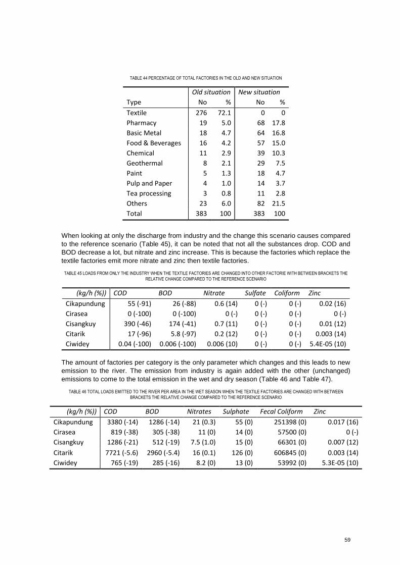
59
TABLE 44 PERCENTAGE OF TOTAL FACTORIES IN THE OLD AND NEW SITUATION
Old situation New situation
Type No % No %
Textile 276 72.1 0 0
Pharmacy 19 5.0 68 17.8
Basic Metal 18 4.7 64 16.8
Food & Beverages 16 4.2 57 15.0
Chemical 11 2.9 39 10.3
Geothermal 8 2.1 29 7.5
Paint 5 1.3 18 4.7
Pulp and Paper 4 1.0 14 3.7
Tea processing 3 0.8 11 2.8
Others 23 6.0 82 21.5
Total 383 100 383 100
When looking at only the discharge from industry and the change this scenario causes compared
to the reference scenario (Table 45), it can be noted that not all the substances drop. COD and
BOD decrease a lot, but nitrate and zinc increase. This is because the factories which replace the
textile factories emit more nitrate and zinc then textile factories.
TABLE 45 LOADS FROM ONLY THE INDUSTRY WHEN THE TEXTILE FACTORIES ARE CHANGED INTO OTHER FACTORIE WITH BETWEEN BRACKETS THE
RELATIVE CHANGE COMPARED TO THE REFERENCE SCENARIO
(kg/h (%)) COD BOD Nitrate Sulfate Coliform Zinc
Cikapundung 55 (-91) 26 (-88) 0.6 (14) 0 (-) 0 (-) 0.02 (16)
Cirasea 0 (-100) 0 (-100) 0 (-) 0 (-) 0 (-) 0 (-)
Cisangkuy 390 (-46) 174 (-41) 0.7 (11) 0 (-) 0 (-) 0.01 (12)
Citarik 17 (-96) 5.8 (-97) 0.2 (12) 0 (-) 0 (-) 0.003 (14)
Ciwidey 0.04 (-100) 0.006 (-100) 0.006 (10) 0 (-) 0 (-) 5.4E-05 (10)
The amount of factories per category is the only parameter which changes and this leads to new
emission to the river. The emission from industry is again added with the other (unchanged)
emissions to come to the total emission in the wet and dry season (Table 46 and Table 47).
TABLE 46 TOTAL LOADS EMITTED TO THE RIVER PER AREA IN THE WET SEASON WHEN THE TEXTILE FACTORIES ARE CHANGED WITH BETWEEN
BRACKETS THE RELATIVE CHANGE COMPARED TO THE REFERENCE SCENARIO
(kg/h (%)) COD BOD Nitrates Sulphate Fecal Coliform Zinc
Cikapundung 3380 (-14) 1286 (-14) 21 (0.3) 55 (0) 251398 (0) 0.017 (16)
Cirasea 819 (-38) 305 (-38) 11 (0) 14 (0) 57500 (0) 0 (-)
Cisangkuy 1286 (-21) 512 (-19) 7.5 (1.0) 15 (0) 66301 (0) 0.007 (12)
Citarik 7721 (-5.6) 2960 (-5.4) 16 (0.1) 126 (0) 606845 (0) 0.003 (14)
Ciwidey 765 (-19) 285 (-16) 8.2 (0) 13 (0) 53992 (0) 5.3E-05 (10)
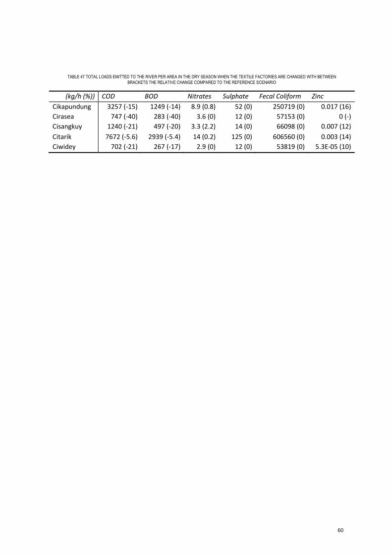
60
TABLE 47 TOTAL LOADS EMITTED TO THE RIVER PER AREA IN THE DRY SEASON WHEN THE TEXTILE FACTORIES ARE CHANGED WITH BETWEEN
BRACKETS THE RELATIVE CHANGE COMPARED TO THE REFERENCE SCENARIO
(kg/h (%)) COD BOD Nitrates Sulphate Fecal Coliform Zinc
Cikapundung 3257 (-15) 1249 (-14) 8.9 (0.8) 52 (0) 250719 (0) 0.017 (16)
Cirasea 747 (-40) 283 (-40) 3.6 (0) 12 (0) 57153 (0) 0 (-)
Cisangkuy 1240 (-21) 497 (-20) 3.3 (2.2) 14 (0) 66098 (0) 0.007 (12)
Citarik 7672 (-5.6) 2939 (-5.4) 14 (0.2) 125 (0) 606560 (0) 0.003 (14)
Ciwidey 702 (-21) 267 (-17) 2.9 (0) 12 (0) 53819 (0) 5.3E-05 (10)
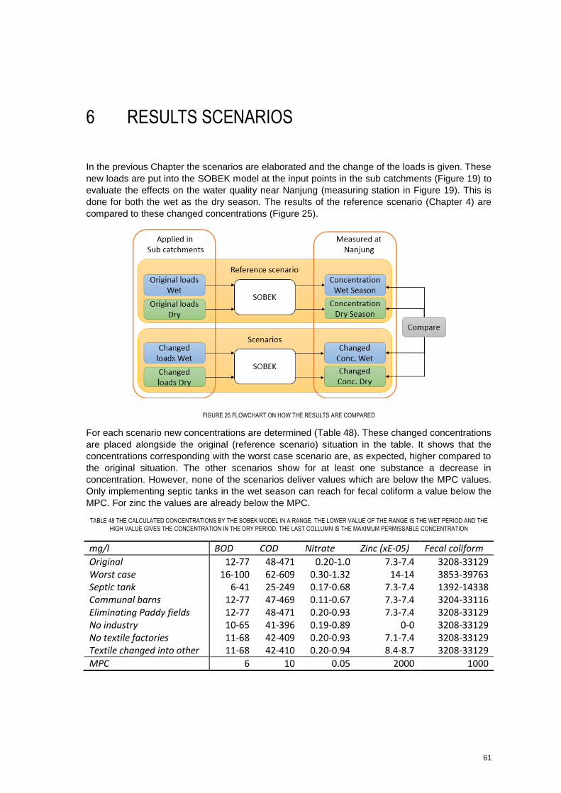
61
6 RESULTS SCENARIOS
In the previous Chapter the scenarios are elaborated and the change of the loads is given. These
new loads are put into the SOBEK model at the input points in the sub catchments (Figure 19) to
evaluate the effects on the water quality near Nanjung (measuring station in Figure 19). This is
done for both the wet as the dry season. The results of the reference scenario (Chapter 4) are
compared to these changed concentrations (Figure 25).
FIGURE 25 FLOWCHART ON HOW THE RESULTS ARE COMPARED
For each scenario new concentrations are determined (Table 48). These changed concentrations
are placed alongside the original (reference scenario) situation in the table. It shows that the
concentrations corresponding with the worst case scenario are, as expected, higher compared to
the original situation. The other scenarios show for at least one substance a decrease in
concentration. However, none of the scenarios deliver values which are below the MPC values.
Only implementing septic tanks in the wet season can reach for fecal coliform a value below the
MPC. For zinc the values are already below the MPC.
TABLE 48 THE CALCULATED CONCENTRATIONS BY THE SOBEK MODEL IN A RANGE. THE LOWER VALUE OF THE RANGE IS THE WET PERIOD AND THE
HIGH VALUE GIVES THE CONCENTRATION IN THE DRY PERIOD. THE LAST COLLUMN IS THE MAXIMUM PERMISSABLE CONCENTRATION
mg/l BOD COD Nitrate Zinc (xE-05) Fecal coliform
Original 12-77 48-471 0.20-1.0 7.3-7.4 3208-33129 Worst case 16-100 62-609 0.30-1.32 14-14 3853-39763 Septic tank 6-41 25-249 0.17-0.68 7.3-7.4 1392-14338 Communal barns 12-77 47-469 0.11-0.67 7.3-7.4 3204-33116 Eliminating Paddy fields 12-77 48-471 0.20-0.93 7.3-7.4 3208-33129 No industry 10-65 41-396 0.19-0.89 0-0 3208-33129 No textile factories 11-68 42-409 0.20-0.93 7.1-7.4 3208-33129 Textile changed into other 11-68 42-410 0.20-0.94 8.4-8.7 3208-33129
MPC 6 10 0.05 2000 1000
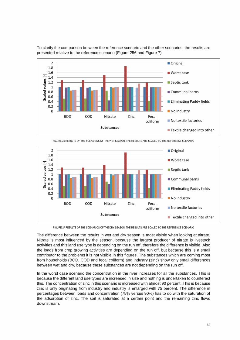
62
To clarify the comparison between the reference scenario and the other scenarios, the results are
presented relative to the reference scenario (Figure 256 and Figure 7).
FIGURE 25 RESULTS OF THE SCENARIOS OF THE WET SEASON. THE RESULTS ARE SCALED TO THE REFERENCE SCENARIO
FIGURE 27 RESULTS OF THE SCENARIOS OF THE DRY SEASON. THE RESULTS ARE SCALED TO THE REFERENCE SCENARIO
The difference between the results in wet and dry season is most visible when looking at nitrate.
Nitrate is most influenced by the season, because the largest producer of nitrate is livestock
activities and this land use type is depending on the run off, therefore the difference is visible. Also
the loads from crop growing activities are depending on the run off, but because this is a small
contributor to the problems it is not visible in this figures. The substances which are coming most
from households (BOD, COD and fecal coliform) and industry (zinc) show only small differences
between wet and dry, because these substances are not depending on the run off.
In the worst case scenario the concentration in the river increases for all the substances. This is
because the different land use types are increased in size and nothing is undertaken to counteract
this. The concentration of zinc in this scenario is increased with almost 90 percent. This is because
zinc is only originating from industry and industry is enlarged with 75 percent. The difference in
percentages between loads and concentration (75% versus 90%) has to do with the saturation of
the adsorption of zinc. The soil is saturated at a certain point and the remaining zinc flows
downstream.
00.20.40.60.8
11.21.41.61.8
2
BOD COD Nitrate Zinc Fecalcoliform
Scal
ed
val
ue
s [-
]
Substances
Original
Worst case
Septic tank
Communal barns
Eliminating Paddy fields
No industry
No textile factories
Textile changed into other
00.20.40.60.8
11.21.41.61.8
2
BOD COD Nitrate Zinc Fecalcoliform
Scal
ed
val
ue
s [-
]
Substances
Original
Worst case
Septic tank
Communal barns
Eliminating Paddy fields
No industry
No textile factories
Textile changed into other
63
Not only in the worst case have scenario substances increased. For the scenario where the textile
factories are changed into other industries, the concentration of zinc increases. The reason for this
is that textile factories, in this research, do not emit zinc. Zinc comes from the other industries in
the area. Increasing these industries logically leads to an increase in zinc.
The scenario with overall the best result is implementing septic tanks for the people who do not
have sanitation facilities. Nitrate is decreased a bit, BOD and COD are almost halved, and fecal
coliform even more as half. This large decrease is caused by the large amount of people present
in the area. Domestic is the largest contributor to the problem (Figure 18), so improving something
for this land use type should have a large effect on the concentration of the different substances
in the river. Zinc is in this scenario untouched, because people are not emitting zinc.
The scenario with the least impact involves agriculture (eliminating paddy fields). Agriculture is not
a large contributor to the pollution in the river (Figure 18) and the changes made lead also to very
low changes in the total loads (Table 37 and 38) so changing something in this land use type has
not a large effect on the improvement of the water quality.
64
7 DISCUSSION
The purpose of this research was to determine and calculate scenarios which give stakeholders
handhold on what measures have a large effect and which less. Because of the reliability of the
data and the amount of assumptions made, makes this research more a guideline then an
instruction. The scenarios have to be compared to the other scenarios and not with the measured
concentration.
In this chapter the important assumptions which have an influence on the input and outcome of
this research are discussed.
7.1 Substances
In this research only six substances are used. This because of the lack of data and modeling all
the substances would take a lot of time. Therefore only the most important substances are chosen,
which are also representative for the four land use types. By choosing only six substances the
processes among substances are limited. Some substances originate from a reaction between
other substances (ammonium and oxygen gives nitrate) and some react to new substances. Only
having this six substances limits the reactions between substances and therefore some
substances will be overestimated and other substances will be underestimated. This can be seen
in Table 25 where the calculated concentration of nitrate is lower than the measured concentration.
Nitrate is produced by oxidation of ammonium (nitrification), but ammonium is not included in this
model.
For the six substances the emission per land use type is determined. This is done by looking at
processes which take place within a land use type, however not all processes are considered. For
example the emission per person is taken into account for domestic, but substances coming from
the building materials of houses or vehicles is not. The same goes for industry. Here only the
processes within a factory are considered. The building which houses the factory is left out. This
causes that some substances are presented lower than in reality.
7.2 Measured concentration data
Measured data is used to determine the severity of the problem and to verify whether the outcome
of the model reliable is or not. In the comparison between the calculated concentration and the
measured concentration, data is used from PJT-II. This organization measures the water quality
once every month. The measured data therefore is in a moment of time. It is possible that the water
quality is, for some reason, at the moment of measuring, is worse or better as usual. This means
that the data which is used for the comparison can be an overestimation or underestimation. A
consequence of this is that the conclusion drawn in section 4.7 (the calculated outcome is within
the same order of magnitude and that enough confidence is given to model the scenarios) is based
on less reliable data. This does not change the outcome of the model, but changes the confidence
of the outcome.
7.3 Emission determination
Assumptions are made when determining the emission from the different land use types. These
assumptions are based on literature. The figures founds were based on other basins in the world
and the figures found on the Citarum Basin (as pointed out in chapter 4) can be doubted. A
subdivision is made to discuss the assumptions and which assumptions are more important in the
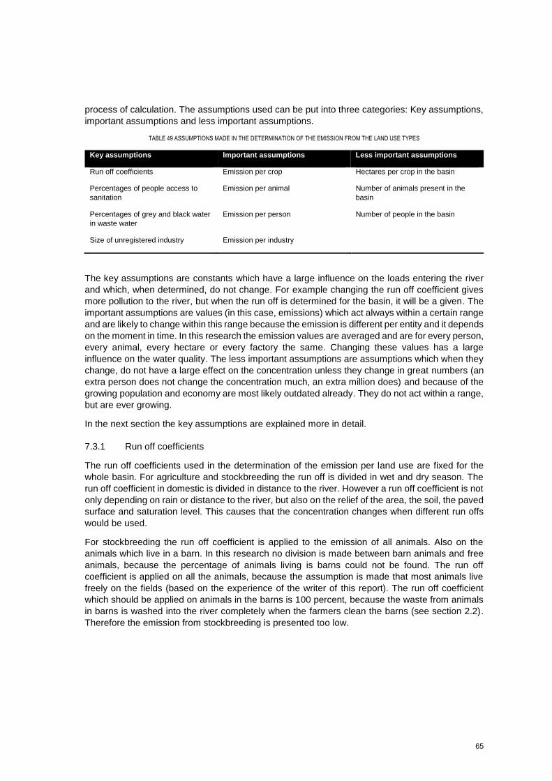
65
process of calculation. The assumptions used can be put into three categories: Key assumptions,
important assumptions and less important assumptions.
TABLE 49 ASSUMPTIONS MADE IN THE DETERMINATION OF THE EMISSION FROM THE LAND USE TYPES
Key assumptions Important assumptions Less important assumptions
Run off coefficients Emission per crop Hectares per crop in the basin
Percentages of people access to
sanitation
Emission per animal Number of animals present in the
basin
Percentages of grey and black water
in waste water
Emission per person Number of people in the basin
Size of unregistered industry Emission per industry
The key assumptions are constants which have a large influence on the loads entering the river
and which, when determined, do not change. For example changing the run off coefficient gives
more pollution to the river, but when the run off is determined for the basin, it will be a given. The
important assumptions are values (in this case, emissions) which act always within a certain range
and are likely to change within this range because the emission is different per entity and it depends
on the moment in time. In this research the emission values are averaged and are for every person,
every animal, every hectare or every factory the same. Changing these values has a large
influence on the water quality. The less important assumptions are assumptions which when they
change, do not have a large effect on the concentration unless they change in great numbers (an
extra person does not change the concentration much, an extra million does) and because of the
growing population and economy are most likely outdated already. They do not act within a range,
but are ever growing.
In the next section the key assumptions are explained more in detail.
7.3.1 Run off coefficients
The run off coefficients used in the determination of the emission per land use are fixed for the
whole basin. For agriculture and stockbreeding the run off is divided in wet and dry season. The
run off coefficient in domestic is divided in distance to the river. However a run off coefficient is not
only depending on rain or distance to the river, but also on the relief of the area, the soil, the paved
surface and saturation level. This causes that the concentration changes when different run offs
would be used.
For stockbreeding the run off coefficient is applied to the emission of all animals. Also on the
animals which live in a barn. In this research no division is made between barn animals and free
animals, because the percentage of animals living is barns could not be found. The run off
coefficient is applied on all the animals, because the assumption is made that most animals live
freely on the fields (based on the experience of the writer of this report). The run off coefficient
which should be applied on animals in the barns is 100 percent, because the waste from animals
in barns is washed into the river completely when the farmers clean the barns (see section 2.2).
Therefore the emission from stockbreeding is presented too low.
66
7.3.2 Sanitation accessibility
In the calculation of the emission from households some assumptions are made which relates to
sanitation:
- The access to sanitation is, in this research, depending on whether the people live in a city
or in a more rural environment. The assumption is made that in the city more people have
access to a sewage system.
- The waste water discharged by sewage systems is all treated and nothing is leaked to the
surface water.
- It is also assumed that all the septic tanks have the same leakage/spillage percentage of
40 percent.
- All waste water from people without any sanitation is directly discharged into the river.
These assumptions can be disputed because most of the sewage systems in Bandung are still
from the Dutch period (ADB, 2013), therefore rather old and a good change they are leaking. Not
all septic tanks leak that much or even more; and not all people without sanitation defecate in the
river. The emissions calculated in this research changes when assuming other values for the
percentages used.
7.3.3 Grey and black water
The division between grey and black water is based on data from developed countries. Indonesia
is a developing country. It is assumed that the less industrialized a country is, the less black water
(proportionally) a person produces. Less black water leads to less fecal coliform for example.
Because the large amount of people in the Citarum Basin, such an assumption can have large
influences on the water quality
7.3.4 Size unregistered industries
To determine the size of the unregistered industry, the assumption from the government is
adopted. However the way this assumption is made, is unknown and therefore the size is
questionable. A lot of the unregistered industries are home industries, like bakeries, sewing
workshops etc. The number is hard to guess. The land use ‘industry’ is a large polluter in some
areas and therefore changing the size of registered industries can have a large impact on the water
quality.
7.4 Model
In the SOBEK model a lot of parameters can be calibrated to represent the reality as good as
possible. For this research however all the parameters are kept on the default settings. This is
done because SOBEK is a very extensive program with a lot of complicated settings and calibrating
a model to come to a value comparable with a value which itself is also questionable, seems not
correct. The effect of adding the calibration and validation step to the process (when the data sets
are at disposal) is that the confidence of the outcome of the model is improved and that the
understanding of what is going on in the program is clarified.
The model is used to come to a concentration based on the emission determination done in this
research. This concentration value is then used as reference for the calculated concentrations with
the scenarios. This way the scenarios all have the same basis and with the same parameters the
conclusion stays the same when using a calibrated model.
67
7.5 Results
The results of this research are the outcomes of the scenarios in SOBEK. These results are
calculated with defaults settings of the model and the same assumptions as in the determination
of the reference scenario. Therefore the conclusions drawn on the results do not change when
changing some parameters, as long as they are changed for all scenarios.
The concentrations coming from the scenarios calculated at the end of 2015. The implementation
in the field of the measures used in the scenarios takes time. Before all the measures are
implemented the population, industry and agriculture are already increased. The effect of the
scenarios in reality are therefore smaller than predicted in this report.
68
8 CONCLUSIONS
The goal of this research was to determine and calculate scenario which give stakeholders a
handhold on what measures have a large effect and which less. This is done by developing
scenarios. These scenarios are based on alternative land use and water quality management as
suggested in interviews with involved stakeholders.
This final Chapter presents answers to the research questions based on the goal of this
research, as posed in chapter 1.
1. What are, according to the different authorities, the causes of and possible solutions for
the impaired water quality in the Citarum River? (Chapter 2)
Stakeholders
The stakeholders interviewed were people from the local, provincial and national government
which have authority on water quality; a non-governmental organization (NGO) which tries to raise
awareness of the problem in the Citarum River; and an organization for the water quality managers
of the industry. In the answers given by these stakeholders it was noted that the different
stakeholders gave apart from each other almost the same answers, therefore no distinction is
made between the different stakeholders.
Causes and solutions
Domestic waste is the largest polluter in the area, because of the number of people living in the
area. Not all people are connected to a sort of sanitation and dump their waste directly in the river
or on the lands. The waste water from people with a sanitation facility is not always fully treated.
The waste water treatment plants are old, septic tanks are leaking or are not emptied on time. The
solution is, easily said, building more waste water treatment plants, more connections to the
sewage systems and more septic tanks for the people in rural areas. The government should then
hire more truck drivers to empty the septic tanks.
For agriculture the problems were the scarcity of the land, which lead to the cultivation of the hills
and erosion, and the unfamiliarity of the farmers with fertilizers and pesticides. The latter makes
that farmers use too much of it or use it illegally. The solution to these problems is educating the
farmers on the use of fertilizers and pesticides, and planting perennial crops.
For stockbreeding the problems are the spreading of the animals throughout the basin. The
manure is not collected and washed directly into the river. Built biogas facilities do not work
because there are not enough animals near to keep it running and the people are not educated to
work with it. A solution to the problems is the relocation of animals into communal barns. The
manure can then easily be collected and used in the biogas facilities. Educating the farmers on the
usage of the facilities is then a logical consequence.
The industry in the Upper Citarum basin can be divided into registered and unregistered industry.
The registered industry is obliged to have treatment of the water, but this costs money and
therefore this is not always done. The government does not have enough inspectors to check all
the factories, so a lot of industries do not bother of treating their waste water. The unregistered
industries are small factories at people’s homes which are hard to detect and control. The solution
is more inspectors which enforce the law on waste water treatment and a centralized waste water
treatment plant, run by the government.
69
2. What are the estimated loads and resulting concentrations of the most relevant substances
to the Citarum River? (Chapter 3+4)
Based on the water quality data the most relevant substances to model are: Chemical Oxygen
Demand (COD), Biochemical Oxygen Demand (BOD), nitrate, sulphate, fecal coliform and zinc.
This also gives a representation of the different land uses. Unfortunately, sulphate cannot be
modelled in SOBEK, therefore it is not in the final calculations.
The loads of these substances are determined by estimating the load of a single unit per land use
type and adding the total as input to the SOBEK model to calculate the concentrations at the end
of the Upper Citarum Basin (Nanjung). The calculated loads show that domestic is by far the largest
polluter in the area for COD, BOD, fecal coliform and sulphate. Stockbreeding causes the highest
emission for nitrate. Zinc is an anomaly because it is only emitted by industry.
These concentrations are then compared to the measured concentrations to check whether the
estimations are accurate. In the comparison it shows that COD is overestimated, where nitrate and
zinc are underestimated. The results for BOD are in the wet season comparable with the measured
values, but are overestimated for the dry season. The deviation in the calculated compared to the
measured values has to do with the assumptions made. The amount of substances chosen; the
emission parameters change the input in the SOBEK model; the model parameters change the
outcome; and the amount of processes which determine the input values, all lead to a deviation
between the measured and calculated values.
Even though there are large uncertainties in the estimated loads and model assumptions
(discharge, processes, stationary), the model still produces concentrations in the same order of
magnitude as the measured concentrations.
3. What are suitable scenarios for the Citarum River Basin and the associated changes in
loads? (Chapter 5)
The interviews and the concentration data are used to determine a few scenarios. The scenarios
chosen are:
- Reference scenario
- Worst case scenario
- Improvement of sanitation
- Communal barns for the cattle
- Changing crops
- Changing industries
The scenarios represent changes in land use or taking action to reduce emission from a given type
of land use. The purpose of the scenarios is to lower the concentration of all the substances in the
river compared to the reference scenario. The exception is the worst case scenario. This has to
be a deterrent when no improvements are made, but the population and economy keeps on
growing. For the other scenarios goes that the water quality overall improves. Not all substances
change for each scenario, but mostly the associated concentration drops.
4. What are the most promising scenarios based on their effect on water quality? (Chapter
6)
Based on the effect of the water quality, giving septic tanks to people without any sanitation is the
most promising. This leads to the biggest drop for BOD, COD and fecal coliform. The biggest drop
in nitrate is when putting the cattle in communal barns. These scenarios are also relatively feasible,
because this can be enforced by the government where the other scenarios need more powerful
people involved (industries).
70
9 RECOMMENDATIONS
Based on this research multiple recommendations can be made. Recommendations for further
research as well for improving the model.
9.1 Further research
The assumptions made in this research are based on one source on the water quality in the Upper
Citarum basin and on literature of other basins in the world. The circumstances in the Upper
Citarum Basin are not always comparable to the areas used in the literature. Therefore more
research has to be done on the emissions from the different land uses in the Upper Citarum Basin
to verify the input of emissions.
- More data on the emission from the different industries
- Data on the emission and location of the unregistered industries
- More detailed information on the division of crops throughout the basin and the emission
in time
- More data in the application of fertilizers and pesticides in the basin
- The amount and location of animals throughout the basin
- Better prediction on the amount of people access to some sort of sanitation
- The spills in the sewage systems and septic tanks
9.2 Improving input for the model
The run off in this research is aligned for the whole basin. An improvement for the reliability of the
outcomes is the use of multiple run off coefficients for different areas of the basin (as pointed out
in the Discussion). Also a better division in domestic between city and rural is desirable. The
expectation is risen that some areas in the city are connected to the sewage system and others
are not. This leads that there is a different discharge of pollution for different areas in the city, unlike
is said in this research where the discharge from the city is aligned.
When more data from the different land uses and the different run off coefficients can be obtained,
it is possible to divide the area in smaller sub basins. In this research only five sub basins are taken
into account which each its own emission point. In the most idealized situation a model can be
build where at each segment in the river the concentration can be determined. Therefore a very
fine grid of emission points is needed and consequently more refined data. This all leads to a better
view on the impaired water quality and would hopefully increase the decisiveness to tackle the
problems.
9.3 Improving the model
In this research the parameters in the model are kept on their default settings. A
calibration/validation step is missing, because of the lack of data. A recommendation for improving
the model outcome is calibration and validation of the model. This leads to a more reliable outcome.
To do so more data on the concentration in the Citarum river is needed.
When it appears that not enough data is found to calibrate/validate the model, a simpler model
should be used. A simple model build in excel can also be a way to calculate the concentrations.
A comparison between the SOBEK model and an excel model is not done in this research.
Therefore this is a recommendation to investigate.

71
9.4 Scenarios
The scenarios show a decrease in concentrations at Nanjung, however not one scenario shows
values below the MPC. This means that the measures separately are not enough to improve the
water quality sufficiently. A recommendation is to combine the scenarios to look whether the water
quality drops below the maximum permissible concentration.
72
10 BIBLIOGRAPHY
Almy, F. M. (2008). Sustainability Assessment on Sanitation Systems for Low Income Urban Areas in Indonesia, 121.
ADB. (2013). Downstream Impacts of Water Pollution in the Upper Citarum River , West Java , Indonesia, (October).
Berenzen, N., Lentzen-Godding, A., Probst, M., Schulz, H., Schulz, R., & Liess, M. (2005). A comparison of predicted and measured levels of runoff-related pesticide concentrations in small lowland streams on a landscape level. Chemosphere, 58, 683–691. doi:10.1016/j.chemosphere.2004.05.009
Biisser, S., Nga, P. T., Moree, A., & Ante, N. V. (n.d.). CHARACTERISTICS AND QUANTITIES OF DOMESTIC WASTEWATER IN URBAN AND PERI-URBAN HOUSEHOLDS IN HANOI Key words : Back water , grey water , Hanoi , household , loads , wastewater . Background The wastewater flows in Vietnamese HHs ( HH ) are greywater from ki.
Bond, T., & Templeton, M. R. (2011). History and future of domestic biogas plants in the developing world. Energy for Sustainable Development, 15(4), 347–354. doi:10.1016/j.esd.2011.09.003
Campos, H. M., & Von Sperling, M. (1996). Estimation of domestic wastewater characteristics in a developing country based on socio-economic variables. Water Science and Technology. doi:10.1016/0273-1223(96)00558-6
Casanova, L. M., Gerba, C. P., & Karpiscak, M. (2001). Chemical and microbial characterization of household graywater. Journal of Environmental Science and Health. Part A, Toxic/hazardous Substances & Environmental Engineering, 36(4), 395–401. doi:10.1081/ESE-100103471
Collins, N.-A. (2009, October 27). ADB Gives Indonesia 500 Million Dollar to Clean Up World's
Dirtiest River. Voice of America.
Craswell, E. T., & Karjalainen, U. (1990). Recent research on fertilizer problems in Asian agriculture. Fertilizer Research, 26(Table 1), 243–248. doi:10.1007/BF01048762
Deltares. (2011). Volume 1 : Strategic Flood Management Strategy, 1(May).
Deltares. (2015). SOBEK D-Water Quality User Manual. Delft: Deltares.
EPA. (2015, 2 11). Human Health Benchmarks for Pesticides. Opgeroepen op 2 11, 2015, van
United States Environmental Protection Agency:
http://iaspub.epa.gov/apex/pesticides/f?p=HHBP:home
Fares, Y. R., & Yudianto, D. (2003). Assessment of hydrological characteristics in the upper Citarum catchment, West Java. River Basin Management Ii, 7(May), 165–176. Retrieved from <Go to ISI>://WOS:000184464000016
73
Feder, G., Murgai, R., & Quizon, J. (2008). “Investing in Farmers-The Impacts of Farmer Field Schools in Relation to Integrated Pest Management”-A Comment. World Development, 36(4), 2103–2106. doi:10.1016/j.worlddev.2008.04.011
French, D. (1986). Confronting an unsolvable problem: Deforestation in Malawi. World Development, 14, 531–540. doi:10.1016/0305-750X(86)90068-9
Fulazzaky, M. A., Hadimuljono, M. B., Tun, U., Onn, H., Pahat, B., & Baru, K. (2008). Evaluation of the suitability of Citarum river water for different uses. Water, 1–14.
Groenink, I., & Schuurman, J. (2014, july 7). Citarum: Een rivier van uitersten. Verspers, 10(13).
Hyde, W. F., & Seve, J. E. (1993). The economic role of wood products in tropical deforestation: the severe example of Malawi. Forest Ecology and Management, 57, 283–300. doi:10.1016/0378-1127(93)90178-P
Imhof, B., & Mühlemann, J. (2005). G Reywater Treatment on Household Level in Developing Countries –. Water, 98.
Iskandar. (2013). Inventarisasa & Identifikasi Sumber dan Beban Pencemaran Air. Pengelolaan
Kualitas Air, 50.
Keeney, D. R. (1973). The nitrogen cycle in sediment water systems. Environ Quality.
Konradsen, F., Van Der Hoek, W., Cole, D. C., Hutchinson, G., Daisley, H., Singh, S., & Eddleston, M. (2003). Reducing acute poisoning in developing countries - Options for restricting the availability of pesticides. Toxicology, 192, 249–261. doi:10.1016/S0300-483X(03)00339-1
Llewelyn, R. V., & Williams, J. R. (1996). Nonparametric analysis of technical, pure technical, and scale efficiencies for food crop production in East Java, Indonesia. Agricultural Economics, 15, 113–126. doi:10.1016/S0169-5150(96)01202-9
Mancini, J. L. (1978). Numerical estimates of coliform mortality rates under various conditions.
Journal Water pollution control Federation, 2477-2484.
Mangan, L. (2014, april 11). The World's Dirtiest River TV review - A visit to a paradise under
threat. The Guardian.
Martin, P., & Wheeler, D. (1995). The Industrial Pollution Projection System, (March).
Mcdowell, R. W., Sharpley, a. N., Condron, L. M., Haygarth, P. M., & Brookes, P. C. (2001). Processes controlling soil phosphorus release to runoff and implications for agricultural management. Nutrient Cycling in Agroecosystems, 59, 269–284. doi:10.1023/A:1014419206761
Ministerie van Verkeer en Waterstaat. (1998). Vierde Nota waterhuishouding
Regeringsbeslissing. Den Haag.
Nibbering, J. W. (1999). Tree planting on deforested farmlands, Sewu Hills, Java, Indonesia: Impact of economic and institutional changes. Agroforestry Systems, 46(1997), 65–82. doi:10.1023/A:1006202911928
74
Nilaparvata lugens,. (1996). Management, 41(314), 375–385.
Oberman, Raoul, & Dobbs, Richard, & Budiman, Arief, & Thompson, Fraser, & Rosee, M. (2012). The Archipelago Economy: Unleasing Indonesia’s Potential, (September), 1–116.
Parikesit, Takeuchi, K., Tsunekawa, a., & Abdoellah, O. S. (2005). Kebon tatangkalan: A disappearing agroforest in the Upper Citarum Watershed, West Java, Indonesia. Agroforestry Systems, 63, 171–182. doi:10.1007/s10457-004-1182-x
Partowijoto, B. H. A. (2006). Monitoring and studies on water quality in some rivers and related water bodies in indonesia, 6(February), 14–16.
Poor, C. J., & McDonnell, J. J. (2007). The effects of land use on stream nitrate dynamics. Journal of Hydrology, 332, 54–68. doi:10.1016/j.jhydrol.2006.06.022
Prihandrijanti, M., & Firdayati, M. (2011). Current Situation and Considerations of Domestic Waste- water Treatment Systems for Big Cities in Indonesia ( Case Study : Surabaya and Bandung ), 1(2), 97–104.
Sahu, N., Behera, S. K., Yamashiki, Y., Takara, K., & Yamagata, T. (2012). IOD and ENSO impacts on the extreme stream-flows of Citarum river in Indonesia. Climate Dynamics, 39, 1673–1680. doi:10.1007/s00382-011-1158-2
Sonzogni, W. C., Chesters, G., Coote, D. R., Konrad, J. C., Jeffs, D. N., Ostry, R. C., & Robinson, J. B. (1980). Pollution from land runoff. Environmental Science & Technology, 14(July 1978), 148–153. doi:10.1021/es60162a003
Sriwana, T., Van Bergen, M. J., Varekamp, J. C., Sumarti, S., Takano, B., Van Os, B. J. H., & Leng, M. J. (2000). Geochemistry of the acid Kawah Putih lake, Patuha Volcano, West Java, Indonesia. Journal of Volcanology and Geothermal Research, 97, 77–104. doi:10.1016/S0377-0273(99)00178-X
Sullivan, A. B., Snyder, D. M., & Rounds, S. A. (2010). Controls on biochemical oxygen demand
in the upper Kalmath River, Oregon. Elsevier. doi:doi:10.1016/j.chemgeo.2009.08.007
Sunarsih, S., Purwanto, P., & Budi, W. S. (2013). Management Efforts of Domestic Wastewater in Urban Based on Socio-Economic Variables. Environmental Management and Sustainable Development, 2(2), 29–40. doi:10.5296/emsd.v2i2.3668
Van den Berg, H., & Jiggins, J. (2007). Investing in Farmers - The Impacts of Farmer Field Schools in Relation to Integrated Pest Manangement. Elsevier, 35(4), 663–686.
Van Ginkel, C. H. (2015). Water quality of the Bandung Basin: towards a better understanding of the water quality of the Upper Citarum River Basin.
Widodo, T. W., Technos, C., Widodo, T. W., Tokumoto, O., & Office, T. (n.d.). SUGGESTION ON UTILIZATION OF FECES AT LARGE SCALE, 1–11.
Willis, H. (1983). Pesticides in Agricultural Runoff and Their, 1.
World Population Review. (2014). Indonesia Population 2014. Retrieved 1 21, 2015, from World Population Review: http://worldpopulationreview.com/countries/indonesia-population/
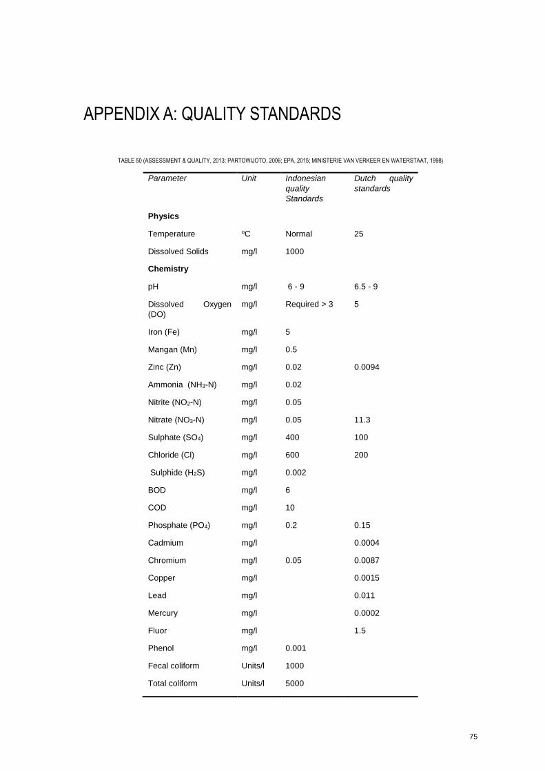
75
APPENDIX A: QUALITY STANDARDS
TABLE 50 (ASSESSMENT & QUALITY, 2013; PARTOWIJOTO, 2006; EPA, 2015; MINISTERIE VAN VERKEER EN WATERSTAAT, 1998)
Parameter Unit Indonesian
quality
Standards
Dutch quality
standards
Physics
Temperature oC Normal 25
Dissolved Solids mg/l 1000
Chemistry
pH mg/l 6 - 9 6.5 - 9
Dissolved Oxygen
(DO)
mg/l Required > 3 5
Iron (Fe) mg/l 5
Mangan (Mn) mg/l 0.5
Zinc (Zn) mg/l 0.02 0.0094
Ammonia (NH3-N) mg/l 0.02
Nitrite (NO2-N) mg/l 0.05
Nitrate (NO3-N) mg/l 0.05 11.3
Sulphate (SO4) mg/l 400 100
Chloride (Cl) mg/l 600 200
Sulphide (H2S) mg/l 0.002
BOD mg/l 6
COD mg/l 10
Phosphate (PO4) mg/l 0.2 0.15
Cadmium mg/l 0.0004
Chromium mg/l 0.05 0.0087
Copper mg/l 0.0015
Lead mg/l 0.011
Mercury mg/l 0.0002
Fluor mg/l 1.5
Phenol mg/l 0.001
Fecal coliform Units/l 1000
Total coliform Units/l 5000
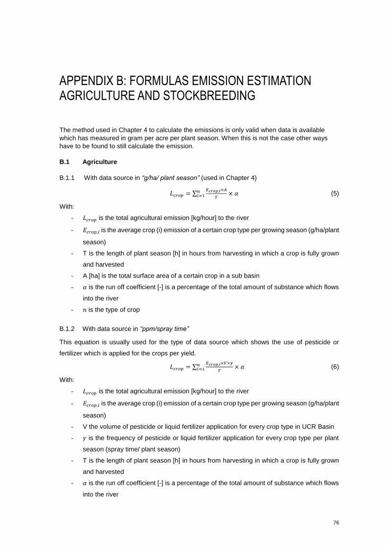
76
APPENDIX B: FORMULAS EMISSION ESTIMATION AGRICULTURE AND STOCKBREEDING
The method used in Chapter 4 to calculate the emissions is only valid when data is available
which has measured in gram per acre per plant season. When this is not the case other ways
have to be found to still calculate the emission.
B.1 Agriculture
B.1.1 With data source in “g/ha/ plant season” (used in Chapter 4)
𝐿𝑐𝑟𝑜𝑝 = ∑𝐸𝑐𝑟𝑜𝑝,𝑖×𝐴
𝑇× 𝛼 𝑛
𝑖=1 (5)
With:
- 𝐿𝑐𝑟𝑜𝑝 is the total agricultural emission [kg/hour] to the river
- 𝐸𝑐𝑟𝑜𝑝,𝑖 is the average crop (i) emission of a certain crop type per growing season (g/ha/plant
season)
- T is the length of plant season [h] in hours from harvesting in which a crop is fully grown
and harvested
- A [ha] is the total surface area of a certain crop in a sub basin
- 𝛼 is the run off coefficient [-] is a percentage of the total amount of substance which flows
into the river
- 𝑛 is the type of crop
B.1.2 With data source in “ppm/spray time”
This equation is usually used for the type of data source which shows the use of pesticide or
fertilizer which is applied for the crops per yield.
𝐿𝑐𝑟𝑜𝑝 = ∑𝐸𝑐𝑟𝑜𝑝,𝑖×𝑉×𝛾
𝑇× 𝛼 𝑛
𝑖=1 (6)
With:
- 𝐿𝑐𝑟𝑜𝑝 is the total agricultural emission [kg/hour] to the river
- 𝐸𝑐𝑟𝑜𝑝,𝑖 is the average crop (i) emission of a certain crop type per growing season (g/ha/plant
season)
- V the volume of pesticide or liquid fertilizer application for every crop type in UCR Basin
- 𝛾 is the frequency of pesticide or liquid fertilizer application for every crop type per plant
season (spray time/ plant season)
- T is the length of plant season [h] in hours from harvesting in which a crop is fully grown
and harvested
- 𝛼 is the run off coefficient [-] is a percentage of the total amount of substance which flows
into the river
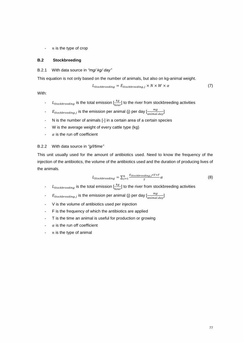
77
- 𝑛 is the type of crop
B.2 Stockbreeding
B.2.1 With data source in “mg/ kg/ day”
This equation is not only based on the number of animals, but also on kg-animal weight.
𝐿𝑆𝑡𝑜𝑐𝑘𝑏𝑟𝑒𝑒𝑑𝑖𝑛𝑔 = 𝐸𝑆𝑡𝑜𝑐𝑘𝑏𝑟𝑒𝑒𝑑𝑖𝑛𝑔,𝑗 × 𝑁 × 𝑊 × 𝛼 (7)
With:
- 𝐿𝑆𝑡𝑜𝑐𝑘𝑏𝑟𝑒𝑒𝑑𝑖𝑛𝑔 is the total emission [𝑘𝑔
ℎ𝑜𝑢𝑟] to the river from stockbreeding activities
- 𝐸𝑆𝑡𝑜𝑐𝑘𝑏𝑟𝑒𝑒𝑑𝑖𝑛𝑔,𝑗 is the emission per animal (j) per day [𝑚𝑔
𝑎𝑛𝑖𝑚𝑎𝑙.𝑑𝑎𝑦]
- N is the number of animals [-] in a certain area of a certain species
- W is the average weight of every cattle type (kg)
- 𝛼 is the run off coefficient
B.2.2 With data source in “g/l/time”
This unit usually used for the amount of antibiotics used. Need to know the frequency of the
injection of the antibiotics, the volume of the antibiotics used and the duration of producing lives of
the animals.
𝐿𝑆𝑡𝑜𝑐𝑘𝑏𝑟𝑒𝑒𝑑𝑖𝑛𝑔 = ∑𝐸𝑆𝑡𝑜𝑐𝑘𝑏𝑟𝑒𝑒𝑑𝑖𝑛𝑔,𝑗×𝑉×𝐹
𝑇𝛼 𝑛
𝑗=1 (8)
- 𝐿𝑆𝑡𝑜𝑐𝑘𝑏𝑟𝑒𝑒𝑑𝑖𝑛𝑔 is the total emission [𝑘𝑔
ℎ𝑜𝑢𝑟] to the river from stockbreeding activities
- 𝐸𝑆𝑡𝑜𝑐𝑘𝑏𝑟𝑒𝑒𝑑𝑖𝑛𝑔,𝑗 is the emission per animal (j) per day [𝑚𝑔
𝑎𝑛𝑖𝑚𝑎𝑙.𝑑𝑎𝑦]
- V is the volume of antibiotics used per injection
- F is the frequency of which the antibiotics are applied
- T is the time an animal is useful for production or growing
- 𝛼 is the run off coefficient
- 𝑛 is the type of animal
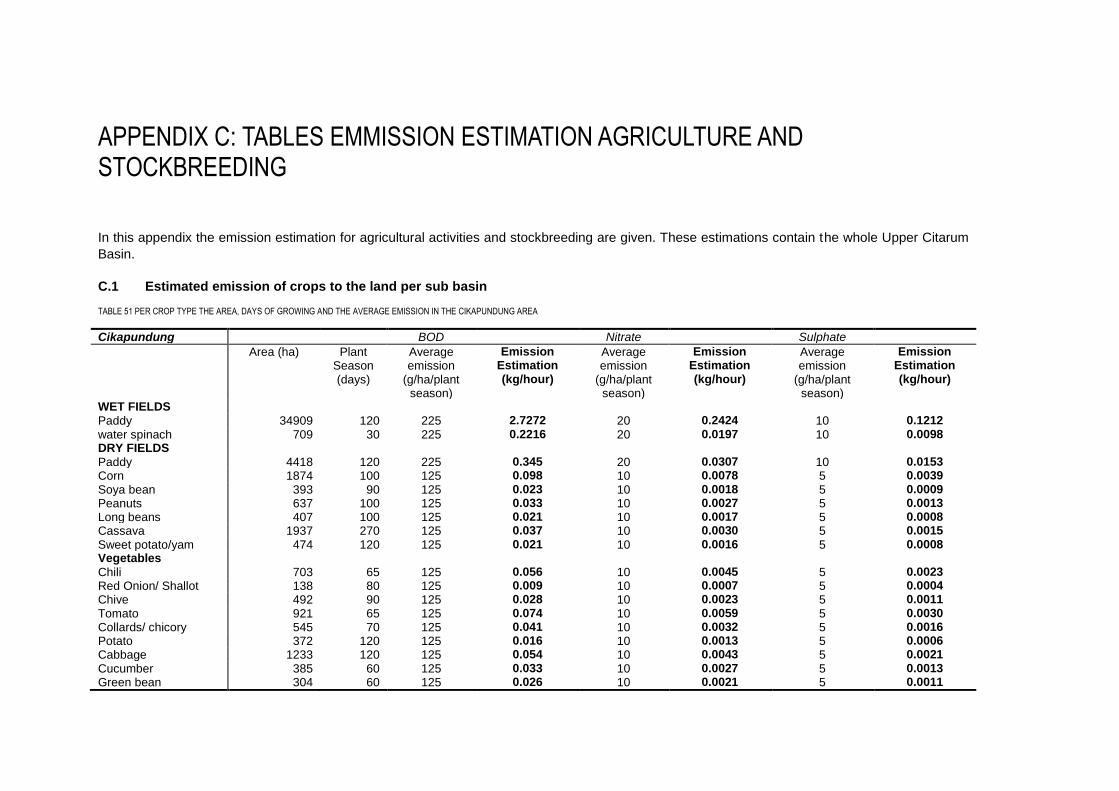
APPENDIX C: TABLES EMMISSION ESTIMATION AGRICULTURE AND STOCKBREEDING
In this appendix the emission estimation for agricultural activities and stockbreeding are given. These estimations contain the whole Upper Citarum
Basin.
C.1 Estimated emission of crops to the land per sub basin
TABLE 51 PER CROP TYPE THE AREA, DAYS OF GROWING AND THE AVERAGE EMISSION IN THE CIKAPUNDUNG AREA
Cikapundung BOD Nitrate Sulphate
Area (ha) Plant Season (days)
Average emission
(g/ha/plant season)
Emission Estimation (kg/hour)
Average emission
(g/ha/plant season)
Emission Estimation (kg/hour)
Average emission
(g/ha/plant season)
Emission Estimation (kg/hour)
WET FIELDS
Paddy 34909 120 225 2.7272 20 0.2424 10 0.1212
water spinach 709 30 225 0.2216 20 0.0197 10 0.0098 DRY FIELDS
Paddy 4418 120 225 0.345 20 0.0307 10 0.0153
Corn 1874 100 125 0.098 10 0.0078 5 0.0039
Soya bean 393 90 125 0.023 10 0.0018 5 0.0009
Peanuts 637 100 125 0.033 10 0.0027 5 0.0013
Long beans 407 100 125 0.021 10 0.0017 5 0.0008
Cassava 1937 270 125 0.037 10 0.0030 5 0.0015
Sweet potato/yam 474 120 125 0.021 10 0.0016 5 0.0008 Vegetables
Chili 703 65 125 0.056 10 0.0045 5 0.0023
Red Onion/ Shallot 138 80 125 0.009 10 0.0007 5 0.0004
Chive 492 90 125 0.028 10 0.0023 5 0.0011
Tomato 921 65 125 0.074 10 0.0059 5 0.0030
Collards/ chicory 545 70 125 0.041 10 0.0032 5 0.0016
Potato 372 120 125 0.016 10 0.0013 5 0.0006
Cabbage 1233 120 125 0.054 10 0.0043 5 0.0021
Cucumber 385 60 125 0.033 10 0.0027 5 0.0013
Green bean 304 60 125 0.026 10 0.0021 5 0.0011
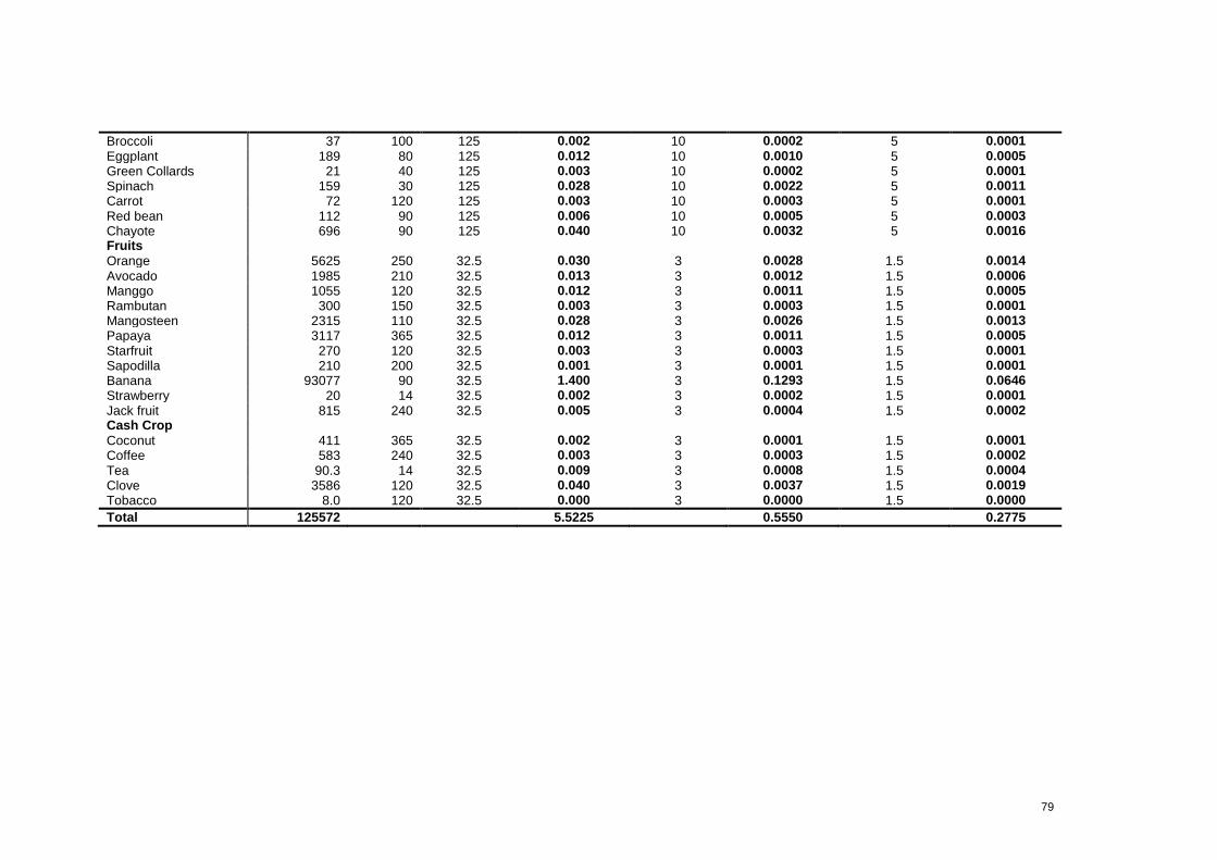
79
Broccoli 37 100 125 0.002 10 0.0002 5 0.0001
Eggplant 189 80 125 0.012 10 0.0010 5 0.0005
Green Collards 21 40 125 0.003 10 0.0002 5 0.0001
Spinach 159 30 125 0.028 10 0.0022 5 0.0011
Carrot 72 120 125 0.003 10 0.0003 5 0.0001
Red bean 112 90 125 0.006 10 0.0005 5 0.0003
Chayote 696 90 125 0.040 10 0.0032 5 0.0016 Fruits
Orange 5625 250 32.5 0.030 3 0.0028 1.5 0.0014
Avocado 1985 210 32.5 0.013 3 0.0012 1.5 0.0006
Manggo 1055 120 32.5 0.012 3 0.0011 1.5 0.0005
Rambutan 300 150 32.5 0.003 3 0.0003 1.5 0.0001
Mangosteen 2315 110 32.5 0.028 3 0.0026 1.5 0.0013
Papaya 3117 365 32.5 0.012 3 0.0011 1.5 0.0005
Starfruit 270 120 32.5 0.003 3 0.0003 1.5 0.0001
Sapodilla 210 200 32.5 0.001 3 0.0001 1.5 0.0001
Banana 93077 90 32.5 1.400 3 0.1293 1.5 0.0646
Strawberry 20 14 32.5 0.002 3 0.0002 1.5 0.0001
Jack fruit 815 240 32.5 0.005 3 0.0004 1.5 0.0002 Cash Crop
Coconut 411 365 32.5 0.002 3 0.0001 1.5 0.0001
Coffee 583 240 32.5 0.003 3 0.0003 1.5 0.0002
Tea 90.3 14 32.5 0.009 3 0.0008 1.5 0.0004
Clove 3586 120 32.5 0.040 3 0.0037 1.5 0.0019
Tobacco 8.0 120 32.5 0.000 3 0.0000 1.5 0.0000
Total 125572 5.5225 0.5550 0.2775
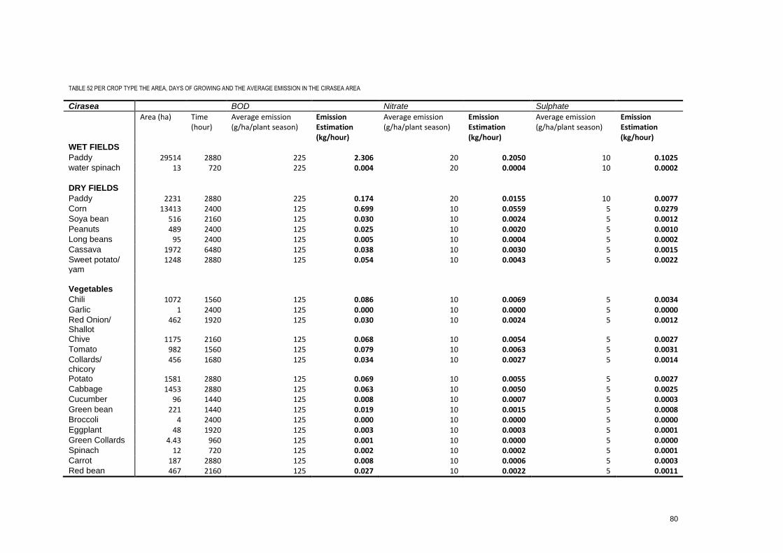
80
TABLE 52 PER CROP TYPE THE AREA, DAYS OF GROWING AND THE AVERAGE EMISSION IN THE CIRASEA AREA
Cirasea BOD Nitrate Sulphate
Area (ha) Time (hour)
Average emission (g/ha/plant season)
Emission Estimation (kg/hour)
Average emission (g/ha/plant season)
Emission Estimation (kg/hour)
Average emission (g/ha/plant season)
Emission Estimation (kg/hour)
WET FIELDS Paddy 29514 2880 225 2.306 20 0.2050 10 0.1025 water spinach 13 720 225 0.004 20 0.0004 10 0.0002 DRY FIELDS Paddy 2231 2880 225 0.174 20 0.0155 10 0.0077 Corn 13413 2400 125 0.699 10 0.0559 5 0.0279 Soya bean 516 2160 125 0.030 10 0.0024 5 0.0012 Peanuts 489 2400 125 0.025 10 0.0020 5 0.0010 Long beans 95 2400 125 0.005 10 0.0004 5 0.0002 Cassava 1972 6480 125 0.038 10 0.0030 5 0.0015 Sweet potato/ yam
1248 2880 125 0.054 10 0.0043 5 0.0022
Vegetables Chili 1072 1560 125 0.086 10 0.0069 5 0.0034 Garlic 1 2400 125 0.000 10 0.0000 5 0.0000 Red Onion/ Shallot
462 1920 125 0.030 10 0.0024 5 0.0012
Chive 1175 2160 125 0.068 10 0.0054 5 0.0027 Tomato 982 1560 125 0.079 10 0.0063 5 0.0031 Collards/ chicory
456 1680 125 0.034 10 0.0027 5 0.0014
Potato 1581 2880 125 0.069 10 0.0055 5 0.0027 Cabbage 1453 2880 125 0.063 10 0.0050 5 0.0025 Cucumber 96 1440 125 0.008 10 0.0007 5 0.0003 Green bean 221 1440 125 0.019 10 0.0015 5 0.0008 Broccoli 4 2400 125 0.000 10 0.0000 5 0.0000 Eggplant 48 1920 125 0.003 10 0.0003 5 0.0001 Green Collards 4.43 960 125 0.001 10 0.0000 5 0.0000 Spinach 12 720 125 0.002 10 0.0002 5 0.0001 Carrot 187 2880 125 0.008 10 0.0006 5 0.0003 Red bean 467 2160 125 0.027 10 0.0022 5 0.0011
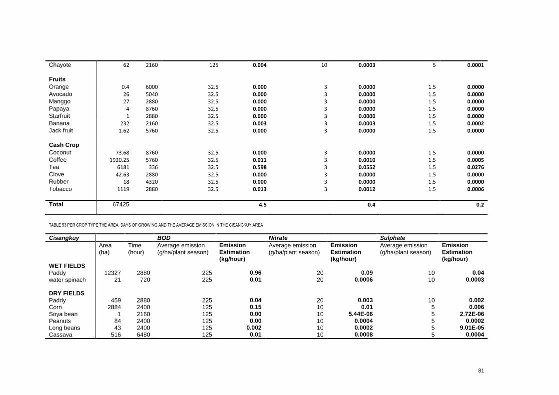
81
Chayote 62 2160 125 0.004 10 0.0003 5 0.0001 Fruits Orange 0.4 6000 32.5 0.000 3 0.0000 1.5 0.0000 Avocado 26 5040 32.5 0.000 3 0.0000 1.5 0.0000 Manggo 27 2880 32.5 0.000 3 0.0000 1.5 0.0000 Papaya 4 8760 32.5 0.000 3 0.0000 1.5 0.0000 Starfruit 1 2880 32.5 0.000 3 0.0000 1.5 0.0000 Banana 232 2160 32.5 0.003 3 0.0003 1.5 0.0002 Jack fruit 1.62 5760 32.5 0.000 3 0.0000 1.5 0.0000 Cash Crop Coconut 73.68 8760 32.5 0.000 3 0.0000 1.5 0.0000 Coffee 1920.25 5760 32.5 0.011 3 0.0010 1.5 0.0005 Tea 6181 336 32.5 0.598 3 0.0552 1.5 0.0276 Clove 42.63 2880 32.5 0.000 3 0.0000 1.5 0.0000 Rubber 18 4320 32.5 0.000 3 0.0000 1.5 0.0000 Tobacco 1119 2880 32.5 0.013 3 0.0012 1.5 0.0006
Total 67425 4.5 0.4 0.2
TABLE 53 PER CROP TYPE THE AREA, DAYS OF GROWING AND THE AVERAGE EMISSION IN THE CISANGKUY AREA
Cisangkuy BOD Nitrate Sulphate
Area (ha)
Time (hour)
Average emission (g/ha/plant season)
Emission Estimation (kg/hour)
Average emission (g/ha/plant season)
Emission Estimation (kg/hour)
Average emission (g/ha/plant season)
Emission Estimation (kg/hour)
WET FIELDS
Paddy 12327 2880 225 0.96 20 0.09 10 0.04
water spinach 21 720 225 0.01 20 0.0006 10 0.0003
DRY FIELDS
Paddy 459 2880 225 0.04 20 0.003 10 0.002
Corn 2884 2400 125 0.15 10 0.01 5 0.006
Soya bean 1 2160 125 0.00 10 5.44E-06 5 2.72E-06
Peanuts 84 2400 125 0.00 10 0.0004 5 0.0002
Long beans 43 2400 125 0.002 10 0.0002 5 9.01E-05
Cassava 516 6480 125 0.01 10 0.0008 5 0.0004
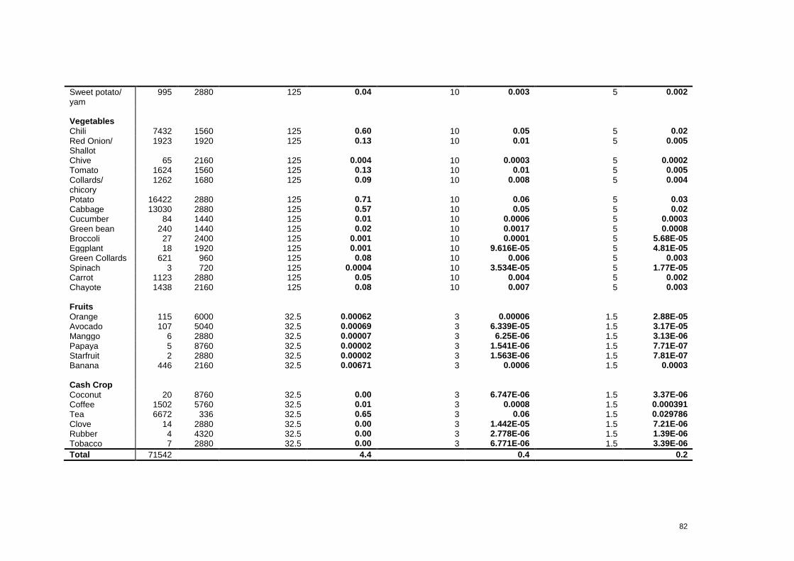
82
Sweet potato/ yam
995 2880 125 0.04 10 0.003 5 0.002
Vegetables
Chili 7432 1560 125 0.60 10 0.05 5 0.02
Red Onion/ Shallot
1923 1920 125 0.13 10 0.01 5 0.005
Chive 65 2160 125 0.004 10 0.0003 5 0.0002
Tomato 1624 1560 125 0.13 10 0.01 5 0.005
Collards/ chicory
1262 1680 125 0.09 10 0.008 5 0.004
Potato 16422 2880 125 0.71 10 0.06 5 0.03
Cabbage 13030 2880 125 0.57 10 0.05 5 0.02
Cucumber 84 1440 125 0.01 10 0.0006 5 0.0003
Green bean 240 1440 125 0.02 10 0.0017 5 0.0008
Broccoli 27 2400 125 0.001 10 0.0001 5 5.68E-05
Eggplant 18 1920 125 0.001 10 9.616E-05 5 4.81E-05
Green Collards 621 960 125 0.08 10 0.006 5 0.003
Spinach 3 720 125 0.0004 10 3.534E-05 5 1.77E-05
Carrot 1123 2880 125 0.05 10 0.004 5 0.002
Chayote 1438 2160 125 0.08 10 0.007 5 0.003
Fruits
Orange 115 6000 32.5 0.00062 3 0.00006 1.5 2.88E-05
Avocado 107 5040 32.5 0.00069 3 6.339E-05 1.5 3.17E-05
Manggo 6 2880 32.5 0.00007 3 6.25E-06 1.5 3.13E-06
Papaya 5 8760 32.5 0.00002 3 1.541E-06 1.5 7.71E-07
Starfruit 2 2880 32.5 0.00002 3 1.563E-06 1.5 7.81E-07
Banana 446 2160 32.5 0.00671 3 0.0006 1.5 0.0003
Cash Crop
Coconut 20 8760 32.5 0.00 3 6.747E-06 1.5 3.37E-06
Coffee 1502 5760 32.5 0.01 3 0.0008 1.5 0.000391
Tea 6672 336 32.5 0.65 3 0.06 1.5 0.029786
Clove 14 2880 32.5 0.00 3 1.442E-05 1.5 7.21E-06
Rubber 4 4320 32.5 0.00 3 2.778E-06 1.5 1.39E-06
Tobacco 7 2880 32.5 0.00 3 6.771E-06 1.5 3.39E-06
Total 71542 4.4 0.4 0.2
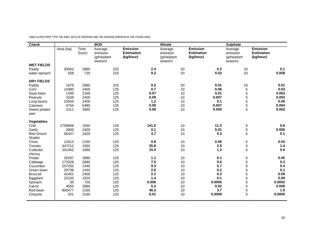
83
TABLE 54 PER CROP TYPE THE AREA, DAYS OF GROWING AND THE AVERAGE EMISSION IN THE CITARIK AREA
Citarik BOD Nitrate Sulphate
Area (ha) Time (hour)
Average emission (g/ha/plant season)
Emission Estimation (kg/hour)
Average emission (g/ha/plant season)
Emission Estimation (kg/hour)
Average emission (g/ha/plant season)
Emission Estimation (kg/hour)
WET FIELDS
Paddy 30563 2880 225 2.4 20 0.2 10 0.1
water spinach 558 720 225 0.2 20 0.02 10 0.008
DRY FIELDS
Paddy 1979 2880 225 0.2 20 0.01 10 0.01
Corn 14380 2400 125 0.7 10 0.06 5 0.03
Soya bean 1295 2160 125 0.07 10 0.01 5 0.003
Peanuts 1639 2400 125 0.09 10 0.007 5 0.003
Long beans 23504 2400 125 1.2 10 0.1 5 0.05
Cassava 4754 6480 125 0.09 10 0.007 5 0.004
Sweet potato/ yam
1411 2880 125 0.06 10 0.005 5 0.002
Vegetables
Chili 1759848 1560 125 141.0 10 11.3 5 5.6
Garlic 2800 2400 125 0.1 10 0.01 5 0.006
Red Onion/ Shallot
56347 1920 125 3.7 10 0.3 5 0.1
Chive 13413 2160 125 0.8 10 0.06 5 0.03
Tomato 447212 1560 125 35.8 10 2.9 5 1.4
Collards/ chicory
201462 1680 125 15.0 10 1.2 5 0.6
Potato 26297 2880 125 1.1 10 0.1 5 0.05
Cabbage 173328 2880 125 7.5 10 0.6 5 0.3
Cucumber 107252 1440 125 9.3 10 0.7 5 0.4
Green bean 29738 1440 125 2.6 10 0.2 5 0.1
Broccoli 42401 2400 125 2.2 10 0.2 5 0.09
Eggplant 22150 1920 125 1.4 10 0.1 5 0.06
Spinach 35 720 125 0.006 10 0.0005 5 0.0002
Carrot 4555 2880 125 0.2 10 0.02 5 0.008
Red bean 800477 2160 125 46.3 10 3.7 5 1.9
Chayote 201 2160 125 0.01 10 0.0009 5 0.0005
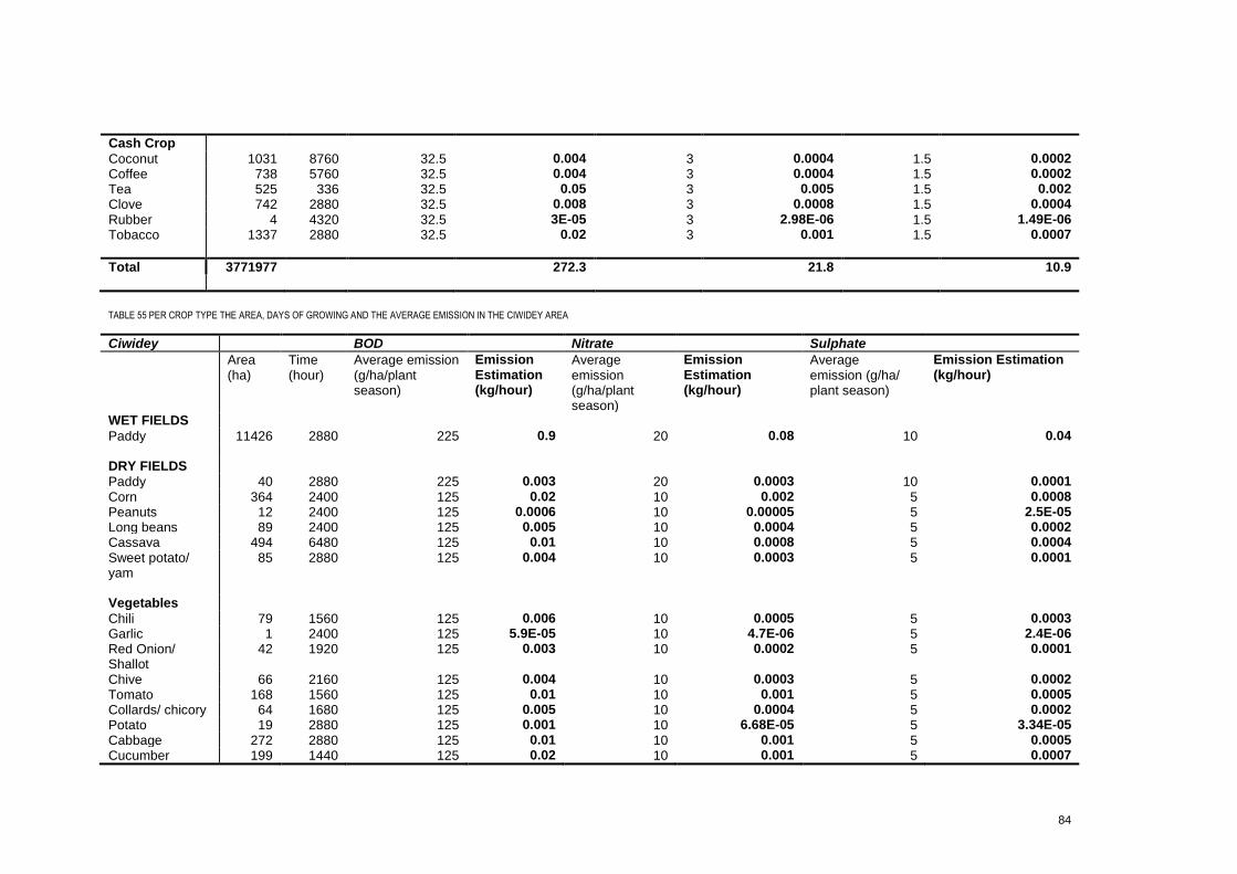
84
Cash Crop
Coconut 1031 8760 32.5 0.004 3 0.0004 1.5 0.0002
Coffee 738 5760 32.5 0.004 3 0.0004 1.5 0.0002
Tea 525 336 32.5 0.05 3 0.005 1.5 0.002
Clove 742 2880 32.5 0.008 3 0.0008 1.5 0.0004
Rubber 4 4320 32.5 3E-05 3 2.98E-06 1.5 1.49E-06
Tobacco 1337 2880 32.5 0.02 3 0.001 1.5 0.0007
Total 3771977 272.3 21.8 10.9
TABLE 55 PER CROP TYPE THE AREA, DAYS OF GROWING AND THE AVERAGE EMISSION IN THE CIWIDEY AREA
Ciwidey BOD Nitrate Sulphate
Area (ha)
Time (hour)
Average emission (g/ha/plant season)
Emission Estimation (kg/hour)
Average emission (g/ha/plant season)
Emission Estimation (kg/hour)
Average emission (g/ha/ plant season)
Emission Estimation (kg/hour)
WET FIELDS
Paddy 11426 2880 225 0.9 20 0.08 10 0.04
DRY FIELDS
Paddy 40 2880 225 0.003 20 0.0003 10 0.0001
Corn 364 2400 125 0.02 10 0.002 5 0.0008
Peanuts 12 2400 125 0.0006 10 0.00005 5 2.5E-05
Long beans 89 2400 125 0.005 10 0.0004 5 0.0002
Cassava 494 6480 125 0.01 10 0.0008 5 0.0004
Sweet potato/ yam
85 2880 125 0.004 10 0.0003 5 0.0001
Vegetables
Chili 79 1560 125 0.006 10 0.0005 5 0.0003
Garlic 1 2400 125 5.9E-05 10 4.7E-06 5 2.4E-06
Red Onion/ Shallot
42 1920 125 0.003 10 0.0002 5 0.0001
Chive 66 2160 125 0.004 10 0.0003 5 0.0002
Tomato 168 1560 125 0.01 10 0.001 5 0.0005
Collards/ chicory 64 1680 125 0.005 10 0.0004 5 0.0002
Potato 19 2880 125 0.001 10 6.68E-05 5 3.34E-05
Cabbage 272 2880 125 0.01 10 0.001 5 0.0005
Cucumber 199 1440 125 0.02 10 0.001 5 0.0007
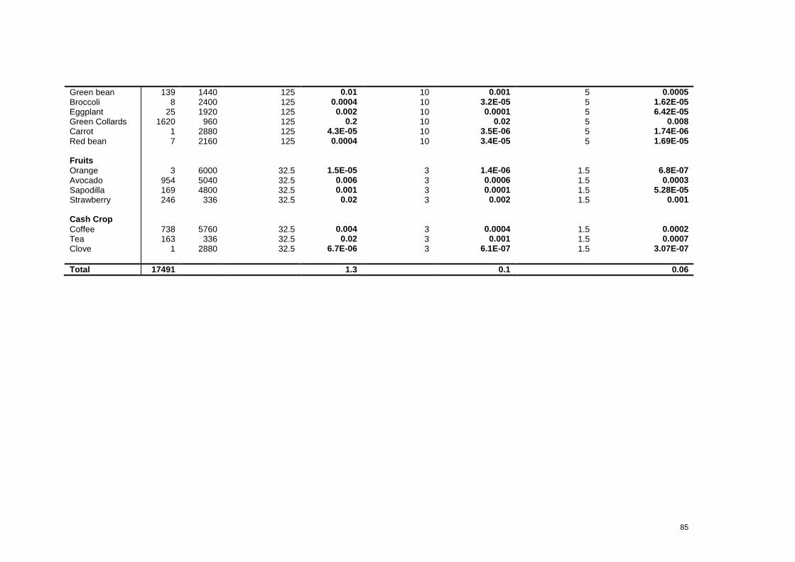
85
Green bean 139 1440 125 0.01 10 0.001 5 0.0005
Broccoli 8 2400 125 0.0004 10 3.2E-05 5 1.62E-05
Eggplant 25 1920 125 0.002 10 0.0001 5 6.42E-05
Green Collards 1620 960 125 0.2 10 0.02 5 0.008
Carrot 1 2880 125 4.3E-05 10 3.5E-06 5 1.74E-06
Red bean 7 2160 125 0.0004 10 3.4E-05 5 1.69E-05
Fruits
Orange 3 6000 32.5 1.5E-05 3 1.4E-06 1.5 6.8E-07
Avocado 954 5040 32.5 0.006 3 0.0006 1.5 0.0003
Sapodilla 169 4800 32.5 0.001 3 0.0001 1.5 5.28E-05
Strawberry 246 336 32.5 0.02 3 0.002 1.5 0.001
Cash Crop
Coffee 738 5760 32.5 0.004 3 0.0004 1.5 0.0002
Tea 163 336 32.5 0.02 3 0.001 1.5 0.0007
Clove 1 2880 32.5 6.7E-06 3 6.1E-07 1.5 3.07E-07
Total 17491 1.3 0.1 0.06
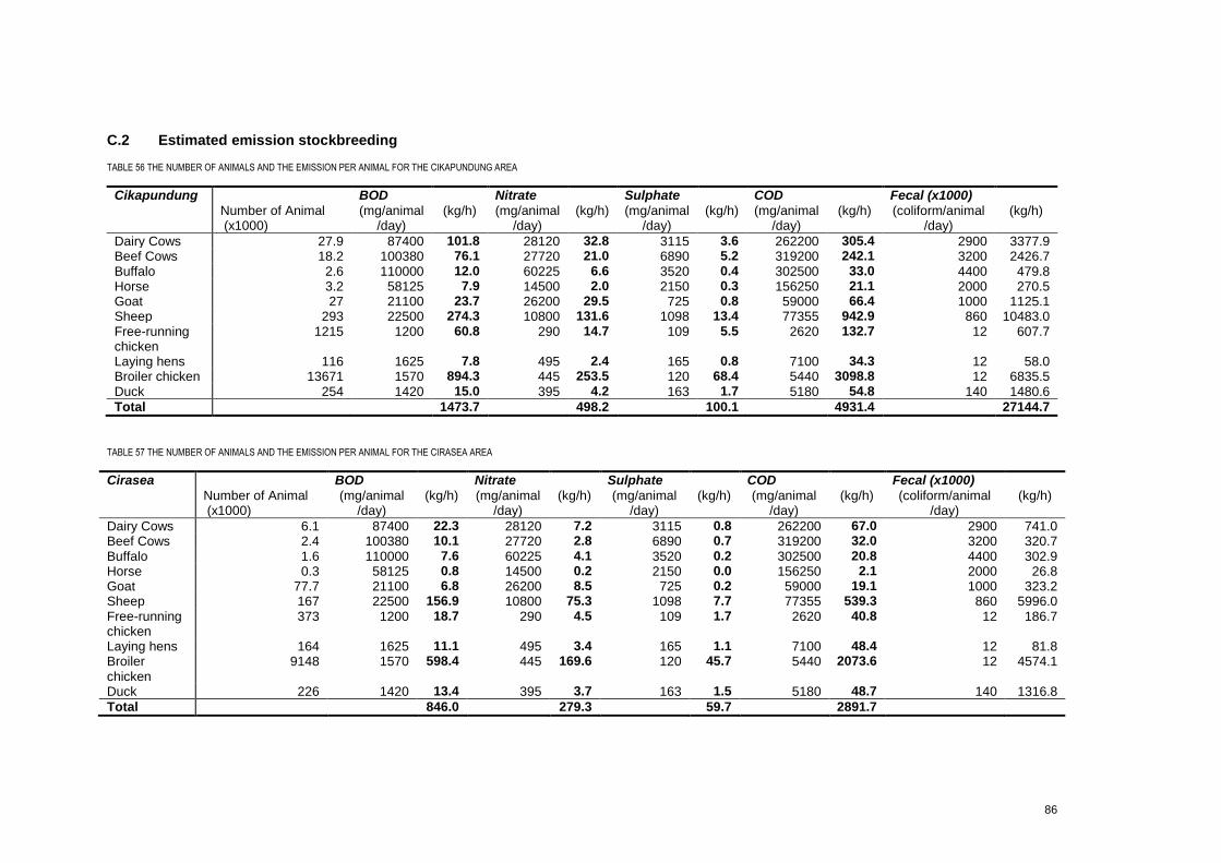
86
C.2 Estimated emission stockbreeding
TABLE 56 THE NUMBER OF ANIMALS AND THE EMISSION PER ANIMAL FOR THE CIKAPUNDUNG AREA
Cikapundung BOD Nitrate Sulphate COD Fecal (x1000)
Number of Animal (x1000)
(mg/animal /day)
(kg/h) (mg/animal /day)
(kg/h) (mg/animal /day)
(kg/h) (mg/animal /day)
(kg/h) (coliform/animal /day)
(kg/h)
Dairy Cows 27.9 87400 101.8 28120 32.8 3115 3.6 262200 305.4 2900 3377.9 Beef Cows 18.2 100380 76.1 27720 21.0 6890 5.2 319200 242.1 3200 2426.7 Buffalo 2.6 110000 12.0 60225 6.6 3520 0.4 302500 33.0 4400 479.8 Horse 3.2 58125 7.9 14500 2.0 2150 0.3 156250 21.1 2000 270.5 Goat 27 21100 23.7 26200 29.5 725 0.8 59000 66.4 1000 1125.1 Sheep 293 22500 274.3 10800 131.6 1098 13.4 77355 942.9 860 10483.0 Free-running chicken
1215 1200 60.8 290 14.7 109 5.5 2620 132.7 12 607.7
Laying hens 116 1625 7.8 495 2.4 165 0.8 7100 34.3 12 58.0 Broiler chicken 13671 1570 894.3 445 253.5 120 68.4 5440 3098.8 12 6835.5 Duck 254 1420 15.0 395 4.2 163 1.7 5180 54.8 140 1480.6
Total 1473.7 498.2 100.1 4931.4 27144.7
TABLE 57 THE NUMBER OF ANIMALS AND THE EMISSION PER ANIMAL FOR THE CIRASEA AREA
Cirasea BOD Nitrate Sulphate COD Fecal (x1000)
Number of Animal (x1000)
(mg/animal /day)
(kg/h) (mg/animal /day)
(kg/h) (mg/animal /day)
(kg/h) (mg/animal /day)
(kg/h) (coliform/animal /day)
(kg/h)
Dairy Cows 6.1 87400 22.3 28120 7.2 3115 0.8 262200 67.0 2900 741.0 Beef Cows 2.4 100380 10.1 27720 2.8 6890 0.7 319200 32.0 3200 320.7 Buffalo 1.6 110000 7.6 60225 4.1 3520 0.2 302500 20.8 4400 302.9 Horse 0.3 58125 0.8 14500 0.2 2150 0.0 156250 2.1 2000 26.8 Goat 77.7 21100 6.8 26200 8.5 725 0.2 59000 19.1 1000 323.2 Sheep 167 22500 156.9 10800 75.3 1098 7.7 77355 539.3 860 5996.0 Free-running chicken
373 1200 18.7 290 4.5 109 1.7 2620 40.8 12 186.7
Laying hens 164 1625 11.1 495 3.4 165 1.1 7100 48.4 12 81.8 Broiler chicken
9148 1570 598.4 445 169.6 120 45.7 5440 2073.6 12 4574.1
Duck 226 1420 13.4 395 3.7 163 1.5 5180 48.7 140 1316.8
Total 846.0 279.3 59.7 2891.7
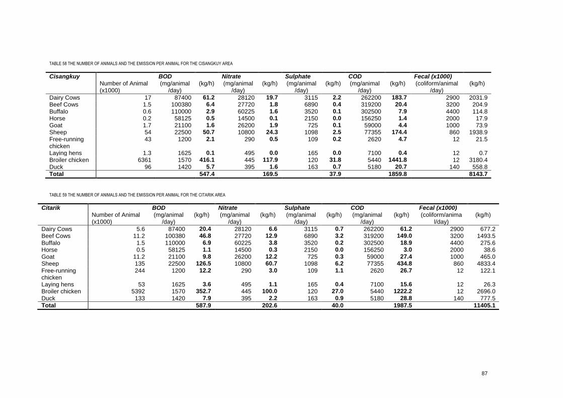
87
TABLE 58 THE NUMBER OF ANIMALS AND THE EMISSION PER ANIMAL FOR THE CISANGKUY AREA
Cisangkuy BOD Nitrate Sulphate COD Fecal (x1000) Number of Animal
(x1000) (mg/animal
/day) (kg/h) (mg/animal
/day) (kg/h) (mg/animal
/day) (kg/h) (mg/animal
/day) (kg/h) (coliform/animal
/day) (kg/h)
Dairy Cows 17 87400 61.2 28120 19.7 3115 2.2 262200 183.7 2900 2031.9 Beef Cows 1.5 100380 6.4 27720 1.8 6890 0.4 319200 20.4 3200 204.9 Buffalo 0.6 110000 2.9 60225 1.6 3520 0.1 302500 7.9 4400 114.8 Horse 0.2 58125 0.5 14500 0.1 2150 0.0 156250 1.4 2000 17.9 Goat 1.7 21100 1.6 26200 1.9 725 0.1 59000 4.4 1000 73.9 Sheep 54 22500 50.7 10800 24.3 1098 2.5 77355 174.4 860 1938.9 Free-running chicken
43 1200 2.1 290 0.5 109 0.2 2620 4.7 12 21.5
Laying hens 1.3 1625 0.1 495 0.0 165 0.0 7100 0.4 12 0.7 Broiler chicken 6361 1570 416.1 445 117.9 120 31.8 5440 1441.8 12 3180.4 Duck 96 1420 5.7 395 1.6 163 0.7 5180 20.7 140 558.8
Total 547.4 169.5 37.9 1859.8 8143.7
TABLE 59 THE NUMBER OF ANIMALS AND THE EMISSION PER ANIMAL FOR THE CITARIK AREA
Citarik BOD Nitrate Sulphate COD Fecal (x1000) Number of Animal
(x1000) (mg/animal
/day) (kg/h) (mg/animal
/day) (kg/h) (mg/animal
/day) (kg/h) (mg/animal
/day) (kg/h) (coliform/anima
l/day) (kg/h)
Dairy Cows 5.6 87400 20.4 28120 6.6 3115 0.7 262200 61.2 2900 677.2 Beef Cows 11.2 100380 46.8 27720 12.9 6890 3.2 319200 149.0 3200 1493.5 Buffalo 1.5 110000 6.9 60225 3.8 3520 0.2 302500 18.9 4400 275.6 Horse 0.5 58125 1.1 14500 0.3 2150 0.0 156250 3.0 2000 38.6 Goat 11.2 21100 9.8 26200 12.2 725 0.3 59000 27.4 1000 465.0 Sheep 135 22500 126.5 10800 60.7 1098 6.2 77355 434.8 860 4833.4 Free-running chicken
244 1200 12.2 290 3.0 109 1.1 2620 26.7 12 122.1
Laying hens 53 1625 3.6 495 1.1 165 0.4 7100 15.6 12 26.3 Broiler chicken 5392 1570 352.7 445 100.0 120 27.0 5440 1222.2 12 2696.0 Duck 133 1420 7.9 395 2.2 163 0.9 5180 28.8 140 777.5
Total 587.9 202.6 40.0 1987.5 11405.1
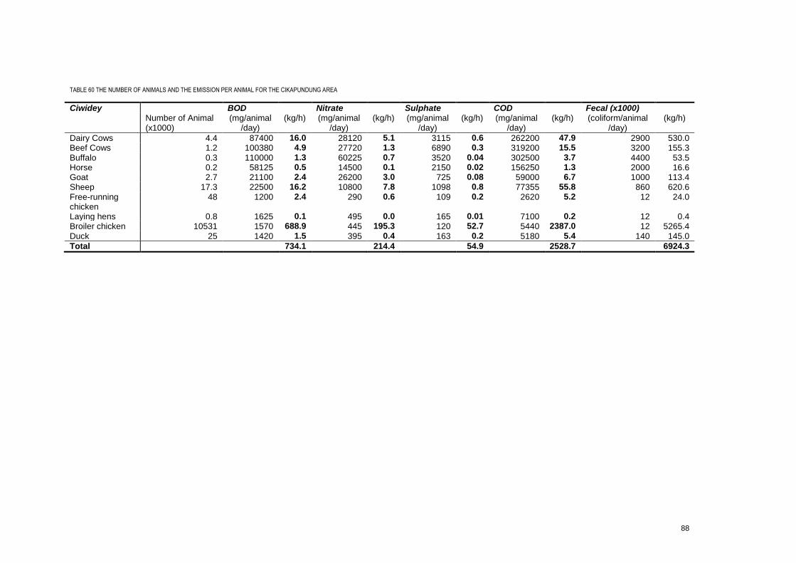
88
TABLE 60 THE NUMBER OF ANIMALS AND THE EMISSION PER ANIMAL FOR THE CIKAPUNDUNG AREA
Ciwidey BOD Nitrate Sulphate COD Fecal (x1000) Number of Animal
(x1000) (mg/animal
/day) (kg/h) (mg/animal
/day) (kg/h) (mg/animal
/day) (kg/h) (mg/animal
/day) (kg/h) (coliform/animal
/day) (kg/h)
Dairy Cows 4.4 87400 16.0 28120 5.1 3115 0.6 262200 47.9 2900 530.0 Beef Cows 1.2 100380 4.9 27720 1.3 6890 0.3 319200 15.5 3200 155.3 Buffalo 0.3 110000 1.3 60225 0.7 3520 0.04 302500 3.7 4400 53.5 Horse 0.2 58125 0.5 14500 0.1 2150 0.02 156250 1.3 2000 16.6 Goat 2.7 21100 2.4 26200 3.0 725 0.08 59000 6.7 1000 113.4 Sheep 17.3 22500 16.2 10800 7.8 1098 0.8 77355 55.8 860 620.6 Free-running chicken
48 1200 2.4 290 0.6 109 0.2 2620 5.2 12 24.0
Laying hens 0.8 1625 0.1 495 0.0 165 0.01 7100 0.2 12 0.4 Broiler chicken 10531 1570 688.9 445 195.3 120 52.7 5440 2387.0 12 5265.4 Duck 25 1420 1.5 395 0.4 163 0.2 5180 5.4 140 145.0
Total 734.1 214.4 54.9 2528.7 6924.3
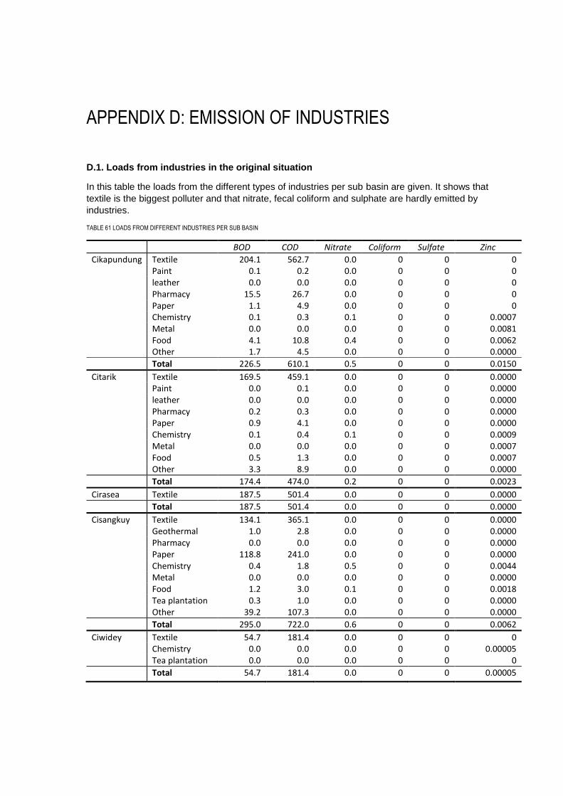
APPENDIX D: EMISSION OF INDUSTRIES
D.1. Loads from industries in the original situation
In this table the loads from the different types of industries per sub basin are given. It shows that
textile is the biggest polluter and that nitrate, fecal coliform and sulphate are hardly emitted by
industries.
TABLE 61 LOADS FROM DIFFERENT INDUSTRIES PER SUB BASIN
BOD COD Nitrate Coliform Sulfate Zinc
Cikapundung Textile 204.1 562.7 0.0 0 0 0 Paint 0.1 0.2 0.0 0 0 0 leather 0.0 0.0 0.0 0 0 0 Pharmacy 15.5 26.7 0.0 0 0 0 Paper 1.1 4.9 0.0 0 0 0 Chemistry 0.1 0.3 0.1 0 0 0.0007 Metal 0.0 0.0 0.0 0 0 0.0081 Food 4.1 10.8 0.4 0 0 0.0062 Other 1.7 4.5 0.0 0 0 0.0000
Total 226.5 610.1 0.5 0 0 0.0150
Citarik Textile 169.5 459.1 0.0 0 0 0.0000 Paint 0.0 0.1 0.0 0 0 0.0000 leather 0.0 0.0 0.0 0 0 0.0000 Pharmacy 0.2 0.3 0.0 0 0 0.0000 Paper 0.9 4.1 0.0 0 0 0.0000 Chemistry 0.1 0.4 0.1 0 0 0.0009 Metal 0.0 0.0 0.0 0 0 0.0007 Food 0.5 1.3 0.0 0 0 0.0007 Other 3.3 8.9 0.0 0 0 0.0000
Total 174.4 474.0 0.2 0 0 0.0023
Cirasea Textile 187.5 501.4 0.0 0 0 0.0000
Total 187.5 501.4 0.0 0 0 0.0000
Cisangkuy Textile 134.1 365.1 0.0 0 0 0.0000 Geothermal 1.0 2.8 0.0 0 0 0.0000 Pharmacy 0.0 0.0 0.0 0 0 0.0000 Paper 118.8 241.0 0.0 0 0 0.0000 Chemistry 0.4 1.8 0.5 0 0 0.0044 Metal 0.0 0.0 0.0 0 0 0.0000 Food 1.2 3.0 0.1 0 0 0.0018 Tea plantation 0.3 1.0 0.0 0 0 0.0000 Other 39.2 107.3 0.0 0 0 0.0000
Total 295.0 722.0 0.6 0 0 0.0062
Ciwidey Textile 54.7 181.4 0.0 0 0 0 Chemistry 0.0 0.0 0.0 0 0 0.00005 Tea plantation 0.0 0.0 0.0 0 0 0
Total 54.7 181.4 0.0 0 0 0.00005
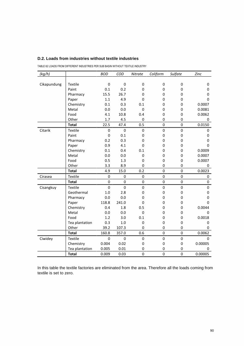
90
D.2. Loads from industries without textile industries
TABLE 62 LOADS FROM DIFFERENT INDUSTRIES PER SUB BASIN WITHOUT TEXTILE INDUSTRY
In this table the textile factories are eliminated from the area. Therefore all the loads coming from
textile is set to zero.
(kg/h) BOD COD Nitrate Coliform Sulfate Zinc
Cikapundung Textile 0 0 0 0 0 0 Paint 0.1 0.2 0 0 0 0 Pharmacy 15.5 26.7 0 0 0 0 Paper 1.1 4.9 0 0 0 0 Chemistry 0.1 0.3 0.1 0 0 0.0007 Metal 0.0 0.0 0 0 0 0.0081 Food 4.1 10.8 0.4 0 0 0.0062 Other 1.7 4.5 0 0 0 0
Total 22.5 47.4 0.5 0 0 0.0150
Citarik Textile 0 0 0 0 0 0 Paint 0 0.1 0 0 0 0 Pharmacy 0.2 0.3 0 0 0 0 Paper 0.9 4.1 0 0 0 0 Chemistry 0.1 0.4 0.1 0 0 0.0009 Metal 0.0 0.0 0 0 0 0.0007 Food 0.5 1.3 0 0 0 0.0007 Other 3.3 8.9 0 0 0 0
Total 4.9 15.0 0.2 0 0 0.0023
Cirasea Textile 0 0 0 0 0 0
Total 0 0 0 0 0 0
Cisangkuy Textile 0 0 0 0 0 0 Geothermal 1.0 2.8 0 0 0 0 Pharmacy 0.0 0.0 0 0 0 0 Paper 118.8 241.0 0 0 0 0 Chemistry 0.4 1.8 0.5 0 0 0.0044 Metal 0.0 0.0 0 0 0 0 Food 1.2 3.0 0.1 0 0 0.0018 Tea plantation 0.3 1.0 0 0 0 0 Other 39.2 107.3 0 0 0 0
Total 160.8 357.0 0.6 0 0 0.0062
Ciwidey Textile 0 0 0 0 0 0 Chemistry 0.004 0.02 0 0 0 0.00005 Tea plantation 0.005 0.01 0 0 0 0
Total 0.009 0.03 0 0 0 0.00005
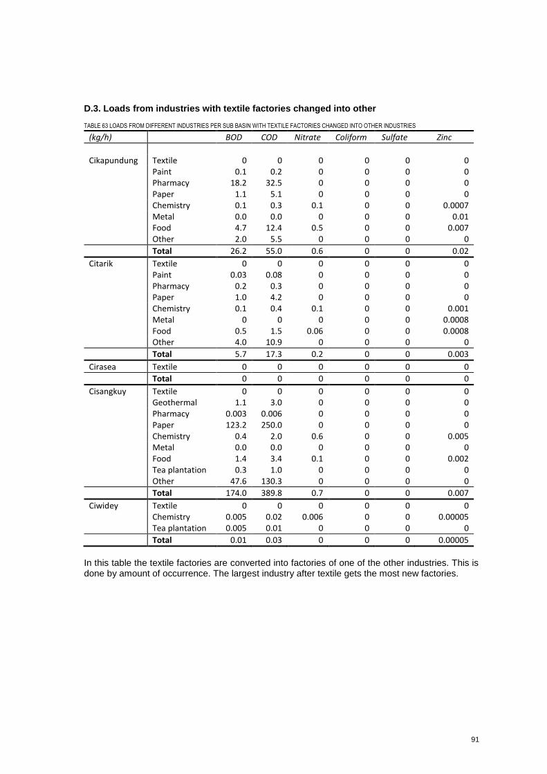
91
D.3. Loads from industries with textile factories changed into other
TABLE 63 LOADS FROM DIFFERENT INDUSTRIES PER SUB BASIN WITH TEXTILE FACTORIES CHANGED INTO OTHER INDUSTRIES
In this table the textile factories are converted into factories of one of the other industries. This is done by amount of occurrence. The largest industry after textile gets the most new factories.
(kg/h) BOD COD Nitrate Coliform Sulfate Zinc
Cikapundung Textile 0 0 0 0 0 0 Paint 0.1 0.2 0 0 0 0 Pharmacy 18.2 32.5 0 0 0 0 Paper 1.1 5.1 0 0 0 0 Chemistry 0.1 0.3 0.1 0 0 0.0007 Metal 0.0 0.0 0 0 0 0.01 Food 4.7 12.4 0.5 0 0 0.007 Other 2.0 5.5 0 0 0 0
Total 26.2 55.0 0.6 0 0 0.02
Citarik Textile 0 0 0 0 0 0 Paint 0.03 0.08 0 0 0 0 Pharmacy 0.2 0.3 0 0 0 0 Paper 1.0 4.2 0 0 0 0 Chemistry 0.1 0.4 0.1 0 0 0.001 Metal 0 0 0 0 0 0.0008 Food 0.5 1.5 0.06 0 0 0.0008 Other 4.0 10.9 0 0 0 0
Total 5.7 17.3 0.2 0 0 0.003
Cirasea Textile 0 0 0 0 0 0
Total 0 0 0 0 0 0
Cisangkuy Textile 0 0 0 0 0 0 Geothermal 1.1 3.0 0 0 0 0 Pharmacy 0.003 0.006 0 0 0 0 Paper 123.2 250.0 0 0 0 0 Chemistry 0.4 2.0 0.6 0 0 0.005 Metal 0.0 0.0 0 0 0 0 Food 1.4 3.4 0.1 0 0 0.002 Tea plantation 0.3 1.0 0 0 0 0 Other 47.6 130.3 0 0 0 0
Total 174.0 389.8 0.7 0 0 0.007
Ciwidey Textile 0 0 0 0 0 0 Chemistry 0.005 0.02 0.006 0 0 0.00005 Tea plantation 0.005 0.01 0 0 0 0
Total 0.01 0.03 0 0 0 0.00005
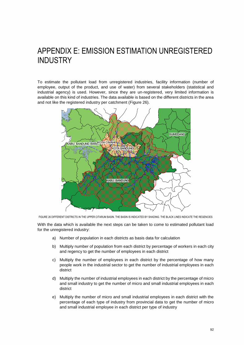
92
APPENDIX E: EMISSION ESTIMATION UNREGISTERED INDUSTRY
To estimate the pollutant load from unregistered industries, facility information (number of
employee, output of the product, and use of water) from several stakeholders (statistical and
industrial agency) is used. However, since they are un-registered, very limited information is
available on this kind of industries. The data available is based on the different districts in the area
and not like the registered industry per catchment (Figure 26).
FIGURE 26 DIFFERENT DISTRICTS IN THE UPPER CITARUM BASIN. THE BASIN IS INDICATED BY SHADING. THE BLACK LINES INDICATE THE REGENCIES
With the data which is available the next steps can be taken to come to estimated pollutant load
for the unregistered industry:
a) Number of population in each districts as basis data for calculation
b) Multiply number of population from each district by percentage of workers in each city
and regency to get the number of employees in each district
c) Multiply the number of employees in each district by the percentage of how many
people work in the industrial sector to get the number of industrial employees in each
district
d) Multiply the number of industrial employees in each district by the percentage of micro
and small industry to get the number of micro and small industrial employees in each
district
e) Multiply the number of micro and small industrial employees in each district with the
percentage of each type of industry from provincial data to get the number of micro
and small industrial employee in each district per type of industry
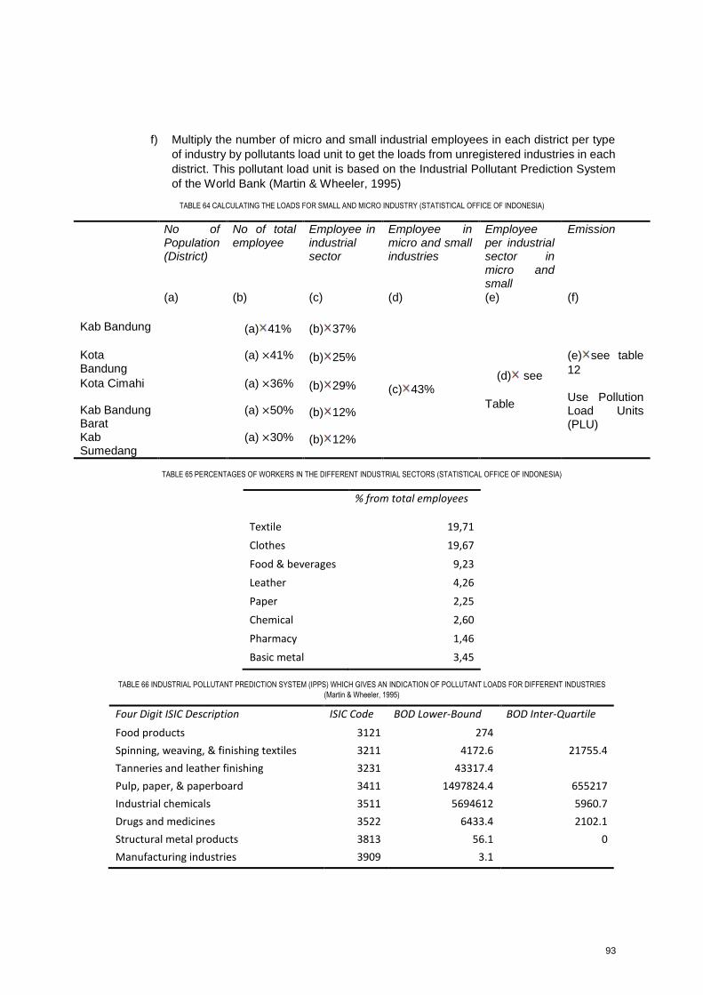
93
f) Multiply the number of micro and small industrial employees in each district per type
of industry by pollutants load unit to get the loads from unregistered industries in each
district. This pollutant load unit is based on the Industrial Pollutant Prediction System
of the World Bank (Martin & Wheeler, 1995)
TABLE 64 CALCULATING THE LOADS FOR SMALL AND MICRO INDUSTRY (STATISTICAL OFFICE OF INDONESIA)
No of Population (District)
No of total employee
Employee in industrial sector
Employee in micro and small industries
Employee per industrial sector in micro and small
Emission
(a) (b) (c) (d) (e) (f)
Kab Bandung (a) 41% (b) 37%
(c) 43% (d) see
Table
(e) see table
12 Use Pollution Load Units (PLU)
Kota Bandung
(a) ×41% (b) 25%
Kota Cimahi (a) ×36% (b) 29%
Kab Bandung Barat
(a) ×50% (b) 12%
Kab Sumedang
(a) ×30% (b) 12%
TABLE 65 PERCENTAGES OF WORKERS IN THE DIFFERENT INDUSTRIAL SECTORS (STATISTICAL OFFICE OF INDONESIA)
% from total employees
Textile 19,71
Clothes 19,67
Food & beverages 9,23
Leather 4,26
Paper 2,25
Chemical 2,60
Pharmacy 1,46
Basic metal 3,45
TABLE 66 INDUSTRIAL POLLUTANT PREDICTION SYSTEM (IPPS) WHICH GIVES AN INDICATION OF POLLUTANT LOADS FOR DIFFERENT INDUSTRIES
(Martin & Wheeler, 1995)
Four Digit ISIC Description ISIC Code BOD Lower-Bound BOD Inter-Quartile
Food products 3121 274
Spinning, weaving, & finishing textiles 3211 4172.6 21755.4
Tanneries and leather finishing 3231 43317.4
Pulp, paper, & paperboard 3411 1497824.4 655217
Industrial chemicals 3511 5694612 5960.7
Drugs and medicines 3522 6433.4 2102.1
Structural metal products 3813 56.1 0
Manufacturing industries 3909 3.1
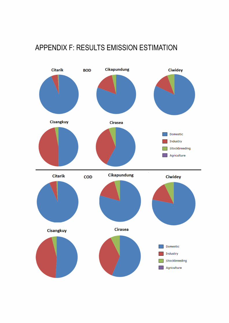
APPENDIX F: RESULTS EMISSION ESTIMATION