Embed Size (px)
Citation preview

Modeling Integrated Biomass Gasification Business Concepts Peter J. InceEdward M. (Ted) BilekMark A. Dietenberger
United StatesDepartment ofAgriculture
Forest Service
ForestProductsLaboratory
ResearchPaperFPL–RP–660
June 2011
Ince, Peter J.; Bilek, Edward M. (Ted); Dietenberger, Mark A. 2011. Modeling integrated biomass gasification business concepts. Research Paper FPL-RP-660. Madison, WI: U.S. Department of Agriculture, Forest Service, Forest Products Laboratory. 36 p.
A limited number of free copies of this publication are available to the public from the Forest Products Laboratory, One Gifford Pinchot Drive, Madison, WI 53726–2398. This publication is also available online at www.fpl.fs.fed.us. Laboratory publications are sent to hundreds of libraries in the United States and elsewhere.
The Forest Products Laboratory is maintained in cooperation with the University of Wisconsin.
The use of trade or firm names in this publication is for reader information and does not imply endorsement by the United States Department of Agriculture (USDA) of any product or service.
The USDA prohibits discrimination in all its programs and activities on the basis of race, color, national origin, age, disability, and where applicable, sex, marital status, familial status, parental status, religion, sexual orienta-tion, genetic information, political beliefs, reprisal, or because all or a part of an individual’s income is derived from any public assistance program. (Not all prohibited bases apply to all programs.) Persons with disabilities who require alternative means for communication of program informa-tion (Braille, large print, audiotape, etc.) should contact USDA’s TARGET Center at (202) 720–2600 (voice and TDD). To file a complaint of discrimi-nation, write to USDA, Director, Office of Civil Rights, 1400 Independence Avenue, S.W., Washington, D.C. 20250–9410, or call (800) 795–3272 (voice) or (202) 720–6382 (TDD). USDA is an equal opportunity provider and employer.
AbstractBiomass gasification is an approach to producing energy and/or biofuels that could be integrated into existing forest product production facilities, particularly at pulp mills. Existing process heat and power loads tend to favor integra-tion at existing pulp mills. This paper describes a generic modeling system for evaluating integrated biomass gasifica-tion business concepts over a range of production scales and process options, including process models and a discounted cash-flow model, all of which are contained in a Microsoft® (Redmond, Washington) Office Excel workbook (available from the authors). The process models encompass biomass preparation, gasification, heat recovery, and syngas cleanup, along with the options of converting syngas to biofuel feed-stocks via a Fischer–Tropsch gas-to-liquid (GTL) process, the use of syngas or GTL tail gas for process heat energy, and the option of added process energy equipment, includ-ing turbines and generators. The cash-flow model computes measures of financial performance for incremental invest-ment in gasification business concepts, including net present value and internal rate of return. We also describe stochastic simulation methods for financial risk assessment, and we present results of sensitivity analysis and stochastic simula-tion for investment in a biomass-to-liquid-fuel concept at an existing pulp mill, based on plausible but hypothetical process data and stochastic price projections. The results, as reinforced by the sensitivity analysis and risk assessment, suggest an investment may be attractive from a financial standpoint.
Keywords: Biofuels, biomass gasification, economic feasibility, forest biorefinery model
AcknowledgmentsThe authors gratefully acknowledge the advice and assis-tance of those who contributed expertise, information, and helpful suggestions as we developed the generic process model and prepared this report, including representatives of ThermoChem Recovery International, Inc. (TRI), Flambeau River Biofuels LLC, Emerging Fuels Technologies (EFT), and the U.S. Department of Energy National Renewable Energy Laboratory (NREL). We also gratefully acknowl-edge the contributions of research collaborators, including Professor Ross Swaney, University of Wisconsin–Madison, who contributed the prototypical process design and cost estimate for the Fischer–Tropsch component of the biorefin-ery concept (Appendix C), and Dr. John Zerbe (retired) of the Forest Products Laboratory who provided estimates of process parameters and costs for biomass drying equipment.
ContentsIntroduction .......................................................................... 1Integrated Biomass Gasification Concept ............................ 1Process Models and Parameters ........................................... 2 Base Case Model .............................................................. 3 Business Case Model ....................................................... 5 Biomass Procurement ...................................................... 5 Biomass Preparation and Drying ..................................... 6 Biomass Gasification ....................................................... 7 Syngas Heat Recovery and Cleanup .............................. 10 Gas-to-Liquid and Distillation ....................................... 11 Energy System Upgrades ............................................... 13Cash-Flow Model............................................................... 14 Annual Operating Costs and Revenue ........................... 15 Capital Costs .................................................................. 16 Taxes, Credits, and Incentives ........................................ 17 Economic Assumptions and Financing Options ............ 17 Incremental Cash Flows ................................................. 19 Measures of Performance and Sensitivity ...................... 20Risk Analysis and Stochastic Risk Assessment ................. 22Multivariate Stochastic Simulation .................................... 23Summary ............................................................................ 26References .......................................................................... 27Appendix A—Base Case Process Model Relationships ...................................................................... 28Appendix B—Business Case Process Model Relationships ...................................................................... 30Appendix C—GTL Plant Prototypical Design and Costs ................................................................................... 32 Fischer–Tropsch Component of the Forest Biorefinery Study: Prototypical Process Design and Cost Estimate .......................................................................... 32 Background and Description .......................................... 32 Design Basis and Assumptions ...................................... 32 Economics of the Design ............................................... 33 Analysis and Discussion of Design ................................ 34
Modeling Integrated Biomass Gasification Business ConceptsPeter J. Ince, Research ForesterEdward M. (Ted) Bilek, EconomistMark A. Dietenberger, Research General EngineerForest Products Laboratory, Madison, Wisconsin
IntroductionThe pulp and paper industry is a large consumer of energy as well as wood fiber raw materials; therefore, integrated biorefining and biomass energy systems are of interest within the industry. Thermochemical biorefining, based primarily on biomass gasification, is one of the leading plat-forms for new business concepts in integrated forest product biorefining (Connor 2007; Thorp et al. 2008a, 2008b). The economic feasibility of the integrated biomass gasification concept has also been explored in some previously pub-lished studies, such as an assessment of gasification-based biorefining at kraft pulp and paper mills in the United States developed at the Environmental Institute of Princeton Uni-versity (Larson et al. 2008, 2009; Agenda 2020 CTO Work-ing Group 2008a, 2008b).
Our research on generic modeling of the integrated biomass gasification business concept began in 2006, as the Potlatch Corporation (Spokane, Washington) was concluding an ex-ploratory assessment of the concept at a kraft pulp mill lo-cated in Warren, Arkansas. The gasification-based biorefin-ing concept looked promising in many ways, but researchers recognized that the likelihood of successfully establishing a new market for biomass gas-to-liquid products would improve if there were multiple entrants. As such, Potlatch and other industry representatives encouraged development of generic models of the concept so that other potential entrants could explore the same concept at other pulp mill locations. Our work on modeling the concept was largely a response to that need. Meanwhile, since 2006, the concept was also rigorously evaluated with the assistance of U.S. Department of Energy grants at two other U.S. pulp mill locations (at the Flambeau River Paper mill in Park Falls, Wisconsin, and at the NewPage paper mill in Wisconsin Rapids).
This report describes generic techniques we developed for modeling investments in integrated biomass gasification business concepts at existing forest product production facil-ities. We developed generic tools for preliminary analysis of the concept over a range of different production scales and process settings (e.g., potentially applicable to various mill locations). Our generic models are packaged in a Microsoft® Office (Redmond, Washington) Excel workbook file, which makes them portable and accessible to others. Interested
users may contact the authors of this paper to obtain a free copy. The conceptual analysis we present in this report is based on hypothetical data and is generally not nearly as rigorous as site-specific assessments that have been done at mill locations mentioned above. Those assessments were developed with additional engineering input and have pro-gressed to fairly advanced stages of analysis. Our generic models are designed for preliminary stages of analysis. If preliminary results look promising, much greater due dili-gence and more sophisticated engineering will be needed to support subsequent development and investment decisions.
Integrated Biomass Gasification ConceptThis report describes generic modeling of a business con-cept called integrated biomass gasification, which could include facilities for biomass preparation, biomass gasifica-tion, syngas cleanup, heat recovery, gas-to-liquid (Fischer–Tropsch (FT)) and related energy systems in the context of an existing wood pulp mill or other large forest products facility. The concept that we describe is similar to that de-scribed by Connor (2007), and also similar to the “Phase 1” biomass gasification concept as described in a recent article by the paper industry’s Agenda 2020 CTO Working Group (2008a). This report does not involve the concept of black liquor gasification (known as “Phase 2”), which is another biorefining concept that has been explored by others (Larson and others 2008, 2009).
As defined by the American Forest & Paper Association (AF&PA) Agenda 2020 CTO Working Group (2008a) the “Phase 1” concept specifically means the installation at a pulp mill of a biomass gasification plant to produce syngas. The syngas could be used to produce liquid transporta-tion fuels (e.g., diesel fuel) and other co-products (alkanes and paraffinic waxes), which would require installation of syngas cleanup, cooling and conditioning equipment, plus a Fischer–Tropsch gas-to-liquids (GTL) plant. The concept also involves production synergies with the pulp mill in the form of energy supplied by the gasification process, which may involve cogeneration of power and displacement of fossil fuels. For example, syngas or residual tail gas from the GTL plant can displace natural gas (used chiefly in the lime kiln of a kraft pulp mill), and can also be used as fuel
Research Paper FPL–RP–660
2
to generate steam and electric power. Also, according to the Agenda 2020 CTO Working Group (2008a), the “Phase 1” concept (biomass gasification) appears to be technically feasible within the capability of existing commercially available equipment and carries somewhat less risk than the Phase 2 concept (black liquor gasification).
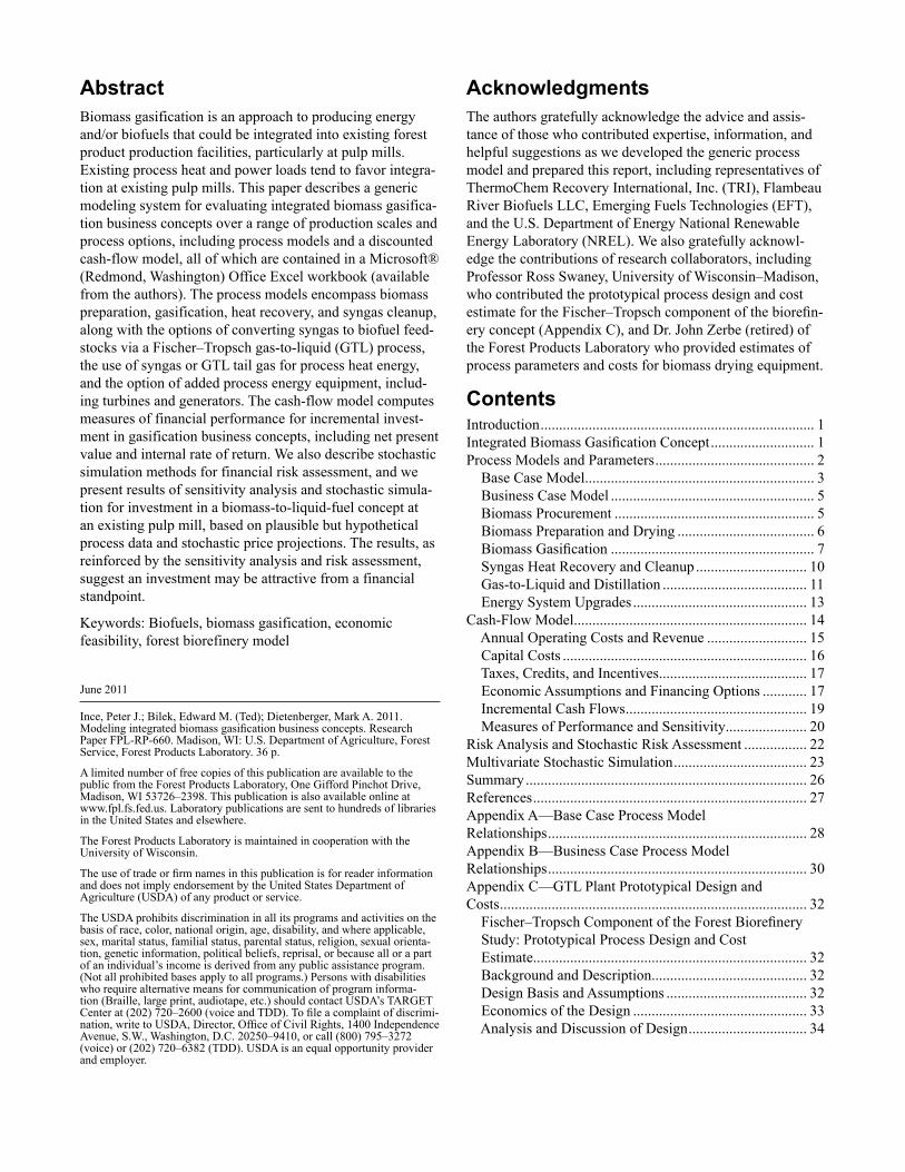
Figure 1 is a diagram of process elements that are included in the integrated biomass gasification concept described in this report. Pulp mills vary in design and energy require-ments, so optimal design of an integrated biomass gasifica-tion system would vary in terms of related pulp mill energy systems such as electrical generating facilities or auxiliary boilers. There is also the option of producing syngas only (e.g., producer gas as a fuel for displacement of natural gas), which would not require the GTL process nor as much syngas cleanup. That more limited option has been called “Phase 1: Option 1,” whereas biomass gasification coupled with the Fischer–Tropsch GTL process is called “Phase 1: Option 2” (Agenda 2020 CTO Working Group 2008a). Op-tion 2 is, of course, more complex and requires generally more capital investment than Option 1. Option 2 would also involve the marketing challenges and opportunities of introducing to an existing pulp mill a range of new products (Fischer–Tropsch biofuels and related co-products). The models that we describe in this report can be used to evalu-ate either “Option 1” or “Option 2” biomass gasification concepts.
Biomass could be purchased wood or bark or mill or agri-cultural residue. Biomass preparation equipment could con-sist of conventional chippers or hammermills and screens, followed by drying, as in a conventional rotary drum dryer. Various types of equipment are available for biomass gasifi-cation (or reforming) but choice of equipment can influence other process options. A wider range of gasification equip-ment is applicable if Option 1 is the sole objective—produc-tion of producer gas for combustion only (e.g., to displace natural gas). However, if Option 2 (GTL) is a current or future objective, then gasification equipment must be
capable of producing higher energy syngas to allow efficient conversion in the GTL process. Some biomass gasifiers can also generate hot flue gases that may be used to provide heat for biomass drying. In addition, with Option 2, syngas heat recovery and gas cleanup will be employed because the cat-alytic GTL process operates at lower gas temperatures, and impurities must be removed from syngas to avoid fouling of catalysts used in the GTL process.
Although not shown in Figure 1, integration of a new bio-mass gasification system to a pulp mill could also involve energy system upgrades, such as additional boiler capacity, electrical generating capacity, or steam handling capacity, along with possible modification of other existing pulp mill facilities such as wood handling or lime kiln operations. The process models that we developed allow for simulation of a number of alternative process arrangements, including Op-tion 1 or Option 2 arrangements mentioned previously, as well as different options in terms of energy system upgrades or combined heat and power production.
Process Models and ParametersThe process models consist of mathematical relationships that compute process input requirements, overall operating revenue, and overall operating costs for a specific forest product production facility both before and after introduc-tion of integrated biomass gasification. Computations are based on specific parameter values as determined by input data. All parameter relationships and input data are con-tained in the Excel workbook. Changing any input data will change parameter values and result in changing the estimat-ed operating revenue or costs and the projected economic performance of the production facility.
Two process models are in the Excel workbook: the “base case” model, and the “business case” model. The base case model describes operating revenue and costs at an existing forest product facility before introduction of biomass gasifi-cation. The business case model projects operating costs and revenue at the same facility after introduction of integrated
Figure 1. Process elements of biomass gasification concept with gas-to-liquid.
Modeling Integrated Biomass Gasification Business Concepts
3
biomass gasification technology. The difference in estimated operating revenue and costs between the two models pro-vides the incremental gain or loss in operating costs and rev-enue associated with the business concept (i.e., the biomass gasification concept). The models have some flexibility in specifying alternative scales of production and process configurations. The next section outlines the structure of the base case model and how input data and process parameters can be adjusted to simulate alternative mill configurations and scales of production at an existing forest product facili-ty. Subsequent sections outline process parameters, relation-ships, and input data for the business case model and each element of the integrated biomass gasification process.
Base Case ModelThe base case refers to an existing forest product produc-tion facility that is in operation prior to introduction of inte-grated biomass gasification technology. The base case model describes overall operating costs, revenue, and selected material and energy flows at the existing facility. The exist-ing facility may include an existing pulp mill or pulp and paper mill that may be operated in conjunction with other wood product mills (for example, a sawmill or plywood mill). Production of wood products (lumber or plywood) can generate wood or bark residue that may be used at the pulp mill. Our modeling framework is flexible in that it can represent a pulp mill alone, or a pulp and paper mill, which may be operated also in conjunction with one or more local wood product mills. In the hypothetical sample data that we included in this report, we represented a sawmill operating in conjunction with a pulp and paper mill.
The base case process model represents the primary mate-rial and energy flows likely to be directly affected by intro-duction of integrated biomass gasification. Thus, the base case process model includes pulp, paper, and wood product production volumes, costs, product revenue, timber procure-ment, and disposition of wood and bark residue, process steam, and energy flows, including electric power cogenera-tion, and process fuel inputs including natural gas for the lime kiln typically associated with a kraft pulp mill.
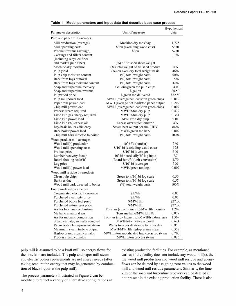
Table 1 lists all the model parameters that can be used to describe a base case process, which can be varied by scale or product output. The table includes hypothetical data val-ues as examples of model inputs. The hypothetical data in Table 1 do not pertain to any specific existing mill, but the scale of production and data values are thought to be typi-cal for a modern kraft pulp and paper mill facility, at 2008 price levels. A user can change input data for any parameter in Table 1 to represent a different mill situation or different market conditions.
The mass flow unit is short tons per day and the energy flow unit is megawatt hours per day for consistency with electric-ity and heating conventions. The engineer or scientific users can easily insert conversion of units in the spreadsheet to
suit their needs, whereas the typical user will benefit from consistency of units throughout the process model.
As shown in Table 1, we specified hypothetical input data for all parameters of the base case process (in this case a kraft pulp and paper mill operating in conjunction with saw-mill capacity). The parameters can be assigned different data values, and some can be assigned zero values when model-ing different types of production facilities. For example, if no wood product mill was operating in conjunction with the pulp and paper mill, then zero values would be assigned to all seven parameters under the subheading of “Wood product mill averages,” and all three parameters under the subheading of “Wood mill residue by-products.” This would effectively exclude wood product capacity from the model so that the model would represent a pulp and paper mill alone.
Alternative pulp mill technologies can also be represented by assigning alternative values to selected parameters. For example, if the pulp mill is not a kraft mill then it would typically not include a lime kiln, and thus zero values would be entered for the three parameters that pertain to the lime kiln (Lime Kiln Gas Energy Required, Lime Kiln Power Load, and Lime Kiln % Excess Air). Similarly, not all pulp mills include soap and turpentine recovery, and in that case zero values would be input for the two parameters that per-tain to soap and turpentine recovery (Soap & Turpentine Re-covery, and Soap & Turpentine Revenue). It is also possible to model a pulp mill only without a paper mill; for example, a mill that produces only market pulp. In that case, the Mill Production and Product Revenue parameters would be as-signed values that pertained to market pulp output, the Mill Operating Cost would pertain to the pulp mill only, and zero values would be entered for other parameters that pertained only to papermaking (such as Coatings & Fillers, and Paper Mill Power Load).
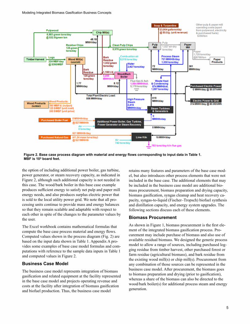
Figure 2 is the material and energy flow diagram for the base case process model, with computed values determined by data inputs in Table 1. The base case process diagram and computed material and energy flows are included in the Excel workbook. As illustrated in Figure 2, the paper mill, pulp mill, and other wood product mill(s) such as sawmill and chip mill(s) will typically have interrelated material and energy flows. For example, in the hypothetical case illus-trated in Figure 2, the paper mill consumes pulp that is produced at the pulp mill, which in turn consumes pulpwood chips obtained from a chip mill and also wood residue chips from a sawmill. The sawmill output and lumber recovery efficiency determine the quantities of pulpwood residue chip and bark residue outputs. The chip mill satisfies remaining needs for pulpwood chips and also produces bark residue. Bark residues are burned in a wood/bark boiler, which pro-vides high-pressure steam for cogeneration of electric power in steam turbines and generators, and lower pressure steam for pulp and paper mill process steam requirements. The
Research Paper FPL–RP–660
4
pulp mill is assumed to be a kraft mill, so energy flows for the lime kiln are included. The pulp and paper mill steam and electric power requirements are net energy needs (after taking account the energy that may be generated by combus-tion of black liquor at the pulp mill).
The process parameters illustrated in Figure 2 can be modified to reflect a variety of alternative configurations at
existing production facilities. For example, as mentioned earlier, if the facility does not include any wood mill(s), then the wood mill production and wood mill residue and energy flows can be deleted by assigning zero values to the wood mill and wood mill residue parameters. Similarly, the lime kiln or the soap and turpentine recovery can be deleted if not present in the existing production facility. There is also
Table 1—Model parameters and input data that describe base case process
Parameter description Unit of measure Hypothetical
data
Pulp and paper mill averages Mill production (average) Machine-dry tons/day 1,725 Mill operating costs $/ton (excluding wood cost) $350 Product revenue (average) $/ton $750 Coatings and fillers content (including recycled fiber and market pulp fiber) (%) of finished sheet weight
17%
Machine-dry moisture (%) total weight of finished product 4% Pulp yield (%) on oven dry total weight basis 46% Pulp chip moisture content (%) total weight basis 50% Bark from logs removal (%) total weight basis 15% Bark from logs moisture content (%) total weight basis 42% Soap and turpentine recovery Gallons/green ton pulp chips 4.0 Soap and turpentine revenue $/gallon $0.50 Pulpwood price $/green ton delivered $32.50 Pulp mill power load MWH (average net load)/ton green chips 0.012 Paper mill power load MWH (average net load)/ton paper output 0.209 Chip mill power load MWH (average net load)/ton green chips 0.007 Process steam required MWHth/ton dry pulp 0.472 Lime kiln gas energy required MWHth/ton dry pulp 0.341 Lime kiln power load MWH/ton dry pulp 0.01 Lime kiln (%) excess air Excess over stoichiometric 4% Dry-basis boiler efficiency Steam heat output per fuel HHV 84% Bark boiler power load MWH/green ton bark 0.007 Chip mill bark directed to boiler (%) total weight basis 100%
Wood product mill averages Wood mill(s) production 103 bf/d (lumber) 360 Wood mill operating costs $/103 bf (excluding wood cost) 125 Product price $/103 bf (average) 300 Lumber recovery factor 103 bf board tally/ft3 log input 7.7 Board foot log scale/ft3 Board foot/ft3 (unit conversion) 4.79 Log price $/103 bf (average) 390 Wood mill(s) power load MWH/green ton logs 0.007
Wood mill residue by-products Clean pulp chips Green tons/103 bf log scale 0.56 Bark residue Green tons/103 bf log scale 0.57 Wood mill bark directed to boiler (%) total weight basis 100%
Energy-related parameters Cogenerated electricity revenue $/kWh 0.05 Purchased electricity price $/kWh 0.07 Purchased boiler fuel price $/MWHth $27.00 Purchased natural gas price $/MWHth $27.00 Air for biomass combustion Tons air (stoichiometric)/MWHth biomass 1.208 Methane in natural gas Tons methane/MWHth NG 0.079 Air for methane combustion Tons air (stoichiometric)/MWHth natural gas 1.369 Steam enthalpy in water removal MWHth/ton water removal 0.624 Recoverable high-pressure steam Water tons per day/steam tons per day 0.950 Maximum steam turbine output MWH/MWHth high-pressure steam 0.357 High-pressure steam enthalpy MWHth/ton superheated high-pressure steam 0.700 Process steam enthalpy MWHth/ton process steam 0.825
Modeling Integrated Biomass Gasification Business Concepts
5
the option of including additional power boiler, gas turbine, power generator, or steam recovery capacity, as indicated in Figure 2, although such additional capacity is not needed in this case. The wood/bark boiler in this base case example produces sufficient energy to satisfy net pulp and paper mill energy needs, and also produces surplus electric power that is sold to the local utility power grid. We note that all pro-cessing units continue to provide mass and energy balances so that they remain scalable and adaptable with respect to each other in spite of the changes to the parameter values by the user.
The Excel workbook contains mathematical formulas that compute the base case process material and energy flows. Computed values shown in the process diagram (Fig. 2) are based on the input data shown in Table 1. Appendix A pro-vides some examples of base case model formulas and com-putations with reference to the sample data inputs in Table 1 and computed values in Figure 2.
Business Case ModelThe business case model represents integration of biomass gasification and related equipment at the facility represented in the base case model and projects operating revenue and costs at the facility after integration of biomass gasification and biofuel production. Thus, the business case model
retains many features and parameters of the base case mod-el, but also introduces other process elements that were not included in the base case. The additional elements that may be included in the business case model are additional bio-mass procurement, biomass preparation and drying capacity, biomass gasification, syngas cleanup and heat recovery ca-pacity, syngas-to-liquid (Fischer–Tropsch) biofuel synthesis and distillation capacity, and energy system upgrades. The following sections discuss each of these elements.
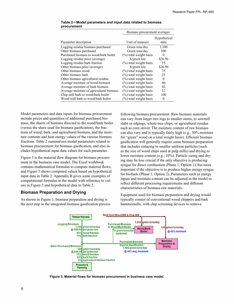
Biomass ProcurementAs shown in Figure 1, biomass procurement is the first ele-ment of the integrated biomass gasification process. Pro-curement may include purchase of biomass and also use of available residual biomass. We designed the generic process model to allow a range of sources, including purchased log-ging residue from timber harvest, other purchased forest or farm residue (agricultural biomass), and bark residue from the existing wood mill(s) or chip mill(s). Procurement from any combination of those sources can be represented in the business case model. After procurement, the biomass goes to biomass preparation and drying (prior to gasification), whereas a share of the biomass can also be directed to the wood/bark boiler(s) for additional process steam and energy generation.
Figure 2. Base case process diagram with material and energy flows corresponding to input data in Table 1. MBF is 103 board feet.
Research Paper FPL–RP–660
6
Model parameters and data inputs for biomass procurement include prices and quantities of additional purchased bio-mass, the shares of biomass directed to the wood/bark boiler (versus the share used for biomass gasification), the frac-tions of wood, bark, and agricultural biomass, and the mois-ture contents and heat energy values of the various biomass fractions. Table 2 summarizes model parameters related to biomass procurement for biomass gasification, and also in-cludes hypothetical input data values for each parameter.
Figure 3 is the material flow diagram for biomass procure-ment in the business case model. The Excel workbook contains mathematical formulas to compute material flows, and Figure 3 shows computed values based on hypothetical input data in Table 2. Appendix B gives some examples of computational formulas in the model with reference to val-ues in Figure 3 and hypothetical data in Table 2.
Biomass Preparation and DryingAs shown in Figure 1, biomass preparation and drying is the next step in the integrated biomass gasification process
following biomass procurement. Raw biomass materials can vary from larger tree logs to smaller stems, to sawmill slabs or edgings, whole-tree chips, or agricultural residue such as corn stover. The moisture content of raw biomass can also vary and is typically fairly high (e.g., 50% moisture for “green” wood on a total weight basis). Efficient biomass gasification will generally require some biomass preparation that includes reducing to smaller uniform particles (such as the size of wood chips used at pulp mills) and drying to lower moisture content (e.g., 10%). Particle sizing and dry-ing may be less crucial if the only objective is producing syngas for direct combustion (Phase 1, Option 1), but more important if the objective is to produce higher energy syngas for biofuels (Phase 1, Option 2). Parameters such as energy inputs and moisture content can be adjusted in the model to reflect different processing requirements and different characteristics of biomass raw materials.
Equipment used for biomass preparation and drying would typically consist of conventional wood chippers and bark hammermills, with chip screening devices to remove
Table 2—Model parameters and input data related to biomass procurement
Biomass procurement averages
Parameter description Unit of measure Hypothetical
dataLogging residue biomass purchased Green tons/day 1,100 Other biomass purchased Green tons/day 500 Purchased biomass to wood/bark boiler (%) total weight basis 0 Logging residue price (average) $/green ton $26.50 Logging residue bark fraction (%) total weight basis 15 Other biomass price (average) $/green ton $26.50 Other biomass wood (%) total weight basis 75 Other biomass bark (%) total weight basis 25 Other biomass agricultural residue (%) total weight basis 0 Average moisture of wood biomass (%) total weight basis 40 Average moisture of bark biomass (%) total weight basis 42 Average moisture of agricultural biomass (%) total weight basis 12 Chip mill bark to wood/bark boiler (%) total weight basis 100 Wood mill bark to wood/bark boiler (%) total weight basis 0
Figure 3. Material flows for biomass procurement in business case model.
Modeling Integrated Biomass Gasification Business Concepts
7
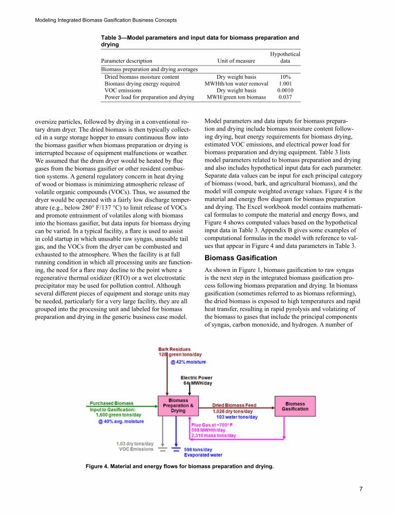
oversize particles, followed by drying in a conventional ro-tary drum dryer. The dried biomass is then typically collect-ed in a surge storage hopper to ensure continuous flow into the biomass gasifier when biomass preparation or drying is interrupted because of equipment malfunctions or weather. We assumed that the drum dryer would be heated by flue gases from the biomass gasifier or other resident combus-tion systems. A general regulatory concern in heat drying of wood or biomass is minimizing atmospheric release of volatile organic compounds (VOCs). Thus, we assumed the dryer would be operated with a fairly low discharge temper-ature (e.g., below 280° F/137 °C) to limit release of VOCs and promote entrainment of volatiles along with biomass into the biomass gasifier, but data inputs for biomass drying can be varied. In a typical facility, a flare is used to assist in cold startup in which unusable raw syngas, unusable tail gas, and the VOCs from the dryer can be combusted and exhausted to the atmosphere. When the facility is at full running condition in which all processing units are function-ing, the need for a flare may decline to the point where a regenerative thermal oxidizer (RTO) or a wet electrostatic precipitator may be used for pollution control. Although several different pieces of equipment and storage units may be needed, particularly for a very large facility, they are all grouped into the processing unit and labeled for biomass preparation and drying in the generic business case model.
Model parameters and data inputs for biomass prepara-tion and drying include biomass moisture content follow-ing drying, heat energy requirements for biomass drying, estimated VOC emissions, and electrical power load for biomass preparation and drying equipment. Table 3 lists model parameters related to biomass preparation and drying and also includes hypothetical input data for each parameter. Separate data values can be input for each principal category of biomass (wood, bark, and agricultural biomass), and the model will compute weighted average values. Figure 4 is the material and energy flow diagram for biomass preparation and drying. The Excel workbook model contains mathemati-cal formulas to compute the material and energy flows, and Figure 4 shows computed values based on the hypothetical input data in Table 3. Appendix B gives some examples of computational formulas in the model with reference to val-ues that appear in Figure 4 and data parameters in Table 3.
Biomass GasificationAs shown in Figure 1, biomass gasification to raw syngas is the next step in the integrated biomass gasification pro-cess following biomass preparation and drying. In biomass gasification (sometimes referred to as biomass reforming), the dried biomass is exposed to high temperatures and rapid heat transfer, resulting in rapid pyrolysis and volatizing of the biomass to gases that include the principal components of syngas, carbon monoxide, and hydrogen. A number of
Table 3—Model parameters and input data for biomass preparation and drying
Parameter description Unit of measure Hypothetical
dataBiomass preparation and drying averages
Dried biomass moisture content Dry weight basis 10% Biomass drying energy required MWHth/ton water removal 1.001 VOC emissions Dry weight basis 0.0010 Power load for preparation and drying MWH/green ton biomass 0.037
Figure 4. Material and energy flows for biomass preparation and drying.
Research Paper FPL–RP–660
8
different gasification technologies are available, ranging from technologies that admit air in the process to technolo-gies that mostly exclude air (such as steam reforming). Technologies that admit significant amounts of air may have lower costs but may also yield lower energy syngas because inert nitrogen is introduced by the air and because carbon dioxide is formed from reaction of carbon with oxygen in the air. Lower energy syngas may be acceptable for direct combustion (Phase 1, Option 1), but may not be suitable for efficient conversion of syngas to biofuels or chemicals via the Fischer–Tropsch process (Phase 1, Option 2). Thus the choice of gasifier technology may determine or constrain the options for syngas use.
Steam reforming is an example of biomass gasification technology that has potential to produce high energy syn-gas. In steam reforming, the dried biomass is exposed to superheated steam, while admission of air into the process is minimized (for example, biomass can be fed into a steam reformer with a plug screw that minimizes entrained air). As described by Connor (2007), the superheated steam (H2O) has an endothermic reaction with the carbon in the biomass, consuming heat from an external fuel source and producing hydrogen (H2) and carbon monoxide (CO), principal ingre-dients of synthesis gas or syngas. This reaction of superheat-ed steam with carbon is called steam reforming:
H2O + C + Heat → H2 + CO (1)
Likewise, some measure of pure oxygen (O2) can be used in oxygen reforming of carbon particles and char (or known as carbon trim):
O2 + 2C → 2CO + Heat (2)
O2 + 2CO → 2CO2 + Heat (3)
The water-gas shift reaction also occurs simultaneously with the steam and oxygen reforming reaction to yield additional hydrogen and carbon dioxide, also known as the water-gas shift reaction:
H2O + CO → H2 + CO2 + Heat (4)
Other intermediate reactions also occur, such as the for-mations of methane from carbon and hydrogen, carbon monoxide from carbon and carbon dioxide, hydrogen and carbon monoxide from methane with water vapor or carbon dioxide, and several other reactions. Most of these reac-tions are reversible, depending on reactant concentrations, temperature, and directions of energy flows. At the highest temperatures only the simplest gases are left, making the water gas shift the dominating reaction. In the end, steam, pure oxygen, biomass, and energy inputs can be modulated to yield a 2:1 molar ratio of hydrogen and carbon monoxide in syngas, which is ideal for the Fischer–Tropsch reaction. After the moisture and trace gas removals, syngas composi-tions may be obtained at molar percentages that are typical for biomass, such as 44.6% H2, 22.3% CO, 26.4% CO2, 4.5% CH4, 1.0% C2H4, and 1.2% N2.
Some steam-based gasifiers may be designed for the sim-pler, but less efficient and costlier, staging of these reactions into separate reaction vessels to obtain the targeted molar ratio of hydrogen and carbon monoxide. It is likely that varying levels of steam, carbon dioxide, nitrogen, and trace gases exist among these gasifiers even if their molar ratio of hydrogen and carbon monoxide is 2:1. The complexities and variations among the gasifiers and reformers lead us to identify basic parameters consistent with other processing units in the generic business case model without necessarily involving detailed engineering analysis of gasification reac-tions or revealing proprietary data.
Table 4—Model parameters and input data related to biomass gasification Hypothetical data
Parameter description and unit of measure Wood Bark Agricultural
residue Average Feedstock higher heating value (HHV) 4.707 5.227 3.894 4.829
(MWHth/dry ton biomass feed) Gasification thermal energy required 1.096 1.096 1.594 1.096
(MWHth/dry ton biomass feed) Reforming steam energy required 0.432 0.541 0.410 0.458
(MWHth/dry ton biomass) Energy content of gasifier producer gas (or raw syngas) 2.606 2.606 2.606 2.606
(MWHth/ton producer gas) Flue gas recoverable energy 0.490 0.909 0.797 0.588
(MWHth/dry ton biomass) Ash and char residue 0.031 0.026 0.159 0.030
(tons/dry ton biomass) Power load 0.131 0.131 0.131 0.131
(MWH/dry ton biomass) Oxygen feed for char gasification 0.237 0.245 0.186 0.239
(Tons/ton of dry biomass) Excess air in reformer fuel combustion 20
(% excess over stoichiometric requirement)
Modeling Integrated Biomass Gasification Business Concepts
9
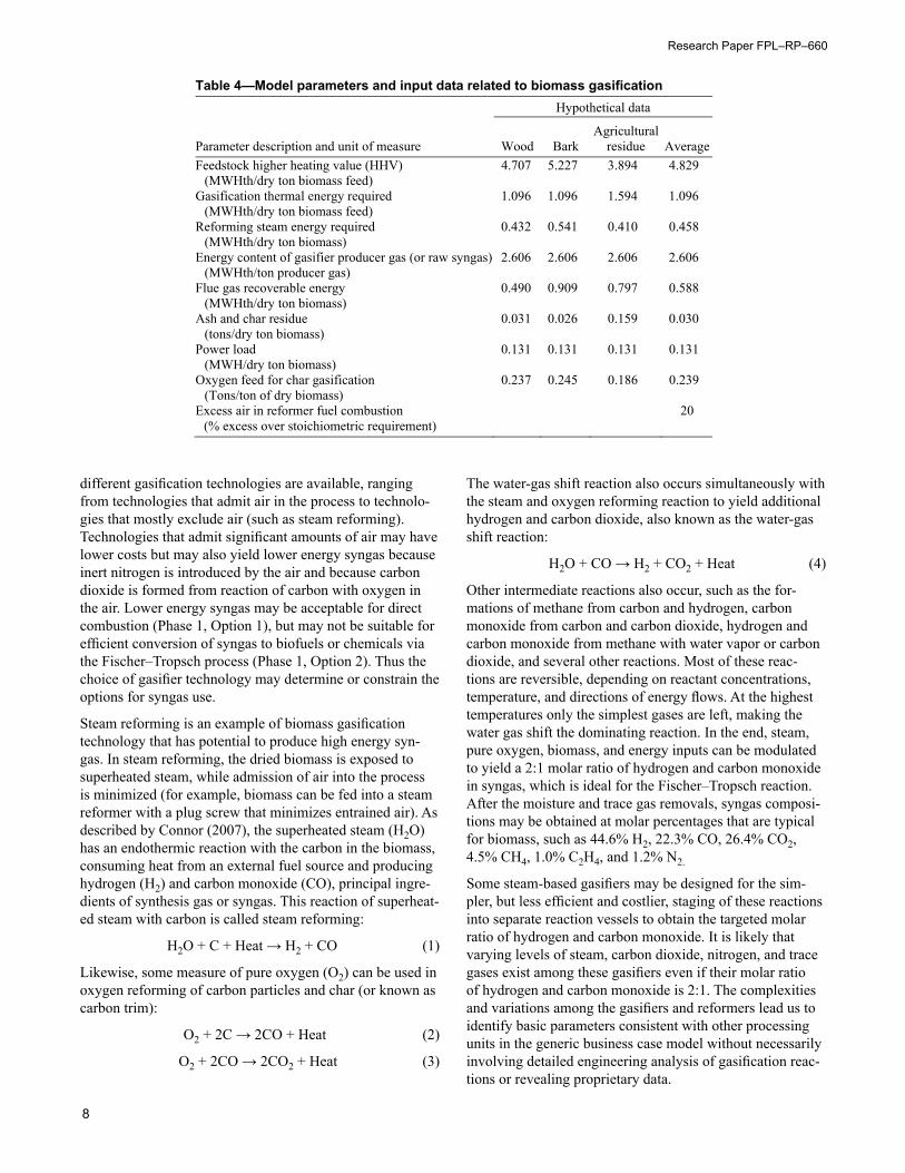
Regardless of technology, biomass gasification in general involves use of thermal energy to gasify biomass and reform it into syngas (carbon monoxide and hydrogen) plus other gases. Model parameters for biomass gasification include the combustion higher heating values of the dried biomass feedstocks, thermal energy required for biomass gasifica-tion, steam energy associated with the low-pressure steam mass required for steam reforming, energy content of pro-ducer gas or raw syngas, recoverable energy in gasifier flue gases, yield of ash and char residue, combustion heating value of char and ash residue, power load to operate gasifier and auxiliary equipment such as oxygen generators, oxygen needed for char gasification, and excess air in combustion of reformer fuel (tail gas or natural gas). Table 4 summarizes the model parameters related to biomass gasification and provides hypothetical data values for each parameter.
The hypothetical data in Table 4 are generalized conceptual estimates for steam-based gasification and are not consid-ered empirical data. In the end, experimental techniques and operational experience are the only way to obtain precise values for these parameters. Equipment vendors may also help provide data estimates. Some wood and bark heating value data can also be found in reference publications, such as Ince 1979, in which Table 1 provides higher heating val-ues for some wood and bark species that were reported in other publications.
The model computes “average” data values (last column of Table 4) as weighted averages based on input data for wood, bark, and agricultural residue, weighted by tonnage shares of each in the total biomass feedstock. Thus, if a particular category of biomass is not used (e.g., agricultural biomass is not used in this hypothetical case as shown earlier in Table 2), then its parameter values will not be factored into the averages (hence “average” values in Table 4 in this case are weighted averages for wood and bark only, not agricultural residue). Any input value can be changed, but as indicated in
the hypothetical data in Table 4, some typical characteristics of wood, bark, and agricultural residue must be considered in making adjustments to input data. For example, wood and bark typically have higher combustion heating values but lower ash content than agricultural residue. Different feedstock characteristics also influence gasification thermal energy requirements, recoverable flue gas energy, heating value of ash char, and oxygen feed for char gasification and oxidation trimming of raw syngas. As a result, the biomass gasification unit has become the most complex model fea-ture with the most parameters, and we expect that these parameters will be determined independently via empirical data or through detailed engineering analysis.
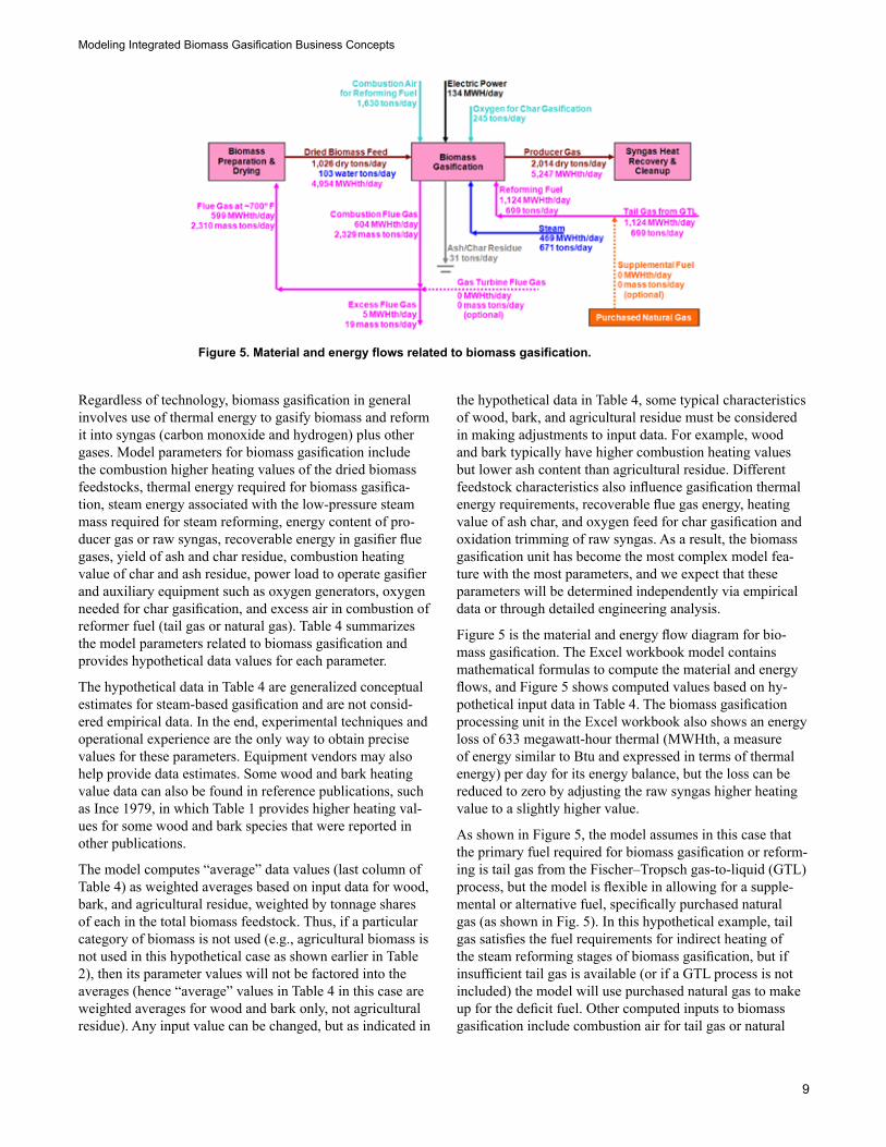
Figure 5 is the material and energy flow diagram for bio-mass gasification. The Excel workbook model contains mathematical formulas to compute the material and energy flows, and Figure 5 shows computed values based on hy-pothetical input data in Table 4. The biomass gasification processing unit in the Excel workbook also shows an energy loss of 633 megawatt-hour thermal (MWHth, a measure of energy similar to Btu and expressed in terms of thermal energy) per day for its energy balance, but the loss can be reduced to zero by adjusting the raw syngas higher heating value to a slightly higher value.
As shown in Figure 5, the model assumes in this case that the primary fuel required for biomass gasification or reform-ing is tail gas from the Fischer–Tropsch gas-to-liquid (GTL) process, but the model is flexible in allowing for a supple-mental or alternative fuel, specifically purchased natural gas (as shown in Fig. 5). In this hypothetical example, tail gas satisfies the fuel requirements for indirect heating of the steam reforming stages of biomass gasification, but if insufficient tail gas is available (or if a GTL process is not included) the model will use purchased natural gas to make up for the deficit fuel. Other computed inputs to biomass gasification include combustion air for tail gas or natural
Figure 5. Material and energy flows related to biomass gasification.
Research Paper FPL–RP–660
10
gas, electric power for gasifier equipment, oxygen for char gasification and any syngas oxidation trimming, and steam input. The model assumes that flue gas from combustion of tail gas or natural gas is used for biomass drying, but that may be supplemented or replaced by flue gas from a gas tur-bine (from a power boiler) as an optional arrangement.
To reconfigure the steam-based gasification to just an air-starved gasifier with the intent to produce low energy gas for heat and power applications, the parameters for indirect combustion heating can be set to zero (thereby eliminating this cost component), whereas the oxygen mass parameter and its heating value can be adjusted for partial combustion of raw syngas with air. Considerable empirical data should be available due to many installations of the air-starved gasifiers.
Syngas Heat Recovery and CleanupAs shown in Figure 1, syngas heat recovery and cleanup is the next step in the integrated biomass gasification process following biomass gasification. Heat recovery and syngas cleanup will be employed if the objective is to produce bio-fuels or chemicals via the Fischer–Tropsch process (Phase 1, Option 2), because the catalytic Fischer–Tropsch reaction occurs optimally at much lower temperatures and higher pressures than biomass gasification, and impurities such as tars and sulfur will foul the catalysts unless they are sub-stantially eliminated.
An effective typical sequence of syngas cleanup and heat recovery could involve multiple stages, including particu-late removal, heat recovery, removal of trace gases, and gas filtration. A series of cyclones and a venturi scrubber could be used to remove particulates, which would then be elimi-nated in the carbon trim unit or the gasifier, or would be flared. Heat recovery with a heat steam recovery generator (HSRG) unit may reduce syngas temperatures to the point where tar is condensed, which may also be eliminated in the carbon trim unit or the gasifier, or would be flared. In some syngas cleanup schemes, the tar is cracked or reformed be-fore the heat recovery to reduce or avoid tar condensation. The syngas may go through another heat recovery with an
HSRG unit to condense the syngas steam, with the resulting effluent cleaned and disposed of. Trace gas removal may go through various steps, including a hydrogen sulfide scrub-ber at atmospheric pressure, and then pressurization for efficient scrubbing stages of ammonia, H2S, and COS, and zinc polishing and filtering of micron-sized particles to very low concentration levels (e.g., less than one part per million) as may be needed before direct insertion into the Fischer–Tropsch catalytic reactor unit (to avoid reduced efficiency or fouling of catalysts). Other cleaning and heat recovery schemes are possible, but are not necessary to detail here, as multiple equipment arrangements are generally implied and grouped into the heat recovery and cleanup stage of the model.
If the objective is only to produce syngas clean enough and suitable for direct combustion, the initial removal of particu-lates, tar, steam, and much of H2S can be done with lower cost technology at atmospheric pressure, and in that case may not require the further pressurized cleaning needed in the Fischer–Tropsch reactor unit. So, if the only objective is to use the syngas for direct combustion (Phase 1, Option 1), then syngas heat recovery or cleanup requirements may be reduced or eliminated. The model is flexible in that pa-rameters related to syngas heat recovery and cleanup can be modified (or eliminated) to represent varying process objec-tives and requirements.
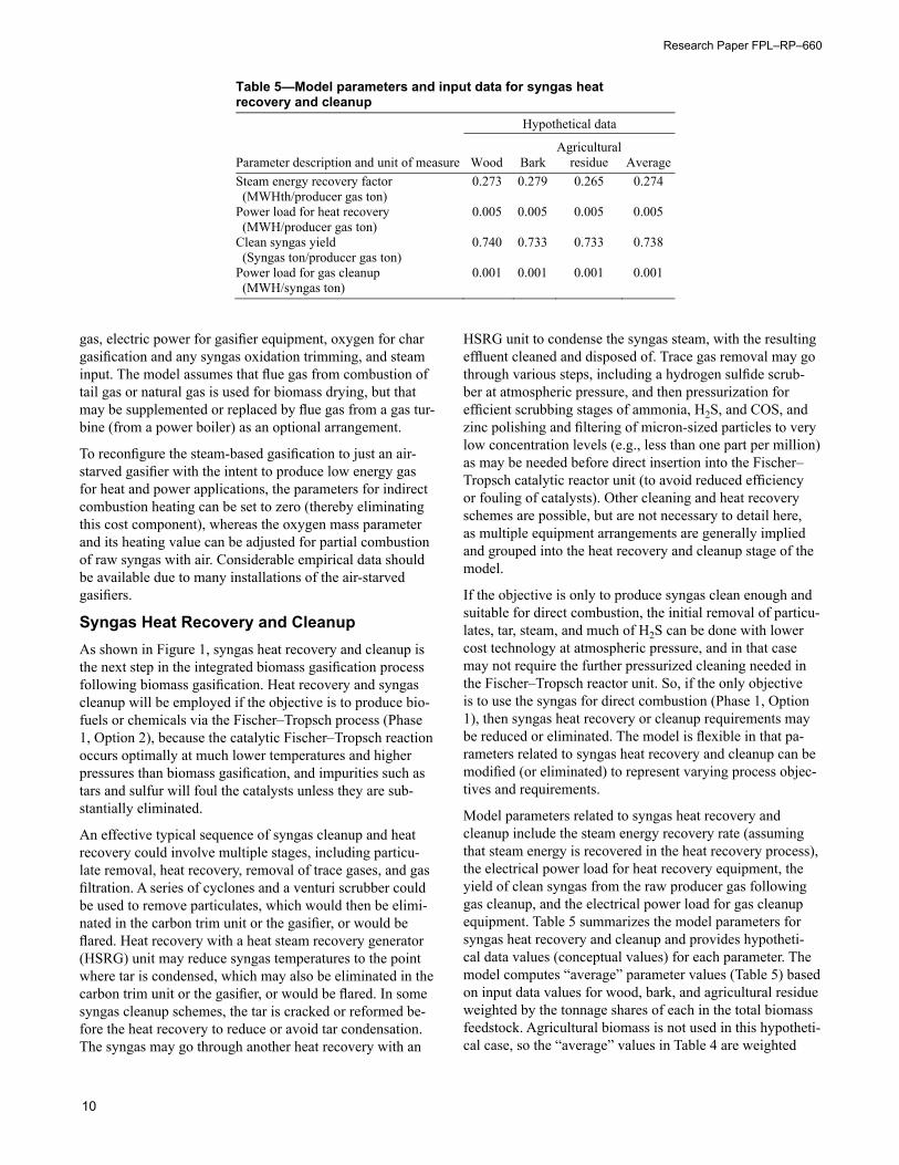
Model parameters related to syngas heat recovery and cleanup include the steam energy recovery rate (assuming that steam energy is recovered in the heat recovery process), the electrical power load for heat recovery equipment, the yield of clean syngas from the raw producer gas following gas cleanup, and the electrical power load for gas cleanup equipment. Table 5 summarizes the model parameters for syngas heat recovery and cleanup and provides hypotheti-cal data values (conceptual values) for each parameter. The model computes “average” parameter values (Table 5) based on input data values for wood, bark, and agricultural residue weighted by the tonnage shares of each in the total biomass feedstock. Agricultural biomass is not used in this hypotheti-cal case, so the “average” values in Table 4 are weighted
Table 5—Model parameters and input data for syngas heat recovery and cleanup
Hypothetical data
Parameter description and unit of measure Wood Bark Agricultural
residue Average Steam energy recovery factor 0.273 0.279 0.265 0.274 (MWHth/producer gas ton)
Power load for heat recovery 0.005 0.005 0.005 0.005 (MWH/producer gas ton)
Clean syngas yield 0.740 0.733 0.733 0.738 (Syngas ton/producer gas ton)
Power load for gas cleanup 0.001 0.001 0.001 0.001 (MWH/syngas ton)
Modeling Integrated Biomass Gasification Business Concepts
11
averages for wood and bark only and not the agricultural residue.
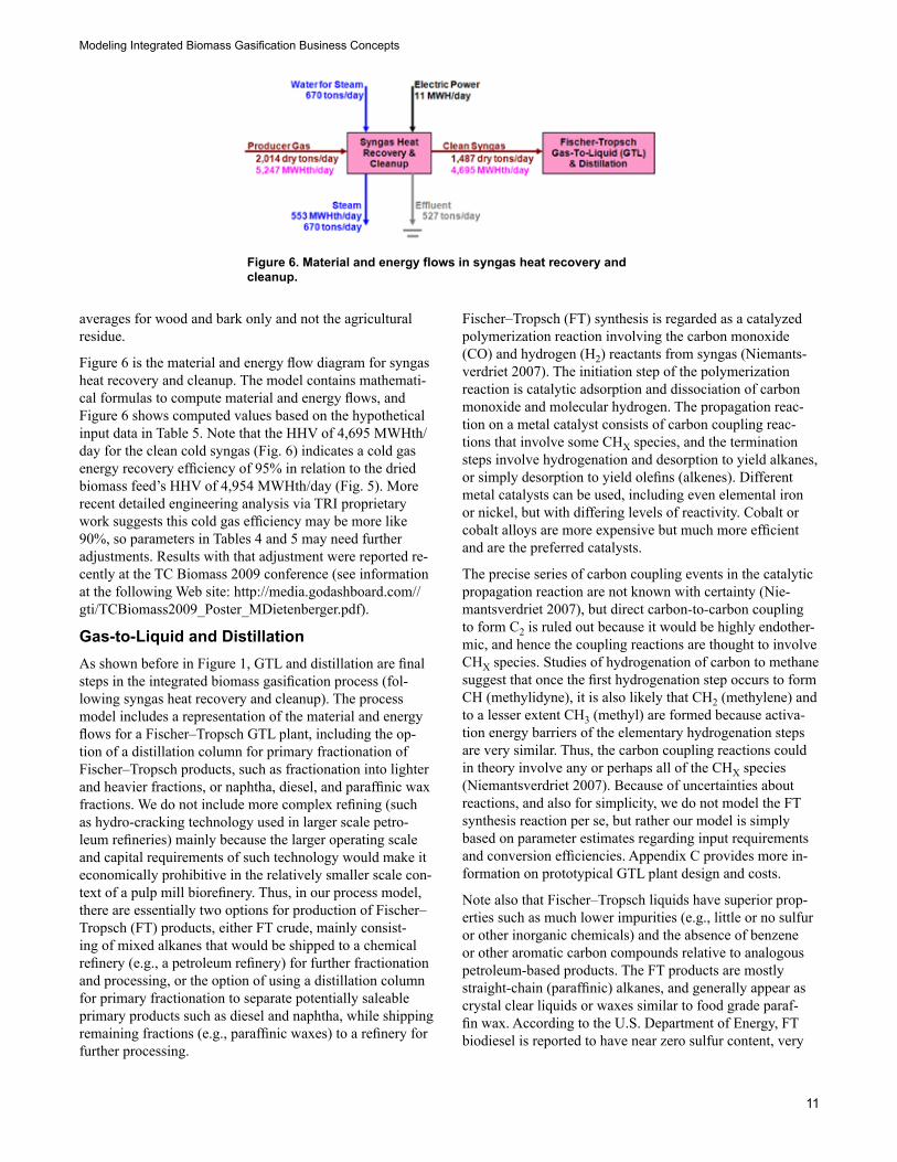
Figure 6 is the material and energy flow diagram for syngas heat recovery and cleanup. The model contains mathemati-cal formulas to compute material and energy flows, and Figure 6 shows computed values based on the hypothetical input data in Table 5. Note that the HHV of 4,695 MWHth/day for the clean cold syngas (Fig. 6) indicates a cold gas energy recovery efficiency of 95% in relation to the dried biomass feed’s HHV of 4,954 MWHth/day (Fig. 5). More recent detailed engineering analysis via TRI proprietary work suggests this cold gas efficiency may be more like 90%, so parameters in Tables 4 and 5 may need further adjustments. Results with that adjustment were reported re-cently at the TC Biomass 2009 conference (see information at the following Web site: http://media.godashboard.com//gti/TCBiomass2009_Poster_MDietenberger.pdf).
Gas-to-Liquid and DistillationAs shown before in Figure 1, GTL and distillation are final steps in the integrated biomass gasification process (fol-lowing syngas heat recovery and cleanup). The process model includes a representation of the material and energy flows for a Fischer–Tropsch GTL plant, including the op-tion of a distillation column for primary fractionation of Fischer–Tropsch products, such as fractionation into lighter and heavier fractions, or naphtha, diesel, and paraffinic wax fractions. We do not include more complex refining (such as hydro-cracking technology used in larger scale petro-leum refineries) mainly because the larger operating scale and capital requirements of such technology would make it economically prohibitive in the relatively smaller scale con-text of a pulp mill biorefinery. Thus, in our process model, there are essentially two options for production of Fischer–Tropsch (FT) products, either FT crude, mainly consist-ing of mixed alkanes that would be shipped to a chemical refinery (e.g., a petroleum refinery) for further fractionation and processing, or the option of using a distillation column for primary fractionation to separate potentially saleable primary products such as diesel and naphtha, while shipping remaining fractions (e.g., paraffinic waxes) to a refinery for further processing.
Fischer–Tropsch (FT) synthesis is regarded as a catalyzed polymerization reaction involving the carbon monoxide (CO) and hydrogen (H2) reactants from syngas (Niemants-verdriet 2007). The initiation step of the polymerization reaction is catalytic adsorption and dissociation of carbon monoxide and molecular hydrogen. The propagation reac-tion on a metal catalyst consists of carbon coupling reac-tions that involve some CHX species, and the termination steps involve hydrogenation and desorption to yield alkanes, or simply desorption to yield olefins (alkenes). Different metal catalysts can be used, including even elemental iron or nickel, but with differing levels of reactivity. Cobalt or cobalt alloys are more expensive but much more efficient and are the preferred catalysts.
The precise series of carbon coupling events in the catalytic propagation reaction are not known with certainty (Nie-mantsverdriet 2007), but direct carbon-to-carbon coupling to form C2 is ruled out because it would be highly endother-mic, and hence the coupling reactions are thought to involve CHX species. Studies of hydrogenation of carbon to methane suggest that once the first hydrogenation step occurs to form CH (methylidyne), it is also likely that CH2 (methylene) and to a lesser extent CH3 (methyl) are formed because activa-tion energy barriers of the elementary hydrogenation steps are very similar. Thus, the carbon coupling reactions could in theory involve any or perhaps all of the CHX species (Niemantsverdriet 2007). Because of uncertainties about reactions, and also for simplicity, we do not model the FT synthesis reaction per se, but rather our model is simply based on parameter estimates regarding input requirements and conversion efficiencies. Appendix C provides more in-formation on prototypical GTL plant design and costs.
Note also that Fischer–Tropsch liquids have superior prop-erties such as much lower impurities (e.g., little or no sulfur or other inorganic chemicals) and the absence of benzene or other aromatic carbon compounds relative to analogous petroleum-based products. The FT products are mostly straight-chain (paraffinic) alkanes, and generally appear as crystal clear liquids or waxes similar to food grade paraf-fin wax. According to the U.S. Department of Energy, FT biodiesel is reported to have near zero sulfur content, very
Figure 6. Material and energy flows in syngas heat recovery and cleanup.
Research Paper FPL–RP–660
12
high cetane, near-zero aromatics, almost wholly n-paraffin content, and low density. Those are properties that may al-low FT products to be sold at a premium relative to similar conventional crude oil or petroleum distillate products.
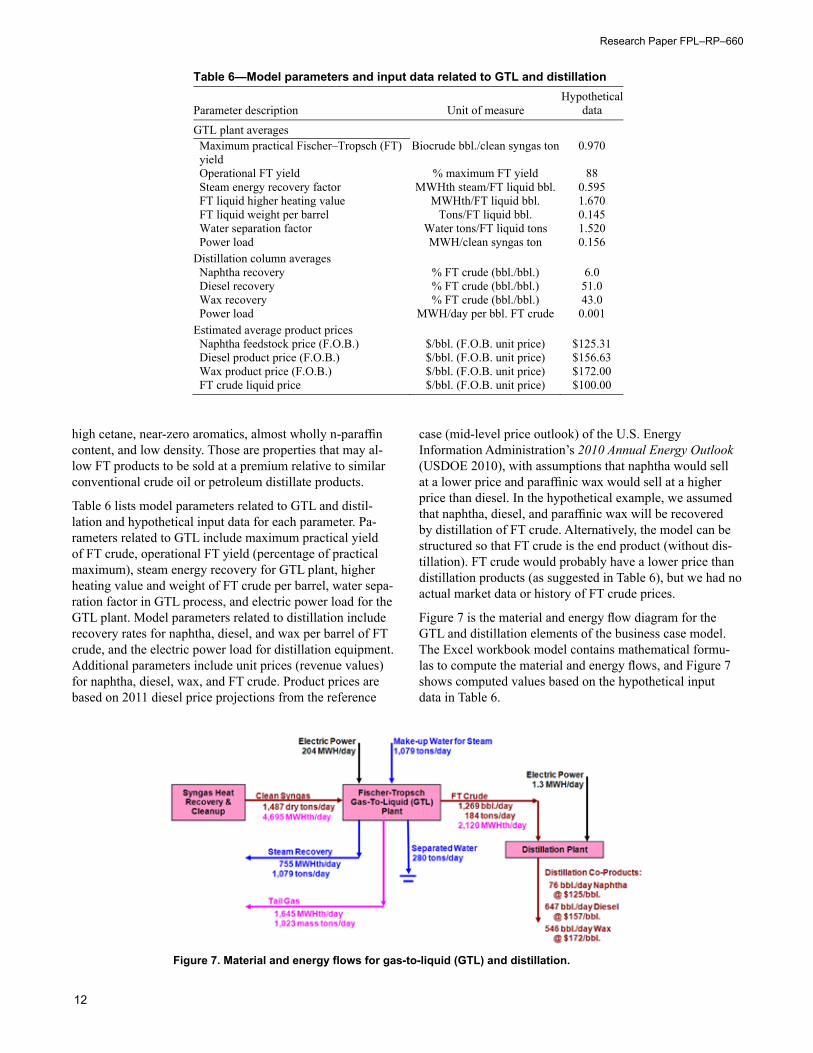
Table 6 lists model parameters related to GTL and distil-lation and hypothetical input data for each parameter. Pa-rameters related to GTL include maximum practical yield of FT crude, operational FT yield (percentage of practical maximum), steam energy recovery for GTL plant, higher heating value and weight of FT crude per barrel, water sepa-ration factor in GTL process, and electric power load for the GTL plant. Model parameters related to distillation include recovery rates for naphtha, diesel, and wax per barrel of FT crude, and the electric power load for distillation equipment. Additional parameters include unit prices (revenue values) for naphtha, diesel, wax, and FT crude. Product prices are based on 2011 diesel price projections from the reference
case (mid-level price outlook) of the U.S. Energy Information Administration’s 2010 Annual Energy Outlook (USDOE 2010), with assumptions that naphtha would sell at a lower price and paraffinic wax would sell at a higher price than diesel. In the hypothetical example, we assumed that naphtha, diesel, and paraffinic wax will be recovered by distillation of FT crude. Alternatively, the model can be structured so that FT crude is the end product (without dis-tillation). FT crude would probably have a lower price than distillation products (as suggested in Table 6), but we had no actual market data or history of FT crude prices.
Figure 7 is the material and energy flow diagram for the GTL and distillation elements of the business case model. The Excel workbook model contains mathematical formu-las to compute the material and energy flows, and Figure 7 shows computed values based on the hypothetical input data in Table 6.
Table 6—Model parameters and input data related to GTL and distillation
Parameter description Unit of measure Hypothetical
data
GTL plant averages Maximum practical Fischer–Tropsch (FT) yield
Biocrude bbl./clean syngas ton 0.970
Operational FT yield % maximum FT yield 88 Steam energy recovery factor MWHth steam/FT liquid bbl. 0.595 FT liquid higher heating value MWHth/FT liquid bbl. 1.670 FT liquid weight per barrel Tons/FT liquid bbl. 0.145 Water separation factor Water tons/FT liquid tons 1.520 Power load MWH/clean syngas ton 0.156
Distillation column averages Naphtha recovery % FT crude (bbl./bbl.) 6.0 Diesel recovery % FT crude (bbl./bbl.) 51.0 Wax recovery % FT crude (bbl./bbl.) 43.0 Power load MWH/day per bbl. FT crude 0.001
Estimated average product prices Naphtha feedstock price (F.O.B.) $/bbl. (F.O.B. unit price) $125.31 Diesel product price (F.O.B.) $/bbl. (F.O.B. unit price) $156.63 Wax product price (F.O.B.) $/bbl. (F.O.B. unit price) $172.00 FT crude liquid price $/bbl. (F.O.B. unit price) $100.00
Figure 7. Material and energy flows for gas-to-liquid (GTL) and distillation.
Modeling Integrated Biomass Gasification Business Concepts
13
Energy System UpgradesAn integrated biomass gasification concept may include energy system upgrades to take advantage of synergies in combined heat and power production. Thus we designed the model so that capacity can be added for combined heat or power production, specifically added power boiler or com-bustion gas turbine capacity along with associated power generator and steam recovery capacity. Added boiler or gas turbine capacity may be based on combustion of surplus tail gas from the GTL plant or any type of additional purchased boiler fuel (the price of which is specified in Table 1). Add-ed combustion capacity may also increase the output capac-ity of steam, power, or flue gas available for biomass drying.
The business process model uses conditional logic to allo-cate combustion and generating capacity, based on require-ments for steam, power, and flue gas heat energy in the overall system. The model also determines whether added gas turbine and power boiler systems will be operated at lower or higher flue gas temperatures, the lower flue gas temperature (~ 137 °C/280 °F) increasing steam and power output, whereas the higher temperature (~ 371 °C/700 °F) yields hotter flue gas suitable for biomass drying but reduces steam and power output. In addition, the boiler and gas tur-bine shares of added capacity are specified as data inputs, so the model can represent any combination of added boiler or gas turbine capacity, with different specified steam and energy generating rates.
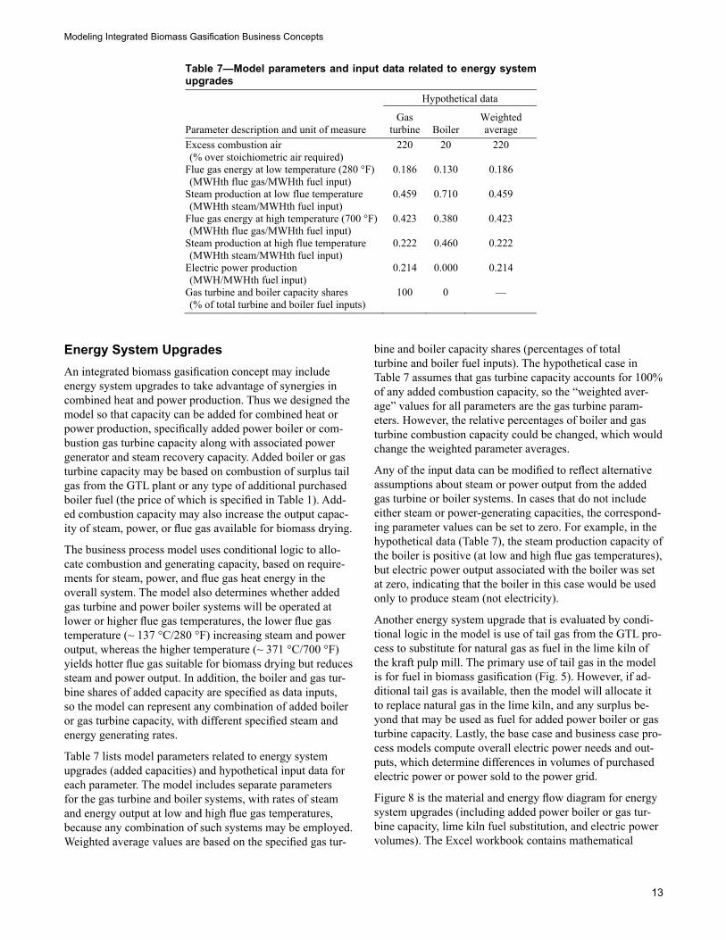
Table 7 lists model parameters related to energy system upgrades (added capacities) and hypothetical input data for each parameter. The model includes separate parameters for the gas turbine and boiler systems, with rates of steam and energy output at low and high flue gas temperatures, because any combination of such systems may be employed. Weighted average values are based on the specified gas tur-
bine and boiler capacity shares (percentages of total turbine and boiler fuel inputs). The hypothetical case in Table 7 assumes that gas turbine capacity accounts for 100% of any added combustion capacity, so the “weighted aver-age” values for all parameters are the gas turbine param-eters. However, the relative percentages of boiler and gas turbine combustion capacity could be changed, which would change the weighted parameter averages.
Any of the input data can be modified to reflect alternative assumptions about steam or power output from the added gas turbine or boiler systems. In cases that do not include either steam or power-generating capacities, the correspond-ing parameter values can be set to zero. For example, in the hypothetical data (Table 7), the steam production capacity of the boiler is positive (at low and high flue gas temperatures), but electric power output associated with the boiler was set at zero, indicating that the boiler in this case would be used only to produce steam (not electricity).
Another energy system upgrade that is evaluated by condi-tional logic in the model is use of tail gas from the GTL pro-cess to substitute for natural gas as fuel in the lime kiln of the kraft pulp mill. The primary use of tail gas in the model is for fuel in biomass gasification (Fig. 5). However, if ad-ditional tail gas is available, then the model will allocate it to replace natural gas in the lime kiln, and any surplus be-yond that may be used as fuel for added power boiler or gas turbine capacity. Lastly, the base case and business case pro-cess models compute overall electric power needs and out-puts, which determine differences in volumes of purchased electric power or power sold to the power grid.
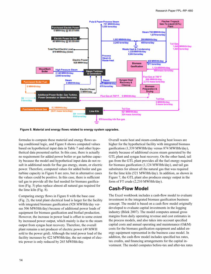
Figure 8 is the material and energy flow diagram for energy system upgrades (including added power boiler or gas tur-bine capacity, lime kiln fuel substitution, and electric power volumes). The Excel workbook contains mathematical
Table 7—Model parameters and input data related to energy systemupgrades
Hypothetical data
Parameter description and unit of measure Gas
turbine Boiler Weightedaverage
Excess combustion air 220 20 220 (% over stoichiometric air required)
Flue gas energy at low temperature (280 °F) 0.186 0.130 0.186 (MWHth flue gas/MWHth fuel input)
Steam production at low flue temperature 0.459 0.710 0.459 (MWHth steam/MWHth fuel input)
Flue gas energy at high temperature (700 °F) 0.423 0.380 0.423 (MWHth flue gas/MWHth fuel input)
Steam production at high flue temperature 0.222 0.460 0.222 (MWHth steam/MWHth fuel input)
Electric power production 0.214 0.000 0.214 (MWH/MWHth fuel input)
Gas turbine and boiler capacity shares 100 0 — (% of total turbine and boiler fuel inputs)
Research Paper FPL–RP–660
14
formulas to compute these material and energy flows us-ing conditional logic, and Figure 8 shows computed values based on hypothetical input data in Table 7 and other hypo-thetical data presented earlier. In this case, there is actually no requirement for added power boiler or gas turbine capac-ity because the model and hypothetical input data do not re-sult in additional needs for flue gas energy, steam, or electric power. Therefore, computed values for added boiler and gas turbine capacity in Figure 8 are zero, but in alternative cases the values could be positive. In this case, there is sufficient tail gas to provide all the fuel needed for biomass gasifica-tion (Fig. 5) plus replace almost all natural gas required for the lime kiln (Fig. 8).
Comparing energy flows in Figure 8 with the base case (Fig. 2), the total plant electrical load is larger for the facility with integrated biomass gasification (928 MWHth/day ver-sus 506 MWHth/day) because of additional power loads of equipment for biomass gasification and biofuel production. However, the increase in power load is offset to some extent by increased power output, which mainly is due to the steam output from syngas heat recovery. Therefore, the overall plant remains a net producer of electric power (49 MWH sold to the power grid). Although the total power load of the facility increases by 422 MWHth/day, the net output of elec-tric power is only reduced by 265 MWHth/day.
Overall waste heat and steam-condensing heat losses are higher for the hypothetical facility with integrated biomass gasification (1,339 MWHth/day versus 874 MWHth/day), mainly because of additional excess steam generated by the GTL plant and syngas heat recovery. On the other hand, tail gas from the GTL plant provides all the fuel energy required for biomass gasification (1,124 MWHth/day), and tail gas substitutes for almost all the natural gas that was required for the lime kiln (521 MWHth/day). In addition, as shown in Figure 7, the GTL plant also produces energy output in the form of FT crude (2,210 MWHth/day).
Cash-Flow ModelThe Excel workbook includes a cash-flow model to evaluate investment in the integrated biomass gasification business concept. The model is based on a cash flow model originally developed to evaluate capital investments in the logging industry (Bilek 2007). The model computes annual gross margins from daily operating revenue and cost estimates in the process models, and also takes into account specified capital costs and annual operating and maintenance (O&M) costs for the biomass gasification equipment and added en-ergy equipment represented in the business case model. In addition, the cash-flow model includes specified tax rates, tax credits, and financing arrangements for the capital in-vestment. The model computes before-tax and after-tax rates
Figure 8. Material and energy flows related to energy system upgrades.
Modeling Integrated Biomass Gasification Business Concepts
15
of return and net present value of investment in the business concept.
Annual Operating Costs and RevenueThe Excel workbook automatically computes projected op-erating revenue (or cost) impacts of the integrated biomass gasification concept by using projected daily revenue and operating costs from the process models and a specified number of operating days per year. The operating revenue (or cost) impact takes into account projected change in the gross margin of the overall enterprise that results from intro-duction of the integrated biomass gasification concept. Thus, the annual operating revenue (or cost) impact is the differ-ence between annual gross margins for the business case and the base case, minus annual O&M costs for the added biomass gasification and energy equipment, and also minus any other specified incremental process operating costs (Eq. (1)).
Annual Incremental Operating Revenue (or Cost) Impact = (Business Case Gross Margin) – (Base Case Gross Margin)
– (O&M Costs for Gasification and Energy Equipment)
– (Other Incremental Process Operating Costs) (1)
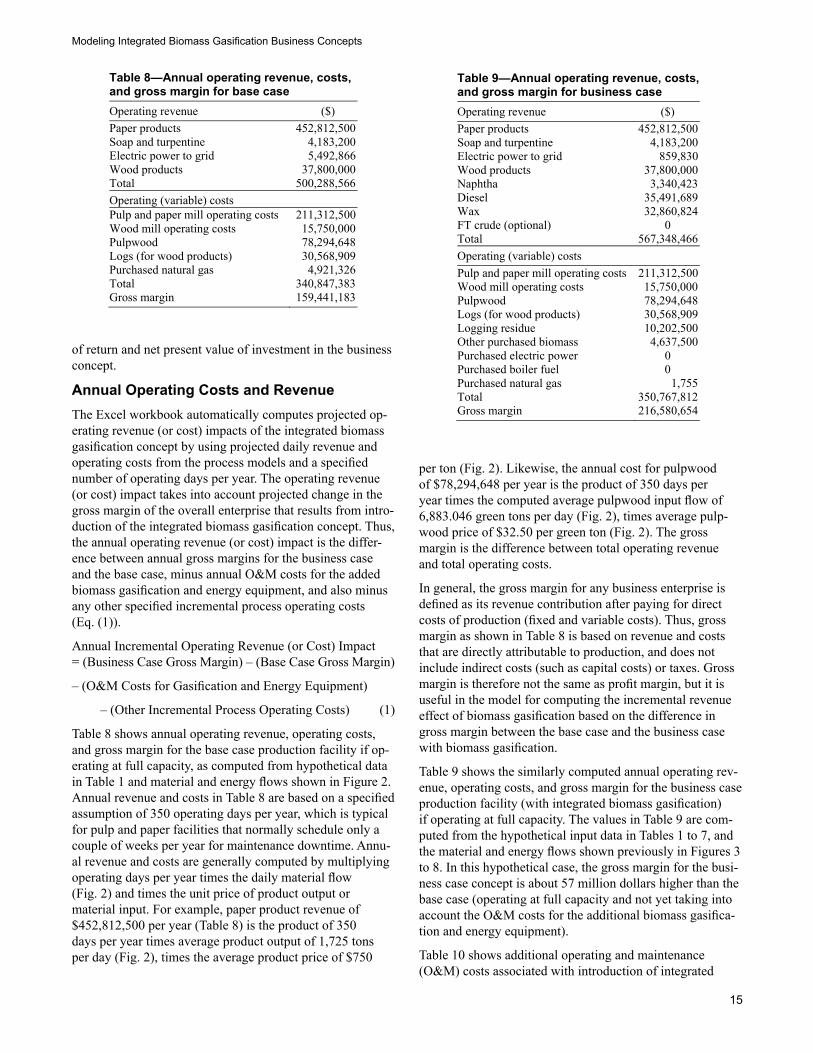
Table 8 shows annual operating revenue, operating costs, and gross margin for the base case production facility if op-erating at full capacity, as computed from hypothetical data in Table 1 and material and energy flows shown in Figure 2. Annual revenue and costs in Table 8 are based on a specified assumption of 350 operating days per year, which is typical for pulp and paper facilities that normally schedule only a couple of weeks per year for maintenance downtime. Annu-al revenue and costs are generally computed by multiplying operating days per year times the daily material flow (Fig. 2) and times the unit price of product output or material input. For example, paper product revenue of $452,812,500 per year (Table 8) is the product of 350 days per year times average product output of 1,725 tons per day (Fig. 2), times the average product price of $750
per ton (Fig. 2). Likewise, the annual cost for pulpwood of $78,294,648 per year is the product of 350 days per year times the computed average pulpwood input flow of 6,883.046 green tons per day (Fig. 2), times average pulp-wood price of $32.50 per green ton (Fig. 2). The gross margin is the difference between total operating revenue and total operating costs.
In general, the gross margin for any business enterprise is defined as its revenue contribution after paying for direct costs of production (fixed and variable costs). Thus, gross margin as shown in Table 8 is based on revenue and costs that are directly attributable to production, and does not include indirect costs (such as capital costs) or taxes. Gross margin is therefore not the same as profit margin, but it is useful in the model for computing the incremental revenue effect of biomass gasification based on the difference in gross margin between the base case and the business case with biomass gasification.
Table 9 shows the similarly computed annual operating rev-enue, operating costs, and gross margin for the business case production facility (with integrated biomass gasification) if operating at full capacity. The values in Table 9 are com-puted from the hypothetical input data in Tables 1 to 7, and the material and energy flows shown previously in Figures 3 to 8. In this hypothetical case, the gross margin for the busi-ness case concept is about 57 million dollars higher than the base case (operating at full capacity and not yet taking into account the O&M costs for the additional biomass gasifica-tion and energy equipment).
Table 10 shows additional operating and maintenance (O&M) costs associated with introduction of integrated
Table 8—Annual operating revenue, costs, and gross margin for base case Operating revenue ($) Paper products 452,812,500 Soap and turpentine 4,183,200 Electric power to grid 5,492,866 Wood products 37,800,000 Total 500,288,566 Operating (variable) costs Pulp and paper mill operating costs 211,312,500 Wood mill operating costs 15,750,000 Pulpwood 78,294,648 Logs (for wood products) 30,568,909 Purchased natural gas 4,921,326 Total 340,847,383 Gross margin 159,441,183
Table 9—Annual operating revenue, costs,and gross margin for business case Operating revenue ($) Paper products 452,812,500Soap and turpentine 4,183,200Electric power to grid 859,830Wood products 37,800,000Naphtha 3,340,423Diesel 35,491,689Wax 32,860,824FT crude (optional) 0 Total 567,348,466Operating (variable) costs Pulp and paper mill operating costs 211,312,500Wood mill operating costs 15,750,000Pulpwood 78,294,648Logs (for wood products) 30,568,909Logging residue 10,202,500Other purchased biomass 4,637,500Purchased electric power 0 Purchased boiler fuel 0 Purchased natural gas 1,755Total 350,767,812Gross margin 216,580,654
Research Paper FPL–RP–660
16
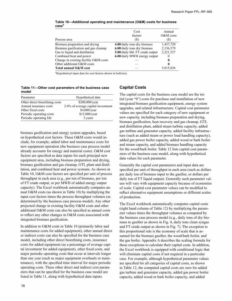
biomass gasification and energy system upgrades, based on hypothetical cost factors. These O&M costs would in-clude, for example, added labor and maintenance costs for new equipment operation (the business case process model already accounts for energy and material costs). O&M cost factors are specified as data inputs for each principal new equipment area, including biomass preparation and drying, biomass gasification and gas cleanup, GTL plant and distil-lation, and combined heat and power systems. As shown in Table 10, O&M cost factors are specified per unit of process throughput in each area (e.g., per ton of biomass, per ton of FT crude output, or per MWH of added energy output capacity). The Excel workbook automatically computes an-nual O&M costs (as shown in Table 10) by multiplying the input cost factors times the process throughput volumes (as determined by the business case process model). Any other projected change in existing facility O&M costs and other additional O&M costs can also be specified as annual costs to reflect any other changes in O&M costs associated with integrated biomass gasification.
In addition to O&M costs in Table 10 (primarily labor and maintenance costs for added equipment), other annual direct or indirect costs can also be specified for the business case model, including other direct biorefining costs, insurance costs for added equipment (as a percentage of average capi-tal investment for added equipment), other fixed costs, and major periodic operating costs that occur at intervals longer than one year (such as major equipment overhauls or main-tenance), with the specified time interval for major periodic operating costs. These other direct and indirect cost param-eters that can be specified for the business case model are listed in Table 11, along with hypothetical data inputs.
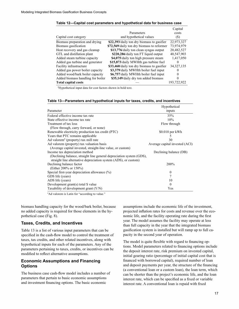
Capital CostsThe capital costs for the business case model are the ini-tial (year “0”) costs for purchase and installation of new integrated biomass gasification equipment, energy system upgrades, and related infrastructure. Capital cost parameter values are specified for each category of new equipment or new capacity, including biomass preparation and drying, biomass gasification, heat recovery and gas cleanup, GTL and distillation plant, added steam turbine capacity, added gas turbine and generator capacity, added facility infrastruc-ture (such as added steam or power load handling capacity), added gas power boiler capacity, added wood or bark boiler and steam capacity, and added biomass handling capacity for the wood/bark boiler. Table 12 lists capital cost param-eters of the business case model, along with hypothetical data values for each parameter.
Generally the capital cost parameters and input data are specified per unit of throughput in each area (such as dollars per daily ton of biomass input to the gasifier, or dollars per daily ton of FT liquid output). Generally such parameter val-ues will vary with equipment capacity because of economies of scale. Capital cost parameter values can be modified to reflect alternative equipment assumptions or different scales of production.
The Excel workbook automatically computes capital costs (right hand column of Table 12) by multiplying the param-eter values times the throughput volumes as computed by the business case process model (e.g., daily tons of dry bio-mass to gasifier as shown in Fig. 4, daily tons clean syngas and FT crude output as shown in Fig. 7). The exception to this proportional rule is the economy of scale that is as-sumed for the biomass gasifier, the wood/bark boiler, and the gas boiler. Appendix A describes the scaling formula for these exceptions to calculate their capital costs. In addition, the Excel workbook is equipped with conditional logic that will eliminate capital costs if not required in a particular case. For example, although hypothetical parameter values are specified for all categories of capital costs, as shown in Table 12, the computed capital costs are zero for added gas turbine and generator capacity, added gas power boiler capacity, added wood or bark boiler capacity, and added
Table 10—Additional operating and maintenance (O&M) costs for business casea
Process area
Costfactors
($)
AnnualO&M costs
($)Biomass preparation and drying 4.00/daily tons dry biomass 1,437,720 Biomass gasification and gas cleanup 6.00/daily tons dry biomass 2,156,579 Gas to liquid and distillation 5.00/daily bbl. FT crude output 2,221,527 Combined heat and power 6.00/daily MWH energy output 0 Change in existing facility O&M costs — 0Other additional O&M costs — 0Total annual O&M cost — 5,815,826 aHypothetical input data for cost factors shown in bold text.
Table 11—Other cost parameters of the business case model Parameter Hypothetical data Other direct biorefining costs $200,000/year Annual insurance costs 2.0% of average capital investmentOther fixed costs $4,000/year Periodic operating costs $15,000/year Periodic operating life 3 years
Modeling Integrated Biomass Gasification Business Concepts
17
biomass handling capacity for the wood/bark boiler, because no added capacity is required for those elements in the hy-pothetical case (Fig. 8).
Taxes, Credits, and IncentivesTable 13 is a list of various input parameters that can be specified in the cash-flow model to control the treatment of taxes, tax credits, and other related incentives, along with hypothetical inputs for each of the parameters. Any of the parameters pertaining to taxes, credits, or incentives can be modified to reflect alternative assumptions.
Economic Assumptions and Financing OptionsThe business case cash-flow model includes a number of parameters that pertain to basic economic assumptions and investment financing options. The basic economic
assumptions include the economic life of the investment, projected inflation rates for costs and revenue over the eco-nomic life, and the facility operating rate during the first year. The model assumes the facility may operate at less than full capacity in the year that the integrated biomass gasification system is installed but will ramp up to full ca-pacity in the second year of operation.
The model is quite flexible with regard to financing op-tions. Model parameters related to financing options include the deposit interest rate, risk premium on invested capital, initial gearing ratio (percentage of initial capital cost that is financed with borrowed capital), required number of loan and deposit payments per year, the structure of the financing (a conventional loan or a custom loan), the loan term, which can be shorter than the project’s economic life, and the loan interest rate, which can be specified as a fixed or variable interest rate. A conventional loan is repaid with fixed
Table 12—Capital cost parameters and hypothetical data for business case
Capital cost category Parameters
and hypothetical values
Capital costs ($)
Biomass preparation and drying $22,393/daily ton dry biomass to gasifier 22,973,327 Biomass gasification $72,569/daily ton dry biomass to reformer 73,974,979 Heat recovery and gas cleanup $13,776/daily ton clean syngas output 20,482,527 GTL and distillation plant $220,286/daily ton FT liquid output 40,547,903 Added steam turbine capacity $4,075/daily ton high pressure steam 1,417,050 Added gas turbine and generator $15,873/daily MWHth gas turbine fuel 0 Facility infrastructure $33,460/daily ton dry biomass to gasifier 34,327,135 Added gas power boiler capacity $3,379/daily MWHth boiler fuel input 0 Added wood/bark boiler capacity $6,757/daily MWHth boiler fuel input 0 Added biomass handling for boiler $35,149/daily dry ton added biomass 0 Total capital costs — 193,722,922
aHypothetical input data for cost factors shown in bold text.
Table 13—Parameters and hypothetical inputs for taxes, credits, and incentives
Parameter Hypothetical
inputsFederal effective income tax rate 35% State effective income tax rate 10% Treatment of tax loss Flow through
(Flow through, carry forward, or none) Renewable electricity production tax credit (PTC) $0.010 per kWh Years that PTC remains applicable 5 Ad valorema (property) tax mill rate 30 Ad valorem (property) tax valuation basis Average capital invested (ACI)
(Average capital invested, straight-line value, or custom) Income tax depreciation method Declining balance (DB)
(Declining balance, straight line general depreciation system (GDS), straight line alternative depreciation system (ADS), or custom)
Declining balance factor 200% (Either 200% or 150%)
Special first-year depreciation allowance (%) 0 GDS life (years) 7 ADS life (years) 10 Development grant(s) total $ value 0 Taxability of development grant (Y/N) Yes aAd valorem is Latin for “according to value.”
Research Paper FPL–RP–660
18
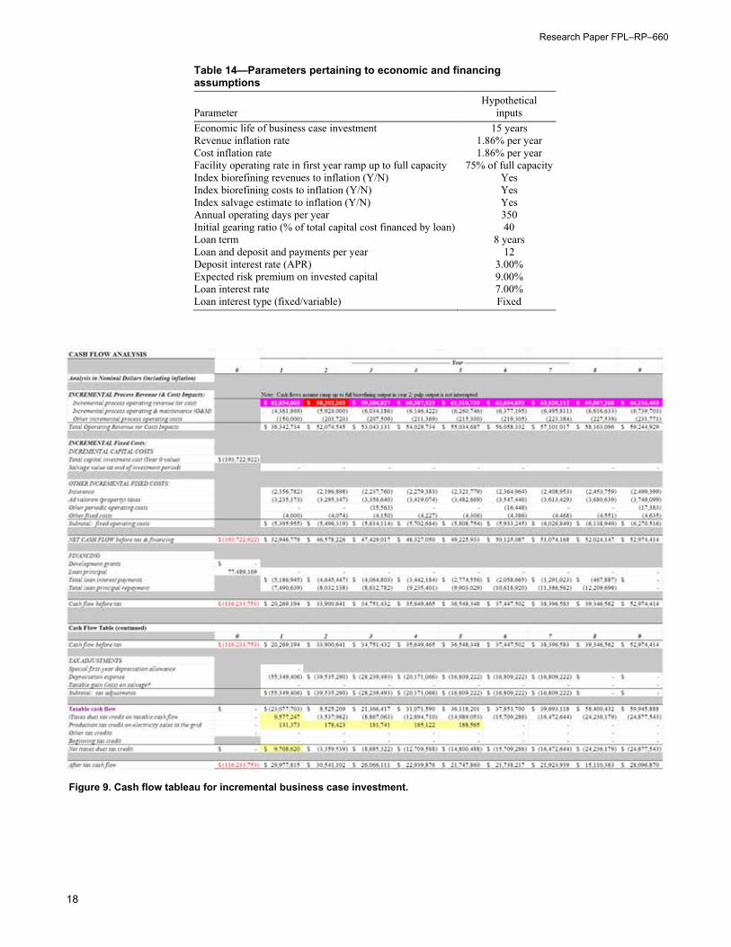
Table 14—Parameters pertaining to economic and financing assumptions
Parameter Hypothetical
inputsEconomic life of business case investment 15 years Revenue inflation rate 1.86% per year Cost inflation rate 1.86% per year Facility operating rate in first year ramp up to full capacity 75% of full capacity Index biorefining revenues to inflation (Y/N) Yes Index biorefining costs to inflation (Y/N) Yes Index salvage estimate to inflation (Y/N) Yes Annual operating days per year 350 Initial gearing ratio (% of total capital cost financed by loan) 40 Loan term 8 years Loan and deposit and payments per year 12 Deposit interest rate (APR) 3.00% Expected risk premium on invested capital 9.00% Loan interest rate 7.00% Loan interest type (fixed/variable) Fixed
Figure 9. Cash flow tableau for incremental business case investment.

Modeling Integrated Biomass Gasification Business Concepts
19
payments at the specified loan interest rate over the specified term. A custom loan can be structured any way the analyst wishes with interest payments and principal repayments entered for each year. Using the custom loan option, the analyst can explore the effect of different financing patterns (e.g., an interest-only loan for a specified number of years with a refinancing into a conventional loan).
Table 14 lists the parameters pertaining to economic and financing assumptions that can be specified in the cash-flow model, along with hypothetical inputs for each parameter. Note that the revenue and cost inflation rates in the sample data are based on inflation rate projections of the U.S. En-ergy Information Administration’s 2010 Annual Energy Out-look (USDOE 2010). Also, if user selections mean that some parameters are not needed, then these cells will receive gray shading. For example, if the loan repayment schedule is “Custom,” then the loan term and the parameters relating to the loan interest rate will be grayed out.
Of course, any of the parameter values can be modified to reflect alternative assumptions. Users will probably want to pay particular attention to the interest rate, financing, and risk premium assumptions.
Incremental Cash FlowsThe cash-flow model in the Excel workbook automatically computes projected annual incremental cash flows for the business case investment, based on data inputs and process model computations. The projected cash flows are displayed in a tableau that provides a complete pro-forma accounting of all annual cash flows over the economic life of the invest-ment in nominal dollars (after taking into account specified inflation rates). The annual cash flows include projected incremental revenue impacts, fixed costs and capital costs, cash flows related to financing, net cash flows before tax, tax adjustments, and after-tax cash flows.
Figure 9 shows the annual cash flow tableau for the incre-mental investment as computed by the cash-flow model in
Figure 9. (con.) Cash flow tableau for incremental business case investment.
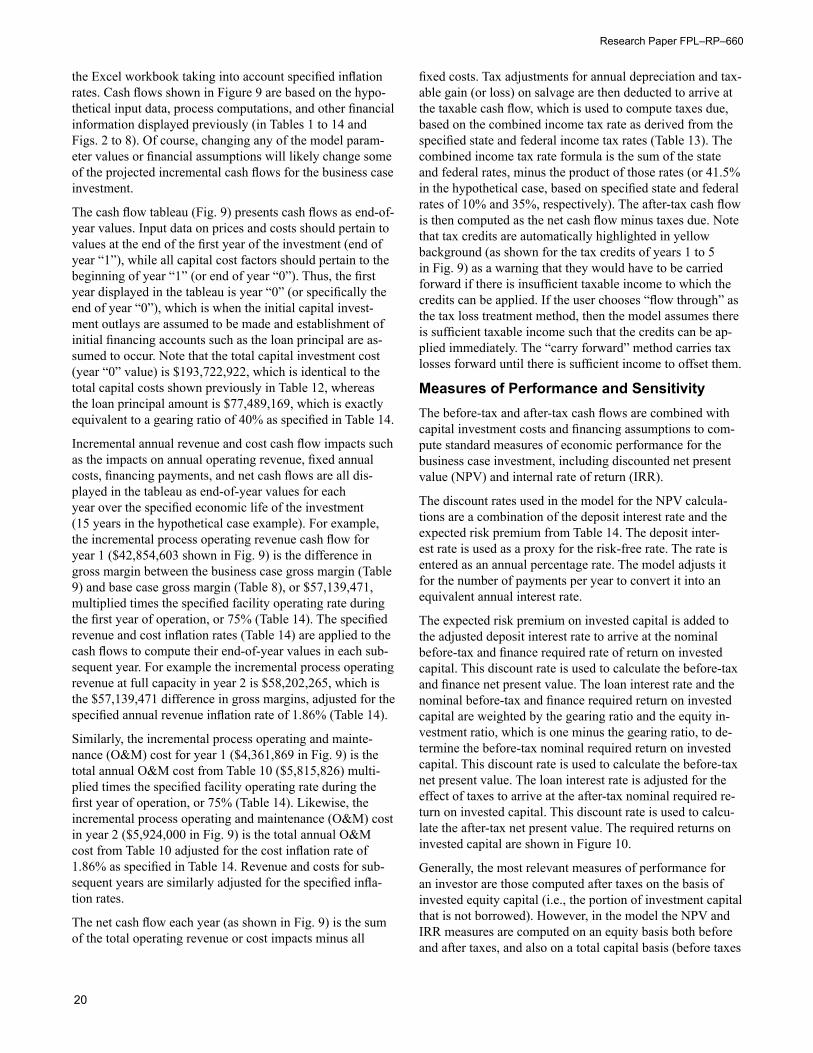
Research Paper FPL–RP–660
20
the Excel workbook taking into account specified inflation rates. Cash flows shown in Figure 9 are based on the hypo-thetical input data, process computations, and other financial information displayed previously (in Tables 1 to 14 and Figs. 2 to 8). Of course, changing any of the model param-eter values or financial assumptions will likely change some of the projected incremental cash flows for the business case investment.
The cash flow tableau (Fig. 9) presents cash flows as end-of-year values. Input data on prices and costs should pertain to values at the end of the first year of the investment (end of year “1”), while all capital cost factors should pertain to the beginning of year “1” (or end of year “0”). Thus, the first year displayed in the tableau is year “0” (or specifically the end of year “0”), which is when the initial capital invest-ment outlays are assumed to be made and establishment of initial financing accounts such as the loan principal are as-sumed to occur. Note that the total capital investment cost (year “0” value) is $193,722,922, which is identical to the total capital costs shown previously in Table 12, whereas the loan principal amount is $77,489,169, which is exactly equivalent to a gearing ratio of 40% as specified in Table 14.
Incremental annual revenue and cost cash flow impacts such as the impacts on annual operating revenue, fixed annual costs, financing payments, and net cash flows are all dis-played in the tableau as end-of-year values for each year over the specified economic life of the investment (15 years in the hypothetical case example). For example, the incremental process operating revenue cash flow for year 1 ($42,854,603 shown in Fig. 9) is the difference in gross margin between the business case gross margin (Table 9) and base case gross margin (Table 8), or $57,139,471, multiplied times the specified facility operating rate during the first year of operation, or 75% (Table 14). The specified revenue and cost inflation rates (Table 14) are applied to the cash flows to compute their end-of-year values in each sub-sequent year. For example the incremental process operating revenue at full capacity in year 2 is $58,202,265, which is the $57,139,471 difference in gross margins, adjusted for the specified annual revenue inflation rate of 1.86% (Table 14).
Similarly, the incremental process operating and mainte-nance (O&M) cost for year 1 ($4,361,869 in Fig. 9) is the total annual O&M cost from Table 10 ($5,815,826) multi-plied times the specified facility operating rate during the first year of operation, or 75% (Table 14). Likewise, the incremental process operating and maintenance (O&M) cost in year 2 ($5,924,000 in Fig. 9) is the total annual O&M cost from Table 10 adjusted for the cost inflation rate of 1.86% as specified in Table 14. Revenue and costs for sub-sequent years are similarly adjusted for the specified infla-tion rates.
The net cash flow each year (as shown in Fig. 9) is the sum of the total operating revenue or cost impacts minus all
fixed costs. Tax adjustments for annual depreciation and tax-able gain (or loss) on salvage are then deducted to arrive at the taxable cash flow, which is used to compute taxes due, based on the combined income tax rate as derived from the specified state and federal income tax rates (Table 13). The combined income tax rate formula is the sum of the state and federal rates, minus the product of those rates (or 41.5% in the hypothetical case, based on specified state and federal rates of 10% and 35%, respectively). The after-tax cash flow is then computed as the net cash flow minus taxes due. Note that tax credits are automatically highlighted in yellow background (as shown for the tax credits of years 1 to 5 in Fig. 9) as a warning that they would have to be carried forward if there is insufficient taxable income to which the credits can be applied. If the user chooses “flow through” as the tax loss treatment method, then the model assumes there is sufficient taxable income such that the credits can be ap-plied immediately. The “carry forward” method carries tax losses forward until there is sufficient income to offset them.
Measures of Performance and SensitivityThe before-tax and after-tax cash flows are combined with capital investment costs and financing assumptions to com-pute standard measures of economic performance for the business case investment, including discounted net present value (NPV) and internal rate of return (IRR).
The discount rates used in the model for the NPV calcula-tions are a combination of the deposit interest rate and the expected risk premium from Table 14. The deposit inter-est rate is used as a proxy for the risk-free rate. The rate is entered as an annual percentage rate. The model adjusts it for the number of payments per year to convert it into an equivalent annual interest rate.
The expected risk premium on invested capital is added to the adjusted deposit interest rate to arrive at the nominal before-tax and finance required rate of return on invested capital. This discount rate is used to calculate the before-tax and finance net present value. The loan interest rate and the nominal before-tax and finance required return on invested capital are weighted by the gearing ratio and the equity in-vestment ratio, which is one minus the gearing ratio, to de-termine the before-tax nominal required return on invested capital. This discount rate is used to calculate the before-tax net present value. The loan interest rate is adjusted for the effect of taxes to arrive at the after-tax nominal required re-turn on invested capital. This discount rate is used to calcu-late the after-tax net present value. The required returns on invested capital are shown in Figure 10.
Generally, the most relevant measures of performance for an investor are those computed after taxes on the basis of invested equity capital (i.e., the portion of investment capital that is not borrowed). However, in the model the NPV and IRR measures are computed on an equity basis both before and after taxes, and also on a total capital basis (before taxes
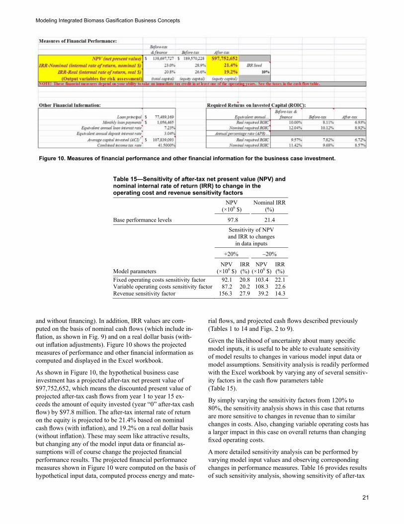
Modeling Integrated Biomass Gasification Business Concepts
21
and without financing). In addition, IRR values are com-puted on the basis of nominal cash flows (which include in-flation, as shown in Fig. 9) and on a real dollar basis (with-out inflation adjustments). Figure 10 shows the projected measures of performance and other financial information as computed and displayed in the Excel workbook.
As shown in Figure 10, the hypothetical business case investment has a projected after-tax net present value of $97,752,652, which means the discounted present value of projected after-tax cash flows from year 1 to year 15 ex-ceeds the amount of equity invested (year “0” after-tax cash flow) by $97.8 million. The after-tax internal rate of return on the equity is projected to be 21.4% based on nominal cash flows (with inflation), and 19.2% on a real dollar basis (without inflation). These may seem like attractive results, but changing any of the model input data or financial as-sumptions will of course change the projected financial performance results. The projected financial performance measures shown in Figure 10 were computed on the basis of hypothetical input data, computed process energy and mate-
rial flows, and projected cash flows described previously (Tables 1 to 14 and Figs. 2 to 9).
Given the likelihood of uncertainty about many specific model inputs, it is useful to be able to evaluate sensitivity of model results to changes in various model input data or model assumptions. Sensitivity analysis is readily performed with the Excel workbook by varying any of several sensitiv-ity factors in the cash flow parameters table (Table 15).
By simply varying the sensitivity factors from 120% to 80%, the sensitivity analysis shows in this case that returns are more sensitive to changes in revenue than to similar changes in costs. Also, changing variable operating costs has a larger impact in this case on overall returns than changing fixed operating costs.
A more detailed sensitivity analysis can be performed by varying model input values and observing corresponding changes in performance measures. Table 16 provides results of such sensitivity analysis, showing sensitivity of after-tax
Figure 10. Measures of financial performance and other financial information for the business case investment.
Table 15—Sensitivity of after-tax net present value (NPV) and nominal internal rate of return (IRR) to change in the operating cost and revenue sensitivity factors
NPV (×106 $)
Nominal IRR (%)
Base performance levels 97.8 21.4
Sensitivity of NPV and IRR to changes
in data inputs
+20% –20%
Model parameters NPV
(×106 $)IRR(%)
NPV(×106 $)
IRR(%)
Fixed operating costs sensitivity factor 92.1 20.8 103.4 22.1 Variable operating costs sensitivity factor 87.2 20.2 108.3 22.6 Revenue sensitivity factor 156.3 27.9 39.2 14.3
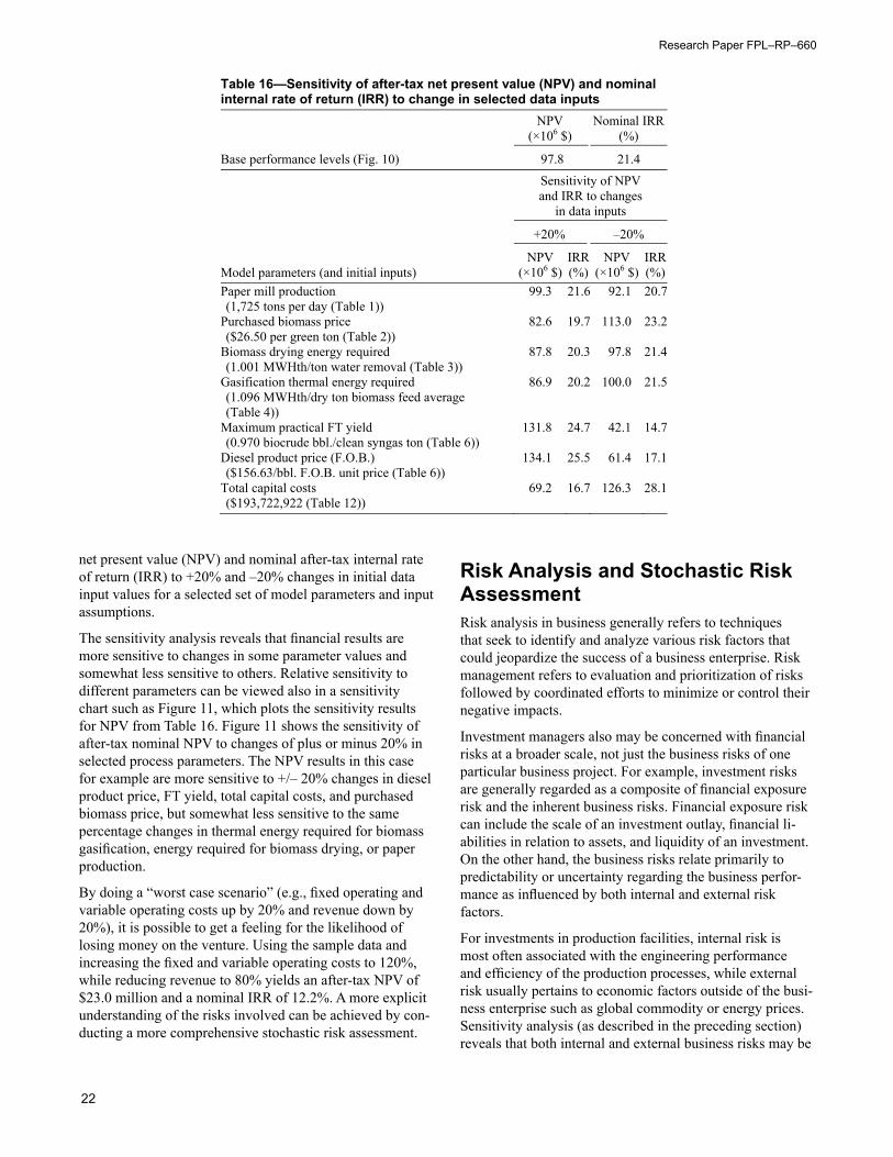
Research Paper FPL–RP–660
22
net present value (NPV) and nominal after-tax internal rate of return (IRR) to +20% and –20% changes in initial data input values for a selected set of model parameters and input assumptions.
The sensitivity analysis reveals that financial results are more sensitive to changes in some parameter values and somewhat less sensitive to others. Relative sensitivity to different parameters can be viewed also in a sensitivity chart such as Figure 11, which plots the sensitivity results for NPV from Table 16. Figure 11 shows the sensitivity of after-tax nominal NPV to changes of plus or minus 20% in selected process parameters. The NPV results in this case for example are more sensitive to +/– 20% changes in diesel product price, FT yield, total capital costs, and purchased biomass price, but somewhat less sensitive to the same percentage changes in thermal energy required for biomass gasification, energy required for biomass drying, or paper production.
By doing a “worst case scenario” (e.g., fixed operating and variable operating costs up by 20% and revenue down by 20%), it is possible to get a feeling for the likelihood of losing money on the venture. Using the sample data and increasing the fixed and variable operating costs to 120%, while reducing revenue to 80% yields an after-tax NPV of $23.0 million and a nominal IRR of 12.2%. A more explicit understanding of the risks involved can be achieved by con-ducting a more comprehensive stochastic risk assessment.
Risk Analysis and Stochastic Risk AssessmentRisk analysis in business generally refers to techniques that seek to identify and analyze various risk factors that could jeopardize the success of a business enterprise. Risk management refers to evaluation and prioritization of risks followed by coordinated efforts to minimize or control their negative impacts.
Investment managers also may be concerned with financial risks at a broader scale, not just the business risks of one particular business project. For example, investment risks are generally regarded as a composite of financial exposure risk and the inherent business risks. Financial exposure risk can include the scale of an investment outlay, financial li-abilities in relation to assets, and liquidity of an investment. On the other hand, the business risks relate primarily to predictability or uncertainty regarding the business perfor-mance as influenced by both internal and external risk factors.
For investments in production facilities, internal risk is most often associated with the engineering performance and efficiency of the production processes, while external risk usually pertains to economic factors outside of the busi-ness enterprise such as global commodity or energy prices. Sensitivity analysis (as described in the preceding section) reveals that both internal and external business risks may be
Table 16—Sensitivity of after-tax net present value (NPV) and nominal internal rate of return (IRR) to change in selected data inputs
NPV (×106 $)
Nominal IRR (%)
Base performance levels (Fig. 10) 97.8 21.4 Sensitivity of NPV and IRR to changes
in data inputs
+20% –20%
Model parameters (and initial inputs) NPV
(×106 $)IRR(%)
NPV (×106 $)
IRR(%)
Paper mill production 99.3 21.6 92.1 20.7(1,725 tons per day (Table 1))
Purchased biomass price 82.6 19.7 113.0 23.2($26.50 per green ton (Table 2))
Biomass drying energy required 87.8 20.3 97.8 21.4(1.001 MWHth/ton water removal (Table 3))
Gasification thermal energy required 86.9 20.2 100.0 21.5(1.096 MWHth/dry ton biomass feed average (Table 4))
Maximum practical FT yield 131.8 24.7 42.1 14.7(0.970 biocrude bbl./clean syngas ton (Table 6))
Diesel product price (F.O.B.) 134.1 25.5 61.4 17.1($156.63/bbl. F.O.B. unit price (Table 6))
Total capital costs 69.2 16.7 126.3 28.1($193,722,922 (Table 12))
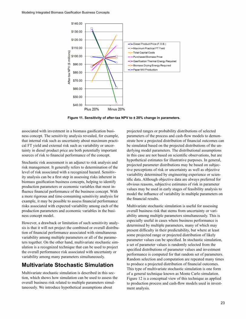
Modeling Integrated Biomass Gasification Business Concepts
23
associated with investment in a biomass gasification busi-ness concept. The sensitivity analysis revealed, for example, that internal risk such as uncertainty about maximum practi-cal FT yield and external risk such as variability or uncer-tainty in diesel product price are both potentially important sources of risk to financial performance of the concept.
Stochastic risk assessment is an adjunct to risk analysis and risk management. It generally refers to determination of the level of risk associated with a recognized hazard. Sensitiv-ity analysis can be a first step in assessing risks inherent in biomass gasification business concepts, helping to identify production parameters or economic variables that most in-fluence financial performance of the business concept. With a more rigorous and time-consuming sensitivity analysis for example, it may be possible to assess financial performance risks associated with expected variability among each of the production parameters and economic variables in the busi-ness concept model.
However, a drawback or limitation of such sensitivity analy-sis is that it will not project the combined or overall distribu-tion of financial performance associated with simultaneous variability among multiple parameters or all of the parame-ters together. On the other hand, multivariate stochastic sim-ulation is a recognized technique that can be used to project the overall performance risk associated with uncertainty or variability among many parameters simultaneously.
Multivariate Stochastic SimulationMultivariate stochastic simulation is described in this sec-tion, which shows how simulation can be used to assess the overall business risk related to multiple parameters simul-taneously. We introduce hypothetical assumptions about
projected ranges or probability distributions of selected parameters of the process and cash-flow models to demon-strate how a projected distribution of financial outcomes can be simulated based on the projected distributions of the un-derlying model parameters. The distributional assumptions in this case are not based on scientific observations, but are hypothetical estimates for illustrative purposes. In general, projected parameter distributions may be based on subjec-tive perceptions of risk or uncertainty as well as objective variability determined by engineering experience or scien-tific data. Although objective data are always preferred for obvious reasons, subjective estimates of risk in parameter values may be used in early stages of feasibility analysis to model the influence of variability in multiple parameters on the financial results.
Multivariate stochastic simulation is useful for assessing overall business risk that stems from uncertainty or vari-ability among multiple parameters simultaneously. This is especially useful in cases where business performance is determined by multiple parameters, many of which may present difficulty in their predictability, but where at least some projected range or projected distribution of likely parameter values can be specified. In stochastic simulation, a set of parameter values is randomly selected from the specified distributions of parameter values and investment performance is computed for that random set of parameters. Random selection and computation are repeated many times to produce a projected distribution of financial outcomes. This type of multivariate stochastic simulation is one form of a general technique known as Monte Carlo simulation. Figure 12 is a conceptual view of this technique as applied to production process and cash-flow models used in invest-ment analysis.
Figure 11. Sensitivity of after-tax NPV to ± 20% change in parameters.

Research Paper FPL–RP–660
24
Various computer programs are available to assist in per-forming Monte Carlo or multivariate stochastic simulation, and various commercially available software packages can perform multivariate stochastic simulations on models built in Excel workbooks. We used one such program, @RISK version 4.5, which is distributed by the Palisade Corporation (Ithaca, New York). We used @RISK to run multivariate stochastic simulations of investment performance based on our Excel model of the integrated biomass gasification busi-ness concept. The @RISK software allows the user to spec-ify different types of distributional assumptions for model input parameters, ranging from uniform data distributions to various types of statistical distributions. After the user speci-fies distributional assumptions for input parameters, the user can run a Monte Carlo simulation with the Excel model to compute the projected distribution of model results (finan-cial performance measures) based on all of the distributional assumptions for input parameters. As illustrated conceptu-ally in Figure 12, the simulation translates distributional assumptions about input parameters into the projected distri-bution of investment performance.
To provide an example of risk assessment based on mul-tivariate stochastic simulation, we developed hypotheti-cal distributions of values for selected parameters in the integrated biomass gasification models. To compare risk assessment with sensitivity analysis, we focused the risk as-sessment on the same set of parameters we used to illustrate sensitivity analysis (Table 16). Of course, any other set of model parameters may be selected as the focus of risk as-sessment, not just those that we selected here.
Table 17 lists model parameters selected for stochastic simu-lation, along with hypothetical distributions that we speci-fied for each parameter. We specified a uniform distribution for projected paper mill production, with a range from 1,600 to 1,700 tons per day of average output volume. This range of projected production is somewhat less than the mill ca-pacity (1,725 tons per day) on the assumption that variable market demands would reduce average mill output volume to something less than mill capacity on average (here the range is from about 93% to 99% of capacity). The uniform
distribution means average production volume over the life of the investment could assume any value within that range at a uniform or equal likelihood of occurrence.
For many of the other model parameters, we specified a nor-mal distribution, which tends to be a reasonable assumption for many economic or engineering parameters (although of course other distributional assumptions can be used if more accurate or better supported by actual data). The normal dis-tributions are defined by simply specifying their projected mean values and standard deviations. The width of a 95% confidence interval is approximately two standard devia-tions on either side of the mean value for a normally distrib-uted parameter. For example, for purchased biomass price we specified a hypothetical mean value of $26.50 per ton and a standard deviation of $2.50 per ton, which means that average biomass price over the life of the investment (before inflation) is projected to have approximately a 95% likeli-hood of being within a range from around $21.50 to $31.50 per ton (with a central tendency or higher likelihood of being closer to the mean value). For most of the variables that were assumed to be normally distributed, the hypotheti-cal standard deviation was specified to be 10% of the mean value. However, in the case of diesel product price, the mean value and standard deviation were based on energy price projections from the 2009 Annual Energy Outlook (Energy Information Administration, U.S. Department of Energy).
It is possible, of course, to project other alternative distribu-tions, including uneven distributions, such as the Weibull distribution. For example, we specified a Weibull distribu-tion for total capital costs, using a distributional adjustment with Weibull parameters of α = 1.5 and β = 0.5, and mini-mum value at 70% of the initial capital cost. This resulted in a skewed distribution for projected capital costs, ranging from 30% below the initial capital cost estimate to a wider range of values above that estimate. This type of skewed distribution could be used, for example, to reflect a subjec-tive perception that actual capital costs would likely escalate (or would have been underestimated) rather than vice versa. Under the Weibull distribution assumptions, the mean value
Figure 12. Conceptual view of simulation applied to investment analysis.

Modeling Integrated Biomass Gasification Business Concepts
25
of projected capital costs becomes $224 million, and the 95% confidence interval extends from $149 million (or 77% of initial capital cost) to $337 million (174% of initial capi-tal cost).
Figure 13 illustrates the hypothetical probability density charts and shows the 95% confidence intervals for each of the parameters, as specified by the distributional assump-tions in Table 17.
Using the @RISK software, we ran a multivariate Monte Carlo stochastic simulation of investment performance based on our Excel model of the integrated biomass gasification business concept along with all of the distri-butional assumptions for selected parameters as specified in Table 17 and Figure 13. The Monte Carlo simulation was run with 1,000 iterations. Figure 14 shows simulation
Table 17—Selected model parameters and hypothetical distributions Model parameters (and initial values) Hypothetical distributions Paper mill production Uniform Range: 1,600 – 1,700 (Tons per day (Table 1))
Purchased biomass price Normal Mean: 26.50, St. Dev.: 2.50 ($ per green ton (Table 2))
Biomass drying energy required Normal Mean: 1.001, St. Dev.: 0.10 (MWHth/ton water removal (Table 3))
Gasification thermal energy required Normal Mean: 1.096, St. Dev.: 0.11 (MWHth/dry ton biomass feed average (Table 4))
Maximum practical FT yield Normal Mean: 0.970, St. Dev.: 0.10 (Biocrude bbl./clean syngas ton (Table 6))
Diesel product price (F.O.B.) Normal Mean: 156.63, St. Dev.: 30.91 (($) per bbl. F.O.B. unit price (Table 6))
Total capital costs Weibull α = 1.5, β = 0.5, shift = 70% ($194 million (Table 12))
Figure 13. Probability density charts and 95% confidence intervals for hypothetical parameter distributions.
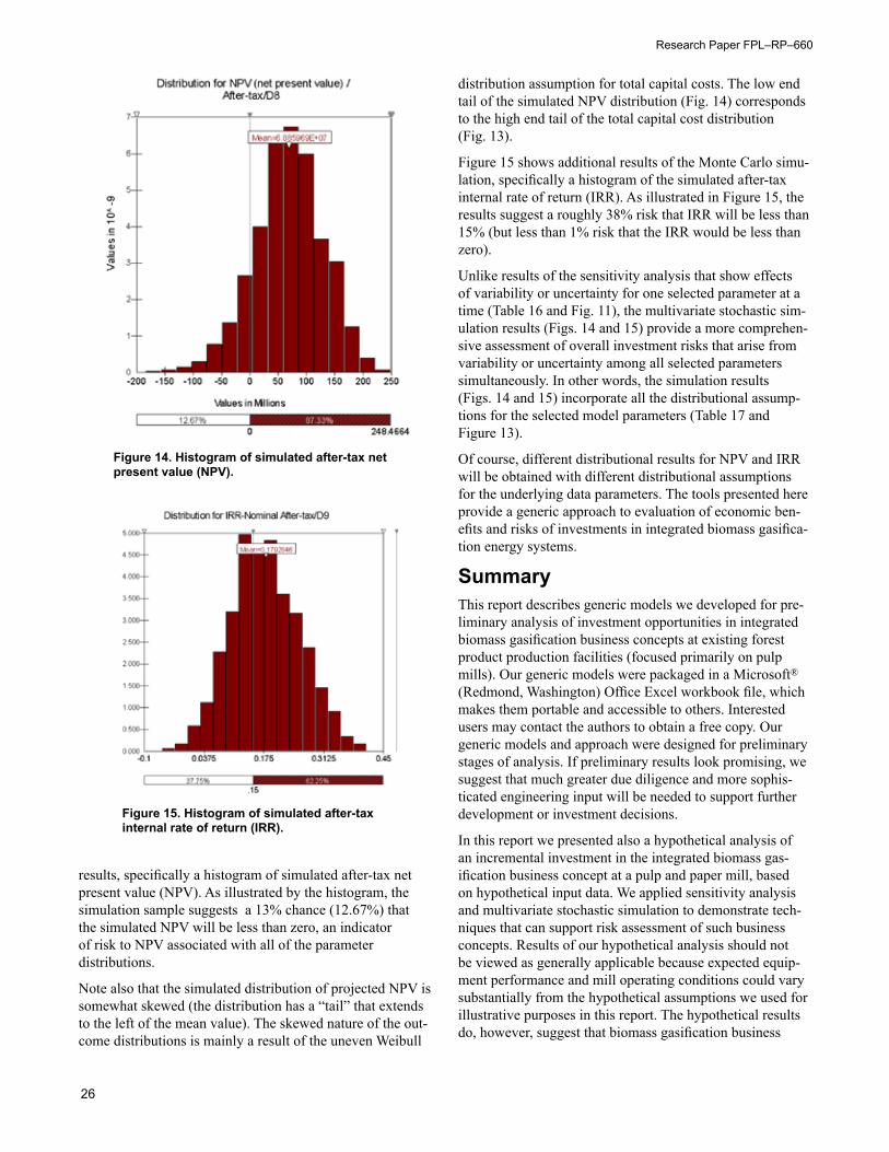
Research Paper FPL–RP–660
26
results, specifically a histogram of simulated after-tax net present value (NPV). As illustrated by the histogram, the simulation sample suggests a 13% chance (12.67%) that the simulated NPV will be less than zero, an indicator of risk to NPV associated with all of the parameter distributions.
Note also that the simulated distribution of projected NPV is somewhat skewed (the distribution has a “tail” that extends to the left of the mean value). The skewed nature of the out-come distributions is mainly a result of the uneven Weibull
distribution assumption for total capital costs. The low end tail of the simulated NPV distribution (Fig. 14) corresponds to the high end tail of the total capital cost distribution (Fig. 13).
Figure 15 shows additional results of the Monte Carlo simu-lation, specifically a histogram of the simulated after-tax internal rate of return (IRR). As illustrated in Figure 15, the results suggest a roughly 38% risk that IRR will be less than 15% (but less than 1% risk that the IRR would be less than zero).
Unlike results of the sensitivity analysis that show effects of variability or uncertainty for one selected parameter at a time (Table 16 and Fig. 11), the multivariate stochastic sim-ulation results (Figs. 14 and 15) provide a more comprehen-sive assessment of overall investment risks that arise from variability or uncertainty among all selected parameters simultaneously. In other words, the simulation results (Figs. 14 and 15) incorporate all the distributional assump-tions for the selected model parameters (Table 17 and Figure 13).
Of course, different distributional results for NPV and IRR will be obtained with different distributional assumptions for the underlying data parameters. The tools presented here provide a generic approach to evaluation of economic ben-efits and risks of investments in integrated biomass gasifica-tion energy systems.
SummaryThis report describes generic models we developed for pre-liminary analysis of investment opportunities in integrated biomass gasification business concepts at existing forest product production facilities (focused primarily on pulp mills). Our generic models were packaged in a Microsoft® (Redmond, Washington) Office Excel workbook file, which makes them portable and accessible to others. Interested users may contact the authors to obtain a free copy. Our generic models and approach were designed for preliminary stages of analysis. If preliminary results look promising, we suggest that much greater due diligence and more sophis-ticated engineering input will be needed to support further development or investment decisions.
In this report we presented also a hypothetical analysis of an incremental investment in the integrated biomass gas-ification business concept at a pulp and paper mill, based on hypothetical input data. We applied sensitivity analysis and multivariate stochastic simulation to demonstrate tech-niques that can support risk assessment of such business concepts. Results of our hypothetical analysis should not be viewed as generally applicable because expected equip-ment performance and mill operating conditions could vary substantially from the hypothetical assumptions we used for illustrative purposes in this report. The hypothetical results do, however, suggest that biomass gasification business
Figure 14. Histogram of simulated after-tax net present value (NPV).
Figure 15. Histogram of simulated after-tax internal rate of return (IRR).
Modeling Integrated Biomass Gasification Business Concepts
27
concepts could be economically attractive, and we recom-mend due diligence and careful quantitative evaluation of risks and investment performance to assess the concept in specific locations.
ReferencesAgenda 2020 CTO Working Group. 2008a. Adding biofuel/bioproduct capacity to existing U.S. mills; Part 1: Options. Norcross, GA: Paper 360° (TAPPI Press) Vol. 3, No. 4. (April 2008): 33–37.
Agenda 2020 CTO Working Group. 2008b. Adding biofuel/bioproduct capacity to existing U.S. mills; Part 2: The Busi-ness Case. Norcross, GA: Paper 360° (TAPPI Press) Vol. 3, No. 6. (June/July 2008): 24–28.
Aspen Plus®. 2000. Aspen Plus User Guide, Version 10.2. Cambridge, MA: Aspen Technology, Inc. 936 p.
Bilek, E.M. (Ted). 2007. ChargeOut! Determining machine and capital equipment charge-out rates using discounted cash-flow analysis. Gen. Tech. Rep. FPL–GTR–171. Madi-son, WI: U.S. Department of Agriculture, Forest Service, Forest Products Laboratory. 33 p.
Connor, E.J. 2007. The pathway to our bio-future. Cohasset, MA: PaperAge. (March/April 2007): 40–43.
Ince, P.J. 1979. How to estimate recoverable heat energy in wood or bark fuels. Gen. Tech. Rep. FPL–GTR–29. Madi-son, WI: U.S. Department of Agriculture, Forest Service, Forest Products Laboratory. 6 p.
Larson, E.D.; Consonni, S.; Katofsky, R.E.; Iisa, K.; Fred-erick, W.J., Jr. 2008. An assessment of gasification-based biorefining at kraft pulp and paper mills in the United States, Part A: Background and assumptions. TAPPI Journal. Vol. 7, No. 11. (November 2008): 8–14.
Larson, E.D.; Consonni, S.; Katofsky, R.E.; Iisa, K.; Fred-erick, W.J., Jr. 2009. An assessment of gasification-based biorefining at kraft pulp and paper mills in the United States, Part B: Results. TAPPI Journal. Vol. 8, No. 1. (January 2009): 27–35.
Niemantsverdriet, J.V. 2007. Modeling Fischer-Tropsch syn-thesis using density functional theory. Eindhoven,The Neth-erlands: Technical University of Eindhoven, Department of Chemical Engineering and Chemistry. (http://www.onder-zoekinformatie.nl/en/oi/nod/onderzoek/OND1315127/). (Accessed December 15, 2010).
Thorp, B.A.; Thorp, B.A., IV; Murdock-Thorp, L.D. 2008a. A compelling case for integrated biorefineries (Part I). Nor-cross, GA: Paper 360° (TAPPI Press) Vol. 3, No. 3. (March 2008): 14–15.
Thorp, B.A.; Thorp, B.A., IV; Murdock-Thorp, L.D. 2008b. A compelling case for integrated biorefineries (Part II). Nor-cross, GA: Paper 360° (TAPPI Press) Vol. 3, No. 4. (April 2008): 20–22.
Ulrich, G.D.; Vasudevan, P.T. 2004. Chemical engineering process design and economics: a practical guide. 2nd ed. Durham, NH: Process Publishing.
USDOE. 2010. Annual Energy Outlook 2010. Report #: DOE/EIA-0383. Washington, D.C.: U.S. Department of Energy. 221 p.
Zerbe, J.; Arola, R.; Wahlgren, H.G.; Rowell, R. 1976. The feasibility of utilizing forest residues for energy & chemi-cals. NSF–RA–760013, Contract No. NSF AER–75–19464. On file with: USDA Forest Service, Washington, DC.

Research Paper FPL–RP–660
28
Appendix A—Base Case Process Model RelationshipsSome examples of mathematical relationships in the base case process model are described in this appendix, which shows examples of how material and energy flows in the base case process diagram (Fig. 2) are computed in the Ex-cel worksheet based on sample input data (Table 1).
The average paper mill production (tons/day) and paper product revenue ($/ton) are model input parameters (Table 1). For those parameters, we specified a hypothetical production volume of 1,725 tons/day and average product value of $750/ton (corresponding to the hypothetical output capacity of a fairly large mill producing printing and writ-ing paper products). If a mill produces a variety of different products, the product output volume should be the total of all products, and the product revenue should be the weighted average for all products. Those parameter values appear also in the upper right corner of the base case process diagram as outputs of the paper mill (Fig. 2).
The base case model assumes that wood pulp output of the pulp mill is determined by on-site wood pulp produc-tion requirements of the paper mill, computed by taking into account average paper product moisture content and paper coatings and fillers content. The “coatings and fill-ers” content should include any recycled fiber or purchased market pulp fiber. The process diagram shows the average daily flow of wood pulp in air-dry tons (1,527 air-dry tons per day) computed from the specified paper output ton-nage, coatings and fillers content, and average machine-dry moisture content of the paper product. Hypothetical values that are typical for printing and writing paper products were specified for the coatings and fillers fraction (17%) and ma-chine-dry moisture content (4%), as shown in Table 1. Un-less otherwise noted, pulp, paper, and wood moisture con-tent parameters in the model are expressed on a total weight basis (weight of moisture as a percentage of the total weight of material and moisture), which is the standard method in the pulp and paper industry. The pulp output is computed according to the following equation (A-1), which includes the constant term (0.9) to take into account that wood pulp tonnage is generally measured on a standard “air-dry” basis, meaning specifically 10% moisture content:
Pulp Output = ((1– (Coatings and Fillers %)) × ((Paper Output Tons) × (1-Machine-dry moisture %))) ÷ 0.9
The input of clean pulp chips to the pulp mill (5,976 green tons/day, as shown in Fig. 2) is computed on the basis of a specified pulp yield parameter and pulp chip moisture con-tent (Table 1). Pulpwood inputs such as pulp chips at pulp mills are commonly measured on a “green” tonnage basis, meaning the total weight of the wood including moisture
content. The term “clean” is a term used in the industry that generally means the pulpwood has had bark removed and has been screened for removal of dirt, stones, or other debris. As shown in Table 1, a hypothetical value was speci-fied for pulp yield (46%) that is typical for pulp yield at a kraft pulp mill producing bleached kraft pulp for printing and writing paper. Pulp yields actually vary by pulping pro-cess and the type of paper product being produced, and may range from less than 50% for bleached chemical pulps to over 90% for mechanical pulps. By standard convention in the pulp industry, pulp yield refers to the recovery ratio of pulp per unit of wood input on a dry weight basis (excluding moisture) and is expressed as a percentage, the ratio of dry weight of pulp output to the dry weight of wood input to the pulping process. Some pulp mills may have multiple pulp-ing lines with different yields, and in that case the pulp yield parameter for the model should be specified as the weighted average pulp yield. A hypothetical value of 50% moisture content was specified for the pulp chip moisture content (Table 1). That moisture content level is commonly applied as an average assumption for the moisture content of pulp-wood, although wood moisture content can naturally vary by season, region, and wood species. The tonnage of clean pulp chips that are input to the pulp mill is computed by the following equation (A-2), which includes the constant term (0.9) to account for wood pulp tonnage being measured on a standard “air-dry” basis, meaning specifically 10% moisture content:
Clean Pulp Chips = ((Pulp Output) × 0.9 / (Pulp Yield)) ÷ (1 – (Pulp Chip
Moisture Content))
Recoverable wood soap, turpentine, and other resin extrac-tives are typical by-products of wood pulp mills. Soaps are the product of reaction between pulping chemical alkali and fatty acids from wood, whereas turpentine and other extrac-tives may be recovered prior to pulping in the pre-steaming of wood chips. Recovery potential can vary by wood species and by type of pulping process. The daily soap and turpen-tine outputs and related revenue of the pulp mill are com-puted on the basis of the tonnage of clean pulp chip inputs and specified average recovery and average revenue per ton of soap and turpentine. The soap and turpentine recovery and average revenue are model parameters that refer to total soap, turpentine, and other recoverable extractives. In the hypothetical input data, we specified a soap and turpentine recovery of 4.0 gallons per green ton of clean pulp chips and a soap and turpentine revenue of $0.50 per gallon recovered (Table 1).
Other aspects of the base case process are likely to change upon introducing the integrated gasification to biofuel busi-ness case process. One is the elimination of the wood/bark boiler when all or part of its biomass feedstock is directed to the gasification plant for the alternate generation of electric-ity and steam needed by the pulp mill. In some instances it
(A-1)
(A-2)
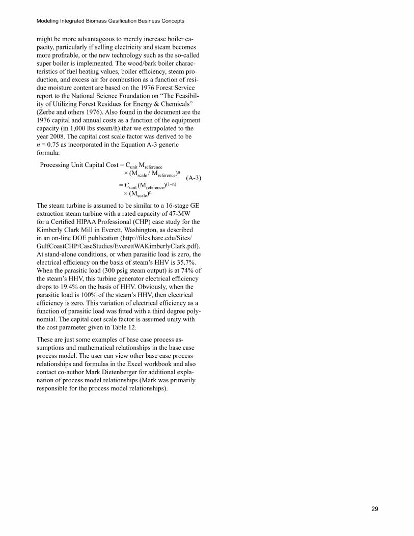
Modeling Integrated Biomass Gasification Business Concepts
29
might be more advantageous to merely increase boiler ca-pacity, particularly if selling electricity and steam becomes more profitable, or the new technology such as the so-called super boiler is implemented. The wood/bark boiler charac-teristics of fuel heating values, boiler efficiency, steam pro-duction, and excess air for combustion as a function of resi-due moisture content are based on the 1976 Forest Service report to the National Science Foundation on “The Feasibil-ity of Utilizing Forest Residues for Energy & Chemicals” (Zerbe and others 1976). Also found in the document are the 1976 capital and annual costs as a function of the equipment capacity (in 1,000 lbs steam/h) that we extrapolated to the year 2008. The capital cost scale factor was derived to be n = 0.75 as incorporated in the Equation A-3 generic formula:
Processing Unit Capital Cost = Cunit Mreference
× (Mscale / Mreference)n
= Cunit (Mreference)(1–n) × (Mscale)n
The steam turbine is assumed to be similar to a 16-stage GE extraction steam turbine with a rated capacity of 47-MW for a Certified HIPAA Professional (CHP) case study for the Kimberly Clark Mill in Everett, Washington, as described in an on-line DOE publication (http://files.harc.edu/Sites/GulfCoastCHP/CaseStudies/EverettWAKimberlyClark.pdf). At stand-alone conditions, or when parasitic load is zero, the electrical efficiency on the basis of steam’s HHV is 35.7%. When the parasitic load (300 psig steam output) is at 74% of the steam’s HHV, this turbine generator electrical efficiency drops to 19.4% on the basis of HHV. Obviously, when the parasitic load is 100% of the steam’s HHV, then electrical efficiency is zero. This variation of electrical efficiency as a function of parasitic load was fitted with a third degree poly-nomial. The capital cost scale factor is assumed unity with the cost parameter given in Table 12.
These are just some examples of base case process as-sumptions and mathematical relationships in the base case process model. The user can view other base case process relationships and formulas in the Excel workbook and also contact co-author Mark Dietenberger for additional expla-nation of process model relationships (Mark was primarily responsible for the process model relationships).
(A-3)
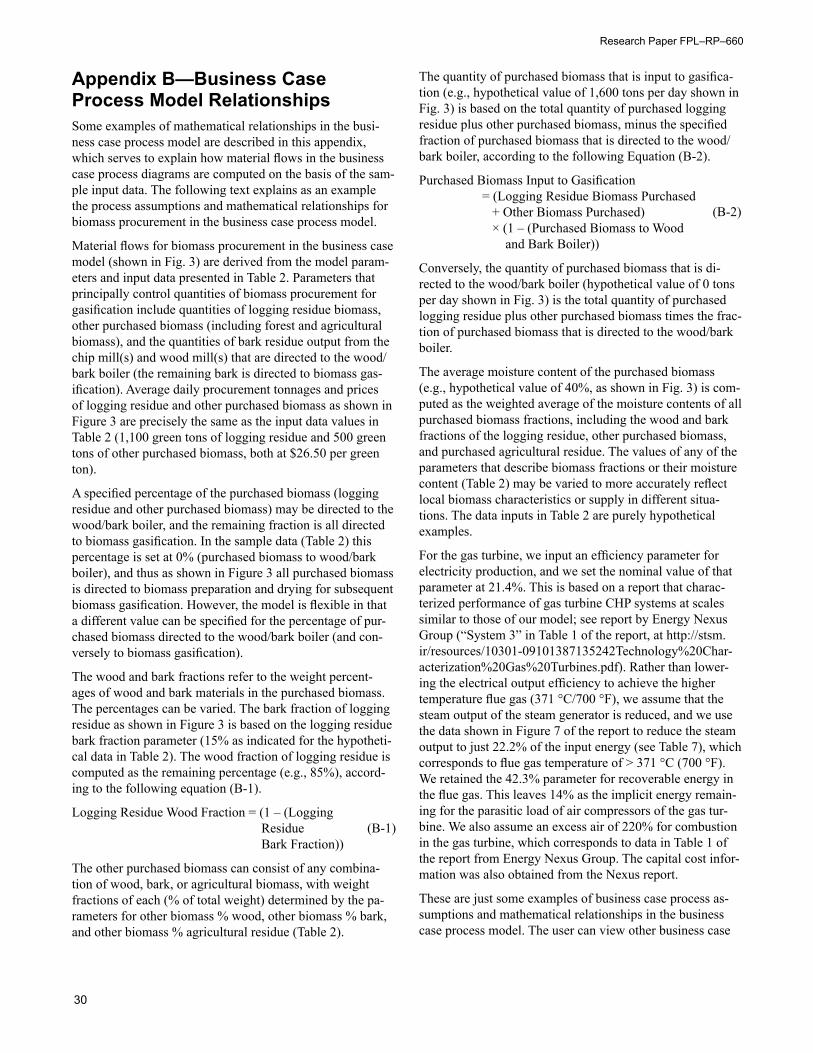
Research Paper FPL–RP–660
30
Appendix B—Business Case Process Model RelationshipsSome examples of mathematical relationships in the busi-ness case process model are described in this appendix, which serves to explain how material flows in the business case process diagrams are computed on the basis of the sam-ple input data. The following text explains as an example the process assumptions and mathematical relationships for biomass procurement in the business case process model.
Material flows for biomass procurement in the business case model (shown in Fig. 3) are derived from the model param-eters and input data presented in Table 2. Parameters that principally control quantities of biomass procurement for gasification include quantities of logging residue biomass, other purchased biomass (including forest and agricultural biomass), and the quantities of bark residue output from the chip mill(s) and wood mill(s) that are directed to the wood/bark boiler (the remaining bark is directed to biomass gas-ification). Average daily procurement tonnages and prices of logging residue and other purchased biomass as shown in Figure 3 are precisely the same as the input data values in Table 2 (1,100 green tons of logging residue and 500 green tons of other purchased biomass, both at $26.50 per green ton).
A specified percentage of the purchased biomass (logging residue and other purchased biomass) may be directed to the wood/bark boiler, and the remaining fraction is all directed to biomass gasification. In the sample data (Table 2) this percentage is set at 0% (purchased biomass to wood/bark boiler), and thus as shown in Figure 3 all purchased biomass is directed to biomass preparation and drying for subsequent biomass gasification. However, the model is flexible in that a different value can be specified for the percentage of pur-chased biomass directed to the wood/bark boiler (and con-versely to biomass gasification).
The wood and bark fractions refer to the weight percent-ages of wood and bark materials in the purchased biomass. The percentages can be varied. The bark fraction of logging residue as shown in Figure 3 is based on the logging residue bark fraction parameter (15% as indicated for the hypotheti-cal data in Table 2). The wood fraction of logging residue is computed as the remaining percentage (e.g., 85%), accord-ing to the following equation (B-1).
Logging Residue Wood Fraction = (1 – (Logging Residue Bark Fraction))
The other purchased biomass can consist of any combina-tion of wood, bark, or agricultural biomass, with weight fractions of each (% of total weight) determined by the pa-rameters for other biomass % wood, other biomass % bark, and other biomass % agricultural residue (Table 2).
The quantity of purchased biomass that is input to gasifica-tion (e.g., hypothetical value of 1,600 tons per day shown in Fig. 3) is based on the total quantity of purchased logging residue plus other purchased biomass, minus the specified fraction of purchased biomass that is directed to the wood/bark boiler, according to the following Equation (B-2).
Purchased Biomass Input to Gasification = (Logging Residue Biomass Purchased + Other Biomass Purchased) × (1 – (Purchased Biomass to Wood and Bark Boiler))
Conversely, the quantity of purchased biomass that is di-rected to the wood/bark boiler (hypothetical value of 0 tons per day shown in Fig. 3) is the total quantity of purchased logging residue plus other purchased biomass times the frac-tion of purchased biomass that is directed to the wood/bark boiler.
The average moisture content of the purchased biomass (e.g., hypothetical value of 40%, as shown in Fig. 3) is com-puted as the weighted average of the moisture contents of all purchased biomass fractions, including the wood and bark fractions of the logging residue, other purchased biomass, and purchased agricultural residue. The values of any of the parameters that describe biomass fractions or their moisture content (Table 2) may be varied to more accurately reflect local biomass characteristics or supply in different situa-tions. The data inputs in Table 2 are purely hypothetical examples.
For the gas turbine, we input an efficiency parameter for electricity production, and we set the nominal value of that parameter at 21.4%. This is based on a report that charac-terized performance of gas turbine CHP systems at scales similar to those of our model; see report by Energy Nexus Group (“System 3” in Table 1 of the report, at http://stsm.ir/resources/10301-09101387135242Technology%20Char-acterization%20Gas%20Turbines.pdf). Rather than lower-ing the electrical output efficiency to achieve the higher temperature flue gas (371 °C/700 °F), we assume that the steam output of the steam generator is reduced, and we use the data shown in Figure 7 of the report to reduce the steam output to just 22.2% of the input energy (see Table 7), which corresponds to flue gas temperature of > 371 °C (700 °F). We retained the 42.3% parameter for recoverable energy in the flue gas. This leaves 14% as the implicit energy remain-ing for the parasitic load of air compressors of the gas tur-bine. We also assume an excess air of 220% for combustion in the gas turbine, which corresponds to data in Table 1 of the report from Energy Nexus Group. The capital cost infor-mation was also obtained from the Nexus report.
These are just some examples of business case process as-sumptions and mathematical relationships in the business case process model. The user can view other business case
(B-1)
(B-2)

Modeling Integrated Biomass Gasification Business Concepts
31
process relationships and formulas in the Excel workbook or contact co-author Mark Dietenberger for additional expla-nation of process model relationships (Mark was primarily responsible for the process model relationships).
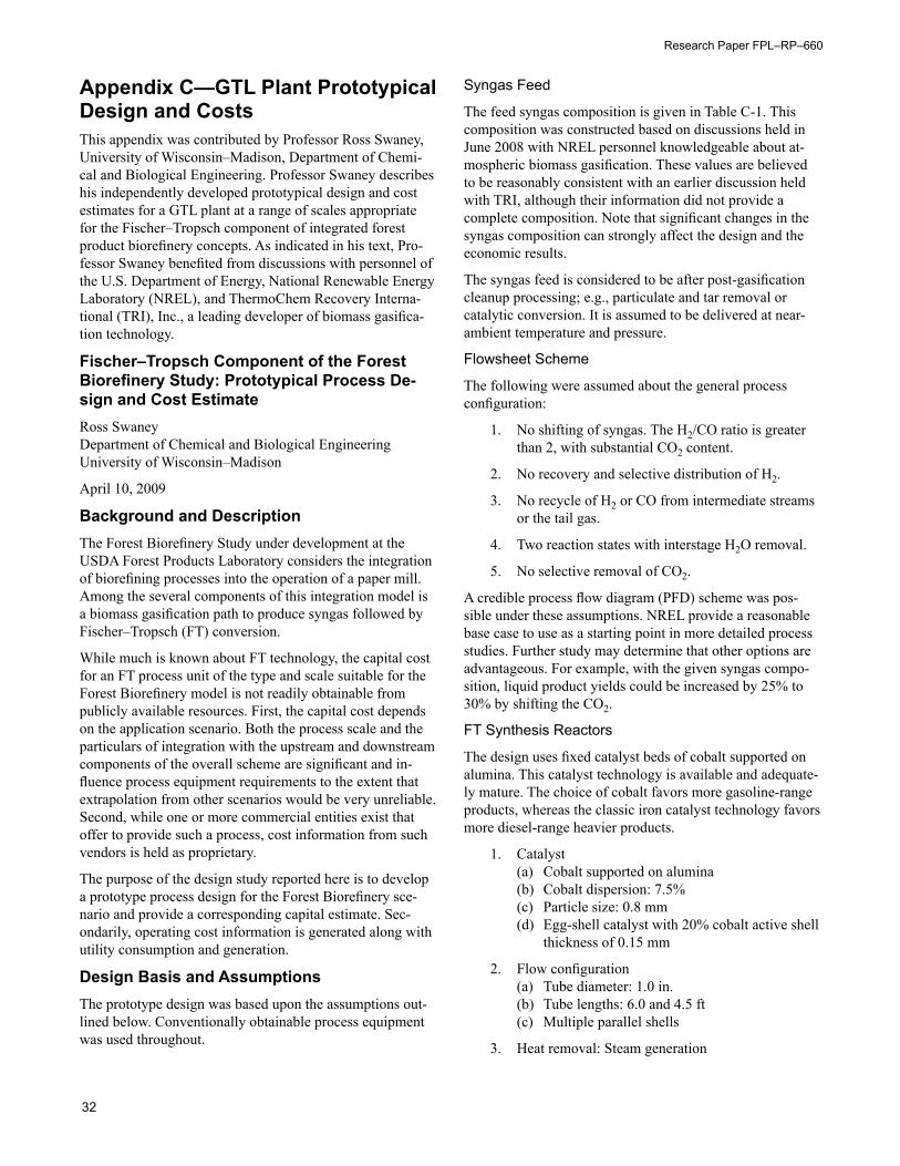
Research Paper FPL–RP–660
32
Appendix C—GTL Plant Prototypical Design and CostsThis appendix was contributed by Professor Ross Swaney, University of Wisconsin–Madison, Department of Chemi-cal and Biological Engineering. Professor Swaney describes his independently developed prototypical design and cost estimates for a GTL plant at a range of scales appropriate for the Fischer–Tropsch component of integrated forest product biorefinery concepts. As indicated in his text, Pro-fessor Swaney benefited from discussions with personnel of the U.S. Department of Energy, National Renewable Energy Laboratory (NREL), and ThermoChem Recovery Interna-tional (TRI), Inc., a leading developer of biomass gasifica-tion technology.
Fischer–Tropsch Component of the Forest Biorefinery Study: Prototypical Process De-sign and Cost EstimateRoss SwaneyDepartment of Chemical and Biological EngineeringUniversity of Wisconsin–Madison
April 10, 2009
Background and DescriptionThe Forest Biorefinery Study under development at the USDA Forest Products Laboratory considers the integration of biorefining processes into the operation of a paper mill. Among the several components of this integration model is a biomass gasification path to produce syngas followed by Fischer–Tropsch (FT) conversion.
While much is known about FT technology, the capital cost for an FT process unit of the type and scale suitable for the Forest Biorefinery model is not readily obtainable from publicly available resources. First, the capital cost depends on the application scenario. Both the process scale and the particulars of integration with the upstream and downstream components of the overall scheme are significant and in-fluence process equipment requirements to the extent that extrapolation from other scenarios would be very unreliable. Second, while one or more commercial entities exist that offer to provide such a process, cost information from such vendors is held as proprietary.
The purpose of the design study reported here is to develop a prototype process design for the Forest Biorefinery sce-nario and provide a corresponding capital estimate. Sec-ondarily, operating cost information is generated along with utility consumption and generation.
Design Basis and AssumptionsThe prototype design was based upon the assumptions out-lined below. Conventionally obtainable process equipment was used throughout.
Syngas Feed
The feed syngas composition is given in Table C-1. This composition was constructed based on discussions held in June 2008 with NREL personnel knowledgeable about at-mospheric biomass gasification. These values are believed to be reasonably consistent with an earlier discussion held with TRI, although their information did not provide a complete composition. Note that significant changes in the syngas composition can strongly affect the design and the economic results.
The syngas feed is considered to be after post-gasification cleanup processing; e.g., particulate and tar removal or catalytic conversion. It is assumed to be delivered at near-ambient temperature and pressure.
Flowsheet Scheme
The following were assumed about the general process configuration:
1. No shifting of syngas. The H2/CO ratio is greater than 2, with substantial CO2 content.
2. No recovery and selective distribution of H2.
3. No recycle of H2 or CO from intermediate streams or the tail gas.
4. Two reaction states with interstage H2O removal.
5. No selective removal of CO2.
A credible process flow diagram (PFD) scheme was pos-sible under these assumptions. NREL provide a reasonable base case to use as a starting point in more detailed process studies. Further study may determine that other options are advantageous. For example, with the given syngas compo-sition, liquid product yields could be increased by 25% to 30% by shifting the CO2.
FT Synthesis Reactors
The design uses fixed catalyst beds of cobalt supported on alumina. This catalyst technology is available and adequate-ly mature. The choice of cobalt favors more gasoline-range products, whereas the classic iron catalyst technology favors more diesel-range heavier products.
1. Catalyst(a) Cobalt supported on alumina(b) Cobalt dispersion: 7.5%(c) Particle size: 0.8 mm(d) Egg-shell catalyst with 20% cobalt active shell
thickness of 0.15 mm
2. Flow configuration(a) Tube diameter: 1.0 in.(b) Tube lengths: 6.0 and 4.5 ft(c) Multiple parallel shells
3. Heat removal: Steam generation
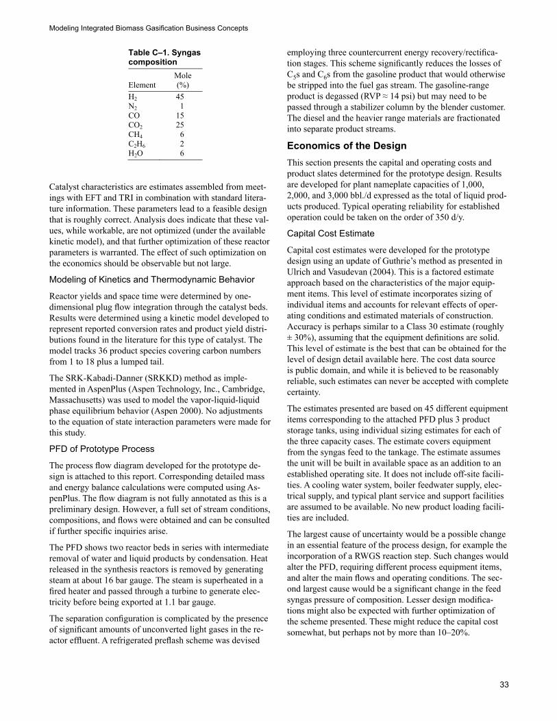
Modeling Integrated Biomass Gasification Business Concepts
33
Catalyst characteristics are estimates assembled from meet-ings with EFT and TRI in combination with standard litera-ture information. These parameters lead to a feasible design that is roughly correct. Analysis does indicate that these val-ues, while workable, are not optimized (under the available kinetic model), and that further optimization of these reactor parameters is warranted. The effect of such optimization on the economics should be observable but not large.
Modeling of Kinetics and Thermodynamic Behavior
Reactor yields and space time were determined by one-dimensional plug flow integration through the catalyst beds. Results were determined using a kinetic model developed to represent reported conversion rates and product yield distri-butions found in the literature for this type of catalyst. The model tracks 36 product species covering carbon numbers from 1 to 18 plus a lumped tail.
The SRK-Kabadi-Danner (SRKKD) method as imple-mented in AspenPlus (Aspen Technology, Inc., Cambridge, Massachusetts) was used to model the vapor-liquid-liquid phase equilibrium behavior (Aspen 2000). No adjustments to the equation of state interaction parameters were made for this study.
PFD of Prototype Process
The process flow diagram developed for the prototype de-sign is attached to this report. Corresponding detailed mass and energy balance calculations were computed using As-penPlus. The flow diagram is not fully annotated as this is a preliminary design. However, a full set of stream conditions, compositions, and flows were obtained and can be consulted if further specific inquiries arise.
The PFD shows two reactor beds in series with intermediate removal of water and liquid products by condensation. Heat released in the synthesis reactors is removed by generating steam at about 16 bar gauge. The steam is superheated in a fired heater and passed through a turbine to generate elec-tricity before being exported at 1.1 bar gauge.
The separation configuration is complicated by the presence of significant amounts of unconverted light gases in the re-actor effluent. A refrigerated preflash scheme was devised
employing three countercurrent energy recovery/rectifica-tion stages. This scheme significantly reduces the losses of C5s and C6s from the gasoline product that would otherwise be stripped into the fuel gas stream. The gasoline-range product is degassed (RVP ≈ 14 psi) but may need to be passed through a stabilizer column by the blender customer. The diesel and the heavier range materials are fractionated into separate product streams.
Economics of the DesignThis section presents the capital and operating costs and product slates determined for the prototype design. Results are developed for plant nameplate capacities of 1,000, 2,000, and 3,000 bbl./d expressed as the total of liquid prod-ucts produced. Typical operating reliability for established operation could be taken on the order of 350 d/y.
Capital Cost Estimate
Capital cost estimates were developed for the prototype design using an update of Guthrie’s method as presented in Ulrich and Vasudevan (2004). This is a factored estimate approach based on the characteristics of the major equip-ment items. This level of estimate incorporates sizing of individual items and accounts for relevant effects of oper-ating conditions and estimated materials of construction. Accuracy is perhaps similar to a Class 30 estimate (roughly ± 30%), assuming that the equipment definitions are solid. This level of estimate is the best that can be obtained for the level of design detail available here. The cost data source is public domain, and while it is believed to be reasonably reliable, such estimates can never be accepted with complete certainty.
The estimates presented are based on 45 different equipment items corresponding to the attached PFD plus 3 product storage tanks, using individual sizing estimates for each of the three capacity cases. The estimate covers equipment from the syngas feed to the tankage. The estimate assumes the unit will be built in available space as an addition to an established operating site. It does not include off-site facili-ties. A cooling water system, boiler feedwater supply, elec-trical supply, and typical plant service and support facilities are assumed to be available. No new product loading facili-ties are included.
The largest cause of uncertainty would be a possible change in an essential feature of the process design, for example the incorporation of a RWGS reaction step. Such changes would alter the PFD, requiring different process equipment items, and alter the main flows and operating conditions. The sec-ond largest cause would be a significant change in the feed syngas pressure of composition. Lesser design modifica-tions might also be expected with further optimization of the scheme presented. These might reduce the capital cost somewhat, but perhaps not by more than 10–20%.
Table C–1. Syngas composition
ElementMole (%)
H2 45N2 1CO 15 CO2 25CH4 6C2H6 2 H2O 6
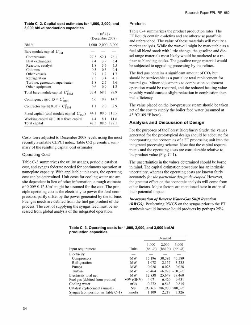
Research Paper FPL–RP–660
34
Costs were adjusted to December 2008 levels using the most recently available CEPCI index. Table C-2 presents a sum-mary of the resulting capital cost estimates.
Operating Cost
Table C-3 summarizes the utility usages, periodic catalyst cost, and syngas federate needed for continuous operation at nameplate capacity. With applicable unit costs, the operating cost can be determined. Unit costs for cooling water use are site dependent in lieu of other information, a rough estimate of 0.009-0.12 $/m3 might be assumed for the cost. The prin-ciple operating cost is the electricity to power the feed com-pressors, partly offset by the power generated by the turbine. Fuel gas needs are debited from the fuel gas product of the process. The cost of supplying the syngas feed must be as-sessed from global analysis of the integrated operation.
Products
Table C-4 summarizes the product production rates. The FT liquids contain α-olefins and are otherwise paraffinic and unbranched. The value of these materials will require a market analysis. While the wax-oil might be marketable as a fuel oil blend stock with little change, the gasoline and die-sel range materials most likely would be marketed to a re-finer as blending stocks. The gasoline range material would be subjected to upgrading processing by the refiner.
The fuel gas contains a significant amount of CO2 but should be serviceable as a partial or total replacement for natural gas. Minor adjustments to combustion equipment operation would be required, and the reduced heating value possibly would cause a slight reduction in combustion ther-mal efficiency.
The value placed on the low-pressure steam should be taken net of the cost to supply the boiler feed water (assumed at 43 °C/109 °F here).
Analysis and Discussion of DesignFor the purposes of the Forest Biorefinery Study, the values generated for the prototypical design should be adequate for incorporating the economics of a FT processing unit into the integrated processing scheme. Note that the capital require-ments and the operating costs are considerable relative to the product value (Fig. C–1).
The uncertainties in the values determined should be borne in mind. The capital estimation procedure has an intrinsic uncertainty, whereas the operating costs are known fairly accurately for the particular design developed. However, the greatest effect on the economic analysis will come from other factors. Major factors are mentioned here in order of their potential impact:
Incorporation of Reverse Water-Gas Shift Reaction (RWGS). Performing RWGS on the syngas prior to the FT synthesis would increase liquid products by perhaps 25%
Table C–2. Capital cost estimates for 1,000, 2,000, and 3,000 bbl./d production capacities
×106 ($) (December 2008)
Bbl./d 1,000 2,000 3,000
Bare module capital aCBM — — — Compressors 27.3 52.1 76.1 Heat exchangers 2.4 3.9 5.4 Reactors, catalyst 1.8 3.6 5.5 Columns 0.3 0.3 0.4 Other vessels 0.7 1.2 1.7 Refrigeration 2.5 3.4 4.1 Turbine, generator, superheater 1.8 2.7 3.6 Other equipment 0.6 0.9 1.2
Total bare module capital aCTBM 37.4 68.3 97.9
Contingency @ 0.15 × aCTBM 5.6 10.2 14.7
Contractor fee @ 0.03 × aCTBM 1.1 2.0 2.9
Fixed capital (total module capital TMC ) 44.1 80.6 115.5 Working capital @ 0.10 × fixed capital 4.4 8.1 11.6 Total capital 48.5 88.6 127.1
Table C–3. Operating costs for 1,000, 2,000, and 3,000 bbl./d production capacities
Demand
Input requirement Units 1,000
(bbl./d)2,000
(bbl./d)3,000
(bbl./d) Electricity — — — —
Compressors MW 15.196 30.393 45.589 Refrigeration MW 1.078 2.157 3.235 Pumps MW 0.028 0.028 0.028 Turbine MW –3.464 –6.928 –10.393
Electricity total net MW 12.838 25.649 38.460 Fuel gas (debited from product) MW (GHV) 4.071 6.420 9.631 Cooling water m3/s 0.272 0.543 0.815 Catalyst replacement (annual) $/y 193,465 386,930 580,395 Syngas (composition in Table C–1) kmol/s 1.109 2.217 3.326

Modeling Integrated Biomass Gasification Business Concepts
35
to 30%. While fuel gas output would be decreased, the rela-tively higher economic value of the liquids should justify the modest increase in capital that would be required.
This change would entail integrating another catalytic reac-tor upstream of the FT reactors. Incorporation would neces-sitate redesign of the entire process. The synthesis reactors would become somewhat larger, while the separation flow scheme is likely to change. With significantly less CO2 and unconverted H2 in the separation, refrigeration can possibly be avoided with attendant savings in capital and operating costs.
The present results strongly indicate that this option may be preferred over the basic design developed here and should be investigated in future work.
Changes in Syngas Composition or Delivery Pressure and Temperature. The nature of the upstream gasifier greatly impacts the economic parameters of the FT process. It is essential to remember that the gasifier and synthesis process must be designed together to work with each other. The design developed and analyzed here is contingent upon the syngas composition and pressure assumed. Changes in the H2/CO/CO2 ratios could substantially affect product yields
Table C–4. Products slates for 1,000, 2,000, and 3,000 bbl./d cases
Product Units
Rate
1,000(bbl./d)
2,000(bbl./d)
3,000 (bbl./d)
FT gasoline stock bbl./d 669.5 1,339.0 2,008.5 FT diesel stock bbl./d 187.1 374.3 561.4 FT wax-oil bbl./d 143.3 286.7 430.0 Fuel gas (net of process usage) MW (GHV) 9.119 18.237 27.356 mol/s 400.6 801.1 1,201.7 Steam @ 2.1 bar, 125 °C kg/s 12.460 24.920 37.380 (FW supplied at no cost) — — — —
Figure C–1. Process flow diagram for prototypical 1,000 barrel per day Fischer-Tropsch section of integrated forest biorefinery (Dr. Ross Swaney, University of Wisconsin).
Research Paper FPL–RP–660
36
and the process design, as well as the desirability of the RWGS option.
Clearly both capital and operating costs of the FT process are dominated by feed compressors. Use of a high-pressure gasifier, while increasing costs of the gasifier, would greatly reduce the costs of the FT unit. This strong interaction must be considered when examining process options.
Other Factors. Several additional aspects may also have some impact:
(a) As presented, the PFD does not incorporate a power re-cover turbine on the fuel gas. Further analysis may indicate that this option is advantageous, providing a significant electrical power credit. This would probably involve three stages with pre/reheat integrated with E-1 and E-2.
(b) The usability/value of the low-pressure stream and the fuel gas need to be verified. If needed, the stream can be supplied at higher pressure by sacrificing some or all of the power obtained from the turbine.
(c) Newer catalyst fabrications, e.g., monoliths, may reduce reactor costs somewhat.
(d) The physical modeling methods should be further vali-dated and refined if so indicated to the extent that relevant data are available. The kinetic model used does not account for the effects of reactor temperature on the product yield distribution. Also, the catalyst run lifecycle will require a progression of reactor operating conditions and the yield distribution will shift to some degree. The VLLE prediction methods should be further validated.
Further technical studies should address the above. Addi-tionally, the market values of the FT liquids will need to be assessed.