Embed Size (px)
Citation preview

“Modeling, Identification and Control of Aerospace Systems”
Luiz Carlos S. Góes and Euler G. BarbosaInstituto Tecnológico de Aeronáutica
DCTA

Presentation Outline• Electrohydraulic Control of a Flexible Structure
– Bond Graph Approach• Bond Graph Modeling of a Slewing Structure• Comparison with Experimental Results• Conclusions

3

- Bond-Graphs is a graphical multiphysics dynamic modeling method invented by professor Henry M. Paynter in MIT in 1959;
- BG is a graphycal representation of the flow of energy and power independent of the physical domain;
- BG modeling permits the visualization of the energy channels through the physical systems, where this energy is stored and dissipated by irreversible processes;

Elements of the BG Language
1 port Elements- Sources
- Energy Storage Devices
- Energy Dissipators
SE, SF
Cg, IgRg
2 portas Elements - Transformers
- Gyrators
TF
GYElements with two or more ports - Parallel Junction
- Series Junction
0
1
5

System Description
• Air bearing system• Central hub• Flexible structure (Plate)• Torsion bar• Electrohydraulic motor• Position sensor (pot)• Vibration sensors (acc.)

The Electrohydraulic Plant

Bond Graph Model – EH System

The Flexible Structure
• Young’s modulus, AluminiumE = 6,89 . 1010 [N/m]
• Mass density, 2795 [kg/m3]• Length, a = 1,41 [m]• Height, b = 46,85 [cm]• Plate thickness, h= 2,65 [mm]• Moment of inertia of the hub, IH
= 3,5 [kg.m2]

Dynamic Model of the Flexible Appendage
• Hamilton Principle:
• Kinetic Energy:
• Potential Energy:
( ) 00
int =+−∫ dtWVKft
tncδ
∫ ∫ ++=b a
H dxdywxmIK0 0
22 )(21
21
θθ
( )∫ ∫
∂∂
∂−
∂∂
∂∂
−−
∂∂
+∂∂
=b a
dxdyyx
wyw
xw
yw
xwDV
0 0
22
2
2
2
22
2
2
2
2
int 1221 ν

Equation of Motion• Rigid body motion, θ(t)• Elastic displacement,
w(x,y,t)
( )
=+∂∂
+∇
=∂∂
++ ∫ ∫
02
24
0 02
2
θ
τθ
xmtwmwD
dydxtwxmII
b a
PH

System Discretization: Assumed Modes• Total displacement :
• Modal Expansion :
• Euler-Bernoulli functions:pinned-free in the x-direction (bending) andfree-free in the y-direction(torsion)
θxtyxwtyxz += ),,(),,(
∑∑= =
=R
n
S
mnmmynx tyxtyxz
1 1)()()(),,( ηφφ

Modal Equations• Mass Matrix:
• Stiffness Matrix:
• Modal Equation: 0=+ ηη KM
∫ ∫=a b
jqypxij dxdymM0 0
φφ
∫ ∫=a b
jqypxij dxdykK0 0
φφ
mynxj mm φφ=
( )ivmynx
iimy
iinxmy
ivnxj Dk φφφφφφ ++= 2

Modal Forces and Flexible Modes• Controlled moment :
• External efforts :
• Flexible Modes :
∫∫ ∫ ++=+b
mynx
a a
nxmynxqynmFnmnmnm dyTdxyFdxyFkm
0
'0
0 02211 )0()(.)(. φφφφφφηη
++= ∫∫∫∫
b
myivmy
b
myiimy
a
nxiinx
a
nxivnx
Fnm dyadydxdxbDk
0000
2 φφφφφφφφ
)(),,( '0 yTtyxT δ=
)()()()(),,( 222111 yyxxFyyxxFtyxF −−+−−= δδδδ

Bond-Graph Representation of the Flexible Plate

Bond-Graph of the Controlled Flexible Structure with Electro
Hydraulic Actuation

Bond-Graph of an Aerospace Flexible Structure with Hydraulic Actuation
• The BG description of the slewing link is coupled to the low-orderequivalent system for the hydraulic actuation system;
• The colour lines (R,G,B) depict graphically the influence of the controltorque at the hub and the coupling forces and moments between thevarious flexible modes of the system;
• This is a unique way to visualize a complex dynamic system that hasrigid body modes coupled to flexural and torsional energy in thesystem, and the low order graphical description of the electrohydraulic servo-actuation system.
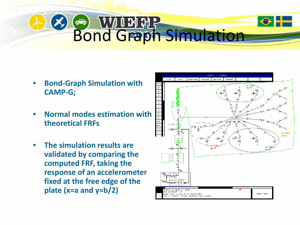
Bond Graph Simulation
• Bond-Graph Simulation with CAMP-G;
• Normal modes estimation with theoretical FRFs
• The simulation results are validated by comparing the computed FRF, taking the response of an accelerometer fixed at the free edge of the plate (x=a and y=b/2)

Modal Response Calculation
Frequency Response Function (FRF) obtained with the linearized model described in the Camp-G environment.

Comparison with Experimental Results
• To validate the BG model, acomparison is madebetween the theoretical-FRFand the experimental-FRFestimated by modal testingas shown in the figure;
• The plate modes wereexcited with a shaker, withthe central hub in a fixedposition.

Experimentally Identified FRF
• Experimental FRFs of the Flexible Plate, accelerometers 5, 6, 7 and 8.

Experimental FRF
• Experimental FRFs of the Fixed Plate, accelerometers9, 10, 11 and 12.

Resonance Frequencies (Hz)
Modal Equations CAMP-G Bond-Graph Model
ExperimentalModal Testing
4,41 4,98 5,015,9 16,0 19,033,2 33,3 33,066,8 66,0 *Out of
Freq.Band73,5 73 *86,1 84 *

Conclusions
• This work presented a BG model of a slewing flexible platecontrolled by a hydraulic servo control system;
• The BG model reproduced the principal characteristics of themulti-domain dynamical system, with the advantage ofproviding a direct visualization of the interaction of principaldynamic effects and its coupling characteristics;
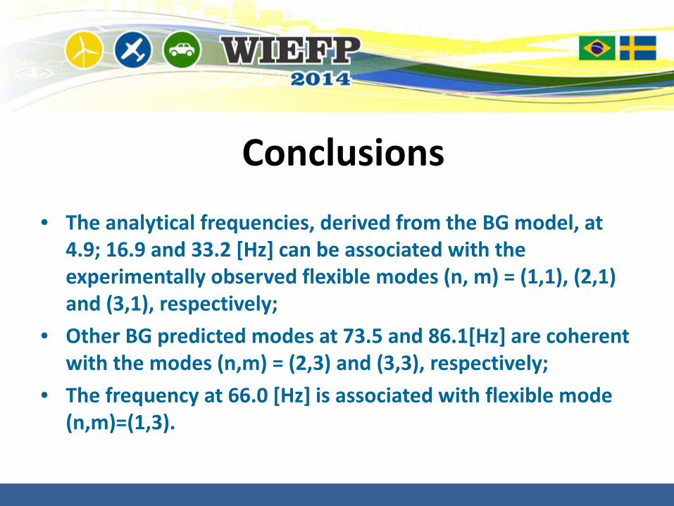
Conclusions• The analytical frequencies, derived from the BG model, at
4.9; 16.9 and 33.2 [Hz] can be associated with the experimentally observed flexible modes (n, m) = (1,1), (2,1) and (3,1), respectively;
• Other BG predicted modes at 73.5 and 86.1[Hz] are coherent with the modes (n,m) = (2,3) and (3,3), respectively;
• The frequency at 66.0 [Hz] is associated with flexible mode (n,m)=(1,3).


![Osprey - Aerospace - Tiger Squadrons [Osprey - Aerospace].pdf](https://img.pdfslide.us/doc/110x75/55cf9675550346d0338b9dbe/osprey-aerospace-tiger-squadrons-osprey-aerospacepdf.jpg)