Modeling Human Behavior in Strategic Settings

by

James Robert Wright

B.Sc., Simon Fraser University, 2000

M.Sc., The University of British Columbia, 2010

A DISSERTATIONSUBMITTED IN PARTIAL FULFILLMENT OF THE

REQUIREMENTS FOR THE DEGREE OF

Doctor of Philosophy

in

THE FACULTY OF GRADUATE AND POSTDOCTORALSTUDIES

(Computer Science)

The University of British Columbia(Vancouver)

August 2016

c© James Robert Wright, 2016

Abstract

Increasingly, electronic interactions between individuals are mediated by special-ized algorithms. One might hope to optimize the relevant algorithms for variousobjectives. An aspect of online platforms that complicates such optimization isthat the interactions are often strategic: many agents are involved, all with theirown distinct goals and priorities, and the outcomes for each agent depend both ontheir own actions, and upon the actions of the other agents.

My thesis is that human behavior can be predicted effectively in a widerange of strategic settings by a single model that synthesizes known devia-tions from economic rationality. In particular, I claim that such a model canpredict human behavior better than the standard economic models. Economicmechanisms are currently designed under behavioral assumptions (i.e., full ratio-nality) that are known to be unrealistic. A mechanism designed based on a moreaccurate model of behavior will be more able to achieve its goal.

In the first part of the dissertation, we develop increasingly sophisticated data-driven models to predict human behavior in strategic settings. We begin by ap-plying machine learning techniques to compare many existing models from be-havioral game theory on a large body of experimental data. We then construct anew family of models called quantal cognitive hierarchy (QCH), which have evenbetter predictive performance than the best of the existing models. We extendthis model with a richer notion of nonstrategic behavior that takes into accountfeatures such as fairness, optimism, and pessimism, yielding further performanceimprovements. Finally, we perform some initial explorations into applying tech-

ii

niques from deep learning in order to automatically learn features of strategicsettings that influence human behavior.

A major motivation for modeling human strategic behavior is to improve thedesign of practical mechanisms for real-life settings. In the second part of thedissertation, we study an applied strategic setting (peer grading), beginning withan analysis of the question of how to optimally apply teaching assistant resourcesto incentivize students to grade each others’ work accurately. We then reportempirical results from using a variant of this system in a real-life undergraduateclass.

iii

Preface

The research described in this dissertation was performed in collaboration withother researchers.

Chapter 2 was co-authored with Kevin Leyton-Brown. An early version waspublished at the Conference of the Association for the Advancement of ArtificialIntelligence [Wright and Leyton-Brown, 2010]. I did the data collection, softwareimplementation, literature review, and wrote the majority of the paper. Kevinprovided guidance throughout, and contributed a significant amount of writingand editing. The methodology, much of the analysis, and all of the figures in thischapter have been updated since publication.

Chapters 3 and 4 were co-authored with Kevin Leyton-Brown. Early ver-sions of portions of the two chapters were published together in the InternationalConference on Autonomous Agents and Multiagent Systems [Wright and Leyton-Brown, 2012]. An updated version was submitted to a journal, and is currentlyunder revision. I did the software implementation and experimental evaluation,and wrote the majority of the paper. Kevin provided guidance and helped writethe text.

Chapter 5 was co-authored with Kevin Leyton-Brown. An early version waspublished in the ACM Conference on Economics and Computation [Wright andLeyton-Brown, 2014]. Kevin and I worked together to design the various alter-native model specifications. I did the software implementation and experimentalevaluation, and wrote the majority of the paper. Kevin provided guidance andhelped write the text. This chapter has been heavily updated since publication.

iv

Chapter 6 was co-authored with Kevin Leyton-Brown and Jason Hartford; it isas-yet unpublished. Jason, Kevin, and I worked together to devise the architecturedescribed in the chapter. I did some early software implementation, but Jason didthe bulk of the implementation. Jason wrote most of the text; I provided guidanceand helped with the text throughout. Kevin also provided guidance and helpedwrite the text.

Chapter 7 was co-authored with Xi Alice Gao and Kevin Leyton-Brown; it isas-yet unpublished. Alice, Kevin, and I worked together to devise the model thatwe evaluate in the chapter. Alice and I worked together on all the proofs. The textin Section 7.3 is primarily due to me; Alice wrote most of the remaining text, withhelp from me. Kevin also provided guidance and helped write the text.

Chapter 8 was co-authored with Kevin Leyton-Brown and Chris Thornton.Jessica Dawson also provided very valuable help with the literature review. Anearly version was published at the ACM Technical Symposium on Computer Sci-ence Education [Wright et al., 2015]. Kevin, Chris, and I worked together todevise the mechanism. Chris did the early implementation of the software de-scribed, and I added the later enhancements described in the chapter. I wrote themajority of the paper. Kevin provided guidance and helped write the paper.

v

Table of Contents

Abstract . . . . . . . . . . . . . . . . . . . . . . . . . . . . . . . . . . . . ii

Preface . . . . . . . . . . . . . . . . . . . . . . . . . . . . . . . . . . . . iv

Table of Contents . . . . . . . . . . . . . . . . . . . . . . . . . . . . . . vi

List of Tables . . . . . . . . . . . . . . . . . . . . . . . . . . . . . . . . . xi

List of Figures . . . . . . . . . . . . . . . . . . . . . . . . . . . . . . . . xii

List of Abbreviations . . . . . . . . . . . . . . . . . . . . . . . . . . . . xiv

Acknowledgments . . . . . . . . . . . . . . . . . . . . . . . . . . . . . . xvi

Dedication . . . . . . . . . . . . . . . . . . . . . . . . . . . . . . . . . . xviii

1 Introduction . . . . . . . . . . . . . . . . . . . . . . . . . . . . . . . 11.1 Behavioral Game Theory as a Machine Learning Problem . . . . . 41.2 Application Domain: Peer Grading . . . . . . . . . . . . . . . . . 61.3 The Way Forward . . . . . . . . . . . . . . . . . . . . . . . . . . 7

vi

I Behavioral Game Theory as a Machine Learning Prob-lem . . . . . . . . . . . . . . . . . . . . . . . . . . . . . . . 8

2 Prediction Performance of Behavioral Game Theoretic Models . . . 92.1 Introduction . . . . . . . . . . . . . . . . . . . . . . . . . . . . . 92.2 Models for Predicting Human Play of Simultaneous-Move Games 12

2.2.1 Quantal Response Equilibrium . . . . . . . . . . . . . . . 132.2.2 Level-k . . . . . . . . . . . . . . . . . . . . . . . . . . . 142.2.3 Cognitive Hierarchy . . . . . . . . . . . . . . . . . . . . 152.2.4 Quantal Level-k . . . . . . . . . . . . . . . . . . . . . . . 162.2.5 Noisy Introspection . . . . . . . . . . . . . . . . . . . . . 18

2.3 Comparing Models . . . . . . . . . . . . . . . . . . . . . . . . . 192.3.1 Prediction Framework . . . . . . . . . . . . . . . . . . . 192.3.2 Assessing Generalization Performance . . . . . . . . . . . 21

2.4 Experimental Setup . . . . . . . . . . . . . . . . . . . . . . . . . 222.4.1 Data . . . . . . . . . . . . . . . . . . . . . . . . . . . . . 222.4.2 Comparing to Nash Equilibrium . . . . . . . . . . . . . . 252.4.3 Computational Environment . . . . . . . . . . . . . . . . 26

2.5 Model Comparisons . . . . . . . . . . . . . . . . . . . . . . . . . 272.5.1 Comparing Behavioral Models . . . . . . . . . . . . . . . 272.5.2 Comparing to Nash Equilibrium . . . . . . . . . . . . . . 302.5.3 Dataset Composition . . . . . . . . . . . . . . . . . . . . 32

2.6 Related Work . . . . . . . . . . . . . . . . . . . . . . . . . . . . 352.7 Conclusions . . . . . . . . . . . . . . . . . . . . . . . . . . . . . 37

3 Parameter Analysis of Behavioral Game Theoretic Models . . . . . 393.1 Introduction . . . . . . . . . . . . . . . . . . . . . . . . . . . . . 393.2 Methods . . . . . . . . . . . . . . . . . . . . . . . . . . . . . . . 41

3.2.1 Posterior Distribution Derivation . . . . . . . . . . . . . . 413.2.2 Posterior Distribution Estimation . . . . . . . . . . . . . . 413.2.3 Visualizing Multi-Dimensional Distributions . . . . . . . 43

vii

3.3 Analysis . . . . . . . . . . . . . . . . . . . . . . . . . . . . . . . 433.3.1 Poisson-CH . . . . . . . . . . . . . . . . . . . . . . . . . 443.3.2 Nash Equilibrium . . . . . . . . . . . . . . . . . . . . . . 463.3.3 QLk . . . . . . . . . . . . . . . . . . . . . . . . . . . . . 46

3.4 Conclusions . . . . . . . . . . . . . . . . . . . . . . . . . . . . . 48

4 Model Variations . . . . . . . . . . . . . . . . . . . . . . . . . . . . . 504.1 Construction . . . . . . . . . . . . . . . . . . . . . . . . . . . . . 504.2 Simplicity Versus Predictive Performance . . . . . . . . . . . . . 524.3 Parameter Analysis . . . . . . . . . . . . . . . . . . . . . . . . . 544.4 Spike-Poisson . . . . . . . . . . . . . . . . . . . . . . . . . . . . 554.5 Conclusions . . . . . . . . . . . . . . . . . . . . . . . . . . . . . 56

5 Models of Level-0 Behavior . . . . . . . . . . . . . . . . . . . . . . . 585.1 Introduction . . . . . . . . . . . . . . . . . . . . . . . . . . . . . 585.2 Level-0 Model . . . . . . . . . . . . . . . . . . . . . . . . . . . . 59

5.2.1 Level-0 Features . . . . . . . . . . . . . . . . . . . . . . 595.2.2 Combining Feature Values . . . . . . . . . . . . . . . . . 645.2.3 Feature Transformations . . . . . . . . . . . . . . . . . . 65

5.3 Model Selection . . . . . . . . . . . . . . . . . . . . . . . . . . . 665.3.1 Forward Selection . . . . . . . . . . . . . . . . . . . . . . 665.3.2 Bayesian Optimization . . . . . . . . . . . . . . . . . . . 675.3.3 Extended Model Performance . . . . . . . . . . . . . . . 695.3.4 Parameter Analysis . . . . . . . . . . . . . . . . . . . . . 71

5.4 Related Work . . . . . . . . . . . . . . . . . . . . . . . . . . . . 755.5 Conclusions . . . . . . . . . . . . . . . . . . . . . . . . . . . . . 76

6 Deep Learning for Human Strategic Modeling . . . . . . . . . . . . 786.1 Introduction . . . . . . . . . . . . . . . . . . . . . . . . . . . . . 786.2 Related Work . . . . . . . . . . . . . . . . . . . . . . . . . . . . 796.3 Modeling Human Strategic Behavior with Deep Networks . . . . 80

viii

6.3.1 Feature Layers . . . . . . . . . . . . . . . . . . . . . . . 826.4 Experimental Setup . . . . . . . . . . . . . . . . . . . . . . . . . 886.5 Experimental Results . . . . . . . . . . . . . . . . . . . . . . . . 896.6 Regular Neural Network Performance . . . . . . . . . . . . . . . 916.7 Conclusions . . . . . . . . . . . . . . . . . . . . . . . . . . . . . 92

II Application Domain: Peer Grading . . . . . . . . . . . 94

7 Incentivizing Evaluation via Limited Access to Ground Truth . . . . 957.1 Introduction . . . . . . . . . . . . . . . . . . . . . . . . . . . . . 967.2 Peer-Prediction Mechanisms . . . . . . . . . . . . . . . . . . . . 997.3 Impossibility of Pareto-Dominant, Truthful Elicitation . . . . . . . 1047.4 Combining Elicitation with Limited Access to Ground Truth . . . 1067.5 When Does Peer-Prediction Help? . . . . . . . . . . . . . . . . . 1087.6 Conclusions . . . . . . . . . . . . . . . . . . . . . . . . . . . . . 1127.7 Proofs . . . . . . . . . . . . . . . . . . . . . . . . . . . . . . . . 114

7.7.1 Proof of Lemma 1 . . . . . . . . . . . . . . . . . . . . . . 1147.7.2 Proof of Lemma 2 . . . . . . . . . . . . . . . . . . . . . . 1157.7.3 Proof of Lemma 3 . . . . . . . . . . . . . . . . . . . . . . 1177.7.4 Proof of Theorem 3 . . . . . . . . . . . . . . . . . . . . . 1187.7.5 Proof of Lemma 4 . . . . . . . . . . . . . . . . . . . . . . 1197.7.6 Proof of Corollary 1 . . . . . . . . . . . . . . . . . . . . . 1217.7.7 Proof of Corollary 2 . . . . . . . . . . . . . . . . . . . . . 125

8 Application: Mechanical TA . . . . . . . . . . . . . . . . . . . . . . 1298.1 Introduction . . . . . . . . . . . . . . . . . . . . . . . . . . . . . 1298.2 Peer Evaluation Model . . . . . . . . . . . . . . . . . . . . . . . 132

8.2.1 Supervised and Independent Reviewers . . . . . . . . . . 1338.2.2 Calibration . . . . . . . . . . . . . . . . . . . . . . . . . 133

8.3 Evolution of our Design . . . . . . . . . . . . . . . . . . . . . . . 1348.3.1 Calibration Setup . . . . . . . . . . . . . . . . . . . . . . 135

ix

8.3.2 Independent Reviewers . . . . . . . . . . . . . . . . . . . 1358.3.3 Exam Performance . . . . . . . . . . . . . . . . . . . . . 137

8.4 Analysis of our Current Design . . . . . . . . . . . . . . . . . . . 1388.4.1 Review Quality . . . . . . . . . . . . . . . . . . . . . . . 1388.4.2 Calibration Performance . . . . . . . . . . . . . . . . . . 140

8.5 Related Work . . . . . . . . . . . . . . . . . . . . . . . . . . . . 1428.6 Conclusions . . . . . . . . . . . . . . . . . . . . . . . . . . . . . 144

Bibliography . . . . . . . . . . . . . . . . . . . . . . . . . . . . . . . . . 146

A CPSC 430 2014 grading rubric . . . . . . . . . . . . . . . . . . . . . 160

x

List of Tables

Table 2.1 Names and contents of each dataset. . . . . . . . . . . . . . . . 25Table 2.2 Previous estimates of level-0 proportions . . . . . . . . . . . . 29Table 2.3 Datasets conditioned on various game features . . . . . . . . . 33Table 2.4 Existing work in model comparison . . . . . . . . . . . . . . . 38

Table 4.1 Model variations with prediction performance . . . . . . . . . 51

xi

List of Figures

Figure 2.1 Likelihoods of model predictions . . . . . . . . . . . . . . . . 28Figure 2.2 Likelihoods on “treasure” and “contradiction” treatments . . . 31Figure 2.3 Likelihoods on feature-based datasets . . . . . . . . . . . . . 35

Figure 3.1 Cumulative posterior distributions for Poisson-CH . . . . . . 44Figure 3.2 Distributions for Poisson-CH and QRE by dominance-solvability 45Figure 3.3 Posterior distributions for NEE . . . . . . . . . . . . . . . . . 47Figure 3.4 Posterior distributions for QLk on ALL10 . . . . . . . . . . . 48

Figure 4.1 Model simplicity vs. prediction performance . . . . . . . . . . 52Figure 4.2 Posterior precision distributions for ah-QCH3 and ah-QCH4 . . 53Figure 4.3 Posterior distributions for ah-QCH3 and ah-QCH4 . . . . . . . 54Figure 4.4 Model simplicity vs. prediction performance for efficient mod-

els, QLk, and Spike-Poisson QCH . . . . . . . . . . . . . . . 57

Figure 5.1 Prediction performance with binary features . . . . . . . . . . 67Figure 5.2 Training and test performance with binary features . . . . . . 68Figure 5.3 Prediction performance for Bayesian optimization incumbents 69Figure 5.4 Prediction performance for Poisson-CH, Lk, and Spike-Poisson

QCH with linear8, linear4, and uniform level-0 specifi-cations. . . . . . . . . . . . . . . . . . . . . . . . . . . . . . 70

Figure 5.5 Posterior distributions of levels for linear4, linear8, anduniform . . . . . . . . . . . . . . . . . . . . . . . . . . . . . 71

xii

Figure 5.6 Posterior precision distributions for linear8, linear4, anduniform . . . . . . . . . . . . . . . . . . . . . . . . . . . . . 72

Figure 5.7 Posterior distribution of weights for linear4 . . . . . . . . . 73Figure 5.8 Posterior distribution of weights for linear8 . . . . . . . . . 74

Figure 6.1 A schematic representation of our architecture . . . . . . . . . 82Figure 6.2 Graphical explanation of pooling units . . . . . . . . . . . . . 85Figure 6.3 Prediction performance for GameNet vs. QCH, varying num-

ber of hidden units and layers. . . . . . . . . . . . . . . . . . 89Figure 6.4 Prediction performance for GameNet vs. QCH, no pooling units. 90Figure 6.5 Prediction performance for GameNet vs. QCH, varying num-

ber action response layers. . . . . . . . . . . . . . . . . . . . 91Figure 6.6 Prediction performance of a feed forward neural network on

fixed-size games with and without data augmentation . . . . . 92

Figure 8.1 Proportion of independent reviewers . . . . . . . . . . . . . . 136Figure 8.2 Distributions of final and midterm exam marks . . . . . . . . 137Figure 8.3 Mean review quality distributions . . . . . . . . . . . . . . . 141Figure 8.4 Deviations from gold standard reviews on calibrations vs. num-

ber of calibrations after promotion . . . . . . . . . . . . . . . 142

xiii

List of Abbreviations

BGT Behavioral Game Theory

BTS Bayesian Truth Serum

CDF cumulative density function

CH cognitive hierarchy

CMA-ES Covariance Matrix Adaptation Evolution Strategy

CPR Calibrated Peer Review

Lk level-k

MAP Maximum a Posteriori

MCMC Markov Chain Monte Carlo

MLE maximum likelihood estimation

MLP multi-layer perceptron

NEE Nash Equilibrium with Error

NI noisy introspection

QCH quantal cognitive hierarchy

QLk quantal level-k

xiv

QRE quantal response equilibrium

TA teaching assistant

xv

Acknowledgments

Many people deserve recognition for their contributions to this work.First and foremost, I would like to thank my advisor Kevin Leyton-Brown. It

is impossible to overstate the importance of his guidance. He has a rare talentfor getting right to the crux of the matter, and has saved me from so many blindalleys that I cannot count them. He has taught me more about the presentationof ideas and the workings of the research world than anyone I know. Kevin hasbeen incredibly generous. He has gone to considerable effort to secure amazingopportunities for me, as well as the financial support to make them feasible andthe guidance to ensure that I made the most of them. Grad school was a wonderfulexperience for me, and having Kevin as an advisor was a major reason why.

Over the years, the Game Theory and Decision Theory reading group wasalways one of my favorite parts of the week. I could always count on insightfuldiscussions, whether research-related or not. I am indebted to my collaboratorsand co-authors, especially Alice Gao and Jason Hartford. I have learned a greatdeal by working with them.

I am grateful to my supervisory committee members, Yoram Halevy and Hol-ger Hoos, for their guidance. Before he was on my committee, Yoram’s class onbehavioral economics early in my degree was of critical value. I am also gratefulto many others in the research community for their help and influence. I wouldparticularly like to mention Colin Camerer, Kate Larson, and David Parkes.

Finally, none of this would have been possible without the patience and sup-port of my family, especially Sarah. She has been unfailingly supportive in more

xvi

ways than I can name.This work was funded in part by a Canada Graduate Scholarship from the Nat-

ural Sciences and Engineering Research Council of Canada, a Four Year Fellow-ship from the University of British Columbia, and a Collaborative Research andDevelopment Grant funded by the Natural Sciences and Engineering ResearchCouncil of Canada and Google Inc. This work was completed in part while I wasvisiting the Simons Institute for the Theory of Computing.

xvii

For Sarah, Miles, and Edith

xviii

Chapter 1

Introduction

Increasingly, electronic interactions between individuals are mediated by special-ized algorithms. For example, someone seeking short term accommodation mightpreviously have searched free-form text ads on craigslist, whereas now a site suchas Airbnb provides specific procedures for finding, booking, and paying for ac-commodations. Other platforms facilitate interactions that were not previouslypractical online, such as Uber and Lyft’s matching of drivers to passengers, or theuse of peer grading in large online courses.

All of these interactions generate data. One might hope to use this data tooptimize the relevant algorithms in terms of various objectives. Indeed, manyplatforms use A/B testing for just such a purpose, using a modified algorithm fora random sample of their users and the original algorithm for the rest, and com-paring the outcomes to determine which performs better. However, A/B testinghas drawbacks. Only a low-dimensional space of variations can realistically beexplored, and along the way many users will potentially be exposed to designsthat are worse than the original.

One aspect of online platforms that makes interaction optimization especiallydifficult is that the interactions are often strategic. A strategic interaction has twomain hallmarks. First, many agents are involved, all with their own distinct goalsand priorities; in the online platform case the agents correspond to the users and

1

the platform designer. Second, the outcomes for each agent depend both on theirown actions, and upon the actions of the other agents. For example, the outcomein an auction depends not only on how the winning bidder bids, but also on howthe losing bidders bid, and on the auction’s rules. Hence in order to act effectivelyin a strategic setting, an agent must reason not only about his own actions, but alsoabout the beliefs and actions of the other agents, who are in turn reasoning aboutall the other agents’ beliefs and action as well. In strategic settings, it can turn outthat straightforward A/B testing does not accurately evaluate either of the optionsunder test [Chawla et al., 2014].

An alternative approach is to learn a model of how people will react to analgorithm. One can then optimize among different designs by evaluating theircounterfactual performance based on the model. This allows the modeler to ex-plore a larger design space at a lower cost. However, such models are rare. Thisdissertation describes a research program that aims to construct a general modelthat can be applied to many strategic settings.

My thesis is that human behavior can be predicted effectively in a widerange of strategic settings by a single model that synthesizes known devia-tions from economic rationality. In particular, I claim that such a model canpredict human behavior better than the standard economic models. Economicmechanisms are currently designed under behavioral assumptions (i.e., full ratio-nality) that are known to be unrealistic. A mechanism designed based on a moreaccurate model of behavior will be more able to achieve its goal, whether thatgoal is social welfare, revenue, or any other aim. This approach of synthesizingmany behavioral anomalies into a single model contrasts with a common approachin economics, where a model is constructed that explains or “rationalizes” a sin-gle anomaly [e.g., Gilboa and Schmeidler, 1989, for ambiguity aversion] or asmall number of anomalies [e.g., Tversky and Kahneman, 1992, for loss aversionand distorted probability judgments], without necessarily evaluating the predictivestrength of the model.

In the rest of the dissertation, we develop data-driven models to predict human

2

strategic behavior; that is, behavior in settings where each participant’s rewardsdepend partially on the actions of other participants. This has important differ-ences from most other machine learning problems. Firstly, each participant’s be-havior is strongly influenced by that of the others, and by their own forecasts ofothers’ behavior. Second, participants’ strategic behavior can be strongly influ-enced by counterfactuals; i.e., what would have happened had they, or other par-ticipants, behaved differently. Furthermore, different algorithm designs often in-volve differences in the set of choices that are available to the participants. Hence,a model used for answering counterfactual questions about alternate designs mustbe able to predict in a setting that has a completely different dimensionality thanthe setting that produced its training data. Thus, prediction in these settings can-not be framed as a classification problem in which one of a fixed set of labels ispredicted. Similarly, the need to generalize between datasets with different di-mensions of both inputs and outputs means that deep learning techniques cannotbe straightforwardly applied in these settings.

Game theory is the standard mathematical framework for understanding strate-gic interactions. Game theoretic models assume that the participants in an in-teraction are idealized, perfectly rational agents. This is clearly an unrealisticassumption for individuals, and indeed, we know from both experimental andobservational data that standard game theoretic models describe human behaviorvery poorly [Goeree and Holt, 2001; Rabin, 2000]. The interdisciplinary field ofbehavioral game theory (BGT) investigates deviations from the standard modelsof game theory, and proposes new models of human behavior by taking accountof human cognitive biases and limitations [Camerer, 2003]. These models canbe understood as parametric functions that can be applied to inputs of arbitrarydimension.

The dissertation is divided into two parts: behavioral game theory as a machinelearning problem, and the peer grading application domain.

3

1.1 Behavioral Game Theory as a MachineLearning Problem

My long-term research agenda is to build a general theory for optimally designingalgorithms that mediate interactions between humans, rather than between ideal-ized agents. The BGT literature has proposed a great many models to describehuman strategic behavior. However, synthesizing them into a usable predictivemodel for algorithm design requires computational tools that are not typicallyavailable to behavioral game theorists. For example, a natural question for a ma-chine learning specialist would be, which of the many BGT models has the bestout-of-sample prediction performance? The standard BGT technique for compar-ing models is to perform statistical tests comparing a general model’s in-sampleperformance to a specialized version; this makes it impossible to compare non-nested models (i.e., models where neither is a strict generalization of the other)and is prone to preferring models that overfit to the training data.

In Chapter 2, we compare the prediction performance of six well known BGTmodels according to the standards of the machine learning community. Usinga large body of experimental data collected from multiple sources in the liter-ature, we performed a cross-validated comparison of the out-of-sample predic-tion performance of the models. This comparison involved computing maximumlikelihood estimates of extremely nonlinear models, which required considerablecomputational expertise and resources, including over one year of CPU time ona high-performance computing cluster. Remarkably, we found that one particularmodel performed better than all of the others in most individual datasets, as wellas in the combined dataset. This model incorporates two crucial elements: first,agents do not choose optimally according to their beliefs. Rather, they quantally

respond, with every action being chosen with positive probability, but more op-timal actions being chosen proportionally more often. Second, it is an iterative

model: each agent is assumed to have a level representing the number of stepsof strategic reasoning that it is capable of. Level-0 agents do not reason aboutthe other agents; level-1 agents believe that all of their opponents are level-0 and

4

respond accordingly; and so forth.One advantage of structural models—models whose parameters have a causal

interpretation—is that the parameter values, if known, can help researchers under-stand reasons and mechanisms behind observed behavior. Thus, good parameterestimates are valuable both for optimizing a model’s prediction performance, andalso for providing scientific insight in their own right. Maximum likelihood esti-mation chooses parameters in a sensible way for comparing model performance,but it is less valuable for providing insight. In Chapter 3, we introduce a Bayesianframework for estimating a behavioral model’s full posterior parameter distribu-tion. We used this framework to analyze several models from Chapter 2, includingthe best-performing one. This produced insights that we build upon in Chapter 4to construct a family of models that is both more parsimonious and more robust,and also predicts the data better, while requiring fewer parameters to be learned.

In any iterative model, agents reason about the behavior of their opponentsstarting from a specification of nonstrategic (level-0) behavior. Despite the pivotalrole that it plays in determining the actions of higher-level agents, modeling level-0 behavior has received virtually no attention in the literature; in practice, almostall existing work specifies this behavior as a uniform distribution over actions.In most games it is not plausible that even nonstrategic agents would choose anaction uniformly at random, nor that other agents would expect them to do so. InChapter 5, we construct a richer model of level-0 behavior that can be plugged intoany iterative model, in which level-0 agents choose actions that are in some waysalient (e.g., by having the maximal best case, or by forming part of the fairestoutcome). This level-0 model dramatically improved the performance of severaliterative models.

The properties of actions that people might find salient—and which mightthus be favored by nonstrategic agents—have thus far been discovered primarilyby asking “How might I reason about playing this specific game?” Rather thanrelying solely on introspection and domain knowledge, we might hope to derivesuch properties directly from data. Deep learning [e.g., Bengio, 2009] has shown

5

success in a wide range of domains for automatically discovering features. InChapter 6, we take the first steps toward adapting deep learning techniques to thestrategic prediction domain with the goal of discovering new representations ofsalient game characteristics.

The invention of the pooling and convolution operators was a major advancein the application of deep neural networks to vision tasks [LeCun et al., 1998].These operators exploit invariances and local structure in the domain to allowfor vastly more efficient training of deep networks. Strategic games have a verydifferent structure. A game is essentially the same game if the action labels arepermuted, which means that local structure is less exploitable. Additionally, dif-ferent games, even in the same domain, can have very different dimensionalitydepending on how many actions are available to each participant and how manyparticipants there are. Intuitively speaking, the approach that we take in Chapter 6aims to devise the equivalent of pooling and convolution operators for strategicmodeling. This direction has proven extremely promising; the model that wepresent already achieves significant improvements in prediction performance overany of the structural models that we study, albeit at the expense of completely sac-rificing interpretability. In future work, we hope to combine the interpretability ofa structural model with the superior prediction performance of a deep model.

1.2 Application Domain: Peer GradingThe first part of the dissertation aims to construct a model that can be applied toany one-shot strategic setting involving human participants. In the second partof the dissertation, we shift from this general approach to focus in on a specificsetting of this kind: peer grading, in which an instructor wishes to incentivizestudents to honestly and diligently evaluate each others’ work.

We begin by performing a theoretical analysis of a more general problem thatincludes peer grading as a special case: eliciting truthful evaluations of arbitraryobjects. There is a large literature on the problem of peer prediction, in whichagents are incentivized to truthfully report their observations of a ground truth to

6

which the mechanism designer has no access whatsoever. The essential contribu-tion of Chapter 7 is to analyze a more realistic setting, in which the mechanismdesigner has access to this ground truth, but only at a cost, which the designerwishes to minimize or avoid entirely. The peer prediction literature relies heavilyon a particular assumption—that agents can coordinate only through the informa-tion that the mechanism wishes to elicit. We first show that when this assumptionis relaxed, agents are almost surely better off not reporting their observations truth-fully. This demonstrates that the assumption is not merely innocuous or technical.Second, we show that in the presence of costly access to ground truth, a simpledominant-strategy mechanism can elicit truthful reports better (in the sense of re-quiring less ground truth) than any of the peer prediction mechanisms of whichwe are aware.

Finally, in Chapter 8, we describe the outcomes of using a variant of thedominant-strategy mechanism from Chapter 7 in a real undergraduate class. Thispeer grading platform eventually formed the cornerstone of the class. The plat-form is now freely available for download, and has since been used at multipleother universities.

1.3 The Way ForwardAs almost every aspect of our lives is increasingly mediated by algorithms, im-proving these algorithms has become increasingly valuable. But such improve-ment requires accurate models of how people will respond to the algorithms, andto each others’ responses. With the growing availability of data, there is now anunprecedented opportunity to understand and predict human strategic behaviorusing a principled machine learning approach. My hope is that this dissertationwill prove to be an important step along the way to achieving this goal.

7

Part I

Behavioral Game Theory as aMachine Learning Problem

8

Chapter 2

Prediction Performance ofBehavioral Game Theoretic Models

2.1 IntroductionIn strategic settings, it is common to assume that agents will adopt Nash equi-librium strategies, behaving so that each optimally responds to the others. Thissolution concept has many appealing properties; e.g., under any other strategyprofile, one or more agents will regret their strategy choices. However, experi-mental evidence shows that Nash equilibrium often fails to describe human strate-gic behavior [see, e.g., Goeree and Holt, 2001]—even among professional gametheorists [Becker et al., 2005].

The relatively new field of behavioral game theory extends game-theoreticmodels to account for human behavior by accounting for human cognitive bi-ases and limitations [Camerer, 2003]. Experimental evidence is the foundationof behavioral game theory, and researchers have developed many models of howhumans behave in strategic situations based on such data. This multitude of mod-els presents a practical problem, however: which model should we use to predicthuman behavior?

Existing work in behavioral game theory does not directly answer this ques-

9

tion, for two reasons. First, it has tended to focus on explaining (fitting) in-samplebehavior rather than predicting out-of-sample behavior. This means that modelsare vulnerable to overfitting the data: the most flexible model can be chosen in-stead of the most accurate one. Second, behavioral game theory has tended notto compare multiple behavioral models, instead either exploring elaborations ofa single model or comparing only to one other model (typically Nash equilib-rium). In this chapter we perform rigorous—albeit computationally intensive—comparisons of many different models and model variations on a wide range ofexperimental data, leading us to believe that ours is the most comprehensive studyof its kind.

Our focus is on the most basic of strategic interactions: unrepeated (initial)play in simultaneous move games. In the behavioral game theory literature, fivekey paradigms have emerged for modeling human decision making in this setting:quantal response equilibrium [QRE; McKelvey and Palfrey, 1995]; the noisy in-trospection model [NI; Goeree and Holt, 2004]; the cognitive hierarchy model[CH; Camerer et al., 2004]; the closely related level-k [Lk; Costa-Gomes et al.,2001; Nagel, 1995] models; and what we dub quantal level-k [QLk; Stahl andWilson, 1994] models. Although there exist studies exploring different variationsof these models [e.g., Stahl and Wilson, 1995; Ho et al., 1998; Weizsacker, 2003;Rogers et al., 2009], the overwhelming majority of behavioral models of initialplay of normal-form games fall broadly into this categorization.

The first contribution of our work is methodological: we demonstrate broadlyapplicable techniques for comparing and analyzing behavioral models. We il-lustrate the use of these techniques via an extensive meta-analysis based on datapublished in ten different studies, rigorously comparing Lk, QLk, CH, NI, andQRE to each other and to a model based on Nash equilibrium. The findings thatresult from this meta-analysis both demonstrate the usefulness of the approachand constitute our second contribution.

All of these models depend upon exogenous parameters. Most previous workhas focused on models’ ability to describe human behavior, and hence has sought

10

parameter values that best explain observed experimental data, or more formallythat maximize a dataset’s probability. (All of the models that we consider makeprobabilistic predictions; thus, we must score models according to how muchprobability mass they assign to observed events, rather than assessing accuracy.)We depart from this descriptive focus, seeking to find models, and hence param-eter values, that are effective for predicting previously unseen human behavior.Thus, we follow a different approach taken from machine learning and statistics.We begin by randomly dividing the experimental data into a training set and a testset. We then set each model’s parameters to values that maximize the likelihoodof the training dataset, and finally score each model according to the (disjoint) testdataset’s likelihood. To reduce the variance of this estimate without biasing itsexpected value, we employ cross-validation [e.g., Bishop, 2006], systematicallyrepeating this procedure with different test and training sets.

Our meta-analysis has led us to draw three qualitative conclusions. First, andleast surprisingly, Nash equilibrium is less able to explain human play than behav-ioral models. Second, two high-level themes that underlie the five behavioral mod-els (which we dub “cost-proportional errors” and “limited iterative strategic think-ing”) appear to model independent and predictively useful phenomena. Third, andbuilding on the previous conclusion, the quantal level-k model of Stahl and Wilson[1994] (QLk)—which combines both of these themes—made the most accuratepredictions. Specifically, QLk substantially outperformed all other models on anew dataset spanning all data in our possession, and also had the best or nearlythe best performance on each individual dataset. Our findings were quite robustto variation in the games played by human subjects. We broke down model per-formance by game properties such as dominance structure and number/types ofequilibria, and obtained essentially the same results as on the combined dataset.We do note that our datasets consisted entirely of two-player games. Previouswork suggests that human subjects reason about n-player games as if they weretwo-player games, failing to fully account for the independence of the other play-ers’ actions [Ho et al., 1998; Costa-Gomes et al., 2009]; we might thus expect to

11

observe qualitatively similar results in the n-player case. Nevertheless, empiri-cally confirming this expectation is an important future direction.

In the next section, we define the models that we study. Section 2.3 lays outthe formal framework within which we work, and Section 2.4 describes our data,methods, and the Nash-equilibrium-based model to which we compare the behav-ioral models. Section 2.5 presents the results of our comparisons. In Section 2.6we survey related work from the literature and explain how our own work con-tributes to it. We conclude in Section 2.7.

2.2 Models for Predicting Human Play ofSimultaneous-Move Games

Formally, a normal-form game G is a tuple (N,A, u), where N is a finite set ofagents; A = ∏

i∈N Ai is the set of possible action profiles; Ai is the finite set ofactions available to agent i; u = {ui}i∈N is a set of utility functions ui : A → R,each of which maps from an action profile to a utility for agent i. Let ∆(X) denotethe set of probability distributions over a finite set X . Overloading notation, werepresent the expected utility of a profile of mixed strategies s ∈ S = ∏

i∈N ∆(Ai)by ui(s). We use the notation a−i to refer to the joint actions of all agents exceptfor i.

A behavioral model is a mapping from a game G and a vector of parametersθ to a predicted distribution over each action profile a ∈ A, which we denotePr(a |G, θ). In what follows, we define five prominent behavioral models of hu-man play in unrepeated, simultaneous-move games.1

1We focus here on models of behavior in general one-shot normal-form games. We omitmodels of learning in repeated normal-form games such as impulse-balance equilibrium [Seltenand Buchta, 1994], payoff-sampling equilibrium [Osborne and Rubinstein, 1998], action-samplingequilibrium [Selten and Chmura, 2008], and experience-weighted attraction [Camerer and Hua Ho,1999], and models restricted to a single game class (e.g., symmetric games) such as cooperativeequilibrium [Capraro, 2013]. We also omit variants and generalizations of the models we study,such as those introduced by Rogers et al. [2009], Weizsacker [2003], and Cabrera et al. [2007];but see Chapter 4, where we systematically explored a particular space of variants.

12

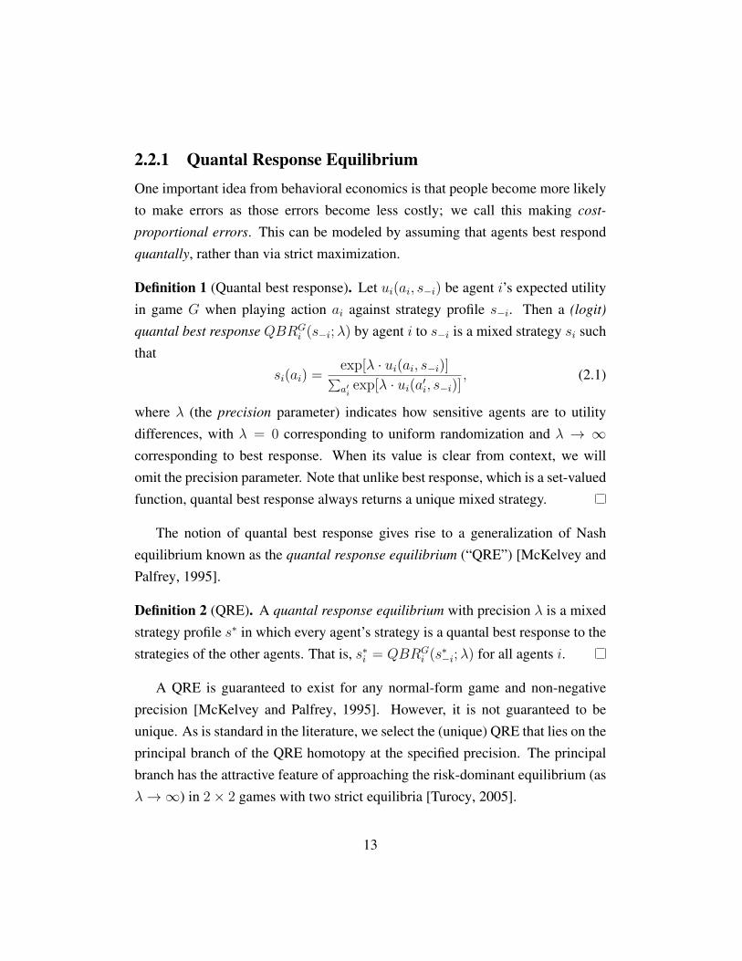
2.2.1 Quantal Response EquilibriumOne important idea from behavioral economics is that people become more likelyto make errors as those errors become less costly; we call this making cost-

proportional errors. This can be modeled by assuming that agents best respondquantally, rather than via strict maximization.

Definition 1 (Quantal best response). Let ui(ai, s−i) be agent i’s expected utilityin game G when playing action ai against strategy profile s−i. Then a (logit)

quantal best response QBRGi (s−i;λ) by agent i to s−i is a mixed strategy si such

thatsi(ai) = exp[λ · ui(ai, s−i)]∑

a′iexp[λ · ui(a′i, s−i)]

, (2.1)

where λ (the precision parameter) indicates how sensitive agents are to utilitydifferences, with λ = 0 corresponding to uniform randomization and λ → ∞corresponding to best response. When its value is clear from context, we willomit the precision parameter. Note that unlike best response, which is a set-valuedfunction, quantal best response always returns a unique mixed strategy.

The notion of quantal best response gives rise to a generalization of Nashequilibrium known as the quantal response equilibrium (“QRE”) [McKelvey andPalfrey, 1995].

Definition 2 (QRE). A quantal response equilibrium with precision λ is a mixedstrategy profile s∗ in which every agent’s strategy is a quantal best response to thestrategies of the other agents. That is, s∗i = QBRG

i (s∗−i;λ) for all agents i.

A QRE is guaranteed to exist for any normal-form game and non-negativeprecision [McKelvey and Palfrey, 1995]. However, it is not guaranteed to beunique. As is standard in the literature, we select the (unique) QRE that lies on theprincipal branch of the QRE homotopy at the specified precision. The principalbranch has the attractive feature of approaching the risk-dominant equilibrium (asλ→∞) in 2× 2 games with two strict equilibria [Turocy, 2005].

13

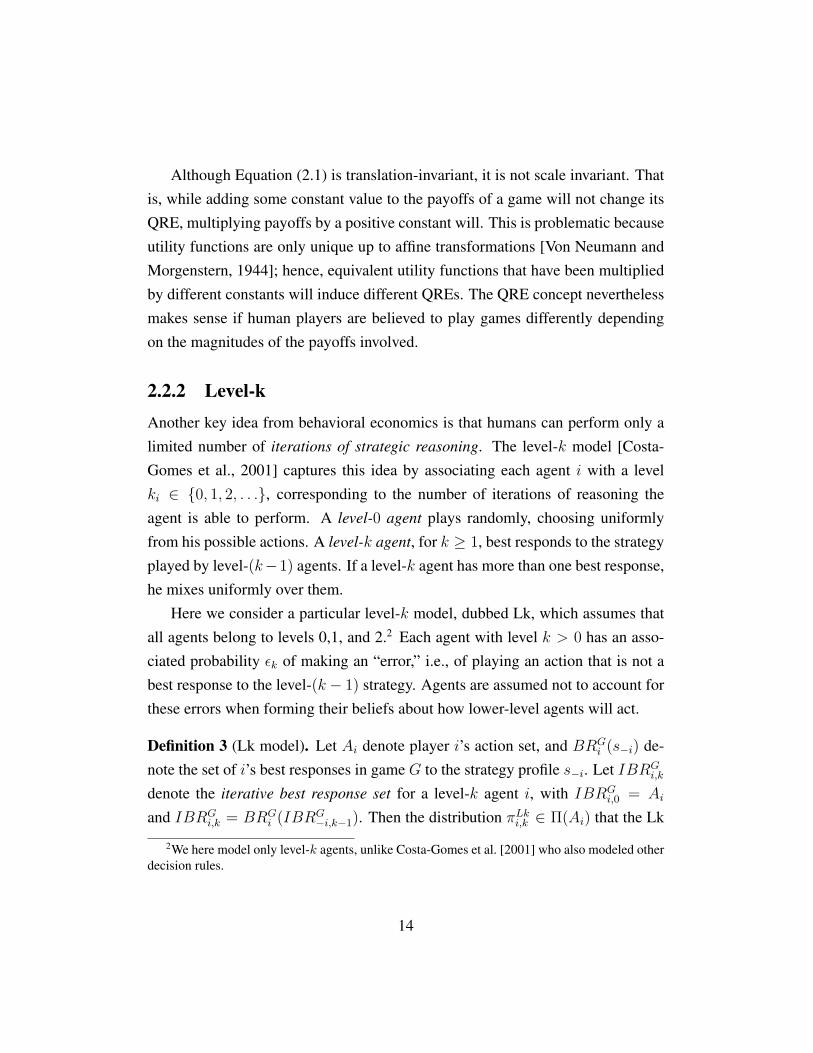
Although Equation (2.1) is translation-invariant, it is not scale invariant. Thatis, while adding some constant value to the payoffs of a game will not change itsQRE, multiplying payoffs by a positive constant will. This is problematic becauseutility functions are only unique up to affine transformations [Von Neumann andMorgenstern, 1944]; hence, equivalent utility functions that have been multipliedby different constants will induce different QREs. The QRE concept neverthelessmakes sense if human players are believed to play games differently dependingon the magnitudes of the payoffs involved.

2.2.2 Level-kAnother key idea from behavioral economics is that humans can perform only alimited number of iterations of strategic reasoning. The level-k model [Costa-Gomes et al., 2001] captures this idea by associating each agent i with a levelki ∈ {0, 1, 2, . . .}, corresponding to the number of iterations of reasoning theagent is able to perform. A level-0 agent plays randomly, choosing uniformlyfrom his possible actions. A level-k agent, for k ≥ 1, best responds to the strategyplayed by level-(k−1) agents. If a level-k agent has more than one best response,he mixes uniformly over them.

Here we consider a particular level-k model, dubbed Lk, which assumes thatall agents belong to levels 0,1, and 2.2 Each agent with level k > 0 has an asso-ciated probability εk of making an “error,” i.e., of playing an action that is not abest response to the level-(k − 1) strategy. Agents are assumed not to account forthese errors when forming their beliefs about how lower-level agents will act.

Definition 3 (Lk model). Let Ai denote player i’s action set, and BRGi (s−i) de-

note the set of i’s best responses in game G to the strategy profile s−i. Let IBRGi,k

denote the iterative best response set for a level-k agent i, with IBRGi,0 = Ai

and IBRGi,k = BRG

i (IBRG−i,k−1). Then the distribution πLki,k ∈ Π(Ai) that the Lk

2We here model only level-k agents, unlike Costa-Gomes et al. [2001] who also modeled otherdecision rules.

14

model predicts for a level-k agent i is defined as

πLki,0 (ai) = |Ai|−1,

πLki,k (ai) =

(1− εk)/|IBRGi,k| if ai ∈ IBRG

i,k,

εk/(|Ai| − |IBRGi,k|) otherwise.

The overall predicted distribution of actions is a weighted sum of the distributionsfor each level:

Pr(ai |G,α1, α2, ε1, ε2) =2∑`=0

α` · πLki,` (ai),

where α0 = 1 − α1 − α2. This model thus has 4 parameters: {α1, α2}, theproportions of level-1 and level-2 agents, and {ε1, ε2}, the error probabilities forlevel-1 and level-2 agents.

2.2.3 Cognitive HierarchyThe cognitive hierarchy model [Camerer et al., 2004], like level-k, models agentswith heterogeneous bounds on iterated reasoning. It differs from the level-k modelin two ways. First, according to this model agents do not make errors; each agentalways best responds to its beliefs. Second, agents of level-m best respond tothe full distribution of agents at the lower levels 0–(m − 1), rather than only tolevel-(m − 1) agents. More formally, every agent has an associated level m ∈{0, 1, 2, . . .}. Let f be a probability mass function describing the distribution ofthe levels in the population. Level-0 agents play uniformly at random. Level-magents (m ≥ 1) best respond to the strategies that would be played in a populationdescribed by the truncated probability mass function f(j | j < m).

Camerer et al. [2004] advocate a single-parameter restriction of the cognitivehierarchy model called Poisson-CH, in which f is a Poisson distribution.

Definition 4 (Poisson-CH model). Let πPCHi,m ∈ Π(Ai) be the distribution overactions predicted for an agent i with level m by the Poisson-CH model. Letf(m) = Poisson(m; τ). Let BRG

i (s−i) denote the set of i’s best responses in

15

game G to the strategy profile s−i. Let

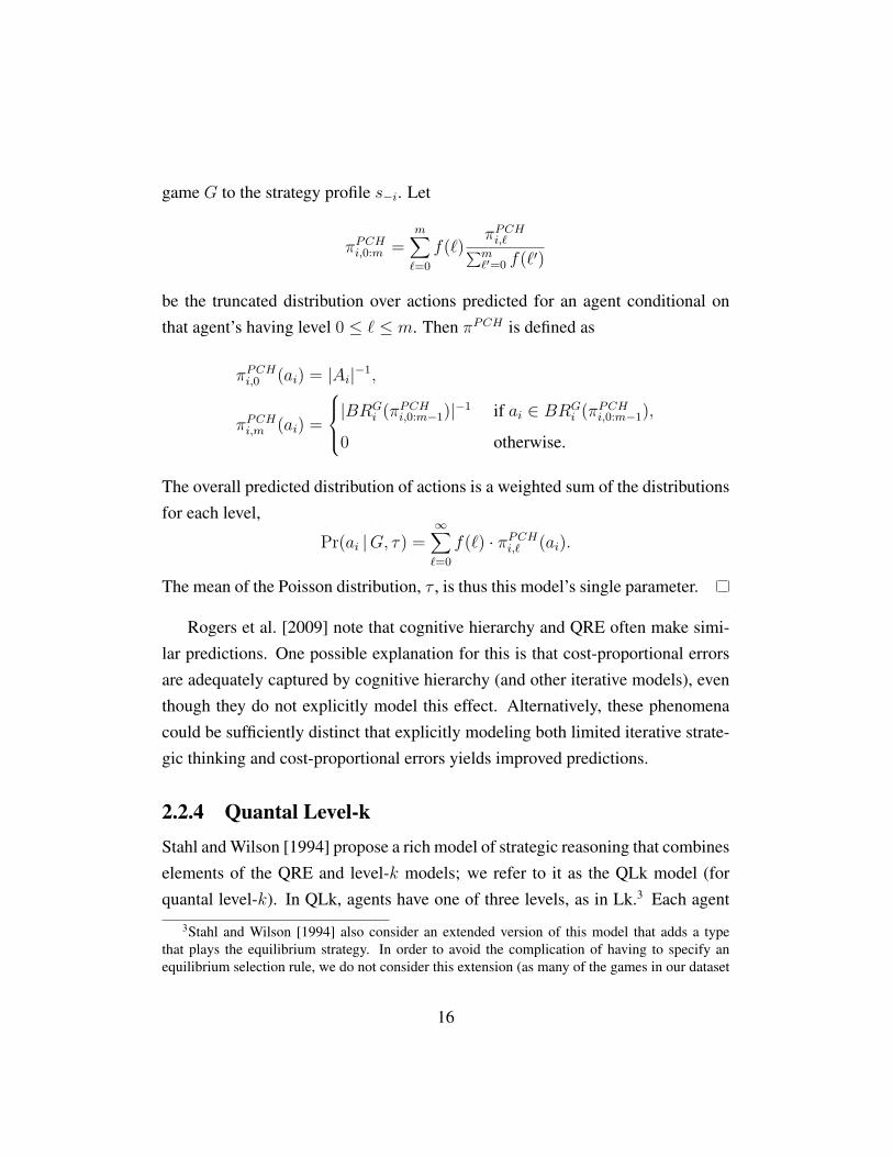
πPCHi,0:m =m∑`=0

f(`)πPCHi,`∑m`′=0 f(`′)

be the truncated distribution over actions predicted for an agent conditional onthat agent’s having level 0 ≤ ` ≤ m. Then πPCH is defined as

πPCHi,0 (ai) = |Ai|−1,

πPCHi,m (ai) =

|BRGi (πPCHi,0:m−1)|−1 if ai ∈ BRG

i (πPCHi,0:m−1),

0 otherwise.

The overall predicted distribution of actions is a weighted sum of the distributionsfor each level,

Pr(ai |G, τ) =∞∑`=0

f(`) · πPCHi,` (ai).

The mean of the Poisson distribution, τ , is thus this model’s single parameter.

Rogers et al. [2009] note that cognitive hierarchy and QRE often make simi-lar predictions. One possible explanation for this is that cost-proportional errorsare adequately captured by cognitive hierarchy (and other iterative models), eventhough they do not explicitly model this effect. Alternatively, these phenomenacould be sufficiently distinct that explicitly modeling both limited iterative strate-gic thinking and cost-proportional errors yields improved predictions.

2.2.4 Quantal Level-kStahl and Wilson [1994] propose a rich model of strategic reasoning that combineselements of the QRE and level-k models; we refer to it as the QLk model (forquantal level-k). In QLk, agents have one of three levels, as in Lk.3 Each agent

3Stahl and Wilson [1994] also consider an extended version of this model that adds a typethat plays the equilibrium strategy. In order to avoid the complication of having to specify anequilibrium selection rule, we do not consider this extension (as many of the games in our dataset

16

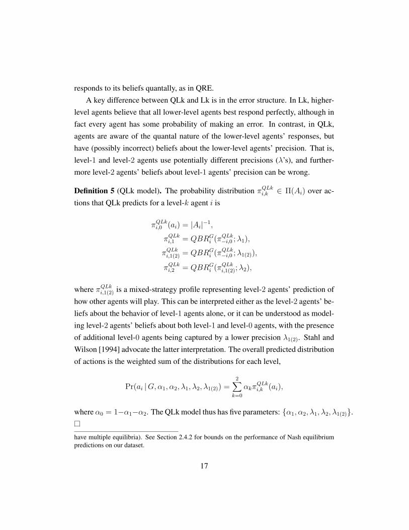
responds to its beliefs quantally, as in QRE.A key difference between QLk and Lk is in the error structure. In Lk, higher-

level agents believe that all lower-level agents best respond perfectly, although infact every agent has some probability of making an error. In contrast, in QLk,agents are aware of the quantal nature of the lower-level agents’ responses, buthave (possibly incorrect) beliefs about the lower-level agents’ precision. That is,level-1 and level-2 agents use potentially different precisions (λ’s), and further-more level-2 agents’ beliefs about level-1 agents’ precision can be wrong.

Definition 5 (QLk model). The probability distribution πQLki,k ∈ Π(Ai) over ac-tions that QLk predicts for a level-k agent i is

πQLki,0 (ai) = |Ai|−1,

πQLki,1 = QBRGi (πQLk−i,0 ;λ1),

πQLki,1(2) = QBRGi (πQLk−i,0 ;λ1(2)),

πQLki,2 = QBRGi (πQLki,1(2);λ2),

where πQLki,1(2) is a mixed-strategy profile representing level-2 agents’ prediction ofhow other agents will play. This can be interpreted either as the level-2 agents’ be-liefs about the behavior of level-1 agents alone, or it can be understood as model-ing level-2 agents’ beliefs about both level-1 and level-0 agents, with the presenceof additional level-0 agents being captured by a lower precision λ1(2). Stahl andWilson [1994] advocate the latter interpretation. The overall predicted distributionof actions is the weighted sum of the distributions for each level,

Pr(ai |G,α1, α2, λ1, λ2, λ1(2)) =2∑

k=0αkπ

QLki,k (ai),

where α0 = 1−α1−α2. The QLk model thus has five parameters: {α1, α2, λ1, λ2, λ1(2)}.

have multiple equilibria). See Section 2.4.2 for bounds on the performance of Nash equilibriumpredictions on our dataset.

17

2.2.5 Noisy IntrospectionGoeree and Holt [2004] propose a model called noisy introspection that combinescost-proportional errors and an iterative view of strategic cognition in a differentway. Rather than assuming a fixed limit on the number of iterations of strate-gic thinking, they instead model cognitive bounds by injecting noise into iteratedbeliefs about others’ beliefs and decisions, with the effect that deeper levels ofreasoning are assumed to be noisier. They then show that this process of noise in-jection converges to a unique prediction after a finite number of iterations, whichfor most games is relatively small.

Goeree and Holt also introduce a concrete version of this model, in whichdeeper levels of reasoning are exponentially noisier. We refer to this restrictedversion as the NI model.

Definition 6 (NI model). Define πNI,ni,k as

πNI,ni,k =

QBRGi (πNI,n−i,k+1;λ0/t

k) if k < n,

QBRGi (p0;λ0/t

n) otherwise,

where p0 is an arbitrary mixed profile, λ0 ≥ 0 is a precision, and t > 1 is a“telescoping” parameter that determines how quickly noise increases with depthof reasoning. Then the NI model predicts that each agent will play according to

πNIi = limn→∞

πNI,ni,0 .

For a fixed game G, precision λ0, and telescoping parameter t, this convergesto a unique strategy profile regardless of the choice of p0 (since in the limit theprecision becomes low enough to bring any profile arbitrarily close to the uniformdistribution.)

18

2.3 Comparing Models

2.3.1 Prediction FrameworkHow do we determine whether a behavioral model is well supported by exper-imental data? An experimental dataset D = {(Gi, {aij | j = 1, . . . , Ji}) | i =1, . . . , I} is a set containing I elements. Each element is a tuple containing agame Gi and a set of Ji pure actions aij , each played by a human subject in Gi.For symmetric games, we treat all actions as being played by the first player. Fornon-symmetric games, the player is implicit in the action being chosen (that is, Jicontains a separate entry for each of the first and second players’ actions). Thereis no reason to maintain the pairing of the play of a human player with that of hisopponent, as games are unrepeated. Recall that a behavioral model is a mappingfrom a game Gi and a vector of parameters θ to a predicted distribution over eachaction ai in Gi, which we denote Pr(ai |Gi, θ).

A behavioral model can only be used to make predictions when its parame-ters are instantiated. How should we set these parameters? Our goal is a modelthat produces accurate probability distributions over the actions of human agents,rather than simply determining the single action most likely to be played. Thismeans that we cannot score different models (or, equivalently, different parametersettings for the same model) using a criterion such as a 0–1 loss function (accu-racy), which asks how many actions were accurately predicted. (For example, the0–1 loss function evaluates models based purely upon which action is assignedthe highest probability, and does not take account of the probabilities assigned tothe other actions.) Instead, we evaluate a given model on a given dataset by like-

lihood. That is, we compute the probability of the observed actions according tothe distribution over actions predicted by the model. The higher the probabilityof the actual observations according to the prediction output by a model, the bet-ter the model predicted the observations. This takes account of the full predicteddistribution; in particular, for any given observed distribution, the prediction that

19

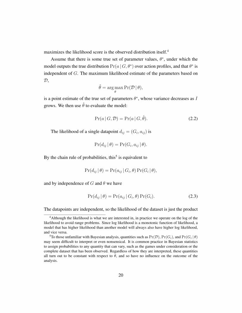
maximizes the likelihood score is the observed distribution itself.4

Assume that there is some true set of parameter values, θ∗, under which themodel outputs the true distribution Pr(a |G, θ∗) over action profiles, and that θ∗ isindependent of G. The maximum likelihood estimate of the parameters based onD,

θ = arg maxθ

Pr(D | θ),

is a point estimate of the true set of parameters θ∗, whose variance decreases as Igrows. We then use θ to evaluate the model:

Pr(a |G,D) = Pr(a |G, θ). (2.2)

The likelihood of a single datapoint dij = (Gi, aij) is

Pr(dij | θ) = Pr(Gi, aij | θ).

By the chain rule of probabilities, this5 is equivalent to

Pr(dij | θ) = Pr(aij |Gi, θ) Pr(Gi | θ),

and by independence of G and θ we have

Pr(dij | θ) = Pr(aij |Gi, θ) Pr(Gi). (2.3)

The datapoints are independent, so the likelihood of the dataset is just the product

4Although the likelihood is what we are interested in, in practice we operate on the log of thelikelihood to avoid range problems. Since log likelihood is a monotonic function of likelihood, amodel that has higher likelihood than another model will always also have higher log likelihood,and vice versa.

5To those unfamiliar with Bayesian analysis, quantities such as Pr(D), Pr(Gi), and Pr(Gi | θ)may seem difficult to interpret or even nonsensical. It is common practice in Bayesian statisticsto assign probabilities to any quantity that can vary, such as the games under consideration or thecomplete dataset that has been observed. Regardless of how they are interpreted, these quantitiesall turn out to be constant with respect to θ, and so have no influence on the outcome of theanalysis.

20

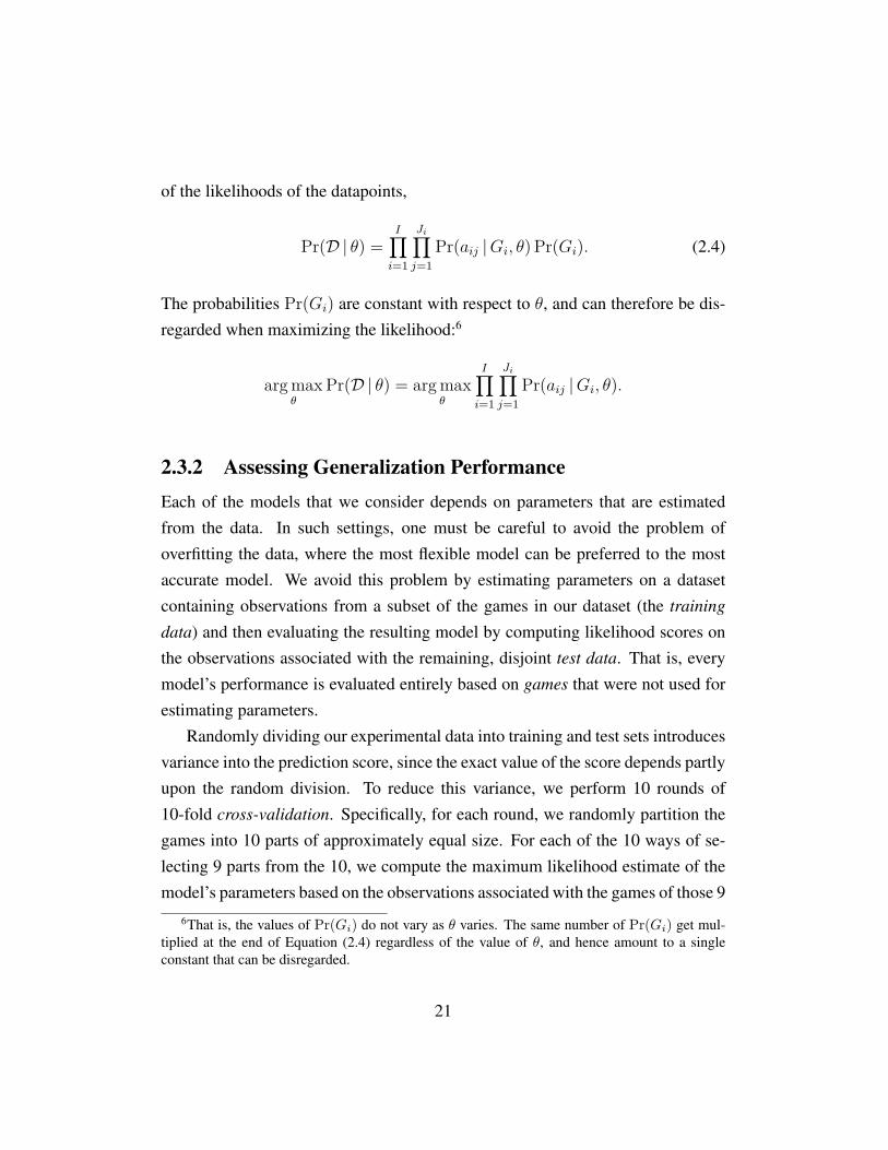
of the likelihoods of the datapoints,

Pr(D | θ) =I∏i=1

Ji∏j=1

Pr(aij |Gi, θ) Pr(Gi). (2.4)

The probabilities Pr(Gi) are constant with respect to θ, and can therefore be dis-regarded when maximizing the likelihood:6

arg maxθ

Pr(D | θ) = arg maxθ

I∏i=1

Ji∏j=1

Pr(aij |Gi, θ).

2.3.2 Assessing Generalization PerformanceEach of the models that we consider depends on parameters that are estimatedfrom the data. In such settings, one must be careful to avoid the problem ofoverfitting the data, where the most flexible model can be preferred to the mostaccurate model. We avoid this problem by estimating parameters on a datasetcontaining observations from a subset of the games in our dataset (the training

data) and then evaluating the resulting model by computing likelihood scores onthe observations associated with the remaining, disjoint test data. That is, everymodel’s performance is evaluated entirely based on games that were not used forestimating parameters.

Randomly dividing our experimental data into training and test sets introducesvariance into the prediction score, since the exact value of the score depends partlyupon the random division. To reduce this variance, we perform 10 rounds of10-fold cross-validation. Specifically, for each round, we randomly partition thegames into 10 parts of approximately equal size. For each of the 10 ways of se-lecting 9 parts from the 10, we compute the maximum likelihood estimate of themodel’s parameters based on the observations associated with the games of those 9

6That is, the values of Pr(Gi) do not vary as θ varies. The same number of Pr(Gi) get mul-tiplied at the end of Equation (2.4) regardless of the value of θ, and hence amount to a singleconstant that can be disregarded.

21

parts. We then determine the likelihood of the remaining part given the prediction.We call the average of this quantity across all 10 parts the cross-validated likeli-

hood. The average (across rounds) of the cross-validated likelihoods is distributedaccording to a Student’s-t distribution [see, e.g., Witten and Frank, 2000]. Wecompare the predictive power of different behavioral models on a given dataset bycomparing the average cross-validated likelihood of the dataset under each model.We say that one model predicts significantly better than another when the 95%confidence intervals for the average cross-validated likelihoods do not overlap.

2.4 Experimental SetupIn this section we describe the data and methods that we used in our model evalu-ations. We also describe a baseline model based on Nash equilibrium.

2.4.1 DataAs described in detail in Section 2.6, we conducted an exhaustive survey of papersthat make use of the five behavioral models we consider. We thereby identified tenlarge-scale, publicly available sets of human-subject experimental data [Stahl andWilson, 1994, 1995; Costa-Gomes et al., 1998; Goeree and Holt, 2001; Haruvyet al., 2001; Cooper and Van Huyck, 2003; Haruvy and Stahl, 2007; Costa-Gomesand Weizsacker, 2008; Stahl and Haruvy, 2008; Rogers et al., 2009]. We study allten7 of these datasets in this paper, and describe each briefly in what follows.

7 We identified an additional dataset [Costa-Gomes and Crawford, 2006] which we do not in-clude due to a computational issue. The games in this dataset had between 200 and 800 actions perplayer, which made it intractable to compute many solution concepts. As with Nash equilibrium,the main bottleneck in computing behavioral solution concepts is computing expected utilities.Each epoch of training for this dataset requires taking expected utility over up to 640, 000 out-comes per game, in contrast to between 9 and approximately 14, 000 outcomes per game in theALL10 dataset. We attempted to evaluate a coarse version of this data by binning similar actions;however, binning in this way results in games that are not strategically equivalent to the origi-nals (e.g., when multiple iterations of best response would result in the same binned action in thecoarsened games but different unbinned actions in the original games). The best way of addressingthis computational problem would be to represent the games compactly [e.g., Kearns et al., 2001;Koller and Milch, 2001; Jiang et al., 2011], such that expected utility can be computed efficiently

22

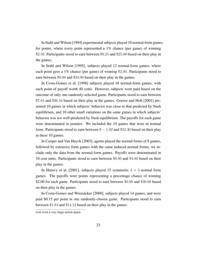
In Stahl and Wilson [1994] experimental subjects played 10 normal-form gamesfor points, where every point represented a 1% chance (per game) of winning$2.50. Participants stood to earn between $0.25 and $25.00 based on their play inthe games.

In Stahl and Wilson [1995], subjects played 12 normal-form games, whereeach point gave a 1% chance (per game) of winning $2.00. Participants stood toearn between $0.00 and $24.00 based on their play in the games.

In Costa-Gomes et al. [1998] subjects played 18 normal-form games, witheach point of payoff worth 40 cents. However, subjects were paid based on theoutcome of only one randomly-selected game. Participants stood to earn between$7.84 and $36.16 based on their play in the games. Goeree and Holt [2001] pre-sented 10 games in which subjects’ behavior was close to that predicted by Nashequilibrium, and 10 other small variations on the same games in which subjects’behavior was not well-predicted by Nash equilibrium. The payoffs for each gamewere denominated in pennies. We included the 10 games that were in normalform. Participants stood to earn between $− 1.02 and $23.30 based on their playin these 10 games.

In Cooper and Van Huyck [2003], agents played the normal forms of 8 games,followed by extensive form games with the same induced normal forms; we in-clude only the data from the normal-form games. Payoffs were denominated in10 cent units. Participants stood to earn between $0.80 and $4.80 based on theirplay in the games.

In Haruvy et al. [2001], subjects played 15 symmetric 3 × 3 normal formgames. The payoffs were points representing a percentage chance of winning$2.00 for each game. Participants stood to earn between $0.00 and $30.00 basedon their play in the games.

In Costa-Gomes and Weizsacker [2008], subjects played 14 games, and werepaid $0.15 per point in one randomly-chosen game. Participants stood to earnbetween $1.83 and $14.13 based on their play in the games.

over even a very large action space.

23

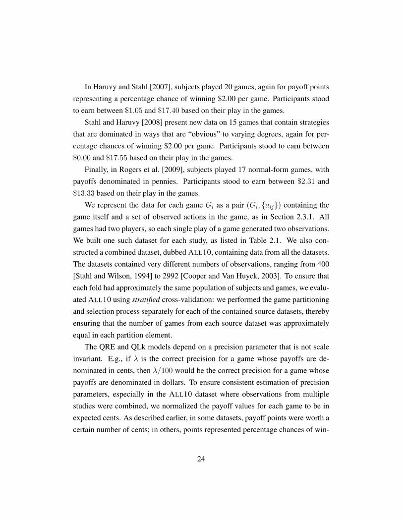
In Haruvy and Stahl [2007], subjects played 20 games, again for payoff pointsrepresenting a percentage chance of winning $2.00 per game. Participants stoodto earn between $1.05 and $17.40 based on their play in the games.

Stahl and Haruvy [2008] present new data on 15 games that contain strategiesthat are dominated in ways that are “obvious” to varying degrees, again for per-centage chances of winning $2.00 per game. Participants stood to earn between$0.00 and $17.55 based on their play in the games.

Finally, in Rogers et al. [2009], subjects played 17 normal-form games, withpayoffs denominated in pennies. Participants stood to earn between $2.31 and$13.33 based on their play in the games.

We represent the data for each game Gi as a pair (Gi, {aij}) containing thegame itself and a set of observed actions in the game, as in Section 2.3.1. Allgames had two players, so each single play of a game generated two observations.We built one such dataset for each study, as listed in Table 2.1. We also con-structed a combined dataset, dubbed ALL10, containing data from all the datasets.The datasets contained very different numbers of observations, ranging from 400[Stahl and Wilson, 1994] to 2992 [Cooper and Van Huyck, 2003]. To ensure thateach fold had approximately the same population of subjects and games, we evalu-ated ALL10 using stratified cross-validation: we performed the game partitioningand selection process separately for each of the contained source datasets, therebyensuring that the number of games from each source dataset was approximatelyequal in each partition element.

The QRE and QLk models depend on a precision parameter that is not scaleinvariant. E.g., if λ is the correct precision for a game whose payoffs are de-nominated in cents, then λ/100 would be the correct precision for a game whosepayoffs are denominated in dollars. To ensure consistent estimation of precisionparameters, especially in the ALL10 dataset where observations from multiplestudies were combined, we normalized the payoff values for each game to be inexpected cents. As described earlier, in some datasets, payoff points were worth acertain number of cents; in others, points represented percentage chances of win-

24

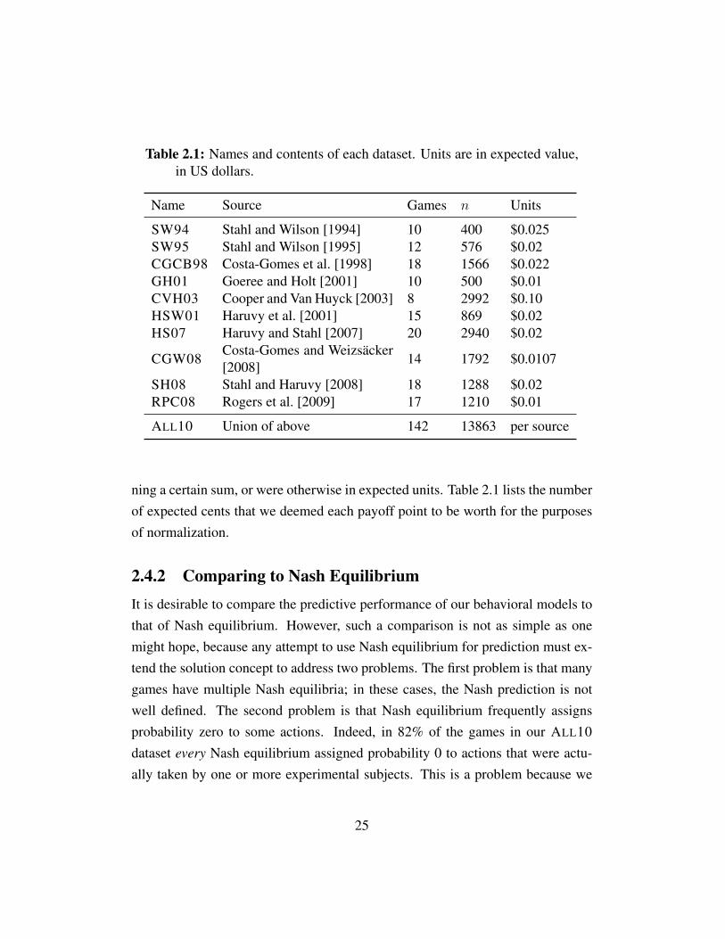
Table 2.1: Names and contents of each dataset. Units are in expected value,in US dollars.

Name Source Games n Units

SW94 Stahl and Wilson [1994] 10 400 $0.025SW95 Stahl and Wilson [1995] 12 576 $0.02CGCB98 Costa-Gomes et al. [1998] 18 1566 $0.022GH01 Goeree and Holt [2001] 10 500 $0.01CVH03 Cooper and Van Huyck [2003] 8 2992 $0.10HSW01 Haruvy et al. [2001] 15 869 $0.02HS07 Haruvy and Stahl [2007] 20 2940 $0.02

CGW08Costa-Gomes and Weizsacker[2008] 14 1792 $0.0107

SH08 Stahl and Haruvy [2008] 18 1288 $0.02RPC08 Rogers et al. [2009] 17 1210 $0.01

ALL10 Union of above 142 13863 per source

ning a certain sum, or were otherwise in expected units. Table 2.1 lists the numberof expected cents that we deemed each payoff point to be worth for the purposesof normalization.

2.4.2 Comparing to Nash EquilibriumIt is desirable to compare the predictive performance of our behavioral models tothat of Nash equilibrium. However, such a comparison is not as simple as onemight hope, because any attempt to use Nash equilibrium for prediction must ex-tend the solution concept to address two problems. The first problem is that manygames have multiple Nash equilibria; in these cases, the Nash prediction is notwell defined. The second problem is that Nash equilibrium frequently assignsprobability zero to some actions. Indeed, in 82% of the games in our ALL10dataset every Nash equilibrium assigned probability 0 to actions that were actu-ally taken by one or more experimental subjects. This is a problem because we

25

assess the quality of a model by how well it explains the data; unmodified, Nashequilibrium model considers our experimental data to be impossible, and hencereceives a likelihood of zero.

We addressed the second problem by augmenting the Nash equilibrium so-lution concept to say that with some probability, each player chooses an actionuniformly at random; this prevents the solution concept from assessing any exper-imental data as impossible. This probability is a free parameter of the model; aswe did with behavioral models, we fit this parameter using maximum likelihoodestimation on a training set. We thus call the model Nash Equilibrium with Error(NEE). We sidestepped the first problem by assuming that agents always coordi-nate to play an equilibrium and by reporting statistics across different equilibria.Specifically, we report the performance achieved by choosing the equilibrium thatrespectively best and worst fit the test data, thereby giving upper and lower boundson the test-set performance achievable by any Nash-based prediction. (Note thatbecause we “cheat” by choosing equilibria based on test-set performance, thesemodels are not able to generalize to new data, and hence cannot be used in prac-tice.) Finally, we also reported the prediction performance on the test data, aver-aged over all of the Nash equilibria of the game.8

2.4.3 Computational EnvironmentWe performed computation using WestGrid (www.westgrid.ca), primarily on theorcinus cluster, which has 9600 64-bit Intel Xeon CPU cores. We used GAMBIT

[McKelvey et al., 2007] to compute QRE and to enumerate the Nash equilibria ofgames, and computed maximum likelihood estimates using the Covariance Ma-trix Adaptation Evolution Strategy (CMA-ES) algorithm [Hansen and Ostermeier,

8One might wonder whether the ε-equilibrium solution concept [e.g., Shoham and Leyton-Brown, 2008, Section 3.4.7] solves either of these problems. It does not. First, ε-equilibriumcan still assign probability 0 to some actions, unlike NEE which will always assign at least ε.Second, relaxing the equilibrium concept only increases the number of equilibria; indeed, everygame has infinitely many ε-equilibria for any ε > 0. Furthermore, to our knowledge, no algorithmfor characterizing this set exists, making equilibrium selection impractical.

26

2001].

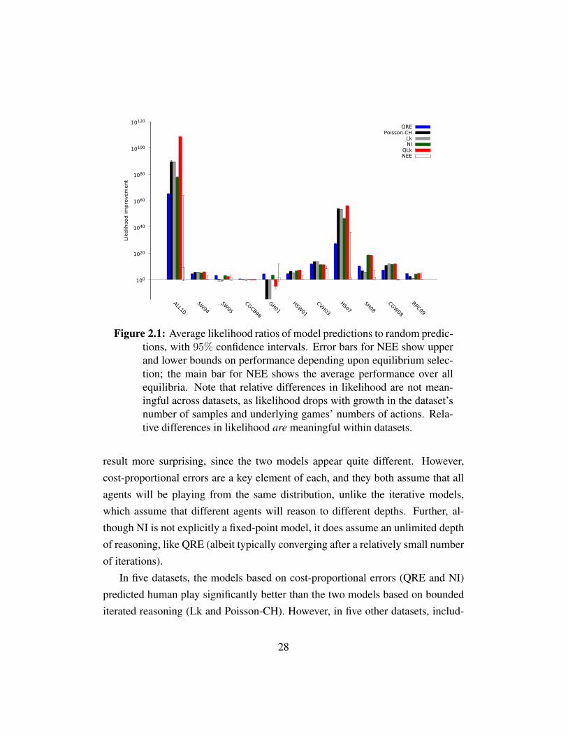
2.5 Model ComparisonsIn this section we describe the results of our experiments comparing the predictiveperformance of the five behavioral models from Section 2.2 and of the Nash-basedmodels of Section 2.4.2. Figure 2.1 compares our behavioral and Nash-basedmodels. For each model and each dataset, we give the factor by which the datasetwas judged more likely according to the model’s prediction than it was accord-ing to a uniform random prediction. Thus, for example, the ALL10 dataset wasfound to be approximately 1090 times more likely according to Poisson-CH’s pre-diction than according to a uniform random prediction. For the Nash Equilibriumwith Error model, the error bars show the upper and lower bounds on predictiveperformance obtained by selecting an equilibrium to maximize or minimize test-set performance, and the main bar shows the expected predictive performance ofselecting an equilibrium uniformly at random. For other models, the error bars in-dicate 95% confidence intervals across cross-validation partitions; in most cases,these intervals are imperceptibly narrow.

2.5.1 Comparing Behavioral ModelsPoisson-CH and Lk had very similar performance in most datasets. In one waythis is an intuitive result, since the models are very similar to each other. Poisson-CH and Lk had very similar performance in most datasets. In one way this is anintuitive result, since the models are very similar to each other. On the other hand,it suggests that the distinction between reasoning about just one lower level versusreasoning about the distribution of all lower levels, and the distinct error models,does not make much difference, which is perhaps less obvious.

QRE and NI tended to perform well on the same datasets. On all but twodatasets (HSW01 and CGW08), the ordering between QRE and the iterativemodels was the same as between NI and the iterative models. We found this

27

100

1020

1040

1060

1080

10100

10120

ALL10

SW94

SW95

CGCB98

GH01

HSW01

CVH03

HS07SH08

CGW08

RPC09

Like

lihood

im

pro

vem

ent

QREPoisson-CH

LkNI

QLkNEE

Figure 2.1: Average likelihood ratios of model predictions to random predic-tions, with 95% confidence intervals. Error bars for NEE show upperand lower bounds on performance depending upon equilibrium selec-tion; the main bar for NEE shows the average performance over allequilibria. Note that relative differences in likelihood are not mean-ingful across datasets, as likelihood drops with growth in the dataset’snumber of samples and underlying games’ numbers of actions. Rela-tive differences in likelihood are meaningful within datasets.

result more surprising, since the two models appear quite different. However,cost-proportional errors are a key element of each, and they both assume that allagents will be playing from the same distribution, unlike the iterative models,which assume that different agents will reason to different depths. Further, al-though NI is not explicitly a fixed-point model, it does assume an unlimited depthof reasoning, like QRE (albeit typically converging after a relatively small numberof iterations).

In five datasets, the models based on cost-proportional errors (QRE and NI)predicted human play significantly better than the two models based on boundediterated reasoning (Lk and Poisson-CH). However, in five other datasets, includ-

28

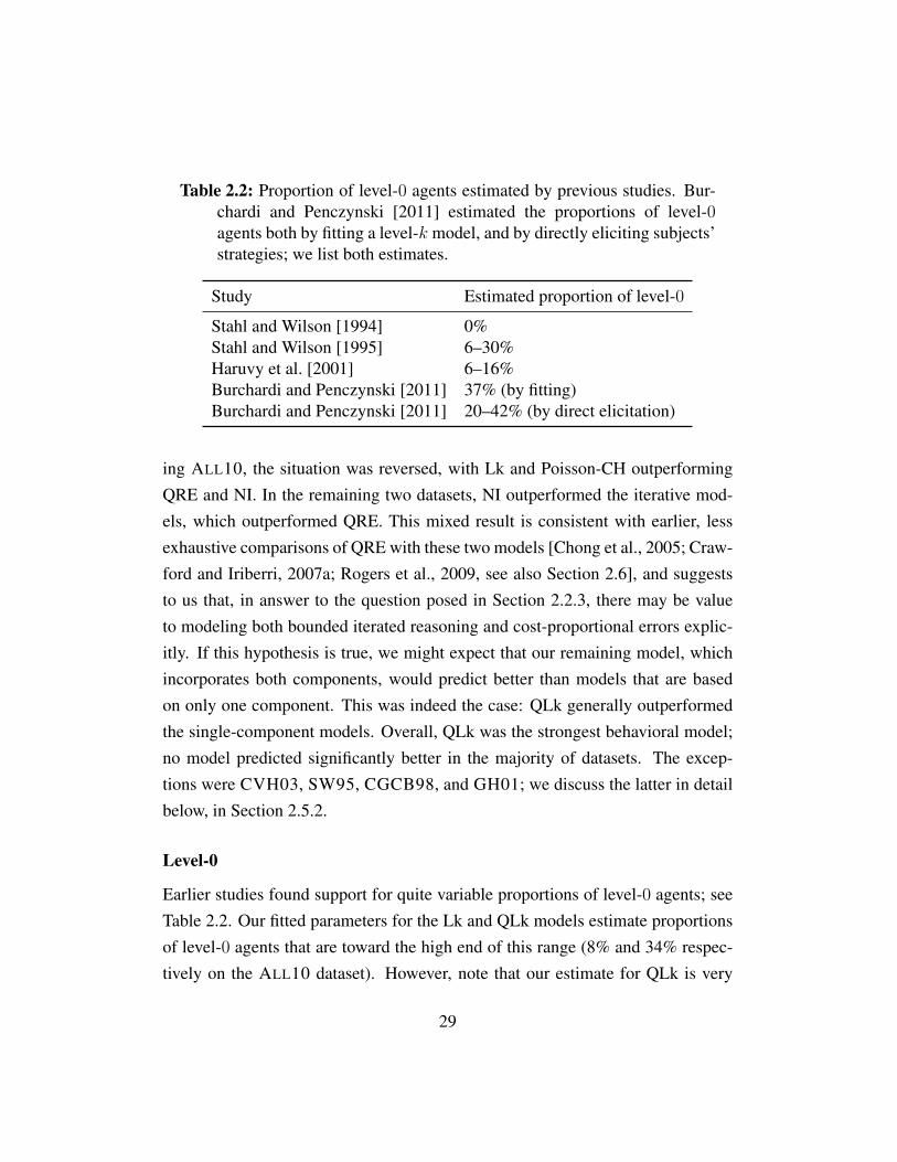
Table 2.2: Proportion of level-0 agents estimated by previous studies. Bur-chardi and Penczynski [2011] estimated the proportions of level-0agents both by fitting a level-k model, and by directly eliciting subjects’strategies; we list both estimates.

Study Estimated proportion of level-0Stahl and Wilson [1994] 0%Stahl and Wilson [1995] 6–30%Haruvy et al. [2001] 6–16%Burchardi and Penczynski [2011] 37% (by fitting)Burchardi and Penczynski [2011] 20–42% (by direct elicitation)

ing ALL10, the situation was reversed, with Lk and Poisson-CH outperformingQRE and NI. In the remaining two datasets, NI outperformed the iterative mod-els, which outperformed QRE. This mixed result is consistent with earlier, lessexhaustive comparisons of QRE with these two models [Chong et al., 2005; Craw-ford and Iriberri, 2007a; Rogers et al., 2009, see also Section 2.6], and suggeststo us that, in answer to the question posed in Section 2.2.3, there may be valueto modeling both bounded iterated reasoning and cost-proportional errors explic-itly. If this hypothesis is true, we might expect that our remaining model, whichincorporates both components, would predict better than models that are basedon only one component. This was indeed the case: QLk generally outperformedthe single-component models. Overall, QLk was the strongest behavioral model;no model predicted significantly better in the majority of datasets. The excep-tions were CVH03, SW95, CGCB98, and GH01; we discuss the latter in detailbelow, in Section 2.5.2.

Level-0

Earlier studies found support for quite variable proportions of level-0 agents; seeTable 2.2. Our fitted parameters for the Lk and QLk models estimate proportionsof level-0 agents that are toward the high end of this range (8% and 34% respec-tively on the ALL10 dataset). However, note that our estimate for QLk is very

29

similar to the fitted estimate of Burchardi and Penczynski [2011], and comfort-ably within the range that they estimated by directly evaluating subjects’ elicitedstrategies in a single game. We analyze the full distributions of parameter valuesin Chapter 3. In contrast to our estimates, the number of level-0 agents in the pop-ulation is typically assumed to be negligible in studies that use an iterative modelof behavior. Indeed, some studies [e.g., Crawford and Iriberri, 2007b] fix thenumber of level-0 agents to be 0. Thus, one possible interpretation of our higherestimates of level-0 agents is as evidence of a misspecified model. For example,Poisson-CH uses level-0 agents as the only source of noisy responses. However,we estimated substantial proportions of level-0 agents even for models (Lk andQLk) that include explicit error structures. We thus believe that the alternative—the possibility that these results point to a substantial frequency of nonstrategicbehavior9—must be taken seriously.

2.5.2 Comparing to Nash EquilibriumIt is already widely believed that Nash equilibrium—especially without refinements—is a poor description of humans’ initial play in normal-form games [e.g., Goereeand Holt, 2001]. Nevertheless, for the sake of completeness, we also evaluatedthe predictive power of Nash equilibrium with error on our datasets. Referringagain to Figure 2.1, we see that NEE’s predictions were worse than those of ev-ery behavioral model on every dataset except SW95 and CGCB98. NEE’s upperbound—using the post-hoc best equilibrium—was significantly worse than QLk’sperformance on every dataset except SW95, CGCB98, RPC09, and GH01.

NEE’s strong performance on SW95 was surprising; it may have been a resultof the unusual subject pool, which consisted of fourth and fifth year undergraduatefinance and accounting majors. In contrast, it is unsurprising that NEE performedwell on GH01, since this distribution was deliberately constructed so that human

9Although the models we present here typically specify level-0 behavior as uniform randomchoice, applications sometimes specify other nonstrategic level-0 behavior [e.g., Crawford andIriberri, 2007a; Arad and Rubinstein, 2012].

30

10-25

10-20

10-15

10-10

10-5

100

105

1010

1015

GH01 Treasure Contradiction

Like

lihood

im

pro

vem

ent

QREPoisson-CH

LkNI

QLkNEE

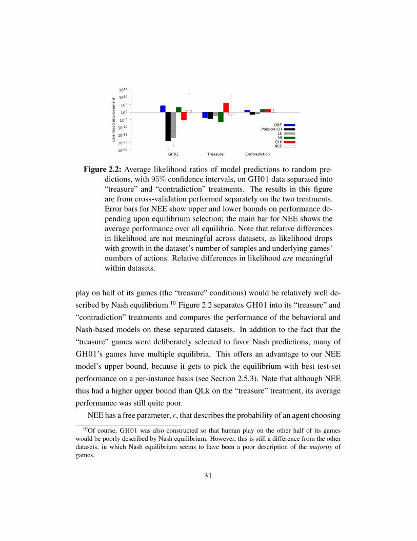
Figure 2.2: Average likelihood ratios of model predictions to random pre-dictions, with 95% confidence intervals, on GH01 data separated into“treasure” and “contradiction” treatments. The results in this figureare from cross-validation performed separately on the two treatments.Error bars for NEE show upper and lower bounds on performance de-pending upon equilibrium selection; the main bar for NEE shows theaverage performance over all equilibria. Note that relative differencesin likelihood are not meaningful across datasets, as likelihood dropswith growth in the dataset’s number of samples and underlying games’numbers of actions. Relative differences in likelihood are meaningfulwithin datasets.

play on half of its games (the “treasure” conditions) would be relatively well de-scribed by Nash equilibrium.10 Figure 2.2 separates GH01 into its “treasure” and“contradiction” treatments and compares the performance of the behavioral andNash-based models on these separated datasets. In addition to the fact that the“treasure” games were deliberately selected to favor Nash predictions, many ofGH01’s games have multiple equilibria. This offers an advantage to our NEEmodel’s upper bound, because it gets to pick the equilibrium with best test-setperformance on a per-instance basis (see Section 2.5.3). Note that although NEEthus had a higher upper bound than QLk on the “treasure” treatment, its averageperformance was still quite poor.

NEE has a free parameter, ε, that describes the probability of an agent choosing

10Of course, GH01 was also constructed so that human play on the other half of its gameswould be poorly described by Nash equilibrium. However, this is still a difference from the otherdatasets, in which Nash equilibrium seems to have been a poor description of the majority ofgames.

31

an action uniformly at random. If Nash equilibrium were a good tool for predict-ing human behavior, we would expect to find this parameter set to a low value; incontrast, the values of ε that maximize NEE’s performance were extremely high.On the ALL10 dataset, a value of ε = 0.87 maximized NEE’s average-case perfor-mance. Even best-case performance, which is computed by choosing the post-hocperformance-maximizing equilibrium for each game, was optimized by ε = 0.64.Thus, the fact that well over half of NEE’s prediction consists of the uniform noiseterm provides a strong argument against using Nash equilibrium to predict initialplay. This is especially true as the agents within a Nash equilibrium do not takeothers’ noisiness into account, which makes it difficult to interpret ε as a measureof level-0 play rather than of model misspecification.

2.5.3 Dataset CompositionAs we have already seen in the case of GH01, model performance was sensitive tochoices made by the authors of our various datasets about which games to study.One way to control for such choices is to partition our set of games according toimportant game properties, and to evaluate model performance in each partition.In this section we describe such an analysis.

Overall, our datasets spanned 142 games. The vast majority of these gamesare matrix games, deliberately lacking inherent meaning in order to avoid framingeffects. (Indeed, some studies [e.g., Rogers et al., 2009] even avoid focal payoffslike 0 and 100.) For the most part, these games were chosen to vary accordingto dominance solvability and equilibrium structure. In particular, most datasetauthors were concerned with (1) whether a game could be solved by iterated re-moval of dominated strategies (either strict or weak) and with how many steps ofiteration were required; and (2) the number and type of Nash equilibria that eachgame possesses.11

11There were two exceptions. The first was Goeree and Holt [2001], who chose games that hadboth equilibria that human subjects find intuitive and strategically equivalent variations of thesegames whose equilibria human subjects find counterintuitive. The second exception was Cooperand Van Huyck [2003], whose normal form games were based on an exhaustive enumeration of

32

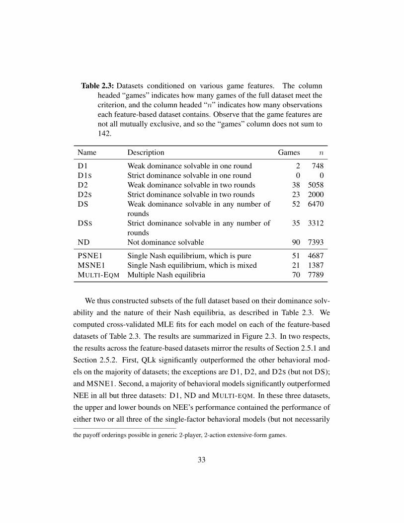
Table 2.3: Datasets conditioned on various game features. The columnheaded “games” indicates how many games of the full dataset meet thecriterion, and the column headed “n” indicates how many observationseach feature-based dataset contains. Observe that the game features arenot all mutually exclusive, and so the “games” column does not sum to142.

Name Description Games n

D1 Weak dominance solvable in one round 2 748D1S Strict dominance solvable in one round 0 0D2 Weak dominance solvable in two rounds 38 5058D2S Strict dominance solvable in two rounds 23 2000DS Weak dominance solvable in any number of

rounds52 6470

DSS Strict dominance solvable in any number ofrounds

35 3312

ND Not dominance solvable 90 7393

PSNE1 Single Nash equilibrium, which is pure 51 4687MSNE1 Single Nash equilibrium, which is mixed 21 1387MULTI-EQM Multiple Nash equilibria 70 7789

We thus constructed subsets of the full dataset based on their dominance solv-ability and the nature of their Nash equilibria, as described in Table 2.3. Wecomputed cross-validated MLE fits for each model on each of the feature-baseddatasets of Table 2.3. The results are summarized in Figure 2.3. In two respects,the results across the feature-based datasets mirror the results of Section 2.5.1 andSection 2.5.2. First, QLk significantly outperformed the other behavioral mod-els on the majority of datasets; the exceptions are D1, D2, and D2S (but not DS);and MSNE1. Second, a majority of behavioral models significantly outperformedNEE in all but three datasets: D1, ND and MULTI-EQM. In these three datasets,the upper and lower bounds on NEE’s performance contained the performance ofeither two or all three of the single-factor behavioral models (but not necessarily

the payoff orderings possible in generic 2-player, 2-action extensive-form games.

33

QLk). It is unsurprising that NEE’s upper and lower bounds were widely sepa-rated on the MULTI-EQM dataset, since the more equilibria a game has, the morevariation there can be in these equilibria’s post-hoc performance; NEE’s strongbest-case performance on this dataset should similarly reflect this variation. Itturns out that 55 of the 90 games (and 4731 of the 7393 observations) in the NDdataset are from the MULTI-EQM dataset, which likely explains NEE’s high upperbound in that dataset as well. Indeed, this analysis helps to explain some of ourprevious observations about the GH01 dataset. NEE contains all other modelsin its performance bounds in this dataset, and in addition to the fact that half thedataset’s games (the “treasure” treatments) that were chosen for consistency withNash equilibrium, some of the other games (the “contradiction” treatments) turnout to have multiple equilibria. Overall, the overlap between GH01 and MULTI-EQM is 5 games out of 10, and 250 observations out of 500.

Unlike in the per-dataset comparisons of Section 2.5.1, both of our iterativesingle-factor models (Poisson-CH and Lk) significantly outperformed QRE in al-most every feature-based dataset, with D2S and DSS as the only exceptions; inD2S, QRE outperformed all other models, and in DSS QRE was significantlyoutperformed by Lk but not Poisson-CH. One possible explanation is that the fil-tering features are all biased toward iterative models. However, it seems unlikelythat, e.g., both dominance-solvability and dominance-nonsolvability are biasedtoward iterative models. Another possibility is that iterative models are a bet-ter model of human behavior, but the cost-proportional error model of QRE issufficiently superior to the respectively simple and non-existent error models ofLk and Poisson-CH that it outperforms on many datasets that mix game types.Or, similarly, iterative models may fit very differently on dominance solvable andnon-dominance solvable games; in this case, they would perform very poorly onmixed data. We explore this last possibility in more detail in Section 3.3.1.

34

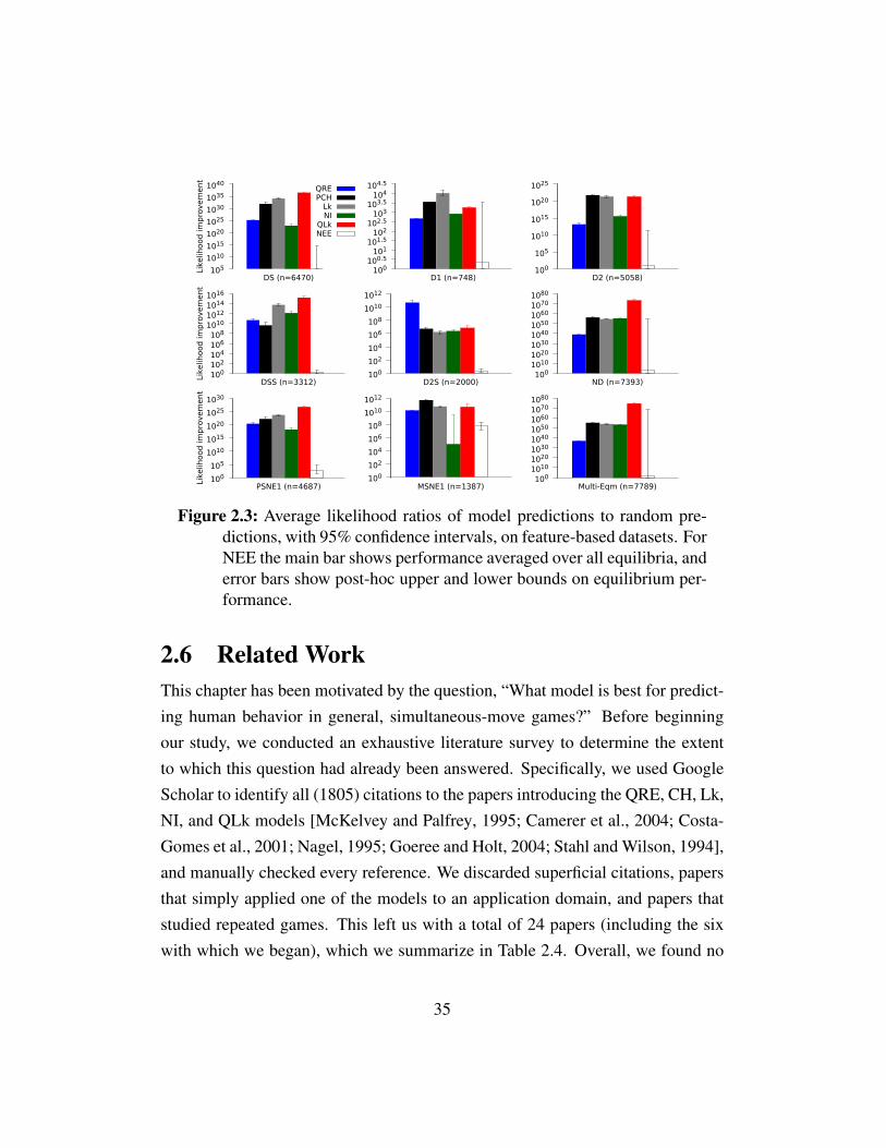
105

1010

1015

1020

1025

1030

1035

1040

Like

lihood

im

pro

vem

ent

DS (n=6470)

QREPCH

LkNI

QLkNEE

100100.5

101101.5

102102.5

103103.5

104104.5

D1 (n=748)100

105

1010

1015

1020

1025

D2 (n=5058)

100102104106108

1010101210141016

Like

lihood

im

pro

vem

ent

DSS (n=3312)100

102

104

106

108

1010

1012

D2S (n=2000)100

10101020103010401050106010701080

ND (n=7393)

100

105

1010

1015

1020

1025

1030

Like

lihood

im

pro

vem

ent

PSNE1 (n=4687)100

102

104

106

108

1010

1012

MSNE1 (n=1387)100

10101020103010401050106010701080

Multi-Eqm (n=7789)

Figure 2.3: Average likelihood ratios of model predictions to random pre-dictions, with 95% confidence intervals, on feature-based datasets. ForNEE the main bar shows performance averaged over all equilibria, anderror bars show post-hoc upper and lower bounds on equilibrium per-formance.

2.6 Related WorkThis chapter has been motivated by the question, “What model is best for predict-ing human behavior in general, simultaneous-move games?” Before beginningour study, we conducted an exhaustive literature survey to determine the extentto which this question had already been answered. Specifically, we used GoogleScholar to identify all (1805) citations to the papers introducing the QRE, CH, Lk,NI, and QLk models [McKelvey and Palfrey, 1995; Camerer et al., 2004; Costa-Gomes et al., 2001; Nagel, 1995; Goeree and Holt, 2004; Stahl and Wilson, 1994],and manually checked every reference. We discarded superficial citations, papersthat simply applied one of the models to an application domain, and papers thatstudied repeated games. This left us with a total of 24 papers (including the sixwith which we began), which we summarize in Table 2.4. Overall, we found no

35

paper that compared the predictive performance of all six models. Indeed, thereare two senses in which the literature focuses on different issues. First, it appearsto be more concerned with explaining behavior than with predicting it. Thus, com-parisons of out-of-sample prediction performance were rare. Here we describe theonly exceptions that we found:

• Stahl and Wilson [1995] evaluated prediction performance on 3 games usingparameters fit from the other games;

• Morgan and Sefton [2002] and Hahn et al. [2010] evaluated prediction per-formance using held-out test data;

• Camerer et al. [2004] and Chong et al. [2005] computed likelihoods on eachindividual game in their datasets after using models fit to the n−1 remaininggames;

• Crawford and Iriberri [2007a] compared the performance of two models bytraining each model on each game in their dataset individually, and thenevaluating the performance of each of these n trained models on each of then− 1 other individual games; and

• Camerer et al. [2011] evaluated the performance of QRE and cognitive hi-erarchy variants on one experimental treatment using parameters estimatedon two separate experimental treatments.

Second, most of the papers compared a single one of the five models (often withvariations) to Nash equilibrium. Indeed, only nine of the 25 studies (see the bot-tom portion of Table 2.4) compared more than one of the six key models, andnone of these considered QLk. Only three of these studies explicitly comparedthe prediction performance of more than one of the six models [Chong et al.,2005; Crawford and Iriberri, 2007a; Camerer et al., 2011]; the remaining six per-formed comparisons in terms of training set fit [Camerer et al., 2001; Goereeand Holt, 2004; Costa-Gomes and Weizsacker, 2008; Costa-Gomes et al., 2009;Rogers et al., 2009; Breitmoser, 2012].

36

Rogers et al. [2009] proposed a unifying framework that generalizes bothPoisson-CH and QRE, and compared the fit of several variations within this frame-work. Notably, their framework allows for quantal response within a cognitive hi-erarchy model. Their work is thus similar to our own search over a system of QLkvariants in Chapter 4, but there are several differences. First, we compared out-of-sample prediction performance, not in-sample fit. Second, Rogers et al. restrictedthe distributions of types to be grid, uniform, or Poisson distributions, whereas weconsidered unconstrained discrete distributions over levels. Third, they requireddifferent agent types to have different precisions, while we did not. Finally, weconsidered level-k beliefs as well as cognitive hierarchy beliefs, whereas theyconsidered only cognitive hierarchy belief models (although their framework inprinciple allows for both).

One line of work from the computer science literature also meets our criteriaof predicting action choices and modeling human behavior [Altman et al., 2006].This approach learns association rules between agents’ actions in different gamesto predict how an agent will play based on its actions in earlier games. We did notconsider this approach in our study, as it requires data that identifies agents acrossgames, and cannot make predictions for games that are not in the training dataset.Nevertheless, other machine-learning-based methods can clearly be extended toapply to our setting; we explore such an extension in Chapter 6.

2.7 ConclusionsTo our knowledge, ours is the first study to address the question of which of theQRE, level-k, cognitive hierarchy, noisy introspection, and quantal level-k behav-ioral models is best suited to predicting unseen human play of normal-form games.We explored the prediction performance of these models, along with several mod-ifications. We found that bounded iterated reasoning and cost-proportional errorsare both valuable ingredients in a predictive model of human game theoretic be-havior: the best-performing model that we studied (QLk) combines both of theseelements.

37

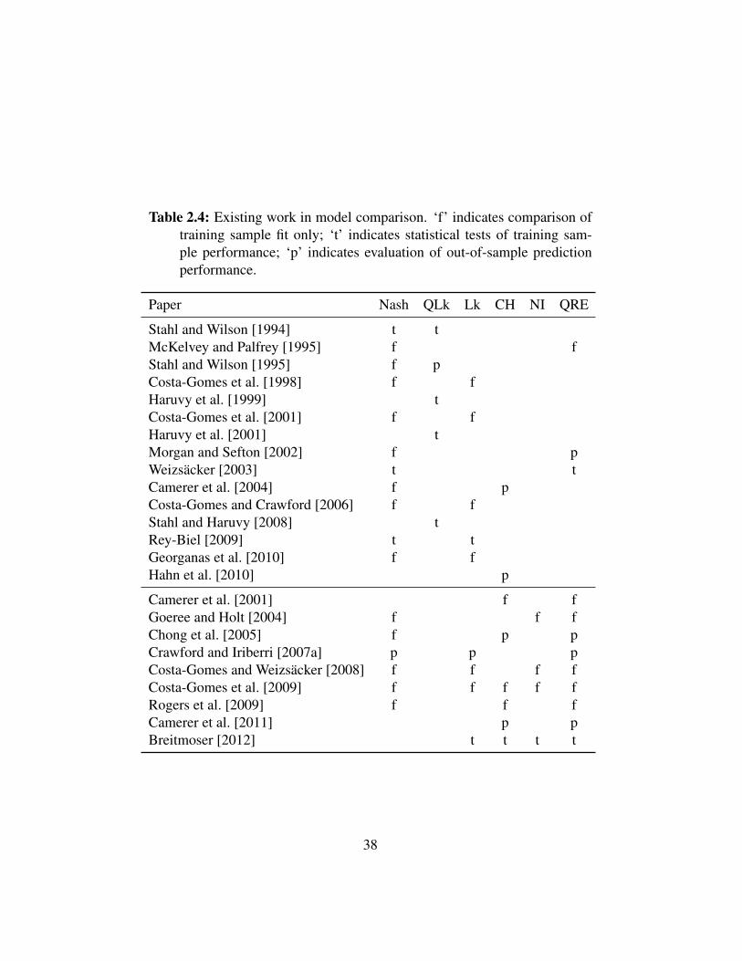
Table 2.4: Existing work in model comparison. ‘f’ indicates comparison oftraining sample fit only; ‘t’ indicates statistical tests of training sam-ple performance; ‘p’ indicates evaluation of out-of-sample predictionperformance.

Paper Nash QLk Lk CH NI QRE

Stahl and Wilson [1994] t tMcKelvey and Palfrey [1995] f fStahl and Wilson [1995] f pCosta-Gomes et al. [1998] f fHaruvy et al. [1999] tCosta-Gomes et al. [2001] f fHaruvy et al. [2001] tMorgan and Sefton [2002] f pWeizsacker [2003] t tCamerer et al. [2004] f pCosta-Gomes and Crawford [2006] f fStahl and Haruvy [2008] tRey-Biel [2009] t tGeorganas et al. [2010] f fHahn et al. [2010] p

Camerer et al. [2001] f fGoeree and Holt [2004] f f fChong et al. [2005] f p pCrawford and Iriberri [2007a] p p pCosta-Gomes and Weizsacker [2008] f f f fCosta-Gomes et al. [2009] f f f f fRogers et al. [2009] f f fCamerer et al. [2011] p pBreitmoser [2012] t t t t

38

Chapter 3

Parameter Analysis of BehavioralGame Theoretic Models

3.1 IntroductionMaking good predictions from behavioral models depends upon obtaining goodestimates of model parameters. These estimates can also be useful in themselves,helping researchers to understand both how people behave in strategic situationsand whether a model’s behavior aligns or clashes with its intended economic inter-pretation. Unfortunately, the method we have used so far—maximum likelihoodestimation, i.e., finding a single set of parameters that best explains the trainingset—is not a good way of gaining this kind of understanding. The problem is thatwe have no way of knowing how much of a difference it would have made to haveset the parameters differently, and hence how important each parameter setting isto the model’s performance. If some parameter is completely uncorrelated withpredictive accuracy, the maximum likelihood estimate will set it to an arbitraryvalue, from which we would be wrong to draw economic conclusions.1

1We can gain local information about a parameter’s importance from the confidence intervalaround its maximum likelihood estimate: locally important parameters will have narrow confi-dence intervals, and locally irrelevant parameters will have wide confidence intervals. However,

39

For example, in the previous chapter we noted that our parameter estimatesfor QLk implied a much larger proportion of level-0 agents than is conventionallyexpected. We also interpreted the large estimated value of the noise parameter εas indicating that Nash equilibrium fits the data poorly. However, if there are mul-tiple, very different ways of configuring these models to make good predictions,we should not draw firm conclusions about how people reason based on a singleconfiguration.

An alternative is to use Bayesian analysis to estimate the entire posterior dis-tribution over parameter values, rather than estimating only a single point. Thisallows us to identify the most likely parameter values; how wide a range of val-ues are argued for by the data (equivalently, how strongly the data argues for themost likely values); and whether the values that the data argues for are plausiblein terms of our intuitions about parameters’ meanings. In Section 3.2 we derivean expression for the posterior distribution, and describe methods for constructingposterior estimates and using them to assess parameter importance. In Section 3.3we will apply these methods to study QLk, NEE, and Poisson-CH: the first be-cause it achieved such reliably strong performance; the second to cross check ourinterpretation of its parameter fit in Chapter 2; and the last because it is the modelabout which the most explicit parameter recommendation was made in the litera-ture. Camerer et al. [2004] recommended setting Poisson-CH’s single parameter,which represents agents’ mean number of steps of strategic reasoning, to 1.5. Ourown analysis sharply contradicts this recommendation, placing the 99% credibleinterval roughly a factor of two lower, on the range [0.70, 0.76]. We devote mostof our attention to QLk, however, due to its extremely strong performance.

this does not tell us anything outside the neighborhood of the estimate.

40

3.2 Methods

3.2.1 Posterior Distribution DerivationWe derive an expression for the posterior distribution Pr(θ | D) by applying Bayes’rule, where p0(θ) is the prior distribution:

Pr(θ | D) = p0(θ) Pr(D | θ)Pr(D) . (3.1)

Substituting in Equation (2.4), which gave an expression for the likelihood of thedataset Pr(D | θ), we obtain

Pr(θ | D) =p0(θ)∏I

i=1∏Jij=1 Pr(aij |Gi, θ) Pr(Gi)

Pr(D) . (3.2)

In practice Pr(Gi) and Pr(D) are constants, and so can be ignored:

Pr(θ | D) ∝ p0(θ)I∏i=1

Ji∏j=1

Pr(aij |Gi, θ). (3.3)

Note that by commutativity of multiplication, this is equivalent to performing it-erative Bayesian updates one datapoint at a time. Therefore, iteratively updatingthis posterior neither over- nor underprivileges later datapoints.

3.2.2 Posterior Distribution EstimationWe estimate the posterior distribution as a set of samples. When a model has alow-dimensional parameter space, like Poisson-CH, we generate a large numberof evenly-spaced, discrete points (so-called grid sampling). This has the advan-tage that we are guaranteed to cover the whole space, and hence will not misslarge, important regions. However, this approach does not work when a model’sparameter space is large, because evenly-spaced grids require a number of sam-ples exponential in the number of parameters. Luckily, we do not care about hav-

41

ing good estimates of the whole posterior distribution—what matters is gettinggood estimates of regions of high probability mass. This can be achieved by sam-pling parameter settings in proportion to their likelihood, rather than uniformly.A wide variety of techniques exist for performing this sort of sampling. For mod-els such as QLk with a multidimensional parameter space, we used Metropolis-

Hastings sampling to estimate the posterior distribution. The Metropolis-Hastingsalgorithm is a Markov Chain Monte Carlo (MCMC) algorithm [e.g., Robert andCasella, 2004] that computes a series of values from the support of a distribution.Although each value depends upon the previous value, the values are distributed asif from an independent sample of the distribution after a sufficiently large numberof iterations. MCMC algorithms (and related techniques, e.g., annealed impor-tance sampling [Neal, 2001]) are useful for estimating multidimensional distri-butions for which a closed form of the density is unknown. They require onlythat a value proportional to the true density be computable (i.e., an unnormalizeddensity). This is precisely the case with the models that we seek to estimate.

We use a flat prior for all parameters.2 Although this prior is improper onunbounded parameters such as precision, it results in a correctly normalized pos-terior distribution3; the posterior distribution in this case reduces to the likelihood[e.g., Gill, 2002]. For Poisson-CH, where we grid sample an unbounded param-eter, we grid sampled within a bounded range ([0, 10]), which is equivalent toassigning probability 0 to points outside the bounds. In practice, this turned outnot to matter, as the vast majority of probability mass was concentrated near 0.

2For precision parameters, another natural choice might have been to use a flat prior on thelog of precision. In this work, we wanted to avoid artificially preferring precision estimates closerto zero, since it is common for iterative models to assume agents best respond nearly perfectly tolower levels (that is, have infinitely high precisions). Our posterior precision estimates tended tobe concentrated near zero regardless.

3That is, for the posterior,∫·· ·∫∞−∞ Pr(θ | D) dθ = 1, even though for the prior∫

·· ·∫∞−∞ p0(θ) dθ diverges.

42

3.2.3 Visualizing Multi-Dimensional DistributionsIn the sections that follow, we present posterior distributions as cumulative marginaldistributions. That is, for every parameter, we plot the cumulative density func-tion (CDF)—the probability that the parameter should be set less than or equal toa given value—averaging over values of all other parameters. Plotting cumulativedensity functions allows us to visualize an entire continuous distribution withouthaving to estimate density from discrete samples, thus sparing us manual decisionssuch as the width of bins for a histogram. Plotting marginal distributions allows usto examine intuitive two-dimensional plots about multi-dimensional distributions.Interaction effects between parameters are thus obscured; luckily, in separate testswe have found that for our data these were not a major factor.4

3.3 AnalysisIn this section we analyze the posterior distributions of the parameters for three ofthe models compared in Section 2.5: Poisson-CH, QRE, and QLk. For Poisson-CH, we computed the likelihood for each value of τ ∈ {0.01k | k ∈ N, 0 ≤0.01k ≤ 10}, and then normalized by the sum of the likelihoods. For QRE, wecomputed the likelihood for each value of λ ∈ {0.001k | k ∈ N, 0 ≤ 0.001k ≤1}. For QLk, we combined the samples from 4 independent Metropolis-Hastingchains, each of which computed 220, 000 samples, discarding the first 20, 000samples as a “burn-in” period to allow the Markov chain to converge. We usedthe PyMC software package to generate the samples [Patil et al., 2010]. Com-puting the posterior distribution for a single model in this way typically requiredapproximately 200 CPU-hours.

43

0

0.2

0.4

0.6

0.8

1

0 0.5 1 1.5 2

cum

ula

tive p

ost

eri

or

pro

bab

ility

τ

ALL10SW94SW95

CGCB98GH01

HSW01CVH03

HS07SH08

CGW08RPC09LARGE

Figure 3.1: Cumulative posterior distributions for Poisson-CH’s τ parame-ter. Bold solid trace is the combined dataset; solid black trace is theoutlier Stahl and Wilson [1994] source dataset; bold dashed trace is asubset containing all large games (those with more than 5 actions perplayer).

3.3.1 Poisson-CHIn an influential recommendation from the literature, Camerer et al. [2004] sug-gest5 setting the τ parameter of the Poisson-CH model to 1.5. Our Bayesian analy-sis techniques allow us to estimate CDFs for this parameter on each of our datasets(see Figure 3.1). Overall, our analysis strongly contradicts Camerer et al.’s rec-ommendation. On ALL10, the posterior probability of 0.70 ≤ τ ≤ 0.76 is morethan 99%. On the ALL10 dataset, the likelihood ratio between the posterior me-dian value τ = 0.71 and τ = 1.5 is 10402; that is, 0.71 is 10402 times more likelyto be the true value of τ than 1.5.

Every other source dataset had a wider 99% credible interval (the Bayesiancounterpart to confidence intervals) for τ than ALL10, as indicated by the higherslope of ALL10’s cumulative density function (since smaller datasets lead to less

4In particular, we found little in the way of interaction effects between parameters.5 Although Camerer et al. phrase their recommendation as a reasonable “omnibus guess,” it is

often cited as an authoritative finding [e.g., Carvalho and Santos-Pinto, 2010; Frey and Goldstone,2011; Choi, 2012; Goodie et al., 2012].

44

0

0.2

0.4

0.6

0.8

1

0 0.2 0.4 0.6 0.8 1

cum

ula

tive p

robab

ility

densi

ty

τ

ALL10NDDS

0

0.2

0.4

0.6

0.8

1

0 0.1 0.2 0.3 0.4 0.5

λ

ALL10NDDS

Figure 3.2: Distributions for the Poisson-CH and QRE models on the com-bined dataset (ALL10), non-dominance-solvable games only (ND),and dominance-solvable games only (DS). Left: cumulative distribu-tion of τ parameter of Poisson-CH; Right: cumulative distribution ofλ parameter of QRE.

confident predictions). Nevertheless, all but two of the source datasets had medianvalues less than 1.0. Only the Stahl and Wilson [1994] dataset (SW94) supportsCamerer et al.’s recommendation (median 1.43). However (as we have observedbefore), SW94 appears to be an outlier; its credible interval is wider than that ofthe other distributions, and the distribution is very multimodal, possibly due to thedataset’s small size.

Many of the games in our dataset have small action spaces. For example, 108out of the 142 games in ALL10 have exactly 3 actions per player. One mightworry that the estimated average cognitive level in Figure 3.1 is artificially low,since it is impossible to distinguish higher numbers of levels than the number ofactions available to each player. We check this by performing the same posteriorestimation on a subset of the data consisting only of the 20 large games (i.e.,those with more than 5 actions available to each player). As Figure 3.1 shows,the estimated average cognitive level in these large games is even lower than theoverall estimate, with a median of 0.22.

As we speculated in Section 2.5.3, Poisson-CH does indeed appear to treatdominance-solvable games differently from non-dominance-solvable games. Theleft panel of Figure 3.2 compares the cumulative distribution for τ on the com-bined dataset to CDFs for non-dominance-solvable games only and for dominance-

45

solvable games only. The τ parameter has a nearly identical credible interval fordominance-solvable games as for the full combined dataset. For non-dominance-solvable games the τ parameter’s 99% credible interval is somewhat larger, at[0.70, 0.82]. In contrast, the fits for QRE’s precision (λ) parameter are very smallfor all three game types. This explains how iterative models could outperformQRE on almost every feature-based dataset in Section 2.5.3, in spite of beingfrequently outperformed by QRE in Section 2.5.1: the features used to separategames in Section 2.5.3 tend to separate dominance-solvable and non-dominance-solvable games, and the iterative models can adapt their predictions accordingly,whereas QRE’s predictions are less influenced by a game’s dominance solvabilityor lack thereof.

3.3.2 Nash EquilibriumIn Section 2.5.2, we observed that the Nash equilibrium with error model performsbest when its noise parameter (ε) is set to an extraordinarily large value (0.87). Weinterpreted this as evidence against Nash equilibrium as a good predictive modelof human behavior. In this section we estimate the full posterior distribution forε; see Figure 3.3. By doing so we are able to confirm that in both ALL10 andits component source datasets, the posterior distribution for ε is very concentratedaround very large values of ε.

3.3.3 QLkFigure 3.4 gives the marginal cumulative posterior distributions for each of theparameters of the QLk model. (That is, we computed the five-dimensional poste-rior distribution, and then extracted from it the five marginal distributions shownhere.) Overall, the parameters appear to be well-identified, in the sense of havingunimodal distributions with relatively narrow credible intervals.

As in the MLE fits in Chapter 2—of both QLk and the other iterative models—the posterior frequency of level-0 agents is surprisingly high. The posterior me-dians for the proportion of level-0, level-1, and level-2 agents are 0.32, 0.42, and

46

0

0.2

0.4

0.6

0.8

1

0 0.2 0.4 0.6 0.8 1

cum

ula

tive p

ost

eri

or

pro

bab

ility

ε

ALL10SW94SW95

CGCB98GH01

HSW01CVH03

HS07SH08

CGW08RPC09LARGE

Figure 3.3: Cumulative posterior distributions for NEE’s ε parameter. Boldsolid trace is the combined dataset; bold dashed trace is a subset con-taining all large games (those with more than 5 actions per player).

0.26, respectively. The MLE estimate of level-0 proportions (0.33) in Chapter 2was extremely close to the median posterior value. The MLE estimates for level-1and level-2 proportions were somewhat lower and higher than the posterior medi-ans, respectively (0.33 and 0.33).

Agents are all attributed rather small quantal response precisions. The poste-rior median precisions for level-1 agents, level-2 agents, and the belief of level-2agents about level-1 agents are 0.16, 0.56, and 0.05 respectively. The belief ofthe level-2 agents that the level-1 agents have a much smaller precision than theiractual precision is particularly strongly identified. That is, the ALL10 dataset as-signs the highest posterior probability to parameter settings in which the level-2agents ascribe a smaller than accurate quantal response precision to the level-1agents. This may indicate that two-level strategic reasoning causes a high cogni-tive load, which makes agents more likely to make mistakes in their predictions ofothers’ behavior. The main appeal of this explanation is that it allows us to acceptthe QLk model’s strong performance at face value. Alternately, we might worrythat QLk fails to capture some crucial aspect of experimental subjects’ strategicreasoning. For example, the low value of λ1(2) might reflect level-2 agents’ reason-

47

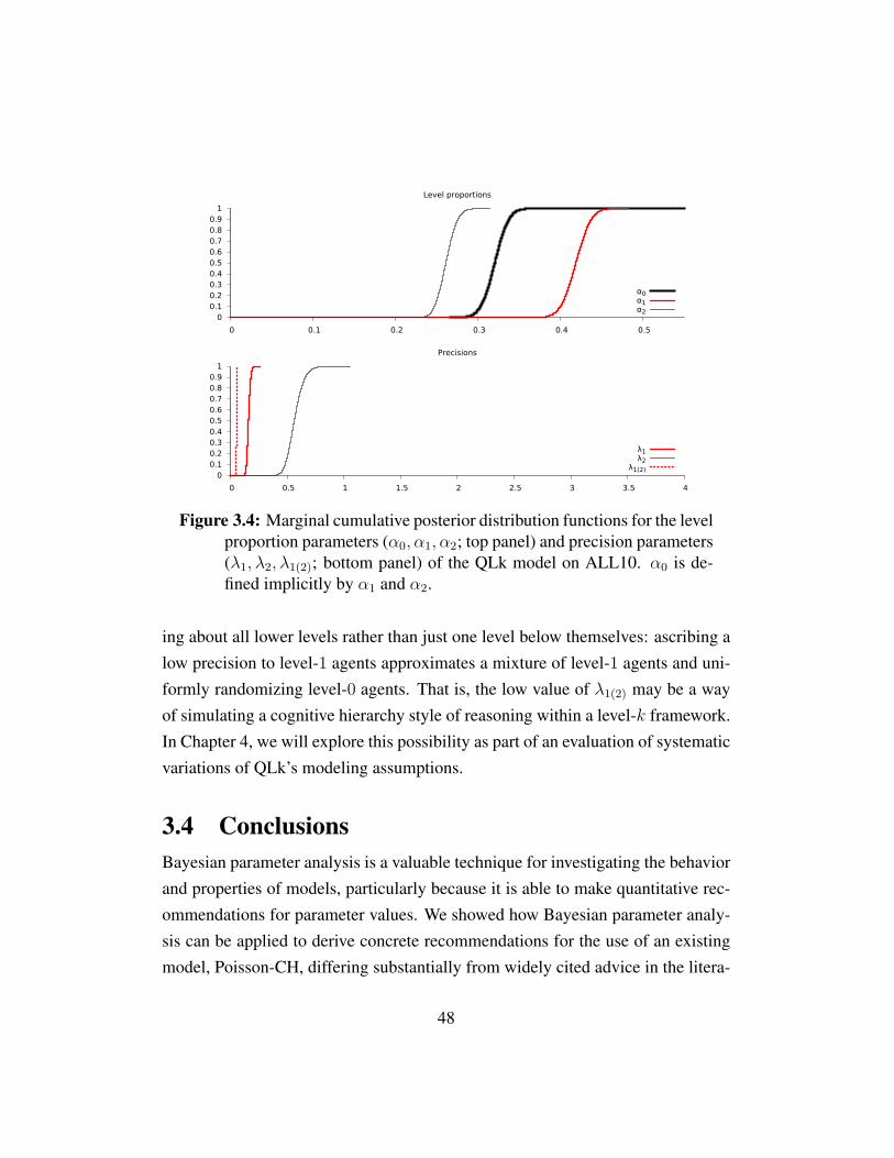
0 0.1 0.2 0.3 0.4 0.5 0.6 0.7 0.8 0.9

1

0 0.1 0.2 0.3 0.4 0.5

Level proportions

α0α1α2

0 0.1 0.2 0.3 0.4 0.5 0.6 0.7 0.8 0.9

1

0 0.5 1 1.5 2 2.5 3 3.5 4

Precisions

λ1λ2

λ1(2)

Figure 3.4: Marginal cumulative posterior distribution functions for the levelproportion parameters (α0, α1, α2; top panel) and precision parameters(λ1, λ2, λ1(2); bottom panel) of the QLk model on ALL10. α0 is de-fined implicitly by α1 and α2.

ing about all lower levels rather than just one level below themselves: ascribing alow precision to level-1 agents approximates a mixture of level-1 agents and uni-formly randomizing level-0 agents. That is, the low value of λ1(2) may be a wayof simulating a cognitive hierarchy style of reasoning within a level-k framework.In Chapter 4, we will explore this possibility as part of an evaluation of systematicvariations of QLk’s modeling assumptions.

3.4 ConclusionsBayesian parameter analysis is a valuable technique for investigating the behaviorand properties of models, particularly because it is able to make quantitative rec-ommendations for parameter values. We showed how Bayesian parameter analy-sis can be applied to derive concrete recommendations for the use of an existingmodel, Poisson-CH, differing substantially from widely cited advice in the litera-

48

ture.Our parameter estimates for all of the iterative models included a substantial

proportion of level-0 agents. The level-0 model is important for predicting thebehavior of all agents in an iterative model; both the level-0 agents themselves,and the higher-level agents whose behavior is grounded in a model of level-0behavior. Motivated by this, we introduce a richer specification of level-0 behaviorin Chapter 5, which allows for significant performance improvements.

49

Chapter 4

Model Variations

QLk incorporates a number of modeling assumptions. In this chapter, we inves-tigate the properties of the QLk model by evaluating the predictive power of afamily of models that systematically vary a set of these assumptions. In the end,we identify a simpler model that dominated QLk on our data.

4.1 ConstructionWe constructed a broad family of models by modifying the QLk model along fourdifferent axes. First, QLk assumes a maximum level of 2; we considered maxi-mum levels of 1 and 3 as well. Second, QLk assumes inhomogeneous precisions

in that it allows each level to have a different precision; we varied this by alsoconsidering homogeneous precision models. Third, QLk allows general precision

beliefs that can differ from lower-level agents’ true precisions; we also constructedmodels that make the simplifying assumption that all agents have accurate pre-

cision beliefs about lower-level agents.1 Finally, in addition to Lk beliefs (whereall other agents are assumed by a level-k agent to be level-(k − 1)), we also con-structed models with CH beliefs (where agents believe that the population con-sists of the true, truncated distribution over the lower levels). We evaluated each

1This is in the same spirit as the simplifying assumption made in cognitive hierarchy modelsthat agents have accurate beliefs about the proportions of lower-level agents.

50

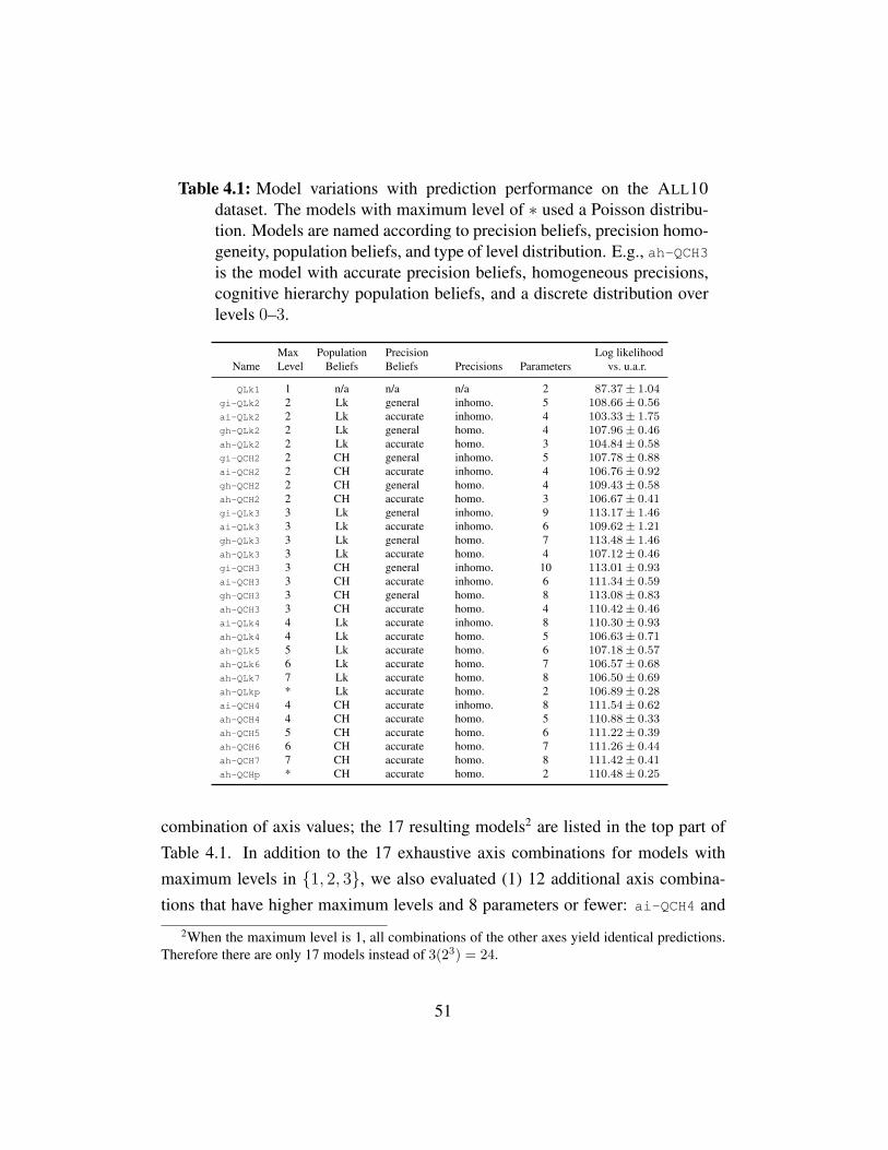
Table 4.1: Model variations with prediction performance on the ALL10dataset. The models with maximum level of ∗ used a Poisson distribu-tion. Models are named according to precision beliefs, precision homo-geneity, population beliefs, and type of level distribution. E.g., ah-QCH3is the model with accurate precision beliefs, homogeneous precisions,cognitive hierarchy population beliefs, and a discrete distribution overlevels 0–3.

NameMaxLevel

PopulationBeliefs

PrecisionBeliefs Precisions Parameters

Log likelihoodvs. u.a.r.

QLk1 1 n/a n/a n/a 2 87.37± 1.04gi-QLk2 2 Lk general inhomo. 5 108.66± 0.56ai-QLk2 2 Lk accurate inhomo. 4 103.33± 1.75gh-QLk2 2 Lk general homo. 4 107.96± 0.46ah-QLk2 2 Lk accurate homo. 3 104.84± 0.58gi-QCH2 2 CH general inhomo. 5 107.78± 0.88ai-QCH2 2 CH accurate inhomo. 4 106.76± 0.92gh-QCH2 2 CH general homo. 4 109.43± 0.58ah-QCH2 2 CH accurate homo. 3 106.67± 0.41gi-QLk3 3 Lk general inhomo. 9 113.17± 1.46ai-QLk3 3 Lk accurate inhomo. 6 109.62± 1.21gh-QLk3 3 Lk general homo. 7 113.48± 1.46ah-QLk3 3 Lk accurate homo. 4 107.12± 0.46gi-QCH3 3 CH general inhomo. 10 113.01± 0.93ai-QCH3 3 CH accurate inhomo. 6 111.34± 0.59gh-QCH3 3 CH general homo. 8 113.08± 0.83ah-QCH3 3 CH accurate homo. 4 110.42± 0.46ai-QLk4 4 Lk accurate inhomo. 8 110.30± 0.93ah-QLk4 4 Lk accurate homo. 5 106.63± 0.71ah-QLk5 5 Lk accurate homo. 6 107.18± 0.57ah-QLk6 6 Lk accurate homo. 7 106.57± 0.68ah-QLk7 7 Lk accurate homo. 8 106.50± 0.69ah-QLkp * Lk accurate homo. 2 106.89± 0.28ai-QCH4 4 CH accurate inhomo. 8 111.54± 0.62ah-QCH4 4 CH accurate homo. 5 110.88± 0.33ah-QCH5 5 CH accurate homo. 6 111.22± 0.39ah-QCH6 6 CH accurate homo. 7 111.26± 0.44ah-QCH7 7 CH accurate homo. 8 111.42± 0.41ah-QCHp * CH accurate homo. 2 110.48± 0.25

combination of axis values; the 17 resulting models2 are listed in the top part ofTable 4.1. In addition to the 17 exhaustive axis combinations for models withmaximum levels in {1, 2, 3}, we also evaluated (1) 12 additional axis combina-tions that have higher maximum levels and 8 parameters or fewer: ai-QCH4 and

2When the maximum level is 1, all combinations of the other axes yield identical predictions.Therefore there are only 17 models instead of 3(23) = 24.

51

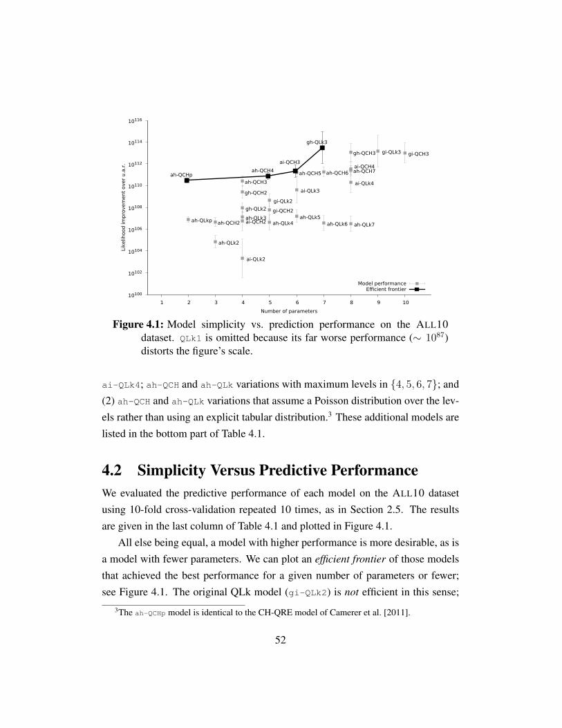
10100

10102

10104

10106

10108

10110

10112

10114

10116

1 2 3 4 5 6 7 8 9 10

Like

lihood

im

pro

vem

ent

over

u.a

.r.

Number of parameters

Model performance

ah-QLkp

ah-QLk2

ah-QCH2

ai-QLk2

ai-QCH2ah-QLk3

gh-QLk2

gh-QCH2

ah-QCH3

ah-QLk4

gi-QCH2

gi-QLk2

ah-QLk5

ai-QLk3

ah-QCH5

ah-QLk6

ah-QCH6

ah-QLk7

ai-QLk4

ah-QCH7ai-QCH4

gh-QCH3 gi-QLk3 gi-QCH3

Efficient frontier

ah-QCHpah-QCH4

ai-QCH3

gh-QLk3

Figure 4.1: Model simplicity vs. prediction performance on the ALL10dataset. QLk1 is omitted because its far worse performance (∼ 1087)distorts the figure’s scale.

ai-QLk4; ah-QCH and ah-QLk variations with maximum levels in {4, 5, 6, 7}; and(2) ah-QCH and ah-QLk variations that assume a Poisson distribution over the lev-els rather than using an explicit tabular distribution.3 These additional models arelisted in the bottom part of Table 4.1.

4.2 Simplicity Versus Predictive PerformanceWe evaluated the predictive performance of each model on the ALL10 datasetusing 10-fold cross-validation repeated 10 times, as in Section 2.5. The resultsare given in the last column of Table 4.1 and plotted in Figure 4.1.

All else being equal, a model with higher performance is more desirable, as isa model with fewer parameters. We can plot an efficient frontier of those modelsthat achieved the best performance for a given number of parameters or fewer;see Figure 4.1. The original QLk model (gi-QLk2) is not efficient in this sense;

3The ah-QCHp model is identical to the CH-QRE model of Camerer et al. [2011].

52

0 0.1 0.2 0.3 0.4 0.5 0.6 0.7 0.8 0.9

1

0 0.1 0.2 0.3 0.4 0.5

Cum

ula

tive p

robabili

ty

λ

ah-qch3ah-qch4

Figure 4.2: Marginal cumulative posterior distributions for the precision pa-rameter (λ) of the ah-QCH3 and ah-QCH4 models on ALL10.

it is dominated by, e.g., ah-QCH3, which has both significantly better predictiveperformance and fewer parameters (because it restricts agents to homogeneousprecisions and accurate beliefs).

There is a striking pattern among the efficient models with 6 parameters orfewer: every such model has accurate precision beliefs, cognitive hierarchy pop-ulation beliefs, and, with the exception of ai-QCH3, homogeneous precisions.Furthermore, ai-QCH3’s performance was not significantly better than that ofah-QCH5, which did have homogeneous precisions. This suggests that the mostparsimonious way to model human behavior in normal-form games is to use amodel of this form.

Adding flexibility by modeling general beliefs about precisions did improveperformance; the four best-performing models all incorporated general precisionbeliefs. However, these models also had much larger variance in their predictionperformance on the test set. This may indicate that the models are overly flexible,and hence prone to overfitting.

53

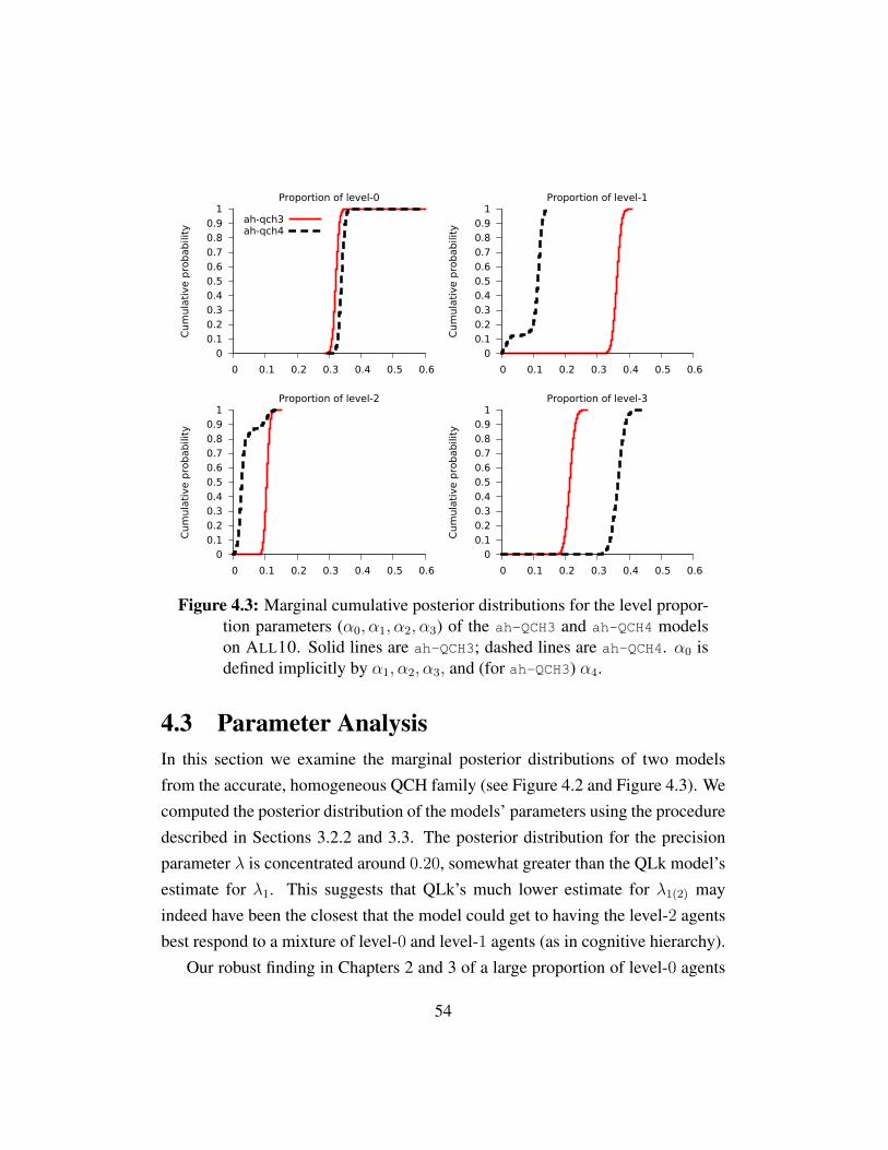
0 0.1 0.2

0.3 0.4 0.5 0.6 0.7

0.8 0.9

1

0 0.1 0.2 0.3 0.4 0.5 0.6

Cum

ula

tive p

robabili

tyProportion of level-0

ah-qch3ah-qch4

0 0.1 0.2

0.3 0.4 0.5 0.6 0.7

0.8 0.9

1

0 0.1 0.2 0.3 0.4 0.5 0.6

Cum

ula

tive p

robabili

ty

Proportion of level-1

0 0.1

0.2 0.3 0.4

0.5 0.6 0.7 0.8

0.9 1

0 0.1 0.2 0.3 0.4 0.5 0.6

Cum

ula

tive p

robabili

ty

Proportion of level-2

0 0.1

0.2 0.3 0.4

0.5 0.6 0.7 0.8

0.9 1

0 0.1 0.2 0.3 0.4 0.5 0.6

Cum

ula

tive p

robabili

ty

Proportion of level-3

Figure 4.3: Marginal cumulative posterior distributions for the level propor-tion parameters (α0, α1, α2, α3) of the ah-QCH3 and ah-QCH4 modelson ALL10. Solid lines are ah-QCH3; dashed lines are ah-QCH4. α0 isdefined implicitly by α1, α2, α3, and (for ah-QCH3) α4.

4.3 Parameter AnalysisIn this section we examine the marginal posterior distributions of two modelsfrom the accurate, homogeneous QCH family (see Figure 4.2 and Figure 4.3). Wecomputed the posterior distribution of the models’ parameters using the proceduredescribed in Sections 3.2.2 and 3.3. The posterior distribution for the precisionparameter λ is concentrated around 0.20, somewhat greater than the QLk model’sestimate for λ1. This suggests that QLk’s much lower estimate for λ1(2) mayindeed have been the closest that the model could get to having the level-2 agentsbest respond to a mixture of level-0 and level-1 agents (as in cognitive hierarchy).

Our robust finding in Chapters 2 and 3 of a large proportion of level-0 agents

54

is confirmed by these models as well. Indeed, the number of level-0 agents isnearly the only point of close agreement between the two models with respect tothe distribution of levels.

4.4 Spike-PoissonWe saw evidence in Section 4.2 that the ah-QCH family of models had good perfor-mance, with relatively low variance. Another group of general precision modelshad higher performance, but higher variance suggestive of overfitting. In Sec-tion 4.3, we saw that the ah-QCH family broadly agreed on a proportion of level-0agents of about 0.30, but ascribed varying proportions to the other levels. It seemsthat the data argue very consistently for a particular proportion of level-0 agents,and less consistently for the proportions of other levels. At the same time, we sawin Section 4.2 that performance improved within the ah-QCH family as the numberof modeled levels increased.

In this section, we describe a low-parameter model that specifies the propor-tion of agents using a mixture of a deterministic fraction of level-0 agents and astandard Poisson distribution. This allows for the precise targeting of the level-0proportion, while also allowing a single parameter to specify the proportions ofhigher levels. We refer to this mixture as a Spike-Poisson distribution. Because wewill end up recommending its use, we define the full Spike-Poisson QCH modelhere.

Definition 7 (Spike-Poisson Quantal Cognitive Hierarchy (QCH) model). LetπSPi,m ∈ Π(Ai) be the distribution over actions predicted for an agent i with levelm by the Spike-Poisson QCH model. Let

f(m) =

ε+ (1− ε)Poisson(m; τ) if m = 0,

(1− ε)Poisson(m; τ) otherwise.

55

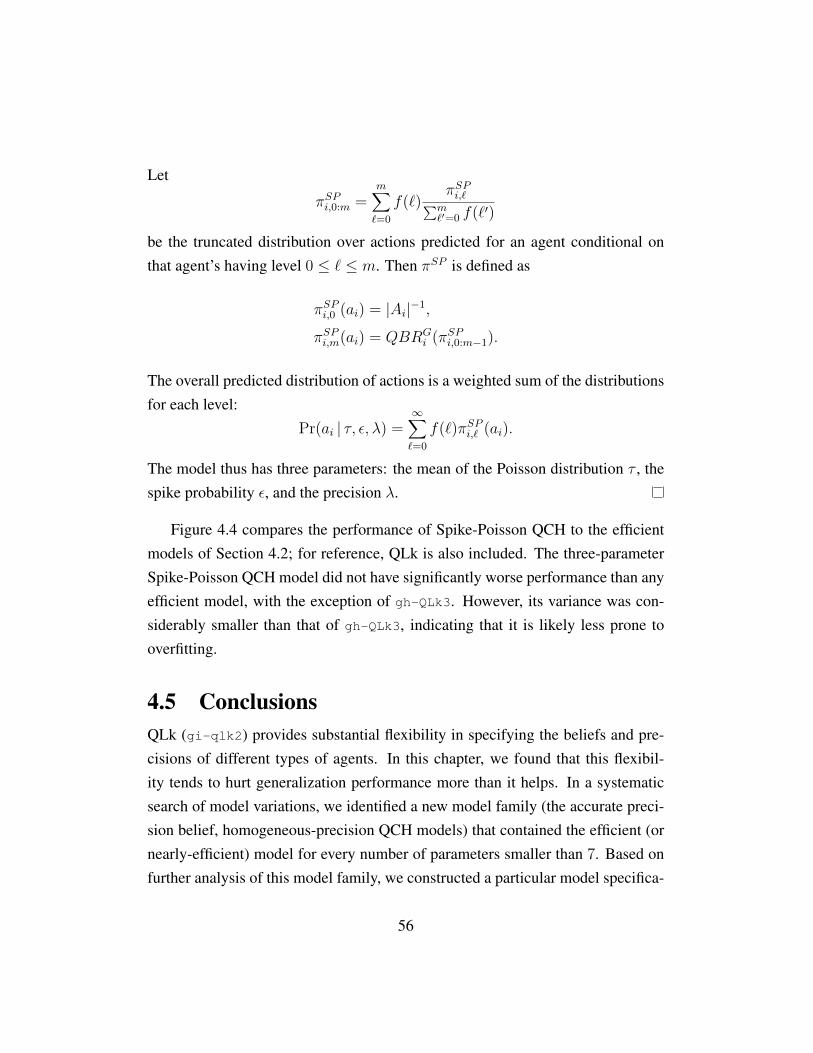
Let

πSPi,0:m =m∑`=0

f(`)πSPi,`∑m

`′=0 f(`′)

be the truncated distribution over actions predicted for an agent conditional onthat agent’s having level 0 ≤ ` ≤ m. Then πSP is defined as

πSPi,0 (ai) = |Ai|−1,

πSPi,m(ai) = QBRGi (πSPi,0:m−1).

The overall predicted distribution of actions is a weighted sum of the distributionsfor each level:

Pr(ai | τ, ε, λ) =∞∑`=0

f(`)πSPi,` (ai).

The model thus has three parameters: the mean of the Poisson distribution τ , thespike probability ε, and the precision λ.

Figure 4.4 compares the performance of Spike-Poisson QCH to the efficientmodels of Section 4.2; for reference, QLk is also included. The three-parameterSpike-Poisson QCH model did not have significantly worse performance than anyefficient model, with the exception of gh-QLk3. However, its variance was con-siderably smaller than that of gh-QLk3, indicating that it is likely less prone tooverfitting.

4.5 ConclusionsQLk (gi-qlk2) provides substantial flexibility in specifying the beliefs and pre-cisions of different types of agents. In this chapter, we found that this flexibil-ity tends to hurt generalization performance more than it helps. In a systematicsearch of model variations, we identified a new model family (the accurate preci-sion belief, homogeneous-precision QCH models) that contained the efficient (ornearly-efficient) model for every number of parameters smaller than 7. Based onfurther analysis of this model family, we constructed a particular model specifica-

56

10108

10109

10110

10111

10112

10113

10114

10115

1 2 3 4 5 6 7 8 9 10

Like

lihood

im

pro

vem

ent

over

u.a

.r.

Number of parameters

Model performance

ah-QCHp

ah-QCH-sp ah-QCH4

gi-QLk2

ai-QCH3

gh-QLk3

Figure 4.4: Model simplicity (number of parameters) versus prediction per-formance on the ALL10 dataset, comparing the efficient models fromSection 4.2, QLk, and and Spike-Poisson QCH.

tion (Spike-Poisson QCH) which offers excellent generalization performance inspite of having only three parameters.

In Chapter 5, we will build further on this model, constructing a model thatpredicts better than even gh-QLk3, while still having fewer parameters and lowervariance. We thus recommend the use of Spike-Poisson by researchers wanting topredict human play in (unrepeated) normal-form games, in conjunction with thelevel-0 extensions of Chapter 5.

57

Chapter 5

Models of Level-0 Behavior

5.1 IntroductionIn quantal cognitive hierarchy models, such as the Spike-Poisson QCH modelfrom Chapter 4, agents do not reason arbitrarily deeply about their opponents’beliefs about beliefs about beliefs. Instead, they start from a simple nonstrategicstrategy1 (the level-0 behavior), and then reason for some fixed number of itera-tions about responses to that strategy (e.g., a level-2 agent quantally best respondsto the combined behaviors of level-1 and level-0 agents).

Thus, in order to make use of a quantal cognitive hierarchy model one mustfirst commit to a specification of level-0 behavior. Indeed, this is true of iterativemodels in general, such as cognitive hierarchy [Camerer et al., 2004] and level-k[Stahl and Wilson, 1994; Nagel, 1995; Costa-Gomes et al., 2001]. It is importantto get this specification right, for two reasons. First, there is growing evidencethat a substantial fraction of human players do act nonstrategically [Burchardiand Penczynski, 2012; Chapter 3 of this dissertation]. Second, a level-0 modelalso drives predictions that are made about strategic agents: higher-level agents

1In this work, we refer to agents that form explicit beliefs about the behavior of other agentsas “strategic,” and agents that do not reason about other agents in this way as “nonstrategic”.Nonstrategic should not be taken as a synonym for unsophisticated or thoughtless. Some of thelevel-0 behavior that we describe below is rather sophisticated.

58

are assumed to act by responding strategically to lower-level agents’ behavior.Almost all work in the literature that uses iterative models adopts the spec-

ification that level-0 agents play a uniform distribution over actions. (In Sec-tion 5.4 we discuss the few exceptions of which we are aware, each of which isbased on an explicitly encoded intuition about a specific setting of interest.) Theuniform-distribution approach has the advantage that it does not require insightinto a game’s structure, and hence can be applied to any game. However, in manygames it is not plausible that an agent would choose an action uniformly at ran-dom, nor that any other agent would expect them to do so. For example, considera dominated action that always yields very low payoffs for all players.

In this chapter we consider the question of how to do better. Specifically, weinvestigate general rules that can be used to induce a level-0 specification from thenormal-form description of an arbitrary game.

5.2 Level-0 ModelIn this section we present the components from which we will construct modelsfor computing level-0 distributions of play. We first describe features computedfor each of an agent’s actions, followed by options for combining feature valuesto obtain a level-0 prediction.

5.2.1 Level-0 FeaturesMost applications of iterative models specify that level-0 agents choose their ac-tions uniformly, thus implicitly identifying nonstrategic behavior with uniformrandomization. The core idea of this chapter is that nonstrategic behavior neednot be uniform. How then might a nonstrategic agent behave? We argue thatagents consider simple rules (features) that recommend one or more actions, togreater or lesser degrees. We consider both binary features with range {0, 1} andreal-valued features with range R+.

To be eligible for inclusion in our level-0 specification, we require that fea-

59

tures not depend on beliefs about how other agents will attempt to maximize theirown utility functions. E.g., the maxmax payoff feature (see below) could be in-terpreted as a belief that the other agents will act in such a way that the level-0agent can maximize its own payoff; however, this belief does not take the otheragents’ utility function into account at all. The minmin unfairness feature (seebelow) could be interpreted as a belief that the other agents will act to minimizeunfairness; however, it does not model the other agents as attempting to maximizetheir own utility at all.

We restrict our attention to features that can be computed directly from the nor-mal form of the game, and which do not depend on presentation details such as theunits in which payoffs are expressed or the order in which actions are presented.This allows for more accurate analysis of strategic models, even when details ofpresentation are unknown or not yet known. We do not claim that the features thatwe investigated comprise an exhaustive list of factors that could influence non-strategic agents’ actions. In Chapter 6, we will consider a more automated butless interpretable procedure for learning nonstrategic features.

For each feature, we briefly describe its motivation and then formally defineit. Many of our features have been investigated in both the classical and behav-ioral game theory literature in other contexts. In particular, the maxmax payoff,maxmin payoff, and maxmax welfare features correspond to the Optimistic, Pes-

simistic, and Altruistic nonstrategic types in Costa-Gomes et al. [2001]. Otherfeatures, such as the max-symmetric feature, were influenced by introspectionabout paradigmatic games such as the Traveler’s Dilemma.

For each feature, we define both a binary version and a real-valued version.Unlike a binary feature, where a criterion must be maximized in order to be rec-ommended, with a real-valued feature an action will be recommended to the de-

gree that it maximizes a criterion. This addresses the intuition that two very highpayoff actions may both be attractive, even if one offers marginally higher payoffthan the other.

Some real-valued features represent quantities that an agent would wish to

60

minimize, rather than maximizing. We apply the inv transformation to these fea-tures, where inv is defined differently depending upon how features will be com-bined. If feature values will be combined linearly, then inv(x) = 1/x. If featurevalues will be combined with a logit function, then inv(x) = −x.

Maxmin payoff. A maxmin action for agent i is the action with the best worst-case guarantee. That is,

fmaxmin(ai) =

1 if ai ∈ arg maxa′i∈Aimina−i∈A−i

ui(a′i, a−i),

0 otherwise.

This is the safest single action to play against a hostile agent.2 The real-valuedversion of this feature returns the worst-case payoff for an action:

fmin(ai) = mina−i∈A−i

ui(ai, a−i).

Maxmax payoff. In contrast, a maxmax action for agent i is the action with thebest best case. That is,

fmaxmax(ai) =

1 if ai ∈ arg maxa′i∈Aimaxa−i∈A−i

ui(a′i, a−i),

0 otherwise.

An agent who aims to maximize his possible payoff will play a maxmax action.The real-valued version of this feature returns the best-case payoff for an action:

fmax(ai) = maxa−i∈A−i

ui(ai, a−i).

2Often, a mixed strategy will be safer still against a hostile agent. However, in this applicationwe are not actually trying to find a safest strategy for the agent. Rather, we are trying to specifyfeatures of individual actions that might make them attractive to nonstrategic agents.

61

Minimax regret. Savage [1951] proposed the minimax regret criterion for mak-ing decisions in the absence of probabilistic beliefs. In a game theoretic context,it works as follows. For each action profile, an agent has a possible regret: howmuch more utility could the agent have gained by playing the best response to theother agents’ actions? Each of the agent’s actions is therefore associated with avector of possible regrets, one for each possible profile of the other agents’ ac-tions. A minimax regret action is an action whose maximum regret (in the vectorof possible regrets) is minimal. That is, if

r(ai, a−i) = ui(ai, a−i)− maxa∗i∈Ai

ui(a∗i , a−i)

is the regret of agent i in action profile (ai, a−i), then

fmmr(ai) =

1 if ai ∈ arg mina′i∈Aimaxa−i∈A−i

r(ai, a−i),

0 otherwise.

The real-valued version of this feature returns the worst-case regret for playing anaction:

fmr(ai) = inv[

maxa−i∈A−i

r(ai, a−i)].

Higher max regret is less desirable than lower max regret, explaining our use ofthe inv transformation.

Minmin unfairness. Concern for the fairness of outcomes is a common featureof human play in strategic situations, as has been confirmed in multiple behav-ioral studies, most famously in the Ultimatum game [Thaler, 1988; Camerer andThaler, 1995]. Let the unfairness of an action profile be the difference betweenthe maximum and minimum payoffs among the agents under that action profile:

d(a) = maxi,j∈N

ui(a)− uj(a).

62

Then a fair outcome minimizes this difference in utilities. The minmin unfairness

feature selects every action which is part of a minimally unfair action profile.

f fair(ai) =

1 if ai ∈ arg mina′i∈Aimina−i∈A−i

d(a′i, a−i),

0 otherwise.

The real-valued version of this feature returns the minimum unfairness that couldresult from playing a given action:

f unfair(ai) = inv[

mina−i∈A−i

d(ai, a−i)].

Unfairness is a quantity to be minimized, so we apply the inv transformation.

Max symmetric. People often reason about what would happen if the other agentacted as they did.3 A max-symmetric action is simply the best such action:

fmaxsymm(ai) =

1 if ai ∈ arg maxa′i∈Aiu(a′i, . . . , a′i),

0 otherwise.

The real-valued version of this feature returns the symmetric payoff of an action:

f symm(ai) = u(ai, . . . , ai).

Maxmax welfare. Finally, one reason that a nonstrategic agent might find anaction profile desirable is that it produces the best overall benefit to the pair ofagents. The maxmax welfare feature selects every action that is part of some

3This is a concept that only applies to symmetric games, in which agents have identical actionsets, and each agent’s payoff matrix is the transpose of the other.

63

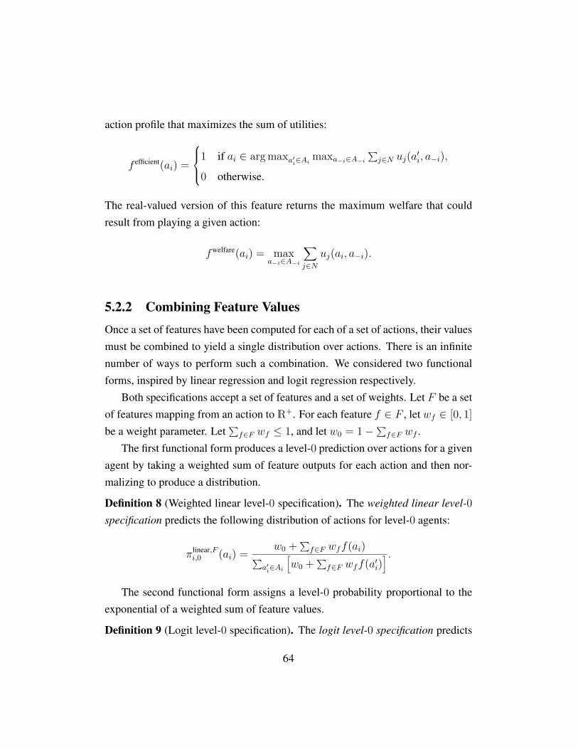
action profile that maximizes the sum of utilities:

f efficient(ai) =

1 if ai ∈ arg maxa′i∈Aimaxa−i∈A−i

∑j∈N uj(a′i, a−i),

0 otherwise.

The real-valued version of this feature returns the maximum welfare that couldresult from playing a given action:

fwelfare(ai) = maxa−i∈A−i

∑j∈N

uj(ai, a−i).

5.2.2 Combining Feature ValuesOnce a set of features have been computed for each of a set of actions, their valuesmust be combined to yield a single distribution over actions. There is an infinitenumber of ways to perform such a combination. We considered two functionalforms, inspired by linear regression and logit regression respectively.

Both specifications accept a set of features and a set of weights. Let F be a setof features mapping from an action to R+. For each feature f ∈ F , let wf ∈ [0, 1]be a weight parameter. Let

∑f∈F wf ≤ 1, and let w0 = 1−∑f∈F wf .

The first functional form produces a level-0 prediction over actions for a givenagent by taking a weighted sum of feature outputs for each action and then nor-malizing to produce a distribution.

Definition 8 (Weighted linear level-0 specification). The weighted linear level-0specification predicts the following distribution of actions for level-0 agents:

πlinear,Fi,0 (ai) =

w0 +∑f∈F wff(ai)∑

a′i∈Ai

[w0 +∑

f∈F wff(a′i)] .

The second functional form assigns a level-0 probability proportional to theexponential of a weighted sum of feature values.

Definition 9 (Logit level-0 specification). The logit level-0 specification predicts

64

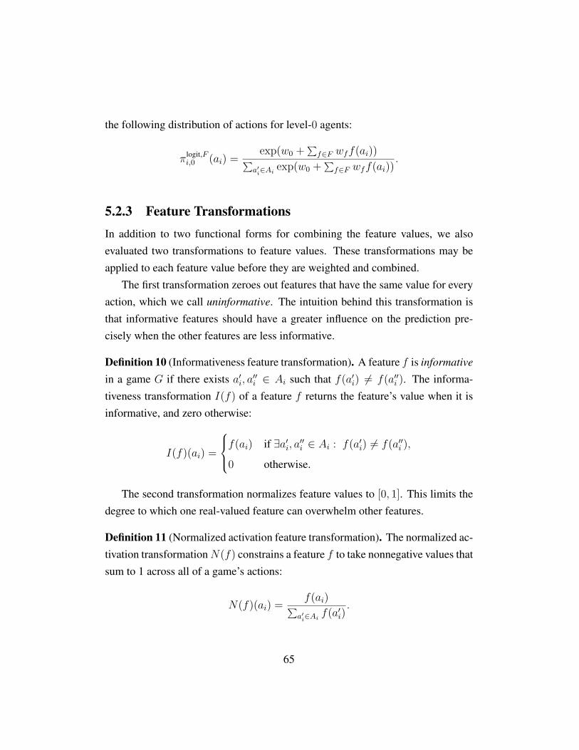
the following distribution of actions for level-0 agents:

πlogit,Fi,0 (ai) =

exp(w0 +∑f∈F wff(ai))∑

a′i∈Aiexp(w0 +∑

f∈F wff(ai)).

5.2.3 Feature TransformationsIn addition to two functional forms for combining the feature values, we alsoevaluated two transformations to feature values. These transformations may beapplied to each feature value before they are weighted and combined.

The first transformation zeroes out features that have the same value for everyaction, which we call uninformative. The intuition behind this transformation isthat informative features should have a greater influence on the prediction pre-cisely when the other features are less informative.

Definition 10 (Informativeness feature transformation). A feature f is informative

in a game G if there exists a′i, a′′i ∈ Ai such that f(a′i) 6= f(a′′i ). The informa-

tiveness transformation I(f) of a feature f returns the feature’s value when it isinformative, and zero otherwise:

I(f)(ai) =

f(ai) if ∃a′i, a′′i ∈ Ai : f(a′i) 6= f(a′′i ),

0 otherwise.

The second transformation normalizes feature values to [0, 1]. This limits thedegree to which one real-valued feature can overwhelm other features.

Definition 11 (Normalized activation feature transformation). The normalized ac-tivation transformationN(f) constrains a feature f to take nonnegative values thatsum to 1 across all of a game’s actions:

N(f)(ai) = f(ai)∑a′i∈Ai

f(a′i).

65

5.3 Model SelectionWe took two approaches to constructing a model from the candidate features,functional forms, and transformations described in the previous section. First, weperformed forward selection of binary features, using a linear functional form andinformativeness transformation. We chose this functional form based on a man-ual evaluation we performed in the conference version of this chapter [Wrightand Leyton-Brown, 2014], in which a linear functional form and normalized-activation- and informativeness-transformed binary features yielded good perfor-mance. Second, we performed Bayesian optimization to automatically evaluatecombinations from the full set of candidate features, functional forms, and trans-formations.

5.3.1 Forward SelectionWe performed forward selection using the following procedure. We evaluatedthe test performance of the Spike-Poisson QCH model, extended by a linear,normalized-activation- and informativeness-transformed level-0 model using ev-ery one- and two-element subset of the binary features from Section 5.2.1. Thebest such model used the minmin unfairness and max symmetric features. Wethen evaluated every combination of features that contained those two features.The results are shown in Figure 5.1.

The best performing linear model found by forward selection contained fourfeatures: maxmax payoff, maxmin payoff, minmin unfairness, and max symmet-ric. We will refer to this model henceforth as linear4. Adding further featuresdid not improve prediction performance. Figure 5.2 shows the training and testperformance for the best-performing model at each number of features. Noticethat the training performance increased with every additional feature, whereasafter the four-feature model the test performance decreased. This confirms thatoverfitting was the cause of the performance decrease.4

4It might seem obvious that a drop in test performance for more general models must im-ply overfitting. However, it could also indicate underfitting, where we simply do a worse job of

66

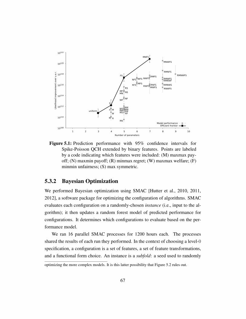
10108

10110

10112

10114

10116

10118

10120

10122

1 2 3 4 5 6 7 8 9 10

Like

lihood

im

pro

vem

ent

over

u.a

.r.

Number of parameters

Model performanceEfficient frontier

uniform

RN

W

F M

S

RN

RFMS RWRM MWWSNW

WFNF

MN NSMFRS

FS

RFSMFS

NFS WFS

MWFSRWFS RNFS

NWFSRMFS

MNFS

RNWFS

RMNWS

RMNWFRMWFS

RMNFS

MNWFS

RMNWFS

Figure 5.1: Prediction performance with 95% confidence intervals forSpike-Poisson QCH extended by binary features. Points are labeledby a code indicating which features were included: (M) maxmax pay-off; (N) maxmin payoff; (R) minmax regret; (W) maxmax welfare; (F)minmin unfairness; (S) max symmetric.

5.3.2 Bayesian OptimizationWe performed Bayesian optimization using SMAC [Hutter et al., 2010, 2011,2012], a software package for optimizing the configuration of algorithms. SMACevaluates each configuration on a randomly-chosen instance (i.e., input to the al-gorithm); it then updates a random forest model of predicted performance forconfigurations. It determines which configurations to evaluate based on the per-formance model.

We ran 16 parallel SMAC processes for 1200 hours each. The processesshared the results of each run they performed. In the context of choosing a level-0specification, a configuration is a set of features, a set of feature transformations,and a functional form choice. An instance is a subfold: a seed used to randomly

optimizing the more complex models. It is this latter possibility that Figure 5.2 rules out.

67

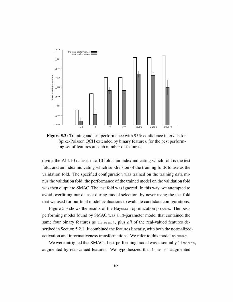
10110

10112

10114

10116

10118

10120

10122

10124

10126

unif S FS EFS MNFS MNEFS RMNEFS

Like

lihood

im

pro

vem

ent

training performancetest performance

Figure 5.2: Training and test performance with 95% confidence intervals forSpike-Poisson QCH extended by binary features, for the best perform-ing set of features at each number of features.

divide the ALL10 dataset into 10 folds; an index indicating which fold is the testfold; and an index indicating which subdivision of the training folds to use as thevalidation fold. The specified configuration was trained on the training data mi-nus the validation fold; the performance of the trained model on the validation foldwas then output to SMAC. The test fold was ignored. In this way, we attempted toavoid overfitting our dataset during model selection, by never using the test foldthat we used for our final model evaluations to evaluate candidate configurations.

Figure 5.3 shows the results of the Bayesian optimization process. The best-performing model found by SMAC was a 13-parameter model that contained thesame four binary features as linear4, plus all of the real-valued features de-scribed in Section 5.2.1. It combined the features linearly, with both the normalized-activation and informativeness transformations. We refer to this model as smac.

We were intrigued that SMAC’s best-performing model was essentially linear4,augmented by real-valued features. We hypothesized that linear4 augmented

68

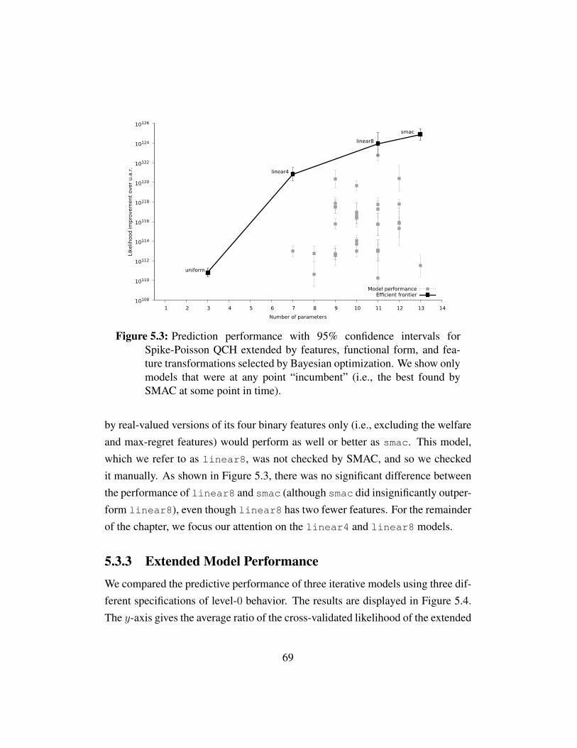
10108

10110

10112

10114

10116

10118

10120

10122

10124

10126

1 2 3 4 5 6 7 8 9 10 11 12 13 14

Like

lihood

im

pro

vem

ent

over

u.a

.r.

Number of parameters

Model performance

uniform

linear4

linear8

smac

Efficient frontier

Figure 5.3: Prediction performance with 95% confidence intervals forSpike-Poisson QCH extended by features, functional form, and fea-ture transformations selected by Bayesian optimization. We show onlymodels that were at any point “incumbent” (i.e., the best found bySMAC at some point in time).

by real-valued versions of its four binary features only (i.e., excluding the welfareand max-regret features) would perform as well or better as smac. This model,which we refer to as linear8, was not checked by SMAC, and so we checkedit manually. As shown in Figure 5.3, there was no significant difference betweenthe performance of linear8 and smac (although smac did insignificantly outper-form linear8), even though linear8 has two fewer features. For the remainderof the chapter, we focus our attention on the linear4 and linear8 models.

5.3.3 Extended Model PerformanceWe compared the predictive performance of three iterative models using three dif-ferent specifications of level-0 behavior. The results are displayed in Figure 5.4.The y-axis gives the average ratio of the cross-validated likelihood of the extended

69

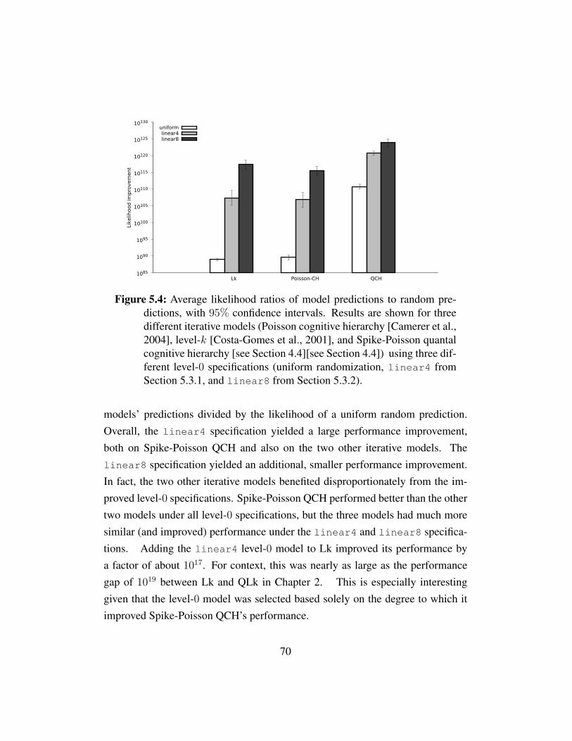
1085

1090

1095

10100

10105

10110

10115

10120

10125

10130

Lk Poisson-CH QCH

Like

lihood

im

pro

vem

ent

uniformlinear4linear8

Figure 5.4: Average likelihood ratios of model predictions to random pre-dictions, with 95% confidence intervals. Results are shown for threedifferent iterative models (Poisson cognitive hierarchy [Camerer et al.,2004], level-k [Costa-Gomes et al., 2001], and Spike-Poisson quantalcognitive hierarchy [see Section 4.4][see Section 4.4]) using three dif-ferent level-0 specifications (uniform randomization, linear4 fromSection 5.3.1, and linear8 from Section 5.3.2).

models’ predictions divided by the likelihood of a uniform random prediction.Overall, the linear4 specification yielded a large performance improvement,both on Spike-Poisson QCH and also on the two other iterative models. Thelinear8 specification yielded an additional, smaller performance improvement.In fact, the two other iterative models benefited disproportionately from the im-proved level-0 specifications. Spike-Poisson QCH performed better than the othertwo models under all level-0 specifications, but the three models had much moresimilar (and improved) performance under the linear4 and linear8 specifica-tions. Adding the linear4 level-0 model to Lk improved its performance bya factor of about 1017. For context, this was nearly as large as the performancegap of 1019 between Lk and QLk in Chapter 2. This is especially interestinggiven that the level-0 model was selected based solely on the degree to which itimproved Spike-Poisson QCH’s performance.

70

0 0.1 0.2

0.3 0.4 0.5 0.6 0.7

0.8 0.9

1

0 0.1 0.2 0.3 0.4 0.5 0.6 0.7

Cum

ula

tive p

robabili

tyProportion of level-0

linear8linear4

uniform

0 0.1 0.2

0.3 0.4 0.5 0.6 0.7

0.8 0.9

1

0 0.1 0.2 0.3 0.4 0.5 0.6 0.7

Cum

ula

tive p

robabili

ty

Proportion of level-1

0 0.1

0.2 0.3 0.4

0.5 0.6 0.7 0.8

0.9 1

0 0.1 0.2 0.3 0.4 0.5 0.6 0.7

Cum

ula

tive p

robabili

ty

Proportion of level-2

0 0.1

0.2 0.3 0.4

0.5 0.6 0.7 0.8

0.9 1

0 0.1 0.2 0.3 0.4 0.5 0.6 0.7

Cum

ula

tive p

robabili

ty

Proportion of level-3

Figure 5.5: Marginal cumulative posterior distributions of levels of reason-ing in the ALL10 dataset, for Spike-Poisson QCH with linear8,linear4, and uniform specifications.

5.3.4 Parameter AnalysisWe now examine and interpret the posterior distributions for some of the parame-ters of the Spike-Poisson model combined with the linear4 and linear8 level-0 specifications, following the methodology of Section 3.2.2.

Figure 5.5 shows the marginal posterior distribution for each level in the pop-ulation (up to level 3), for each of the linear4, linear8, and uniform specifica-tions. We noticed two effects. First, the posterior distribution of level-0 and level-2 agents was essentially identical under the uniform and linear4 specifications,with medians of 0.37. We found this surprising, since the level-0 agents behavevery differently under the two specifications. In contrast, the posterior distribution

71

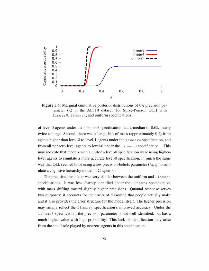
0 0.1 0.2 0.3 0.4 0.5 0.6 0.7 0.8 0.9

1

0 0.2 0.4 0.6 0.8 1

Cum

ula

tive p

robabili

ty

λ

linear8linear4

uniform

Figure 5.6: Marginal cumulative posterior distributions of the precision pa-rameter (λ) in the ALL10 dataset, for Spike-Poisson QCH withlinear8, linear4, and uniform specifications.

of level-0 agents under the linear8 specification had a median of 0.65, nearlytwice as large. Second, there was a large shift of mass (approximately 0.2) fromagents higher than level-3 to level-1 agents under the linear4 specification, andfrom all nonzero-level agents to level-0 under the linear8 specification. Thismay indicate that models with a uniform level-0 specification were using higher-level agents to simulate a more accurate level-0 specification, in much the sameway that QLk seemed to be using a low precision-beliefs parameter (λ1(2)) to sim-ulate a cognitive hierarchy model in Chapter 3.

The precision parameter was very similar between the uniform and linear4

specifications. It was less sharply identified under the linear4 specification,with mass shifting toward slightly higher precisions. Quantal response servestwo purposes: it accounts for the errors of reasoning that people actually makeand it also provides the error structure for the model itself. The higher precisionmay simply reflect the linear4 specification’s improved accuracy. Under thelinear8 specification, the precision parameter is not well identified, but has amuch higher value with high probability. This lack of identification may arisefrom the small role played by nonzero agents in this specification.

72

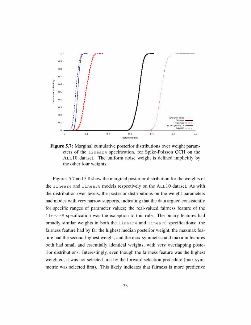
0

0.1

0.2

0.3

0.4

0.5

0.6

0.7

0.8

0.9

1

0 0.1 0.2 0.3 0.4 0.5 0.6

cum

ula

tive p

robab

ility

feature weight

uniform noisefairness

maxmaxmax-symmetric

maxmin

Figure 5.7: Marginal cumulative posterior distributions over weight param-eters of the linear4 specification, for Spike-Poisson QCH on theALL10 dataset. The uniform noise weight is defined implicitly bythe other four weights.

Figures 5.7 and 5.8 show the marginal posterior distribution for the weights ofthe linear4 and linear8 models respectively on the ALL10 dataset. As withthe distribution over levels, the posterior distributions on the weight parametershad modes with very narrow supports, indicating that the data argued consistentlyfor specific ranges of parameter values; the real-valued fairness feature of thelinear8 specification was the exception to this rule. The binary features hadbroadly similar weights in both the linear4 and linear8 specifications: thefairness feature had by far the highest median posterior weight, the maxmax fea-ture had the second-highest weight, and the max-symmetric and maxmin featuresboth had small and essentially identical weights, with very overlapping poste-rior distributions. Interestingly, even though the fairness feature was the highestweighted, it was not selected first by the forward selection procedure (max sym-metric was selected first). This likely indicates that fairness is more predictive

73

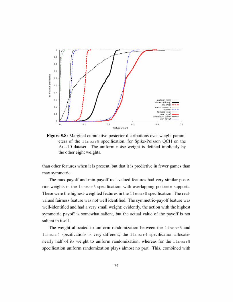
0

0.1

0.2

0.3

0.4

0.5

0.6

0.7

0.8

0.9

1

0 0.1 0.2 0.3 0.4 0.5

cum

ula

tive p

robab

ility

feature weight

uniform noisefairness (binary)

maxmaxmax-symmetric

maxminfairness (real)

max payoffsymmetric payoff

min payoff

Figure 5.8: Marginal cumulative posterior distributions over weight param-eters of the linear8 specification, for Spike-Poisson QCH on theALL10 dataset. The uniform noise weight is defined implicitly bythe other eight weights.

than other features when it is present, but that it is predictive in fewer games thanmax symmetric.

The max-payoff and min-payoff real-valued features had very similar poste-rior weights in the linear8 specification, with overlapping posterior supports.These were the highest-weighted features in the linear8 specification. The real-valued fairness feature was not well identified. The symmetric-payoff feature waswell-identified and had a very small weight; evidently, the action with the highestsymmetric payoff is somewhat salient, but the actual value of the payoff is notsalient in itself.

The weight allocated to uniform randomization between the linear8 andlinear4 specifications is very different; the linear4 specification allocatesnearly half of its weight to uniform randomization, whereas for the linear8

specification uniform randomization plays almost no part. This, combined with

74

the strong similarity in the weighting of binary features between the two specifi-cations, suggests that the real-valued features (especially the max and min payofffeatures) are playing a genuine role in reducing uncertainty.

5.4 Related WorkAlmost every study that employs iterative reasoning models of either the level-k or cognitive hierarchy types assumes a uniform distribution of play for level-0agents. However, there are a few exceptions. Crawford and Iriberri [2007b] spec-ified truth-telling as the single salient action in first-price auctions. Crawford andIriberri [2007a] manually designated certain actions as “salient” (based on visualfeatures such as “leftmost”) in a hide-and-seek game. They then estimated aniterative model with a level-0 specification in which level-0 agents play salientactions, with the strengths of each action’s salience estimated under the assump-tion that no agent truly plays a level-0 distribution. Arad and Rubinstein [2009]specified a single action of reinforcing all battlefields equally in a Colonel Blottogame as the sole level-0 action. Arad and Rubinstein [2012] specified the highestpossible request as the level-0 action in a money-request game where players re-ceive the amount of money they request, but also receive a relatively large bonusfor requesting exactly 1 shekel less than the other player. Arad [2012] manuallyspecified two “anchor” strategies for a Colonel Blotto-like game in which playerssimultaneously assign four representatives to four separate contests in order of therepresentatives’ ability.

In spite of the crucial dependence of iterative models upon the specificationof the level-0 distribution, few studies have empirically investigated level-0 play.Agranov et al. [2010] incentivized subjects to choose an action quickly (and thento revise it after thinking) by imposing a randomized time limit when playing thebeauty-contest game of Nagel [1995]. They hypothesized that early actions repre-sent level-0 choices and that later actions represent higher-level choices. Based onthis assumption, they found that level-0 behavior did not differ significantly froma uniform distribution. In contrast, Burchardi and Penczynski [2012] incentivized

75

players to reveal their reasoning by allowing a one-time simultaneous exchangeof messages between teammates playing a beauty-contest game. Teams of twosimultaneously sent each other a single message containing arguments in favor ofa given action, and then simultaneously chose an action, with the team’s actionbeing chosen randomly from the two choices. Burchardi and Penczynski thenclassified each argument according to level of reasoning, and extracted the level-0behavior from both level-0 and higher-level arguments. They found that level-0play was significantly different from uniform. Intriguingly, they also found thatthe level-0 behavior hypothesized by higher-level players was very similar to thelevel-0 behavior that was actually proposed.

Hargreaves Heap et al. [2014] evaluate the transferability of level-0 specifica-tions between three games in which all of the actions are strategically equivalent:a coordination game, a discoordination game, and a hide and seek game. They ar-gue that any level-0 specification based only on the strategic structure of the gamemust produce an identical level-0 behavior for each type of game, since in eachgame each action is strategically equivalent to every other action. Based on exper-imental data, they reject a joint hypothesis that includes an identical distributionof levels for each game and an identical level-0 action in each game.5 This mayindicate that framing effects, in addition to strategic considerations, play a role indetermining level-0 behavior. It may also indicate that the population distributionof levels varies between games; we are studying this latter possibility in ongoingwork.

5.5 ConclusionsThis chapter’s main contribution is two specifications of level-0 behavior that dra-matically improve the performance of each of the iterative models we evaluated—level-k, cognitive hierarchy, and quantal cognitive hierarchy. These specificationsdepend only upon the payoffs of the game, and are thus generally applicable to any

5They initially assume that no level-0 agents exist as part of their joint hypothesis. However,their results are robust to the existence of level-0 agents.

76

domain, even ones in which human intuition gives little guidance about the level-0specification. A linear weighting of four nonstrategic binary features—maxmaxpayoff, maxmin payoff, minmin unfairness, and max symmetric—improved allthree models’ performances, with the weaker models (level-k and cognitive hi-erarchy) improving the most. Including either or both of the remaining two bi-nary features caused degradations in prediction performance due to overfitting.Fairness was the feature with by far the greatest weight. Including real-valuedversions of the binary features further improved prediction performance for allthree models at the expense of nearly doubling the dimensionality of the level-0specification.

Conventional wisdom in the economics literature says that level-0 agents ex-ist only in the minds of higher level agents; that is, that a level-0 specificationacts solely as a starting point for higher level agents’ strategies. Our results argueagainst this point of view: the best performing model estimated that more than athird of the agents were level-0. These results are strong evidence that nonstrate-gic behavior is an important aspect of human behavior, even in strategic settings.Further refining our understanding of nonstrategic behavior is an important di-rection for future work, both for the factors that are considered by nonstrategicagents, and for the details of incorporating these factors into predictive behavioralmodels.

77

Chapter 6

Deep Learning for Human StrategicModeling

6.1 IntroductionIn Chapter 5, we improved our models’ performance by learning a model to de-termine which actions would be most attractive to nonstrategic players. Althoughwe explored the use of Bayesian optimization to select the properties of actionsthat people might find salient, and which might thus be favored by nonstrategicagents, we nevertheless devised the candidate properties in the first place primar-ily by asking ourselves “How might I reason about playing this specific game?”Rather than relying solely on introspection and domain knowledge, one mighthope to derive such properties directly from data.

The recent success of deep learning has demonstrated that predictive accuracycan often be enhanced, and expert feature engineering dispensed with, by fittinghighly flexible models that are capable of learning novel representations. A keyfeature in successful deep models is the use of careful design choices to encode“basic domain knowledge of the input, in particular its topological structure. . . tolearn better features” [Bengio et al., 2013, emphasis original]. For example, feed-forward neural nets can, in principle, represent the same functions as convolution

78

networks, but the latter tend to be more effective in vision applications, becausethey encode the prior that low-level features should be derived from the pixelswithin a small neighborhood and that predictions should be invariant to small in-put translations. Analogously, Clark and Storkey [2015] encoded the fact that aGo board is invariant to rotations. These modeling choices constrain more generalarchitectures to part of the solution space that is likely to contain good solutions.Our work seeks to do the same for the behavioral game theory setting, identify-ing novel prior assumptions that extend deep learning to predicting behavior instrategic scenarios encoded as two player, normal-form games.

A key property required of such a model is invariance to game size: a modelmust be able to take as input anm×n bimatrix game (i.e., twom×nmatrices en-coding the payoffs of players 1 and 2 respectively) and output an m-dimensionalprobability distribution over player 1’s actions, for arbitrary values of n and m,including values that did not appear in training data. In contrast, existing deepmodels typically assume either a fixed-dimensional input or an arbitrary-lengthsequence of fixed-dimensional inputs, in both cases with a fixed-dimensional out-put. We also have the prior belief that permuting rows and columns in the input(i.e., changing the order in which actions are presented to the players) does notchange the output beyond a corresponding permutation. In Section 6.3, we presentan architecture that operates on matrices using scalar weights to capture invarianceto changes in the size of the input matrices and to permutations of its rows andcolumns. In Section 6.5 we evaluate our model’s ability to predict distributionsof play given normal form descriptions of games on a dataset of experimentaldata from a variety of experiments, and find that our feature-free deep learningmodel significantly exceeds the performance of the current state-of-the-art modelof Chapter 5, which has access to hand-tuned features based on expert knowledge.

6.2 Related WorkDeep learning has demonstrated much recent success in solving supervised learn-ing problems in vision, speech and natural language processing [see, e.g., LeCun

79

et al., 2015; Schmidhuber, 2015]. By contrast, there have been relatively few ap-plications of deep learning to multiagent settings. Notable exceptions are Clarkand Storkey [2015] and the policy network used in Silver et al. [2016]’s work inpredicting the actions of human players in Go. Their approach is similar in spiritto ours: they map from a description of the Go board at every move to the choicesmade by human players, while we perform the same mapping from a normal formgame. The setting differs in that Go is a single, sequential, zero-sum game witha far larger, but fixed, action space, which requires an architecture tailored forpattern recognition on the Go board. In contrast, we focus on constructing anarchitecture that generalizes across general-sum, normal form games.

In its architectural design, our model is most mathematically similar to Linet al. [2013]’s Network in Network model, though we derived our architectureindependently using game theoretic invariances. We discuss the relationships be-tween the two models at the end of Section 6.3.1.

6.3 Modeling Human Strategic Behavior with DeepNetworks

A natural starting point in applying deep networks to a new domain is to test theperformance of a regular feed-forward neural network. To apply such a model toa normal form game, we need to flatten the utility values into a single vector oflength mn+nm and learn a function that maps to the m-simplex output, possiblyvia multiple hidden layers. This approach is restricted to predicting the choices ofplayers on games of some fixed size (m×n), but could nevertheless be applied inthat restricted domain. In practice, however, this approach often performs poorlyas the network overfits the training data. One way of combating overfitting is toencourage invariance through data augmentation: for example, one may augmenta dataset of images by rotating, shifting and scaling the images slightly. In games,it is natural to assume that players are indifferent to the order in which actions are

80

presented, implying invariance to permutations of the payoff matrix.1 Incorporat-ing this assumption by randomly permuting rows or columns of the payoff matrixat every epoch of training dramatically improves the generalization performanceof a feed forward network (See Section 6.6 for experimental evidence from 3× 3games), but the network is still limited to games of the size that it was trained on.

Our approach is to enforce this invariance in the model architecture rather thanthrough data augmentation. We then add further flexibility using novel “poolingunits” and by incorporating iterative response ideas inspired by behavioral gametheory models. The result is a model that is flexible enough to represent all themodels and features of Chapter 5—and a huge space of novel models as well—and which can be identified automatically. The model is also invariant to the sizeof the input payoff matrix, differentiable end-to-end and trainable using standardgradient-based optimization.

The model has two parts: feature layers and action response layers; see Figure6.1 for a graphical overview. The feature layers take the row and column player’snormalized utility matrices U(r) and U(c) ∈ Rm×n as input, where the row playerhas m actions and the column player has n actions. The feature layers consist ofmultiple levels of hidden matrix units, H(r)

i,j ∈ Rm×n, each of which calculates aweighted sum of the units below and applies a non-linear activation function. Eachlayer of hidden units may be followed by pooling units, which output aggregatedversions of the hidden matrices to be used by the following layer. After multiplelayers, the matrices are aggregated to vectors and normalized to a distribution overactions, f (r)

i ∈ ∆m in softmax units. We refer to these distributions as features

because they encode higher-level representations of the input matrices that maybe combined to construct the output distribution.

As we have seen in previous chapters, iterative strategic reasoning is an impor-tant phenomenon in human decision making; we thus want to allow our modelsthe option of incorporating such reasoning. To do so, we compute features for thecolumn player in the same manner by applying the feature layers to the transpose

1We thus ignore salience effects that could arise from action ordering.

81

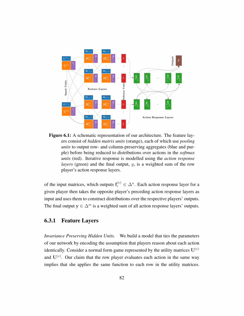
H(r)1,1

H1,1↓

H1,1 ↓

...

H(r)1,j

H1,j↓

H1,j ↓

H(r)2,1

H2,1↓

H2,1 ↓

...

H(r)2,j

H2,j↓

H2,j ↓

. . .

. . .

f1

...

fj

Feature Layers

Outp

ut

InputUnits

Softmax

Units

H(c)1,1

H1,1↓

H1,1 ↓

...

H(c)1,j

H1,j↓

H1,j ↓

H(c)2,1

H2,1↓

H2,1 ↓

...

H(c)2,j

H2,j↓

H2,j ↓

. . .

. . .

f1

...

fj

U(r)

U(r

)↓

U(r) ↓

U(c)

U(c

)↓

U(c) ↓ar(r)

0

ar(r)

1 ...ar(r)

k−1

ar(r)

k

ar(c)0

ar(c)1 ...

ar(c)k−

1

y

Action Response Layers

Figure 6.1: A schematic representation of our architecture. The feature lay-ers consist of hidden matrix units (orange), each of which use poolingunits to output row- and column-preserving aggregates (blue and pur-ple) before being reduced to distributions over actions in the softmaxunits (red). Iterative response is modelled using the action responselayers (green) and the final output, y, is a weighted sum of the rowplayer’s action response layers.

of the input matrices, which outputs f (c)i ∈ ∆n. Each action response layer for a

given player then takes the opposite player’s preceding action response layers asinput and uses them to construct distributions over the respective players’ outputs.The final output y ∈ ∆m is a weighted sum of all action response layers’ outputs.

6.3.1 Feature Layers

Invariance Preserving Hidden Units. We build a model that ties the parametersof our network by encoding the assumption that players reason about each actionidentically. Consider a normal form game represented by the utility matrices U(r)

and U(c). Our claim that the row player evaluates each action in the same wayimplies that she applies the same function to each row in the utility matrices.

82

Thus the weights associated with each row of U(r) and U(c) must be the same.Similarly, the corresponding assumption about the column player implies that theweights associated with each column of U(r) and U(c) must also be the same. Wecan satisfy both assumptions by applying a single scalar weight to each of theutility matrices, computing wrU(r) + wcU(c). This idea can be generalized as ina standard feed-forward network to allow us to fit more complex functions. Ahidden matrix unit taking all the preceding hidden matrix units as input can becalculated as

Hl,i = φ

∑j

wl,i,j Hl−1,j + bl,i

Hl,i ∈ Rm×n,

where Hl,i is the ith hidden unit matrix for layer l, wl,i,j is the jth scalar weight, bl,iis a scalar bias variable, and φ is a non-linear activation function applied element-wise. Notice that, as in a traditional feed-forward neural network, the output ofeach hidden unit is simply a nonlinear transformation of the weighted sum of thepreceding layer’s hidden units. Our architecture differs by maintaining a matrix ateach hidden unit instead of a scalar. So while in a traditional feed-forward networkeach hidden unit maps the previous layer’s vector of outputs into a scalar output,in our architecture each hidden unit maps a tensor of outputs from the previouslayer into a matrix output.

Tying weights in this way reduces the number of parameters in our networkby a factor of nm, offering two benefits. First, it reduces the degree to whichthe network is able to overfit; second and more importantly, it makes the modelinvariant to the size of the input matrices. To see this, notice that each hiddenunit maps from a tensor containing the k output matrices of the preceding layer inRk×m×n to a matrix in Rm×n using k weights. Thus our number of parameters ineach layer depends on the number of hidden units in the preceding layer, but noton the size of the input and output matrices. This allows the model to generalizeto input sizes that do not appear in training data.

83

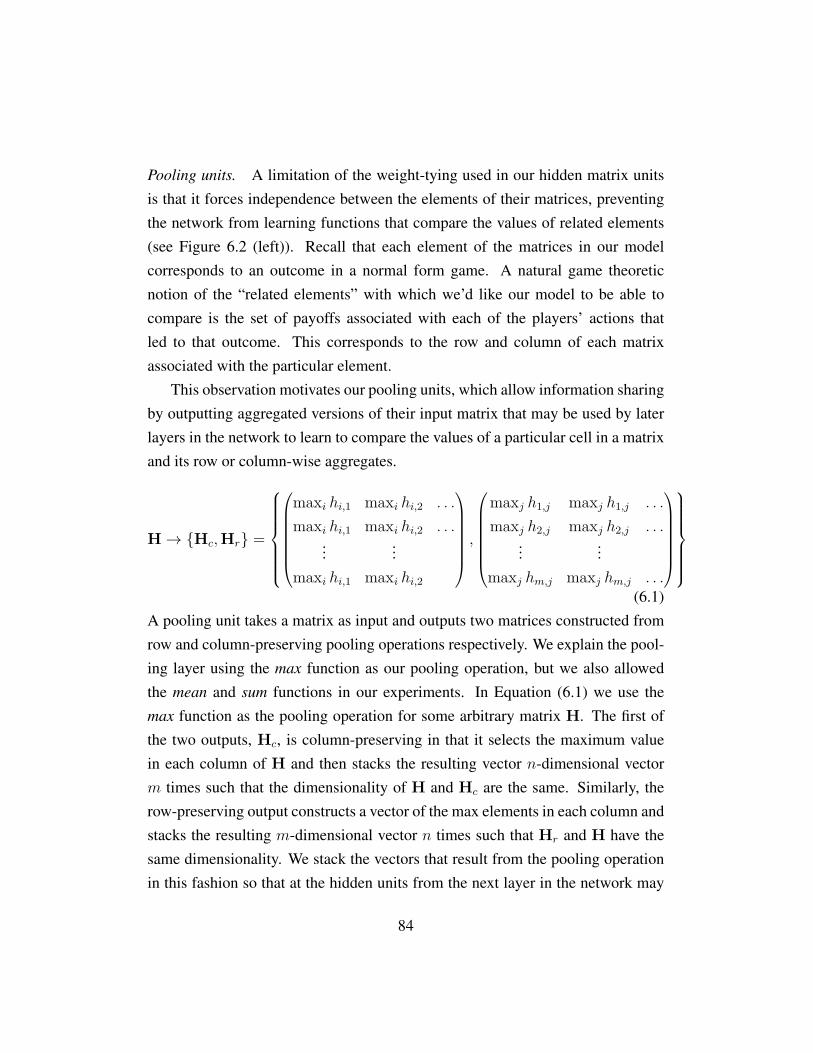
Pooling units. A limitation of the weight-tying used in our hidden matrix unitsis that it forces independence between the elements of their matrices, preventingthe network from learning functions that compare the values of related elements(see Figure 6.2 (left)). Recall that each element of the matrices in our modelcorresponds to an outcome in a normal form game. A natural game theoreticnotion of the “related elements” with which we’d like our model to be able tocompare is the set of payoffs associated with each of the players’ actions thatled to that outcome. This corresponds to the row and column of each matrixassociated with the particular element.

This observation motivates our pooling units, which allow information sharingby outputting aggregated versions of their input matrix that may be used by laterlayers in the network to learn to compare the values of a particular cell in a matrixand its row or column-wise aggregates.

H→ {Hc,Hr} =

maxi hi,1 maxi hi,2 . . .

maxi hi,1 maxi hi,2 . . ....

...maxi hi,1 maxi hi,2

,

maxj h1,j maxj h1,j . . .

maxj h2,j maxj h2,j . . ....

...maxj hm,j maxj hm,j . . .

(6.1)

A pooling unit takes a matrix as input and outputs two matrices constructed fromrow and column-preserving pooling operations respectively. We explain the pool-ing layer using the max function as our pooling operation, but we also allowedthe mean and sum functions in our experiments. In Equation (6.1) we use themax function as the pooling operation for some arbitrary matrix H. The first ofthe two outputs, Hc, is column-preserving in that it selects the maximum valuein each column of H and then stacks the resulting vector n-dimensional vectorm times such that the dimensionality of H and Hc are the same. Similarly, therow-preserving output constructs a vector of the max elements in each column andstacks the resulting m-dimensional vector n times such that Hr and H have thesame dimensionality. We stack the vectors that result from the pooling operationin this fashion so that at the hidden units from the next layer in the network may

84

Figure 3: Left: Without pooling units, each element of every hidden matrix unit depends only on thecorresponding elements in the units from the layer below; e.g., the middle element highlighted inred depends only on the value of the elements of the matrices highlighted in orange. Right: Withpooling units at each layer in the network, each element of every hidden matrix unit depends both onthe corresponding elements in the units below and the pooled quantity from each row and column.E.g., the light blue and purple blocks represent the row and column-wise aggregates corresponding totheir adjacent matrices. The dark blue and purple blocks show which of these values the red elementdepends on. Thus, the red element depends on both the dark- and light-shaded orange cells.JH: TODO: add level labels

Action Response Layers The feature layers described above are sufficient to meet our objective203

of mapping from the input payoff matrices to a distribution over the row player’s actions. However,204

this architecture is not capable of explicitly representing iterative strategic reasoning, which the205

behavioral game theory literature has identified as an important modeling ingredient. We incorporate206

this ingredient using action response layers: the first player can respond to the second’s beliefs,207

the second can respond to this response by the first player, and so on to some finite depth. The208

proportion of players in the population who iterate at each depth is a parameter of the model; thus,209

our architecture is also able to learn not to perform iterative reasoning.210

More formally, we begin by denoting the output of the feature layers as ar(r)0 =

Pki=1 w

(r)0i f

(r)i ,211

where we now include an index (r) to refer to the output of row player’s action response layer212

ar(r)0 2 �m. Similarly, by applying the feature layers to a transposed version of the input matrices,213

the model also outputs a corresponding ar(c)0 2 �n for the column player which expresses the row214

player’s beliefs about which actions the column player will choose. Each action response layer215

composes its output by calculating the expected value of an internal representation of utility with216

respect to its belief distribution over the opposition actions. For this internal representation of utility217

we chose simply a weighted sum of the final layer of the hidden layers,P

i wiHL,i, because each218

HL,i is already some non-linear transformation of the original payoff matrix, and so this allows the219

model to express utility as a transformation of the original payoffs. Given the matrix that results from220

this sum, we can compute expected utility with respect to the vector of beliefs about the opposition’s221

choice of actions, ar(c)j , by simply taking the dot product of the weighted sum and beliefs. When222

we iterate this process of responding to beliefs about one’s opposition more than once, higher level223

players will respond to beliefs, ari, for all i less their level and then output a weighted combination224

of these responses using some weights, vl,i. Putting this together, the lth action response layer for the225

row player (r) is defined as226

ar(r)l = softmax

�l

l�1X

j=0

v(r)l,j

kX

i=1

w(r)l,i H

(r)L,i

!· ar(c)

j

!!, ar

(r)l 2 �m, l 2 {1, ..., K},

where l indexes the action response layer, �l is a scalar sharpness parameter that allows us to sharpen227

the resulting distribution, w(r)l,i and v

(r)l,j are scalar weights, HL,i are the row player’s k hidden units228

from the final hidden layer L, ar(c)j is the output of the column player’s jth action response layer and229

K is the total number of action response layers. We constrain w(r)li and v

(r)lj to the simplex and use230

�l to sharpen the output distribution so that we can optimize the sharpness of the distribution and231

relative weighting of its terms independently. We build up the column player’s action response layer,232

ar(c)l , similarly, using the column player’s internal utility representation, H(c)

L,i, responding to the row233

player’s action response layers, ar(r)l . These layers are not used in the final output directly but are234

relied upon by subsequent action response layers of the row player.235

6

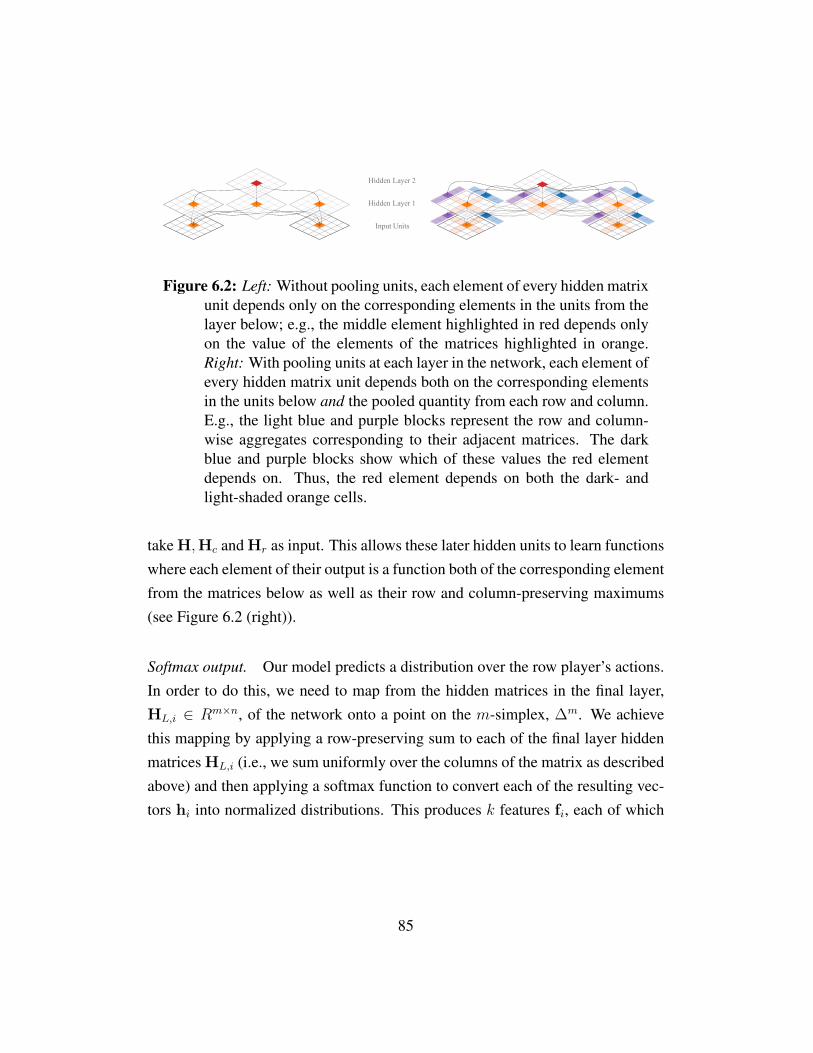
Figure 3: Left: Without pooling units, each element of every hidden matrix unit depends only on thecorresponding elements in the units from the layer below; e.g., the middle element highlighted inred depends only on the value of the elements of the matrices highlighted in orange. Right: Withpooling units at each layer in the network, each element of every hidden matrix unit depends both onthe corresponding elements in the units below and the pooled quantity from each row and column.E.g., the light blue and purple blocks represent the row and column-wise aggregates corresponding totheir adjacent matrices. The dark blue and purple blocks show which of these values the red elementdepends on. Thus, the red element depends on both the dark- and light-shaded orange cells.JH: TODO: add level labels

Action Response Layers The feature layers described above are sufficient to meet our objective203

of mapping from the input payoff matrices to a distribution over the row player’s actions. However,204

this architecture is not capable of explicitly representing iterative strategic reasoning, which the205

behavioral game theory literature has identified as an important modeling ingredient. We incorporate206

this ingredient using action response layers: the first player can respond to the second’s beliefs,207

the second can respond to this response by the first player, and so on to some finite depth. The208

proportion of players in the population who iterate at each depth is a parameter of the model; thus,209

our architecture is also able to learn not to perform iterative reasoning.210

More formally, we begin by denoting the output of the feature layers as ar(r)0 =

Pki=1 w

(r)0i f

(r)i ,211

where we now include an index (r) to refer to the output of row player’s action response layer212

ar(r)0 2 �m. Similarly, by applying the feature layers to a transposed version of the input matrices,213

the model also outputs a corresponding ar(c)0 2 �n for the column player which expresses the row214

player’s beliefs about which actions the column player will choose. Each action response layer215

composes its output by calculating the expected value of an internal representation of utility with216

respect to its belief distribution over the opposition actions. For this internal representation of utility217

we chose simply a weighted sum of the final layer of the hidden layers,P

i wiHL,i, because each218

HL,i is already some non-linear transformation of the original payoff matrix, and so this allows the219

model to express utility as a transformation of the original payoffs. Given the matrix that results from220

this sum, we can compute expected utility with respect to the vector of beliefs about the opposition’s221

choice of actions, ar(c)j , by simply taking the dot product of the weighted sum and beliefs. When222

we iterate this process of responding to beliefs about one’s opposition more than once, higher level223

players will respond to beliefs, ari, for all i less their level and then output a weighted combination224

of these responses using some weights, vl,i. Putting this together, the lth action response layer for the225

row player (r) is defined as226

ar(r)l = softmax

�l

l�1X

j=0

v(r)l,j

kX

i=1

w(r)l,i H

(r)L,i

!· ar(c)

j

!!, ar

(r)l 2 �m, l 2 {1, ..., K},

where l indexes the action response layer, �l is a scalar sharpness parameter that allows us to sharpen227

the resulting distribution, w(r)l,i and v

(r)l,j are scalar weights, HL,i are the row player’s k hidden units228

from the final hidden layer L, ar(c)j is the output of the column player’s jth action response layer and229

K is the total number of action response layers. We constrain w(r)li and v

(r)lj to the simplex and use230

�l to sharpen the output distribution so that we can optimize the sharpness of the distribution and231

relative weighting of its terms independently. We build up the column player’s action response layer,232

ar(c)l , similarly, using the column player’s internal utility representation, H(c)

L,i, responding to the row233

player’s action response layers, ar(r)l . These layers are not used in the final output directly but are234

relied upon by subsequent action response layers of the row player.235

6

Input Units

Hidden Layer 1

Hidden Layer 2

Figure 6.2: Left: Without pooling units, each element of every hidden matrixunit depends only on the corresponding elements in the units from thelayer below; e.g., the middle element highlighted in red depends onlyon the value of the elements of the matrices highlighted in orange.Right: With pooling units at each layer in the network, each element ofevery hidden matrix unit depends both on the corresponding elementsin the units below and the pooled quantity from each row and column.E.g., the light blue and purple blocks represent the row and column-wise aggregates corresponding to their adjacent matrices. The darkblue and purple blocks show which of these values the red elementdepends on. Thus, the red element depends on both the dark- andlight-shaded orange cells.

take H,Hc and Hr as input. This allows these later hidden units to learn functionswhere each element of their output is a function both of the corresponding elementfrom the matrices below as well as their row and column-preserving maximums(see Figure 6.2 (right)).

Softmax output. Our model predicts a distribution over the row player’s actions.In order to do this, we need to map from the hidden matrices in the final layer,HL,i ∈ Rm×n, of the network onto a point on the m-simplex, ∆m. We achievethis mapping by applying a row-preserving sum to each of the final layer hiddenmatrices HL,i (i.e., we sum uniformly over the columns of the matrix as describedabove) and then applying a softmax function to convert each of the resulting vec-tors hi into normalized distributions. This produces k features fi, each of which

85

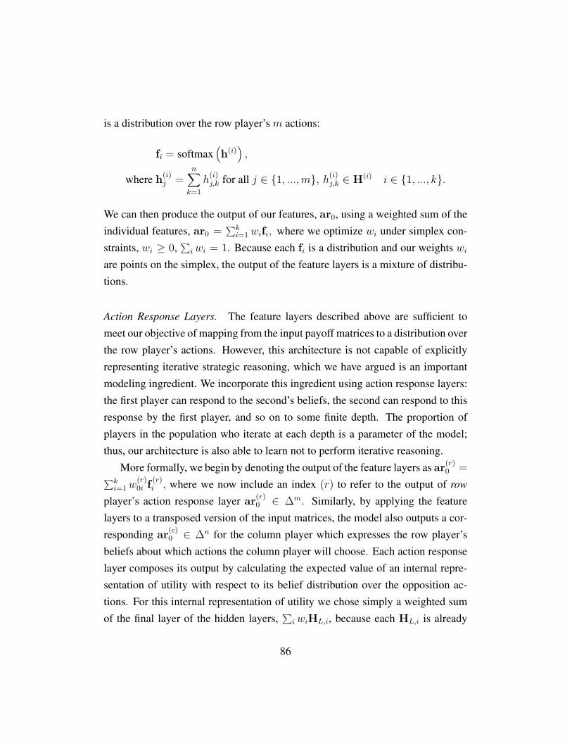
is a distribution over the row player’s m actions:

fi = softmax(h(i)

),

where h(i)j =

n∑k=1

h(i)j,k for all j ∈ {1, ...,m}, h(i)

j,k ∈ H(i) i ∈ {1, ..., k}.

We can then produce the output of our features, ar0, using a weighted sum of theindividual features, ar0 = ∑k

i=1 wifi, where we optimize wi under simplex con-straints, wi ≥ 0,

∑iwi = 1. Because each fi is a distribution and our weights wi

are points on the simplex, the output of the feature layers is a mixture of distribu-tions.

Action Response Layers. The feature layers described above are sufficient tomeet our objective of mapping from the input payoff matrices to a distribution overthe row player’s actions. However, this architecture is not capable of explicitlyrepresenting iterative strategic reasoning, which we have argued is an importantmodeling ingredient. We incorporate this ingredient using action response layers:the first player can respond to the second’s beliefs, the second can respond to thisresponse by the first player, and so on to some finite depth. The proportion ofplayers in the population who iterate at each depth is a parameter of the model;thus, our architecture is also able to learn not to perform iterative reasoning.

More formally, we begin by denoting the output of the feature layers as ar(r)0 =∑k

i=1 w(r)0i f (r)

i , where we now include an index (r) to refer to the output of row

player’s action response layer ar(r)0 ∈ ∆m. Similarly, by applying the feature

layers to a transposed version of the input matrices, the model also outputs a cor-responding ar(c)

0 ∈ ∆n for the column player which expresses the row player’sbeliefs about which actions the column player will choose. Each action responselayer composes its output by calculating the expected value of an internal repre-sentation of utility with respect to its belief distribution over the opposition ac-tions. For this internal representation of utility we chose simply a weighted sumof the final layer of the hidden layers,

∑iwiHL,i, because each HL,i is already

86

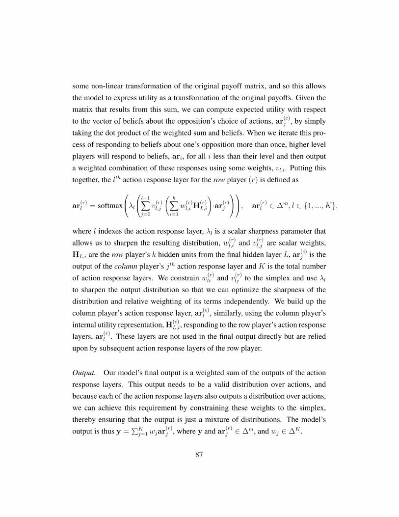
some non-linear transformation of the original payoff matrix, and so this allowsthe model to express utility as a transformation of the original payoffs. Given thematrix that results from this sum, we can compute expected utility with respectto the vector of beliefs about the opposition’s choice of actions, ar(c)

j , by simplytaking the dot product of the weighted sum and beliefs. When we iterate this pro-cess of responding to beliefs about one’s opposition more than once, higher levelplayers will respond to beliefs, ari, for all i less than their level and then outputa weighted combination of these responses using some weights, vl,i. Putting thistogether, the lth action response layer for the row player (r) is defined as

ar(r)l = softmax

λll−1∑j=0

v(r)l,j

(k∑i=1

w(r)l,i H(r)

L,i

)·ar(c)

j

, ar(r)l ∈ ∆m, l ∈ {1, ..., K},

where l indexes the action response layer, λl is a scalar sharpness parameter thatallows us to sharpen the resulting distribution, w(r)

l,i and v(r)l,j are scalar weights,

HL,i are the row player’s k hidden units from the final hidden layer L, ar(c)j is the

output of the column player’s jth action response layer and K is the total numberof action response layers. We constrain w(r)

li and v(r)lj to the simplex and use λl

to sharpen the output distribution so that we can optimize the sharpness of thedistribution and relative weighting of its terms independently. We build up thecolumn player’s action response layer, ar(c)

l , similarly, using the column player’sinternal utility representation, H(c)

L,i, responding to the row player’s action responselayers, ar(r)

l . These layers are not used in the final output directly but are reliedupon by subsequent action response layers of the row player.

Output. Our model’s final output is a weighted sum of the outputs of the actionresponse layers. This output needs to be a valid distribution over actions, andbecause each of the action response layers also outputs a distribution over actions,we can achieve this requirement by constraining these weights to the simplex,thereby ensuring that the output is just a mixture of distributions. The model’soutput is thus y = ∑K

j=1 wjar(r)j , where y and ar(r)

j ∈ ∆m, and wj ∈ ∆K .

87

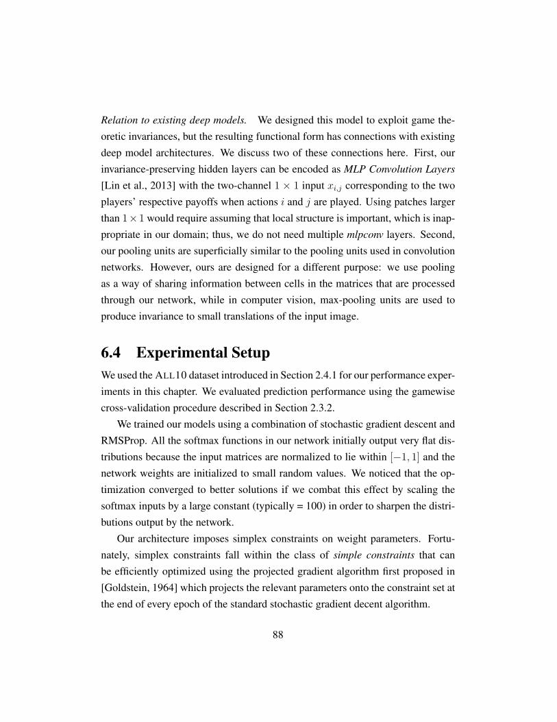
Relation to existing deep models. We designed this model to exploit game the-oretic invariances, but the resulting functional form has connections with existingdeep model architectures. We discuss two of these connections here. First, ourinvariance-preserving hidden layers can be encoded as MLP Convolution Layers

[Lin et al., 2013] with the two-channel 1 × 1 input xi,j corresponding to the twoplayers’ respective payoffs when actions i and j are played. Using patches largerthan 1×1 would require assuming that local structure is important, which is inap-propriate in our domain; thus, we do not need multiple mlpconv layers. Second,our pooling units are superficially similar to the pooling units used in convolutionnetworks. However, ours are designed for a different purpose: we use poolingas a way of sharing information between cells in the matrices that are processedthrough our network, while in computer vision, max-pooling units are used toproduce invariance to small translations of the input image.

6.4 Experimental SetupWe used the ALL10 dataset introduced in Section 2.4.1 for our performance exper-iments in this chapter. We evaluated prediction performance using the gamewisecross-validation procedure described in Section 2.3.2.

We trained our models using a combination of stochastic gradient descent andRMSProp. All the softmax functions in our network initially output very flat dis-tributions because the input matrices are normalized to lie within [−1, 1] and thenetwork weights are initialized to small random values. We noticed that the op-timization converged to better solutions if we combat this effect by scaling thesoftmax inputs by a large constant (typically = 100) in order to sharpen the distri-butions output by the network.

Our architecture imposes simplex constraints on weight parameters. Fortu-nately, simplex constraints fall within the class of simple constraints that canbe efficiently optimized using the projected gradient algorithm first proposed in[Goldstein, 1964] which projects the relevant parameters onto the constraint set atthe end of every epoch of the standard stochastic gradient decent algorithm.

88

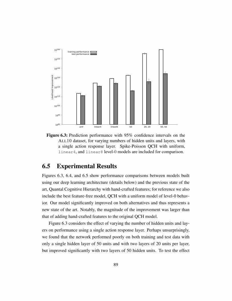
1080

1090

10100

10110

10120

10130

10140

10150

10160

unif linear4 linear8 50 20, 20 50, 50

Like

lihood

im

pro

vem

ent

training performancetest performance

Figure 6.3: Prediction performance with 95% confidence intervals on theALL10 dataset, for varying numbers of hidden units and layers, witha single action response layer. Spike-Poisson QCH with uniform,linear4, and linear8 level-0 models are included for comparison.

6.5 Experimental ResultsFigures 6.3, 6.4, and 6.5 show performance comparisons between models builtusing our deep learning architecture (details below) and the previous state of theart, Quantal Cognitive Hierarchy with hand-crafted features; for reference we alsoinclude the best feature-free model, QCH with a uniform model of level-0 behav-ior. Our model significantly improved on both alternatives and thus represents anew state of the art. Notably, the magnitude of the improvement was larger thanthat of adding hand-crafted features to the original QCH model.

Figure 6.3 considers the effect of varying the number of hidden units and lay-ers on performance using a single action response layer. Perhaps unsurprisingly,we found that the network performed poorly on both training and test data withonly a single hidden layer of 50 units and with two layers of 20 units per layer,but improved significantly with two layers of 50 hidden units. To test the effect

89

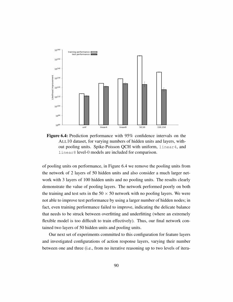
1080

1090

10100

10110

10120

10130

10140

10150

10160

unif linear4 linear8 50,50 150,150

Like

lihood

im

pro

vem

ent

training performancetest performance

Figure 6.4: Prediction performance with 95% confidence intervals on theALL10 dataset, for varying numbers of hidden units and layers, with-out pooling units. Spike-Poisson QCH with uniform, linear4, andlinear8 level-0 models are included for comparison.

of pooling units on performance, in Figure 6.4 we remove the pooling units fromthe network of 2 layers of 50 hidden units and also consider a much larger net-work with 3 layers of 100 hidden units and no pooling units. The results clearlydemonstrate the value of pooling layers. The network performed poorly on boththe training and test sets in the 50 × 50 network with no pooling layers. We werenot able to improve test performance by using a larger number of hidden nodes; infact, even training performance failed to improve, indicating the delicate balancethat needs to be struck between overfitting and underfitting (where an extremelyflexible model is too difficult to train effectively). Thus, our final network con-tained two layers of 50 hidden units and pooling units.

Our next set of experiments committed to this configuration for feature layersand investigated configurations of action response layers, varying their numberbetween one and three (i.e., from no iterative reasoning up to two levels of itera-

90

1080

1090

10100

10110

10120

10130

10140

10150

10160

unif linear4 linear8 1 2 3

Like

lihood

im

pro

vem

ent

training performancetest performance

Figure 6.5: Prediction performance with 95% confidence intervals on theALL10 dataset, for GameNet architecture with two layers of 50 hid-den units, with pooling units, with varying numbers of action responselayers. Spike-Poisson QCH with uniform, linear4, and linear8

level-0 models are included for comparison.

tive reasoning; see Figure 6.5). All networks with more than one action responselayer showed clear signs of overfitting: performance on the training set improvedsignificantly but test set performance suffered. Thus, our final network used onlyone action response layer. We nevertheless remain committed to an architecturethat can capture iterative strategic reasoning; we intend to investigate more ef-fective methods of regularizing the parameters of action response layers in futurework.

6.6 Regular Neural Network PerformanceFigure 6.6 compares the performance of our architecture with that of a regularfeed forward neural network, with and without data augmentation and the previousstate-of-the-art model on this dataset. Since a regular feed-forward network can

91

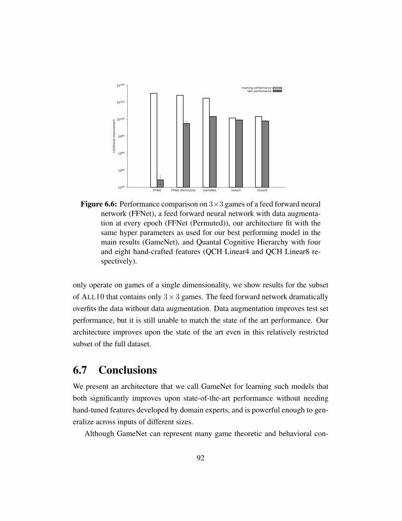
1020

1040

1060

1080

10100

10120

10140

FFNet FFNet (Permuted) GameNet linear4 linear8

Like

lihood im

pro

vem

ent

training performancetest performance

Figure 6.6: Performance comparison on 3×3 games of a feed forward neuralnetwork (FFNet), a feed forward neural network with data augmenta-tion at every epoch (FFNet (Permuted)), our architecture fit with thesame hyper parameters as used for our best performing model in themain results (GameNet), and Quantal Cognitive Hierarchy with fourand eight hand-crafted features (QCH Linear4 and QCH Linear8 re-spectively).

only operate on games of a single dimensionality, we show results for the subsetof ALL10 that contains only 3×3 games. The feed forward network dramaticallyoverfits the data without data augmentation. Data augmentation improves test setperformance, but it is still unable to match the state of the art performance. Ourarchitecture improves upon the state of the art even in this relatively restrictedsubset of the full dataset.

6.7 ConclusionsWe present an architecture that we call GameNet for learning such models thatboth significantly improves upon state-of-the-art performance without needinghand-tuned features developed by domain experts, and is powerful enough to gen-eralize across inputs of different sizes.

Although GameNet can represent many game theoretic and behavioral con-

92

cepts, it is not perfectly expressive. We plan to explore the effect of including ad-ditional operators that are able to encode game theoretic concepts that we believeour model cannot currently represent, such as dominance and framing effects.

Overall, we believe that deep learning is an extremely promising direction forconstructing models of human strategic behavior. Our architecture demonstratesthat it is possible to learn a highly performant behavioral model automaticallyfrom data, with minimal need for fine-tuning by domain experts.

Although GameNet outperforms the structural models of earlier chapters, itprovides no insight into how or why people choose certain actions. The deepmodel’s superior prediction performance demonstrates that there is room to im-prove the structural models. Ideally, we would like to combine the interpretabilityof a structural model with the superior prediction performance of a deep model.

93

Part II

Application Domain: Peer Grading

94

Chapter 7

Incentivizing Evaluation via LimitedAccess to Ground Truth

In this part, we shift our attention from modeling human behavior in generic strate-gic environments to the specific strategic setting of peer grading. We begin bytheoretically analyzing the incentivized elicitation setting, which includes peergrading as a special case. In the next chapter, we will present a case study of areal-life peer grading system.

This chapter does not directly build upon the behavioral foundation of Part I.Instead, we analyze the properties of the Nash equilibria of elicitation mecha-nisms. We took this approach for two reasons. First, this chapter’s results canbe understood as showing that peer-prediction mechanisms do not succeed evenby their own standards; without any relaxation of rationality assumptions, an onlyslightly more realistic setting is enough to invalidate their equilibrium guarantees.Second, we show that the mechanism that most efficiently uses ground truth pro-duces a dominant strategy for the agents. Many of the strategic considerations ofPart I’s framework (reasoning about nonstrategic agents, limits to strategic rea-soning) do not apply in the context of a dominant-strategy mechanism, where anagent need not reason strategically about the other agents at all.1

1Other behavioral considerations, such as quantal response, do still apply in such a setting, but

95

7.1 IntroductionThere are many practical settings in which it is important to collect accurate eval-uations about objects of interest from dispersed individuals. For example, manymillions of users rely on feedback from Rotten Tomatoes, Yelp, and TripAdvisorto choose among competing movies, restaurants, and travel destinations. Crowd-sourcing platforms provide another example, enabling the collection of semanticlabels of images and online content for use in training machine learning algo-rithms.

We are particularly motivated by the peer grading problem, which we willuse as a running example. Students benefit from open-ended assignments such asessays or proofs. However, such assignments are used relatively sparingly, partic-ularly in large classes, because they require considerable time and effort to gradeproperly. An efficient and scalable alternative is having students grade each other(and, in the process, learn from each other’s work). Many peer grading systemshave been proposed and evaluated in the education literature [Hamer et al., 2005;Cho and Schunn, 2007a; Pare and Joordens, 2008; de Alfaro and Shavlovsky,2014a; Kulkarni et al., 2014; and Chapter 8 of this dissertation], albeit with a fo-cus on evaluating the accuracy of grades collected under the assumption of fullcooperation by students.

However, no experienced teacher would expect all students to behave non-strategically when asked to invest effort in a time-consuming task. An effectivepeer grading system must therefore provide motivation for students to formulateevaluations carefully and to report them honestly. Many approaches have beendeveloped to provide such motivation. One notable category is peer-predictionmethods [Prelec, 2004; Miller et al., 2005; Jurca and Faltings, 2009; Faltings et al.,2012; Witkowski and Parkes, 2012; Witkowski et al., 2013; Dasgupta and Ghosh,2013; Witkowski and Parkes, 2013; Radanovic and Faltings, 2013, 2014; Riley,2014; Zhang and Chen, 2014; Waggoner and Chen, 2014; Kamble et al., 2015;Kong et al., 2016; Shnayder et al., 2016]. In order to motivate each agent to re-

we do not explore them in this chapter.

96

veal his private, informative signal, peer-prediction methods offer a reward basedon how each agent’s reports compare with those of his peers. Such rewards aredesigned to induce truth telling in equilibrium—that is, they create a situation inwhich each agent has an interest in investing effort and revealing his private andinformative signal truthfully, as long as he believes that all other agents will dothe same.

Even if they do offer a truthful equilibrium, peer-prediction methods also al-ways induce other uninformative equilibria, the existence of which is inevitable[Jurca and Faltings, 2009; Waggoner and Chen, 2014]. Intuitively, if no otheragent follows a strategy that depends on her private information, there is no rea-son for a given agent to deviate in a way that does so either: agents can only berewarded for coordination, not for accuracy. When private information is costlyto obtain, uninformative equilibria are typically less demanding for agents to play.This raises significant doubt about whether peer-prediction methods can moti-vate truthful reporting in practice. Experimental evaluations of peer-predictionmethods have mixed results. Some studies showed that agents reported truthfully[Shaw et al., 2011; John et al., 2012; Faltings et al., 2014]; another study foundthat agents colluded on uninformative equilibria [Gao et al., 2014].

Recent progress on peer-prediction mechanisms has focused on making thetruthful equilibrium Pareto dominant, i.e., (weakly) more rewarding to every agentthan any other equilibrium [Dasgupta and Ghosh, 2013; Witkowski and Parkes,2013; Kamble et al., 2015; Radanovic and Faltings, 2015; Shnayder et al., 2016].This can be achieved by rewarding agents based on the distributions of their re-ports for multiple objects. However, we show in this chapter that such argumentsrely critically on the assumption that every agent has access to only one privatesignal per object. This is often untrue in practice; e.g., in peer grading, by taking aquick glance at an essay a student can observe characteristics such as length, for-matting and the prevalence of grammatical errors. These characteristics requirehardly any effort to observe, can be arbitrarily uninformative about true quality,and are of no interest to the mechanism. Yet their existence provides a means for

97

the agents to coordinate. We build on this intuition to prove that no mechanismcan guarantee that an equilibrium in which all agents truthfully report their in-formative signals is always Pareto dominant. Furthermore, we show that for anymechanism, the truthful equilibrium is always Pareto dominated in some settings.

Motivated by these negative results, we move on to consider a setting in whichthe operator of the mechanism has access to trusted evaluators (e.g., teaching as-sistants) who can reliably provide noisy but informative signals of the object’strue quality. This allows for a hybrid mechanism that blends peer-prediction withcomparison to trusted reports. With a fixed probability, the mechanism obtains atrusted report and rewards the agent based on the agreement between the agent’sreport and the trusted report [Jurca and Faltings, 2005]. Otherwise, the mechanismrewards the agent using a peer-prediction mechanism. Such hybrid mechanismscan yield stronger incentive guarantees than other peer-prediction mechanisms,such as achieving truthful reporting of informative signals in Pareto-dominantequilibrium [e.g., Jurca and Faltings, 2005; Dasgupta and Ghosh, 2013]. Intu-itively, if an agent seeks to be consistently close to a trusted report, then his beststrategy is to reveal his informative signal truthfully.

In fact, the availability of trusted reports is so powerful that it gives us theoption of dispensing with peer-prediction altogether. Specifically, we can rewardstudents based on agreement with the trusted report when the latter is available,but simply pay students a constant reward otherwise. Indeed, in Chapter 8 we de-scribe such a peer grading system and show that it worked effectively in practice,based on a study across three years of a large class. This mechanism has evenstronger incentive properties than the hybrid mechanism—because it induces asingle-agent game, it can give rise to dominant-strategy truthfulness.

This chapter’s main focus is on comparing these two approaches in terms ofthe number of trusted reports that they require. One might expect that the peer-prediction approach would have the edge, both because it relies on a weaker solu-tion concept and because it leverages a second source of information reported byother agents. Surprisingly, we prove that this intuition is backwards. We identify a

98

simple sufficient condition, which, if satisfied, guarantees that the peer-insensitivemechanism offers the dominant strategy of truthful reporting of informative sig-nals while querying trusted reports with a lower probability than is required fora peer-prediction mechanism to motivate truthful reporting in Pareto-dominantequilibrium. We then show that all applicable peer-prediction mechanisms ofwhich we are aware satisfy this sufficient condition.

7.2 Peer-Prediction MechanismsWe begin by formally defining the game theoretic setting in which we will studythe elicitation problem. A mechanism designer wishes to elicit information abouta set O of objects from n risk-neutral agents. Each object j has a latent qualityqj ∈ Q, where Q is a finite set. For each object j, agent i has access to twopieces of private information:2 a high-quality signal shij ∈ Q, which is drawnfrom a distribution conditional on the actual quality qj; and a low-quality signal

slj , which may be uncorrelated with qj . The joint distributions of both the high-quality and low-quality signals are common knowledge among the agents. Inparticular, an agent i can form a belief about the high-quality signal of anotheragent i′ by conditioning on his own high-quality signal.

We assume that agents can observe the low-quality signal slj without effort,but that observing the high-quality signal shij requires a constant effort cE > 0.Agents may strategize over both whether to incur the cost of effort to observe thehigh-quality signal and over what to report. The mechanism designer’s goal isto incentivize each agent to both observe the high-quality signal, and to truthfullyreport it. We say that a mechanism has a truthful equilibrium when it is an equilib-rium for agents to observe the high-quality signal and truthfully report it (and, forsome mechanisms, their posterior belief about other agents’ high-quality signals).

2We depart from a standard assumption in the literature: that agents receive only a single signalabout any object. We argue that agents also inevitably have access to simple metadata about anyobject they are asked to evaluate, such as its name, location, color, the length of its description,etc. We model all of this metadata as a second, costless signal that is perfectly correlated acrossagents.

99

In the context of peer grading, the agents are the students assigned to gradeeach others’ assignments, and the objects are the assignments. The high-qualitysignal is obtained by carefully reading and grading an assignment. The low-quality signal is obtained by observing trivial characteristics of the assignmentsuch as its length, title, formatting, etc.

The mechanism designer’s aim is to incentivize each agent i ∈ {1, . . . , n} togather and truthfully report information about every object j ∈ Ji ⊆ O; in thischapter we denote by Ji the set of objects assigned to an agent for evaluation,rather than the number of actions in a game as in Chapter 2. Let rij and bij

denote agent i’s signal and belief reports for object j respectively. A mechanismis defined by a reward function, which maps a profile of agent reports to a rewardfor each agent. We say that a mechanism is universal if it can be applied withoutprior knowledge of the distribution from which signals are elicited, and for anynumber of agents greater than or equal to 3.

Definition 12 (Universal peer-prediction mechanism). A peer-prediction mecha-nism is universal if it can be operated without knowledge of the joint distributionof the high-quality signals shij (i.e., it is “detail free” [Wilson, 1987]) and welldefined for any number of agents n ≥ 3.

We focus on universal mechanisms for two reasons. First, in practice, it is ex-tremely unrealistic to assume that a mechanism designer will have detailed knowl-edge of the joint signal distribution, so this allows us to focus on mechanisms thatare more likely to be used in practice. Second, it is relatively unrestrictive, asnearly all of the peer-prediction mechanisms in the literature satisfy universality.

Existing, universal peer-prediction mechanisms can be divided into three cate-gories: output agreement mechanisms, multi-object mechanisms, and belief basedmechanisms.

Output Agreement Mechanisms. Output agreement mechanisms only collect sig-nal reports from agents and reward an agent i for evaluating object j based onagents’ signal reports for the object [Faltings et al., 2012; Witkowski et al., 2013;

100

Waggoner and Chen, 2014]. Waggoner and Chen [2014] and Witkowski et al.[2013] studied the standard output agreement mechanism, where agent i is onlyrewarded when his signal report matches that of another randomly chosen agentj. Agent i’s reward is zi(r) = 1rij=ri′j

. The Faltings et al. [2012] mechanismalso rewards agents for agreement, scaled by the empirical frequency of the reportagreed upon. Agent i’s reward is zi(r) = α + β

1rij =ri′jF (ri′j) , where α > 0 and β > 0

are constants and F (rj) is the empirical frequency of rj .

Multi-Object Mechanisms. Multi-object mechanisms reward each agent basedon his reports for multiple objects [Dasgupta and Ghosh, 2013; Radanovic andFaltings, 2015; Kamble et al., 2015; Shnayder et al., 2016]. (The Shnayder et al.[2016] mechanism generalizes the Dasgupta and Ghosh [2013] mechanism to themulti-signal setting. Thus, we only refer to the Shnayder et al. [2016] mechanismbelow.)

The Shnayder et al. [2016] and Kamble et al. [2015] mechanisms also rewardagents for agreement, as in output agreement mechanisms. They extend outputagreement mechanisms by adding additional scaling terms to the reward. Thesescaling terms are intended to exploit correlations between multiple tasks to makethe truthful equilibrium dominate (a particular kind of) uninformative equilibria,by reducing the reward to agents who agree to an amount that is “unsurprising”given their reports on other objects.

The Shnayder et al. [2016] mechanism adds an additive scaling term to thereward for agreement. To compute the scaling term, consider two sets of non-overlapping tasks Si and Si′ such that agent i has evaluated all objects in Si butnone in Si′ and agent i′ has evaluated all objects in Si′ but none in Si. Let Fi(s)and Fi′(s) denote the frequency of signal s ∈ Q in sets Si and Si′ respectively.Agent i is rewarded according to zi(r) = 1rij=ri′j

−∑s∈Q Fi(s)Fi′(s).In contrast, the Kamble et al. [2015] mechanism adds a multiplicative scaling

term to the reward for agreement. To compute the scaling term, choose 2 agentsk and k′ uniformly at random. For each signal s ∈ Q, let f j(s) = 1rkj=s1rk′j=s.

101

Define f(s) =√

1N

∑j∈O f j(s). If f(s) ∈ {0, 1}, then agent i’s reward is 0.

Otherwise, agent i’s reward is 1rij=ri′j· Kf(s) for some constant K > 0.

The Radanovic and Faltings [2015] mechanism rewards the agents for reportagreement using a reward function inspired by the quadratic scoring rule. Toreward agent i for evaluating object j, first choose another random agent i′ whoalso evaluated object j. Then construct a sample Σi of reports which containsone report for every object that is not evaluated by agent i. The sample Σi isdouble-mixed if it contains all possible signal realizations at least twice. If Σi isnot double-mixed, agent i’s reward is 0. Otherwise, if Σi is double-mixed, themechanism chooses two objects j′ and j′′ (j′ 6= j, j′′ 6= j and j′ 6= j′′) suchthat the reports of j′ and j′′ in the sample are the same as agent i’s report for j,i.e. Σi(j′) = Σi(j′′) = rij . For each of j′ and j′′, randomly select two reportsri′′j′ and ri′′′j′′ . Agent i’s is rewarded according to zi(r) = 1

2 + 1ri′′j′=ri′j−

12∑s∈Q 1ri′′j′=s1ri′′′j′′=s.

Belief Based Mechanisms. Finally, some peer-prediction mechanisms collectboth signals and belief reports from agents and reward each agent based on allagents’ signal and belief reports for each object [Witkowski and Parkes, 2012,2013; Radanovic and Faltings, 2013, 2014; Riley, 2014]. Below, let R denote aproper scoring rule.

The robust Bayesian Truth Serum (BTS) [Witkowski and Parkes, 2012, 2013]rewards agent i for how well his belief report bi and shadowed belief report b′ipredict the signal reports of another randomly chosen agent k. Agent i’s rewardis zi(r, b) = R(b′i, rk) + R(bi, rk). Agent i’s shadowed belief report is calculatedbased on his signal report and another random agent j’s belief report: b′i = bj + δ

if ri = 1 and b′i = bj − δ if ri = 0 where δ = min(bj, 1− bj).The multi-valued robust BTS [Radanovic and Faltings, 2013] rewards agent

i if his signal report matches that of another random agent j and his belief re-port accurately predicts agent j’s signal report. Agent i’s reward is zi(r, b) =

1bj(ri)1ri=rj

+R(bi, rj).

102

The divergence-based BTS [Radanovic and Faltings, 2014] rewards agent iif his belief report accurately predicts another random agent j’s signal report.In addition, it penalizes agent i if his signal report matches that of agent j buthis belief report is sufficiently different from that of agent j. Agent i’s rewardis −1ri=rj ||D(bi,bj)>θ + R(bi, rj) where D(||) is the divergence associated to thestrictly proper scoring rule R, and θ is a parameter of the mechanism.

The Riley [2014] mechanism rewards agent i for how well his belief reportpredicts other agents’ signal reports. Moreover, agent i’s reward is bounded aboveby the score for the average belief report of other agents reporting the same signal.Formally, let δi = mins∈Q |{rj = s|j 6= i}| be the minimum number of otheragents who have reported any given signal. If δi = 0, agent i’s reward isR(bi, r−i).Otherwise, if δi ≥ 1, compute the proxy prediction qi(ri) to be the average beliefreport for all other agents who made the same signal report as agent i. Agent i’sreward is min{R(bi, r−i), R(qi(ri), r−i)}.

Non-Universal Mechanisms. We are aware of several additional peer-predictionmechanisms that we do not consider further in this chapter because they are notuniversal in the sense of Definition 12. The Miller et al. [2005]; Zhang and Chen[2014] and Kong et al. [2016] mechanisms all derive the agents’ posterior beliefsbased on their signal reports (hence requiring knowledge of the distribution fromwhich signals are drawn); they all then reward the agents based on how well thederived posterior belief predicts other agents’ signal reports using proper scoringrules. The Jurca and Faltings [2009] mechanism requires knowledge of the priordistribution over signals to construct rewards that either penalize or eliminatesymmetric, uninformative equilibria. The Bayesian Truth Serum (BTS) mecha-nism [Prelec, 2004] requires an infinite number of agents to guarantee the exis-tence of the truthful equilibrium. While we do not consider this mechanism, wenote that Prelec [2004] pioneered the idea of eliciting both signal and belief re-ports from each agent. This key idea was leveraged in much subsequent work tosustain the truthful equilibrium while not requiring the knowledge of the prior dis-

103

tributions of the signals to operate the mechanism [Witkowski and Parkes, 2012,2013; Radanovic and Faltings, 2013, 2014; Riley, 2014].

7.3 Impossibility of Pareto-Dominant, TruthfulElicitation

In this section, we show that when agents have access to multiple signals about anobject, Pareto-dominant truthful elicitation is impossible for any universal elicita-tion mechanism that computes agent rewards solely based on a profile of strategicagent reports (i.e., without any access to ground truth). The intuition is that with-out knowledge of the distributions from which the signals are drawn, the mech-anism cannot distinguish the signal that it hopes to elicit from other, irrelevantsignals. Thus, it cannot guarantee that the truthful equilibrium always yields thehighest rewards to all agents.

We focus on universal elicitation mechanisms that compute agent rewardssolely based on a profile of agent reports. Let M denote such a mechanism. Let asignal structure be a collection of signals {si}ni=1 drawn from a joint distributionF , where each agent i observes si. We say that a signal structure is M -elicitable

if there exists an equilibrium of M where every agent i truthfully reports si. LetπFi be agent i’s ex-ante expected reward in this equilibrium. A multi-signal en-

vironment is an environment in which the agents have access to at least two M -elicitable signal structures. We refer to the signal structure that the mechanismseeks to elicit as the high-quality signal, and all the others as low-quality signals.

Theorem 1. For any universal elicitation mechanism, there exists a multi-signal

environment in which the truthful equilibrium is not Pareto dominant.

Proof. Let F, F ′ be M -elicitable signal structures such that πFi ≥ πF′

i for all i,with πFi > πF

′i for some i. If no such pair of signal structures exists, then the

result follows directly, since the truthful equilibrium does not Pareto dominate anequilibrium where agents report a low-quality signal. Otherwise, consider a multi-signal environment where the high-quality signal is distributed according to F ′,

104

and a low-quality signal is distributed according to F . The equilibrium in whichagents reveal this low-quality signal Pareto dominates the truthful equilibrium inthis environment.

Now suppose that observing the high-quality signal is more costly to the agentsthan observing a low-quality signal. Concretely, assume that observing the high-quality signal has an additive cost of ci > 0 for each agent i, and observing alow-quality signal has zero cost. Call this a costly-observation multi-signal envi-

ronment. In this realistic environment, an even stronger result holds.

Theorem 2. For any universal elicitation mechanism, there exists a costly-observation

multi-signal environment in which the truthful equilibrium either does not exist or

is Pareto dominated.

Proof. Let F, F ′ be M -elicitable signal structures such that πFi ≥ πF′

i for all i.At least one such pair must exist, since every distribution has this relationship toitself. Fix a costly-observation multi-signal environment where the high-qualitysignal structure is jointly distributed according to F ′, and a low-quality signalstructure is jointly distributed according to F . If the mechanism has no truthfulequilibrium in this environment, then we are done. Otherwise, each agent’s ex-pected utility in the truthful equilibrium is πF ′i − ci < πFi . Hence every agentprefers the equilibrium in which agents reveal this low-quality signal, and thetruthful equilibrium is Pareto dominated.

The essential insight of these results is that, in the presence of multiple elic-itable signals, there is no way for a universal elicitation mechanism to be surewhich signal it is eliciting. In particular, the truthful equilibrium is only Paretodominant if the high-quality signal happens to be drawn from a distribution yield-ing higher reward than every other signal available to the agents. In costly-observation environments, the element of luck is even stronger. The truthful equi-librium is Pareto dominant only if the high-quality signal structure happens toyield sufficiently high reward to compensate for the cost of observing the signals.

105

One way for the mechanism designer to ensure that agents report the high-quality signal is to stochastically compare agents’ reports to reports known to becorrelated with that signal. In the next section, we introduce a class of mechanismsthat takes this approach.

7.4 Combining Elicitation with Limited Access toGround Truth

Elicitation mechanisms are designed for situations where it is infeasible for themechanism designer to evaluate each object herself. However, in practice, it isvirtually always possible, albeit costly, to obtain trusted reports, i.e. unbiasedevaluations of a subset of the objects. In the peer grading setting, the instructor andteaching assistants can always mark some of the assignments. Similarly, reviewsites could in principle hire an expert to evaluate restaurants or hotels that its usershave reviewed; and so on.

In this section, we define a class of mechanisms that take advantage of thislimited access to ground truth to circumvent the result from Section 7.3.

Definition 13 (spot-checking mechanism). A spot-checking mechanism is a tupleM = (p, y, z), where p is the spot check probability; y is a vector of functionsyij(rij, stj) called the spot check mechanism; and z is a vector of functions zij(b, r)called the unchecked mechanism.

Let ∆(Q) be the set of all distributions over the elements of Q. Each agenti makes a signal report rij ∈ Q, and a belief report bij ∈ ∆(Q) for each objectj ∈ Ji. The signal report is the signal that i claims to have observed, and the beliefreport represents i’s posterior belief over the signal reports of the other agents.

Agents may strategically choose whether or not to incur the cost of observingthe high-quality signal, and having chosen which signal to observe, may reportany function of either signal. Formally, let Gh

i = {g : Q → Q} be the set ofall full-effort pure strategies, where an agent observes the high-quality signal—incurring observation cost cE—and then reports a function g(shij) of the observed

106

value. Let Dl be the domain of slij . Let Gli = {g : Dl → Q} be the set of all no-

effort pure strategies, where an agent observes the low-quality signal—incurringno observation cost—and then reports a function gl(slij) of the observed value.The set of pure strategies available to an agent is thus Gh

i ∪ Gli. We assume that

agents apply the same strategy to every object that they evaluate; however, weallow agents to play a mixed strategy by choosing the mapping stochastically.

With probability p, the mechanism will spot check an agent i’s report for agiven object j. In this case, the mechanism obtains a trusted report—that is,a sample from the signal stj . The agent is then rewarded according to the spotcheck mechanism, applied to the profile of signal reports and spot checked objects.With probability 1 − p, the object is not spot checked, and the agent is rewardedaccording to the unchecked mechanism.

Thus, given a profile of signal reports r ∈ ∏i∈N Q

Ji and belief reports b ∈∏i∈N ∆(Q)Ji , an agent i receives a reward of πi = ∑

j∈Jiπij , where

πij =

yij(ri, st) if agent i’s report on object j is spot checked,

zij(b, r) otherwise.(7.1)

We assume that the mechanism designer has no value for the reward given tothe agents. Instead, we seek only to minimize the probability of spot-checkingrequired to make the truthful equilibrium either unique or Pareto dominant, sinceaccess to trusted reports is assumed to be costly.3 This models situations whereagents are rewarded by grades (as in peer grading), virtual points or badges (as inonline reviews), or other artificial currencies. In this work we compare two ap-proaches to using limited access to ground truth for elicitation. The first approachis to augment existing peer-prediction mechanisms with spot-checking:

Definition 14 (spot-checking peer-prediction mechanism). Let z be a peer-predictionmechanism. Then any spot-checking mechanism that uses z as its unchecked

3If access to trusted reports were not costly, then querying strategic agents rather than trustedreports on all the objects would be pointless.

107

mechanism is a spot-checking peer-prediction mechanism.

The second approach is to rely exclusively on ground truth access to incen-tivize truthful reporting:

Definition 15 (peer-insensitive mechanism). A peer-insensitive mechanism is aspot-checking mechanism in which the unchecked mechanism is a constant func-tion. That is, zij(b, r) = W for some constant W > 0.

7.5 When Does Peer-Prediction Help?We compare the peer-insensitive mechanism with all universal spot-checking peer-prediction mechanisms. Theorem 3 states that, if a simple sufficient conditionis satisfied, then compared to all universal spot-checking peer-prediction mecha-nisms, the peer-insensitive mechanism can achieve stronger incentive properties(dominant-strategy truthfulness versus Pareto dominance of truthful equilibrium)while requiring a smaller spot check probability.

We first define the gl strategy to be an agent’s best no-effort strategy when aspot check is performed. What is special about this strategy is that, if an agentchooses to invest no effort, then this is his best strategy for any spot check proba-bility p ∈ [0, 1]. Thus, the gl equilibrium is stable and the best equilibrium for allagents conditional on not investing effort.

Definition 16. Let gl = arg maxg∈GE[y(gl(sl), st)] be an agent’s best strategywhen a spot check is performed and the agent invests no effort. Let the gl equilib-rium be the equilibrium where every agent uses the gl strategy.

In Lemma 1, we analyze the peer-insensitive mechanism and derive an expres-sion for the minimum spot check probability pds at which the truthful strategy is adominant strategy for the peer-insensitive mechanism. When the spot check prob-ability is pds, any agent is indifferent between playing the gl strategy and investingeffort and reporting truthfully.

108

Lemma 1. The minimum spot check probability pds at which the truthful strategy

is dominant for the peer-insensitive mechanism satisfies the following equation.

pdsE[y(sh, st)]− cE = pdsE[y(gl(sl), st)]. (7.2)

Proof. See Section 7.7.1.

Next, we consider any spot-checking peer-prediction mechanism. Our goal isto derive a lower bound for pPareto, the minimum spot check probability at whichthe truthful equilibrium is Pareto dominant.

For the truthful equilibrium to be Pareto dominant, it is necessary that thetruthful equilibrium Pareto dominates the gl equilibrium. This can be achieved intwo ways. If we can increase the spot check probability until pel at which the gl

equilibrium is eliminated, then the truthful equilibrium trivially Pareto dominatesthe gl equilibrium. Otherwise, we can increase the spot check probability until pex

at which the truthful equilibrium Pareto dominates the gl equilibrium assumingthat the gl equilibrium exists when p = pex. Thus, min(pel, pex) is the minimumspot check probability at which the truthful equilibrium Pareto dominates the gl

equilibrium, and it is also a lower bound for pPareto.In Lemma 2, we derive an expression for pel and show that it is greater than

or equal to pds under certain assumptions. Intuitively, in order to eliminate the gl

equilibrium, we need to increase the spot check probability enough such that anagent is persuaded to play his best strategy with full effort rather than playing thegl strategy. On one hand, the agent incurs a cost deviating from the gl equilibriumwhen all other agents follow it. On the other hand, the agent’s best strategy withfull effort gives him no greater spot check reward than the truthful strategy. Thecombined effect means that it is more costly to persuade an agent to deviate fromthe gl equilibrium than to motivate a single agent to report truthfully.

The sufficient conditions characterized in Lemmas 2 and 3, and Theorem 3are required to hold when cE = 0. However, if this condition is satisfied whencE = 0, then the consequents of these lemmas and theorems hold in any setting

109

with a positive cost of effort cE ≥ 0 as well. Moreover, we will show that thesesufficient conditions are satisfied by all universal peer-prediction mechanisms ofwhich we are aware in the literature.

Lemma 2. For any spot-checking peer-prediction mechanism, if the gl equilib-

rium exists for cE = 0 and p = 0, then pel ≥ pds for all settings with positive effort

cost cE ≥ 0.

Proof. See Section 7.7.2.

In Lemma 3, we show that pex is greater than or equal to pds under certainassumptions. The intuition is that, when no spot check is performed, the gl equi-librium Pareto dominates the truthful equilibrium. Thus, assuming that the gl

equilibrium exists, it is more costly (in terms of increasing spot check probabil-ity) to make the truthful equilibrium Pareto dominate the gl equilibrium than tomotivate a single agent to report truthfully.

Lemma 3. For any spot-checking peer-prediction mechanism, if the gl equilib-

rium exists and Pareto dominates the truthful equilibrium for cE = 0 and p = 0,

then pex ≥ pds for all settings with positive effort cost cE ≥ 0.

Proof. See Section 7.7.3.

If the conditions in Lemmas 2 and 3 are satisfied, it is clear that pPareto ≥ pds

because min(pel, pex), which lower bounds pPareto, is already greater than or equalto pds. Thus, a sufficient condition for pPareto ≥ pds is simply all conditions in thetwo lemmas, as shown in Theorem 3.

Theorem 3 (Sufficient condition for Pareto comparison). For any spot-checking

peer-prediction mechanism, if the gl equilibrium exists and Pareto dominates the

truthful equilibrium for cE = 0 and p = 0, then pPareto ≥ pds for all settings with

positive effort cost cE ≥ 0.

Proof. See Section 7.7.4.

110

We now show that, under very natural conditions, every universal peer-predictionmechanism of which we are aware in the literature satisfies the conditions of The-orem 3; hence, in this setting, the peer-insensitive spot-checking mechanism re-quires less ground truth access than any spot-checking peer-prediction mecha-nism.

For mathematical convenience, we assume that the low-quality signal sl isdrawn from a uniform distribution over Q. This is essentially without loss ofgenerality, since in any setting where the agents see a description of the object aswell as their evaluation, a distribution of this form can be obtained by, e.g., hashingthe description. More realistically, objects may have names that are approximatelyuniformly distributed.

We fix the spot check mechanism as in Equation (7.3), using a form inspiredby Dasgupta and Ghosh [2013]. Let J t be the set of objects that was spot-checked.Let i be an agent whose report rij on object j ∈ Ji has been spot checked. Letj′ ∈ Ji be an object that j evaluated, chosen uniformly at random, and let j′′ ∈J t\Ji be a spot-checked object, also chosen uniformly at random.4 Then agent i’sreward for object j is

yij(ri, st) = 1rij=stj− 1rij′=st

j′′. (7.3)

Lemma 4. For the spot check reward function in Equation (7.3), an agent’s best

strategy conditional on not investing effort is always to report the low-quality

signal sl.

Proof. See Section 7.7.5.

Corollary 1. For spot-checking peer-prediction mechanisms based on Faltings

et al. [2012]; Witkowski et al. [2013]; Dasgupta and Ghosh [2013]; Waggoner

and Chen [2014]; Kamble et al. [2015]; Radanovic and Faltings [2015] and

4Note that in Dasgupta and Ghosh [2013], it is important for strategic reasons that object j′

has not been evaluated by the opposing agent; this is not important in our setting, since the trustedreports are nonstrategic.

111

Shnayder et al. [2016], the minimum spot check probability pPareto that guaran-

tees Pareto dominance of the truthful equilibrium is greater than or equal to the

minimum spot check probability pds at which the truthful strategy is a dominant

strategy for the peer-insensitive mechanism.

Proof. See Section 7.7.6.

Corollary 2. For spot-checking peer-prediction mechanisms based on Witkowski

and Parkes [2012, 2013]; Radanovic and Faltings [2013, 2014] and Riley [2014],

if the peer-prediction mechanism uses a symmetric proper scoring rule, then the

minimum spot check probability pPareto that guarantees Pareto dominance of the

truthful equilibrium is greater than or equal to the minimum spot check probability

pds at which the truthful strategy is a dominant strategy for the peer-insensitive

mechanism.

Proof. See Section 7.7.7.

7.6 ConclusionsWe consider the problem of using limited access to noisy but unbiased groundtruth to incentivize agents to invest costly effort in evaluating and truthfully re-porting the quality of some object of interest. Absent such spot-checking, peer-prediction mechanisms already guarantee the existence of a truthful equilibriumthat induces both effort and honesty from the agents. However, this truthful equi-librium may be less attractive to the agents than other, uninformative equilibria.

Some mechanisms in the literature have been carefully designed to ensurethat the truthful equilibrium is the most attractive equilibrium to the agents (i.e.,Pareto dominates all other equilibria). However, these mechanisms rely cruciallyon the unrealistic assumption that agents’ only means of correlating are via thesignals that the mechanism aims to elicit. We show that under the more realisticassumption that agents have access to more than one signal, no universal peer-prediction mechanism has a Pareto dominant truthful equilibrium in all elicitablesettings.

112

In contrast, we present a simpler peer-insensitive mechanism that provides in-centives for effort and honesty only by checking the agents’ reports against groundtruth. While one might have expected that peer-prediction would require less fre-quent access to ground truth to achieve stronger incentive properties than the peer-insensitive mechanism, we proved the opposite for all universal spot-checkingpeer-prediction mechanisms.

This surprising finding is intuitive in retrospect. Peer-prediction mechanismscan only motivate agents to behave in a certain way as a group. An agent has astrong incentive to be truthful if all other agents are truthful; conversely, whenall other agents coordinate on investing no effort, the agent again has a strongincentive to coordinate with the group. Peer-prediction mechanisms thus need toprovide a strong enough incentive for agents to deviate from the most attractiveuninformative equilibrium in the worst case, whereas the peer-insensitive mech-anism only needs to motivate effort and honesty in an effectively single-agentsetting.

Many exciting future directions remain to be explored. For example, we as-sumed that the principal does not care about the total amount of the artificial cur-rency rewarded to the agents. One possible direction would consider a setting inwhich the principal seeks to minimize both spot checks and the agents’ rewards.Also, in our analysis, we assumed that the spot check probability does not dependon the agents’ reports. Conditioning the spot check probability on the agents’reports might allow the mechanism to more efficiently detect and punish uninfor-mative equilibria.

113

7.7 ProofsIn this section we present proofs that were deferred from earlier in the chapter.Readers who are less interested in the details of the proofs can safely skip to thenext chapter.

7.7.1 Proof of Lemma 1Lemma 1. The minimum spot check probability pds at which the truthful strategy

is dominant for the peer-insensitive mechanism satisfies the following equation.

pdsE[y(sh, st)]− cE = pdsE[y(gl(sl), st)]. (7.4)

Proof. Consider the peer insensitive mechanism with a fixed spot check probabil-ity p ≥ 0. When an agent uses the truthful strategy, his expected utility is

pE[y(sh, st)] + (1− p)W − cE. (7.5)

When an agent invests no effort, his best strategy is gl. His expected utility fromplaying the gl strategy is

pE[y(gl(sl), st)] + (1− p)W. (7.6)

When p = pds, it must be that an agent’s expected utilities in the above twoexpressions (7.5) and (7.6) are the same.

pdsE[y(sh, st)] + (1− pds)W − cE = pdsE[y(gl(sl), st)] + (1− pds)W

pdsE[y(sh, st)]− cE = pdsE[y(gl(sl), st)].

114

7.7.2 Proof of Lemma 2Lemma 2. For any spot-checking peer-prediction mechanism, if the gl equilib-

rium exists for cE = 0 and p = 0, then pel ≥ pds for all settings with positive effort

cost cE ≥ 0.

Proof. Recall that pel is the minimum spot check probability at which the gl equi-librium is eliminated. We first derive an expression for pel.

We consider a spot checking peer prediction mechanism. By our assumption,the gl equilibrium exists when cE = 0 and the spot check probability is 0.

Assume that all other agents play the gl strategy and analyze agent i’s bestresponse. First, we note that, if agent i invests no effort, then agent i’s best strat-egy is the gl strategy for any spot check probability. (To maximize his spot checkreward y, he should play the gl strategy by the definition of the gl strategy. Tomaximize his non spot check reward, his best strategy is also the gl strategy be-cause the gl equilibrium exists at p = 0. ) Thus, to eliminate the gl equilibrium,we need to increase the spot check probability until agent i prefers to play his beststrategy conditional on investing full effort.

Consider a fixed spot check probability p and suppose that the gl equilibriumexists at this spot check probability. Suppose that all other agents play the gl

strategy.If agent i does not invest effort, his best response is to also play the gl strategy

and his expected utility is

pE[y(gl(sl), st)] + (1− p)E[z(gl(sl), gl(sl))]. (7.7)

If agent i invests full effort, let gbr denote agent i’s best response and his ex-pected utility by playing this best response is

pE[y(gbr(sh), st)] + (1− p)E[z(gbr(sh), gl(sl))]− cE. (7.8)

By definition of pel, when p = pel, an agent’s expected utility in the above two

115

expressions (7.7) and (7.8) are the same. Thus pel must satisfy

pelE[y(gbr(sh), st)] + (1− pel)E[z(gbr(sh), gl(sl))]− cE

= pelE[y(gl(sl), st)] + (1− pel)E[z(gl(sl), gl(sl))]

pelE[y(gbr(sh), st)] + (1− pel) (E[z(gbr(sh), gl(sl))]− E[z(gl(sl), gl(sl))])− cE

= pelE[y(gl(sl), st)]. (7.9)

Next, we would like to show that pel ≥ pds.Since the gl equilibrium exists when cE = 0 and p = 0, it follows from the

definition of equilibrium that

E[z(gbr(sh), gl(sl))] ≤ E[z(gl(sl), gl(sl))]. (7.10)

Taking pel and substituting into the LHS of (7.2) (definition of pds), in a settingwith arbitrary positive cE ≥ 0, we have

pelE[y(sh, st)]− cE

≥ pelE[y(sh, st)] + (1− pel) (E[z(gbr(sh), gl(sl))]− E[z(gl(sl), gl(sl))])− cE

(7.11)

> pelE[y(gbr(sh), st)] + (1− pel) (E[z(gbr(sh), gl(sl))]− E[z(gl(sl), gl(sl))])− cE

(7.12)

= pelE[y(gl(sl), st)]. (7.13)

Inequality (7.11) holds due to Equation (7.10). Inequality (7.12) holds due to thetruthfulness of spot checks: reporting the high-quality signal maximizes the spotcheck reward. Equation (7.13) follows from Equation (7.9).

Thus, if we substitute pel into Equation (7.2), then the resulting LHS is greaterthan the RHS. By definition of pds, it is the minimum spot check probability forwhich the LHS of (7.2) is greater than its RHS. Thus, it must be that pel ≥ pds.

116

7.7.3 Proof of Lemma 3Lemma 3. For any spot-checking peer-prediction mechanism, if the gl equilib-

rium exists and Pareto dominates the truthful equilibrium for cE = 0 and p = 0,

then pex ≥ pds for all settings with positive effort cost cE ≥ 0.

Proof. Recall that pex is the minimum spot check probability at which the gl equi-librium Pareto dominates the truthful equilibrium while the gl equilibrium existsat p = pex. We first derive an expression for pex.

We consider a spot checking peer prediction mechanism. By our assumption,the gl equilibrium exists and Pareto dominates the truthful equilibrium when cE =0 and p = 0.

Consider a fixed spot check probability p ≥ 0. Assume that the gl equilib-rium exists at this spot check probability. At the truthful equilibrium, an agent’sexpected utility is

pE[y(sh, st)] + (1− p)E[z(sh, sh)]− cE. (7.14)

At the gl equilibrium, an agent’s expected utility is

pE[y(gl(sl), st)] + (1− p)E[z(gl(sl), gl(sl))]. (7.15)

When p = pex, it must be that an agent’s expected utility in the above twoexpressions (7.14) and (7.15) are the same. Thus pex must satisfy

pexE[y(sh, st)] + (1− pex)E[z(sh, sh)]− cE

= pexE[y(gl(sl), st)] + (1− pex)E[z(gl(sl), gl(sl))]

pexE[y(sh, st)] + (1− pex)(E[z(sh, sh)]− E[z(gl(sl), gl(sl))]

)− cE

= pexE[y(gl(sl), st)]. (7.16)

Next, we would like to show that pex ≥ pds.Since the gl equilibrium exists and Pareto dominates the truthful equilibrium

117

for cE = 0 and p = 0, it follows from the definition of Pareto dominance that

E[z(sh, sh)] ≤ E[z(gl(sl), gl(sl))]. (7.17)

Taking pex and substituting it into the LHS of Equation (7.2) (definition of pds),in a setting with arbitrary positive cE ≥ 0, we have

pexE[y(sh, st)]− cE

≥ pexE[y(sh, st)] + (1− pex)(E[z(sh, sh)]− E[z(gl(sl), gl(sl))]

)− cE

(7.18)

= pexE[y(gl(sl), st)] (7.19)

Equation (7.18) follows from Equation (7.17). Equation (7.19) follows fromEquation (7.16).

Thus, if we substitute pex into Equation (7.2), then the resulting LHS is weaklygreater than the RHS. By definition of pds, it is the minimum spot check proba-bility for which the LHS of (7.2) is greater than its RHS. Thus, it must be thatpex ≥ pds.

7.7.4 Proof of Theorem 3Theorem 3 (Sufficient condition for Pareto comparison). For any spot-checking

peer-prediction mechanism, if the gl equilibrium exists and Pareto dominates the

truthful equilibrium for cE = 0 and p = 0, then pPareto ≥ pds for all settings with

positive effort cost cE ≥ 0.

Proof. Consider any spot checking peer prediction mechanism.For the truthful equilibrium to be Pareto dominant, it is necessary that either

the gl equilibrium is eliminated or the truthful equilibrium Pareto dominates the gl

equilibrium while the gl equilibrium exists. pel is the minimum spot check prob-ability at which the gl equilibrium is eliminated. pex is the minimum spot checkprobability at which the truthful equilibrium Pareto dominates the gl equilibrium

118

while the gl equilibrium exists at p = pex. Thus, the minimum of pel and pex is alower bound of ppareto. Formally

ppareto ≥ min(pel, pex). (7.20)

By assumption, the gl equilibrium exists when p = 0. By Lemma 2, we have

pel ≥ pds. (7.21)

By assumption, the gl equilibrium exists and Pareto dominates the truthful equi-librium when p = 0. By Lemma 3, we have

pex ≥ pds. (7.22)

By Equations (7.20), (7.21) and (7.22), we have

ppareto ≥ min(pel, pex)

≥ min(pds, pex)

≥ min(pds, pds)

= pds.

7.7.5 Proof of Lemma 4Lemma 4. For the spot check reward function in Equation (7.3), an agent’s best

strategy conditional on not investing effort is always to report the low-quality

signal sl.

Proof. Consider the spot check reward mechanism in Equation (7.3).

119

If an agent invests no effort, his expected spot check reward is:

∑s∈Q

Pr(r = s)Pr(st = s|r = s)−

∑s′∈Q

Pr(st = s′)Pr(r = s′)

=∑s∈Q

Pr(st = s, r = s)−∑s′∈Q

Pr(st = s′)Pr(r = s′)

If the agent always makes a fixed report r, then the TA’s signal st and theagent’s report r are independent random variables, i.e.

Pr(st = s, r = s) = Pr(st = s)Pr(r = s),

for any s ∈ Q. Thus the agent’s expected reward must be zero.

∑s∈Q

Pr(st = s, r = s)−∑s′∈Q

Pr(st = s′)Pr(r = s′)

=∑s∈Q

Pr(st = s)Pr(r = s)−∑s′∈Q

Pr(st = s′)Pr(r = s′)

= 0

If the agent truthfully reports the low-quality signal sl, then the agent’s ex-pected reward is:

∑s∈Q

Pr(r = s)Pr(st = s|r = s)−

∑s′∈Q

Pr(st = s′)Pr(r = s′)

=∑s∈Q

Pr(r = s)(Pr(st = s|r = s)− Pr(st = s′)

)≥ 0

Thus the agent’s expected spot check reward is maximized when he reportsthe low-quality signal sl.

120

7.7.6 Proof of Corollary 1Corollary 1. For spot-checking peer-prediction mechanisms based on Faltings

et al. [2012]; Witkowski et al. [2013]; Dasgupta and Ghosh [2013]; Waggoner

and Chen [2014]; Kamble et al. [2015]; Radanovic and Faltings [2015] and

Shnayder et al. [2016], the minimum spot check probability pPareto that guaran-

tees Pareto dominance of the truthful equilibrium is greater than or equal to the

minimum spot check probability pds at which the truthful strategy is a dominant

strategy for the peer-insensitive mechanism.

Proof. By Lemma 4, for any spot checking peer prediction mechanism, the gl

strategy is to always report the low-quality signal sl.To verify that the conditions of Theorem 3 are satisfied, it suffices to verify

that when p = 0, the sl equilibrium of the peer prediction mechanism exists andPareto dominates the truthful equilibrium. We verify these two conditions for allof the listed peer prediction mechanisms below.

We first consider output agreement peer prediction mechanisms.

The Standard Output Agreement Mechanism [Witkowski et al., 2013; Waggoner

and Chen, 2014] When cE = 0 and p = 0, the sl equilibrium exists. (If all otheragents except i report sl, then agent i’s best response is to also report sl in orderto perfectly agree with other reports.)

When cE = 0 and p = 0, at the sl equilibrium, every agent’s expected utilityis 1 because their reports always perfectly agree.

When cE = 0 and p = 0, at the truthful equilibrium, an agent’s expected utilityis ∑

sh∈QPr(sh)Pr(sh|sh) <

∑sh∈Q

Pr(sh) = 1,

where the inequality is due to the fact that the high-quality signals are noisy. Thatis, for every realization sh of the high-quality signal, Pr(sh|sh) ≤ 1 and thereexists one realization sh of the high-quality signal such that Pr(sh|sh) < 1. Thus,the sl equilibrium Pareto dominates the truthful equilibrium when cE = 0 and

121

p = 0. The conditions of Theorem 3 are therefore satisfied, and hence pPareto ≥ pds

for all settings with positive effort cost cE ≥ 0.

Peer Truth Serum [Faltings et al., 2012] When cE = 0 and p = 0, the sl equi-librium exists. (If all other agents except i report sl, then agent i’s best responseis to also report sl.)

When cE = 0 and p = 0, at the sl equilibrium, everyone reports sl and theempirical frequency of sl reports is 1 (F (sl) = 1). Thus, every agent’s expectedutility is

α + β1

F (sl) = α + β.

When cE = 0 and p = 0, at the truthful equilibrium, if agent receives the high-quality signal sh for an object, then he expects the empirical frequency of thissignal to be Pr(sh|sh). Thus, at this equilibrium, an agent’s expected utility is

α + β∑sh∈Q

Pr(sh)Pr(sh|sh) 1Pr(sh|sh) = α + β.

Thus, the sl equilibrium (weakly) Pareto dominates the truthful equilibrium whencE = 0 and p = 0. The conditions of Theorem 3 are therefore satisfied, and hencepPareto ≥ pds for all settings with positive effort cost cE ≥ 0.

Next, we consider multi-object peer prediction mechanisms.

Dasgupta and Ghosh [2013]; Shnayder et al. [2016] When cE = 0 and p = 0,the sl equilibrium exists. (If all other agents always report the low-quality signalsl for every object, then agent i’s best response is also to report sl in order tomaximize the probability of his report agreeing with other agents’ reports for thesame object.)

122

When p = 0, at the sl equilibrium, an agent’s expected utility is

∑sl∈Q

Pr(sl)Pr(sl|sl)−∑sl∈Q

Pr(sl)Pr(sl) =∑sl∈Q

Pr(sl)−∑sl∈Q

Pr(sl)Pr(sl)

= 1−∑sl∈Q

1|Q|2

= 1− 1|Q|

,

where the first equality was due to the fact that the low-quality signal sl is noiseless(Pr(sl|sl) = 1) and the second equality was due to the fact that sl is drawn from auniform distribution (Pr(sl) = 1

|Q| ).When cE = 0 and p = 0, at the truthful equilibrium, an agent’s expected utility

is

∑sh∈Q

Pr(sh)Pr(sh|sh)−∑sh∈Q

Pr(sh)Pr(sh) <∑sh∈Q

Pr(sh)−∑sh∈Q

Pr(sh)2

= 1−∑sh∈Q

Pr(sh)2 ≤ 1− 1|Q|

,

where the first inequality was due to the fact that the high-quality signal is noisy.That is, for every realization sh of the high-quality signal, Pr(sh|sh) ≤ 1 and thereexists one realization sh of the high-quality signal such that Pr(sh|sh) < 1. Thus,the sl equilibrium Pareto dominates the truthful equilibrium when cE = 0 andp = 0. The conditions of Theorem 3 are therefore satisfied, and hence pPareto ≥ pds

for all settings with positive effort cost cE ≥ 0.

Kamble et al. [2015] When cE = 0 and p = 0, the sl equilibrium exists. (Ifall other agents always report sl, an agent’s best response is also to report sl be-cause doing so maximizes the probability of his report agreeing with other agents’reports for the same object.)

123

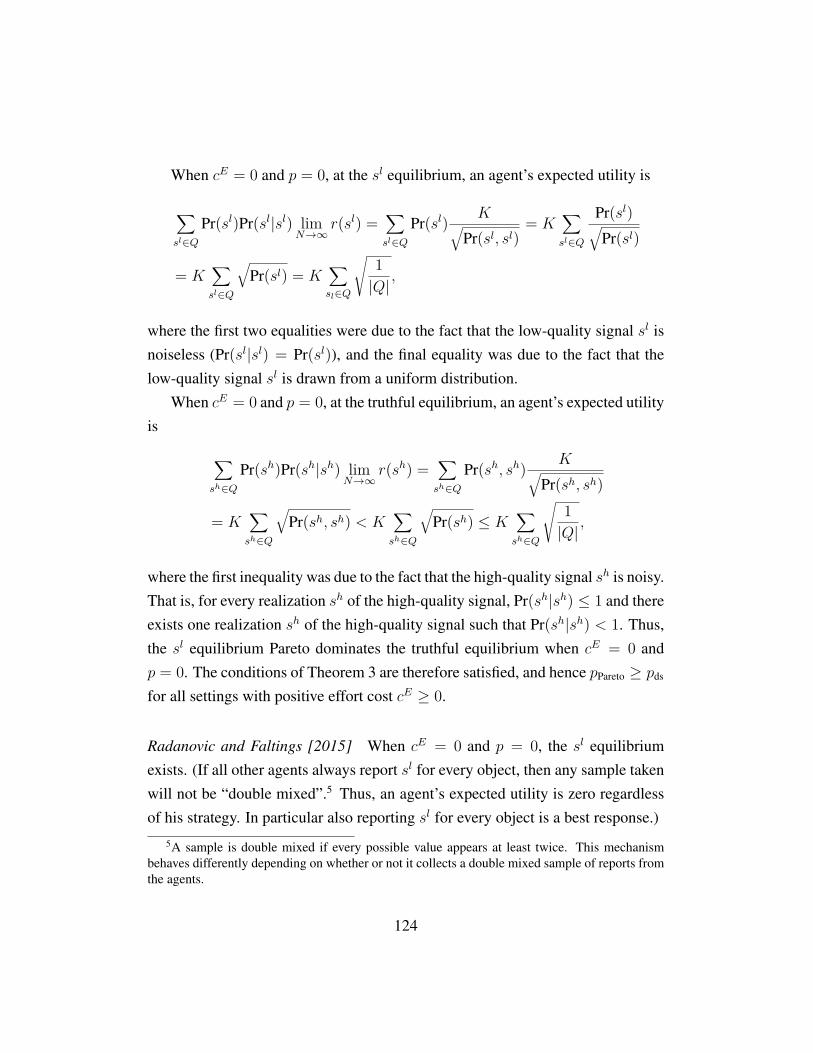
When cE = 0 and p = 0, at the sl equilibrium, an agent’s expected utility is

∑sl∈Q

Pr(sl)Pr(sl|sl) limN→∞

r(sl) =∑sl∈Q

Pr(sl) K√Pr(sl, sl)

= K∑sl∈Q

Pr(sl)√Pr(sl)

= K∑sl∈Q

√Pr(sl) = K

∑sl∈Q

√1|Q|

,

where the first two equalities were due to the fact that the low-quality signal sl isnoiseless (Pr(sl|sl) = Pr(sl)), and the final equality was due to the fact that thelow-quality signal sl is drawn from a uniform distribution.

When cE = 0 and p = 0, at the truthful equilibrium, an agent’s expected utilityis

∑sh∈Q

Pr(sh)Pr(sh|sh) limN→∞

r(sh) =∑sh∈Q

Pr(sh, sh) K√Pr(sh, sh)

= K∑sh∈Q

√Pr(sh, sh) < K

∑sh∈Q

√Pr(sh) ≤ K

∑sh∈Q

√1|Q|

,

where the first inequality was due to the fact that the high-quality signal sh is noisy.That is, for every realization sh of the high-quality signal, Pr(sh|sh) ≤ 1 and thereexists one realization sh of the high-quality signal such that Pr(sh|sh) < 1. Thus,the sl equilibrium Pareto dominates the truthful equilibrium when cE = 0 andp = 0. The conditions of Theorem 3 are therefore satisfied, and hence pPareto ≥ pds

for all settings with positive effort cost cE ≥ 0.

Radanovic and Faltings [2015] When cE = 0 and p = 0, the sl equilibriumexists. (If all other agents always report sl for every object, then any sample takenwill not be “double mixed”.5 Thus, an agent’s expected utility is zero regardlessof his strategy. In particular also reporting sl for every object is a best response.)

5A sample is double mixed if every possible value appears at least twice. This mechanismbehaves differently depending on whether or not it collects a double mixed sample of reports fromthe agents.

124

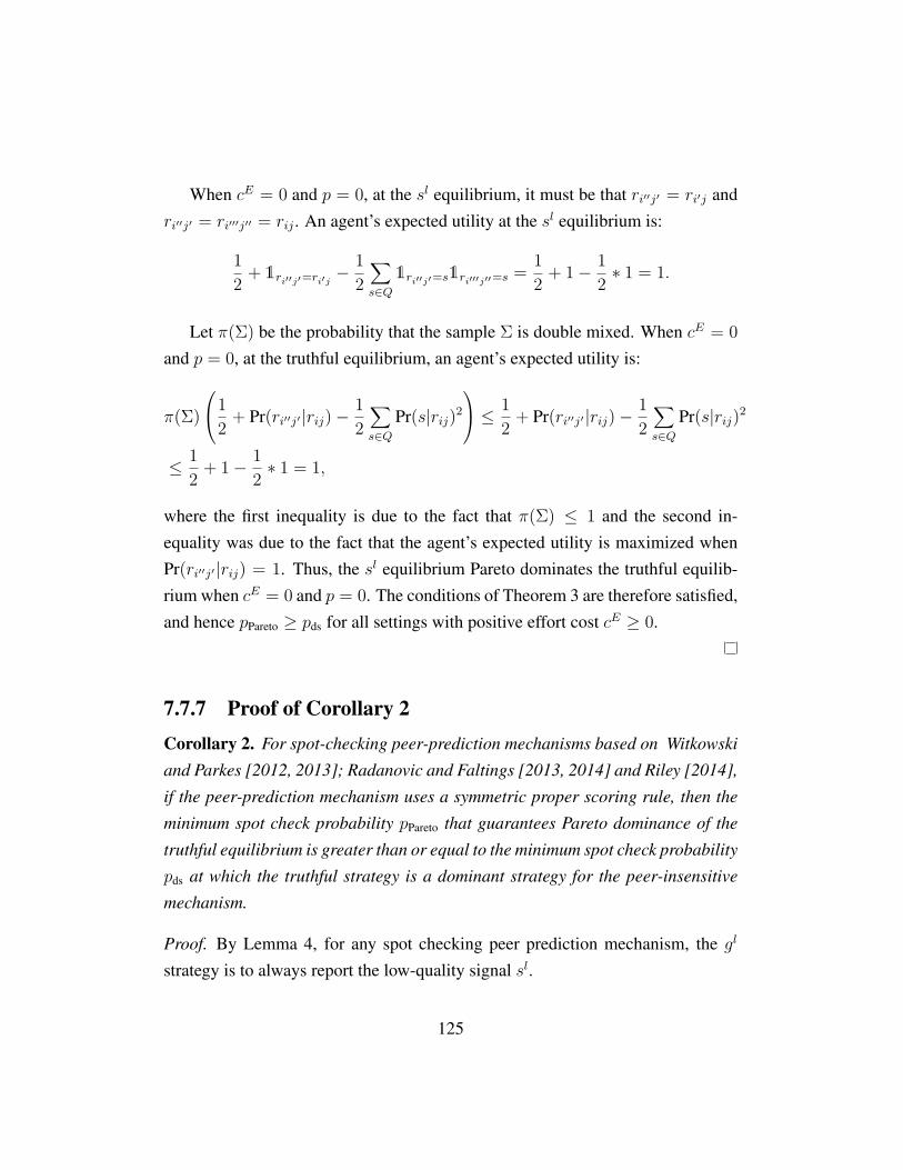
When cE = 0 and p = 0, at the sl equilibrium, it must be that ri′′j′ = ri′j andri′′j′ = ri′′′j′′ = rij . An agent’s expected utility at the sl equilibrium is:

12 + 1ri′′j′=ri′j

− 12∑s∈Q

1ri′′j′=s1ri′′′j′′=s = 12 + 1− 1

2 ∗ 1 = 1.

Let π(Σ) be the probability that the sample Σ is double mixed. When cE = 0and p = 0, at the truthful equilibrium, an agent’s expected utility is:

π(Σ)1

2 + Pr(ri′′j′|rij)−12∑s∈Q

Pr(s|rij)2

≤ 12 + Pr(ri′′j′|rij)−

12∑s∈Q

Pr(s|rij)2

≤ 12 + 1− 1

2 ∗ 1 = 1,

where the first inequality is due to the fact that π(Σ) ≤ 1 and the second in-equality was due to the fact that the agent’s expected utility is maximized whenPr(ri′′j′|rij) = 1. Thus, the sl equilibrium Pareto dominates the truthful equilib-rium when cE = 0 and p = 0. The conditions of Theorem 3 are therefore satisfied,and hence pPareto ≥ pds for all settings with positive effort cost cE ≥ 0.

7.7.7 Proof of Corollary 2Corollary 2. For spot-checking peer-prediction mechanisms based on Witkowski

and Parkes [2012, 2013]; Radanovic and Faltings [2013, 2014] and Riley [2014],

if the peer-prediction mechanism uses a symmetric proper scoring rule, then the

minimum spot check probability pPareto that guarantees Pareto dominance of the

truthful equilibrium is greater than or equal to the minimum spot check probability

pds at which the truthful strategy is a dominant strategy for the peer-insensitive

mechanism.

Proof. By Lemma 4, for any spot checking peer prediction mechanism, the gl

strategy is to always report the low-quality signal sl.

125

To verify that the conditions of Theorem 3 are satisfied, it suffices to verifythat when p = 0, the sl equilibrium of the peer prediction mechanism exists andPareto dominates the truthful equilibrium. We verify these two conditions for allof the listed peer prediction mechanisms below.

Let bs denote a belief report which predicts that signal s is observed with prob-ability 1, i.e. Pr(s) = 1 and Pr(s′) = 0,∀s′ ∈ Q, s′ 6= s. Let the sl equilibriumdenote the equilibrium where every agent’s signal report is sl and belief report isbsl .

For mathematical convenience, we assume that the scoring rule is symmetric

[Gneiting and Raftery, 2007]. That it, the reward for reporting a signal that ispredicted with probability 1 is the same regardless of the signal’s identity:

R(bs, s) = R(bs′ , s′), ∀s 6= s′.

This is a very mild condition that is satisfied by all standard scoring rules thatcompute rewards based purely on the predicted probabilities and the outcome,including the quadratic scoring rule and the log scoring rule.

For symmetric scoring rules, when p = 0, an agent’s expected score is maxi-mized by predicting bs when s is observed for any signal s ∈ Q.

Binary Robust BTS [Witkowski and Parkes, 2012, 2013] When cE = 0 and p =0, the sl equilibrium exists. (If all other agents report sl and bsl , then the bestbelief report for agent i is bsl . Moreover the best signal report for agent i is sl

which leads to a shadowed belief report of bsl .)When cE = 0 and p = 0, at the sl equilibrium, an agent’s expected utility is

R(bsl , sl)+R(ssl , sl). This is the maximum possible expected utility that an agentcan achieve because the proper scoring rule R is symmetric. Therefore, it mustbe greater than or equal to the agent’s expected utility at the truthful equilibriumwhen cE = 0 and p = 0.

126

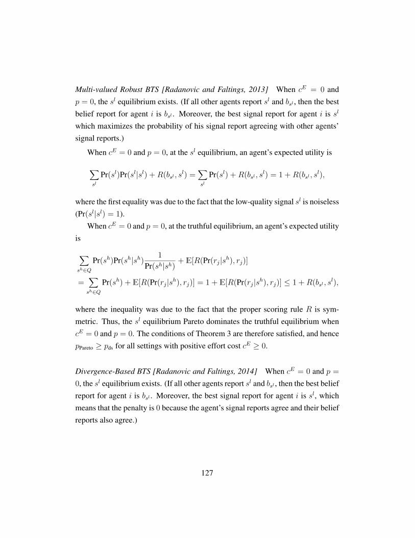
Multi-valued Robust BTS [Radanovic and Faltings, 2013] When cE = 0 andp = 0, the sl equilibrium exists. (If all other agents report sl and bsl , then the bestbelief report for agent i is bsl . Moreover, the best signal report for agent i is sl

which maximizes the probability of his signal report agreeing with other agents’signal reports.)

When cE = 0 and p = 0, at the sl equilibrium, an agent’s expected utility is

∑sl

Pr(sl)Pr(sl|sl) +R(bsl , sl) =∑sl

Pr(sl) +R(bsl , sl) = 1 +R(bsl , sl),

where the first equality was due to the fact that the low-quality signal sl is noiseless(Pr(sl|sl) = 1).

When cE = 0 and p = 0, at the truthful equilibrium, an agent’s expected utilityis

∑sh∈Q

Pr(sh)Pr(sh|sh) 1Pr(sh|sh) + E[R(Pr(rj|sh), rj)]

=∑sh∈Q

Pr(sh) + E[R(Pr(rj|sh), rj)] = 1 + E[R(Pr(rj|sh), rj)] ≤ 1 +R(bsl , sl),

where the inequality was due to the fact that the proper scoring rule R is sym-metric. Thus, the sl equilibrium Pareto dominates the truthful equilibrium whencE = 0 and p = 0. The conditions of Theorem 3 are therefore satisfied, and hencepPareto ≥ pds for all settings with positive effort cost cE ≥ 0.

Divergence-Based BTS [Radanovic and Faltings, 2014] When cE = 0 and p =0, the sl equilibrium exists. (If all other agents report sl and bsl , then the best beliefreport for agent i is bsl . Moreover, the best signal report for agent i is sl, whichmeans that the penalty is 0 because the agent’s signal reports agree and their beliefreports also agree.)

127

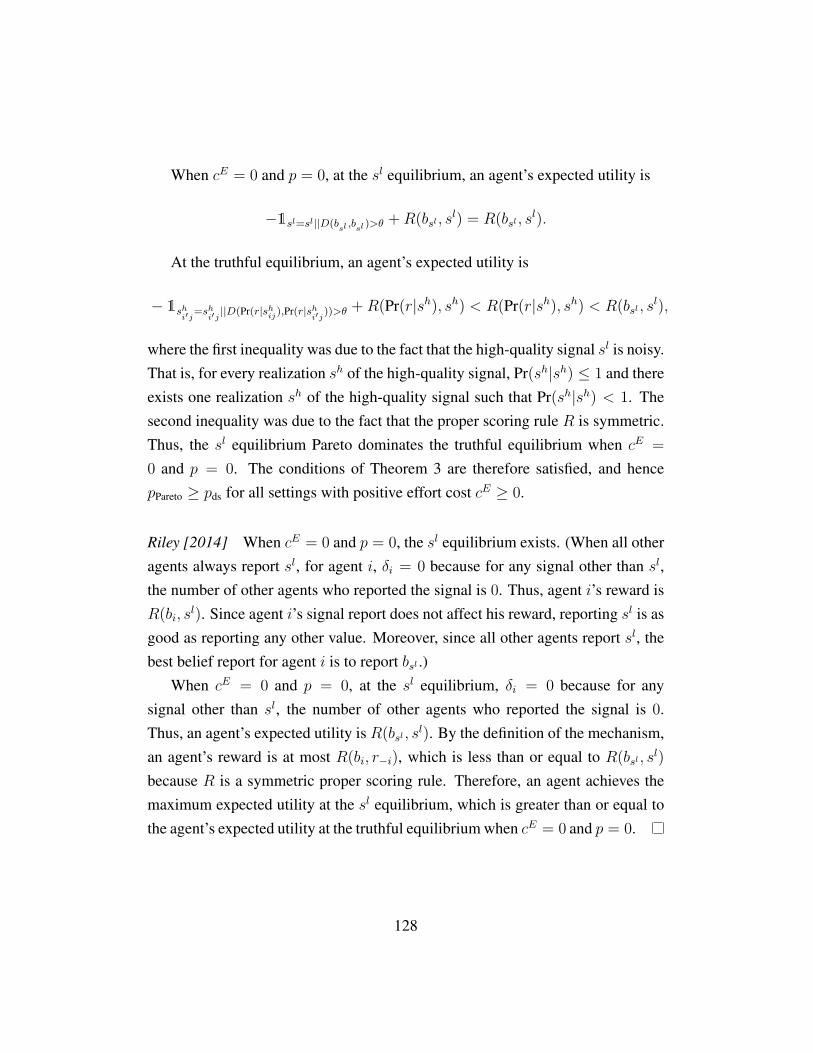
When cE = 0 and p = 0, at the sl equilibrium, an agent’s expected utility is

−1sl=sl||D(bsl ,bsl )>θ +R(bsl , sl) = R(bsl , sl).

At the truthful equilibrium, an agent’s expected utility is

− 1shi′j=sh

i′j ||D(Pr(r|shij),Pr(r|sh

i′j))>θ +R(Pr(r|sh), sh) < R(Pr(r|sh), sh) < R(bsl , sl),

where the first inequality was due to the fact that the high-quality signal sl is noisy.That is, for every realization sh of the high-quality signal, Pr(sh|sh) ≤ 1 and thereexists one realization sh of the high-quality signal such that Pr(sh|sh) < 1. Thesecond inequality was due to the fact that the proper scoring rule R is symmetric.Thus, the sl equilibrium Pareto dominates the truthful equilibrium when cE =0 and p = 0. The conditions of Theorem 3 are therefore satisfied, and hencepPareto ≥ pds for all settings with positive effort cost cE ≥ 0.

Riley [2014] When cE = 0 and p = 0, the sl equilibrium exists. (When all otheragents always report sl, for agent i, δi = 0 because for any signal other than sl,the number of other agents who reported the signal is 0. Thus, agent i’s reward isR(bi, sl). Since agent i’s signal report does not affect his reward, reporting sl is asgood as reporting any other value. Moreover, since all other agents report sl, thebest belief report for agent i is to report bsl .)

When cE = 0 and p = 0, at the sl equilibrium, δi = 0 because for anysignal other than sl, the number of other agents who reported the signal is 0.Thus, an agent’s expected utility is R(bsl , sl). By the definition of the mechanism,an agent’s reward is at most R(bi, r−i), which is less than or equal to R(bsl , sl)because R is a symmetric proper scoring rule. Therefore, an agent achieves themaximum expected utility at the sl equilibrium, which is greater than or equal tothe agent’s expected utility at the truthful equilibrium when cE = 0 and p = 0.

128

Chapter 8

Application: Mechanical TA

In the previous chapter, we started from a setting where the mechanism designerhad no access to ground truth whatsoever, and analyzed how one could improveits properties by adding minimal, costly access to ground truth. In this chapter, wepresent a case study that starts from a setting in which the mechanism designertypically observes ground truth for every single object (i.e., by marking everyassignment), and consider the symmetric question of how much costly access toground truth we can remove without damaging the mechanism’s goal of accurateevaluation.

Whereas the previous chapter took a theoretical approach, in this chapter wepresent a case study of a real-life peer grading scenario. In the previous chapter,we focused exclusively on the incentives problem, assuming that agents all had areliable high-quality signal. In practice, however, students have widely differingabilities. Thus, a major focus of this chapter is on validating that students (theagents) are competent graders (i.e., have access to a reliable signal).

8.1 IntroductionThis chapter describes our experience with software-supported, anonymous peergrading in a fourth year undergraduate course (“Computers and Society”). The

129

course focuses on reasoning critically about the importance and social implica-tions of computational advances. In earlier offerings of the course, students hadto write three essays: on the midterm, final, and for a term project. However,shorter and more frequent essay writing assignments are both a more effectiveway to teach writing skills [Seabrook et al., 2005], and provide more opportuni-ties to evaluate and improve writing skills and critical reasoning skills. Over thecourse of three offerings (2011, 2012, and 2013), we thus shifted to assigning stu-dents a total of 14 essays of about 300 words (11 weekly assignments, plus oneessay on the midterm exam and two essays on the final exam). Manually markingessays is very expensive in terms of teaching assistant (TA) time. Furthermore, itcan be difficult for students to learn to write such essays well. Peer grading offersa solution to both problems.

Peer grading is far from a new idea. However, students are often concernedthat the quality and fairness of the evaluation that they receive from peer gradingis lower than it would be from TAs [Robinson, 2001; Pare and Joordens, 2008;Walvoord et al., 2008]. Most systems (surveyed at the end of this article) attemptto address these concerns by evaluating the quality of the peer reviews in an auto-mated way, whether by reweighting reviews based on some criterion [Chapman,2001; Hamer et al., 2005], by “review the reviewer” schemes in which studentsrate the feedback they have received [Pare and Joordens, 2008; de Alfaro andShavlovsky, 2014b; Gehringer, 2001; Cho and Schunn, 2007b], by evaluating howclose a review is to the combined “consensus” grade for an assignment [de Alfaroand Shavlovsky, 2014b; Hamer et al., 2005], or by some combination of theseideas.

We wanted to use peer grading to make more efficient use of TAs, not to re-place them entirely. We thus designed a new system, dubbed “Mechanical TA.”1

Our system leverages (human) TAs in three ways. First, students start out in asupervised state, in which all of their reviews are marked by a TA. They are onlypromoted to an independent state when they demonstrate that they understand the

1Mechanical TA is freely available at http://www.cs.ubc.ca/∼jrwright/mta/.

130

grading rubric and are able to apply it competently. Second, students may use thesystem to appeal any peer grade that they consider unfair. (We reduce abuse ofthis feature by requiring a 100 word explanation of why a student believed that areview was unfair.) Finally, every independent review is eligible to be randomlyspot checked by a TA, who can retroactively mark a reviewer’s past reviews ifthey uncover a poor review. We found that students had surprisingly few concernsabout fairness in Mechanical TA, and believe that the visible involvement of hu-man TAs in marking assignments—especially in the early part of the class, whenmost students were supervised—was a major reason why.

Our system of random spot checks and appeals allows students to be persis-tently promoted. That is, once a student has been promoted, they can remainindependent for the remainder of the class (i.e., if they are not demoted again dueto a spot check or an appeal). This contrasts with systems such as Calibrated PeerReview (CPR) [Chapman, 2001], in which students’ review skills are retested atthe beginning of each assignment. The time required to complete such calibrationwas a source of complaints in one study of CPR [Walvoord et al., 2008].

Our implementation of calibration has a strong element of automated practicerather than just evaluation.2 To our knowledge, this is a unique feature of oursystem of calibration. Students receive immediate feedback about their perfor-mance on calibration essays, and may optionally choose to perform many morethan the required number of calibrations. In Section 8.4.2, we present our findingthat calibration practice significantly improved students’ review performance. InSection 8.3.3 we present evidence that it also improved students’ writing perfor-mance, as measured by exam scores.

We begin by describing our particular peer review model in detail in Sec-tion 8.2. We survey our experience with this model over three years (2011, 2012,2013) in Section 8.3, and compare some outcomes between different offeringsof the course, paying particular attention to the differences between the 2013

2Indeed, our evaluation suggests that this aspect was the main benefit offered by calibration inthe 2013 offering.

131

offering—which included automated calibration—and the previous two offerings.In Section 8.4 we analyze the data from the 2013 offering. In addition to show-ing that calibration practice improved students’ review skills, we also demonstratethat the persistent division of students into independent reviewers and supervisedreviewers was an effective strategy. After reviewing some related work in Sec-tion 8.5, we conclude in Section 8.6.

8.2 Peer Evaluation ModelIn brief, our peer review system works as follows. Students submit their essays asfree-form text in the Mechanical TA system.3 After the essay submission dead-line, each student is assigned three essays for double-blind peer review. After thedeadline for submitting reviews, each essay is assigned the median peer-reviewmark. Students can register a request for a TA to regrade their essay if they be-lieve that they received an unfair grade. The use of medians to compute gradesmeans that an appeal is only worthwhile if the student believes they received twounfair reviews.

A review consists of a configurable set of text fields and multiple-choice ques-tions. In our “Computers and Society” class, students were asked to rate eachessay on a scale of 0–5 along four dimensions—following a detailed rubric thatdescribed what an essay would look like to justify each score in each dimension—and provide a textual justification of their scores. The grade assigned to an essayby a review is the sum of the scores in each dimension. The full text of the rubricwe used is provided in Appendix A.

Mechanical TA implements a variant of the spot-checking scheme of Chap-ter 7. The mechanism automatically assigns a selection of essays to the TAs forspot checking, in which the TA reads the essay and evaluates its reviews. Theseessays are randomly selected. Unlike Chapter 7, where every review is selectedwith equal probability, Mechanical TA chooses some essays with higher proba-bility than others. For example, reviews that assign a high grade are more likely

3This makes it easy for us to check all essays for plagiarism using TurnItIn, which we do.

132

to be selected than reviews that assign a low grade. This addresses an incentiveasymmetry caused by the appeal system, since overly generous reviews are muchless likely to be appealed than overly harsh reviews.

8.2.1 Supervised and Independent ReviewersAs mentioned above, we classify students as either supervised or independent re-viewers. Every student begins as a supervised reviewer. Every essay that theyreview is also reviewed by a TA, and peer reviews are disregarded in this casefor the purpose of grading: supervised essays are assigned grades from TA re-views. Furthermore, supervised students’ reviews are also marked by TAs. Stu-dents are promoted from supervised to independent when their average reviewmarks crosses a configurable threshold. Once promoted to independent status, astudent automatically receives 100% on each of their reviews unless it is subse-quently checked by a TA as described earlier, in which case it is graded.

Supervised reviewers are assigned only the essays of other supervised review-ers; similarly, independent students are only matched with each other. This isimportant in terms of TA workload: indeed, it minimizes the number of essaysthat must be read by the TAs who evaluate the supervised reviewers’ reviews. Ifindependent and supervised students could review each others’ essays, then po-tentially every submitted essay would have at least one supervised reviewer andwould hence need to be read. Conversely (and for the same reason), our schememaximizes the number of essays that are fully peer graded.

8.2.2 CalibrationIn addition to giving them the opportunity to learn by reviewing the work of theirpeers, Mechanical TA also allows students to practice reviewing via calibration

essays. A calibration essay is an essay from a past offering of the course4 whichwas carefully evaluated by multiple TAs to establish a gold standard review. At

4Mechanical TA allows students to flag whether or not submissions may be used anonymously;we chose essays whose authors had permitted anonymous reuse.

133

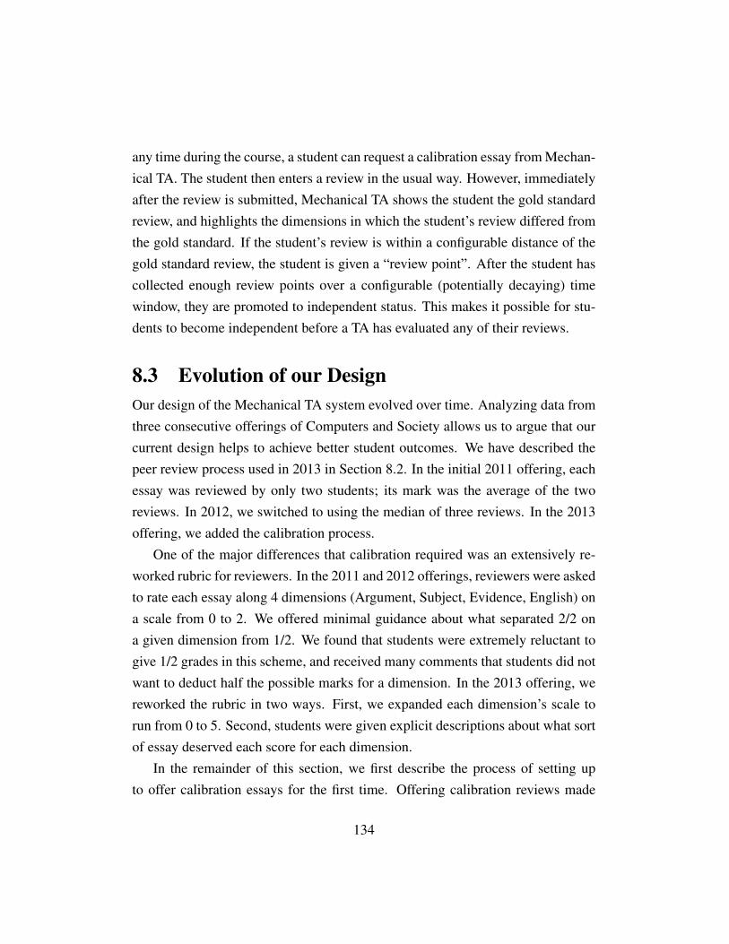
any time during the course, a student can request a calibration essay from Mechan-ical TA. The student then enters a review in the usual way. However, immediatelyafter the review is submitted, Mechanical TA shows the student the gold standardreview, and highlights the dimensions in which the student’s review differed fromthe gold standard. If the student’s review is within a configurable distance of thegold standard review, the student is given a “review point”. After the student hascollected enough review points over a configurable (potentially decaying) timewindow, they are promoted to independent status. This makes it possible for stu-dents to become independent before a TA has evaluated any of their reviews.

8.3 Evolution of our DesignOur design of the Mechanical TA system evolved over time. Analyzing data fromthree consecutive offerings of Computers and Society allows us to argue that ourcurrent design helps to achieve better student outcomes. We have described thepeer review process used in 2013 in Section 8.2. In the initial 2011 offering, eachessay was reviewed by only two students; its mark was the average of the tworeviews. In 2012, we switched to using the median of three reviews. In the 2013offering, we added the calibration process.

One of the major differences that calibration required was an extensively re-worked rubric for reviewers. In the 2011 and 2012 offerings, reviewers were askedto rate each essay along 4 dimensions (Argument, Subject, Evidence, English) ona scale from 0 to 2. We offered minimal guidance about what separated 2/2 ona given dimension from 1/2. We found that students were extremely reluctant togive 1/2 grades in this scheme, and received many comments that students did notwant to deduct half the possible marks for a dimension. In the 2013 offering, wereworked the rubric in two ways. First, we expanded each dimension’s scale torun from 0 to 5. Second, students were given explicit descriptions about what sortof essay deserved each score for each dimension.

In the remainder of this section, we first describe the process of setting upto offer calibration essays for the first time. Offering calibration reviews made

134

a substantial impact, both on students’ achievement, and on the workload for theTAs. In the final two subsections we compare 2013 to the earlier offerings by whenstudents were promoted to independent reviewer, and by exam performance.

8.3.1 Calibration SetupConstructing a library of calibration essays was a time-intensive process. Westarted by considering every essay from the previous offering that students hadflagged as available for anonymous reuse. We then hand-selected 27 candidateessays. Each of these essays was reviewed by the same four TAs. The reviewmarks were reconciled during in-person meetings, and every essay where the TAsreached consensus was selected as a calibration essay, whereas the other essayswere discarded.

One extremely valuable (and unintended) benefit of the process of creatingcalibration essays was calibrating the TAs themselves. With the exception of thelead TA, our course is run by a new contingent of TAs every year, most or all ofwhom have no particular past experience in evaluating essays. The meetings anddiscussions to determine marks for the calibration essays constituted an opportu-nity to give the TAs extensive extra training.

A one-time benefit of the initial process of creating calibration essays wasthat it pointed out opportunities to improve our rubric. The rubric went throughmultiple iterations during the process of calibrating the TAs, as they discoveredvarious ambiguities.

8.3.2 Independent ReviewersOne bottleneck in our original Mechanical TA design was that all students be-gin in the supervised pool, requiring extensive TA work at the beginning of term.One of our main motivations for introducing an automated calibration process toreduce this TA workload by encouraging students to be promoted to the inde-pendent pool before the first assignment was marked. We were unsuccessful inachieving this goal in our 2013 course offering: no students were promoted to

135

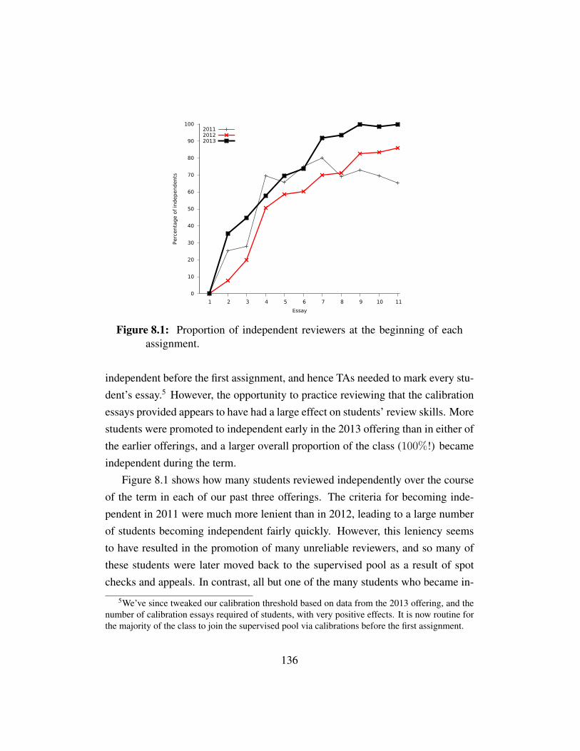
0

10

20

30

40

50

60

70

80

90

100

1 2 3 4 5 6 7 8 9 10 11

Perc

enta

ge o

f in

dep

end

ents

Essay

201120122013

Figure 8.1: Proportion of independent reviewers at the beginning of eachassignment.

independent before the first assignment, and hence TAs needed to mark every stu-dent’s essay.5 However, the opportunity to practice reviewing that the calibrationessays provided appears to have had a large effect on students’ review skills. Morestudents were promoted to independent early in the 2013 offering than in either ofthe earlier offerings, and a larger overall proportion of the class (100%!) becameindependent during the term.

Figure 8.1 shows how many students reviewed independently over the courseof the term in each of our past three offerings. The criteria for becoming inde-pendent in 2011 were much more lenient than in 2012, leading to a large numberof students becoming independent fairly quickly. However, this leniency seemsto have resulted in the promotion of many unreliable reviewers, and so many ofthese students were later moved back to the supervised pool as a result of spotchecks and appeals. In contrast, all but one of the many students who became in-

5We’ve since tweaked our calibration threshold based on data from the 2013 offering, and thenumber of calibration essays required of students, with very positive effects. It is now routine forthe majority of the class to join the supervised pool via calibrations before the first assignment.

136

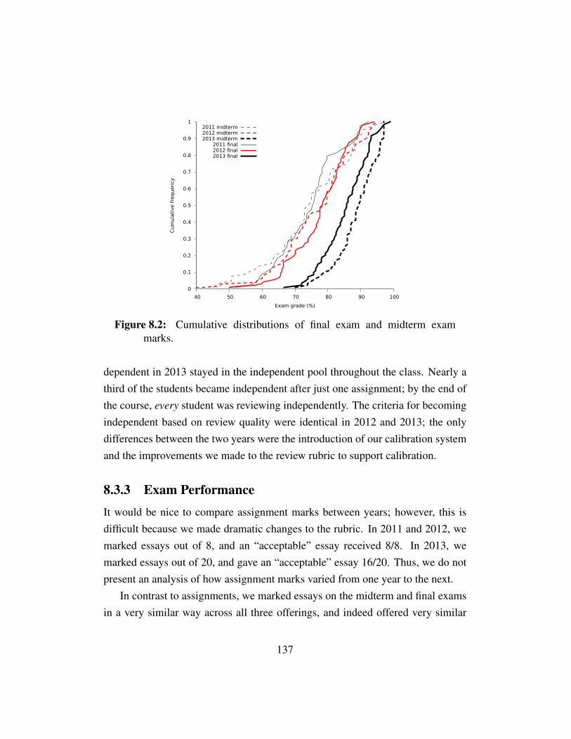
0

0.1

0.2

0.3

0.4

0.5

0.6

0.7

0.8

0.9

1

40 50 60 70 80 90 100

Cum

ula

tive f

req

uency

Exam grade (%)

2011 midterm2012 midterm2013 midterm

2011 final2012 final2013 final

Figure 8.2: Cumulative distributions of final exam and midterm exammarks.

dependent in 2013 stayed in the independent pool throughout the class. Nearly athird of the students became independent after just one assignment; by the end ofthe course, every student was reviewing independently. The criteria for becomingindependent based on review quality were identical in 2012 and 2013; the onlydifferences between the two years were the introduction of our calibration systemand the improvements we made to the review rubric to support calibration.

8.3.3 Exam PerformanceIt would be nice to compare assignment marks between years; however, this isdifficult because we made dramatic changes to the rubric. In 2011 and 2012, wemarked essays out of 8, and an “acceptable” essay received 8/8. In 2013, wemarked essays out of 20, and gave an “acceptable” essay 16/20. Thus, we do notpresent an analysis of how assignment marks varied from one year to the next.

In contrast to assignments, we marked essays on the midterm and final examsin a very similar way across all three offerings, and indeed offered very similar

137

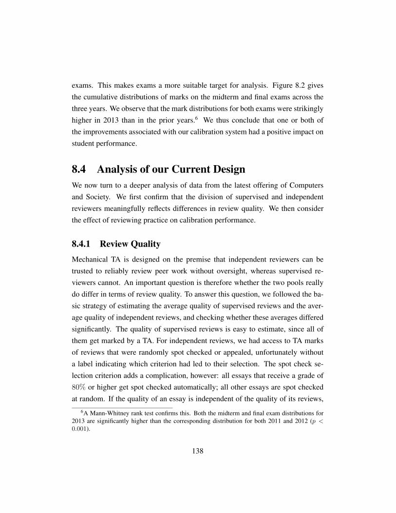
exams. This makes exams a more suitable target for analysis. Figure 8.2 givesthe cumulative distributions of marks on the midterm and final exams across thethree years. We observe that the mark distributions for both exams were strikinglyhigher in 2013 than in the prior years.6 We thus conclude that one or both ofthe improvements associated with our calibration system had a positive impact onstudent performance.

8.4 Analysis of our Current DesignWe now turn to a deeper analysis of data from the latest offering of Computersand Society. We first confirm that the division of supervised and independentreviewers meaningfully reflects differences in review quality. We then considerthe effect of reviewing practice on calibration performance.

8.4.1 Review QualityMechanical TA is designed on the premise that independent reviewers can betrusted to reliably review peer work without oversight, whereas supervised re-viewers cannot. An important question is therefore whether the two pools reallydo differ in terms of review quality. To answer this question, we followed the ba-sic strategy of estimating the average quality of supervised reviews and the aver-age quality of independent reviews, and checking whether these averages differedsignificantly. The quality of supervised reviews is easy to estimate, since all ofthem get marked by a TA. For independent reviews, we had access to TA marksof reviews that were randomly spot checked or appealed, unfortunately withouta label indicating which criterion had led to their selection. The spot check se-lection criterion adds a complication, however: all essays that receive a grade of80% or higher get spot checked automatically; all other essays are spot checkedat random. If the quality of an essay is independent of the quality of its reviews,

6A Mann-Whitney rank test confirms this. Both the midterm and final exam distributions for2013 are significantly higher than the corresponding distribution for both 2011 and 2012 (p <0.001).

138

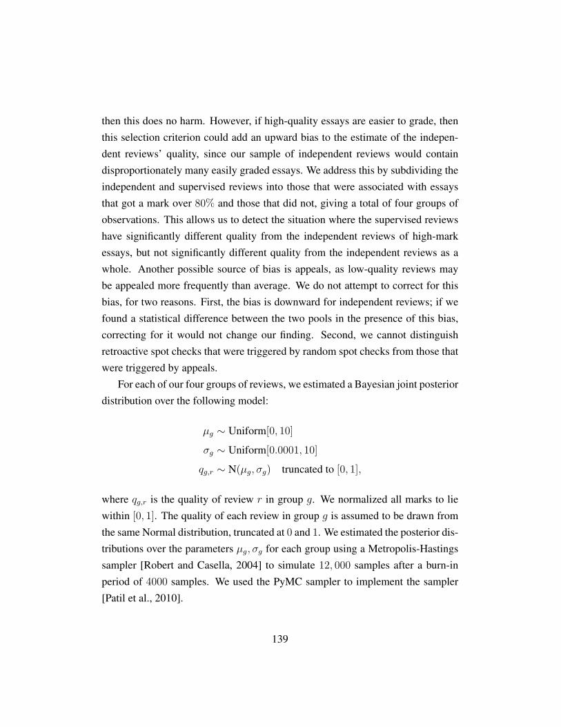
then this does no harm. However, if high-quality essays are easier to grade, thenthis selection criterion could add an upward bias to the estimate of the indepen-dent reviews’ quality, since our sample of independent reviews would containdisproportionately many easily graded essays. We address this by subdividing theindependent and supervised reviews into those that were associated with essaysthat got a mark over 80% and those that did not, giving a total of four groups ofobservations. This allows us to detect the situation where the supervised reviewshave significantly different quality from the independent reviews of high-markessays, but not significantly different quality from the independent reviews as awhole. Another possible source of bias is appeals, as low-quality reviews maybe appealed more frequently than average. We do not attempt to correct for thisbias, for two reasons. First, the bias is downward for independent reviews; if wefound a statistical difference between the two pools in the presence of this bias,correcting for it would not change our finding. Second, we cannot distinguishretroactive spot checks that were triggered by random spot checks from those thatwere triggered by appeals.

For each of our four groups of reviews, we estimated a Bayesian joint posteriordistribution over the following model:

µg ∼ Uniform[0, 10]

σg ∼ Uniform[0.0001, 10]

qg,r ∼ N(µg, σg) truncated to [0, 1],

where qg,r is the quality of review r in group g. We normalized all marks to liewithin [0, 1]. The quality of each review in group g is assumed to be drawn fromthe same Normal distribution, truncated at 0 and 1. We estimated the posterior dis-tributions over the parameters µg, σg for each group using a Metropolis-Hastingssampler [Robert and Casella, 2004] to simulate 12, 000 samples after a burn-inperiod of 4000 samples. We used the PyMC sampler to implement the sampler[Patil et al., 2010].

139

Figure 8.3 gives the cumulative posterior distribution over the average reviewquality for each group.7 The 95% central credible interval for each distribution isshown as a bar on the x-axis.8

We observe that there is no overlap between the central credible intervals ofeither independent group with either supervised group. This answers our ques-tion: we have strong evidence that independent reviewers perform higher qualityreviews.

We are also able to examine whether high-quality essays are easier to reviewwell. In both the independent and supervised groups, the quality of the reviewsof essays that received grades of at least 80% did indeed appear to be higher, al-though not substantially (nor significantly; the credible intervals for the above- andbelow-80% groups intersect). The effect was more pronounced in the supervisedgroup than in the independent group, although again not statistically significant.

8.4.2 Calibration PerformanceWe have described two benefits offered by calibration: assessing students’ re-view quality without TA intervention, and providing an opportunity for students topractice reviewing with immediate feedback. In this section, we evaluate whetherstudents benefit from such practice by asking whether students’ calibration marksimproved as they completed more calibration reviews.

We begin by plotting the performance of each calibration that was completed.We index calibrations by the time of promotion to the independent pool; that is,the last calibration review performed before a student was promoted is calibrationnumber 0, the calibration review completed just before that is calibration number-1, etc. We then perform a Bayesian linear regression by estimating the joint

7Due to the truncation of the Gaussian distributions to the interval [0, 1], this is not identical tothe posterior distribution of the µg parameter.

8A central credible interval is a Bayesian counterpart to a confidence interval. The true valueof a parameter lies within its 95% central credible interval with probability 0.95.

140

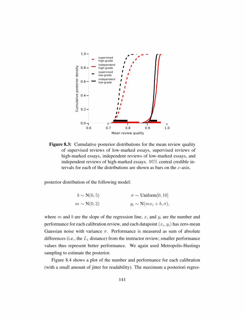
0.6 0.7 0.8 0.9 1.0

Mean review quality

0.0

0.2

0.4

0.6

0.8

1.0

Cum

ula

tive p

ost

eri

or

densi

ty

supervisedhigh-grade

independenthigh-grade

supervisedlow-grade

independentlow-grade

Figure 8.3: Cumulative posterior distributions for the mean review qualityof supervised reviews of low-marked essays, supervised reviews ofhigh-marked essays, independent reviews of low-marked essays, andindependent reviews of high-marked essays. 95% central credible in-tervals for each of the distributions are shown as bars on the x-axis.

posterior distribution of the following model:

b ∼ N(0, 5) σ ∼ Uniform[0, 10]

m ∼ N(0, 2) yi ∼ N(mxi + b, σ),

where m and b are the slope of the regression line, xi and yi are the number andperformance for each calibration review, and each datapoint (xi, yi) has zero-meanGaussian noise with variance σ. Performance is measured as sum of absolutedifferences (i.e., the L1 distance) from the instructor review; smaller performancevalues thus represent better performance. We again used Metropolis-Hastingssampling to estimate the posterior.

Figure 8.4 shows a plot of the number and performance for each calibration(with a small amount of jitter for readability). The maximum a posteriori regres-

141

Figure 8.4: Total deviations from gold standard review on calibration re-views, versus number of calibrations after promotion. The bold line isthe maximum a posteriori linear fit with Normal error. The gray linesare samples from the posterior predictive distribution of linear fits.

sion line is plotted as a bold line; this is the line whose slope and offset have thehighest posterior probability. To illustrate the range of possible fits, we also plotthe lines corresponding to 100 samples from the posterior distribution.

The MAP estimate of the slope is−0.085, with a 95% central credible intervalof [−0.104,−0.066]. The credible interval does not contain 0, so we concludethat students showed a significant improvement in their calibration performance asthey practiced. Our rubric grades essays out of 20, so a slope of−0.085 representsan average improvement of approximately 4% with each calibration.

8.5 Related WorkNow that we have described Mechanical TA in detail, we give a more thoroughsurvey of related work and describe how our own system differs. By far the mostwidely used online peer review system is Calibrated Peer Review (CPR) [Chap-

142

man, 2001; Robinson, 2001]. After submitting their own essays, students evaluatethree instructor-provided calibration essays of varying known quality. They thenanonymously review the essays of other students. Each review is weighted ac-cording to the reviewer’s performance on the calibration task. Reviewers whodo not pass the calibration task on the first two tries “flunk out” of the assign-ment and are not permitted to review at all. Review quality is further assessedby students’ reviewing other students’ reviews. The initial calibration essays areentirely for the purpose of evaluating students’ reviewing skill, and form a portionof the students’ grade. This contrasts with our calibration essays, which do notdirectly impact a student’s grade, and which allow students to practice reviewingin addition to demonstrating reviewing competence.

Kulkarni et al. [2014] combine algorithmic assessment of written answers withpeer review in a large online course. A learning algorithm first estimates both theassessment and its confidence in the assessment. These estimates are used todetermine how many peer reviews are required for a given item. Other studentsthen assess the peer reviews’ accuracy.

Mechanical TA focuses on evaluating the final version of an assignment. SWoRD[Cho and Schunn, 2007b], PRAZE [Mulder and Pearce, 2007], and CaptainTeach[Politz et al., 2014] allow students to incorporate feedback from peer reviews dur-ing the course of an assignment.

CrowdGrader [de Alfaro and Shavlovsky, 2014b] dynamically assigns reviewsto reviewers in an online fashion, in an attempt to provide an approximately equalnumber of reviews to each submission. Similarly to CPR, the quality of each re-view is assessed by comparing it to the “consensus” (trimmed average) review ofthe assignment; reviews that are further from the consensus are penalized. TheAropa system [Hamer et al., 2005] combines consistency scoring and weight-ing by reweighting reviews until the weights of the reviews are consistent withthe weighted average. Both systems thus assess review quality “automatically,”whereas Mechanical TA assesses review quality directly via TAs. Many othersystems use a “review the reviewer” system to evaluate review quality, in which

143

students rate the quality of the reviews they have received [Gehringer, 2001; Choand Schunn, 2007b; Mulder and Pearce, 2007; Pare and Joordens, 2008].

8.6 ConclusionsMechanical TA is a system designed to support a novel model of high-stakespeer grading, in which marks from trusted independent reviewers are binding (butcan be appealed), but marks from untrusted supervised reviewers are replaced bygrades from a TA. Students are promoted to independent status based on the qual-ity of their reviews, and after promotion they typically remain independent for theduration of the term. We have successfully used this system to set weekly essayassignments in a class of approximately 70 students. This would not be possibleif every assignment had to be graded by a TA, as essays are very time consum-ing to grade. We have focused here on grading essays, but our system is easilyapplicable to other domains such as coding assignments or code review.

The initial version of Mechanical TA employed a peer-insensitive spot-checkingmechanism (see Definition 15 in Chapter 7). A key driver of the theoretical inves-tigation in Chapter 7 was an attempt to make more efficient use of spot-checkingby incorporating peer-prediction into the spot checking mechanism. However,one of the main findings of that work was that peer-insensitive spot checkingmechanisms are actually more efficient at incentivizing truthful reporting thatpeer-prediction spot checking mechanisms. In this chapter, we instead focusedupon practical mechanisms for validating students’ competence through the su-pervised/independent distinction.

A major bottleneck in our peer review approach is that the first assignmentdoes require that TAs mark every submission along with all of the peer reviews.While we have found that TAs are willing to work hard at the beginning of termgiven assurances that they will subsequently have a much-reduced workload, thisbottleneck nevertheless limits the scalability of our system. We thus introducedcalibration reviews in the 2013 offering, in which students review carefully chosenassignments with known correct gold standard reviews constructed by the instruc-

144

tor and TAs. Each student receives automated feedback comparing their review tothe gold standard review, and if they match the gold standard closely enough onenough repetitions, they are automatically promoted to independent status. Thiscalibration mechanism has multiple goals. First, it aims to allow students to be-come independent before the first assignment, without TA intervention, therebyreducing TA workload on the first assignment. Second, it allows students to prac-tice the reviewing process, with immediate feedback about how well they did. Wedid not achieve the first goal in the 2013 course offering. Nevertheless, offeringstudents practice reviewing had a striking effect. Students in the 2013 offeringwere promoted sooner and received higher grades on roughly comparable examsthan those in the 2011 and 2012 offerings. Students’ average review performanceimproved by approximately 4% per attempted calibration essay.

One additional benefit of a calibration system is that it allows the systematictraining of TAs in how to mark according to subjective rubrics. (We described howour TAs benefited from constructing calibration questions; we’ve asked our 2014TAs to do the existing calibration exercises before the class starts.) We believethat this leads to higher quality marking by TAs and more consistency betweenTAs.

Calibrating reviewers before the first assignment is a key requirement for in-creasing the scalability of Mechanical TA’s peer review model. In the 2014 offer-ing subsequent to the years analyzed in this chapter, we modified the calibrationpromotion threshold based on data from the 2013 offering. This yielded a vastimprovement in how soon and how many students were moved to the supervisedpool. In the 2014 offering, over half of the students were admitted to the indepen-dent pool before the first assignment.

145

Bibliography

Agranov, M., Caplin, A., and Tergiman, C. (2010). The process of choice inguessing games. Social science working paper 1334r, California Institute ofTechnology. Available athttp://www.wordsmatter.caltech.edu/SSPapers/sswp1334R.pdf, accessed Feb.9, 2014. → pages 75

Altman, A., Bercovici-Boden, A., and Tennenholtz, M. (2006). Learning inone-shot strategic form games. In ECML 2006, 17th European Conference onMachine Learning, pages 6–17. → pages 37

Arad, A. (2012). The tennis coach problem: A game-theoretic and experimentalstudy. The BE Journal of Theoretical Economics, 12(1). → pages 75

Arad, A. and Rubinstein, A. (2009). Colonel Blotto’s top secret files. Workingpaper. Available athttp://www.dklevine.com/archive/refs4814577000000000432.pdf, accessedFeb. 9, 2014. → pages 75

Arad, A. and Rubinstein, A. (2012). The 11–20 money request game: A level-kreasoning study. The American Economic Review, 102(7):3561–3573. →pages 30, 75

Becker, T., Carter, M., and Naeve, J. (2005). Experts playing the traveler’sdilemma. Working paper, University of Hohenheim. → pages 9

Bengio, Y. (2009). Learning deep architectures for AI. Foundations and Trendsin Machine Learning, 2(1):1–127. → pages 5

Bengio, Y., Courville, A., and Vincent, P. (2013). Representation learning: Areview and new perspectives. IEEE Transactions on Pattern Analysis andMachine Intelligence, 35(8):1798–1828. → pages 78

146

Bishop, C. (2006). Pattern recognition and machine learning. Springer. →pages 11

Breitmoser, Y. (2012). Strategic reasoning in p-beauty contests. Games andEconomic Behavior, 75(2):555–569. → pages 36, 38

Burchardi, K. and Penczynski, S. (2011). Out of your mind: Eliciting individualreasoning in one shot games. Working paper, London School of Economics.→ pages 29, 30

Burchardi, K. and Penczynski, S. (2012). Out of your mind: Eliciting individualreasoning in one shot games. Working paper, London School of Economics.Available athttp://people.su.se/∼kburc/research/BurchardiPenczynski2012.pdf, accessedFeb. 9, 2014. → pages 58, 75, 76

Cabrera, S., Capra, C., and Gmez, R. (2007). Behavior in one-shot travelersdilemma games: model and experiments with advice. Spanish EconomicReview, 9(2):129–152. → pages 12

Camerer, C., Ho, T., and Chong, J. (2001). Behavioral game theory: Thinking,learning, and teaching. Nobel Symposium on Behavioral and ExperimentalEconomics. → pages 36, 38

Camerer, C., Ho, T., and Chong, J. (2004). A cognitive hierarchy model ofgames. Quarterly Journal of Economics, 119(3):861–898. → pages 10, 15,35, 36, 38, 40, 44, 45, 58, 70

Camerer, C. and Hua Ho, T. (1999). Experience-weighted attraction learning innormal form games. Econometrica, 67(4):827–874. → pages 12

Camerer, C., Nunnari, S., and Palfrey, T. R. (2011). Quantal response andnonequilibrium beliefs explain overbidding in maximum-value auctions.Working paper, California Institute of Technology. → pages 36, 38, 52

Camerer, C. and Thaler, R. H. (1995). Anomalies: Ultimatums, dictators andmanners. The Journal of Economic Perspectives, 9(2):209–219. → pages 62

Camerer, C. F. (2003). Behavioral Game Theory: Experiments in StrategicInteraction. Princeton University Press. → pages 3, 9

147

Capraro, V. (2013). A model of human cooperation in social dilemmas. PloSone, 8(8):e72427. → pages 12

Carvalho, D. and Santos-Pinto, L. (2010). A cognitive hierarchy model ofbehavior in endogenous timing games. Working paper, Universite deLausanne, Faculte des HEC, DEEP. → pages 44

Chapman, O. L. (2001). Calibrated Peer ReviewTM . → pages 130, 131, 142

Chawla, S., Hartline, J., and Nekipelov, D. (2014). Mechanism design for datascience. In Proceedings of the fifteenth ACM conference on Economics andcomputation, pages 711–712. → pages 2

Cho, K. and Schunn, C. D. (2007a). Scaffolded writing and rewriting in thediscipline: A web-based reciprocal peer review system. Computers &Education, 48(3):409–426. → pages 96

Cho, K. and Schunn, C. D. (2007b). Scaffolded writing and rewriting in thediscipline: A web-based reciprocal peer review system. Computers &Education, 48(3):409–426. → pages 130, 143, 144

Choi, S. (2012). A cognitive hierarchy model of learning in networks. Review ofEconomic Design, 16(2-3):215–250. → pages 44

Chong, J., Camerer, C., and Ho, T. (2005). Cognitive hierarchy: A limitedthinking theory in games. Experimental Business Research, Vol. III:Marketing, accounting and cognitive perspectives, pages 203–228. → pages29, 36, 38

Clark, C. and Storkey, A. J. (2015). Training deep convolutional neural networksto play go. In Proceedings of the 32nd International Conference on MachineLearning, ICML 2015, Lille, France, 6-11 July 2015, pages 1766–1774. →pages 79, 80

Cooper, D. and Van Huyck, J. (2003). Evidence on the equivalence of thestrategic and extensive form representation of games. Journal of EconomicTheory, 110(2):290–308. → pages 22, 23, 24, 25, 32

Costa-Gomes, M. and Crawford, V. (2006). Cognition and behavior intwo-person guessing games: An experimental study. American EconomicReview, 96(5):1737–1768. → pages 22, 38

148

Costa-Gomes, M., Crawford, V., and Broseta, B. (1998). Cognition and behaviorin normal-form games: an experimental study. Discussion paper 98-22,University of California, San Diego. → pages 22, 23, 25, 38

Costa-Gomes, M., Crawford, V., and Broseta, B. (2001). Cognition and behaviorin normal-form games: An experimental study. Econometrica,69(5):1193–1235. → pages 10, 14, 35, 38, 58, 60, 70

Costa-Gomes, M., Crawford, V., and Iriberri, N. (2009). Comparing models ofstrategic thinking in Van Huyck, Battalio, and Beil’s coordination games.Journal of the European Economic Association, 7(2-3):365–376. → pages 11,36, 38

Costa-Gomes, M. A. and Weizsacker, G. (2008). Stated beliefs and play innormal-form games. The Review of Economic Studies, 75(3):729–762. →pages 22, 23, 25, 36, 38

Crawford, V. and Iriberri, N. (2007a). Fatal attraction: Salience, naivete, andsophistication in experimental “hide-and-seek” games. American EconomicReview, 97(5):1731–1750. → pages 29, 30, 36, 38, 75

Crawford, V. and Iriberri, N. (2007b). Level-k auctions: Can a nonequilibriummodel of strategic thinking explain the winner’s curse and overbidding inprivate-value auctions? Econometrica, 75(6):1721–1770. → pages 30, 75

Dasgupta, A. and Ghosh, A. (2013). Crowdsourced judgement elicitation withendogenous proficiency. In Proceedings of the 22nd International Conferenceon the World Wide Web, pages 319–330. → pages 96, 97, 98, 101, 111, 121,122

de Alfaro, L. and Shavlovsky, M. (2014a). Crowdgrader: A tool forcrowdsourcing the evaluation of homework assignments. In Proceedings of the45th ACM Technical Symposium on Computer Science Education, pages415–420. → pages 96

de Alfaro, L. and Shavlovsky, M. (2014b). CrowdGrader: A tool forcrowdsourcing the evaluation of homework assignments. In Proceedings of the45th ACM Technical Symposium on Computer Science Education, SIGCSE’14, pages 415–420, New York, NY, USA. ACM. → pages 130, 143

149

Faltings, B., Jurca, R., Pu, P., and Tran, B. D. (2014). Incentives to counter biasin human computation. In Second AAAI Conference on Human Computationand Crowdsourcing. → pages 97

Faltings, B., Li, J. J., and Jurca, R. (2012). Eliciting truthful measurements froma community of sensors. In 3rd International Conference on the Internet ofThings, pages 47–54. → pages 96, 100, 101, 111, 121, 122

Frey, S. and Goldstone, R. (2011). Going with the group in a competitive gameof iterated reasoning. In 2011 Proceedings of the Cognitive Science Society,pages 1912–1917. → pages 44

Gao, X. A., Mao, A., Chen, Y., and Adams, R. P. (2014). Trick or treat: puttingpeer prediction to the test. In Proceedings of the Fifteenth ACM Conference onEconomics and Computation, pages 507–524. → pages 97

Gehringer, E. F. (2001). Electronic peer review and peer grading incomputer-science courses. ACM SIGCSE Bulletin, 33(1):139–143. → pages130, 144

Georganas, S., Healy, P. J., and Weber, R. (2010). On the persistence of strategicsophistication. Working paper, University of Bonn. → pages 38

Gilboa, I. and Schmeidler, D. (1989). Maxmin expected utility with non-uniqueprior. Journal of Mathematical Economics, 18(2):141–153. → pages 2

Gill, J. (2002). Bayesian methods: A social and behavioral sciences approach.CRC press. → pages 42

Gneiting, T. and Raftery, A. E. (2007). Strictly proper scoring rules, prediction,and estimation. Journal of the American Statistical Association,102(477):359–378. → pages 126

Goeree, J. K. and Holt, C. A. (2001). Ten little treasures of game theory and tenintuitive contradictions. American Economic Review, 91(5):1402–1422. →pages 3, 9, 22, 23, 25, 30, 32

Goeree, J. K. and Holt, C. A. (2004). A model of noisy introspection. Gamesand Economic Behavior, 46(2):365–382. → pages 10, 18, 35, 36, 38

Goldstein, A. A. (1964). Convex programming in Hilbert space. Bull. Amer.Math. Soc., 70(5):709–710. → pages 88

150

Goodie, A. S., Doshi, P., and Young, D. L. (2012). Levels of theory-of-mindreasoning in competitive games. Journal of Behavioral Decision Making,25(1):95–108. → pages 44

Hahn, P. R., Lum, K., and Mela, C. (2010). A semiparametric model forassessing cognitive hierarchy theories of beauty contest games. Workingpaper, Duke University. → pages 36, 38

Hamer, J., Ma, K. T. K., and Kwong, H. H. F. (2005). A method of automaticgrade calibration in peer assessment. In Proceedings of the 7th AustralasianConference on Computing Education - Volume 42, ACE ’05, pages 67–72,Darlinghurst, Australia, Australia. Australian Computer Society, Inc. → pages96, 130, 143

Hansen, N. and Ostermeier, A. (2001). Completely derandomized self-adaptationin evolution strategies. Evolutionary Computation, 9(2):159–195. → pages 26

Hargreaves Heap, S., Rojo Arjona, D., and Sugden, R. (2014). How portable islevel-0 behavior? A test of level-k theory in games with non-neutral frames.Econometrica, 82(3):1133–1151. → pages 76

Haruvy, E. and Stahl, D. (2007). Equilibrium selection and bounded rationalityin symmetric normal-form games. Journal of Economic Behavior andOrganization, 62(1):98–119. → pages 22, 24, 25

Haruvy, E., Stahl, D., and Wilson, P. (1999). Evidence for optimistic andpessimistic behavior in normal-form games. Economics Letters,63(3):255–259. → pages 38

Haruvy, E., Stahl, D., and Wilson, P. (2001). Modeling and testing forheterogeneity in observed strategic behavior. Review of Economics andStatistics, 83(1):146–157. → pages 22, 23, 25, 29, 38

Ho, T., Camerer, C., and Weigelt, K. (1998). Iterated dominance and iterated bestresponse in experimental “p-beauty contests”. American Economic Review,88(4):947–969. → pages 10, 11

Hutter, F., Hoos, H. H., and Leyton-Brown, K. (2010). Sequential model-basedoptimization for general algorithm configuration (extended version). TechnicalReport TR-2010-10, University of British Columbia, Department of Computer

151

Science. Available online:http://www.cs.ubc.ca/˜hutter/papers/10-TR-SMAC.pdf. → pages 67

Hutter, F., Hoos, H. H., and Leyton-Brown, K. (2011). Sequential model-basedoptimization for general algorithm configuration. In Proc. of LION-5, page507523. → pages 67

Hutter, F., Hoos, H. H., and Leyton-Brown, K. (2012). Parallel algorithmconfiguration. In Proc. of LION-6, pages 55–70. → pages 67

Jiang, A. X., Leyton-Brown, K., and Bhat, N. A. (2011). Action-graph games.Games and Economic Behavior, 71(1):141–173. → pages 22

John, L. K., Loewenstein, G., and Prelec, D. (2012). Measuring the prevalence ofquestionable research practices with incentives for truth telling. PsychologicalScience, 23(5):524–532. → pages 97

Jurca, R. and Faltings, B. (2005). Enforcing truthful strategies in incentivecompatible reputation mechanisms. Internet and Network Economics, pages268–277. → pages 98

Jurca, R. and Faltings, B. (2009). Mechanisms for making crowds truthful.Journal of Artificial Intelligence Research, 34(1):209. → pages 96, 97, 103

Kamble, V., Shah, N., Marn, D., Parekh, A., and Ramachandran, K. (2015).Truth serums for massively crowdsourced evaluation tasks. arXiv preprintarXiv:1507.07045. → pages 96, 97, 101, 111, 121, 123

Kearns, M., Littman, M. L., and Singh, S. (2001). Graphical models for gametheory. In Proceedings of the Seventeenth Conference on Uncertainty inArtificial Intelligence, pages 253–260. → pages 22

Koller, D. and Milch, B. (2001). Multi-agent influence diagrams for representingand solving games. In IJCAI, pages 1027–1036. → pages 22

Kong, Y., Schoenebeck, G., and Ligett, K. (2016). Putting peer prediction underthe micro (economic) scope and making truth-telling focal. arXiv preprintarXiv:1603.07319. → pages 96, 103

Kulkarni, C. E., Socher, R., Bernstein, M. S., and Klemmer, S. R. (2014).Scaling short-answer grading by combining peer assessment with algorithmic

152

scoring. In Proceedings of the First ACM Conference on Learning @ Scale,pages 99–108. → pages 96, 143

LeCun, Y., Bengio, Y., and Hinton, G. (2015). Deep learning. Nature,521(7553):436–444. → pages 79

LeCun, Y., Bottou, L., Bengio, Y., and Haffner, P. (1998). Gradient-basedlearning applied to document recognition. Proceedings of the IEEE,86(11):2278–2324. → pages 6

Lin, M., Chen, Q., and Yan, S. (2013). Network in network. CoRR,abs/1312.4400. → pages 80, 88

McKelvey, R., McLennan, A., and Turocy, T. (2007). Gambit: Software tools forgame theory, version 0.2007. 01.30. → pages 26

McKelvey, R. and Palfrey, T. (1995). Quantal response equilibria for normalform games. Games and Economic Behavior, 10(1):6–38. → pages 10, 13, 35,38

Miller, N., Resnick, P., and Zeckhauser, R. (2005). Eliciting informativefeedback: The peer-prediction method. Management Science,51(9):1359–1373. → pages 96, 103

Morgan, J. and Sefton, M. (2002). An experimental investigation of unprofitablegames. Games and Economic Behavior, 40(1):123–146. → pages 36, 38

Mulder, R. A. and Pearce, J. M. (2007). PRAZE: Innovating teaching throughonline peer review. In Proceedings of the 24th Annual Conference of theAustralasian Society for Computers in Learning in Tertiary Education. →pages 143, 144

Nagel, R. (1995). Unraveling in guessing games: An experimental study.American Economic Review, 85(5):1313–1326. → pages 10, 35, 58, 75

Neal, R. M. (2001). Annealed importance sampling. Statistics and Computing,11(2):125–139. → pages 42

Osborne, M. J. and Rubinstein, A. (1998). Games with procedurally rationalplayers. American Economic Review, 88(4):834–847. → pages 12

153

Pare, D. E. and Joordens, S. (2008). Peering into large lectures: examining peerand expert mark agreement using peerScholar, an online peer assessment tool.Journal of Computer Assisted Learning, 24(6):526–540. → pages 96, 130, 144

Patil, A., Huard, D., and Fonnesbeck, C. (2010). PyMC: Bayesian stochasticmodelling in Python. Journal of Statistical Software, 35(1). → pages 43, 139

Politz, J. G., Patterson, D., Krishnamurthi, S., and Fisler, K. (2014).CaptainTeach: Multi-stage, in-flow peer review for programming assignments.In ACM SIGCSE Conference on Innovation and Technology in ComputerScience Education. → pages 143

Prelec, D. (2004). A Bayesian truth serum for subjective data. science,306(5695):462–466. → pages 96, 103

Rabin, M. (2000). Risk aversion and expected-utility theory: A calibrationtheorem. Econometrica, pages 1281–1292. → pages 3

Radanovic, G. and Faltings, B. (2013). A robust Bayesian truth serum fornon-binary signals. In Proceedings of the 27th AAAI Conference on ArtificialIntelligence, pages 833–839. → pages 96, 102, 104, 112, 125, 127

Radanovic, G. and Faltings, B. (2014). Incentives for truthful informationelicitation of continuous signals. In Twenty-Eighth AAAI Conference onArtificial Intelligence. → pages 96, 102, 103, 104, 112, 125, 127

Radanovic, G. and Faltings, B. (2015). Incentives for subjective evaluations withprivate beliefs. In Twenty-Ninth AAAI Conference on Artificial Intelligence. →pages 97, 101, 102, 111, 121, 124

Rey-Biel, P. (2009). Equilibrium play and best response to (stated) beliefs innormal form games. Games and Economic Behavior, 65(2):572–585. →pages 38

Riley, B. (2014). Minimum truth serums with optional predictions. InProceedings of the 4th Workshop on Social Computing and User GeneratedContent. → pages 96, 102, 103, 104, 112, 125, 128

Robert, C. P. and Casella, G. (2004). Monte Carlo statistical methods. SpringerVerlag. → pages 42, 139

154

Robinson, R. (2001). Calibrated Peer ReviewTM an application to increasestudent reading & writing skills. The American Biology Teacher, 63(7):pp.474–476+478–480. → pages 130, 143

Rogers, B. W., Palfrey, T. R., and Camerer, C. F. (2009). Heterogeneous quantalresponse equilibrium and cognitive hierarchies. Journal of Economic Theory,144(4):1440–1467. → pages 10, 12, 16, 22, 24, 25, 29, 32, 36, 37, 38

Savage, L. (1951). The theory of statistical decision. Journal of the AmericanStatistical Association, 46(253):55–67. → pages 61

Schmidhuber, J. (2015). Deep learning in neural networks: An overview. NeuralNetworks, 61:85–117. → pages 80

Seabrook, R., Brown, G. D., and Solity, J. (2005). Distributed and massedpractice: from laboratory to classroom. Applied Cognitive Psychology,19(1):107–122. → pages 130

Selten, R. and Buchta, J. (1994). Experimental sealed bid first price auctionswith directly observed bid functions. Discussion paper B-270, University ofBonn. → pages 12

Selten, R. and Chmura, T. (2008). Stationary concepts for experimental2× 2-games. American Economic Review, 98(3):938–966. → pages 12

Shaw, A. D., Horton, J. J., and Chen, D. L. (2011). Designing incentives forinexpert human raters. In Proceedings of the ACM 2011 Conference onComputer Supported Cooperative Work, pages 275–284. → pages 97

Shnayder, V., Agarwal, A., Frongillo, R., and Parkes, D. C. (2016). Informedtruthfulness in multi-task peer prediction. arXiv preprint arXiv:1603.03151.→ pages 96, 97, 101, 112, 121, 122

Shoham, Y. and Leyton-Brown, K. (2008). Multiagent Systems: Algorithmic,Game-theoretic, and Logical Foundations. Cambridge University Press. →pages 26

Silver, D., Huang, A., Maddison, C. J., Guez, A., Sifre, L., van den Driessche,G., Schrittwieser, J., Antonoglou, I., Panneershelvam, V., Lanctot, M.,Dieleman, S., Grewe, D., Nham, J., Kalchbrenner, N., Sutskever, I., Lillicrap,T., Leach, M., Kavukcuoglu, K., Graepel, T., and Hassabis, D. (2016).

155

Mastering the game of Go with deep neural networks and tree search. Nature,529:484–503. → pages 80

Stahl, D. and Haruvy, E. (2008). Level-n bounded rationality and dominatedstrategies in normal-form games. Journal of Economic Behavior andOrganization, 66(2):226–232. → pages 22, 24, 25, 38

Stahl, D. and Wilson, P. (1994). Experimental evidence on players’ models ofother players. Journal of Economic Behavior and Organization,25(3):309–327. → pages 10, 11, 16, 17, 22, 23, 24, 25, 29, 35, 38, 44, 45, 58

Stahl, D. and Wilson, P. (1995). On players’ models of other players: Theory andexperimental evidence. Games and Economic Behavior, 10(1):218–254. →pages 10, 22, 23, 25, 29, 36, 38

Thaler, R. H. (1988). Anomalies: The Ultimatum Game. The Journal ofEconomic Perspectives, 2(4):195–206. → pages 62

Turocy, T. (2005). A dynamic homotopy interpretation of the logistic quantalresponse equilibrium correspondence. Games and Economic Behavior,51(2):243–263. → pages 13

Tversky, A. and Kahneman, D. (1992). Advances in prospect theory: Cumulativerepresentation of uncertainty. Journal of Risk and Uncertainty, 5(4):297–323.→ pages 2

Von Neumann, J. and Morgenstern, O. (1944). Theory of Games and EconomicBehavior. Princeton University Press. → pages 14

Waggoner, B. and Chen, Y. (2014). Output agreement mechanisms and commonknowledge. In Proceedings of the 2nd AAAI Conference on HumanComputation and Crowdsourcing. → pages 96, 97, 101, 111, 121

Walvoord, M. E., Hoefnagels, M. H., Gaffin, D. D., Chumchal, M. M., and Long,D. A. (2008). An analysis of Calibrated Peer Review (CPR) in a sciencelecture classroom. Journal of College Science Teaching, 37(4):66. → pages130, 131

Weizsacker, G. (2003). Ignoring the rationality of others: Evidence fromexperimental normal-form games. Games and Economic Behavior,44(1):145–171. → pages 10, 12, 38

156

Wilson, R. (1987). Game-theoretic approaches to trading processes. In Advancesin Economic Theory: Fifth World Congress, pages 33–77. → pages 100

Witkowski, J., Bachrach, Y., Key, P., and Parkes, D. C. (2013). Dwelling on thenegative: Incentivizing effort in peer prediction. In Proceedings of the 1stAAAI Conference on Human Computation and Crowdsourcing. → pages 96,100, 101, 111, 121

Witkowski, J. and Parkes, D. C. (2012). A robust Bayesian truth serum for smallpopulations. In Proceedings of the 26th AAAI Conference on ArtificialIntelligence. → pages 96, 102, 104, 112, 125, 126

Witkowski, J. and Parkes, D. C. (2013). Learning the prior in minimal peerprediction. In Proceedings of the 3rd Workshop on Social Computing andUser Generated Content at the ACM Conference on Electronic Commerce,page 14. → pages 96, 97, 102, 104, 112, 125, 126

Witten, I. H. and Frank, E. (2000). Data Mining: Practical Machine LearningTools and Techniques with Java Implementations. Morgan Kaufmann. →pages 22

Wright, J. R. and Leyton-Brown, K. (2010). Beyond equilibrium: Predictinghuman behavior in normal-form games. In Proceedings of the Twenty-FourthAAAI Conference on Artificial Intelligence, pages 901–907. → pages iv

Wright, J. R. and Leyton-Brown, K. (2012). Behavioral game-theoretic models:A Bayesian framework for parameter analysis. In Proceedings of the 11thInternational Conference on Autonomous Agents and Multiagent Systems,volume 2, pages 921–928. → pages iv

Wright, J. R. and Leyton-Brown, K. (2014). Level-0 meta-models for predictinghuman behavior in games. In Proceedings of the Fifteenth ACM Conference onEconomics and Computation, pages 857–874. → pages iv, 66

Wright, J. R., Thornton, C., and Leyton-Brown, K. (2015). Mechanical TA:Partially automated high-stakes peer grading. In Proceedings of the 46th ACMTechnical Symposium on Computer Science Education, pages 96–101. →pages v

157

Zhang, P. and Chen, Y. (2014). Elicitability and knowledge-free elicitation withpeer prediction. In Proceedings of the 2014 International Conference onAutonomous Agents and Multiagent Systems, pages 245–252. → pages 96, 103

158

Appendices

159

Appendix A

CPSC 430 2014 grading rubric

For each of the following four dimensions, choose the option that best describesthe essay:

EnglishWas the essay presented CLEARLY AND IN CORRECT ENGLISH?

0. Completely indecipherable.

1. Very difficult to understand.

2. Weak presentation; errors that impede understanding.

3. Mostly correct, fairly clear writing.

4. Clear and correct writing.

5. Very clear and correct writing.

160

Argument structureWas the essay WELL STRUCTURED, stating a thesis, supporting it with argu-ment(s) that are clearly related to this point and (if relevant) distinct from oneanother, and linking these arguments in a logical way?

0. It is unclear what this essay is arguing.

1. It is apparent what is being argued, but much of the reasoning is unsound,unclear, or unrelated.

2. The thesis is clearly stated, and some claims support the thesis, but othersare irrelevant and/or redundant.

3. All claims lend support to a clearly stated thesis, but they are insufficientlydistinct and/or poorly linked together.

4. All claims lend support to a clearly stated thesis, which in turn relates ap-propriately to the question asked. The claims are distinct from one anotherand build well on each other in a logical progression.

5. Very well structured: the thesis is clear and well related to the questionasked; the logical structure of arguments does an excellent job of supportingthis thesis.

161

CaseDid the essay do a GOOD JOB OF MAKING ITS CASE, choosing relevant ar-guments, backing them up with evidence and examples at an appropriate level ofdetail, and responding to contrary views as appropriate?

0. Claims are asserted with no further support, or not asserted at all.

1. The essay stated many facts about the topic in question, but there is not aclear separation between argument and evidence.

2. The essay makes recognizable arguments and backs them up with evidence,but relevance and/or level of detail are very inappropriate and/or extremelyrelevant contrary views are disregarded.

3. Arguments are clearly stated and generally support the thesis; these argu-ments are backed up with generally relevant evidence at a broadly appropri-ate level of detail. No extremely relevant contrary view undermines thesearguments, though such arguments may or may not be explicitly addressedin the essay.

4. All claims are grounded in relevant and specific arguments at an appropriatelevel of detail; some attempt is made to respond to alternate points of view.

5. Whether or not I personally agree with the essay’s thesis, it makes a com-pelling argument for its point of view. Arguments are very relevant, backedup with evidence at an appropriate level of detail, and (within space avail-able) responses are offered to obvious objections.

162

Subject matterDid the essay demonstrate a good UNDERSTANDING OF THE COURSE’SSUBJECT MATTER, including both the topic and the wider context?

0. Profound and fundamental misunderstanding of the subject matter.

1. Poor understanding of the subject matter; major errors.

2. Factual errors that substantially undermined the essay’s main point.

3. Generally correct understanding, but minor errors and/or errors of omission(failure to introduce important facts).

4. Correct understanding, generally balanced presentation at an appropriatelevel of detail.

5. Insightful understanding, creative and balanced use of the course’s subjectmatter.

163