Modeling Flows in Irrigation Distribution Networks – Model Description and Prototype

Yanbo Huang, Associate Research Scientist Guy Fipps, Professor

Biological and Agricultural Engineering Department, Texas A&M University

Written for presentation at the 2003 ASAE Annual International Meeting

Sponsored by ASAE Riviera Hotel and Convention Center

Las Vegas, Nevada, USA 27- 30 July 2003

Abstract. Efforts are underway to rehabilitate the irrigation districts of the Rio Grande River Basin in Texas. Distribution network models are needed to help prioritize and analyze various rehabilitation options, as well as to scientifically quantify irrigation water demands, usages, and losses, and to help manage gate automation. This paper reports on the methodology of a simulation model prototype for water flow in irrigation distribution networks. A description of the prototype model components and verification of the algorithms for open-channels and pipelines are presented. In order to enhance spatial data analysis, GIS data sources are incorporated. This GIS-based model prototype will play an important role in planning, analysis and development for water quantification and modernization of irrigation systems.

Keywords. LRGV, Irrigation Distribution Networks, Open-Channel, Pipeline, Model Prototype, GIS integration.

The authors are solely responsible for the content of this technical presentation. The technical presentation does not necessarily reflect the official position of the American Society of Agricultural Engineers (ASAE), and its printing and distribution does not constitute an endorsement of views which may be expressed. Technical presentations are not subject to the formal peer review process by ASAE editorial committees; therefore, they are not to be presented as refereed publications. Citation of this work should state that it is from an ASAE meeting paper EXAMPLE: Author's Last Name, Initials. 2003. Title of Presentation. ASAE Paper No. 03xxxx. St. Joseph, Mich.: ASAE. For information about securing permission to reprint or reproduce a technical presentation, please contact ASAE at hq@asae.org or 269-429-0300 (2950 Niles Road, St. Joseph, MI 49085-9659 USA).

Paper Number: 032146An ASAE Meeting Presentation

2

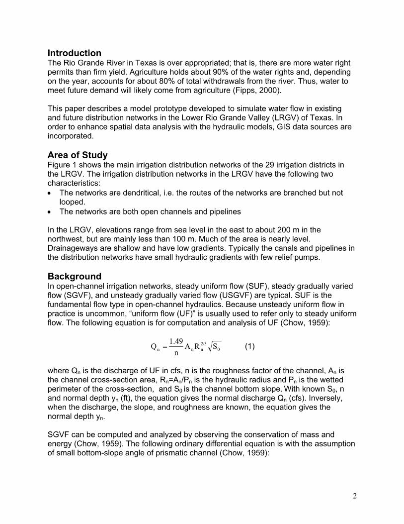
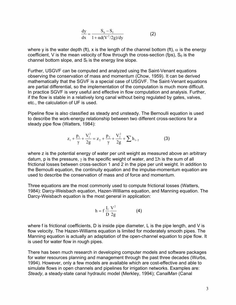
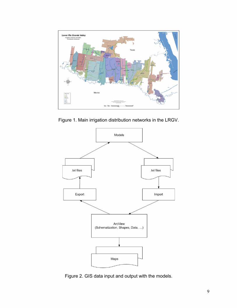
Introduction The Rio Grande River in Texas is over appropriated; that is, there are more water right permits than firm yield. Agriculture holds about 90% of the water rights and, depending on the year, accounts for about 80% of total withdrawals from the river. Thus, water to meet future demand will likely come from agriculture (Fipps, 2000). This paper describes a model prototype developed to simulate water flow in existing and future distribution networks in the Lower Rio Grande Valley (LRGV) of Texas. In order to enhance spatial data analysis with the hydraulic models, GIS data sources are incorporated. Area of Study Figure 1 shows the main irrigation distribution networks of the 29 irrigation districts in the LRGV. The irrigation distribution networks in the LRGV have the following two characteristics: • The networks are dendritical, i.e. the routes of the networks are branched but not

looped. • The networks are both open channels and pipelines In the LRGV, elevations range from sea level in the east to about 200 m in the northwest, but are mainly less than 100 m. Much of the area is nearly level. Drainageways are shallow and have low gradients. Typically the canals and pipelines in the distribution networks have small hydraulic gradients with few relief pumps. Background In open-channel irrigation networks, steady uniform flow (SUF), steady gradually varied flow (SGVF), and unsteady gradually varied flow (USGVF) are typical. SUF is the fundamental flow type in open-channel hydraulics. Because unsteady uniform flow in practice is uncommon, “uniform flow (UF)” is usually used to refer only to steady uniform flow. The following equation is for computation and analysis of UF (Chow, 1959):

02/3nnn SRA

n1.49Q = (1)

where Qn is the discharge of UF in cfs, n is the roughness factor of the channel, An is the channel cross-section area, Rn=An/Pn is the hydraulic radius and Pn is the wetted perimeter of the cross-section, and S0 is the channel bottom slope. With known S0, n and normal depth yn (ft), the equation gives the normal discharge Qn (cfs). Inversely, when the discharge, the slope, and roughness are known, the equation gives the normal depth yn. SGVF can be computed and analyzed by observing the conservation of mass and energy (Chow, 1959). The following ordinary differential equation is with the assumption of small bottom-slope angle of prismatic channel (Chow, 1959):

3

/2g)/dyαd(V1SS

dxdy

2f0

+−

= (2)

where y is the water depth (ft), x is the length of the channel bottom (ft), α is the energy coefficient, V is the mean velocity of flow through the cross-section (fps), S0 is the channel bottom slope, and Sf is the energy line slope. Further, USGVF can be computed and analyzed using the Saint-Venant equations observing the conservation of mass and momentum (Chow, 1959). It can be derived mathematically that the SGVF is a special case of USGVF. The Saint-Venant equations are partial differential, so the implementation of the computation is much more difficult. In practice SGVF is very useful and effective in flow computation and analysis. Further, if the flow is stable in a relatively long canal without being regulated by gates, valves, etc., the calculation of UF is used. Pipeline flow is also classified as steady and unsteady. The Bernoulli equation is used to describe the work-energy relationship between two different cross-sections for a steady pipe flow (Watters, 1984):

∑ −+++=++ 21

222

2

211

1 h2gV

γpz

2gV

γpz (3)

where z is the potential energy of water per unit weight as measured above an arbitrary datum, p is the pressure, γ is the specific weight of water, and Σh is the sum of all frictional losses between cross-section 1 and 2 in the pipe per unit weight. In addition to the Bernoulli equation, the continuity equation and the impulse-momentum equation are used to describe the conservation of mass and of force and momentum. Three equations are the most commonly used to compute frictional losses (Watters, 1984): Darcy-Weisbach equation, Hazen-Williams equation, and Manning equation. The Darcy-Weisbach equation is the most general in application:

2gV

DLfh

2

= (4)

where f is frictional coefficients, D is inside pipe diameter, L is the pipe length, and V is flow velocity. The Hazen-Williams equation is limited for moderately smooth pipes. The Manning equation is actually an adaptation of the open-channel equation to pipe flow. It is used for water flow in rough pipes. There has been much research in developing computer models and software packages for water resources planning and management through the past three decades (Wurbs, 1994). However, only a few models are available which are cost-effective and able to simulate flows in open channels and pipelines for irrigation networks. Examples are: Steady, a steady-state canal hydraulic model (Merkley, 1994); CanalMan (Canal

4

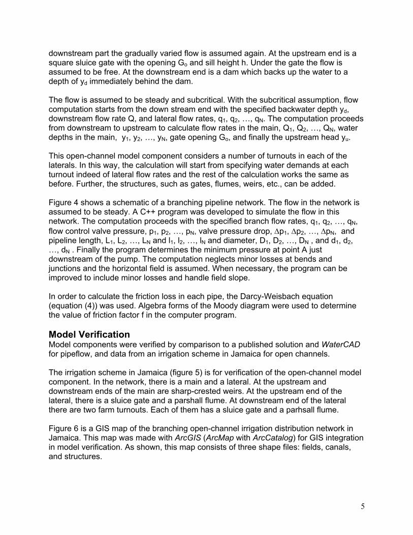
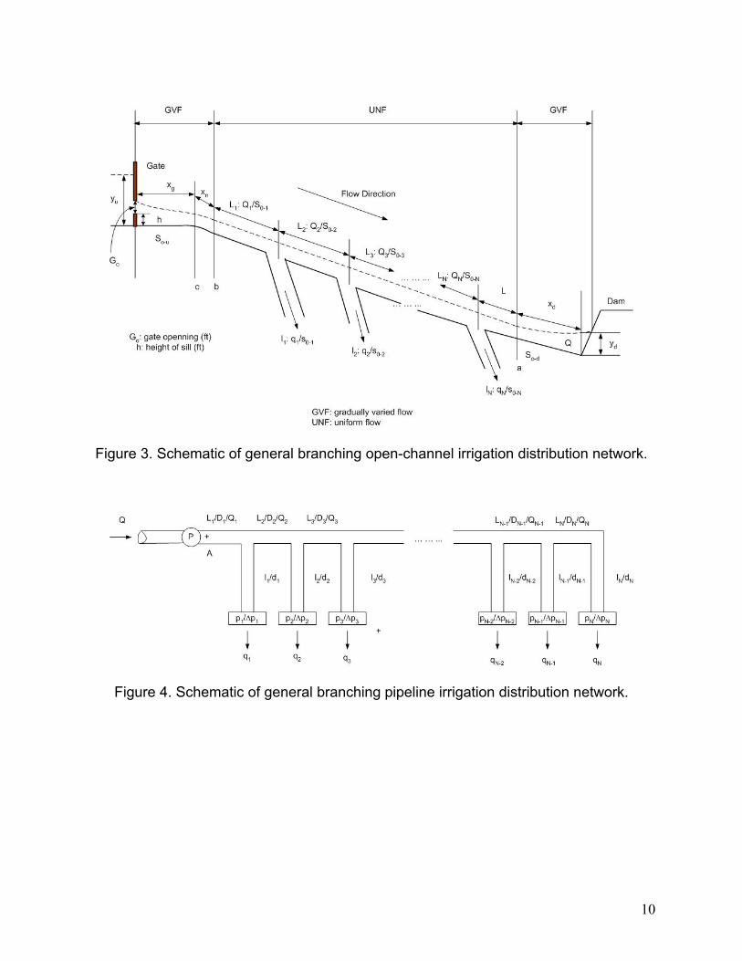
Management Software), a hydraulic model of unsteady flow in branching canal networks (Merkley, 1997); HEC-RAS (Hydraulic Engineering Center –River Analysis System), performing river hydraulic calculations of one-dimensional steady and unsteady flows (Brunner, 2001); and SIC (Simulation of Irrigation Canals), a mathematical model which can simulate the hydraulic behavior of most irrigation canals or rivers, under steady and unsteady flow conditions (Malaterre and Baume, 1997). Software packages are also available for pipe flow analysis. WaterCAD (Haestad et al., 2003) is used for modeling and analysis of pipe distribution networks. The methodology is applicable to any fluid system with the following characteristics: • Steady or gradually-varying turbulent flow • Incompressible, Newtonian, single phase fluids • Full, closed conduits (pressure systems) There have also been FORTRAN programs developed by individual researchers for calculating pipe flow (Jeppson, 1977; Watters, 1979; Watters, 1984; Larock et al., 2000). Materials and Methods In our research, C++ programming language was chosen for the model prototype of open-channel and pipeline distribution networks. The models were designed and developed using the principles of OOP (Object-Oriented Programming). GIS is used for spatial data management, visualization and analysis, and to manage topographical and hydrological data, as well as the model outputs. ArcView is the GIS package used in this research. The integration of GIS data sources can be done in a number of ways. The most straightforward way is to let the models access to GIS data sources directly. In ArcView, attributes describing map features, are stored in dBase tables. C++ model programs can input data from and output results to ArcView directly either by translation between dBase tables and text files or through data source connectivity such as ODBC (Open DataBase Connectivity). Here the integration is realized by translation between dBase tables and text files. In the future data source connectivity will be implemented in order to achieve a higher degree of integration. Figure 2 shows the structure of GIS data connection to the open-channel and pipeline model components. The model accepts data from ArcView and sends results to ArcView by translation between dBase tables and text files. In ArcView values of attributes that describe map features are stored as dBase tables (.dbf files). For data input to the model, original ArcView .dbf files are exported as text (.txt) files that contain values of attributes. Then the model extracts needed data from the text files to perform calculations. Model results are written to text files. ArcView then import these text files by joining original .dbf files to generate new dBase tables. Model Prototype Figure 3 shows a schematic of a branching open-channel network. Flow in this network is divided into three parts: upstream, middle, and downstream. In the upstream part the gradually varied flow is assumed. In the middle part uniform flow is assumed. In the

5

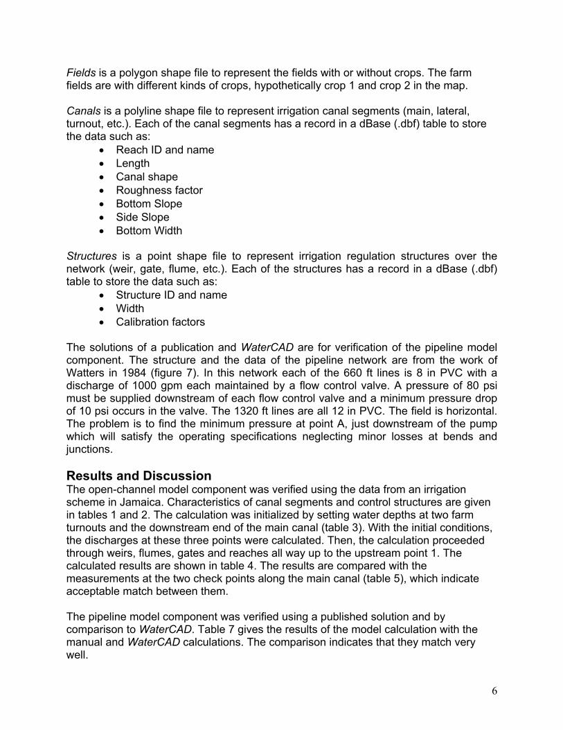
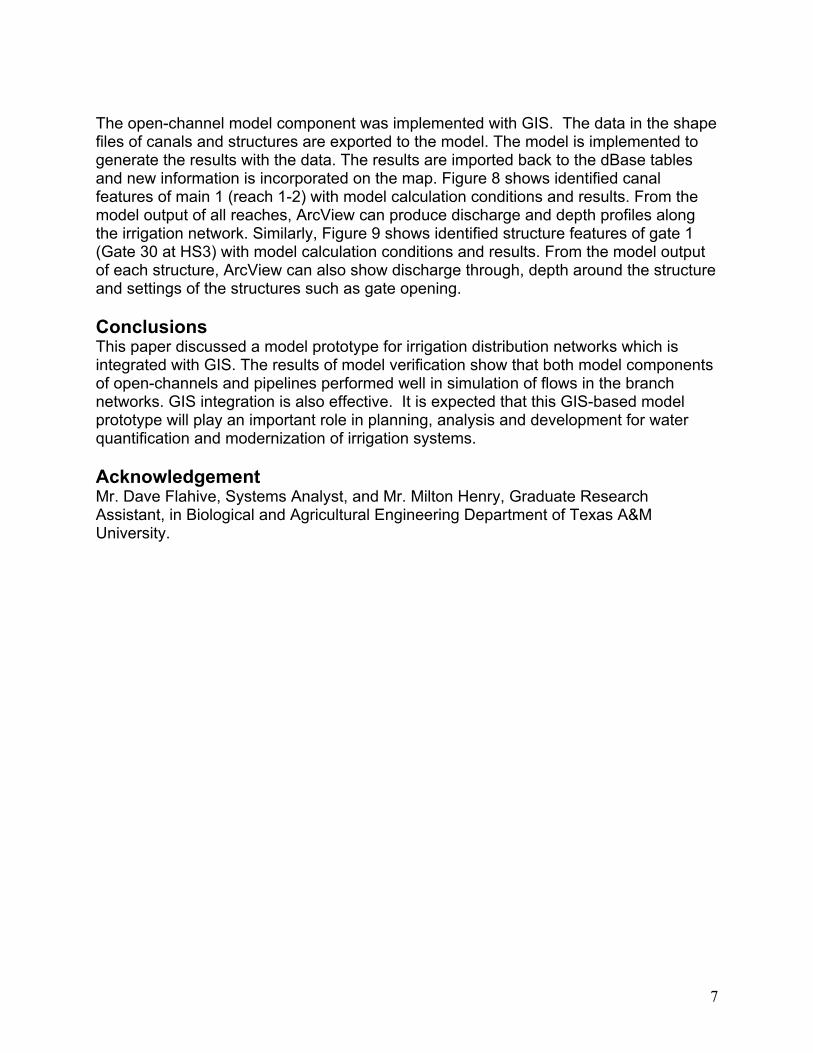
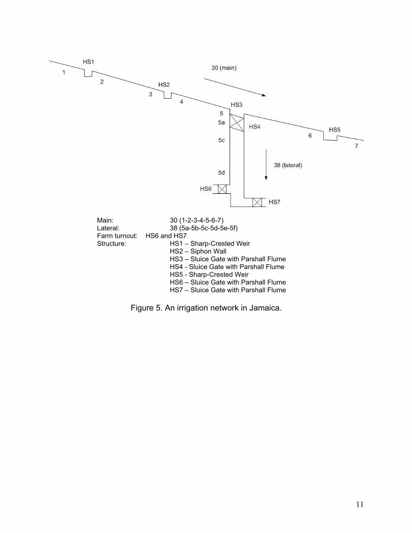
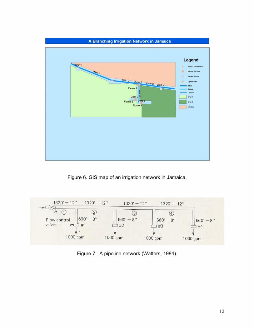
downstream part the gradually varied flow is assumed again. At the upstream end is a square sluice gate with the opening Go and sill height h. Under the gate the flow is assumed to be free. At the downstream end is a dam which backs up the water to a depth of yd immediately behind the dam. The flow is assumed to be steady and subcritical. With the subcritical assumption, flow computation starts from the down stream end with the specified backwater depth yd, downstream flow rate Q, and lateral flow rates, q1, q2, …, qN. The computation proceeds from downstream to upstream to calculate flow rates in the main, Q1, Q2, …, QN, water depths in the main, y1, y2, …, yN, gate opening Go, and finally the upstream head yu. This open-channel model component considers a number of turnouts in each of the laterals. In this way, the calculation will start from specifying water demands at each turnout indeed of lateral flow rates and the rest of the calculation works the same as before. Further, the structures, such as gates, flumes, weirs, etc., can be added. Figure 4 shows a schematic of a branching pipeline network. The flow in the network is assumed to be steady. A C++ program was developed to simulate the flow in this network. The computation proceeds with the specified branch flow rates, q1, q2, …, qN, flow control valve pressure, p1, p2, …, pN, valve pressure drop, ∆p1, ∆p2, …, ∆pN, and pipeline length, L1, L2, …, LN and l1, l2, …, lN and diameter, D1, D2, …, DN , and d1, d2, …, dN . Finally the program determines the minimum pressure at point A just downstream of the pump. The computation neglects minor losses at bends and junctions and the horizontal field is assumed. When necessary, the program can be improved to include minor losses and handle field slope. In order to calculate the friction loss in each pipe, the Darcy-Weisbach equation (equation (4)) was used. Algebra forms of the Moody diagram were used to determine the value of friction factor f in the computer program. Model Verification Model components were verified by comparison to a published solution and WaterCAD for pipeflow, and data from an irrigation scheme in Jamaica for open channels. The irrigation scheme in Jamaica (figure 5) is for verification of the open-channel model component. In the network, there is a main and a lateral. At the upstream and downstream ends of the main are sharp-crested weirs. At the upstream end of the lateral, there is a sluice gate and a parshall flume. At downstream end of the lateral there are two farm turnouts. Each of them has a sluice gate and a parhsall flume. Figure 6 is a GIS map of the branching open-channel irrigation distribution network in Jamaica. This map was made with ArcGIS (ArcMap with ArcCatalog) for GIS integration in model verification. As shown, this map consists of three shape files: fields, canals, and structures.

6

Fields is a polygon shape file to represent the fields with or without crops. The farm fields are with different kinds of crops, hypothetically crop 1 and crop 2 in the map. Canals is a polyline shape file to represent irrigation canal segments (main, lateral, turnout, etc.). Each of the canal segments has a record in a dBase (.dbf) table to store the data such as:

• Reach ID and name • Length • Canal shape • Roughness factor • Bottom Slope • Side Slope • Bottom Width

Structures is a point shape file to represent irrigation regulation structures over the network (weir, gate, flume, etc.). Each of the structures has a record in a dBase (.dbf) table to store the data such as:

• Structure ID and name • Width • Calibration factors

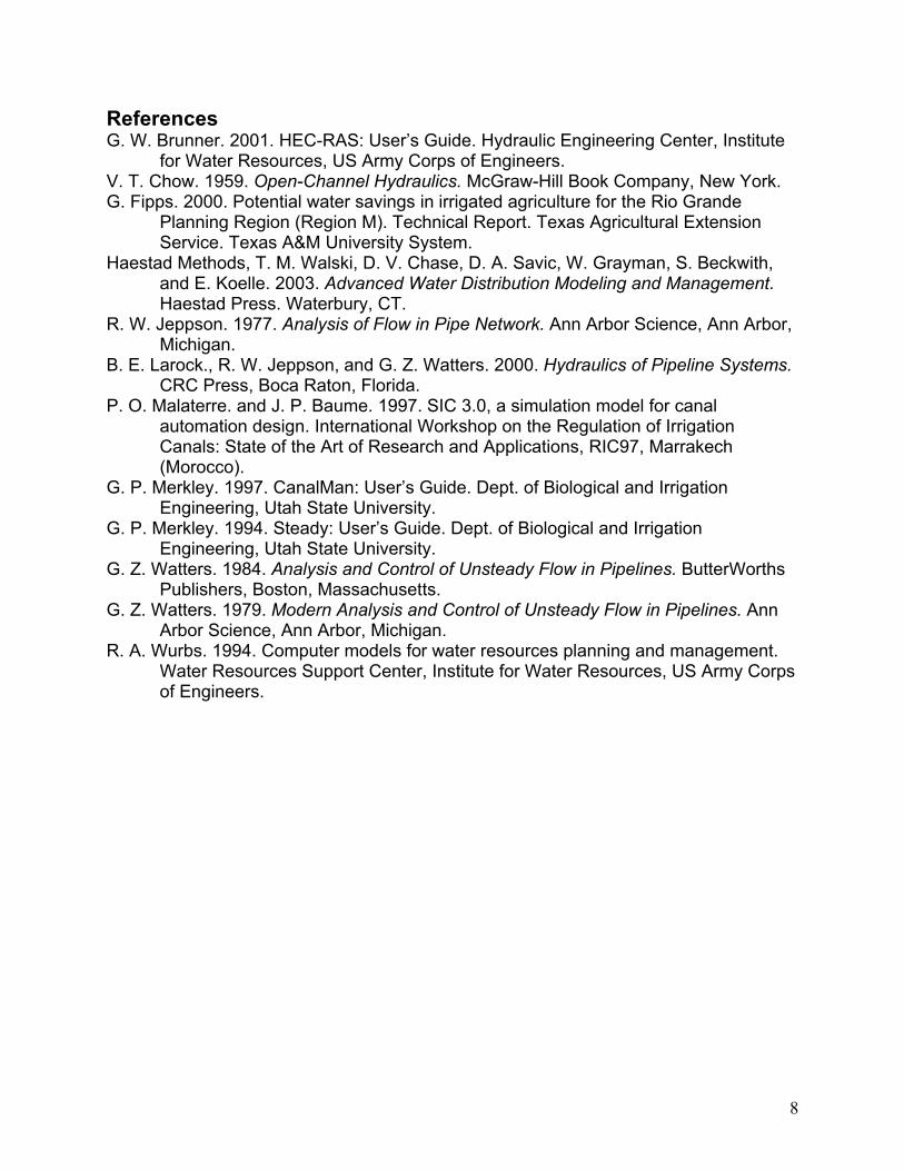
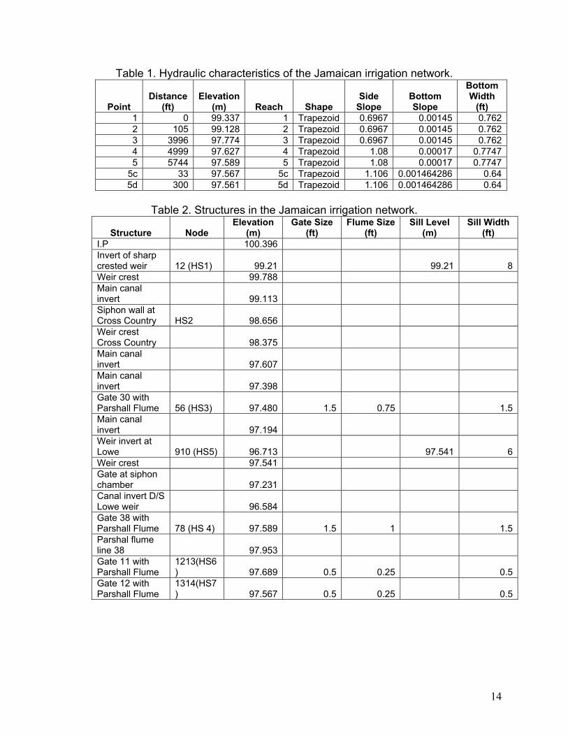
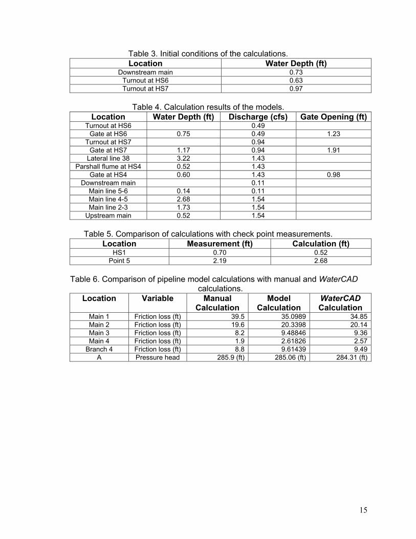
The solutions of a publication and WaterCAD are for verification of the pipeline model component. The structure and the data of the pipeline network are from the work of Watters in 1984 (figure 7). In this network each of the 660 ft lines is 8 in PVC with a discharge of 1000 gpm each maintained by a flow control valve. A pressure of 80 psi must be supplied downstream of each flow control valve and a minimum pressure drop of 10 psi occurs in the valve. The 1320 ft lines are all 12 in PVC. The field is horizontal. The problem is to find the minimum pressure at point A, just downstream of the pump which will satisfy the operating specifications neglecting minor losses at bends and junctions. Results and Discussion The open-channel model component was verified using the data from an irrigation scheme in Jamaica. Characteristics of canal segments and control structures are given in tables 1 and 2. The calculation was initialized by setting water depths at two farm turnouts and the downstream end of the main canal (table 3). With the initial conditions, the discharges at these three points were calculated. Then, the calculation proceeded through weirs, flumes, gates and reaches all way up to the upstream point 1. The calculated results are shown in table 4. The results are compared with the measurements at the two check points along the main canal (table 5), which indicate acceptable match between them. The pipeline model component was verified using a published solution and by comparison to WaterCAD. Table 7 gives the results of the model calculation with the manual and WaterCAD calculations. The comparison indicates that they match very well.

7

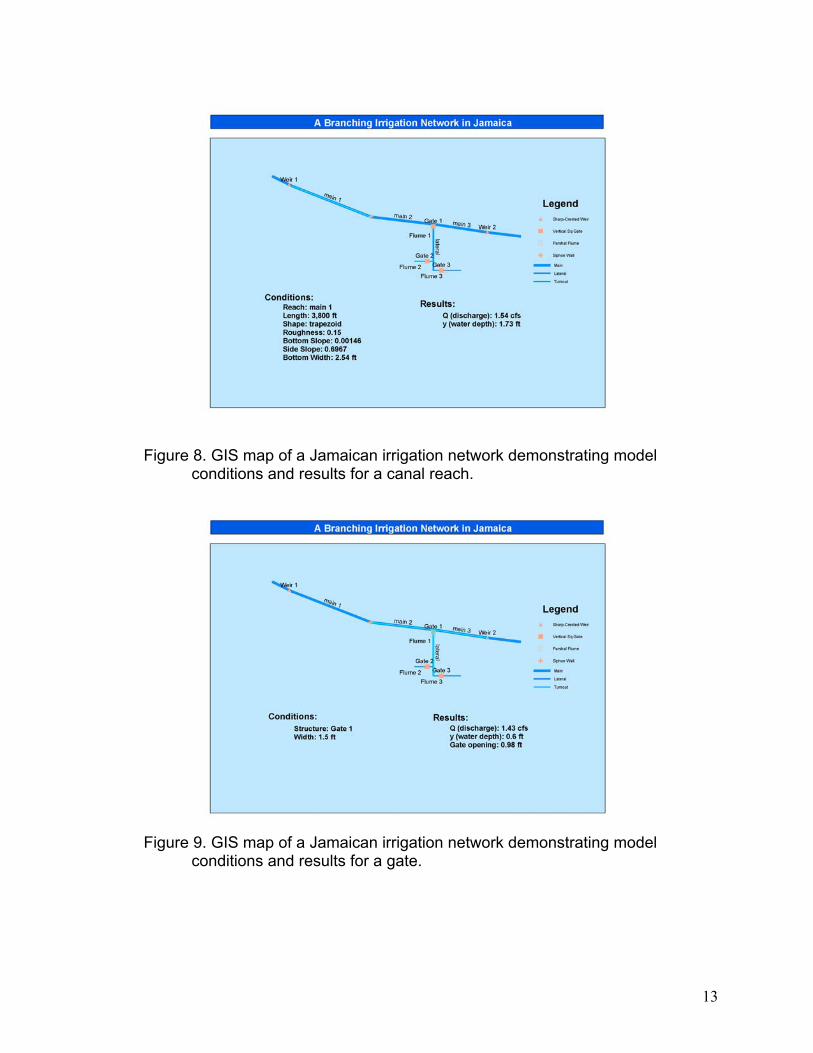
The open-channel model component was implemented with GIS. The data in the shape files of canals and structures are exported to the model. The model is implemented to generate the results with the data. The results are imported back to the dBase tables and new information is incorporated on the map. Figure 8 shows identified canal features of main 1 (reach 1-2) with model calculation conditions and results. From the model output of all reaches, ArcView can produce discharge and depth profiles along the irrigation network. Similarly, Figure 9 shows identified structure features of gate 1 (Gate 30 at HS3) with model calculation conditions and results. From the model output of each structure, ArcView can also show discharge through, depth around the structure and settings of the structures such as gate opening. Conclusions This paper discussed a model prototype for irrigation distribution networks which is integrated with GIS. The results of model verification show that both model components of open-channels and pipelines performed well in simulation of flows in the branch networks. GIS integration is also effective. It is expected that this GIS-based model prototype will play an important role in planning, analysis and development for water quantification and modernization of irrigation systems. Acknowledgement Mr. Dave Flahive, Systems Analyst, and Mr. Milton Henry, Graduate Research Assistant, in Biological and Agricultural Engineering Department of Texas A&M University.

8

References G. W. Brunner. 2001. HEC-RAS: User’s Guide. Hydraulic Engineering Center, Institute

for Water Resources, US Army Corps of Engineers. V. T. Chow. 1959. Open-Channel Hydraulics. McGraw-Hill Book Company, New York. G. Fipps. 2000. Potential water savings in irrigated agriculture for the Rio Grande

Planning Region (Region M). Technical Report. Texas Agricultural Extension Service. Texas A&M University System.

Haestad Methods, T. M. Walski, D. V. Chase, D. A. Savic, W. Grayman, S. Beckwith, and E. Koelle. 2003. Advanced Water Distribution Modeling and Management. Haestad Press. Waterbury, CT.

R. W. Jeppson. 1977. Analysis of Flow in Pipe Network. Ann Arbor Science, Ann Arbor, Michigan.

B. E. Larock., R. W. Jeppson, and G. Z. Watters. 2000. Hydraulics of Pipeline Systems. CRC Press, Boca Raton, Florida.

P. O. Malaterre. and J. P. Baume. 1997. SIC 3.0, a simulation model for canal automation design. International Workshop on the Regulation of Irrigation Canals: State of the Art of Research and Applications, RIC97, Marrakech (Morocco).

G. P. Merkley. 1997. CanalMan: User’s Guide. Dept. of Biological and Irrigation Engineering, Utah State University.

G. P. Merkley. 1994. Steady: User’s Guide. Dept. of Biological and Irrigation Engineering, Utah State University.

G. Z. Watters. 1984. Analysis and Control of Unsteady Flow in Pipelines. ButterWorths Publishers, Boston, Massachusetts.

G. Z. Watters. 1979. Modern Analysis and Control of Unsteady Flow in Pipelines. Ann Arbor Science, Ann Arbor, Michigan.

R. A. Wurbs. 1994. Computer models for water resources planning and management. Water Resources Support Center, Institute for Water Resources, US Army Corps of Engineers.

9

Figure 1. Main irrigation distribution networks in the LRGV.

Figure 2. GIS data input and output with the models.

10

Figure 3. Schematic of general branching open-channel irrigation distribution network.

Figure 4. Schematic of general branching pipeline irrigation distribution network.

11

Main: 30 (1-2-3-4-5-6-7) Lateral: 38 (5a-5b-5c-5d-5e-5f) Farm turnout: HS6 and HS7 Structure: HS1 – Sharp-Crested Weir HS2 – Siphon Wall HS3 – Sluice Gate with Parshall Flume HS4 - Sluice Gate with Parshall Flume HS5 - Sharp-Crested Weir HS6 – Sluice Gate with Parshall Flume HS7 – Sluice Gate with Parshall Flume

Figure 5. An irrigation network in Jamaica.

12

Figure 6. GIS map of an irrigation network in Jamaica.

Figure 7. A pipeline network (Watters, 1984).

13

Figure 8. GIS map of a Jamaican irrigation network demonstrating model conditions and results for a canal reach.

Figure 9. GIS map of a Jamaican irrigation network demonstrating model

conditions and results for a gate.

14

Table 1. Hydraulic characteristics of the Jamaican irrigation network.

Point Distance

(ft) Elevation

(m) Reach Shape Side

Slope Bottom Slope

Bottom Width

(ft) 1 0 99.337 1 Trapezoid 0.6967 0.00145 0.7622 105 99.128 2 Trapezoid 0.6967 0.00145 0.7623 3996 97.774 3 Trapezoid 0.6967 0.00145 0.7624 4999 97.627 4 Trapezoid 1.08 0.00017 0.77475 5744 97.589 5 Trapezoid 1.08 0.00017 0.7747

5c 33 97.567 5c Trapezoid 1.106 0.001464286 0.645d 300 97.561 5d Trapezoid 1.106 0.001464286 0.64

Table 2. Structures in the Jamaican irrigation network.

Structure Node Elevation

(m) Gate Size

(ft) Flume Size

(ft) Sill Level

(m) Sill Width

(ft) I.P 100.396 Invert of sharp crested weir 12 (HS1) 99.21 99.21 8Weir crest 99.788 Main canal invert 99.113 Siphon wall at Cross Country HS2 98.656 Weir crest Cross Country 98.375 Main canal invert 97.607 Main canal invert 97.398 Gate 30 with Parshall Flume 56 (HS3) 97.480 1.5 0.75 1.5Main canal invert 97.194 Weir invert at Lowe 910 (HS5) 96.713 97.541 6Weir crest 97.541 Gate at siphon chamber 97.231 Canal invert D/S Lowe weir 96.584 Gate 38 with Parshall Flume 78 (HS 4) 97.589 1.5 1 1.5Parshal flume line 38 97.953 Gate 11 with Parshall Flume

1213(HS6) 97.689 0.5 0.25 0.5

Gate 12 with Parshall Flume

1314(HS7) 97.567 0.5 0.25 0.5

15

Table 3. Initial conditions of the calculations. Location Water Depth (ft)

Downstream main 0.73 Turnout at HS6 0.63 Turnout at HS7 0.97

Table 4. Calculation results of the models.

Location Water Depth (ft) Discharge (cfs) Gate Opening (ft)Turnout at HS6 0.49

Gate at HS6 0.75 0.49 1.23 Turnout at HS7 0.94

Gate at HS7 1.17 0.94 1.91 Lateral line 38 3.22 1.43

Parshall flume at HS4 0.52 1.43 Gate at HS4 0.60 1.43 0.98

Downstream main 0.11 Main line 5-6 0.14 0.11 Main line 4-5 2.68 1.54 Main line 2-3 1.73 1.54

Upstream main 0.52 1.54

Table 5. Comparison of calculations with check point measurements. Location Measurement (ft) Calculation (ft)

HS1 0.70 0.52 Point 5 2.19 2.68

Table 6. Comparison of pipeline model calculations with manual and WaterCAD

calculations. Location Variable Manual

Calculation Model

Calculation WaterCAD Calculation

Main 1 Friction loss (ft) 39.5 35.0989 34.85Main 2 Friction loss (ft) 19.6 20.3398 20.14Main 3 Friction loss (ft) 8.2 9.48846 9.36Main 4 Friction loss (ft) 1.9 2.61826 2.57

Branch 4 Friction loss (ft) 8.8 9.61439 9.49A Pressure head 285.9 (ft) 285.06 (ft) 284.31 (ft)