Embed Size (px)
Citation preview
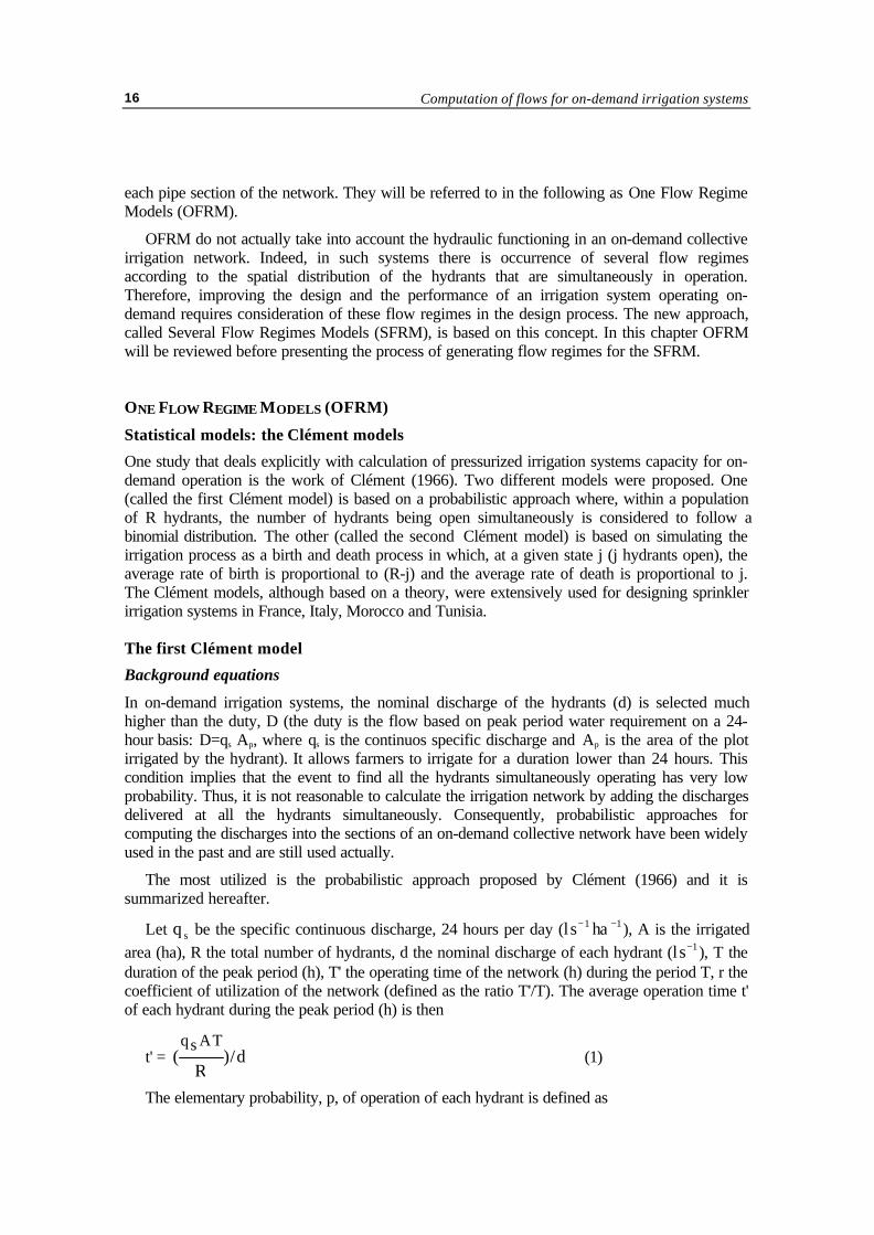
Performance analysis of on-demand pressurized irrigation systems 15
Chapter 3
Computation of flows for on-demandirrigation systems
One of the most important problems for an on-demand irrigation system designer is thecalculation of the discharges flowing into the network. Such discharges strongly vary over timedepending on the cropping pattern, meteorological conditions, on-farm irrigation efficiency andfarmers' behaviour.
In this paper, each group of hydrants operating at a given instant is called “hydrants’configuration”. Each hydrant’s configuration produces a discharge configuration (or flowregime) into the network. The term “node” includes both hydrants and junctions of two pipes,whereas the term “section” is used to describe the pipe connecting any two nodes.
The design capacity is usually determined considering short-term peak demand andconsidering an average cropping pattern for the whole system. But, the individual croppingpattern may differ from the designed one, and the irrigation system may be either undersized oroversized.
In view of the difficulty of this problem, empirical methods have been used. For example, theUS Bureau of Reclamation (1967) recommends solving each case on individual basis and givesonly general indications like: the maximum demand may generally be estimated at 125-150% ofthe average demand. Systems operating for a 12- month season may require a capacity largeenough to carry from 10 to 15% of the total annual demand in the peak month. Those operatingfor a 7-month season may require a capacity large enough to carry from 20 to 25% of the totalannual demand during the peak month. However, the actual maximum demand should bedetermined by detailed analysis of individual projects.
The advent of on-demand, large-scale irrigation systems in the early 1960s in France fosteredthe development of statistical models to compute the design flows. Examples of such models arethe first and the second Clément formula (1966). But only the first demand formula has beenwidely used because of its simplicity.
Although these models are theoretically sound, the assumptions governing the determinationof their parameters do not take into account the actual functioning of an irrigation system. Inview of these limitations a number of researchers tackled the problem by simulating irrigationstrategies. As an example, Maidment and Hutchinson (1983) modeled the demand pattern over alarge irrigation area taking into account the size of irrigated area, the soil type, the croppingpattern, the irrigation strategy and the weather variation. However, they had to average out thedemand hydrograph over time to avoid unrealistic very high water demand one day and very lowthe next.
Recently other approaches have been developed combining simulation of irrigation strategies,based on the soil water balance, and statistical models (Abdellaoui, 1986; Walker et al., 1995;Teixeira et al., 1995). The result of these methods is a single distribution of one design flow for
Computation of flows for on-demand irrigation systems16
each pipe section of the network. They will be referred to in the following as One Flow RegimeModels (OFRM).
OFRM do not actually take into account the hydraulic functioning in an on-demand collectiveirrigation network. Indeed, in such systems there is occurrence of several flow regimesaccording to the spatial distribution of the hydrants that are simultaneously in operation.Therefore, improving the design and the performance of an irrigation system operating on-demand requires consideration of these flow regimes in the design process. The new approach,called Several Flow Regimes Models (SFRM), is based on this concept. In this chapter OFRMwill be reviewed before presenting the process of generating flow regimes for the SFRM.
ONE FLOW REGIME MODELS (OFRM)
Statistical models: the Clément models
One study that deals explicitly with calculation of pressurized irrigation systems capacity for on-demand operation is the work of Clément (1966). Two different models were proposed. One(called the first Clément model) is based on a probabilistic approach where, within a populationof R hydrants, the number of hydrants being open simultaneously is considered to follow abinomial distribution. The other (called the second Clément model) is based on simulating theirrigation process as a birth and death process in which, at a given state j (j hydrants open), theaverage rate of birth is proportional to (R-j) and the average rate of death is proportional to j.The Clément models, although based on a theory, were extensively used for designing sprinklerirrigation systems in France, Italy, Morocco and Tunisia.
The first Clément model
Background equations
In on-demand irrigation systems, the nominal discharge of the hydrants (d) is selected muchhigher than the duty, D (the duty is the flow based on peak period water requirement on a 24-hour basis: D=qs Ap, where qs is the continuos specific discharge and Ap is the area of the plotirrigated by the hydrant). It allows farmers to irrigate for a duration lower than 24 hours. Thiscondition implies that the event to find all the hydrants simultaneously operating has very lowprobability. Thus, it is not reasonable to calculate the irrigation network by adding the dischargesdelivered at all the hydrants simultaneously. Consequently, probabilistic approaches forcomputing the discharges into the sections of an on-demand collective network have been widelyused in the past and are still used actually.
The most utilized is the probabilistic approach proposed by Clément (1966) and it issummarized hereafter.
Let q s be the specific continuous discharge, 24 hours per day (l s ha1 1− − ), A is the irrigatedarea (ha), R the total number of hydrants, d the nominal discharge of each hydrant (l s 1− ), T theduration of the peak period (h), T' the operating time of the network (h) during the period T, r thecoefficient of utilization of the network (defined as the ratio T'/T). The average operation time t'of each hydrant during the peak period (h) is then
t' = d/)R
(TAsq
(1)
The elementary probability, p, of operation of each hydrant is defined as
Performance analysis of on-demand pressurized irrigation systems 17
p = Tr
1
dR
TAsq
Tr
t'
T'
t'== (2)
thus,
p =q A
r R ds (3)
Therefore, for a population of R homogeneous hydrants, the probability of finding one hydrantopen is p, while (1 - p) is the probability to find it closed.
The number of operating hydrants is considered a random variable having a binomialdistribution with mean
µ = R p (4)
and variance
σ2 = R p (1-p) (5)
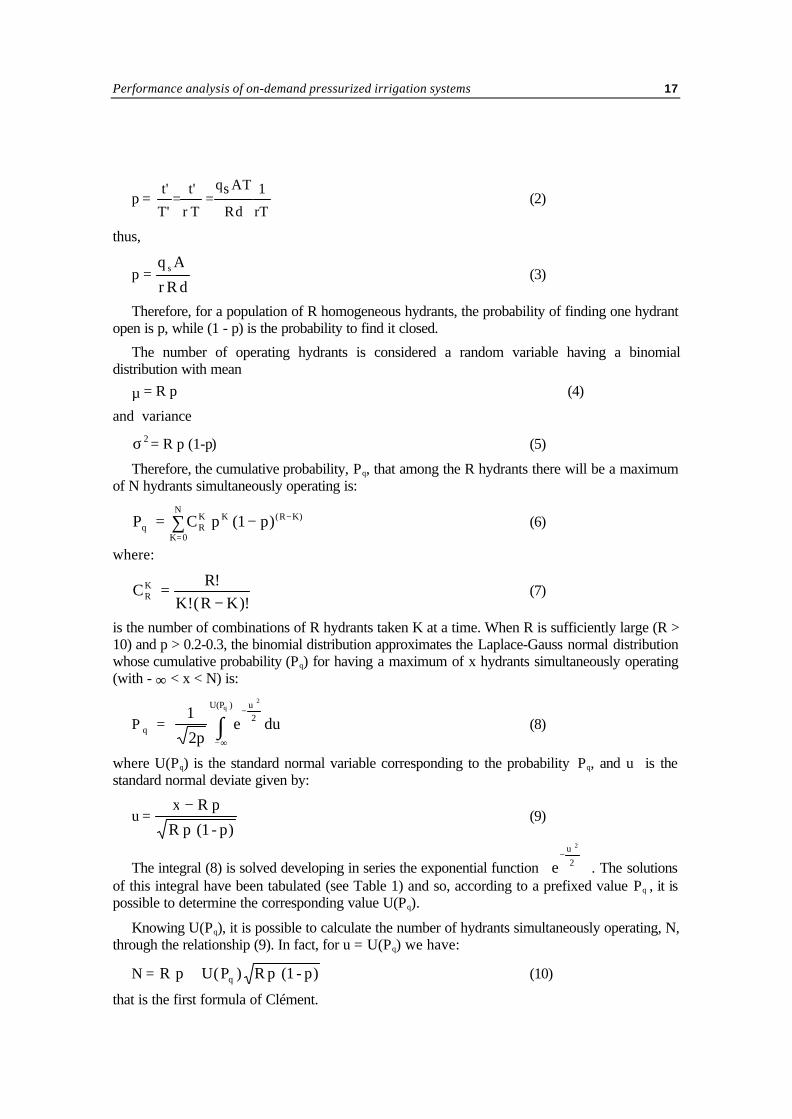
Therefore, the cumulative probability, Pq, that among the R hydrants there will be a maximumof N hydrants simultaneously operating is:
P C pq RK
K 0
NK (R K)= −
=
−∑ ( )1 p (6)
where:
CR!
K!(R K)!RK =
− (7)
is the number of combinations of R hydrants taken K at a time. When R is sufficiently large (R >10) and p > 0.2-0.3, the binomial distribution approximates the Laplace-Gauss normal distributionwhose cumulative probability (Pq) for having a maximum of x hydrants simultaneously operating(with - ∞ < x < N) is:
P q = due2p
1 2u )U(P 2
q −
∞−∫ (8)
where U(Pq) is the standard normal variable corresponding to the probability Pq, and u is thestandard normal deviate given by:
u = x R p
R p (1 - p)
− (9)
The integral (8) is solved developing in series the exponential function eu 2
2−
. The solutionsof this integral have been tabulated (see Table 1) and so, according to a prefixed value Pq , it ispossible to determine the corresponding value U(Pq).
Knowing U(Pq), it is possible to calculate the number of hydrants simultaneously operating, N,through the relationship (9). In fact, for u = U(Pq) we have:
N = R p U(P ) R p (1 - p)q+ (10)
that is the first formula of Clément.
Computation of flows for on-demand irrigation systems18
Considering hydrants with the same discharge, the totaldischarge downstream a generic section k is given by:
Q = R p d U(P ) R p dk q2+ −( )1 p (11)
and, for different discharges of hydrants (di,), where I is thehydrant class number
Q = R p d U(P ) R p dk i i i i q i i i i i2∑ ∑+ −( )1 p (12)
The first Clément model is based on three major hypothesesthat limit its applicability (CTGREF, 1974; CTGREF, 1977;Lamaddalena and Ciollaro, 1993).
• The first hypothesis concerns the parameter r. It is defined byClément as coefficient of utilization of the system in the sensethat, during the design phase, the duration of the day for irrigation, within the peak period, isconsidered shorter than 24 hours. This parameter, defined at the network level in an irrigationsystem operating on-demand, should have a value equal to one because these systems mayhave to work 24 hours per day. In practice, the parameter r should correspond to theoperating time of each hydrant and, therefore, it is not correct to use it for the global design ofthe system. Nevertheless, from a conceptual point of view, it may be considered as aparameter which helps adjusting the theoretical formulation to a homogeneous population ofdischarges, withdrawn in the field, appropriately chosen through a statistical approach. It mustbe pointed out that the Clément model, like all other models, only offers a schematicrepresentation of an actual network. Therefore, it must be adjusted or calibrated byintroducing field data relative to existing networks. In particular, values of the parameter rshould be, whenever possible, selected for homogeneous regions and for particular crops. Anexample of the field Clément model calibration, for an Italian irrigation network, is reported inAnnex 1.
• The second hypothesis concerns the elementary probability of opening each hydrant. It refersto an estimation of the average operating time of each hydrant. But, the probability to find ahydrant working at a given time t depends on its state at the previous time t-1. In order tojustify the binomial law, this probability should characterize a series of events such that whenthe farmer opens his hydrant at a time t, he would close it after a laps of time dt, and hedecides to re-open or to leave it closed at a successive time t+dt, and so on. This is not realbecause a farmer opens his hydrant and leaves it in the same state for a large number of lapsof time dt. Moreover, the elementary probability varies during the day according to thefarmer's behaviour.
• The third hypothesis considers the independence of the hydrants and their random operationduring the peak period. This hypothesis might seem justified because the farmers shouldbehave autonomously and not according to the operation of the neighbour farmers.Nevertheless, the rhythm of nights and days and the similitude of the crops within an irrigationdistrict condition the farmer's behaviour, so that this hypothesis is not fully reliable.The importance of the r coefficient is stressed also in Figure 10. In this figure two parameters
are defined: the elasticity of the network, eR (Clément and Galand, 1979):
e R = A q
Q
s
Cl (13)
and the average elasticity of the hydrants (called also farmers “degree of freedom”), e h,
TABLE 1Standard normal cumulativedistribution function
Pq U(Pq)0.90 1.2850.91 1.3450.92 1.4050.93 1.4750.94 1.5550.95 1.6450.96 1.7550.97 1.8850.98 2.0550.99 2.324
Performance analysis of on-demand pressurized irrigation systems 19
e h =R d
(q A)s
(14)
The ratio e R is a measure of the over-capacity of the network and is a characteristic of on-demand operation. The ratio e h defines the freedom afforded to farmers to organize theirirrigation.
The values of eR refer to a network designed to supply equal flows at all hydrants. When thehydrant design flows are unequal, the values of the ratio are slightly greater. Nevertheless,whether the hydrants are homogeneous or not, taking into account the probability of the demandbeing spread results in a network peak design flow which is very much smaller than that whichwould be obtained by summating the flows at all hydrants.
The degree of freedom that is to be afforded to farmers should be selected according tocriteria such as size and dispersion of plots, availability of labor, type of on-farm equipment,frequency of irrigation. Hydrants with capacities of one and a half to twice the value of the dutycorrespond to the lowest feasible degree of freedom. With smaller values, the probability of anhydrant being open becomes too great for the demand model to apply. Conversely, hydrantcapacities should not exceed six to eight times the value of the duty. This corresponds to a veryhigh degree of freedom.
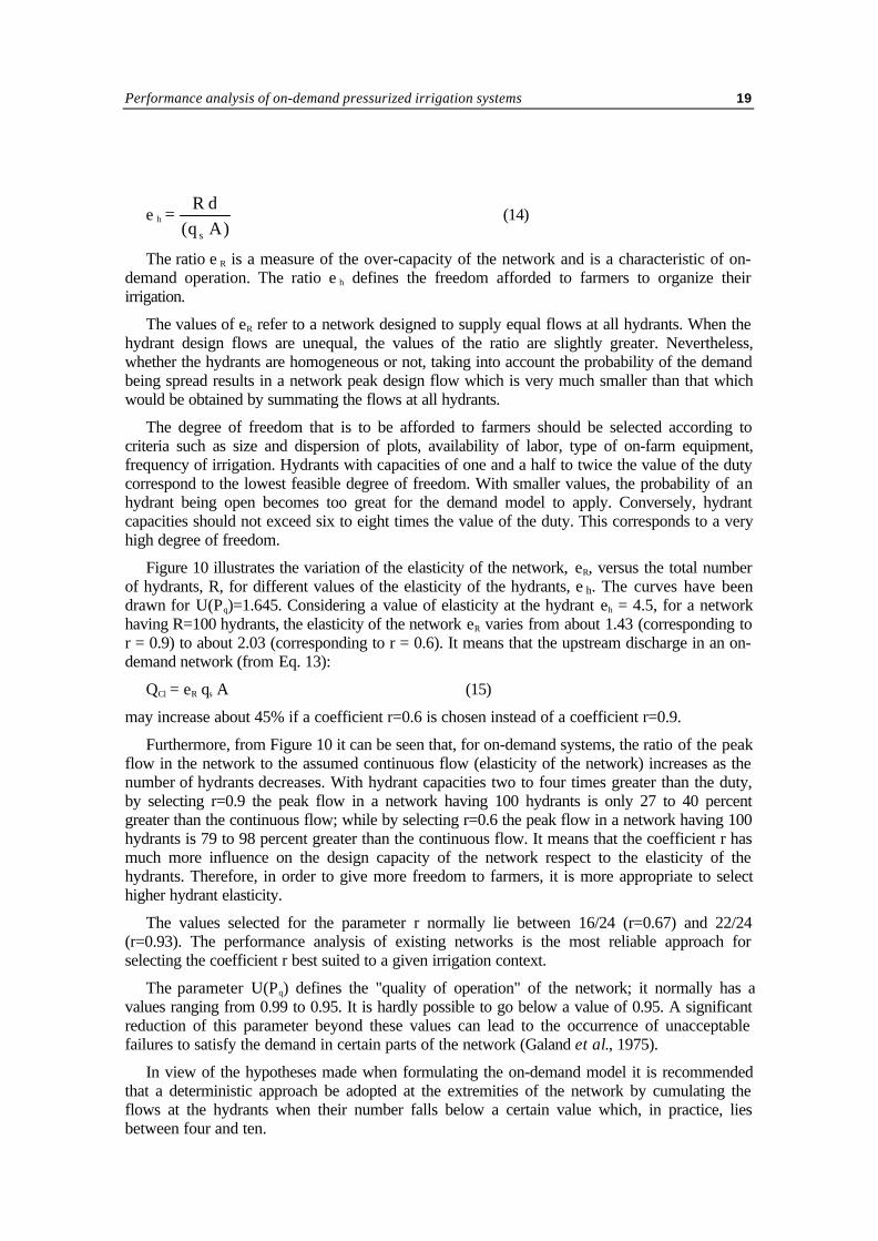
Figure 10 illustrates the variation of the elasticity of the network, eR, versus the total numberof hydrants, R, for different values of the elasticity of the hydrants, e h. The curves have beendrawn for U(Pq)=1.645. Considering a value of elasticity at the hydrant eh = 4.5, for a networkhaving R=100 hydrants, the elasticity of the network eR varies from about 1.43 (corresponding tor = 0.9) to about 2.03 (corresponding to r = 0.6). It means that the upstream discharge in an on-demand network (from Eq. 13):
QCl = eR qs A (15)
may increase about 45% if a coefficient r=0.6 is chosen instead of a coefficient r=0.9.
Furthermore, from Figure 10 it can be seen that, for on-demand systems, the ratio of the peakflow in the network to the assumed continuous flow (elasticity of the network) increases as thenumber of hydrants decreases. With hydrant capacities two to four times greater than the duty,by selecting r=0.9 the peak flow in a network having 100 hydrants is only 27 to 40 percentgreater than the continuous flow; while by selecting r=0.6 the peak flow in a network having 100hydrants is 79 to 98 percent greater than the continuous flow. It means that the coefficient r hasmuch more influence on the design capacity of the network respect to the elasticity of thehydrants. Therefore, in order to give more freedom to farmers, it is more appropriate to selecthigher hydrant elasticity.
The values selected for the parameter r normally lie between 16/24 (r=0.67) and 22/24(r=0.93). The performance analysis of existing networks is the most reliable approach forselecting the coefficient r best suited to a given irrigation context.
The parameter U(Pq) defines the "quality of operation" of the network; it normally has avalues ranging from 0.99 to 0.95. It is hardly possible to go below a value of 0.95. A significantreduction of this parameter beyond these values can lead to the occurrence of unacceptablefailures to satisfy the demand in certain parts of the network (Galand et al., 1975).
In view of the hypotheses made when formulating the on-demand model it is recommendedthat a deterministic approach be adopted at the extremities of the network by cumulating theflows at the hydrants when their number falls below a certain value which, in practice, liesbetween four and ten.
Computation of flows for on-demand irrigation systems20
In certain cases it may happen that the calculated discharge of a section serving five or sixhydrants is less than that of the downstream section serving four hydrants whose flows havebeen summed. In this case the discharge in the upstream section will be equal the discharge inthe downstream section.
Determination of the specific continuous discharge
In order to apply the above methodology it is necessary to know the value of the specificcontinuous discharge, qs (l s-1 ha-1) in the network downstream of the section under consideration.Its value can readily be determined when:
• The cropping pattern is identical throughout the area. If this is so the specific continuousdischarge, qs (l s-1 ha-1), estimated by giving due weight to each of the crops, holds good forevery farm and all branches of the network under consideration.
• The cropping intensity is identical throughout the area. When this is so, the ratio between thenet irrigated area and the gross area also holds good for every holding and all parts of thenetwork under study.
A number of computer packages are available for such a computation (CROPWAT,ISAREG, etc.), as well as an extensive literature. Therefore, the reader is referred to them forits calculation.
Discharge at the hydrants
Although a farmer supplied by an on-demand system is free to use his hydrant at any time, aphysical constraint is nevertheless imposed as regards the maximum flow he can draw. This isachieved by fitting the hydrant with a flow regulator (flow limiter). The discharge attributed toeach hydrant is defined according to the size and crop water requirements of the plot. It is
FIGURE 10Variation of the elasticity of the network, eR, versus the total number of hydrants for differentvalues of r and eh, for U(Pq) = 1.645.
Performance analysis of on-demand pressurized irrigation systems 21
always greater than the duty so as to give the farmer a certain degree of freedom in themanagement of the irrigation.
The ratio between the discharge attributed to each hydrant and the duty is a measure of the"degree of freedom" which a farmer has to manage irrigation. The wide variety of agronomicsituations is reflected by the wide range of the value of the degree of freedom found in practice(FAO-44, 1990):
• High degree of freedom: family holdings with limited labour, low crop water requirements,small or scattered plots, low investment level in on-farm equipment;
• Low degree of freedom: large size plots, large scale farming, abundant labour, highinvestment level in on-farm equipment.
Since the maximum flow at hydrants is fixed by flow regulators it is usual to opt for astandard range of flows. Such ranges vary from country to country.
In southeastern France, for instance, a range of six hydrants has been standardized,corresponding to the following discharges:
Class of hydrant 0 1 2 3 4 5Discharge (l s
-1) 2.1 4.2 8.3 13.9 20.8 27.8
In Italy the range of hydrants corresponds to the following discharges:
Class of hydrant 0 1 2 3 4 5Discharge (l s
-1) 2.5 5 10 15 20 25
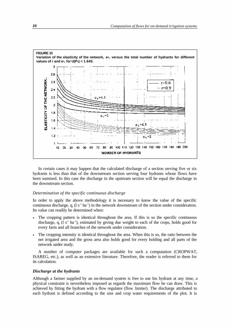
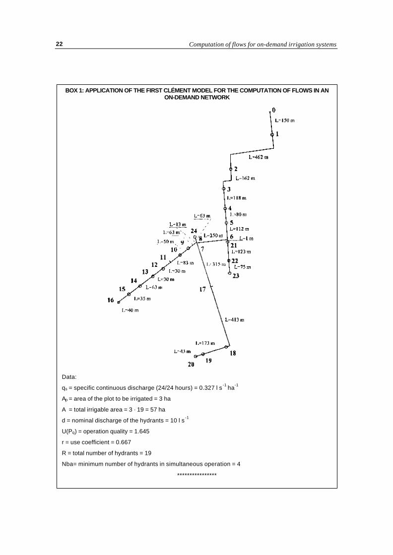
In Box 1, an example of the Clément formula is worked out and the results are shown inTable 2 (generated by COPAM).
TABLE 2Discharges flowing into each section of the network under study (output of the COPAM package:computation with the first Clément model)
Section Initial Final Number of Area 1st ClémentNumber Node Node Hydrants (ha) discharge (l/s)******************************************************** 1 0 1 19 57.00 60.00 2 1 2 18 54.00 60.00 3 2 3 17 51.00 50.00 4 3 4 16 48.00 50.00 5 4 5 15 45.00 50.00 6 5 6 14 42.00 50.00 7 6 7 11 33.00 40.00 8 7 8 8 24.00 40.00 9 8 9 7 21.00 40.00 10 9 10 6 18.00 40.00 11 10 11 5 15.00 40.00 12 11 12 5 15.00 40.00 13 12 13 4 12.00 40.00 14 13 14 3 9.00 30.00 15 14 15 2 6.00 20.00 16 15 16 1 3.00 10.00 17 7 17 3 9.00 30.00 18 17 18 3 9.00 30.00 19 18 19 2 6.00 20.00 20 19 20 1 3.00 10.00 21 6 21 3 9.00 30.00 22 21 22 2 6.00 20.00 23 22 23 1 3.00 10.00 24 8 24 1 3.00 10.00
Computation of flows for on-demand irrigation systems22
L=43 m
L=173 m
L=413 m
BOX 1: APPLICATION OF THE FIRST CLÉMENT MODEL FOR THE COMPUTATION OF FLOWS IN ANON-DEMAND NETWORK
Data:
qs = specific continuous discharge (24/24 hours) = 0.327 l s -1 ha-1
Ap = area of the plot to be irrigated = 3 ha
A = total irrigable area = 3 · 19 = 57 ha
d = nominal discharge of the hydrants = 10 l s -1
U(Pq) = operation quality = 1.645
r = use coefficient = 0.667
R = total number of hydrants = 19
Nba= minimum number of hydrants in simultaneous operation = 4
****************
Performance analysis of on-demand pressurized irrigation systems 23
In order to facilitate the calculation of large networks, a computer software program calledCOPAM (Combined Optimization and Performance Analysis Model) has been developed byLamaddalena (1997). This software (enclosed) has several options that will be explained in thispaper.
All the computer programs for computation of irrigation systems require detailed informationon the pipe network transporting water from the source to the demand points (hydrants). In thefollowing section some general information on the use of COPAM, as well as the installation ofthe program and the preparation of the input data files, are presented.
Installation of COPAM
Basic Windows knowledge is required for installing the COPAM Package.
Create an appropriate directory in the hard disk (it can be called “Copam”),
Insert the install disk in the appropriate drive,
Copy all files from the install disk to the directory previously created (e.g. Copam). Verify thatthe “*.dll” files have been copied,
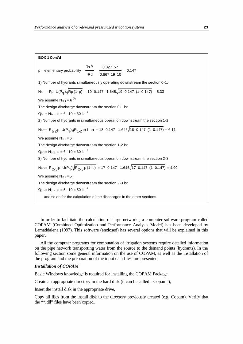
BOX 1 Cont’d
p = elementary probability =dRr
Asq=
10 19 0.667
57 0.327
⋅⋅
⋅= 0.147
1) Number of hydrants simultaneously operating downstream the section 0-1:
N0-1 = p)-(1 pR)qU(PpR + = 0.147)-(1 0.147 191.645 0.147 19 ⋅⋅+⋅ = 5.33
We assume N 0-1 = 6 (1)
The design discharge downstream the section 0-1 is:
Q0-1 = N0-1 · d = 6 · 10 = 60 l s -1
2) Number of hydrants in simultaneous operation downstream the section 1-2:
N1-2 = p)-(1 p2-1R)qU(Pp2-1R + = 0.147)-(1 0.147 181.645 0.147 18 ⋅⋅+⋅ = 6.11
We assume N 1-2 = 6
The design discharge downstream the section 1-2 is:
Q1-2 = N1-2 · d = 6 · 10 = 60 l s -1
3) Number of hydrants in simultaneous operation downstream the section 2-3:
N2-3 = p)-(1 p3-2R)qU(Pp3-2R + = 0.147)-(1 0.147 171.645 0.147 17 ⋅⋅+⋅ = 4.90
We assume N 2-3 = 5
The design discharge downstream the section 2-3 is:
Q2-3 = N2-3 · d = 5 · 10 = 50 l s -1
and so on for the calculation of the discharges in the other sections.
Computation of flows for on-demand irrigation systems24
From Windows Explorer, open the directory Copam and create ashortcut on the desktop for the file (icon) “copam.exe”,
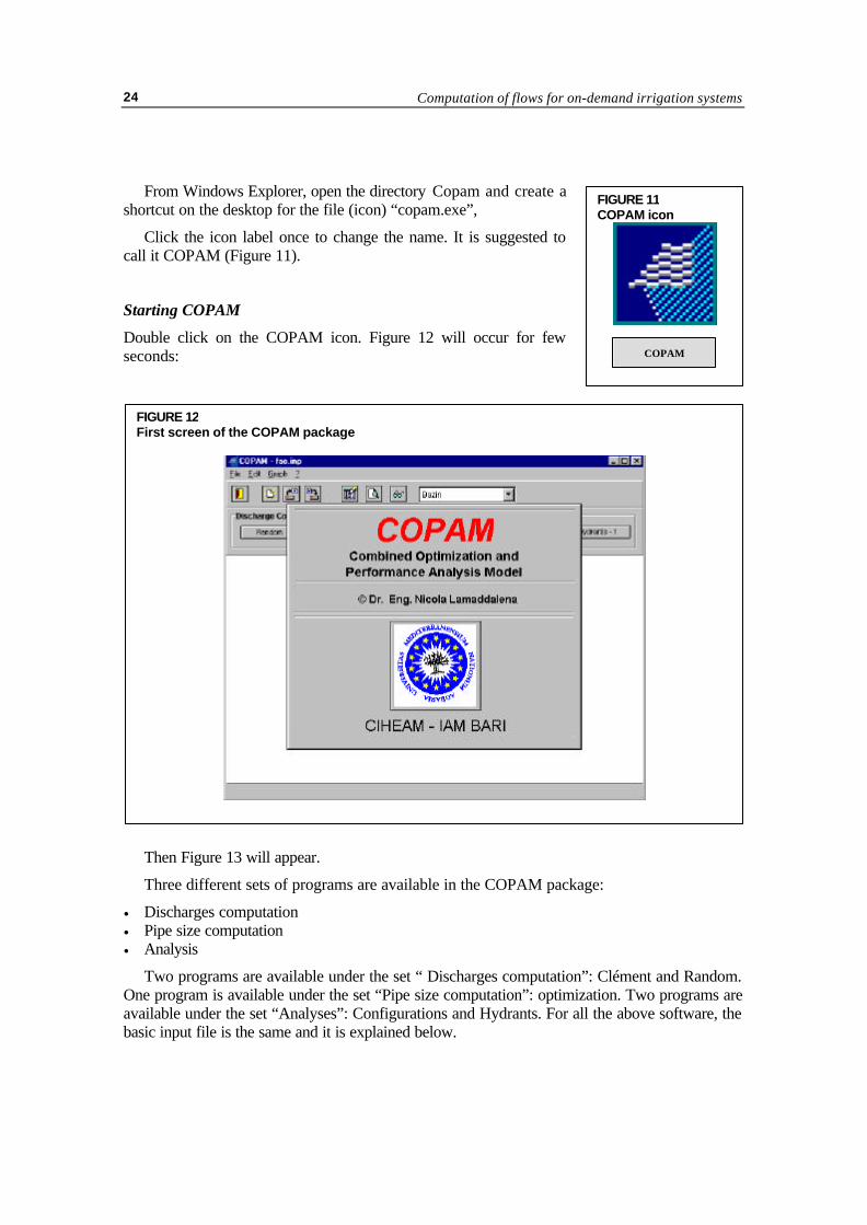
Click the icon label once to change the name. It is suggested tocall it COPAM (Figure 11).
Starting COPAM
Double click on the COPAM icon. Figure 12 will occur for fewseconds:
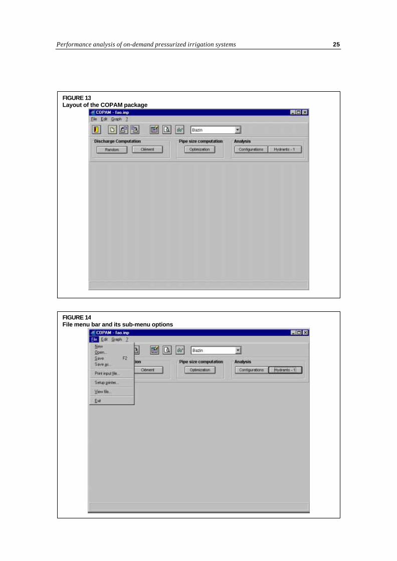
Then Figure 13 will appear.
Three different sets of programs are available in the COPAM package:
• Discharges computation• Pipe size computation• Analysis
Two programs are available under the set “ Discharges computation”: Clément and Random.One program is available under the set “Pipe size computation”: optimization. Two programs areavailable under the set “Analyses”: Configurations and Hydrants. For all the above software, thebasic input file is the same and it is explained below.
FIGURE 11COPAM icon
COPAM
FIGURE 12First screen of the COPAM package
Performance analysis of on-demand pressurized irrigation systems 25
FIGURE 13Layout of the COPAM package
FIGURE 14File menu bar and its sub-menu options
Computation of flows for on-demand irrigation systems26
Preparation of the input file
The line of words beginning “File” is a menu bar. When you click on any of the words with yourmouse, a sub-menu will drop down. For example, if you click on the File menu, you will see thesub-menu in Figure 14.
Different options are available in the File menu: New, Open, Save, Save as, Print input file,Setup printer, View file, Exit. All these options are familiar for windows users.
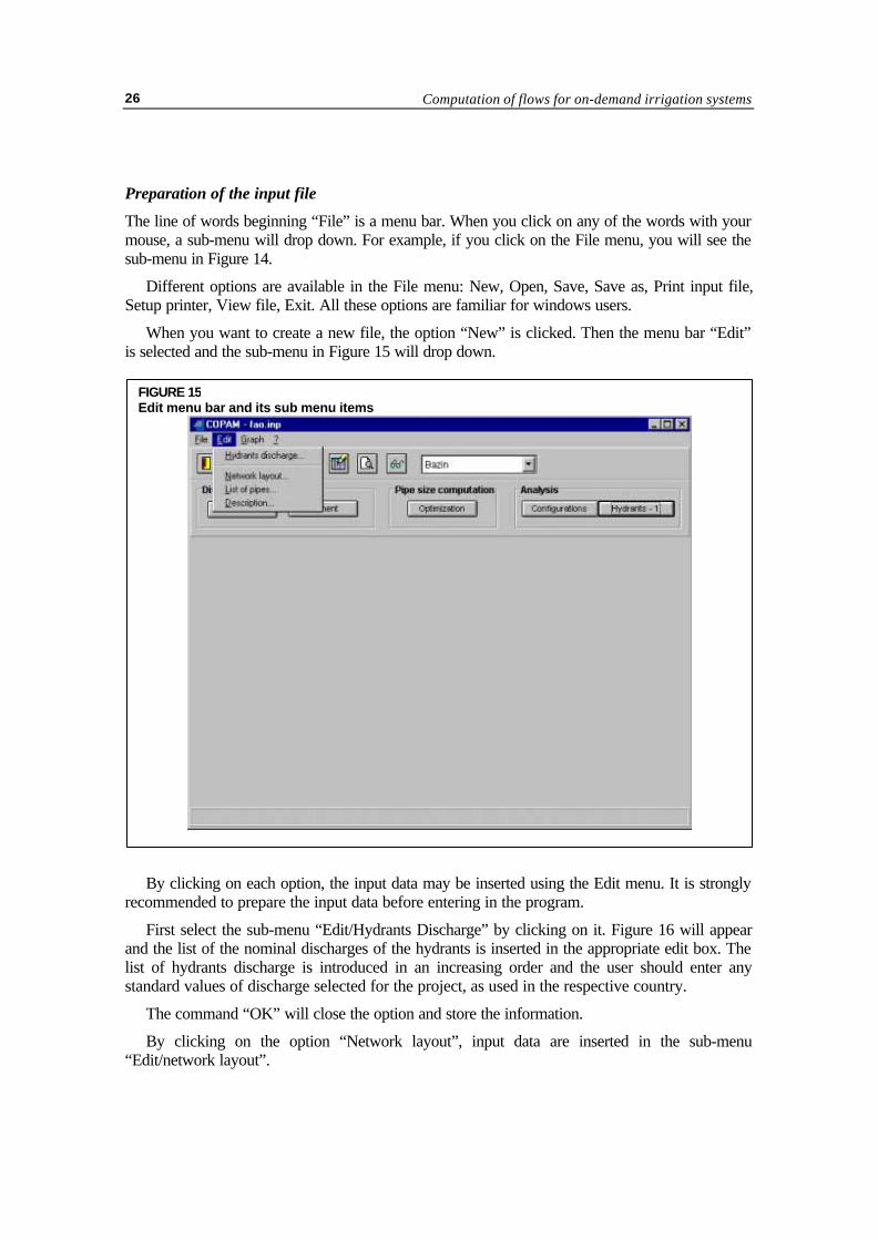
When you want to create a new file, the option “New” is clicked. Then the menu bar “Edit”is selected and the sub-menu in Figure 15 will drop down.
By clicking on each option, the input data may be inserted using the Edit menu. It is stronglyrecommended to prepare the input data before entering in the program.
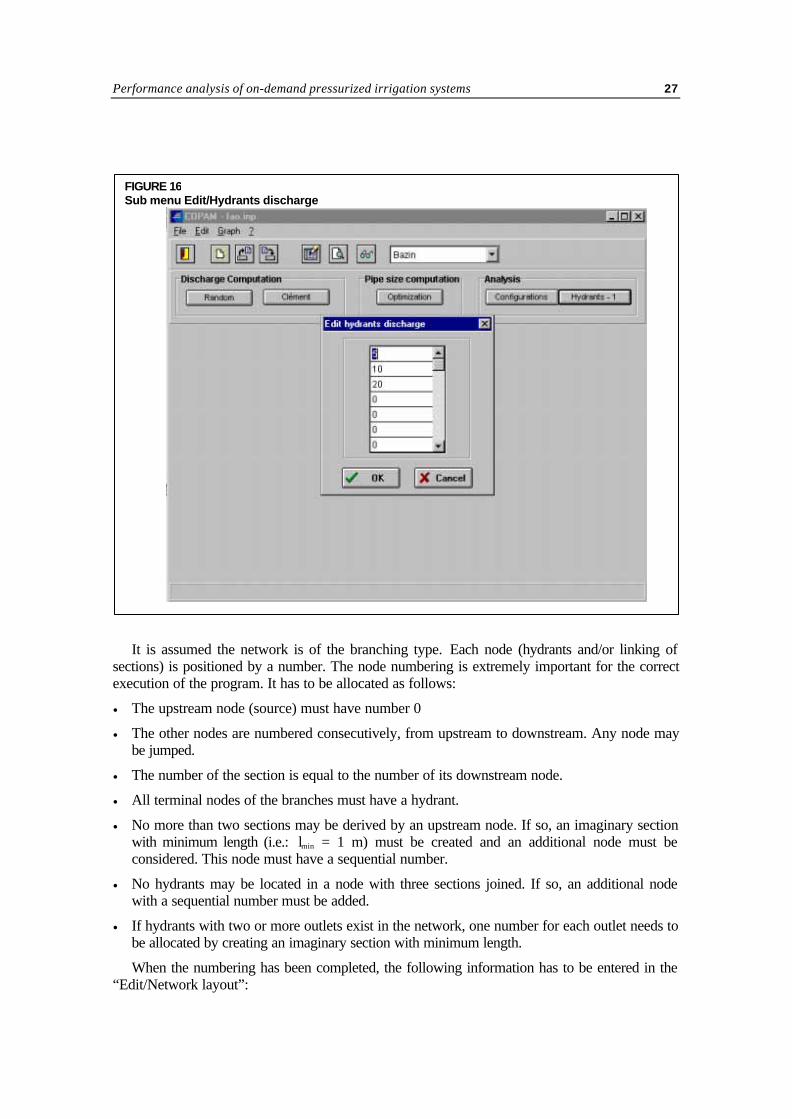
First select the sub-menu “Edit/Hydrants Discharge” by clicking on it. Figure 16 will appearand the list of the nominal discharges of the hydrants is inserted in the appropriate edit box. Thelist of hydrants discharge is introduced in an increasing order and the user should enter anystandard values of discharge selected for the project, as used in the respective country.
The command “OK” will close the option and store the information.
By clicking on the option “Network layout”, input data are inserted in the sub-menu“Edit/network layout”.
FIGURE 15Edit menu bar and its sub menu items
Performance analysis of on-demand pressurized irrigation systems 27
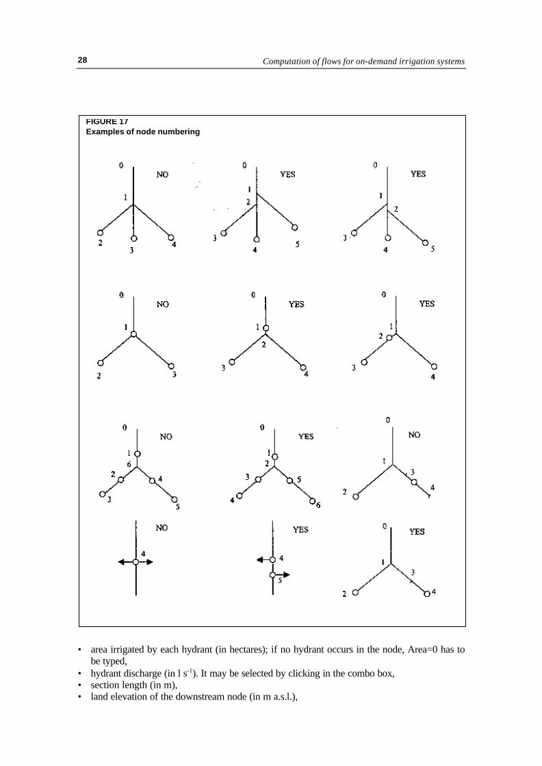
It is assumed the network is of the branching type. Each node (hydrants and/or linking ofsections) is positioned by a number. The node numbering is extremely important for the correctexecution of the program. It has to be allocated as follows:
• The upstream node (source) must have number 0
• The other nodes are numbered consecutively, from upstream to downstream. Any node maybe jumped.
• The number of the section is equal to the number of its downstream node.
• All terminal nodes of the branches must have a hydrant.
• No more than two sections may be derived by an upstream node. If so, an imaginary sectionwith minimum length (i.e.: lmin = 1 m) must be created and an additional node must beconsidered. This node must have a sequential number.
• No hydrants may be located in a node with three sections joined. If so, an additional nodewith a sequential number must be added.
• If hydrants with two or more outlets exist in the network, one number for each outlet needs tobe allocated by creating an imaginary section with minimum length.
When the numbering has been completed, the following information has to be entered in the“Edit/Network layout”:
FIGURE 16Sub menu Edit/Hydrants discharge
Computation of flows for on-demand irrigation systems28
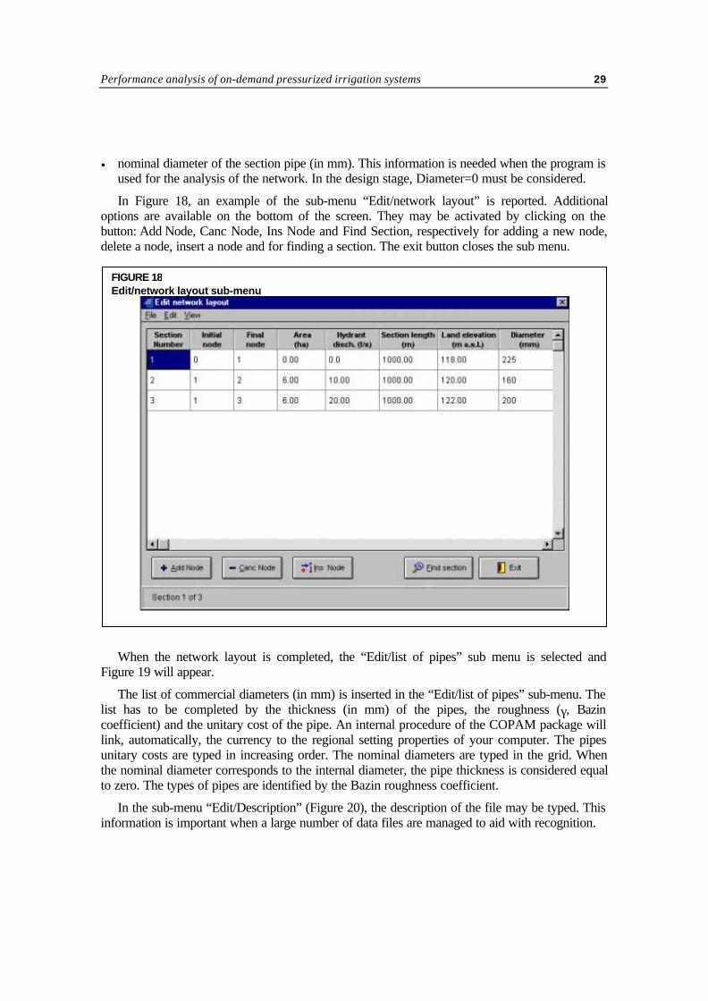
• area irrigated by each hydrant (in hectares); if no hydrant occurs in the node, Area=0 has tobe typed,
• hydrant discharge (in l s-1). It may be selected by clicking in the combo box,• section length (in m),• land elevation of the downstream node (in m a.s.l.),
FIGURE 17Examples of node numbering
Performance analysis of on-demand pressurized irrigation systems 29
• nominal diameter of the section pipe (in mm). This information is needed when the program isused for the analysis of the network. In the design stage, Diameter=0 must be considered.
In Figure 18, an example of the sub-menu “Edit/network layout” is reported. Additionaloptions are available on the bottom of the screen. They may be activated by clicking on thebutton: Add Node, Canc Node, Ins Node and Find Section, respectively for adding a new node,delete a node, insert a node and for finding a section. The exit button closes the sub menu.
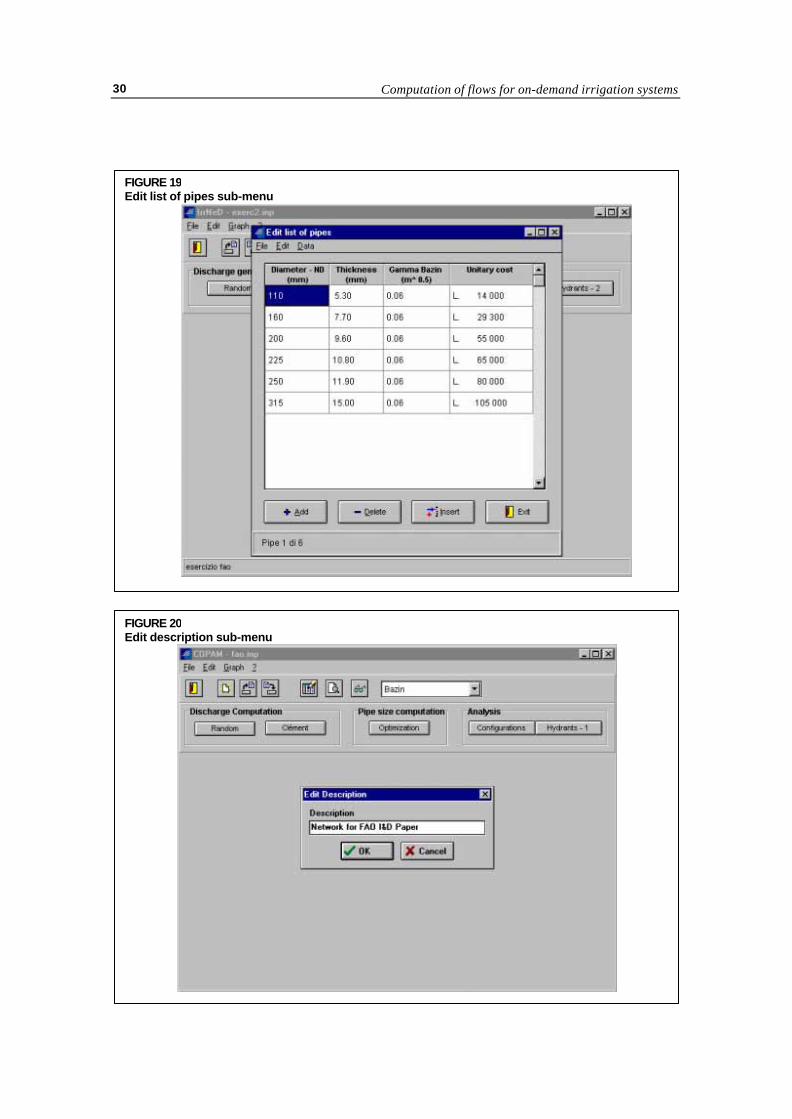
When the network layout is completed, the “Edit/list of pipes” sub menu is selected andFigure 19 will appear.
The list of commercial diameters (in mm) is inserted in the “Edit/list of pipes” sub-menu. Thelist has to be completed by the thickness (in mm) of the pipes, the roughness (γ, Bazincoefficient) and the unitary cost of the pipe. An internal procedure of the COPAM package willlink, automatically, the currency to the regional setting properties of your computer. The pipesunitary costs are typed in increasing order. The nominal diameters are typed in the grid. Whenthe nominal diameter corresponds to the internal diameter, the pipe thickness is considered equalto zero. The types of pipes are identified by the Bazin roughness coefficient.
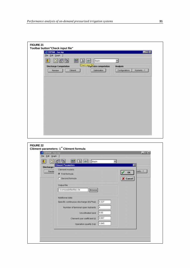
In the sub-menu “Edit/Description” (Figure 20), the description of the file may be typed. Thisinformation is important when a large number of data files are managed to aid with recognition.
FIGURE 18Edit/network layout sub-menu
Computation of flows for on-demand irrigation systems30
FIGURE 19Edit list of pipes sub-menu
FIGURE 20Edit description sub-menu
Performance analysis of on-demand pressurized irrigation systems 31
FIGURE 21Toolbar button”Check input file”
FIGURE 22Clément parameters: 1
st Clément formula
Computation of flows for on-demand irrigation systems32
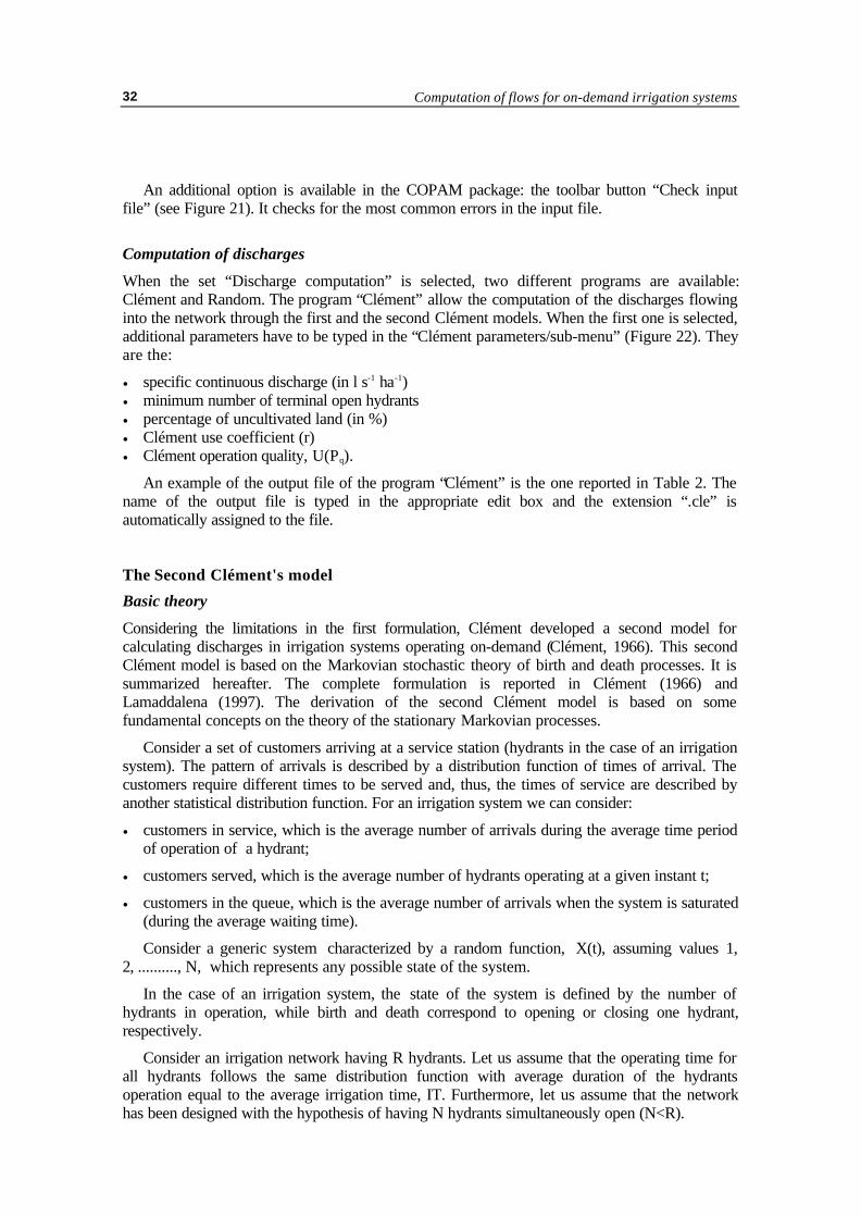
An additional option is available in the COPAM package: the toolbar button “Check inputfile” (see Figure 21). It checks for the most common errors in the input file.
Computation of discharges
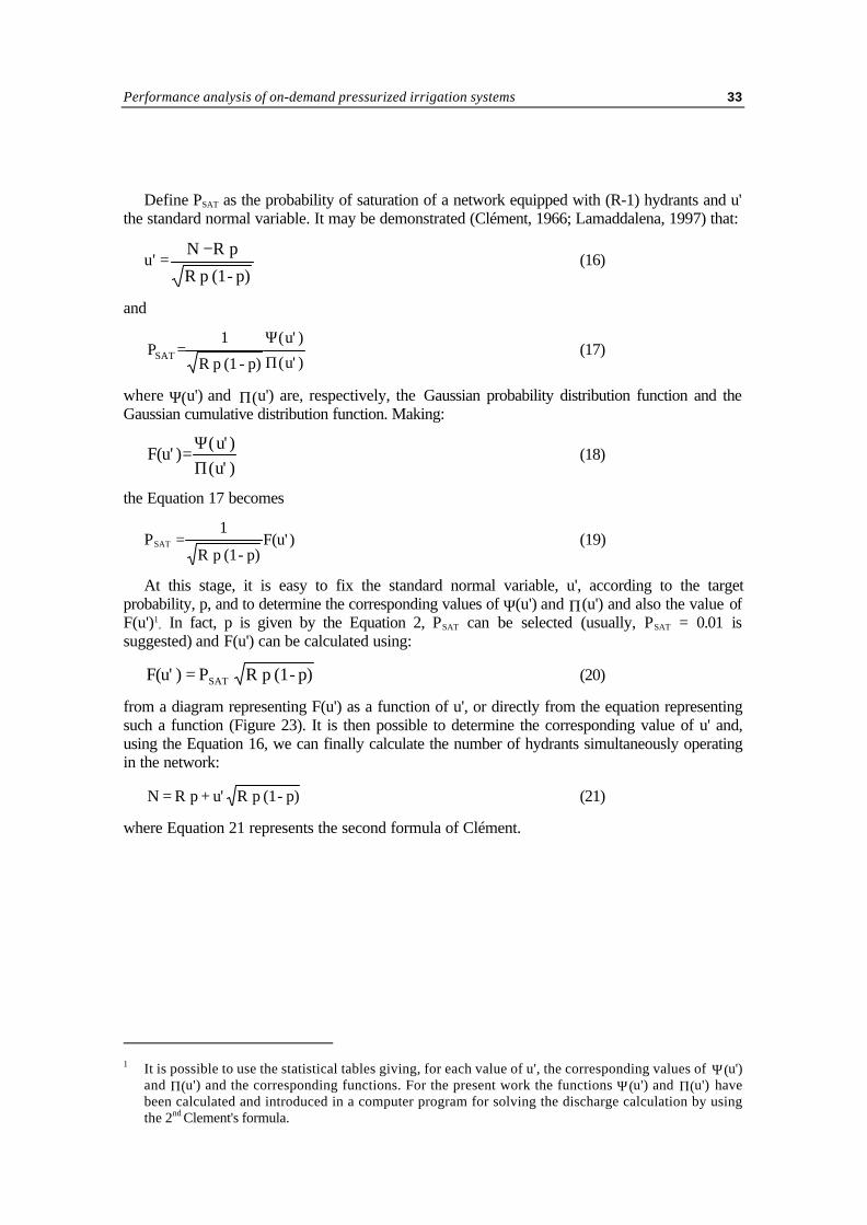
When the set “Discharge computation” is selected, two different programs are available:Clément and Random. The program “Clément” allow the computation of the discharges flowinginto the network through the first and the second Clément models. When the first one is selected,additional parameters have to be typed in the “Clément parameters/sub-menu” (Figure 22). Theyare the:
• specific continuous discharge (in l s-1 ha-1)• minimum number of terminal open hydrants• percentage of uncultivated land (in %)• Clément use coefficient (r)• Clément operation quality, U(Pq).
An example of the output file of the program “Clément” is the one reported in Table 2. Thename of the output file is typed in the appropriate edit box and the extension “.cle” isautomatically assigned to the file.
The Second Clément's model
Basic theory
Considering the limitations in the first formulation, Clément developed a second model forcalculating discharges in irrigation systems operating on-demand (Clément, 1966). This secondClément model is based on the Markovian stochastic theory of birth and death processes. It issummarized hereafter. The complete formulation is reported in Clément (1966) andLamaddalena (1997). The derivation of the second Clément model is based on somefundamental concepts on the theory of the stationary Markovian processes.
Consider a set of customers arriving at a service station (hydrants in the case of an irrigationsystem). The pattern of arrivals is described by a distribution function of times of arrival. Thecustomers require different times to be served and, thus, the times of service are described byanother statistical distribution function. For an irrigation system we can consider:
• customers in service, which is the average number of arrivals during the average time periodof operation of a hydrant;
• customers served, which is the average number of hydrants operating at a given instant t;
• customers in the queue, which is the average number of arrivals when the system is saturated(during the average waiting time).
Consider a generic system characterized by a random function, X(t), assuming values 1,2, .........., N, which represents any possible state of the system.
In the case of an irrigation system, the state of the system is defined by the number ofhydrants in operation, while birth and death correspond to opening or closing one hydrant,respectively.
Consider an irrigation network having R hydrants. Let us assume that the operating time forall hydrants follows the same distribution function with average duration of the hydrantsoperation equal to the average irrigation time, IT. Furthermore, let us assume that the networkhas been designed with the hypothesis of having N hydrants simultaneously open (N<R).
Performance analysis of on-demand pressurized irrigation systems 33
Define PSAT as the probability of saturation of a network equipped with (R-1) hydrants and u'the standard normal variable. It may be demonstrated (Clément, 1966; Lamaddalena, 1997) that:
u' =p)-(1 p R
p RN − (16)
and
)u'
)u'
p)-(1 p R
1=PSAT (Π
(Ψ (17)
where Ψ(u') and Π(u') are, respectively, the Gaussian probability distribution function and theGaussian cumulative distribution function. Making:
)u')u'
=)F(u'(Π(Ψ
(18)
the Equation 17 becomes
PSAT )F(u'p)-(1 p R
1= (19)
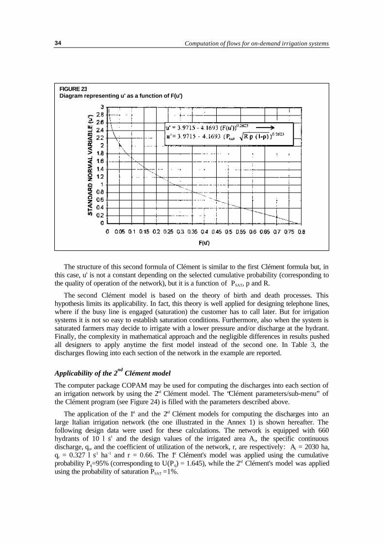
At this stage, it is easy to fix the standard normal variable, u', according to the targetprobability, p, and to determine the corresponding values of Ψ(u') and Π(u') and also the value ofF(u')1. In fact, p is given by the Equation 2, PSAT can be selected (usually, PSAT = 0.01 issuggested) and F(u') can be calculated using:
p)-(1 p R P = )F(u' SAT (20)
from a diagram representing F(u') as a function of u', or directly from the equation representingsuch a function (Figure 23). It is then possible to determine the corresponding value of u' and,using the Equation 16, we can finally calculate the number of hydrants simultaneously operatingin the network:
p)-(1 p R u' + p R = N (21)
where Equation 21 represents the second formula of Clément.
1 It is possible to use the statistical tables giving, for each value of u', the corresponding values of Ψ(u')
and Π(u') and the corresponding functions. For the present work the functions Ψ(u') and Π(u') havebeen calculated and introduced in a computer program for solving the discharge calculation by usingthe 2nd Clement's formula.
Computation of flows for on-demand irrigation systems34
The structure of this second formula of Clément is similar to the first Clément formula but, inthis case, u' is not a constant depending on the selected cumulative probability (corresponding tothe quality of operation of the network), but it is a function of PSAT, p and R.
The second Clément model is based on the theory of birth and death processes. Thishypothesis limits its applicability. In fact, this theory is well applied for designing telephone lines,where if the busy line is engaged (saturation) the customer has to call later. But for irrigationsystems it is not so easy to establish saturation conditions. Furthermore, also when the system issaturated farmers may decide to irrigate with a lower pressure and/or discharge at the hydrant.Finally, the complexity in mathematical approach and the negligible differences in results pushedall designers to apply anytime the first model instead of the second one. In Table 3, thedischarges flowing into each section of the network in the example are reported.
Applicability of the 2nd Clément model
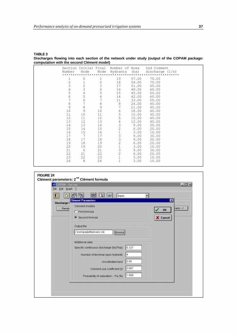
The computer package COPAM may be used for computing the discharges into each section ofan irrigation network by using the 2nd Clément model. The “Clément parameters/sub-menu” ofthe Clément program (see Figure 24) is filled with the parameters described above.
The application of the 1st and the 2nd Clément models for computing the discharges into anlarge Italian irrigation network (the one illustrated in the Annex 1) is shown hereafter. Thefollowing design data were used for these calculations. The network is equipped with 660hydrants of 10 l s-1 and the design values of the irrigated area Ai, the specific continuousdischarge, qs, and the coefficient of utilization of the network, r, are respectively: Ai = 2030 ha,qs = 0.327 l s-1 ha-1 and r = 0.66. The 1st Clément's model was applied using the cumulativeprobability Pq=95% (corresponding to U(Pq) = 1.645), while the 2nd Clément's model was appliedusing the probability of saturation PSAT =1%.
FIGURE 23Diagram representing u' as a function of F(u')
Performance analysis of on-demand pressurized irrigation systems 35
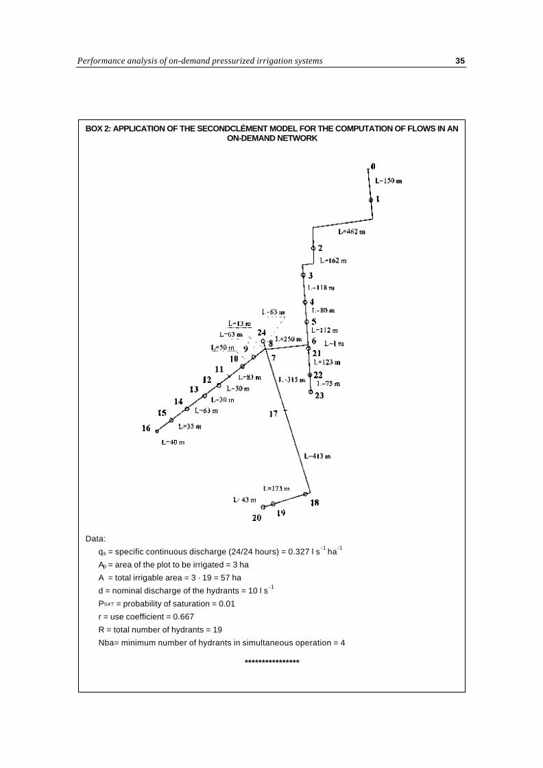
BOX 2: APPLICATION OF THE SECONDCLÉMENT MODEL FOR THE COMPUTATION OF FLOWS IN ANON-DEMAND NETWORK
Data:
qs = specific continuous discharge (24/24 hours) = 0.327 l s -1 ha-1
Ap = area of the plot to be irrigated = 3 ha
A = total irrigable area = 3 · 19 = 57 ha
d = nominal discharge of the hydrants = 10 l s -1
PSAT = probability of saturation = 0.01
r = use coefficient = 0.667
R = total number of hydrants = 19
Nba= minimum number of hydrants in simultaneous operation = 4
****************

Computation of flows for on-demand irrigation systems36
_________________________________1 In this example the mathematical approximation was used for computing the discharges in each section of the
network.
BOX 2 Cont’d
p = elementary probability =dRr
Asq=
10 19 0.667
57 0.327
⋅⋅
⋅= 0.147
u’ = standard normal variable = 3.9715 – 4.1693 ( PSAT p)-(1 pR )0.2623
1) Number of hydrants simultaneously operating downstream the section 0-1:
N0-1 = p)-(1 pRu'pR + =
[ ]{ } 0.147)-(1 0.147 190.2623
0.147)-(1 0.147 19 0.01 ( 4.1693 - 3.9715 0.147 19 ⋅⋅⋅⋅+⋅
= 6.77
We assume N 0-1 = 7 1
The design discharge downstream the section 0-1 is:
Q0-1 = N0-1 · d = 7 · 10 = 70 l s -1
2) Number of hydrants in simultaneous operation downstream the section 1-2:
N1-2 = p)-(1 pRu'pR + =
[ ]{ } 0.147)-(1 0.147 180.2623
0.147)-(1 0.147 18 0.01 ( 4.1693 - 3.9715 0.147 18 ⋅⋅⋅⋅+⋅ =
= 6.53
We assume N 1-2 = 7
The design discharge downstream the section 1-2 is:
Q1-2 = N1-2 · d = 7 · 10 = 70 l s -1
3) Number of hydrants in simultaneous operation downstream the section 2-3:
N2-3 = p)-(1 pRu'pR + =
[ ]{ } 0.147)-(1 0.147 170.2623
0.147)-(1 0.147 17 0.01 ( 4.1693 - 3.9715 0.147 17 ⋅⋅⋅⋅+⋅ =
6.29
We assume N 2-3 = 6
The design discharge downstream the section 2-3 is:
Q2-3 = N2-3 · d = 6 · 10 = 60 l s -1,
and so on for the calculation of the discharges in the other sections.
Performance analysis of on-demand pressurized irrigation systems 37
TABLE 3Discharges flowing into each section of the network under study (output of the COPAM package:computation with the second Clément model)
Section Initial Final Number of Area 2nd ClémentNumber Node Node Hydrants (ha) discharge (l/s)******************************************************** 1 0 1 19 57.00 70.00 2 1 2 18 54.00 70.00 3 2 3 17 51.00 60.00 4 3 4 16 48.00 60.00 5 4 5 15 45.00 60.00 6 5 6 14 42.00 60.00 7 6 7 11 33.00 50.00 8 7 8 8 24.00 40.00 9 8 9 7 21.00 40.00 10 9 10 6 18.00 40.00 11 10 11 5 15.00 40.00 12 11 12 5 15.00 40.00 13 12 13 4 12.00 40.00 14 13 14 3 9.00 30.00 15 14 15 2 6.00 20.00 16 15 16 1 3.00 10.00 17 7 17 3 9.00 30.00 18 17 18 3 9.00 30.00 19 18 19 2 6.00 20.00 20 19 20 1 3.00 10.00 21 6 21 3 9.00 30.00 22 21 22 2 6.00 20.00 23 22 23 1 3.00 10.00 24 8 24 1 3.00 10.00
FIGURE 24Clément parameters: 2nd Clément formula
Computation of flows for on-demand irrigation systems38
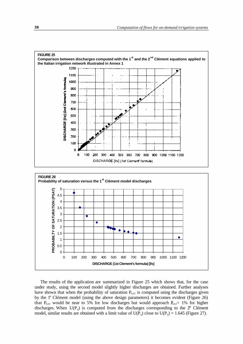
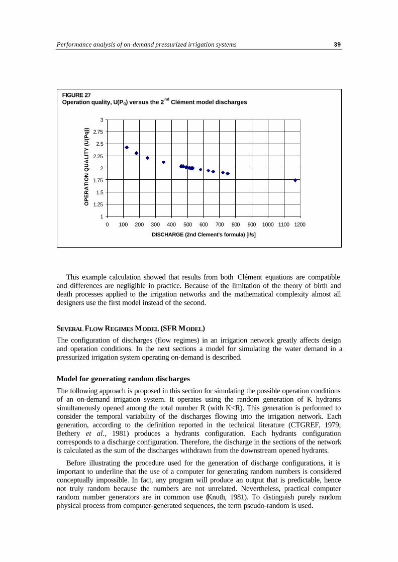
The results of the application are summarized in Figure 25 which shows that, for the caseunder study, using the second model slightly higher discharges are obtained. Further analyseshave shown that when the probability of saturation PSAT is computed using the discharges givenby the 1st Clément model (using the above design parameters) it becomes evident (Figure 26)that PSAT would be near to 5% for low discharges but would approach PSAT= 1% for higherdischarges. When U(Pq) is computed from the discharges corresponding to the 2nd Clémentmodel, similar results are obtained with a limit value of U(Pq) close to U(Pq) = 1.645 (Figure 27).
DISCHARGE [l/s] (1st Clement' formula)
FIGURE 25Comparison between discharges computed with the 1st and the 2nd Clément equations applied tothe Italian irrigation network illustrated in Annex 1
FIGURE 26Probability of saturation versus the 1st Clément model discharges
0
0.5
1
1.5
2
2.5
3
3.5
4
4.5
5
0 100 200 300 400 500 600 700 800 900 1000 1100 1200
DISCHARGE (1st Clement's formula) [l/s]
PR
OB
AB
ILT
Y O
F S
AT
UR
AT
ION
(PS
AT
)
Performance analysis of on-demand pressurized irrigation systems 39
This example calculation showed that results from both Clément equations are compatibleand differences are negligible in practice. Because of the limitation of the theory of birth anddeath processes applied to the irrigation networks and the mathematical complexity almost alldesigners use the first model instead of the second.
SEVERAL FLOW REGIMES MODEL (SFR MODEL)
The configuration of discharges (flow regimes) in an irrigation network greatly affects designand operation conditions. In the next sections a model for simulating the water demand in apressurized irrigation system operating on-demand is described.
Model for generating random discharges
The following approach is proposed in this section for simulating the possible operation conditionsof an on-demand irrigation system. It operates using the random generation of K hydrantssimultaneously opened among the total number R (with K<R). This generation is performed toconsider the temporal variability of the discharges flowing into the irrigation network. Eachgeneration, according to the definition reported in the technical literature (CTGREF, 1979;Bethery et al., 1981) produces a hydrants configuration. Each hydrants configurationcorresponds to a discharge configuration. Therefore, the discharge in the sections of the networkis calculated as the sum of the discharges withdrawn from the downstream opened hydrants.
Before illustrating the procedure used for the generation of discharge configurations, it isimportant to underline that the use of a computer for generating random numbers is consideredconceptually impossible. In fact, any program will produce an output that is predictable, hencenot truly random because the numbers are not unrelated. Nevertheless, practical computerrandom number generators are in common use (Knuth, 1981). To distinguish purely randomphysical process from computer-generated sequences, the term pseudo-random is used.
FIGURE 27Operation quality, U(Pq) versus the 2nd Clément model discharges
1
1.25
1.5
1.75
2
2.25
2.5
2.75
3
0 100 200 300 400 500 600 700 800 900 1000 1100 1200
DISCHARGE (2nd Clement's formula) [l/s]
OP
ER
AT
ION
QU
AL
ITY
(U
(Pq
))
Computation of flows for on-demand irrigation systems40
There exists a body of random number generators which mutually do satisfy the definitionover a very broad class of application programs. But what is random enough for one applicationmay not be random enough for another. The chi-square test may be used to verify the goodnessof the random generation for a particular application (Press et al., 1989; Knuth, 1981).
For generating random discharge configurations, uniform deviates are applied. The uniformdeviates are just random numbers which lie within a specified range, with any one randomnumber in the range just as likely as any other (Press et al., 1989).
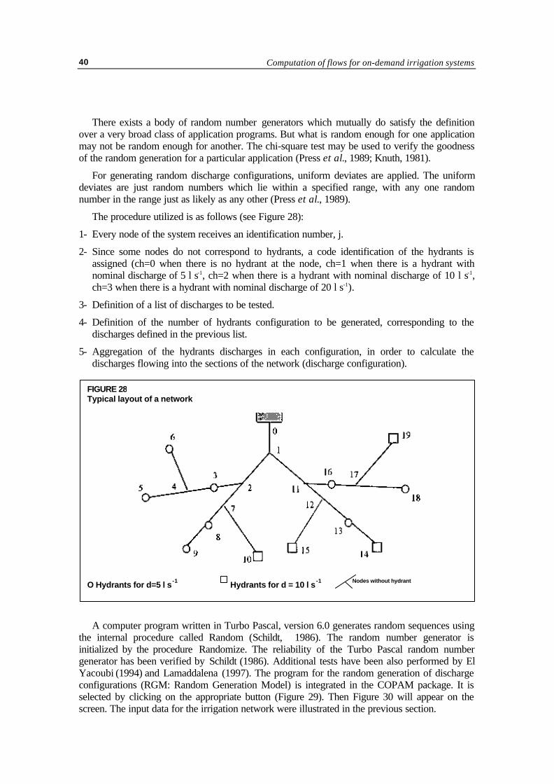
The procedure utilized is as follows (see Figure 28):
1- Every node of the system receives an identification number, j.
2- Since some nodes do not correspond to hydrants, a code identification of the hydrants isassigned (ch=0 when there is no hydrant at the node, ch=1 when there is a hydrant withnominal discharge of 5 l s-1, ch=2 when there is a hydrant with nominal discharge of 10 l s-1,ch=3 when there is a hydrant with nominal discharge of 20 l s-1).
3- Definition of a list of discharges to be tested.
4- Definition of the number of hydrants configuration to be generated, corresponding to thedischarges defined in the previous list.
5- Aggregation of the hydrants discharges in each configuration, in order to calculate thedischarges flowing into the sections of the network (discharge configuration).
A computer program written in Turbo Pascal, version 6.0 generates random sequences usingthe internal procedure called Random (Schildt, 1986). The random number generator isinitialized by the procedure Randomize. The reliability of the Turbo Pascal random numbergenerator has been verified by Schildt (1986). Additional tests have been also performed by ElYacoubi (1994) and Lamaddalena (1997). The program for the random generation of dischargeconfigurations (RGM: Random Generation Model) is integrated in the COPAM package. It isselected by clicking on the appropriate button (Figure 29). Then Figure 30 will appear on thescreen. The input data for the irrigation network were illustrated in the previous section.
FIGURE 28Typical layout of a network
O Hydrants for d=5 l s -1 Hydrants for d = 10 l s -1 Nodes without hydrant

Performance analysis of on-demand pressurized irrigation systems 41
The RG Model may be used for two different purposes:
• analysis of existing irrigation systems;• design of new irrigation systems.
In the first case, this model is based on the knowledge of the demand hydrograph at theupstream end of the network. In fact, it allows the selection of the upstream dischargecorresponding to various hydrant configurations. The value of the upstream discharge is insertedin the appropriate edit box (see Figure 30). Corresponding to the selected discharge, a number ofhydrants simultaneously operating (hydrant configuration) is automatically withdrawn. Thisprocedure is repeated for several configurations and is used for analysing the system, asillustrated in the chapter 5. The number of configurations (or flow regimes) to generate is typedin the appropriate edit box (see Figure 30). It must be multiple of 10.
All the generated flow regimes are stored in an output file with its name typed in theappropriate edit box. The extension “.ran” is automatically assigned to this output file.
When a new irrigation system is designed, the upstream discharge is not known a priori.Therefore, to allow the generation of different hydrants configurations, such discharge may becomputed, for example, with the Clément models1. This is achieved through the COPAM
1 Other models for generating the upstream discharges are under study. Nevertheless, despite the good
improvements that have been made in the generation of the upstream withdrawn volumes, the problemof transformation from volumes to discharges has still not been solved because of a number of
FIGURE 29Random generation program
Computation of flows for on-demand irrigation systems42
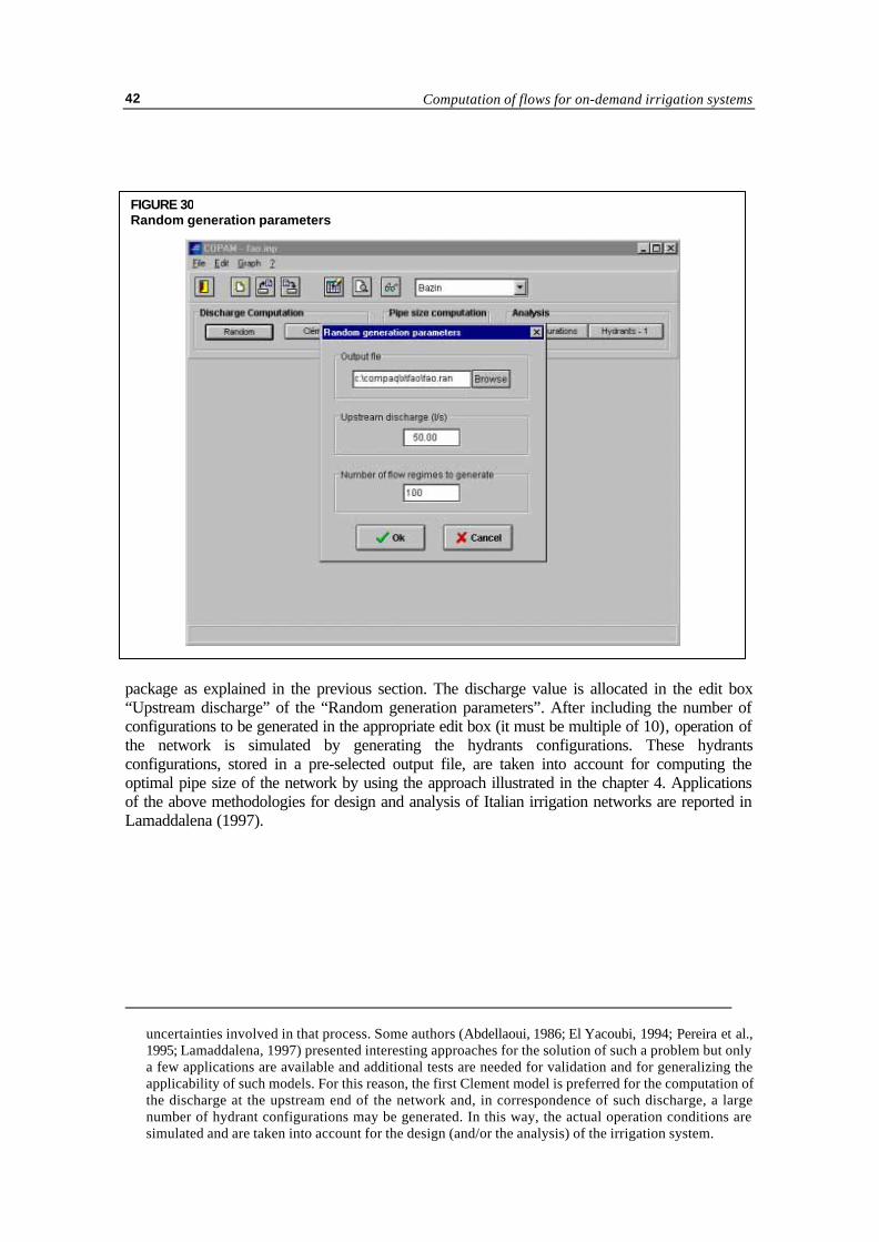
package as explained in the previous section. The discharge value is allocated in the edit box“Upstream discharge” of the “Random generation parameters”. After including the number ofconfigurations to be generated in the appropriate edit box (it must be multiple of 10), operation ofthe network is simulated by generating the hydrants configurations. These hydrantsconfigurations, stored in a pre-selected output file, are taken into account for computing theoptimal pipe size of the network by using the approach illustrated in the chapter 4. Applicationsof the above methodologies for design and analysis of Italian irrigation networks are reported inLamaddalena (1997).
uncertainties involved in that process. Some authors (Abdellaoui, 1986; El Yacoubi, 1994; Pereira et al.,1995; Lamaddalena, 1997) presented interesting approaches for the solution of such a problem but onlya few applications are available and additional tests are needed for validation and for generalizing theapplicability of such models. For this reason, the first Clement model is preferred for the computation ofthe discharge at the upstream end of the network and, in correspondence of such discharge, a largenumber of hydrant configurations may be generated. In this way, the actual operation conditions aresimulated and are taken into account for the design (and/or the analysis) of the irrigation system.
FIGURE 30Random generation parameters
Performance analysis of on-demand pressurized irrigation systems 43
Chapter 4
Pipe-size calculation
The problem of calculating the optimal pipe size diameters of an irrigation network has attractedthe attention of many researchers and designers. Many optimization models based on linearprogramming (LP), non-linear programming (NLP) and dynamic programming (DP) techniquesare available in literature. These models give important improvements to practical problemsthrough less costly solutions and less computation time respect to the classical approaches.
One limitation of the optimization models is that they consider only One Flow Regime(OFR) during the process of the pipe size computation. With this kind of approach, there is noassurance that the system selected is the least costly and compatible with the requiredperformance. Indeed, in on-demand irrigation systems, the distribution of flows in each sectionmay strongly vary in time and space. Thus, several flow regimes (SFR) should be taken intoaccount during the computation process.
In this chapter an optimization model using the Labye's Iterative discontinuous algorithm ispresented and applied for the case of One Flow Regime and extended to the case of SeveralFlow Regimes.
OPTIMIZATION OF PIPE DIAMETERS WITH OFRM
Review on optimization procedures
Research on optimization procedures to design water distribution networks have been reportedsince the 1960s. Karmeli et al. (1968), Schaake and Lai (1969), and Lieng (1971) developedoptimization models for solving branched networks where a given demand pattern was used todefine the flow uniquely in the pipes. Afterwards, important efforts have been made byAlperovits and Shamir (1977), Quindri et al. (1981), Morgan and Goulter (1985) for solvinglooped systems, where infinite number of distributions of flow can meet a specific demandpattern. Alperovits and Shamir (1977) used fundamental linear programming formulation buttheir approach is severely limited to small size systems. The approach by Quindri et al. (1981)may solve larger systems but only pipes are included in the design and no additionalcomponents are considered (e.g. pumping station, reservoirs, valves). In the approach byMorgan and Goulter (1985). the cost of components is not included in the objective function andmultiple runs are required to determine the best solution.
Lansey and Mays (1989) proposed a methodology for determining the optimal design ofwater distribution systems considering the pipe size, the pumping station and reservoirs. Inaddition, the optimal setting for control and pressure-reducing valves can be determined. Thismethodology considers the design problem as a non-linear one, where all the typicalcomponents of a network are designed while analyzing multiple alternative discharges. Thisprocedure still is computationally intensive and requires a large number of iterations to obtainthe solution, especially when applied to large networks.
Pipe-size calculation44
In view of the concerns sometimes expressed about the use of linear programming whenlarge networks are designed, other approaches have been developed (Labye, 1966 and 1981)using the dynamic programming formulation. Later, another approach was developed (Ait Kadi,1986) to optimize the network layout and the pipe sizes simultaneously for a network composedby a mainline and secondary parallel branches. This approach (Ait Kadi, 1986) involves twostages. In the first one, an initial solution is constructed by obtaining the optimum layout of themainline, with each pipe of the network having the smallest allowable diameter. In the secondstage, the initial solution is improved by reducing, iteratively, the upstream head and,consequently, varying the layout of the mainline and pipe sizes simultaneously. This iterativeprocess is continued until the optimum head giving the minimum cost of the network is reached.
In recent years, several comprehensive reviews on the state-of-the-art in this field wereundertaken (Walsky, 1985b; Goulter, 1987; Walters, 1988). Furthermore, a number ofoptimization models were assessed (Walsky et al., 1987). An interesting result of the analysisby Walsky et al. (1987) was that models produce similar design, both in terms of costs andhardware components selected. The cost associated with the solutions determined by differentmodels only varied by 12%. In addition, the most expensive systems were those with increasedlevel of reliability, imparted by additional storage in the system. Linear programming anddynamic programming for calculating the optimal pipe diameters in irrigation networks havealso been compared (Di Santo and Petrillo, 1980a,b; Ait Kadi, 1986).
Di Santo and Petrillo (1980a) demonstrated that a network solved by using both LP and theDP with Bellman's formulation has the same optimal solution. Results obtained by Ait Kadi(1986) for networks solved by using both LP and the Labye's Iterative Discontinuos Method(LIDM) were similar.
The above analyses (Di Santo and Petrillo, 1980a,b; Ait Kadi, 1986; Walsky et al., 1987)indicate that the optimization models utilized were relatively robust and that the optimization isnot sensitive to the technique itself. However, it is useful to improve the ability to design andanalyze water distribution systems. In fact, system design must consider various critical demandhydrographs to ensure system reliability (Templeman, 1982; Hashimoto et al., 1982). This isvalid for both branched and looped networks where the same daily pattern demand maycorrespond to several configurations of flows in the pipes. In addition, it is useful to examine theextent to which the model techniques and approaches are incorporated into engineering practice.
Better designs have been obtained through optimization models but there has been noguarantee of global optimality, i.e. on what should be the objective of an optimal design.Assuming that an optimal design is the one which meets the applied demands at the least cost(Goulter, 1992), it should incorporate multiple demand conditions, failures in the systemcomponents and reliability.
For considering the reliability of the network, a definition of "failure" is necessary. Ingeneral, a network failure is an event in which a network is not able to provide sufficient flow orsufficient pressure to meet the demand. Under this definition, failure can occur either if acomponent (e.g., a pipe) is undersized, or if the actual demand exceeds the design demand.These two cases are independent for practical purposes. A considerable effort has been directedto the reliability question over the last few years.
Relatively little success has been achieved in obtaining comprehensive measures of networkreliability that are computationally feasible and physically realistic (Goulter, 1987; Lansey andBasnet, 1990).
The measures that give good representation of reliability are computationally impractical,like the model by Su et al. (1987) where 200 min. of computer time is needed for solving a three
Performance analysis of on-demand pressurized irrigation systems 45
loop example. On the other hand, those approaches that are computationally suitable providevery poor description of the network performance. Also, empirical solutions may be consideredfor improving reliability performance, like the one by Bouchard and Goulter (1991) whichproposed to add valves to the links in order to isolate branches during failure for repair.
Despite the efforts in developing optimization models, they are not widely used in practice.The main reasons for this are: they are often too complex to be used and designers are notcomfortable with the optimization approaches.
Indeed, Walsky et al. (1987) have shown that, by using optimization models, importantanswers to practical problems are possible which can be verified using simulation techniques.Furthermore, optimization models require less computation time than the classical approaches.Usually, optimization models are difficult to use. The main reason is that they are developed inacademic environments where the algorithm is much more important than the input-outputinterface. In addition, many older engineers have not had opportunity to study formaloptimization techniques.
Considering the effort in developing optimization models, it seems reasonable to assert thatresearch should be oriented to integrate simulation and optimization models rather than todevelop new optimization algorithms. Techniques for designing optimal pipe diameters forirrigation networks under several discharge configurations need to be improved and tested.Furthermore, reliability of systems need to be well defined in order to be included in theoptimization process. Finally, the need for improving the user interface in optimization modelssoftware is important (Walsky et al., 1987).
An interesting commercial program for the calculation of the optimal pipe diameters forirrigation networks has been developed by CEMAGREF (1990). This program (XERXES-RENFORS, vers. 5.0) has a user-friendly interface. It computes the discharges with the firstClément formula, or by adding hydrants' discharges, while Labye's discontinuous method isused to compute the optimal diameters. Also, optimal pumping station and optimalreinforcement of the networks may be calculated. This program has interfaces in French andhead losses are computed using the Calmon and Lechapt formula.
In the present publication, an effort has been made to develop and distribute the computerprogram (COPAM). It has an English user-friendly interface and all the calculations are easy. Itintegrates models for the optimal pipe size computation with models for the analysis ofirrigation systems and allow to present the outputs under form of files and graphics. Theprogram facilitates full understanding by the user with the capability to verify the results.
When the design of the pumping stations is required the economic aspects are an importantcomponent but the performance analysis of the network is also required. This latter aspect iscovered in Chapter 5.
As far as the regulation of the pumping stations is concerned, the reader is referred toIrrigation and Drainage Paper No. 44 (page 128) where the subject is treated in detail. However,the regulation by variable speed pumps is a promising approach concerning energy saving andhas been detailed in Chapter 5 (page 74).
Labye's Iterative Discontinuous Method (LIDM) for OFRThe approach proposed by Labye (1981), called Labye's Iterative Discontinuous Method(LIDM), for optimizing pipe sizes in an irrigation network is described in this section. Thismethod is developed in two stages.
Pipe-size calculation46
In the first stage, an initial solution is constructed giving, for each section k of the network,the minimum commercial diameter (Dmin) according to the maximum allowable flow velocity(vmax) in a pipe, when the pipe conveys the calculated discharge (Qk). The diameter for thesection k is calculated by the relationship:
(Dmin)k = max
k
vp
Q4 (22)
After knowing the initial diameters, it is possible to calculate the piezometric elevation (Z0)in
at the upstream end of the network, which satisfies the minimum head (Hj,min) required at themost unfavorable hydrant (j):
(Z0)in = Hj,min + ZTj + Y k0 M j→∑ (23)
where Y k0 M j→∑ are the head losses along the pathway (Mj) connecting the upstream end of the
network to the most unfavourable hydrant.
The initial piezometric elevation (Z0)in relative to the initial diameters solution is thereforecalculated through the relationship (23).
In the second stage, the optimal solution is obtained by iteratively decreasing the upstreampiezometric elevation (Z0)in until reaching the effectively available upstream piezometricelevation, Z0, by selecting, for each iteration, the sections for which an increase in diameterproduces the minimum increase of the network cost. The selection process at each iteration iscarried out as described below.
At any iteration i, the commercial pipe diameters (at most two diameters per section (Labye,1966)) Ds+1 and Ds (with Ds+1 > Ds) are known. The coefficient:
β s =
P PJ J
s s
s s
+
+
−−1
1
(24)
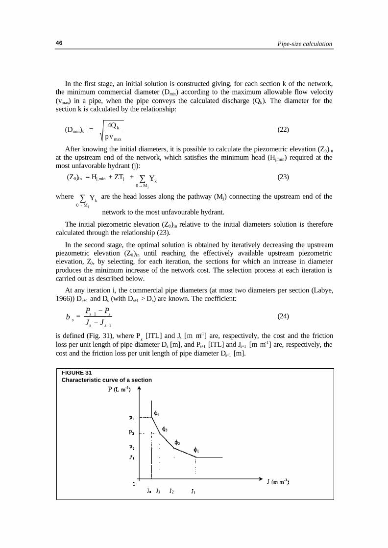
is defined (Fig. 31), where Ps
[ITL] and Js [m m-1] are, respectively, the cost and the frictionloss per unit length of pipe diameter Ds [m], and Ps+1 [ITL] and Js+1 [m m-1] are, respectively, thecost and the friction loss per unit length of pipe diameter Ds+1 [m].
FIGURE 31Characteristic curve of a section
Performance analysis of on-demand pressurized irrigation systems 47
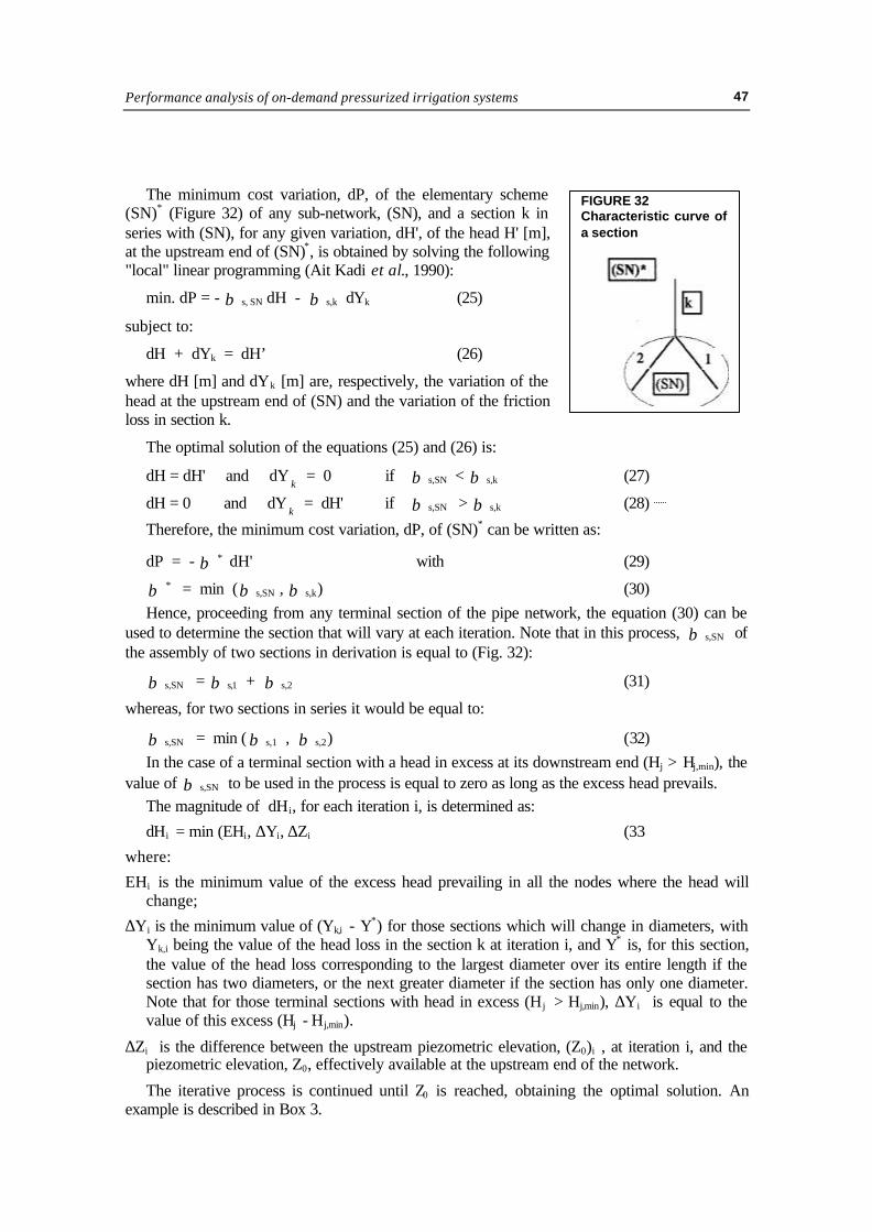
The minimum cost variation, dP, of the elementary scheme(SN)* (Figure 32) of any sub-network, (SN), and a section k inseries with (SN), for any given variation, dH', of the head H' [m],at the upstream end of (SN)*, is obtained by solving the following"local" linear programming (Ait Kadi et al., 1990):
min. dP = - β s, SN dH - β s,k dYk (25)
subject to:
dH + dYk = dH’ (26)
where dH [m] and dYk [m] are, respectively, the variation of thehead at the upstream end of (SN) and the variation of the frictionloss in section k.
The optimal solution of the equations (25) and (26) is:
dH = dH' and dYk
= 0 if β s,SN < β s,k (27)
dH = 0 and dYk
= dH' if β s,SN > β s,k (28)
Therefore, the minimum cost variation, dP, of (SN)* can be written as:
dP = - β * dH' with (29)
β * = min (β s,SN , β s,k) (30)Hence, proceeding from any terminal section of the pipe network, the equation (30) can be
used to determine the section that will vary at each iteration. Note that in this process, β s,SN ofthe assembly of two sections in derivation is equal to (Fig. 32):
β s,SN = β s,1 + β s,2 (31)
whereas, for two sections in series it would be equal to:
β s,SN = min ( β s,1 , β s,2) (32)In the case of a terminal section with a head in excess at its downstream end (Hj > Hj,min), the
value of β s,SN to be used in the process is equal to zero as long as the excess head prevails.The magnitude of dHi, for each iteration i, is determined as:
dHi = min (EHi, ∆Yi, ∆Zi) (33)
where:
EHi is the minimum value of the excess head prevailing in all the nodes where the head willchange;
∆Yi is the minimum value of (Yk,i - Y*) for those sections which will change in diameters, withYk,i being the value of the head loss in the section k at iteration i, and Y* is, for this section,the value of the head loss corresponding to the largest diameter over its entire length if thesection has two diameters, or the next greater diameter if the section has only one diameter.Note that for those terminal sections with head in excess (H j > Hj,min), ∆Yi is equal to thevalue of this excess (Hj - Hj,min).
∆Zi is the difference between the upstream piezometric elevation, (Z0)i , at iteration i, and thepiezometric elevation, Z0, effectively available at the upstream end of the network.
The iterative process is continued until Z0 is reached, obtaining the optimal solution. Anexample is described in Box 3.
FIGURE 32Characteristic curve ofa section
Pipe-size calculation48
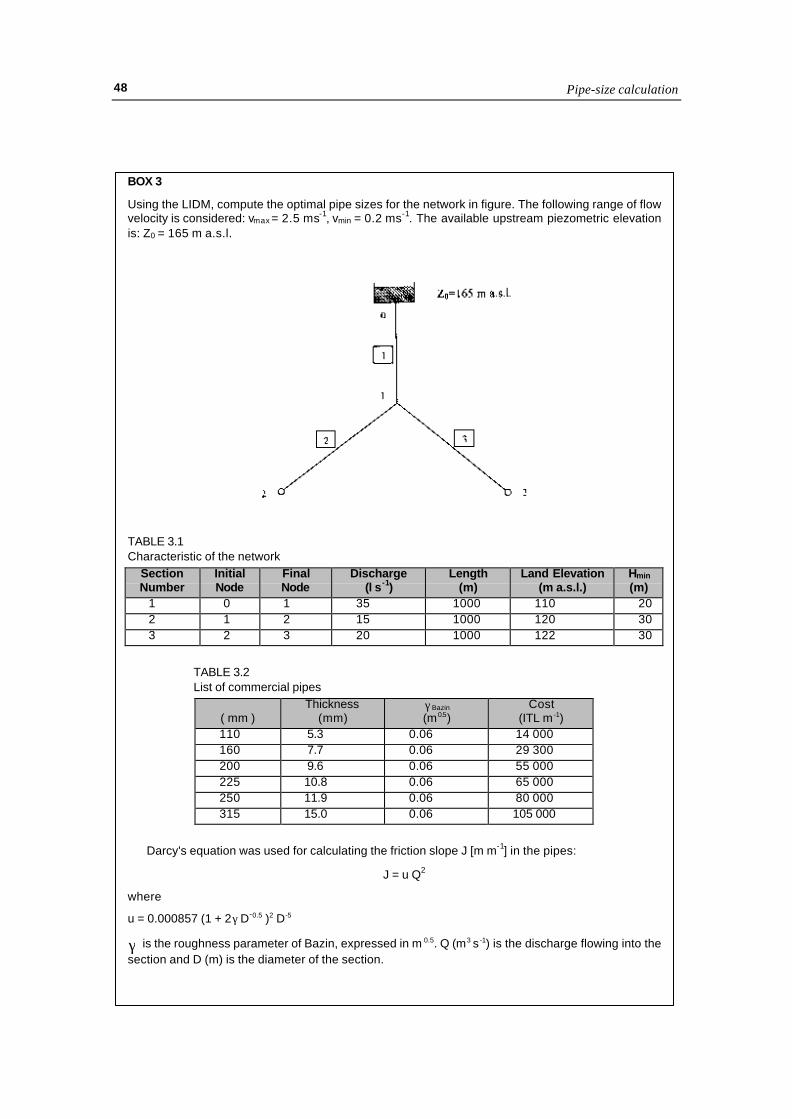
BOX 3
Using the LIDM, compute the optimal pipe sizes for the network in figure. The following range of flowvelocity is considered: vmax = 2.5 ms-1, vmin = 0.2 ms-1. The available upstream piezometric elevationis: Z0 = 165 m a.s.l.
TABLE 3.1Characteristic of the network
SectionNumber
InitialNode
FinalNode
Discharge(l s-1)
Length(m)
Land Elevation(m a.s.l.)
Hmin
(m)1 0 1 35 1000 110 202 1 2 15 1000 120 303 2 3 20 1000 122 30
TABLE 3.2List of commercial pipes
∅( mm )
Thickness(mm)
γ Bazin
(m0.5)Cost
(ITL m -1)110 5.3 0.06 14 000160 7.7 0.06 29 300200 9.6 0.06 55 000225 10.8 0.06 65 000250 11.9 0.06 80 000315 15.0 0.06 105 000
Darcy's equation was used for calculating the friction slope J [m m-1] in the pipes:
J = u Q2
where
u = 0.000857 (1 + 2γ D-0.5 )2 D-5
γ is the roughness parameter of Bazin, expressed in m 0.5. Q (m3 s -1) is the discharge flowing into thesection and D (m) is the diameter of the section.
Performance analysis of on-demand pressurized irrigation systems 49
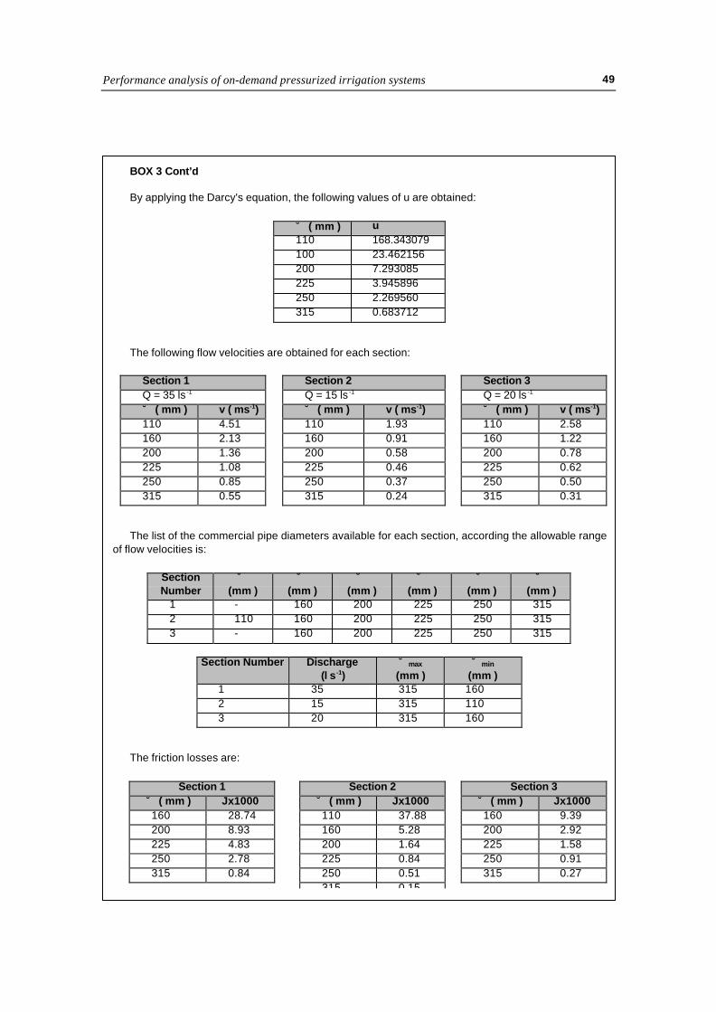
BOX 3 Cont’d
By applying the Darcy's equation, the following values of u are obtained:
∅ ( mm ) u110 168.343079100 23.462156200 7.293085225 3.945896250 2.269560315 0.683712
The following flow velocities are obtained for each section:
Section 1 Section 2 Section 3Q = 35 ls -1 Q = 15 ls -1 Q = 20 ls -1
∅ ( mm ) v ( ms-1) ∅ ( mm ) v ( ms-1) ∅ ( mm ) v ( ms-1)110 4.51 110 1.93 110 2.58160 2.13 160 0.91 160 1.22200 1.36 200 0.58 200 0.78225 1.08 225 0.46 225 0.62250 0.85 250 0.37 250 0.50315 0.55 315 0.24 315 0.31
The list of the commercial pipe diameters available for each section, according the allowable rangeof flow velocities is:
SectionNumber
∅(mm )
∅(mm )
∅(mm )
∅(mm )
∅(mm )
∅(mm )
1 - 160 200 225 250 3152 110 160 200 225 250 3153 - 160 200 225 250 315
Section Number Discharge(l s-1)
∅max
(mm )∅min
(mm )1 35 315 1602 15 315 1103 20 315 160
The friction losses are:
Section 1 Section 2 Section 3∅ ( mm ) Jx1000 ∅ ( mm ) Jx1000 ∅ ( mm ) Jx1000160 28.74 110 37.88 160 9.39200 8.93 160 5.28 200 2.92225 4.83 200 1.64 225 1.58250 2.78 225 0.84 250 0.91315 0.84 250 0.51 315 0.27
315 0.15
Pipe-size calculation50
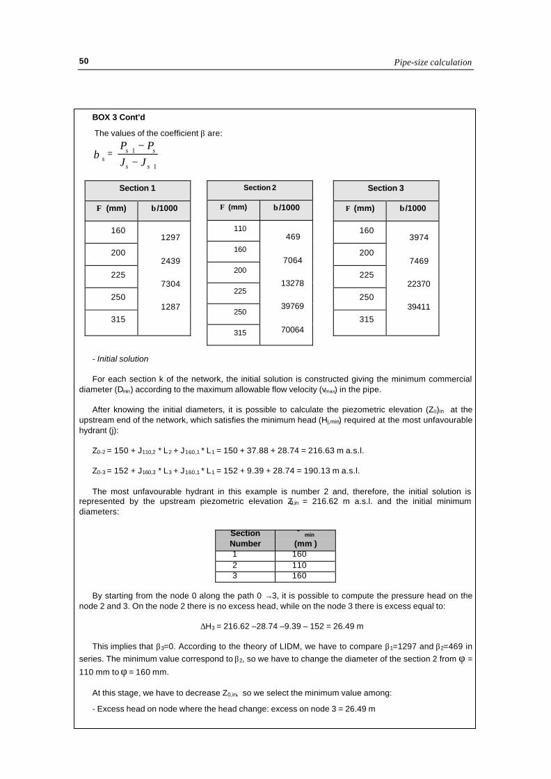
BOX 3 Cont’d
The values of the coefficient β are:
β s =
P PJ J
s s
s s
+
+
−−1
1
- Initial solution
For each section k of the network, the initial solution is constructed giving the minimum commercialdiameter (Dmin) according to the maximum allowable flow velocity (vmax) in the pipe.
After knowing the initial diameters, it is possible to calculate the piezometric elevation (Z0)in at the
upstream end of the network, which satisfies the minimum head (Hj,min) required at the most unfavourablehydrant (j):
Z0-2 = 150 + J110,2 * L2 + J160,1 * L1 = 150 + 37.88 + 28.74 = 216.63 m a.s.l.
Z0-3 = 152 + J160,3 * L3 + J160,1 * L1 = 152 + 9.39 + 28.74 = 190.13 m a.s.l.
The most unfavourable hydrant in this example is number 2 and, therefore, the initial solution isrepresented by the upstream piezometric elevation Z0,in = 216.62 m a.s.l. and the initial minimumdiameters:
SectionNumber
∅min
(mm )1 1602 1103 160
By starting from the node 0 along the path 0 →3, it is possible to compute the pressure head on thenode 2 and 3. On the node 2 there is no excess head, while on the node 3 there is excess equal to:
∆H3 = 216.62 –28.74 –9.39 – 152 = 26.49 m
This implies that β3=0. According to the theory of LIDM, we have to compare β1=1297 and β2=469 inseries. The minimum value correspond to β2, so we have to change the diameter of the section 2 from φ =
110 mm to φ = 160 mm.
At this stage, we have to decrease Z0,in, so we select the minimum value among:
- Excess head on node where the head change: excess on node 3 = 26.49 m
Section 1
Φ (mm) β /1000
160
200
225
250
315
1297
2439
7304
1287
Section 2
Φ (mm) β /1000
110
160
200
225
250
315
469
7064
13278
39769
70064
Section 3
Φ (mm) β /1000
160
200
225
250
315
3974
7469
22370
39411

Performance analysis of on-demand pressurized irrigation systems 51
BOX 3 Cont’d
- Z0,in – Z0 = 216.62 - 165 = 51.62 m
∆Y → by changing the diameter of the section 2 from φ = 110 mm to φ = 160 mm:
∆Y = 37.88 – 5.28 = 32.60 m
The minimum value is 26.49 m
- The solution at the first iteration is:
Z0,1 = 216.62 – 26.49 = 190.13 m a.s.l.
This gives the diameters shown below:
SectionNumber
∅min
(mm )1 1602 160 *3 160
* By changing the whole diameter on the section 2 we would recover 32.60 m and, in fact, we decreasethe upstream piezometric elevation only 26.49 m. This implies that we have a mixage on section 2between the diameters φ = 110 mm and φ = 160 mm. The lengths of such mixage are:
Note that 1000 / 32.60 = X / 26.49 and
This means that 813 m of the section 2 needs a diameter φ = 160 mm and (1000-813) = 187 m needs adiameter φ = 110 mm.
At this stage, there is no excess head on the nodes 2 and 3. Therefore, the sections 2 and 3 are inparallel, and the values of the coefficients β for identifying the sections to be changed are
- for the sections 2 and 3: β = β2 + β3 = 469 + 3974 = 4453
- for the sections 1: β1=1297
The minimum value is β1, therefore we have to increase the diameter on the section 1 from φ = 160 mm toφ = 200 mm.
m 81332.60
26.491000X =
⋅=
Pipe-size calculation52
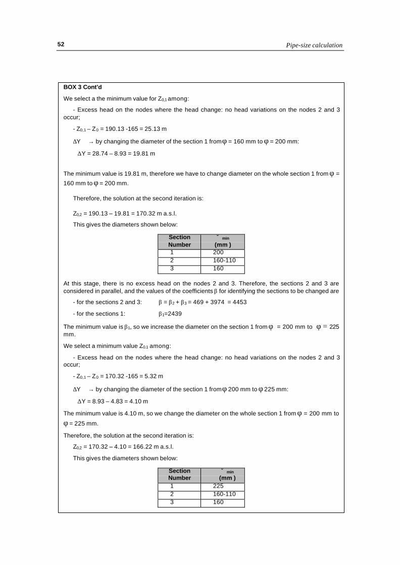
BOX 3 Cont’d
We select a the minimum value for Z0,1 among:
- Excess head on the nodes where the head change: no head variations on the nodes 2 and 3occur;
- Z0,1 – Z0 = 190.13 -165 = 25.13 m
∆Y → by changing the diameter of the section 1 from φ = 160 mm to φ = 200 mm:
∆Y = 28.74 – 8.93 = 19.81 m
The minimum value is 19.81 m, therefore we have to change diameter on the whole section 1 from φ =
160 mm to φ = 200 mm.
Therefore, the solution at the second iteration is:
Z0,2 = 190.13 – 19.81 = 170.32 m a.s.l.
This gives the diameters shown below:
SectionNumber
∅min
(mm )1 2002 160-1103 160
At this stage, there is no excess head on the nodes 2 and 3. Therefore, the sections 2 and 3 areconsidered in parallel, and the values of the coefficients β for identifying the sections to be changed are
- for the sections 2 and 3: β = β2 + β3 = 469 + 3974 = 4453
- for the sections 1: β1=2439
The minimum value is β1, so we increase the diameter on the section 1 from φ = 200 mm to φ = 225mm.
We select a minimum value Z0.1 among:
- Excess head on the nodes where the head change: no head variations on the nodes 2 and 3occur;
- Z0,1 – Z0 = 170.32 -165 = 5.32 m
∆Y → by changing the diameter of the section 1 from φ 200 mm to φ 225 mm:
∆Y = 8.93 – 4.83 = 4.10 m
The minimum value is 4.10 m, so we change the diameter on the whole section 1 from φ = 200 mm to
φ = 225 mm.
Therefore, the solution at the second iteration is:
Z0,2 = 170.32 – 4.10 = 166.22 m a.s.l.
This gives the diameters shown below:
SectionNumber
∅min
(mm )1 2252 160-1103 160

Performance analysis of on-demand pressurized irrigation systems 53
BOX 3 Cont’d
At this stage, there is still no any excess head on the nodes 2 and 3, so sections 2 and 3 areconsidered in parallel, and the values of the coefficients β for identifying the sections to be changed are
- for the sections 2 and 3: β = β2 + β3 = 469 + 3974 = 4453
- for the sections 1: β1=7304
The minimum value is β = β2 + β3, so we increase the diameter on the sections 2 and 3.
We select the minimum Z0,2 value among:
- Excess head on the nodes where the head change: no head variation on the nodes 2 and 3 occur;
- Z0,2 – Z0 = 66.22 -165 = 1.22 m
∆Y → by changing the diameter of the section 3 from φ = 160 mm to φ = 200 mm:
∆Y3 = 9.38 – 2.92 = 6.46 m
∆Y → by changing the whole diameter of the section 2 from φ = 110 mm to φ = 160 mm:
∆Y2 = 32.60 – 26.49 = 6.11 m
The minimum value is 1.22 m, so we change part of the diameter φ = 110 mm in the section 2 to φ =
160 mm and we change part of the diameter φ = 160 mm in the section 3 into φ = 200 mm. We willhave mixage on the sections 2 and 3.
The solution at the third iteration is:
Z0,3 = 166.22 – 1.22 = 165 m a.s.l.
This gives the diameters shown below:
SectionNumber
∅min
(mm )1 2252 160-1103 200-160
Mixage on the section 3:
Note that 1000 / 6.47 = X / 1.22, so
m 1896.47
1.221000X =
⋅=
This means that 189 m of the section 3 needs a diameter φ = 200 mm and (1000-189) = 811 m
needs a diameter φ = 160 mm.

Pipe-size calculation54
OPTIMIZATION OF PIPE DIAMETERS WITH SFRM
The above described optimization method considers fixed discharges flowing into the pipes ofthe network. This is not true for irrigation systems, especially when on-demand deliveryschedules are adopted. In these systems, the discharges are strongly variable in time because ofthe extreme variability of the configurations of hydrants operating simultaneously, whichdepend on cropping patterns, irrigated areas, meteorological conditions, and farmer's behaviour.For this reason the LIDM has been extended (Ait Kadi et al., 1990; Lamaddalena, 1997) to take
BOX 3 Cont’d
Mixage on the section 2:
Note that 187 / 6.11 = X / 1.22, so
m 376.11
1.22187X =
⋅=
This means that additional 37 m of the section 2 needs a diameter φ = 160 mm, so that (813+37)= 850m needs a diameter φ = 160 mm, and (1000-850)=150 m needs a diameter φ = 110 mm.
The final solution is:
The cost of the network is: 126 162 300 ITL
Performance analysis of on-demand pressurized irrigation systems 55
into account the hydraulic happenings in the network which consists of Several Flow Regimes(SFRM). Using a computer program, flow regimes were generated using the RGM approachpresented in chapter 3.
Labye's Iterative Discontinuous Method extended for SFR (ELIDM)
The algorithm of the Labye's iterative discontinuous method extended for SFR (Labye, 1981;Ait Kadi et al., 1990) is divided in two stages. In the first stage, an initial solution is constructedgiving, for each section k of the network, the minimum commercial diameter (Dmin)k accordingto the maximum allowable flow velocity (vmax) when the pipe conveys the maximum discharge(Qmax,k) for all the configurations. The diameter for the section k is calculated by therelationship:
(Dmin
)k
= 4 Q
vmax ,k
maxπ (34)
After knowing the initial diameters, it is possible to calculate, for each configuration r, thepiezometric elevation (Z0)in,r [m a.s.l.] at the upstream end of the network, satisfying theminimum head, Hj,min [m], required at the most unfavorable hydrant, j:
(Z0)in,r = Hj,min + ZTj + Y k ,r0 M j→∑ (35)
where Y k ,r0 M j→∑ are the head losses along the pathway (Mj) connecting the upstream end of the
network to the most unfavorable hydrant when the flow regime occurs.
Within all the configurations of discharges, only those requiring an upstream piezometricelevation, (Z0)in,r, greater than the effectively available one, Z0, are considered.
With the first of C possible configurations (r1), the initial piezometric elevation (Z0)in,r1,relative to the initial diameters solution, (Dmin)k, is calculated through the relationship (35). Theoptimal solution for r1 is obtained by iteratively decreasing the upstream piezometric elevation.For each iteration, select sections for which a change in diameter produces the minimumincrease in the network cost. The selection process for each iteration is described below.
At any iteration (I), the commercial pipe diameters are known. There are no more than twodiameters per section (Labye, 1966) with Ds+1 > Ds. The coefficient:
β s =
P PJ J
s s
s s
+
+
−−1
1
(24)
is defined, where Ps [ITL] and Js [m m-1] are, respectively, thecost and the friction loss per unit length of pipe diameter Ds [m],and Ps+1 [ITL] and Js+1 [m m-1] are, respectively, the cost and thefriction loss per unit length of pipe diameter Ds+1 [m].
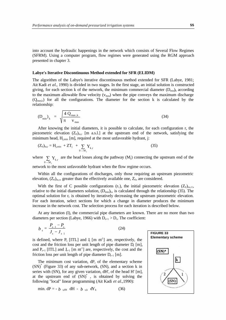
The minimum cost variation, dP, of the elementary scheme(SN)* (Figure 33) of any sub-network, (SN), and a section k inseries with (SN), for any given variation, dH', of the head H' [m],at the upstream end of (SN)* , is obtained by solving thefollowing "local" linear programming (Ait Kadi et al.,1990):
min. dP = - β s,SN dH - β s,k dYk (36)
FIGURE 33Elementary scheme
Pipe-size calculation56
subject to:
dH + dYk = dH’ (37)
where dH [m] and dYk [m] are, respectively, the variation of the head at the upstream end of(SN) and the variation of the friction loss in section k. The optimal solution of the equations(36) and (37) is:
dH = dH' and dYk
= 0 if β s,SN < β s,k (38)
dH = 0 and dYk
= dH' if β s,SN > β s,k (39)
Therefore, the minimum cost variation, dP, of (SN)* can be written as:
dP = - β * dH' with (40)
β * = min (β s,SN , β s,k) (41)
Hence, proceeding from any terminal section of the pipe network, the equation (40) can beused to determine the section that will vary at each iteration. Note that in this process (Figure33), β s,SN of the assembly of two sections in derivation is equal to:
β s,SN = β s,1 + β s,2 (42)
whereas, for two sections in series it is equal to:
β s,SN = min ( β s,1 , β s,2) (43)
It should be mentioned that in the case of a terminal section with a head in excess at itsdownstream end (Hj > Hj,min), the value of β s,SN which is used in the process is equal to zero aslong as the excess head prevails.
The magnitude of dHi,r, for each iteration i and configuration r, is determined as:
dHi,r = min (EHi, ∆Yi, ∆Zi) (44)
where:
EHi is the minimum value of the excess head prevailing in all the nodes where the head willchange;
∆Yi is the minimum value of (Yk,i - Y*) for those sections that change in diameter, with Yk,i
being the value of the head loss in the section k at iteration i, and Y* is, for this section, thevalue of the head loss corresponding to the largest diameter over its entire length if thesection has two diameters, or the next greater diameter if the section has only one diameter.Note that for those terminal sections with head in excess (H j > Hj,min), ∆Yi is equal to thevalue of this excess (Hj - Hj,min).
∆Zi is the difference between the upstream piezometric elevation, (Z0)i,r1 , at iteration i when theflow regime r1 occurs, and the piezometric elevation, Z0, effectively available at the upstreamend of the network.
The iterative process is continued until Z0 is reached, obtaining the optimal solution for theexamined configuration, r1. This solution is considered as the initial solution for the nextconfiguration (r2) and the iterative process is repeated. The process is continued until all thedischarge configurations, C, have been considered. Diameters of the sections can only increaseor remain constant for the previous analysed configurations to be satisfied. The final optimalsolution should satisfy all the examined discharge configurations.
Performance analysis of on-demand pressurized irrigation systems 57
A computer program for calculating the optimal pipe size of an irrigation network under bothseveral discharge configurations and in case of single flow regime has been developed(Lamaddalena, 1997) and integrated into the COPAM package. The ELIDM has been validatedusing the linear programming formulation extended for several flow regimes (Ben Abdellah,1995; Lamaddalena, 1997). The commercial computer package (LINDO) was adapted forcalculating the optimal solution for the irrigation network with linear programming.
Darcy's equation was used in ELIDM for calculating the friction slope J [m m-1] in the pipes:
J = 0.000857 (1 + 2γ D-0.5 ) 2 Q2 D-5 = u Q2 (45)
where γ is the roughness parameter of Bazin, expressed in m0.5. The other variables have beenalready defined in the text. In Table 4 the values of the roughness Bazin parameters for differenttypes of pipes are reported. They are compared with the values of the equivalent homogeneousroughness ε (mm). Information on the different types of pipes is reported in Annex 2.TABLE 4Bazin roughness parameter (γ) for different types of pipes
TYPE OF PIPEEquivalent
homogenousroughness
ε ( mm )
γ
( m0.5 )
1- Technically smooth tubes ( glass, brass, drawn copper, resin ) 0 ÷ 0.02 --2- Steel pipes
A ) Time degradable coverings- New pipes, varnished by centrifugation 0.05 --- Bitumened by immersion 0.1 ÷ 0.015 ≤ 0.06- In current duty with light rust 0.2 ÷ 0.4 0.10- With asphalt or tar applied by hands 0.5 ÷ 0.6 0.16- With diffused tubercolisation 1 ÷ 3 0.23
B ) Non degradable coverings- Cement applied by centrifugation 0.05 ÷ 0.15 ≤ 0.06
3- Welded sheet-pipes- In good conditions 0.2 ÷ 0.3 0.10- In current duty with crusting 0.4 ÷ 1.0 0.16
4- Nailed sheet-pipes- 1 line of longitudinal nails 0.3 ÷ 0.4 0.10- 2 lines of longitudinal nails 0.6 ÷ 0.7 0.16- Idem with crusting Till 3.0 0.30- 4-6 lines of longitudinal nails 2.0 0.23- 6 lines of longitudinal nails + 4 transversal 3.0 0.30- Idem with crusting Till 5.0 0.36
5- Cast iron pipes- With centrifuged-cemented covering 0.1 ≤ 0.06- New, covered internally with bitumen 0.15 0.06- New, not covered 0.2 ÷ 0.4 0.10- With light crusting 0.4 ÷ 1.0 0.16- In current duty, partially rusted 1.0 ÷ 2.0 0.23- strongly encrusted 3.0 ÷ 5.0 0.36
6- Cement-pipes- Asbestos cement 0.1 ≤ 0.06- New reinforced concrete, plaster perfectly smooth 0.1 ÷ 0.15 0.06
- Reinforced concrete with smooth plaster, in work for many years 2.0 0.23- Tunnels with cement plaster, depending on the degree of finish 2.0 ÷ 5.0 0.23 ÷ 0.36
The applicability of the ELIDM in the case of a network with SFR is presented in the nextsection.
Pipe-size calculation58
FIGURE 34Costs (106 ITL) of the network in the example, calculatedby using the ELP and the ELIDM for different sets of flowregimes
Applicability
In this section, the applicability ofthe Labye iterative discontinuousmethod has been verified throughthe linear programming formula-tion. Both the methods have beenapplied to a network under severalflow regimes.
The RGM presented in chapter3 was previously used forgenerating different sets ofrandom discharge configurations.These sets of configurations havebeen utilized for the calculation ofthe optimal diameters using theELP and ELIDM programs.
The difference in cost of thenetwork under study is shown inFigure 34. It is always less than2% because in the ELPformulation all the dischargeconfigurations are considered as a unique block and, thus, the exact solution is obtained. In theELIDM program the configurations are considered one by one, with the final solution for theconfiguration ri being the initial solution for the ri+1 configuration. Therefore, diameters of thesections can only increase or remain constant when the configurations change. For this reason,the order of the discharge configurations during the calculation has little effect on the optimalsolution.
The differences between the ELP and the ELIDM are small. When several dischargeconfigurations are considered, the latter method is preferred because it is more flexible and thecomputation time is very short (a few seconds for each discharge configuration). Furthermore,the computer software integrated in the COPAM package is user-friendly and allows thecalculation of networks up to 1000 nodes under more than 1000 flow regimes.
THE INFLUENCE OF THE PUMPING STATION ON THE PIPE SIZE COMPUTATION
The basic relationship between the pumping station at the upstream end of an irrigation systemand the pipe network is that the higher upstream pressure the lower the diameters of thenetwork, and vice versa. The other important relationship is that the higher the pressure thehigher the costs of the pumping station and the energy.
Through the optimization programs we can compute the variation of the network costs fordifferent upstream piezometric elevations “z”. On the other hand, the piezometric elevation canbe translated into energy and pumping station costs. The total cost for the irrigation system(network, pumping station and energy) is given by the sum of both costs. The total cost isrepresented by a curve having a minimum value corresponding to an optimal solution (Figure35). It is understood that all costs must be referred to the same life span and therefore must beactualized.
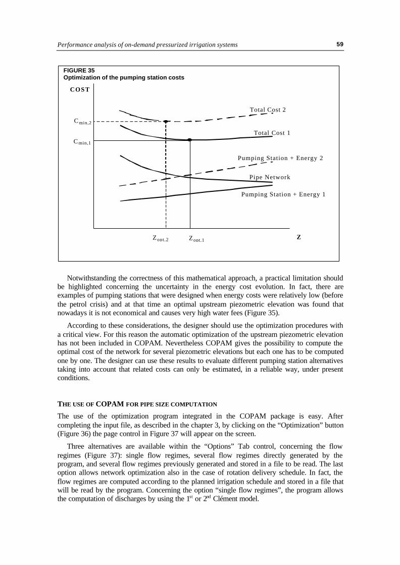
Performance analysis of on-demand pressurized irrigation systems 59
Notwithstanding the correctness of this mathematical approach, a practical limitation shouldbe highlighted concerning the uncertainty in the energy cost evolution. In fact, there areexamples of pumping stations that were designed when energy costs were relatively low (beforethe petrol crisis) and at that time an optimal upstream piezometric elevation was found thatnowadays it is not economical and causes very high water fees (Figure 35).
According to these considerations, the designer should use the optimization procedures witha critical view. For this reason the automatic optimization of the upstream piezometric elevationhas not been included in COPAM. Nevertheless COPAM gives the possibility to compute theoptimal cost of the network for several piezometric elevations but each one has to be computedone by one. The designer can use these results to evaluate different pumping station alternativestaking into account that related costs can only be estimated, in a reliable way, under presentconditions.
THE USE OF COPAM FOR PIPE SIZE COMPUTATION
The use of the optimization program integrated in the COPAM package is easy. Aftercompleting the input file, as described in the chapter 3, by clicking on the “Optimization” button(Figure 36) the page control in Figure 37 will appear on the screen.
Three alternatives are available within the “Options” Tab control, concerning the flowregimes (Figure 37): single flow regimes, several flow regimes directly generated by theprogram, and several flow regimes previously generated and stored in a file to be read. The lastoption allows network optimization also in the case of rotation delivery schedule. In fact, theflow regimes are computed according to the planned irrigation schedule and stored in a file thatwill be read by the program. Concerning the option “single flow regimes”, the program allowsthe computation of discharges by using the 1st or 2nd Clément model.
FIGURE 35Optimization of the pumping station costs
Zopt,2 Zopt,1
Pipe Network
Pumping Station + Energy 1
Pumping Station + Energy 2
Total Cost 1
Total Cost 2
COST
Z
C min,2
C min,1
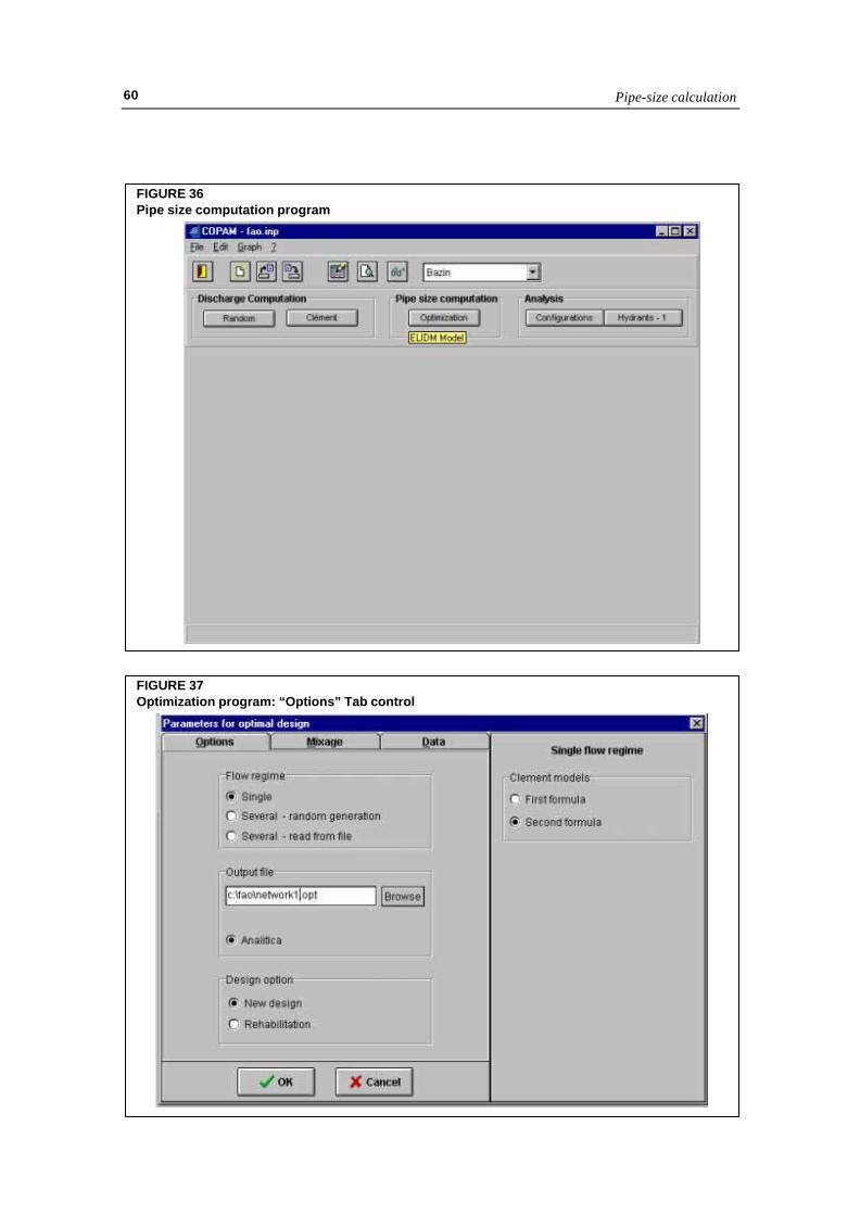
Pipe-size calculation60
FIGURE 36Pipe size computation program
FIGURE 37Optimization program: “Options” Tab control
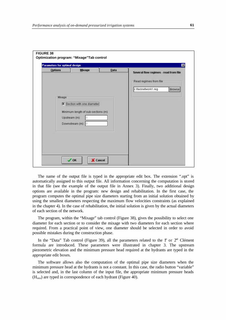
Performance analysis of on-demand pressurized irrigation systems 61
The name of the output file is typed in the appropriate edit box. The extension “.opt” isautomatically assigned to this output file. All information concerning the computation is storedin that file (see the example of the output file in Annex 3). Finally, two additional designoptions are available in the program: new design and rehabilitation. In the first case, theprogram computes the optimal pipe size diameters starting from an initial solution obtained byusing the smallest diameters respecting the maximum flow velocities constraints (as explainedin the chapter 4). In the case of rehabilitation, the initial solution is given by the actual diametersof each section of the network.
The program, within the “Mixage” tab control (Figure 38), gives the possibility to select onediameter for each section or to consider the mixage with two diameters for each section whererequired. From a practical point of view, one diameter should be selected in order to avoidpossible mistakes during the construction phase.
In the “Data” Tab control (Figure 39), all the parameters related to the 1st or 2nd Clémentformula are introduced. These parameters were illustrated in chapter 3. The upstreampiezometric elevation and the minimum pressure head required at the hydrants are typed in theappropriate edit boxes.
The software allows also the computation of the optimal pipe size diameters when theminimum pressure head at the hydrants is not a constant. In this case, the radio button “variable”is selected and, in the last column of the input file, the appropriate minimum pressure heads(Hmin) are typed in correspondence of each hydrant (Figure 40).
FIGURE 38Optimization program: “Mixage”Tab control
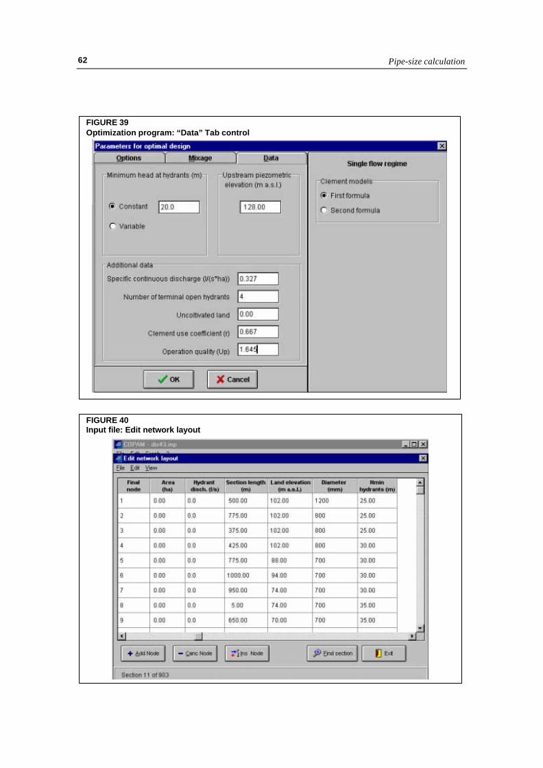
Pipe-size calculation62
FIGURE 39Optimization program: “Data” Tab control
FIGURE 40Input file: Edit network layout
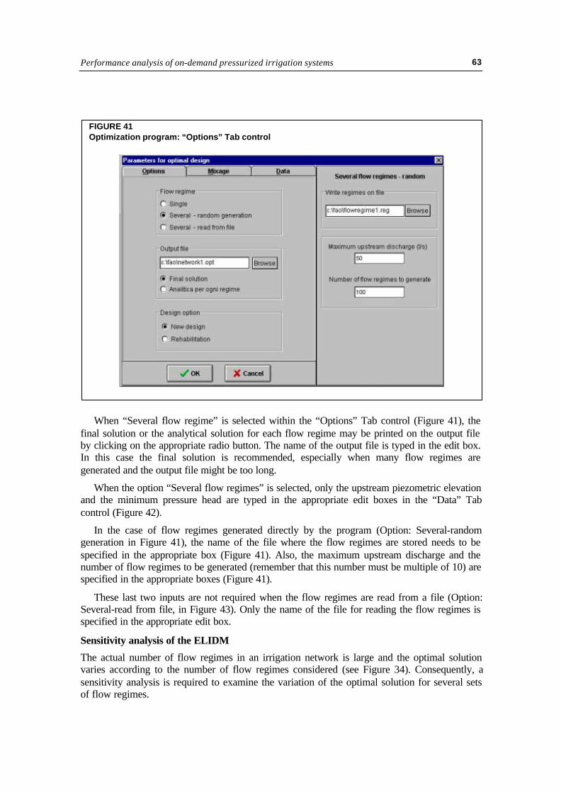
Performance analysis of on-demand pressurized irrigation systems 63
When “Several flow regime” is selected within the “Options” Tab control (Figure 41), thefinal solution or the analytical solution for each flow regime may be printed on the output fileby clicking on the appropriate radio button. The name of the output file is typed in the edit box.In this case the final solution is recommended, especially when many flow regimes aregenerated and the output file might be too long.
When the option “Several flow regimes” is selected, only the upstream piezometric elevationand the minimum pressure head are typed in the appropriate edit boxes in the “Data” Tabcontrol (Figure 42).
In the case of flow regimes generated directly by the program (Option: Several-randomgeneration in Figure 41), the name of the file where the flow regimes are stored needs to bespecified in the appropriate box (Figure 41). Also, the maximum upstream discharge and thenumber of flow regimes to be generated (remember that this number must be multiple of 10) arespecified in the appropriate boxes (Figure 41).
These last two inputs are not required when the flow regimes are read from a file (Option:Several-read from file, in Figure 43). Only the name of the file for reading the flow regimes isspecified in the appropriate edit box.
Sensitivity analysis of the ELIDM
The actual number of flow regimes in an irrigation network is large and the optimal solutionvaries according to the number of flow regimes considered (see Figure 34). Consequently, asensitivity analysis is required to examine the variation of the optimal solution for several setsof flow regimes.
FIGURE 41Optimization program: “Options” Tab control
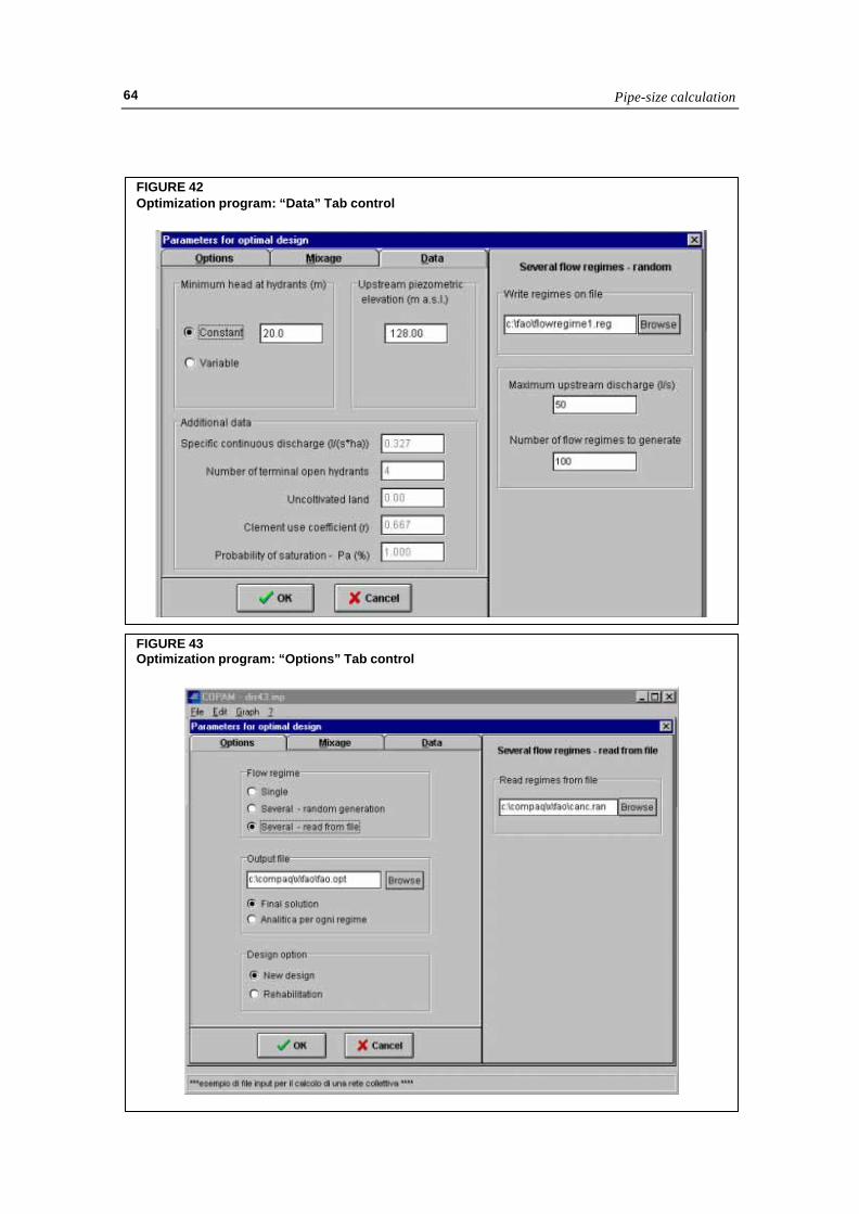
Pipe-size calculation64
FIGURE 42Optimization program: “Data” Tab control
FIGURE 43Optimization program: “Options” Tab control
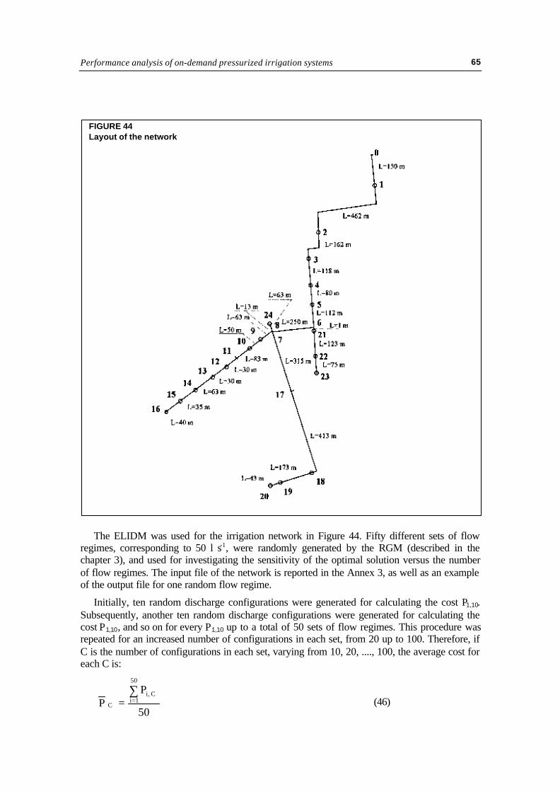
Performance analysis of on-demand pressurized irrigation systems 65
The ELIDM was used for the irrigation network in Figure 44. Fifty different sets of flowregimes, corresponding to 50 l s-1, were randomly generated by the RGM (described in thechapter 3), and used for investigating the sensitivity of the optimal solution versus the numberof flow regimes. The input file of the network is reported in the Annex 3, as well as an exampleof the output file for one random flow regime.
Initially, ten random discharge configurations were generated for calculating the cost P1,10.Subsequently, another ten random discharge configurations were generated for calculating thecost P1,10, and so on for every P1,10 up to a total of 50 sets of flow regimes. This procedure wasrepeated for an increased number of configurations in each set, from 20 up to 100. Therefore, ifC is the number of configurations in each set, varying from 10, 20, ...., 100, the average cost foreach C is:
PP
50C
i, Ci 1
50
= =∑
(46)
FIGURE 44Layout of the network
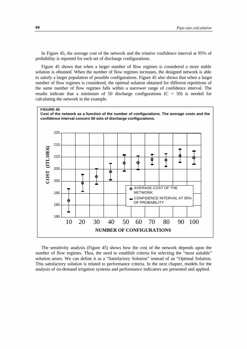
Pipe-size calculation66
In Figure 45, the average cost of the network and the relative confidence interval at 95% ofprobability is reported for each set of discharge configurations.
Figure 45 shows that when a larger number of flow regimes is considered a more stablesolution is obtained. When the number of flow regimes increases, the designed network is ableto satisfy a larger population of possible configurations. Figure 45 also shows that when a largernumber of flow regimes is considered, the optimal solution obtained for different repetitions ofthe same number of flow regimes falls within a narrower range of confidence interval. Theresults indicate that a minimum of 50 discharge configurations (C = 50) is needed forcalculating the network in the example.
The sensitivity analysis (Figure 45) shows how the cost of the network depends upon thenumber of flow regimes. Thus, the need to establish criteria for selecting the “most suitable”solution arises. We can define it as a “Satisfactory Solution” instead of an “Optimal Solution.This satisfactory solution is related to performance criteria. In the next chapter, models for theanalysis of on-demand irrigation systems and performance indicators are presented and applied.
10 20 30 40 50 60 70 80 90100
FIGURE 45Cost of the network as a function of the number of configurations. The average costs and theconfidence interval concern 50 sets of discharge configurations.
185
190
195
200
205
210
215
220
NUMBER OF CONFIGURATIONS
CO
ST (
ITL
10E
6)
AVERAGE COST OF THE NETWORK CONFIDENCE INTERVAL AT 95% OF PROBABILITY
10 20 30 40 50 60 70 80 90 100