Embed Size (px)
Citation preview
Modeling Flow Characteristics of a Low Specific-Speed
Centrifugal Pump with Different Volute Shapes
by
Susan Daly Wettermark
Submitted to the
Department of Mechanical Engineering
in Partial Fulfillment of the Requirements for the Degree of
Course 2: Bachelor of Science in Mechanical Engineering
at the
Massachusetts Institute of Technology
June 2019
© 2019 Massachusetts Institute of Technology. All rights reserved.
Signature of Author:
Department of Mechanical Engineering
May 16, 2019
Certified by:
Alexander Slocum
Walter M. May and A. Hazel May Professor of Mechanical Engineering
Thesis Supervisor
Accepted by:
Maria Yang
Professor of Mechanical Engineering
Undergraduate Officer

2
Modeling Flow Characteristics of a Low Specific-Speed
Centrifugal Pump with Different Volute Shapes
by
Susan Daly Wettermark
Submitted to the Department of Mechanical Engineering
on May 10, 2019 in Partial Fulfillment of the
Requirements for the Degree of
Course 2: Bachelor of Science in Mechanical Engineering
Abstract
A centrifugal pump is typically designed for a specific operating condition. The pump’s shape
and size are fine-tuned so that it can produce a specified output pressure and flow rate at the
maximum possible efficiency. When a pump begins operating off of its design flow rate, its
efficiency drops.
Pumping systems often involve dynamic demands. They may have a fluctuating flow rate
demand throughout the day, or the system may evolve and change size over time. In these cases,
pumps with a single operating point are inefficient and insufficient.
This thesis assesses the effects of changing a pump’s volute casing geometry on the volute’s
internal flow characteristics. All analysis is performed on a low-specific-speed, radial flow
centrifugal pump. 2D flow models from literature and CFD are analyzed and compared to
experimental data. With properly-chosen solution methods, a 2D CFD simulation is found to
match well with experimental results. Efficiency estimates and life-cycle cost changes due to
changing flow characteristics in the variable volute system are presented.
Thesis Supervisor: Alexander Slocum
Tile: Walter M. May and A. Hazel May Professor of Mechanical Engineering

3
Acknowledgements
Thank you to Hilary Johnson for being a fantastic mentor with open ears, for asking
thoughtful questions, and for inspiring me with your attitude towards what you do and your
work-life balance. Thank you to Prof. Alex Slocum for reminding me about the big picture and
the value of time. Thank you to Kevin Simon for providing guidance and thoughtful answers to
my simple questions. Thank you to Julia Cummings for working through the understanding of
pumps with me and helping me think critically about what we’re trying to accomplish. Thank
you to all of PERG lab for exemplifying openness, maturity, and excitement about the things you
do. Thank you to Max Kessler for constant support and motivation.

4
Table of Contents Abstract ......................................................................................................................................................... 2
Acknowledgements ....................................................................................................................................... 3
List of Figures ................................................................................................................................................................ 5
List of Tables ................................................................................................................................................................. 5
Naming Conventions ..................................................................................................................................................... 6
1. Background ............................................................................................................................................... 6
1.1 Centrifugal Pumps ............................................................................................................................................... 6
1.2 Pumping Systems with Changing Demand ......................................................................................................... 8
1.3 Changing Volute Geometry to Expand Efficient Flow Rates ............................................................................. 9
2. Pump-Design Methods and their relevance to changing volute shape ...................................................... 9
2.1 Volute-Impeller Matching ................................................................................................................................... 9
2.2 Specific Speed Analysis .................................................................................................................................... 11
2.3. CFD .................................................................................................................................................................. 11
2.4. Experiment ....................................................................................................................................................... 11
3. Models of flow through the volute .......................................................................................................... 12
3.1. General Assumptions ....................................................................................................................................... 12
3.2. Control Volume Analysis on Simplified Geometry ......................................................................................... 13
3.3. Iversen [15] ...................................................................................................................................................... 16
3.4. Lorett [16] ........................................................................................................................................................ 18
4. Dimensions used for analysis .................................................................................................................. 20
5. CFD Setup and Assumptions .................................................................................................................. 23
Geometry ................................................................................................................................................................. 23
Meshing ................................................................................................................................................................... 24
CFD Setup and Solution .......................................................................................................................................... 24
Data Processing ....................................................................................................................................................... 29
6. Results ..................................................................................................................................................... 29
6.1. Specific Speed Analysis ................................................................................................................................... 29
6.2. Volute-Impeller Matching Analysis ................................................................................................................. 30
6.3. Analysis of CFD Model ................................................................................................................................... 31
6.4. Comparison of Models for Pressure Distribution in Volute ............................................................................. 32
6.5 Effect of Surface Roughness on Volute Pressure Balance and Efficiency ........................................................ 34
6.6. Life-cycle Cost Analysis of Efficiency and Pressure ....................................................................................... 35
7. Conclusions ............................................................................................................................................. 38
8. References ............................................................................................................................................... 39
9. Appendix ................................................................................................................................................. 40
Additional Volute Parameters ................................................................................................................................. 40
MATLAB code for analyzing CFD data ................................................................................................................. 42
MATLAB code for calculating model in section 3.2 from impeller outlet to throat ............................................... 49

5
List of Figures Figure 1. Centrifugal Pump Cross-Section ................................................................................................... 7
Figure 2. Pump Characteristic Curve ........................................................................................................... 7
Figure 3. Volute and Impeller Characteristic Curve Relationsips .............................................................. 10
Figure 4. Zero-Flow Impeller Head Coefficient Relationship .................................................................... 11
Figure 5. Unwrapped linear volute model for control volume analysis ..................................................... 13
Figure 6. Discretized volute segment used for control volume analysis .................................................... 17
Figure 7. CAD Geometries and dimensions used for analysis ................................................................... 21
Figure 8. Five different volute sizes analyzed ............................................................................................ 22
Figure 9. Mesh used for 2D CFD analysis of centrifugal pump. ................................................................ 24
Figure 10. Contour plots for 2D centrifugal pump simulation. .................................................................. 26
Figure 11. Comparison of k-ω and k-ε solution methods for a 2D centrifugal pump model ..................... 27
Figure 12. Variation of 2D CFD solution methods compared with experimental data [7] for centrifugal
pump ........................................................................................................................................................... 27
Figure 13. Total Dynamic Head vs Flow Rate for centrifugal pump 2D CFD model vs experiment ........ 28
Figure 14. Convergence of solution for 2D pump simulation. .................................................................. 28
Figure 15. Characteristics of several different volute sizes compared with the characteristic of a single
impeller shape ............................................................................................................................................. 30
Figure 16. CFD-simulated surface plots for the total pressure in the volute area of a 2D centrifugal pump
model. ......................................................................................................................................................... 31
Figure 17. CFD-simulated results for the average pressure imbalance on opposite sides of the impeller. 32
Figure 18. Comparison of three models for the impeller’s circumferential static pressure distribution .... 33
Figure 19. Comparison of two models for the change in pressure within the volute. ................................ 34
Figure 20. Comparison of flow characteristics for a centrifugal pump with different surface roughness
values in the volute. ................................................................................................................................... 35
Figure 21. Hydraulic efficiency of the volute component of a 2D centrifugal pump simulation ............... 36
List of Tables Table 1: Assumptions for all analytical models .......................................................................................... 12
Table 2: Assumptions of the linear expanding diffuser model ................................................................... 14
Table 3: Assumptions of the Iversen model ................................................................................................ 16
Table 4: Assumptions for the Lorett Model ................................................................................................ 18
Table 5. Physical Dimensions of Volutes and Impeller used for Analysis ................................................. 21
Table 6.1 Flow-rate-specific parameters used for analysis. ........................................................................ 22
Table 6.2-6.5 - Additional Volute Parameters…………………...………………………………..Appendix
Table 7 – Assumptions made in 2D analysis of centrifugal pump ............................................................. 25
Table 8 – Setup and solution methods used in 2D CFD simulation of centrifugal pump ........................... 25
Table 9 Minimum and Maximum Flow Rates for Low Specific-Speed Pump ........................................... 30
Table 10 Comparison of Experiment and Characteristic Curve Best-Efficiency Points ............................ 31
Table 11 Comparison of Models for hydraulic efficiency and average impeller pressure imbalance ........ 33
6
Naming Conventions The remainder of this thesis will use the naming conventions defined below, unless otherwise specified.
The naming conventions are based off of those used in Gülich’s Centrifugal Pumps [1].
Geometric
Parameters
Kinematic Parameters Material and Surface
Properties
Subscripts
𝐷 Diameter 𝛼 Angle of velocity
entry into volute
𝜌 Density of water 1 Impeller blade leading
edge
𝑟 Radius 𝜃 Angular position
around volute 𝜇 Kinematic
viscosity of water 2 Impeller blade trailing
edge, impeller outlet
𝑎 Volute height 𝑐 Absolute velocity
magnitude 𝑓 Volute wall
friction factor 3 Volute cutwater, at
base circle
4 Volute outlet
𝑏 Volute depth 𝑤 Relative velocity
magnitude
𝑚 Meridional/radial
component
𝛽 Blade outlet
angle 𝜂 Hydraulic
efficiency
𝑢 Tangential component
𝜙 Volute growth
angle
𝑤 water
𝐴 area 𝑜𝑝𝑡 Operating at best
efficiency point
I,II,III, IV,V
Test volute geometries
1. Background
1.1 Centrifugal Pumps Pumping systems enable modern life. They facilitate manufacturing processes by providing pressure
for machines and fluid for cooling. They transport domestic water and sewage. They facilitate
desalination of seawater on ships and remove water from underground during mining operations [2]. They
also move slurries of fluid for the oil and gas industry [3]. The European Commission estimated that of
the electric motor energy used worldwide, 20% is used to power pumps. Factories may use as much as
50% of their electricity on pumping systems [4].
The centrifugal pump is one of the most common pump types. Centrifugal pumps induce flow
through piping networks by first adding kinetic energy to a fluid and then converting that kinetic energy
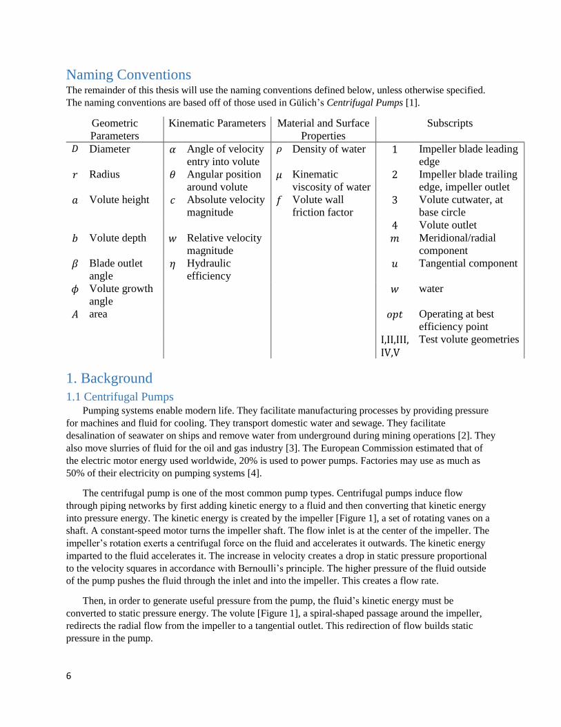
into pressure energy. The kinetic energy is created by the impeller [Figure 1], a set of rotating vanes on a
shaft. A constant-speed motor turns the impeller shaft. The flow inlet is at the center of the impeller. The
impeller’s rotation exerts a centrifugal force on the fluid and accelerates it outwards. The kinetic energy
imparted to the fluid accelerates it. The increase in velocity creates a drop in static pressure proportional
to the velocity squares in accordance with Bernoulli’s principle. The higher pressure of the fluid outside
of the pump pushes the fluid through the inlet and into the impeller. This creates a flow rate.
Then, in order to generate useful pressure from the pump, the fluid’s kinetic energy must be
converted to static pressure energy. The volute [Figure 1], a spiral-shaped passage around the impeller,
redirects the radial flow from the impeller to a tangential outlet. This redirection of flow builds static
pressure in the pump.
7
Figure 1. Cross-sectional view of a typical centrifugal pump design. The flow enters
through the inlet at the center of the blades, travels radially outward along the blade, and
flows around the spiral volute before exiting. The base circle radius is the distance from
the impeller center to the cutwater, where the volute spiral begins.
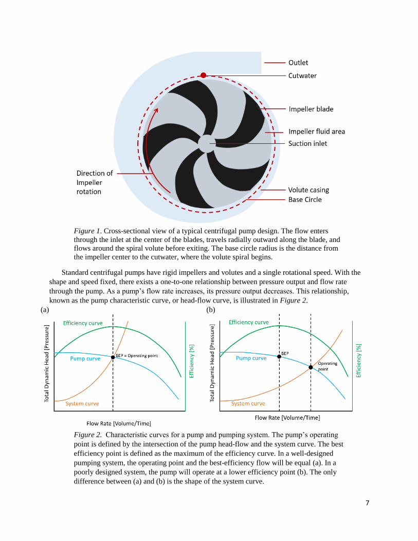
Standard centrifugal pumps have rigid impellers and volutes and a single rotational speed. With the
shape and speed fixed, there exists a one-to-one relationship between pressure output and flow rate
through the pump. As a pump’s flow rate increases, its pressure output decreases. This relationship,
known as the pump characteristic curve, or head-flow curve, is illustrated in Figure 2.
(a) (b)
Figure 2. Characteristic curves for a pump and pumping system. The pump’s operating
point is defined by the intersection of the pump head-flow and the system curve. The best
efficiency point is defined as the maximum of the efficiency curve. In a well-designed
pumping system, the operating point and the best-efficiency flow will be equal (a). In a
poorly designed system, the pump will operate at a lower efficiency point (b). The only
difference between (a) and (b) is the shape of the system curve.

8
The pump can operate at any point along the head-flow. Its operating point is determined by the
characteristics of the system that it supplies. The system curve is found through system testing and
modeling. It is either flat or positively sloped – most often a parabolic shape - because providing
additional flow to a system requires additional pressure to overcome friction and energy losses.
The goal in selecting a pump is to choose a pump that has a best efficiency point at the intersection of
its head-flow curve and the system curve. Designers will make their best estimate of the system curve
based on the pressure requirements of the system’s components. However, engineering models of fluid
system are never perfectly precise. Because there is uncertainty in determining the system curve,
engineers will often add a safety factor to their calculations to ensure that they don’t get a pump that lacks
power to do the required job. As a result, an estimated 75% of pumps are oversized [4]. A pump owner
logically prefers a pump that is oversized and slightly less efficient rather than one that lacks power to
complete the required task.
1.2 Pumping Systems with Changing Demand Oversized pumps may also be intentionally purchased to handle an unsteady demand for flow rate.
Supply-controlled systems, such as storm-water drainage, must handle whatever upstream flow is
provided to them. Demand-controlled systems, such as municipal drinking water supply, must be able to
adapt in real time to the water demands from the end users [4]. The system must be designed to
accommodate the maximum flow requirement, even if it is only needed a small percentage of the time.
This is often achieved by using pumps staged in parallel, such that additional pumps can be turned on in
times of high demand. Elevated storage tanks may also be used to provide extra flow. The extra pumps
and storage features add complexity and maintenance costs to the system, and these features sit
underutilized much of the time.
In the opposite situation, when a pump has a flow rate in excess of what the system requires, the
excess flow is typically throttled using pressure-actuated valves. The throttled fluid’s energy is therefore
lost, decreasing the pumping system’s efficiency [5].
Systems with unsteady flow demand may benefit from pumps that can provide a variable flow rate,
and industry has responded with various ways to change a pump’s characteristic curve. For slowly-
changing systems, trimming and shaping pumps’ impeller blades or volute tongues can modify
performance [6]. Trimming impeller blades, or swapping out impeller blades, can change the flow rate for
a system that remains stable for long durations, but it cannot solve the issue of rapidly-changing flow
demand. Replaceable hydraulic parts [7], such as diffusers or impeller modifiers, can provide different
flows rate without making permanent changes to the pump, but this change cannot be made in real time.
The most refined method for changing the flow rate in real time is using a variable-frequency
motor drive (VFD). VFDs control the speed of the impeller to change the flow rate, reducing energy
usage as much as 50% for off-design flows [5], depending on the system. However, there are limitations
to VFDs that make them impractical to use in some applications.
1. Operating pumps impellers at lower speeds can cause clogging due to debris or sedimentation
settling in the pump.
2. When changing the motor frequency, it is possible to accidentally excite one of the pump’s
natural frequencies, causing vibration and damage. Because VFD’s are often retroactively added
to pumps, the pump design may not account for the effects of being driven at different speeds.

9
3. VFD’s shift the pump characteristic curve down, so both flow rate and pressure output will
decrease when a lower speed is used, and vice versa. In some cases it may be detrimental to have
pressure change positively with flow.
4. VFD’s are expensive and require familiarity with electronics to implement, which may be
difficult for smaller pump systems or systems designed to be low-maintenance.
1.3 Changing Volute Geometry to Expand Efficient Flow Rates A new approach to varying a pump’s flow rate is dynamically changing the geometry of the pump’s
volute casing during operation. The design of a system to accomplish this is the topic of Hilary Johnson’s
doctoral research [7]. The present thesis investigates aspects of this idea in support of the doctoral
research. The goal of changing the volute shape is to shift the head-flow curve such that the best-
efficiency point also shifts and aligns with the desired flow rate.
A changeable geometry can address the main issues faced by VFD’s:
1. By retaining the original impeller speed, it may be easier to flush out debris than with a VFD.
2. The changing volute’s shape could be designed in such a way that it changes the pump’s natural
frequency and prevents excitations at specific flow rates.
3. An adjustable-geometry volute may be able to provide an off-design flow rate with an output
head closer to the original BEP head, unlike a VFD, because the impeller speed can remain
constant.
4. An adjustable-geometry volute must be able to provide lifetime cost savings high enough to
justify the cost of a more complicated pump design. However, they have the potential to simplify
pumping systems by requiring fewer components.
Previous studies have found that the head-flow curve can be shifted by changing the volute shape
with a fixed impeller shape [8,9]. However, the long-term effects of operating a fixed impeller with
different volute shapes are not well studied. A primary concern is an imbalance of pressure around the
impeller. Volutes are designed to produce an equal pressure around the impeller periphery at BEP. It is
unknown whether creating multiple BEPs with multiple volute shapes would maintain the pressure
balance. Another concern is how using different materials for a changeable volute design, would affect
the flow and pressure distribution, since many engineering materials have a lower surface roughness than
the cast-iron of most volutes. The remainder of this thesis will address these uncertainties and recommend
analytical models to predict their effects.
2. Pump-Design Methods and their relevance to changing volute shape
2.1 Volute-Impeller Matching Both the impeller and the volute have a characteristic curve that relates the head that they supply
to the flow that they supply. Impellers increase velocity and decrease static pressure, so the impeller
characteristic curve is negatively sloped. Volutes reduce kinetic energy and build pressure, so their curve
is have a positively-sloped. The two curves’ intersection marks the volute-impeller combination’s best-
efficiency point at a given rotational speed. This relationship is illustrated by Figure 3.
The equations in Figure 3 are dimensionless. To apply them to a specific pump in Section 6 of
this text, the head coefficient and flow ratio are multiplied by 𝜂ℎ∗𝑢2
2
𝑔 and 𝑢2, respectively. Introducing units
to the confidents allows the explicit prediction of head and flow rate at the curve intersection expressed in
units. Additionally, in Figure 3 the throat width and the throat height are equal, B. The volutes analyzed
in Section 6 do not have an equal height and width at the outlet, so the relationships in Figure 3 were

10
modified by the author. 𝑎3 and 𝑏3 are used instead of B for the volute throat area, and 𝐷ℎ,3 is used for the
hydraulic diameter instead of D. The modified relationships are given in equations 2.1 and 2.2
Figure 3. Reproduced from Worster [10]. The chart illustrates the non-dimensional head
coefficients for a volute and an impeller, based on their geometry as well as the pump’s
operating speed and flow rate. The intersection of the dotted volute characteristic curve
and the solid impeller characteristic curve represent the best-efficiency point for this
combination. At other flow rates, the impeller-volute combination is mismatched, and
reduced efficiency will be observed.
𝐻𝑖𝑚𝑝𝑒𝑙𝑙𝑒𝑟 = 𝜂ℎ∗𝑢2
2
𝑔(ℎ0 −
𝑄
𝜋∗𝑢2∗𝐷2∗𝑏2∗tan𝛽) (2.1)
𝐻𝑣𝑜𝑙𝑢𝑡𝑒 = 𝜂ℎ∗𝑢2
𝑔(
2𝑄∗𝐷ℎ,3
𝑎3∗𝑏3∗𝐷2∗ln(1+2𝐷ℎ,3𝐷2
)) (2.2)
The hydraulic efficiency 𝜂ℎ is not known until experimentally verified. However, it only serves to
scale the curves in these relationships and does not affect the intersection flow rate. The BEP flow rate of
a volute-impeller combination will be estimated and compared with experimental results. It will then be
used to predict the BEP flow of the impeller with different volute geometries
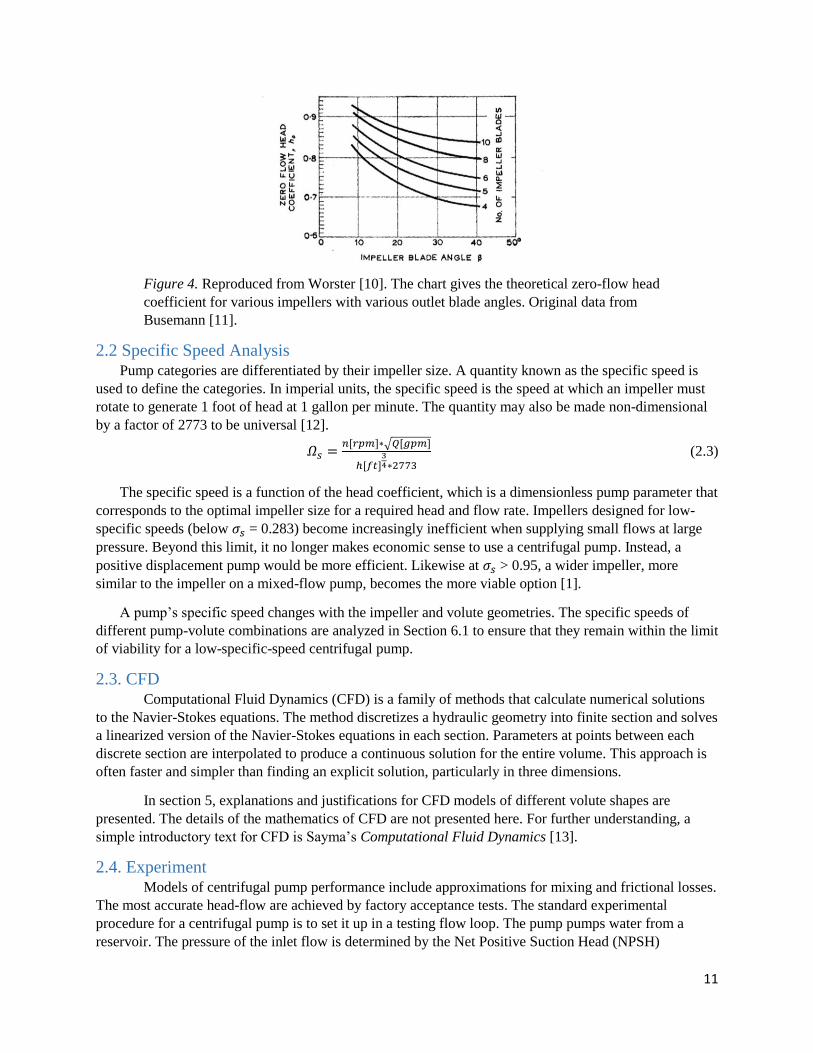
The impeller’s zero-flow head coefficient, ℎ0, will be estimated using Figure 4 [9,10].
11
Figure 4. Reproduced from Worster [10]. The chart gives the theoretical zero-flow head
coefficient for various impellers with various outlet blade angles. Original data from
Busemann [11].
2.2 Specific Speed Analysis Pump categories are differentiated by their impeller size. A quantity known as the specific speed is
used to define the categories. In imperial units, the specific speed is the speed at which an impeller must
rotate to generate 1 foot of head at 1 gallon per minute. The quantity may also be made non-dimensional
by a factor of 2773 to be universal [12].
𝛺𝑠 =𝑛[𝑟𝑝𝑚]∗√𝑄[𝑔𝑝𝑚]
ℎ[𝑓𝑡]34∗2773
(2.3)
The specific speed is a function of the head coefficient, which is a dimensionless pump parameter that
corresponds to the optimal impeller size for a required head and flow rate. Impellers designed for low-
specific speeds (below 𝜎𝑠 = 0.283) become increasingly inefficient when supplying small flows at large
pressure. Beyond this limit, it no longer makes economic sense to use a centrifugal pump. Instead, a
positive displacement pump would be more efficient. Likewise at 𝜎𝑠 > 0.95, a wider impeller, more
similar to the impeller on a mixed-flow pump, becomes the more viable option [1].
A pump’s specific speed changes with the impeller and volute geometries. The specific speeds of
different pump-volute combinations are analyzed in Section 6.1 to ensure that they remain within the limit
of viability for a low-specific-speed centrifugal pump.
2.3. CFD Computational Fluid Dynamics (CFD) is a family of methods that calculate numerical solutions
to the Navier-Stokes equations. The method discretizes a hydraulic geometry into finite section and solves
a linearized version of the Navier-Stokes equations in each section. Parameters at points between each
discrete section are interpolated to produce a continuous solution for the entire volume. This approach is
often faster and simpler than finding an explicit solution, particularly in three dimensions.
In section 5, explanations and justifications for CFD models of different volute shapes are
presented. The details of the mathematics of CFD are not presented here. For further understanding, a
simple introductory text for CFD is Sayma’s Computational Fluid Dynamics [13].
2.4. Experiment Models of centrifugal pump performance include approximations for mixing and frictional losses.
The most accurate head-flow are achieved by factory acceptance tests. The standard experimental
procedure for a centrifugal pump is to set it up in a testing flow loop. The pump pumps water from a
reservoir. The pressure of the inlet flow is determined by the Net Positive Suction Head (NPSH)

12
requirements of the pump. The system curve is determined by a control valve in the flow loop. Opening
and closing the valve changes the pressure requirement for providing flow to the system [1]. The flow
from the system is then returned to the reservoir. A flow-gauge and a pressure-gauge are connected on the
discharge side of the pump. A series of tests are run with the control valve in different positions. The
pump’s output flow and pressure are recorded for each condition.
3. Models of flow through the volute In designing an adaptable-geometry volute casing, it is essential to understand the patterns of
flow through a volute. Why does the pressure and velocity change in the way that it does between the
inlet and the outlet? What happens to the pressure and velocity inside the volute before it exits the pump?
It is useful to validate quick methods to predict velocity and pressure behaviors for assessing the
viability of new volute designs. Three models are presented here as ways to approximate the flow
behavior in the volute analytically. They begin with an over-simplified model to understand the basic
physics of how flow changes in a diffuser from a uniform-flow inlet to a uniform-flow outlet. The second
and third models are taken from literature and present estimations for the flow characteristics of a non-
uniform-flow inlet to the volute.
3.1. General Assumptions
Table 1 applies to all models presented. Model-specific assumptions are given in the subsequent sections.
Table 1: Assumptions for all analytical models
Assumption Affected
Variable
Reasoning
Incompressible Flow ρ Water is in the liquid phase for all operating points of the pump.
Within the liquid phase, the density of water changes by less
than 0.03% per degree of temperature change in this region, and
by less than 0.02% per change in pressure in foot of head [14].
1. Constant velocity
magnitude at
volute outlet
2. Velocity outlet
angle normal to
outlet face
3. Constant pressure
along outlet
𝑐3(𝑦) =𝑐𝑜𝑛𝑠𝑡.
𝛼3 = 0
𝑃3 = 𝑐𝑜𝑛𝑠𝑡.
It is assumed that the flow is fully-developed and uniform and
that there is no no-slip condition at the walls of the outlet.
Because the average velocity and pressure out of the pump
outlet are most important to know, it is assumed that the
uniform pressure in the model is representative of the average in
a real pump.
Gravitational forces
are negligible
- Centrifugal forces are the dominant forces that cause flow
acceleration in a centrifugal pump.
Change in head due to elevation changes in the pump are also
negligible as the hydraulic area only has a 5.6” diameter.
Wall shear stresses
and viscous forces
are negligible
- Reynolds number is high (106 – 107) for pump flows [Table 6.1
Flow-rate-specific parameters used for analysis.]
Meridional volute
inlet velocity is
calculated based on
the impeller surface
area
cm The impeller and volute must satisfy continuity at all times.
Therefore, the average meridional velocity out of the impeller
must create a known average inlet flow to the volute. Since the
effects of the widening flow area at the volute (b3 > b2) are
unknown, cm,2 is the best estimation of meridional velocity.
13
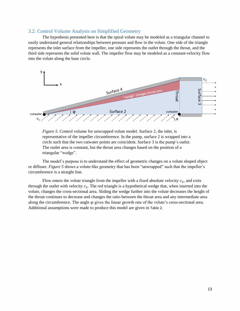
3.2. Control Volume Analysis on Simplified Geometry The hypothesis presented here is that the spiral volute may be modeled as a triangular channel to
easily understand general relationships between pressure and flow in the volute. One side of the triangle
represents the inlet surface from the impeller, one side represents the outlet through the throat, and the
third side represents the solid volute wall. The impeller flow may be modeled as a constant-velocity flow
into the volute along the base circle.
Figure 5. Control volume for unwrapped volute model. Surface 2, the inlet, is
representative of the impeller circumference. In the pump, surface 2 is wrapped into a
circle such that the two cutwater points are coincident. Surface 3 is the pump’s outlet.
The outlet area is constant, but the throat area changes based on the position of a
triangular “wedge”.
The model’s purpose is to understand the effect of geometric changes on a volute shaped object
or diffuser. Figure 5 shows a volute-like geometry that has been “unwrapped” such that the impeller’s
circumference is a straight line.
Flow enters the volute triangle from the impeller with a fixed absolute velocity 𝑐2, and exits
through the outlet with velocity 𝑐3. The red triangle is a hypothetical wedge that, when inserted into the
volute, changes the cross-sectional area. Sliding the wedge further into the volute decreases the height of
the throat continues to decrease and changes the ratio between the throat area and any intermediate area
along the circumference. The angle 𝜑 gives the linear growth rate of the volute’s cross-sectional area.
Additional assumptions were made to produce this model are given in Table 2.

14
Table 2: Assumptions of the linear unwrapped volute model
Assumption Affected Variable Reasoning Triangular volute
section 𝜑 = atan (
𝑎3
𝜋𝐷)
The linear section can be considered representative of the
constant-velocity volute design model, where flow rate and
velocity increase linearly around the volute’s circumference.
Width of volute wall
(Surface 4 in Figure
5) equals throat
width
b4 = b3 The volute shape has a corner radius and is not perfectly
rectangular in reality. For the purposes of this linear model, the
volute area will be approximated as its height multiplied by its
width, b3, because the changes in flow due to complex geometries
cannot be captured in a simple control volume analysis.
1. Constant velocity
magnitude volute
inlet
2. Constant velocity
angle along volute
inlet
3. Constant pressure
along volute inlet
𝑐2(𝑥) = 𝑐𝑜𝑛𝑠𝑡𝑎𝑛𝑡
𝛼 = 𝑐𝑜𝑛𝑠𝑡𝑎𝑛𝑡
𝑃2 = 𝑐𝑜𝑛𝑠𝑡𝑎𝑛𝑡
Volutes are designed to produce nearly-uniform velocity around
the impeller circumference. In reality, due to the pressure
imbalance between the impeller blade’s leading and trailing edges,
the velocity profile is not uniform at any instant. However, due to
the impeller’s rapid rotation, the time-averaged velocity around
the impeller circumference is assumed constant as a first-order
approximation.
In the unwrapped volute shape, there is no rotating impeller to
provide the flow. It is assumed that the flow comes from some
uniformly pressurized source as it enters the volute. This is a key
assumption and the model can assess its validity.
Pressure changes
linearly along
surface 4
𝑃4 = 𝑃2 + 𝑎𝑃3
𝑃2
Because the pressure at the cutwater is equal to the volute inlet
pressure and the pressure at the outlet is a different pressure, there
must be some change in pressure along the volute wall surface. As
a simple approximation, this relationship is assumed to be linear.
The normal vectors point in the direction out of the control surface.
𝑛2 = [0
−1] (3.2.1)
𝑛3 = [10] (3.2.2)
𝑛4 = [−sin𝜑cos𝜑
] (3.2.3)
First, the control volume can be modeled by continuity. This represents the volumetric flow rate assuming
no variation in flow across the volute’s width.
𝑉𝑖�� = 𝑉𝑜𝑢𝑡 (3.2.4)
𝐴𝑖𝑛 ∗ 𝑣𝑖𝑛 ∙ �� = 𝐴𝑜𝑢𝑡 ∗ 𝑣𝑜𝑢𝑡 ∗ �� (3.2.5)
𝜋 ∗ 𝐷2 ∗ 𝑏2 ∗ 𝑐2 ∗ 𝑛2 = 𝑎3 ∗ 𝑏3 ∗ 𝑐3 ∗ 𝑛3 (3.2.6)
Since the flow rate of the pump is known, the volumetric flow rate 𝑉 can be equated with a known 𝑄.
Using this relation, the magnitude of the velocity at the volute inlet and volute outlet are given by:
𝑐2 =𝑄
𝜋∗𝐷2∗𝑏2 (3.2.7)
𝑐𝑡ℎ𝑟𝑜𝑎𝑡 =𝑄
𝑎3∗𝑏3 (3.2.8)

15
𝑐3 =𝑄
𝜋𝑅𝑜𝑢𝑡𝑙𝑒𝑡 2 (3.2.9)
The momentum conservation principle relates the velocities to the pressures on each control volume wall. 𝑑��
𝑑𝑡= ∑𝐹𝐶𝑉
(3.2.10)
The time rate of change of momentum is expressed as:
𝑑��
𝑑𝑡= ∭
𝛿
𝛿𝑡𝜌𝑐
𝐶𝑉𝑑𝑉 + ∬ 𝜌𝑐 (𝑐 𝑏 ∙ ��)𝑑𝐴 +
𝐶𝑆 ∬ 𝜌𝑐 (𝑐 𝑟 ∙ ��)𝑑𝐴 𝐶𝑆
(3.2.11)
Where:
𝐿 = momentum vector
𝑐 𝑏 = velocity of control surface ( = 0 in this case_
𝑐 𝑟= fluid velocity relative to control surface ( = 𝑐 in this case)
The first term disappears since steady flow is assumed (𝛿𝑐
𝛿𝑡= 0) and the second term disappears
since the control volume is stationary (𝑐 𝑏 = 0). Therefore, only the third term remains. The third term can
then be expanded to include each of the three control surfaces shown in Figure 5.
𝑑��
𝑑𝑡= −∫ 𝜌𝑐2 (𝑐2 ∙ 𝑛2)𝑑𝑥
𝜋𝐷2
0− ∫ 𝜌𝑐3 (𝑐3(𝑦) ∙ 𝑛3)𝑑𝑦
𝑎3
0− ∫ 𝜌𝑐4(𝑥) (𝑐4(𝑥) ∙ 𝑛4)
𝑑𝑥
cos𝜃
𝜋𝐷2
0 (3.2.12)
The third term disappears since wall 4 has a no-slip boundary condition, so the velocity 𝑐4(𝑥) must be equal to zero along surface 4. The remaining terms are easily solved if constant velocity is
assumed at the inlet and outlet.
The inlet velocity is assumed constant along x:
𝑐2 = [|𝑐2|cos𝛼|𝑐2| sin 𝛼
] (3.2.13)
And the outlet velocity is constant along y:
𝑐3 = [|𝑐3|0
] (3.2.14)
Plugging in the expressions for the velocity and normal vectors in terms of Q and integrating yields the
following expression:
𝑑��
𝑑𝑡= 𝜌 [
𝑄2𝑎3 cot𝛼
𝜋2𝐷22𝑏2
−𝜋𝐷2𝑄
2
𝑎32𝑏3
𝑄2𝑎3
𝜋2𝐷22𝑏2
] (3.2.15)
Next, the expression for body forces acting on the fluid is:
∑𝐹𝐶𝑉 = ∯ −𝑝
𝐶𝑆�� 𝑑𝐴 + ∭ 𝜌 𝑔 𝑑𝑉
𝐶𝑉+ 𝐹𝑣𝑖𝑠𝑐𝑜𝑢𝑠 (3.2.16)
It is standard practice to neglect gravitational forces in pump modeling, as they are small relative
to the pressure forces and the direction of gravity is not constant relative to the direction of flow.
Therefore, the second term is neglected. Viscous terms may be modeled as part of the Reynolds stresses
for turbulent flow. For this model, they are neglected. Expanding the first term in the force equation for
the control surface yields:

16
∑𝐹𝐶𝑉 = −∫ 𝑏2𝑝2𝑛2𝑑𝑥
𝜋𝐷
0− ∫ 𝑏3𝑝3𝑛3𝑑𝑦
𝑎3
0− ∫ 𝑏3𝑝4(𝑥)𝑛4
𝑑𝑥
cos𝜑
𝜋𝐷
0 (3.2.17)
Where 𝑝4(𝑥) = 𝑝2 + (𝑝3 − 𝑝2)𝑥
𝜋𝐷 (3.2.18)
It is assumed that the pressure changes linearly along surface 4.
Therefore, these are the closed form solutions for the pressures at the volute inlet and at the throat:
𝑝2 =𝜌𝑄2(2𝑎3
4𝑏3 cos𝜑 sin𝛼+𝐷24𝑏2𝜋
4 cos𝜑 sin𝛼−𝜋𝐷2𝑎33𝑏3 cos𝜑 cos𝛼−𝜋𝐷2𝑎3
3𝑏3 sin𝜑 sin𝛼)
𝜋3𝐷23𝑎3
2𝑏2𝑏3 sin𝛼∗(𝑎3𝑏3 cos𝜑−2𝑎3𝑏2 cos𝜑+𝜋𝐷2𝑏2 sin𝜑) (3.2.19)
𝑝𝑡ℎ𝑟𝑜𝑎𝑡 = 𝜌𝑄2(2𝜋3𝐷2
3𝑏22 cos𝜑 sin𝛼+𝑎3
3𝑏32 cos𝜑 cos𝛼+𝑎3
3𝑏32 sin𝜑 sin𝛼−2𝑎3
3𝑏2𝑏3)
𝜋2𝐷22𝑎3
2𝑏2𝑏32 sin𝛼∗(𝑎3𝑏3 cos𝜑−2𝑎3𝑏2 cos𝜑+𝜋𝐷2𝑏2 sin𝜑)
(3.2.20)
The short length between the throat and the volute outlet is modeled as a linear diffuser. In this
area, the pressure changes with the change in velocity. The change in pressure between the throat and the
outlet is therefore given by:
𝑝𝑡ℎ𝑟𝑜𝑎𝑡 = 𝑝3 +𝑣3
2
2𝑔−
𝑣𝑡ℎ𝑟𝑜𝑎𝑡2
2𝑔 (3.2.21)
The total change in pressure across the system is given by
𝛥𝑝 = 𝑝𝑡ℎ𝑟𝑜𝑎𝑡 − 𝑝2 (3.2.22)
The results of this model’s implementation are presented in Section 6.4. The variable meanings
are given in Naming Conventions and their explicit values are defined in Section 4. The MATLAB code
used to calculate equations 3.2.19 and 3.2.20 is given in the appendix.
3.3. Iversen [15] “Volute Pressure Distribution, Radial Force on the Impeller, and Volute Mixing Losses of a Radial Flow Centrifugal Pump”
A number of published studies present models for the static pressure distribution around a pump
volute. These studies are motivated by interest in the radial force on the impeller. A high radial force
increases friction in the pump’s mechanical components, decreasing efficiency and wearing down the
components. Knowing the pressure distribution is therefore useful to predict efficiency and long-term
performance. The following models are taken from literature and applied to a single-stage, radial impeller
pump from Xylem Goulds Water Technology in Sections 4-6.
Iversen et al. published a study around the question “is there a relationship between the volute
pressure distribution and the pump head?” They found a relationship for the volute’s pressure distribution
that closely matched experimental results for a given pump. The analytical model they developed is
reproduced below.
Table 3: Assumptions of the Iversen model
Assumption Affected Parameter Reasoning
1. Constant velocity
magnitude along
impeller outlet/volute
inlet
2. Constant velocity
angle along impeller
outlet and volute inlet
𝑐2(𝜃) = 𝑐𝑜𝑛𝑠𝑡.
𝛼(𝜃) = 𝑐𝑜𝑛𝑠𝑡.
Volutes are designed to produce uniform velocity
around the impeller circumference. In reality, due
to pressure imbalance between the impeller blades’
leading and trailing edges, a perfectly uniform
velocity profile is impossible. A time-averaged
velocity around the impeller circumference is
assumed constant as an approximation.

17
The Iversen model finds the pressure at an angular position θ from the cutwater. The model uses
discretized segments of the volute as control volumes, as shown in Figure 6. In each segment, it considers
the mixing of the flow already in the volute with the flow coming from the impeller, as well as frictional
pressure losses along the volute wall. As inputs, the model uses the volute throat area, the throat diameter,
the total flow rate, and the static pressure at the outlet.
Figure 6. Discretized volute segment used for control volume analysis in both sections
3.3 and 3.4. In each segment, flow enters from the volute (Qi) and from the impeller
(dQi). The flow into the next section (i+1), and the resulting pressure change due to the
mixing of the two input flows, is equal to the outlet flow from the current segment (i).
Iversen et al. provide an expression for the recirculation flow, 𝑄0, in their analysis. For simplicity,
they set 𝑄0 = 0 when calculating values for a real pump. In applying the model in this thesis’ Section 6.4,
a small recirculation flow will be assumed.
The model calculates the differential change in pressure at each segment. The differential
pressures are integrated around the circumference to find an expression for the pressure as a function of
angular position. The final equations are:
𝑝(𝜃, 𝑄)𝑚𝑖𝑥𝑖𝑛𝑔 = 𝜌 [(𝑉𝑡 ∗𝐾2
𝐾1−
𝐾22
𝐾12) ∗ ln (
𝐴0+𝐾1𝜃
𝐴0+2𝜋𝐾1) +
(𝐾2𝐴0−𝐾1𝑄0)2
2𝐾12 ∗ [
1
(𝐴0+2𝜋𝐾1)2−
1
(𝐴0+𝐾1𝜃)2]] (3.3.1)
𝑝(𝜃, 𝑄)𝑓𝑟𝑖𝑐𝑡𝑖𝑜𝑛𝑎𝑙 = 𝜌 [𝑟𝑓
2[𝐶1 (
1
𝐴0+𝐾1𝜃−
1
(𝐴0+2𝜋𝐾1) + 𝐶2 ln (
𝐴0+𝐾1𝜃
𝐴0+2𝜋𝐾1) − 𝐶3 ln (
𝐷0+𝐾3𝜃
𝐷0+2𝜋𝐾3)]] (3.3.2)
𝑝𝑡𝑜𝑡𝑎𝑙,𝑠𝑡𝑎𝑡𝑖𝑐(𝜃, 𝑄) = 𝑝(𝜃, 𝑄)𝑚𝑖𝑥𝑖𝑛𝑔 + 𝑝(𝜃)𝑓𝑟𝑖𝑐𝑡𝑖𝑜𝑛𝑎𝑙 + 𝑝𝑜𝑢𝑡𝑙𝑒𝑡(𝑄) (3.3.3)

18
Where:
𝑘1 =𝐴𝑡
2𝜋 [
𝑖𝑛2
𝑟𝑎𝑑] (3.3.4)
𝑘2 =𝑄𝑡
2𝜋 [
𝑖𝑛3
𝑠∗𝑟𝑎𝑑] (3.3.5)
𝑘3 =𝐷ℎ,𝑡
2𝜋 [
𝑖𝑛
𝑟𝑎𝑑] (3.3.6)
𝐶1 =(𝐴0𝐾2−𝑄0𝐾1)
2
𝐾12∗(𝐷0𝐾1−𝐴0𝐾3)
[−] (3.3.7)
𝐶2 =𝑄0𝐾1
2(𝑄0𝐾3−𝐷0𝐾2)+𝐴0𝐾22(𝐷0𝐾1−𝐴0𝐾3)+𝐷0𝐾1𝐾2(𝐴0𝐾2−𝑄0𝐾1)
𝐾12∗(𝐷0𝐾1−𝐴0𝐾3)
2 [−] (3.3.8)
𝐶3 =(𝑄0𝐾3−𝐷0𝐾2)
2
𝐾3∗(𝐷0𝐾1−𝐴0𝐾3)2 [−] (3.3.9)
𝐴0, 𝐷0 𝐾1, 𝐾3, and 𝐴0 are based on the dimensions of the pump and are fixed values. 𝐾2 changes
based on the flow rate. Because of this, it may be used as a variable in assessing the performance of
volutes designed for different flow rates.
The results of the model’s implementation are presented in Section 6.4.
3.4. Lorett [16] “Interaction Between Impeller and Volute of Pumps at Off-Design Conditions”
Lorett et al., like Iversen et al. developed a model of volute pressure distribution in an effort to
understand radial forces. They built off of Iversen’s model by also incorporating a varying impeller outlet
velocity at different angular positions. At each discrete segment of the volute, the local velocity from the
impeller is calculated as a function of the local static pressure.
Table 4: Assumptions for the Lorett Model
Assumption Affected
Parameter
Reasoning
All momentum exchange
between flow in volute and
flow from impeller occurs
within the discrete
segments
- Only linear equations of continuity and momentum
are used, so there should be no errors due to
momentum changes of the mixing flows [16]
Impeller loss coefficient ζ = 0.2 Used the loss coefficient for an elbow joint,
assuming the change in flow direction for an elbow
is similar to that of a spiral volute
The contribution of the
radial exit velocity from the
impeller to the momentum
change in a segment is
minimal
ΔP The authors justified this assumption based on
previous research showing turbulence in the
pump’s axial plane that prevented orderly diffusion
of momentum in the radial direction that could be
modeled with first-order momentum equations.
The tangential component
of the impeller outlet
velocity is constant around
the circumference of the
impeller
cu2 = constant The Euler equations express the tangential velocity
around the impeller as a function only of the total
head and of the pump’s geometry [16].

19
Because Lorett’s model is nonlinear and cannot be solved by integrating across the entire volute,
it builds up the result by solving for the pressures and velocities at each discrete volute segment (i+1)
based on the change in momentum of the segment before it (i).
The calculation begins with an assumption of the volute pressure, impeller inlet velocity, and
average velocity at the first section of the volute immediately below the tongue. These values can be
estimated based on the average, ideal flow characteristics of a pump at the given flow rate and head
output.
𝐻𝑠𝑖𝑑𝑒𝑎𝑙,𝑖 =1
𝑔(𝑢2 ∗ 𝑐𝑢,𝑖 −
𝑐22
2−
𝜁𝑤12
2) (3.4.1)
The initial radial velocity is be estimated by the total flow rate and the impeller outlet area.
𝑐𝑚,𝑖 =𝑄
2𝜋𝐷∗𝑁 (3.4.2)
Where 𝑁 is the number of discrete sections.
The initial average velocity is first estimated by calculating the ideal total flow through the first
volute segment, assuming the total flow increases linearly as the angular position around the volute
increases.
𝑐𝑖 = 𝑄 ∗1
𝑁∗
1
𝐴𝑖=1 (3.4.3)
Given the initial values, a series of calculations determines the pressure and velocities in the
following segment.
The flow from the impeller into segment i, and the resulting total flow into the next segment
(i+1), are given respectively by:
∆𝑄𝑖 = 𝑐𝑚,𝑖 ∗𝜋𝐷2𝑏2
𝑁
𝑄𝑖+1 = 𝑄𝑖 + ∆𝑄𝑖 (3.4.4)
The flow into segment i+1 and the initial cross-sectional area of segment i+1 determine the
average flow velocity through the segment:
𝑐𝑖+1 =𝑄𝑖+1
𝐴𝑖+1 (3.4.5)
The pressure change in segment i is affected by both frictional losses and static pressure changes
due to velocity changes within the segment. The momentum and friction pressure changes, respectively,
are given by:
∆𝐻𝑚,𝑖 =2
𝑔(𝑄𝑖𝑐𝑖 + ∆𝑄𝑖𝑐2𝑖 − 𝑄𝑖+1𝑐𝑖+1) (3.4.6)
∆𝐻𝑓,𝑖 = −𝑓 ∗∆𝐿𝑖
𝐷ℎ,𝑖∗
𝑐𝑖2
2𝑔 (3.4.7)
The total static pressure in the next segment is then given by:
𝐻𝑠𝑖+1 = 𝐻𝑠𝑖 + ∆𝐻𝑚,𝑖 + ∆𝐻𝑓,𝑖 (3.4.8)

20
In order to calculate the change in meridional velocity in segment i+1, the of the impeller outlet
flow’s acceleration. This is done by calculating the change in relative velocity over a time step equal to
the time it takes the impeller tip to traverse across the length of the segment. This time step is:
∆𝑡 =60
𝛺∗𝑁 (3.4.9)
The change in relative velocity over this time step is given by:
∆𝑊
∆𝑡=
𝑔
𝐿(𝐻𝑠𝑖+1 − 𝐻𝑠𝑖𝑑𝑒𝑎𝑙,𝑖+1) (3.4.10)
Where L is the impeller channel length, approximated as:
𝐿 =𝐷2−𝐷1
2 sin𝛽2 (3.4.11)
The change in meridional velocity is found by multiplying the change in relative velocity by the
time step. The meridional component is the total meridional velocity multiplied by the sine of the blade
angle. The meridional velocity at section i+1 is calculated using this change in meridional velocity.
∆𝑐𝑚,𝑖 = (∆𝑊
∆𝑡∗ ∆𝑡 ∗ sin𝛽2 =
𝑔𝐷2−𝐷12sin𝛽2
(𝐻𝑠𝑖+1 − 𝐻𝑠𝑖𝑑𝑒𝑎𝑙,𝑖+1) ∗60
𝛺∗𝑁) ∗ sin𝛽2 (3.4.12)
𝑐𝑚,𝑖+𝑖 = 𝑐𝑚,𝑖 + ∆𝑐𝑚,𝑖 (3.4.13)
The process continues until segment i=n. When a result is reached, it must be verified that the
pressure in the last segment is equal to the total dynamic head at the pump’s output, and the difference
between the flow through the last segment and the recirculation flow is equal to the total pump flow rate.
𝐻𝑡𝑜𝑡𝑎𝑙 = 𝐻𝑠𝑖=𝑁 +𝑐𝑖=𝑁2
2𝑔 (3.4.14)
𝑄𝑡𝑜𝑡𝑎𝑙 = 𝑄𝑖=𝑁 − 𝑄𝑖=1 (3.4.15)
If these end conditions are not met, the calculation is repeated using new initial guesses for the
flow and velocity at section i=1. The new estimate for average velocity at section i=1 is given by the
energy conservation equation:
𝑐𝑖=1,𝑛𝑒𝑤 𝑔𝑢𝑒𝑠𝑠2 = 𝑐𝑛
2 + 2𝑔(𝐻𝑠𝑛 − 𝐻𝑠1)(1 − 𝜁) (3.4.16)
The initial inlet velocity and initial radial velocity are alternatively guessed using the “Solver”
function in Microsoft Excel using the initial guesses given in equations 3.4.2 and 3.4.3. The results of the
model’s implementation are presented in Section 6.4.
4. Dimensions used for analysis
All analysis was performed on a Xylem Goulds Water Technology centrifugal pump [17]. The
impeller dimensions were taken from CAD files of the untrimmed impeller. The volute dimensions were
taken from design calculations and hydraulic geometry CAD models for 3 volute shapes (Volutes II-IV in
Table 5) [7]. The flow rates and their corresponding output heads were taken from experimental results
using the 3 designed volutes. Two additional volutes, corresponding to a 50% decrease and a 50%
increase in a3, were also analyzed (Volutes I and V in Table 5).

21
Table 5. Physical Dimensions of Volutes and Impeller used for Analysis
Volute I II III IV V Formula/Source
𝑎3 (in) 0.433 0.689 0.866 1.146 1.732 CAD - See Figure 7b
𝑏3 (in) 0.81 CAD - See Figure 7b
𝑟3 (in) 0.125 CAD - See Figure 7b
𝑟𝑐𝑢𝑡𝑤𝑎𝑡𝑒𝑟 (in) 0.885 CAD - See Figure 7b
𝐷2 (in) 5.38 CAD - See Figure 7a
𝑏2 (in) 0.38 CAD - See Figure 7a
𝛽2 (deg) 21.99 CAD
Base Circle
Diameter 𝐷𝑏𝑐
5.63 CAD - See Figure 7b
Surface roughness
(in)
0.01 (high – cast iron)
0.00001 (low – smooth plastic)
Eiger Table 10.2 [18]
Area at throat (in2) 0.34 0.55 0.69 0.92 1.39 𝐴𝑡 = 𝑎3𝑏3 − 𝑅𝑐𝑜𝑟𝑛𝑒𝑟2 (4 − 𝜋) (4.1)
Hydraulic
diameter at throat
(in)
0.59 0.78 0.88 0.99 1.14 𝐷ℎ =4𝐴𝑡
2𝑎3+2𝑏3−𝑅𝑐𝑜𝑟𝑛𝑒𝑟(8−2𝜋) (4.2)
Theta (rad) 0.03 0.05 0.06 0.07 0.10 𝜃 = tan−1 (𝑎3+2𝑅𝑐𝑢𝑡𝑤𝑎𝑡𝑒𝑟
𝜋𝐷𝑏𝑎𝑠𝑒 𝑐𝑖𝑟𝑐𝑙𝑒) (4.3)
Area at outlet (in2) 0.939 CAD
a) b) c)
Figure 7. Illustrations of the geometries used for analyzing the flow in a centrifugal
pump. The bold black lines indicate the inlet and outlet areas to the volute considered for
determining a representative CFD model. a) The impeller. b) The internal hydraulic
geometry of the volute casing. c) A 2D representation of the impeller and volute, where
the throat height has been scaled to maintain the same area ratio with the impeller outlet
as the 3D model.

22
I II III IV V
Figure 8. Five different volutes used for analysis. The only dimension changed between
the volutes is the throat area, and the resulting volute height around the spiral. Changing
the throat area, in essence, changes the size of the “wedge” inserted into the volute in
Figure 5. It changes the volute cross-section and impacts the flow.
Additional parameters for each volute are a function of the flow through the pump. The
parameters for the lowest flow rate analyzed, 45 gpm, is given below in Table 6.1. Additional parameters
may be found in the appendix in Tables 6.2-5, using the same calculation process.
Table 6.1 Flow-rate-specific parameters used for analysis.
For 45 gpm flow
Volute I II III IV V Formula/Source
Flow rate, 𝑄 (𝑖𝑛3
𝑠𝑒𝑐) 173.25
𝑄 [𝑖𝑛3
𝑠𝑒𝑐] = 𝑄[𝑔𝑝𝑚] ∗ 3.85 [
𝑖𝑛3
𝑠𝑒𝑐
𝑔𝑝𝑚]
(4.4)
Flow per average unit
width (𝑖𝑛2
𝑠𝑒𝑐)
315.57 𝑄
𝑤=
𝑄𝑏2+𝑏3
2 (4.5)
Expected Outlet Head
at this Flow Rate (𝑓𝑡)
- 117.4 117.1 113.9 - From experimental data
Impeller inlet velocity
(𝑖𝑛
𝑠𝑒𝑐)
110.95 𝑐1 =𝑄
𝐴1 (4.6)
Radial impeller outlet
velocity (𝑖𝑛
𝑠𝑒𝑐)
76.21 𝑐𝑚2 =𝑄
𝐴𝑖𝑚𝑝𝑒𝑙𝑙𝑒𝑟 𝑜𝑢𝑡𝑙𝑒𝑡 (4.7)
Tangential impeller
outlet velocity (𝑖𝑛
𝑠𝑒𝑐)
809.82 𝑐𝑢2 = 𝑢2 − √𝑐𝑚2
2 ∗ (1
(sin 𝛽)2− 1)
(4.8)
α for Q1 (𝑟𝑎𝑑𝑖𝑎𝑛𝑠) 0.09 𝛼2 = tan−1 𝑐𝑚2
𝑐𝑢2 (4.9)
Velocity at throat (𝑖𝑛
𝑠𝑒𝑐) 512.10 317.20 251.07 188.91 124.33 𝑣3 =
𝑄
𝐴𝑡 (4.10)
Reynolds number at
throat (-)
6.5E+06 4.0E+06 3.2E+06 2.4E+06 1.6E+06 𝑅𝑒 =𝜌𝑣3𝐷ℎ
𝜇 (4.11)
Velocity at outlet (𝑖𝑛
𝑠𝑒𝑐) 184.49 184.49 184.49 184.49 184.49 𝑣4 =
𝑄
𝐴𝑜 (4.12)

23
5. CFD Setup and Assumptions ANSYS FLUENT was used to generate numerical results for multiple pump volute geometries. The
pump geometries represent a 2-D cross-section of the pump along its central plane. The impeller
geometry was taken directly from a Xylem Goulds Water Technology impeller CAD model. The volute
geometry was generated using parametric curves to create a throat height corresponding to the dimensions
introduced in
Table 5. To address the 2D analysis assumption and determine the 2D simulation’s usefulness, the
simulations were compared to experimental results for the physical volute.
Geometry Two versions of the volute were tested. The first is the exact cross-section of the hydraulic volute
area, and converted to a planar surface for 2D analysis. The second is a scaled version of the hydraulic
volute area. It was created by increasing the throat height such that the throat-area to impeller-outlet-area
ratio remained constant. This was achieved by the following relationships:
𝑇ℎ𝑟𝑜𝑎𝑡 𝐴𝑟𝑒𝑎 𝑅𝑎𝑡𝑖𝑜 =𝐴𝑡ℎ𝑟𝑜𝑎𝑡
𝐴𝑖𝑚𝑝𝑒𝑙𝑙𝑒𝑟 𝑜𝑢𝑡𝑙𝑒𝑡 (5.1)
𝑂𝑢𝑡𝑙𝑒𝑡 𝐴𝑟𝑒𝑎 𝑅𝑎𝑡𝑖𝑜 =𝐴𝑜𝑢𝑡𝑙𝑒𝑡
𝐴𝑖𝑚𝑝𝑒𝑙𝑙𝑒𝑟 𝑜𝑢𝑡𝑙𝑒𝑡 (5.2)
𝑎3,𝑠𝑐𝑎𝑙𝑒𝑑 = 𝑇ℎ𝑟𝑜𝑎𝑡 𝐴𝑟𝑒𝑎 𝑅𝑎𝑡𝑖𝑜 ∗ 6 ∗ 𝐿𝑖𝑚𝑝𝑒𝑙𝑙𝑒𝑟 𝑜𝑢𝑡𝑙𝑒𝑡 (5.3)
𝑎4,𝑠𝑐𝑎𝑙𝑒𝑑 = 𝑂𝑢𝑡𝑙𝑒𝑡 𝐴𝑟𝑒𝑎 𝑅𝑎𝑡𝑖𝑜 ∗ 6 ∗ 𝑎4,𝑜𝑟𝑖𝑔𝑖𝑛𝑎𝑙 (5.4)
Where 𝐴𝑡ℎ𝑟𝑜𝑎𝑡 and 𝐴𝑖𝑚𝑝𝑒𝑙𝑙𝑒𝑟 𝑜𝑢𝑡𝑙𝑒𝑡 are taken from the 3D cad of the Xylem Goulds Water Technology
centrifugal pump [Figure 7a-b], and 𝐿𝑖𝑚𝑝𝑒𝑙𝑙𝑒𝑟 𝑜𝑢𝑡𝑙𝑒𝑡 is the arc length of the impeller outlet in the 2D
cross-section [Figure 7c].
An additional 2” of pipe length was added beyond the outlet of the volute casing. This was to
mimic flow-loop test conditions, where pressure measurements are often taken two diameters downstream
of the volute outlet.
The planar surface geometry was created in SolidWorks and exported as an .iges file. ANSYS
DesignSpace was used to separate the volute and impeller zones before meshing.

24
Meshing ANSYS Meshing was used to define the named selections in the geometry and mesh the surface. A
dense mesh was used to see fine details at the impeller-volute interface and along the volute wall. The
mesh size was set to a maximum of 0.05” in the fluid area, and reduced to 0.02” at the inlet, outlet, and
impeller-volute interface. An intermediate mesh size of 0.03” was used at the volute walls.
Figure 9. Mesh used for 2D CFD analysis of centrifugal pump. The mesh size in the face areas is
a maximum of 0.05”, and the mesh size at the inlet, outlet, and impeller-volute interface is a
maximum of 0.02”. The mesh size at the volute wall is an intermediate size of 0.03”.
CFD Setup and Solution Named Selections were created to group surfaces with shared boundary conditions (in parenthesis below):
1. Inlet (total pressure-inlet)
2. Impeller interior (water interior)
3. Impeller blade walls (no-slip wall)
4. Impeller-volute interface (interface)
5. Volute interior (water interior)
6. Volute outer wall (no-slip wall)
7. Outlet (static pressure outlet).
Pressure boundary conditions were chosen for the inlet and outlet rather than velocity or flow to
avoid over-defining the system. By setting the pressures and calculating the resulting flow rate, data
points are generated for a head-flow curve. The flow rate was taken as the dependent variable.
The solution was initialized with the default hybrid method for 100 iterations. Then, the
calculation was run for a maximum of 500 iterations. Varying the solution methods allowed the solution
to better match experimental data (Figure 12) and achieve convergence faster (Figure 14). Ultimately, the
k-omega model with the PRESTO! Pressure scheme and the SIMPLE pressure-velocity coupling was
fastest and most effective. Additional details of these choices are given in Table 8.

25
Table 7 – Assumptions made in 2D analysis of centrifugal pump
Assumption Reasoning
2-D flow, b = 0 A 2D pump simulation can tell about many of the adverse effects that are of interest,
including the pressure distribution around the volute and the prevalence of reverse-
flow into the impeller or in the volute. While the results are not as accurate as a 3D
model, the 2D model gives a good idea of the flow characteristics.
The impeller inlet
flow comes
radially from a
circular inlet
Due to the 2D geometry, the inlet cannot come from the out-of-plane direction as it
would in a real pump. To compensate for this, the center circle of the impeller is
treated as a total-pressure inlet. It is therefore assumed that the pressure is uniform
across the inlet. This approach to modeling the inlet of a centrifugal turbine was
introduced in ANSYS tutorials [19].
Inlet gauge
pressure = 0
When creating head-flow curves, manufacturers typically test from a zero-gauge
pressure inlet. Although the inlet to the 2D model is not in the same location as the
inlet for a 3D pump, it is the best approximation for the flow entering the impeller.
Table 8 – Setup and solution methods used in 2D CFD simulation of centrifugal pump
CFD Setup Reasoning
Standard k-omega
turbulence model Reynolds number is on the order of 106, so the flow can be assumed completely
turbulent at all points in the pump. Both the k-ε and the k-ω model could apply for
these conditions. The k-ω model was selected because it is a better indicator of near-
wall interactions. The k- ε model is more popular for mostly free-stream flows, such as
flow over an airfoil. Wall interactions are important in turbomachinery, so k-ω is a
preferred model. Comparisons of the two models showed a <1% difference in
predicted volumetric flux with other parameters equal – see Figure 11.
SIMPLE pressure-
velocity coupling
Pressure-velocity coupling solves the Navier-Stokes equations for velocity and
pressure jointly, rather than treating them as separate, interdependent equations. [20]
The SIMPLE method converged more slowly than when a coupled solution was used,
but the results with the SIMPLE method better matched experimental data (Figure 12).
PRESTO pressure
model
The PRESTO explicitly calculates the pressures along the model’s faces, while other
methods interpolate it. The PRESTO scheme is more computationally expensive, but
does not add significant time to the calculation for this 2D model. Because the
pressures at the inlet and outlet faces are critical to the pump’s flow analysis, it was
chosen to give better precision.
2nd-order
upstream
interpolation
The 2nd-order upstream discretization scheme interpolates flow parameters linearly. It
takes the parameter’s value and gradient at the cell center and interpolates over the
distance from the cell center to the node of interest. This is more precise than the first
order scheme, which assumes values are constant across the cell.
No-slip boundary
conditions at walls
The impeller wall surface roughness was set to 0.01 in, corresponding to cast iron.
The volute wall surface roughness was set to either 0.01 in or 0.0001 in, corresponding
to either cast iron or smooth plastic.
Total pressure
inlet condition
See Table 7
Static pressure
outlet condition
Several pressures representative of flow in the Xylem Goulds Water Technology pump
were input so that the resulting flow rates could be determined to construct a
representative head-flow curve
Water in fluid
area at 20C
The Xylem centrifugal pump is most often used with water. It is assumed that the
water is operating at room temperature.
Impeller fluid area
set as a moving
reference frame
Modeling the rotary component of the pump as a moving reference frame with an
angular velocity equal to that of the pump’s motor gives a solution for the
instantaneous flow and pressure at the impeller position that is modeled. A moving
mesh could be used to model the pump across multiple time steps, but the single time
step is sufficient to get an idea of the pressure balance and flow rate in the pump.

26
a) b)
c)
d)
Figure 10. Example results of 2D centrifugal pump simulation. a) Static Pressure. b) Total
Pressure. c) Velocity magnitude. d) Normal velocity magnitude at inlet (blue – inner circle),
impeller interface (green – outer circle), and outlet (red – upper right).

27
Figure 11. Comparison of solution methods for a 2D centrifugal pump model. The k-omega
method is often preferred for turbomachinery due to its better predictions of near-wall
performance. However, the difference in flow rates for a given static head outlet condition only
varied between 0.4-0.9% between the two models, except for at the largest flow rate simulated,
where static head dropped suddenly in the k-ε model. It is possible that the models can more
easily converge to the same solution in 2D rather than 3D.
Figure 12. Various 2D CFD solution methods compared with experimental data [7] for a
centrifugal pump. The solution converged most quickly when both COUPLED pressure-velocity
coupling and PRESTO pressure were used. However, the solution better matched the
experimental data when SIMPLE coupling was used. The unscaled volute cross-section matched
experimental data much better than the area-scaled 2D cross section.
0
20
40
60
80
100
120
140
160
120 140 160 180 200
Head
(f
t)
Flow Rate per unit width (gpm/inch)
k-omega - Total dynamic head
k-epsilon - Total dynamic head
k-omega - Static Head
k-epsilon - Static Head
0
20
40
60
80
100
120
140
0 100 200 300
Sta
tic
He
ad
at
Ou
tle
t (f
t)
Flow Rate per unit width (gpm/inch)
Experimental Data
UNSCALED - k-ε - SIMPLE - Standard - high
UNSCALED - k-ε - SIMPLE - Standard - low
UNSCALED - k-ω - COUPLED - PRESTO - high
UNSCALED - k-ε - COUPLED - PRESTO - high
SCALED - k-ε - SIMPLE - Standard - low
SCALED - k-ε - SIMPLE - Standard - high
SCALED - k-ω - SIMPLE - PRESTO - high
Geometry Method Pressure- Pressure surface. velocity scheme roughness. coupling

28
Figure 13. Total Dynamic head vs Flow Rate comparison for base volute of centrifugal pump.
The dynamic head showed a 20-30 ft difference in pressure for a given flow rate, compared to the
close match of static pressure in Figure 12. Because the static head closely agreed, the difference
in dynamic head is attributed to differences in outlet velocity due to the different area ratio
between the impeller outlet and volute outlet in 2D versus 3D. The decreased area ratio requires
that the flow have a higher outlet velocity to achieve the same total flow rate per unit width.
a)
b)
c)
Figure 14. Time to solution convergence for 2D pump simulation. When all of the residuals drop
below 10−3, the solution is assumed to be converged. a) k-omega, standard pressure scheme,
SIMPLE pressure-velocity coupling. The solution did not converge after 500 iterations. b) k-
omega, PRESTO! Pressure scheme, SIMPLE pressure-velocity coupling. Converged in 150
iterations. c) k-omega, PRESTO! Pressure scheme, Coupled pressure-velocity coupling.
Converged in 84 iterations.
0
20
40
60
80
100
120
140
160
0 50 100 150 200 250
To
tal D
yn
am
ic H
ea
d (
ft)
Flow Rate per unit width (gpm/inch)
Volute III CFD
Experimental Data

29
Data Processing The solution data was exported from FLUENT to MATLAB. MATLAB was then used
to calculate the hydraulic efficiency for the entire pump, as well as the efficiency in the volute
portion. The efficiency was calculated as the ratio of power per unit width between the inlet and
outlet.
𝜂𝑝𝑢𝑚𝑝 =∑ (𝐻𝑡𝑜𝑡𝑎𝑙∗𝐿𝑓𝑎𝑐𝑒∗𝑣∙��
𝑜𝑢𝑡𝑙𝑒𝑡 𝑓𝑎𝑐𝑒𝑠)
∑ (𝐻𝑡𝑜𝑡𝑎𝑙∗𝑣∙��𝑖𝑛𝑙𝑒𝑡 𝑓𝑎𝑐𝑒𝑠 ) (5.3)
𝜂𝑣𝑜𝑙𝑢𝑡𝑒 =∑ (𝐻𝑡𝑜𝑡𝑎𝑙∗𝐿𝑓𝑎𝑐𝑒∗𝑣∙��
𝑜𝑢𝑡𝑙𝑒𝑡 𝑓𝑎𝑐𝑒𝑠)
∑ (𝐻𝑡𝑜𝑡𝑎𝑙∗𝐿𝑓𝑎𝑐𝑒∗𝑣∙��𝑖𝑚𝑝𝑒𝑙𝑙𝑒𝑟𝑐𝑖𝑟𝑐𝑢𝑚𝑓𝑒𝑟𝑒𝑛𝑐𝑒
) (5.4)
In order to quantify the imbalance of pressure around the impeller, the average pressure
imbalance across the impeller was calculated. It takes the difference in pressure between each
face and the face 180 degrees opposite it. The pressure imbalance is then weighted by the length
of the mesh edge divided by the impeller circumference to create a weighted average.
∆𝑃𝑎𝑣𝑔 = ∑ |𝑃𝑖 − 𝑃𝑖+180°| ∗𝐿𝑖
𝜋𝐷2𝑖𝑚𝑝𝑒𝑙𝑙𝑒𝑟
𝑐𝑖𝑟𝑐𝑢𝑚𝑓𝑒𝑟𝑒𝑛𝑐𝑒
(5.5)
Because the impeller adds power to the system after the inlet surface, the efficiency in
the pump is calculated to be >1. In a real pump, it is more accurate to divide the outlet power by
the pump motor power, or the impeller torque-velocity product. Because those values are difficult
to determine using CFD, the inlet power which can be calculates is used instead, and the values in
Section 6 are normalized by the maximum efficiency found for a volute + impeller combination.
The MATLAB code used may be found in the Appendix.
6. Results Pump modeling is notoriously complicated, relying on empirical correlations, and still often
inaccurate. Precisely modeling the volute’s internal flow analytically is impossible. However, knowing
the fundamental principles about what happens inside the volute is critical to understand any unintended
effects of changing its geometry. The models in section 2 were assessed to provide insight into the
pressure and flow patterns within the volute, seeking helpful tools to use when determining the viability
of an adaptable-geometry pump.
6.1. Specific Speed Analysis The Xylem Goulds Water Technology centrifugal pump’s specific speed was calculated at its
BEP output head and flow rate using equation 2.3. One of the goals of redesigning the volute is to
produce a high head, close to BEP, at different flow rates. The maximum and minimum flow for which a
pump could produce the BEP output head and maintain categorization as a low-specific-speed pump were
calculated.
For the Xylem pump, n = 3500 rpm, Q = 72 gpm, and h = 100 ft at BEP. This yields a specific
speed of 0.34. Table 4 shows the flow rates that would yield a specific speed at the minimum and
maximum limits to be categorized as a low-specific-speed pump. These are the flow rates between which
the impeller can be expected to function without causing significant losses in the system.

30
Table 9 Minimum and Maximum Flow Rates for Low Specific-Speed Pump
As-is Xylem pump Minimum Maximum
𝑛 3500 3500 3500
𝑄 72 50 208
ℎ 100 100 100
𝛺𝑠 0.34 0.283 (lower limit) 0.57 (upper limit)
For the Xylem pump, the flow rate could increase by nearly a factor of three to 208 gpm and still
be a low specific-speed pump. However, the flow rate can only decrease by 31% before the small radial-
flow impeller is expected to lose effectiveness compared to the more efficient option, in this case a
friction pump [1].
For this pump, the results suggest more freedom to expand the efficient flow rate above the rated
flow rate. Similar estimations may be useful to determine which pumps could benefit from operating at a
wider range of flow rates, and whether the flow rates are better increased or decreased.
6.2. Volute-Impeller Matching Analysis The pump characteristics described in section 2.1 are useful when determining how much to
change the volute to achieve a desired best-efficiency point. When the impeller characteristic is fixed,
because the impeller shape does not change, the best-efficiency-point changes based on the shape of the
volute curve.
Figure 4 predicts the zero-flow impeller coefficient, ℎ0, as a function of the impeller’s blade
angle. The impeller has 6 blades with a 22 degree outlet angle, yielding a value of ℎ0 = 0.78.
Figure 15. Characteristics of several different volute sizes, in green, compared with the
characteristic of a single impeller shape, in blue. The only parameter varied in the volute
curves was 𝑎3, the height of the volute throat. A smaller throat height (volutes I and II)
increases the slope of the volute curve, causing an intersection with the impeller curve at
a lower flow rate. The opposite happens with a larger throat height (volutes III and IV).
0.0
50.0
100.0
150.0
200.0
250.0
300.0
0 20 40 60 80 100 120
Hea
d (
ft)
Flow (gpm)
Impeller
Volute I (-50% height)
Volute II (-20% height)
Volute III (original height)
Volute IV (+32% Height)
Volute V (+100% height)

31
Table 10 Comparison of Experiment and Characteristic Curve Best-Efficiency Points
Volute I II III IV V
Experimental BEP Flow - 65.6 72.2 80.8 -
Theoretical BEP Flow / Flow rate at
characteristic curve intersection
40.11 63.23 76.59 94.13 120.96
Difference between theoretical and
experimental flow rates
- -3.6% 6.1% 16.5% -
Table 10 shows that the characteristic curve predicts the BEP flow rate of the original
volute within just over 6%. The agreement between the model and experiment for the next-
smallest volute (II) is also good. However, the model predicts a higher flow rate than is produced
experimentally for volute IV at BEP.
6.3. Analysis of CFD Model As explained in section 5.3, the cross-section of the Goulds Water Technology centrifugal pump
analyzed with the standard k-Ω method, standard pressure-velocity coupling, and the PRESTO pressure
solution method, was found to produce results comparable to experimental results with the same pump [7].
Five volute geometries (Figure 8) were analyzed using identical solution methods.
Figure 16. The goal of CFD simulation was understanding the volute’s pressure profile. This
surface plot shows the total pressure in the volute. The surface plot shows that total pressure
remains near-constant along the impeller diameter, at a radius near 2.5”, and decreases with
radius until it reaches a minimum at the volute wall. At a fixed distance from the impeller, say 3”,
total pressure increases with angular position. Static pressure (top) has the opposite relationship,
increasing as total pressure decreases. This tradeoff between static and total pressure is critical to
the volute’s function. The head ranges from 119 ft (dark - blue) to 178 ft (light - yellow).

32
The average pressure distribution around the impeller was calculated for the 5 volute sizes at
various flow rates. The results are shown in Figure 17. The results suggest that optimizing a volute shape
for different flow rates does contribute to reducing the pressure imbalance across the impeller compared
to operating the original volute at an off-design flow rate. The pressure imbalance reaches a minimum in
the original volute cross-section near BEP flow. In smaller volutes, the pressure imbalance is minimized
at the low flow rates that they are designed for. In larger volumes, the opposite trend is observed, and
pressure imbalance decreases at higher flow rates.
Figure 17. CFD-simulated results for the average pressure imbalance on opposite sides of the
impeller. The vertical black line represents the best-efficiency flow rate of the real pump. In
volute III, the base volute, the pressure imbalance is minimized near the BEP flow rate. In volutes
I and II, the pressure imbalance is minimized at the lowest flow rates, which these smaller volutes
are designed for. In volutes IV and V, the opposite trend is observed, and pressure imbalance
decreases at higher flow rates.
6.4. Comparison of Models for Pressure Distribution in Volute Section 2.3 and 2.4 introduces two methods for estimating the static pressure at different angular
positions around the impeller. The Iversen method assumes a constant radial impeller outlet flow around
the impeller. The Lorett method accounts for changes in radial flow due to the changing pressure and
momentum conservation around the volute. The models were applied to the Xylem Goulds Water
Technology centrifugal pump. The models were first applied to the base volute (Volute III) at a near-
design flow rate of 70 gpm. For the Iversen model, a recirculation flow of 2% was assumed. 𝑄0 In Figure
18, the CFD and the Iversen model both showed an even pressure distribution around the volute, which is
expected for the design flow rate. The Lorett model showed more variation, increasing on the opposite
side of the cutwater and decreasing again as the location approached the outlet. The Iversen model has
more of a discontinuity between 360 degrees and zero degrees – in theory the pressures at these points
should be the same. CFD is able to maintain this continuity, and Lorett is able to compensate for it within
a few feet. The Iversen results are less believable because of the large discontinuity.
0.00
2.00
4.00
6.00
8.00
10.00
12.00
70 90 110 130 150 170 190
Ave
rag
e P
ressu
re D
iffe
ren
ce
A
cro
ss Im
pe
ller
(ft)
Flow Per Unit Width (gpm/inch)
Volute I Volute II Volute III Volute IV Volute V
Original BEP Flow

33
Figure 18. Comparison of models for the impeller’s circumferential static pressure
distribution. The Iversen model, the near-linear curve in the middle, is problematic
because it results in different pressures at zero degrees and 360 degrees, while those are
physically the same. The Lorett model seems a better approximation, although it still
shows static heads up to three times lower than CFD suggests.
Table 11 Comparison of Models for hydraulic efficiency and average impeller pressure imbalance
High roughness (0.01”) Low roughness (0.00001”)
Iversen Lorett CFD Iversen Lorett CFD
Hydraulic
Efficiency (%) (eq.
5.3)
- - 81.9 - - 85.1
Average Pressure
Imbalance across
Impeller (eq. 5.4)
1.6 12.9 2.2 1.6 7.6 3.1
CFD results were also compared with the linear control volume model presented in section 3.2 to
determine if it had any usefulness in predicting the change in pressure through the volute. The results
are given in Figure 19. The linear model predicted pressure changes several orders of magnitude
higher than CFD. The discrepancy may be due to the way that the linear model balances pressure in
“x” and “y”, when in reality “y” is a radial direction in the volute and forces in y will cancel on
opposite sides of the volute.
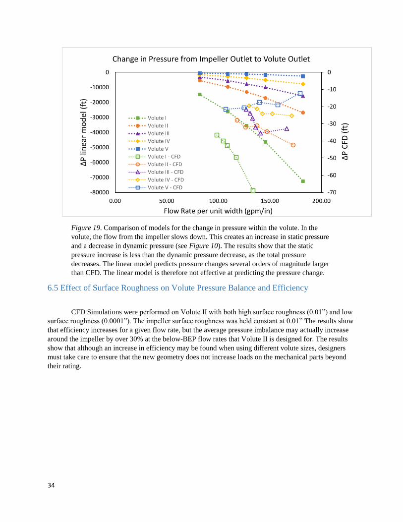
34
Figure 19. Comparison of models for the change in pressure within the volute. In the
volute, the flow from the impeller slows down. This creates an increase in static pressure
and a decrease in dynamic pressure (see Figure 10). The results show that the static
pressure increase is less than the dynamic pressure decrease, as the total pressure
decreases. The linear model predicts pressure changes several orders of magnitude larger
than CFD. The linear model is therefore not effective at predicting the pressure change.
6.5 Effect of Surface Roughness on Volute Pressure Balance and Efficiency
CFD Simulations were performed on Volute II with both high surface roughness (0.01”) and low
surface roughness (0.0001”). The impeller surface roughness was held constant at 0.01” The results show
that efficiency increases for a given flow rate, but the average pressure imbalance may actually increase
around the impeller by over 30% at the below-BEP flow rates that Volute II is designed for. The results
show that although an increase in efficiency may be found when using different volute sizes, designers
must take care to ensure that the new geometry does not increase loads on the mechanical parts beyond
their rating.
-70
-60
-50
-40
-30
-20
-10
0
-80000
-70000
-60000
-50000
-40000
-30000
-20000
-10000
0
0.00 50.00 100.00 150.00 200.00
ΔP
CFD
(ft
)
ΔP
lin
ear
mo
del
(ft
)
Flow Rate per unit width (gpm/in)
Change in Pressure from Impeller Outlet to Volute Outlet
Volute I
Volute II
Volute III
Volute IV
Volute V
Volute I - CFD
Volute II - CFD
Volute III - CFD
Volute IV - CFD
Volute V - CFD

35
Figure 20. Comparison of flow characteristics for a centrifugal pump with different
surface roughness values in the volute. The high roughness of 0.01” inches corresponds
to cast iron, while the low roughness of 0.0001” corresponds to smooth plastic.
Efficiency improves at all points along the head-flow curve, but the average pressure
imbalance across the impeller increases at lower flow rates. The efficiency curves are
normalized with respect to the highest efficiency achieved.
6.6. Life-cycle Cost Analysis of Efficiency and Pressure The power drawn by a pump is directly linked to its efficiency.
𝑃𝑜𝑢𝑡 = 𝜂𝑡𝑜𝑡𝑎𝑙 ∗ 𝑃𝑖𝑛 (6.6.1)
𝜂𝑡𝑜𝑡𝑎𝑙 is the product of all of the efficiencies in the pump, including the volumetric/leakage
efficiency, mechanical efficiency, and hydraulic efficiency. The hydraulic efficiency may also be taken as
the product of the efficiencies of individual sections of the pump, including the inlet piping, impeller,
volute, and outlet. To determine the effect of volute shape on a pump’s operation cost, the volute’s
hydraulic efficiency is taken as a variable, holding the other efficiencies constant. In reality the
efficiencies are linked, but looking just at the volute gives an initial estimate of performance changes.
The estimated hydraulic efficiencies of the volutes are given in Figure 21. The efficiency
calculations illustrate the limitations of a 2D simulation model. The efficiencies curves exhibit multiple
peaks rather that a single best-efficiency point, as is expected in a real pump. The real Xylem pump
0.00
2.00
4.00
6.00
8.00
10.00
70 90 110 130 150 170 190
Avera
ge P
ressure
D
iffe
rence A
cro
ss
Impelle
r (f
t)
High Roughness Low Roughness
0.75
0.8
0.85
0.9
0.95
1
70 90 110 130 150 170 190
No
rma
lize
d H
yd
rau
lic
Effic
iency in IM
PE
LLE
R
+ V
OLU
TE
(-)
Flow Per Unit Width (gpm/inch)
Original BEP Flow
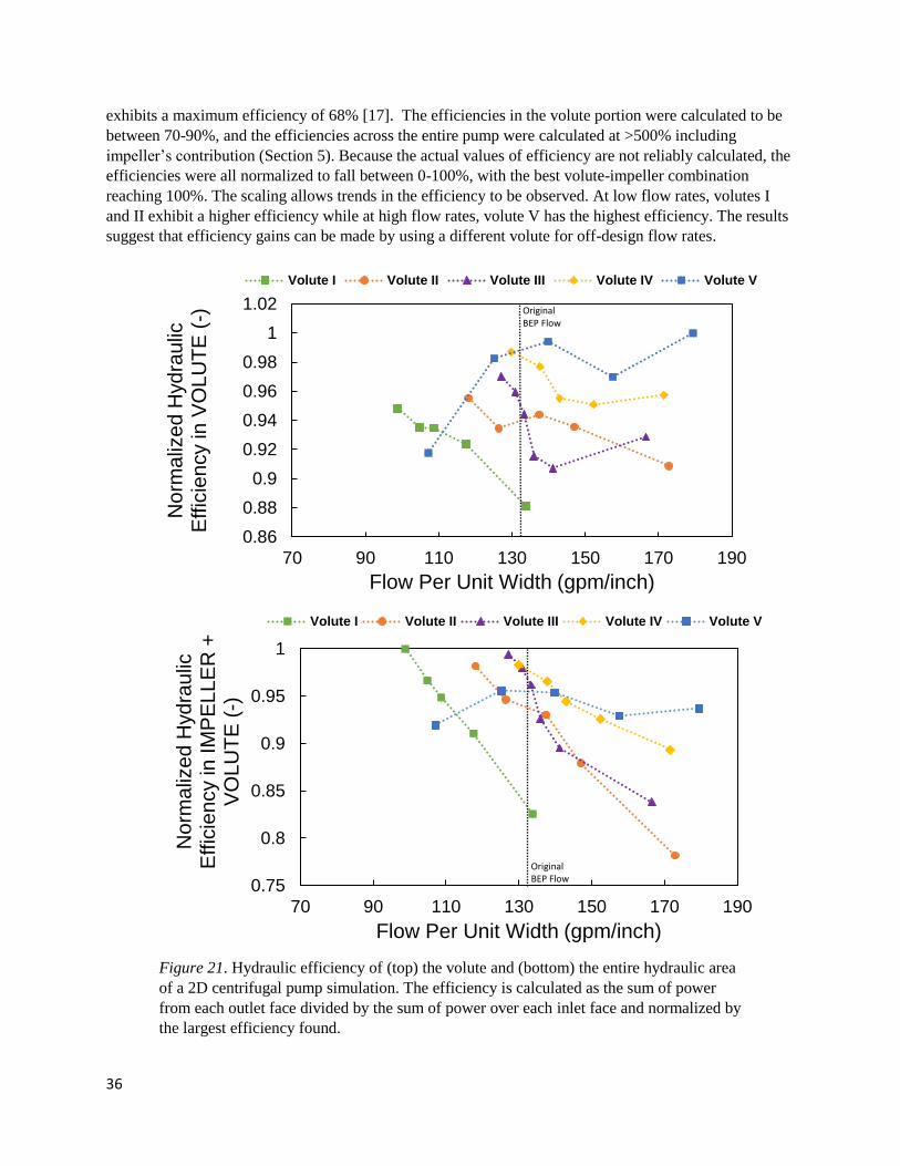
36
exhibits a maximum efficiency of 68% [17]. The efficiencies in the volute portion were calculated to be
between 70-90%, and the efficiencies across the entire pump were calculated at >500% including
impeller’s contribution (Section 5). Because the actual values of efficiency are not reliably calculated, the
efficiencies were all normalized to fall between 0-100%, with the best volute-impeller combination
reaching 100%. The scaling allows trends in the efficiency to be observed. At low flow rates, volutes I
and II exhibit a higher efficiency while at high flow rates, volute V has the highest efficiency. The results
suggest that efficiency gains can be made by using a different volute for off-design flow rates.
Figure 21. Hydraulic efficiency of (top) the volute and (bottom) the entire hydraulic area
of a 2D centrifugal pump simulation. The efficiency is calculated as the sum of power
from each outlet face divided by the sum of power over each inlet face and normalized by
the largest efficiency found.
0.86
0.88
0.9
0.92
0.94
0.96
0.98
1
1.02
70 90 110 130 150 170 190
No
rma
lize
d H
yd
rau
lic
Effic
ien
cy in
VO
LU
TE
(-)
Flow Per Unit Width (gpm/inch)
Volute I Volute II Volute III Volute IV Volute V
Original BEP Flow
0.75
0.8
0.85
0.9
0.95
1
70 90 110 130 150 170 190
No
rma
lize
d H
yd
rau
lic
Effic
ien
cy in
IM
PE
LL
ER
+
VO
LU
TE
(-)
Flow Per Unit Width (gpm/inch)
Volute I Volute II Volute III Volute IV Volute V
Original BEP Flow

37
The lifetime energy cost of a pump is the product of its power input, operation time, and the cost
of energy.
𝐶 = 𝑃𝑖𝑛 ∗ 𝑡 ∗ 𝐸𝑛𝑒𝑟𝑔𝑦 𝐶𝑜𝑠𝑡
Taking Boston as an example, the average commercial electricity cost in May 2019 is
$0.1384/kWh. Experimental results for the pump show the motor demanding 2.6 HP [1939 W] at BEP. If
a pump runs for 24 hours per day, 7 days per week, for 10 years straight, this translates to a lifetime
energy consumption of 163,300 kWh and a total energy cost of $22,600.
Regarding surface roughness, Table 11 suggests that the smoother volute increased in efficiency
by 3.2%. The total power consumption and total cost may be reduced by a factor of 𝜂𝑛𝑒𝑤
𝜂𝑜𝑙𝑑. This would
result in a new total electricity cost of $21,800, an $800 saving over the pump’s lifetime.
If the pump were to be operated at 120% of BEP, Figure 21 indicates that the efficiency could be
improved by as much as 8% if a larger volute (Volute V) were used in place of the original volute (Volute
III). Over 10 years, this would result in a total electricity cost of $20,700, a $19,000 savings.
However, efficiency gains cannot be assumed if a pump’s geometry is being altered. In order to
understand the pump’s overall efficiency, the efficiency of the moving components (mechanical
efficiency) as well as the losses due to leakage (volumetric efficiency) in a more complicated pump
design must be understood [12]. The mechanical and volumetric efficiencies may change when the volute
changes, so understanding the relationship between the three is essential for understanding. This
understanding is currently best achieved by direct measurement.

38
7. Conclusions Three analytical models are presented for predicting the performance of a pump with a
variable-geometry volute casing including: a simplified, linear diffuser model developed by the
author, the momentum-conservation method presented by Iversen et al, and the
momentum/energy-conservation model presented by Iversen et al. These models were used to
analyze a Goulds Water Technology single-stage, radial impeller centrifugal pump. The pump’s
efficiency and impeller pressure imbalance were calculated.
The primary results of the analysis are found in Figure 17, where it is shown that using
a volute that is re-sized for an off-BEP flow rate results in a lower pressure imbalance than
operating the base volute at off-BEP conditions. This result suggests that the cost of pump
maintenance and repair due to mechanical loads will decrease by using a different volute if the
pump is continuously operated at off-design conditions.
The results for efficiency changes with different volutes, Figure 21, suggest that
efficiency is higher in the smaller volute at lower flow rates, and in the larger volute at higher
flow rates, but are inconclusive. The pump’s efficiency is affected by both hydraulic behavior and
mechanical behavior. The mechanical loads on the pump and the resulting mechanical efficiency
are difficult to determine in a 2D simulation, but are beneficial to understand general trends. The
author recommends using 3D CFD to determine the true efficiency, as the flow rate distribution at
the inlet and outlet will be more representative of the patterns in a real pump.
The results verify that a 2D simulation can match the pressure-to-flow relationship of a
real pump if the flow rates are normalized to flow-per-unit-width (Figure 12). Scaling the volute
outlet to maintain the area ratio in 2D was less effective than using the exact cross-section. With
each simulation taking less than two minutes to run, the author recommends the 2D approach as a
way to quickly predict flow characteristics of different volute designs.
It was verified that using a smoother volute wall will increase the efficiency of a
centrifugal pump by reducing frictional losses. However, the results suggest that changing the
volute surface roughness may increase the radial load on the impeller. This could decrease the
pump’s lifetime, even if efficiency gains are seen during normal operation.
Additional conclusions were reached from the assessment of the analytical models in Section 3:
1. The analytical model presented in Iversen [15] (Section 3.3) is problematic because it
doesn’t conserve energy for the flow between the last impeller segment and the first. The
Lorett model (Section 3.4), while more complicated due to the iterative solving process,
provides better results by incorporating energy conservation.
2. The linear channel vastly over-estimates the pressure change in the volute. The
unwrapped volute method is useful for understanding general trends in pressure, but
cannot be relied on to achieve actual pressure measurements
Operating a centrifugal pump at off-design flow rates has traditionally meant a sacrifice
in efficiency and performance. Changing the shape of the volute adds flexibility to the pump by
allowing it to achieve steady pressures across flow rates and improving efficiency at off-design
flow rates.

39
8. References
[1] Gülich, J. F., 2008, Centrifugal Pumps, Springer, Berlin ; New York.
[2] “IBISWorld US - Industry, Company and Business Research Reports and Information” [Online].
Available: https://clients1.ibisworld.ca/reports/us/industry/productsandmarkets.aspx?entid=719.
[Accessed: 21-Mar-2019].
[3] Pedersen, T., Aarsnes, U. J. F., and Godhavn, J.-M., 2018, “Flow and Pressure Control of
Underbalanced Drilling Operations Using NMPC,” J. Process Control, 68, pp. 73–85.
[4] Europump & the Hydraulic Institute, 2004, Variable Speed Pumping: A Guide to Successful
Applications, Elsevier Science, Kidlington, Oxford, UK ; New York.
[5] Arun Shankar, V. K., Umashankar, S., Paramasivam, S., and Hanigovszki, N., 2016, “A
Comprehensive Review on Energy Efficiency Enhancement Initiatives in Centrifugal Pumping
System,” Appl. Energy, 181, pp. 495–513.
[6] Bloch, H. P., and Budris, A. R., 2004, Pump User’s Handbook: Life Extension, CRC Press.
[7] Johnson, H., 2019, “Design of Adaptive Hydraulic Geometries for Improved Centrifugal Pump
Efficiency,” MIT.
[8] Jin, H. B., Kim, M. J., and Chung, W. J., 2012, “A Study on the Effect of Variation of the Cross-
Sectional Area of Spiral Volute Casing for Centrifugal Pump,” 6(8), p. 10.
[9] Baun, D. O., and Flack, R. D., 2003, “Effects of Volute Design and Number of Impeller Blades on
Lateral Impeller Forces and Hydraulic Performance,” Int. J. Rotating Mach. [Online]. Available:
https://www.hindawi.com/journals/ijrm/2003/423094/abs/. [Accessed: 18-Jan-2019].
[10] Worster, W., and Hydraulic Plant and Machinery Group, 1963, “The Flow in Volutes and Its Effect
on Centrifugal Pump Performance,” Proc. Inst. Mech. Eng., 177(1), pp. 843–875.
[11] Busemann, A., 1928, “The Delivery Head of Radial Centrifugal Pumps with Logarithmic Spiral
Blades,” Math Mech, 8(5), p. 372.
[12] Karassik, I. J., Messina, J. P., Cooper, P., and Heald, C. C., 2007, Pump Handbook, McGraw-Hill
Education, New York.
[13] Sayma, N., Computational Fluid Dynamics. 2019. Ventus Publishing ApS
[14] 2003, “Engineering ToolBox, (2003). Density, Specific Weight and Thermal Expansion Coefficient.”
[15] Iversen, H. W., Rolling, R. E., and Carlson, J. J., 1960, “Volute Pressure Distribution, Radial Force
on the Impeller, and Volute Mixing Losses of a Radial Flow Centrifugal Pump,” J. Eng. Power,
82(2), pp. 136–143.
[16] Lorett, J. A., and Gopalakrishnan, S., 1986, “Interaction Between Impeller and Volute of Pumps at
Off-Design Conditions,” J. Fluids Eng., 108(1), p. 12.
[17] Goulds Water Technology, 2017, “B36/3742 R4.”
[18] Elger, D. F., LeBret, B. A., Crowe, C. T., and Roberson, J. A., 2016, Engineering Fluid Mechanics,
John Wiley & Sons, Singapore.
[19] “ANSYS FLUENT 12.0 Tutorial Guide - Problem Description” [Online]. Available:
http://www.afs.enea.it/project/neptunius/docs/fluent/html/tg/node162.htm. [Accessed: 20-Apr-2019].
[20] “Fluent Getting Started Guide,” p. 64.

40
9. Appendix
Additional Volute Parameters Table 6.2
For 60 gpm flow:
Volute I II III IV V
Flow rate (𝑖𝑛3
𝑠𝑒𝑐) 231.00
Flow per average unit width
(𝑖𝑛2
𝑠𝑒𝑐)
420.77
Expected Outlet Head at this
Flow Rate (𝑓𝑡)
107.0 107.65 108.65 107.99 108.0
Impeller inlet velocity (𝑖𝑛
𝑠𝑒𝑐) 147.94
Radial impeller outlet
velocity (𝑖𝑛
𝑠𝑒𝑐)
84.72
Tangential impeller outlet
velocity (𝑖𝑛
𝑠𝑒𝑐)
790.15
α for Q1 (𝑟𝑎𝑑𝑖𝑎𝑛𝑠) 0.11
Velocity at throat (𝑖𝑛
𝑠𝑒𝑐) 682.80 422.93 334.77 251.87 165.77
Reynolds number at throat (-
)
3.3E+07 2.0E+07 1.6E+07 1.2E+07 8.0E+06
Velocity at outlet (𝑖𝑛
𝑠𝑒𝑐) 245.99 245.99 245.99 245.99 245.99
Table 6.3
For 70 gpm flow:
Volute I II III IV V
Flow rate (𝑖𝑛3
𝑠𝑒𝑐) 269.50
Flow per average unit width
(𝑖𝑛2
𝑠𝑒𝑐)
490.89
Expected Outlet Head at this
Flow Rate (𝑓𝑡)
98.0 99.26 101.48 102.17 103.0
Impeller inlet velocity (𝑖𝑛
𝑠𝑒𝑐) 172.60
Radial impeller outlet
velocity (𝑖𝑛
𝑠𝑒𝑐)
98.84
Tangential impeller outlet
velocity (𝑖𝑛
𝑠𝑒𝑐)
757.52
α for Q1 (𝑟𝑎𝑑𝑖𝑎𝑛𝑠) 0.13
Velocity at throat (𝑖𝑛
𝑠𝑒𝑐) 796.61 493.42 390.56 293.85 193.40
Reynolds number at throat (-
)
3.9E+07 2.4E+07 1.9E+07 1.4E+07 9.4E+06
Velocity at outlet (𝑖𝑛
𝑠𝑒𝑐) 286.99 286.99 286.99 286.99 286.99
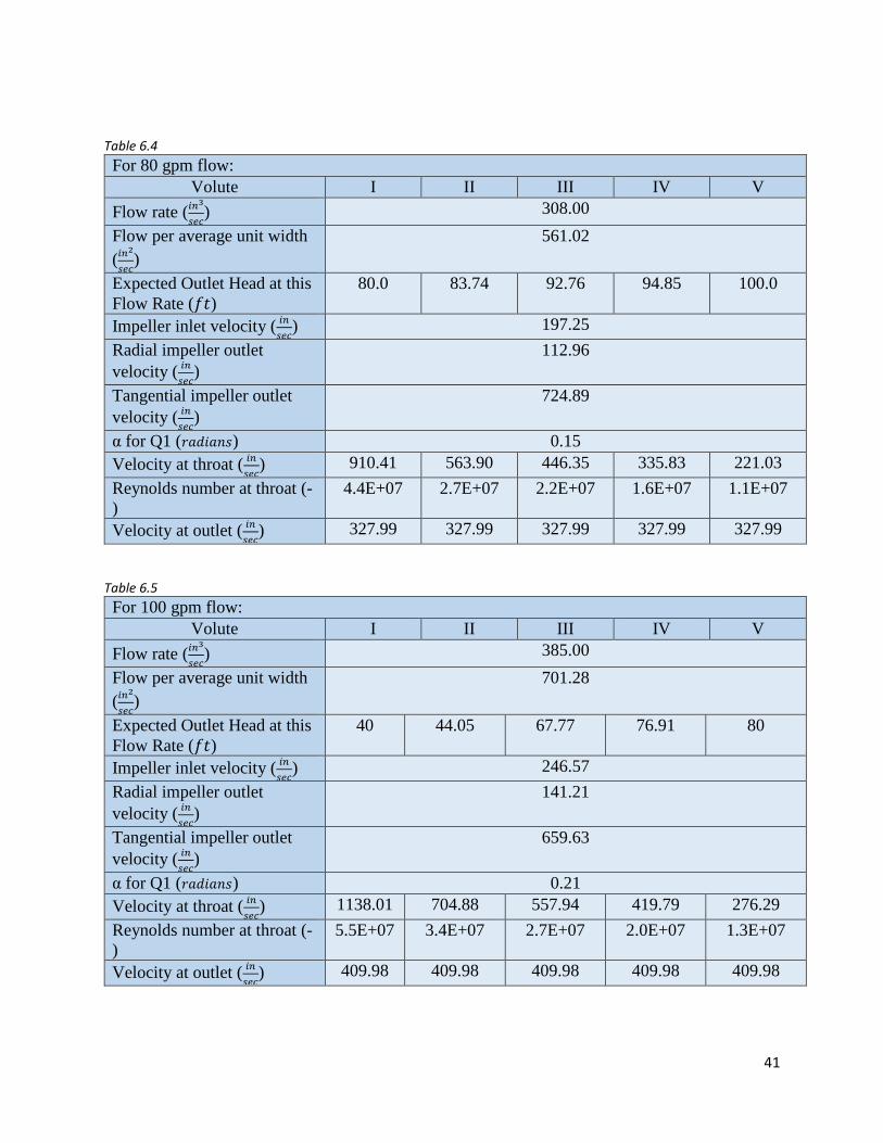
41
Table 6.4
For 80 gpm flow:
Volute I II III IV V
Flow rate (𝑖𝑛3
𝑠𝑒𝑐) 308.00
Flow per average unit width
(𝑖𝑛2
𝑠𝑒𝑐)
561.02
Expected Outlet Head at this
Flow Rate (𝑓𝑡)
80.0 83.74 92.76 94.85 100.0
Impeller inlet velocity (𝑖𝑛
𝑠𝑒𝑐) 197.25
Radial impeller outlet
velocity (𝑖𝑛
𝑠𝑒𝑐)
112.96
Tangential impeller outlet
velocity (𝑖𝑛
𝑠𝑒𝑐)
724.89
α for Q1 (𝑟𝑎𝑑𝑖𝑎𝑛𝑠) 0.15
Velocity at throat (𝑖𝑛
𝑠𝑒𝑐) 910.41 563.90 446.35 335.83 221.03
Reynolds number at throat (-
)
4.4E+07 2.7E+07 2.2E+07 1.6E+07 1.1E+07
Velocity at outlet (𝑖𝑛
𝑠𝑒𝑐) 327.99 327.99 327.99 327.99 327.99
Table 6.5
For 100 gpm flow:
Volute I II III IV V
Flow rate (𝑖𝑛3
𝑠𝑒𝑐) 385.00
Flow per average unit width
(𝑖𝑛2
𝑠𝑒𝑐)
701.28
Expected Outlet Head at this
Flow Rate (𝑓𝑡)
40 44.05 67.77 76.91 80
Impeller inlet velocity (𝑖𝑛
𝑠𝑒𝑐) 246.57
Radial impeller outlet
velocity (𝑖𝑛
𝑠𝑒𝑐)
141.21
Tangential impeller outlet
velocity (𝑖𝑛
𝑠𝑒𝑐)
659.63
α for Q1 (𝑟𝑎𝑑𝑖𝑎𝑛𝑠) 0.21
Velocity at throat (𝑖𝑛
𝑠𝑒𝑐) 1138.01 704.88 557.94 419.79 276.29
Reynolds number at throat (-
)
5.5E+07 3.4E+07 2.7E+07 2.0E+07 1.3E+07
Velocity at outlet (𝑖𝑛
𝑠𝑒𝑐) 409.98 409.98 409.98 409.98 409.98

42
MATLAB code for analyzing CFD data
function
[hydraulic_efficiency,hydraulic_efficiency_volute,weighted_pressure_difference_ft,flow
_per_width,interface_angle_deg,interface_pressures_ft] =
Fluent_volute_analysis(xcoordinate,ycoordinate,xvelocity,yvelocity,totalpressure,stati
cpressure)
% Analyzes raw data exported from Fluent 2D simulation of centrifugal pump
% inputs are xvelocity, yvelocity, static pressure, and total pressure
% Created by Daly Wettermark 5/1/19
% Last modified by Daly Wettermark 5/13/19
%Analysis of raw data for FLUENT simulation
% CONVERSIONS
in_per_m = 39.3701; %conversion from meters to inches
ft_h2o_per_pascal = 0.00033455; % conversion from pascals to feet of water
vel_scale = 200; % scaling factor for plotting large velocity vectors
gpm_per_m3persec = 15850.37; % conversion from m3/sec to gpm
Patm = 101325; %Pa, atmospheric pressure
absolutepressure = totalpressure + 101325; %add atmospheric pressure
% USER-DEFINED PARAMETERS FROM SIMULATION
impeller_diameter = 5.390/in_per_m; % meters
inlet_diameter = 1.4/in_per_m; % meters
mesh_size = 0.04/in_per_m; % minimum mesh size, meters
x = xcoordinate;
y = ycoordinate;
% FIND NODES AT VOLUTE INLET AND INTERFACE
radius = sqrt(x.^2 + y.^2); % finds distance from origin to each node
% calculate normal angle from volute cutwater using x and y
% coordinates. The impeller center is at (0,0).
normal_angle = zeros(length(x),1);
for index = 1:length(x)
if (x(index) > 0) && (y(index) > 0) % first quadrant
normal_angle(index) = atan(y(index)/x(index));
elseif x(index) > 0 && y(index) < 0 % fourth quadrant
normal_angle(index) = 2*pi - abs(atan(y(index)/x(index)));
elseif x(index) < 0 && y(index) < 0 % third quadrant
normal_angle(index) = atan(y(index)./x(index))+pi;
elseif x(index) < 0 && y(index) > 0 % second quadrant
normal_angle(index) = pi - abs(atan(y(index)./x(index)));
end

43
end
% find nodes beyond the impeller, i.e. the volute hydraulic area.
% They are located at a distance of "impeller_diameter" from the
% origin, +/- a small variation due to mesh size. Ignores the area
% beyond the volute throat in the outlet section.
volute = find((radius >= (impeller_diameter/2 + mesh_size) & normal_angle > 0.9) |
(radius >= (impeller_diameter/2 + mesh_size) & radius < 0.0745 & normal_angle <=
0.9));
% Find indices of the nodes along the impeller inlet
inlet_indices = find(radius < inlet_diameter/2 + mesh_size/5);
% Find indices of the nodes along the impeller periphery/volute interface
interface_indices = find(radius >= impeller_diameter/2 - 0.01/in_per_m/20 & radius
< impeller_diameter/2 + 0.01/in_per_m/20);
% Uncomment next line to check if values are correct
% figure(); plot(x(interface_indices),y(interface_indices),'.'); hold on;
plot(x(inlet_indices),y(inlet_indices),'.')
% To get indices of the volute outlet, you must first plot all of the nodes
% and find the x-location of the outlet. Uncomment next line to do that.
% figure(); plot(x,y,'.')
y_outlet = 0.0660; %manually input y-location of outlet
x_min_outlet = 0.07499; % manually input x-location of lowest node of outlet
% FIND NODES AT VOLUTE OUTLET
outlet_indices_y = find(y > y_outlet - mesh_size/10 & y < y_outlet +
mesh_size/10);
outlet_indices_x = find(x >= x_min_outlet - 0.01/2);
similar_values = ismember(outlet_indices_y,outlet_indices_x);
outlet_indices = (outlet_indices_y(similar_values));
%plot(x(outlet_indices),y(outlet_indices),'.');
% CALCULATE NORMAL VELOCITY AT VOLUTE INTERFACE AND OUTLET
% for inlet and interface, it depends on the location around the impeller circle
%initialize normal_angle vector
normal_angle_inlet = zeros(length(inlet_indices),1);
for index = 1:length(inlet_indices)
face = inlet_indices(index);
if (x(face) > 0) && (y(face) > 0) % first quadrant
normal_angle_inlet(index) = atan(y(face)/x(face));
elseif x(face) > 0 && y(face) < 0 % fourth quadrant
normal_angle_inlet(index) = 2*pi - abs(atan(y(face)/x(face)));
elseif x(face) < 0 && y(face) < 0 % third quadrant
normal_angle_inlet(index) = atan(y(face)./x(face))+pi;
elseif x(face) < 0 && y(face) > 0 % second quadrant
normal_angle_inlet(index) = pi - abs(atan(y(face)./x(face)));

44
end
end
normal_angle_interface = zeros(length(interface_indices),1);
for index = 1:length(interface_indices)
face = interface_indices(index);
if (x(face) > 0) && (y(face) > 0)
normal_angle_interface(index) = atan(y(face)/x(face));
elseif x(face) > 0 && y(face) < 0
normal_angle_interface(index) = 2*pi - abs(atan(y(face)/x(face)));
elseif x(face) < 0 && y(face) < 0
normal_angle_interface(index) = atan(y(face)./x(face))+pi;
elseif x(face) < 0 && y(face) > 0
normal_angle_interface(index) = pi - abs(atan(y(face)./x(face)));
end
end
normal_angle_outlet = zeros(length(outlet_indices),1);
% SORT INDEX VECTORS FOR INLET & INTERFACE TO BE IN ORDER OF NORMAL ANGLE
[normal_angle_inlet, inlet_sorted_indices] = sort(normal_angle_inlet);
inlet_indices = inlet_indices(inlet_sorted_indices);
[normal_angle_interface, interface_sorted_indices] = sort(normal_angle_interface);
interface_indices = interface_indices(interface_sorted_indices);
% SORT INLET VECTORS AGAIN SO THAT THE FIRST ENTRY IS THE START OF AN INLET
SECTION
inlet_angle_differences = abs(normal_angle_inlet(1:end-1) -
normal_angle_inlet(2:end));
start_locations = find(inlet_angle_differences > pi/12);
start_locations = start_locations + 1;
% for outlet, the angle is everywhere zero
normal_angle_outlet = 0;
quiver_plots = 0;
%% CALCULATIONS
% Calculate node’s “surface area” at volute interface and outlet
% Calculate pressure difference on opposite sides of impeller
% Calculate volumetric flow rate through each node’s “suface area” in square inches
per second
% for inlet
% separate outlet locations into six segments since the outlet is not a full
circle
sections = 6; % number of sections

45
flow_inlet = zeros(length(inlet_indices),1); % initialize
length_inlet_edges = zeros(length(inlet_indices),1); % initialize
radial_velocity_inlet = zeros(length(inlet_indices),1);
for section = 1:sections
if section == sections % if this is the last section
% create subset of index and angle values for the specific inlet section
index_subset =
[inlet_indices(start_locations(section):end);inlet_indices(1:start_locations(1)-1)];
angle_subset =
[normal_angle_inlet(start_locations(section):end);normal_angle_inlet(1:start_locations
(1)-1)];
else
index_subset =
inlet_indices(start_locations(section):start_locations(section+1)-1);
angle_subset =
normal_angle_inlet(start_locations(section):start_locations(section+1)-1);
end
for face = 1:length(index_subset)
if start_locations(section)+face-1 <= length(inlet_indices)
if face == 1
length_inlet_edges(start_locations(section)) =
abs(inlet_diameter/2*(angle_subset(2) - angle_subset(1))/2);
elseif face == length(index_subset)
length_inlet_edges(start_locations(section)+face-1) =
abs(inlet_diameter/2*((angle_subset(end) - angle_subset(end-1))/2));
else
if abs(angle_subset(face-1)-angle_subset(face+1)) > pi
length_inlet_edges(start_locations(section)+face-1) =
abs(inlet_diameter/2*(angle_subset(face-1)-angle_subset(face+1)-2*pi)/2);
else
length_inlet_edges(start_locations(section)+face-1) =
abs(inlet_diameter/2*(angle_subset(face-1)-angle_subset(face+1))/2);
end
end
radial_velocity_inlet(start_locations(section)+face-1) =
dot([xvelocity(index_subset(face)),yvelocity(index_subset(face))],[cos(angle_subset(fa
ce)),sin(angle_subset(face))]); % radial velocity is the portion of velocity normal to
the surface – this is the velocity that contributes to flow rate
flow_inlet(start_locations(section)+face-1) =
length_inlet_edges(start_locations(section)+face-
1)*radial_velocity_inlet(start_locations(section)+face-1);
hold on
if quiver_plots == 1 % plot velocity vector at edge
quiver(x(index_subset(face)),y(index_subset(face)),radial_velocity_inlet(start_locatio
ns(section)+face-
1)/vel_scale*cos(angle_subset(face)),radial_velocity_inlet(start_locations(section)+fa
ce-1)/vel_scale*sin(angle_subset(face)),'Color','b')
end
else

46
if face == length(index_subset)
length_inlet_edges(start_locations(section)+face-1-
length(inlet_indices)) = abs(inlet_diameter/2*((angle_subset(end) - angle_subset(end-
1))));
else % check if we are at the end of the angle vector, looping back
from 2*pi to zero
if angle_subset(face-1)-angle_subset(face+1) > pi
length_inlet_edges(start_locations(section)+face-1-
length(inlet_indices)) = abs(inlet_diameter/2*(angle_subset(face-1)-
angle_subset(face+1)-2*pi)/2); % if so, 2*pi is subtracted from angle difference
else
length_inlet_edges(start_locations(section)+face-1-
length(inlet_indices)) = abs(inlet_diameter/2*(angle_subset(face-1)-
angle_subset(face+1))/2);
end
end
radial_velocity_inlet(start_locations(section)+face-1-
length(inlet_indices)) =
dot([xvelocity(index_subset(face)),yvelocity(index_subset(face))],[cos(angle_subset(fa
ce)),sin(angle_subset(face))]);
flow_inlet(start_locations(section)+face-1-length(inlet_indices)) =
length_inlet_edges(start_locations(section)+face-1-
length(inlet_indices))*radial_velocity_inlet(start_locations(section)+face-1-
length(inlet_indices)); % flow = area (or length in this case) * normal velocity
hold on
if quiver_plots == 1
quiver(x(index_subset(face)),y(index_subset(face)),radial_velocity_inlet(start_locatio
ns(section)+face-1-
length(inlet_indices))/vel_scale*cos(angle_subset(face)),radial_velocity_inlet(start_l
ocations(section)+face-1-
length(inlet_indices))/vel_scale*sin(angle_subset(face)),'Color','b')
end
end
end
end
% for interface
% similar procedure as inlet, but one continuous section rather than separate
sections
flow_interface = zeros(length(interface_indices),1);
length_interface_edges = zeros(length(interface_indices),1);
weighted_pressure_differences = zeros(floor(length(interface_indices)/2),1); %
initialize
radial_velocity_interface = zeros(length(interface_indices),1); % initialize
% the length of each edge is half the angular distance between the points to the left
or right of it multiplied by the radius. If a uniform mesh size was used, these values
should all be equal or very similar
for face = 1:length(interface_indices)

47
if face == 1
length_interface_edges(1) =
abs(impeller_diameter/2*(normal_angle_interface(length(interface_indices))-2*pi-
normal_angle_interface(2))/2);
elseif face == length(interface_indices)
length_interface_edges(face) =
abs(impeller_diameter/2*(normal_angle_interface(length(interface_indices)-1)-2*pi-
normal_angle_interface(1))/2);
else
length_interface_edges(face) =
abs(impeller_diameter/2*(normal_angle_interface(face-1)-
normal_angle_interface(face+1))/2);
end
radial_velocity_interface(face) =
dot([xvelocity(interface_indices(face)),yvelocity(interface_indices(face))],[cos(norma
l_angle_interface(face)),sin(normal_angle_interface(face))]);
flow_interface(face) =
length_interface_edges(face).*radial_velocity_interface(face);
if quiver_plots == 1
hold on
quiver(x(interface_indices(face)),y(interface_indices(face)),radial_velocity_interface
(face)/vel_scale*cos(normal_angle_interface(face)),radial_velocity_interface(face)/vel
_scale*sin(normal_angle_interface(face)),'Color','g')
end
if face < length(interface_indices)/2
pressure_difference = abs(staticpressure(interface_indices(face))-
staticpressure(interface_indices(face+floor(length(interface_indices)/2))));
weighted_pressure_differences(face) =
pressure_difference*length_interface_edges(face);
end
end
weighted_pressure_differences =
weighted_pressure_differences./sum(length_interface_edges);
weighted_pressure_difference = sum(weighted_pressure_differences);
weighted_pressure_difference_ft = weighted_pressure_difference *
ft_h2o_per_pascal;
% for outlet
flow_outlet = zeros(length(outlet_indices),1); % initialize
length_outlet_edges = zeros(length(outlet_indices),1); % initialize
for face = 1:length(outlet_indices)
% the length of each edge is half the distance between the points to the left
or right of it. If a uniform mesh size was used, these values should all be equal
if face == 1
length_outlet_edges(1) = abs(x(outlet_indices(2))-x(outlet_indices(1)));
elseif face == length(outlet_indices)

48
length_outlet_edges(face) = abs(x(outlet_indices(face))-
x(outlet_indices(face-1)));
else
length_outlet_edges(face) = abs(x(outlet_indices(face+1))-
x(outlet_indices(face-1)))/2;
end
flow_outlet(face) =
length_outlet_edges(face).*yvelocity(outlet_indices(face));
if quiver_plots == 1
quiver(x(outlet_indices(face)),y(outlet_indices(face)),0,yvelocity(outlet_indices(face
))/vel_scale,'Color','r')
end
end
axis equal
% Create pressure contour plots
contour = 0;
if contour == 1
% 2D plot
CircleSize = 70;
figure;h2=scatter3(normal_angle(volute(1:end-
5))*360/(2*pi),radius(volute(1:end-5)),staticpressure(volute(1:end-
5)),CircleSize,totalpressure(volute(1:end-5)),'s','filled');
view(2);
xlabel('Angular Position from Cutwater (degrees)')
ylabel('Radius (m)')
%3D plot
figure()
subplot(1,2,1)
% triangulate and plot
tri = delaunay(normal_angle(volute(1:end-5))*360/(2*pi),radius(volute(1:end-
5)));
trisurf(tri, normal_angle(volute(1:end-5))*360/(2*pi),radius(volute(1:end-
5))*in_per_m,staticpressure(volute(1:end-5))*ft_h2o_per_pascal);
shading interp
xlabel('Angular Position from Cutwater (degrees)','FontSize',16)
xlim([0,350])
ylabel('Radius (inches)','FontSize',16)
zlabel('Static Pressure (ft)','FontSize',18)
subplot(1,2,2)
trisurf(tri, normal_angle(volute(1:end-5))*360/(2*pi),radius(volute(1:end-
5))*in_per_m,totalpressure(volute(1:end-5))*ft_h2o_per_pascal);
shading interp
xlabel('Angular Position from Cutwater (degrees)','FontSize',16)
xlim([0,350])
ylabel('Radius (inches)','FontSize',16)
zlabel('Total Pressure (ft)','FontSize',18)

49
end
% CALCULATE POWER PER UNIT WIDTH AT INLET, VOLUTE INTERFACE, AND OUTLET
% power = flow rate * total pressure
power_inlet = sum(flow_inlet.*absolutepressure(inlet_indices));
power_interface = sum(flow_interface.*absolutepressure(interface_indices));
power_outlet = sum(flow_outlet.*absolutepressure(outlet_indices));
flow_per_width = sum(flow_outlet) * gpm_per_m3persec / in_per_m; % flow in gpm,
divided by width of simulation area (1m)
% Calculate efficiency at the ratio of outlet power to inlet power
hydraulic_efficiency_volute = power_outlet/power_interface;
hydraulic_efficiency = power_outlet/power_inlet;
% Create vectors of pressure along interface and angular position
interface_pressures_ft = totalpressure(interface_indices) * ft_h2o_per_pascal;
interface_angle_deg = normal_angle_interface.*360/(2*pi);
end
Published with MATLAB® R2016b
MATLAB code for calculating model in section 3.2 from impeller outlet to throat
% Purpose: Solving for pressures at inlet and outlet of impeller using momentum
% balance equations
% Created 2-23-2019 Daly Wettermark
% Last Modified 5-16-2019 Daly Wettermark [email protected]
syms rho a3 D phi Q alpha Pthroat P3 v2 v3 x y b2 b3 real
% 3D - with width
v2_y = Q/(pi*D*b2);
v3 = Q/(a3*b3);
v2vec = [v2_y/tan(alpha) ; v2_y];
v3vec = [v3 ; 0];
n2 = [0 ; -1];
n3 = [1 ; 0];
n4 = [-sin(phi) ; cos(phi)];
% Expression for time rate of change of momentum
% 2 x 1 vectors for x and y components
DpDt_2 = -int(rho*v2vec*dot(v2vec,n2), x, 0, a3)*b2;
DpDt_3 = -int(rho*v3vec*dot(v3vec,n3), y, 0, pi*D)*b3;

50
DpDt = DpDt_2 + DpDt_3;
% Expression for Body forces
% 2 x 1 vector for x and y components
SigmaF = (-pi * D * b2 * Pthroat * n2) + (- a3 * b3 * P3 * n3) - (int((Pthroat + (P3 -
Pthroat)*x/(pi*D)),x,0,pi*D)*n4*b3/cos(phi));
% Separate equations into x and y
balance_x = DpDt(1) + SigmaF(1);
balance_y = DpDt(2) + SigmaF(2);
% Solve for pressures
P_throat_x = solve(balance_x,P3);
P_throat_y = solve(balance_y,P3);
P_2 = solve(P_throat_x == P_throat_y, Pthroat);
P_2 = simplify(P_2)
P_2_x = solve(balance_x,Pthroat);
P_2_y = solve(balance_y,Pthroat);
P_3 = solve(P_2_x == P_2_y, P3);
P_3 = simplify(P_3)
Symbolic answers:
P_2 =(Q^2*rho*(2*a3^4*b3*cos(phi)*sin(alpha) + D^4*b2*pi^4*cos(phi)*sin(alpha) -
pi*D*a3^3*b3*cos(alpha)*cos(phi) -
pi*D*a3^3*b3*sin(alpha)*sin(phi)))/(D^3*a3^2*b2*b3*pi^3*sin(alpha)*(a3*b3*cos(phi) -
2*a3*b2*cos(phi) + pi*D*b2*sin(phi)))
P_3 =(Q^2*rho*(a3^3*b3^2*cos(alpha)*cos(phi) + a3^3*b3^2*sin(alpha)*sin(phi) +
2*D^3*b2^2*pi^3*cos(phi)*sin(alpha) - 2*a3^3*b2*b3*cos(alpha)*cos(phi) -
D^3*b2*b3*pi^3*cos(phi)*sin(alpha)))/(D^2*a3^2*b2*b3^2*pi^2*sin(alpha)*(a3*b3*cos(phi)
- 2*a3*b2*cos(phi) + pi*D*b2*sin(phi)))