Modeling Electromechanical Overcurrent Relays Using ...downloads.hindawi.com/journals/jam/2012/104952.pdf · some older relays have been replaced by new digital ones, there are still

Hindawi Publishing CorporationJournal of Applied MathematicsVolume 2012, Article ID 104952, 18 pagesdoi:10.1155/2012/104952

Research ArticleModeling Electromechanical Overcurrent RelaysUsing Singular Value Decomposition

Feng-Jih Wu,1 Chih-Ju Chou,1 Ying Lu,2 and Jarm-Long Chung3

1 Department of Electrical Engineering, National Taipei University of Technology, Taipei 10608, Taiwan2 Department of Computer and Communication Engineering, St. John’s University, Tamsui District, NewTaipei City 25135, Taiwan

3 Department of Power Supply, Taiwan Power Company, Zhongzheng District, Taipei City 10016, Taiwan

Correspondence should be addressed to Feng-Jih Wu, [email protected]

Received 17 August 2012; Accepted 5 November 2012

Academic Editor: Ricardo Perera

Copyright q 2012 Feng-Jih Wu et al. This is an open access article distributed under the CreativeCommons Attribution License, which permits unrestricted use, distribution, and reproduction inany medium, provided the original work is properly cited.

This paper presents a practical and effective novel approach to curve fit electromechanical (EM)overcurrent (OC) relay characteristics. Based on singular value decomposition (SVD), the curvesare fitted with equation in state space under modal coordinates. The relationships between transferfunction and Markov parameters are adopted in this research to represent the characteristiccurves of EM OC relays. This study applies the proposed method to two EM OC relays: the GEIAC51 relay with moderately inverse-time characteristic and the ABB CO-8 relay with inverse-time characteristic. The maximum absolute values of errors of hundreds of sample points takenfrom four time dial settings (TDS) for each relay between the actual characteristic curves and thecorresponding values from the curve-fitting equations are within the range of 10 milliseconds.Finally, this study compares the SVD with the adaptive network and fuzzy inference system(ANFIS) to demonstrate its accuracy and identification robustness.

1. Introduction

Power generation systems generally have few large generators connected directly to theirsubtransmission networks and distribution networks. Thus, the fault currents of busesdo not differ much from those of transmission lines. This makes low-cost, reliable, andeasily coordinated electromechanical (EM) overcurrent (OC) relays suitable for protectioncoordination relay in the subtransmission networks and distribution networks. Althoughsome older relays have been replaced by new digital ones, there are still many EM OC relaysin service.

The operation principle of the EM OC relay is to introduce an electric current intothe coil of an electromagnet to produce eddy currents with phase differences. This in turn

2 Journal of Applied Mathematics

generates induction torque on the rotation disc of the relay. The proper contact closing timecan be set by adjusting the distance between the fixed and the movable contacts, achievingprotection coordination between upstream and downstream. However, due to themechanicalnature of the relay, there are inertial and frictional effects. Therefore, unlike a digital relay[1], it is not possible to describe the characteristic curve of an EM OC relay using a singleprecise equation. Manufacturer manuals generally provide families of characteristic curveswith different time dial (TDS) values. These are all piecewise nonlinear continuous smoothdescending curves.

Accurate representations of the inverse-time EM OC relay characteristics play animportant role in the coordination of power network protection schemes. In the early days,researchers were interested in fitting EM OC relay characteristics curves [2] to facilitateprotection coordination in conventional power systems. After the introduction of the digitalOC relays, better curve-fitting of EM OC relay characteristic [3–6] is even more important forproper protection coordination. Most of the literature about curve fitting shows the absolutevalues of errors [7–9], while some show the averages of absolute values of errors [9, 10].Only a few studies show the maximum absolute values of percentage errors [10], which areharder to curve fit, and no studies show themaximum absolute values of errors, which are thehardest to curve fit. For EM OC relays at small values of M (multiples of tap value current),for example, 1.3–3.5, the relay operating time changes nonlinearly and drastically, and onlyone study [10] shows the curve fitting results in this range of M values.

This paper applies the Hankel matrices and the singular value decomposition (SVD)[11–13] to obtain the curve-fitting equation of the characteristic curves of two EM OC relaysunder state space with modal coordinates [14, 15]. To demonstrate the accuracy of the curve-fitting results, the current study not only shows all the maximum absolute values of errors,maximum absolute values of percentage errors, average of absolute values of errors, andaverage of absolute values of percentage errors, but also considers smaller values ofMwherethe relay operating time changes nonlinearly and drastically. For even better accuracy, thispaper reduces the maximum absolute values of errors to less than an alternating current cyclein the range of a few milliseconds (ms), as opposed to 3 cycles in [3] or 2 cycles in [8].

The paper proposed a new application algorithm to fit the characteristic curves of theEMOC relays, using one unified equation to represent their characteristics. Finally, this studyuses the SVD method to fit the characteristic curves of EM OC relays. Comparing the resultswith those obtained by [9] demonstrates the accuracy and identification robustness of theSVD method.

The content of this paper is as follows: Section 2 introduces the representations for thecharacteristic curves of EM OC relays, the mathematical derivation of the curve fitting of thecharacteristic curves of the EM OC relays using SVD method is outlined in Section 3, twocases are studied in Section 4 to verify the approach, the performance of the SVD and thewell-behaved ANFIS algorithm are compared in Section 5, and the conclusion is in Section 6.

2. Models of the Electromechanical (EM)Overcurrent (OC) Relay Characteristic

The characteristic of an EM OC relay is determined by its magnetic circuit design, andthe manufacturers provide the characteristics in the relay manuals with curves in a two-dimensional plot with M the abscissa and operating time the ordinate. Some typical modelsfor the characteristic of an EM OC relay are as follows.

Journal of Applied Mathematics 3

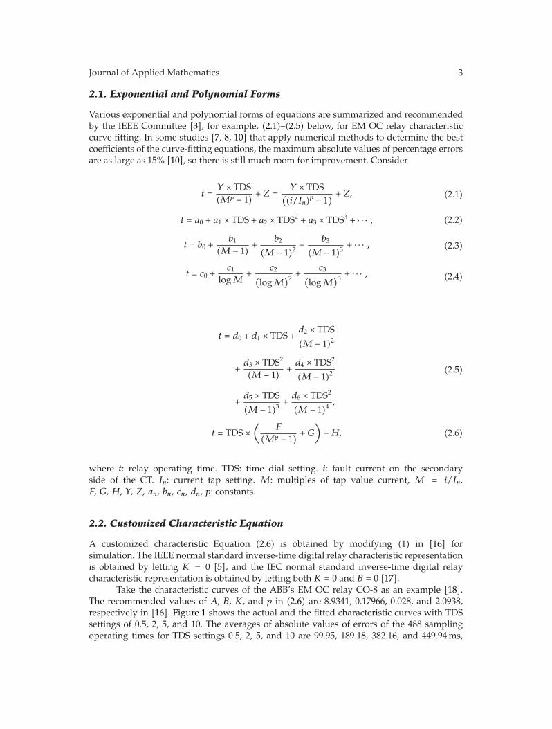
2.1. Exponential and Polynomial Forms

Various exponential and polynomial forms of equations are summarized and recommendedby the IEEE Committee [3], for example, (2.1)–(2.5) below, for EM OC relay characteristiccurve fitting. In some studies [7, 8, 10] that apply numerical methods to determine the bestcoefficients of the curve-fitting equations, the maximum absolute values of percentage errorsare as large as 15% [10], so there is still much room for improvement. Consider

t =Y × TDS(Mp − 1)

+ Z =Y × TDS

((i/In)

p − 1) + Z, (2.1)

t = a0 + a1 × TDS + a2 × TDS2 + a3 × TDS3 + · · · , (2.2)

t = b0 +b1

(M − 1)+

b2

(M − 1)2+

b3

(M − 1)3+ · · · , (2.3)

t = c0 +c1

logM+

c2(logM

)2 +c3

(logM

)3 + · · · , (2.4)

t = d0 + d1 × TDS +d2 × TDS

(M − 1)2

+d3 × TDS2

(M − 1)+d4 × TDS2

(M − 1)2

+d5 × TDS

(M − 1)3+d6 × TDS2

(M − 1)4,

(2.5)

t = TDS ×(

F

(Mp − 1)+G

)+H, (2.6)

where t: relay operating time. TDS: time dial setting. i: fault current on the secondaryside of the CT. In: current tap setting. M: multiples of tap value current, M = i/In.F, G, H, Y, Z, an, bn, cn, dn, p: constants.

2.2. Customized Characteristic Equation

A customized characteristic Equation (2.6) is obtained by modifying (1) in [16] forsimulation. The IEEE normal standard inverse-time digital relay characteristic representationis obtained by letting K = 0 [5], and the IEC normal standard inverse-time digital relaycharacteristic representation is obtained by letting both K = 0 and B = 0 [17].

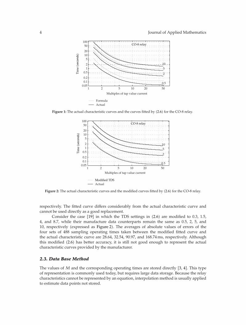
Take the characteristic curves of the ABB’s EM OC relay CO-8 as an example [18].The recommended values of A, B, K, and p in (2.6) are 8.9341, 0.17966, 0.028, and 2.0938,respectively in [16]. Figure 1 shows the actual and the fitted characteristic curves with TDSsettings of 0.5, 2, 5, and 10. The averages of absolute values of errors of the 488 samplingoperating times for TDS settings 0.5, 2, 5, and 10 are 99.95, 189.18, 382.16, and 449.94ms,


1 2 5 10 20 500.050.10.2

0.512

51020

50100

Multiples of tap value current

FormulaActual

5

0.5

10

2

CO-8 relay

Tim

e(secon

ds)

Figure 1: The actual characteristic curves and the curves fitted by (2.6) for the CO-8 relay.

1 2 5 10 20 500.050.10.2

0.512

51020

50100

ActualModified TDS

CO-8 relay


Tim

e(secon

ds)

5

0.5

10

2

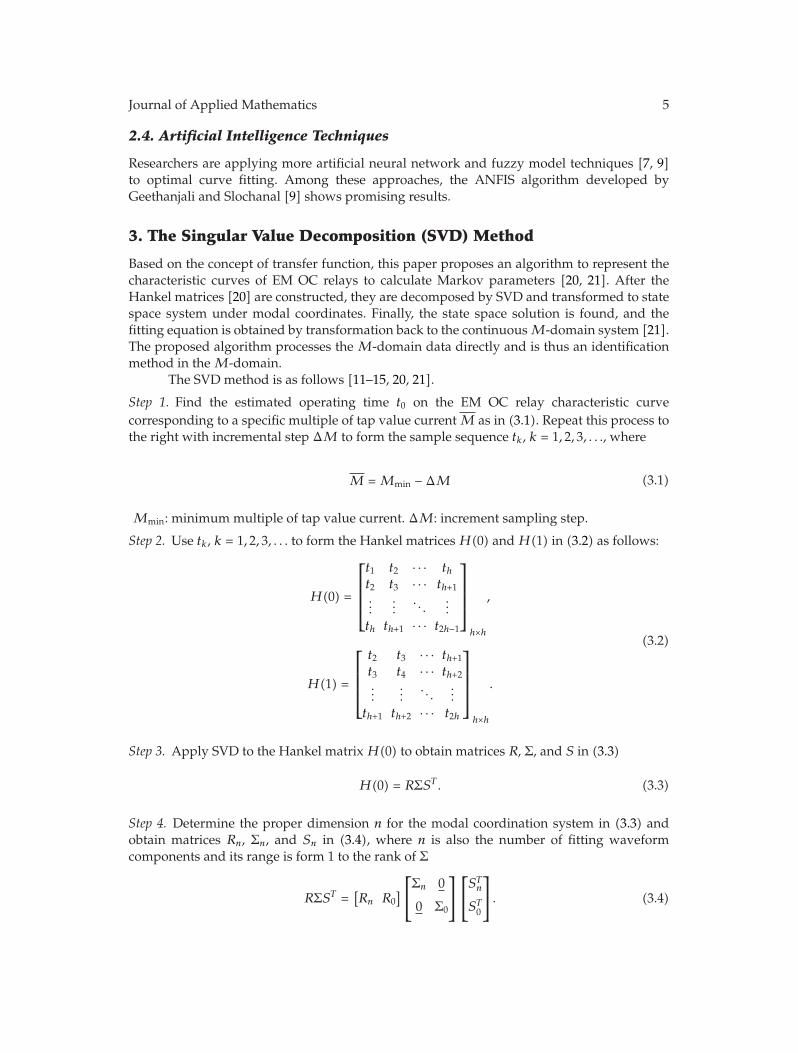
Figure 2: The actual characteristic curves and the modified curves fitted by (2.6) for the CO-8 relay.

respectively. The fitted curve differs considerably from the actual characteristic curve andcannot be used directly as a good replacement.

Consider the case [19] in which the TDS settings in (2.6) are modified to 0.3, 1.5,4, and 8.7, while their manufacture data counterparts remain the same as 0.5, 2, 5, and10, respectively (expressed as Figure 2). The averages of absolute values of errors of thefour sets of 488 sampling operating times taken between the modified fitted curve andthe actual characteristic curve are 28.64, 32.54, 90.97, and 168.74ms, respectively. Althoughthis modified (2.6) has better accuracy, it is still not good enough to represent the actualcharacteristic curves provided by the manufacturer.

2.3. Data Base Method

The values of M and the corresponding operating times are stored directly [3, 4]. This typeof representation is commonly used today, but requires large data storage. Because the relaycharacteristics cannot be represented by an equation, interpolation method is usually appliedto estimate data points not stored.


2.4. Artificial Intelligence Techniques

Researchers are applying more artificial neural network and fuzzy model techniques [7, 9]to optimal curve fitting. Among these approaches, the ANFIS algorithm developed byGeethanjali and Slochanal [9] shows promising results.

3. The Singular Value Decomposition (SVD) Method

Based on the concept of transfer function, this paper proposes an algorithm to represent thecharacteristic curves of EM OC relays to calculate Markov parameters [20, 21]. After theHankel matrices [20] are constructed, they are decomposed by SVD and transformed to statespace system under modal coordinates. Finally, the state space solution is found, and thefitting equation is obtained by transformation back to the continuousM-domain system [21].The proposed algorithm processes the M-domain data directly and is thus an identificationmethod in the M-domain.

The SVD method is as follows [11–15, 20, 21].

Step 1. Find the estimated operating time t0 on the EM OC relay characteristic curvecorresponding to a specific multiple of tap value currentM as in (3.1). Repeat this process tothe right with incremental step ΔM to form the sample sequence tk, k = 1, 2, 3, . . ., where

M = Mmin −ΔM (3.1)

Mmin: minimum multiple of tap value current. ΔM: increment sampling step.

Step 2. Use tk, k = 1, 2, 3, . . . to form the Hankel matrices H(0) andH(1) in (3.2) as follows:

H(0) =

⎡

⎢⎢⎢⎣

t1 t2 · · · tht2 t3 · · · th+1...

.... . .

...th th+1 · · · t2h−1

⎤

⎥⎥⎥⎦

h×h

,

H(1) =

⎡

⎢⎢⎢⎣

t2 t3 · · · th+1t3 t4 · · · th+2...

.... . .

...th+1 th+2 · · · t2h

⎤

⎥⎥⎥⎦

h×h

.

(3.2)

Step 3. Apply SVD to the Hankel matrix H(0) to obtain matrices R, Σ, and S in (3.3)

H(0) = RΣST . (3.3)

Step 4. Determine the proper dimension n for the modal coordination system in (3.3) andobtain matrices Rn, Σn, and Sn in (3.4), where n is also the number of fitting waveformcomponents and its range is form 1 to the rank of Σ

RΣST =[Rn R0

]⎡

⎣Σn 0

0 Σ0

⎤

⎦

⎡

⎣STn

ST0

⎤

⎦. (3.4)


Step 5. Calculate the matrices A, B, and C, which are the estimates of the matrices A, B, andC in the state space system (3.5), as (3.6) and (3.7) show

M(k + 1) = AM(k) + Bu(k) k = 0, 1, 2, . . . ,

t(k) = CM(k) +Du(k),(3.5)

A = (Σn)−1/2RTnH(1)Sn(Σn)−1/2, (3.6)

B = (Σn)1/2STnE1,

C = ET1Rn(Σn)1/2,

(3.7)

where ET1 is shown as (3.8)

ET1 =

[1 0 · · · 0

](3.8)

and the system matrix D is as shown in (3.9)

D = t0. (3.9)

Step 6. Transform the state space Equation (3.5) into modal coordinate system to find Λ, Bm,and Cm as (3.10), (3.12), (3.13), and (3.14) show

Mm(k + 1) = ΛMm(k) + Bmu(k), k = 0, 1, 2, . . . ,

t(k) = CmMm(k) +Du(k),(3.10)

where Mm(k) is as shown in (3.11)

Mm(k) = Ψ−1x(k), (3.11)

Λ = Ψ−1AΨ =

⎡

⎢⎢⎢⎣

λ1 0λ2

. . .0 λn

⎤

⎥⎥⎥⎦, (3.12)

Bm = Ψ−1B, (3.13)

Cm = CΨ, (3.14)

where λi: eigenvalues of A, i = 1, 2, . . . , n.Ψ: matrix whose columns are the eigenvectors of A.


Step 7. Obtain the unit impulse response sequence from (3.10), the state space equationsunder modal coordinates, as known system Markov parameters in (3.15) below:

t(k) = t0, k = 0

= CAk−1B = CmΛk−1Bm k = 1, 2, 3, . . .

=n∑

i=1

ciλk−1i bi

(3.15)

Step 8. Derive the equation of the fitted relay characteristic curve by transforming back tocontinuous M-domain system (3.16)

t(M) =n1∑

i=1

Cie−αi(M−M)

+ 2n2∑

i=1

KiA−fi(M−M)ri cos

(2πfi

(M −M

)+ ϕi

)

+n3∑

i=(n2+1)


(2πfi

(M −M

)+ ϕi

),

(3.16)

where t is the operating timewithM as its variable. n1 is the number of the smooth waveformcomponents. n2 is the number of the paired oscillation waveform components (thus thecoefficient 2). n3 is the number of the independent oscillation components. (n3 − n2) isthe number of the unpaired oscillation waveform components. Ci, αi,Ki, and Ari are theconstants. fi is the oscillation frequency, in Hertz. ϕi is the oscillation phase shift, in radian.

Equation (3.17) describes the relationship among n, n1, n2, and n3

n = n1 + 2n2 + (n3 − n2) = n1 + n2 + n3. (3.17)

The characteristic curves of an EMOC relay can be represented by a digital state spacemodel, and the desired bound of the maximum absolute value of errors may be establishedby selecting an appropriate system model order n. Equation (3.16) is an unified equation bySVD method to fit EM OC relays characteristic curves, all of which are piecewise nonlinearcontinuous smooth descending curves. Any of such characteristic curves can be fitted bysimply changing the values of the parameters in the equation.

4. Cases Study

The following case study involves two EM OC relays: the GE moderately inverse-time relayIAC51 [22] and the ABB inverse-time relay CO-8 [18]. To be both accurate and reasonable,the constraint set for the fit is that the maximum absolute value of errors between all the fittedsampling points and the actual characteristic curves for each TDS be less than 10milliseconds.The calculations in this study were made using MATLAB.


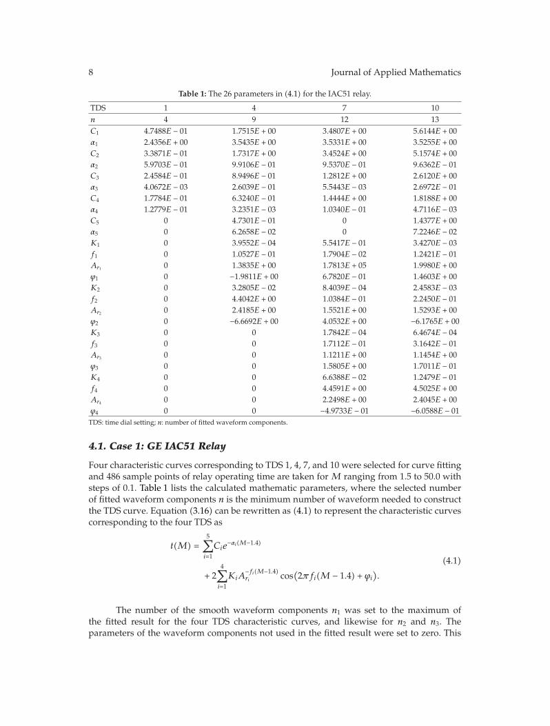
Table 1: The 26 parameters in (4.1) for the IAC51 relay.

TDS 1 4 7 10n 4 9 12 13C1 4.7488E − 01 1.7515E + 00 3.4807E + 00 5.6144E + 00α1 2.4356E + 00 3.5435E + 00 3.5331E + 00 3.5255E + 00C2 3.3871E − 01 1.7317E + 00 3.4524E + 00 5.1574E + 00α2 5.9703E − 01 9.9106E − 01 9.5370E − 01 9.6362E − 01C3 2.4584E − 01 8.9496E − 01 1.2812E + 00 2.6120E + 00α3 4.0672E − 03 2.6039E − 01 5.5443E − 03 2.6972E − 01C4 1.7784E − 01 6.3240E − 01 1.4444E + 00 1.8188E + 00α4 1.2779E − 01 3.2351E − 03 1.0340E − 01 4.7116E − 03C5 0 4.7301E − 01 0 1.4377E + 00α5 0 6.2658E − 02 0 7.2246E − 02K1 0 3.9552E − 04 5.5417E − 01 3.4270E − 03f1 0 1.0527E − 01 1.7904E − 02 1.2421E − 01Ar1 0 1.3835E + 00 1.7813E + 05 1.9980E + 00ϕ1 0 −1.9811E + 00 6.7820E − 01 1.4603E + 00K2 0 3.2805E − 02 8.4039E − 04 2.4583E − 03f2 0 4.4042E + 00 1.0384E − 01 2.2450E − 01Ar2 0 2.4185E + 00 1.5521E + 00 1.5293E + 00ϕ2 0 −6.6692E + 00 4.0532E + 00 −6.1765E + 00K3 0 0 1.7842E − 04 6.4674E − 04f3 0 0 1.7112E − 01 3.1642E − 01Ar3 0 0 1.1211E + 00 1.1454E + 00ϕ3 0 0 1.5805E + 00 1.7011E − 01K4 0 0 6.6388E − 02 1.2479E − 01f4 0 0 4.4591E + 00 4.5025E + 00Ar4 0 0 2.2498E + 00 2.4045E + 00ϕ4 0 0 −4.9733E − 01 −6.0588E − 01TDS: time dial setting; n: number of fitted waveform components.

4.1. Case 1: GE IAC51 Relay

Four characteristic curves corresponding to TDS 1, 4, 7, and 10 were selected for curve fittingand 486 sample points of relay operating time are taken for M ranging from 1.5 to 50.0 withsteps of 0.1. Table 1 lists the calculated mathematic parameters, where the selected numberof fitted waveform components n is the minimum number of waveform needed to constructthe TDS curve. Equation (3.16) can be rewritten as (4.1) to represent the characteristic curvescorresponding to the four TDS as

t(M) =5∑

i=1

Cie−αi(M−1.4)

+ 24∑

i=1

KiA−fi(M−1.4)ri cos

(2πfi(M − 1.4) + ϕi

).

(4.1)

The number of the smooth waveform components n1 was set to the maximum ofthe fitted result for the four TDS characteristic curves, and likewise for n2 and n3. Theparameters of the waveform components not used in the fitted result were set to zero. This


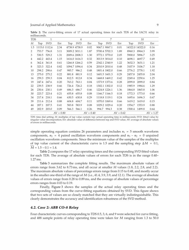
Table 2: The curve-fitting errors of 17 actual operating times for each TDS of the IAC51 relay inmilliseconds.TDS 1 4 7 10M Top SVD Err Top SVD Err Top SVD Err Top SVD Err1.5 1115.0 1112.6 2.34 4738.9 4738.9 0.02 9067.1 9067.1 0.01 14322.0 14322.0 0.162 753.7 756.8 3.11 3009.2 3011.1 1.87 5700.4 5702.3 1.89 8960.3 8964.3 3.993 530.5 529.2 1.31 2009.6 2008.3 1.30 3772.1 3770.0 2.05 5900.0 5896.7 3.254 442.2 443.4 1.15 1616.0 1616.3 0.32 3013.9 3014.0 0.10 4698.1 4697.7 0.496 362.4 361.8 0.61 1266.8 1266.2 0.59 2342.1 2340.9 1.22 3632.3 3631.1 1.218 323.3 322.4 0.82 1094.7 1094.4 0.34 2010.9 2010.4 0.48 3107.9 3106.7 1.1810 298.2 298.6 0.47 985.7 986.2 0.48 1801.4 1802.0 0.66 2776.2 2778.1 1.9213 275.0 275.2 0.22 881.8 881.9 0.12 1601.5 1601.3 0.29 2457.8 2455.8 2.0416 259.3 259.3 0.04 812.5 812.8 0.34 1468.8 1469.2 0.42 2249.4 2250.6 1.2519 247.4 247.6 0.20 763.2 763.1 0.04 1373.9 1373.6 0.28 2099.8 2099.0 0.8422 239.5 238.9 0.66 726.4 726.2 0.18 1302.1 1302.0 0.12 1985.9 1984.6 1.2926 230.6 230.1 0.49 686.3 686.7 0.46 1224.8 1226.1 1.36 1864.8 1865.8 1.0630 223.7 223.4 0.21 655.8 655.8 0.08 1166.7 1166.5 0.18 1772.3 1773.0 0.6634 217.4 218.1 0.66 630.5 630.8 0.29 1118.8 1119.1 0.24 1695.6 1696.3 0.6739 211.6 212.4 0.88 604.8 604.7 0.11 1070.0 1069.4 0.66 1619.2 1619.0 0.1544 207.1 207.5 0.41 583.8 583.9 0.08 1029.2 1029.4 0.20 1554.7 1553.9 0.8849 202.9 203.0 0.09 566.3 566.1 0.26 994.7 994.3 0.38 1500.4 1499.8 0.64

AV = 0.80 AV = 0.40 AV = 0.62 AV = 1.27TDS: time dial setting; M: multiples of tap value current; top: actual operating time in milliseconds; SVD: fitted value bysingular value decomposition; Err: absolute value of difference between top and SVD value; AV: average of absolute valuesof errors in milliseconds.

simple operating equation contains 26 parameters and includes n1 = 5 smooth waveformcomponents, n2 = 4 paired oscillation waveform components and n3 − n2 = 0 unpairedoscillation waveform components. Since the minimum value of the samples of the multiplesof tap value current of the characteristic curve is 1.5 and the sampling step ΔM = 0.1,M = 1.5 − 0.1 = 1.4.

Table 2 compares the 17 relay operating times and the corresponding SVD fitted valuesfor each TDS. The average of absolute values of errors for each TDS is in the range 0.40–1.27ms.

Table 3 summarizes the complete fitting results. The maximum absolute values oferrors range from 3.62 to 8.73ms, and all occur at smaller M values (1.8, 2.2, 2.8, and 2.2).The maximum absolute values of percentage errors range from 0.15 to 0.48, and mostly occurin the smaller one-third of the range ofM (i.e., 41.4, 3.9, 3.9, and 12.1). The average of absolutevalues of errors range from 0.28 to 0.89ms, and the average of absolute values of percentageerrors ranges from 0.03 to 0.19.

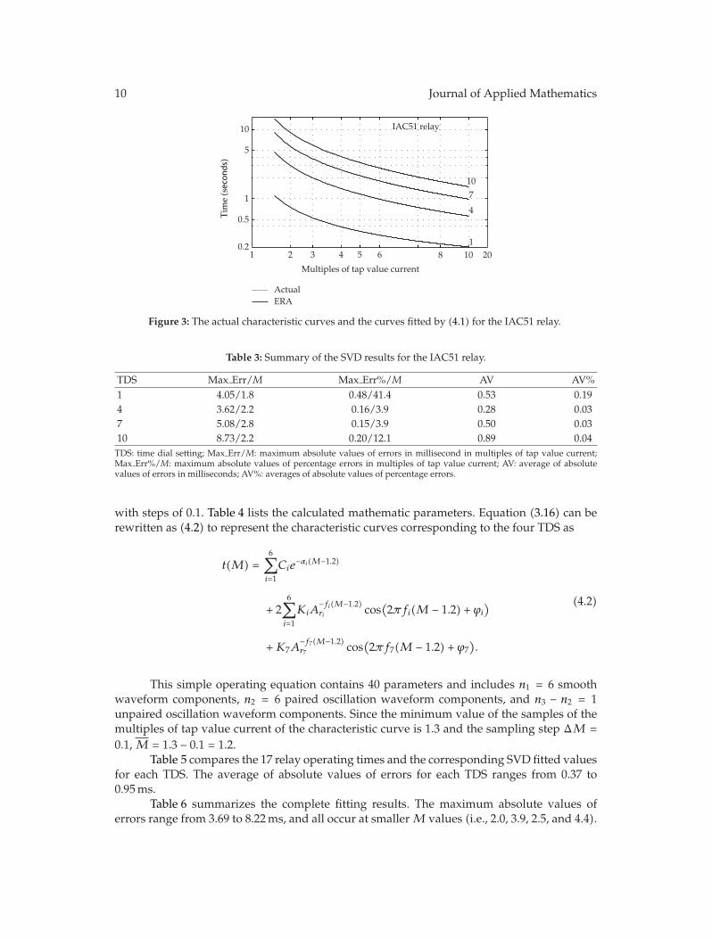
Finally, Figure 3 shows the samples of the actual relay operating times and thecorresponding values from the curve-fitting equations obtained by SVD. This figure showsthat two sets of values are so closely matched that they are virtually indistinguishable. Thisclearly demonstrates the accuracy and identification robustness of the SVD method.

4.2. Case 2: ABB CO-8 Relay

Four characteristic curves corresponding to TDS 0.5, 3, 6, and 9 were selected for curve fitting,and 488 sample points of relay operating time were taken for M ranging from 1.3 to 50.0


1 2 3 4 5 6 8 10 200.2

0.5

1

5

10


ActualERA

4

7

10

1

IAC51 relay

Tim

e(secon

ds)

Figure 3: The actual characteristic curves and the curves fitted by (4.1) for the IAC51 relay.

Table 3: Summary of the SVD results for the IAC51 relay.

TDS Max Err/M Max Err%/M AV AV%1 4.05/1.8 0.48/41.4 0.53 0.194 3.62/2.2 0.16/3.9 0.28 0.037 5.08/2.8 0.15/3.9 0.50 0.0310 8.73/2.2 0.20/12.1 0.89 0.04TDS: time dial setting; Max Err/M: maximum absolute values of errors in millisecond in multiples of tap value current;Max Err%/M: maximum absolute values of percentage errors in multiples of tap value current; AV: average of absolutevalues of errors in milliseconds; AV%: averages of absolute values of percentage errors.

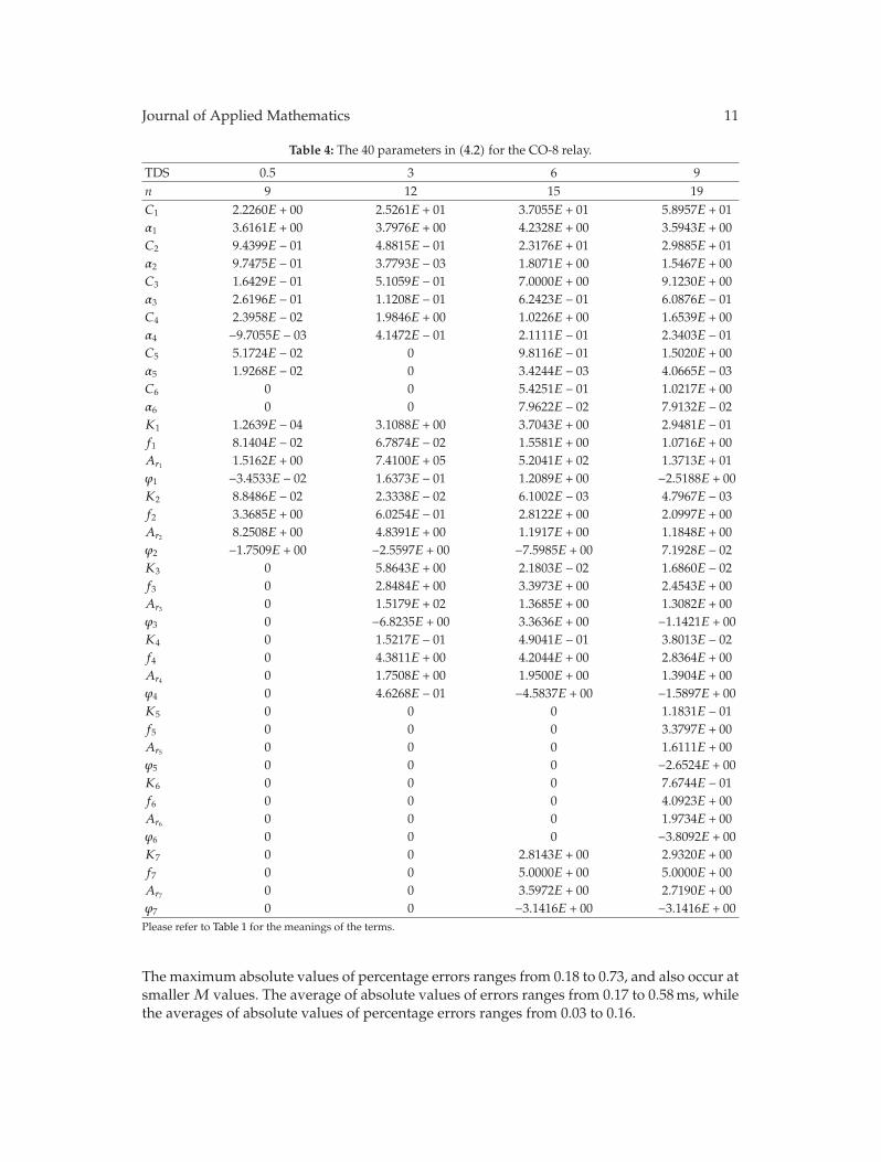
with steps of 0.1. Table 4 lists the calculated mathematic parameters. Equation (3.16) can berewritten as (4.2) to represent the characteristic curves corresponding to the four TDS as

t(M) =6∑

i=1

Cie−αi(M−1.2)

+ 26∑

i=1

KiA−fi(M−1.2)ri cos

(2πfi(M − 1.2) + ϕi

)

+K7A−f7(M−1.2)r7 cos

(2πf7(M − 1.2) + ϕ7

).

(4.2)

This simple operating equation contains 40 parameters and includes n1 = 6 smoothwaveform components, n2 = 6 paired oscillation waveform components, and n3 − n2 = 1unpaired oscillation waveform components. Since the minimum value of the samples of themultiples of tap value current of the characteristic curve is 1.3 and the sampling step ΔM =0.1, M = 1.3 − 0.1 = 1.2.

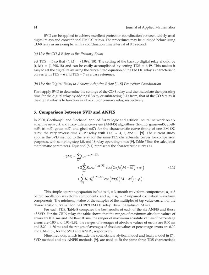
Table 5 compares the 17 relay operating times and the corresponding SVD fitted valuesfor each TDS. The average of absolute values of errors for each TDS ranges from 0.37 to0.95ms.

Table 6 summarizes the complete fitting results. The maximum absolute values oferrors range from 3.69 to 8.22ms, and all occur at smallerM values (i.e., 2.0, 3.9, 2.5, and 4.4).


Table 4: The 40 parameters in (4.2) for the CO-8 relay.

TDS 0.5 3 6 9n 9 12 15 19C1 2.2260E + 00 2.5261E + 01 3.7055E + 01 5.8957E + 01α1 3.6161E + 00 3.7976E + 00 4.2328E + 00 3.5943E + 00C2 9.4399E − 01 4.8815E − 01 2.3176E + 01 2.9885E + 01α2 9.7475E − 01 3.7793E − 03 1.8071E + 00 1.5467E + 00C3 1.6429E − 01 5.1059E − 01 7.0000E + 00 9.1230E + 00α3 2.6196E − 01 1.1208E − 01 6.2423E − 01 6.0876E − 01C4 2.3958E − 02 1.9846E + 00 1.0226E + 00 1.6539E + 00α4 −9.7055E − 03 4.1472E − 01 2.1111E − 01 2.3403E − 01C5 5.1724E − 02 0 9.8116E − 01 1.5020E + 00α5 1.9268E − 02 0 3.4244E − 03 4.0665E − 03C6 0 0 5.4251E − 01 1.0217E + 00α6 0 0 7.9622E − 02 7.9132E − 02K1 1.2639E − 04 3.1088E + 00 3.7043E + 00 2.9481E − 01f1 8.1404E − 02 6.7874E − 02 1.5581E + 00 1.0716E + 00Ar1 1.5162E + 00 7.4100E + 05 5.2041E + 02 1.3713E + 01ϕ1 −3.4533E − 02 1.6373E − 01 1.2089E + 00 −2.5188E + 00K2 8.8486E − 02 2.3338E − 02 6.1002E − 03 4.7967E − 03f2 3.3685E + 00 6.0254E − 01 2.8122E + 00 2.0997E + 00Ar2 8.2508E + 00 4.8391E + 00 1.1917E + 00 1.1848E + 00ϕ2 −1.7509E + 00 −2.5597E + 00 −7.5985E + 00 7.1928E − 02K3 0 5.8643E + 00 2.1803E − 02 1.6860E − 02f3 0 2.8484E + 00 3.3973E + 00 2.4543E + 00Ar3 0 1.5179E + 02 1.3685E + 00 1.3082E + 00ϕ3 0 −6.8235E + 00 3.3636E + 00 −1.1421E + 00K4 0 1.5217E − 01 4.9041E − 01 3.8013E − 02f4 0 4.3811E + 00 4.2044E + 00 2.8364E + 00Ar4 0 1.7508E + 00 1.9500E + 00 1.3904E + 00ϕ4 0 4.6268E − 01 −4.5837E + 00 −1.5897E + 00K5 0 0 0 1.1831E − 01f5 0 0 0 3.3797E + 00Ar5 0 0 0 1.6111E + 00ϕ5 0 0 0 −2.6524E + 00K6 0 0 0 7.6744E − 01f6 0 0 0 4.0923E + 00Ar6 0 0 0 1.9734E + 00ϕ6 0 0 0 −3.8092E + 00K7 0 0 2.8143E + 00 2.9320E + 00f7 0 0 5.0000E + 00 5.0000E + 00Ar7 0 0 3.5972E + 00 2.7190E + 00ϕ7 0 0 −3.1416E + 00 −3.1416E + 00Please refer to Table 1 for the meanings of the terms.

The maximum absolute values of percentage errors ranges from 0.18 to 0.73, and also occur atsmallerM values. The average of absolute values of errors ranges from 0.17 to 0.58ms, whilethe averages of absolute values of percentage errors ranges from 0.03 to 0.16.


Table 5: The curve-fitting errors of 17 actual operating times for each TDS of the CO-8 relay inmilliseconds.

TDS 0.5 3 6 9M Top SVD Err Top SVD Err Top SVD Err Top SVD Err1.5 1682.2 1682.1 0.11 15254.0 15254.0 0.10 31907.0 31907.0 0.26 50681.0 50681.0 0.162 760.5 764.2 3.69 6182.1 6182.6 0.49 13232.0 13232.0 0.21 21256.0 21257.0 1.113 343.9 343.6 0.25 2577.6 2581.6 3.98 5334.0 5337.1 3.10 8449.4 8450.2 0.784 213.7 214.3 0.60 1578.5 1578.0 0.44 3341.9 3339.4 2.51 5222.6 5218.7 3.926 128.1 127.6 0.55 1004.0 1002.7 1.24 2062.6 2060.3 2.32 3221.3 3218.3 3.028 99.7 99.7 0.01 821.3 820.2 1.12 1618.9 1618.4 0.44 2542.7 2540.0 2.6610 86.1 86.3 0.19 711.7 712.9 1.13 1407.3 1409.4 2.16 2210.1 2211.9 1.7913 75.8 75.7 0.04 618.3 617.9 0.42 1244.0 1243.5 0.56 1944.8 1944.7 0.1016 70.1 70.0 0.10 563.1 563.1 0.01 1145.0 1145.3 0.30 1783.3 1783.9 0.6219 66.5 66.6 0.13 526.5 527.1 0.56 1078.3 1078.6 0.28 1672.8 1672.7 0.0622 64.7 64.6 0.07 501.4 501.2 0.12 1030.0 1029.9 0.06 1589.8 1589.9 0.1326 62.9 62.9 0.01 476.0 476.2 0.23 982.0 982.0 0.02 1506.4 1506.5 0.0230 61.4 61.4 0.00 458.5 458.1 0.47 946.5 946.1 0.36 1442.9 1442.6 0.3334 60.1 60.4 0.35 443.7 444.2 0.45 917.4 917.8 0.38 1390.5 1391.4 0.9339 59.6 59.6 0.02 430.7 430.6 0.19 889.1 889.1 0.02 1339.7 1339.5 0.1444 59.0 58.9 0.09 419.3 419.5 0.20 865.5 865.5 0.03 1297.0 1296.7 0.2749 58.6 58.7 0.12 409.8 409.9 0.11 845.0 845.1 0.14 1260.1 1259.9 0.15

AV = 0.37 AV = 0.66 AV = 0.77 AV = 0.95Please refer to Table 2 for the meanings of the terms.

Table 6: Summary of the SVD results for the CO-8 relay.

TDS Max Err/M Max Err%/M AV AV%0.5 3.69/2.0 0.73/3.9 0.17 0.163 8.22/3.9 0.50/3.9 0.42 0.056 7.72/2.5 0.29/5.2 0.53 0.039 6.08/4.4 0.18/6.9 0.58 0.03Please refer to Table 3 for the meanings of the terms.

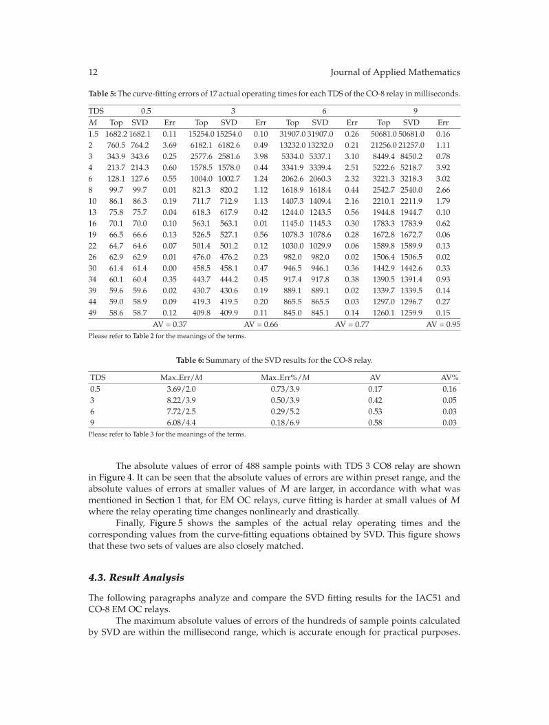
The absolute values of error of 488 sample points with TDS 3 CO8 relay are shownin Figure 4. It can be seen that the absolute values of errors are within preset range, and theabsolute values of errors at smaller values of M are larger, in accordance with what wasmentioned in Section 1 that, for EM OC relays, curve fitting is harder at small values of Mwhere the relay operating time changes nonlinearly and drastically.

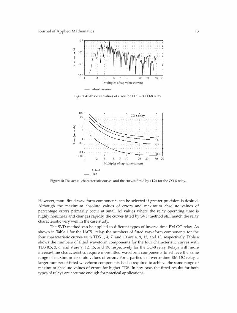
Finally, Figure 5 shows the samples of the actual relay operating times and thecorresponding values from the curve-fitting equations obtained by SVD. This figure showsthat these two sets of values are also closely matched.

4.3. Result Analysis

The following paragraphs analyze and compare the SVD fitting results for the IAC51 andCO-8 EM OC relays.

The maximum absolute values of errors of the hundreds of sample points calculatedby SVD are within the millisecond range, which is accurate enough for practical purposes.


1 2 3 5 7 10 20 30 50 70


Absolute error

10−5

10−4

10−3

10−2

Tim

e(secon

ds)

Figure 4: Absolute values of error for TDS = 3 CO-8 relay.

1 2 3 5 7 10 20 30 50 700.050.1

0.51

510

50100


369

0.5

ActualERA

CO-8 relay

Tim

e(secon

ds)

Figure 5: The actual characteristic curves and the curves fitted by (4.2) for the CO-8 relay.

However, more fitted waveform components can be selected if greater precision is desired.Although the maximum absolute values of errors and maximum absolute values ofpercentage errors primarily occur at small M values where the relay operating time ishighly nonlinear and changes rapidly, the curves fitted by SVD method still match the relaycharacteristic very well in the case study.

The SVD method can be applied to different types of inverse-time EM OC relay. Asshown in Table 1 for the IAC51 relay, the numbers of fitted waveform components for thefour characteristic curves with TDS 1, 4, 7, and 10 are 4, 9, 12, and 13, respectively. Table 4shows the numbers of fitted waveform components for the four characteristic curves withTDS 0.5, 3, 6, and 9 are 9, 12, 15, and 19, respectively for the CO-8 relay. Relays with moreinverse-time characteristics require more fitted waveform components to achieve the samerange of maximum absolute values of errors. For a particular inverse-time EM OC relay, alarger number of fitted waveform components is also required to achieve the same range ofmaximum absolute values of errors for higher TDS. In any case, the fitted results for bothtypes of relays are accurate enough for practical applications.


SVD can be applied to achieve excellent protection coordination between widely useddigital relays and conventional EM OC relays. The procedures may be outlined below usingCO-8 relay as an example, with a coordination time interval of 0.3 second.

(a) Use the CO-8 Relay as the Primary Relay

Set TDS = 5 so that (t, M) = (1.098, 18). The setting of the backup digital relay should be(t,M) = (1.398, 18) and can be easily accomplished by setting TDS = 6.49. This makes iteasy to set the digital relay using the curve-fitted equation of the EMOC relay’s characteristiccurves with TDS = 6 and TDS = 7 as a base reference.

(b) Use the Digital Relay to Achieve Adaptive Relay [1, 8] Protection Coordination

First, apply SVD to determine the settings of the CO-8 relay and then calculate the operatingtime for the digital relay by adding 0.3 s to, or subtracting 0.3 s from, that of the CO-8 relay ifthe digital relay is to function as a backup or primary relay, respectively.

5. Comparison between SVD and ANFIS

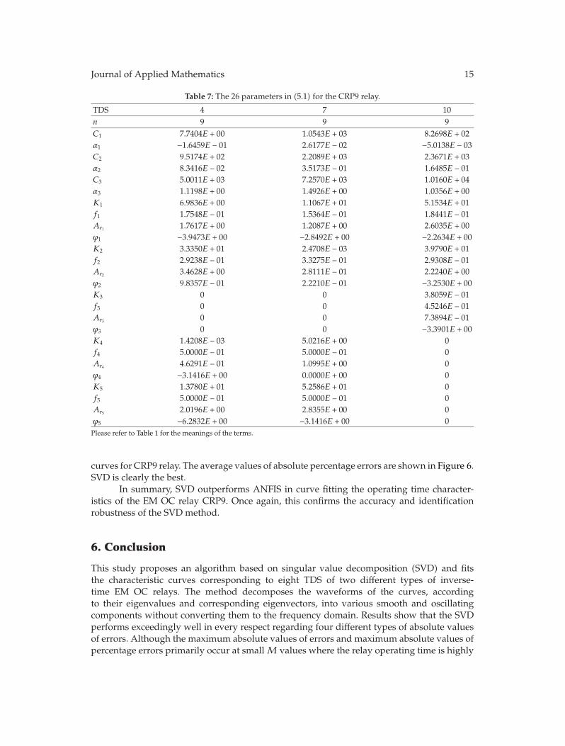
In 2008, Geethanjali and Slochanal applied fuzzy logic and artificial neural network on sixadaptive network and fuzzy inference system (ANFIS) algorithms (tri-mf5, gauss-mf5, gbell-mf5, tri-mf7, gauss-mf7, and gbell-mf7) for the characteristic curve fitting of one EM OCrelay: the very inverse-time CRP9 relay with TDS = 4, 7, and 10 [9]. The current studyapplies the SVD method to the relay for the same TDS characteristic curves for comparisonpurposes, with sampling step 1.0, and 18 relay operating times [9]. Table 7 lists the calculatedmathematic parameters. Equation (5.1) represents the characteristic curves as

t(M) =3∑

i=1

Cie−αi(M−M)

+ 23∑

i=1


(2πfi

(M −M

)+ ϕi

)

+5∑

i=4


(2πfi

(M −M

)+ ϕi

).

(5.1)

This simple operating equation includes n1 = 3 smooth waveform components, n2 = 3paired oscillation waveform components, and n3 − n2 = 2 unpaired oscillation waveformcomponents. The minimum value of the samples of the multiples of tap value current of thecharacteristic curve is 3 for the CRP9 EM OC relay. Thus, the value ofM is 2.

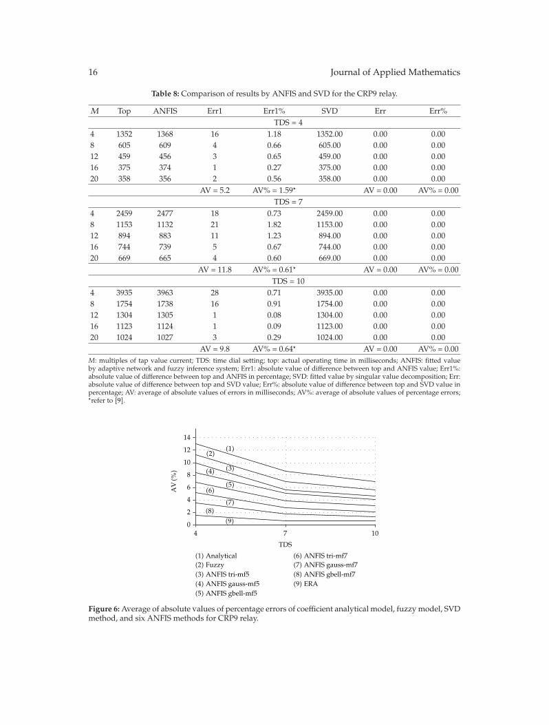
For each TDS, Table 8 compares the best results of each of the six ANFIS and thoseof SVD. For the CRP9 relay, the table shows that the ranges of maximum absolute values oferrors are 0.00ms and 16.00–28.00ms, the ranges of maximum absolute values of percentageerrors are 0.00 and 0.91–1.82, the ranges of averages of absolute values of errors are 0.00msand 5.20–11.80ms and the ranges of averages of absolute values of percentage errors are 0.00and 0.61–1.59, for the SVD and ANFIS, respectively.

Nine methods, which include the coefficient analytical model and fuzzy model in [7],SVD method and six ANFIS methods [9], are used to fit the same three TDS characteristic


Table 7: The 26 parameters in (5.1) for the CRP9 relay.

TDS 4 7 10n 9 9 9C1 7.7404E + 00 1.0543E + 03 8.2698E + 02α1 −1.6459E − 01 2.6177E − 02 −5.0138E − 03C2 9.5174E + 02 2.2089E + 03 2.3671E + 03α2 8.3416E − 02 3.5173E − 01 1.6485E − 01C3 5.0011E + 03 7.2570E + 03 1.0160E + 04α3 1.1198E + 00 1.4926E + 00 1.0356E + 00K1 6.9836E + 00 1.1067E + 01 5.1534E + 01f1 1.7548E − 01 1.5364E − 01 1.8441E − 01Ar1 1.7617E + 00 1.2087E + 00 2.6035E + 00ϕ1 −3.9473E + 00 −2.8492E + 00 −2.2634E + 00K2 3.3350E + 01 2.4708E − 03 3.9790E + 01f2 2.9238E − 01 3.3275E − 01 2.9308E − 01Ar2 3.4628E + 00 2.8111E − 01 2.2240E + 00ϕ2 9.8357E − 01 2.2210E − 01 −3.2530E + 00K3 0 0 3.8059E − 01f3 0 0 4.5246E − 01Ar3 0 0 7.3894E − 01ϕ3 0 0 −3.3901E + 00K4 1.4208E − 03 5.0216E + 00 0f4 5.0000E − 01 5.0000E − 01 0Ar4 4.6291E − 01 1.0995E + 00 0ϕ4 −3.1416E + 00 0.0000E + 00 0K5 1.3780E + 01 5.2586E + 01 0f5 5.0000E − 01 5.0000E − 01 0Ar5 2.0196E + 00 2.8355E + 00 0ϕ5 −6.2832E + 00 −3.1416E + 00 0Please refer to Table 1 for the meanings of the terms.

curves for CRP9 relay. The average values of absolute percentage errors are shown in Figure 6.SVD is clearly the best.

In summary, SVD outperforms ANFIS in curve fitting the operating time character-istics of the EM OC relay CRP9. Once again, this confirms the accuracy and identificationrobustness of the SVD method.

6. Conclusion

This study proposes an algorithm based on singular value decomposition (SVD) and fitsthe characteristic curves corresponding to eight TDS of two different types of inverse-time EM OC relays. The method decomposes the waveforms of the curves, accordingto their eigenvalues and corresponding eigenvectors, into various smooth and oscillatingcomponents without converting them to the frequency domain. Results show that the SVDperforms exceedingly well in every respect regarding four different types of absolute valuesof errors. Although the maximum absolute values of errors and maximum absolute values ofpercentage errors primarily occur at smallM values where the relay operating time is highly


Table 8: Comparison of results by ANFIS and SVD for the CRP9 relay.

M Top ANFIS Err1 Err1% SVD Err Err%TDS = 4

4 1352 1368 16 1.18 1352.00 0.00 0.008 605 609 4 0.66 605.00 0.00 0.0012 459 456 3 0.65 459.00 0.00 0.0016 375 374 1 0.27 375.00 0.00 0.0020 358 356 2 0.56 358.00 0.00 0.00

AV = 5.2 AV% = 1.59� AV = 0.00 AV% = 0.00TDS = 7

4 2459 2477 18 0.73 2459.00 0.00 0.008 1153 1132 21 1.82 1153.00 0.00 0.0012 894 883 11 1.23 894.00 0.00 0.0016 744 739 5 0.67 744.00 0.00 0.0020 669 665 4 0.60 669.00 0.00 0.00

AV = 11.8 AV% = 0.61� AV = 0.00 AV% = 0.00TDS = 10

4 3935 3963 28 0.71 3935.00 0.00 0.008 1754 1738 16 0.91 1754.00 0.00 0.0012 1304 1305 1 0.08 1304.00 0.00 0.0016 1123 1124 1 0.09 1123.00 0.00 0.0020 1024 1027 3 0.29 1024.00 0.00 0.00

AV = 9.8 AV% = 0.64� AV = 0.00 AV% = 0.00M: multiples of tap value current; TDS: time dial setting; top: actual operating time in milliseconds; ANFIS: fitted valueby adaptive network and fuzzy inference system; Err1: absolute value of difference between top and ANFIS value; Err1%:absolute value of difference between top and ANFIS in percentage; SVD: fitted value by singular value decomposition; Err:absolute value of difference between top and SVD value; Err%: absolute value of difference between top and SVD value inpercentage; AV: average of absolute values of errors in milliseconds; AV%: average of absolute values of percentage errors;�refer to [9].

4

14

10

8

6

2

4 7 100

12

TDS

(1) Analytical(2) Fuzzy(3) ANFIS tri-mf5(4) ANFIS gauss-mf5(5) ANFIS gbell-mf5

(6) ANFIS tri-mf7(7) ANFIS gauss-mf7(8) ANFIS gbell-mf7(9) ERA

AV(%

)

(2)(1)

(3)(4)

(5)(6)

(7)(8)

(9)

Figure 6:Average of absolute values of percentage errors of coefficient analytical model, fuzzy model, SVDmethod, and six ANFIS methods for CRP9 relay.


nonlinear and changes rapidly, the curves fitted by the SVD method can still match the relaycharacteristic very well. The SVD is also superior to ANFIS.

The ability to accurately represent the characteristic curves of the EM OC relaysby a simple equation can provide good protection coordination between conventional EMOC relays and digital relays for subtransmission systems and distribution systems. Theformula is a unified equation by SVD algorithm, and it can fit the characteristics of anypiecewise nonlinear continuous smooth descending curves by simply changing the values ofits parameters. Such convenience or advantage can be exploited not only for OC protectionequipments such as EMOC relays or power fuses in power systems for practical applicationsor future studies, but also for any subject in any field with such characteristic.

References

[1] A. Conde and E. Vazquez, “Application of a proposed overcurrent relay in radial distributionnetworks,” Electric Power Systems Research, vol. 81, no. 2, pp. 570–579, 2011.

[2] M. S. Sachdev, J. Singh, and R. J. Fleming, “Mathematical models representing time-currentcharacteristics of overcurrent relays for computer applications,” in Proceedings of the IEEE Power &Energy Society, no. Paper No. A78-131-5, January 1978.

[3] IEEE Committee Report, “Computer representation of overcurrent relay characteristics,” IEEETransactions on Power Delivery, vol. 4, no. 3, pp. 1659–1667, 1989.

[4] S. Chan and R. Maurer, “Modeling overcurrent relay characteristics,” IEEE Computer Applications inPower, vol. 5, no. 1, pp. 41–45, 1992.

[5] IEEE PSRC Committee, “IEEE standard inverse-time characteristic equations for overcurrent relays,”IEEE Transactoions on Power Delivery, vol. 14, no. 3, pp. 868–872, 1999.

[6] D. J. Hill, L. W. Bruehler, and C. J. Bohrer, “Why wait? System-wide benefits from custom overcurrentrelay characteristics,” in Proceedings of the 56th Annual Petroleum and Chemical Industry Conference (PCIC’09), pp. 1–9, September 2009.

[7] K. K. Hossein, A. A. Hossein, and A. D. Majid, “A flexible approach for overcurrent relaycharacteristics simulation,” Electric Power Systems Research, vol. 66, no. 3, pp. 233–239, 2003.

[8] C. E. Arturo, V. M. Ernesto, and J. A. Hector, “Time overcurrent adaptive relay,” International Journalof Electrical Power and Energy System, vol. 25, no. 10, pp. 841–847, 2003.

[9] M. Geethanjali and S. M. R. Slochanal, “A combined adaptive network and fuzzy inference system(ANFIS) approach for overcurrent relay system,” Neurocomputing, vol. 71, no. 4–6, pp. 895–903, 2008.

[10] H. A. Darwish, M. A. Rahman, A. I. Taalab, and H. Shaaban, “Digital model of overcurrent relaycharacteristics,” in Proceedings of the Conference Record of the IEEE Industry Applications 30th IAS AnnualMeeting, pp. 1187–1192, October 1995.

[11] B. Yan, X. Xie, and Q. Jiang, “Principal Hankel Component Algorithm (PHCA) for power systemidentification,” in Proceedings of the IEEE/PES Power Systems Conference and Exposition (PSCE ’09), pp.1–5, March 2009.

[12] J. S. H. Tsai, T. H. Chien, S. M. Guo, Y. P. Chang, and L. S. Shieh, “State-space self-tuning control forstochastic fractional-order chaotic systems,” IEEE Transactions on Circuits and Systems, vol. 54, no. 3,pp. 632–642, 2007.

[13] S. M. Djouadi, R. C. Camphouse, and J. H. Myatt, “Reduced order models for boundary feedbackflow control,” in Proceedings of the American Control Conference (ACC ’08), pp. 4005–4010, June 2008.

[14] Z.Ma, S. Ahuja, and C.W. Rowley, “Reduced-ordermodels for control of fluids using the eigensystemrealization algorithm,” Theoretical and Computational Fluid Dynamics, vol. 25, no. 1–4, pp. 233–247, 2011.

[15] X. D. Sun, T. Clarke, and M. A. Maiza, “A toolbox for minimal state space model realization,” inProceedings of the IEE of Control Theory Application, vol. 143, pp. 152–158, 1996.

[16] J. C. Tan, P. G. McLaren, R. P. Jayasinghe, and P. L. Wilson, “Software model for inverse timeovercurrent relays incorporating IEC and IEEE standard curves,” in Proceedings of the IEEE CanadianConference on Electrical and Computer Engineering, vol. 1, pp. 37–41, May 2002.

[17] IEC Publication 255-3 (1989-05), Single input energizing quality measuring relays with dependent orindependent.

[18] T. H. Tan and G. H. Tzeng, Industry Power Distribution, Gau Lih Book, 4th edition, 2011.[19] BE1-1051 Manual, Basler Electric.


[20] J. N. Juang, Applied System Identification, Prentice Hall, Englewood Cliffs, NJ, USA, 1994.[21] J. T. Kuan and M. K. Chen, “Parameter evaluation for lightning impulse with oscillation and

overshoot using the eigensystem realization algorithm,” IEEE Transactions on Dielectrics and ElectricalInsulation, vol. 13, no. 6, pp. 1303–1316, 2006.

[22] Instructions GEK-49821F, Phase Directional Overcurrent Relays, General Electric, Ontario, Canada, 1999.

Submit your manuscripts athttp://www.hindawi.com

Hindawi Publishing Corporationhttp://www.hindawi.com Volume 2014

MathematicsJournal of


Mathematical Problems in Engineering

Hindawi Publishing Corporationhttp://www.hindawi.com

Differential EquationsInternational Journal of

Volume 2014

Applied MathematicsJournal of


Probability and StatisticsHindawi Publishing Corporationhttp://www.hindawi.com Volume 2014

Journal of


Mathematical PhysicsAdvances in

Complex AnalysisJournal of


OptimizationJournal of


CombinatoricsHindawi Publishing Corporationhttp://www.hindawi.com Volume 2014

International Journal of


Operations ResearchAdvances in

Journal of


Function Spaces

Abstract and Applied AnalysisHindawi Publishing Corporationhttp://www.hindawi.com Volume 2014

International Journal of Mathematics and Mathematical Sciences


The Scientific World JournalHindawi Publishing Corporation http://www.hindawi.com Volume 2014


Algebra

Discrete Dynamics in Nature and Society



Decision SciencesAdvances in

Discrete MathematicsJournal of

Hindawi Publishing Corporationhttp://www.hindawi.com

Volume 2014 Hindawi Publishing Corporationhttp://www.hindawi.com Volume 2014

Stochastic AnalysisInternational Journal of

Documents

Modeling Electromechanical Overcurrent Relays Using ...downloads.hindawi.com/journals/jam/2012/104952.pdf · some older relays have been replaced by new digital ones, there are still