Modeling clustered survival data The different approaches

Modeling clustered Modeling clustered survival datasurvival data

The different approachesThe different approaches

Alternative approaches for Alternative approaches for modeling clustered survival modeling clustered survival

datadata The fixed effects modelThe fixed effects model The stratified modelThe stratified model The frailty modelThe frailty model The marginal modelThe marginal model

Example of bivariate survival Example of bivariate survival datadata

Time to reconstitution of blood-milk Time to reconstitution of blood-milk barrier after mastitisbarrier after mastitis Two quarters are infected with E. coli One quarter treated locally, other quarter

not Blood milk-barrier destroyed Milk Na+ increases Time to normal Na+ level

Time to reconstitution dataTime to reconstitution data

Cow number 1 2 3 … 99 100

Heifer 1 1 0 … 1 0

Treatment 1.9 6.50* 4.78 … 0.66 4.93

Placebo 0.41 6.50* 2.62 … 0.98 6.50*

Time to reconstitution Time to reconstitution figurativefigurative

Cow number

Tim

e t

o r

eso

lutio

n

0 20 40 60 80 100

01

23

45

6

The parametric fixed effects The parametric fixed effects modelmodel

Introduce fixed cow effectIntroduce fixed cow effect

We parameterise baseline hazard We parameterise baseline hazard E.g. Weibull: E.g. Weibull:

iijij cxthth exp)()( 0

Baseline hazard Treatment effect

Fixed cow effect,c1=0

,ith w)( 10 tth

The proportional hazards The proportional hazards modelmodel

From the modelFrom the model

it follows that the hazard ratio of two it follows that the hazard ratio of two individuals is given byindividuals is given by

and this ratio is thus constant over timeand this ratio is thus constant over time


kxl

iij

kl

ij

cxth

cxth

th

th

exp)(

exp)(

)(

)(

0

0

Fixed effects model Fixed effects model likelihoodlikelihood

Survival likelihood: hazard and survival functions Survival likelihood: hazard and survival functions requiredrequired

Maximise log likelihood to find estimates for Maximise log likelihood to find estimates for , , ccii

and and

iijiij

t

ij cxtHcxthtS

exp)(expexp)(exp)( 00 0

)(log)(log )()(1

2

11

2

1

s

i jijijijfixij

s

i jijfix tSthltSthL ij


Parameter estimatesParameter estimatesfixed effects modelfixed effects model

Parameter estimate for trt effect Parameter estimate for trt effect with with =1=1

Additionally another 99 (!) parameters for Additionally another 99 (!) parameters for the different cowsthe different cows

ModelModel SE(SE())

Fixed effectsFixed effects 0.1850.185 0.1900.190

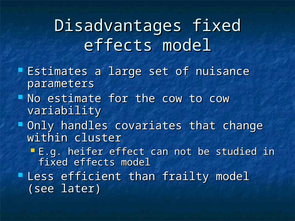
Disadvantages fixed effects Disadvantages fixed effects modelmodel

Estimates a large set of nuisance Estimates a large set of nuisance parametersparameters

No estimate for the cow to cow variabilityNo estimate for the cow to cow variability Only handles covariates that change Only handles covariates that change

within clusterwithin cluster E.g. heifer effect can not be studied in fixed E.g. heifer effect can not be studied in fixed

effects modeleffects model Less efficient than frailty model (see Less efficient than frailty model (see

later)later)

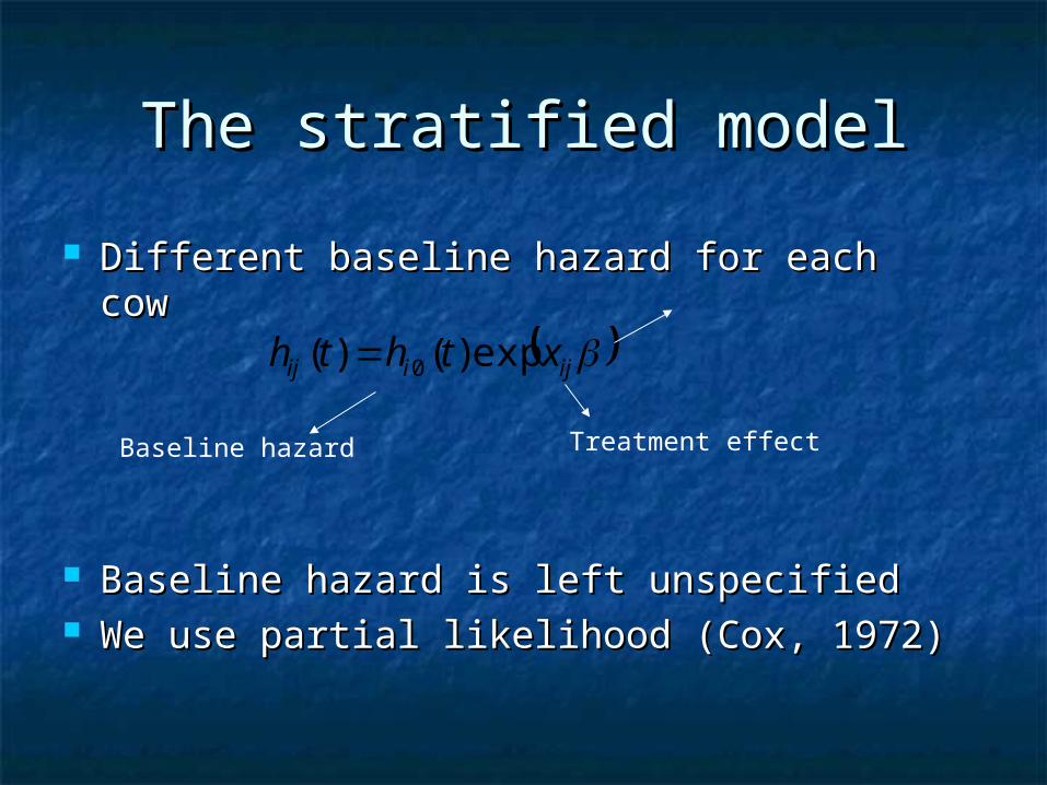
The stratified modelThe stratified model

Different baseline hazard for each cowDifferent baseline hazard for each cow

Baseline hazard is left unspecifiedBaseline hazard is left unspecified We use partial likelihood (Cox, 1972)We use partial likelihood (Cox, 1972)

ijiij xthth exp)()( 0

Baseline hazard Treatment effect

Stratified model likelihoodStratified model likelihood

Partial likelihood determined for each cow Partial likelihood determined for each cow separately, then multiplied (independence)separately, then multiplied (independence)

Maximise partial log likelihood to find Maximise partial log likelihood to find estimates for estimates for alone alone

s

i j yRl il

ij

ij

ijix

x

1

2

1 exp

exp

ijiliji yylyR :

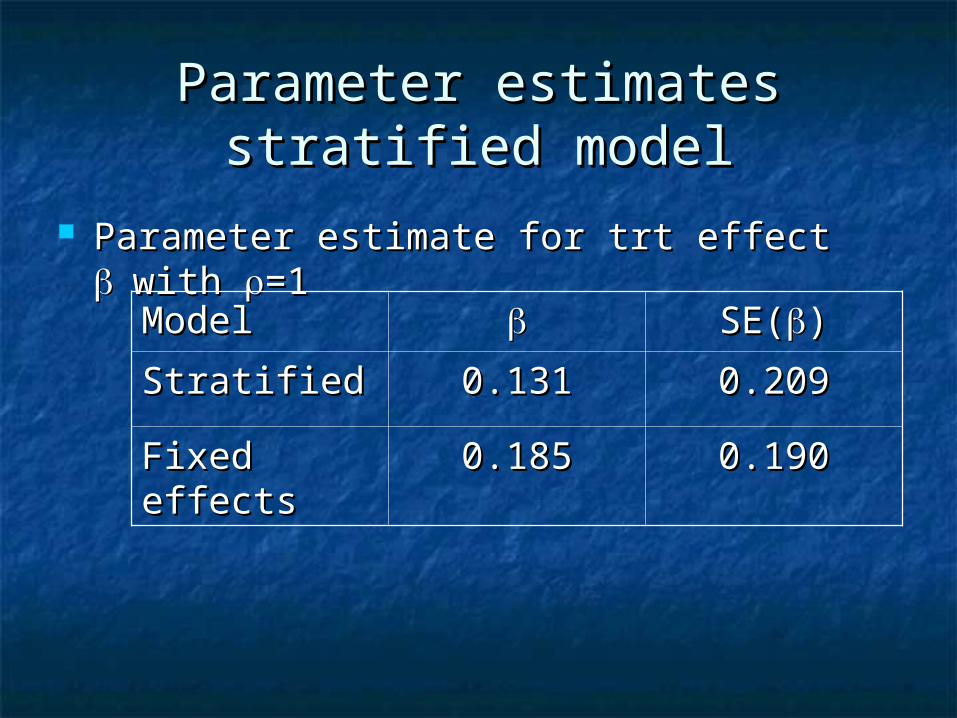
Parameter estimatesParameter estimatesstratified modelstratified model


ModelModel SE(SE())

StratifiedStratified 0.1310.131 0.2090.209


Disadvantages stratified Disadvantages stratified modelmodel

=disadvantages fixed effects model=disadvantages fixed effects model Even more inefficientEven more inefficient

A cow only contributes to the partial A cow only contributes to the partial likelihood if an event is observed for one likelihood if an event is observed for one quarter while the other quarter is still at quarter while the other quarter is still at risk risk

s

i j ii

iiiiii

xx

yyxyyx ii

1

2

1 21

122211

expexp

exp exp 21

11

The frailty modelThe frailty model Different frailty term for each cowDifferent frailty term for each cow

Baseline hazard is assumed to be Baseline hazard is assumed to be parametricparametric

We make distributional assumptions for We make distributional assumptions for uuii

E.g. one parameter gamma frailty densityE.g. one parameter gamma frailty density

ijiij xuthth exp )()( 0

Baseline hazard

Treatment effect

Random cow effect

1

exp1

11

iiiU

uuuf

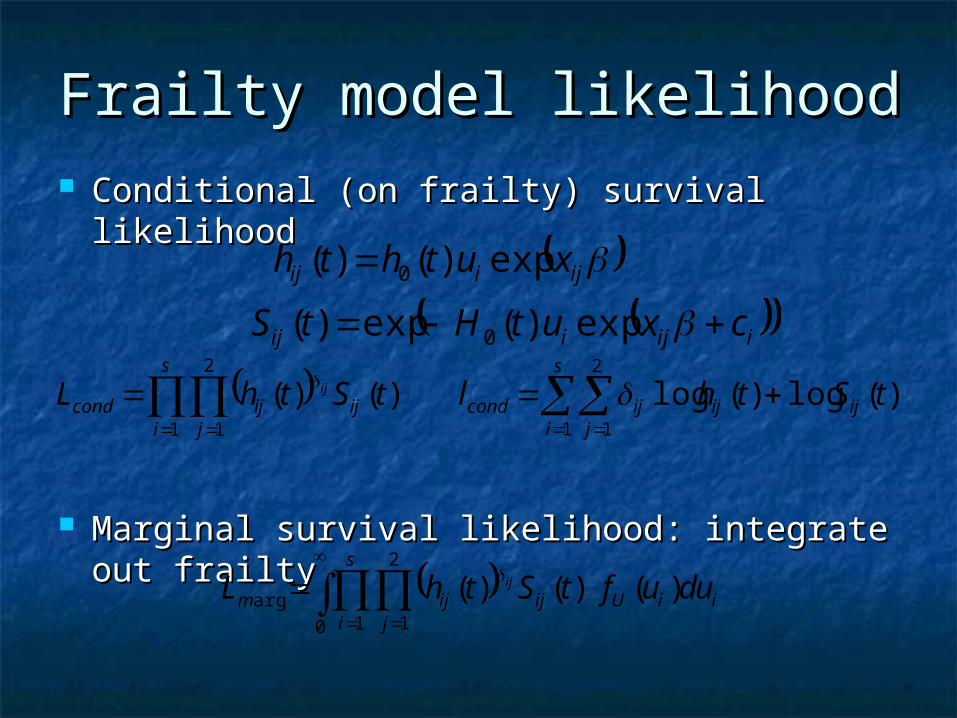
Frailty model likelihoodFrailty model likelihood Conditional (on frailty) survival likelihoodConditional (on frailty) survival likelihood

Marginal survival likelihood: integrate out Marginal survival likelihood: integrate out frailty frailty

iijiij cxutHtS exp )(exp)( 0

)(log)(log )()(1

2

11

2

1

s

i jijijijcondij

s

i jijcond tSthltSthL ij

ijiij xuthth exp )()( 0

iiUij

s

i jijm uduftSthL ij

0 1

2

1arg )( )()(

Parameter estimatesParameter estimatesfrailty modelfrailty model


ModelModel SE(SE())

FrailtyFrailty 0.1710.171 0.1680.168



Advantages frailty modelAdvantages frailty model Provides an estimate of the cow to cow Provides an estimate of the cow to cow

variability, variability, or the variance of the random or the variance of the random effect.effect. In our example, In our example, =0.286 =0.286

It will also give estimates for covariates that are It will also give estimates for covariates that are only changing from cluster to cluster, only changing from cluster to cluster, E.g. the heifer variable changes from cow to cow E.g. the heifer variable changes from cow to cow

It uses the available information in the most It uses the available information in the most efficient wayefficient way It uses all information, even if within a cluster one It uses all information, even if within a cluster one

observation is missingobservation is missing Most efficient even for balanced bivariate survival dataMost efficient even for balanced bivariate survival data

Undadjusted modelUndadjusted model Finally consider unadjusted modelFinally consider unadjusted model

Are observed results for our example Are observed results for our example coincidence or do they reflect a particular coincidence or do they reflect a particular pattern?pattern?

ijij xthth exp)()( 0

ModelModel SE(SE())

UnadjustedUnadjusted 0.1760.176 0.1620.162

FrailtyFrailty 0.1710.171 0.1680.168



Asymptotic varianceAsymptotic variance

The asymptotic variance of the estimate of The asymptotic variance of the estimate of is given as a diagonal element of the is given as a diagonal element of the inverse of observed or expected inverse of observed or expected information matrixinformation matrix

The expected (Fisher) information matrix isThe expected (Fisher) information matrix is

with with HH(() the Hessian matrix () the Hessian matrix ( is parameter is parameter vector)vector)

with (q,r)with (q,r)thth element element

ςHς E)( I

)( 2

ςlrq

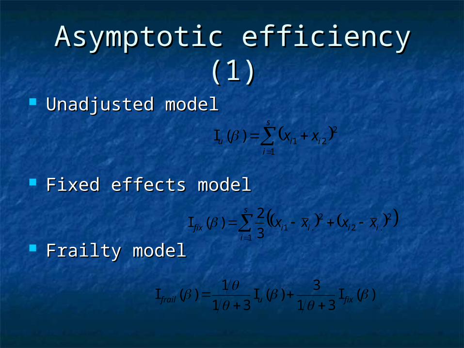
Asymptotic efficiency (1)Asymptotic efficiency (1)

Unadjusted modelUnadjusted model

Fixed effects modelFixed effects model

Frailty modelFrailty model

s

iiiu xx

1

221)(I

s

iiiiifix xxxx

1

2.2

2.13

2)(I

)(I31

3)(I

31

1)(I

fixufrail

Asymptotic efficiency (2)Asymptotic efficiency (2)C

on

trib

utio

n u

na

dju

ste

d m

od

el

0 1 2 3 4

0.0

0.2

0.4

0.6

0.8

1.0

0.33

0.5

Small sample size efficiency by Small sample size efficiency by simulationsimulation

Generate 2000 data sets with 100 Generate 2000 data sets with 100 pairs of two subjects with pairs of two subjects with =0.23, =0.23, =0.18, =0.18, =0.3=0.3

Three different settingsThree different settings 100 % balance100 % balance 80 % balance80 % balance 80 % uncensored80 % uncensored

Look at median and coverageLook at median and coverage

Simulation resultsSimulation results

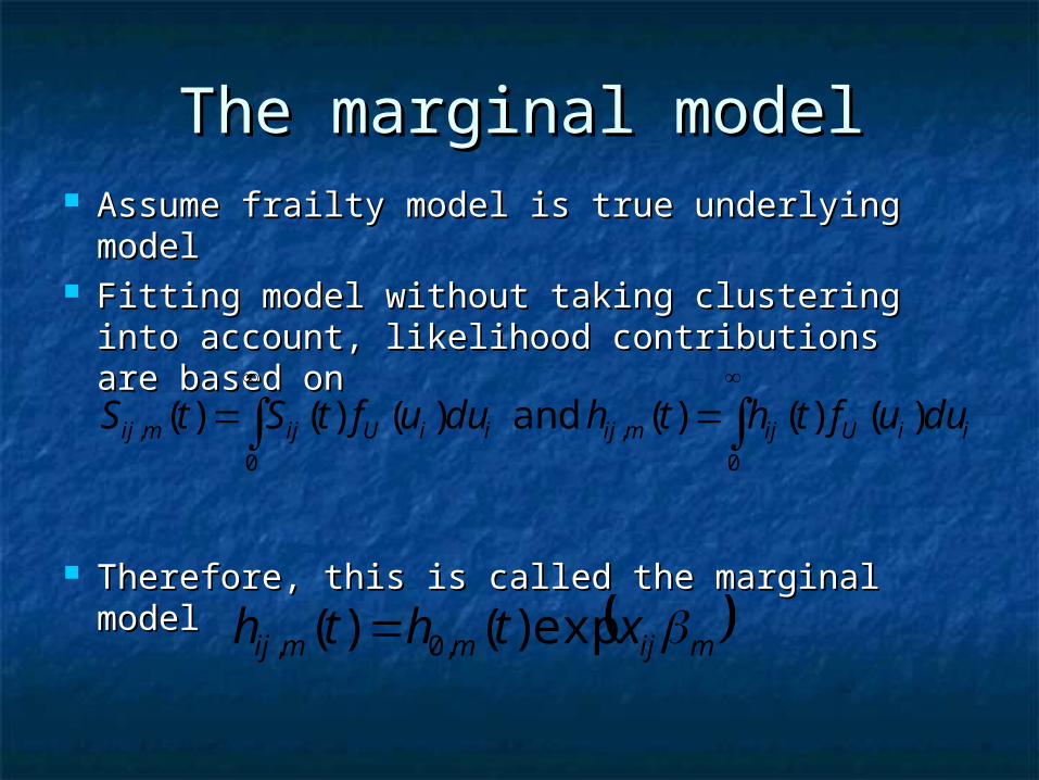
The marginal modelThe marginal model Assume frailty model is true underlying Assume frailty model is true underlying

modelmodel Fitting model without taking clustering into Fitting model without taking clustering into

account, likelihood contributions are based account, likelihood contributions are based onon

Therefore, this is called the marginal modelTherefore, this is called the marginal model mijmmij xthth exp)()( ,0,

)()()( and )()()(0

,

0

,

iiUijmijiiUijmij duufththduuftStS

Marginal model parameter Marginal model parameter estimatesestimates

The estimate is a consistent estimator The estimate is a consistent estimator for for See Wei, Lin and Weissfeld (1989) See Wei, Lin and Weissfeld (1989)

Its asymptotic variance might not be Its asymptotic variance might not be correct because no adjustment done for correct because no adjustment done for correlationcorrelation

We might use eitherWe might use either Jackknife estimatorsJackknife estimators Sandwich estimators Sandwich estimators

m̂

Jackknife estimatorJackknife estimator Generally given byGenerally given by

We use grouped jackknife techniqueWe use grouped jackknife technique Left-out observations independent of Left-out observations independent of

remainingremaining

N

i

T

iiN

pN

1

ˆˆˆˆ ββββ

s

i

T

iis

ps

1

ˆˆˆˆ ββββ

Jackknife versus sandwichJackknife versus sandwich Lipsitz (1994) demonstrates Lipsitz (1994) demonstrates

correspondence between jaccknife correspondence between jaccknife and sandwich estimatorand sandwich estimator

In the time to blood milk In the time to blood milk reconstitutionreconstitution Unadjusted model: SE = 0.176Unadjusted model: SE = 0.176 Grouped jackknife estimator: SE = 0.153Grouped jackknife estimator: SE = 0.153

Grouped jackknife estimator leads to Grouped jackknife estimator leads to smaller variance!! Is this always so?smaller variance!! Is this always so?

Simulation resultsSimulation resultsjackknifejackknife

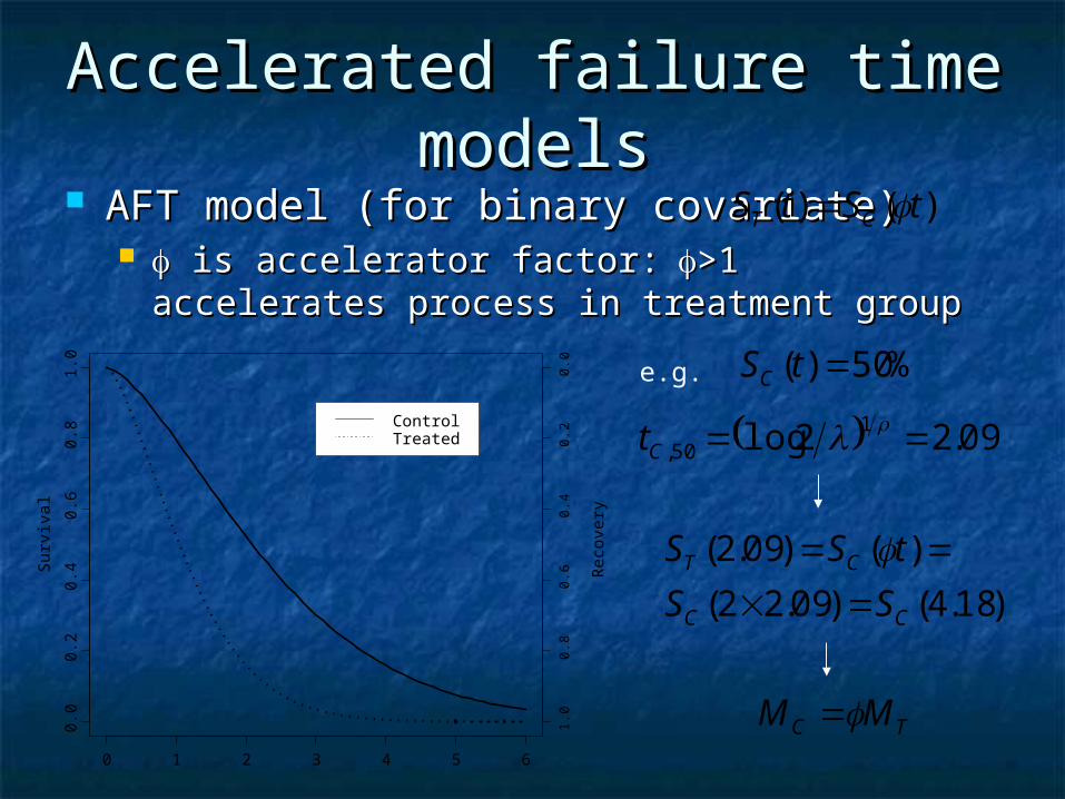
Accelerated failure time Accelerated failure time modelsmodels

AFT model (for binary covariate)AFT model (for binary covariate) is accelerator factor:is accelerator factor:>1 accelerates >1 accelerates

process in treatment groupprocess in treatment group

)()( tStS CT

Su

rviv

al

0 1 2 3 4 5 6

0.0

0.2

0.4

0.6

0.8

1.0

1.0

0.8

0.6

0.4

0.2

0.0

ControlTreated

Re

cove

ry

e.g.

09.22log 150, Ct

%50)( tSC

)18.4()09.22(

)()09.2(

CC

CT

SS

tSS

TC MM

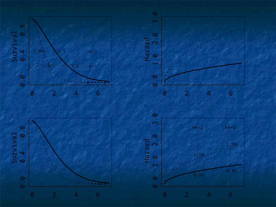
Proportional hazards (PH) Proportional hazards (PH) versus accelerated failure time versus accelerated failure time

(AFT)(AFT) PH model (for binary covariate)PH model (for binary covariate)

AFT model (for binary covariate)AFT model (for binary covariate)

)()( tStS CT

ijij xthth exp)()( 0 )()( 0 ththC

exp )()( 0 ththT )exp()(

)(

ratio Hazard

th

th

C

T

)()( 0 ththC

)()( 0 ththT ijijij xtxhth expexp)( 0

Su

rviv

al

0 2 4 6

0.0

0.4

0.8

1.05 2.1

1.6 3.2

Ha

zard

0 2 4 6

0.0

1.0

2.0

3.0

Su

rviv

al

0 2 4 6

0.0

0.4

0.8

Ha

zard

0 2 4 6

0.0

1.0

2.0

3.0

HR=2 HR=2

0.56

1.20

0.85

1.70

Log-linear model Log-linear model representationrepresentation

In most packages (SAS, R) survival models In most packages (SAS, R) survival models (and their estimates) are parametrized as (and their estimates) are parametrized as log linear modelslog linear models

If the error term If the error term eeijij has extreme value has extreme value distribution, then this model corresponds todistribution, then this model corresponds to PH Weibull model withPH Weibull model with

AFT Weibull model withAFT Weibull model with

ijijij exT log

)exp( 1

)exp( 1

Documents

Modeling clustered survival data The different approaches