Embed Size (px)
Citation preview
10 Dichotomous or binary responses
10.1 Introduction
Dichotomous or binary responses are widespread. Examples include being dead oralive, agreeing or disagreeing with a statement, and succeeding or failing to accomplishsomething. The responses are usually coded as 1 or 0, where 1 can be interpreted as theanswer “yes” and 0 as the answer “no” to some question. For instance, in section 10.2,we will consider the employment status of women where the question is whether thewomen are employed.
We start by briefly reviewing ordinary logistic and probit regression for dichotomousresponses, formulating the models both as generalized linear models, as is common instatistics and biostatistics, and as latent-response models, which is common in econo-metrics and psychometrics. This prepares the foundation for a discussion of variousapproaches for clustered dichotomous data, with special emphasis on random-interceptmodels. In this setting, the crucial distinction between conditional or subject-specificeffects and marginal or population-averaged effects is highlighted, and measures of de-pendence and heterogeneity are described.
We also discuss special features of statistical inference for random-intercept mod-els with clustered dichotomous responses, including maximum likelihood estimation ofmodel parameters, methods for assigning values to random effects, and how to obtaindifferent kinds of predicted probabilities. This more technical material is provided herebecause the principles apply to all models discussed in this volume. However, you canskip it (sections 10.11 through 10.13) on first reading because it is not essential forunderstanding and interpreting the models.
Other approaches to clustered data with binary responses, such as fixed-interceptmodels (conditional maximum likelihood) and generalized estimating equations (GEE)are briefly discussed in section 10.14.
10.2 Single-level logit and probit regression models for di-
chotomous responses
In this section, we will introduce logit and probit models without random effects thatare appropriate for datasets without any kind of clustering. For simplicity, we will startby considering just one covariate xi for unit (for example, subject) i. The models can
501
502 Chapter 10 Dichotomous or binary responses
be specified either as generalized linear models or as latent-response models. These twoapproaches and their relationship are described in sections 10.2.1 and 10.2.2.
10.2.1 Generalized linear model formulation
As in models for continuous responses, we are interested in the expectation (mean) ofthe response as a function of the covariate. The expectation of a binary (0 or 1) responseis just the probability that the response is 1:
E(yi|xi) = Pr(yi = 1|xi)
In linear regression, the conditional expectation of the response is modeled as a linearfunction E(yi|xi) = β1 + β2xi of the covariate (see section 1.5). For dichotomousresponses, this approach may be problematic because the probability must lie between0 and 1, whereas regression lines increase (or decrease) indefinitely as the covariateincreases (or decreases). Instead, a nonlinear function is specified in one of two ways:
Pr(yi = 1|xi) = h(β1 + β2xi)
org{Pr(yi = 1|xi)} = β1 + β2xi = νi
where νi (pronounced “nu”) is referred to as the linear predictor. These two formulationsare equivalent if the function h(·) is the inverse of the function g(·). Here g(·) is known asthe link function and h(·) as the inverse link function, sometimes written as g−1(·). Anappealing feature of generalized linear models is that they all involve a linear predictorresembling linear regression (without a residual error term). Therefore, we can handlecategorical explanatory variables, interactions, and flexible curved relationships by usingdummy variables, products of variables, and polynomials or splines, just as in linearregression.
Typical choices of link function for binary responses are the logit or probit links.In this section, we focus on the logit link, which is used for logistic regression, whereasboth links are discussed in section 10.2.2. For the logit link, the model can be writtenas
logit {Pr(yi = 1|xi)} ≡ ln
{Pr(yi = 1|xi)
1 − Pr(yi = 1|xi)
}
︸ ︷︷ ︸Odds(yi=1|xi)
= β1 + β2xi (10.1)
The fraction in parentheses in (10.1) represents the odds that yi =1 given xi, the ex-pected number of 1 responses per 0 response. The odds—or in other words, the expectednumber of successes per failure—is the standard way of representing the chances againstwinning in gambling. It follows from (10.1) that the logit model can alternatively beexpressed as an exponential function for the odds:
Odds(yi = 1|xi) = exp(β1 + β2xi)
10.2.1 Generalized linear model formulation 503
Because the relationship between odds and probabilities is
Odds =Pr
1 − Prand Pr =
Odds
1 + Odds
the probability that the response is 1 in the logit model is
Pr(yi = 1|xi) = logit−1(β1 + β2xi) ≡exp(β1 + β2xi)
1 + exp(β1 + β2xi)(10.2)
which is the inverse logit function (sometimes called logistic function) of the linearpredictor.
We have introduced two components of a generalized linear model: the linear predic-tor and the link function. The third component is the distribution of the response giventhe covariates. Letting πi ≡ Pr(yi = 1|xi), the distribution is specified as Bernoulli(πi),or equivalently as binomial(1, πi). There is no level-1 residual ǫi in (10.1), so the re-lationship between the probability and the covariate is deterministic. However, the re-sponses are random because the covariate determines only the probability. Whether theresponse is 0 or 1 is the result of a Bernoulli trial. A Bernoulli trial can be thought of astossing a biased coin with probability of heads equal to πi. It follows from the Bernoullidistribution that the relationship between the conditional variance of the response andits conditional mean πi, also known as the variance function, is Var(yi|xi) = πi(1− πi).(Including a residual ǫi in the linear predictor of binary regression models would leadto a model that is at best weakly identified1 unless the residual is shared between unitsin a cluster as in the multilevel models considered later in the chapter.)
The logit link is appealing because it produces a linear model for the log of the odds,implying a multiplicative model for the odds themselves. If we add one unit to xi, wemust add β2 to the log odds or multiply the odds by exp(β2). This can be seen byconsidering a 1-unit change in xi from some value a to a+1. The corresponding changein the log odds is
ln{Odds(yi = 1|xi = a+ 1)} − ln{Odds(yi = 1|xi = a)}= {β1 + β2(a+ 1)} − (β1 + β2a) = β2
Exponentiating both sides, we obtain the odds ratio (OR):
exp[ln{Odds(yi = 1|xi = a+ 1)} − ln{Odds(yi = 1|xi = a)}
]
=Odds(yi = 1|xi = a+ 1)
Odds(yi = 1|xi = a)=
Pr(yi = 1|xi = a+ 1)
Pr(yi = 0|xi = a+ 1)
/Pr(yi = 1|xi = a)
Pr(yi = 0|xi = a)
= exp(β2)
1. Formally, the model is identified by functional form. For instance, if xi is continuous, the level-1variance has a subtle effect on the shape of the relationship between Pr(yi = 1|xi) and xi. With aprobit link, single-level models with residuals are not identified.
504 Chapter 10 Dichotomous or binary responses
Consider now the case where several covariates—for instance, x2i and x3i—are in-cluded in the model:
logit {Pr(yi = 1|x2i, x3i)} = β1 + β2x2i + β3x3i
In this case, exp(β2) is interpreted as the odds ratio comparing x2i = a+1 with x2i = afor given x3i (controlling for x3i), and exp(β3) is the odds ratio comparing x3i = a+ 1with x3i = a for given x2i.
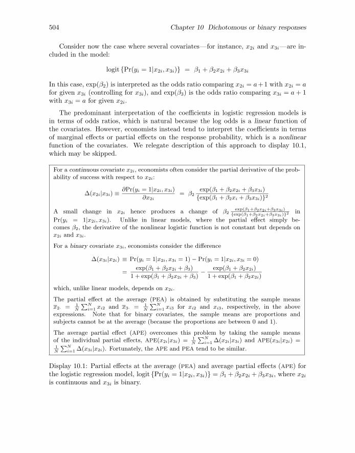
The predominant interpretation of the coefficients in logistic regression models isin terms of odds ratios, which is natural because the log odds is a linear function ofthe covariates. However, economists instead tend to interpret the coefficients in termsof marginal effects or partial effects on the response probability, which is a nonlinearfunction of the covariates. We relegate description of this approach to display 10.1,which may be skipped.
For a continuous covariate x2i, economists often consider the partial derivative of the prob-ability of success with respect to x2i:
∆(x2i|x3i) ≡∂Pr(yi = 1|x2i, x3i)
∂x2i= β2
exp(β1 + β2x2i + β3x3i)
{exp(β1 + β2xi + β3x3i)}2
A small change in x2i hence produces a change of β2exp(β1+β2x2i+β3x3i)
{exp(β1+β2x2i+β3x3i)}2 in
Pr(yi = 1|x2i, x3i). Unlike in linear models, where the partial effect simply be-comes β2, the derivative of the nonlinear logistic function is not constant but depends onx2i and x3i.
For a binary covariate x3i, economists consider the difference
∆(x3i|x2i) ≡ Pr(yi = 1|x2i, x3i = 1) − Pr(yi = 1|x2i, x3i = 0)
=exp(β1 + β2x2i + β3)
1 + exp(β1 + β2x2i + β3)− exp(β1 + β2x2i)
1 + exp(β1 + β2x2i)
which, unlike linear models, depends on x2i.
The partial effect at the average (PEA) is obtained by substituting the sample meansx2· = 1
N
PNi=1 xi2 and x3· = 1
N
PNi=1 xi3 for xi2 and xi3, respectively, in the above
expressions. Note that for binary covariates, the sample means are proportions andsubjects cannot be at the average (because the proportions are between 0 and 1).
The average partial effect (APE) overcomes this problem by taking the sample meansof the individual partial effects, APE(x2i|x3i) = 1
N
PNi=1 ∆(x2i|x3i) and APE(x3i|x2i) =
1N
PNi=1 ∆(x3i|x2i). Fortunately, the APE and PEA tend to be similar.
Display 10.1: Partial effects at the average (PEA) and average partial effects (APE) forthe logistic regression model, logit {Pr(yi = 1|x2i, x3i)} = β1 + β2x2i + β3x3i, where x2i
is continuous and x3i is binary.

10.2.1 Generalized linear model formulation 505
To illustrate logistic regression, we will consider data on married women from theCanadian Women’s Labor Force Participation Dataset used by Fox (1997). The datasetwomenlf.dta contains women’s employment status and two explanatory variables:
• workstat: employment status(0: not working; 1: employed part time; 2: employed full time)
• husbinc: husband’s income in $1,000
• chilpres: child present in household (dummy variable)
The dataset can be retrieved by typing
. use http://www.stata-press.com/data/mlmus3/womenlf
Fox (1997) considered a multiple logistic regression model for a woman being em-ployed (full or part time) versus not working with covariates husbinc and chilpres
logit{Pr(yi =1|xi)} = β1 + β2x2i + β3x3i
where yi = 1 denotes employment, yi = 0 denotes not working, x2i is husbinc, x3i ischilpres, and xi = (x2i, x3i)
′ is a vector containing both covariates.
We first merge categories 1 and 2 (employed part time and full time) of workstat
into a new category 1 for being employed,
. recode workstat 2=1
and then fit the model by maximum likelihood using Stata’s logit command:
. logit workstat husbinc chilpres
Logistic regression Number of obs = 263LR chi2(2) = 36.42Prob > chi2 = 0.0000
Log likelihood = -159.86627 Pseudo R2 = 0.1023
workstat Coef. Std. Err. z P>|z| [95% Conf. Interval]
husbinc -.0423084 .0197801 -2.14 0.032 -.0810768 -.0035401chilpres -1.575648 .2922629 -5.39 0.000 -2.148473 -1.002824
_cons 1.33583 .3837632 3.48 0.000 .5836674 2.087992
The estimated coefficients are negative, so the estimated log odds of employment arelower if the husband earns more and if there is a child in the household. At the 5%significance level, we can reject the null hypotheses that the individual coefficients β2
and β3 are zero. The estimated coefficients and their estimated standard errors are alsogiven in table 10.1.
506 Chapter 10 Dichotomous or binary responses
Table 10.1: Maximum likelihood estimates for logistic regression model for women’slabor force participation
Est (SE) OR=exp(β) (95% CI)β1 [ cons] 1.34 (0.38)β2 [husbinc] −0.04 (0.02) 0.96 (0.92, 1.00)β3 [chilpres] −1.58 (0.29) 0.21 (0.12, 0.37)
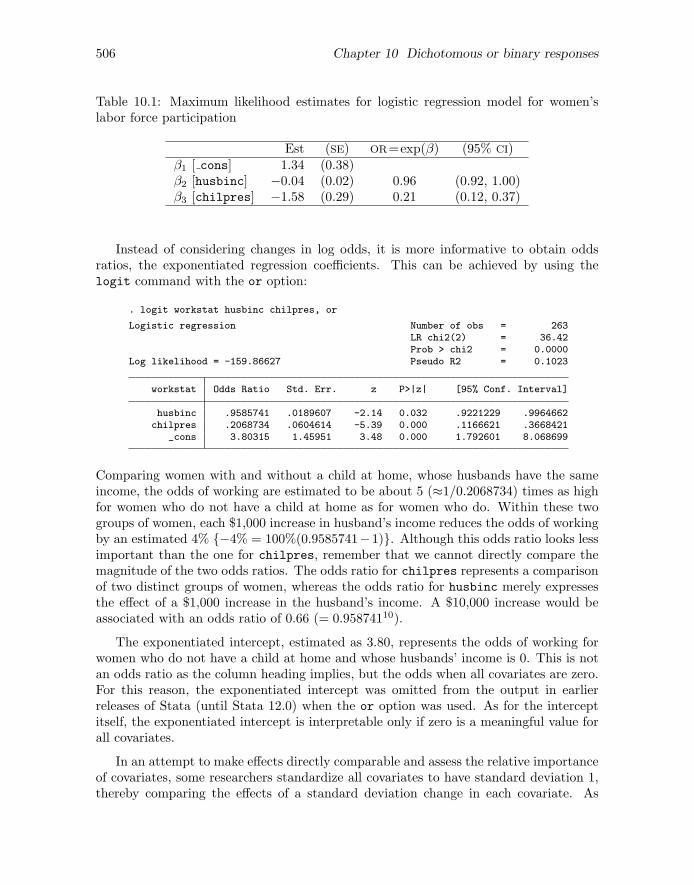
Instead of considering changes in log odds, it is more informative to obtain oddsratios, the exponentiated regression coefficients. This can be achieved by using thelogit command with the or option:
. logit workstat husbinc chilpres, or
Logistic regression Number of obs = 263LR chi2(2) = 36.42Prob > chi2 = 0.0000
Log likelihood = -159.86627 Pseudo R2 = 0.1023
workstat Odds Ratio Std. Err. z P>|z| [95% Conf. Interval]
husbinc .9585741 .0189607 -2.14 0.032 .9221229 .9964662chilpres .2068734 .0604614 -5.39 0.000 .1166621 .3668421
_cons 3.80315 1.45951 3.48 0.000 1.792601 8.068699
Comparing women with and without a child at home, whose husbands have the sameincome, the odds of working are estimated to be about 5 (≈1/0.2068734) times as highfor women who do not have a child at home as for women who do. Within these twogroups of women, each $1,000 increase in husband’s income reduces the odds of workingby an estimated 4% {−4% = 100%(0.9585741−1)}. Although this odds ratio looks lessimportant than the one for chilpres, remember that we cannot directly compare themagnitude of the two odds ratios. The odds ratio for chilpres represents a comparisonof two distinct groups of women, whereas the odds ratio for husbinc merely expressesthe effect of a $1,000 increase in the husband’s income. A $10,000 increase would beassociated with an odds ratio of 0.66 (= 0.95874110).
The exponentiated intercept, estimated as 3.80, represents the odds of working forwomen who do not have a child at home and whose husbands’ income is 0. This is notan odds ratio as the column heading implies, but the odds when all covariates are zero.For this reason, the exponentiated intercept was omitted from the output in earlierreleases of Stata (until Stata 12.0) when the or option was used. As for the interceptitself, the exponentiated intercept is interpretable only if zero is a meaningful value forall covariates.
In an attempt to make effects directly comparable and assess the relative importanceof covariates, some researchers standardize all covariates to have standard deviation 1,thereby comparing the effects of a standard deviation change in each covariate. As

10.2.1 Generalized linear model formulation 507
discussed in section 1.5, there are many problems with such an approach, one of thembeing the meaningless notion of a standard deviation change in a dummy variable, suchas chilpres.
The standard errors of exponentiated estimated regression coefficients should gener-ally not be used for confidence intervals or hypothesis tests. Instead, the 95% confidenceintervals in the above output were computed by taking the exponentials of the confidencelimits for the regression coefficients β:
exp{β ± 1.96×SE(β)}
In table 10.1, we therefore report estimated odds ratios with 95% confidence intervalsinstead of standard errors.
To visualize the model, we can produce a plot of the predicted probabilities versushusbinc, with separate curves for women with and without children at home. Pluggingin maximum likelihood estimates for the parameters in (10.2), the predicted probabilityfor woman i, often denoted πi, is given by the inverse logit of the estimated linearpredictor
πi ≡ Pr(yi = 1|xi) =exp(β1 + β2x2i + β3x3i)
1 + exp(β1 + β2x2i + β3x3i)= logit−1(β1 + β2x2i + β3x3i)
(10.3)and can be obtained for the women in the dataset by using the predict command withthe pr option:
. predict prob, pr
We can now produce the graph of predicted probabilities, shown in figure 10.1, by using
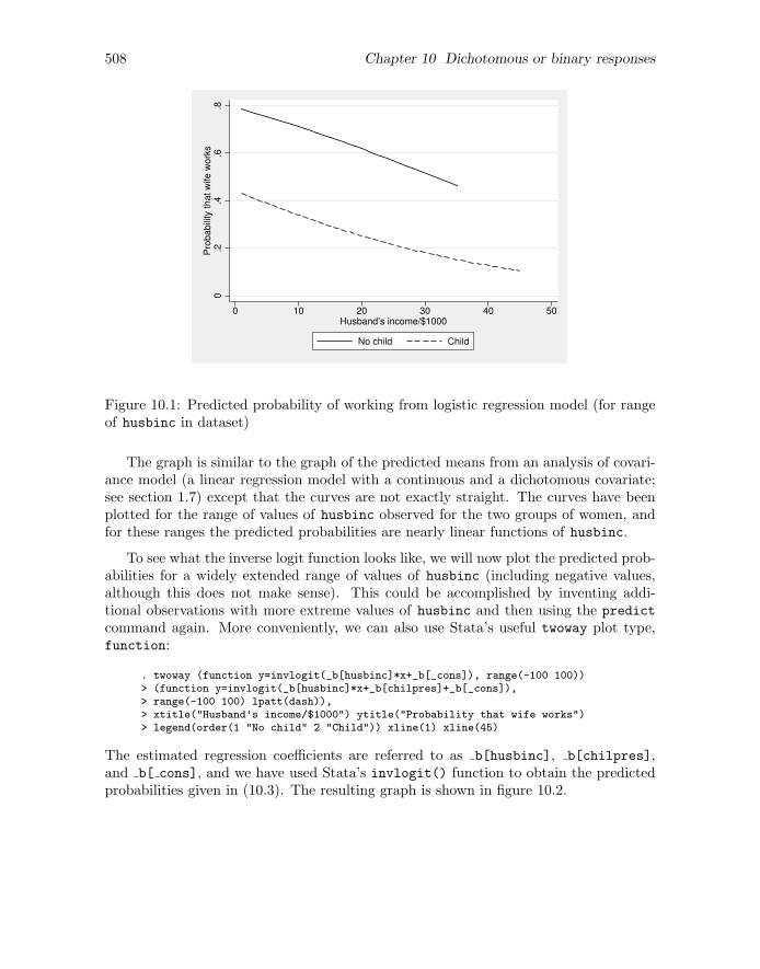
. twoway (line prob husbinc if chilpres==0, sort)> (line prob husbinc if chilpres==1, sort lpatt(dash)),> legend(order(1 "No child" 2 "Child"))> xtitle("Husband’s income/$1000") ytitle("Probability that wife works")
508 Chapter 10 Dichotomous or binary responses
0.2
.4.6
.8P
robabili
ty that w
ife w
ork
s
0 10 20 30 40 50Husband’s income/$1000
No child Child
Figure 10.1: Predicted probability of working from logistic regression model (for rangeof husbinc in dataset)
The graph is similar to the graph of the predicted means from an analysis of covari-ance model (a linear regression model with a continuous and a dichotomous covariate;see section 1.7) except that the curves are not exactly straight. The curves have beenplotted for the range of values of husbinc observed for the two groups of women, andfor these ranges the predicted probabilities are nearly linear functions of husbinc.
To see what the inverse logit function looks like, we will now plot the predicted prob-abilities for a widely extended range of values of husbinc (including negative values,although this does not make sense). This could be accomplished by inventing addi-tional observations with more extreme values of husbinc and then using the predict
command again. More conveniently, we can also use Stata’s useful twoway plot type,function:
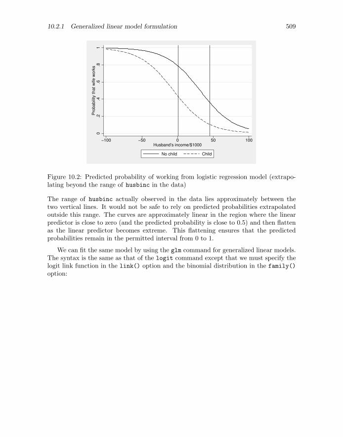
. twoway (function y=invlogit(_b[husbinc]*x+_b[_cons]), range(-100 100))> (function y=invlogit(_b[husbinc]*x+_b[chilpres]+_b[_cons]),> range(-100 100) lpatt(dash)),> xtitle("Husband’s income/$1000") ytitle("Probability that wife works")> legend(order(1 "No child" 2 "Child")) xline(1) xline(45)
The estimated regression coefficients are referred to as b[husbinc], b[chilpres],and b[ cons], and we have used Stata’s invlogit() function to obtain the predictedprobabilities given in (10.3). The resulting graph is shown in figure 10.2.
10.2.1 Generalized linear model formulation 509
0.2
.4.6
.81
Pro
babili
ty that w
ife w
ork
s
−100 −50 0 50 100Husband’s income/$1000
No child Child
Figure 10.2: Predicted probability of working from logistic regression model (extrapo-lating beyond the range of husbinc in the data)
The range of husbinc actually observed in the data lies approximately between thetwo vertical lines. It would not be safe to rely on predicted probabilities extrapolatedoutside this range. The curves are approximately linear in the region where the linearpredictor is close to zero (and the predicted probability is close to 0.5) and then flattenas the linear predictor becomes extreme. This flattening ensures that the predictedprobabilities remain in the permitted interval from 0 to 1.
We can fit the same model by using the glm command for generalized linear models.The syntax is the same as that of the logit command except that we must specify thelogit link function in the link() option and the binomial distribution in the family()
option:
510 Chapter 10 Dichotomous or binary responses
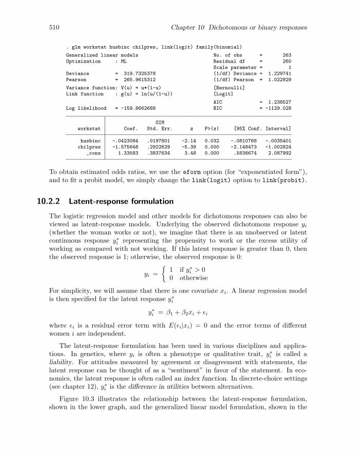
. glm workstat husbinc chilpres, link(logit) family(binomial)
Generalized linear models No. of obs = 263Optimization : ML Residual df = 260
Scale parameter = 1Deviance = 319.7325378 (1/df) Deviance = 1.229741Pearson = 265.9615312 (1/df) Pearson = 1.022929
Variance function: V(u) = u*(1-u) [Bernoulli]Link function : g(u) = ln(u/(1-u)) [Logit]
AIC = 1.238527Log likelihood = -159.8662689 BIC = -1129.028
OIMworkstat Coef. Std. Err. z P>|z| [95% Conf. Interval]
husbinc -.0423084 .0197801 -2.14 0.032 -.0810768 -.0035401chilpres -1.575648 .2922629 -5.39 0.000 -2.148473 -1.002824
_cons 1.33583 .3837634 3.48 0.000 .5836674 2.087992
To obtain estimated odds ratios, we use the eform option (for “exponentiated form”),and to fit a probit model, we simply change the link(logit) option to link(probit).
10.2.2 Latent-response formulation
The logistic regression model and other models for dichotomous responses can also beviewed as latent-response models. Underlying the observed dichotomous response yi
(whether the woman works or not), we imagine that there is an unobserved or latentcontinuous response y∗i representing the propensity to work or the excess utility ofworking as compared with not working. If this latent response is greater than 0, thenthe observed response is 1; otherwise, the observed response is 0:
yi =
{1 if y∗i > 00 otherwise
For simplicity, we will assume that there is one covariate xi. A linear regression modelis then specified for the latent response y∗i
y∗i = β1 + β2xi + ǫi
where ǫi is a residual error term with E(ǫi|xi) = 0 and the error terms of differentwomen i are independent.
The latent-response formulation has been used in various disciplines and applica-tions. In genetics, where yi is often a phenotype or qualitative trait, y∗i is called aliability. For attitudes measured by agreement or disagreement with statements, thelatent response can be thought of as a “sentiment” in favor of the statement. In eco-nomics, the latent response is often called an index function. In discrete-choice settings(see chapter 12), y∗i is the difference in utilities between alternatives.
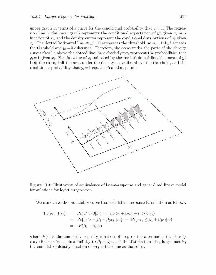
Figure 10.3 illustrates the relationship between the latent-response formulation,shown in the lower graph, and the generalized linear model formulation, shown in the
10.2.2 Latent-response formulation 511
upper graph in terms of a curve for the conditional probability that yi =1. The regres-sion line in the lower graph represents the conditional expectation of y∗i given xi as afunction of xi, and the density curves represent the conditional distributions of y∗i givenxi. The dotted horizontal line at y∗i =0 represents the threshold, so yi =1 if y∗i exceedsthe threshold and yi =0 otherwise. Therefore, the areas under the parts of the densitycurves that lie above the dotted line, here shaded gray, represent the probabilities thatyi =1 given xi. For the value of xi indicated by the vertical dotted line, the mean of y∗iis 0; therefore, half the area under the density curve lies above the threshold, and theconditional probability that yi =1 equals 0.5 at that point.
Pr(yi
=1|x
i)
0.5
0.0
xi
y∗i
Figure 10.3: Illustration of equivalence of latent-response and generalized linear modelformulations for logistic regression
We can derive the probability curve from the latent-response formulation as follows:
Pr(yi =1|xi) = Pr(y∗i > 0|xi) = Pr(β1 + β2xi + ǫi > 0|xi)
= Pr{ǫi > −(β1 + β2xi)|xi} = Pr(−ǫi ≤ β1 + β2xi|xi)
= F (β1 + β2xi)
where F (·) is the cumulative density function of −ǫi, or the area under the densitycurve for −ǫi from minus infinity to β1 + β2xi. If the distribution of ǫi is symmetric,the cumulative density function of −ǫi is the same as that of ǫi.
512 Chapter 10 Dichotomous or binary responses
Logistic regression
In logistic regression, ǫi is assumed to have a standard logistic cumulative density func-tion given xi,
Pr(ǫi < τ |xi) =exp(τ)
1 + exp(τ)
For this distribution, ǫi has mean zero and variance π2/3 ≈ 3.29 (note that π hererepresents the famous mathematical constant pronounced “pi”, the circumference of acircle divided by its diameter).
Probit regression
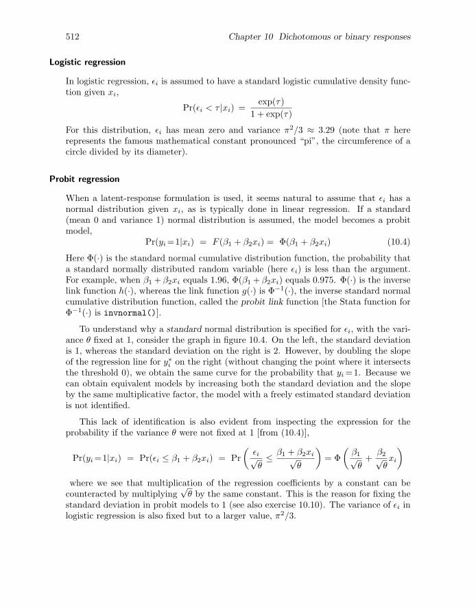
When a latent-response formulation is used, it seems natural to assume that ǫi has anormal distribution given xi, as is typically done in linear regression. If a standard(mean 0 and variance 1) normal distribution is assumed, the model becomes a probitmodel,
Pr(yi =1|xi) = F (β1 + β2xi) = Φ(β1 + β2xi) (10.4)
Here Φ(·) is the standard normal cumulative distribution function, the probability thata standard normally distributed random variable (here ǫi) is less than the argument.For example, when β1 + β2xi equals 1.96, Φ(β1 + β2xi) equals 0.975. Φ(·) is the inverselink function h(·), whereas the link function g(·) is Φ−1(·), the inverse standard normalcumulative distribution function, called the probit link function [the Stata function forΦ−1(·) is invnormal()].
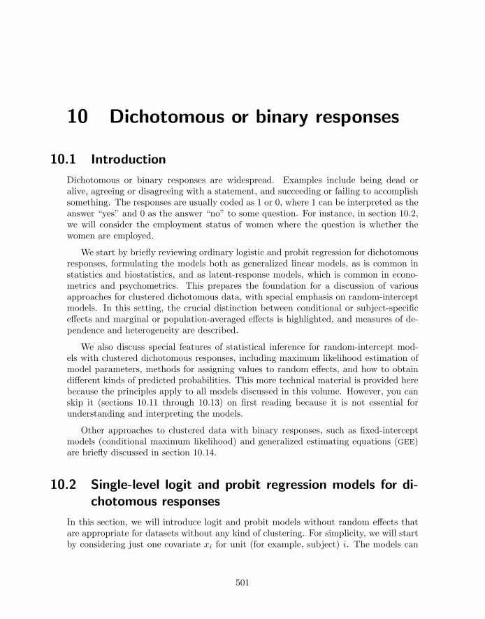
To understand why a standard normal distribution is specified for ǫi, with the vari-ance θ fixed at 1, consider the graph in figure 10.4. On the left, the standard deviationis 1, whereas the standard deviation on the right is 2. However, by doubling the slopeof the regression line for y∗i on the right (without changing the point where it intersectsthe threshold 0), we obtain the same curve for the probability that yi =1. Because wecan obtain equivalent models by increasing both the standard deviation and the slopeby the same multiplicative factor, the model with a freely estimated standard deviationis not identified.
This lack of identification is also evident from inspecting the expression for theprobability if the variance θ were not fixed at 1 [from (10.4)],
Pr(yi =1|xi) = Pr(ǫi ≤ β1 + β2xi) = Pr
(ǫi√θ≤ β1 + β2xi√
θ
)= Φ
(β1√θ
+β2√θxi
)
where we see that multiplication of the regression coefficients by a constant can becounteracted by multiplying
√θ by the same constant. This is the reason for fixing the
standard deviation in probit models to 1 (see also exercise 10.10). The variance of ǫi inlogistic regression is also fixed but to a larger value, π2/3.

10.2.2 Latent-response formulation 513
Pr(yi
=1|x
i)
0.0 xi
xi
y∗i
Figure 10.4: Illustration of equivalence between probit models with change in residualstandard deviation counteracted by change in slope
A probit model can be fit to the women’s employment data in Stata by using theprobit command:
. probit workstat husbinc chilpres
Probit regression Number of obs = 263LR chi2(2) = 36.19Prob > chi2 = 0.0000
Log likelihood = -159.97986 Pseudo R2 = 0.1016
workstat Coef. Std. Err. z P>|z| [95% Conf. Interval]
husbinc -.0242081 .0114252 -2.12 0.034 -.0466011 -.001815chilpres -.9706164 .1769051 -5.49 0.000 -1.317344 -.6238887
_cons .7981507 .2240082 3.56 0.000 .3591028 1.237199
These estimates are closer to zero than those reported for the logit model in table 10.1because the standard deviation of ǫi is 1 for the probit model and π/
√3 ≈ 1.81 for the
logit model. Therefore, as we have already seen in figure 10.4, the regression coefficientsin logit models must be larger in absolute value to produce nearly the same curve forthe conditional probability that yi = 1. Here we say “nearly the same” because theshapes of the probit and logit curves are similar yet not identical. To visualize the
514 Chapter 10 Dichotomous or binary responses
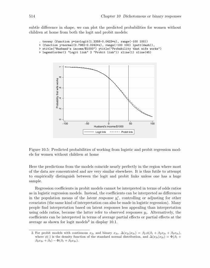
subtle difference in shape, we can plot the predicted probabilities for women withoutchildren at home from both the logit and probit models:
. twoway (function y=invlogit(1.3358-0.0423*x), range(-100 100))> (function y=normal(0.7982-0.0242*x), range(-100 100) lpatt(dash)),> xtitle("Husband’s income/$1000") ytitle("Probability that wife works")> legend(order(1 "Logit link" 2 "Probit link")) xline(1) xline(45)
0.2
.4.6
.81
Pro
babili
ty that w
ife w
ork
s
−100 −50 0 50 100Husband’s income/$1000
Logit link Probit link
Figure 10.5: Predicted probabilities of working from logistic and probit regression mod-els for women without children at home
Here the predictions from the models coincide nearly perfectly in the region where mostof the data are concentrated and are very similar elsewhere. It is thus futile to attemptto empirically distinguish between the logit and probit links unless one has a hugesample.
Regression coefficients in probit models cannot be interpreted in terms of odds ratiosas in logistic regression models. Instead, the coefficients can be interpreted as differencesin the population means of the latent response y∗i , controlling or adjusting for othercovariates (the same kind of interpretation can also be made in logistic regression). Manypeople find interpretation based on latent responses less appealing than interpretationusing odds ratios, because the latter refer to observed responses yi. Alternatively, thecoefficients can be interpreted in terms of average partial effects or partial effects at theaverage as shown for logit models2 in display 10.1.
2. For probit models with continuous x2i and binary x3i, ∆(x2i|x3i) = β2 φ(β1 + β2x2i + β3x3i),where φ(·) is the density function of the standard normal distribution, and ∆(x3i|x2i) = Φ(β1 +β2x2i + β3) − Φ(β1 + β2x2i).

10.4 Longitudinal data structure 515
10.3 Which treatment is best for toenail infection?
Lesaffre and Spiessens (2001) analyzed data provided by De Backer et al. (1998) froma randomized, double-blind trial of treatments for toenail infection (dermatophyte ony-chomycosis). Toenail infection is common, with a prevalence of about 2% to 3% inthe United States and a much higher prevalence among diabetics and the elderly. Theinfection is caused by a fungus, and not only disfigures the nails but also can causephysical pain and impair the ability to work.
In this clinical trial, 378 patients were randomly allocated into two oral antifungaltreatments (250 mg/day terbinafine and 200 mg/day itraconazole) and evaluated atseven visits, at weeks 0, 4, 8, 12, 24, 36, and 48. One outcome is onycholysis, the degreeof separation of the nail plate from the nail bed, which was dichotomized (“moderateor severe” versus “none or mild”) and is available for 294 patients.
The dataset toenail.dta contains the following variables:
• patient: patient identifier
• outcome: onycholysis (separation of nail plate from nail bed)(0: none or mild; 1: moderate or severe)
• treatment: treatment group (0: itraconazole; 1: terbinafine)
• visit: visit number (1, 2, . . . , 7)
• month: exact timing of visit in months
We read in the toenail data by typing
. use http://www.stata-press.com/data/mlmus3/toenail, clear
The main research question is whether the treatments differ in their efficacy. Inother words, do patients receiving one treatment experience a greater decrease in theirprobability of having onycholysis than those receiving the other treatment?
10.4 Longitudinal data structure
Before investigating the research question, we should look at the longitudinal structureof the toenail data using, for instance, the xtdescribe, xtsum, and xttab commands,discussed in Introduction to models for longitudinal and panel data (part III).
Here we illustrate the use of the xtdescribe command, which can be used for thesedata because the data were intended to be balanced with seven visits planned for thesame set of weeks for each patient (although the exact timing of the visits varied betweenpatients).
516 Chapter 10 Dichotomous or binary responses
Before using xtdescribe, we xtset the data with patient as the cluster identifierand visit as the time variable:
. xtset patient visitpanel variable: patient (unbalanced)time variable: visit, 1 to 7, but with gaps
delta: 1 unit
The output states that the data are unbalanced and that there are gaps. [We woulddescribe the time variable visit as balanced because the values are identical acrosspatients apart from the gaps caused by missing data; see the introduction to models forlongitudinal and panel data (part III in volume I).]
To explore the missing-data patterns, we use
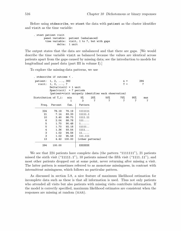
. xtdescribe if outcome < .
patient: 1, 2, ..., 383 n = 294visit: 1, 2, ..., 7 T = 7
Delta(visit) = 1 unitSpan(visit) = 7 periods(patient*visit uniquely identifies each observation)
Distribution of T_i: min 5% 25% 50% 75% 95% max1 3 7 7 7 7 7
Freq. Percent Cum. Pattern
224 76.19 76.19 111111121 7.14 83.33 11111.110 3.40 86.73 1111.116 2.04 88.78 111....5 1.70 90.48 1......5 1.70 92.18 11111..4 1.36 93.54 1111...3 1.02 94.56 11.....3 1.02 95.58 111.11113 4.42 100.00 (other patterns)
294 100.00 XXXXXXX
We see that 224 patients have complete data (the pattern “1111111”), 21 patientsmissed the sixth visit (“11111.1”), 10 patients missed the fifth visit (“1111.11”), andmost other patients dropped out at some point, never returning after missing a visit.The latter pattern is sometimes referred to as monotone missingness, in contrast withintermittent missingness, which follows no particular pattern.
As discussed in section 5.8, a nice feature of maximum likelihood estimation forincomplete data such as these is that all information is used. Thus not only patientswho attended all visits but also patients with missing visits contribute information. Ifthe model is correctly specified, maximum likelihood estimates are consistent when theresponses are missing at random (MAR).

10.5 Proportions and fitted population-averaged or marginal probabilities 517
10.5 Proportions and fitted population-averaged or
marginal probabilities
A useful graphical display of the data is a bar plot showing the proportion of patientswith onycholysis at each visit by treatment group. The following Stata commands canbe used to produce the graph shown in figure 10.6:
. label define tr 0 "Itraconazole" 1 "Terbinafine"
. label values treatment tr
. graph bar (mean) proportion = outcome, over(visit) by(treatment)> ytitle(Proportion with onycholysis)
Here we defined value labels for treatment to make them appear on the graph.
0.1
.2.3
.4
1 2 3 4 5 6 7 1 2 3 4 5 6 7
Itraconazole Terbinafine
Pro
port
ion w
ith o
nycholy
sis
Graphs by treatment
Figure 10.6: Bar plot of proportion of patients with toenail infection by visit and treat-ment group
We used the visit number visit to define the bars instead of the exact timing of thevisit month because there would generally not be enough patients with the same timingto estimate the proportions reliably. An alternative display is a line graph, plotting theobserved proportions at each visit against time. For this graph, it is better to use theaverage time associated with each visit for the x axis than to use visit number, becausethe visits were not equally spaced. Both the proportions and the average times for eachvisit in each treatment group can be obtained using the egen command with the mean()function:
518 Chapter 10 Dichotomous or binary responses
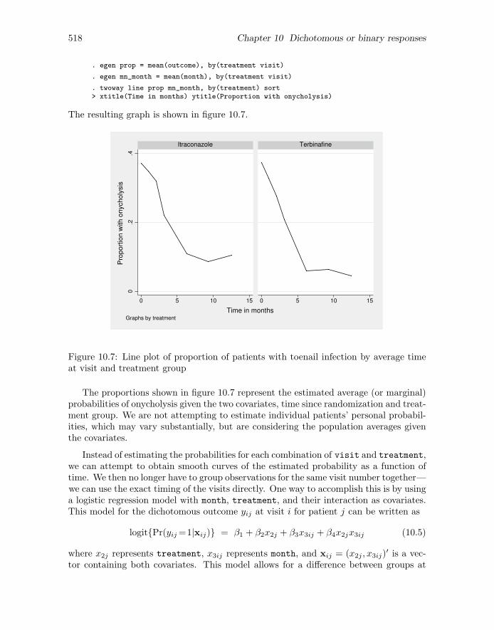
. egen prop = mean(outcome), by(treatment visit)
. egen mn_month = mean(month), by(treatment visit)
. twoway line prop mn_month, by(treatment) sort> xtitle(Time in months) ytitle(Proportion with onycholysis)
The resulting graph is shown in figure 10.7.
0.2
.4
0 5 10 15 0 5 10 15
Itraconazole Terbinafine
Pro
port
ion w
ith o
nycholy
sis
Time in monthsGraphs by treatment
Figure 10.7: Line plot of proportion of patients with toenail infection by average timeat visit and treatment group
The proportions shown in figure 10.7 represent the estimated average (or marginal)probabilities of onycholysis given the two covariates, time since randomization and treat-ment group. We are not attempting to estimate individual patients’ personal probabil-ities, which may vary substantially, but are considering the population averages giventhe covariates.
Instead of estimating the probabilities for each combination of visit and treatment,we can attempt to obtain smooth curves of the estimated probability as a function oftime. We then no longer have to group observations for the same visit number together—we can use the exact timing of the visits directly. One way to accomplish this is by usinga logistic regression model with month, treatment, and their interaction as covariates.This model for the dichotomous outcome yij at visit i for patient j can be written as
logit{Pr(yij =1|xij)} = β1 + β2x2j + β3x3ij + β4x2jx3ij (10.5)
where x2j represents treatment, x3ij represents month, and xij = (x2j , x3ij)′ is a vec-
tor containing both covariates. This model allows for a difference between groups at
10.5 Proportions and fitted population-averaged or marginal probabilities 519
baseline β2, and linear changes in the log odds of onycholysis over time with slope β3
in the itraconazole group and slope β3 + β4 in the terbinafine group. Therefore, β4, thedifference in the rate of improvement (on the log odds scale) between treatment groups,can be viewed as the treatment effect (terbinafine versus itraconazole).
This model makes the unrealistic assumption that the responses for a given patientare conditionally independent after controlling for the included covariates. We will relaxthis assumption in the next section. Here we can get satisfactory inferences for marginaleffects by using robust standard errors for clustered data instead of using model-basedstandard errors. This approach is analogous to pooled OLS in linear models and corre-sponds to the generalized estimating equations approach discussed in section 6.6 with anindependence working correlation structure (see 10.14.2 for an example with a differentworking correlation matrix).
We start by constructing an interaction term, trt month, for treatment and month,
. generate trt_month = treatment*month
before fitting the model by maximum likelihood with robust standard errors:
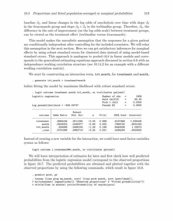
. logit outcome treatment month trt_month, or vce(cluster patient)
Logistic regression Number of obs = 1908Wald chi2(3) = 64.30Prob > chi2 = 0.0000
Log pseudolikelihood = -908.00747 Pseudo R2 = 0.0830
Robustoutcome Odds Ratio Std. Err. z P>|z| [95% Conf. Interval]
treatment .9994184 .2511294 -0.00 0.998 .6107468 1.635436month .8434052 .0246377 -5.83 0.000 .7964725 .8931034
trt_month .934988 .0488105 -1.29 0.198 .8440528 1.03572_cons .5731389 .0982719 -3.25 0.001 .4095534 .8020642
Instead of creating a new variable for the interaction, we could have used factor-variablessyntax as follows:
logit outcome i.treatment##c.month, or vce(cluster patient)
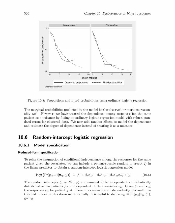
We will leave interpretation of estimates for later and first check how well predictedprobabilities from the logistic regression model correspond to the observed proportionsin figure 10.7. The predicted probabilities are obtained and plotted together with theobserved proportions by using the following commands, which result in figure 10.8.
. predict prob, pr
. twoway (line prop mn_month, sort) (line prob month, sort lpatt(dash)),> by(treatment) legend(order(1 "Observed proportions" 2 "Fitted probabilities"))> xtitle(Time in months) ytitle(Probability of onycholysis)
520 Chapter 10 Dichotomous or binary responses
0.2
.4
0 5 10 15 20 0 5 10 15 20
Itraconazole Terbinafine
Observed proportions Fitted probabilities
Pro
babili
ty o
f onycholy
sis
Time in months
Graphs by treatment
Figure 10.8: Proportions and fitted probabilities using ordinary logistic regression
The marginal probabilities predicted by the model fit the observed proportions reason-ably well. However, we have treated the dependence among responses for the samepatient as a nuisance by fitting an ordinary logistic regression model with robust stan-dard errors for clustered data. We now add random effects to model the dependenceand estimate the degree of dependence instead of treating it as a nuisance.
10.6 Random-intercept logistic regression
10.6.1 Model specification
Reduced-form specification
To relax the assumption of conditional independence among the responses for the samepatient given the covariates, we can include a patient-specific random intercept ζj inthe linear predictor to obtain a random-intercept logistic regression model
logit{Pr(yij =1|xij , ζj)} = β1 + β2x2j + β3x3ij + β4x2jx3ij + ζj (10.6)
The random intercepts ζj ∼ N(0, ψ) are assumed to be independent and identicallydistributed across patients j and independent of the covariates xij . Given ζj and xij ,the responses yij for patient j at different occasions i are independently Bernoulli dis-tributed. To write this down more formally, it is useful to define πij ≡ Pr(yij |xij , ζj),giving
10.6.1 Model specification 521
logit(πij) = β1 + β2x2j + β3x3ij + β4x2jx3ij + ζj
yij |πij ∼ Binomial(1, πij)
This is a simple example of a generalized linear mixed model (GLMM) because it isa generalized linear model with both fixed effects β1 to β4 and a random effect ζj . Themodel is also sometimes referred to as a hierarchical generalized linear model (HGLM)in contrast to a hierarchical linear model (HLM). The random intercept can be thoughtof as the combined effect of omitted patient-specific (time-constant) covariates thatcause some patients to be more prone to onycholysis than others (more precisely, thecomponent of this combined effect that is independent of the covariates in the model—not an issue if the covariates are exogenous). It is appealing to model this unobservedheterogeneity in the same way as observed heterogeneity by simply adding the randomintercept to the linear predictor. As we will explain later, be aware that odds ratiosobtained by exponentiating regression coefficients in this model must be interpretedconditionally on the random intercept and are therefore often referred to as conditionalor subject-specific odds ratios.
Using the latent-response formulation, the model can equivalently be written as
y∗ij = β1 + β2x2j + β3x3ij + β4x2jx3ij + ζj + ǫij (10.7)
where ζj ∼ N(0, ψ) and the ǫij have standard logistic distributions. The binary re-sponses yij are determined by the latent continuous responses via the threshold model
yij =
{1 if y∗ij > 0
0 otherwise
Confusingly, logistic random-effects models are sometimes written as yij = πij + eij ,where eij is a normally distributed level-1 residual with variance πij(1 − πij). Thisformulation is clearly incorrect because such a model does not produce binary responses(see Skrondal and Rabe-Hesketh [2007]).
In both formulations of the model (via a logit link or in terms of a latent response), itis assumed that the ζj are independent across patients and independent of the covariatesxij at occasion i. It is also assumed that the covariates at other occasions do notaffect the response probabilities given the random intercept (called strict exogeneityconditional on the random intercept). For the latent response formulation, the ǫij areassumed to be independent across both occasions and patients, and independent of bothζj and xij . In the generalized linear model formulation, the analogous assumptions areimplicit in assuming that the responses are independently Bernoulli distributed (withprobabilities determined by ζj and xij).
In contrast to linear random effects models, consistent estimation in random-effectslogistic regression requires that the random part of the model is correctly specified in
522 Chapter 10 Dichotomous or binary responses
addition to the fixed part. Specifically, consistency formally requires (1) a correct linearpredictor (such as including relevant interactions), (2) a correct link function, (3) cor-rect specification of covariates having random coefficients, (4) conditional independenceof responses given the random effects and covariates, (5) independence of the randomeffects and covariates (for causal inference), and (6) normally distributed random ef-fects. Hence, the assumptions are stronger than those discussed for linear models insection 3.3.2. However, the normality assumption for the random intercepts seems tobe rather innocuous in contrast to the assumption of independence between the ran-dom intercepts and covariates (Heagerty and Kurland 2001). As in standard logisticregression, the ML estimator is not necessarily unbiased in finite samples even if all theassumptions are true.
Two-stage formulation
Raudenbush and Bryk (2002) and others write two-level models in terms of a level-1model and one or more level-2 models (see section 4.9). In generalized linear mixedmodels, the need to specify a link function and distribution leads to two further stagesof model specification.
Using the notation and terminology of Raudenbush and Bryk (2002), the level-1sampling model, link function, and structural model are written as
yij ∼ Bernoulli(ϕij)
logit(ϕij) = ηij
ηij = β0j + β1jx2j + β2jx3ij + β3jx2jx3ij
respectively.
The level-2 model for the intercept β0j is written as
β0j = γ00 + u0j
where γ00 is a fixed intercept and u0j is a residual or random intercept. The level-2models for the coefficients β1j , β2j , and β3j have no residuals for a random-interceptmodel,
βpj = γp0, p = 1, 2, 3
Plugging the level-2 models into the level-1 structural model, we obtain
ηij = γ00 + u0j + γ01x2j + γ02x3ij + γ03x2jx3ij
≡ β1 + ζ0j + β2x2j + β3x3ij + β4x2jx3ij
Equivalent models can be specified using either the reduced-form formulation (usedfor instance by Stata) or the two-stage formulation (used in the HLM software ofRaudenbush et al. 2004). However, in practice, model specification is to some extentinfluenced by the approach adopted as discussed in section 4.9.

10.7.1 Using xtlogit 523
10.7 Estimation of random-intercept logistic models
As of Stata 10, there are three commands for fitting random-intercept logistic models inStata: xtlogit, xtmelogit, and gllamm. All three commands provide maximum likeli-hood estimation and use adaptive quadrature to approximate the integrals involved (seesection 10.11.1 for more information). The commands have essentially the same syn-tax as their counterparts for linear models discussed in volume I. Specifically, xtlogitcorresponds to xtreg, xtmelogit corresponds to xtmixed, and gllamm uses essentiallythe same syntax for linear, logistic, and other types of models.
All three commands are relatively slow because they use numerical integration, butfor random-intercept models, xtlogit is much faster than xtmelogit, which is usu-ally faster than gllamm. However, the rank ordering is reversed when it comes to theusefulness of the commands for predicting random effects and various types of proba-bilities as we will see in sections 10.12 and 10.13. Each command uses a default forthe number of terms (called “integration points”) used to approximate the integral, andthere is no guarantee that a sufficient number of terms has been used to achieve reliableestimates. It is therefore the user’s responsibility to make sure that the approximationis adequate by increasing the number of integration points until the results stabilize.The more terms are used, the more accurate the approximation at the cost of increasedcomputation time.
We do not discuss random-coefficient logistic regression in this chapter, but suchmodels can be fit with xtmelogit and gllamm (but not using xtlogit), using essen-tially the same syntax as for linear random-coefficient models discussed in section 4.5.Random-coefficient logistic regression using gllamm is demonstrated in chapters 11 (forordinal responses) and 16 (for models with nested and crossed random effects) and usingxtmelogit in chapter 16. The probit version of the random-intercept model is avail-able in gllamm (see sections 11.10 through 11.12) and xtprobit, but random-coefficientprobit models are available in gllamm only.
10.7.1 Using xtlogit
The xtlogit command for fitting the random-intercept model is analogous to the xtregcommand for fitting the corresponding linear model. We first use the xtset commandto specify the clustering variable. In the xtlogit command, we use the intpoints(30)option (intpoints() stands for “integration points”) to ensure accurate estimates (seesection 10.11.1):
524 Chapter 10 Dichotomous or binary responses
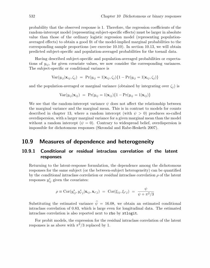
. quietly xtset patient
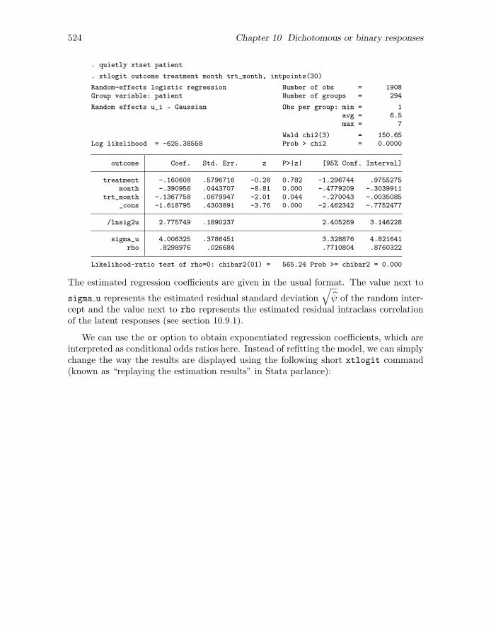
. xtlogit outcome treatment month trt_month, intpoints(30)
Random-effects logistic regression Number of obs = 1908Group variable: patient Number of groups = 294
Random effects u_i ~ Gaussian Obs per group: min = 1avg = 6.5max = 7
Wald chi2(3) = 150.65Log likelihood = -625.38558 Prob > chi2 = 0.0000
outcome Coef. Std. Err. z P>|z| [95% Conf. Interval]
treatment -.160608 .5796716 -0.28 0.782 -1.296744 .9755275month -.390956 .0443707 -8.81 0.000 -.4779209 -.3039911
trt_month -.1367758 .0679947 -2.01 0.044 -.270043 -.0035085_cons -1.618795 .4303891 -3.76 0.000 -2.462342 -.7752477
/lnsig2u 2.775749 .1890237 2.405269 3.146228
sigma_u 4.006325 .3786451 3.328876 4.821641rho .8298976 .026684 .7710804 .8760322
Likelihood-ratio test of rho=0: chibar2(01) = 565.24 Prob >= chibar2 = 0.000
The estimated regression coefficients are given in the usual format. The value next to
sigma u represents the estimated residual standard deviation
√ψ of the random inter-
cept and the value next to rho represents the estimated residual intraclass correlationof the latent responses (see section 10.9.1).
We can use the or option to obtain exponentiated regression coefficients, which areinterpreted as conditional odds ratios here. Instead of refitting the model, we can simplychange the way the results are displayed using the following short xtlogit command(known as “replaying the estimation results” in Stata parlance):

10.7.1 Using xtlogit 525
. xtlogit, or
Random-effects logistic regression Number of obs = 1908Group variable: patient Number of groups = 294
Random effects u_i ~ Gaussian Obs per group: min = 1avg = 6.5max = 7
Wald chi2(3) = 150.65Log likelihood = -625.38558 Prob > chi2 = 0.0000
outcome OR Std. Err. z P>|z| [95% Conf. Interval]
treatment .8516258 .4936633 -0.28 0.782 .2734207 2.652566month .6764099 .0300128 -8.81 0.000 .6200712 .7378675
trt_month .8721658 .0593027 -2.01 0.044 .7633467 .9964976_cons .1981373 .0852762 -3.76 0.000 .0852351 .4605897
/lnsig2u 2.775749 .1890237 2.405269 3.146228
sigma_u 4.006325 .3786451 3.328876 4.821641rho .8298976 .026684 .7710804 .8760322
Likelihood-ratio test of rho=0: chibar2(01) = 565.24 Prob >= chibar2 = 0.000
The estimated odds ratios and their 95% confidence intervals are also given in ta-ble 10.2. We see that the estimated conditional odds (given ζj) for a subject in theitraconazole group are multiplied by 0.68 every month and the conditional odds for asubject in the terbinafine group are multiplied by 0.59 (= 0.6764099× 0.8721658) everymonth. In terms of percentage change in estimated odds, 100%(OR − 1), the condi-tional odds decrease 32% [−32% = 100%(0.6764099− 1)] per month in the itraconazolegroup and 41% [−41% = 100%(0.6764099×0.8721658−1)] per month in the terbinafinegroup. (the difference between the kind of effects estimated in random-intercept logisticregression and ordinary logistic regression is discussed in section 10.8).

526 Chapter 10 Dichotomous or binary responses
Tab
le10
.2:
Est
imat
esfo
rto
enai
ldat
a
Mar
ginal
effec
tsC
ondit
ional
effec
tsO
rdin
ary
GE
E†
Ran
dom
int.
Con
dit
ional
logi
stic
logi
stic
logi
stic
logi
stic
Par
amet
erO
R(9
5%C
I)O
R(9
5%C
I)⋆
OR
(95%
CI)
OR
(95%
CI)
Fix
edpar
tex
p(β
2)
[treatment]
1.00
(0.7
4,1.
36)
1.01
(0.6
1,1.
68)
0.85
(0.2
7,2.
65)
exp(β
3)
[month]
0.84
(0.8
1,0.
88)
0.84
(0.7
9,0.
89)
0.68
(0.6
2,0.
74)
0.68
(0.6
2,0.
75)
exp(β
4)
[trtmonth]
0.93
(0.8
7,1.
01)
0.93
(0.8
3,1.
03)
0.87
(0.7
6,1.
00)
0.91
(0.7
8,1.
05)
Ran
dom
par
tψ
16.0
8ρ
0.83
Log
like
lihood
−90
8.01
−62
5.39
−18
8.94
•
†U
sing
exch
angea
ble
work
ing
corr
elati
on
⋆B
ase
don
the
sandw
ich
esti
mato
r•Log
condit
ionallikel
ihood

10.7.3 Using gllamm 527
10.7.2 Using xtmelogit
The syntax for xtmelogit is analogous to that for xtmixed except that we also specifythe number of quadrature points, or integration points, using the intpoints() option
. xtmelogit outcome treatment month trt_month || patient:, intpoints(30)
Mixed-effects logistic regression Number of obs = 1908Group variable: patient Number of groups = 294
Obs per group: min = 1avg = 6.5max = 7
Integration points = 30 Wald chi2(3) = 150.52Log likelihood = -625.39709 Prob > chi2 = 0.0000
outcome Coef. Std. Err. z P>|z| [95% Conf. Interval]
treatment -.1609377 .584208 -0.28 0.783 -1.305964 .984089month -.3910603 .0443957 -8.81 0.000 -.4780744 -.3040463
trt_month -.1368073 .0680236 -2.01 0.044 -.270131 -.0034836_cons -1.618961 .4347772 -3.72 0.000 -2.471108 -.7668132
Random-effects Parameters Estimate Std. Err. [95% Conf. Interval]
patient: Identitysd(_cons) 4.008164 .3813917 3.326216 4.829926
LR test vs. logistic regression: chibar2(01) = 565.22 Prob>=chibar2 = 0.0000
The results are similar but not identical to those from xtlogit because the commandsuse slightly different versions of adaptive quadrature (see section 10.11.1). Because theestimates took some time to obtain, we store them for later use within the same Statasession:
. estimates store xtmelogit
(The command estimates save can be used to save the estimates in a file for use in afuture Stata session.)
Estimated odds ratios can be obtained using the or option. xtmelogit can also beused with one integration point, which is equivalent to using the Laplace approximation.See section 10.11.2 for the results obtained by using this less accurate but faster methodfor the toenail data.
10.7.3 Using gllamm
We now introduce the user-contributed command for multilevel and latent variablemodeling, called gllamm (stands for generalized linear latent and mixed models) byRabe-Hesketh, Skrondal, and Pickles (2002, 2005). See also http://www.gllamm.orgwhere you can download the gllamm manual, the gllamm companion for this book, andfind many other resources.

528 Chapter 10 Dichotomous or binary responses
To check whether gllamm is installed on your computer, use the command
. which gllamm
If the message
command gllamm not found as either built-in or ado-file
appears, install gllamm (assuming that you have a net-aware Stata) by using the ssc
command:
. ssc install gllamm
Occasionally, you should update gllamm by using ssc with the replace option:
. ssc install gllamm, replace
Using gllamm for the random-intercept logistic regression model requires that wespecify a logit link and binomial distribution with the link() and family() options(exactly as for the glm command). We also use the nip() option (for the number ofintegration points) to request that 30 integration points be used. The cluster identifieris specified in the i() option:
. gllamm outcome treatment month trt_month, i(patient) link(logit) family(binomial)> nip(30) adapt
number of level 1 units = 1908number of level 2 units = 294
Condition Number = 23.0763
gllamm model
log likelihood = -625.38558
outcome Coef. Std. Err. z P>|z| [95% Conf. Interval]
treatment -.1608751 .5802054 -0.28 0.782 -1.298057 .9763066month -.3911055 .0443906 -8.81 0.000 -.4781096 -.3041015
trt_month -.136829 .0680213 -2.01 0.044 -.2701484 -.0035097_cons -1.620364 .4322409 -3.75 0.000 -2.46754 -.7731873
Variances and covariances of random effects------------------------------------------------------------------------------
***level 2 (patient)
var(1): 16.084107 (3.0626224)------------------------------------------------------------------------------
The estimates are again similar to those from xtlogit and xtmelogit. The es-timated random-intercept variance is given next to var(1) instead of the random-intercept standard deviation reported by xtlogit and xtmelogit, unless the varianceoption is used for the latter. We store the gllamm estimates for later use:

10.8 Subject-specific vs. population-averaged relationships 529
. estimates store gllamm
We can use the eform option to obtain estimated odds ratios, or we can alternativelyuse the command
gllamm, eform
to replay the estimation results after having already fit the model. We can also use therobust option to obtain robust standard errors based on the sandwich estimator. Atthe time of writing this book, gllamm does not accept factor variables (i., c., and #)but does accept i. if the gllamm command is preceded by the prefix command xi:.
10.8 Subject-specific or conditional vs.
population-averaged or marginal relationships
The estimated regression coefficients for the random-intercept logistic regression modelare more extreme (more different from 0) than those for the ordinary logistic regressionmodel (see table 10.2). Correspondingly, the estimated odds ratios are more extreme(more different from 1) than those for the ordinary logistic regression model. The reasonfor this discrepancy is that ordinary logistic regression fits overall population-averagedor marginal probabilities, whereas random-effects logistic regression fits subject-specificor conditional probabilities for the individual patients.
This important distinction can be seen in the way the two models are writtenin (10.5) and (10.6). Whereas the former is for the overall or population-averaged prob-ability, conditioning only on covariates, the latter is for the subject-specific probability,given the subject-specific random intercept ζj and the covariates. Odds ratios derivedfrom these models can be referred to as population-averaged (although the averaging isapplied to the probabilities) or subject-specific odds ratios, respectively.
For instance, in the random-intercept logistic regression model, we can interpret theestimated subject-specific or conditional odds ratio of 0.68 for month (a covariate varyingwithin patient) as the odds ratio for each patient in the itraconazole group: the odds for agiven patient hence decreases by 32% per month. In contrast, the estimated population-averaged odds ratio of 0.84 for month means that the odds of having onycholysis amongthe patients in the itraconazole group decreases by 16% per month.
Considering instead the odds for treatment (a covariate only varying between pa-tients) when month equals 1, the estimated subject-specific or conditional odds ratiois estimated as 0.74 (=0.85×0.87) and the odds are hence 26% lower for terbinafinethan for itraconazole for each subject. However, because no patients are given bothterbinafine and itraconazole, it might be best to interpret the odds ratio in terms of acomparison between two patients j and j′ with the same value of the random interceptζj = ζj′ , one of whom is given terbinafine and the other itraconazole. The estimatedpopulation-averaged or marginal odds ratio of about 0.93 (=1.00×0.93) means that theodds are 7% lower for the group of patients given terbinafine compared with the groupof patients given itraconazole.
530 Chapter 10 Dichotomous or binary responses
When interpreting subject-specific or conditional odds ratios, keep in mind thatthese are not purely based on within-subject information and are hence not free fromsubject-level confounding. In fact, for between-subject covariates like treatment groupabove, there is no within-subject information in the data. Although the odds ratios areinterpreted as effects keeping the subject-specific random intercepts ζj constant, theserandom intercepts are assumed to be independent of the covariates included in the modeland hence do not represent effects of unobserved confounders, which are by definitioncorrelated with the covariates. Unlike fixed-effects approaches, we are therefore notcontrolling for unobserved confounders. Both conditional and marginal effect estimatessuffer from omitted-variable bias if subject-level or other confounders are not includedin the model. See section 3.7.4 for a discussion of this issue in linear random-interceptmodels. Section 10.14.1 is on conditional logistic regression, the fixed-effects approachin logistic regression that controls for subject-level confounders.
The population-averaged probabilities implied by the random-intercept model canbe obtained by averaging the subject-specific probabilities over the random-interceptdistribution. Because the random intercepts are continuous, this averaging is accom-plished by integration
Pr(yij = 1|x2j , x3ij)
=
∫Pr(yij = 1|x2j , x3ij , ζj)φ(ζj ; 0, ψ) dζj
=
∫exp(β1 + β2x2j + β3x3ij + β4x2jx3ij + ζj)
1 + exp(β1 + β2x2j + β3x3ij + β4x2jx3ij + ζj)φ(ζj ; 0, ψ) dζj
6= exp(β1 + β2x2j + β3x3ij + β4x2jx3ij)
1 + exp(β1 + β2x2j + β3x3ij + β4x2jx3ij)(10.8)
where φ(ζj ; 0, ψ) is the normal density function with mean zero and variance ψ.
The difference between population-averaged and subject-specific effects is due tothe average of a nonlinear function not being the same as the nonlinear function of theaverage. In the present context, the average of the inverse logit of the linear predictor,β1 + β2x2j + β3x3ij + β4x2jx3ij + ζj , is not the same as the inverse logit of the averageof the linear predictor, which is β1 + β2x2j + β3x3ij + β4x2jx3ij . We can see this bycomparing the simple average of the logits of 1 and 2 with the logit of the average of 1and 2:
. display (invlogit(1) + invlogit(2))/2
.80592783
. display invlogit((1+2)/1)
.95257413
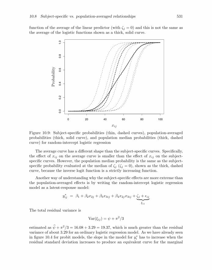
We can also see this in figure 10.9. Here the individual, thin, dashed curves representsubject-specific logistic curves, each with a subject-specific (randomly drawn) intercept.These are inverse logit functions of the subject-specific linear predictors (here the linearpredictors are simply β1 + β2xij + ζj). The thick, dashed curve is the inverse logit
10.8 Subject-specific vs. population-averaged relationships 531
function of the average of the linear predictor (with ζj = 0) and this is not the same asthe average of the logistic functions shown as a thick, solid curve.
0 20 40 60 80 100
0.0
0.2
0.4
0.6
0.8
1.0
Pro
bab
ility
xij
Figure 10.9: Subject-specific probabilities (thin, dashed curves), population-averagedprobabilities (thick, solid curve), and population median probabilities (thick, dashedcurve) for random-intercept logistic regression
The average curve has a different shape than the subject-specific curves. Specifically,the effect of xij on the average curve is smaller than the effect of xij on the subject-specific curves. However, the population median probability is the same as the subject-specific probability evaluated at the median of ζj (ζj = 0), shown as the thick, dashedcurve, because the inverse logit function is a strictly increasing function.
Another way of understanding why the subject-specific effects are more extreme thanthe population-averaged effects is by writing the random-intercept logistic regressionmodel as a latent-response model:
y∗ij = β1 + β2x2j + β3x3ij + β4x2jx3ij + ζj + ǫij︸ ︷︷ ︸ξij
The total residual variance is
Var(ξij) = ψ + π2/3
estimated as ψ + π2/3 = 16.08 + 3.29 = 19.37, which is much greater than the residualvariance of about 3.29 for an ordinary logistic regression model. As we have already seenin figure 10.4 for probit models, the slope in the model for y∗i has to increase when theresidual standard deviation increases to produce an equivalent curve for the marginal
532 Chapter 10 Dichotomous or binary responses
probability that the observed response is 1. Therefore, the regression coefficients of therandom-intercept model (representing subject-specific effects) must be larger in absolutevalue than those of the ordinary logistic regression model (representing population-averaged effects) to obtain a good fit of the model-implied marginal probabilities to thecorresponding sample proportions (see exercise 10.10). In section 10.13, we will obtainpredicted subject-specific and population-averaged probabilities for the toenail data.
Having described subject-specific and population-averaged probabilities or expecta-tions of yij , for given covariate values, we now consider the corresponding variances.The subject-specific or conditional variance is
Var(yij |xij , ζj) = Pr(yij = 1|xij , ζj){1 − Pr(yij = 1|xij , ζj)}
and the population-averaged or marginal variance (obtained by integrating over ζj) is
Var(yij |xij) = Pr(yij = 1|xij){1 − Pr(yij = 1|xij)}
We see that the random-intercept variance ψ does not affect the relationship betweenthe marginal variance and the marginal mean. This is in contrast to models for countsdescribed in chapter 13, where a random intercept (with ψ > 0) produces so-calledoverdispersion, with a larger marginal variance for a given marginal mean than the modelwithout a random intercept (ψ = 0). Contrary to widespread belief, overdispersion isimpossible for dichotomous responses (Skrondal and Rabe-Hesketh 2007).
10.9 Measures of dependence and heterogeneity
10.9.1 Conditional or residual intraclass correlation of the latentresponses
Returning to the latent-response formulation, the dependence among the dichotomousresponses for the same subject (or the between-subject heterogeneity) can be quantifiedby the conditional intraclass correlation or residual intraclass correlation ρ of the latentresponses y∗ij given the covariates:
ρ ≡ Cor(y∗ij , y∗i′j |xij ,xi′j) = Cor(ξij , ξi′j) =
ψ
ψ + π2/3
Substituting the estimated variance ψ = 16.08, we obtain an estimated conditionalintraclass correlation of 0.83, which is large even for longitudinal data. The estimatedintraclass correlation is also reported next to rho by xtlogit.
For probit models, the expression for the residual intraclass correlation of the latentresponses is as above with π2/3 replaced by 1.
10.9.3 q Measures of association for observed responses 533
10.9.2 Median odds ratio
Larsen et al. (2000) and Larsen and Merlo (2005) suggest a measure of heterogeneity forrandom-intercept models with normally distributed random intercepts. They considerrepeatedly sampling two subjects with the same covariate values and forming the oddsratio comparing the subject who has the larger random intercept with the other subject.For a given pair of subjects j and j′, this odds ratio is given by exp(|ζj − ζj′ |) andheterogeneity is expressed as the median of these odds ratios across repeated samples.
The median and other percentiles a > 1 can be obtained from the cumulative dis-tribution function
Pr{exp(|ζj − ζj′ |) ≤ a} = Pr
{ |ζj − ζj′ |√2ψ
≤ ln(a)√2ψ
}= 2Φ
{ln(a)√
2ψ
}− 1
If the cumulative probability is set to 1/2, a is the median odds ratio, ORmedian:
2Φ
{ln(ORmedian)√
2ψ
}− 1 = 1/2
Solving this equation gives
ORmedian = exp{√
2ψΦ−1(3/4)}
Plugging in the parameter estimates, we obtain ORmedian:
. display exp(sqrt(2*16.084107)*invnormal(3/4))45.855974
When two subjects are chosen at random at a given time point from the same treatmentgroup, the odds ratio comparing the subject who has the larger odds with the subjectwho has the smaller odds will exceed 45.83 half the time, which is a very large oddsratio. For comparison, the estimated odds ratio comparing two subjects at 20 monthswho had the same value of the random intercept, but one of whom received itraconazole(treatment=0) and the other of whom received terbinafine (treatment=1), is about18 {= 1/ exp(−0.1608751 + 20 ×−0.136829)}.
10.9.3 qMeasures of association for observed responses at median fixedpart of the model
The reason why the degree of dependence is often expressed in terms of the residualintraclass correlation for the latent responses y∗ij is that the intraclass correlation forthe observed responses yij varies according to the values of the covariates.
One may nevertheless proceed by obtaining measures of association for specific val-ues of the covariates. In particular, Rodrıguez and Elo (2003) suggest obtaining themarginal association between the binary observed responses at the sample median value
534 Chapter 10 Dichotomous or binary responses
of the estimated fixed part of the model, β1 + β2x2j + β3x3ij + β4x2jx3ij . Marginal asso-ciation here refers to the fact that the associations are based on marginal probabilities(averaged over the random-intercept distribution with the maximum likelihood estimate
ψ plugged in).
Rodrıguez and Elo (2003) have written a program called xtrho that can be usedafter xtlogit, xtprobit, and xtclog to produce such marginal association measuresand their confidence intervals. The program can be downloaded by issuing the command
. findit xtrho
clicking on st0031, and then clicking on click here to install. Having downloadedxtrho, we run it after refitting the random-intercept logistic model with xtlogit:
. quietly xtset patient
. quietly xtlogit outcome treatment month trt_month, re intpoints(30)
. xtrho
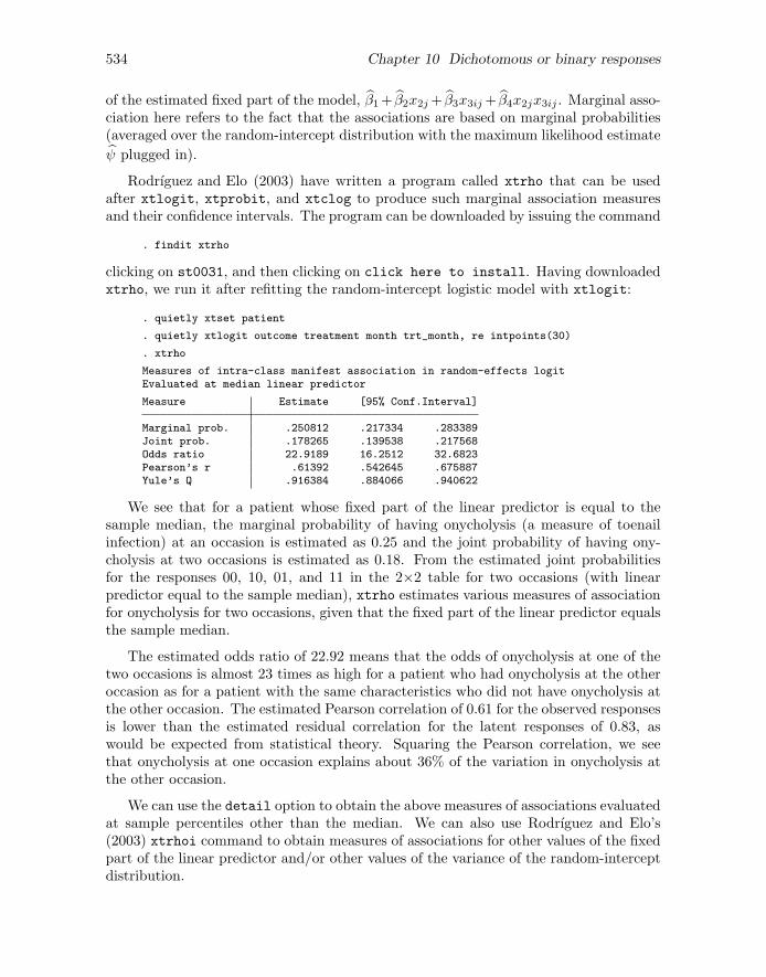
Measures of intra-class manifest association in random-effects logitEvaluated at median linear predictor
Measure Estimate [95% Conf.Interval]
Marginal prob. .250812 .217334 .283389Joint prob. .178265 .139538 .217568Odds ratio 22.9189 16.2512 32.6823Pearson’s r .61392 .542645 .675887Yule’s Q .916384 .884066 .940622
We see that for a patient whose fixed part of the linear predictor is equal to thesample median, the marginal probability of having onycholysis (a measure of toenailinfection) at an occasion is estimated as 0.25 and the joint probability of having ony-cholysis at two occasions is estimated as 0.18. From the estimated joint probabilitiesfor the responses 00, 10, 01, and 11 in the 2×2 table for two occasions (with linearpredictor equal to the sample median), xtrho estimates various measures of associationfor onycholysis for two occasions, given that the fixed part of the linear predictor equalsthe sample median.
The estimated odds ratio of 22.92 means that the odds of onycholysis at one of thetwo occasions is almost 23 times as high for a patient who had onycholysis at the otheroccasion as for a patient with the same characteristics who did not have onycholysis atthe other occasion. The estimated Pearson correlation of 0.61 for the observed responsesis lower than the estimated residual correlation for the latent responses of 0.83, aswould be expected from statistical theory. Squaring the Pearson correlation, we seethat onycholysis at one occasion explains about 36% of the variation in onycholysis atthe other occasion.
We can use the detail option to obtain the above measures of associations evaluatedat sample percentiles other than the median. We can also use Rodrıguez and Elo’s(2003) xtrhoi command to obtain measures of associations for other values of the fixedpart of the linear predictor and/or other values of the variance of the random-interceptdistribution.
10.10.1 Tests and confidence intervals for odds ratios 535
Note that xtrho and xtrhoi assume that the fixed part of the linear predictor is thesame across occasions. However, in the toenail example, month must change betweenany two occasions within a patient, and the linear predictor is a function of month.Considering two occasions with month equal to 3 and 6, the odds ratio is estimated as25.6 for patients in the control group and 29.4 for patients in the treatment group. Ado-file that produces the 2×2 tables by using gllamm and gllapred with the ll optioncan be copied into the working directory with the command
copy http://www.stata-press.com/data/mlmus3/ch10table.do ch10table.do
10.10 Inference for random-intercept logistic models
10.10.1 Tests and confidence intervals for odds ratios
As discussed earlier, we can interpret the regression coefficient β as the difference in logodds associated with a unit change in the corresponding covariate, and we can interpretthe exponentiated regression coefficient as an odds ratio, OR = exp(β). The relevantnull hypothesis for odds ratios usually is H0: OR = 1, and this corresponds directly tothe null hypothesis that the corresponding regression coefficient is zero, H0: β = 0.
Wald tests and z tests can be used for regression coefficients just as described in sec-tion 3.6.1 for linear models. Ninety-five percent Wald confidence intervals for individualregression coefficients are obtained using
β ± z0.975 SE(β)
where z0.975 = 1.96 is the 97.5th percentile of the standard normal distribution. Thecorresponding confidence interval for the odds ratio is obtained by exponentiating bothlimits of the confidence interval:
exp{β − z0.975 SE(β)} to exp{β + z0.975 SE(β)}
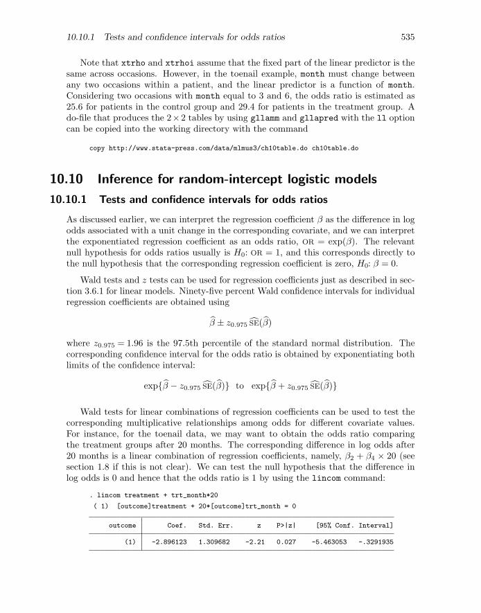
Wald tests for linear combinations of regression coefficients can be used to test thecorresponding multiplicative relationships among odds for different covariate values.For instance, for the toenail data, we may want to obtain the odds ratio comparingthe treatment groups after 20 months. The corresponding difference in log odds after20 months is a linear combination of regression coefficients, namely, β2 + β4 × 20 (seesection 1.8 if this is not clear). We can test the null hypothesis that the difference inlog odds is 0 and hence that the odds ratio is 1 by using the lincom command:
. lincom treatment + trt_month*20
( 1) [outcome]treatment + 20*[outcome]trt_month = 0
outcome Coef. Std. Err. z P>|z| [95% Conf. Interval]
(1) -2.896123 1.309682 -2.21 0.027 -5.463053 -.3291935

536 Chapter 10 Dichotomous or binary responses
If we require the corresponding odds ratio with a 95% confidence interval, we can usethe lincom command with the or option:
. lincom treatment + trt_month*20, or
( 1) [outcome]treatment + 20*[outcome]trt_month = 0
outcome Odds Ratio Std. Err. z P>|z| [95% Conf. Interval]
(1) .0552369 .0723428 -2.21 0.027 .0042406 .7195038
After 20 months of treatment, the odds ratio comparing terbinafine (treatment=1) withitraconazole is estimated as 0.055. Such small numbers are difficult to interpret, so wecan switch the groups around by taking the reciprocal of the odds ratio, 18 (= 1/0.055),which represents the odds ratio comparing itraconazole with terbinafine. Alternatively,we can always switch the comparison around by simply changing the sign of the corre-sponding difference in log odds in the lincom command:
lincom -(treatment + trt_month*20), or
If we had used factor-variable notation in the estimation command, using the syntaxi.treatment##c.month, then the lincom command above would have to be replacedwith
lincom -(1.treatment + 1.treatment#c.month*20), or
Multivariate Wald tests can be performed by using testparm. Wald tests and con-fidence intervals can be based on robust standard errors from the sandwich estimator.At the time of printing, robust standard errors can only be obtained using gllamm withthe robust option.
Null hypotheses about individual regression coefficients or several regression coeffi-cients can also be tested using likelihood-ratio tests. Although likelihood-ratio and Waldtests are asymptotically equivalent, the test statistics are not identical in finite samples.(See display 2.1 for the relationships between likelihood-ratio, Wald, and score tests.)If the statistics are very different, there may be a sparseness problem, for instance withmostly “1” responses or mostly “0” responses in one of the groups.
10.10.2 Tests of variance components
Both xtlogit and xtmelogit provide likelihood-ratio tests for the null hypothesis thatthe residual between-cluster variance ψ is zero in the last line of the output. The p-values are based on the correct asymptotic sampling distribution (not the naıve χ2
1), asdescribed for linear models in section 2.6.2. For the toenail data, the likelihood-ratiostatistic is 565.2 giving p < 0.001, which suggests that a multilevel model is required.
10.11.1 q Adaptive quadrature 537
10.11 Maximum likelihood estimation
10.11.1 q Adaptive quadrature
The marginal likelihood is the joint probability of all observed responses given theobserved covariates. For linear mixed models, this marginal likelihood can be evaluatedand maximized relatively easily (see section 2.10). However, in generalized linear mixedmodels, the marginal likelihood does not have a closed form and must be evaluated byapproximate methods.
To see this, we will now construct this marginal likelihood step by step for a random-intercept logistic regression model with one covariate xj . The responses are conditionallyindependent given the random intercept ζj and the covariate xj . Therefore, the jointprobability of all the responses yij (i = 1, . . . , nj) for cluster j given the random interceptand covariate is simply the product of the conditional probabilities of the individualresponses:
Pr(y1j , . . . , ynjj |xj , ζj) =
nj∏
i=1
Pr(yij |xj , ζj) =
nj∏
i=1
exp(β1 + β2xj + ζj)yij
1 + exp(β1 + β2xj + ζj)
In the last term
exp(β1 + β2xj + ζj)yij
1 + exp(β1 + β2xj + ζj)=
exp(β1+β2xj+ζj)1+exp(β1+β2xj+ζj)
if yij = 1
11+exp(β1+β2xj+ζj)
if yij = 0
as specified by the logistic regression model.
To obtain the marginal joint probability of the responses, not conditioning on therandom intercept ζj (but still on the covariate xj), we integrate out the random intercept
Pr(y1j , . . . , ynjj |xj) =
∫Pr(y1j , . . . , ynjj |xj , ζj)φ(ζj ; 0, ψ) dζj (10.9)
where φ(ζj , 0, ψ) is the normal density of ζj with mean 0 and variance ψ. Unfortunately,this integral does not have a closed-form expression.
The marginal likelihood is just the joint probability of all responses for all clusters.Because the clusters are mutually independent, this is given by the product of themarginal joint probabilities of the responses for the individual clusters
L(β1, β2, ψ) =
N∏
j=1
Pr(y1j , . . . , ynjj |xj)
This marginal likelihood is viewed as a function of the parameters β1, β2, and ψ (withthe observed responses treated as given). The parameters are estimated by finding thevalues of β1, β2, and ψ that yield the largest likelihood. The search for the maximum isiterative, beginning with some initial guesses or starting values for the parameters and
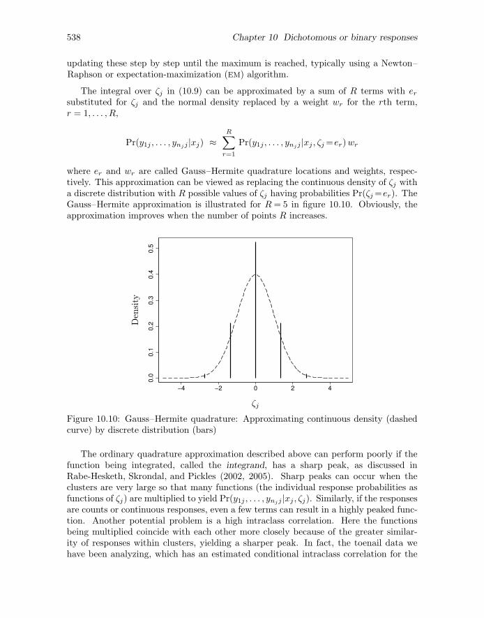
538 Chapter 10 Dichotomous or binary responses
updating these step by step until the maximum is reached, typically using a Newton–Raphson or expectation-maximization (EM) algorithm.
The integral over ζj in (10.9) can be approximated by a sum of R terms with er
substituted for ζj and the normal density replaced by a weight wr for the rth term,r = 1, . . . , R,
Pr(y1j , . . . , ynjj |xj) ≈R∑
r=1
Pr(y1j , . . . , ynjj |xj , ζj =er)wr
where er and wr are called Gauss–Hermite quadrature locations and weights, respec-tively. This approximation can be viewed as replacing the continuous density of ζj witha discrete distribution with R possible values of ζj having probabilities Pr(ζj =er). TheGauss–Hermite approximation is illustrated for R= 5 in figure 10.10. Obviously, theapproximation improves when the number of points R increases.
0.0
0.1
0.2
0.3
0.4
0.5
−4 −2 0 2 4
ζj
Den
sity
Figure 10.10: Gauss–Hermite quadrature: Approximating continuous density (dashedcurve) by discrete distribution (bars)
The ordinary quadrature approximation described above can perform poorly if thefunction being integrated, called the integrand, has a sharp peak, as discussed inRabe-Hesketh, Skrondal, and Pickles (2002, 2005). Sharp peaks can occur when theclusters are very large so that many functions (the individual response probabilities asfunctions of ζj) are multiplied to yield Pr(y1j , . . . , ynjj |xj , ζj). Similarly, if the responsesare counts or continuous responses, even a few terms can result in a highly peaked func-tion. Another potential problem is a high intraclass correlation. Here the functionsbeing multiplied coincide with each other more closely because of the greater similar-ity of responses within clusters, yielding a sharper peak. In fact, the toenail data wehave been analyzing, which has an estimated conditional intraclass correlation for the
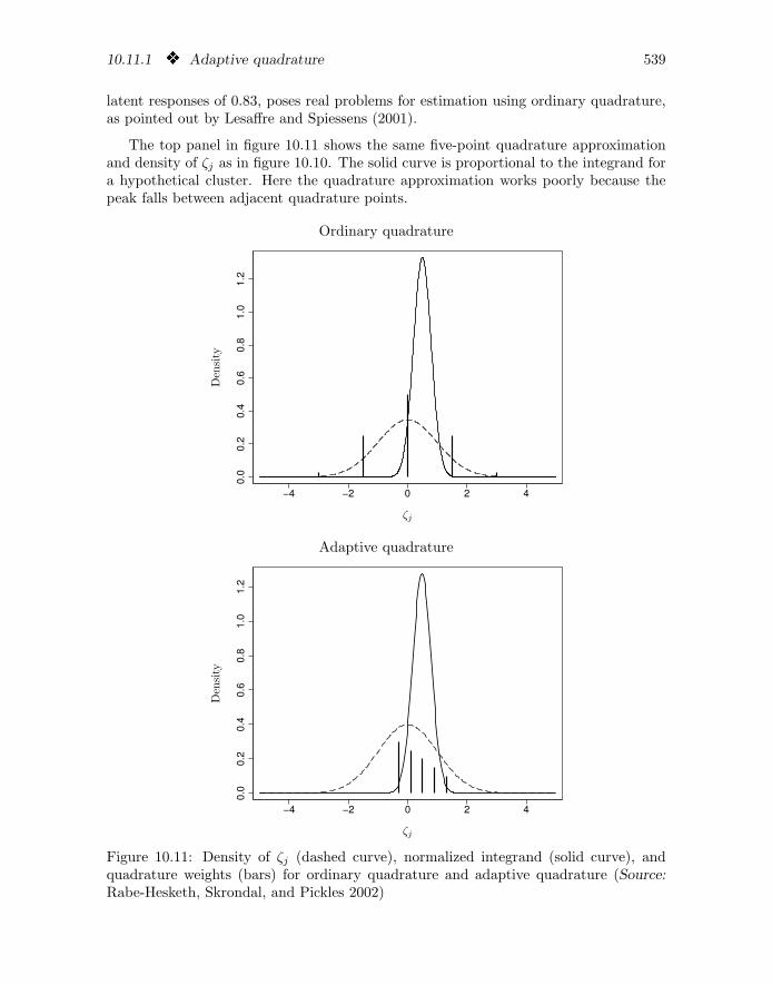
10.11.1 q Adaptive quadrature 539
latent responses of 0.83, poses real problems for estimation using ordinary quadrature,as pointed out by Lesaffre and Spiessens (2001).
The top panel in figure 10.11 shows the same five-point quadrature approximationand density of ζj as in figure 10.10. The solid curve is proportional to the integrand fora hypothetical cluster. Here the quadrature approximation works poorly because thepeak falls between adjacent quadrature points.
Ordinary quadrature0.0
0.2
0.4
0.6
0.8
1.0
1.2
−4 −2 0 2 4
Den
sity
ζj
Adaptive quadrature
0.0
0.2
0.4
0.6
0.8
1.0
1.2
−4 −2 0 2 4
Den
sity
ζj
Figure 10.11: Density of ζj (dashed curve), normalized integrand (solid curve), andquadrature weights (bars) for ordinary quadrature and adaptive quadrature (Source:Rabe-Hesketh, Skrondal, and Pickles 2002)
540 Chapter 10 Dichotomous or binary responses
The bottom panel of figure 10.11 shows an improved approximation, known as adaptivequadrature, where the locations are rescaled and translated,
erj = aj + bjer (10.10)
to fall under the peak of the integrand, where aj and bj are cluster-specific constants.This transformation of the locations is accompanied by a transformation of the weightswr that also depends on aj and bj . The method is called adaptive because the quadra-ture locations and weights are adapted to the data for the individual clusters.
To maximize the likelihood, we start with a set of initial or starting values of theparameters and then keep updating the parameters until the likelihood is maximized.The quantities aj and bj needed to evaluate the likelihood are functions of the param-eters (as well as the data) and must therefore be updated or “readapted” when theparameters are updated.
There are two different implementations of adaptive quadrature in Stata that differin the values used for aj and bj in (10.10). The method implemented in gllamm, whichis the default method in xtlogit (as of Stata 10), uses the posterior mean of ζj for aj
and the posterior standard deviation for bj . However, obtaining the posterior mean andstandard deviation requires numerical integration so adaptive quadrature sometimesdoes not work when there are too few quadrature points (for example, fewer than five).Details of the algorithm are given in Rabe-Hesketh, Skrondal, and Pickles (2002, 2005)and Skrondal and Rabe-Hesketh (2004).
The method implemented in xtmelogit, and available in xtlogit with the optionintmethod(aghermite), uses the posterior mode of ζj for aj and for bj uses the standarddeviation of the normal density that approximates the log posterior of ζj at the mode.An advantage of this approach is that it does not rely on numerical integration and cantherefore be implemented even with one quadrature point. With one quadrature point,this version of adaptive quadrature becomes a Laplace approximation.
10.11.2 Some speed and accuracy considerations
As discussed in section 10.11.1, the likelihood involves integrals that are evaluated by nu-merical integration. The likelihood itself, as well as the maximum likelihood estimates,are therefore only approximate. The accuracy increases as the number of quadraturepoints increases, at the cost of increased computation time. We can assess whetherthe approximation is adequate in a given situation by repeating the analysis with alarger number of quadrature points. If we get essentially the same result, the lowernumber of quadrature points is likely to be adequate. Such checking should always bedone before estimates are taken at face value. See section 16.4.1 for an example ingllamm and section 16.4.2 for an example in xtmelogit. For a given number of quadra-ture points, adaptive quadrature is more accurate than ordinary quadrature. Stata’scommands therefore use adaptive quadrature by default, and we recommend using theadapt option in gllamm.

10.11.2 Some speed and accuracy considerations 541
Because of numerical integration, estimation can be slow, especially if there are manyrandom effects. The time it takes to fit a model is approximately proportional to theproduct of the number of quadrature points for all random effects (although this seemsto be more true for gllamm than for xtmelogit). For example, if there are two randomeffects at level 2 (a random intercept and slope) and eight quadrature points are used foreach random effect, the time will be approximately proportional to 64. Therefore, usingfour quadrature points for each random effect will take only about one-fourth (16/64)as long as using eight. The time is also approximately proportional to the number ofobservations and, for programs using numerical differentiation (gllamm and xtmelogit),to the square of the number of parameters. (For xtlogit, computation time increasesless dramatically when the number of parameters increases because it uses analyticalderivatives.)
For large problems, it may be advisable to estimate how long estimation will takebefore starting work on a project. In this case, we recommend fitting a similar modelwith fewer random effects, fewer parameters (for example, fewer covariates), or fewerobservations, and then using the above approximate proportionality factors to estimatethe time that will be required for the larger problem.
For random-intercept models, by far the fastest command is xtlogit (because ituses analytical derivatives). However, xtlogit cannot fit random-coefficient models orhigher-level models introduced in chapter 16. For such models, xtmelogit or gllamm
must be used. The quickest way of obtaining results here is using xtmelogit with oneintegration point, corresponding to the Laplace approximation. Although this methodsometimes works well, it can produce severely biased estimates, especially if the clustersare small and the (true) random-intercept variance is large, as for the toenail data. Forthese data, we obtain the following:
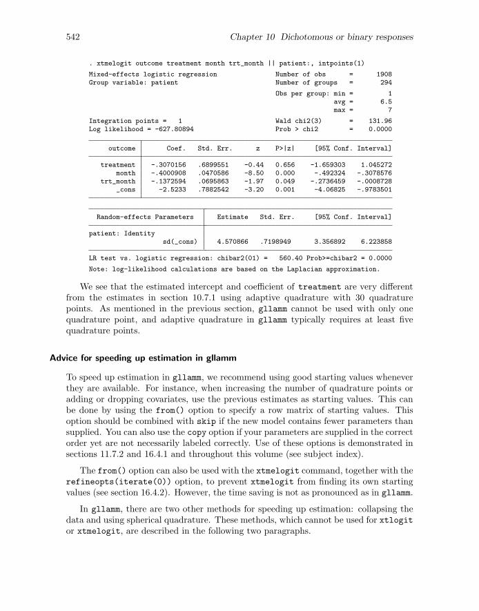
542 Chapter 10 Dichotomous or binary responses
. xtmelogit outcome treatment month trt_month || patient:, intpoints(1)
Mixed-effects logistic regression Number of obs = 1908Group variable: patient Number of groups = 294
Obs per group: min = 1avg = 6.5max = 7
Integration points = 1 Wald chi2(3) = 131.96Log likelihood = -627.80894 Prob > chi2 = 0.0000
outcome Coef. Std. Err. z P>|z| [95% Conf. Interval]
treatment -.3070156 .6899551 -0.44 0.656 -1.659303 1.045272month -.4000908 .0470586 -8.50 0.000 -.492324 -.3078576
trt_month -.1372594 .0695863 -1.97 0.049 -.2736459 -.0008728_cons -2.5233 .7882542 -3.20 0.001 -4.06825 -.9783501
Random-effects Parameters Estimate Std. Err. [95% Conf. Interval]
patient: Identitysd(_cons) 4.570866 .7198949 3.356892 6.223858
LR test vs. logistic regression: chibar2(01) = 560.40 Prob>=chibar2 = 0.0000
Note: log-likelihood calculations are based on the Laplacian approximation.
We see that the estimated intercept and coefficient of treatment are very differentfrom the estimates in section 10.7.1 using adaptive quadrature with 30 quadraturepoints. As mentioned in the previous section, gllamm cannot be used with only onequadrature point, and adaptive quadrature in gllamm typically requires at least fivequadrature points.
Advice for speeding up estimation in gllamm
To speed up estimation in gllamm, we recommend using good starting values wheneverthey are available. For instance, when increasing the number of quadrature points oradding or dropping covariates, use the previous estimates as starting values. This canbe done by using the from() option to specify a row matrix of starting values. Thisoption should be combined with skip if the new model contains fewer parameters thansupplied. You can also use the copy option if your parameters are supplied in the correctorder yet are not necessarily labeled correctly. Use of these options is demonstrated insections 11.7.2 and 16.4.1 and throughout this volume (see subject index).
The from() option can also be used with the xtmelogit command, together with therefineopts(iterate(0)) option, to prevent xtmelogit from finding its own startingvalues (see section 16.4.2). However, the time saving is not as pronounced as in gllamm.
In gllamm, there are two other methods for speeding up estimation: collapsing thedata and using spherical quadrature. These methods, which cannot be used for xtlogitor xtmelogit, are described in the following two paragraphs.
10.12 Assigning values to random effects 543
For some datasets and models, you can represent the data using fewer rows thanthere are observations, thus speeding up estimation. For example, if the response isdichotomous and we are using one dichotomous covariate in a two-level dataset, wecan use one row of data for each combination of covariate and response (00, 01, 10,11) for each cluster, leading to at most four rows per cluster. We can then specify avariable containing level-1 frequency weights equal to the number of observations, orlevel-1 units, in each cluster having each combination of the covariate and responsevalues. Level-2 weights can be used if several clusters have the same level-2 covariatesand the same number of level-1 units with the same response and level-1 covariatepattern. The weight() option in gllamm is designed for specifying frequency weightsat the different levels. See exercise 10.7 for an example with level-1 weights, and seeexercises 10.3 and 2.3 for examples with level-2 weights. In exercise 16.11, collapsingthe data reduces computation time by about 99%. If the dataset is large, starting valuescould be obtained by fitting the model to a random sample of the data.
For models involving several random effects at the same level, such as two-levelrandom-coefficient models with a random intercept and slope, the multivariate inte-gral can be evaluated more efficiently using spherical quadrature instead of the defaultCartesian-product quadrature. For the random intercept and slope example, Cartesian-product quadrature consists of evaluating the function being integrated on the rectan-gular grid of quadrature points consisting of all combinations of ζ1j = e1, . . . , eR andζ2j = e1, . . . , eR, giving R2 terms. In contrast, spherical quadrature consists of evalu-ating ζ1j and ζ2j at values falling on concentric circles (spheres in more dimensions).The important point is that the same accuracy can now be achieved with fewer thanR2 points. For example, when R = 8, Cartesian-product quadrature requires 64 evalu-ations, while spherical quadrature requires only 44 evaluations, taking nearly 30% lesstime to achieve the same accuracy. Here accuracy is expressed in terms of the degree ofthe approximation given by d = 2R−1. For R = 8, d = 15. To use spherical quadrature,specify the ip(m) option in gllamm and give the degree d of the approximation by usingthe nip(#) option. Unfortunately, spherical integration is available only for certaincombinations of numbers of dimensions (or numbers of random effects) and degrees ofaccuracy, d: For two dimensions, d can be 5, 7, 9, 11, or 15, and for more than twodimensions, d can be 5 or 7. See Rabe-Hesketh, Skrondal, and Pickles (2005) for moreinformation.
10.12 Assigning values to random effects
Having estimated the model parameters (the β’s and ψ), we may want to assign valuesto the random intercepts ζj for individual clusters j. The ζj are not model parameters,but as for linear models, we can treat the estimated parameters as known and theneither estimate or predict ζj .
Such predictions are useful for making inferences for the clusters in the data, im-portant examples being assessment of institutional performance (see section 4.8.5) or ofabilities in item response theory (see exercise 10.4). The estimated or predicted values
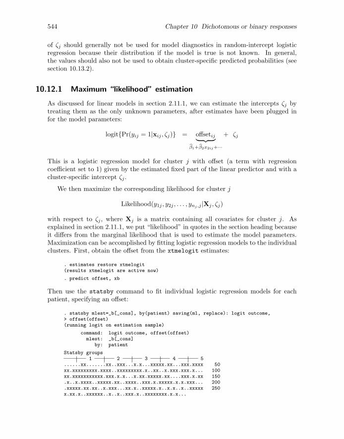
544 Chapter 10 Dichotomous or binary responses
of ζj should generally not be used for model diagnostics in random-intercept logisticregression because their distribution if the model is true is not known. In general,the values should also not be used to obtain cluster-specific predicted probabilities (seesection 10.13.2).
10.12.1 Maximum “likelihood” estimation
As discussed for linear models in section 2.11.1, we can estimate the intercepts ζj bytreating them as the only unknown parameters, after estimates have been plugged infor the model parameters:
logit{Pr(yij = 1|xij , ζj)} = offsetij︸ ︷︷ ︸bβ1+bβ2x2ij+···
+ ζj
This is a logistic regression model for cluster j with offset (a term with regressioncoefficient set to 1) given by the estimated fixed part of the linear predictor and with acluster-specific intercept ζj .
We then maximize the corresponding likelihood for cluster j
Likelihood(y1j , y2j , . . . , ynj ,j |Xj , ζj)
with respect to ζj , where Xj is a matrix containing all covariates for cluster j. Asexplained in section 2.11.1, we put “likelihood” in quotes in the section heading becauseit differs from the marginal likelihood that is used to estimate the model parameters.Maximization can be accomplished by fitting logistic regression models to the individualclusters. First, obtain the offset from the xtmelogit estimates:
. estimates restore xtmelogit(results xtmelogit are active now)
. predict offset, xb
Then use the statsby command to fit individual logistic regression models for eachpatient, specifying an offset:
. statsby mlest=_b[_cons], by(patient) saving(ml, replace): logit outcome,> offset(offset)(running logit on estimation sample)
command: logit outcome, offset(offset)mlest: _b[_cons]
by: patient
Statsby groups1 2 3 4 5
......xx.......xx..xxx...x.x...xxxxx.xx...xxx.xxxx 50xx.xxxxxxxxx.xxxx..xxxxxxxxx.x..xx..x.xxx.xxx.x... 100xx.xxxxxxxxxxx.xxx.x.x...x.xx.xxxxx.xx....xxx.x.xx 150.x..x.xxxx..xxxxx.xx..xxxx..xxx.x.xxxxx.x.x.xxx... 200.xxxxx.xx.xx..x.xxx...xx.x..xxxxx.x..x.x..x..xxxxx 250x.xx.x..xxxxxx..x..x..xxx.x..xxxxxxxx.x.x...
10.12.2 Empirical Bayes prediction 545
Here we have saved the estimates under the variable name mlest in a file called ml.dta
in the local directory. The x’s in the output indicate that the logit command didnot converge for many clusters. For these clusters, the variable mlest is missing. Thishappens for clusters where all responses are 0 or all responses are 1 because the maximumlikelihood estimate then is −∞ and +∞, respectively.
We now merge the estimates with the data for later use:
. sort patient
. merge m:1 patient using ml
. drop _merge
10.12.2 Empirical Bayes prediction
The ideas behind empirical Bayes prediction discussed in section 2.11.2 for linearvariance-components models also apply to other generalized linear mixed models. In-stead of basing inference completely on the likelihood of the responses for a clustergiven the random intercept, we combine this information with the prior of the randomintercept, which is just the density of the random intercept (a normal density with mean
0 and estimated variance ψ), to obtain the posterior density:
Posterior(ζj |y1j , . . . , ynjj ,Xj) ∝ Prior(ζj) × Likelihood(y1j , . . . , ynjj |Xj , ζj)
The product on the right is proportional to, but not equal to, the posterior density.Obtaining the posterior density requires dividing this product by a normalizing constantthat can only be obtained by numerical integration. Note that the model parametersare treated as known, and estimates are plugged into the expression for the posterior,giving what is sometimes called an estimated posterior distribution.
The estimated posterior density is no longer normal as for linear models, and henceits mode does not equal its mean. There are therefore two different types of predictionswe could consider: the mean of the posterior and its mode. The first is undoubtedlythe most common and is referred to as empirical Bayes prediction [sometimes calledexpected a posterior (EAP) prediction], whereas the second is referred to as empiricalBayes modal prediction [sometimes called modal a posterior (MAP) prediction].
546 Chapter 10 Dichotomous or binary responses
The empirical Bayes prediction of the random intercept for a cluster j is the meanof the estimated posterior distribution of the random intercept. This can be obtainedas
ζj =
∫ζj Posterior(ζj |y1j , . . . , ynjj ,Xj) dζj
using numerical integration.
At the time of writing this book, the only Stata command that provides empiricalBayes predictions for generalized linear mixed models is the postestimation commandgllapred for gllamm with the u option:
. estimates restore gllamm
. gllapred eb, u
The variable ebm1 contains the empirical Bayes predictions. In the next section, we willproduce a graph of these predictions, together with maximum likelihood estimates andempirical Bayes modal predictions.
The posterior standard deviations produced by gllapred in the variable ebs1 rep-resent the conditional standard deviations of the prediction errors, given the observedresponses and treating the parameter estimates as known. The square of ebs1 is also theconditional mean squared error of the prediction, conditional on the observed responses.As in section 2.11.3, we refer to this standard error as the comparative standard errorbecause it can be used to make inferences regarding the random effects of individualclusters and to compare clusters.
We mentioned in section 2.11.3 that, for linear models, the posterior variance wasthe same as the unconditional mean squared error of prediction (MSEP). However, thisis not true for generalized linear mixed models not having an identity link, such as therandom-intercept logistic model discussed here.
There is also no longer an easy way to obtain the sampling standard deviationof the empirical Bayes predictions or diagnostic standard error (see section 2.11.3).The ustd option for standardized level-2 residuals therefore divides the empirical Bayes
predictions by an approximation for this standard deviation,
√ψ − ebs12 (see Skrondal
and Rabe-Hesketh [2004, 231–232] or Skrondal and Rabe-Hesketh [2009] for details).
10.12.3 Empirical Bayes modal prediction
Instead of basing prediction of random effects on the mean of the posterior distribution,we can use the mode. Such empirical Bayes modal predictions are easy to obtain usingthe predict command with the reffects option after estimation using xtmelogit:
. estimates restore xtmelogit
. predict ebmodal, reffects
To see how the various methods compare, we now produce a graph of the empiricalBayes modal predictions (circles) and maximum likelihood estimates (triangles) ver-
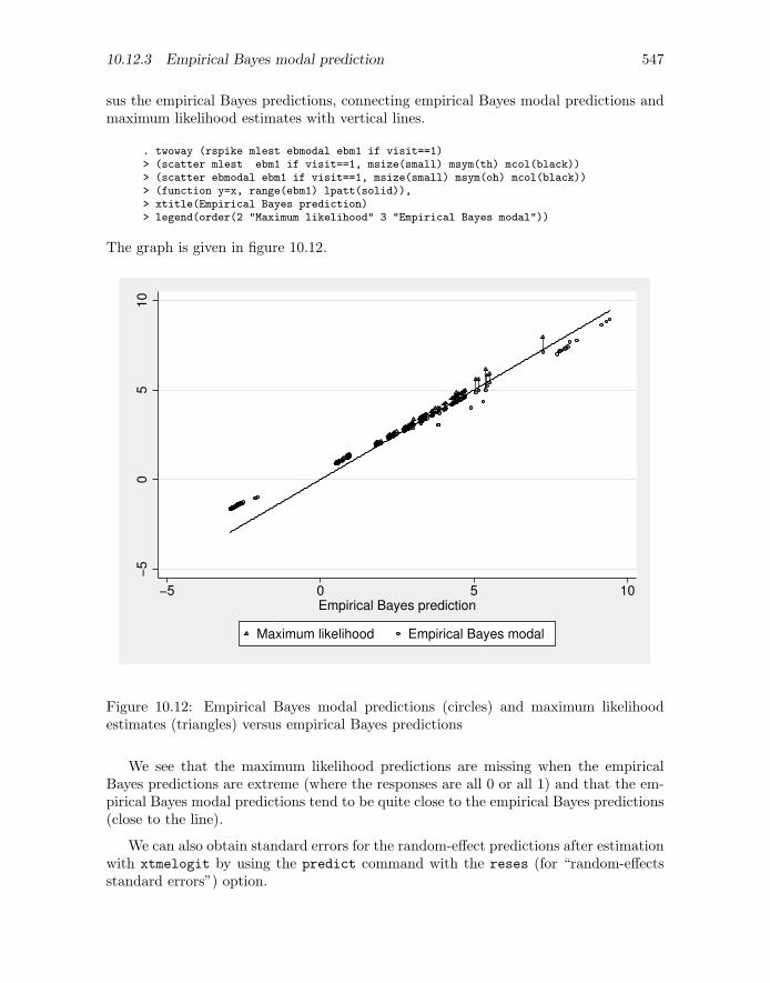
10.12.3 Empirical Bayes modal prediction 547
sus the empirical Bayes predictions, connecting empirical Bayes modal predictions andmaximum likelihood estimates with vertical lines.
. twoway (rspike mlest ebmodal ebm1 if visit==1)> (scatter mlest ebm1 if visit==1, msize(small) msym(th) mcol(black))> (scatter ebmodal ebm1 if visit==1, msize(small) msym(oh) mcol(black))> (function y=x, range(ebm1) lpatt(solid)),> xtitle(Empirical Bayes prediction)> legend(order(2 "Maximum likelihood" 3 "Empirical Bayes modal"))
The graph is given in figure 10.12.
−5
05
10
−5 0 5 10Empirical Bayes prediction
Maximum likelihood Empirical Bayes modal
Figure 10.12: Empirical Bayes modal predictions (circles) and maximum likelihoodestimates (triangles) versus empirical Bayes predictions
We see that the maximum likelihood predictions are missing when the empiricalBayes predictions are extreme (where the responses are all 0 or all 1) and that the em-pirical Bayes modal predictions tend to be quite close to the empirical Bayes predictions(close to the line).
We can also obtain standard errors for the random-effect predictions after estimationwith xtmelogit by using the predict command with the reses (for “random-effectsstandard errors”) option.

548 Chapter 10 Dichotomous or binary responses
. predict se2, reses
These standard errors are the standard deviations of normal densities that approximatethe posterior at the mode. They can be viewed as approximations of the posteriorstandard deviations provided by gllapred. Below we list the predictions and standarderrors produced by gllapred (ebm1 and ebs1) with those produced by predict afterestimation with xtmelogit (ebmodal and se2), together with the number of 0 responses,num0, and the number of 1 responses, num1, for the first 16 patients:
. egen num0 = total(outcome==0), by(patient)
. egen num1 = total(outcome==1), by(patient)
. list patient num0 num1 ebm1 ebmodal ebs1 se2 if visit==1&patient<=12, noobs
patient num0 num1 ebm1 ebmodal ebs1 se2
1 4 3 3.7419957 3.736461 1.0534592 1.0255742 4 2 1.8344596 1.934467 1.0192062 .94234453 6 1 .58899428 .9477552 1.3098199 1.1314514 6 1 .60171957 .9552238 1.3148935 1.1363386 4 3 3.2835777 3.253659 1.0118905 .9709948
7 4 3 3.4032244 3.367345 1.0307951 .99561549 7 0 -2.6807107 -1.399524 2.7073681 2.60882510 7 0 -2.888319 -1.604741 2.6450981 2.50393811 3 4 4.4649443 4.361801 1.0885138 1.07255412 4 3 2.7279723 2.728881 .94173461 .8989795
We see that the predictions and standard errors agree reasonably well (except the ex-treme negative predictions). The standard errors are large when all responses are 0.
10.13 Different kinds of predicted probabilities
10.13.1 Predicted population-averaged or marginal probabilities
At the time of writing this book, population-averaged or marginal probabilities π(xij)can be predicted for random-intercept logistic regression models only by using gllapred
after estimation using gllamm. This is done by evaluating the integral in (10.8) nu-merically for the estimated parameters and values of covariates in the data, that is,evaluating
π(xij) ≡∫
Pr(yij = 1|x2j , x3ij , ζj)φ(ζj ; 0, ψ) dζj
To obtain these predicted marginal probabilities using gllapred, specify the optionsmu (for the mean response, here a probability) and marginal (for integrating over therandom-intercept distribution):
. estimates restore gllamm
. gllapred margprob, mu marginal(mu will be stored in margprob)
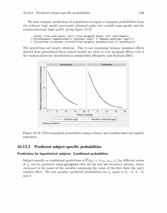
10.13.2 Predicted subject-specific probabilities 549
We now compare predictions of population-averaged or marginal probabilities fromthe ordinary logit model (previously obtained under the variable name prob) and therandom-intercept logit model, giving figure 10.13.
. twoway (line prob month, sort) (line margprob month, sort lpatt(dash)),> by(treatment) legend(order(1 "Ordinary logit" 2 "Random-intercept logit"))> xtitle(Time in months) ytitle(Fitted marginal probabilities of onycholysis)
The predictions are nearly identical. This is not surprising because marginal effectsderived from generalized linear mixed models are close to true marginal effects even ifthe random-intercept distribution is misspecified (Heagerty and Kurland 2001).
0.2
.4
0 5 10 15 20 0 5 10 15 20
Itraconazole Terbinafine
Ordinary logit Random−intercept logit
Fitte
d m
arg
inal pro
babili
ties o
f onycholy
sis
Time in months
Graphs by treatment
Figure 10.13: Fitted marginal probabilities using ordinary and random-intercept logisticregression
10.13.2 Predicted subject-specific probabilities
Predictions for hypothetical subjects: Conditional probabilities
Subject-specific or conditional predictions of Pr(yij = 1|x2j , x3ij , ζj) for different valuesof ζj can be produced using gllapred with the mu and us(varname) options, wherevarname1 is the name of the variable containing the value of the first (here the only)random effect. We now produce predicted probabilities for ζj equal to 0, −4, 4, −2,and 2:

550 Chapter 10 Dichotomous or binary responses
. generate zeta1 = 0
. gllapred condprob0, mu us(zeta)(mu will be stored in condprob0)
. generate lower1 = -4
. gllapred condprobm4, mu us(lower)(mu will be stored in condprobm4)
. generate upper1 = 4
. gllapred condprob4, mu us(upper)(mu will be stored in condprob4)
. replace lower1 = -2(1908 real changes made)
. gllapred condprobm2, mu us(lower)(mu will be stored in condprobm2)
. replace upper1 = 2(1908 real changes made)
. gllapred condprob2, mu us(upper)(mu will be stored in condprob2)
Plotting all of these conditional probabilities together with the observed proportionsand marginal probabilities produces figure 10.14.
. twoway (line prop mn_month, sort)> (line margprob month, sort lpatt(dash))> (line condprob0 month, sort lpatt(shortdash_dot))> (line condprob4 month, sort lpatt(shortdash))> (line condprobm4 month, sort lpatt(shortdash))> (line condprob2 month, sort lpatt(shortdash))> (line condprobm2 month, sort lpatt(shortdash)),> by(treatment)> legend(order(1 "Observed proportion" 2 "Marginal probability"> 3 "Median probability" 4 "Conditional probabilities"))> xtitle(Time in months) ytitle(Probabilities of onycholysis)
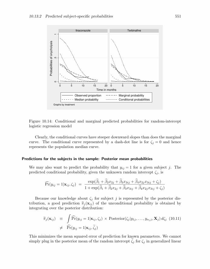
10.13.2 Predicted subject-specific probabilities 551
0.5
1
0 5 10 15 20 0 5 10 15 20
Itraconazole Terbinafine
Observed proportion Marginal probability
Median probability Conditional probabilities
Pro
babili
ties o
f onycholy
sis
Time in months
Graphs by treatment
Figure 10.14: Conditional and marginal predicted probabilities for random-interceptlogistic regression model
Clearly, the conditional curves have steeper downward slopes than does the marginalcurve. The conditional curve represented by a dash-dot line is for ζj = 0 and hencerepresents the population median curve.
Predictions for the subjects in the sample: Posterior mean probabilities
We may also want to predict the probability that yij = 1 for a given subject j. Thepredicted conditional probability, given the unknown random intercept ζj , is
Pr(yij = 1|xij , ζj) =exp(β1 + β2x2j + β3x3ij + β4x2jx3ij + ζj)
1 + exp(β1 + β2x2j + β3x3ij + β4x2jx3ij + ζj)
Because our knowledge about ζj for subject j is represented by the posterior dis-tribution, a good prediction πj(xij) of the unconditional probability is obtained byintegrating over the posterior distribution:
πj(xij) ≡∫
Pr(yij = 1|xij , ζj) × Posterior(ζj |y1j , . . . , ynjj ,Xj) dζj (10.11)
6= Pr(yij = 1|xij , ζj)
This minimizes the mean squared error of prediction for known parameters. We cannotsimply plug in the posterior mean of the random intercept ζj for ζj in generalized linear
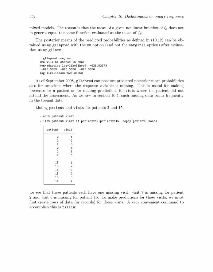
552 Chapter 10 Dichotomous or binary responses
mixed models. The reason is that the mean of a given nonlinear function of ζj does notin general equal the same function evaluated at the mean of ζj .
The posterior means of the predicted probabilities as defined in (10.12) can be ob-tained using gllapred with the mu option (and not the marginal option) after estima-tion using gllamm:
. gllapred cmu, mu(mu will be stored in cmu)Non-adaptive log-likelihood: -625.52573-625.3853 -625.3856 -625.3856
log-likelihood:-625.38558
As of September 2008, gllapred can produce predicted posterior mean probabilitiesalso for occasions where the response variable is missing. This is useful for makingforecasts for a patient or for making predictions for visits where the patient did notattend the assessment. As we saw in section 10.4, such missing data occur frequentlyin the toenail data.
Listing patient and visit for patients 2 and 15,
. sort patient visit
. list patient visit if patient==2|patient==15, sepby(patient) noobs
patient visit
2 12 22 32 42 52 6
15 115 215 315 415 515 7
we see that these patients each have one missing visit: visit 7 is missing for patient2 and visit 6 is missing for patient 15. To make predictions for these visits, we mustfirst create rows of data (or records) for these visits. A very convenient command toaccomplish this is fillin:

10.13.2 Predicted subject-specific probabilities 553
. fillin patient visit
. list patient visit _fillin if patient==2|patient==15, sepby(patient) noobs
patient visit _fillin
2 1 02 2 02 3 02 4 02 5 02 6 02 7 1
15 1 015 2 015 3 015 4 015 5 015 6 115 7 0
fillin finds all values of patient that occur in the data and all values of visit and fillsin all combinations of these values that do not already occur in the data, for example,patient 2 and visit 7. The command creates a new variable, fillin, taking the value1 for filled-in records and 0 for records that existed before. All variables have missingvalues for these new records except patient, visit, and fillin.
Before we can make predictions, we must fill in values for the covariates: treatment,month, and the interaction trt month. Note that, by filling in values for covariates, weare not imputing missing data but just specifying for which covariate values we wouldlike to make predictions.
We start by filling in the appropriate values for treatment, taking into account thattreatment is a time-constant variable.
. egen trt = mean(treatment), by(patient)
. replace treatment = trt if _fillin==1
We proceed by filling in the average time (month) associated with the visit number forthe time-varying variable month by using
. drop mn_month
. egen mn_month = mean(month), by(treatment visit)
. replace month = mn_month if _fillin==1
Finally, we obtain the filled-in version of the interaction variable, trt month, by multi-plying the variables treatment and month that we have constructed:
. replace trt_month = treatment*month
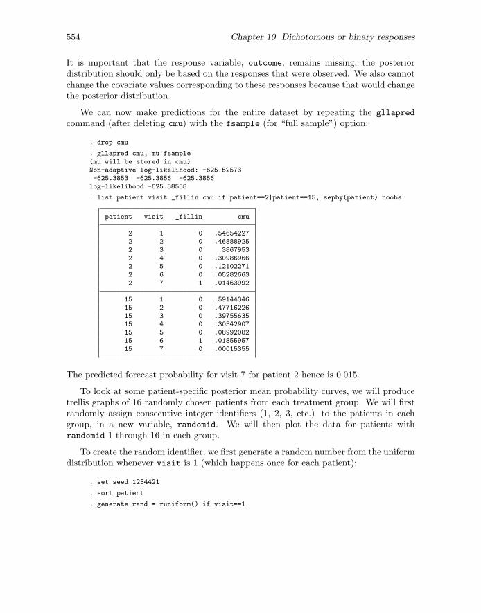
554 Chapter 10 Dichotomous or binary responses
It is important that the response variable, outcome, remains missing; the posteriordistribution should only be based on the responses that were observed. We also cannotchange the covariate values corresponding to these responses because that would changethe posterior distribution.
We can now make predictions for the entire dataset by repeating the gllapred
command (after deleting cmu) with the fsample (for “full sample”) option:
. drop cmu
. gllapred cmu, mu fsample(mu will be stored in cmu)Non-adaptive log-likelihood: -625.52573-625.3853 -625.3856 -625.3856
log-likelihood:-625.38558
. list patient visit _fillin cmu if patient==2|patient==15, sepby(patient) noobs
patient visit _fillin cmu
2 1 0 .546542272 2 0 .468889252 3 0 .38679532 4 0 .309869662 5 0 .121022712 6 0 .052826632 7 1 .01463992
15 1 0 .5914434615 2 0 .4771622615 3 0 .3975563515 4 0 .3054290715 5 0 .0899208215 6 1 .0185595715 7 0 .00015355
The predicted forecast probability for visit 7 for patient 2 hence is 0.015.
To look at some patient-specific posterior mean probability curves, we will producetrellis graphs of 16 randomly chosen patients from each treatment group. We will firstrandomly assign consecutive integer identifiers (1, 2, 3, etc.) to the patients in eachgroup, in a new variable, randomid. We will then plot the data for patients withrandomid 1 through 16 in each group.
To create the random identifier, we first generate a random number from the uniformdistribution whenever visit is 1 (which happens once for each patient):
. set seed 1234421
. sort patient
. generate rand = runiform() if visit==1

10.13.2 Predicted subject-specific probabilities 555
Here use of the set seed and sort commands ensures that you get the same values ofrandomid as we do, because the same “seed” is used for the random-number genera-tor. We now define a variable, randid, that represents the rank order of rand withintreatment groups and is missing when rand is missing:
. by treatment (rand), sort: generate randid = _n if rand<.
randid is the required random identifier, but it is only available when visit is 1 andmissing otherwise. We can fill in the missing values using
. egen randomid = mean(randid), by(patient)
We are now ready to produce the trellis graphs:
. twoway (line cmu month, sort) (scatter cmu month if _fillin==1, mcol(black))> if randomid<=16&treatment==0, by(patient, compact legend(off)> l1title("Posterior mean probabilities"))
and
. twoway (line cmu month, sort) (scatter cmu month if _fillin==1, mcol(black))> if randomid<=16&treatment==1, by(patient, compact legend(off)> l1title("Posterior mean probabilities"))
The graphs are shown in figure 10.15. We see that there is considerable variability inthe probability trajectories of different patients within the same treatment group.
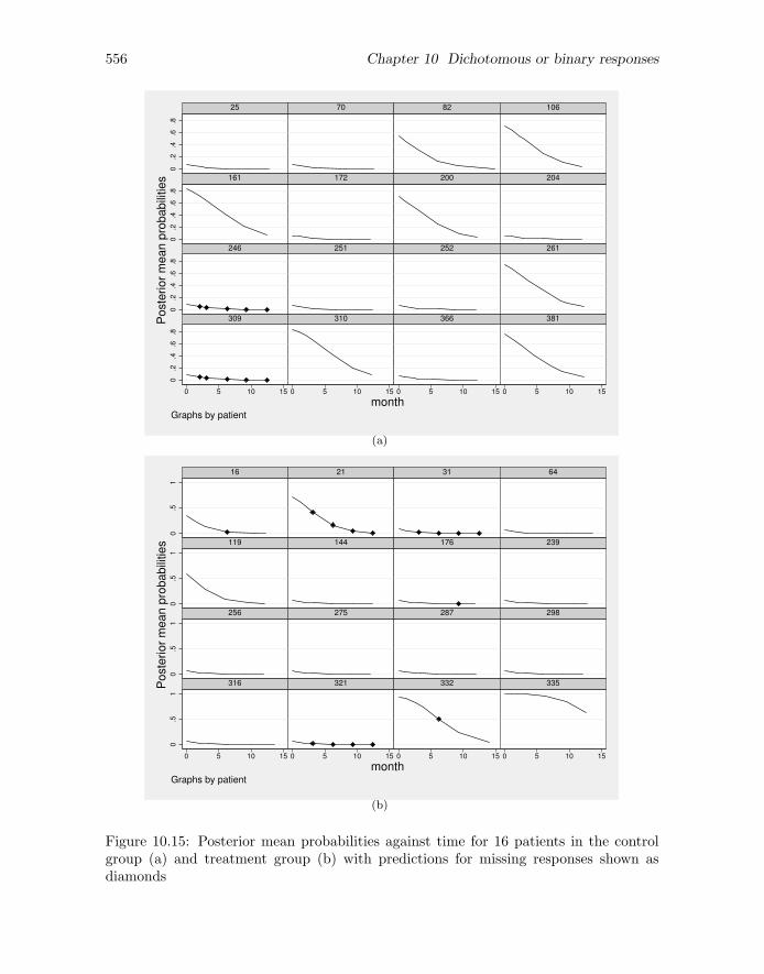
556 Chapter 10 Dichotomous or binary responses
0.2
.4.6
.80
.2.4
.6.8
0.2
.4.6
.80
.2.4
.6.8
0 5 10 15 0 5 10 15 0 5 10 15 0 5 10 15
25 70 82 106
161 172 200 204
246 251 252 261
309 310 366 381Po
ste
rio
r m
ea
n p
rob
ab
ilitie
s
monthGraphs by patient
(a)
0.5
10
.51
0.5
10
.51
0 5 10 15 0 5 10 15 0 5 10 15 0 5 10 15
16 21 31 64
119 144 176 239
256 275 287 298
316 321 332 335Po
ste
rio
r m
ea
n p
rob
ab
ilitie
s
monthGraphs by patient
(b)
Figure 10.15: Posterior mean probabilities against time for 16 patients in the controlgroup (a) and treatment group (b) with predictions for missing responses shown asdiamonds

10.14.1 Conditional logistic regression 557
After estimation with xtmelogit, the predict command with the mu option gives
the posterior mode of the predicted conditional probability Pr(yij |xij , ζj) instead ofthe posterior mean. This is achieved by substituting the posterior mode of ζj into theexpression for the conditional probability. [The mode of a strictly increasing functionof ζj (here an inverse logit), is the same function evaluated at the mode of ζj .]
10.14 Other approaches to clustered dichotomous data
10.14.1 Conditional logistic regression
Instead of using random intercepts for clusters (patients in the toenail application),it would be tempting to use fixed intercepts by including a dummy variable for eachpatient (and omitting the overall intercept). This would be analogous to the fixed-effects estimator of within-patient effects discussed for linear models in section 3.7.2.However, in logistic regression, this approach would lead to inconsistent estimates of thewithin-patient effects unless n is large, due to what is known as the incidental parameterproblem. Roughly speaking, this problem occurs because the number of cluster-specificintercepts (the incidental parameters) increases in tandem with the sample size (numberof clusters), so that the usual asymptotic, or large-sample results, break down. Obvi-ously, we also cannot eliminate the random intercepts in nonlinear models by simplycluster-mean-centering the responses and covariates, as in (3.12).
Instead, we can eliminate the patient-specific intercepts by constructing a likelihoodthat is conditional on the number of responses that take the value 1 (a sufficient statisticfor the patient-specific intercept). This approach is demonstrated in display 12.2 inthe chapter on nominal responses. In the linear case, assuming normality, ordinaryleast-squares estimation of the cluster-mean-centered model is equivalent to conditionalmaximum likelihood estimation. In logistic regression, conditional maximum likelihoodestimation is more involved and is known as conditional logistic regression. Importantly,this method estimates conditional or subject-specific effects. When using conditionallogistic regression, we can only estimate the effects of within-patient or time-varyingcovariates. Patient-specific covariates, such as treatment, cannot be included. However,interactions between patient-specific and time-varying variables, such as treatment bymonth, can be estimated.
Conditional logistic regression can be performed using Stata’s xtlogit commandwith the fe option or using the clogit command (with the or option to obtain oddsratios):
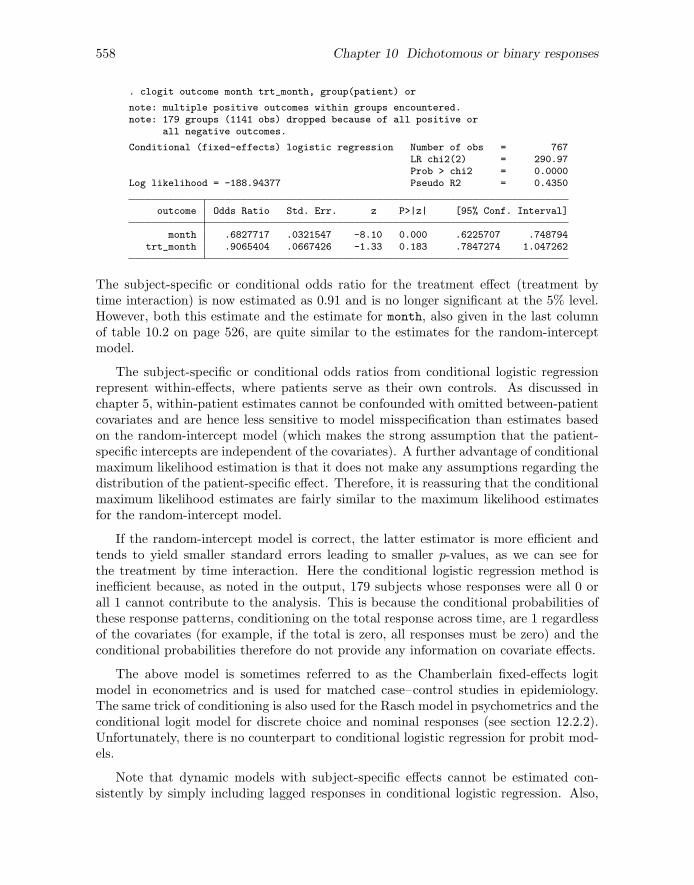
558 Chapter 10 Dichotomous or binary responses
. clogit outcome month trt_month, group(patient) or
note: multiple positive outcomes within groups encountered.note: 179 groups (1141 obs) dropped because of all positive or
all negative outcomes.
Conditional (fixed-effects) logistic regression Number of obs = 767LR chi2(2) = 290.97Prob > chi2 = 0.0000
Log likelihood = -188.94377 Pseudo R2 = 0.4350
outcome Odds Ratio Std. Err. z P>|z| [95% Conf. Interval]
month .6827717 .0321547 -8.10 0.000 .6225707 .748794trt_month .9065404 .0667426 -1.33 0.183 .7847274 1.047262
The subject-specific or conditional odds ratio for the treatment effect (treatment bytime interaction) is now estimated as 0.91 and is no longer significant at the 5% level.However, both this estimate and the estimate for month, also given in the last columnof table 10.2 on page 526, are quite similar to the estimates for the random-interceptmodel.
The subject-specific or conditional odds ratios from conditional logistic regressionrepresent within-effects, where patients serve as their own controls. As discussed inchapter 5, within-patient estimates cannot be confounded with omitted between-patientcovariates and are hence less sensitive to model misspecification than estimates basedon the random-intercept model (which makes the strong assumption that the patient-specific intercepts are independent of the covariates). A further advantage of conditionalmaximum likelihood estimation is that it does not make any assumptions regarding thedistribution of the patient-specific effect. Therefore, it is reassuring that the conditionalmaximum likelihood estimates are fairly similar to the maximum likelihood estimatesfor the random-intercept model.
If the random-intercept model is correct, the latter estimator is more efficient andtends to yield smaller standard errors leading to smaller p-values, as we can see forthe treatment by time interaction. Here the conditional logistic regression method isinefficient because, as noted in the output, 179 subjects whose responses were all 0 orall 1 cannot contribute to the analysis. This is because the conditional probabilities ofthese response patterns, conditioning on the total response across time, are 1 regardlessof the covariates (for example, if the total is zero, all responses must be zero) and theconditional probabilities therefore do not provide any information on covariate effects.
The above model is sometimes referred to as the Chamberlain fixed-effects logitmodel in econometrics and is used for matched case–control studies in epidemiology.The same trick of conditioning is also used for the Rasch model in psychometrics and theconditional logit model for discrete choice and nominal responses (see section 12.2.2).Unfortunately, there is no counterpart to conditional logistic regression for probit mod-els.
Note that dynamic models with subject-specific effects cannot be estimated con-sistently by simply including lagged responses in conditional logistic regression. Also,
10.14.2 Generalized estimating equations (GEE) 559
subject-specific predictions are not possible in conditional logistic regression because noinferences are made regarding the subject-specific intercepts.
10.14.2 Generalized estimating equations (GEE)
Generalized estimating equations (GEE), first introduced in section 6.6, can be used toestimate marginal or population-averaged effects. Dependence among the responses ofunits in a given cluster is taken into account but treated as a nuisance, whereas thisdependence is of central interest in multilevel modeling.
The basic idea of GEE is that an algorithm, known as reweighted iterated leastsquares, for maximum likelihood estimation of single-level generalized linear modelsrequires only the mean structure (expectation of the response variable as a function ofthe covariates) and the variance function. The algorithm iterates between linearizingthe model given current parameter estimates and then updating the parameters usingweighted least squares, with weights determined by the variance function. In GEE, thisiterative algorithm is extended to two-level data by assuming a within-cluster correlationstructure, in addition to the mean structure and variance function, so that the weightedleast-squares step becomes a generalized least-squares step (see section 3.10.1), andanother step is required for updating the correlation matrix. GEE can be viewed asa special case of generalized methods of moments (GMM) estimation (implemented inStata’s gmm command).
In addition to specifying a model for the marginal relationship between the responsevariable and covariates, it is necessary to choose a structure for the correlations amongthe observed responses (conditional on covariates). The variance function follows fromthe Bernoulli distribution. The most common correlation structures are (see section 6.6for some other correlation structures):
• Independence:Same as ordinary logistic regression
• Exchangeable:Same correlation for all pairs of units
• Autoregressive lag-1 [AR(1)]:Correlation declines exponentially with the time lag—only makes sense for longi-tudinal data and assumes constant time intervals between occasions (but allowsgaps due to missing data).
• Unstructured:A different correlation for each pair of responses—only makes sense if units are notexchangeable within clusters, in the sense that the labels i attached to the unitsmean the same thing across clusters. For instance, it is meaningful in longitudinaldata where units are occasions and the first occasion means the same thing acrossindividuals, but not in data on students nested in schools where the numberingof students is arbitrary. In addition, each pair of unit labels i and i′ must occursufficiently often across clusters to estimate the pairwise correlations. Finally, the
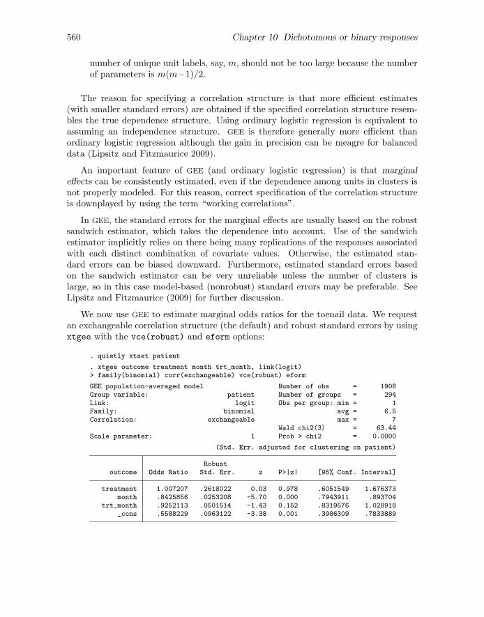
560 Chapter 10 Dichotomous or binary responses
number of unique unit labels, say, m, should not be too large because the numberof parameters is m(m−1)/2.
The reason for specifying a correlation structure is that more efficient estimates(with smaller standard errors) are obtained if the specified correlation structure resem-bles the true dependence structure. Using ordinary logistic regression is equivalent toassuming an independence structure. GEE is therefore generally more efficient thanordinary logistic regression although the gain in precision can be meagre for balanceddata (Lipsitz and Fitzmaurice 2009).
An important feature of GEE (and ordinary logistic regression) is that marginaleffects can be consistently estimated, even if the dependence among units in clusters isnot properly modeled. For this reason, correct specification of the correlation structureis downplayed by using the term “working correlations”.
In GEE, the standard errors for the marginal effects are usually based on the robustsandwich estimator, which takes the dependence into account. Use of the sandwichestimator implicitly relies on there being many replications of the responses associatedwith each distinct combination of covariate values. Otherwise, the estimated stan-dard errors can be biased downward. Furthermore, estimated standard errors basedon the sandwich estimator can be very unreliable unless the number of clusters islarge, so in this case model-based (nonrobust) standard errors may be preferable. SeeLipsitz and Fitzmaurice (2009) for further discussion.
We now use GEE to estimate marginal odds ratios for the toenail data. We requestan exchangeable correlation structure (the default) and robust standard errors by usingxtgee with the vce(robust) and eform options:
. quietly xtset patient
. xtgee outcome treatment month trt_month, link(logit)> family(binomial) corr(exchangeable) vce(robust) eform
GEE population-averaged model Number of obs = 1908Group variable: patient Number of groups = 294Link: logit Obs per group: min = 1Family: binomial avg = 6.5Correlation: exchangeable max = 7
Wald chi2(3) = 63.44Scale parameter: 1 Prob > chi2 = 0.0000
(Std. Err. adjusted for clustering on patient)
Robustoutcome Odds Ratio Std. Err. z P>|z| [95% Conf. Interval]
treatment 1.007207 .2618022 0.03 0.978 .6051549 1.676373month .8425856 .0253208 -5.70 0.000 .7943911 .893704
trt_month .9252113 .0501514 -1.43 0.152 .8319576 1.028918_cons .5588229 .0963122 -3.38 0.001 .3986309 .7833889
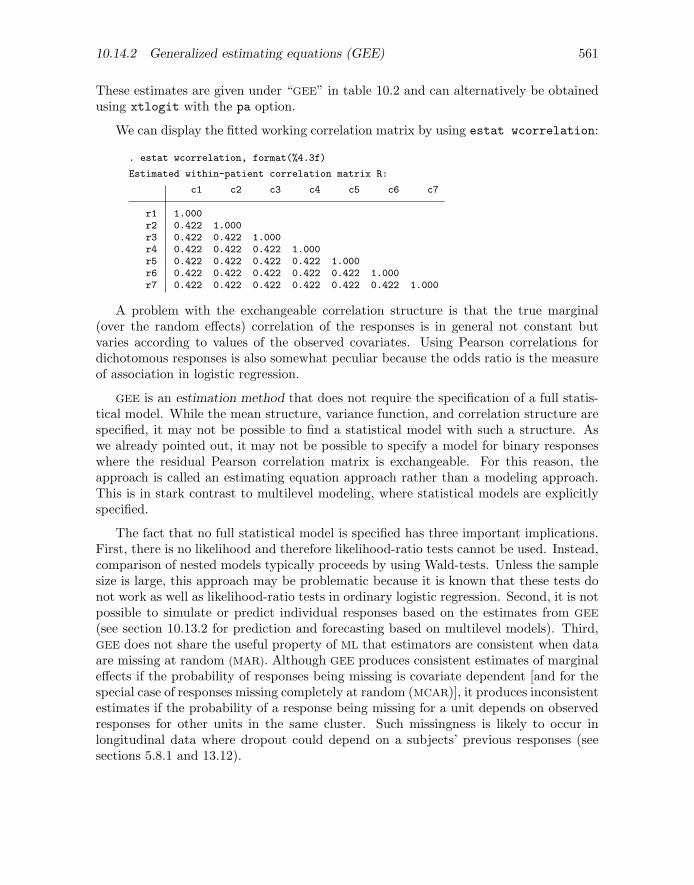
10.14.2 Generalized estimating equations (GEE) 561
These estimates are given under “GEE” in table 10.2 and can alternatively be obtainedusing xtlogit with the pa option.
We can display the fitted working correlation matrix by using estat wcorrelation:
. estat wcorrelation, format(%4.3f)
Estimated within-patient correlation matrix R:
c1 c2 c3 c4 c5 c6 c7
r1 1.000r2 0.422 1.000r3 0.422 0.422 1.000r4 0.422 0.422 0.422 1.000r5 0.422 0.422 0.422 0.422 1.000r6 0.422 0.422 0.422 0.422 0.422 1.000r7 0.422 0.422 0.422 0.422 0.422 0.422 1.000
A problem with the exchangeable correlation structure is that the true marginal(over the random effects) correlation of the responses is in general not constant butvaries according to values of the observed covariates. Using Pearson correlations fordichotomous responses is also somewhat peculiar because the odds ratio is the measureof association in logistic regression.
GEE is an estimation method that does not require the specification of a full statis-tical model. While the mean structure, variance function, and correlation structure arespecified, it may not be possible to find a statistical model with such a structure. Aswe already pointed out, it may not be possible to specify a model for binary responseswhere the residual Pearson correlation matrix is exchangeable. For this reason, theapproach is called an estimating equation approach rather than a modeling approach.This is in stark contrast to multilevel modeling, where statistical models are explicitlyspecified.
The fact that no full statistical model is specified has three important implications.First, there is no likelihood and therefore likelihood-ratio tests cannot be used. Instead,comparison of nested models typically proceeds by using Wald-tests. Unless the samplesize is large, this approach may be problematic because it is known that these tests donot work as well as likelihood-ratio tests in ordinary logistic regression. Second, it is notpossible to simulate or predict individual responses based on the estimates from GEE
(see section 10.13.2 for prediction and forecasting based on multilevel models). Third,GEE does not share the useful property of ML that estimators are consistent when dataare missing at random (MAR). Although GEE produces consistent estimates of marginaleffects if the probability of responses being missing is covariate dependent [and for thespecial case of responses missing completely at random (MCAR)], it produces inconsistentestimates if the probability of a response being missing for a unit depends on observedresponses for other units in the same cluster. Such missingness is likely to occur inlongitudinal data where dropout could depend on a subjects’ previous responses (seesections 5.8.1 and 13.12).
562 Chapter 10 Dichotomous or binary responses
10.15 Summary and further reading
We have described various approaches to modeling clustered dichotomous data, focusingon random-intercept models for longitudinal data. Alternatives to multilevel modeling,such as conditional maximum likelihood estimation and generalized estimating equa-tions, have also been briefly discussed. The important distinction between conditionalor subject-specific effects and marginal or population-averaged effects has been empha-sized.
We have described adaptive quadrature for maximum likelihood estimation andpointed out that you need to make sure that a sufficient number of quadrature pointshave been used for a given model and application. We have demonstrated the use of avariety of predictions, either cluster-specific predictions, based on empirical Bayes, orpopulation-averaged predictions. Keep in mind that consistent estimation in logisticregression models with random effects in principle requires a completely correct modelspecification. Diagnostics for generalized linear mixed models are still being developed.
We did not cover random-coefficient models for binary responses in this chapterbut have included two exercises (10.3 and 10.8), with solutions provided, involvingthese models. The issues discussed in chapter 4 regarding linear models with randomcoefficients are also relevant for other generalized linear mixed models. The syntaxfor random-coefficient logistic models is analogous to the syntax for linear random-coefficient models except that xtmixed is replaced with xtmelogit and gllamm isused with a different link function and distribution (the syntax for linear random-coefficient models in gllamm can be found in the gllamm companion). Three-levelrandom-coefficient logistic models for binary responses are discussed in chapter 16. Inchapter 11, gllamm will be used to fit random-coefficient ordinal logistic regression mod-els; see section 11.7.2.
Dynamic or lagged-response models for binary responses have not been discussed.The reason is that such models, sometimes called transition models in this context, cansuffer from similar kinds of endogeneity problems as those discussed for dynamic modelswith random intercepts in chapter 5 of volume I. However, these problems are not asstraightforward to address for binary responses (but see Wooldridge [2005]).
We have discussed the most common link functions for dichotomous responses,namely, logit and probit links. A third link that is sometimes used is the comple-mentary log-log link, which is introduced in section 14.6. Dichotomous responses aresometimes aggregated into counts, giving the number of successes yi in ni trials for uniti. In this situation, it is usually assumed that yi has a binomial(ni,πi) distribution.xtmelogit can then be used as for dichotomous responses but with the binomial()
option to specify the variable containing the values ni. Similarly, gllamm can be usedwith the binomial distribution and any of the link functions together with the denom()
option to specify the variable containing ni.

10.16 Exercises 563
Good introductions to single-level logistic regression include Collett (2003a), Long(1997), and Hosmer and Lemeshow (2000). Logistic and other types of regression usingStata are discussed by Long and Freese (2006), primarily with examples from socialscience, and by Vittinghoff et al. (2005), with examples from medicine.
Generalized linear mixed models are described in the books by McCulloch, Searle,and Neuhaus (2008), Skrondal and Rabe-Hesketh (2004), Molenberghs and Verbeke(2005), and Hedeker and Gibbons (2006). See also Goldstein (2011), Raudenbush andBryk (2002), and volume 3 of the anthology by Skrondal and Rabe-Hesketh (2010). Sev-eral examples with dichotomous responses are discussed in Skrondal and Rabe-Hesketh(2004, chap. 9). Guo and Zhao (2000) is a good introductory paper on multilevel mod-eling of binary data with applications in social science. We also recommend the bookchapter by Rabe-Hesketh and Skrondal (2009), the article by Agresti et al. (2000), andthe encyclopedia entry by Hedeker (2005) for overviews of generalized linear mixed mod-els. Detailed accounts of generalized estimating equations are given in Hardin and Hilbe(2003), Diggle et al. (2002), and Lipsitz and Fitzmaurice (2009).
Exercises 10.1, 10.2, 10.3, and 10.6 are on longitudinal or panel data. There are alsoexercises on cross-sectional datasets on students nested in schools (10.7 and 10.8), cowsnested in herds (10.5), questions nested in respondents (10.4) and wine bottles nestedin judges (10.9). Exercise 10.2 involves GEE, whereas exercises 10.4 and 10.6 involveconditional logistic regression. The latter exercise also asks you to perform a Hausmantest. Exercises 10.3 and 10.8 consider random-coefficient models for dichotomous re-sponses (solutions are provided for both exercises). Exercise 10.4 introduces the idea ofitem-response theory, and exercise 10.8 shows how gllamm can be used to fit multilevelmodels with survey weights.
10.16 Exercises
10.1 Toenail data
1. Fit the probit version of the random-intercept model in (10.6) with gllamm.How many quadrature points appear to be needed using adaptive quadrature?
2. Estimate the residual intraclass correlation for the latent responses.
3. Obtain empirical Bayes predictions using both the random-intercept logitand probit models and estimate the approximate constant of proportionalitybetween these.
4. q By considering the residual standard deviations of the latent responsefor the logit and probit models, work out what you think the constant ofproportionality should be for the logit- and probit-based empirical Bayespredictions. How does this compare with the constant estimated in step 3?
564 Chapter 10 Dichotomous or binary responses
10.2 Ohio wheeze data
In this exercise, we use data from the Six Cities Study (Ware et al. 1984), previ-ously analyzed by Fitzmaurice (1998), among others. The dataset includes 537children from Steubenville, Ohio, who were examined annually four times from age7 to age 10 to ascertain their wheezing status. The smoking status of the motherwas also determined at the beginning of the study to investigate whether maternalsmoking increases the risk of wheezing in children. The mother’s smoking statusis treated as time constant, although it may have changed for some mothers overtime.
The dataset wheeze.dta has the following variables:
• id: child identifier (j)
• age: number of years since ninth birthday (x2ij)
• smoking: mother smokes regularly (1: yes; 0: no) (x3j)
• y: wheeze status (1: yes; 0: no) (yij)
1. Fit the following transition model considered by Fitzmaurice (1998):
logit{Pr(yij =1|xij , yi−1,j)} = β1 + β2x2ij + β3x3j + γyi−1,j , i = 2, 3, 4
where x2ij is age and x3j is smoking. (The lagged responses can be obtainedusing by id (age), sort: generate lag = y[ n-1]. Alternatively, usethe time-series operator L.; see table 5.3 on page 275.)
2. Fit the following random-intercept model considered by Fitzmaurice (1998):
logit{Pr(yij =1|xij , ζj)} = β1 + β2x2ij + β3x3j + ζj , i = 1, 2, 3, 4
It is assumed that ζj ∼ N(0, ψ), and that ζj is independent across childrenand independent of xij .
3. Use GEE to fit the marginal model
logit{Pr(yij =1|xij)} = β1 + β2x2ij + β3x3j , i = 1, 2, 3, 4
specifying an unstructured correlation matrix (xtset the data using xtset
id age). Try some other correlation structures and compare the fit (usingestat wcorrelation) to the unstructured version.
4. Interpret the estimated effects of mother’s smoking status for the models insteps 1, 2, and 3.
10.3 Vaginal-bleeding dataSolutions
Fitzmaurice, Laird, and Ware (2011) analyzed data from a trial reported byMachin et al. (1988). Women were randomized to receive an injection of either100 mg or 150 mg of the long-lasting injectable contraception depot medroxypro-gesterone acetate (DMPA) at the start of the trial and at three successive 90-day

10.16 Exercises 565
intervals. In addition, the women were followed up 90 days after the final injection.Throughout the study, each woman completed a menstrual diary that recordedany vaginal bleeding pattern disturbances. The diary data were used to determinewhether a woman experienced amenorrhea, defined as the absence of menstrualbleeding for at least 80 consecutive days.
The response variable for each of the four 90-day intervals is whether the womanexperienced amenorrhea during the interval. Data are available on 1,151 womenfor the first interval, but there was considerable dropout after that.
The dataset amenorrhea.dta has the following variables:
• dose: high dose (1: yes; 0: no)
• y1–y4: responses for time intervals 1–4 (1: amenorrhea; 0: no amenorrhea)
• wt2: number of women with the same dose level and response pattern
1. Produce an identifier variable for women, and reshape the data to long form,stacking the responses y1–y4 into one variable and creating a new variable,occasion, taking the values 1–4 for each woman.
2. Fit the following model considered by Fitzmaurice, Laird, and Ware (2011):
logit{Pr(yij = 1|xj , tij , ζj)} = β1 + β2tij + β3t2ij + β4xjtij + β5xjt
2ij + ζj
where tij = 1, 2, 3, 4 is the time interval and xj is dose. It is assumed thatζj ∼ N(0, ψ), and that ζj is independent across women and independent ofxj and tij . Use gllamm with the weight(wt) option to specify that wt2 arelevel-2 weights.
3. Write down the above model but with a random slope of tij , and fit themodel. (See section 11.7.2 for an example of a random-coefficient model fitin gllamm.)
4. Interpret the estimated coefficients.
5. Plot marginal predicted probabilities as a function of time, separately forwomen in the two treatment groups.
10.4 Verbal-aggression data
De Boeck and Wilson (2004) discuss a dataset from Vansteelandt (2000) where316 participants were asked to imagine the following four frustrating situationswhere either another or oneself is to blame:
1. Bus: A bus fails to stop for me (another to blame)
2. Train: I miss a train because a clerk gave me faulty information (another toblame)
3. Store: The grocery store closes just as I am about to enter (self to blame)
4. Operator: The operator disconnects me when I have used up my last 10 centsfor a call (self to blame)

566 Chapter 10 Dichotomous or binary responses
For each situation, the participant was asked if it was true (yes, perhaps, or no)that
1. I would (want to) curse
2. I would (want to) scold
3. I would (want to) shout
For each of the three behaviors above, the words “want to” were both includedand omitted, yielding six statements with a 3 × 2 factorial design (3 behaviors in2 modes) combined with the four situations. Thus there were 24 items in total.
The dataset aggression.dta contains the following variables:
• person: subject identifier
• item: item (or question) identifier
• description: item description(situation: bus/train/store/operator; behavior: curse/scold/shout; mode:do/want)
• i1–i24: dummy variables for the items, for example, i5 equals 1 when item
equals 5 and 0 otherwise
• y: ordinal response (0: no; 1: perhaps; 2: yes)
• Person characteristics:
– anger: trait anger score (STAXI, Spielberger [1988]) (w1j)– gender: dummy variable for being male (1: male; 0: female) (w2j)
• Item characteristics:
– do want: dummy variable for mode being “do” (that is, omitting words“want to”) versus “want” (x2ij)
– other self: dummy variable for others to blame versus self to blame(x3ij)
– blame: variable equal to 0.5 for blaming behaviors curse and scold and−1 for shout (x4ij)
– express: variable equal to 0.5 for expressive behaviors curse and shoutand −1 for scold (x5ij)
1. Recode the ordinal response variable y so that either a “2” or a “1” for theoriginal variable becomes a “1” for the recoded variable.
2. De Boeck and Wilson (2004, sec. 2.5) consider the following “explanatoryitem-response model” for the dichotomous response
logit{Pr(yij =1|xij , ζj)} = β1 + β2x2ij + β3x3ij + β4x4ij + β5x5ij + ζj
where ζj ∼ N(0, ψ) can be interpreted as the latent trait “verbal aggressive-ness”. Fit this model using xtlogit, and interpret the estimated coefficients.In De Boeck and Wilson (2004), the first five terms have minus signs, so theirestimated coefficients have the opposite sign.

10.16 Exercises 567
3. De Boeck and Wilson (2004, sec. 2.6) extend the above model by includinga latent regression, allowing verbal aggressiveness (now denoted ηj insteadof ζj) to depend on the person characteristics w1j and w2j :
logit{Pr(yij =1|xij , ηj)} = β1 + β2x2ij + β3x3ij + β4x4ij + β5x5ij + ηj
ηj = γ1w1j + γ2w2j + ζj
Substitute the level-2 model for ηj into the level-1 model for the item re-sponses, and fit the model using xtlogit.
4. Use xtlogit to fit the “descriptive item-response model”, usually called aone-parameter logistic item response (IRT) model or Rasch model, consideredby De Boeck and Wilson (2004, sec. 2.3):
logit{Pr(yij =1|d1i, . . . , d24,i, ζj)} =24∑
m=1
βmdmi + ζj
where dmi is a dummy variable for item i, with dmi = 1 if m = i and 0otherwise. In De Boeck and Wilson (2004), the first term has a minus sign,so their βm coefficients have the opposite sign; see also their page 53.
5. The model above is known as a one-parameter item-response model becausethere is one parameter βm for each item. The negative of these item-specificparameters −βm can be interpreted as “difficulties”; the larger −βm, thelarger the latent trait (here verbal aggressiveness, but often ability) has tobe to yield a given probability (for example, 0.5) of a 1 response.
Sort the items in increasing order of the estimated difficulties. For the leastand most difficult items, look up the variable description, and discusswhether it makes sense that these items are particularly easy and hard toendorse (requiring little and a lot of verbal aggressiveness), respectively.
6. Replace the random intercepts ζj with fixed parameters αj . Set the difficultyof the first item to zero for identification and fit the model by conditionalmaximum likelihood. Verify that differences between estimated difficultiesfor the items are similar as in step 4.
7. q Fit the model in step 4 using gllamm or xtmelogit (this will take longerthan xtlogit) and obtain empirical Bayes (also called EAP) or empiricalBayes modal (also called MAP) predictions (depending on whether you fitthe model in gllamm or xtmelogit, respectively) and ML estimates of the la-tent trait. Also obtain standard errors (for ML, this means saving se[ cons]
in addition to b[ cons] by adding mlse = se[ cons] in the statsby com-mand). Does there appear to be much shrinkage? Calculate the total score(sum of item responses) for each person and plot curves of the different kindsof standard errors with total score on the x axis. Comment on what you find.
See also exercise 11.2 for further analyses of these data.
568 Chapter 10 Dichotomous or binary responses
10.5 Dairy-cow data
Dohoo et al. (2001) and Dohoo, Martin, and Stryhn (2010) analyzed data on dairycows from Reunion Island. One outcome considered was the “risk” of conceptionat the first insemination attempt (first service) since the previous calving. Thisoutcome was available for several lactations (calvings) per cow.
The variables in the dataset dairy.dta used here are
• cow: cow identifier
• herd: herd identifier
• region: geographic region
• fscr: first service conception risk (dummy variable for cow becoming preg-nant)
• lncfs: log of time interval (in log days) between calving and first service(insemination attempt)
• ai: dummy variable for artificial insemination being used (versus natural) atfirst service
• heifer: dummy variable for being a young cow that has calved only once
1. Fit a two-level random-intercept logistic regression model for the responsevariable fscr, an indicator for conception at the first insemination attempt(first service). Include a random intercept for cow and the covariates lncfs,ai, and heifer. (Use either xtlogit, xtmelogit, or gllamm.)
2. Obtain estimated odds ratios with 95% confidence intervals for the covariatesand interpret them.
3. Obtain the estimated residual intraclass correlation between the latent re-sponses for two observations on the same cow. Is there much variability inthe cows’ fertility?
4. Obtain the estimated median odds ratio for two randomly chosen cows withthe same covariates, comparing the cow that has the larger random interceptwith the cow that has the smaller random intercept.
See also exercises 8.8 and 16.1.
10.6 Union membership data
Vella and Verbeek (1998) analyzed panel data on 545 young males taken from theU.S. National Longitudinal Survey (Youth Sample) for the period 1980–1987. Inthis exercise, we will focus on modeling whether the men were members of unionsor not.
The dataset wagepan.dta was provided by Wooldridge (2010) and was previouslyused in exercise 3.6 and Introduction to models for longitudinal and panel data(part III). The subset of variables considered here is

10.16 Exercises 569
• nr: person identifier (j)
• year: 1980–1987 (i)
• union: dummy variable for being a member of a union (that is, wage beingset in collective bargaining agreement) (yij)
• educ: years of schooling (x2j)
• black: dummy variable for being black (x3j)
• hisp: dummy variable for being Hispanic (x4j)
• exper: labor market experience, defined as age−6−educ (x5ij)
• married: dummy variable for being married (x6ij)
• rur: dummy variable for living in a rural area (x7ij)
• nrtheast: dummy variable for living in Northeast (x8ij)
• nrthcen: dummy variable for living in Northern Central (x9ij)
• south: dummy variable for living in South (x10,ij)
You can use the describe command to get a description of the other variables inthe file.
1. Use maximum likelihood to fit the random-intercept logistic regression model
logit{Pr(yij = 1|xij , ζj)} = β1 + β2x2j + · · · + β11x10,ij + ζj
where ζj ∼ N(0, ψ), and ζj is assumed to be independent across persons andindependent of xij . Use xtlogit because it is considerably faster than theother commands here.
2. Interpret the estimated effects of the covariates from step 1 in terms of oddsratios, and report the estimated residual intraclass correlation of the latentresponses.
3. Fit the marginal model
logit{Pr(yij = 1|xij)} = β1 + β2x2j + · · · + β11x10,ij
using GEE with an exchangeable working correlation structure.
4. Interpret the estimated effects of the covariates from step 3 in terms of oddsratios, and compare these estimates with those from step 1. Why are theestimates different?
5. Explore the within and between variability of the response variable and co-variates listed above. For which of the covariates is it impossible to estimatean effect using a fixed-effects approach? Are there any covariates whose ef-fects you would expect to be imprecisely estimated when using a fixed-effectsapproach?
6. Use conditional maximum likelihood to fit the fixed-intercept logistic regres-sion model

570 Chapter 10 Dichotomous or binary responses
logit{Pr(yij = 1|xij)} = β1 + β2x2j + · · · + β11x10,ij + αj
where the αj are unknown person-specific parameters.
7. Interpret the estimated effects of the covariates from step 6 in terms of oddsratios, and compare these estimates with those from step 1. Why are theestimates different?
8. Perform a Hausman test to assess the validity of the random-intercept model.What do you conclude?
9. Fit the probit versions of the random-intercept model from step 1 usingxtprobit. Which type of model do you find easiest to interpret?
10.7 School retention in Thailand data
A national survey of primary education was conducted in Thailand in 1988. Thedata were previously analyzed by Raudenbush and Bhumirat (1992) and are dis-tributed with the HLM software (Raudenbush et al. 2004). Here we will modelthe probability that a child repeats a grade any time during primary school.
The dataset thailand.dta has the following variables:
• rep: dummy variable for child having repeated a grade during primary school(yij)
• schoolid: school identifier (j)
• pped: dummy variable for child having preprimary experience (x2ij)
• male: dummy variable for child being male (x3ij)
• mses: school mean socioeconomic status (SES) (x4j)
• wt1: number of children in the school having a given set of values of rep,pped, and male (level-1 frequency weights)
1. Fit the model
logit{Pr(yij = 1|xij , ζj)} = β1 + β2x2ij + β3x3ij + β4x4j + ζj
where ζj ∼ N(0, ψ), and ζj is independent across schools and independent ofthe covariates xij . Use gllamm with the weight(wt) option to specify thateach row in the data represents wt1 children (level-1 units).
2. Obtain and interpret the estimated odds ratios and the estimated residualintraschool correlation of the latent responses.
3. Use gllapred to obtain empirical Bayes predictions of the probability ofrepeating a grade. These probabilities will be specific to the schools, as wellas dependent on the student-level predictors.
a. List the values of male, pped, rep, wt1, and the predicted probabilitiesfor the school with schoolid equal to 10104. Explain why the predictedprobabilities are greater than 0 although none of the children in thesample from that school have been retained. For comparison, list thesame variables for the school with schoolid equal to 10105.

10.16 Exercises 571
b. Produce box plots of the predicted probabilities for each school by male
and pped (for instance, using by(male) and over(pped)). To ensure thateach school contributes no more than four probabilities to the graph (onefor each combination of the student-level covariates), use only responseswhere rep is 0 (that is, if rep==0). Do the schools appear to be variablein their retention probabilities?
10.8 PISA dataSolutions
Here we consider data from the 2000 Program for International Student Assess-ment (PISA) conducted by the Organization for Economic Cooperation and De-velopment (OECD 2000) that are made available with permission from MariannLemke. The survey assessed educational attainment of 15-year-olds in 43 coun-tries in various areas, with an emphasis on reading. Following Rabe-Heskethand Skrondal (2006), we will analyze reading proficiency, treated as dichotomous(1: proficient; 0: not proficient), for the U.S. sample.
The variables in the dataset pisaUSA2000.dta are
• id school: school identifier
• pass read: dummy variable for being proficient in reading
• female: dummy variable for student being female
• isei: international socioeconomic index
• high school: dummy variable for highest education level by either parentbeing high school
• college: dummy variable for highest education level by either parent beingcollege
• test lang: dummy variable for test language (English) being spoken at home
• one for: dummy variable for one parent being foreign born
• both for: dummy variable for both parents being foreign born
• w fstuwt: student-level or level-1 survey weights
• wnrschbq: school-level or level-2 survey weights
1. Fit a logistic regression model with pass read as the response variable andthe variables female to both for above as covariates and with a randomintercept for schools using gllamm. (Use the default eight quadrature points.)
2. Fit the model from step 1 with the school mean of isei as an additionalcovariate. (Use the estimates from step 1 as starting values.)
3. Interpret the estimated coefficients of isei and school mean isei and com-ment on the change in the other parameter estimates due to adding schoolmean isei.
4. From the estimates in step 2, obtain an estimate of the between-school effectof socioeconomic status.
5. Obtain robust standard errors using the command gllamm, robust, andcompare them with the model-based standard errors.

572 Chapter 10 Dichotomous or binary responses
6. Add a random coefficient of isei, and compare the random-intercept andrandom-coefficient models using a likelihood-ratio test. Use the estimatesfrom step 2 (or step 5) as starting values, adding zeros for the two additionalparameters as shown in section 11.7.2.
7. q In this survey, schools were sampled with unequal probabilities, πj , andgiven that a school was sampled, students were sampled from the schoolwith unequal probabilities πi|j . The reciprocals of these probabilities aregiven as school- and student-level survey weights, wnrschbg (wj = 1/πj) andw fstuwt (wi|j = 1/πi|j), respectively. As discussed in Rabe-Hesketh andSkrondal (2006), incorporating survey weights in multilevel models using aso-called pseudolikelihood approach can lead to biased estimates, particularlyif the level-1 weights wi|j are different from 1 and if the cluster sizes are small.Neither of these issues arises here, so implement pseudomaximum likelihoodestimation as follows:
a. Rescale the student-level weights by dividing them by their cluster means[this is scaling method 2 in Rabe-Hesketh and Skrondal (2006)].
b. Rename the level-2 weights and rescaled level-1 weights to wt2 and wt1,respectively.
c. Run the gllamm command from step 2 above with the additional optionpweight(wt). (Only the stub of the weight variables is specified; gllammwill look for the level-1 weights under wt1 and the level-2 weights underwt2.) Use the estimates from step 2 as starting values.
d. Compare the estimates with those from step 2. Robust standard errorsare computed by gllamm because model-based standard errors are notappropriate with survey weights.
10.9 Wine-tasting data
Tutz and Hennevogl (1996) and Fahrmeir and Tutz (2001) analyzed data on thebitterness of white wines from Randall (1989).
The dataset wine.dta has the following variables:
• bitter: dummy variable for bottle being classified as bitter (yij)
• judge: judge identifier (j)
• temp: temperature (low=1; high=0) x2ij
• contact: skin contact when pressing the grapes (yes=1; no=0) x3ij
• repl: replication
Interest concerns whether conditions that can be controlled while pressing thegrapes, such as temperature and skin contact, influence the bitterness. For eachcombination of temperature and skin contact, two bottles of white wine wererandomly chosen. The bitterness of each bottle was rated by the same nine judges,who were selected and trained for the ability to detect bitterness. Here we considerthe binary response “bitter” or “nonbitter”.

10.16 Exercises 573
To allow the judgment of bitterness to vary between judges, a random-interceptlogistic model is specified
ln
{Pr(yij =1|x2ij , x3ij , ζj)
Pr(yij =0|x2ij , x3ij , ζj)
}= β1 + β2x2ij + β3x3ij + ζj
where ζj ∼ N(0, ψ). The random intercepts are assumed to be independent acrossjudges and independent of the covariates x2ij and x3ij . Maximum likelihoodestimates and estimated standard errors for the model are given in table 10.3below.
Table 10.3: Maximum likelihood estimates for bitterness model
Est (SE)Fixed partβ1 −1.50 (0.90)β2 4.26 (1.30)β3 2.63 (1.00)
Random partψ 2.80
Log likelihood −25.86
1. Interpret the estimated effects of the covariates as odds ratios.
2. State the expression for the residual intraclass correlation of the latent re-sponses for the above model and estimate this intraclass correlation.
3. Consider two bottles characterized by the same covariates and judged bytwo randomly chosen judges. Estimate the median odds ratio comparingthe judge who has the larger random intercept with the judge who has thesmaller random intercept.
4. q Based on the estimates given in table 10.3, provide an approximate esti-mate of ψ if a probit model is used instead of a logit model. Assume that theestimated residual intraclass correlation of the latent responses is the sameas for the logit model.
5. q Based on the estimates given in the table, provide approximate estimatesfor the marginal effects of x2ij and x3ij in an ordinary logistic regressionmodel (without any random effects).
See also exercise 11.8 for further analysis of these data.
10.10 q Random-intercept probit model
In a hypothetical study, an ordinary probit model was fit for students clustered inschools. The response was whether students gave the right answer to a question,

574 Chapter 10 Dichotomous or binary responses
and the single covariate was socioeconomic status (SES). The intercept and regres-
sion coefficient of SES were estimated as β1 = 0.2 and β2 = 1.6, respectively. Theanalysis was then repeated, this time including a normally distributed randomintercept for school with variance estimated as ψ = 0.15.
1. Using a latent-response formulation for the random-intercept probit model,derive the marginal probability that yij = 1 given SES. See page 512 andremember to replace ǫij with ζj + ǫij .
2. Obtain the values of the estimated school-specific regression coefficients forthe random-intercept probit model.
3. Obtain the estimated residual intraclass correlation for the latent responses.