MODELING BLOOD FLOW IN THE MODELING BLOOD FLOW IN THE CARDIOVASCULAR SYSTEMCARDIOVASCULAR SYSTEM

Center for Research in Scientific Center for Research in Scientific Computation (CRSC) Computation (CRSC)

andandDepartment of Mathematics,Department of Mathematics,

North Carolina State UniversityNorth Carolina State University

Mette S OlufsenMette S Olufsen

NC STATE University

NC STATE University

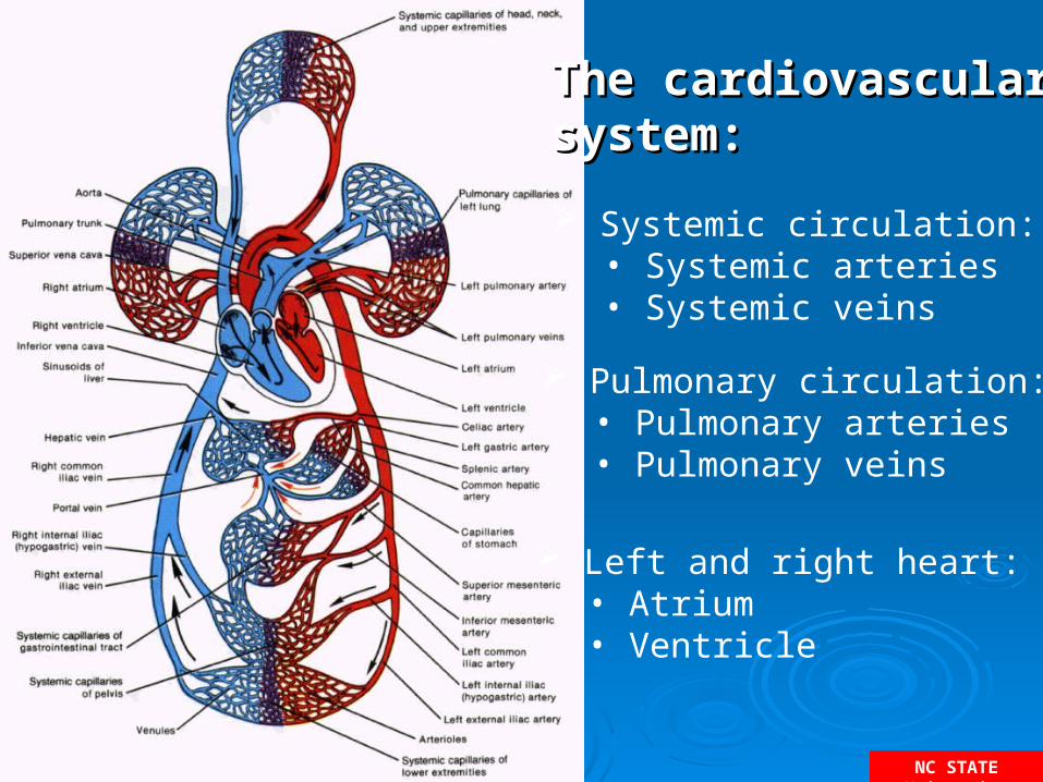
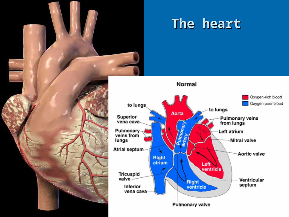
Pulmonary circulation:• Pulmonary arteries• Pulmonary veins

Left and right heart:• Atrium• Ventricle

The cardiovascular The cardiovascular system:system: Systemic circulation:

• Systemic arteries• Systemic veins

NC STATE University

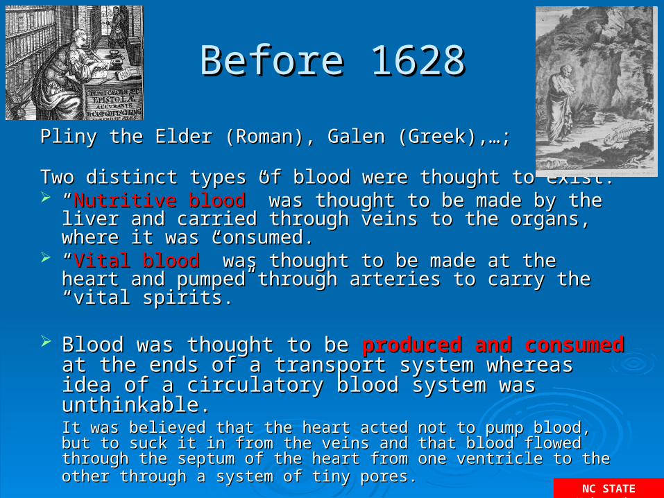
Before 1628Before 1628

Pliny the Elder (Roman), Galen (Greek),…;Pliny the Elder (Roman), Galen (Greek),…;

Two distinct types of blood were thought to exist:Two distinct types of blood were thought to exist: ““Nutritive bloodNutritive blood” was thought to be made by the liver and ” was thought to be made by the liver and

carried through veins to the organs, where it was carried through veins to the organs, where it was consumed. consumed.

““Vital bloodVital blood” was thought to be made at the heart and ” was thought to be made at the heart and pumped through arteries to carry the “vital spirits.” pumped through arteries to carry the “vital spirits.”

Blood was thought to be Blood was thought to be produced and consumedproduced and consumed at the ends of a transport system whereas idea of a at the ends of a transport system whereas idea of a circulatory blood system was unthinkable.circulatory blood system was unthinkable. It was believed that the heart acted not to pump blood, but to suck it It was believed that the heart acted not to pump blood, but to suck it in from the veins and that blood flowed through the septum of the in from the veins and that blood flowed through the septum of the heart from one ventricle to the other through a system of tiny pores.heart from one ventricle to the other through a system of tiny pores.

NC STATE University

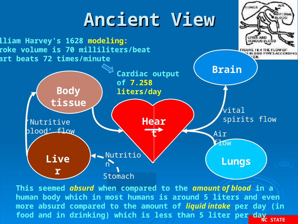
Ancient ViewAncient View

Liver

Body tissue

Heart

Lungs

Brain

Stomach

‘Nutritive blood‘ flow

vital spirits flow

Air flow

Nutrition

This seemed absurd when compared to the amount of blood in a human body which in most humans is around 5 liters and even more absurd compared to the amount of liquid intake per day (in food and in drinking) which is less than 5 liter per day

William Harvey’s 1628 modeling:Stroke volume is 70 milliliters/beatHeart beats 72 times/minute

Cardiac output of 7.258 liters/day

NC STATE University

• Modeling gave birth to the view that blood must Modeling gave birth to the view that blood must circulate. Harvey successfully announced the discovery circulate. Harvey successfully announced the discovery of the circulatory blood system.of the circulatory blood system.

• Harvey discovered the circulation of blood 46 year Harvey discovered the circulation of blood 46 year before the discovery of the light microscope.before the discovery of the light microscope.

• Consequently Harvey changed the view of the world Consequently Harvey changed the view of the world using a simple mathematical model making the using a simple mathematical model making the inaccessible accessible.inaccessible accessible.

1.1. In 1615 Harvey wrote (hand-written notes) that he was convinced that blood In 1615 Harvey wrote (hand-written notes) that he was convinced that blood circulated. circulated.

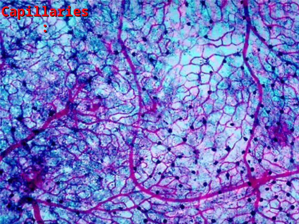
2.2. Anton Van Leeuwenhoek's microscope from 1674 (the first functioning light Anton Van Leeuwenhoek's microscope from 1674 (the first functioning light microscope) was sufficiently strong to make the capillaries visible.microscope) was sufficiently strong to make the capillaries visible.

3.3. Van Leeuwenhoek was the first to see and describe the capillaries of the Van Leeuwenhoek was the first to see and describe the capillaries of the circulatory system.circulatory system.

4.4. Marcello Malpighi, made the discovery simultaneously and independently, Marcello Malpighi, made the discovery simultaneously and independently, published his discovery of the capillaries in 1675. He is often credited the published his discovery of the capillaries in 1675. He is often credited the discovery of the capillaries by use of the microscope.discovery of the capillaries by use of the microscope.

NC STATE University

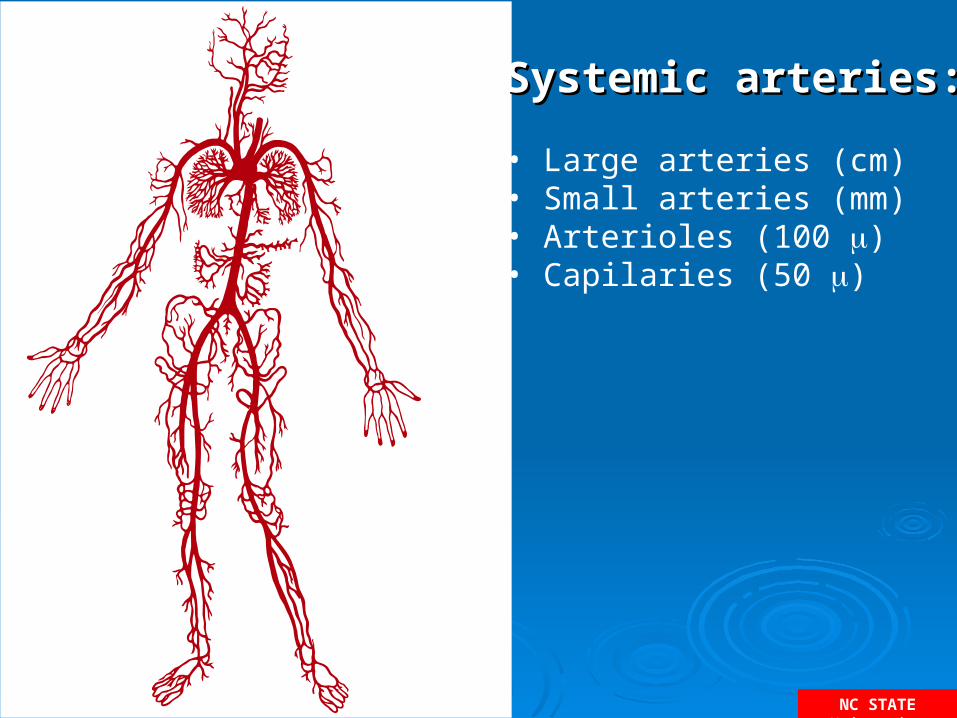
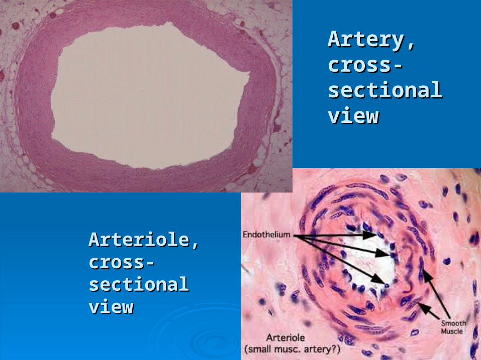
Systemic arteries:Systemic arteries:

• Large arteries (cm)• Small arteries (mm)• Arterioles (100 )• Capilaries (50 )

NC STATE University

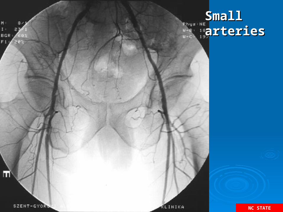
Small Small arteriesarteries

NC STATE University

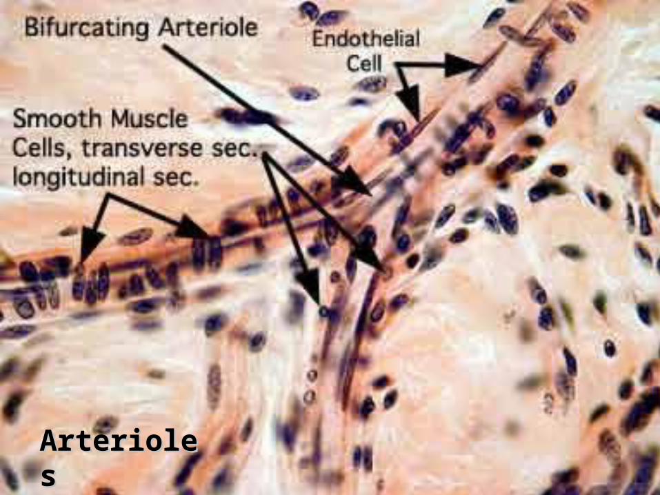
ArteriolesArterioles

NC STATE University

Capillaries:Capillaries:

NC STATE University

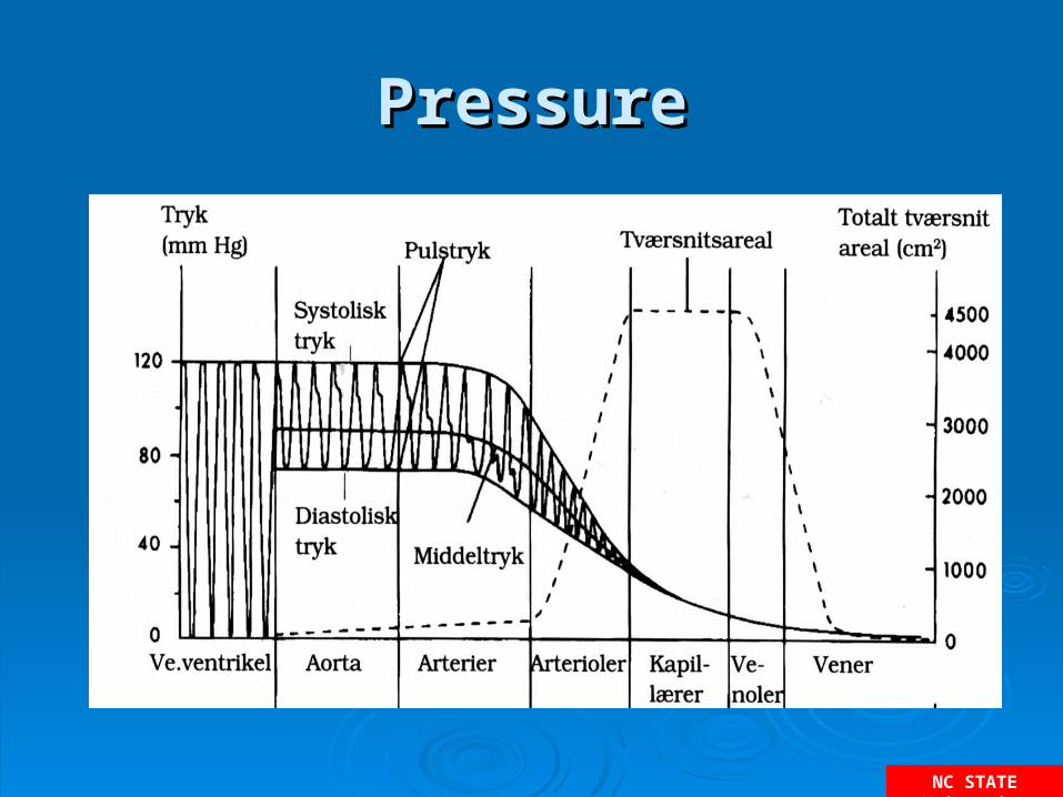
PressurePressure

NC STATE University

Artery, cross-Artery, cross-sectional viewsectional view

Arteriole, cross-Arteriole, cross-sectional viewsectional view

NC STATE University

The heartThe heart

NC STATE University

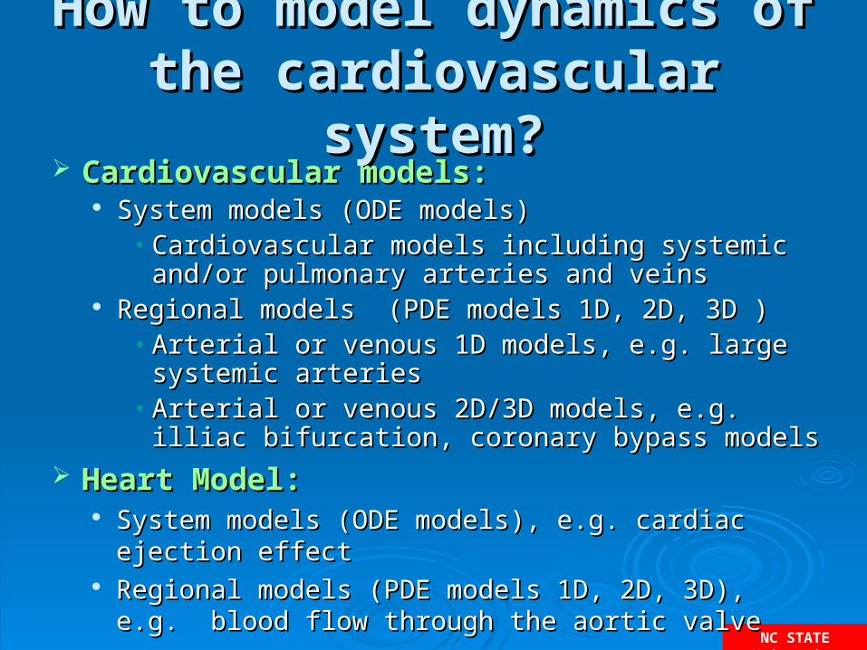
How to model dynamics of the How to model dynamics of the cardiovascular system?cardiovascular system?

Heart Model:Heart Model: System models (ODE models), e.g. cardiac ejection effect System models (ODE models), e.g. cardiac ejection effect Regional models (PDE models 1D, 2D, 3D), e.g. blood flow Regional models (PDE models 1D, 2D, 3D), e.g. blood flow

through the aortic valvethrough the aortic valve

Cardiovascular models:Cardiovascular models: System models (ODE models)System models (ODE models)

• Cardiovascular models including systemic and/or pulmonary Cardiovascular models including systemic and/or pulmonary arteries and veinsarteries and veins

Regional models (PDE models 1D, 2D, 3D )Regional models (PDE models 1D, 2D, 3D )• Arterial or venous 1D models, e.g. large systemic arteriesArterial or venous 1D models, e.g. large systemic arteries• Arterial or venous 2D/3D models, e.g. illiac bifurcation, Arterial or venous 2D/3D models, e.g. illiac bifurcation,

coronary bypass modelscoronary bypass models

NC STATE University

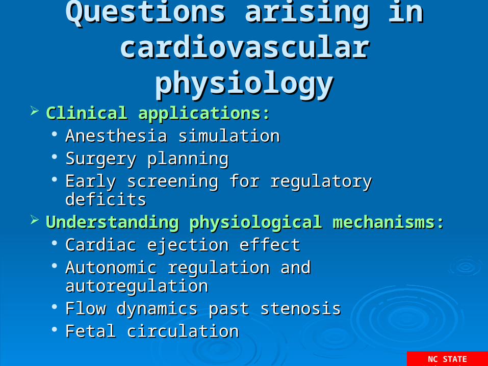
Questions arising in cardiovascular Questions arising in cardiovascular physiologyphysiology

Clinical applications:Clinical applications: Anesthesia simulation Anesthesia simulation Surgery planningSurgery planning Early screening for regulatory deficitsEarly screening for regulatory deficits

Understanding physiological mechanisms:Understanding physiological mechanisms: Cardiac ejection effectCardiac ejection effect Autonomic regulation and autoregulationAutonomic regulation and autoregulation Flow dynamics past stenosisFlow dynamics past stenosis Fetal circulationFetal circulation

NC STATE University

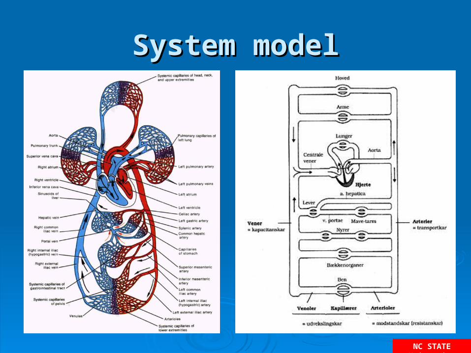
System modelSystem model

NC STATE University

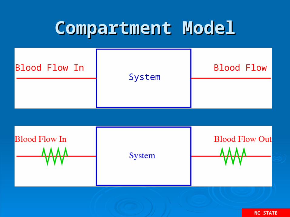
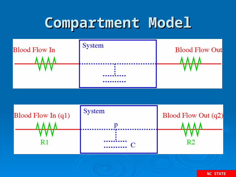
Compartment ModelCompartment Model

Blood Flow In Blood Flow OutSystem

Blood Flow Out

System

Blood Flow In

NC STATE University

Compartment ModelCompartment Model

Blood Flow In Blood Flow OutSystem

pBlood Flow Out (q2)

System

C R2R1

Blood Flow In (q1)

NC STATE University

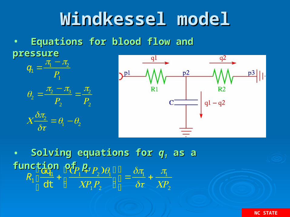
Windkessel modelWindkessel model

R1

dq1

dt+

(R1 + R2 )q1CR1R2

⎛

⎝⎜⎞

⎠⎟⎡

⎣⎢

⎤

⎦⎥=dp1dt

+p1CR2

• Solving equations for Solving equations for qq11 as a function of as a function of pp11

q1 =p1 −p2R1

q2 =p2 −p3R2

=p2R2

Cdp2dt

=q1 −q2

• Equations for blood flow and pressureEquations for blood flow and pressure

NC STATE University

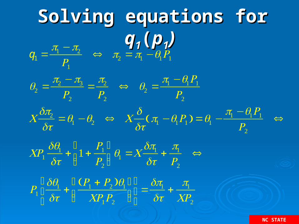
Solving equations for Solving equations for qq11((pp11))q1 =

p1 −p2R1

⇔ p2 =p1 −q1R1

q2 =p2 −p3R2

=p2R2

⇔ q2 =p1 −q1R1R2

Cdp2dt

=q1 −q2 ⇔ Cddtp1 −q1R1( ) =q1 −

p1 −q1R1R2

⇔

CR1dq1dt

+ 1+R1R2

⎛

⎝⎜⎞

⎠⎟q1 =C

dp1dt

+p1R2

⇔

R1dq1dt

+(R1 + R2 )q1CR1R2

⎛

⎝⎜⎞

⎠⎟⎡

⎣⎢

⎤

⎦⎥=dp1dt

+p1CR2

NC STATE University

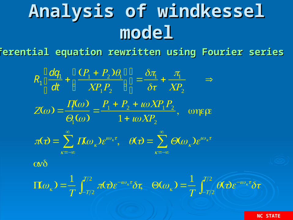
Analysis of windkessel modelAnalysis of windkessel model

R1

dq1

dt+

(R1 + R2 )q1CR1R2

⎛

⎝⎜⎞

⎠⎟⎡

⎣⎢

⎤

⎦⎥=dp1dt

+p1CR2

⇒

Z(ω) =P1(ω)Q1(ω)

=R1 + R2 + iωCR1R2

1+ iωCR2, where

p(t) = P(ωk)eiωkt,

k=−∞

∞

∑ q(t) = Q(ωk)eiωkt

k=−∞

∞

∑and

P(ωk) =1T

p(t)e−iωkt−T 2

T 2

∫ dt, Q(ωk) =1T

q(t)e−iωkt−T 2

T 2

∫ dt

• Differential equation rewritten using Fourier seriesDifferential equation rewritten using Fourier series

NC STATE University

Analysis of windkessel modelAnalysis of windkessel model

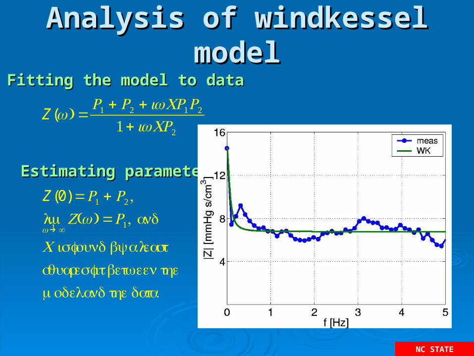
Z(ω) =R1 + R2 + iωCR1R2

1+ iωCR2

• Fitting the model to dataFitting the model to data

• Estimating parametersEstimating parameters

Z(0) =R1 + R2 , limω→ ∞Z(ω) =R1, and

C is found by a least squares fit between the model and the data

NC STATE University

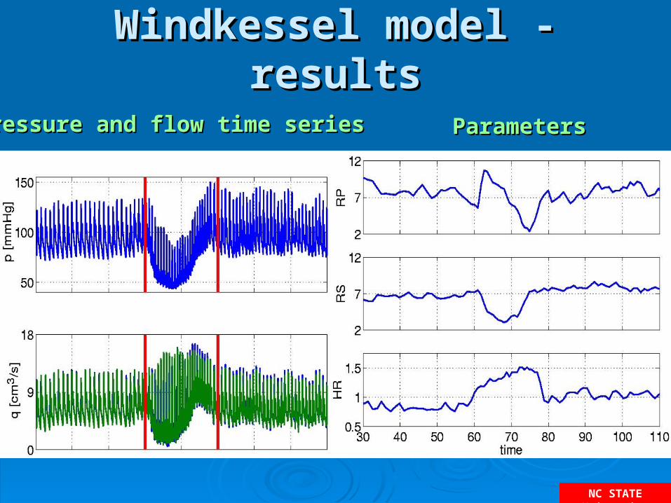
Windkessel model - resultsWindkessel model - results

Pressure and flow time seriesPressure and flow time series ParametersParameters

NC STATE University

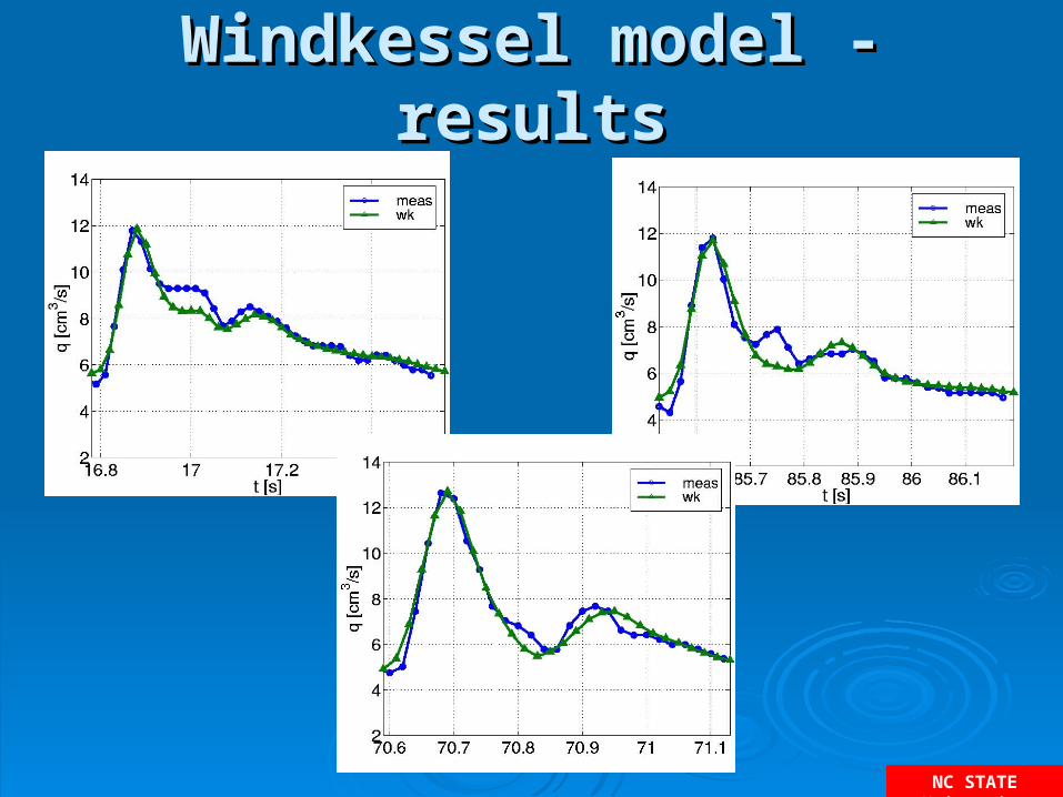
Windkessel model - resultsWindkessel model - results

NC STATE University

NC STATE University

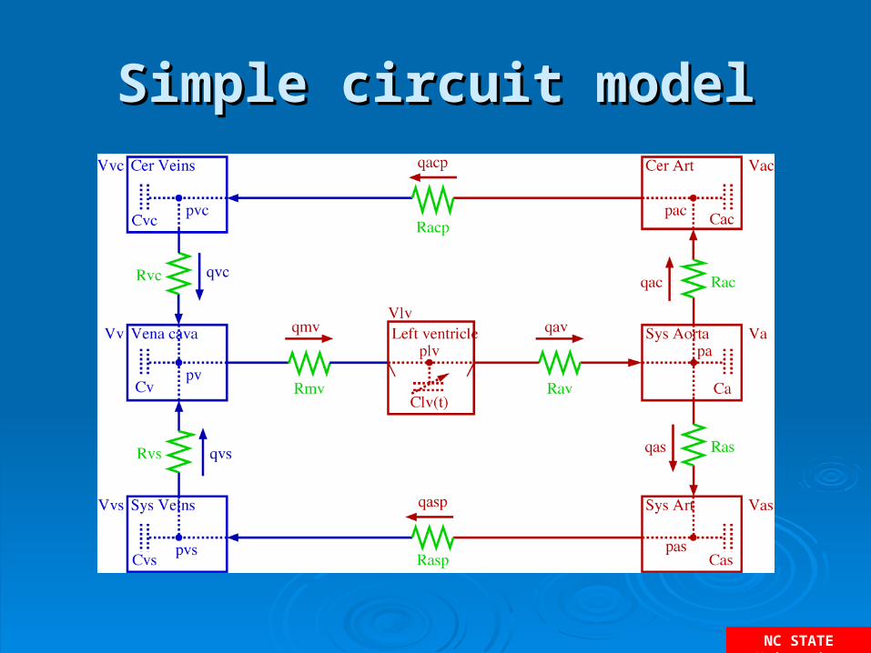
Simple circuit modelSimple circuit model

NC STATE University

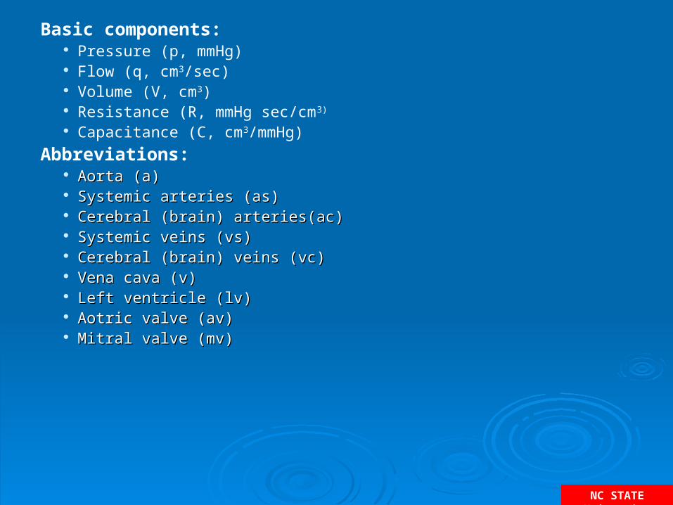
Basic components: Pressure (p, mmHg) Flow (q, cm3/sec) Volume (V, cm3) Resistance (R, mmHg sec/cm3)

Capacitance (C, cm3/mmHg)

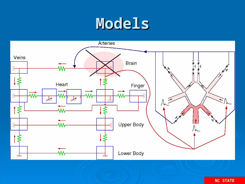
Abbreviations: Aorta (a)Aorta (a) Systemic arteries (as)Systemic arteries (as) Cerebral (brain) arteries(ac)Cerebral (brain) arteries(ac) Systemic veins (vs)Systemic veins (vs) Cerebral (brain) veins (vc)Cerebral (brain) veins (vc) Vena cava (v)Vena cava (v) Left ventricle (lv)Left ventricle (lv) Aotric valve (av)Aotric valve (av) Mitral valve (mv)Mitral valve (mv)

NC STATE University

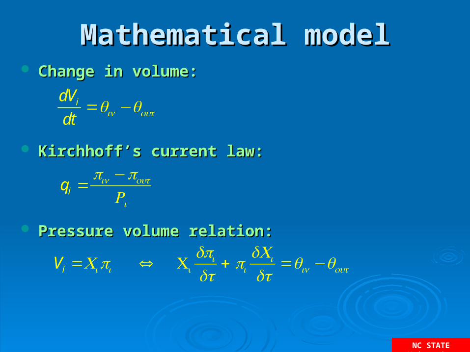
Mathematical modelMathematical model Change in volume:Change in volume:

Kirchhoff’s current law: Kirchhoff’s current law:

Pressure volume relation:Pressure volume relation:

dVi

dt=qin−qout

qi =pin−poutRi

Vi =Cipi ⇔ Cidpidt

+ pidCidt

=qin−qout

NC STATE University

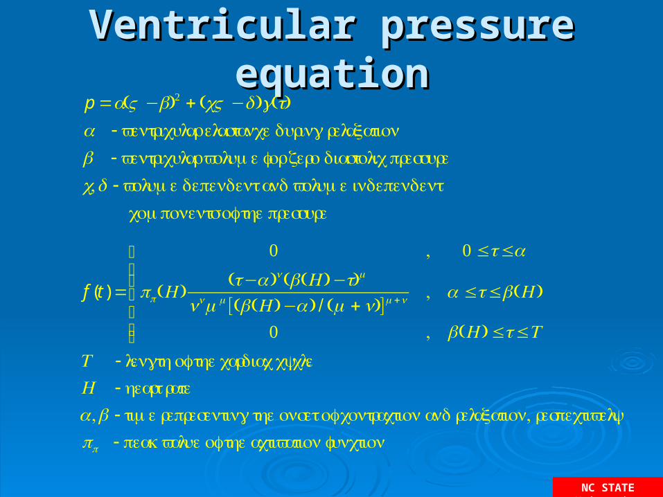
Ventricular pressure equationVentricular pressure equationp =a(V−b)2 + (cV−d)g(t)a - ventricular elastance during relaxationb - ventricular volume for zero diastolic pressurec,d - volume dependent and volume independent components of the pressure

f (t) =

0 , 0 ≤t≤α

pp(H )(t−α)n(β(H )−t)m

nnmm[(β(H )−α) / (m+n)]m+n, α ≤t≤β(H )

0 , β(H ) ≤t≤T

⎧

⎨⎪⎪

⎩⎪⎪

T - length of the cardiac cycleH - heart rateα,β - time representing the onset of contraction and relaxation, respectivelypp - peak value of the activation function

NC STATE University

Ca

dpa

dt=qav−qas−qac−pa

dCadt

Casdpasdt

=qas−qasp−pasdCasdt

Cacdpacdt

=qac−qacp−pacdCacdt

Cvsdpvsdt

=qasp−qvs−pvsdCvsdt

Cvcdpvcdt

=qacp−qvc−pvcdCvcdt

Cvdpvdt

=qvs +qvc−qmv−pvdCvdt

dVlvdt

=qmv−qau

NC STATE University

Model parametersModel parameters

R: R: Rmv, Rav, Ras, Rac, Rasp, Racp, Rvs, RvcRmv, Rav, Ras, Rac, Rasp, Racp, Rvs, Rvc

C:C: Ca, Cas, Cac, Cv, Cvs, CvcCa, Cas, Cac, Cv, Cvs, Cvc

Heart parameters:Heart parameters: a, b, c, d, n, m, tmax, tmin, pmax, pmin, nu, a, b, c, d, n, m, tmax, tmin, pmax, pmin, nu,

mu, theta, phimu, theta, phi

NC STATE University

Model parameters - Initial Model parameters - Initial valuesvalues

NC STATE University

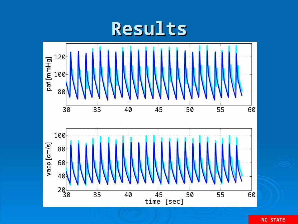
Model parametersModel parameters Initial parameters obtained from literature dataInitial parameters obtained from literature data Optimal parameters obtained using non-linear optimization Optimal parameters obtained using non-linear optimization

minimizing the error between computed and measured minimizing the error between computed and measured valuesvalues

J =α1

pa−pad2∑

Npa+α2

vacp−vacpd2

∑Nvacp

+α 3

pa,sys−pad,sys2

∑Npa,sys

+α 4

pa,dia−pad,dia2∑

Npad,dia

+α5

vacp,sys−vacpd,sys2

∑Nvacp,sys

+α6

vacp,dia−vacpd,dia2

∑Nvacp,dia

NC STATE University

ResultsResults

30 35 40 45 50 55 60

80

100

120

30 35 40 45 50 55 6020

40

60

80

100

time [sec]

NC STATE University

Inductors - Laplace analogyInductors - Laplace analogy

NC STATE University

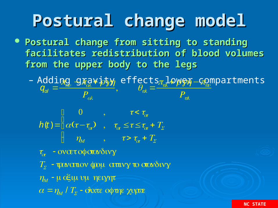
Postural change modelPostural change model Postural change from sitting to standing facilitates redistribution of Postural change from sitting to standing facilitates redistribution of

blood volumes from the upper body to the legsblood volumes from the upper body to the legs

– Adding gravity effects lower compartments

h(t) =0 , t < tst

α(t−tst) , tst ≤t≤tst +TShM , t > tst +TS

⎧

⎨⎪

⎩⎪

tst - onset of standingTS - transition from sitting to standinghM - maximum height α =hM /TS - slope of the curve

qal =pau−pal + ρgh

Ral, qvl =

pvl + ρgh−pvuRvl

NC STATE University

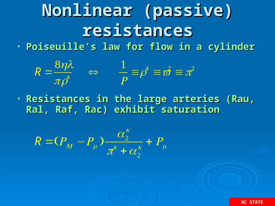
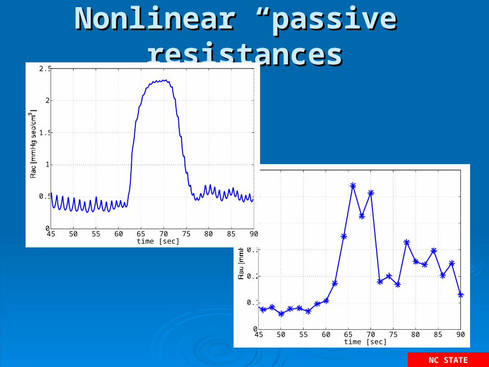
Nonlinear (passive) resistancesNonlinear (passive) resistances• Poiseuille’s law for flow in a cylinderPoiseuille’s law for flow in a cylinder

• Resistances in the large arteries (Rau, Ral, Raf, Rac) Resistances in the large arteries (Rau, Ral, Raf, Rac) exhibit saturationexhibit saturation

R =8ηlπr4

⇔ 1R≡r4 ≡v2 ≡p2

R =(RM −Rm)α2k

pk +α2k + Rm

NC STATE University

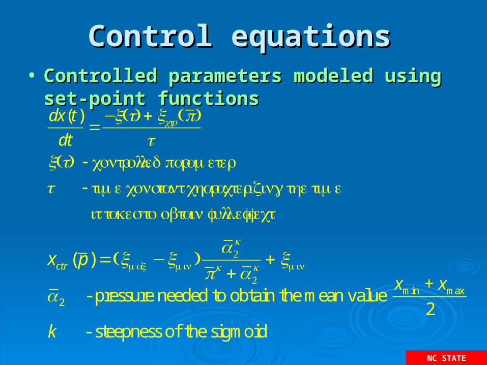
Control equationsControl equations• Controlled parameters modeled using set-point functionsControlled parameters modeled using set-point functions

dx(t)

dt=−x(t) + xctr (p)

τx(t) - controlled parameterτ - time constant characterizing the time it takes to obtain full effect

xctr (p) =(xmax −xmin)α2k

pk +α2k + xmin

α2 - pressure needed to obtain the mean value xmin + xmax

2k - steepness of the sigmoid

NC STATE University

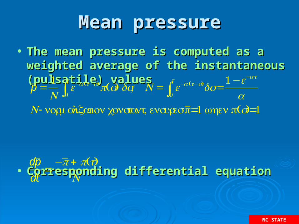
Mean pressureMean pressure

• The mean pressure is computed as a weighted average of The mean pressure is computed as a weighted average of the instantaneous (pulsatile) valuesthe instantaneous (pulsatile) values

• Corresponding differential equationCorresponding differential equation

p =1Ne−α(t−s)

0

t

∫ p(s) ds, N = e−α(t−s)

0

t

∫ ds=1−e−αt

αN- normalization constant, ensures p=1 when p(s)=1

dp

dt=−p+ p(t)N

NC STATE University

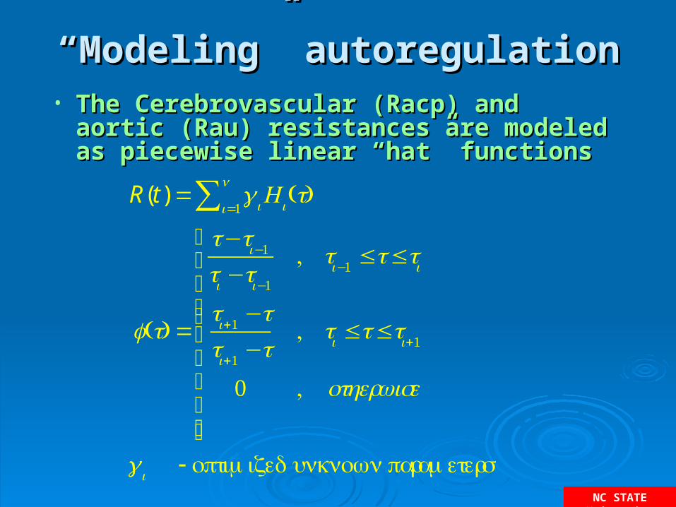
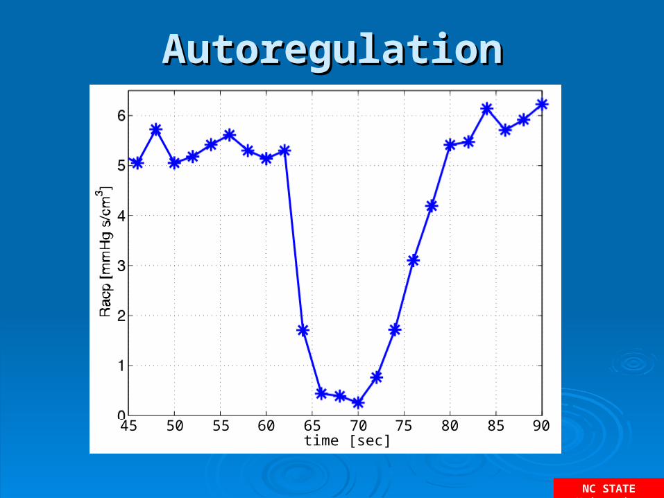
““Modeling” autoregulationModeling” autoregulation

R(t) = γiHi (t)i=1

n∑

f (t) =

t−ti−1ti −ti−1

, ti−1 ≤t≤ti

ti+1 −tti+1 −t

, ti ≤t≤ti+1

0 , otherwise

⎧

⎨

⎪⎪⎪⎪

⎩

⎪⎪⎪⎪

γi - optimized unknown parameters

• The Cerebrovascular (Racp) and aortic (Rau) The Cerebrovascular (Racp) and aortic (Rau) resistances are modeled as piecewise linear “hat” resistances are modeled as piecewise linear “hat” functionsfunctions

NC STATE University

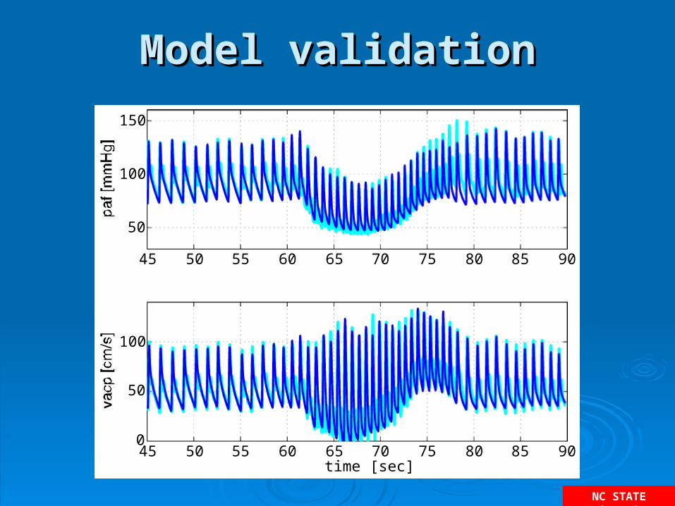
Model validationModel validation

45 50 55 60 65 70 75 80 85 90

50

100

150

45 50 55 60 65 70 75 80 85 900

50

100

time [sec]

NC STATE University

Model parametersModel parameters

Uncontrolled parametersUncontrolled parameters, , resistances and capacitors used from resistances and capacitors used from steady state simulation.steady state simulation.

Controlled parametersControlled parameters, , gravity and non-linear resistances, gravity and non-linear resistances, regulated resistances and capacitors, and autoregulation regulated resistances and capacitors, and autoregulation equation give rise to 110 parameters.equation give rise to 110 parameters.

Parameters identifiedParameters identified using Nelder-Mead non-linear using Nelder-Mead non-linear optimization to identify parameters that minimize the error optimization to identify parameters that minimize the error between data and model.between data and model.

Uncontrolled parametersUncontrolled parameters, , resistances and capacitors used from resistances and capacitors used from steady state simulation.steady state simulation.

Controlled parametersControlled parameters, , gravity and non-linear resistances, gravity and non-linear resistances, regulated resistances and capacitors, and autoregulation regulated resistances and capacitors, and autoregulation equation give rise to 110 parameters.equation give rise to 110 parameters.

Parameters identifiedParameters identified using Nelder-Mead non-linear using Nelder-Mead non-linear optimization to identify parameters that minimize the error optimization to identify parameters that minimize the error between data and model.between data and model.

NC STATE University

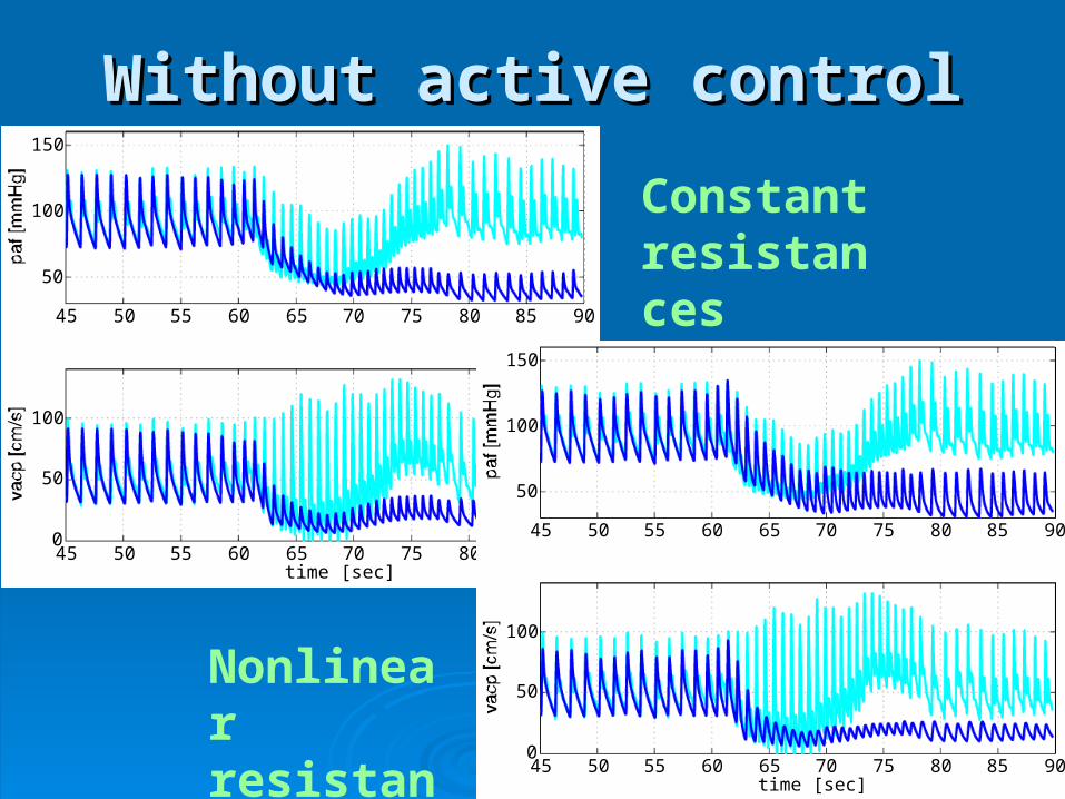
Without active controlWithout active control

45 50 55 60 65 70 75 80 85 90

50

100

150

45 50 55 60 65 70 75 80 85 900

50

100

time [sec]

Constant resistances

45 50 55 60 65 70 75 80 85 90

50

100

150

45 50 55 60 65 70 75 80 85 900

50

100

time [sec]

Nonlinear resistances

NC STATE University

Nonlinear “passive” resistancesNonlinear “passive” resistances

45 50 55 60 65 70 75 80 85 900

0.1

0.2

0.3

0.4

0.5

time [sec]

45 50 55 60 65 70 75 80 85 900

0.5

1

1.5

2

2.5

time [sec]

NC STATE University

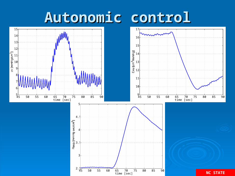
Autonomic controlAutonomic control

45 50 55 60 65 70 75 80 85 905

6

7

8

9

10

11

12

13

14

15

time [sec]45 50 55 60 65 70 75 80 85 909

10

11

12

13

14

15

16

17

time [sec]

45 50 55 60 65 70 75 80 85 902.5

3

3.5

4

4.5

5

time [sec]

NC STATE University

AutoregulationAutoregulation

45 50 55 60 65 70 75 80 85 900

1

2

3

4

5

6

time [sec]

NC STATE University

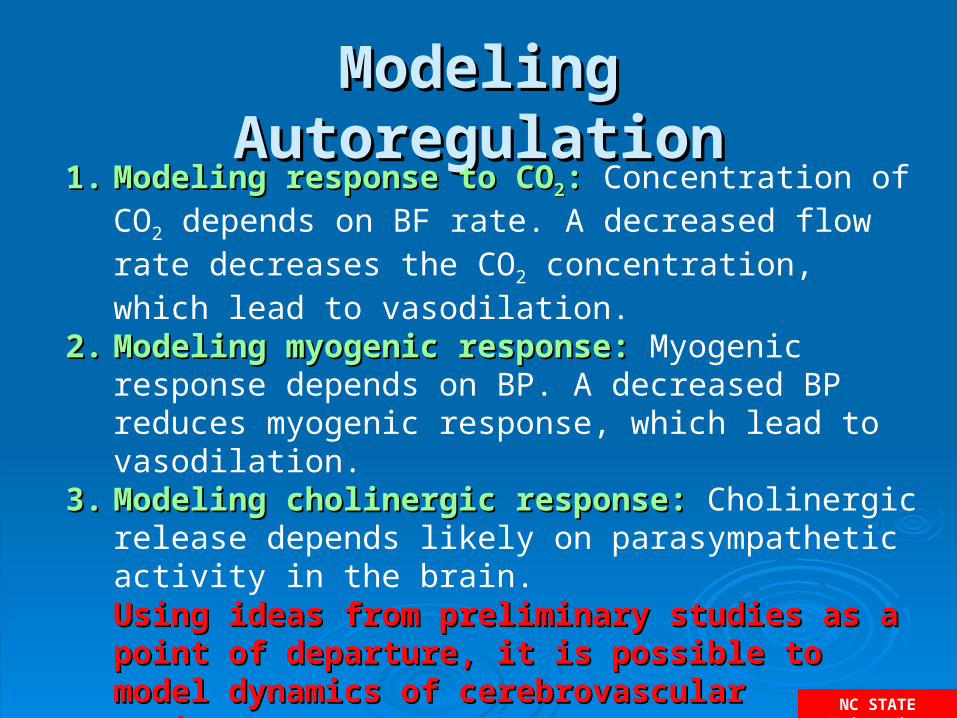
Modeling AutoregulationModeling Autoregulation1.1. Modeling response to COModeling response to CO22: : Concentration of

CO2 depends on BF rate. A decreased flow rate decreases the CO2 concentration, which lead to vasodilation.

2.2. Modeling myogenic response:Modeling myogenic response: Myogenic response depends on BP. A decreased BP reduces myogenic response, which lead to vasodilation.

3.3. Modeling cholinergic response: Modeling cholinergic response: Cholinergic release depends likely on parasympathetic activity in the brain.Using ideas from preliminary studies as a Using ideas from preliminary studies as a point of departure, it is possible to point of departure, it is possible to model dynamics of cerebrovascular model dynamics of cerebrovascular resistance.resistance.

NC STATE University

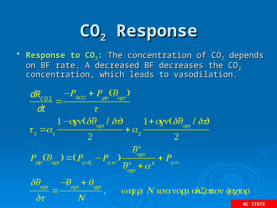
COCO22 Response Response Response to COResponse to CO22: : The concentration of COThe concentration of CO22 depends on BF depends on BF

rate. A decreased BF decreases the COrate. A decreased BF decreases the CO22 concentration, which concentration, which leads to vasodilation.leads to vasodilation.

dRCO2

dt=−RCO2 + Rctr (qacp)

τ

τ 3 =α1

1−sgn(dqacp / dt)

2+α2

1+sgn(dqacp / dt)

2

Rctr (qacp) =(Rmax −Rmin)qacpk

qacpk +α k

+ Rmin

dqacpdt

=−qacp +qacpN

, where N is a normalization factor

NC STATE University

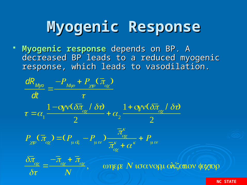
Myogenic ResponseMyogenic Response Myogenic responseMyogenic response depends on BP. A decreased BP depends on BP. A decreased BP

leads to a reduced myogenic response, which leads to leads to a reduced myogenic response, which leads to vasodilation.vasodilation.

dRMyo

dt=−RMyo + Rctr (pac)

τ

τ =α1

1−sgn(dpac / dt)2

+α2

1+sgn(dpac / dt)2

Rctr (pac) =(Rmax −Rmin)pack

pack +α k

+ Rmin

dpacdt

=−pac + pacN

, where N is a normalization factor

NC STATE University

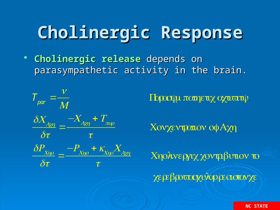
Cholinergic ResponseCholinergic Response

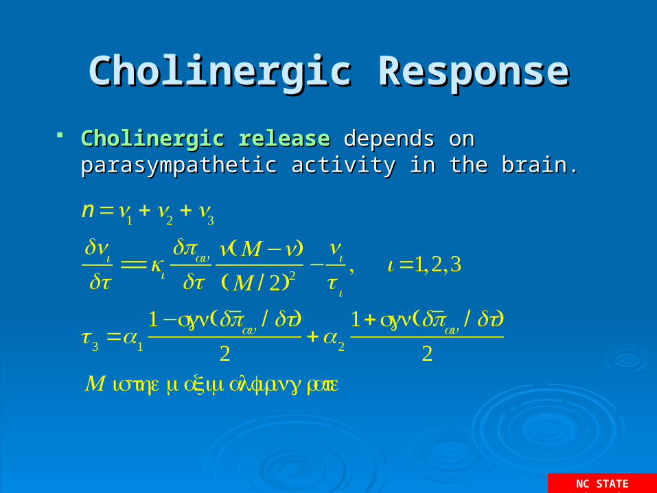
Cholinergic releaseCholinergic release depends on parasympathetic depends on parasympathetic activity in the brain.activity in the brain.

n =n1 +n2 +n3dnidt

==kidpaudtn(M −n)(M / 2)2

−niτ i

, i=1,2,3

τ 3 =α1

1−sgn(dpau / dt)2

+α2

1+sgn(dpau / dt)2

M is the maximal firing rate

NC STATE University

Cholinergic ResponseCholinergic Response

Tpar

=nM

Parasympathetic activity

dCAchdt

=−CAch +Tpar

τ Concentration of Ach

dRChodt

=−RCho + kChoCAch

τ Cholinergic contribution to

cerebrovascular resistance

Cholinergic releaseCholinergic release depends on parasympathetic depends on parasympathetic activity in the brain.activity in the brain.

NC STATE University

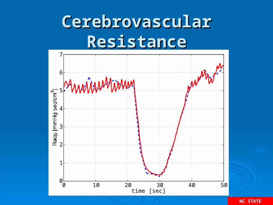
Cerebrovascular ResistanceCerebrovascular Resistance

0 10 20 30 40 500

1

2

3

4

5

6

7

time [sec]

NC STATE University

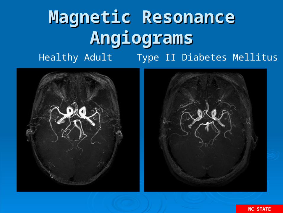
Magnetic Resonance Magnetic Resonance AngiogramsAngiograms

Healthy Adult Type II Diabetes Mellitus

NC STATE University

ModelsModels

NC STATE University

ReferencesReferences Olufsen, Nadim & Lipsitz L. Dynamics of cerebral blood flow

regulation explained using a lumped parameter model. Am J Physiol 282: R611-R622, 2002.

Olufsen, Ottesen, Tran, Ellwein, Lipsitz & Novak. Blood pressure and blood flow variation during postural change from sitting to standing: model development and validation. J Appl Physiol 99: 1523-1537, 2005.

Olufsen, Tran, Ottesen, REU program, Lipsitz & Nova. Modeling baroreflex regulation of heart rate during orthostatic stress. Am J Physiol in press, 2006.

Ottesen, Olufsen & Larsen. Applied Mathematical Models in Human Physiology: SIAM, 2004.

Guyton &Hall. Textbook of medical physiology. Philadelphia: WB Saunders, 1996.

Edvinsson & Krause. Cerebral Blood Flow and Metabolism. Philadelphia: Lippincott Williams and Wilkins, 2002.

NC STATE University

AcknowledgementsAcknowledgements• CollaboratorsCollaborators

– Hien Tran, Deptartment of Math, NCSUHien Tran, Deptartment of Math, NCSU– Joel Trussell, Dept of Electrical Engineering, NCSUJoel Trussell, Dept of Electrical Engineering, NCSU– Lewis Lipsitz, HRCA & Harvard Medical School, BostonLewis Lipsitz, HRCA & Harvard Medical School, Boston– Vera Novak, BIDMC & Harvard Medical School, BostonVera Novak, BIDMC & Harvard Medical School, Boston– Johnny Ottesen, Dept of Math, Roskilde University, DenmarkJohnny Ottesen, Dept of Math, Roskilde University, Denmark– Ali Nadim, The Keck Institute and Claremont Graduate UniversityAli Nadim, The Keck Institute and Claremont Graduate University– Charles Peskin, Courant Institute of Mathematical SciencesCharles Peskin, Courant Institute of Mathematical Sciences– Jesper Larsen, Dept of Math, Roskilde University, DenmarkJesper Larsen, Dept of Math, Roskilde University, Denmark– Stig Andur Pedersen, Dept of Phil, Roskilde University, DenmarkStig Andur Pedersen, Dept of Phil, Roskilde University, Denmark

• StudentsStudents– Cynthia Chmielewski, Laura Ellwein, Anna HartCynthia Chmielewski, Laura Ellwein, Anna Hart– Daniela (M), Dave (M/Stat), Mark (M/P), Dave H (M), Derek (EE)Daniela (M), Dave (M/Stat), Mark (M/P), Dave H (M), Derek (EE)

• Funding agenciesFunding agencies– NSF, NIH/NIA, and FRPD North Carolina State UniversityNSF, NIH/NIA, and FRPD North Carolina State University

NC STATE University

1.1. Using a mathematical model to Using a mathematical model to predict blood flow after bypass predict blood flow after bypass surgerysurgery

2.2. Understanding mechanisms Understanding mechanisms behind cerebral blood flow behind cerebral blood flow regulationregulation

NC STATE University

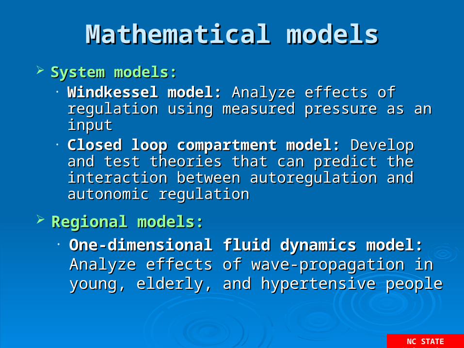
Mathematical modelsMathematical models

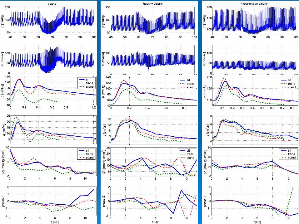
Regional models:Regional models:• One-dimensional fluid dynamics model:One-dimensional fluid dynamics model: Analyze Analyze

effects of wave-propagation in young, elderly, and effects of wave-propagation in young, elderly, and hypertensive peoplehypertensive people

System models:System models:• Windkessel model:Windkessel model: Analyze effects of regulation using Analyze effects of regulation using

measured pressure as an input measured pressure as an input • Closed loop compartment model:Closed loop compartment model: Develop and test Develop and test

theories that can predict the interaction between theories that can predict the interaction between autoregulation and autonomic regulationautoregulation and autonomic regulation

NC STATE University

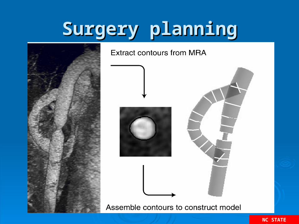
Surgery planningSurgery planning

NC STATE University

Surgery planningSurgery planning

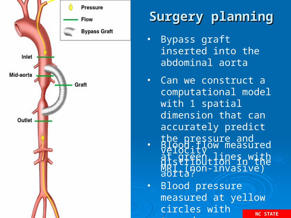
• Blood flow measured at green lines with MRI (non-invasive)

• Blood pressure measured at yellow circles with transducer (invasive)

• Bypass graft inserted into the abdominal aorta

• Can we construct a computational model with 1 spatial dimension that can accurately predict the pressure and velocity distribution in the aorta?

NC STATE University

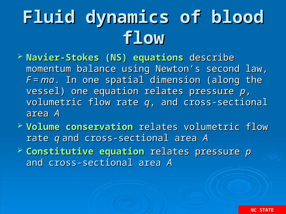
Fluid dynamics of blood flowFluid dynamics of blood flow

Navier-Stokes (NS) equationsNavier-Stokes (NS) equations describe momentum describe momentum balance using Newton’s second law, balance using Newton’s second law, F = maF = ma. In one spatial . In one spatial dimension (along the vessel) one equation relates pressure dimension (along the vessel) one equation relates pressure pp, volumetric flow rate , volumetric flow rate qq, and cross-sectional area , and cross-sectional area AA

Volume conservationVolume conservation relates volumetric flow rate relates volumetric flow rate q q and and cross-sectional area cross-sectional area AA

Constitutive equationConstitutive equation relates pressure relates pressure p p and cross-and cross-sectional area sectional area AA

NC STATE University

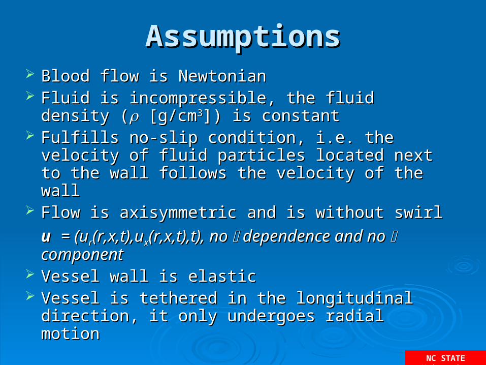
AssumptionsAssumptions Blood flow is NewtonianBlood flow is Newtonian Fluid is incompressible, the fluid density (Fluid is incompressible, the fluid density (ρρ

[g/cm[g/cm33]) is constant]) is constant Fulfills no-slip condition, i.e. the velocity of fluid Fulfills no-slip condition, i.e. the velocity of fluid

particles located next to the wall follows the particles located next to the wall follows the velocity of the wall velocity of the wall

Flow is axisymmetric and is without swirl Flow is axisymmetric and is without swirl

uu = (u= (urr(r,x,t),u(r,x,t),uxx(r,x,t),t), no (r,x,t),t), no dependence and no dependence and no component component

Vessel wall is elasticVessel wall is elastic Vessel is tethered in the longitudinal direction, it Vessel is tethered in the longitudinal direction, it

only undergoes radial motiononly undergoes radial motion

NC STATE University

AssumptionsAssumptions

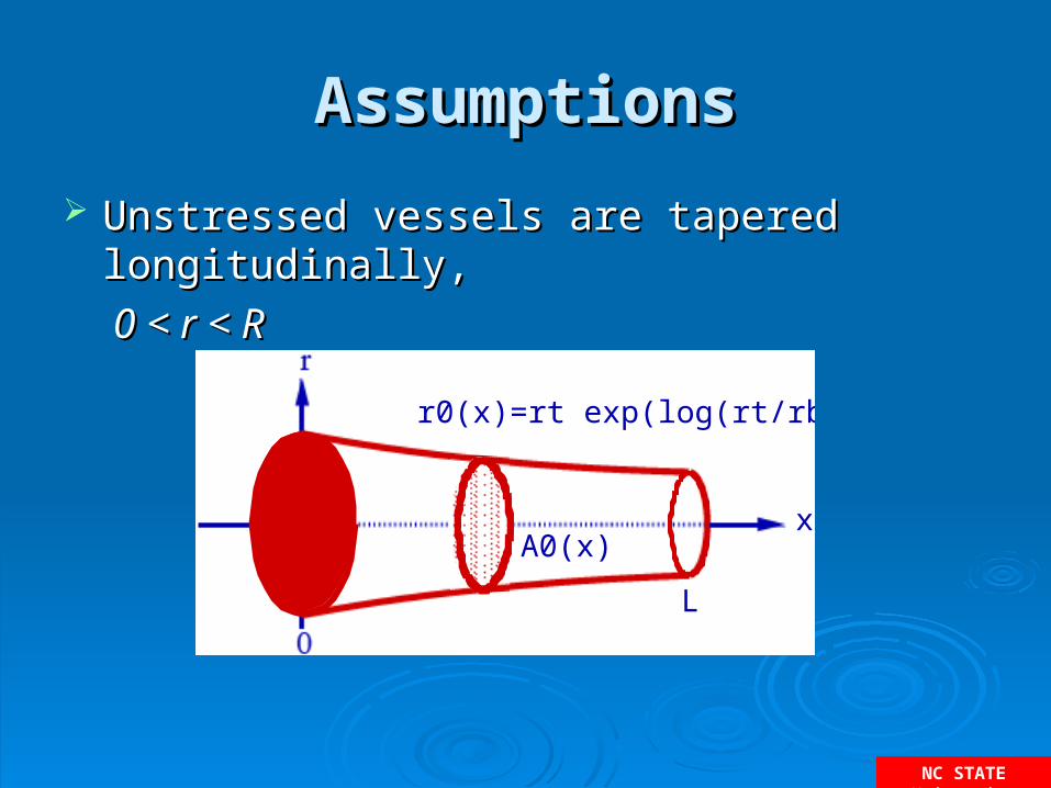
Unstressed vessels are tapered longitudinally,Unstressed vessels are tapered longitudinally,

0 < r < R0 < r < R

r

L

x

r0(x)=rt exp(log(rt/rb)x/L)

A0(x)

NC STATE University

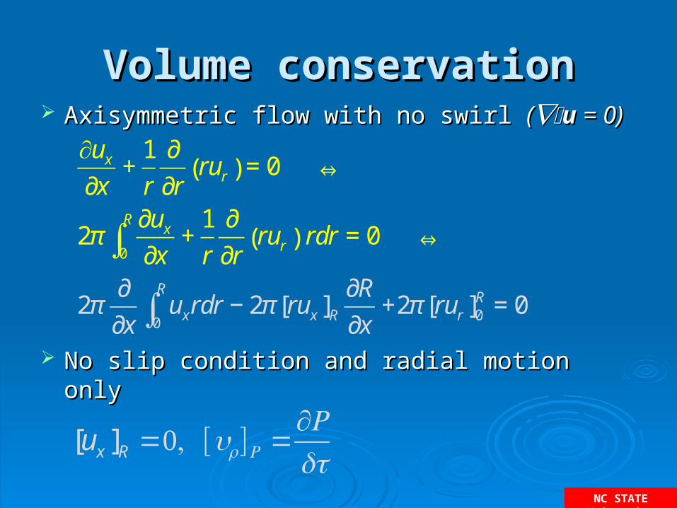
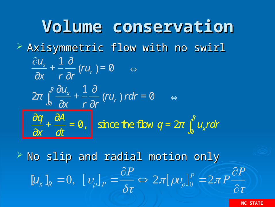
Volume conservationVolume conservation Axisymmetric flow with no swirl Axisymmetric flow with no swirl ((u u = 0)= 0)

No slip condition and radial motion onlyNo slip condition and radial motion only

∂ux

∂x+

1

r

∂

∂rrur( ) = 0 ⇔

2π∂ux

∂x+

1

r

∂

∂rrur( )

0

R

∫ rdr = 0 ⇔

2π∂

∂xuxrdr − 2π [rux ]R

∂R

∂x+

0

R

∫ 2π [rur ]0R = 0

[ux ]R =0, [ur ]R =∂Rdt

NC STATE University

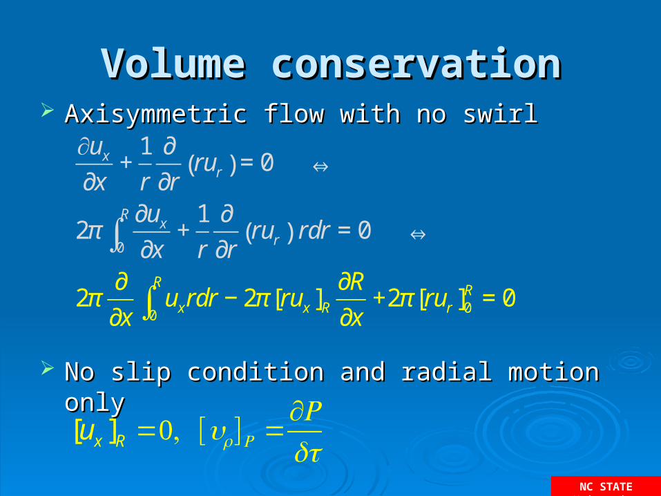
Volume conservationVolume conservation Axisymmetric flow with no swirlAxisymmetric flow with no swirl

No slip condition and radial motion onlyNo slip condition and radial motion only

∂ux

∂x+

1

r

∂

∂rrur( ) = 0 ⇔

2π∂ux

∂x+

1

r

∂

∂rrur( )

0

R

∫ rdr = 0 ⇔

2π∂

∂xuxrdr − 2π [rux ]R

∂R

∂x+

0

R

∫ 2π [rur ]0R = 0

[ux ]R =0, [ur ]R =∂Rdt

NC STATE University

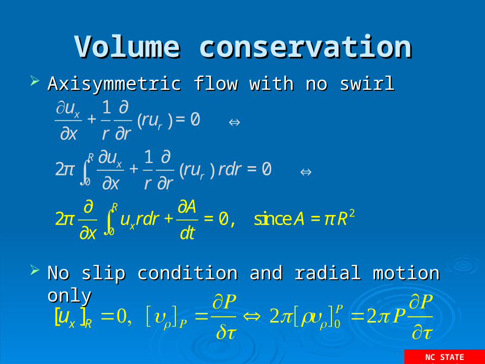
Volume conservationVolume conservation Axisymmetric flow with no swirlAxisymmetric flow with no swirl

No slip condition and radial motion onlyNo slip condition and radial motion only

∂ux

∂x+

1

r

∂

∂rrur( ) = 0 ⇔

2π∂ux

∂x+

1

r

∂

∂rrur( )

0

R

∫ rdr = 0 ⇔

2π∂

∂xuxrdr +

0

R

∫∂A

dt= 0, since A = π R2

[ux ]R =0, [ur ]R =∂Rdt

⇔ 2π[rur ]0R =2πR

∂R∂t

NC STATE University

Volume conservationVolume conservation Axisymmetric flow with no swirlAxisymmetric flow with no swirl

No slip and radial motion onlyNo slip and radial motion only

∂ux

∂x+

1

r

∂

∂rrur( ) = 0 ⇔

2π∂ux

∂x+

1

r

∂

∂rrur( )

0

R

∫ rdr = 0 ⇔

∂q

∂x+

∂A

dt= 0, since the flow q = 2π uxr0

R

∫ dr

[ux ]R =0, [ur ]R =∂Rdt

⇔ 2π[rur ]0R =2πR

∂R∂t

NC STATE University

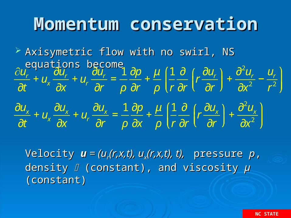
Momentum conservationMomentum conservation Axisymetric flow with no swirl, NS equations becomeAxisymetric flow with no swirl, NS equations become

Velocity Velocity u u = (u= (urr(r,x,t), u(r,x,t), uxx(r,x,t), t), (r,x,t), t), pressure pressure pp, density , density (constant), and viscosity (constant), and viscosity µµ (constant) (constant)

∂ur

∂t+ ux

∂ur

∂x+ ur

∂ur

∂r=

1

ρ

∂p

∂r+

μ

ρ

1

r

∂

∂rr

∂ur

∂r⎛⎝⎜

⎞⎠⎟

+∂2ur

∂x2−

ur

r2

⎛

⎝⎜⎞

⎠⎟

∂ux

∂t+ ux

∂ux

∂x+ ur

∂ux

∂r=

1

ρ

∂p

∂x+

μ

ρ

1

r

∂

∂rr

∂ux

∂r⎛⎝⎜

⎞⎠⎟

+∂2ux

∂x2

⎛

⎝⎜⎞

⎠⎟

NC STATE University

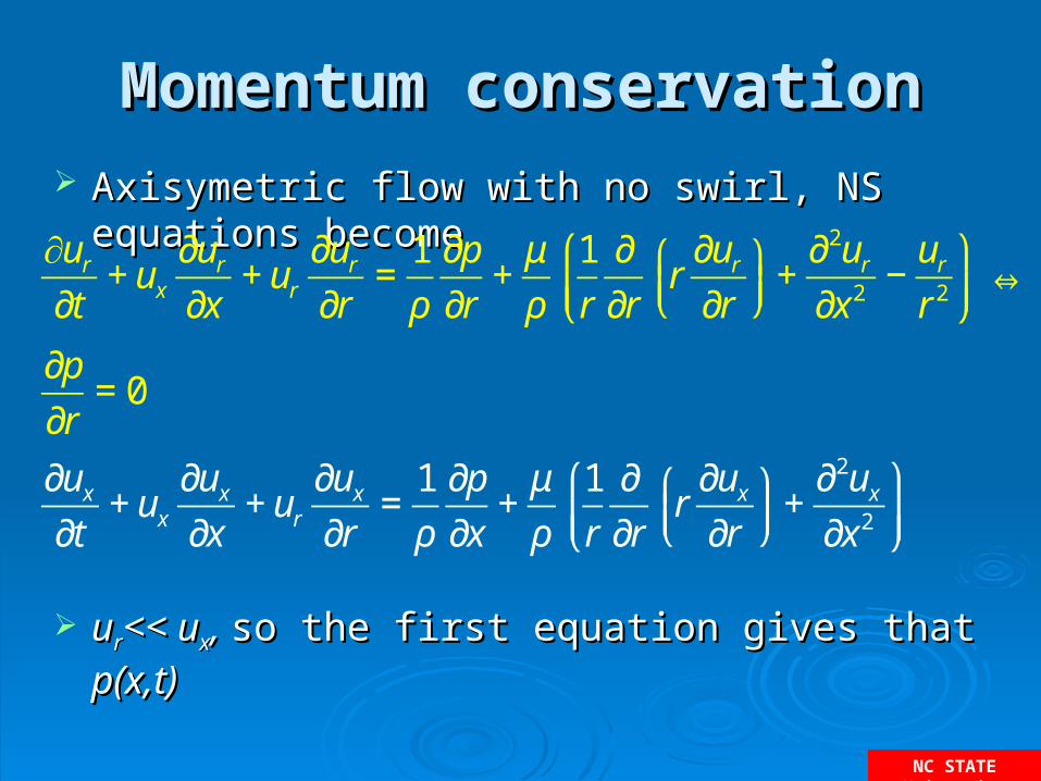
Momentum conservationMomentum conservation Axisymetric flow with no swirl, NS equations becomeAxisymetric flow with no swirl, NS equations become

uurr<< u<< uxx, , so the first equation gives that so the first equation gives that p(x,t)p(x,t)

∂ur

∂t+ ux

∂ur

∂x+ ur

∂ur

∂r=

1

ρ

∂p

∂r+

μ

ρ

1

r

∂

∂rr

∂ur

∂r⎛⎝⎜

⎞⎠⎟

+∂2ur

∂x2−

ur

r2

⎛

⎝⎜⎞

⎠⎟⇔

∂p

∂r= 0

∂ux

∂t+ ux

∂ux

∂x+ ur

∂ux

∂r=

1

ρ

∂p

∂x+

μ

ρ

1

r

∂

∂rr

∂ux

∂r⎛⎝⎜

⎞⎠⎟

+∂2ux

∂x2

⎛

⎝⎜⎞

⎠⎟

NC STATE University

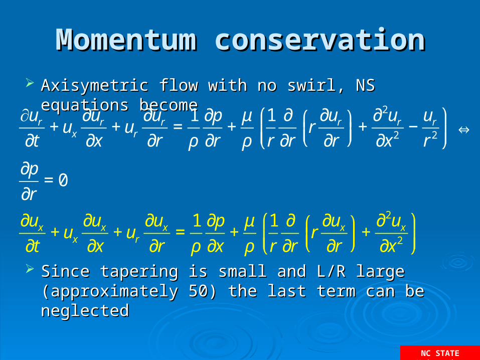
Momentum conservationMomentum conservation Axisymetric flow with no swirl, NS equations becomeAxisymetric flow with no swirl, NS equations become

Since tapering is small and L/R large (approximately 50) Since tapering is small and L/R large (approximately 50) the last term can be neglectedthe last term can be neglected

∂ur

∂t+ ux

∂ur

∂x+ ur

∂ur

∂r=

1

ρ

∂p

∂r+

μ

ρ

1

r

∂

∂rr

∂ur

∂r⎛⎝⎜

⎞⎠⎟

+∂2ur

∂x2−

ur

r2

⎛

⎝⎜⎞

⎠⎟⇔

∂p

∂r= 0

∂ux

∂t+ ux

∂ux

∂x+ ur

∂ux

∂r=

1

ρ

∂p

∂x+

μ

ρ

1

r

∂

∂rr

∂ux

∂r⎛⎝⎜

⎞⎠⎟

+∂2ux

∂x2

⎛

⎝⎜⎞

⎠⎟

NC STATE University

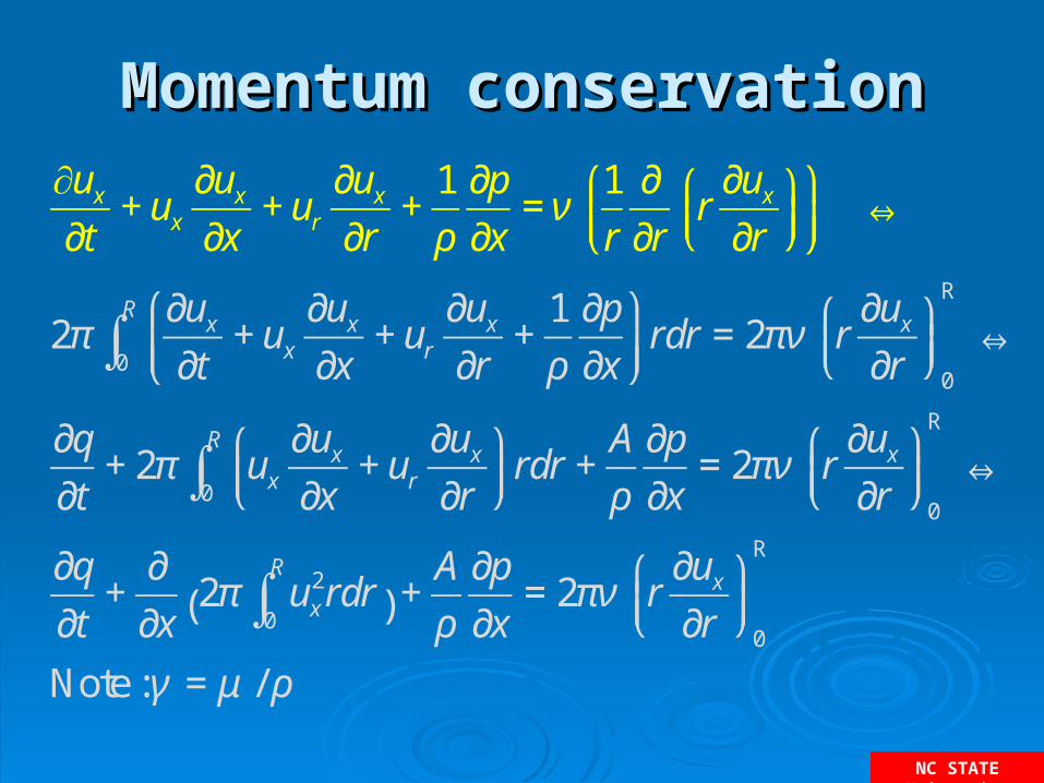
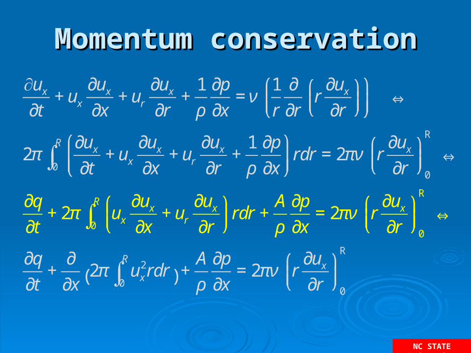
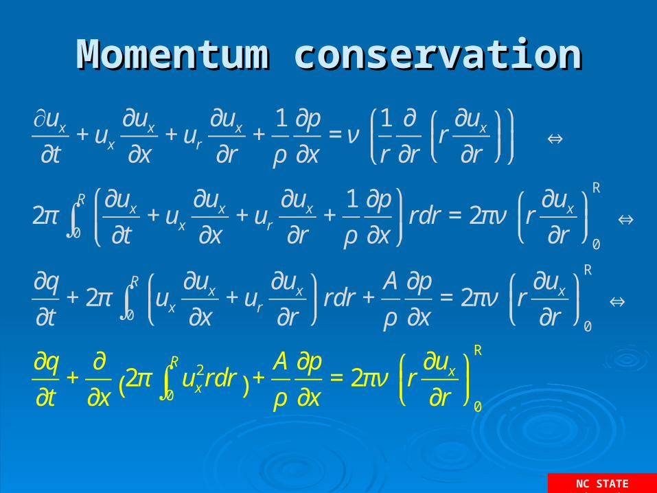
Momentum conservationMomentum conservation∂ux

∂t+ ux

∂ux

∂x+ ur

∂ux

∂r+

1

ρ

∂p

∂x= ν

1

r

∂

∂rr

∂ux

∂r⎛⎝⎜

⎞⎠⎟

⎛⎝⎜

⎞⎠⎟

⇔

2π∂ux

∂t+ ux

∂ux

∂x+ ur

∂ux

∂r+

1

ρ

∂p

∂x

⎛

⎝⎜⎞

⎠⎟rdr = 2πν r

∂ux

∂r⎛⎝⎜

⎞⎠⎟

0

R

⇔0

R

∫

∂q

∂t+ 2π ux

∂ux

∂x+ ur

∂ux

∂r⎛⎝⎜

⎞⎠⎟

rdr +A

ρ

∂p

∂x= 2πν r

∂ux

∂r⎛⎝⎜

⎞⎠⎟

0

R

⇔0

R

∫

∂q

∂t+

∂

∂x2π ux

2rdr0

R

∫( ) +A

ρ

∂p

∂x= 2πν r

∂ux

∂r⎛⎝⎜

⎞⎠⎟

0

R

Note :γ = μ / ρ

NC STATE University

Momentum conservationMomentum conservation

∂ux

∂t+ ux

∂ux

∂x+ ur

∂ux

∂r+

1

ρ

∂p

∂x= ν

1

r

∂

∂rr

∂ux

∂r⎛⎝⎜

⎞⎠⎟

⎛⎝⎜

⎞⎠⎟

⇔

2π∂ux

∂t+ ux

∂ux

∂x+ ur

∂ux

∂r+

1

ρ

∂p

∂x

⎛

⎝⎜⎞

⎠⎟rdr = 2πν r

∂ux

∂r⎛⎝⎜

⎞⎠⎟

0

R

⇔0

R

∫

∂q

∂t+ 2π ux

∂ux

∂x+ ur

∂ux

∂r⎛⎝⎜

⎞⎠⎟

rdr +A

ρ

∂p

∂x= 2πν r

∂ux

∂r⎛⎝⎜

⎞⎠⎟

0

R

⇔0

R

∫

∂q

∂t+

∂

∂x2π ux

2rdr0

R

∫( ) +A

ρ

∂p

∂x= 2πν r

∂ux

∂r⎛⎝⎜

⎞⎠⎟

0

R

NC STATE University

Momentum conservationMomentum conservation

∂ux

∂t+ ux

∂ux

∂x+ ur

∂ux

∂r+

1

ρ

∂p

∂x= ν

1

r

∂

∂rr

∂ux

∂r⎛⎝⎜

⎞⎠⎟

⎛⎝⎜

⎞⎠⎟

⇔

2π∂ux

∂t+ ux

∂ux

∂x+ ur

∂ux

∂r+

1

ρ

∂p

∂x

⎛

⎝⎜⎞

⎠⎟rdr = 2πν r

∂ux

∂r⎛⎝⎜

⎞⎠⎟

0

R

⇔0

R

∫

∂q

∂t+ 2π ux

∂ux

∂x+ ur

∂ux

∂r⎛⎝⎜

⎞⎠⎟

rdr +A

ρ

∂p

∂x= 2πν r

∂ux

∂r⎛⎝⎜

⎞⎠⎟

0

R

⇔0

R

∫

∂q

∂t+

∂

∂x2π ux

2rdr0

R

∫( ) +A

ρ

∂p

∂x= 2πν r

∂ux

∂r⎛⎝⎜

⎞⎠⎟

0

R

NC STATE University

Momentum conservationMomentum conservation

∂ux

∂t+ ux

∂ux

∂x+ ur

∂ux

∂r+

1

ρ

∂p

∂x= ν

1

r

∂

∂rr

∂ux

∂r⎛⎝⎜

⎞⎠⎟

⎛⎝⎜

⎞⎠⎟

⇔

2π∂ux

∂t+ ux

∂ux

∂x+ ur

∂ux

∂r+

1

ρ

∂p

∂x

⎛

⎝⎜⎞

⎠⎟rdr = 2πν r

∂ux

∂r⎛⎝⎜

⎞⎠⎟

0

R

⇔0

R

∫

∂q

∂t+ 2π ux

∂ux

∂x+ ur

∂ux

∂r⎛⎝⎜

⎞⎠⎟

rdr +A

ρ

∂p

∂x= 2πν r

∂ux

∂r⎛⎝⎜

⎞⎠⎟

0

R

⇔0

R

∫

∂q

∂t+

∂

∂x2π ux

2rdr0

R

∫( ) +A

ρ

∂p

∂x= 2πν r

∂ux

∂r⎛⎝⎜

⎞⎠⎟

0

R

NC STATE University

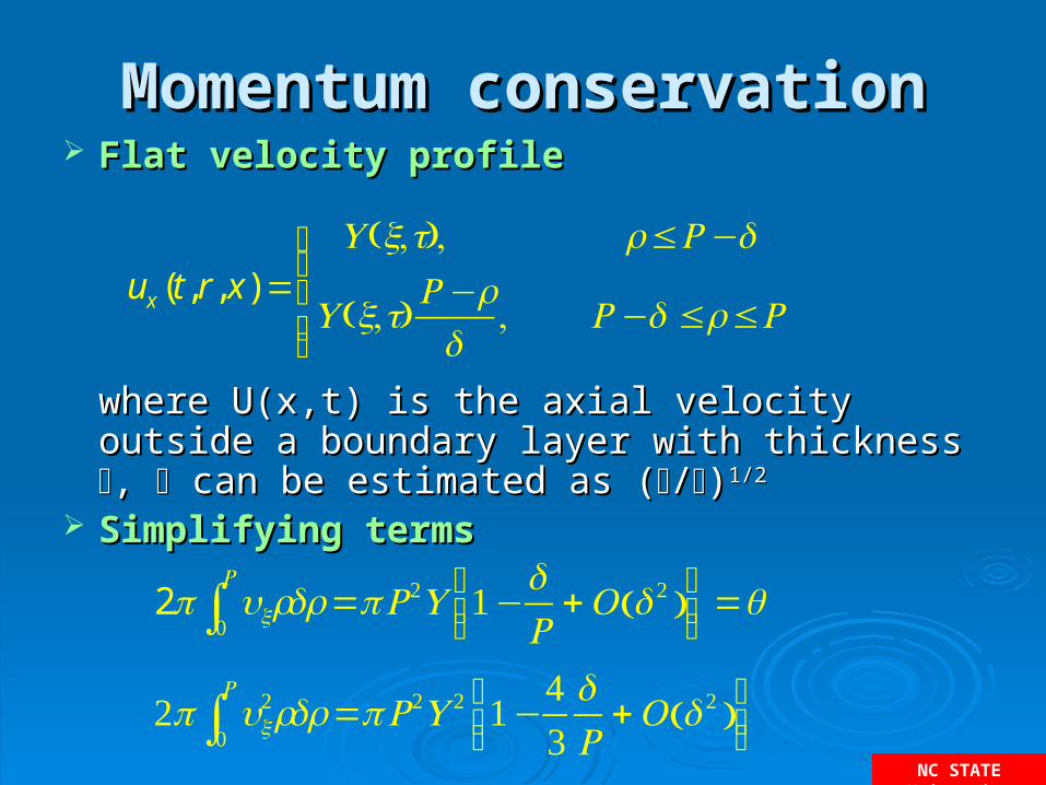
Momentum conservationMomentum conservation Flat velocity profileFlat velocity profile

where U(x,t) is the axial velocity outside a boundary layer where U(x,t) is the axial velocity outside a boundary layer with thickness with thickness , , can be estimated as ( can be estimated as (//))1/21/2

Simplifying termsSimplifying terms

ux (t,r, x) =U(x,t), r ≤R−δ

U(x,t)R−rδ

, R−δ ≤r ≤R

⎧⎨⎪

⎩⎪

2π uxrdr =πR2U 1−δR+O δ 2( )

⎛⎝⎜

⎞⎠⎟0

R

∫ =q

2π ux2rdr =πR2U 2 1−

43δR+O δ 2( )

⎛⎝⎜

⎞⎠⎟0

R

∫

NC STATE University

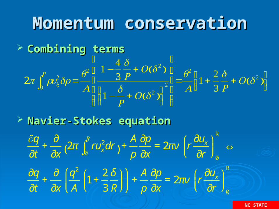
Momentum conservationMomentum conservation Combining termsCombining terms

Navier-Stokes equationNavier-Stokes equation

2π rux2dr =

q2

A

1−43δR+O δ 2( )

1−δR+O δ 2( )

⎛⎝⎜

⎞⎠⎟2

⎛

⎝

⎜⎜⎜⎜

⎞

⎠

⎟⎟⎟⎟

0

R

∫ =q2

A1+

23δR+O δ 2( )

⎛⎝⎜

⎞⎠⎟

∂q

∂t+

∂

∂x2π rux

2dr0

R

∫( ) +A

ρ

∂p

∂x= 2πν r

∂ux

∂r⎛⎝⎜

⎞⎠⎟

0

R

⇔

∂q

∂t+

∂

∂x

q2

A1 +

2

3

δ

R⎛⎝⎜

⎞⎠⎟

⎛

⎝⎜⎞

⎠⎟+

A

ρ

∂p

∂x= 2πν r

∂ux

∂r⎛⎝⎜

⎞⎠⎟

0

R

NC STATE University

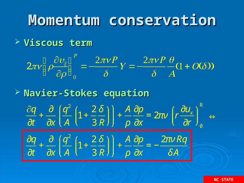
Momentum conservationMomentum conservation Viscous termViscous term

Navier-Stokes equationNavier-Stokes equation

∂q

∂t+

∂

∂x

q2

A1 +

2

3

δ

R⎛⎝⎜

⎞⎠⎟

⎛

⎝⎜⎞

⎠⎟+

A

ρ

∂p

∂x= 2πν r

∂ux

∂r⎛⎝⎜

⎞⎠⎟

0

R

⇔

∂q

∂t+

∂

∂x

q2

A1 +

2

3

δ

R⎛⎝⎜

⎞⎠⎟

⎛

⎝⎜⎞

⎠⎟+

A

ρ

∂p

∂x= −

2πν Rq

δ A

2πν r∂ux∂r

⎛⎝⎜

⎞⎠⎟0

R

=−2πνRδU =−

2πνRδqA

1+O(δ )( )

NC STATE University

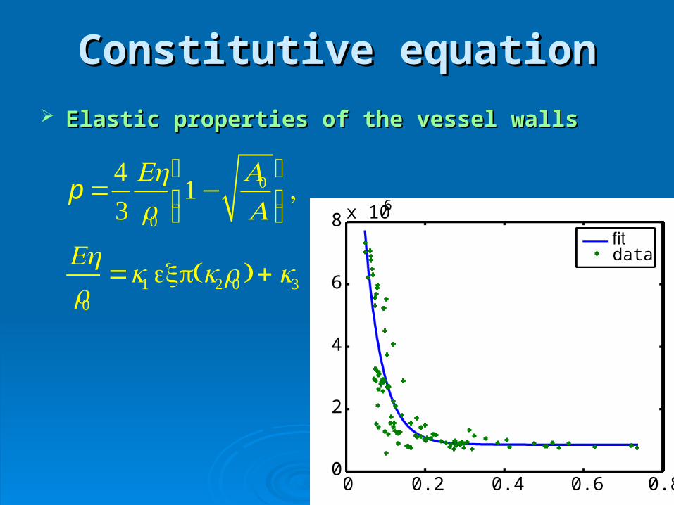
Constitutive equationConstitutive equation Elastic properties of the vessel wallsElastic properties of the vessel walls

p =43Ehr0

1−A0A

⎛

⎝⎜⎞

⎠⎟,

Ehr0

=k1exp(k2r0 ) + k3

0 0.2 0.4 0.6 0.80

2

4

6

8 x 10 6

fitdata

NC STATE University

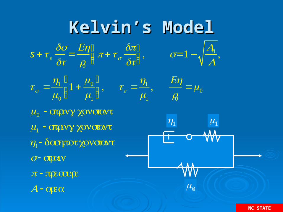
Kelvin’s ModelKelvin’s Model

s +τ εdsdt

=Ehr0p+τσ

dpdt

⎛⎝⎜

⎞⎠⎟, s=1−

A0A,

τσ =η1

0

1+0

1

⎛

⎝⎜⎞

⎠⎟, τ ε =

η1

1

, Ehr0

=0

0 - spring constant1 - spring constantη1- dashpot constants - strain p - pressureA - area

η1 1

0

NC STATE University

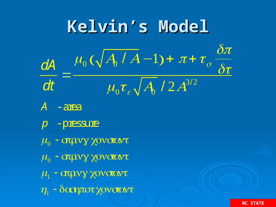
Kelvin’s ModelKelvin’s Model

dA

dt=0 A0 / A−1( ) + p+τσ

dpdt

0τ ε A0 / 2A3/2

A - area

p - pressure

0 - spring constant0 - spring constant1 - spring constantη1 - dashpot constant

NC STATE University

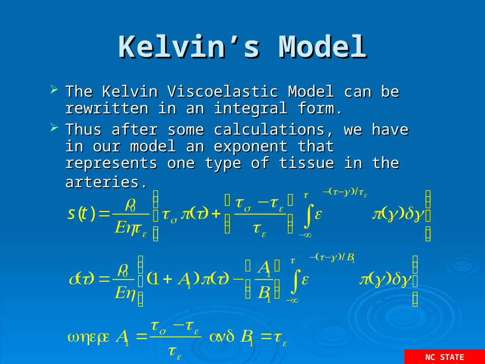
Kelvin’s ModelKelvin’s Model The Kelvin Viscoelastic Model can be The Kelvin Viscoelastic Model can be

rewritten in an integral form.rewritten in an integral form. Thus after some calculations, we have in Thus after some calculations, we have in

our model an exponent that represents one our model an exponent that represents one type of tissue in the arteries.type of tissue in the arteries.

s(t) =r0Ehτ ε

τσ p(t) +τσ −τ ε

τ ε

⎛

⎝⎜⎞

⎠⎟e

−∞

t

∫−(t−γ)/τε

p(γ)dγ⎧⎨⎪

⎩⎪

⎫⎬⎪

⎭⎪

s(t) =r0Eh

(1+ A1)p(t)−A1B1

⎛

⎝⎜⎞

⎠⎟e

−∞

t

∫−(t−γ)/B1

p(γ)dγ⎧⎨⎪

⎩⎪

⎫⎬⎪

⎭⎪

where A1 =τσ −τ ε

τ ε

and B1 =τ ε

NC STATE University

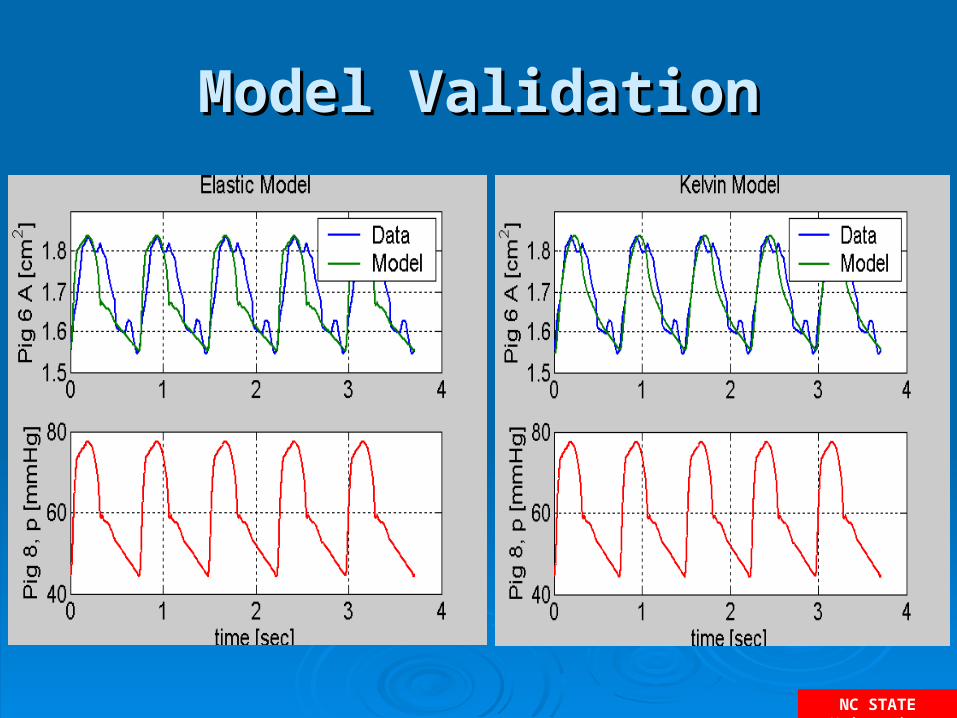
Model ValidationModel Validation

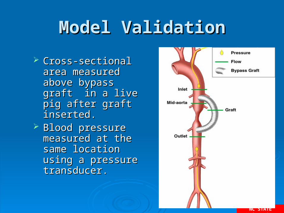
Cross-sectional Cross-sectional area measured area measured above bypass graft above bypass graft in a live pig after in a live pig after graft inserted. graft inserted.

Blood pressure Blood pressure measured at the measured at the same location using same location using a pressure a pressure transducer.transducer.

NC STATE University

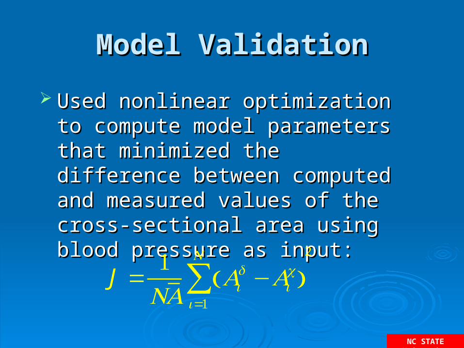
Model ValidationModel Validation

Used nonlinear optimization to Used nonlinear optimization to compute model parameters that compute model parameters that minimized the difference between minimized the difference between computed and measured values of computed and measured values of the cross-sectional area using blood the cross-sectional area using blood pressure as input:pressure as input:

J =1NA

Aid −Ai

c( )i=1

N

∑2

NC STATE University

Model ValidationModel Validation

NC STATE University

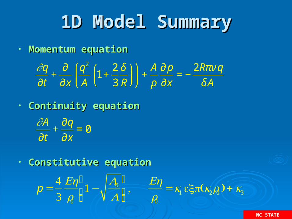
1D Model Summary1D Model Summary• Momentum equationMomentum equation

• Continuity equationContinuity equation

• Constitutive equationConstitutive equation

∂q

∂t+

∂

∂x

q2

A1+

2

3

δ

R⎛⎝⎜

⎞⎠⎟

⎛

⎝⎜⎞

⎠⎟+

A

ρ

∂ p

∂x= −

2Rπν q

δ A

∂A

∂t+

∂q

∂x= 0

p =43Ehr0

1−A0A

⎛

⎝⎜⎞

⎠⎟, Ehr0

=k1exp(k2r0 ) + k3

NC STATE University

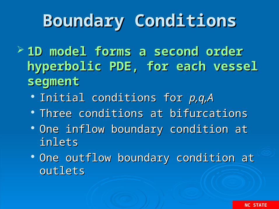
Boundary ConditionsBoundary Conditions

1D model forms a second order hyperbolic PDE, 1D model forms a second order hyperbolic PDE, for each vessel segmentfor each vessel segment Initial conditions for Initial conditions for p,q,Ap,q,A Three conditions at bifurcationsThree conditions at bifurcations One inflow boundary condition at inletsOne inflow boundary condition at inlets One outflow boundary condition at outletsOne outflow boundary condition at outlets

NC STATE University

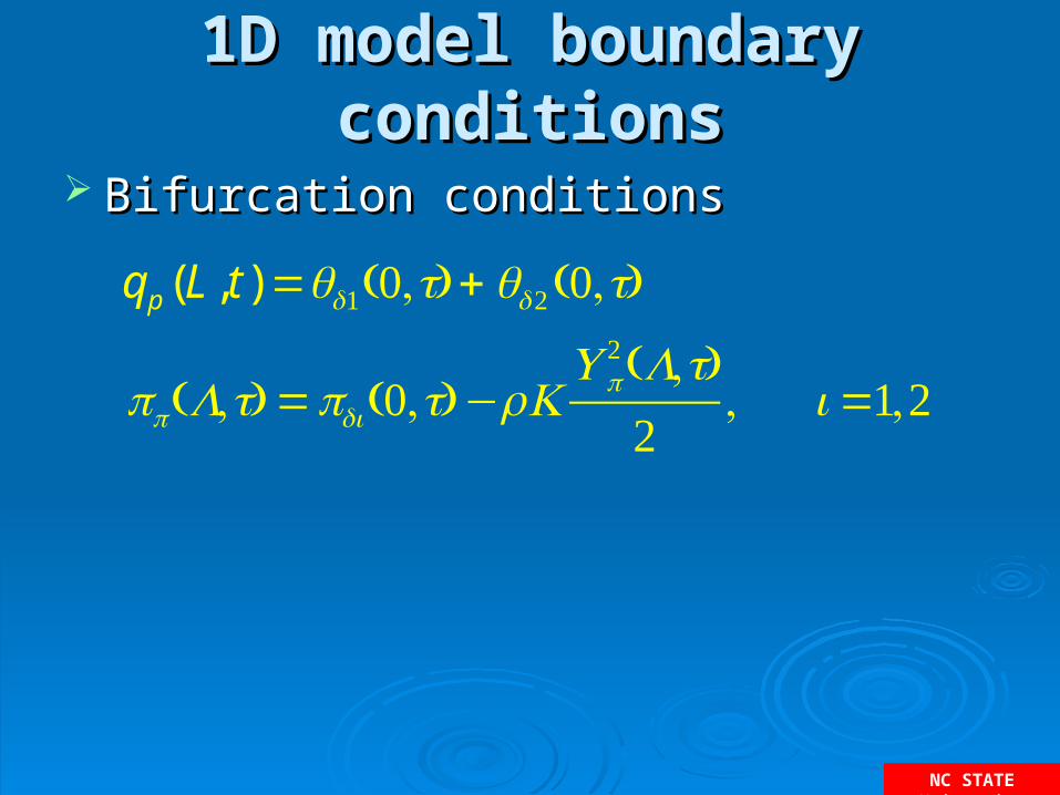
1D model boundary conditions1D model boundary conditions

Bifurcation conditionsBifurcation conditions

qp (L,t) =qd1(0,t) +qd2 (0,t)

pp(L,t) =pdi (0,t)−ρKUp

2 (L,t)2

, i =1,2

NC STATE University

1D model boundary conditions1D model boundary conditions

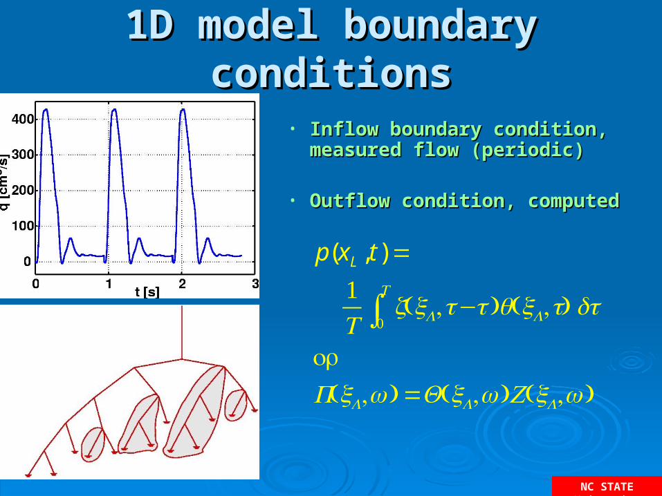
• Inflow boundary condition, Inflow boundary condition, measured flow (periodic)measured flow (periodic)

• Outflow condition, computedOutflow condition, computed

p(xL , t) =

1T

z(xL ,t−τ)q(xL ,t) dτ0

T

∫or

P(xL ,ω ) =Q(xL ,ω )Z(xL ,ω )

NC STATE University

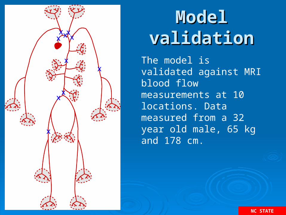
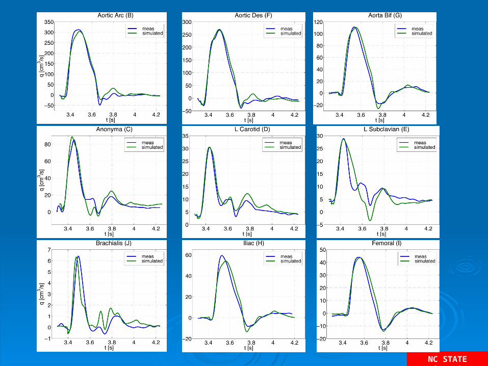
Model validationModel validation

The model is validated against MRI blood flow measurements at 10 locations. Data measured from a 32 year old male, 65 kg and 178 cm.

NC STATE University

NC STATE University

ReferencesReferences Chorin and Marsden: A Mathematical Introduction to Chorin and Marsden: A Mathematical Introduction to

Fluid Mechanics, 3rd edition, Springer Verlag, 2000Fluid Mechanics, 3rd edition, Springer Verlag, 2000 Aceheson: Elementary Fluid Dynamics, Oxford Aceheson: Elementary Fluid Dynamics, Oxford

University Press, 1990University Press, 1990 Lighthill: Mathematical Biofluiddynamics, CBMS-NSF Lighthill: Mathematical Biofluiddynamics, CBMS-NSF

Regional Conference Series in Applied Mathematics, Regional Conference Series in Applied Mathematics, 19831983

Fung: Biomecanics - Circulation, Sprigner Verlag, 1996Fung: Biomecanics - Circulation, Sprigner Verlag, 1996 Fung: Biomechanics - Mechanical Properties of Living Fung: Biomechanics - Mechanical Properties of Living

Tissue, Springer Verlag, 1993Tissue, Springer Verlag, 1993 Ottesen, Olufsen, Larsen: Mathematical Models in Ottesen, Olufsen, Larsen: Mathematical Models in

Human Physiology, SIAM, 2004 (Book)Human Physiology, SIAM, 2004 (Book)

NC STATE University

Postural change: sit-to-standPostural change: sit-to-stand

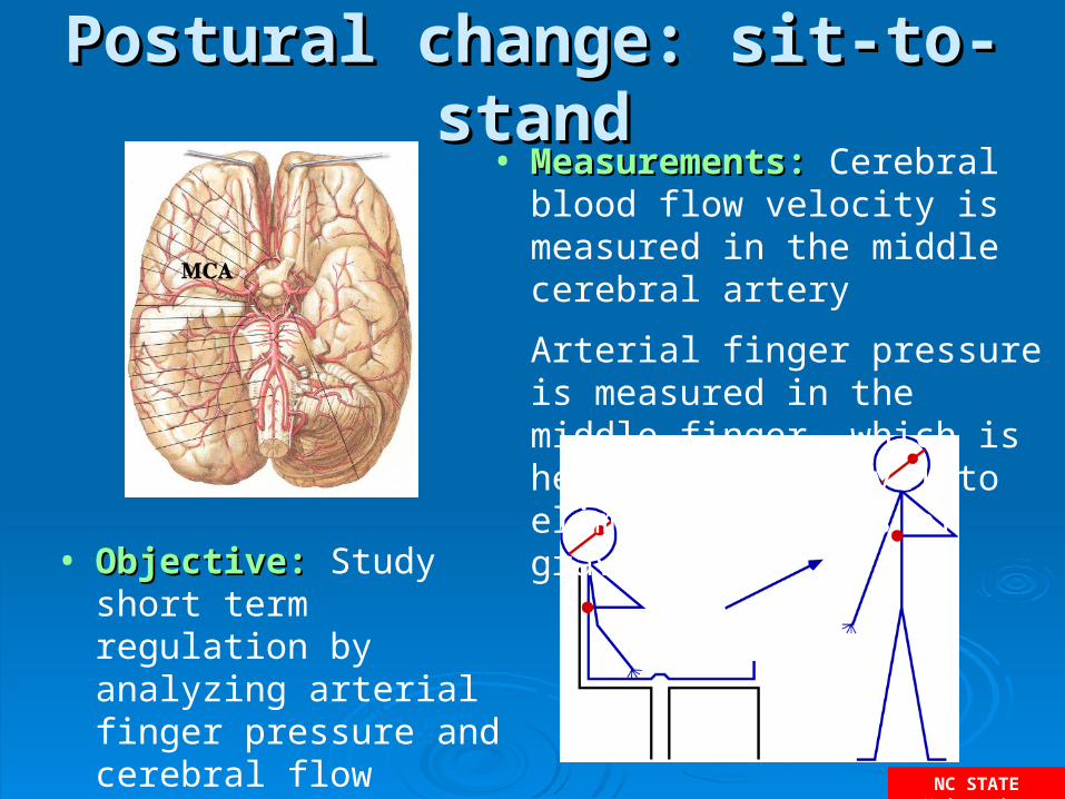
• Objective:Objective: Study short term regulation by analyzing arterial finger pressure and cerebral flow velocity during postural change from sitting to standing

• Measurements: Measurements: Cerebral blood flow velocity is measured in the middle cerebral artery

Arterial finger pressure is measured in the middle finger, which is held at heart level to eliminate effects of gravity

NC STATE University

Effects of postural changeEffects of postural change

• Approximately 500 cc of blood is pooled in lower extremities as a result of gravitational force

• Venous return is reduced leading to a decrease in stroke volume

• Arterial blood pressure in the trunk and upper extremities drop, while blood pressure in the lower extremities is increased

• Blood flow to the brain is reduced leading to build up of CO2

NC STATE University

Autonomic regulationAutonomic regulation Autonomic baroreflexes, mediated by CNS restoreheart rate, arterial BP, and cerebral BF. Sympathetic response: Increased sympathetic activity increases

release of noradrenaline, which increases heart rate, cardiac contractility, vascular resistance, compliance (6-8 cardiac cycles).

Parasympathetic response: Decreased parasympathetic activity decreases release of ach, which increases heart rate and cardiac contractility (1-2 cardiac cycles).

Cholinergic response: Parasympathetic release of ach in the brain may lead to a decrease of cerebrovascular resistance.

NC STATE University

Cerebral autoregulationCerebral autoregulation

Cerebral autoregulationCerebral autoregulation maintain cerebral perfusion.maintain cerebral perfusion. Myogenic control:Myogenic control: A decrease in pressure relaxes muscles in the A decrease in pressure relaxes muscles in the

vessel wall, which makes vessels dilate to maintain cerebral vessel wall, which makes vessels dilate to maintain cerebral perfusion.perfusion.

Oxygen demand control:Oxygen demand control: A decrease in cerebral perfusion A decrease in cerebral perfusion increases COincreases CO2 2 and decreases metabolites related to O and decreases metabolites related to O22 supply. To supply. To maintain cerebral perfusion cerebrovascular resistance is decreasedmaintain cerebral perfusion cerebrovascular resistance is decreased..

NC STATE University

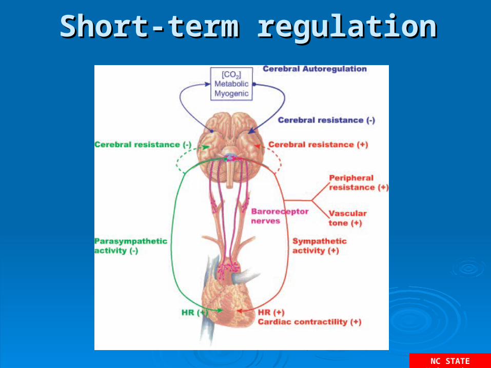
Short-term regulationShort-term regulation

NC STATE University

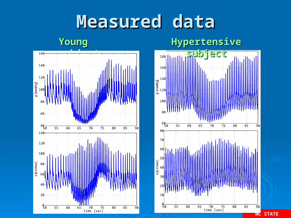
Measured dataMeasured dataYoung subjectYoung subject

50 55 60 65 70 75 80 85 9040

60

80

100

120

140

160

time [sec]

50 55 60 65 70 75 80 85 900

20

40

60

80

100

120

140

time [sec]

50 55 60 65 70 75 80 85 9060

80

100

120

140

160

180

time [sec]

Hypertensive subjectHypertensive subject

50 55 60 65 70 75 80 85 900

10

20

30

40

50

60

70

80

time [sec]

NC STATE University

Modeling objectiveModeling objective

• Develop mathematical models to:Develop mathematical models to:

– Understand how postural change alters cerebral and systemic vascular resistances, compliance, heart rate, and cardiac contractility

– Study how these factors change in young, healthy elderly, and hypertensive elderly subjects