Embed Size (px)
Citation preview

Modeling and Simulation of RLC Networks & Modal Equivalents for Transmission Networks Containing
Distributed Parameter Lines
1
Model Based Systems Engineering (MBSE) Lecture Series
N. Martins Talk - Part 2
Sergio L. Varricchio, CEPEL and multiple co-authors*
(*) Sergio Gomes Jr. (CEPEL), Nelson Martins (CEPEL), Francisco D. Freitas (University of Brasilia), Carlos M. Portela (COPPE), Leonardo Lima (Kestrel Power), Franklin C. Veliz (CEPEL)
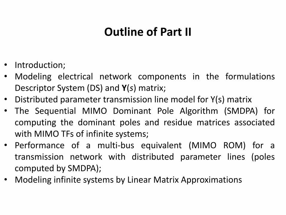
• Introduction; • Modeling electrical network components in the formulations
Descriptor System (DS) and Y(s) matrix; • Distributed parameter transmission line model for Y(s) matrix • The Sequential MIMO Dominant Pole Algorithm (SMDPA) for
computing the dominant poles and residue matrices associated with MIMO TFs of infinite systems;
• Performance of a multi-bus equivalent (MIMO ROM) for a transmission network with distributed parameter lines (poles computed by SMDPA);
• Modeling infinite systems by Linear Matrix Approximations
Outline of Part II

• Modal Analysis – Involves the calculation of the system matrix, its poles & zeros
and their sensitivities to system parameters;
– Provides system structural information: mode shapes, participation factors, TF dominant poles, reduced order models;
– Matrix models are used for the study of different power system phenomena:
• Eletromechanical transients
• Subsynchronous resonance
• Harmonic performance; • Electromagnetic Transients.
(High-frequency network modeling, all transmission lines having distributed parameters)
Introduction to Part II (1/2)
(Lumped R-L-C dynamic network modeling);
(Algebraic network modeling, R+jX);

• High Frequency Modeling of Electrical Networks
– 3 formulations: State Space (SS), Descriptor Systems (DS) and Y(s) matrix;
– The distributed parameter nature of transmission lines (TL) can be modeled by transcendental functions having infinite poles – Infinite systems;
– Infinite systems are neatly modeled by the Y(s) matrix formulation;
– Finite approximations of infinite systems can be modeled in the SS and DS formulations, where TLs are represented by cascaded RLC circuits;
– Various NLA methods exist to efficiently compute ROMs for large scale DS models;
– A main disadvantage of the Y(s) matrix formulation is the inexistance of robust and efficient algorithms for the computation of the poles and residue matrices of multivariable TFs.
Introduction to Part II (2/2)

• Basic equations:
ttt uBxAxT
ttt TuDxCy
• The components of the system are described by first-order ordinary differential equations and algebraic equations as well;
• The Kirchhoff Law of Currents for each individual node of the network is then added to these equations, to define the connection among the various existing system components;
• The DS model is a generalization of the SS model and leads to a simpler and more efficient computer implementation.
Descriptor Systems (1/5)

DBATCH 1
ss T
Transfer Functions
TF SISO
dssu
sysH T
bATc
1
djjH T
bATc1
TF MIMO
Frequency Response
tttt
ttt
t
uuBxATxAT
22
tttttt T uDxCy
Time Response (trapezoidal rule of integration)
Descriptor Systems (2/5)

jkkjC
kjvviRv
dt
diL
kjC i
dt
dvC
R
L
C
ikj
vC
iLvk vj
k jvC
R L C
vk ikj vj
k j
RLC Parallel Voltage Source RLC Series
fjkff
f
f vvviRdt
diL
jRf Lf
k
ifvk vjvf
CL v
dt
diL
kjCLC iv
Ri
dt
dvC
1
0 Cjk vvv
Kirchhoff Current Law
Node k 0m
mki
→ Nodes connected to k
→
Descriptor Systems (3/5)

L12
R12
L13
R13
C3 R3 L3
C1 L1
C2 R2 L2v2 2Li
barra 1
barra 2 barra 3
Parameters for 3-bus system
Input → i2 = 1 pu
Output → v1 (pu)
v1 Ind. (mH) Res. () Cap. (F)
L1 8.0 R2 80.0 C1 23.9
L2 424.0 R3 133.0 C2 8.0
L3 531.0 R12 0.46 C3 11.9
L12 9.7 R13 0.55
L13 11.9
i2
Nominal Frequency: 50 Hz Nominal Voltage: 20 kV MVA base: 10 MVA
Descriptor Systems (4/5) Matlab script vs PSCAD Validation
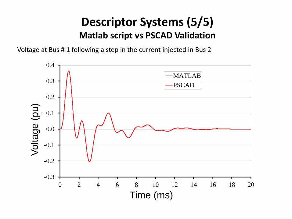
Voltage at Bus # 1 following a step in the current injected in Bus 2
-0.3
-0.2
-0.1
0.0
0.1
0.2
0.3
0.4
0 2 4 6 8 10 12 14 16 18 20
Ten
são
(p
u)
Tempo (ms)
MATLAB
PSCAD
Voltage (
pu
)
Time (ms)
Descriptor Systems (5/5) Matlab script vs PSCAD Validation

130 21220 iii
3
2
3
2
1
13
12
30
20
10
13
12
3
2
1
1
1
11
11
1111
1
11
11
11
111
1
11
111
1
11
1
3
3
2
2
1
i
i
v
v
v
v
i
i
i
i
v
i
i
v
i
i
v
R
R
R
R
R
f
f
C
L
C
L
C
f
3
2
1
13
12
30
20
10
13
12
3
3
2
2
1
3
3
2
2
1
v
v
v
i
i
i
i
v
i
i
v
i
i
v
dt
d
L
L
L
C
L
C
L
C
f
C
L
C
L
C
f
71
30
3
3 33
3 ivR
idt
dvC CL
C
(7)
(7)
(13)
(13)
3
2
3
2
1
13
12
30
3
3
20
2
2
10
1
3
2
1
1
1
1
i
i
v
v
v
v
i
i
i
i
v
i
i
v
i
i
v
v
v
v f
f
C
L
C
L
C
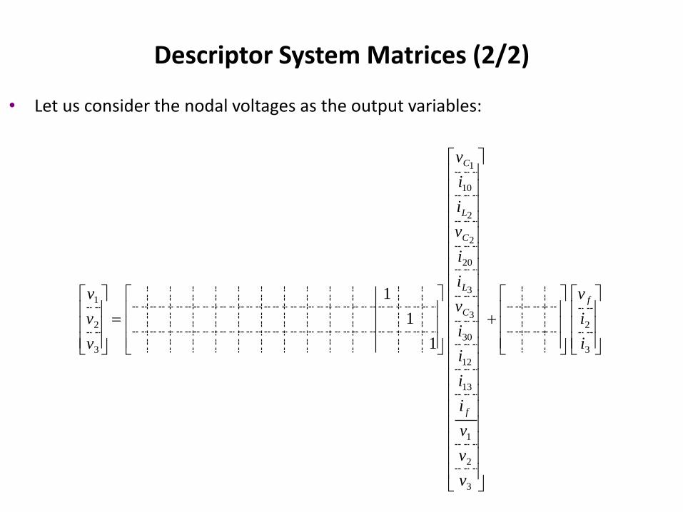
Descriptor System Matrices (2/2)
• Let us consider the nodal voltages as the output variables:

• Basic equations:
sss uBxY
sss TuDxCy
• Elements
• Diagonal yii: Summation of the all elementary admittances connected to node i;
• Off-diagonal yij: negative value of summation of all elementary admittances connected between nodes i and j;
• SS and DS formulations are particular cases of Y(s): Y(s) = (sT – A)
• Voltage sources are modeled by additional equations;
• The derivative of Y(s) with respect to s, for the computation of the system poles, is automatically built by coding simple rules that are similar to those used for building Y(s).
Y(s) Matrix Formulation

Transfer Function
SISO TF
MIMO TF DBYCH 1
ss T
dssu
sysH T
bYc
1
djjH T
bYc1
Frequency Response
Y(s) Matrix Formulation

Parallel RLC Voltage Source Series RLC
R L Ck j
R
L
C
k j k kfi
kfv
kfR
kfL
CsLsR
yseries 1
1
2
2
1
1
CsLsR
CsL
ds
dyseries
sCsLR
yparallel 11
LsC
ds
dyparallel
2
1
01
kf
n
j
jkj ivy
kkk fffk vizv
kkk fff LsRz
k
k
f
fL
ds
dz
where:
Y(s) Matrix Formulation – Basic Elements
13131212
111
11
LsRLsRCsy
L12
R12
L13
i13
R13
i3i2
i12
i20
C3 R3 L3v3
i30
C1v1
i10
3LiC2 R2 L2v2 2Li
barra 1
barra 2 barra 3
Rf
Lf
if
vf
fff
v
i
i
i
v
v
v
z
yy
yy
yyy
3
2
3
2
1
3331
2221
131211
100
010
001
000
001
00
00
1
sY
Voltage Source
1313
3113
1
LsRyy
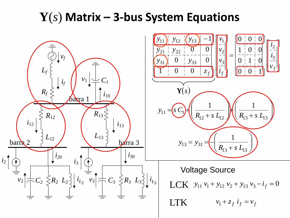
LCK 0313212111 fivyvyvy
LTK fff vizv 1
Y(s) Matrix – 3-bus System Equations

21313
133113
LsR
L
ds
dy
ds
dy
21313
132
1212
121
11
LsR
L
LsR
LC
ds
dy
dsdz
dsdydsdy
dsdydsdy
dsdydsdydsdy
ds
sd
f000
00
00
0
3331
2221
131211
Y
L12
R12
L13
i13
R13
i3i2
i12
i20
C3 R3 L3v3
i30
C1v1
i10
3LiC2 R2 L2v2 2Li
barra 1
barra 2 barra 3
Rf
Lf
if
vf
Fonte de Tensão
f
fffL
ds
LsRd
ds
dz
Y(s) Matrix – 3-bus System Equations

L12
R12
L13
i13
R13
i3i2
i12
i20
C3 R3 L3v3
i30
C1v1
i10
3LiC2 R2 L2v2 2Li
barra 1
barra 2 barra 3
Rf
Lf
if
vf
fff
v
i
i
i
v
v
v
z
yy
yy
yyy
3
2
3
2
1
3331
2221
131211
100
010
001
000
001
00
00
1
ff
v
i
i
i
v
v
v
v
v
v
3
2
3
2
1
3
2
1
000
000
000
0100
0010
0001
A compact description
sss uDxCy
MIMO System
sss uBxY
sss uDxCy
Y(s) Matrix – 3-bus System Equations

DS compared to Y(s) Matrix:
Transfer Impedance between
buses 1 & 2
0.0
0.2
0.4
0.6
0.8
1.0
1.2
1.4
0 250 500 750 1000 1250 1500
|z12| (
pu
)
Frequência (Hz)
Sistema Descritor
Matriz Y(s)
-200
-100
0
100
200
0 250 500 750 1000 1250 1500
Fas
e(z 1
2) (g
rau
s)
Frequência (Hz)
Sistema Descritor
Matriz Y(s)
Y(s) matrix- Freq. response results for 3-bus system
Matriz Y(s) – Modelagem de Redes
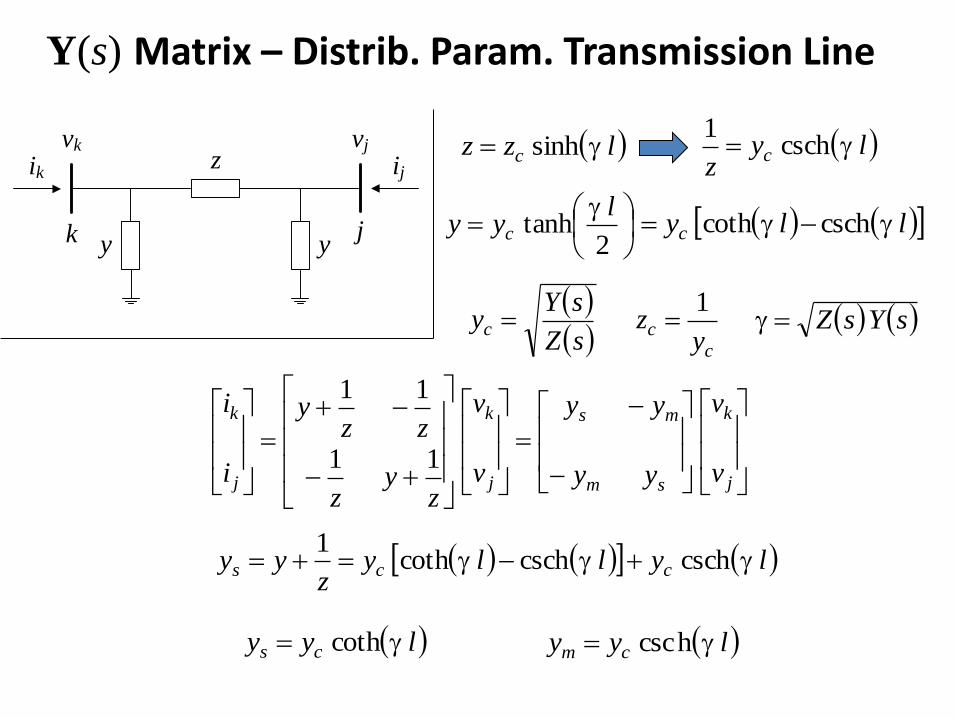
z
yyk
vk
j
vj
ik ij
lzz c sinh
lyz
c csch1
llyc cschcoth
sZ
sYyc
c
cy
z1
sYsZ
j
k
sm
ms
j
k
j
k
v
v
yy
yy
v
v
zy
z
zzy
i
i
11
11
lylly
zyy ccs cschcschcoth
1
lyy cs coth lyy cm hcsc
2tanh
lyy c
Y(s) Matrix – Distrib. Param. Transmission Line

Matriz Y(s) – Modelagem de Redes
lyy cs coth
lyy cm hcsc
sZ
sYyc
sYsZ
llds
dyl
ds
dy
ds
dyc
cs csch coth
lllds
dyl
ds
dy
ds
dyc
cm coth csch csch
ds
dZy
ds
dY
ds
dyc
c 2
2
1
2
1
ds
dZY
ds
dYZ
ds
d
Y(s) Matrix – Distrib. Param. Transmission Line

Matriz Y(s) – Modelagem de Redes
1CsY 1Cds
dY
gie ZZZZ
ds
dZ
ds
dZ
ds
dZ
ds
dZ gie
ee LsZ 1
ee
Lds
dZ1
Positive sequence capacitance & indutance, computed by
matrix reduction considering ideal conductor and soil.
eLC 11,
Y(s) Matrix – Distrib. Param. Transmission Line

Matriz Y(s) – Modelagem de Redes
sm
sn
n
skZ
s
i
x
y
Condutor
Aço
ri re
er
ssk
2
1
10010110 KIKIsn
11010111 KIKIsm
sri0 sre1
I0, I1 → Modified Bessel functions of first kind for integer orders 0 & 1,
respectively.
K0, K1 → Modified Bessel functions of first kind for integer orders 0 & 1,
respectively.
Y(s) Matrix – Distrib. Param. Transmission Line

Matriz Y(s) – Modelagem de Redes
2
1
sm
ds
sdmsn
ds
sdnsm
sksm
sn
ds
sdk
nds
dZ
s
i
s
sk
ds
sdk
2
ds
d
d
dKIK
ds
d
d
dI
ds
d
d
dKIK
ds
d
d
dI
ds
sdn 1
1
100110
0
0
010
0
011001
1
1
10
sd
d
d
dKIK
ds
d
d
dI
sd
d
d
dKIK
sd
d
d
dI
ds
sdm 1
1
110111
0
0
010
0
011101
1
1
11
sds
d
2
00
sds
d
2
11
1
0 Id
dI
2
201
II
d
dI
1
0 Kd
dK
2
201
KK
d
dK
sm
sn
n
skZ
s
i
Y(s) Matrix – Distrib. Param. Transmission Line

Matriz Y(s) – Modelagem de Redes
x
y
D12
H1
1
2
3
3
1
3
122
223
1
02
lnln6
iij
j ijji
ijji
i i
ig
DHH
DpHH
H
pHsZ
3
1
3
122
3
1
0ˆ
ˆ
ˆlnln
6i
ijj
ij
ijijji
ij
i ii
ig
ds
pHd
pH
s
DHH
H
ds
dp
pH
s
H
pH
ds
dZ
ssp
1
222ˆ
ijjiij DpHHH
2
2 3ps
ds
dp
ds
dp
DpHH
pHH
ds
pHd
ijji
jiij
222
22ˆ
Y(s) Matrix – Distrib. Param. Transmission Line

vf
1 2Rf Z
Y Y
R3
L3
C3
3Lf L12
dsdz
dsdydsdy
dsdydsdydsdy
dsdydsdy
ds
sd
f000
00
0
00
3332
232221
1211
Y
25
Z
YCsLsR
sy11
3
33
33
lssy
ds
dC
LsR
L
ds
dyc
coth32
123
333
lssyc coth
fz
yy
yyy
yy
s
001
00
0
10
3332
232221
1211
Y
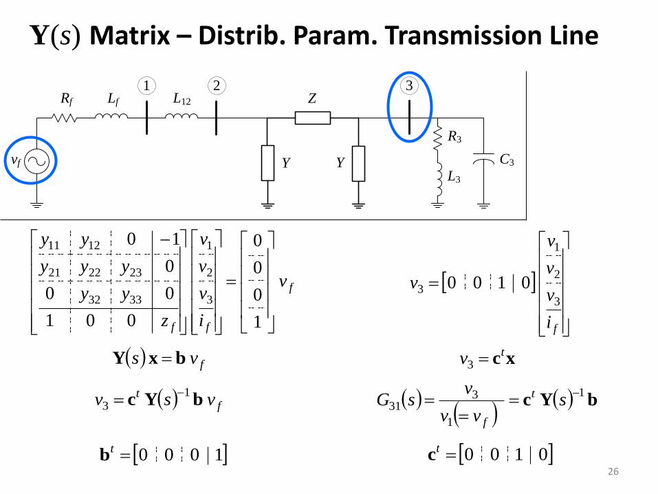
Y(s) Matrix – Distrib. Param. Transmission Line
vf
1 2Rf Z
Y Y
R3
L3
C3
3Lf L12
26
f
ff
v
i
v
v
v
z
yy
yyy
yy
1
0
0
0
001
00
0
10
3
2
1
3332
232221
1211
0100tc
fi
v
v
v
v3
2
1
3 0100
1000tb
fvs bxY xctv 3
ft vsv bYc
13
bYc
1
1
331
s
vv
vsG t
f
Y(s) Matrix – Distrib. Param. Transmission Line

Sequential MIMO Dominant Pole Algorithm
(SMDPA)

DBYCH 1
ss T eT ss DBYCH
1
Direct Matrix
iD
ei DDD
ds
sd
s
HK
lim
es
i ss DKHD
lim
ei
i i
i ss
s DDKR
H
1
Partial Fraction Expansion
SMDPA – Fundamental Concepts (1/3)

DKHH sssˆ
kii ik
i
k
kk
jj
1
ˆ RRH
Strictly Proper part of H(s)
DKR
H
ss
si i
i
1
The pole k will be dominant in H(s) if the magnitude of ( ||Rk||2 / |k| )
is sufficiently large so as to cause a peak in the plot of max[Ĥ(j)] in
the close neighborhood of the frequency k.
Let k = k + j k be a pole with an associated residue matrix Rk, then:
Dominant Pole
SMDPA – Fundamental Concepts (2/3)
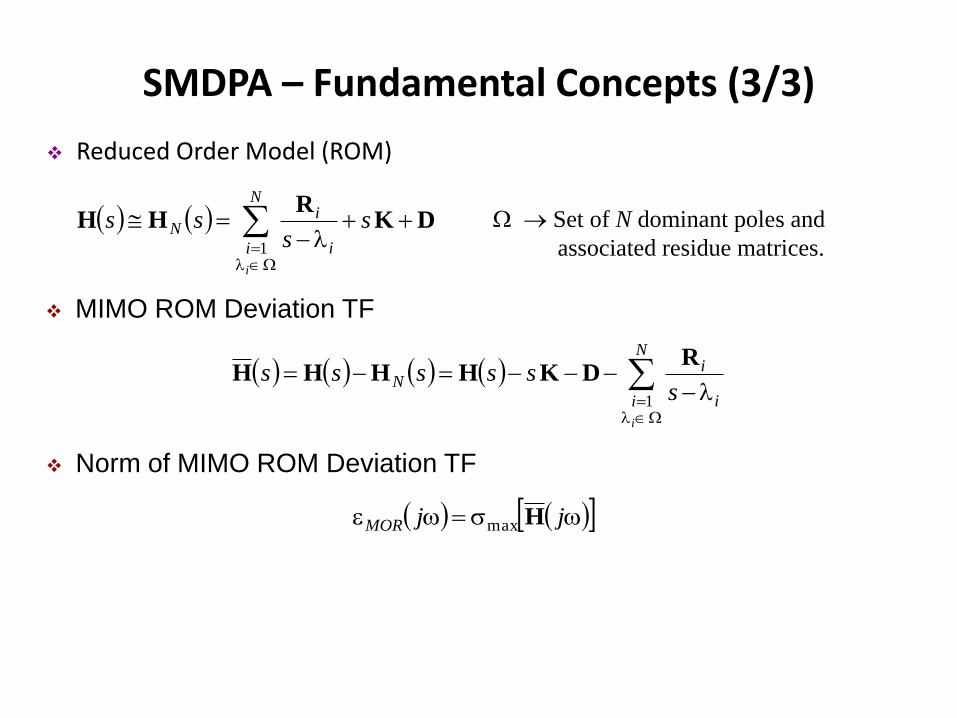
Reduced Order Model (ROM)
Set of N dominant poles and
associated residue matrices.
DKR
HH
ss
ssN
i i
iN
i
1
N
i i
iN
i
ssssss
1
RDKHHHH
jjMOR Hmax
MIMO ROM Deviation TF
Norm of MIMO ROM Deviation TF
SMDPA – Fundamental Concepts (3/3)

The set of dominant poles of H(s) may be efficiently computed only when eliminating from H(s):
• The N previously computed poles (deflation);
• Matrices K and D.
The Newton method should therefore be applied to the MIMO ROM deviation TF:
N
i i
i
i
ssss
1
RDKHH
SMDPA – Newton Method (1/3)

0lim1
min
s
sH
0min ssf
Newton equationing
kk
kk
k
sds
sdss
s
min
*
minmin
)(
1
vH
w
ds
sd
ds
sd
ds
sd NHHH
N
i i
iN
i
sds
sd
12
KRH
BXY B ss
CXY C ssT
s
ds
sds
ds
sd TBC X
YX
H
sss kk 1
vmin, wmin eigenvectors associated with min.
The sparse solution of these two matrix equations sistemas require a single LU factorization and various solves.
mim minimum eigenvalue of 1sH
Pole of
sH
mim, vmin, wmin)
function eig of Matlab.
SMDPA – Newton Method (2/3)

0.1
1.0
10.0
1000 1500
m
ax[Ĥ
(j
)] (
pu
)
Frequência (Hz)
0.1
1.0
10.0
1000 1500
m
ax[Ĥ
(j
)] (
pu
)
Frequência (Hz)
Determining the initial pole estimates
f1 f2 f3 f4 f5 f6 f7
810 2 ffj s
f8
SMDPA – Newton Method (3/3)

Computation of the Residue Matrix for a Pole
Definition of the Integration Curve
j
Real(s)
4
1
1
k
P
PC
dssdss
k
k
HH
P2 P1
P3 P4
j
Real(s)
≡ P5
C
dssj C
HR2
1
SMDPA – Pole Residue Matrix (1/2)

kkk PlPPl 15.0,, HJ
Legendre-Gauss Method with Error Control
kP kk PP kk PP 2 kk PlP 1 kk PlP kkk PmP 1 kkk PmP 1 1kP
kk PlPs 15.0
4
1 1 1k
m
l
PlP
PlPC
k kk
kk
dssdss HH
4
1 1 1
,,2
k
m
l
M
i
kiik
k
PlwP
J
4
1 1 1
,,22
1
k
m
l
M
i
kiik
k
PlwP
jJR ,,,
22
1
1 1
km
l
M
i
kiik
k PlwP
jJR 4,,1 k
,2,1,0,2 qm qk
2
1
2
1 qk
qk
qkk RRR max
4
1
4 k
k
• Determining the Error
SMDPA – Pole Residue Matrix (2/2)

The 34-bus test system with 25 distributed parameter TLs
241312
26
27 34 11
287
8
29
9
32
25
21
20
23 33
22 31
30106
1 2 34 5
18 19
17
14 15 16
Element Quant.
Buses 34
TLs 25
Branches 12
Trafos 16
Loads 16
Generators 10
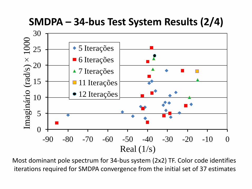
SMDPA – 34-bus Test System Results (1/4)
0
5
10
15
20
25
30
-90 -80 -70 -60 -50 -40 -30 -20 -10 0
Imag
inár
io (
rad/s
)
10
00
Real (1/s)
5 Iterações
6 Iterações
7 Iterações
11 Iterações
12 Iterações
Most dominant pole spectrum for 34-bus system (2x2) TF. Color code identifies iterations required for SMDPA convergence from the initial set of 37 estimates
SMDPA – 34-bus Test System Results (2/4)

0.0
1.0
2.0
3.0
4.0
0 500 1000 1500 2000 2500 3000 3500 4000
m
ax(p
u)
Frequência (Hz)
SMDPA – 34-bus Test System Results (3/4)
0.0
1.0
2.0
3.0
4.0
0 500 1000 1500 2000 2500 3000 3500 4000
m
ax(p
u)
Frequência (Hz)
Infinite
ROM 151

1.0E-05
1.0E-04
1.0E-03
1.0E-02
0 1000 2000 3000 4000
MO
R(p
u)
Frequência (Hz)
SMDPA – 34-bus Test System Results (4/4)
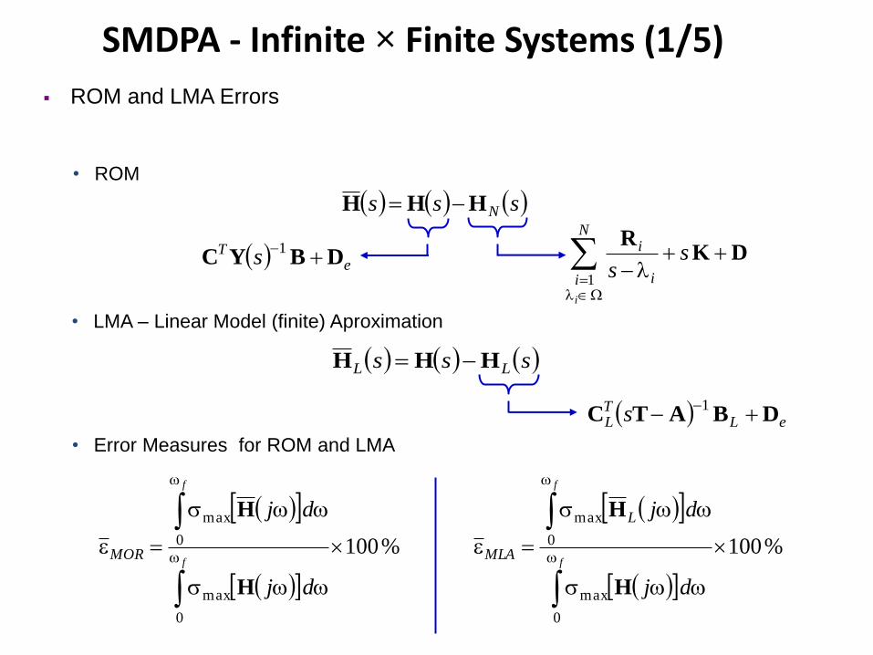
ROM and LMA Errors
sss NHHH
DKR
ss
N
i i
i
i
1
eT s DBYC
1
sss LL HHH
• ROM
• LMA – Linear Model (finite) Aproximation
eLTL s DBATC
1
%100
0
max
0
max
f
f
dj
dj
MOR
H
H
• Error Measures for ROM and LMA
%100
0
max
0
max
f
f
dj
djL
MLA
H
H
SMDPA - Infinite × Finite Systems (1/5)

How many circuits to use in the TL models of the 34-bus system?
The tables below compare the performances of finer LMAs ROM-151
n nD nL nL n
300 15063 15182 345.05
400 20063 20182 458.68
500 25063 25182 572.32
600 30063 30182 685.95
Statistics for LMA models
n Number of circuits per TL
nD Number of differencial equations
nL Dimension of matrices A and T
n Dimension of matrix Y(s) ( no of buses + no of voltage sources 44)
n MLA (%) MOR (%)
300 4.59 × 101
400 2.58 × 101
1.94 × 10
1
500 1.65 × 101
600 1.15 × 101
Error Measures for LMA and ROM
SMDPA - Infinite × Finite Systems (2/5)

1.0E-05
1.0E-04
1.0E-03
1.0E-02
1.0E-01
1.0E+00
0 2000 4000 6000 8000
MO
R(p
u)
Frequência (Hz)
1.0E-05
1.0E-04
1.0E-03
1.0E-02
1.0E-01
1.0E+00
0 2000 4000 6000 8000
MO
R(p
u)
Frequência (Hz)
Simple procedure for improving ROM Fidelity of infinite systems
• ROM – 151 for MIMO TF of 34-bus system
These eight spikes are due to the 8 pairs of poles that are dominant in the adjacent 4 - 8 KHz region, and cause the error curve within the 0 – 4 KHz window to rise.
Frequency Range of
Interest
SMDPA - Infinite × Finite Systems (3/5)

1.0E-05
1.0E-04
1.0E-03
1.0E-02
0 1000 2000 3000 4000
MO
R(p
u)
Frequência (Hz)
1.0E-05
1.0E-04
1.0E-03
1.0E-02
0 1000 2000 3000 4000
MO
R(p
u)
Frequência (Hz)
Assessing ROM Fidelity for the MIMO TF of 34-bus System
• ROM - 151 ROM - 167
ROM 151
ROM 167
SMDPA - Infinite × Finite Systems (4/5)

(300, 0.459)
(400, 0.258)
(500, 0.165)
(600, 0.115)
0.0
0.1
0.2
0.3
0.4
0.5
100 200 300 400 500 600 700
Err
o (
%)
Número de s
(300, 0.459)
(400, 0.258)
(500, 0.165)
(600, 0.115)
140 150 160 170 180
0.0
0.1
0.2
0.3
0.4
0.5
100 200 300 400 500 600 700
Ordem
Err
o (
%)
Número de s
(300, 0.459)
(400, 0.258)
(500, 0.165)
(600, 0.115)
(151, 0.194)
(167, 0.093)
140 150 160 170 180
0.0
0.1
0.2
0.3
0.4
0.5
100 200 300 400 500 600 700
Ordem
Err
o (
%)
Número de s
Comparing the Performances of LMAs ROMs
LMAs ROMs
SMDPA - Infinite × Finite Systems (5/5)

Conclusions for Part II (1/2)
• Electrical network modeling with its RLC series and paralell components, current and voltage sources, in the DS and Y(s) matrix formulations;
• Development of the first reliable Newton algorithm for computing the dominant poles of SISO and MIMO TFs of infinite systems (SMDPA). The method’s reliability comes from the very effective pole deflation procedure and the accurate computation of the pole residue matrices; – The residue is numerically computed as the path integral around the
pole which was here obtained by the Legendre-Gauss quadrature method.
• The modeling accuracy of the DS and Y(s) formulations was verified by the close matching between their simulation results and those obtained with ATP or PSCAD for various test systems.
• Y(s) allows the exact modeling of linear systems incorporating time delay.

Conclusions for Part II (2/2)
• SMDPA yields high fidelity ROMs over a specified frequency window, for use as equivalents in transmission network electromagnetic transient studies.
• Multi-bus ROMs produced by SMDPA directly from infinite system models are a more practical option than LMA (Linear Matrix Approximation) models;
• In attempting to obtain accuracy over a wider frequency range, LMA models may soon reach uncomfortably large dimensions and present severe numerical stiffness.
• Application of SMDPA to other areas of engineering, physics and mathematics is yet to be explored.

• MARTINS, N., BOSSA, T.H. S. A Modal Stabilizer for the Independent Damping Control of Aggregate Generator and Intraplant Modes in Multigenerator Power Plants. IEEE Transactions on Power Systems, USA, Vol. 29, Issue: 6, p. 2646 - 2661, November 2014.
• DE MARCO, F.J., MARTINS, N., FERRAZ, J.C., An Automatic Method for Power System Stabilizers Phase Compensation Design. IEEE Transactions on Power Systems, USA, Vol. 28, Issue: 2, p. 997-1007, May 2013.
• VARRICCHIO, S.L., FREITAS, F.D., MARTINS, N., VELIZ, F.C., Computation of Dominant Poles and Residue Matrices for Multivariable Transfer Functions of Infinite Power System Models. IEEE Transactions on Power Systems, USA, Vol. 30, Issue:3, p. 1131 - 1142, May 2015.
• GOMES Jr, S.; MARTINS, N.; PORTELA, C. Sequential Computation of Transfer Function Dominant Poles of s-Domain System Models. IEEE Transactions on Power Systems, USA, Vol. 24, No. 2, p. 776-784, May 2009.
• GOMES Jr, S.; PORTELA, C.; MARTINS, N., Detailed Model of Long Transmission Lines for Modal Analysis of ac Networks. Proc. International Conference on Power System Transients, Rio de Janeiro, Brazil, June 2001.
• ROMMES, J. and MARTINS, N., Efficient Computation of Multivariable Transfer Function Dominant Poles Using Subspace Acceleration. IEEE Transactions on Power Systems , USA, Vol. 21, No. 4, p. 1471-1483, November 2006.
References

Thank you!
Nelson Martins
48