Тема 3.10.6. МОДЕЛИРАНЕ И СИМУЛИРАНЕ НА ХИМИЧНИ И КАТАЛИТИЧНИ ПРОЦЕСИ В ИНДУСТРИАЛНИ КОЛОННИ АПАРАТИ

MODELING AND SIMULATION OF CHEMICAL AND CATALYTIC PROCESSES IN INDUSTRIAL COLUMN APPARATUSES

Лектор:

Проф. дтн Христо Бояджиев

Prof. Dr. Christo Boyadjiev

Tel. 0898 425 862

E-mail: chr.boyadjiev@gmail.com

Хорариум:

30 учебни часа

Анотация:

В курса се предлагат методите за моделиране и симулиране на химични и каталитични процеси в колонни промишлени апарати, развити в монографиите:

Chr. Boyadjiev, “Theoretical Chemical Engineering. Modeling and simulation”, Springer-

Verlag, Berlin Heidelberg, 2010, pp. 594.

Chr. Boyadjiev, M. Doichinova, B. Boyadjiev, P. Popova-Krumova, “Modeling of Column Apparatus Processes”, Springer-Verlag, Berlin Heidelberg, 2016, pp. 313.

Ще бъдат разгледани конвективно-дифузионни и средно-концентрационни модели в приближенията на механиката на непрекъснатите среди в случаите на прости и сложни хомогенни химични реакции и на хетерогенни каталитични реакции в системи газ (течност)-твърдо, когато адсорбционният етап е физичен или химичен. Разглежданите модели дават възможност за качествен и кличествен анализ на химични и каталитични процеси в колонни промишлени апарати. Ще бъдат разгледани и изчислителните проблеми при симулирането на разглежданите процеси.

Annotation:

In the course are presented the methods for modeling and simulation of chemical and catalytic processes in column industrial apparatuses, developed in the monographs:

Chr. Boyadjiev, “Theoretical Chemical Engineering. Modeling and simulation”, Springer-

Verlag, Berlin Heidelberg, 2010, pp. 594.

Chr. Boyadjiev, M. Doichinova, B. Boyadjiev, P. Popova-Krumova, “Modeling of Column Apparatus Processes”, Springer-Verlag, Berlin Heidelberg, 2016, pp. 313.

Will be discussed the convective- diffusion and average-concentration models in approximations of Mechanics of Continua in cases of simple and complex homogeneous chemical reactions and heterogeneous catalytic reactions in the gas (liquid)-solid systems when the adsorption stage is physically or chemically. The models considered are suitable for qualitative and quantitative analysis of the chemical and catalytic processes in industrial column apparatuses. Will be discussed the calculation problems of the process simulations. Литература: Chr. Boyadjiev, M. Doichinova, B. Boyadjiev, P. Popova-Krumova, “Modeling of Column Apparatus Processes”, Springer-Verlag, Berlin Heidelberg, 2016, pp. 313. Страници 61-84, 123-133, 165-168, 169-178, 211-222, 233-246.

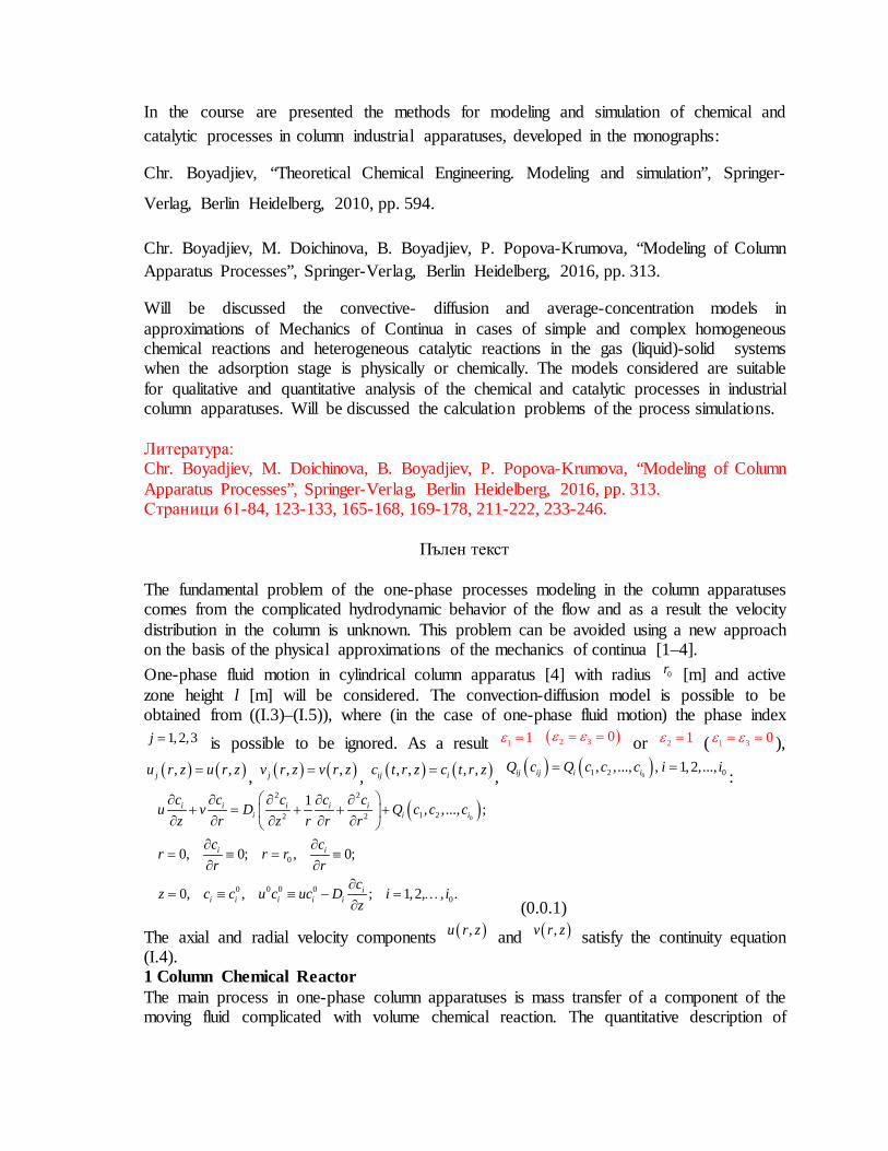
Пълен текст The fundamental problem of the one-phase processes modeling in the column apparatuses comes from the complicated hydrodynamic behavior of the flow and as a result the velocity distribution in the column is unknown. This problem can be avoided using a new approach on the basis of the physical approximations of the mechanics of continua [1–4]. One-phase fluid motion in cylindrical column apparatus [4] with radius 0r [m] and active zone height l [m] will be considered. The convection-diffusion model is possible to be obtained from ((I.3)–(I.5)), where (in the case of one-phase fluid motion) the phase index

1,2,3j = is possible to be ignored. As a result 1 1ε = ( )2 3 0ε ε= = or 2 1ε = ( 1 3 0ε ε= = ), ( ) ( ), ,ju r z u r z= , ( ) ( ), ,jv r z v r z= , ( ) ( ), , , ,ij ic t r z c t r z= , ( ) ( )01 2 0, ,..., , 1, 2,...,ij ij i iQ c Q c c c i i= = :

( )0

2 2

1 22 2

0

0 0 0 00

1 , ,..., ;

0, 0; , 0;

0, , ; 1, 2, , .

i i i i ii i i

i i

ii i i i i

c c c c cu v D Q c c c

z r r rz rc c

r r rr r

cz c c u c uc D i i

z

∂ ∂ ∂ ∂ ∂+ = + + + ∂ ∂ ∂∂ ∂ ∂ ∂

= ≡ = ≡∂ ∂

∂= ≡ ≡ − = …

∂ (0.0.1)

The axial and radial velocity components ( ),u r z and ( ),v r z satisfy the continuity equation (I.4). 1 Column Chemical Reactor The main process in one-phase column apparatuses is mass transfer of a component of the moving fluid complicated with volume chemical reaction. The quantitative description of

this process in column chemical reactors is possible if the axial distribution of the average

concentration ( )c z over the cross-sectional area of the column is known:

( ) ( ) ( )0

00

0

, 0 , 0 , ,

, ,

l

ll

c c z z l c c c l c

c cG c cc

= ≤ ≤ = =

−= >

(0.1.1)

where ( )0z z l= = is the column inlet (outlet) and G is the conversion degree. Two main problems are possible to be solved on this basis: - modeling (design) problem, i.e., to obtain l if G and 0c are given; - simulation (control) problem, i.e., to obtain G if l and 0c are given. The axial distribution of the average concentration ( )c z is to be obtained as a solution of the mass transfer model equations. The modeling problems of the column chemical reactors are possible to be solved using a convection-diffusion type model. 1.1 Convection-diffusion type model In the stationary case the convection-diffusion model of a two component chemical reaction in the column apparatuses [3] has the form:

( )

2 2

1 22 2

1 , , 1, 2,i i i i ii i

c c c c cu v D Q c c i

z r r rz r ∂ ∂ ∂ ∂ ∂

+ = + + + = ∂ ∂ ∂∂ ∂ (0.1.2) where , 1, 2,iD i = are the diffusivities of the reagents in the fluid [m2.s−1]. The axial and radial velocity components ( ),u r z and ( ),v r z satisfy the continuity equation:

( ) ( )0 00; , , 0, 0, ,0 .u v v r r v r z z u u r

z r r∂ ∂

+ + = = ≡ = ≡∂ ∂ (0.1.3)

The model of the mass transfer processes in the column apparatuses (2.1.2) includes boundary conditions, which express a symmetric concentration distribution ( 0r = ), impenetrability of the column wall ( 0r r= ), a constant inlet concentration

0 , 1, 2,ic i = [kg-mol.m-3] and mass balance at the column input ( 0z = ), i.e. the inlet mass flow (

0 0iu c ) is

divided into a convective mass flow (0iuc ) and a diffusion mass flow ( ) :i iD c z− ∂ ∂

0

0 0 0 0

0, 0; , 0;

0, , , 1, 2,

i i

ii i i i i

c cr r r

r rc

z c c u c uc D iz

∂ ∂= ≡ = ≡

∂ ∂∂

= ≡ ≡ − =∂ (0.1.4)

where 0u [m.s−1] is the velocity at the column input. In (2.1.4) it is supposed that a symmetric radial velocity distribution will lead to a symmetric concentration distribution,

too. The term ( )1 2, , 1, 2iQ c c i = in (2.1.2) represents the volume chemical reaction rate (chemical kinetics model). The mass transfer efficiency ( ig ) in the column and conversion degree ( iG ) are possible to be obtained using the inlet and outlet average convective mass flux at the cross-sectional area surface in the column:

( ) ( )

00 0

2 0 00 0

2 , , , , 1, 2.r

ii i i i

i

gg u c ru r l c r l dr G i

r u c= − = =∫

(0.1.5) The average values of the velocity at the column cross-sectional area can be presented as

( ) ( ) ( ) ( )0 0

2 20 00 0

2 2, , , ,r r

u z ru r z dr v z rv r z drr r

= =∫ ∫ (0.1.6)

The velocity distributions assume to be presented by the average functions (2.1.6):

( ) ( ) ( ) ( ) ( ) ( ), , , , , ,u r z u z u r z v r z v z v r z= = (0.1.7) where ( ) ( ), , ,u r z v r z represent the radial non-uniformity of the velocity distributions satisfying the conditions:

( ) ( )

0 0

2 20 00 0

2 2, 1, , 1.r r

ru r z dr rv r z drr r

= =∫ ∫

(0.1.8) A differentiation of ( ),u r z in (2.1.7) with respect to z leads to:

.u d u uu u

z d z z∂ ∂

= +∂ ∂

(0.1.9) Practically, the cross-sectional area surface in the columns is a constant and the average

velocity is a constant too ( )00, ,d u d z u u= = i.e. 0u z∂ ∂ ≡ if 0u z∂ ∂ ≡ ( ) ( )( ), .u u r u u r= = In this case (practically 0u z∂ ∂ ≡ in column apparatuses with big radius values, where the laminar boundary layer thickness at the column wall is negligible with respect to the column radius value) from (2.1.3) follows:

00; , 0dv v r r v

dr r+ = = =

(0.1.10) and the solution is ( ) 0v r ≡ . This leads to a new form of the convection-diffusion type model [4]:

( )2 2

1 22 2

0

0 0 0 0

1 , ;

0, 0; , 0;

0, , ; 1, 2.

i i i ii i

i i

ii i i i i

c c c cu D Q c c

z r rz rc c

r r rr r

cz c c u c uc D i

z

∂ ∂ ∂ ∂= + + + ∂ ∂∂ ∂ ∂ ∂

= ≡ = ≡∂ ∂

∂= ≡ ≡ − =

∂ (0.1.11) The presented convection-diffusion type model (2.1.11) is possible to be used for the qualitative analysis of different chemical processes in the column apparatuses. 1.2 Complex chemical reaction kinetics The complex chemical reaction rate is a function of the reagent concentrations. When the reaction rate is denoted by y and the reagent concentrations by 1,..., mx x the next model equation will be used: ( )1,..., .my f x x= (0.1.12) The function f (like models of all physical processes) is invariant regarding the dimension transformations of the reagent concentration, i.e. this mathematical structure is invariant regarding similarity transformations [3]: , 1,..., ,i i ix k x i m= = (0.1.13) i.e.

( ) ( ) ( )( )

1 1 1 1

1

,..., ,..., . ,..., ,

,..., .m m m m

m

ky f k x k x k k f x x

k k k

ϕ

ϕ

= =

= (0.1.14)

From (2.1.14) it follows that f is a homogenous function, i.e. the relation between the dependent and independent variables in the models is possible to be presented (approximated) by a homogenous function, when the model equations are invariant regarding similarity transformations. A short recording of (2.1.14) is:

[ ] [ ] [ ].i i if x k f xf= (0.1.15) The problem consists in finding a function f that satisfies equation (2.1.15). A differentiation of equation (2.1.15) concerning 1k leads to:

[ ] ( )

1 1

.ii

f xf x

k kf∂ ∂

=∂ ∂ (0.1.16)

On the other hand

[ ] [ ] [ ]1

11 1 1 1

.i i if x f x f xx xk x k x

∂ ∂ ∂∂= =

∂ ∂ ∂ ∂ (0.1.17) From (2.1.16) and (2.1.17) follows

[ ] [ ]1 1

1

,ii

f xx b f x

x∂

=∂ (0.1.18)

where

1

1 1

.ik

bkf

=

∂= ∂ (0.1.19)

The equation (2.1.18) is valid for different values of ik including 1ik = ( )1,..., .i m= As a result , 1,...i ix x i m= = and from (2.1.18) follows

1

1 1

1 ,bf

f x x∂

=∂ (0.1.20)

i.e. 1

1 1 .bf c x= (0.1.21) When the above operations are repeated for 2 ,..., mx x the homogenous function f assumes the form: 1

1 ,..., ,mbbmf cx x= (0.1.22)

i.e. the function f is homogenous if it represents a power functions complex and as a result is invariant with respect to similarity (metric) transformations. The result obtained shows that the chemical reaction rate in (2.1.11) is possible to be presented as

( )1 2 1 2, , 1, 2.m ni

i ic

Q c c k c c it

∂= = =

∂ (0.1.23) 1.3 Two components chemical reaction

Let’s consider a complex chemical reaction in the column and ( ),ic r z 1, 2i = are the concentrations [kg-mol.m-3] of the reagents. In this case the model (2.1.11) has the form:

2 2

1 22 2

0

0 0 0 0

1 ;

0, 0; , 0;

0, , , 1, 2.

m ni i i ii i

i i

ii i i i

c c c cu D k c c

z r rz rc c

r r rr r

cz c c u c uc D i

z

∂ ∂ ∂ ∂= + + − ∂ ∂∂ ∂ ∂ ∂

= ≡ = ≡∂ ∂

∂= ≡ ≡ − =

∂ (0.1.24) The qualitative analysis of the model (2.1.24) will be made using generalized variables [3]:

( ) ( ) ( ) ( ) ( ) ( )

( ) ( ) ( ) ( )

00 0 0

20 0

0

, , , ,

, , , 1, 2 , ,i i i i

r r R z lZ u r u r R u U R u r u r R U R

rc r z c r R lZ c C R Z i

lε

= = = = = =

= = = =

(0.1.25)

where ( )0 00 , , , 1, 2ir l u c i = are the characteristic (inherent) scales (maximal or average values)

of the variables. The introduction of the generalized variables (2.1.25) in (2.1.24) leads to:

2 2

1 22 2

1

1Fo Da ;

0, 0; 1, 0;

0, C 1, 1 Pe ;

m ni i i ii i

i i

ii i

C C C CU C C

Z R RZ RC C

R RR R

CZ U

Z

ε

−

∂ ∂ ∂ ∂= + + − ∂ ∂∂ ∂ ∂ ∂

= ≡ = ≡∂ ∂

∂= ≡ ≡ −

∂ (0.1.26)

( ) ( )

1 0 02

0 00

10 0 0 11 2 0

0 2

Fo , Da Da , Pe ,

Da , ; 1, 2,

iii i i i

i

m nii

D l u lDu r

k l cc c iu c

θ

θ

−

−

= = =

= = =

where Fo, Da and Pe are the Fourier, Damkohler and Peclet numbers, respectively. 1.4 Comparison qualitative analysis As already noted [3, 4] when variable scales in (2.1.25) the maximal or average variable values are used. As a result the unity is the order of magnitude of all functions and their derivatives in (2.1.26), i.e. the effects of the physical and chemical phenomena (the contribution of the terms in (2.1.26)), are determined by the orders of magnitude of the dimensionless parameters in (2.1.26). If all equations in (2.1.26) are divided by the dimensionless parameter, which has the maximal order of magnitude, all terms in the model equations will be classified in three parts:

1. The parameter is unity or its order of magnitude is unity, i.e. this mathematical operator represents a main physical effect;

2. The parameter’s order of magnitude is 110− , i.e. this mathematical operator represents a small physical effect;

3. The parameter’s order of magnitude is 210−≤ , i.e. this mathematical operator represents a very small (negligible) physical effect and has to be neglected, because it is not possible to be measured experimentally.

Here and throughout the book it has to be borne in mind that the process (model) is composed of individual effects (mathematical operators) and if their relative role (influence) in the overall process (model) is less than 210− they have to be ignored, because the inaccuracy of the experimental measurements is above 1%. 1.5 Pseudo-first-order reactions

In the cases of big difference between inlet concentrations of the reagents ( )0 01 2c c0 in

(2.1.24) the problem described by (2.1.26) is possible to be solved in zero approximation

with respect to the very small parameter ( )20 10θ θ −= ≤ and as a result 2 20, 1.Da C= ≡ Very often 1m = and from (2.1.26) follows:

2 21 1

2 2

1

1Fo Da ; Fo Pe ;

0, 0; 1, 0; 0, C 1, 1 Pe ;

C C C CU CZ R RZ R

C C CR R Z UR R Z

ε ε − −

−

∂ ∂ ∂ ∂= + + − = ∂ ∂∂ ∂ ∂ ∂ ∂

= ≡ = ≡ = ≡ ≡ −∂ ∂ ∂ (0.1.27)

where 0

1 1, Da DaC C= = and model (2.1.27) of column apparatuses with pseudo-first-order chemical reaction is obtained. The parameters ε and Fo are related with the column radius

0r and as a result the convection-diffusion type of model (2.1.27) is possible to be used for solving the scale-up problem. 1.6 Similarity conditions From (2.1.27) follows that two mass transfer processes in column apparatuses are similar if the parameters values of Fo, Da, Pe and ε are identical, i.e. these parameters are similarity criteria. In the real cases when the difference between two similar processes is in the parameter values 0 0, , , 1, 2,s s sr l u s = from the similarity conditions follows:

200

0 2 00

Fo , Da , Pe , , 1, 2.ss s s s

s s s s

rDl kl u l sDu r u l

ε

= = = = = (0.1.28)

From (2.1.28) follow three expressions for the characteristic velocity:

0 0 00

00

Pe, , , 1, 2,Fo Da

ss s s

ss

krD Du u u srr

εε ε

= = = = (0.1.29)

i.e. the similarity criteria Fo, Da are incompatible, because from (2.1.29) follows, that (at constant values of Fo, Da and ε ) the increase of the radius 0r (from laboratory model to industrial apparatus) leads to decrease and increase of the velocity 0su simultaneously. The increase of the radius 0r is not possible to be compensated by the changes of velocity 0su (practically the change of 0

sr is not possible to be compensated by the changes of D and k ). These results show that the physical modeling is not possible to be used for a quantitative description of the mass transfer processes in column chemical reactors, i.e. the convection-diffusion model with radius

10r is not physical model of the real process with radius

20r if

1 20 0 .r r≠ The similar situation exists in two-phase processes with chemical reaction.

2 Model Approximations The presentation of the models in generalized variables [3] permits to obtain different approximations of the models, i.e. the approximations of small (~ 10−1) and very small (

210−≤ , negligible) parameters. 2.1 Short columns model

For short columns ( )2 1 10 Fo Per lε − −= = is a small parameter ( )110 ,ε −

− i.e. 1 1Pe 10 Fo− −≤ and

for Fo 1≤ the next small parameter is ( )1 1 1Pe Pe 10 .− − −≤ In these cases the problem (2.1.27) is possible to be solved using the perturbation method (see Chapter 7 and [6]):

( ) ( ) ( ) ( ) ( ) ( ) ( )0 1 22, , , , ... ,C R Z C R Z C R Z C R Zε ε= + + + (0.2.1)

where ( ) ( ) ( )0 1 2, , ,...C C C are solutions of the next problems:

( ) ( ) ( )( )

( ) ( )

( )

0 0 020

2

0 0

0

1Fo Da ;

0, 0; 1, 0;

0, C 1.

C C CU CZ R R R

C CR RR R

Z

∂ ∂ ∂= + − ∂ ∂ ∂

∂ ∂= ≡ = ≡

∂ ∂= ≡ (0.2.2)

( ) ( ) ( )( )

( )

( ) ( )

( )

12 2

2 2

1Fo Da Fo ;

0, 0; 1, 0;

0, C 0; 1,2,... .

s s s ss

s s

s

C C C CU CZ R R R Z

C CR RR R

Z s

− ∂ ∂ ∂ ∂= + − + ∂ ∂ ∂ ∂

∂ ∂= ≡ = ≡

∂ ∂= ≡ = (0.2.3)

A multi-step procedure has to be used for solving (2.2.2) and (2.2.3):

1. Solving (2.2.2) and calculating

( )02

2

CZ

∂∂ ;

2. Solving of (2.2.3) and calculating

( )12

2 , 1, 2,... .sC s

Z

−∂=

∂ 2.2 High-column model For high columns ε is a very small parameter and the problem (2.1.27) is possible to be

solved in zero approximation with respect to ( )20 10ε ε −= ≤ , i.e. 1 2Pe 10 Fo− −≤ and for Fo 1≤

the next very small parameter is 1Pe− ( )1 20 Pe 10 ,− −= ≤ i.e. ( )0 :C C=

2

2

1Fo Da ;

0, 0; 1, 0; 0, C 1.

C C CU CZ R R R

C CR R ZR R

∂ ∂ ∂= + − ∂ ∂ ∂ ∂ ∂

= ≡ = ≡ = ≡∂ ∂ (0.2.4)

2.3 Effect of the chemical reaction rate The effect of the chemical reaction rate is negligible if 20 Da 10−= ≤ and from (2.2.4) follows

1.C ≡ When fast chemical reactions take place ( )2Da 10 ,≥ the terms in (2.2.4) must be divided by Da and the approximation 1 20 Da 10− −= ≤ has to be applied. The result is:

2

2

Fo 10 ; 0, 0; 1, 0,Da

dC d C dC dCC R RR dR dR dRdR

= + − = ≡ = ≡

(0.2.5) i.e. the model (2.2.5) is diffusion type. 2.4 Convection types models

In the cases of big values of the average velocity ( )20 Fo 10 ,−= ≤ from the convection-diffusion type model (2.1.27) is possible to obtain a convection type model when putting Fo 0 :=

( ) Da ; 0, C 1.dCU R C Z

dZ= − = ≡

(0.2.6)

3 Effect of the radial non-uniformity of the velocity distribution The radial non-uniformity of the axial velocity distribution influences the conversion degree, concentration distribution and scale effect. 3.1 Conversion degree As an example will be used the case [4] of parabolic velocity distribution (Poiseuille flow):

( )

2

22 2 .o

ru r ur

= −

(0.3.1) From (2.1.25) and (2.3.1) follows

( ) 22 2 .U R R= − (0.3.2) The solutions of the problem (2.2.4) for Da 1,2= and Fo 0, 0.1, 1.0= permits to obtain ( ),C R Z and ( ) ( ) 0 :C Z c z c=

( ) ( )

1

0

2 , .C Z RC Z R dR= ∫ (0.3.3)

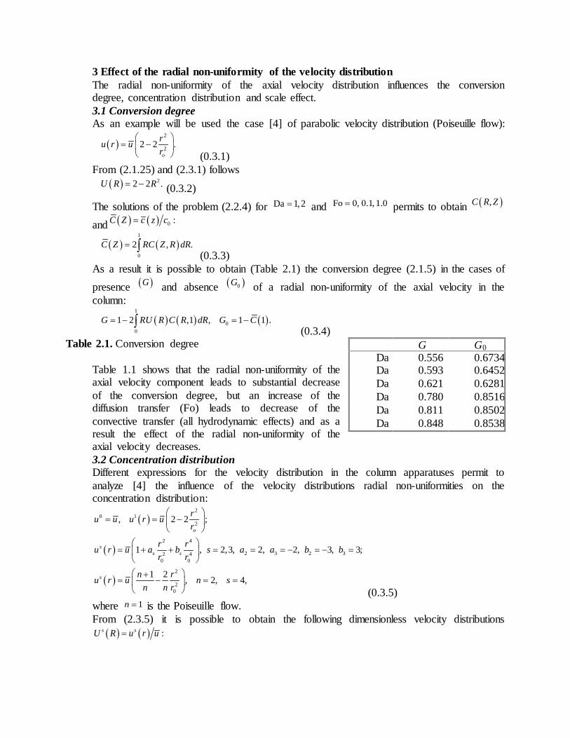
As a result it is possible to obtain (Table 2.1) the conversion degree (2.1.5) in the cases of presence ( )G and absence ( )0G of a radial non-uniformity of the axial velocity in the column:

( ) ( ) ( )

1

00

1 2 ,1 , 1 1 .G RU R C R dR G C= − = −∫ (0.3.4)

Table 2.1. Conversion degree Table 1.1 shows that the radial non-uniformity of the axial velocity component leads to substantial decrease of the conversion degree, but an increase of the diffusion transfer (Fo) leads to decrease of the convective transfer (all hydrodynamic effects) and as a result the effect of the radial non-uniformity of the axial velocity decreases. 3.2 Concentration distribution Different expressions for the velocity distribution in the column apparatuses permit to analyze [4] the influence of the velocity distributions radial non-uniformities on the concentration distribution:

( )

( )

( )

20 1

2

2 4

2 3 2 32 40 0

2

20

, 2 2 ;

1 , 2,3, 2, 2, 3, 3;

1 2 2, ,, 4

o

ss s

s

ru u u r ur

r ru r u a b s a a b br r

n ru r un n r

n s

= = −

= + + = = = − = − =

=

+

= −

= (0.3.5)

where 1n = is the Poiseuille flow. From (2.3.5) it is possible to obtain the following dimensionless velocity distributions

( ) ( ) :s sU R u r u=

G G0 Da

0.556

0.6734 Da

0.593

0.6452 Da

0.621

0.6281 Da

0.780

0.8516 Da

0.811

0.8502 Da

0.848

0.8538

( ) ( ) ( )

( ) ( )

0 1 2 2 2 4

3 2 4 4 2

1, 2 2 , 1 2 3 ,31 2 3 , .2

U R U R R U R R R

U R R R U R R

= = − = + −

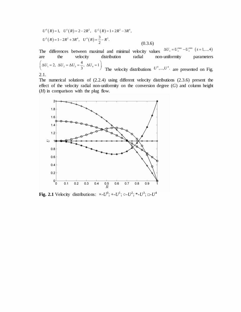
= − + = − (0.3.6)

The differences between maximal and minimal velocity values ( )max minΔ 1,..., 4s s sU U U s= − = are the velocity distribution radial non-uniformity parameters

1 2 3 44Δ 2, Δ Δ , Δ 1 .3

U U U U = = = = The velocity distributions

0 4,..., .U U are presented on Fig. 2.1. The numerical solutions of (2.2.4) using different velocity distributions (2.3.6) present the effect of the velocity radial non-uniformity on the conversion degree (G) and column height (H) in comparison with the plug flow.

Fig. 2.1 Velocity distributions: ×-U0; +-U1; ○-U2; *-U3; □-U4

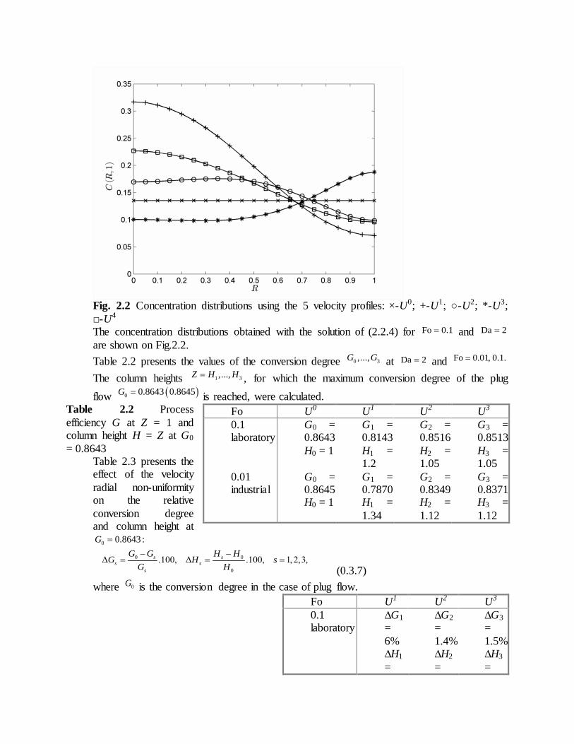
Fig. 2.2 Concentration distributions using the 5 velocity profiles: ×-U0; +-U1; ○-U2; *-U3; □-U4 The concentration distributions obtained with the solution of (2.2.4) for Fo 0.1= and Da 2= are shown on Fig.2.2. Table 2.2 presents the values of the conversion degree 0 3,...,G G at Da 2= and Fo 0.01, 0.1.= The column heights 1 3,...,Z H H= , for which the maximum conversion degree of the plug flow ( )0 0.8643 0.8645G = is reached, were calculated.

Table 2.2 Process efficiency G at Z = 1 and column height H = Z at G0 = 0.8643

Table 2.3 presents the effect of the velocity radial non-uniformity on the relative conversion degree and column height at

0 0.8643 :G =

0 0

0

Δ .100, Δ .100, 1,2,3,s ss s

s

G G H HG H s

G H− −

= = = (0.3.7)

where 0G is the conversion degree in the case of plug flow.

Fo U0 U1

U2 U3 0.1 laboratory

G0 = 0.8643 H0 = 1

G1 = 0.8143 H1 = 1.2

G2 = 0.8516 H2 = 1.05

G3 = 0.8513 H3 = 1.05

0.01 industrial

G0 = 0.8645 H0 = 1

G1 = 0.7870 H1 = 1.34

G2 = 0.8349 H2 = 1.12

G3 = 0.8371 H3 = 1.12

Fo U1 U2 U3

0.1 laboratory

∆G1 = 6% ∆H1 =

∆G2 = 1.4% ∆H2 =

∆G3 = 1.5% ∆H3 =

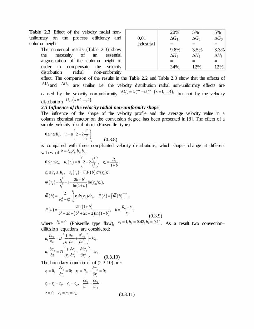
Table 2.3 Effect of the velocity radial non-uniformity on the process efficiency and column height

The numerical results (Table 2.3) show the necessity of an essential augmentation of the column height in order to compensate the velocity distribution radial non-uniformity effect. The comparison of the results in the Table 2.2 and Table 2.3 show that the effects of

2ΔU and 3ΔU are similar, i.e. the velocity distribution radial non-uniformity effects are

caused by the velocity non-uniformity ( )max minΔ 1,..., 4 ,s s sU U U s= − = but not by the velocity distribution ( ), 1,..., 4 .sU s = 3.3 Influence of the velocity radial non-uniformity shape The influence of the shape of the velocity profile and the average velocity value in a column chemical reactor on the conversion degree has been presented in [8]. The effect of a simple velocity distribution (Poiseuille type)

2

0 20

0 , 2 2 rr R u ur

≤ ≤ = −

, (0.3.8) is compared with three complicated velocity distributions, which shapes change at different values of 0 1 2 3, , ,b b b b b= :

( )

( ) ( ) ( )

( ) ( ) ( )

( ) ( ) ( ) ( )

( ) ( )( ) ( )

0

0

201

1 0 1 1 020

0 2 0 2 2 2

2 22

2 2 020

1

2 2 22 20 0

0 02 2

0

0 , 2 2 , ;1

, . . ;

21 ln ,ln 1

2 , ,

2 ln 1, ,

2 2 2 ln 1

R

r

Rrr r u r u rbr

r r R u r u F b r

r b br r rbr

b r r dr F b bR r

b R rF b b

rb b b b b

F

F

F F F−

≤ ≤ = − = + ≤ ≤ =

+= − −

+

= = −

+ −= =

+ − + + +

∫

(0.3.9) where 0 0b = (Poiseuille type flow), 1 2 31, 0.42, 0.11b b b= = = . As a result two convection–diffusion equations are considered:

21 1 1

1 121 1 1

22 2 2

2 222 2 2

1 ,

1 .

c c cu D kcz r r r

c c cu D kcz r r r

∂ ∂ ∂= + − ∂ ∂ ∂

∂ ∂ ∂= + − ∂ ∂ ∂ (0.3.10)

The boundary conditions of (2.3.10) are:

1 21 2 0

1 2

1 21 2 0 1 2

1 2

1 2 0

0, 0; , 0;

, , ;

0, .

c cr r Rr r

c cr r r c cr r

z c c c

∂ ∂= = = =

∂ ∂∂ ∂

= = = =∂ ∂

= = = (0.3.11)

20% 5% 5% 0.01 industrial

∆G1 = 9.8% ∆H1 = 34%

∆G2 = 3.5% ∆H2 = 12%

∆G3 = 3.3% ∆H3 = 12%

The introduction of the dimensionless variables

( ) ( )

1 21 2

0 0

1 1 2 21 1 2 2

1 21 1 2 2

0 0

, , ,

( ) ( )( ) , ( ) ,

, , , ,

r rzZ R RL R R

u r u rU R U Ru uc cC R Z C R Zc c

= = =

= =

= = (0.3.12)

in (2.3.8)-(2.3.11) leads to

( ) ( )

( ) ( ) ( ) ( ) ( )

21 1 1

1 121 1 1

2 21 1 1 1

22 2 2

2 222 2 2

22 2

2 2 2 2

2

1Fo Da ,

12 2 1 , 0 ;1

1Fo Da ,

21 1 ln 1 ,

ln 1

1 1.1

ii

i ii i i

i

i

C C CU CZ R R R

U R b R Rb

C C CU CZ R R R

b bU R F b b R b R

b

Rb

∂ ∂ ∂= + − ∂ ∂ ∂

= − + ≤ ≤+

∂ ∂ ∂= + − ∂ ∂ ∂

+= + − − +

+

≤ ≤+ (0.3.13)

1 21 2

1 2

1 21 2 1 2

1 2

1 2

0, 0; 1, 0;

1 , , , 0,1, 2,3;1

0, 1.i

C CR RR R

C CR R C C ib R R

Z C C

∂ ∂= = = =

∂ ∂∂ ∂

= = = = =+ ∂ ∂

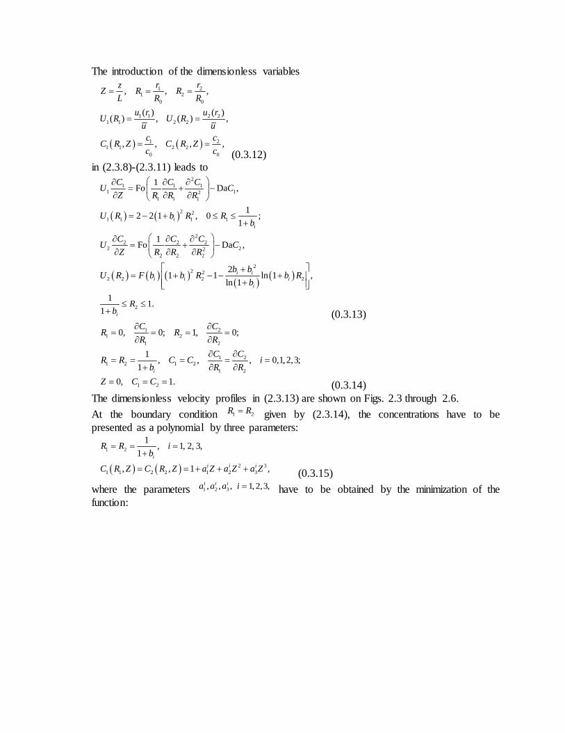
= = = (0.3.14) The dimensionless velocity profiles in (2.3.13) are shown on Figs. 2.3 through 2.6. At the boundary condition 1 2R R= given by (2.3.14), the concentrations have to be presented as a polynomial by three parameters:

( ) ( )

1 2

2 31 1 2 2 1 2 3

1 , 1, 2, 3,1

, , 1 ,i

i i i

R R ib

C R Z C R Z a Z a Z a Z

= = =+

= = + + + (0.3.15) where the parameters 1 2 3, , , 1, 2,3,i i ia a a i = have to be obtained by the minimization of the function:

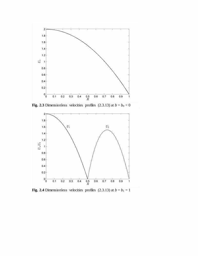
Fig. 2.3 Dimensionless velocities profiles (2.3.13) at b = b0 = 0

Fig. 2.4 Dimensionless velocities profiles (2.3.13) at b = b1 = 1

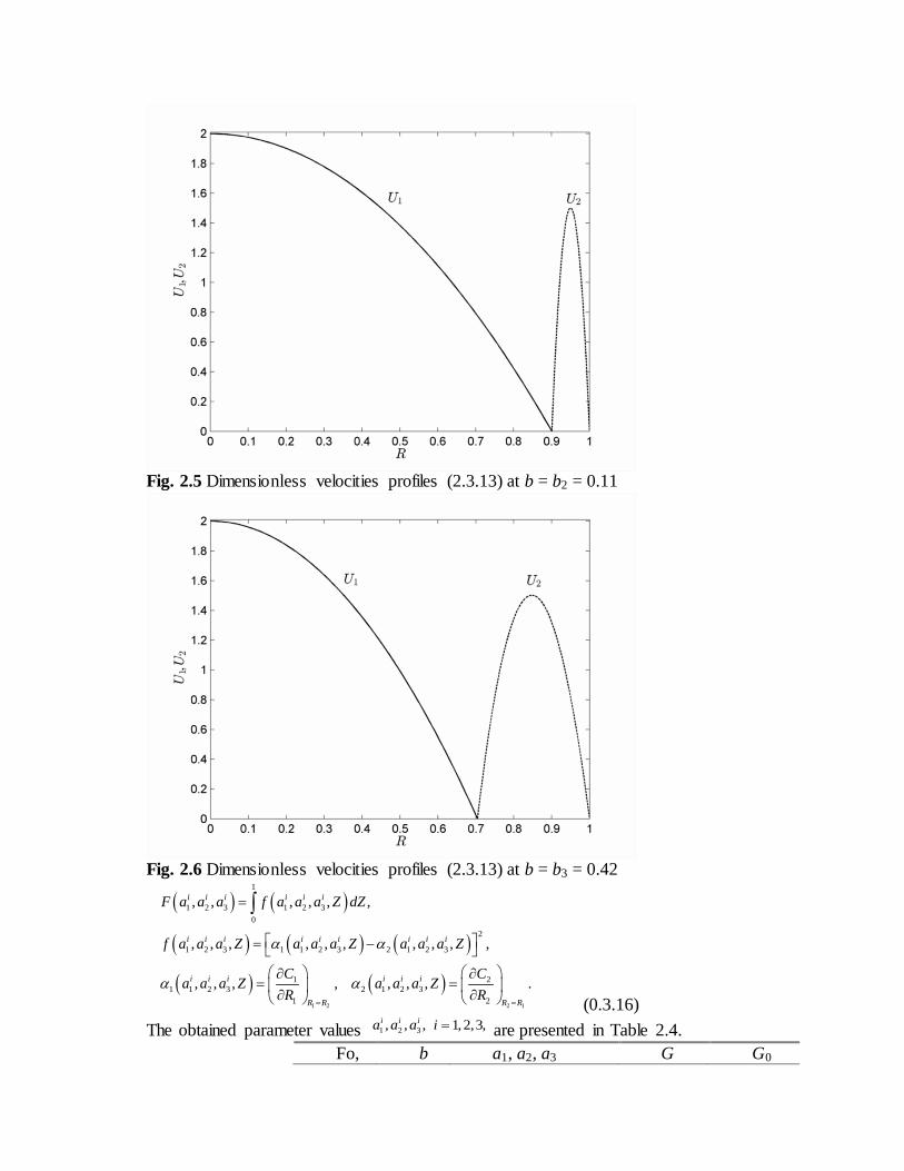
Fig. 2.5 Dimensionless velocities profiles (2.3.13) at b = b2 = 0.11

Fig. 2.6 Dimensionless velocities profiles (2.3.13) at b = b3 = 0.42

( ) ( )

( ) ( ) ( )

( ) ( )1 2 2 1

1

1 2 3 1 2 30

2

1 2 3 1 1 2 3 2 1 2 3

1 21 1 2 3 2 1 2 3

1 2

, , , , , ,

, , , , , , , , , ,

, , , , , , , .

i i i i i i

i i i i i i i i i

i i i i i i

R R R R

F a a a f a a a Z dZ

f a a a Z a a a Z a a a Z

C Ca a a Z a a a ZR R

a a

a a= =

=

= − ∂ ∂

= = ∂ ∂

∫

(0.3.16) The obtained parameter values 1 2 3, , , 1, 2,3,i i ia a a i = are presented in Table 2.4.

Fo, b a1, a2, a3 G G0

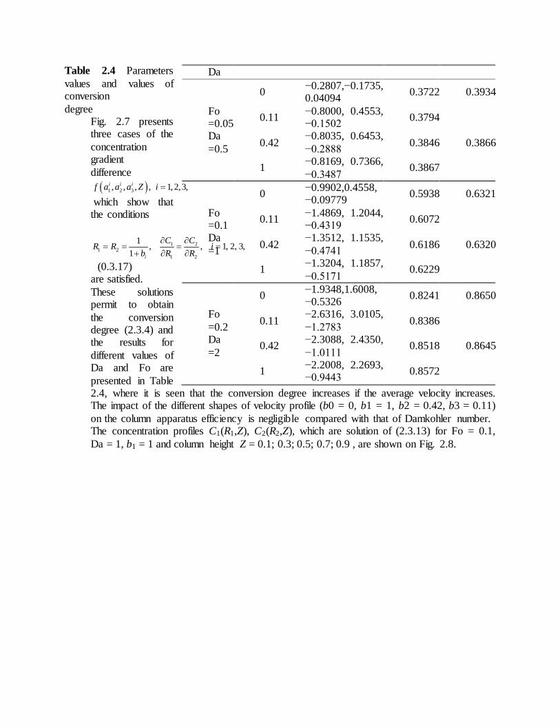
Table 2.4 Parameters values and values of conversion degree

Fig. 2.7 presents three cases of the concentration gradient difference ( )1 2 3, , , , 1, 2,3,i i if a a a Z i =

which show that the conditions

1 21 2

1 2

1 , , 1, 2, 3,1 i

C CR R ib R R

∂ ∂= = = =

+ ∂ ∂

(0.3.17) are satisfied. These solutions permit to obtain the conversion degree (2.3.4) and the results for different values of Da and Fo are presented in Table 2.4, where it is seen that the conversion degree increases if the average velocity increases. The impact of the different shapes of velocity profile (b0 = 0, b1 = 1, b2 = 0.42, b3 = 0.11) on the column apparatus efficiency is negligible compared with that of Damkohler number. The concentration profiles C1(R1,Z), C2(R2,Z), which are solution of (2.3.13) for Fo = 0.1, Da = 1, b1 = 1 and column height Z = 0.1; 0.3; 0.5; 0.7; 0.9 , are shown on Fig. 2.8.

Da 0 −0.2807,−0.1735,

0.04094 0.3722 0.3934

Fo =0.05 0.11 −0.8000, 0.4553,

−0.1502 0.3794

Da =0.5 0.42 −0.8035, 0.6453,

−0.2888 0.3846 0.3866

1 −0.8169, 0.7366, −0.3487 0.3867

0 −0.9902,0.4558, −0.09779 0.5938 0.6321

Fo =0.1 0.11 −1.4869, 1.2044,

−0.4319 0.6072

Da =1 0.42 −1.3512, 1.1535,

−0.4741 0.6186 0.6320

1 −1.3204, 1.1857, −0.5171 0.6229

0 −1.9348,1.6008, −0.5326 0.8241 0.8650

Fo =0.2 0.11 −2.6316, 3.0105,

−1.2783 0.8386

Da =2 0.42 −2.3088, 2.4350,

−1.0111 0.8518 0.8645

1 −2.2008, 2.2693, −0.9443 0.8572

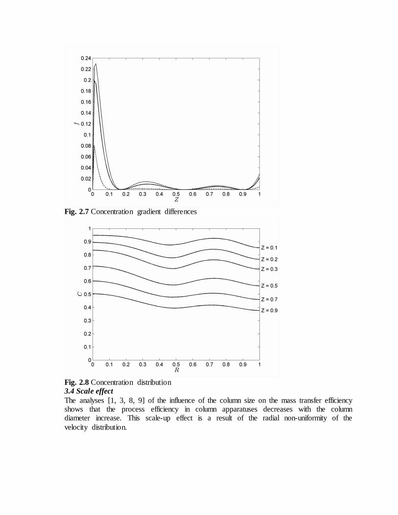
Fig. 2.7 Concentration gradient differences

Fig. 2.8 Concentration distribution 3.4 Scale effect The analyses [1, 3, 8, 9] of the influence of the column size on the mass transfer efficiency shows that the process efficiency in column apparatuses decreases with the column diameter increase. This scale-up effect is a result of the radial non-uniformity of the velocity distribution.

Let us consider “model” column [ ]( )0 0.2 m , Da 2, Fo 0.1r = = = and “industrial” column [ ]( )0 0.5 m , Da 2, Fo 0.01r = = = [7]. The scaling effects on the conversion degrees scaleΔ sG and

column heights scaleΔ :sH mod ind ind mod

scale scalind mod

Δ .100%, Δ .100%, 1,...,3,s s s s

s js s

G G H HG H s

G H− −

= = = (0.3.18)

are possible to be obtained using Table 2.2. The results obtained are shown in Table 1.5. The comparison between the two columns on the basis of (2.3.7) (ΔQmod , ΔQind) and (2.3.18) (ΔHmod , ΔHind) shows that the scale–up leads to decrease of the conversion degree (for constant column height). If consider the columns with constant conversion degree, it leads to the column height increase as result of the column radius increase.

Table 2.5. Comparison of the scaling effect between different velocity profiles

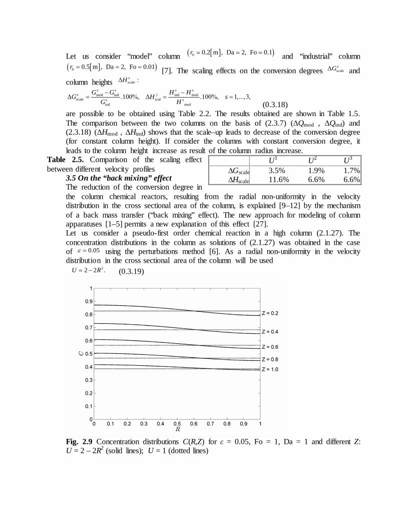
3.5 On the “back mixing” effect The reduction of the conversion degree in the column chemical reactors, resulting from the radial non-uniformity in the velocity distribution in the cross sectional area of the column, is explained [9–12] by the mechanism of a back mass transfer (“back mixing” effect). The new approach for modeling of column apparatuses [1–5] permits a new explanation of this effect [27]. Let us consider a pseudo-first order chemical reaction in a high column (2.1.27). The concentration distributions in the column as solutions of (2.1.27) was obtained in the case of 0.05ε = using the perturbations method [6]. As a radial non-uniformity in the velocity distribution in the cross sectional area of the column will be used 22 2 .U R= − (0.3.19)

Fig. 2.9 Concentration distributions C(R,Z) for ε = 0.05, Fo = 1, Da = 1 and different Z: U = 2 – 2R2 (solid lines); U = 1 (dotted lines)

U1 U2 U3 ∆Gscale 3.5% 1.9% 1.7% ∆Hscale 11.6% 6.6% 6.6%

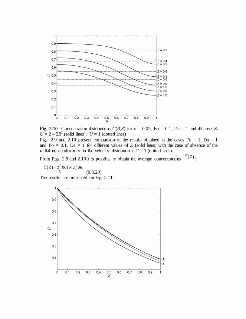
Fig. 2.10 Concentration distributions C(R,Z) for ε = 0.05, Fo = 0.1, Da = 1 and different Z: U = 2 – 2R2 (solid lines); U = 1 (dotted lines) Figs. 2.9 and 2.10 present comparison of the results obtained in the cases Fo = 1, Da = 1 and Fo = 0.1, Da = 1 for different values of Z (solid lines) with the case of absence of the radial non-uniformity in the velocity distribution U = 1 (dotted lines).

From Figs. 2.9 and 2.10 it is possible to obtain the average concentrations ( )C Z :

( ) ( )

1

0

2 , .C Z RC R Z dR= ∫ (0.3.20)

The results are presented on Fig. 2.11.

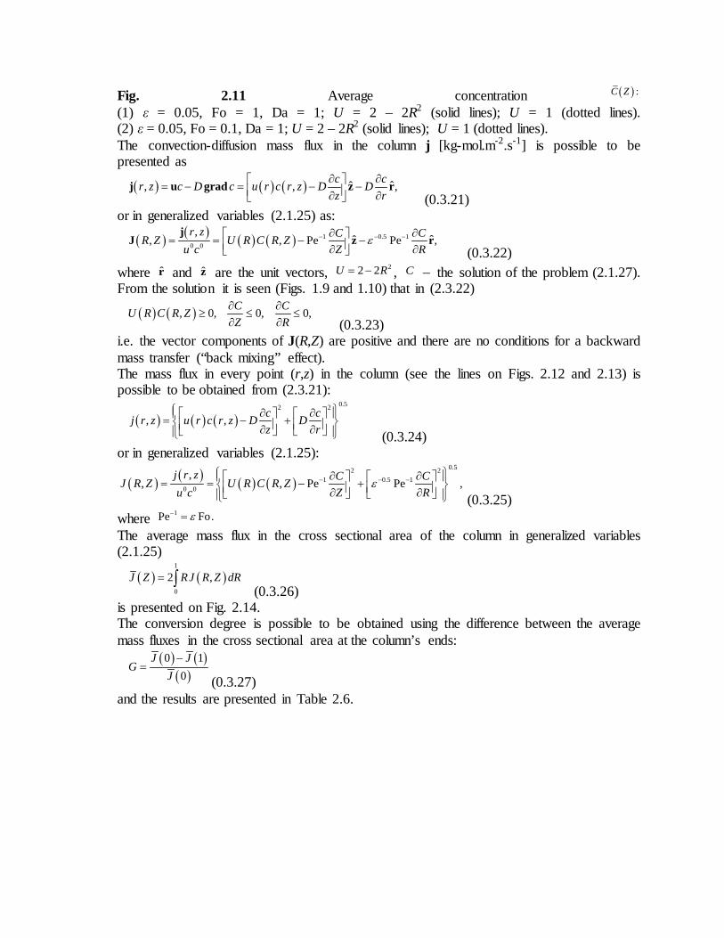
Fig. 2.11 Average concentration ( ) :C Z (1) ε = 0.05, Fo = 1, Da = 1; U = 2 – 2R2 (solid lines); U = 1 (dotted lines). (2) ε = 0.05, Fo = 0.1, Da = 1; U = 2 – 2R2 (solid lines); U = 1 (dotted lines). The convection-diffusion mass flux in the column j [kg-mol.m-2.s-1] is possible to be presented as

( ) ( ) ( ) ˆ ,, ˆ, c cc D c u r c r z D

zr z D

r∂ ∂ − = − − ∂ ∂

=

grad zu rj (0.3.21)

or in generalized variables (2.1.25) as:

( ) ( ) ( ) ( ) 1 0.5 1

0 0

,ˆˆ, , Pe Pe ,

r z C CR Z U R C R ZZ Ru c

ε− − −∂ ∂ = = − − ∂ ∂

jJ z r

(0.3.22) where r and z are the unit vectors, 22 2U R= − , C − the solution of the problem (2.1.27). From the solution it is seen (Figs. 1.9 and 1.10) that in (2.3.22)

( ) ( ), 0, 0, 0,C CU R C R Z

Z R∂ ∂

≥ ≤ ≤∂ ∂ (0.3.23)

i.e. the vector components of J(R,Z) are positive and there are no conditions for a backward mass transfer (“back mixing” effect). The mass flux in every point (r,z) in the column (see the lines on Figs. 2.12 and 2.13) is possible to be obtained from (2.3.21):

( ) ( ) ( )

0 52 .2

, , c cu r c r z D Dz r

j r z ∂ ∂ =

− + ∂ ∂ (0.3.24) or in generalized variables (2.1.25):

( ) ( ) ( ) ( )0.52 2

1 0.5 10 0

,, , Pe Pe ,

j r z C CJ R Z U R C R ZZ Ru c

ε− − − ∂ ∂ = = − + ∂ ∂ (0.3.25)

where 1Pe Fo.ε− = The average mass flux in the cross sectional area of the column in generalized variables (2.1.25)

( ) ( )

1

0

2 ,J Z RJ R Z dR= ∫ (0.3.26)

is presented on Fig. 2.14. The conversion degree is possible to be obtained using the difference between the average mass fluxes in the cross sectional area at the column’s ends:

( ) ( )( )

0 10

J JG

J−

= (0.3.27)

and the results are presented in Table 2.6.

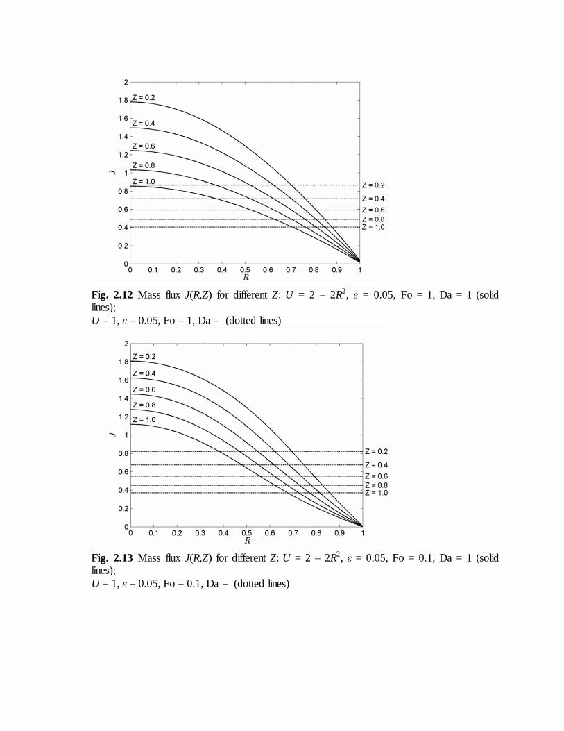
Fig. 2.12 Mass flux J(R,Z) for different Z: U = 2 – 2R2, ε = 0.05, Fo = 1, Da = 1 (solid lines); U = 1, ε = 0.05, Fo = 1, Da = (dotted lines)

Fig. 2.13 Mass flux J(R,Z) for different Z: U = 2 – 2R2, ε = 0.05, Fo = 0.1, Da = 1 (solid lines); U = 1, ε = 0.05, Fo = 0.1, Da = (dotted lines)

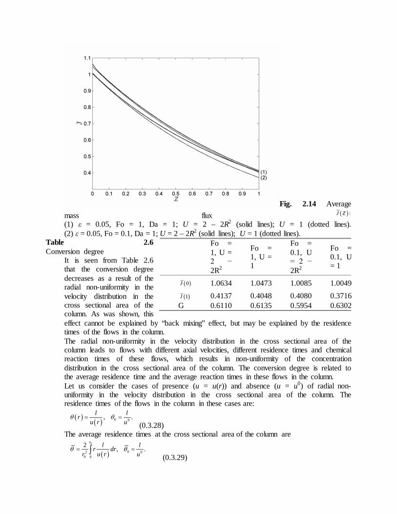
Fig. 2.14 Average mass flux ( ) :J Z (1) ε = 0.05, Fo = 1, Da = 1; U = 2 – 2R2 (solid lines); U = 1 (dotted lines). (2) ε = 0.05, Fo = 0.1, Da = 1; U = 2 – 2R2 (solid lines); U = 1 (dotted lines).

Table 2.6 Conversion degree

It is seen from Table 2.6 that the conversion degree decreases as a result of the radial non-uniformity in the velocity distribution in the cross sectional area of the column. As was shown, this effect cannot be explained by “back mixing” effect, but may be explained by the residence times of the flows in the column. The radial non-uniformity in the velocity distribution in the cross sectional area of the column leads to flows with different axial velocities, different residence times and chemical reaction times of these flows, which results in non-uniformity of the concentration distribution in the cross sectional area of the column. The conversion degree is related to the average residence time and the average reaction times in these flows in the column. Let us consider the cases of presence (u = u(r)) and absence (u = u0) of radial non-uniformity in the velocity distribution in the cross sectional area of the column. The residence times of the flows in the column in these cases are:

( ) ( ) 0 0, .l lr

u r uθ θ= =

(0.3.28) The average residence times at the cross sectional area of the column are

( )0

02 00 0

2 , .r l lr dr

u rr uθ θ= =∫

(0.3.29)

Fo = 1, U = 2 − 2R2

Fo = 1, U = 1

Fo = 0.1, U = 2 − 2R2

Fo = 0.1, U = 1

( )0J 1.0634 1.0473 1.0085 1.0049

( )1J 0.4137 0.4048 0.4080 0.3716 G 0.6110 0.6135 0.5954 0.6302

The using of generalized variables (2.1.25) and 0θ as a scale leads to

( ) ( ) ( )0 0 0 0 0

1, , , 1r RU R

θ θ Θ θ θ Θ Θ Θ= = = = (0.3.30)

and the dimensionless average residence times are:

( )1

00

12 , 1.R dRU R

Θ Θ= =∫ (0.3.31)

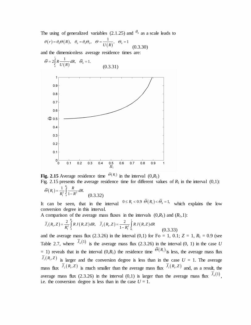
Fig. 2.15 Average residence time ( )1RΘ in the interval (0,R1) Fig. 2.15 presents the average residence time for different values of R1 in the interval (0,1):

( )

1

1 2 21 0

1 .1

R RR dRR R

Θ =−∫

(0.3.32)

It can be seen, that in the interval ( )1 1 00 0.9 1,R RΘ Θ≤ < < = which explains the low conversion degree in this interval. A comparison of the average mass fluxes in the intervals (0,R1) and (R1,1):

( ) ( ) ( ) ( )

1

1

1

1 1 2 12 21 10

2 2, , , , ,1

R

R

J R Z R J R Z dR J R Z R J R Z dRR R

= =−∫ ∫

(0.3.33) and the average mass flux (2.3.26) in the interval (0,1) for Fo = 1, 0.1; Z = 1, R1 = 0.9 (see Table 2.7, where ( )0 1J is the average mass flux (2.3.26) in the interval (0, 1) in the case U = 1) reveals that in the interval (0,R1) the residence time ( )1RΘ is less, the average mass flux

( )1 1,J R Z is larger and the conversion degree is less than in the case U = 1. The average mass flux ( )2 1,J R Z is much smaller than the average mass flux ( )1 1,J R Z and, as a result, the average mass flux (2.3.26) in the interval (0,1) is larger than the average mass flux ( )0 1J , i.e. the conversion degree is less than in the case U = 1.

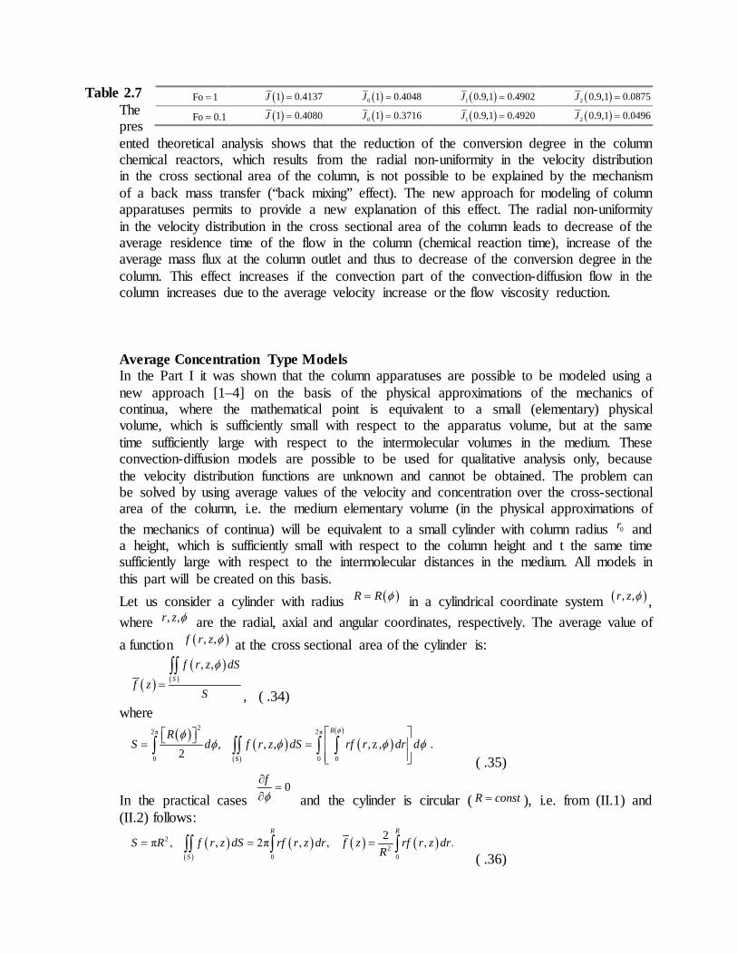
Table 2.7 The presented theoretical analysis shows that the reduction of the conversion degree in the column chemical reactors, which results from the radial non-uniformity in the velocity distribution in the cross sectional area of the column, is not possible to be explained by the mechanism of a back mass transfer (“back mixing” effect). The new approach for modeling of column apparatuses permits to provide a new explanation of this effect. The radial non-uniformity in the velocity distribution in the cross sectional area of the column leads to decrease of the average residence time of the flow in the column (chemical reaction time), increase of the average mass flux at the column outlet and thus to decrease of the conversion degree in the column. This effect increases if the convection part of the convection-diffusion flow in the column increases due to the average velocity increase or the flow viscosity reduction. Average Concentration Type Models In the Part I it was shown that the column apparatuses are possible to be modeled using a new approach [1–4] on the basis of the physical approximations of the mechanics of continua, where the mathematical point is equivalent to a small (elementary) physical volume, which is sufficiently small with respect to the apparatus volume, but at the same time sufficiently large with respect to the intermolecular volumes in the medium. These convection-diffusion models are possible to be used for qualitative analysis only, because the velocity distribution functions are unknown and cannot be obtained. The problem can be solved by using average values of the velocity and concentration over the cross-sectional area of the column, i.e. the medium elementary volume (in the physical approximations of the mechanics of continua) will be equivalent to a small cylinder with column radius 0r and a height, which is sufficiently small with respect to the column height and t the same time sufficiently large with respect to the intermolecular distances in the medium. All models in this part will be created on this basis. Let us consider a cylinder with radius ( )R R f= in a cylindrical coordinate system ( ), ,r z f , where , ,r z f are the radial, axial and angular coordinates, respectively. The average value of a function ( ), ,f r z f at the cross sectional area of the cylinder is:

( )

( )( )

, ,S

f r z dS

f zS

f

=∫∫

, ( .34) where

( )( )

( )( )

( )22π 2π

0 S 0 0

, , , , z , .2

RRS d f r z dS rf r dr d

fff f f f

= =

∫ ∫∫ ∫ ∫ ( .35)

In the practical cases 0f

f∂

=∂ and the cylinder is circular ( R const= ), i.e. from (II.1) and

(II.2) follows:

( )

( )( ) ( ) ( )2

20 0

2π , , 2π , , , .R R

S

S R f r z dS rf r z dr f z rf r z drR

= = =∫∫ ∫ ∫ ( .36)

Fo 1= ( )1 0.4137J = ( )0 1 0.4048J = ( )1 0.9,1 0.4902J = ( )2 0.9,1 0.0875J = Fo 0.1= ( )1 0.4080J = ( )0 1 0.3716J = ( )1 0.9,1 0.4920J = ( )2 0.9,1 0.0496J =

Let us consider a column reactor with radius 0r and height of the active volume l . The average concentration model will be presented on the base of a convection-diffusion model in the case of pseudo-first order chemical reaction. Further, if the fluid circulation takes place, the process is non-stationary and the velocity and concentration distributions in the column must be defined as: ( ) ( ) ( ), , , , , , ,u u r z v v r z c c t r z= = = ( .37) i.e. the convection-diffusion model can be expressed as

( ) ( ) ( ) ( )

2 2

2 2

00

0 0

1 ; 0;

0 0, 0; , 0, 0;

0 ,0 , , , , , .

c c c c c c u v vu v D kct z r r r z r rz r

c ct c c r r r vr r

cz c t,r c t l u u u c t l uc t l Dz

∂ ∂ ∂ ∂ ∂ ∂ ∂ ∂+ + = + + − + + = ∂ ∂ ∂ ∂ ∂ ∂∂ ∂

∂ ∂= ≡ = ≡ = ≡ ≡

∂ ∂∂

= ≡ ≡ ≡ −∂ ( .38)

In (II.5) 0c is the initial concentration, ( ),c t l is the average concentration at the column outlet ( z l= ) and inlet ( 0z = ) (as a result of the fluid circulation in the column), 0u is the average velocity at the column inlet. From (II.3) follow the average values of the velocity and concentration at the column cross-sectional area:

( ) ( ) ( ) ( ) ( ) ( )0 0 0

2 2 20 0 00 0 0

2 2 2, , , , , , , .r r r

u z ru r z dr v z rv r z dr c t z rc t r z drr r r

= = =∫ ∫ ∫ ( .39)

The functions ( ) ( ) ( ), , , , , ,u r z v r z c t r z in (II.5) can be presented with the help of the average functions (II.6):

( ) ( ) ( ) ( ) ( ) ( )( ) ( ) ( )

, , , , , ,

, , , , , ,

u r z u z u r z v r z v z v r z

c t r z c t z c t r z

= =

=

( .40) where ( ) ( ), , ,u r z v r z and ( ), ,c t r z present the radial non-uniformity of the velocity and concentration and satisfy the following conditions:

( ) ( ) ( )

0 0 0

2 2 20 0 00 0 0

2 2 2 , 1, , 1, , , 1.r r r

r u r z dr r v r z dr r c t r z drr r r

= = =∫ ∫ ∫

( .41) The average concentration model may be obtained when putting (II.7) into (II.5), multiplying by r and integrating over r in the interval [ ]00, r . As a result, the following is obtained:

( ) ( ) ( )

( ) ( ) ( )

2

2

0

, , , ;

0, 0, ; 0, ,0 , , 0,

c c ct z u t z u c t z v c D kct z z

ct c z c z c t c t lz

a β γ∂ ∂ ∂+ + + = −

∂ ∂ ∂∂

= ≡ = ≡ ≡∂ ( .42)

where

( ) ( ) ( )

0 0 0

2 2 20 0 00 0 0

2 2 2, , , , , .r r rc ct z rucdr t z ru dr t z rv dr

z rr r ra β γ∂ ∂

= = =∂ ∂∫ ∫ ∫

( .43) The average radial velocity component v can be obtained from the continuity equation in (II.5) if it is multiplied by r2 and then integrated with respect to r over the interval [0, 0r ]:

( )

02

20 0

2, .rd u dv u z r udr

d z d z rdd d= + = ∫

( .44) If (II.11) is put into (II.9), the average concentration model assume the form:

( ) ( ) ( )

2

2

0

;

0, 0, ; 0, ,0 , , 0.

c c d d u cu u c c D kct z d z d z z

ct c z c z c t c t lz

da β γd ∂ ∂ ∂

+ + + + = − ∂ ∂ ∂ ∂

= ≡ = ≡ ≡∂ ( .45)

Practically the cross-sectional area surface in the columns is a constant ( 0r const= ), i.e.

( )0, .d u u u r

d z= =

( .46)

In many practical cases 0u

z∂

=∂

and from (II.7), (II.10) and (II.13) follows:

0, .dv v

d z zd aγ β ∂

= = = = =∂

( .47) As a result from (II.12) is obtained:

( ) ( ) ( )

2

2

0

;

0, 0, ; 0, ,0 , , 0.

c c cu u c D kct z z z

ct c z c z c t c t lz

aa∂ ∂ ∂ ∂+ + = −

∂ ∂ ∂ ∂∂

= ≡ = ≡ ≡∂ ( .48)

In the model (II.15) u is the average velocity of the laminar or turbulent flow in the column, D is the diffusivity or the turbulent diffusivity (as a result of the small scale pulsations). The model parameter a is related with the radial non-uniformity of the velocity distribution and shows the influence of the column radius on the mass transfer kinetics. The parameter k may be obtained beforehand as a result of the chemical kinetics modeling. The parameters in the model (II.15) show the influence of the scale-up (column radius increase) on the mass transfer kinetics if there exists a radial non-uniformity of the velocity distribution. The presented theoretical analysis shows, that in the convection-diffusion and average concentration models, the velocity components and average velocity are: ( ) , 0, .u u r v u const= = = ( .49) The theoretical procedure (II.5–II.15) presented in the Part II will be used for creation of average concentration models of simple and complex chemical processes in one-phase column apparatuses. On this basis the effect of the velocity radial non-uniformity will be analyzed and methods for model parameters identification [1–3] proposed. The convection-diffusion model of the one-phase systems has the form (2.1.11):

( )2 2

1 22 2

0

0 0 0 0

1 , ;

0, 0; , 0;

0, , ; 1, 2.

i i i ii i

i i

ii i i i i

c c c cu D Q c c

z r rz rc c

r r rr r

cz c c u c uc D i

z

∂ ∂ ∂ ∂= + + + ∂ ∂∂ ∂ ∂ ∂

= ≡ = ≡∂ ∂

∂= ≡ ≡ − =

∂ (0.3.50) The average values of the velocity and concentration at the column cross-sectional area in one-phase systems follow from (II.3):

( ) ( ) ( )

0 0

2 20 00 0

2 2 , , 1, 2.r r

i iu ru r dr c z rc r z dr ir r

= = =∫ ∫ (0.3.51)

The functions ( ) ( ), ,iu r c r z can be presented with the help of the average functions (5.0.2): ( ) ( ) ( ) ( ) ( ), , , , 1, 2,i i iu r uu r c r z c z c r z i= = = (0.3.52) where ( )u r and ( ),ic r z represent the radial non-uniformity of the velocity and concentration and satisfy the following conditions:

( ) ( )

0 0

2 20 00 0

2 2 1, , 1, 1, 2.r r

ir u r dr r c r z dr ir r

= = =∫ ∫

(0.3.53) The average concentration model may be obtained if (5.0.3) is put into (5.0.1), multiplied

by r and integrated over r in the interval [ ]00, r . As a result, the average concentration model has the form:

( )02

1 22 20 0

0

0

2 , ;

0, , 0; 1,2.

ri i i

i i i i

ii i

z

d c d d cu u c D rQ c c dr

dz dz dz rdc

z c c idz

aa

=

+ = +

= = = =

∫

(0.3.54) where

( ) ( ) ( )

0

20 0

2 , , 1, 2.r

i iz r u r c r z dr ir

a = =∫

(0.3.55) 1 Simple chemical reactions Let us consider the stationary simple chemical reaction case

2 2

2 2

0

0 0 0 0

1 ;

0, 0; , 0;

0, , .

c c c cu D kcz r rz r

c cr r rr r

cz c c u c uc Dz

∂ ∂ ∂ ∂= + + − ∂ ∂∂ ∂

∂ ∂= ≡ = ≡

∂ ∂∂

= ≡ ≡ −∂ (0.4.1)

1.1 Average concentration model From (II.3) follow the average values of the velocity and concentration at the column cross-sectional area:

( ) ( ) ( )

0 0

2 20 00 0

2 2 , , .r r

u ru r dr c z rc r z drr r

= =∫ ∫ (0.4.2)

The functions ( ) ( ), ,u r c r z in (5.1.1) can be presented with the average functions (5.1.2):

( ) ( ) ( ) ( ) ( ) , , , ,u r u u r c r z c z c r z= = (0.4.3)

where ( )u r and ( ),c r z represent the radial non-uniformity of the velocity and concentration and satisfy the following conditions:

( ) ( )

0 0

2 20 00 0

2 21, , 1.r r

ru r dr rc r z drr r

= =∫ ∫

(0.4.4) The average concentration model may be obtained if (5.1.3) is put into (5.1.1), multiplied

by r and integrated over r in the interval [ ]00, r . As a result, the average concentration model has the form:

( )

2

2

0

;

0, 0 , 0,

d c d d cu u c D kcd z dz dz

d cz c cd z

aa + = −

= = = (0.4.5)

where

( ) ( ) ( )

0

20 0

2 ,r

z ru r c r z drr

a = ∫

(0.4.6) represents effect of the radial non-uniformity of the velocity. The use of the generalized variables

( ) ( ) ( ) ( ) ( )

( ) ( ) ( ) ( ) ( ) ( )( )

( )( )

( ) ( ) ( ) ( ) ( ) ( ) ( )( )

0

0 0

1 1

0 0

, , , ,

, ,, , , , , ,

,2 , Z , 2 ,

u rr r R z lZ u r uU R u r U R

uc r z C R Z

c r z c C R Z c z c C Z c r zc z C Z

C R ZC Z RC R dR z lZ A Z RU R dR

C Za a

= = = = =

= = = =

= = = =∫ ∫

(0.4.7) leads to:

( )2

12Pe Da

0, 1, 0,

dC dA d CA Z C CdZ dZ dZ

dCZ CdZ

−+ = −

= = = (0.4.8)

where Pe and Da are the Peclet and Damkohler numbers, respectively:

, .ul klPe Da

D u= =

(0.4.9) The case of parabolic velocity distribution (Poiseuille flow) will be presented as an example:

( )

20 2

20

2 2 , , 2 2 .ru u u u U R Rr

= − = = −

(0.4.10)

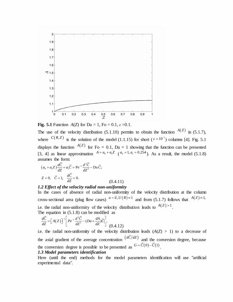
Fig. 5.1 Function A(Z) for Da = 1, Fo = 0.1, ε =0.1. The use of the velocity distribution (5.1.10) permits to obtain the function ( )A Z in (5.1.7), where ( ),C R Z is the solution of the model (1.1.15) for short ( 110ε −= ) columns [4]. Fig. 5.1

displays the function ( )A Z for Fo = 0.1, Da = 1 showing that the function can be presented [3, 4] as linear approximation 0 1A a a Z= + ( 0 11, 0.254a a= = ). As a result, the model (5.1.8) assumes the form:

( )2

10 1 1 2Pe Da ;

0, 1, 0.

dC d Ca a Z a C CdZ dZ

dCZ CdZ

−+ + = −

= = = (0.4.11)

1.2 Effect of the velocity radial non-uniformity In the cases of absence of radial non-uniformity of the velocity distribution at the column cross-sectional area (plug flow cases) ( ), 1u u U R= ≡ and from (5.1.7) follows that ( ) 1,A Z ≡

i.e. the radial non-uniformity of the velocity distribution leads to ( ) 1A Z > . The equation in (5.1.8) can be modified as

( )

21 1

2 ( ) ,dC d C dAA Z Pe Da CdZ dZdZ

− − = − +

(0.4.12) i.e. the radial non-uniformity of the velocity distribution leads (A(Z) > 1) to a decrease of

the axial gradient of the average concentration ( )dC dZ and the conversion degree, because the conversion degree is possible to be presented as ( ) ( )0 1G C C= − . 1.3 Model parameters identification Here (until the end) methods for the model parameters identification will use "artificial experimental data".

The solution of the model (1.1.27) for short ( 110ε −= ) columns [5], in the case 1Fo 0.1, Da 1, Pe Fo 0.05,ε−= = = = permits to ( ),nC Z R be obtained for different

0.1 , 1,2,...,10nZ n n= = and average concentrations:

( ) ( )

1

0

2 , , 1,...,10.n nC Z RC Z R dR n= =∫ (0.4.13)

As a result it is possible to obtain “artificial experimental data” for different values of Z: ( ) ( ) ( )exp 0.95 0.1 , 1,...10, 0.1 , 1,2,...,10,m

n m n nC Z B C Z m Z n n= + = = = (0.4.14) where 0 1, 1,...,10mB m≤ ≤ = are obtained with a generator of random numbers. The obtained artificial experimental data (5.1.14) are used for illustration of the parameters’ ( 0 1,a a ) identification in the average concentrations models (5.1.11) by minimization of the least-squares functions for different values of Z:

( ) ( ) ( )210

0 1 0 1 exp1

, , , , 0.1 , 1,3,5,mn n n n n n n n

mQ a a C Z a a C Z Z n n

=

= − = = ∑ (0.4.15)

where the values of 0 1( , , )n n nC Z a a are obtained as solutions of (5.1.11) for different 0.1 , 1,3,5nZ n n= = . For the solution of (5.1.11) in the cases of short columns

( )1 1Fo 0.1, Da 1, 10 , Pe Fo 0.01ε ε− −= = = = = the perturbation method is to be used (see Chap. 7 and [5])

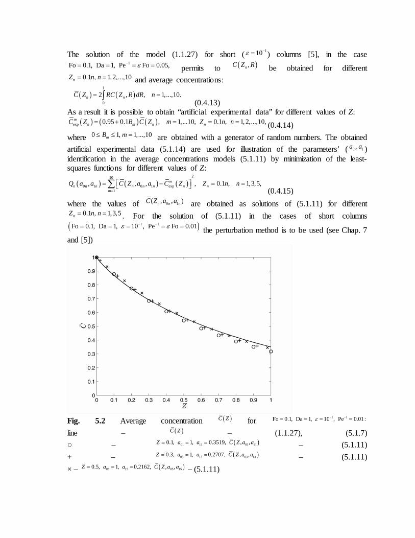
Fig. 5.2 Average concentration ( )C Z for 1 1Fo 0.1, Da 1, 10 , Pe 0.01:ε − −= = = = line – ( )C Z – (1.1.27), (5.1.7) ○ – ( )01 11 01 110.35190.1, 1, , ,,Z a a C Z a a= = = – (5.1.11) + – ( )03 13 03 13 0.27070.3, 1, , ,,Z a a C Z a a= = = – (5.1.11) × – ( )05 15 05 15 0.21620.5, 1, , ,,Z a a C Z a a= = = – (5.1.11)

The solutions 0 1( , )n na a , 1,3,5n = , of the inverse problem for the parameter identification in the two-parameter average concentrations model (5.1.11) for different values of nZ ,

1,3,5n = , after the minimization of (5.1.15), are obtained in [4]. These parameter values are used for the calculations of the average concentration in the model (5.1.11). The obtained values ( )0 1, , ,n n nC Z a a 0.1 , 1,3,5nZ n n= = (the points) are compared (see Fig.5.2) with the

“exact” function (5.1.7) of the average concentration ( )C Z (the line) obtained after solution of the model equation (2.1.27). From Fig.5.2 it is evident that the experimental data, obtained in a short column ( 0.1Z = ) with real diameter, are useful for the model parameters identification. 2 Complex chemical reaction The theoretical procedure (II.5–II.15) is possible to be used for the creation of an average concentration model of the complex chemical processes in one-phase column apparatuses. The base is the convection-diffusion model:

2 2

1 22 2

0

0 0 0 0

1 ;

0, 0; , 0;

0, , , 1, 2.

m ni i i ii

i i

ii i i i

c c c cu D kc c

z r rz rc c

r r rr r

cz c c u c uc D i

z

∂ ∂ ∂ ∂= + + − ∂ ∂∂ ∂ ∂ ∂

= ≡ = ≡∂ ∂

∂= = ≡ − =

∂ (0.5.1) From (II.3) follow the average values of the velocity and concentration functions in (5.2.1) at the column cross-sectional area:

( ) ( ) ( ) ( ) ( )0 0 0

1 1 2 22 2 20 0 00 0 0

2 2 2, , , , .r r r

u ru r dr c z rc r z dr c z rc r z drr r r

= = =∫ ∫ ∫ (0.5.2)

The functions ( ) ( ) ( )1 2, , , ,u r c r z c r z in (4.1.2) can be presented with the help of the average functions (5.2.2):

( ) ( ) ( ) ( ) ( ) ( ) ( ) ( )1 1 1 2 2 2, , , , , ,u r uu r c r z c z c r z c r z c z c r z= = = (0.5.3) where

( ) ( ) ( )

0 0 0

1 22 2 20 0 00 0 0

2 2 21, , 1, , 1.r r r

ru r dr rc r z dr rc r z drr r r

= = =∫ ∫ ∫

(0.5.4) The average concentration model may be obtained when (5.2.3) is put into (5.2.1), multiplied by r and integrated over r in the interval [ ]00, r . As a result, the average concentration model has the form:

( )

2

1 22

0

;

0, 0 , 0, 1, 2,

m ni i ii i i

ii i

d c d d cu u c D kc c

d z dz dzd c

z c c id z

aa d+ = −

= = = = (0.5.5)

where

( ) ( ) ( ) ( ) ( ) ( )0 0

1 22 20 00 0

2 2, , 1, 2; , , .r r

m ni iz ru r c r z dr i z rc r z c r z dr

r ra d= = =∫ ∫

(0.5.6) The using of the generalized variables

( ) ( ) ( ) ( ) ( )

( ) ( ) ( ) ( ) ( ) ( )

( ) ( )( )

( )( )

( ) ( ) ( ) ( ) ( )( )

( ) ( ) ( )( )

( )( )

0

10 0

0

1

0

11 2

1 20

, , , ,

, , , , 2 , Z ,

, ,, ,

,2 , 1, 2,

, ,2 ,

i i i i i i i i

i ii

i i

ii i i

i

m n

u rr r R z lZ u r uU R u r U R

u

c r z c C R Z c z c C Z C Z RC R dR

c r z C R Zc r z

c z C Z

C R Zz lZ A Z RU R dR i

C Z

C R Z C R Zz lZ R dR

C Z C Z

a a

d d

= = = = =

= = =

= =

= = = =

= = ∆ =

∫

∫

∫

(0.5.7) leads to:

( ) ( )2

11 22Pe Da ;

0, 1, 0; 1,2,

m ni i ii i i i

ii

dC dA d CA Z C Z C C

dZ dZ dZdC

Z C idZ

−+ = − ∆

= = = = (0.5.8)

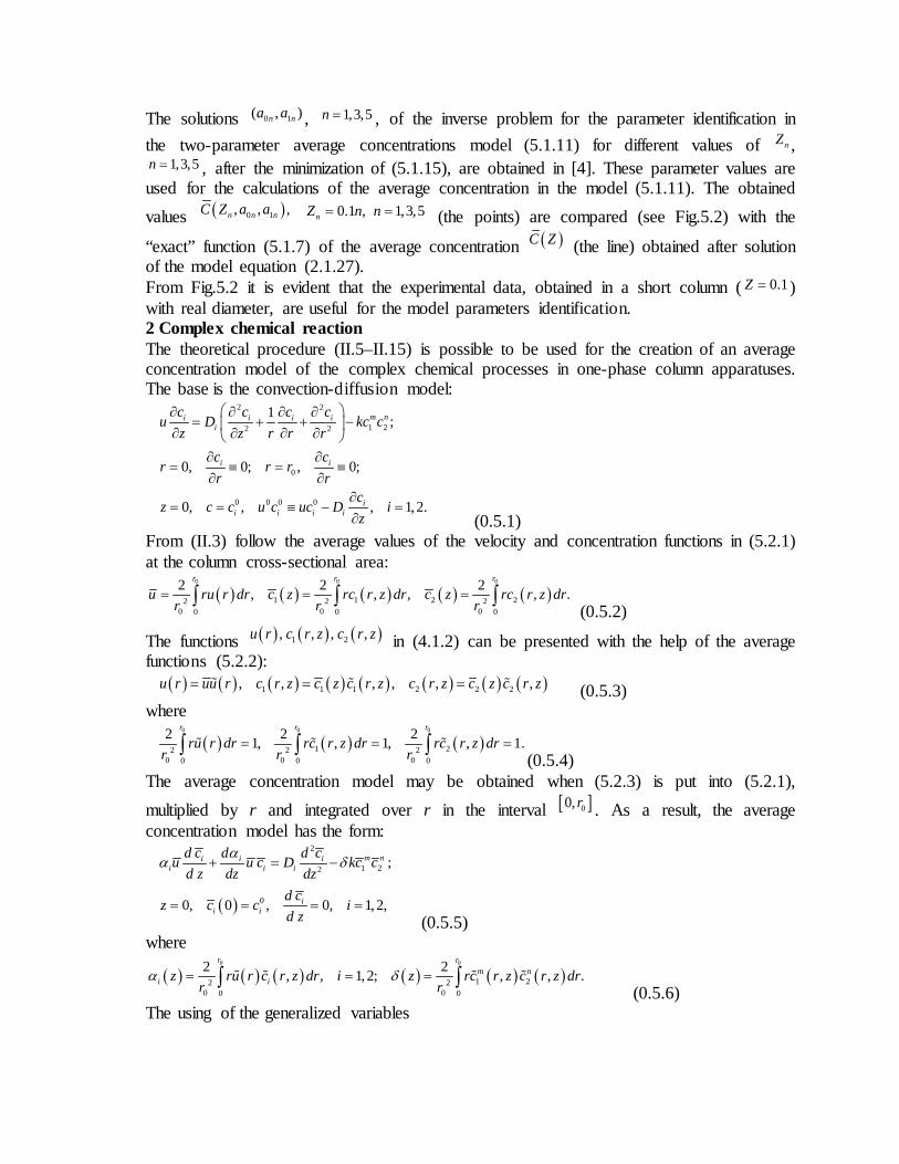
Fig. 5.3 Average concentration ( )1C Z

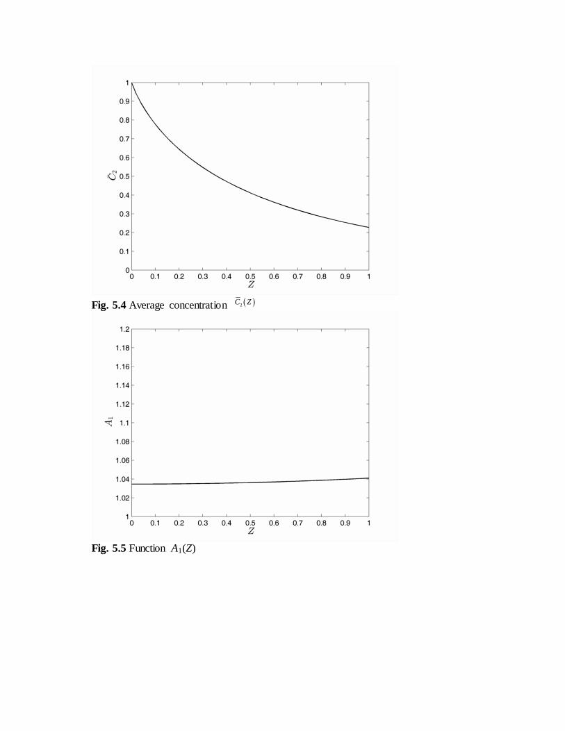
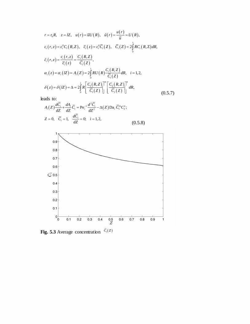
Fig. 5.4 Average concentration ( )2C Z

Fig. 5.5 Function A1(Z)

Fig. 5.6 Function A2(Z)

Fig. 5.7 Function Δ(Z) where Pe and Da are the Peclet and Damkohler numbers, respectively:

( ) ( )

011 0 0 1

1 2 02

Pe , Da Da, Da , ; 1, 2.m ni

i ii

cul kl c c iD u c

θ θ−−= = = = =

(0.5.9) The model (2.1.26) for the high column ( 0ε = ) has the form:

2

1 22

1Fo Da ;

0, 0; 1, 0; 0, C 1.

m ni i ii i

i ii

C C CU C C

Z R R RC C

R R ZR R

∂ ∂ ∂= + − ∂ ∂ ∂ ∂ ∂

= ≡ = ≡ = ≡∂ ∂ (0.5.10)

The solution of (5.2.10) for 1, Fo 0.1, Da 1, 1,2,i im n i= = = = = permits to calculate the

functions ( ) ( ) ( ), , 1, 2,i iC Z A Z i Z= ∆ in (5.2.7). The functions ( ) , 1, 2,iC Z i = are presented on the Figs. 5.3 and 5.4. The functions ( ) ( ), 1, 2,iA Z i Z= ∆ are presented on Figs. 5.5, 5.6 and 5.7, where it is seen that linear approximations are possible to be used: 0 1 0 1, 1, 2,i i iA a a Z i Z= + = ∆ = ∆ + ∆ (0.5.11) and the values of the parameters are:

01 11 02

12 0 1

1.0346, 0.0063, 1.0708,0.1297, 1.0095, 0.0148.

a a aa

= = == ∆ = ∆ = (0.5.12)

3. Catalytic processes The catalytic process is a chemical reaction between three reagents ( 0 3i = ) in gas ( 1j = ), liquid ( 2j = ) or solid ( 3j = ) phase [11]. For definiteness catalytic processes in gas or gas-solid systems will be discussed. The catalytic processes are of heterogeneous or homogeneous type. In the first case the chemical reaction is implemented on a solid catalytic surface, where the first reagent is connected (adsorbed) physically or chemically with the third reagent (catalyst). The adsorption leads to a decrease of the activate energy E of the chemical reaction between the first and second reagents and the chemical reaction rate increases. Analogous effects are possible in the cases of homogeneous chemical reactions, but they are result of the dissolved catalytic substances (third reagent), which change the chemical reaction route and as a result the general activate energy decreases, too. The modeling of the homogeneous catalytic processes is possible to be realized using the model (2.1.12) for three component chemical reaction ( 0 3i = ) and one-phase ( 1j = ) column, where the concentration ( 31c ) of the third reagent (catalyst) is a constant and the catalytic effect is focused in the chemical kinetics term 11 21

m nkc c , where the chemical reaction rate constant k is a function of the catalyst concentration ( 31c ). The heterogeneous catalytic processes are a result of the chemical reaction between two reagents on the catalytic interface, wherein one of them is adsorbed physically or chemically on the free active sites (AS) of the solid catalytic surface. After the chemical reaction the physical (Van der Vaals’s) or chemical (valence) force between the obtained new substance and AS decreases and the new substance (reaction product) is desorbed from the solid surface. As a result the convection-diffusion models of the heterogeneous catalytic processes are possible to be created in the cases of physical adsorption mechanism (2.2.6) and chemical adsorption mechanism (2.2.18). 3.1 Physical adsorption mechanism Let us consider a heterogeneous chemical reaction between two reagents (AC) in gas-solid system, where the first reagent is adsorbed physically on the free active sites (AS) of the solid catalytic surface. The reagents concentrations in the gas phase elementary volume are

11 21,c c [kg-mol.m−3], while in the void elementary volume of the solid phase (catalyst) the concentrations are 13 23,c c . The concentration of the free AS in the solid (catalytic) phase elementary volume is 33c [kg-eq.m−3]. The maximal concentrations of AC and AS are

0 0 011 21 33, ,c c c , where

0 011 21,c c are input AC concentrations in the gas phase. The volume

concentration of the adsorbed AC in the solid phase elementary volume is 033 33c c− .

According the physical adsorption mechanism the gas-solid interphase, the mass transfer rate of the first reagent is ( )01 11 13k c c− , while that of the physical adsorption rate in the solid

phase is 033 33

1 13 2 330 033 33

1c c

bk c k cc c

− −

. The gas-solid interphase mass transfer rate of the second

reagent is ( )02 21 23k c c− , while the catalytic reaction rate is 0

23 33 33( )kc c c− . The difference between the interphase mass transfer coefficients 01 02,k k [s-1] is a result of the difference between the diffusivities of the reagents in the gas phase. The concentration of AS decreases as a result of the physical adsorption and increases as a result of the catalytic reaction, because the reaction product does not have adsorption properties. In the cases of a non-stationary catalytic process the mass balance of AC and AS in the gas and solid phases leads to the convection-diffusion model of a heterogeneous catalytic chemical reaction in a column apparatus:

( )

( )

( )

( )

2 211 11 11 11 11

1 11 01 11 132 2

2 221 21 21 21 21

1 21 02 21 232 2

013 33 3301 11 13 1 13 2 330 0

33 33

2302 21 23

1 ;

1 ;

1 ;

c c c c cu D k c ct z r rz r

c c c c cu D k c ct z r rz r

dc c ck c c bk c k c

dt c cdc

k c c kcdt

∂ ∂ ∂ ∂ ∂+ = + + − − ∂ ∂ ∂∂ ∂

∂ ∂ ∂ ∂ ∂+ = + + − − ∂ ∂ ∂∂ ∂

= − − + −

= − − 023 33 33

0 033 33 331 13 2 33 23 33 330 0

33 33

( );

1 ( ),

c c

dc c cbk c k c kc c c

dt c c

−

= − + − + −

(0.6.1)

where ( )1 1u u r= is the velocity distribution in the gas phase, ( )1 3 1 3, 1ε ε ε ε+ = are the parts of the gas and solid phases in the column volume. The initial and boundary conditions of (2.3.1) are:

( )

( )

0 0 011 11 21 21 13 23 33 33

11 21 11 210

0 0 0 0 1111 11 1 11 1 11 11

0

0 0 0 0 2121 21 1 21 1 21 21

0

0, , , 0, 0, ;

0, 0; , 0;

0, , ,

, ,

z

z

t c c c c c c c cc c c cr r rr r r r

cz c c u c u r c Dz

cc c u c u r c Dz

=

=

= ≡ ≡ ≡ ≡ ≡∂ ∂ ∂ ∂

= = ≡ = = ≡∂ ∂ ∂ ∂

∂ = ≡ ≡ − ∂ ∂ ≡ ≡ − ∂ (0.6.2)

where 01u is the inlet velocity of the gas phase.

For a long duration process the concentration of AS is a constant with respect to the time (as a result of the desorption of the reaction product) and the model (2.3.1) and (2.3.2) is stationary form:

( )

( )

( )

( )

2 211 11 11 11

1 11 01 11 132 2

2 221 21 21 21

1 21 02 21 232 2

033 3301 11 13 0 1 13 2 330 0

33 33

002 21 23 23 33 33

30 1 13

1 ;

1 ;

1 0;

( ) 0;

c c c cu D k c cz r rz r

c c c cu D k c cz r rz r

c ck c c b k c k c

c c

k c c kc c c

cb k c

∂ ∂ ∂ ∂= + + − − ∂ ∂∂ ∂

∂ ∂ ∂ ∂= + + − − ∂ ∂∂ ∂

− − + − =

− − − =

−

( )

( )

0 03 332 33 23 33 330 0

33 33

11 21 11 210

0 0 0 0 1111 11 1 11 1 11 11

0

0 0 0 0 2121 21 1 21 1 21 21

0

1 ( ) 0;

0, 0; , 0;

0, , ,

, .

z

z

ck c kc c c

c cc c c cr r rr r r r

cz c c u c u r c Dz

cc c u c u r c Dz

=

=

+ − + − =

∂ ∂ ∂ ∂

= = ≡ = = ≡∂ ∂ ∂ ∂

∂ = ≡ ≡ − ∂ ∂ ≡ ≡ − ∂ (0.6.3)

The use of dimensionless (generalized) variables [1] permits to make a qualitative analysis of the model (2.3.3), where the inlet velocity and concentrations and the column parameters ( 0 ,r l ) are used as characteristic scales:

1 11110 0

0 1 11

33 13 232121 33 13 230 0 0 0

21 33 11 21

, , , ,

, , , .

u cr zR Z U Cr l u c

c c ccC C C Cc c c c

= = = =

= = = = (0.6.4)

If (2.3.4) is put in (2.3.3) the model in generalized variables takes the form:

( ) ( )

( ) ( )

2 211 11 11 11

11 01 11 132 2

2 221 21 21 21

21 02 21 232 2

1 1

1Fo ;

1Fo ;

0, 0; 1, 0;i i

C C C CU R K C CZ R RZ R

C C C CU R K C CZ R RZ R

C CR R

R R

ε

ε

∂ ∂ ∂ ∂= + + − − ∂ ∂∂ ∂

∂ ∂ ∂ ∂= + + − − ∂ ∂∂ ∂

∂ ∂= ≡ = ≡

∂ ∂ (0.6.5)

( ) 1 1

1 10

0, 1, 1 Pe ; 1,2.ii i

Z

CZ C U R i

Z−

=

∂ = ≡ ≡ − = ∂ ( )

( )11 1 33 5 2321

13 23 332 33 3 33 4 13 5 23

1, , .

1 1 1C K C K CCC C C

K C K C K C K C+ − +

= = =+ + − + + (0.6.6)

In (2.3.5), (2.3.6) the following parameters are used: 20

1 10 0 010 1 1 1 10 0 2 2

01 1 00 0 033 0 1 23 33 0 12 11 2

1 2 3 4 50 0 0 001 01 0211 23 21 33 23 21

, Fo , Pe , 1, 2, Fo Pe ,

, , , , .

i ii i i i i

i

k l D l ru lK iDu u r l

c b k k c b kk c kK K K K Kk k kc k c c k c

ε − −= = = = = =

= = = = = (0.6.7)

For high columns the parameter ε is very small ( 20 10ε −= ≤ ) and the problem (2.3.5) is possible to be solved in zero approximation with respect to ε :

( ) ( )

( ) ( )

211 11 11

11 01 11 132

221 21 21

21 02 21 232

0 00

1Fo ;

1Fo ;

0, 0; 1, 0; 0, 1; 1,2.i ii

C C CU R K C CZ R R R

C C CU R K C CZ R R R

C CR R Z C i

R R

∂ ∂ ∂= + − − ∂ ∂ ∂

∂ ∂ ∂= + − − ∂ ∂ ∂

∂ ∂= ≡ = ≡ = ≡ =

∂ ∂ (0.6.8) For big values of the average velocities

2 211 210 Fo 10 , 0 Fo 10− −= ≤ = ≤ and from (2.3.8) follows

the convective type of model

( ) ( )

( ) ( )

1101 11 13

2102 21 23 0

;

; 0, 1; 1,2.i

dCU R K C CdZ

dCU R K C C Z C idZ

= − −

= − − = ≡ = (0.6.9)

For small values of the average velocities 1 2

00 10 , 1, 2iK i− −= ≤ = , from (2.3.5) follows the diffusion type of model:

( )

( )

2 21 11 11 11

01 11 11 132 2

2 21 21 21 21

02 21 21 232 2

10 Fo ;

10 Fo ;

C C CK C CR RZ R

C C CK C CR RZ R

ε

ε

−

−

∂ ∂ ∂= + + − − ∂∂ ∂

∂ ∂ ∂= + + − − ∂∂ ∂ (0.6.10)

( )

0 0

1 00 0

0

0, 0; 1, 0;

0, 1, 1 Pe ; 1,2.

i i

ii i

Z

C CR R

R RC

Z C U R iZ

−

=

∂ ∂= ≡ = ≡

∂ ∂∂ = ≡ ≡ − = ∂

The solution of the model equations (2.3.6), (2.3.8) requires a velocity distribution in the column. As an example the case of parabolic velocity distribution (Poiseuille flow) in the gas phase will be presented [11]:

( )

22

1 1 20

2 2 , 2 2 .ru u U R Rr

= − = −

(0.6.11) The solution of (2.3.8) depends on the two functions:

( )( )

11 1 33 2113 23

2 33 3 33

1, ,

1 1 1C K C CC C

K C K C+ −

= =+ + − (0.6.12)

where 33C is the solution of the cubic equation:

( ) ( )( )( ) ( )( )( ) ( ) ( )

3 23 33 2 33 1 33 0

3 3 1 4 2 5

2 5 2 2 3 3 4 1 1 3 3 11 2 21

1 4 11 1 3 5 3 2 2 3 2 21

0 21 3 5 5

0,

,

2 2 ,

1 1 2 1 ,.

C C C

K K K K K

K K K K K K K K K K C K C

K C K K K K K K K K CC K K K

ω ω ω ω

ω

ω

ωω

+ + + =

= −

= + − − + + +

= + + + + − − + −

= − − − (0.6.13) As a solution of (2.3.13) 330 1C≤ ≤ is to be used. A solution of the problem (2.3.8), (2.3.12), (2.3.13) has been obtained for the case

0 0 1 2 3 4 51, Fo 0.1, 1,2, 2.5, 1, 1, 0.5, 1i iK i K K K K K= = = = = = = = (0.6.14) as five-matrix forms:

( ) ( ) ( )( ) ( )

11 11( ) 21 21( ) 13 13( )

23 23( ) 33 33( )

0 0 0 00 0

, , , , , ,

, , , ;

1 1, 1,2,..., ; , 1, 2,..., , .1 1

C R Z C C R Z C C R Z C

C R Z C C R Z C

R Z

ρζ ρζ ρζ

ρζ ρζ

ρ ζρ ρ ζ ζ ρ ζρ ζ

= = =

= =

− −= = = = =

− − (0.6.15)

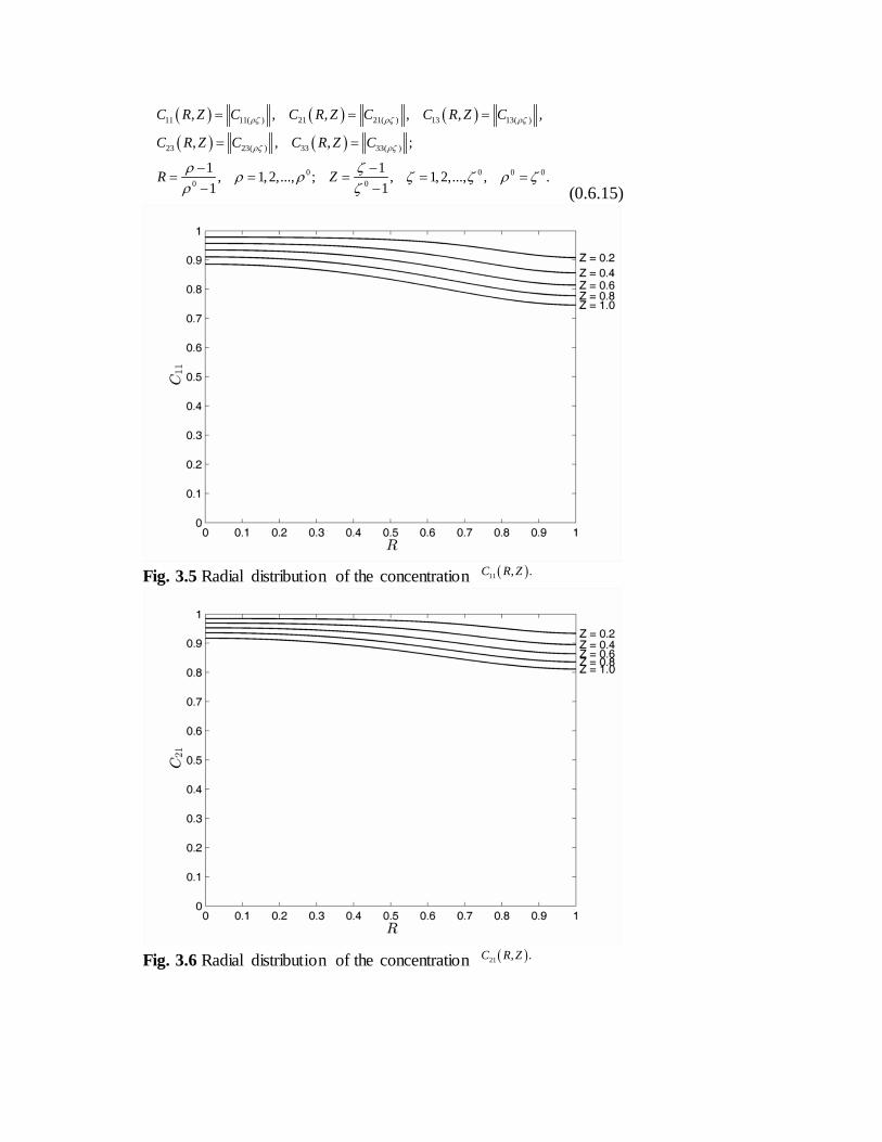
Fig. 3.5 Radial distribution of the concentration ( )11 , .C R Z

Fig. 3.6 Radial distribution of the concentration ( )21 , .C R Z

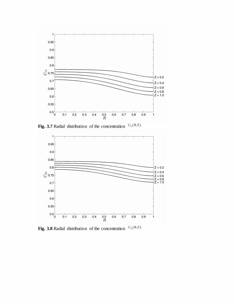
Fig. 3.7 Radial distribution of the concentration ( )13 , .C R Z

Fig. 3.8 Radial distribution of the concentration ( )23 , .C R Z

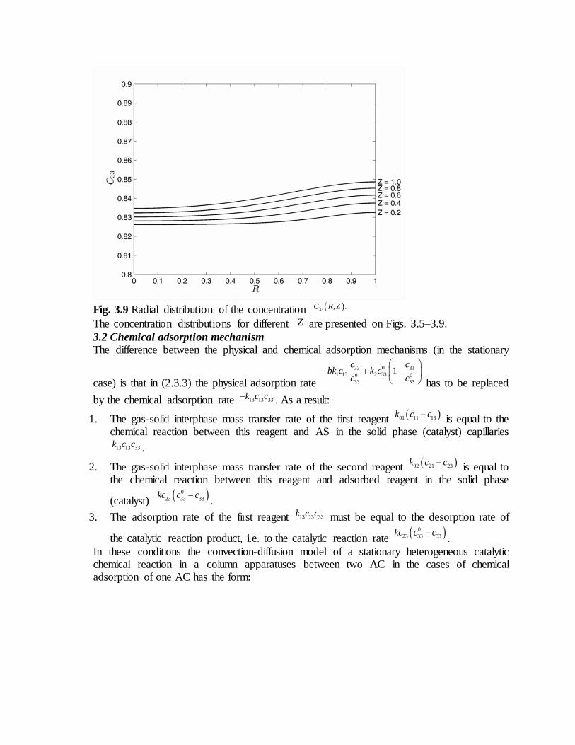
Fig. 3.9 Radial distribution of the concentration ( )33 , .C R Z The concentration distributions for different Z are presented on Figs. 3.5–3.9. 3.2 Chemical adsorption mechanism The difference between the physical and chemical adsorption mechanisms (in the stationary

case) is that in (2.3.3) the physical adsorption rate 033 33

1 13 2 330 033 33

1c c

bk c k cc c

− + −

has to be replaced by the chemical adsorption rate 13 13 33k c c− . As a result:

1. The gas-solid interphase mass transfer rate of the first reagent ( )01 11 13k c c− is equal to the chemical reaction between this reagent and AS in the solid phase (catalyst) capillaries

13 13 33k c c .

2. The gas-solid interphase mass transfer rate of the second reagent ( )02 21 23k c c− is equal to the chemical reaction between this reagent and adsorbed reagent in the solid phase

(catalyst) ( )023 33 33kc c c− .

3. The adsorption rate of the first reagent 13 13 33k c c must be equal to the desorption rate of

the catalytic reaction product, i.e. to the catalytic reaction rate ( )023 33 33kc c c− .

In these conditions the convection-diffusion model of a stationary heterogeneous catalytic chemical reaction in a column apparatuses between two AC in the cases of chemical adsorption of one AC has the form:

( )

( )

( )

2 211 11 11 11

1 11 01 11 132 2

2 221 21 21 21

1 21 02 21 232 2

11 21 11 210

0 0 0 0 1111 11 1 11 1 11 11

0

1 ;

1 ;

0, 0; , 0;

0, ,z

c c c cu D k c cz r rz r

c c c cu D k c cz r rz r

c c c cr r rr r r r

cz c c u c u r c Dz =

∂ ∂ ∂ ∂= + + − − ∂ ∂∂ ∂

∂ ∂ ∂ ∂= + + − − ∂ ∂∂ ∂ ∂ ∂ ∂ ∂

= = ≡ = = ≡∂ ∂ ∂ ∂

∂ = ≡ ≡ − ∂

( )0 0 0 0 2121 21 1 21 1 21 21

0

,

, .z

cc c u c u r c Dz =

∂ ≡ ≡ − ∂ (0.6.16)

( ) ( ) ( )( )

001 11 13 13 13 33 02 21 23 23 33 33

013 13 33 23 33 33

; ;

.

k c c k c c k c c kc c c

k c c kc c c

− = − = −

= − (0.6.17) The introduction of the dimensionless variables (2.3.4) in (2.3.16), (2.3.17) leads to:

( ) ( )

( ) ( )

( )

2 211 11 11 11

11 01 11 132 2

2 221 21 21 21

21 02 21 232 2

1 1

1 11 1

0

1Fo ;

1Fo ;

0, 0; 1, 0;

0, 1, 1 Pe ; 1, 2.

i i

ii i

Z

C C C CU R K C CZ R RZ R

C C C CU R K C CZ R RZ R

C CR R

R RC

Z C U R iZ

ε

ε

−

=

∂ ∂ ∂ ∂= + + − − ∂ ∂∂ ∂

∂ ∂ ∂ ∂= + + − − ∂ ∂∂ ∂

∂ ∂= ≡ = ≡

∂ ∂∂ = ≡ ≡ − = ∂ (0.6.18)

( )2311 21

13 23 331 33 2 33 23 3 13

, , ,1 1 1

CC CC C CK C K C C K C

= = =+ + − + (0.6.19)

where

0 0 013 33 23 33 13 11

1 2 3 001 02 23 21

, , .k c k c k c

K K Kk k k c

= = = (0.6.20)

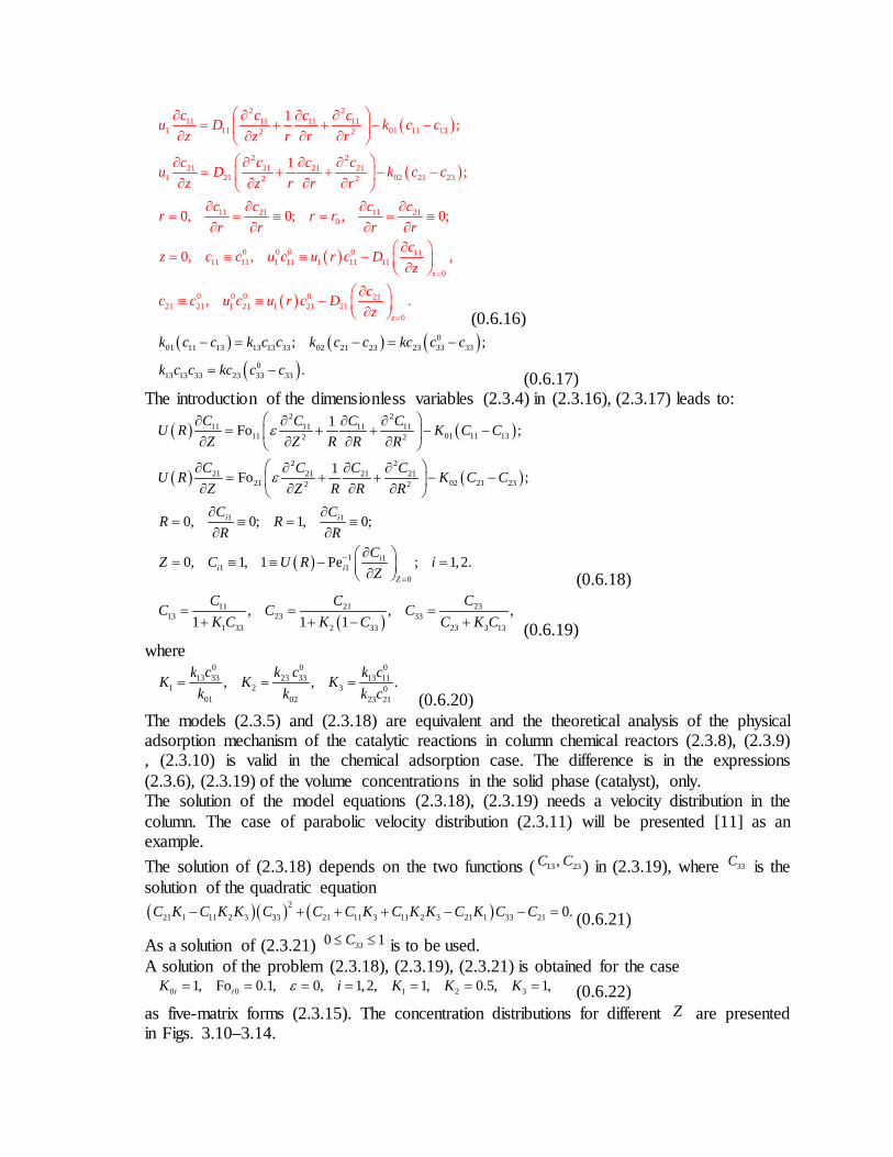
The models (2.3.5) and (2.3.18) are equivalent and the theoretical analysis of the physical adsorption mechanism of the catalytic reactions in column chemical reactors (2.3.8), (2.3.9), (2.3.10) is valid in the chemical adsorption case. The difference is in the expressions (2.3.6), (2.3.19) of the volume concentrations in the solid phase (catalyst), only. The solution of the model equations (2.3.18), (2.3.19) needs a velocity distribution in the column. The case of parabolic velocity distribution (2.3.11) will be presented [11] as an example. The solution of (2.3.18) depends on the two functions ( 13 23,C C ) in (2.3.19), where 33C is the solution of the quadratic equation ( )( ) ( )2

21 1 11 2 3 33 21 11 3 11 2 3 21 1 33 21 0.C K C K K C C C K C K K C K C C− + + + − − = (0.6.21) As a solution of (2.3.21) 330 1C≤ ≤ is to be used. A solution of the problem (2.3.18), (2.3.19), (2.3.21) is obtained for the case 0 0 1 2 31, Fo 0.1, 0, 1,2, 1, 0.5, 1,i iK i K K Kε= = = = = = = (0.6.22) as five-matrix forms (2.3.15). The concentration distributions for different Z are presented in Figs. 3.10–3.14.

The presented new approach for modeling of two-phase processes in column apparatuses is a basis for qualitative analysis of particular processes and for the creation of the average concentration models and quantitative analysis of the processes. Catalytic processes modeling 3.1 Physical adsorption mechanism The convection-diffusion model of the catalytic processes in the column apparatuses [8] in the cases of physical adsorption mechanism has the form (3.3.3):

( )

( )

( )

( )

2 211 11 11 11

1 11 01 11 132 2

2 221 21 21 21

1 21 02 21 232 2

033 3301 11 13 0 1 13 2 330 0

33 33

002 21 23 23 33 33

30 1 13

1 ;

1 ;

1 0;

( ) 0;

c c c cu D k c cz r rz r

c c c cu D k c cz r rz r

c ck c c b k c k c

c c

k c c kc c c

cb k c

∂ ∂ ∂ ∂= + + − − ∂ ∂∂ ∂

∂ ∂ ∂ ∂= + + − − ∂ ∂∂ ∂

− − + − =

− − − =

−

( )

( )

0 03 332 33 23 33 330 0

33 33

11 21 11 210

0 0 0 0 1111 11 1 11 1 11 11

0

0 0 0 0 2121 21 1 21 1 21 21

0

1 ( ) 0;

0, 0; , 0;

0, , ,

, .

z

z

ck c kc c c

c cc c c cr r rr r r r

cz c c u c u r c Dz

cc c u c u r c Dz

=

=

+ − + − =

∂ ∂ ∂ ∂

= = ≡ = = ≡∂ ∂ ∂ ∂

∂ = ≡ ≡ − ∂ ∂ ≡ ≡ − ∂ (0.7.1)

From (II.3) follow the average values of the velocity and the concentration functions in (6.3.1) at the column cross-sectional area:

( ) ( ) ( )

( ) ( ) ( ) ( )

( ) ( ) ( ) ( )

0 0

0 0

0 0

1 1 11 112 20 00 0

21 21 13 132 20 00 0

23 23 33 332 20 00 0

2 2, , ,

2 2, , , ,

2 2, , , .

r r

r r

r r

u ru r dr c z rc r z drr r

c z rc r z dr c z rc r z drr r

c z rc r z dr c z rc r z drr r

= =

= =

= =

∫ ∫

∫ ∫

∫ ∫ (0.7.2)

The functions in (6.3.1) can be presented by the average functions (6.3.2):

( ) ( ) ( ) ( ) ( )( ) ( ) ( ) ( ) ( ) ( )( ) ( ) ( ) ( ) ( ) ( )

1 1 1 11 11 11

21 21 21 13 13 13

23 23 23 33 33 33

, , , ,

, , , , , ,

, , , , , .

u r u u r c r z c z c r z

c r z c z c r z c r z c z c r z

c r z c z c r z c r z c z c r z

= =

= =

= =

(0.7.3) where

( ) ( ) ( )

( ) ( ) ( )

0 0 0

0 0 0

1 11 212 2 20 0 00 0 0

13 23 332 2 20 0 00 0 0

2 2 21, , 1, , 1,

2 2 2, 1, , 1, , 1.

r r r

r r r

ru r dr rc r z dr rc r z drr r r

rc r z dr rc r z dr rc r z drr r r

= = =

= = =

∫ ∫ ∫

∫ ∫ ∫

(0.7.4)

The use of (6.3.2), (6.3.3), (6.3.4) and the averaging procedure (6.0.1)–(6.0.5) leads to the average concentration model of the catalytic processes in the column apparatuses in the cases of physical adsorption mechanism:

( )

( )

( )

( )

211 1 11

1 1 1 11 11 01 11 132

221 2 21

2 1 1 21 21 02 21 232

033 3301 11 13 0 1 13 2 330 0

33 33

002 21 23 23 33 23 33

033 330 1 13 2 330

33

;

;

1 0;

0;

1

d c d d cu u c D k c cdz dz dz

d c d d cu u c D k c cdz dz dz

c ck c c b k c k c

c c

k c c kc c kc c

c cb k c k c

c

aa

aa

β

γ

β

+ = − −

+ = − −

− − + − =

− − + =

− + − 023 33 23 330

33

0 011 2111 11 21 21

0 0

0;

0, , 0, , 0.z z

kc c kc cc

d c d cz c c c cdz dz

γ

= =

+ − =

= = = = = (0.7.5)

where

( ) ( ) ( )

( ) ( ) ( )

( ) ( ) ( )

( ) ( ) ( )

0

0

0

0

1 1 1 1120 0

2 2 1 2120 0

13 3320 0

23 3320 0

2 , ,

2 , ,

2 , , ,

2 , , .

r

r

r

r

z ru r c r z drr

z ru r c r z drr

z rc r z c r z drr

z rc r z c r z drr

a a

a a

β β

γ γ

= =

= =

= =

= =

∫

∫

∫

∫

(0.7.6) The use of the generalized variables

13 23 3311 2111 21 13 23 330 0 0 0 0

11 21 11 21 33

13 23 3311 2111 21 13 23 330 0 0 0 0

11 21 11 21 33

, , , , , ,

, , , , ,

c c cc czZ C C C C Cl c c c c c

c c cc cC C C C Cc c c c c

= = = = = =

= = = = =

(0.7.7) leads to:

( )

( )

2111 1 11

1 11 1 01 11 132

2121 2 21

2 21 2 02 21 232

11 2111 21

0 0

Pe ;

Pe ;

0, 1, 0, 1, 0.Z Z

dC dA d CA C K C CdZ dZ dZdC dA d CA C K C CdZ dZ dZ

dC dCZ C CdZ dZ

−

−

= =

+ = − −

+ = − −

= = = = =

(0.7.8)

( )( )

11 1 33 2113 23

2 33 3 33

5 2333

4 13 5 23

1, ,

1 1 1

.

C K C CC CBK C K GC

K CC

BK C K GC

+ −= =

+ + −

+=

+ + (0.7.9) The parameters in (6.3.8), (6.3.9) and the new functions have the forms:

000 331 2

0 1 10 00 011 110 0

0 1 23 33 0 1 11 22 3 4 50 0 0

01 02 23 21 33 23 21

, , 1, 2; ,

, , , .

ii i

i

k l cu l kK Pe i KD ku c

b k k c b k c kK K K Kk k k c c k c

= = = =

= = = = (0.7.10)

( ) ( ) ( ) ( ) ( )( )

( ) ( ) ( ) ( )( )

( )( )

( ) ( ) ( ) ( )( )

( )( )

( ) ( ) ( ) ( )

11

10

113 33

13 330

123 33

23 330

1 1

11 11 21 210 0

,2 , 1, 2,

, ,2 ,

, ,2 ,

2 , Z , 2 , Z ,

ii i i

i

C R ZA Z lZ z RU R dR i

C Z

C R Z C R ZB Z lZ z R dR

C Z C Z

C R Z C R ZG Z lZ z R dR

C Z C Z

C Z RC R dR C Z RC R dR

a a

β β

γ γ

= = = =

= = =

= = =

= =

∫

∫

∫

∫ ∫ (0.7.11)

( ) ( ) ( ) ( )

( ) ( )

1 1

13 13 23 230 01

33 330

2 , Z , 2 , Z ,

2 , Z .

C Z RC R dR C Z RC R dR

C Z RC R dR

= =

=

∫ ∫

∫

The use of (5.3.11) and ( ) ( ) ( ) ( ) ( )11 21 13 23 33, , , , , , , , ,C R Z C R Z C R Z C R Z C R Z as a solution of the problem (3.3.8, 3.3.12, 3.3.13) for the case (3.3.14) permits to obtain the average

concentrations ( ) ( ) ( ) ( ) ( )11 21 13 23 33, , , ,C Z C Z C Z C Z C Z and the functions ( ) ( ) ( ), 1, 2, ,iA Z i B Z G Z= . They are presented on Figs. 6.17 and 6.18, where it is seen that the

functions ( ) ( ) ( ), 1, 2, ,iA Z i B Z G Z= can be presented as linear approximations: ( ) ( ) ( )0 1 0 1 0 1, 1, 2, , .i i i i i i iA Z a a Z i B Z b b Z G Z g g Z= + = = + = + (0.7.12) The approximations (“theoretical”) parameters values are presented in Table 6.3, where it is seen that 1, 1B G≡ ≡ , practically. Table 6.3 Parameters values For high columns ( 20 10ε −= ≤ ,

1 21 10 . 10 , 1, 1,2i i iPe Fo Fo iε− −= = ≤ ≤ = )

and the problem (5.3.8) takes the form:

( )

( )

11 11 11 01 11 13

21 22 21 02 21 23 11 21

;

; 0, 1, 1.

dC dAA C K C CdZ dZdC dAA C K C C Z C CdZ dZ

+ = − −

+ = − − = ≡ ≡ (0.7.13)

The solution of (5.3.13) depends on the two functions:

( )( )

11 1 33 2113 23

2 33 3 33

1, ,

1 1 1

C K C CC CBK C K GC

+ −= =

+ + − (0.7.14) where 33C is the solution of the cubic equation:

A1 A2 B G a01 = 1.0090

a02 = 1.0063

b0 = 1.0000

g0 = 1.0000

a11 = 0.0257

a12 = 0.0183

b1 = −0.0003

g1 = −0.0002

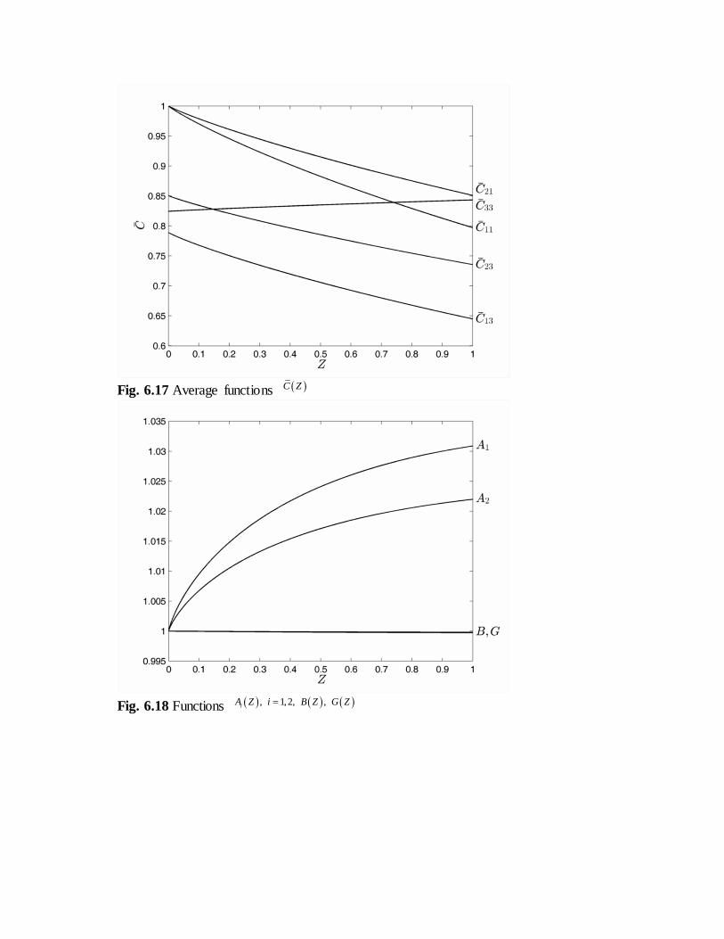
Fig. 6.17 Average functions ( )C Z

Fig. 6.18 Functions ( ) ( ) ( ), 1,2, ,iA Z i B Z G Z=

( ) ( )( )

( )( )

( )( )( ) ( )

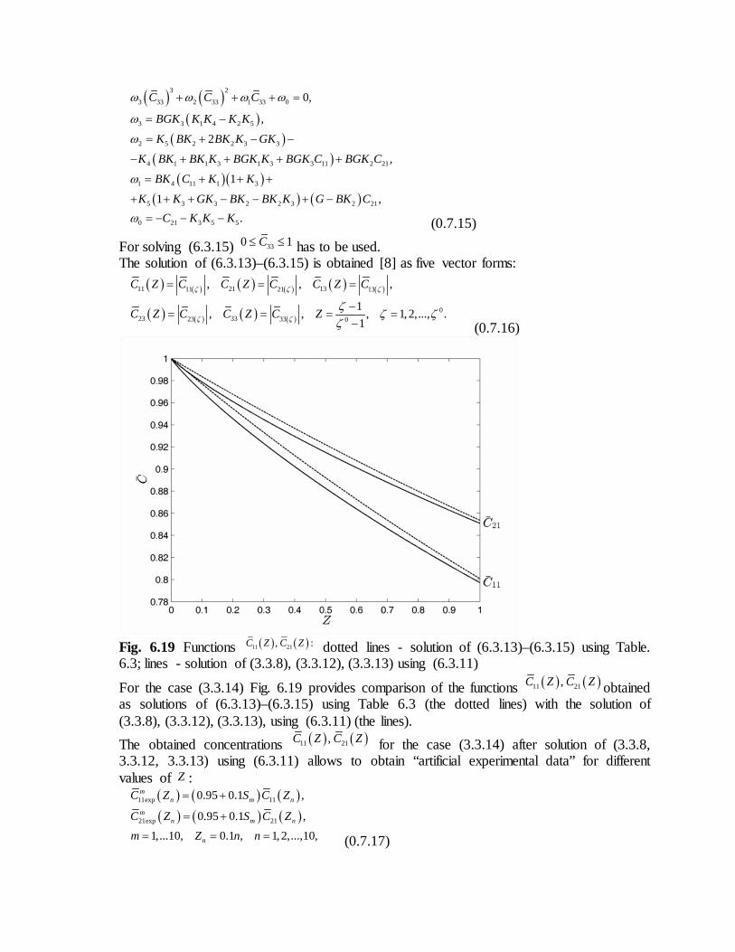
3 2

3 33 2 33 1 33 0

3 3 1 4 2 5

2 5 2 2 3 3

4 1 1 3 1 3 3 11 2 21

1 4 11 1 3

5 3 3 2 2 3 2 21

0 21 3 5 5

0,

,

2

,

1

1 ,.

C C C

BGK K K K K

K BK BK K GK

K BK BK K BGK K BGK C BGK C

BK C K K

K K GK BK BK K G BK CC K K K

ω ω ω ω

ω

ω

ω

ω

+ + + =

= −

= + − −

− + + + +

= + + +

+ + + − − + −

= − − − (0.7.15) For solving (6.3.15) 330 1C≤ ≤ has to be used. The solution of (6.3.13)–(6.3.15) is obtained [8] as five vector forms:

( ) ( ) ( ) ( ) ( ) ( )

( ) ( ) ( ) ( )

11 21 1311 21 13

023 3323 33 0

, , ,

1, , , 1, 2,..., .1

C Z C C Z C C Z C

C Z C C Z C Z

ζ ζ ζ

ζ ζ

ζ ζ ζζ

= = =

−= = = =

− (0.7.16)

Fig. 6.19 Functions ( ) ( )11 21, :C Z C Z dotted lines - solution of (6.3.13)–(6.3.15) using Table. 6.3; lines - solution of (3.3.8), (3.3.12), (3.3.13) using (6.3.11)

For the case (3.3.14) Fig. 6.19 provides comparison of the functions ( ) ( )11 21,C Z C Z obtained as solutions of (6.3.13)–(6.3.15) using Table 6.3 (the dotted lines) with the solution of (3.3.8), (3.3.12), (3.3.13), using (6.3.11) (the lines). The obtained concentrations ( ) ( )11 21,C Z C Z for the case (3.3.14) after solution of (3.3.8, 3.3.12, 3.3.13) using (6.3.11) allows to obtain “artificial experimental data” for different values of Z :

( ) ( ) ( )( ) ( ) ( )

11exp 11

21exp 21

0.95 0.1 ,

0.95 0.1 ,

1,...10, 0.1 , 1,2,...,10,

mn m n

mn m n

n

C Z S C Z

C Z S C Zm Z n n

= +

= +

= = = (0.7.17)

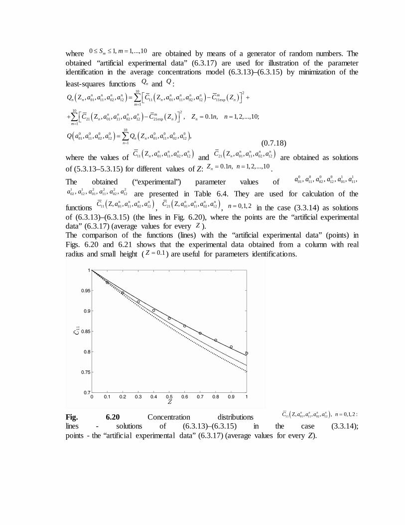
where 0 1, 1,...,10mS m≤ ≤ = are obtained by means of a generator of random numbers. The obtained “artificial experimental data” (6.3.17) are used for illustration of the parameter identification in the average concentrations model (6.3.13)–(6.3.15) by minimization of the least-squares functions nQ and Q :

( ) ( ) ( )

( ) ( )

( ) ( )

10 2

01 11 02 12 11 01 11 02 12 11exp1

10 2

21 01 11 02 12 21exp1

100 0 0 0 0 0 0 001 11 02 12 01 11 02 12

1

Z , , , , Z , , , ,

Z , , , , , 0.1 , 1, 2,...,10;

, , , , , , , ,

n n n n n n n n mn n n n

m

n n n n mn n n

m

n nn

Q a a a a C a a a a C Z

C a a a a C Z Z n n

Q a a a a Q Z a a a a

=

=

=

= − +

+ − = =

=

∑

∑

∑ (0.7.18)

where the values of ( )11 01 11 02 12Z , , , ,n n n nnC a a a a and ( )21 01 11 02 12Z , , , ,n n n n

nC a a a a are obtained as solutions of (5.3.13–5.3.15) for different values of Z: 0.1 , 1, 2,...,10nZ n n= = . The obtained (“experimental”) parameter values of

0 0 0 0 1 101 11 02 12 01 11, , , , , ,a a a a a a

1 1 2 2 2 202 12 01 11 02 12, , , , ,a a a a a a are presented in Table 6.4. They are used for calculation of the

functions ( )11 01 11 02 12Z, , , ,n n n nC a a a a , ( )21 01 11 02 12Z, , , ,n n n nC a a a a , 0,1, 2n = in the case (3.3.14) as solutions of (6.3.13)–(6.3.15) (the lines in Fig. 6.20), where the points are the “artificial experimental data” (6.3.17) (average values for every Z ). The comparison of the functions (lines) with the “artificial experimental data” (points) in Figs. 6.20 and 6.21 shows that the experimental data obtained from a column with real radius and small height ( 0.1Z = ) are useful for parameters identifications.

Fig. 6.20 Concentration distributions ( )11 01 11 02 12Z, , , , , 0,1,2 :n n n nC a a a a n = lines - solutions of (6.3.13)–(6.3.15) in the case (3.3.14); points - the “artificial experimental data” (6.3.17) (average values for every Z).

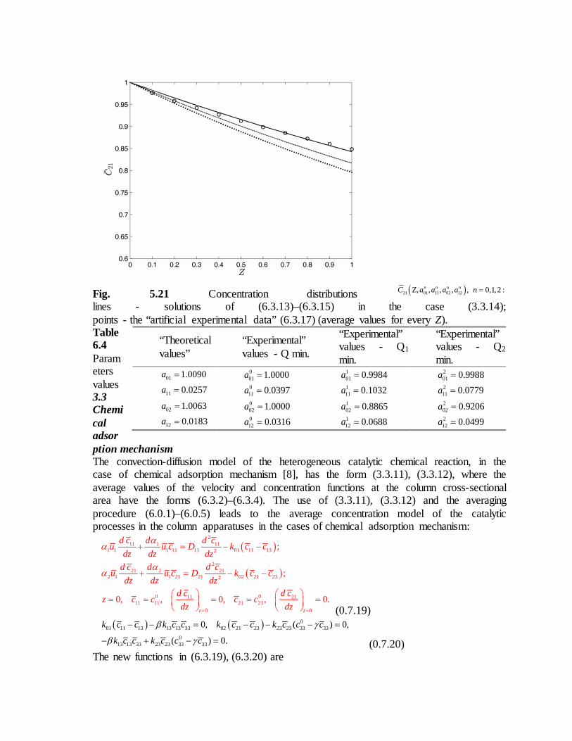
Fig. 5.21 Concentration distributions ( )21 01 11 02 12Z, , , , , 0,1,2 :n n n nC a a a a n = lines - solutions of (6.3.13)–(6.3.15) in the case (3.3.14); points - the “artificial experimental data” (6.3.17) (average values for every Z). Table 6.4 Parameters values 3.3 Chemical adsorption mechanism The convection-diffusion model of the heterogeneous catalytic chemical reaction, in the case of chemical adsorption mechanism [8], has the form (3.3.11), (3.3.12), where the average values of the velocity and concentration functions at the column cross-sectional area have the forms (6.3.2)–(6.3.4). The use of (3.3.11), (3.3.12) and the averaging procedure (6.0.1)–(6.0.5) leads to the average concentration model of the catalytic processes in the column apparatuses in the cases of chemical adsorption mechanism:

( )

( )

211 1 11

1 1 1 11 11 01 11 132

221 2 21

2 1 1 21 21 02 21 232

0 011 2111 11 21 21

0 0

;

;

0, , 0, , 0.z z

d c d d cu u c D k c cdz dz dz

d c d d cu u c D k c cdz dz dz

d c d cz c c c cdz dz

aa

aa

= =

+ = − −

+ = − −

= = = = = (0.7.19)

( ) ( ) 001 11 13 13 13 33 02 21 23 23 23 33 33

013 13 33 23 23 33 33

0, ( ) 0,

( ) 0.

k c c k c c k c c k c c c

k c c k c c c

β γ

β γ

− − = − − − =

− + − = (0.7.20) The new functions in (6.3.19), (6.3.20) are

“Theoretical values”

“Experimental” values - Q min.

“Experimental” values - Q1 min.

“Experimental” values - Q2 min.

01 1.0090a = 001 1.0000a =

101 0.9984a =

201 0.9988a =

11 0.0257a = 011 0.0397a =

111 0.1032a =

211 0.0779a =

02 1.0063a = 002 1.0000a =

102 0.8865a =

202 0.9206a =

12 0.0183a = 012 0.0316a =

112 0.0688a =

212 0.0499a =

( ) ( ) ( )

( ) ( ) ( )

( ) ( ) ( )

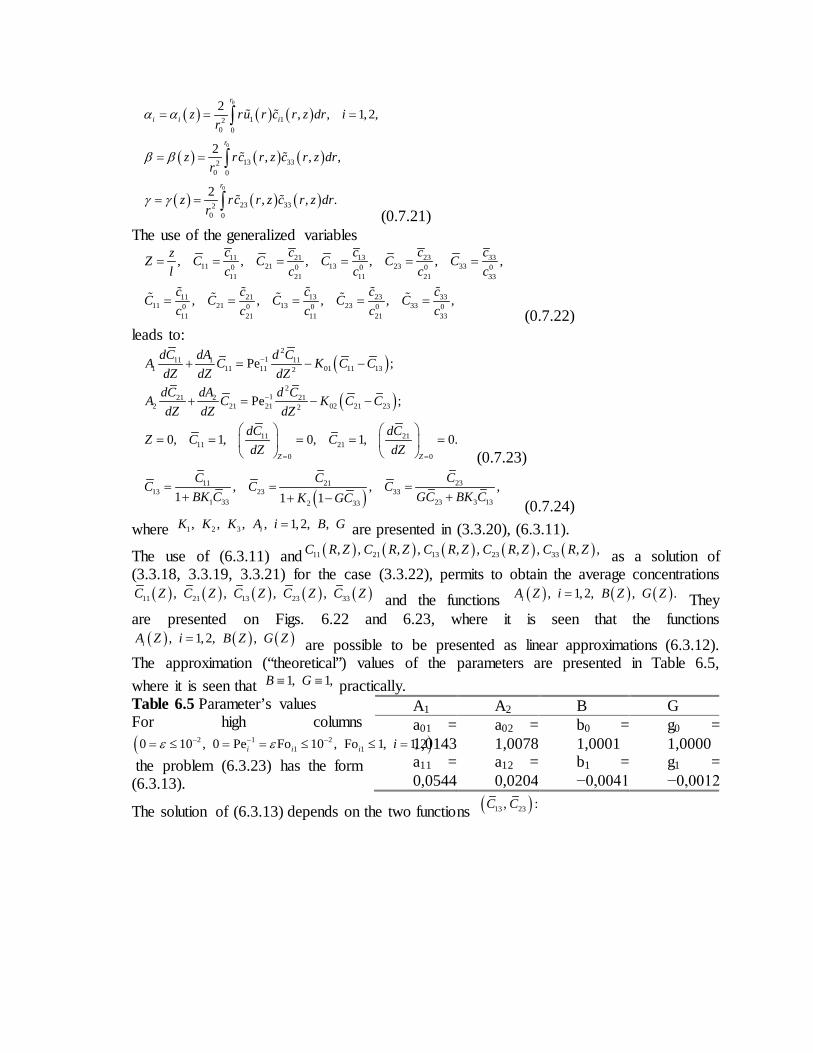
0

0

0

1 120 0

13 3320 0

23 3320 0

2 , , 1, 2,

2 , , ,

2 , , .

r

i i i

r

r

z ru r c r z dr ir

z rc r z c r z drr

z rc r z c r z drr

a a

β β

γ γ

= = =

= =

= =

∫

∫

∫

(0.7.21) The use of the generalized variables

13 23 3311 2111 21 13 23 330 0 0 0 0

11 21 11 21 33

13 23 3311 2111 21 13 23 330 0 0 0 0

11 21 11 21 33

, , , , , ,

, , , , ,

c c cc czZ C C C C Cl c c c c c

c c cc cC C C C Cc c c c c

= = = = = =

= = = = =

(0.7.22) leads to:

( )

( )

2111 1 11

1 11 11 01 11 132

2121 2 21

2 21 21 02 21 232

11 2111 21

0 0

Pe ;

Pe ;

0, 1, 0, 1, 0.Z Z

dC dA d CA C K C CdZ dZ dZdC dA d CA C K C CdZ dZ dZ

dC dCZ C CdZ dZ

−

−

= =

+ = − −

+ = − −

= = = = =

(0.7.23)

( )2311 21

13 23 331 33 23 3 132 33

, , ,1 1 1

CC CC C CBK C GC BK CK GC

= = =+ ++ − (0.7.24)

where 1 2 3, , , , 1, 2, ,iK K K A i B G= are presented in (3.3.20), (6.3.11).

The use of (6.3.11) and ( ) ( ) ( ) ( ) ( )11 21 13 23 33, , , , , , , , , ,C R Z C R Z C R Z C R Z C R Z as a solution of (3.3.18, 3.3.19, 3.3.21) for the case (3.3.22), permits to obtain the average concentrations

( ) ( ) ( ) ( ) ( )11 21 13 23 33, , , ,C Z C Z C Z C Z C Z and the functions ( ) ( ) ( ), 1, 2, , .iA Z i B Z G Z= They are presented on Figs. 6.22 and 6.23, where it is seen that the functions

( ) ( ) ( ), 1, 2, ,iA Z i B Z G Z= are possible to be presented as linear approximations (6.3.12). The approximation (“theoretical”) values of the parameters are presented in Table 6.5, where it is seen that 1, 1,B G≡ ≡ practically. Table 6.5 Parameter’s values For high columns ( )2 1 2

1 10 10 , 0 Pe Fo 10 , Fo 1, 1,2i i i iε ε− − −= ≤ = = ≤ ≤ =

the problem (6.3.23) has the form (6.3.13).

The solution of (6.3.13) depends on the two functions ( )13 23, :C C

A1 A2 B G a01 = 1,0143

a02 = 1,0078

b0 = 1,0001

g0 = 1,0000

a11 = 0,0544

a12 = 0,0204

b1 = −0,0041

g1 = −0,0012

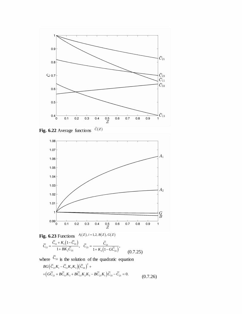
Fig. 6.22 Average functions ( )C Z

Fig. 6.23 Functions ( ) ( ) ( ), 1,2, ,iA Z i B Z G Z=

( )( )

11 1 33 2113 23

2 33 3 33

1, ,

1 1 1

C K C CC CBK C K GC

+ −= =

+ + − (0.7.25) where 33C is the solution of the quadratic equation

( )( )( )

2

21 1 11 2 3 33

21 11 3 11 2 3 21 1 33 21 0.

BG C K C K K C

GC BC K BC K K BC K C C

− +

+ + + − − = (0.7.26)

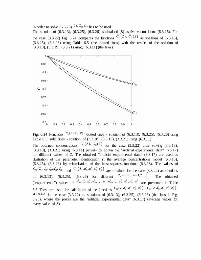
In order to solve (6.3.26) 330 1C≤ ≤ has to be used. The solution of (6.3.13), (6.3.25), (6.3.26) is obtained [8] as five vector forms (6.3.16). For the case (3.3.22) Fig. 6.24 compares the functions ( ) ( )11 21,C Z C Z as solutions of (6.3.13), (6.3.25), (6.3.26) using Table 6.5 (the dotted lines) with the results of the solution of (3.3.18), (3.3.19), (3.3.21) using (6.3.11) (the lines).

Fig. 6.24 Functions ( ) ( )11 21, :C Z C Z dotted lines - solution of (6.3.13), (6.3.25), (6.3.26) using Table 6.5; solid lines - solution of (3.3.18), (3.3.19), (3.3.21) using (6.3.11). The obtained concentrations ( ) ( )11 21,C Z C Z for the case (3.3.22) after solving (3.3.18), (3.3.19), (3.3.21) using (6.3.11) permits to obtain the “artificial experimental data” (6.3.17) for different values of Z. The obtained “artificial experimental data” (6.3.17) are used as illustration of the parameter identification in the average concentrations model (6.3.13), (6.3.25), (6.3.26) by minimization of the least-squares functions (6.3.18). The values of

( )11 01 11 02 12Z , , , ,n n n nnC a a a a and ( )21 01 11 02 12Z , , , ,n n n n

nC a a a a are obtained for the case (3.3.22) as solutions of (6.3.13), (6.3.25), (6.3.26) for different 0.1 , 1,2,...,10.nZ n n= = The obtained (“experimental”) values of

0 0 0 0 1 1 1 1 2 2 2 201 11 02 12 01 11 02 12 01 11 02 12, , , , , , , , , , ,a a a a a a a a a a a a are presented in Table

6.6 They are used for calculation of the functions ( )11 01 11 02 12Z, , , , ,n n n nC a a a a ( )21 01 11 02 12Z, , , , ,n n n nC a a a a 0,1, 2n = in the case (3.3.22) as solutions of (6.3.13), (6.3.25), (6.3.26) (the lines in Fig.

6.25), where the points are the “artificial experimental data” (6.3.17) (average values for every value of Z).

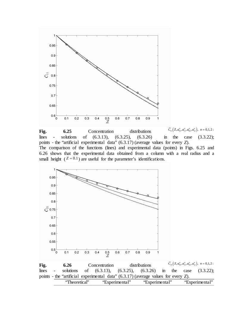
Fig. 6.25 Concentration distributions ( )11 01 11 02 12Z, , , , , 0,1,2 :n n n nC a a a a n = lines - solutions of (6.3.13), (6.3.25), (6.3.26) in the case (3.3.22); points - the “artificial experimental data” (6.3.17) (average values for every Z). The comparison of the functions (lines) and experimental data (points) in Figs. 6.25 and 6.26 shows that the experimental data obtained from a column with a real radius and a small height ( 0.1Z = ) are useful for the parameter’s identifications.

Fig. 6.26 Concentration distributions ( )21 01 11 02 12Z, , , , , 0,1,2 :n n n nC a a a a n = lines - solutions of (6.3.13), (6.3.25), (6.3.26) in the case (3.3.22); points - the “artificial experimental data” (6.3.17) (average values for every Z).

“Theoretical” “Experimental” “Experimental” “Experimental”

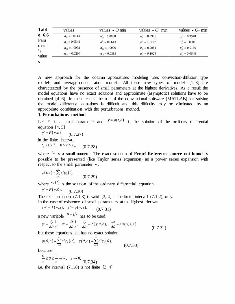
Table 6.6 Parameter’s values A new approach for the column apparatuses modeling uses convection-diffusion type models and average-concentration models. All these new types of models [1–3] are characterized by the presence of small parameters at the highest derivatives. As a result the model equations have no exact solutions and approximate (asymptotic) solutions have to be obtained [4–6]. In these cases the use of the conventional software (MATLAB) for solving the model differential equations is difficult and this difficulty may be eliminated by an appropriate combination with the perturbations method. 1. Perturbations method Let ε is a small parameter and ( ),y tϕ ε= is the solution of the ordinary differential equation [4, 5] ( )' ,y F y ε= (0.7.27) in the finite interval 0 0, 0 ,t t T ε ε≤ ≤ ≤ ≤ (0.7.28) where 0ε is a small numeral. The exact solution of Error! Reference source not found. is possible to be presented (like Taylor series expansion) as a power series expansion with respect to the small parameter ε :

( ) ( )

0, ,s

ss

t tϕ ε ε ϕ∞

=

= ∑ (0.7.29)

where ( )0 tϕ is the solution of the ordinary differential equation ( )' , 0 .y F y= (0.7.30) The exact solution (7.1.3) is valid [3, 4] in the finite interval (7.1.2), only. In the case of existence of small parameters at the highest derivate ( ) ( )' , , ' , ,y f y z z g y zε = = (0.7.31) a new variable tθ ε= has to be used:

( ) ( )1 1' , ' , , , , , , ,dy dz dy dzy z f y z g y z

d d d dε ε ε

θ ε θ ε θ θ= = = =

(0.7.32) but these equations set has no exact solution

( ) ( ) ( ) ( )

0 0, , , ,s s

s ss s

ϕ θ ε ε ϕ θ γ θ ε ε γ θ∞ ∞

= =

= =∑ ∑ (0.7.33)

because

0 , 0,

t Tθ εε ε≤ ≤ →∞ →

(0.7.34) i.e. the interval (7.1.8) is not finite [3, 4].

values values - Q min values - Q1 min values - Q2 min 01 1.0143a = 0

01 1.0000a = 101 0.9946a =

201 0.9978a =

11 0.0544a = 011 0.0643a =

111 0.1007a =

211 0.0981a =

02 1.0078a = 002 1.0000a =

102 0.9081a =

202 0.9159a =

12 0.0204a = 012 0.0383a =

112 0.1024a =

212 0.0648a =

In the case of (7.1.5) an approximate solution ( ),y tϕ ε= has to be sought if

( ) ( ), , ,t tϕ ε ϕ ε d− ≤ (0.7.35) where practically 210d −

− because the relative error in the experimental measurements are typically more than 1% (all mathematical operators which represent very small 210−≤ physical effects must be neglected, because they are not possible to be measured experimentally). This asymptotic solution is possible to be presented (like Taylor series expansion) as a power series expansion with respect to the small parameter ε :

( ) ( ) ( )

0

0 00

, , , .s

ss

st t s sϕ ε ε ϕ ε d

=

= =∑ (0.7.36)

Let us consider the function ( ),y tϕ ε= in the interval 0 1t≤ ≤ as a solution of the differential equation ( ) ( )" ' , 0 1, ' 0 0.y y y y yε = + = = (0.7.37) An approximate (asymptotic) solution ( ),y tϕ ε= of (7.1.11) is possible to be presented as ( ) ( ) ( ) ( )2

0 1 2, .t t t tϕ ε ϕ εϕ ε ϕ= + + (0.7.38) The introduction of (7.1.12) in (7.1.11) and grouping of members with the same power of ε and their equalization to zero leads to individual differential equations for the functions in (7.1.12):

'0 0 0' "

1 1 0 1' "2 2 1 2

0, 1;

, 0;

, 0.

ϕ ϕ ϕ

ϕ ϕ ϕ ϕ

ϕ ϕ ϕ ϕ

+ = =

+ = =

+ = = (0.7.39) 2. Convection-diffusion type models Let us consider a model of the column apparatuses with pseudo-first-order chemical reaction (2.1.27), where the fluid flow is of Poiseuille type:

( )2 2

22 2

1

12 2 Fo Da ;

0, 0; 1, 0;

0, C 1, 1 Pe .

C C C CR CZ R RZ R

C CR RR R

CZ UZ

ε

−

∂ ∂ ∂ ∂− = + + − ∂ ∂∂ ∂

∂ ∂= = = =

∂ ∂∂

= = = −∂ (0.8.1)

The convection-diffusion type model (7.2.1) is of elliptical type. In the case of a short column ε is a small parameter and the perturbations method [4–6] can be used, i.e. the substitution of an elliptical equation by a set of parabolic equations. A computer realization of this method will be presented as an example of the chemical reactor column modeling [2, 7]. 2.1. Short columns model For short columns ε is a small parameter and if 0.3ε < the problem (7.2.1) is possible to be solved using the following approximation of the perturbation method [6]

( ) ( ) ( ) ( ) ( ) ( ) ( ) ( ) ( )0 1 2 32 3, , , , ,C R Z C R Z C R Z C R Z C R Zε ε ε= + + + (0.8.2) where

( ) ( )0 1,C C and ( )2C are solutions of the next problems:

( )( ) ( ) ( )

( )

( ) ( )( )

0 0 0202

2

0 00

12 2 Fo Da ;

0, 0; 1, 0; 0, C 1.

C C CR CZ R R R

C CR R ZR R

∂ ∂ ∂− = + − ∂ ∂ ∂

∂ ∂= = = = = =

∂ ∂ (0.8.3)

( )( ) ( ) ( )

( )( )

( ) ( )( )

12 22

2 2

12 2 Fo Da Fo ;

0, 0; 1, 0; 0, C 0, 1,...,3.

s s s ss

s ss

C C C CR CZ R R R Z

C CR R Z sR R

− ∂ ∂ ∂ ∂− = + − + ∂ ∂ ∂ ∂

∂ ∂= = = = = = =

∂ ∂ (0.8.4) In (7.2.2) the individual effects (mathematical operators) and their relative role (influence)

in the overall process (model) must be greater than ( )2 4 210 10 ,ε− −< because the accuracy of the experimental measurements is greater than 1%. 2.2. Calculation problem The numerical solution of the equations set (7.2.3), (7.2.4) is possible if MATLAB and a

four-step procedure are used, the functions ( ) ( ), ,sC R Z 0,1, 2,3s = being obtained in four

matrix forms:

( ) ( ) 0 0

0 00 0

, , 0,1, 2,3, 1, 2,..., , 1, 2,..., ,

1 10 1, 0 1, , , .1 1

s sC R Z a s

R Z R Z

ρζ ρ ρ ζ ζ

ρ ζ ρ ζρ ζ

= = = =

− −≤ ≤ ≤ ≤ = = =

− − (0.8.5) The first step is the solution of (7.2.3), i.e. element calculations of the matrix:

( ) ( )0 0 0 0

0 00 0

, , 1, 2,..., , 1, 2,..., ,

1 10 1, 0 1, , , .1 1

C R Z a

R Z R Z

ρζ ρ ρ ζ ζ

ρ ζ ρ ζρ ζ

= = =

− −≤ ≤ ≤ ≤ = = =

− − (0.8.6)

The next step is a polynomial approximation of the function ( ) ( )0 , :C R Z

( ) ( )0 0 0 0 0 2 0 3 0 40 1 2 3 4

00

, ,

11,2,..., , 0 1,1

C R Z a Z Z Z Z

R R

ρζ ρ ρ ρ ρ ρa a a a a

ρρ ρρ

= = + + + +

−= ≤ ≤ =

− (0.8.7) and the determination of the second derivative

( )020 0 0 0 2

2 3 42

00

2 6 12 ,

11,2,..., , 0 1, .1

C g Z ZZ

R R

ρζ ρ ρ ρa a a

ρρ ρρ

∂= = + +

∂−

= ≤ ≤ =− (0.8.8)

The next step is the solution of (7.2.4) for 1s = using (7.2.8), i.e. elements calculations of the matrix:

( ) ( )1 1 0 0

0 00 0

, , 1, 2,..., , 1, 2,..., ,

1 10 1, 0 1, , , .1 1

C R Z a

R Z R Z

ρζ ρ ρ ζ ζ

ρ ζ ρ ζρ ζ

= = =

− −≤ ≤ ≤ ≤ = = =

− − (0.8.9)

Then follows the polynomial approximation of the function ( ) ( )1 ,C R Z

( ) ( )1 1 1 1 1 2 1 3 1 40 1 2 3 4

00

, ,

11,2,..., , 0 1,1

C R Z a Z Z Z Z

R R

ρζ ρ ρ ρ ρ ρa a a a a

ρρ ρρ

= = + + + +

−= ≤ ≤ =

− (0.8.10) and the determination of the second derivative

( )121 1 1 1 2

2 3 42

00

2 6 12 ,

11,2,..., , 0 1, .1

C g Z ZZ

R R

ρζ ρ ρ ρa a a

ρρ ρρ

∂= = + +

∂−

= ≤ ≤ =− (0.8.11)

The next step is the solution of (7.2.4) for 2s = using (7.2.8), i.e. elements calculations of the matrix:

( ) ( )2 2 0 0

0 00 0

, , , 1, 2,..., , 1, 2,..., ,

1 10 1, 0 1, , , .1 1

C R Z a

R Z R Z

ρζ ρ ρ ζ ζ

ρ ζ ρ ζρ ζ

= = =

− −≤ ≤ ≤ ≤ = = =

− − (0.8.12)

The next step is the polynomial approximation of the function ( ) ( )2 ,C R Z :

( ) ( )2 2 2 2 2 2 2 3 2 40 1 2 3 4

00

, ,

11,2,..., , 0 1,1

C R Z a Z Z Z Z

R R

ρζ ρ ρ ρ ρ ρa a a a a

ρρ ρρ

= = + + + +

−= ≤ ≤ =

− (0.8.13) and the determination of the second derivative

( )222 2 2 2 2

2 3 42

00

2 6 12 ,

11,2,..., , 0 1, .1

C g Z ZZ

R R

ρζ ρ ρ ρa a a

ρρ ρρ

∂= = + +

∂−

= ≤ ≤ =− (0.8.14)

The last step is the solution of (7.2.4) for 3s = using (6.2.14). The solution of the problem (7.2.3), (7.2.4) was obtained using MATLAB program. It solves the equations (7.2.3) and (7.2.4) using the built-in MATLAB function pdepe, which solves initial-boundary value problems for parabolic partial differential equations. The

second derivatives

( )2

2 , 0,1, 2sC s

Z∂

=∂ are obtained with a polynomial approximation using the

functions polyfit and polyder of MATLAB, and then are introduced in the partial differential equations (7.2.3) and (7.2.4) using the built-in MATLAB function interp2. 2.3. Concentration distributions The solutions of the problem (7.2.1) obtained for the cases Fo 0.5, Da 1, 0.1, 0.3ε= = = and concentration distributions ( ),C R Z in (7.2.2) for

1Pe Fo 0.05, 0.15ε− = = and Z = 0.2, 0.5, 0.8, 1.0 are presented in Figs. 7.1 and 7.2. 3. Average-concentration models In the cases where the velocity distribution in the column is unknown an average-concentration model (5.1.7) is possible to be used for the chemical reaction modeling:

( )

21

2Pe Da ; 0, 1, 0;dC dA d C dCA Z C C Z CdZ dZ dZdZ

−+ = − = = = (0.9.1)

where

( ) ( ) ( )( ) ( ) ( ) ( )

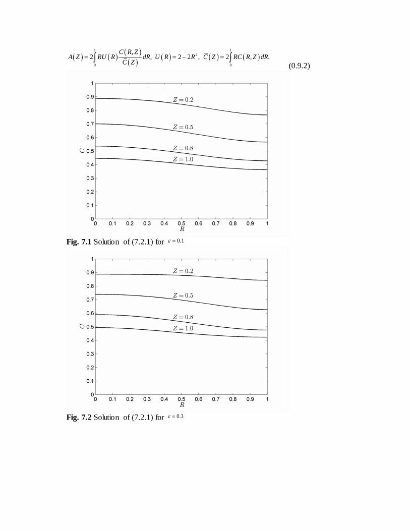
1 12

0 0

,2 , 2 2 , 2 , .

C R ZA Z RU R dR U R R C Z RC R Z dR

C Z= = − =∫ ∫

(0.9.2)

Fig. 7.1 Solution of (7.2.1) for 0.1ε =

Fig. 7.2 Solution of (7.2.1) for 0.3ε =

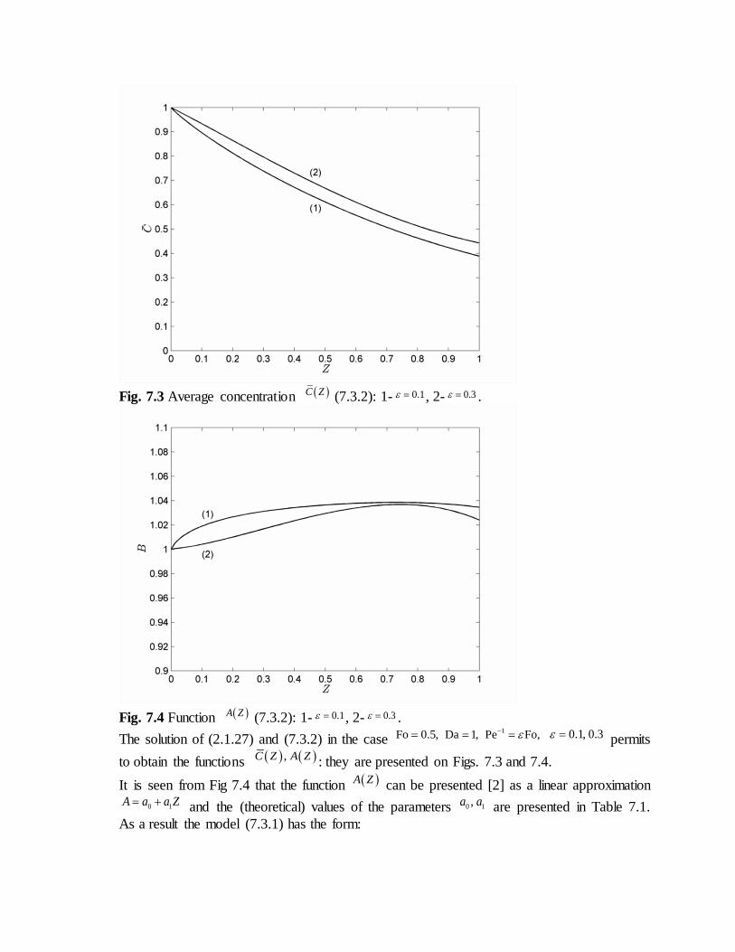
Fig. 7.3 Average concentration ( )C Z (7.3.2): 1- 0.1ε = , 2- 0.3ε = .

Fig. 7.4 Function ( )A Z (7.3.2): 1- 0.1ε = , 2- 0.3ε = . The solution of (2.1.27) and (7.3.2) in the case

1Fo 0.5, Da 1, Pe Fo,ε−= = = 0.1, 0.3ε = permits to obtain the functions ( ) ( ),C Z A Z : they are presented on Figs. 7.3 and 7.4. It is seen from Fig 7.4 that the function ( )A Z can be presented [2] as a linear approximation

0 1A a a Z= + and the (theoretical) values of the parameters 0 1,a a are presented in Table 7.1. As a result the model (7.3.1) has the form:

( )

( )

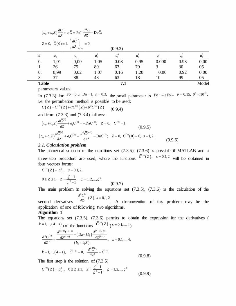
21

0 1 1 2

0

Pe Da ;

Z 0, 0 1, 0. Z

dC d Ca a Z a C CdZ dZ

dCCdZ

−

=

+ + = −

= ≡ ≡

(0.9.3)

Table 7.1 Model parameters values In (7.3.3) for Fo 0.5, Da 1, 0.3,ε= = = the small parameter is 1Pe Foε− = =

3 20.15, 10 ,θ θ −= < i.e. the perturbation method is possible to be used:

( ) ( ) ( ) ( ) ( ) ( ) ( )0 1 22C Z C Z C Z C Zθ θ= + + (0.9.4) and from (7.3.3) and (7.3.4) follows:

( )

( )( ) ( ) ( )

00 0 0

0 1 1 Da ; 0, 1.dCa a Z a C C Z CdZ

+ + = − = = (0.9.5)

( )( )

( )( )

( ) ( ) ( )12

0 1 1 2 Da ; 0, 0 0, 1,2.s s

s s sdC d Ca a Z a C C Z C sdZ dZ

−

+ + = − = = = (0.9.6)

3.1. Calculation problem The numerical solution of the equations set (7.3.5), (7.3.6) is possible if MATLAB and a

three-step procedure are used, where the functions ( ) ( ) , 0,1, 2sC Z s = will be obtained in

four vectors forms:

( ) ( )0

0

, 0,1, 2,

10 1, , 1, 2,..., .1

s sC Z a s

Z Z

ζ

ζ ζ ζζ

= =

−≤ ≤ = =

− (0.9.7) The main problem in solving the equations set (7.3.5), (7.3.6) is the calculation of the

second derivatives

( )

( )2

2 , 0,1, 2sd C Z s

dZ=

. A circumvention of this problem may be the application of one of following two algorithms. Algorithm 1 The equations set (7.3.5), (7.3.6) permits to obtain the expression for the derivatives (

( )1,..., 4k s= − ) of the functions ( ) ( )sC Z ( 0,1,..., 4s = ):

( )

( )

( ) ( )( ) ( )

( )

( )

( )( )

( )

1 1(s 1)

11 1

0 1

0( 1)

0

Da, 0,1,..., 4,

1,..., 4 , 0, .

k k s

sk k k

k

ss

d C d Ckbd C dZ dZ sb b ZdZ

d Ck s C CdZ

+ −−

+ −

−

− += =

+

= − = = (0.9.8)

The first step is the solution of (7.3.5)

( ) ( )0 0 0

0

1, 0 1, , 1, 2,...,1

C Z a Z Zζζ ζ ζζ−

= ≤ ≤ = =− (0.9.9)

ε 0a 1a 00a

01a

10a

11a

20a

21a

0.1

1,0126

0,0075

1.0589

0.0863

0.9579

0.0003

0.9330

0.0005

0.3

0,9937

0,0288

1.0743

0.1663

1.2018

−0.0010

0.9299

0.0005

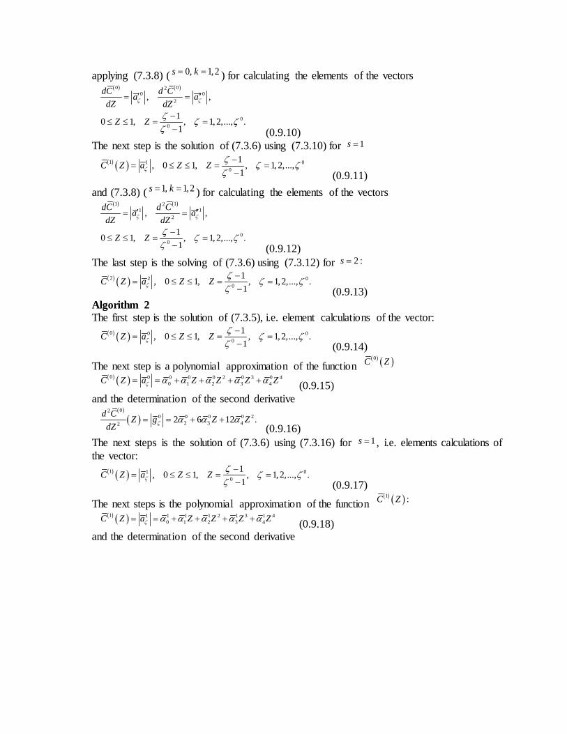
applying (7.3.8) ( 0, 1,2s k= = ) for calculating the elements of the vectors

( ) ( )0 020 0

2

00

, ,

10 1, , 1, 2,..., .1

dC d Ca adZ dZ

Z Z

ζ ζ

ζ ζ ζζ

′ ′′= =

−≤ ≤ = =

− (0.9.10) The next step is the solution of (7.3.6) using (7.3.10) for 1s =

( ) ( )1 1 0

0

1, 0 1, , 1, 2,...,1

C Z a Z Zζζ ζ ζζ−

= ≤ ≤ = =− (0.9.11)

and (7.3.8) ( 1, 1,2s k= = ) for calculating the elements of the vectors

( ) ( )1 121 1

2

00

, ,

10 1, , 1, 2,..., .1

dC d Ca adZ dZ

Z Z

ζ ζ

ζ ζ ζζ

′ ′′= =

−≤ ≤ = =

− (0.9.12) The last step is the solving of (7.3.6) using (7.3.12) for 2 :s =

( ) ( )2 2 0

0

1, 0 1, , 1, 2,..., .1

C Z a Z Zζζ ζ ζζ−

= ≤ ≤ = =− (0.9.13)

Algorithm 2 The first step is the solution of (7.3.5), i.e. element calculations of the vector:

( ) ( )0 0 0

0

1, 0 1, , 1, 2,..., .1

C Z a Z Zζζ ζ ζζ−

= ≤ ≤ = =− (0.9.14)

The next step is a polynomial approximation of the function ( ) ( )0C Z

( ) ( )0 0 0 0 0 2 0 3 0 4

0 1 2 3 4C Z a Z Z Z Zζ a a a a a= = + + + + (0.9.15) and the determination of the second derivative

( )

( )02

0 0 0 0 22 3 42 2 6 12 .d C Z g Z Z

dZ ζ a a a= = + + (0.9.16)

The next steps is the solution of (7.3.6) using (7.3.16) for 1s = , i.e. elements calculations of the vector:

( ) ( )1 1 0

0

1, 0 1, , 1, 2,..., .1

C Z a Z Zζζ ζ ζζ−

= ≤ ≤ = =− (0.9.17)

The next steps is the polynomial approximation of the function ( ) ( )1 :C Z

( ) ( )1 1 1 1 1 2 1 3 1 4

0 1 2 3 4C Z a Z Z Z Zζ a a a a a= = + + + + (0.9.18) and the determination of the second derivative

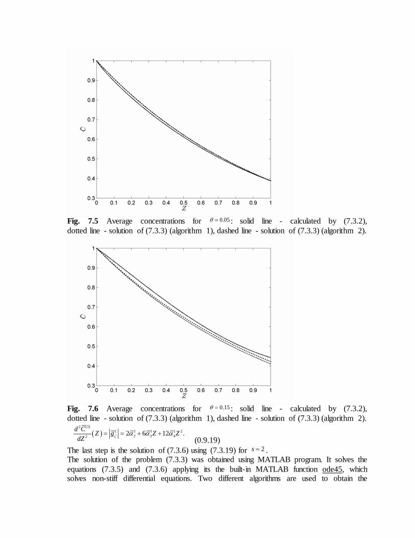
Fig. 7.5 Average concentrations for 0.05θ = : solid line - calculated by (7.3.2), dotted line - solution of (7.3.3) (algorithm 1), dashed line - solution of (7.3.3) (algorithm 2).

Fig. 7.6 Average concentrations for 0.15θ = : solid line - calculated by (7.3.2), dotted line - solution of (7.3.3) (algorithm 1), dashed line - solution of (7.3.3) (algorithm 2).

( )

( )12

1 1 1 1 22 3 42 2 6 12 .d C Z g Z Z

dZ ζ a a a= = + + (0.9.19)

The last step is the solution of (7.3.6) using (7.3.19) for 2s = . The solution of the problem (7.3.3) was obtained using MATLAB program. It solves the equations (7.3.5) and (7.3.6) applying its the built-in MATLAB function ode45, which solves non-stiff differential equations. Two different algorithms are used to obtain the

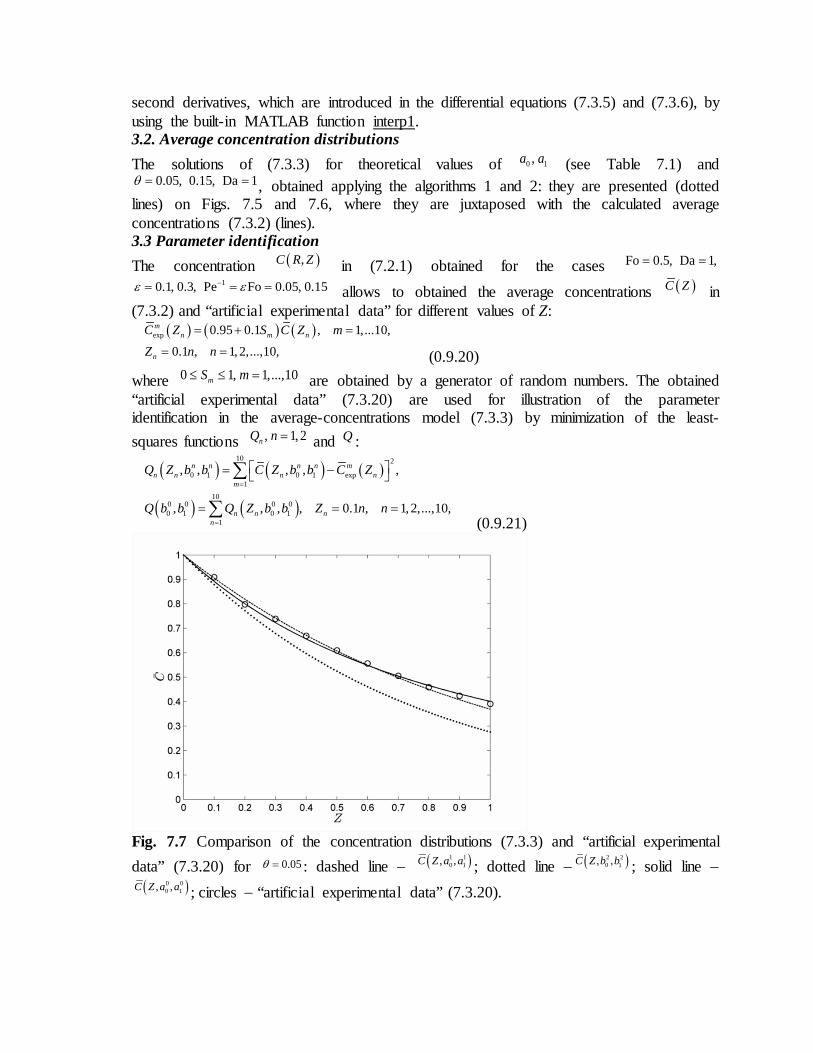
second derivatives, which are introduced in the differential equations (7.3.5) and (7.3.6), by using the built-in MATLAB function interp1. 3.2. Average concentration distributions The solutions of (7.3.3) for theoretical values of 0 1,a a (see Table 7.1) and

0.05, 0.15, Da 1θ = = , obtained applying the algorithms 1 and 2: they are presented (dotted lines) on Figs. 7.5 and 7.6, where they are juxtaposed with the calculated average concentrations (7.3.2) (lines). 3.3 Parameter identification The concentration ( ),C R Z in (7.2.1) obtained for the cases Fo 0.5, Da 1,= =

10.1, 0.3, Pe Fo 0.05, 0.15ε ε−= = = allows to obtained the average concentrations ( )C Z in (7.3.2) and “artificial experimental data” for different values of Z:

( ) ( ) ( )exp 0.95 0.1 , 1,...10,

0.1 , 1,2,...,10,

mn m n

n

C Z S C Z mZ n n

= + =

= = (0.9.20) where 0 1, 1,...,10mS m≤ ≤ = are obtained by a generator of random numbers. The obtained “artificial experimental data” (7.3.20) are used for illustration of the parameter identification in the average-concentrations model (7.3.3) by minimization of the least-squares functions , 1, 2nQ n = and Q :

( ) ( ) ( )

( ) ( )

10 2

0 1 0 1 exp1

100 0 0 00 1 0 1

1

, , , , ,

, , , , 0.1 , 1, 2,...,10,

n n n n mn n n n

m

n n nn

Q Z b b C Z b b C Z

Q b b Q Z b b Z n n

=

=

= −

= = =

∑

∑ (0.9.21)

Fig. 7.7 Comparison of the concentration distributions (7.3.3) and “artificial experimental data” (7.3.20) for 0.05θ = : dashed line − ( )1 1

0 1, ,C Z a a ; dotted line − ( )2 20 1, ,C Z b b ; solid line −

( )0 00 1, ,C Z a a ; circles − “artificial experimental data” (7.3.20).

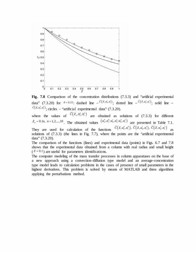
Fig. 7.8 Comparison of the concentration distributions (7.3.3) and “artificial experimental data” (7.3.20) for 0.15θ = : dashed line − ( )1 1

0 1, ,C Z a a ; dotted line − ( )2 20 1, ,C Z a a ; solid line −

( )0 00 1, ,C Z a a ; circles − “artificial experimental data” (7.3.20).

where the values of ( )0 1, ,n nnC Z b b are obtained as solutions of (7.3.3) for different

0.1 , 1,2,...,10nZ n n= = . The obtained values ( )0 0 1 1 2 20 1 0 1 0 1, ; , ; ,a a a a a a are presented in Table 7.1.

They are used for calculation of the functions ( ) ( ) ( )0 0 1 1 2 20 1 0 1 0 1, , , , , , , ,C Z a a C Z a a C Z a a as

solutions of (7.3.3) (the lines in Fig. 7.7), where the points are the “artificial experimental data” (7.3.20). The comparison of the functions (lines) and experimental data (points) in Figs. 6.7 and 7.8 shows that the experimental data obtained from a column with real radius and small height ( 0.1Z = ) are useful for parameters identifications. The computer modeling of the mass transfer processes in column apparatuses on the base of a new approach using a convection–diffusion type model and an average-concentration type model leads to calculation problems in the cases of presence of small parameters in the highest derivatives. This problem is solved by means of MATLAB and three algorithms applying the perturbations method.