Embed Size (px)
Citation preview

Modeling and predicting of different stock markets with
GARCH model Author:Wei Jiang
Supervisor: Lars Forsberg
2012/6/1
Master Thesis in Statistics Department of Statistics
Uppsala University Sweden
1
Modeling and predicting of different stock markets with
GARCH model
June, 2012
Abstract
This paper is mainly talking about several volatility models and its ability to predict and capture the distinctive characteristics of conditional variance about the empirical financial data. In my paper, I choose basic GARCH model and two important models of the GARCH family which are E-GARCH model and GJR-GARCH model to estimate. At the same time, in order to acquire the forecasting performance, I consider to use two different distributions on error term: normal distribution and student-t distribution. Finally, for each set of empirical stock price, I could get the best model to predict the conditional variance of the stock return based on comparing the Root Mean Square Error (RMSE)’s values of different models. Here, I select several main global stock markets indexes: NASDAQ’s daily index (America), Standard and Poor’s 500 daily index (America), FTSE100 daily index (UK), HANG SENG daily index (Hong Kong) and NIKKEI daily index (Japan). Key words: conditional variance; GARCH and GARCH family models; error distribution; Root Mean Square Error (RMSE)

2
Contents
1 Introduction ………………………………………………………………………… 4 1.1 Background ………………………………………………………………………… 4 1.2 Literature review …………………………………………………………………… 4
2 Methodology ……………………………………………………………………… 5 2.1 ARCH model ……………………………………………………………………… 5 2.2 Generalized-ARCH model (GARCH) ………………………………………………… 6 2.3 Exponential GARCH (EGARCH) model ……………………………………………… 7 2.4 GJR-GARCH model ………………………………………………………………… 8 2.5 Distribution of the error term ……………………………………………………… 9
2.5.1 Normal distribution ………………………………………………………… 9 2.5.2 Student-t distribution ………………………………………………………… 9
2.6 Root Mean Square Error (RMSE) ……………………………………………………10
3 Data ………………………………………………………………………………… 10 3.1 Data description …………………………………………………………………… 10
3.1.1 NASDAQ Stock Market Daily Closing Price Index …………………………… 10 3.1.2 Standard & Poor 500 Stock Market Daily Closing Price Index ……………… 11 3.1.3 FTSE100 Stock Market Daily Closing Price Index …………………………… 11 3.1.4 HANG SENG Stock Market Daily Closing Price Index ……………………… 11 3.1.5 NIKKEI Stock Market Daily Closing Price Index ……………………………… 11
3.2 Data analysis …………………………………………………………………… 11 3.2.1 NASDAQ analysis …………………………………………………………… 12 3.2.2 Standard & Poor 500 analysis ……………………………………………… 13 3.2.3 FTSE100 analysis …………………………………………………………… 13 3.2.4 HANG SENG analysis ………………………………………………………… 14 3.2.5 NIKKEI analysis ……………………………………………………………… 15
4 Results ………………………………………………………………………………17 4.1 Application in NASDAQ daily return ……………………………………………… 17
4.1.1 Selection of ARMA (p, q) model …………………………………………… 17 4.1.2 Result of GARCH model and GARCH family model for NASDAQ …………… 18
4.2 Application in Standard &Poor 500 daily return ………………………………… 20 4.2.1 Selection of ARMA (p, q) model …………………………………………… 20 4.2.2 Result of GARCH model and GARCH family model for Standard & Poor
500 ………………………………………………………………………… 20 4.3 Application in FTSE100 daily return ……………………………………………… 22
4.3.1 Selection of ARMA (p, q) model …………………………………………… 22 4.3.2 Result of GARCH model and GARCH family model for FTSE100 …………… 23
4.4 Application in NIKKEI daily return ……………………………………………… 25 4.4.1 Selection of ARMA (p, q) model …………………………………………… 25
3
4.4.2 Result of GARCH model and GARCH family model for NIKKEI ……………… 25 4.5 Application in HANG SENG daily return ………………………………………… 27
4.5.1 Selection of ARMA (p, q) model ………………………………………… 27 4.5.2 Result of GARCH model and GARCH family model for HANG
SENG ……………………………………………………………………………28 4.6 ARCH-LM Test …………………………………………………………………… 29 4.7 Out-of-sample Forecast ………………………………………………………… 30
5 Conclusion …………………………………………………………………………32
6 Reference ………………………………………………………………………… 33 6.1 article resource……………………………………………………………………… 33 6.2 websites resource ………………………………………………………………… 34
7 Appendix ………………………………………………………………………… 35 7.1 Appendix A ………………………………………………………………………… 35 7.2 Appendix B ………………………………………………………………………… 36

4
1. Introduction
This article is an application about the GARCH and extension GARCH model. So it’s mainly focused on the selection of the appropriate model to estimate the financial volatility data and using this model to forecast the conditional variance of the stock return. Full text is organized as follows. In the section 1, it includes background and the literature review. Section2 introduces the classic ARCH/GARCH model and the extension GARCH model, error distribution and the method of Root Mean Square Error. The data description and analysis are presented in Section 3. Section 4 considers the result of all models, ARCH-LM test and the out-of sample forecast, and Section 5 points out the conclusion. The reference and the appendix could be found at the end.
1.1 Background Econometricians are always committed to fitting models to various kinds of data, both cross-sectional data and time series data, also including some financial volatility data, such as stock price, exchange-rate, and gold price and so on. After the detailed research, I am aware of some special characteristics of financial volatility data: long memory, fat tails and excess kurtosis, clustering volatility, leverage effect and spillover effect, these features are introduced by Bollerslev and Mikkelsen (1996). Historically, they often focused their attention on modeling conditional first moments; see e.g. Bollerslev, Engle and Nelson (1994). They set an underlying assumption for these analyses and assure this assumption to be valid, so the assumption is a variation in the error terms is constant for a data set at any time and location. It means the variation in the error terms will not change along with the changes of the time. So this kind of variance is known to be homoscedastic. But this assumption is not always valid in all cases. The error variance might be larger for some special intervals, and smaller for others. Especially for the financial data, this situation is obvious. According to this particular phenomenon, the error term is then said to suffer from heteroscedasticity, which is proposed by Bollerslev (1987). After constantly exploring, some advanced ARCH, GARCH and extension GARCH models are utilized to analysis the financial volatility data including these features.
Enocksson and Skoog (2012).
1.2 Literature review To large extent, Economists have already captured the changes in financial data over a long time. From the paper of Franses and Mcaleer (2002), it can be seen many financial economists are very concerned about how to estimate the volatility of assets’ returns better. They also do much try and explore many researches which made a possible is that almost every price series exhibits the same characteristics, so we have to find some approximate volatility models to fit these features. This was pointed out early by French, Schwert and Stambaugh (1987) and Bollerslev (1987), and is especially clear in some of the surveys of empirical work from Engle’s paper (2002).
5
And next, I will simply summary what they have studied about the volatility models and some achievement which they have got until now. This first model is Autoregressive Conditional Heteroskedasticity (ARCH) which was early introduced in the Engle’s paper (1982), it aimed to capture the conditional variance that is why it became the most popular way of describing the unique feature. Later on, for making this model better, Bollerslev (1986) and Taylor (1986) put forward, independently of each other, a generalization of this model, called Generalized ARCH (GARCH). And this model have been certificated not only to catch volatility clustering but also to contain fat tails from the volatility data. These are common features about the financial data. Even though the GARCH model is already the extension of the ARCH model, it still has some drawbacks. The main point is that the GARCH model is symmetric, so it has a poor performance in reflecting the asymmetry. Because a fact on an interesting feature of financial volatility data
is that bad news seems to have a more significant effect on the fluctuation compared to good ones. In other words, positive and negative information generate different degrees of influence to the changes of financial data. So this asymmetric phenomenon is leverage effect. Considering the stock data, it always exist a strong negative correlation between the current return and the future conditional variance. That is why some advanced GARCH model will be introduced later. Such as exponential-GARCH model, Nelson (1991) and GJR-GARCH model, Glosten, Jangannathan and Runkle (1993), are proposed. Except these models, there still have many other extension GARCH models, such as TGARCH model—threshold ARCH—attributed to Rabemananjara and Zakoian (1993) and Glosten, Jaganathan and Runkle (1993), FIGARCH model—introduced by Baillie, Bollerslev and Mikkelsen (1996) IGARCH model—proposed by Engle and Bollerslev (1986) and so on.
2. Methodology
2.1 ARCH model
ARCH (Auto-regressive Conditional Heteoskedastic Model) is the first and the basic model in stochastic variance modeling and is proposed by Engle (1982). The key point of this model is that it already changes the assumption of the variation in the error terms from
constant Var(ε ) = σ to be a random sequence which depended on the past residuals ({ε … ε }) . That is to say, this model has changed the restriction from
homoscedastic to be heteroscedasticity. This breakthrough is explained by Baillie and Bollerslev (1989). And this is an accurate change to reflect the volatility data’s features. Let ε as a random variable that has a mean and a variance conditionally on the information set Ι , The ARCH model of ε has the following properties. Come from Teräsvirta (2006). First,
E(ε | Ι ) = 0.
And second, conditional variance

6
σ = E(ε | Ι ),
is a positive valued parametric function of Ι . The sequence {ε } may be observed directly, or it may be got from the following formula. In the latter case, I can get
ε = y − μ (y ) Where y is observed value, and μ (y ) = E(y | Ι ) is the conditional mean of y given Ι , Engle’s (1982) application was of this type. In what follows, the ε could be
expressed as another way on parametric forms of σ . So, here ε is assumed as follows:
ε = z σ Where {z } is a sequence of independent, identically distributed (iid) random variables with zero mean and unit variance. This implied:
ε ~D(0, σ ),
So the ARCH model of order q is like this: σ = α + α ε +. . . +α ε = α + ∑ α ε (1)
Where α > 0, and α ≥ 0, i > 0. To assure {σ } is asymptotically stationary random sequence, I can assume that α +. . . +α < 1. This is the ARCH model.
With the generation of ARCH model, it already can explain many problems in many fields, for instance, interest rates, exchange rates and trade option and stock index returns. Bollerslev, Chou and Kroner (1992) already used these models to achieve a variety of applications in their survey. It’s different between forecasting the conditional variance of these series and forecasting the conditional mean of them because the conditional variance cannot be observed. So how to measure the conditional variance should be considered from Andersen and Bollerslev (1998).
2.2 Generalized-ARCH model (GARCH)
Because of some drawbacks and limitation on ARCH model, it has been substituted by the so-called generalized ARCH (GARCH) model that Bollerslev (1986) and Taylor (1986) proposed independently of each other. Based on the ARCH model has been raised, it adds the lagged conditional variance term (σ ) as a new term in the GARCH model. The
improved ARCH model (GARCH model) also reduces the number of estimated parameters. In this model, the conditional variance is still a linear function of its own lags and error terms, it has the following form:
7
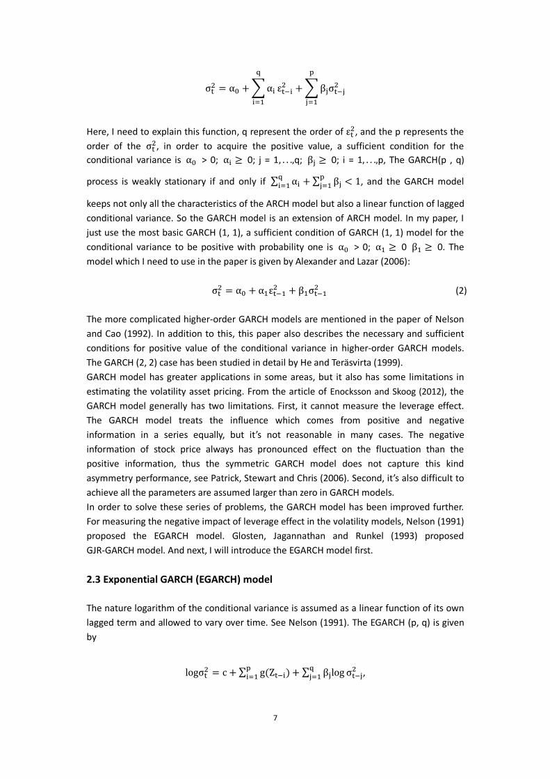
σ = α + α ε + β σ
Here, I need to explain this function, q represent the order of ε , and the p represents the order of the σ , in order to acquire the positive value, a sufficient condition for the conditional variance is α > 0; α ≥ 0; j = 1, . . .,q; β ≥ 0; i = 1, . . .,p, The GARCH(p , q)
process is weakly stationary if and only if ∑ α + ∑ β < 1, and the GARCH model
keeps not only all the characteristics of the ARCH model but also a linear function of lagged conditional variance. So the GARCH model is an extension of ARCH model. In my paper, I just use the most basic GARCH (1, 1), a sufficient condition of GARCH (1, 1) model for the conditional variance to be positive with probability one is α > 0; α ≥ 0 β ≥ 0. The model which I need to use in the paper is given by Alexander and Lazar (2006):
σ = α + α ε + β σ (2) The more complicated higher-order GARCH models are mentioned in the paper of Nelson and Cao (1992). In addition to this, this paper also describes the necessary and sufficient conditions for positive value of the conditional variance in higher-order GARCH models. The GARCH (2, 2) case has been studied in detail by He and Teräsvirta (1999). GARCH model has greater applications in some areas, but it also has some limitations in estimating the volatility asset pricing. From the article of Enocksson and Skoog (2012), the GARCH model generally has two limitations. First, it cannot measure the leverage effect. The GARCH model treats the influence which comes from positive and negative information in a series equally, but it’s not reasonable in many cases. The negative information of stock price always has pronounced effect on the fluctuation than the positive information, thus the symmetric GARCH model does not capture this kind asymmetry performance, see Patrick, Stewart and Chris (2006). Second, it’s also difficult to achieve all the parameters are assumed larger than zero in GARCH models. In order to solve these series of problems, the GARCH model has been improved further. For measuring the negative impact of leverage effect in the volatility models, Nelson (1991) proposed the EGARCH model. Glosten, Jagannathan and Runkel (1993) proposed GJR-GARCH model. And next, I will introduce the EGARCH model first.
2.3 Exponential GARCH (EGARCH) model
The nature logarithm of the conditional variance is assumed as a linear function of its own lagged term and allowed to vary over time. See Nelson (1991). The EGARCH (p, q) is given by
logσ = c + ∑ g(Z ) + ∑ β log σ ,
8
Where, I simplify the
g(Z ) = γ Z + α |Z | − E(|Z |) ,
g(Z ) is a function of both the magnitude and sign of Z , γ Z is sign effect,
α |Z | − E(|Z |) is magnitude effect. σ is the conditional variance, c, γ, α, β are
the coefficients, and I define Z = and the function should be written as:
log(σ ) = c + β log σ + αεσ
− Eεσ
+ γεσ
E(|Z |) =
⎩⎪⎨
⎪⎧ π
2, 푤ℎ푒푛 Z is normal distribution
√νΓ[0.5(ν − 1)]√πΓ(0.5ν)
, 푤ℎ푒푛 Z is student − t distribution�
Here, Z have two different kinds of distributions, normal distribution and student-t distribution. And c, γ, α, β are the parameters, the α parameter represents a magnitude effect or the symmetric effect of the model, the same role as the ‘’ARCH” effect. The parameter β measures conditional variance. The same role as the “GARCH” model. If β is quite large, it will consume a long time to die out under a market crisis and vice versa. See Alexander (2004). The parameter γ reflects the asymmetric performance or leverage effect. So the parameter γ is an outstanding extension from GARCH model to EGARCH model. If γ = 0, which means the model doesn’t exist asymmetric, when γ < 0, which means the negative news generate pronounced effect than the positive news. When γ > 0, it implies the opposite situation that is positive information is more significant than negative information. see Patrick, Stewart and Chris (2006). Here, in the article of Wang, Fawson, Barrett and Mcdonald (2001), they point out E(|Z |) is constant for all i when Z is normal distribution or else when Z is student-t distribution. And in my paper, I just use the EGARCH (1, 1) model which is simplified by
log(σ ) = c + γ ∗ Z + α ∗ |Z | − α ∗ E|Z | + β log(σ ) (3) Another GARCH family’s model is GJR-GARCH model.
2.4 GJR-GARCH model
The GJR-GARCH model, Glosten, Jagannathan and Runkle (1993) proposed, is another model could measure the asymmetry in the GARCH family models. The same, I define the
ε = z σ , where z ~D(0, 1), ε ~D(0, σ ) so the GJR-GARCH model is written by

9
σ = c + β σ + α ε + γ ε I (ε < 0)
Where I is an indicator variable taking the value one if the residual is smaller than zero and the value zero if the residual is not smaller than zero.
I = 1, if ε < 0 0, otherwise
� ,
From this model, it also captures the asymmetric impacts by the sign of the indicator term to reflect different influence between good news and bad news. This is another expression different from the EGARCH model. And the more detail could be acquired from Patrick, Stewart and Chris (2006). The most common GJR-GARCH model is simplified as follows:
σ = c + β σ + α ε + γ ε I (ε < 0) (4)
2.5 Distribution of the error term
The distribution of error term also plays an important role in estimating the volatility model. And in my paper, I mainly introduce two common distributions. One is normal distribution, the other is student-t distribution. The most common application is assumed as standard normal distribution. In some situations, this normal distribution is not good; maybe the error term is fat tail, so normal distribution cannot capture this feature. That is why I choose the student-t distribution as my second choice. So I choose another distribution, student-t distribution, which maybe explains the fat-tailed distribution better. Actually, it still has many other assumptions, but in my paper I just introduce these two distributions as examples. 2.5.1 Normal distribution
The probability density function of Z is given as normal distribution,
f( Z ) =√
exp − ( μ) (5)
where μ is mean and σ is standard deviation. 2.5.2 Student t-distribution
The Conditional density function of Z is student t-distribution and the density function is given by:
10
f( Z ) =ν
ν (ν )(1 +
ν) (ν ) (6)
Where ν is the number of degree of freedom, 2 < ν ≤ ∞, and the Γ is gamma function. When ν → ∞ the student-t distribution nearly equals to the normal distribution. The lower the ν, the fatter the tails. So the student-t distribution maybe reflects the fat-tail of the volatility index more exactly.
2.6 Root Mean Square Error (RMSE)
Many methods could be chose to test model is better or not, such as MSE, RMSE from Lars and Eric (2007). This paper uses the RMSE as a test to measure GARCH models. The Root Mean Square Error (RMSE) (also called the root mean square deviation, RMSD) is a frequently measure of the difference between estimated values predicted by a model and the true values actually observed. These individual differences are also called residuals, and the RMSE aims to aggregate all these residuals together as a standard of predictive power. The criterion is the smaller value of the RMSE, the better the predicting ability of the model. And in my thesis, I use this method to decide which model has the best forecasting performance from GARCH and GARCH family models. The RMSE of a model prediction with
respect to the estimated variable r is defined as the square root of the mean squared error (http://en.wikipedia.org/wiki/Root-mean-square_deviation):
RMSE = ∑ (7)
where r is observed values and σ is the predicted value of conditional variance at time i, n is the number of forecasts.
3. Data
3.1 Data description
3.1.1 NASDAQ Stock Market Daily Closing Price Index
The first data I used is NASDAQ daily index. The NASDAQ Stock Market, also known as simply the NASDAQ, it’s an American stock exchange. "NASDAQ" originally represented “National Association of Securities Dealers Automated Quotations". Except the New York Stock Exchange, it already becomes the second-largest stock exchange in the world’s stock market. In addition to this, the NASDAQ has large trading volume than any other electronic stock exchange market, because NASDAQ daily closing price index is very significant and representative, so that is why I choose the NASDAQ daily closing price index as my data. The data I chose from Yahoo Finance between 2007-1-3 and 2011-12-30. (http://finance.yahoo.com/q/hp?s=%5EIXIC+Historical+Prices).
11
3.1.2 Standard & Poor 500 Stock Market Daily Closing Price Index
The S&P 500 stands for Standard & Poor 500 and is a free-float capitalization-Iighted index published since 1957 and it includes 500 large-cap common stocks actively traded in the United States. Comparing with the Dow Jones Industrial Average, S&P500 has more companies, so the risk is more dispersed and it could reflect the changes in the market broader. Based on these features, S&P 500 is generally considered as the standard of ideal stock index future contracts. I choose Standard & Poor 500 daily close index from Yahoo Finance between 2007-1-3 and 2011-12-30. (http://finance.yahoo.com/q/hp?s=%5EGSPC+Historical+Prices). 3.1.3 FTSE100 Stock Market Daily Closing Price Index
The FTSE 100 Index, also known as London's FTSE 100 index (the Financial Times Stock Exchange 100 Index), FTSE, is a share index of the stocks of the largest 100 companies listed on the London Stock Exchange. This index is a barometer of the UK economy and one of the most important stock indexes in Europe, including the FTSE 250 index and the combination of the FTSE350 index. It is the most widely used of the FTSE Group's indices, and is frequently reported (e.g. on UK news bulletins) as a measure of business prosperity. I choose FTSE100 daily close index from Yahoo Finance between 2007-1-2 and 2011-12-30. (http://finance.yahoo.com/q/hp?s=%5EFTSE+Historical+Prices). 3.1.4 HANG SENG Stock Market Daily Closing Price Index
The Hang Seng Index (abbreviated: HSI, Chinese) is a free float-adjusted market capitalization-Iighted stock market index in Hong Kong. The Hang Seng Index is an important indicator of the Hong Kong stock market price index calculated by the market value of the number of constituent stocks (blue chips), representing 70% of all listed companies on the Hong Kong Stock Exchange. It is used to record and monitor daily changes of the largest companies of the Hong Kong stock market and is a most influential stock index that reflects the increase trend of the Hong Kong stock market price. I choose HANG SENG daily close index from Yahoo Finance between 2007-1-2 and 2011-12-30.
(http://finance.yahoo.com/q/hp?s=%5EHSI+Historical+Prices).
3.1.5 NIKKEI Stock Market Daily Closing Price Index
The Nikkei (Nikkei heikin kabuki, Nikkei 225), more commonly called the Nikkei, the Nikkei index, or the Nikkei Stock Average, is a stock market index for the Tokyo Stock Exchange (TSE). It has been calculated daily by the Nihon Keizai Shimbun (Nikkei), Tokyo Stock Exchange 225 varieties of the stock index. This index with longer duration and good comparability has already become the most common and reliable indicators to study the changes in the Japanese’s stock market. NIKKEI is the widest index which has been quoted as the daily index by media. I choose NIKKEI 225 daily close index from Yahoo Finance between 2007-1-4 and 2011-12-30.
12
(http://finance.yahoo.com/q/hp?s=%5EN225+Historical+Prices).
3.2 Data analysis
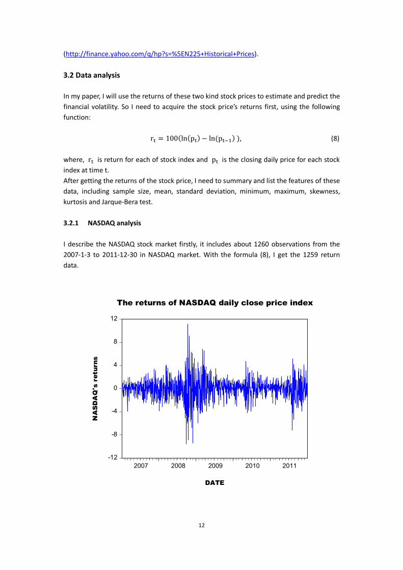
In my paper, I will use the returns of these two kind stock prices to estimate and predict the financial volatility. So I need to acquire the stock price’s returns first, using the following function: r = 100(ln(p ) − ln(p ) ), (8) where, r is return for each of stock index and p is the closing daily price for each stock index at time t. After getting the returns of the stock price, I need to summary and list the features of these data, including sample size, mean, standard deviation, minimum, maximum, skewness, kurtosis and Jarque-Bera test. 3.2.1 NASDAQ analysis
I describe the NASDAQ stock market firstly, it includes about 1260 observations from the 2007-1-3 to 2011-12-30 in NASDAQ market. With the formula (8), I get the 1259 return data.
-12
-8
-4
0
4
8
12
2007 2008 2009 2010 2011
The returns of NASDAQ daily close price index
NA
SD
AQ
's r
etur
ns
DATE
13
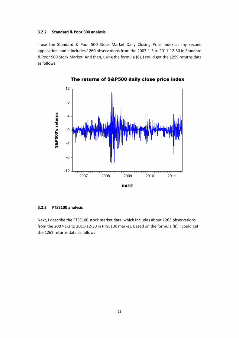
3.2.2 Standard & Poor 500 analysis
I use the Standard & Poor 500 Stock Market Daily Closing Price Index as my second application, and it includes 1260 observations from the 2007-1-3 to 2011-12-30 in Standard & Poor 500 Stock Market. And then, using the formula (8), I could get the 1259 returns data as follows:
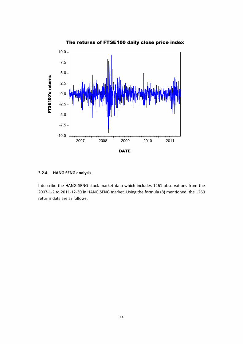
3.2.3 FTSE100 analysis
Next, I describe the FTSE100 stock market data, which includes about 1263 observations from the 2007-1-2 to 2011-12-30 in FTSE100 market. Based on the formula (8), I could get the 1262 returns data as follows:
-12
-8
-4
0
4
8
12
2007 2008 2009 2010 2011
The returns of S&P500 daily close price index
DATE
S&
P50
0's
retu
rns
14
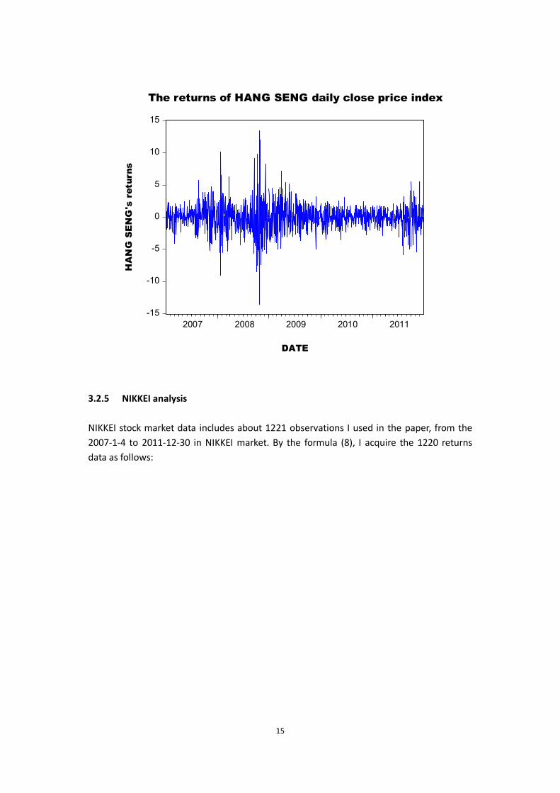
3.2.4 HANG SENG analysis
I describe the HANG SENG stock market data which includes 1261 observations from the 2007-1-2 to 2011-12-30 in HANG SENG market. Using the formula (8) mentioned, the 1260 returns data are as follows:
-10.0
-7.5
-5.0
-2.5
0.0
2.5
5.0
7.5
10.0
2007 2008 2009 2010 2011
The returns of FTSE100 daily close price indexFT
SE
100'
s re
turn
s
DATE
15
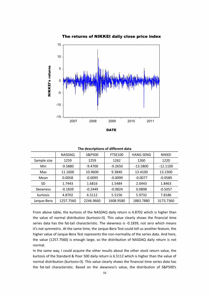
3.2.5 NIKKEI analysis
NIKKEI stock market data includes about 1221 observations I used in the paper, from the 2007-1-4 to 2011-12-30 in NIKKEI market. By the formula (8), I acquire the 1220 returns data as follows:
-15
-10
-5
0
5
10
15
2007 2008 2009 2010 2011
The returns of HANG SENG daily close price index
HA
NG
SE
NG
's r
etur
ns
DATE
16
The descriptions of different data
NASDAQ S&P500 FTSE100 HANG SENG NIKKEI
Sample size 1259 1259 1262 1260 1220
Min -9.5880 -9.4700 -9.2650 -13.5800 -12.1100
Max 11.1600 10.9600 9.3840 13.4100 13.2300
Mean 0.0058 -0.0095 -0.0099 -0.0077 -0.0589
SD 1.7443 1.6816 1.5484 2.0443 1.8463
Skewness -0.1839 -0.2449 -0.0824 0.0898 -0.5057
kurtosis 4.8702 6.5112 5.5156 5.9732 7.8186
Jarque-Bera 1257.7560 2246.9660 1608.9580 1883.7880 3173.7360
From above table, the kurtosis of the NASDAQ daily return is 4.8702 which is higher than the value of normal distribution (kurtosis=3). This value clearly shows the financial time series data has the fat-tail characteristic. The skewness is -0.1839, not zero which means it’s not symmetric. At the same time, the Jarque-Bera Test could tell us another feature, the higher value of Jarque-Bera Test represents the non-normality of the series data. And here, the value (1257.7560) is enough large, so the distribution of NASDAQ daily return is not normal. In the same way, I could acquire the other results about the other stock return value, the kurtosis of the Standard & Poor 500 daily return is 6.5112 which is higher than the value of normal distribution (kurtosis=3). This value clearly shows the financial time series data has the fat-tail characteristic. Based on the skewness’s value, the distribution of S&P500’s
-15
-10
-5
0
5
10
15
2007 2008 2009 2010 2011
The returns of NIKKEI daliy close price index
NIK
KE
I's
retu
rns
DATE

17
return value is asymmetric. At the same time, the Jarque-Bera Test could tell us it’s non-normality of the series data, because the value (2246.9660) is enough large, so the distribution of Standard & Poor 500 daily return is not normal. And the kurtosis of another three daily return values (FTSE100, HANG SENG and NIKKEI) are 5.5156, 5.9732 and 7.8186 which are all higher than the value of normal distribution (kurtosis=3). This value clearly shows the financial time series data has the fat-tail characteristic. And these return values are also non-normality of the series data. Because of the Jarque-Bera’s values (1608.9580, 1883.7880 and 3173.7360) are enough large, so the distributions of daily return about FTSE100, HANG SENG and NIKKEI are not normal. After describing all of five stock market returns, I do the following Box-Ljung test, this test could help us to check if the ARCH effect is existed in the returns or not, the null hypothesis is that the returns data doesn’t exist the ARCH effect, while the alternative hypothesis is opposite. See Forsberg and Bollerslev (2002).
The Box-Ljung test results of different market’s returns
Box-Ljung test
(for returns)
NASDAQ S&P500 FTSE100 HANG SENG NIKKEI
test value 12.8669 20.4826 2.2105 2.4674 2.1696
p-value 0.0003 0.0000 0.0137 0.0116 0.0141
The p-values of different markets’ returns have been show form this table. By the assumption of 5% significance level, all of the results are significant. So the null hypothesis has to be rejected, which means all different markets’ returns exist the ARCH effect. Next I use the ARCH/GARCH model to analysis the different markets’ returns. After modeling with ARCH/GARCH model, the ARCH effect should be eliminated if the ARCH/GARCH model is good to estimate the returns. Finally, the ARCH effect after estimation should be tested again. At that time, the ARCH effect should not be existed any more.
4. Result
In this part, I will separately utilize GARCH model and GARCH family models with different distributions of error term to estimate and forecast the financial volatility using the daily stock return from NASDAQ market index, Standard & Poor 500 daily index, FTSE100 daily index, HANG SENG daily index and NIKKEI daily index. And then compare the results of all the models and choose which model has the best performance to forecast the financial volatility by calculating the RMSE.
4.1 Application in NASDAQ daily return
4.1.1 Selection of ARMA (p, q) model First step is selection of suitable ARMA (p, q) model for NASDAQ daily return. For choosing the exactly parameter p and q to fit the ARMA model, I could roughly get them by observing autocorrelation and partial autocorrelation. According to comparing the value of
18
AIC and BIC, the best one could be picked up. Many models have been tried, such as AR (1), MA (1), ARMA (1, 1) and so on. Finally, I choose p=0, q=1 because the MA (1) has the smallest AIC and BIC of all the models. So I select the MA (1) model finally. From the following function:
r = θ + θ e + e
The estimated parameters are θ = −1e − 04, θ = −0.1461, And then, calculate and take e = r − (θ + θ e ), after that estimate GARCH model on e .
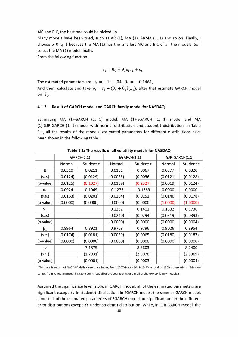
4.1.2 Result of GARCH model and GARCH family model for NASDAQ Estimating MA (1)-GARCH (1, 1) model, MA (1)-EGARCH (1, 1) model and MA (1)-GJR-GARCH (1, 1) model with normal distribution and student-t distribution, In Table 1.1, all the results of the models’ estimated parameters for different distributions have been shown in the following table.
Table 1.1: The results of all volatility models for NASDAQ
GARCH(1,1) EGARCH(1,1) GJR-GARCH(1,1)
Normal Student-t Normal Student-t Normal Student-t
Ω 0.0310 0.0211 0.0161 0.0067 0.0377 0.0320
(s.e.) (0.0124) (0.0129) (0.0065) (0.0056) (0.0121) (0.0128)
(p-value) (0.0125) (0.1027) (0.0139) (0.2327) (0.0019) (0.0124)
α 0.0924 0.1069 -0.1275 -0.1369 0.0000 0.0000
(s.e.) (0.0163) (0.0201) (0.0204) (0.0251) (0.0146) (0.0178)
(p-value) (0.0000) (0.0000) (0.0000) (0.0000) (1.0000) (1.0000)
γ 0.1232 0.1411 0.1532 0.1736
(s.e.) (0.0240) (0.0294) (0.0319) (0.0393)
(p-value) (0.0000) (0.0000) (0.0000) (0.0004)
β 0.8964 0.8921 0.9768 0.9796 0.9026 0.8954
(s.e.) (0.0174) (0.0181) (0.0059) (0.0065) (0.0180) (0.0187)
(p-value) (0.0000) (0.0000) (0.0000) (0.0000) (0.0000) (0.0000)
ν 7.1875 8.3603 8.2400
(s.e.) (1.7931) (2.3078) (2.3369)
(p-value) (0.0001) (0.0003) (0.0004)
(This data is return of NASDAQ daily close price index, from 2007-1-3 to 2011-12-30, a total of 1259 observations. this data
comes from yahoo finance. This table points out all of the coefficients under all of the GARCH family models.)
Assumed the significance level is 5%, in GARCH model, all of the estimated parameters are significant except Ω in student-t distribution. In EGARCH model, the same as GARCH model,
almost all of the estimated parameters of EGARCH model are significant under the different error distributions except Ω under student-t distribution. While, in GJR-GARCH model, the
19
estimation results of α are very bad, α is the coefficient of ε term, and here the
p-value of α is very large, which represents the coefficient of ε is not significant and the
term of ε (ARCH term) has no effect in interpretation of σ .
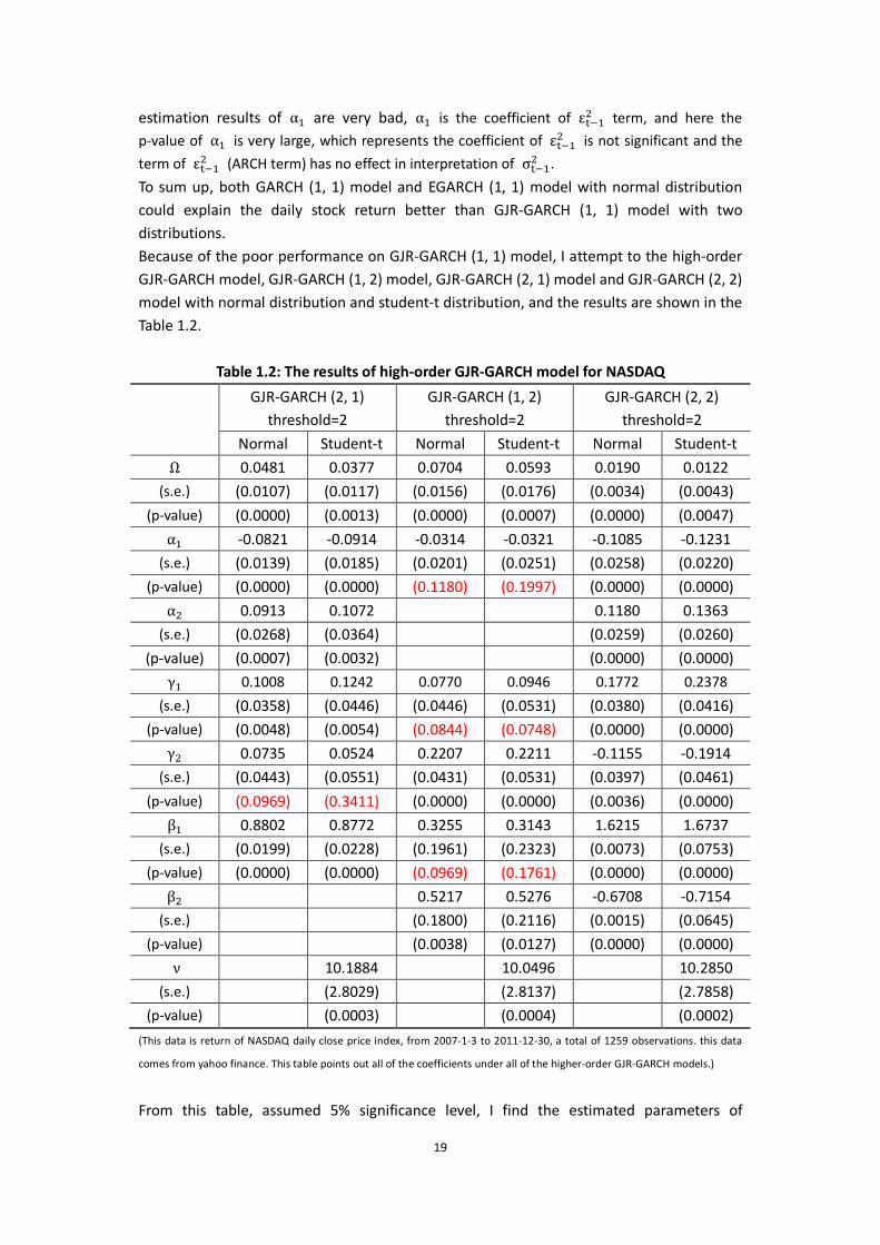
To sum up, both GARCH (1, 1) model and EGARCH (1, 1) model with normal distribution could explain the daily stock return better than GJR-GARCH (1, 1) model with two distributions. Because of the poor performance on GJR-GARCH (1, 1) model, I attempt to the high-order GJR-GARCH model, GJR-GARCH (1, 2) model, GJR-GARCH (2, 1) model and GJR-GARCH (2, 2) model with normal distribution and student-t distribution, and the results are shown in the Table 1.2.
Table 1.2: The results of high-order GJR-GARCH model for NASDAQ
GJR-GARCH (2, 1) threshold=2
GJR-GARCH (1, 2) threshold=2
GJR-GARCH (2, 2) threshold=2
Normal Student-t Normal Student-t Normal Student-t
Ω 0.0481 0.0377 0.0704 0.0593 0.0190 0.0122
(s.e.) (0.0107) (0.0117) (0.0156) (0.0176) (0.0034) (0.0043)
(p-value) (0.0000) (0.0013) (0.0000) (0.0007) (0.0000) (0.0047)
α -0.0821 -0.0914 -0.0314 -0.0321 -0.1085 -0.1231
(s.e.) (0.0139) (0.0185) (0.0201) (0.0251) (0.0258) (0.0220)
(p-value) (0.0000) (0.0000) (0.1180) (0.1997) (0.0000) (0.0000)
α 0.0913 0.1072 0.1180 0.1363
(s.e.) (0.0268) (0.0364) (0.0259) (0.0260)
(p-value) (0.0007) (0.0032) (0.0000) (0.0000)
γ 0.1008 0.1242 0.0770 0.0946 0.1772 0.2378
(s.e.) (0.0358) (0.0446) (0.0446) (0.0531) (0.0380) (0.0416)
(p-value) (0.0048) (0.0054) (0.0844) (0.0748) (0.0000) (0.0000)
γ 0.0735 0.0524 0.2207 0.2211 -0.1155 -0.1914
(s.e.) (0.0443) (0.0551) (0.0431) (0.0531) (0.0397) (0.0461)
(p-value) (0.0969) (0.3411) (0.0000) (0.0000) (0.0036) (0.0000)
β 0.8802 0.8772 0.3255 0.3143 1.6215 1.6737
(s.e.) (0.0199) (0.0228) (0.1961) (0.2323) (0.0073) (0.0753)
(p-value) (0.0000) (0.0000) (0.0969) (0.1761) (0.0000) (0.0000)
β 0.5217 0.5276 -0.6708 -0.7154
(s.e.) (0.1800) (0.2116) (0.0015) (0.0645)
(p-value) (0.0038) (0.0127) (0.0000) (0.0000)
ν 10.1884 10.0496 10.2850
(s.e.) (2.8029) (2.8137) (2.7858)
(p-value) (0.0003) (0.0004) (0.0002)
(This data is return of NASDAQ daily close price index, from 2007-1-3 to 2011-12-30, a total of 1259 observations. this data
comes from yahoo finance. This table points out all of the coefficients under all of the higher-order GJR-GARCH models.)
From this table, assumed 5% significance level, I find the estimated parameters of

20
GJR-GARCH (2, 2) model under both distributions are significant. So the GJR-GARCH (2, 2) model is better than GJR-GARCH (1, 1) model.
4.2 Application in Standard & Poor 500 daily return
4.2.1 Selection of ARMA (p, q) model
First step is selection of suitable ARMA (p, q) model for S&P500 daily return. For choosing the exactly parameter p and q to fit the ARMA model, I could roughly get them by autocorrelation and partial autocorrelation. According to comparing the value of AIC and BIC, the best one could be picked up. Many models have been tried, such as AR (1), MA (1), ARMA (1, 1) and so on. Finally, I choose p=1, q=1 because the ARMA (1, 1) has the smallest AIC and BIC of all the models. So I select the ARMA (1, 1) model finally. From the following function:
r = θ + θ e + θ r + e
The estimated parameters are θ = −0.0093, θ = 0.2596, θ = −0.4000 , And then, calculate and take e = r − (θ + θ e + θ r ), after that estimate GARCH model on e .
4.2.2 Result of GARCH model and GARCH family model for Standard & Poor 500
Estimating ARMA (1, 1)-GARCH (1, 1) model, ARMA (1, 1)-EGARCH (1, 1) model and ARMA (1, 1)-GJR-GARCH (1, 1) model with normal distribution and student-t distribution, In Table 2.1, all the results of the models’ estimated parameters for different distributions have been shown in the following table.

21
Table 2.1: The results of all volatility models for S&P500
GARCH(1,1) EGARCH(1,1) GJR-GARCH(1,1)
Normal Student-t Normal Student-t Normal Student-t
Ω 0.0338 0.0213 0.0133 0.0062 0.0308 0.0222
(s.e.) (0.0108) (0.0121) (0.0059) (0.0070) (0.0093) (0.0096)
(p-value) (0.0018) (0.0781) (0.0231) (0.3789) (0.0010) (0.0212)
α 0.0994 0.1155 -0.1307 -0.1453 0.0000 0.0000
(s.e.) (0.0166) (0.0199) (0.0189) (0.0243) (0.0181) (0.0214)
(p-value) (0.0000) (0.0000) (0.0000) (0.0000) (1.0000) (0.9999)
γ 0.1240 0.1533 0.1478 0.1866
(s.e.) (0.0235) (0.0302) (0.0287) (0.0386)
(p-value) (0.0000) (0.0000) (0.0000) (0.0000)
β 0.8863 0.8835 0.9766 0.9812 0.9047 0.8984
(s.e.) (0.0176) (0.0181) (0.0053) (0.0062) (0.0186) (0.0177)
(p-value) (0.0000) 0.0000) (0.0000) (0.0000) (0.0000) (0.0000)
ν 5.5449 5.6852 5.5915
(s.e.) (1.1064) (1.2529) (1.2337)
(p-value) (0.0000) (0.0000) (0.0000)
(This data is return of S&P500 daily close price index, from 2007-1-3 to 2011-12-30, a total of 1259 observations. this data
comes from yahoo finance. This table points out all of the coefficients under all of the GARCH family models)
Assumed the significance level is 5%, in GARCH model, all of the estimated parameters are significant except Ω in student-t distribution. In EGARCH model, the same as GARCH model,
almost all of the estimated parameters of EGARCH model are significant under the different error distributions except Ω under student-t distribution. While, in GJR-GARCH model, the estimation results of α are very bad, α is the coefficient of ε term, and here the
p-value of α is very large, which represents the coefficient of ε is not significant and the
term of ε has no effect in interpretation of σ .
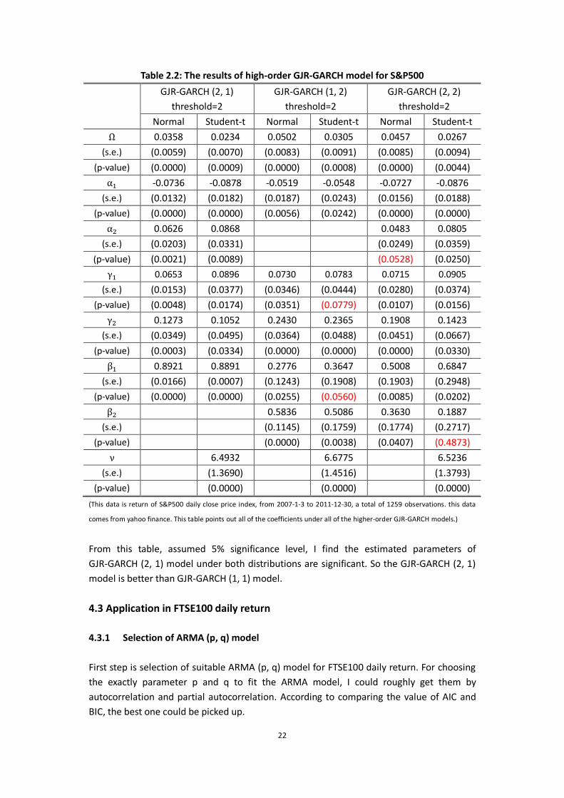
To sum up, both GARCH (1, 1) model and EGARCH (1, 1) model with normal distribution could explain the daily stock return better than GJR-GARCH (1, 1) model with two distributions. Because of the poor performance on GJR-GARCH (1, 1) model, I attempt to the high-order GJR-GARCH model, GJR-GARCH (1, 2) model, GJR-GARCH (2, 1) model and GJR-GARCH (2, 2) model with normal distribution and student-t distribution, and the results are shown in the Table 2.2.
22
Table 2.2: The results of high-order GJR-GARCH model for S&P500
GJR-GARCH (2, 1) threshold=2
GJR-GARCH (1, 2) threshold=2
GJR-GARCH (2, 2) threshold=2
Normal Student-t Normal Student-t Normal Student-t
Ω 0.0358 0.0234 0.0502 0.0305 0.0457 0.0267
(s.e.) (0.0059) (0.0070) (0.0083) (0.0091) (0.0085) (0.0094)
(p-value) (0.0000) (0.0009) (0.0000) (0.0008) (0.0000) (0.0044)
α -0.0736 -0.0878 -0.0519 -0.0548 -0.0727 -0.0876
(s.e.) (0.0132) (0.0182) (0.0187) (0.0243) (0.0156) (0.0188)
(p-value) (0.0000) (0.0000) (0.0056) (0.0242) (0.0000) (0.0000)
α 0.0626 0.0868 0.0483 0.0805
(s.e.) (0.0203) (0.0331) (0.0249) (0.0359)
(p-value) (0.0021) (0.0089) (0.0528) (0.0250)
γ 0.0653 0.0896 0.0730 0.0783 0.0715 0.0905
(s.e.) (0.0153) (0.0377) (0.0346) (0.0444) (0.0280) (0.0374)
(p-value) (0.0048) (0.0174) (0.0351) (0.0779) (0.0107) (0.0156)
γ 0.1273 0.1052 0.2430 0.2365 0.1908 0.1423
(s.e.) (0.0349) (0.0495) (0.0364) (0.0488) (0.0451) (0.0667)
(p-value) (0.0003) (0.0334) (0.0000) (0.0000) (0.0000) (0.0330)
β 0.8921 0.8891 0.2776 0.3647 0.5008 0.6847
(s.e.) (0.0166) (0.0007) (0.1243) (0.1908) (0.1903) (0.2948)
(p-value) (0.0000) (0.0000) (0.0255) (0.0560) (0.0085) (0.0202)
β 0.5836 0.5086 0.3630 0.1887
(s.e.) (0.1145) (0.1759) (0.1774) (0.2717)
(p-value) (0.0000) (0.0038) (0.0407) (0.4873)
ν 6.4932 6.6775 6.5236
(s.e.) (1.3690) (1.4516) (1.3793)
(p-value) (0.0000) (0.0000) (0.0000)
(This data is return of S&P500 daily close price index, from 2007-1-3 to 2011-12-30, a total of 1259 observations. this data
comes from yahoo finance. This table points out all of the coefficients under all of the higher-order GJR-GARCH models.)
From this table, assumed 5% significance level, I find the estimated parameters of GJR-GARCH (2, 1) model under both distributions are significant. So the GJR-GARCH (2, 1) model is better than GJR-GARCH (1, 1) model.
4.3 Application in FTSE100 daily return
4.3.1 Selection of ARMA (p, q) model
First step is selection of suitable ARMA (p, q) model for FTSE100 daily return. For choosing the exactly parameter p and q to fit the ARMA model, I could roughly get them by autocorrelation and partial autocorrelation. According to comparing the value of AIC and BIC, the best one could be picked up.
23
Many models have been tried, such as AR (1), MA (1), ARMA (1, 1) and so on. Finally, I choose p=1, q=1 because the ARMA (1, 1) has the smallest AIC and BIC of all the models. So I select the ARMA (1, 1) model finally. From the following function:
r = θ + θ e + θ r +e
The estimated parameters are θ = −0.01, θ = −0.7281 , θ = 0.6638
And then, calculate and take e = r − (θ + θ e + θ r ), after that estimate GARCH model on e . 4.3.2 Result of GARCH model and GARCH family model for FTSE100
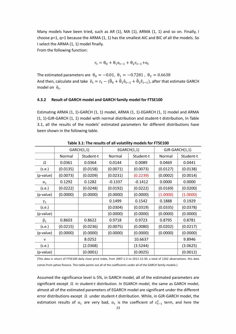
Estimating ARMA (1, 1)-GARCH (1, 1) model, ARMA (1, 1)-EGARCH (1, 1) model and ARMA (1, 1)-GJR-GARCH (1, 1) model with normal distribution and student-t distribution, In Table 3.1, all the results of the models’ estimated parameters for different distributions have been shown in the following table.
Table 3.1: The results of all volatility models for FTSE100
GARCH(1,1) EGARCH(1,1) GJR-GARCH(1,1)
Normal Student-t Normal Student-t Normal Student-t
Ω 0.0361 0.0364 0.0144 0.0089 0.0469 0.0441
(s.e.) (0.0135) (0.0158) (0.0071) (0.0073) (0.0127) (0.0138)
(p-value) (0.0073) (0.0209) (0.0231) (0.2239) (0.0002) (0.0014)
α 0.1292 0.1282 -0.1337 -0.1412 0.0000 0.0000
(s.e.) (0.0222) (0.0248) (0.0192) (0.0222) (0.0169) (0.0200)
(p-value) (0.0000) (0.0000) (0.0000) (0.0000) (1.0000) (1.0000)
γ 0.1499 0.1542 0.1888 0.1929
(s.e.) (0.0304) (0.0319) (0.0335) (0.0378)
(p-value) (0.0000) (0.0000) (0.0000) (0.0000)
β 0.8603 0.8622 0.9718 0.9723 0.8795 0.8781
(s.e.) (0.0215) (0.0236) (0.0075) (0.0080) (0.0202) (0.0217)
(p-value) (0.0000) (0.0000) (0.0000) (0.0000) (0.0000) (0.0000)
ν 8.0252 10.6637 9.8946
(s.e.) (2.0368) (3.5244) (3.0625)
(p-value) (0.0001) (0.0025) (0.0012)
(This data is return of FTSE100 daily close price index, from 2007-1-2 to 2011-12-30, a total of 1262 observations. this data
comes from yahoo finance. This table points out all of the coefficients under all of the GARCH family models.)
Assumed the significance level is 5%, in GARCH model, all of the estimated parameters are significant except Ω in student-t distribution. In EGARCH model, the same as GARCH model,
almost all of the estimated parameters of EGARCH model are significant under the different error distributions except Ω under student-t distribution. While, in GJR-GARCH model, the estimation results of α are very bad, α is the coefficient of ε term, and here the
24
p-value of α is very large, which represents the coefficient of ε is not significant and the
term of ε has no effect in interpretation of σ .
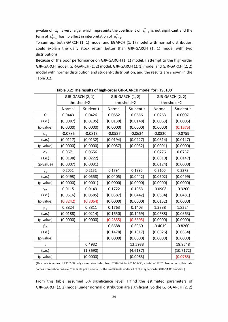
To sum up, both GARCH (1, 1) model and EGARCH (1, 1) model with normal distribution could explain the daily stock return better than GJR-GARCH (1, 1) model with two distributions. Because of the poor performance on GJR-GARCH (1, 1) model, I attempt to the high-order GJR-GARCH model, GJR-GARCH (1, 2) model, GJR-GARCH (2, 1) model and GJR-GARCH (2, 2) model with normal distribution and student-t distribution, and the results are shown in the Table 3.2.
Table 3.2: The results of high-order GJR-GARCH model for FTSE100
GJR-GARCH (2, 1) threshold=2
GJR-GARCH (1, 2) threshold=2
GJR-GARCH (2, 2) threshold=2
Normal Student-t Normal Student-t Normal Student-t
Ω 0.0443 0.0426 0.0652 0.0656 0.0263 0.0007
(s.e.) (0.0087) (0.0105) (0.0130) (0.0148) (0.0063) (0.0005)
(p-value) (0.0000) (0.0000) (0.0000) (0.0000) (0.0000) (0.1575)
α -0.0786 -0.0813 -0.0537 -0.0634 -0.0820 -0.0759
(s.e.) (0.0117) (0.0132) (0.0194) (0.0227) (0.0314) (0.0147)
(p-value) (0.0000) (0.0000) (0.0057) (0.0052) (0.0091) (0.0000)
α 0.0671 0.0656 0.0776 0.0757
(s.e.) (0.0198) (0.0222) (0.0310) (0.0147)
(p-value) (0.0007) (0.0031) (0.0124) (0.0000)
γ 0.2051 0.2131 0.1794 0.1895 0.2100 0.3272
(s.e.) (0.0493) (0.0558) (0.0405) (0.0442) (0.0502) (0.0499)
(p-value) (0.0000) (0.0001) (0.0000) (0.0000) (0.0000) (0.0000)
γ 0.0115 0.0143 0.1722 0.1953 -0.0908 -0.3200
(s.e.) (0.0516) (0.0585) (0.0387) (0.0442) (0.0634) (0.0481)
(p-value) (0.8242) (0.8064) (0.0000) (0.0000) (0.0152) (0.0000)
β 0.8824 0.8811 0.1763 0.1403 1.3338 1.8224
(s.e.) (0.0188) (0.0214) (0.1650) (0.1469) (0.0688) (0.0363)
(p-value) (0.0000) (0.0000) (0.2855) (0.3395) (0.0000) (0.0000)
β 0.6688 0.6960 -0.4019 -0.8260
(s.e.) (0.1478) (0.1317) (0.0626) (0.0354)
(p-value) (0.0000) (0.0000) (0.0000) (0.0000)
ν 6.4932 12.5933 18.8548
(s.e.) (1.3690) (4.6137) (10.7172)
(p-value) (0.0000) (0.0063) (0.0785)
(This data is return of FTSE100 daily close price index, from 2007-1-2 to 2011-12-30, a total of 1262 observations. this data
comes from yahoo finance. This table points out all of the coefficients under all of the higher-order GJR-GARCH models.)
From this table, assumed 5% significance level, I find the estimated parameters of GJR-GARCH (2, 2) model under normal distribution are significant. So the GJR-GARCH (2, 2)
25
model with normal distribution is better than GJR-GARCH (1, 1) model.
4.4 Application in NIKKEI daily return
4.4.1 Selection of ARMA (p, q) model
First step is selection of suitable ARMA (p, q) model for NIKKEI daily return. For choosing the exactly parameter p and q to fit the ARMA model, I could roughly get them by autocorrelation and partial autocorrelation. According to comparing the value of AIC and BIC, the best one could be picked up. Many models have been tried, such as AR (1), MA (1), ARMA (1, 1) and so on. Finally, I choose p=1, q=1 because the ARMA (1, 1) has the smallest AIC and BIC of all the models. So I select the ARMA (1, 1) model finally. From the following function:
r = θ + θ e + θ r + e
The estimated parameters are θ = −0.0589, θ = −0.7306, θ = 0.6812
And then, calculate and take e = r − (θ + θ e + θ r ), after that estimate GARCH model on e . 4.4.2 Result of GARCH model and GARCH family model for NIKKEI
Estimating ARMA (1, 1)-GARCH (1, 1) model, ARMA (1, 1)-EGARCH (1, 1) model and ARMA (1, 1)-GJR-GARCH (1, 1) model with normal distribution and student-t distribution, In Table 4.1, all the results of the models’ estimated parameters for different distributions have been shown in the following table.

26
Table 4.1: The results of all volatility models for NIKKEI
GARCH(1,1) EGARCH(1,1) GJR-GARCH(1,1)
Normal Student-t Normal Student-t Normal Student-t
Ω 0.0625 0.0500 0.0204 0.0168 0.0547 0.0504
(s.e.) (0.0239) (0.0238) (0.0081) (0.0083) (0.0193) (0.0197)
(p-value) (0.0090) (0.0352) (0.0122) (0.0416) (0.0045) (0.0104)
α 0.1339 0.1203 -0.1134 -0.1125 0.0178 0.0170
(s.e.) (0.0231) (0.0235) (0.0165) (0.0177) (0.0175) (0.0183)
(p-value) (0.0000) (0.0000) (0.0000) (0.0000) (0.3091) (0.3516)
γ 0.1515 0.1494 0.1493 0.1450
(s.e.) (0.0341) (0.0342) (0.0291) (0.0306)
(p-value) (0.0000) (0.0000) (0.0000) (0.0000)
β 0.8496 0.8674 0.9773 0.9790 0.8854 0.8894
(s.e.) (0.0239) (0.0245) (0.0069) (0.0069) (0.0209) (0.0209)
(p-value) (0.0000) (0.0000) (0.0000) (0.0000) (0.0000) (0.0000)
ν 13.5599 26.9464 26.9883
(s.e.) (6.0712) (20.6503) (23.9434)
(p-value) (0.0255) (0.1919) (0.2597)
(This data is return of NIKKEI daily close price index, from 2007-1-4 to 2011-12-30, a total of 1220 observations. this data
comes from yahoo finance. This table points out all of the coefficients under all of the GARCH family models.)
Assumed the significance level is 5%, in GARCH model, all of the estimated parameters are significant except Ω in student-t distribution. In EGARCH model, the same as GARCH model,
almost all of the estimated parameters of EGARCH model are significant under the different error distributions except Ω under student-t distribution. While, in GJR-GARCH model, the estimation results of α are very bad, α is the coefficient of ε term, and here the
p-value of α is very large, which represents the coefficient of ε is not significant and the
term of ε has no effect in interpretation of σ .
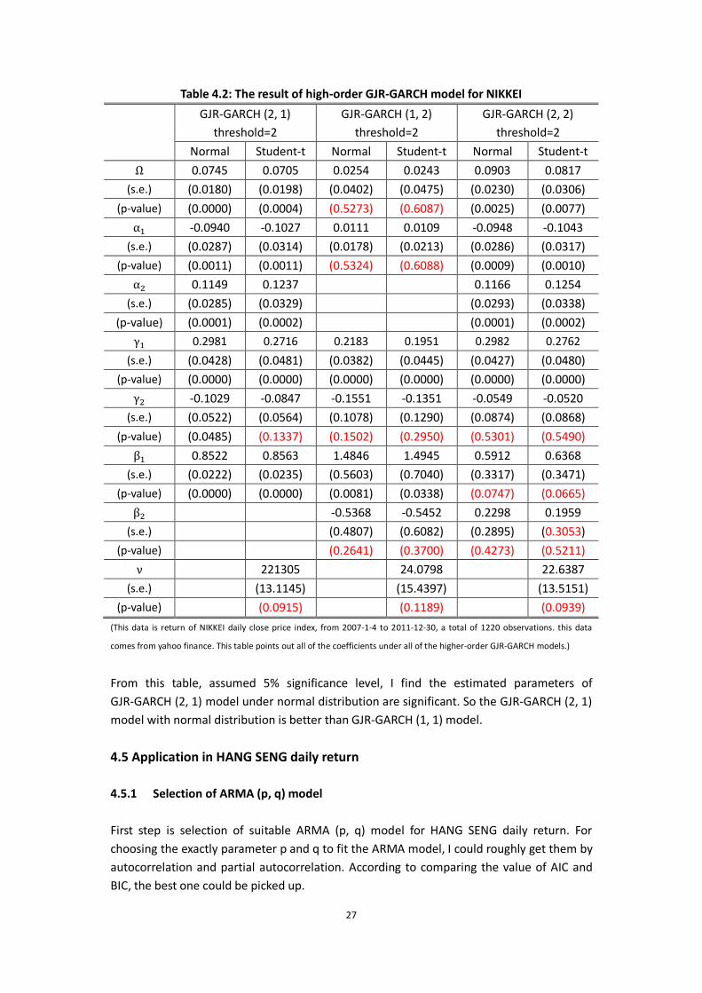
To sum up, both GARCH (1, 1) model and EGARCH (1, 1) model with normal distribution could explain the daily stock return better than GJR-GARCH (1, 1) model with two distributions. Because of the poor performance on GJR-GARCH (1, 1) model, I attempt to the high-order GJR-GARCH model, GJR-GARCH (1, 2) model, GJR-GARCH (2, 1) model and GJR-GARCH (2, 2) model with normal distribution and student-t distribution, and the results are shown in the Table 4.2.
27
Table 4.2: The result of high-order GJR-GARCH model for NIKKEI
GJR-GARCH (2, 1) threshold=2
GJR-GARCH (1, 2) threshold=2
GJR-GARCH (2, 2) threshold=2
Normal Student-t Normal Student-t Normal Student-t
Ω 0.0745 0.0705 0.0254 0.0243 0.0903 0.0817
(s.e.) (0.0180) (0.0198) (0.0402) (0.0475) (0.0230) (0.0306)
(p-value) (0.0000) (0.0004) (0.5273) (0.6087) (0.0025) (0.0077)
α -0.0940 -0.1027 0.0111 0.0109 -0.0948 -0.1043
(s.e.) (0.0287) (0.0314) (0.0178) (0.0213) (0.0286) (0.0317)
(p-value) (0.0011) (0.0011) (0.5324) (0.6088) (0.0009) (0.0010)
α 0.1149 0.1237 0.1166 0.1254
(s.e.) (0.0285) (0.0329) (0.0293) (0.0338)
(p-value) (0.0001) (0.0002) (0.0001) (0.0002)
γ 0.2981 0.2716 0.2183 0.1951 0.2982 0.2762
(s.e.) (0.0428) (0.0481) (0.0382) (0.0445) (0.0427) (0.0480)
(p-value) (0.0000) (0.0000) (0.0000) (0.0000) (0.0000) (0.0000)
γ -0.1029 -0.0847 -0.1551 -0.1351 -0.0549 -0.0520
(s.e.) (0.0522) (0.0564) (0.1078) (0.1290) (0.0874) (0.0868)
(p-value) (0.0485) (0.1337) (0.1502) (0.2950) (0.5301) (0.5490)
β 0.8522 0.8563 1.4846 1.4945 0.5912 0.6368
(s.e.) (0.0222) (0.0235) (0.5603) (0.7040) (0.3317) (0.3471)
(p-value) (0.0000) (0.0000) (0.0081) (0.0338) (0.0747) (0.0665)
β -0.5368 -0.5452 0.2298 0.1959
(s.e.) (0.4807) (0.6082) (0.2895) (0.3053)
(p-value) (0.2641) (0.3700) (0.4273) (0.5211)
ν 221305 24.0798 22.6387
(s.e.) (13.1145) (15.4397) (13.5151)
(p-value) (0.0915) (0.1189) (0.0939)
(This data is return of NIKKEI daily close price index, from 2007-1-4 to 2011-12-30, a total of 1220 observations. this data
comes from yahoo finance. This table points out all of the coefficients under all of the higher-order GJR-GARCH models.)
From this table, assumed 5% significance level, I find the estimated parameters of GJR-GARCH (2, 1) model under normal distribution are significant. So the GJR-GARCH (2, 1) model with normal distribution is better than GJR-GARCH (1, 1) model.
4.5 Application in HANG SENG daily return
4.5.1 Selection of ARMA (p, q) model
First step is selection of suitable ARMA (p, q) model for HANG SENG daily return. For choosing the exactly parameter p and q to fit the ARMA model, I could roughly get them by autocorrelation and partial autocorrelation. According to comparing the value of AIC and BIC, the best one could be picked up.
28
Many models have been tried, such as AR (1), MA (1), ARMA (1,1) and so on. Finally, I choose p=1, q=0 because the AR (1) has the smallest AIC and BIC of all the models. So I select the AR (1) model finally. From the following function:
r = θ + θ r + e
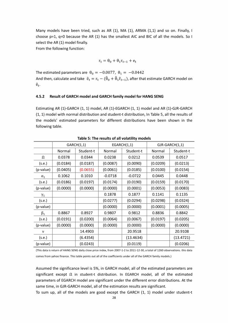
The estimated parameters are θ = −0.0077, θ = −0.0442 And then, calculate and take e = r − (θ + θ r ), after that estimate GARCH model on e . 4.5.2 Result of GARCH model and GARCH family model for HANG SENG
Estimating AR (1)-GARCH (1, 1) model, AR (1)-EGARCH (1, 1) model and AR (1)-GJR-GARCH (1, 1) model with normal distribution and student-t distribution, In Table 5, all the results of the models’ estimated parameters for different distributions have been shown in the following table.
Table 5: The results of all volatility models
GARCH(1,1) EGARCH(1,1) GJR-GARCH(1,1)
Normal Student-t Normal Student-t Normal Student-t
Ω 0.0378 0.0344 0.0238 0.0212 0.0539 0.0517
(s.e.) (0.0184) (0.0187) (0.0087) (0.0090) (0.0209) (0.0213)
(p-value) (0.0405) (0.0655) (0.0061) (0.0185) (0.0100) (0.0154)
α 0.1062 0.1010 -0.0718 -0.0722 0.0445 0.0448
(s.e.) (0.0186) (0.0197) (0.0174) (0.0190) (0.0159) (0.0170)
(p-value) (0.0000) (0.0000) (0.0000) (0.0001) (0.0053) (0.0083)
γ 0.1878 0.1877 0.1141 0.1135
(s.e.) (0.0277) (0.0294) (0.0298) (0.0324)
(p-value) (0.0000) (0.0000) (0.0001) (0.0005)
β 0.8867 0.8927 0.9807 0.9812 0.8836 0.8842
(s.e.) (0.0191) (0.0200) (0.0064) (0.0067) (0.0197) (0.0205)
(p-value) (0.0000) (0.0000) (0.0000) (0.0000) (0.0000) (0.0000)
ν 14.4903 20.9518 20.9108
(s.e.) (6.4354) (13.4634) (13.4721)
(p-value) (0.0243) (0.0119) (0.0206)
(This data is return of HANG SENG daily close price index, from 2007-1-2 to 2011-12-30, a total of 1260 observations. this data
comes from yahoo finance. This table points out all of the coefficients under all of the GARCH family models.)
Assumed the significance level is 5%, in GARCH model, all of the estimated parameters are significant except Ω in student-t distribution. In EGARCH model, all of the estimated parameters of EGARCH model are significant under the different error distributions. At the same time, in GJR-GARCH model, all of the estimation results are significant. To sum up, all of the models are good except the GARCH (1, 1) model under student-t
29
distribution.
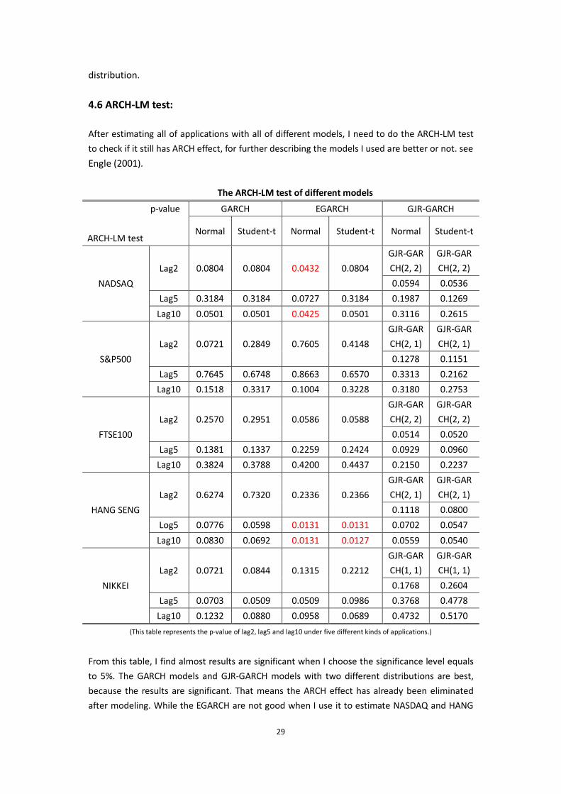
4.6 ARCH-LM test:
After estimating all of applications with all of different models, I need to do the ARCH-LM test
to check if it still has ARCH effect, for further describing the models I used are better or not. see
Engle (2001).
The ARCH-LM test of different models
p-value
ARCH-LM test
GARCH EGARCH GJR-GARCH
Normal Student-t Normal Student-t Normal Student-t
NADSAQ
Lag2 0.0804 0.0804 0.0432 0.0804
GJR-GAR
CH(2, 2)
GJR-GAR
CH(2, 2)
0.0594 0.0536
Lag5 0.3184 0.3184 0.0727 0.3184 0.1987 0.1269
Lag10 0.0501 0.0501 0.0425 0.0501 0.3116 0.2615
S&P500
Lag2 0.0721 0.2849 0.7605 0.4148
GJR-GAR
CH(2, 1)
GJR-GAR
CH(2, 1)
0.1278 0.1151
Lag5 0.7645 0.6748 0.8663 0.6570 0.3313 0.2162
Lag10 0.1518 0.3317 0.1004 0.3228 0.3180 0.2753
FTSE100
Lag2 0.2570 0.2951 0.0586 0.0588
GJR-GAR
CH(2, 2)
GJR-GAR
CH(2, 2)
0.0514 0.0520
Lag5 0.1381 0.1337 0.2259 0.2424 0.0929 0.0960
Lag10 0.3824 0.3788 0.4200 0.4437 0.2150 0.2237
HANG SENG
Lag2 0.6274 0.7320 0.2336 0.2366
GJR-GAR
CH(2, 1)
GJR-GAR
CH(2, 1)
0.1118 0.0800
Log5 0.0776 0.0598 0.0131 0.0131 0.0702 0.0547
Lag10 0.0830 0.0692 0.0131 0.0127 0.0559 0.0540
NIKKEI
Lag2 0.0721 0.0844 0.1315 0.2212
GJR-GAR
CH(1, 1)
GJR-GAR
CH(1, 1)
0.1768 0.2604
Lag5 0.0703 0.0509 0.0509 0.0986 0.3768 0.4778
Lag10 0.1232 0.0880 0.0958 0.0689 0.4732 0.5170
(This table represents the p-value of lag2, lag5 and lag10 under five different kinds of applications.)
From this table, I find almost results are significant when I choose the significance level equals
to 5%. The GARCH models and GJR-GARCH models with two different distributions are best,
because the results are significant. That means the ARCH effect has already been eliminated
after modeling. While the EGARCH are not good when I use it to estimate NASDAQ and HANG

30
SENG daily stock price.
4.7 Out-of-sample Forecasts
In this paper, I choose to calculate the root mean square error (RMSE) with out-of-sample to
acquire the best model to forecast the financial volatility. Even though I also could determine a
model is good or not by comparing the AIC, BIC, log likelihood and so on, while these kind of
ways are not always give us the exactly decision. And next, I will explain how to operate this
procedure to acquire RMSE from the out-of-sample. See Forsberg and Bollerslev (2002). I use
the NASDAQ daily return as an example to explain it in details. The NASDAQ daily return
includes 1259 observations, five years, and I reserve the last year data as out-of-sample,
including 252 observations. For forecasting I use in-sample data including the first 1007
observations as the window, so the length of window is 1007 which is fixed. Firstly, I pick up the
observations from 1 to 1007 into this fixed window to estimate parameters with GARCH and
extension GARCH model. Then I can get the first forecasting value of the conditional variance.
This process is called as one-step-ahead forecast. Secondly, I repeat the first step except
change the observations from 2 to 1008 in the fixed window, and get the second forecasting
value of the conditional variance. Next, I repeat the first step except change the observations
from 3 to 1009 in the fixed window, and get the third forecasting value of the conditional
variance. This step will be repeated one by one, total 252 times. Then getting 252 forecasting
value of the conditional variance, so such a process is named as multi-step-ahead forecast.
Then I use the 252 forecasting value of the conditional variance to calculate the RMSE by the
formula (7). For other four applications, the detailed descriptions about how to calculate the
RMSE could be checked from the Appendix B. Check them from Appendix B if you want to get
more details.
At last, by comparing to the different RMSEs with all the GARCH and extension GARCH models
in different returns data, I could choose the smallest one and decide which model is the best
one. And the RMSE of different models for all of applications are shown as the following Table
6.

31
Table 6:The result of RMSE about five different stock’s daily return
RMSE
NASDAQ GARCH (1,1)-Normal 5.4266
GARCH (1,1)-student-t 5.4559
EGARCH (1,1)-Normal 6.6210
EGARCH (1,1)-student-t 6.2907
GJR-GARCH (2,2)-Normal 5.3727
GJR-GARCH (2,2)-student-t 5.3980
RMSE
S&P500 GARCH (1,1)-Normal 4.9267
GARCH (1,1)-student-t 4.9545
EGARCH (1,1)-Normal 6.5879
EGARCH (1,1)-student-t 7.2929
GJR-GARCH (2,1)-Normal 4.9135
GJR-GARCH (2,1)-student-t 4.9410
RMSE
FTSE100 GARCH (1,1)-Normal 3.3983
GARCH (1,1)-student-t 3.3975
EGARCH (1,1)-Normal 5.9724
EGARCH (1,1)-student-t 4.1848
GJR-GARCH (2,2)-Normal 3.3695
GJR-GARCH (2,2)-student-t 3.3776
RMSE
HANG SENG GARCH (1,1)-Normal 5.2545
GARCH (1,1)-student-t 5.2585
EGARCH (1,1)-Normal 6.1322
EGARCH (1,1)-student-t 5.6013
GJR-GARCH (2,1)-Normal 5.3045
GJR-GARCH (2,1)-student-t 5.3063
RMSE
NIKKEI GARCH (1,1)-Normal 8.6513
GARCH (1,1)-student-t 8.7123
EGARCH (1,1)-Normal 9.4638
EGARCH (1,1)-student-t 9.3891
GJR-GARCH (1,1)-Normal 8.5685
GJR-GARCH (1,1)-student-t 8.5938
Here, I need to pick up the smaller value for each kind of stock daily return from this table, for all of the data, the RMSEs of higher-order GJR-GARCH model with normal distribution are smallest for NASDAQ, S&P500, FTSE100 and NIKKEI, and the GARCH model with normal distribution is smallest for HANG SENG. And the RMSE of the entire EGARCH models are larger than other models, so the EGARCH models are worst.

32
5. Conclusion
Based on five different financial volatility data, I use the different model to estimate separately and choose the normal distribution and the student-t distribution as the error term distribution. By comparing the result of the RMSE, I could obviously get which model is the most suitable to forecast the conditional variance of financial data in NASDAQ, Standard & Poor 500, FTSE100, HANG SENG and NIKKEI stock index. For different applications, the best model is different. The RMSE’s values about GJR-GARCH model are smallest compared with other models, so GJR-GARCH model is a good model for predicting. For NASDAQ daily return, GJR-GARCH (2, 2) model with normal distributions could explain better than other models, for S&P500 daily return, GJR-GARCH (2, 1) model with normal distributions could explain better than other models, for FTSE100 daily return, GJR-GARCH (2, 2) model with normal distribution could explain better than other models, for NIKKEI daily return, GJR-GARCH (2,1) model with normal distribution could explain better than other models, for HANG SENG daily return, GARCH model with normal distribution could explain better than other models. From these conclusion mentioned above, I find some shortcomings and deficiencies about the models I used. So the drawbacks of models maybe lead to the poor estimation for data, which cannot predict the conditional variance exactly. So from this perspective and aim, maybe I could add some extra extension models in my paper, and consider about more factors which explained data better, and then put the factors in the model to do further study and get the better prediction. In addition to internal factors, it still has some external factors affect the accuracy of the model, such as: economic factors, political environment, policy changes and so on. Economic factor includes some cyclical changes in economic, for instance, global financial crisis and prosperity will affect the stock price directly. At the same time, some new government fiscal and monetary policies also increase or decrease the stock market. So I could add some steps to check if stock price exist structure break. If it exist break points, and separate the series into subseries according to the location of the break-points, and fit different GARCH models to the subseries. After eliminating the structure break, maybe the result could be modified and expressed better. Thus the main statistical problem is how to find the number of break-points and their location because they cannot be observed in advance. Chu (1995) has developed tests for this purpose.

33
6. Reference
6.1 article resource
Alexander, C. and Lazar, E., 2006, Normal mixture GARCH (1, 1): application to exchange rate modeling. Journal of Applied Econometrics Economic Review, 39: 885–905.
Alexander, C. and Lazar, E., 2004, The equity index skew, market crashes and asymmetric normal mixture GARCH. ISMA Center Discussion Papers in Finance, 14.
Andersen, T. G. and Bollerslev, T., 1998, Answering the skeptics: Yes, standard volatility models provide accurate forecasts. International Economic Review, 39: 885-905.
Baillie, R. T. and Bollerslev, T., 1989, Common stochastic trends in a system of exchange rates. Journal of Monetary Economics, 44: 167-181.
Baillie, R. T., Bollerslev, T. and Mikkelsen, H. O., 1996, Fractionally integrated generalized autoregressive conditional heteroskedasticity. Journal of Econometrics, 74: 3-30.
Bollerslev, T., 1986, Generalized autoregressive conditional heteroskedasticity. Journal of Econometrics, 31: 307-327.
Bollerslev, T., 1987, A conditionally heteroskedastic time series model for speculative prices and rates of return. Review of Economics and Statistics, 147-165.
Bollerslev, T. and Mikkelsen, H.O., 1996, Modeling and pricing long memory in stock market volatility. Journal of Econometrics, Elsevier, vol. 73(1): 151-184.
Bollerslev, T., Chou, R. Y. and Kroner, K. F., 1992, ARCH modeling in finance: A review of the theory and empirical evidence. Journal of Econometrics, 52: 5-59.
Brailsford, T. and Faff, R., 1996, An evaluation of volatility forecasting techniques. Journal of Banking and Finance, 20: 119-138.
Chu, C. S. J., 1995, Detecting parameter shift in GARCH models. Econometric Reviews, 14:
241-266.
Enocksson, D. and Skoog, J., 2012, Evaluating VaR with the ARCH/GARCH family. Bachelor thesis,
Fall 201102, 3-4. Available from: http://www.essays.se/essay/6c2c73ed2d/
Engle, R. F., 1982, Autoregressive conditional heteroscedasticity with estimates of the variance of United Kingdom inflation. Econometrica, 50: 987–1007.
Engle, R. F. and Bollerslev, T., 1986, Modeling the persistence of conditional variances, Econometric Reviews. Taylor and Francis Journals, vol. 5(1): 1-50.
Engle, R. F., 2001, GARCH 101: The use of ARCH/GARCH models in applied econometrics. Journal of Economic Perspectives, vol. 15(4): 157–168.
Engle, R. F., 2002, New frontiers For ARCH models. Journal of Applied Econometrics, 17: 425–446.
French, K. R., Schwert, G. W. and Stambaugh, R. F., 1987, Expected stock returns and volatility. Journal of Financial Economics, 19: 3–30.
Forsberg, L. and Ghysels, E., 2007, Why do absolute returns predict volatility so well? Journal of Financial Econometrics, 5: 50–67.
Forsberg, L. and Bollerslev, T., 2002, Bridging the gap between the distribution of realized (ECU) volatility and ARCH modeling (of the EURO): the GARCH-NIG model. Journal of Applied Econometrics, 17: 535–548.
34
Franses, P. H. and Mcaleer, M., 2002, Financial volatility: An Introduction. Journal of Applied Econometrics, 17: 419–424.
Glosten,L., Jangannathan, R. and Runkle, D., 1993, On the relation between excepted value and the volatility of the nominal excess return of stocks. Journal of Finance, 48: 1779-1801.
He, C. and Teräsvirta, T., 1999, Properties of the autocorrelation function of squared observations for second order GARCH processes under two sets of parameter constraints. Journal of Time Series Analysis, 20: 23-30.
Nelson, D., 1991, Conditional heteroskedasticity in asset returns: a new approach. Econometrics, 59: 349–370.
Nelson, D. B. and Cao, C. Q., 1992, Inequality constraints in the univariate GARCH model. Journal of Business and Economic Statistics, 10: 229-235.
Patrick, D., Stewart, M. and Chris. S., 2006, Stock returns, implied volatility innovations, and the asymmetric volatility phenomenon. Journal of Financial and Quantitative Analysis, 41: 381-406.
Rabemananjara, R. and Zakoian, J. M., 1993, Threshold Arch Models and Asymmetries in Volatility. Journal of Applied Econometrics, 8(1): 31–49.
Teräsvirta, T., 2006, An introduction to univariate GARCH models, SSE/EFI. Working Papers in Economics and Finance, No. 646.
Wang, K. L., Fawson, C., Barrett, C. B. and Mcdonald, J. B., 2001, A flexible parametric GARCH model with an application to exchange rates. Journal of Applied Econometrics, 16: 521–536.
6.2 websites resource Wikipedia: Root-mean-square deviation,
http://en.wikipedia.org/wiki/Root-mean-square_deviation
Yahoo finance: S&P500 historical prices, http://finance.yahoo.com/q/hp?s=%5EGSPC+Historical+Prices
Yahoo finance: NASDAQ historical prices, http://finance.yahoo.com/q/hp?s=%5EIXIC+Historical+Prices
Yahoo finance: FTSE100 historical prices, http://finance.yahoo.com/q/hp?s=%5EFTSE+Historical+Prices Yahoo finance: HANG SENG historical prices,
http://finance.yahoo.com/q/hp?s=%5EHSI+Historical+Prices Yahoo finance: NIKKEI historical prices,
http://finance.yahoo.com/q/hp?s=%5EN225+Historical+Prices

35
7. Appendix
7.1 Appendix A:ACF and PACF about return value
0 15 30
0.0
0.2
0.4
0.6
0.8
1.0
Lag
auto
corre
latio
n
NASDAQ.ACF
0 15 30
-0.1
0-0
.05
0.00
0.05
Lag
part.
auto
corre
latio
n
NASDAQ.PACF
0 15 30
0.0
0.2
0.4
0.6
0.8
1.0
Lagau
toco
rrela
tion
S&P.ACF
0 15 30
-0.1
0-0
.05
0.00
0.05
Lag
part.
auto
corre
latio
n
S&P.PACF
0 15 30
0.0
0.2
0.4
0.6
0.8
1.0
Lag
auto
corre
latio
n
FTSE100.ACF
0 15 30
-0.0
50.
000.
050.
10
Lag
part.
auto
corre
latio
n
FTSE100.PACF
0 15 30
0.0
0.2
0.4
0.6
0.8
1.0
Lag
auto
corre
latio
n
NIKKEI.ACF
0 15 30
-0.1
0-0
.05
0.00
0.05
Lag
part.
auto
corre
latio
n
NIKKEI.PACF
0 15 30
0.0
0.2
0.4
0.6
0.8
1.0
Lag
auto
corre
latio
n
HANG SENG.ACF
0 15 30
-0.0
50.
000.
05
Lag
part.
auto
corre
latio
n
HANG SENG.PACF
36
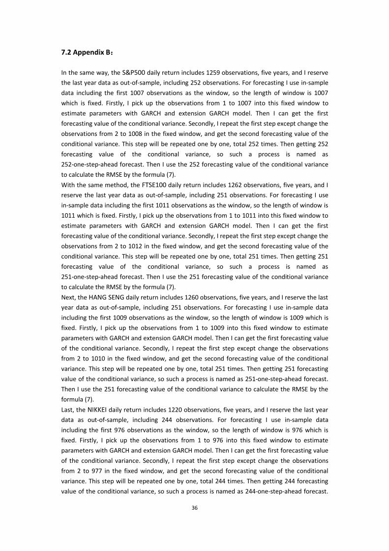
7.2 Appendix B:
In the same way, the S&P500 daily return includes 1259 observations, five years, and I reserve
the last year data as out-of-sample, including 252 observations. For forecasting I use in-sample
data including the first 1007 observations as the window, so the length of window is 1007
which is fixed. Firstly, I pick up the observations from 1 to 1007 into this fixed window to
estimate parameters with GARCH and extension GARCH model. Then I can get the first
forecasting value of the conditional variance. Secondly, I repeat the first step except change the
observations from 2 to 1008 in the fixed window, and get the second forecasting value of the
conditional variance. This step will be repeated one by one, total 252 times. Then getting 252
forecasting value of the conditional variance, so such a process is named as
252-one-step-ahead forecast. Then I use the 252 forecasting value of the conditional variance
to calculate the RMSE by the formula (7).
With the same method, the FTSE100 daily return includes 1262 observations, five years, and I
reserve the last year data as out-of-sample, including 251 observations. For forecasting I use
in-sample data including the first 1011 observations as the window, so the length of window is
1011 which is fixed. Firstly, I pick up the observations from 1 to 1011 into this fixed window to
estimate parameters with GARCH and extension GARCH model. Then I can get the first
forecasting value of the conditional variance. Secondly, I repeat the first step except change the
observations from 2 to 1012 in the fixed window, and get the second forecasting value of the
conditional variance. This step will be repeated one by one, total 251 times. Then getting 251
forecasting value of the conditional variance, so such a process is named as
251-one-step-ahead forecast. Then I use the 251 forecasting value of the conditional variance
to calculate the RMSE by the formula (7).
Next, the HANG SENG daily return includes 1260 observations, five years, and I reserve the last
year data as out-of-sample, including 251 observations. For forecasting I use in-sample data
including the first 1009 observations as the window, so the length of window is 1009 which is
fixed. Firstly, I pick up the observations from 1 to 1009 into this fixed window to estimate
parameters with GARCH and extension GARCH model. Then I can get the first forecasting value
of the conditional variance. Secondly, I repeat the first step except change the observations
from 2 to 1010 in the fixed window, and get the second forecasting value of the conditional
variance. This step will be repeated one by one, total 251 times. Then getting 251 forecasting
value of the conditional variance, so such a process is named as 251-one-step-ahead forecast.
Then I use the 251 forecasting value of the conditional variance to calculate the RMSE by the
formula (7).
Last, the NIKKEI daily return includes 1220 observations, five years, and I reserve the last year
data as out-of-sample, including 244 observations. For forecasting I use in-sample data
including the first 976 observations as the window, so the length of window is 976 which is
fixed. Firstly, I pick up the observations from 1 to 976 into this fixed window to estimate
parameters with GARCH and extension GARCH model. Then I can get the first forecasting value
of the conditional variance. Secondly, I repeat the first step except change the observations
from 2 to 977 in the fixed window, and get the second forecasting value of the conditional
variance. This step will be repeated one by one, total 244 times. Then getting 244 forecasting
value of the conditional variance, so such a process is named as 244-one-step-ahead forecast.

37
Then I use the 244 forecasting value of the conditional variance to calculate the RMSE by the
formula (7).