Embed Size (px)
Citation preview

Modeling and Measuring Volatility in the Black-Scholes Economy:
A Bayesian Approach
Giuseppe Russo, A.S.A. Graduate Student
Department of Industrial Engineering and Operations Research University of California, Berkeley
Berkeley, CA 94720 U.S.A.
Fax: (510) 642-1403
Summary
The Black-Scholes economy model with constant drift and volatility is used as a first attempt
to statistically analyze stock volatility. A posterior distribution of market volatility given
past stock prices is derived using a Bayesian approach. A market analyst would incorporate
his/her personal knowledge through the specification of a prior distribution. The natural
conjugate prior is a Normal-Generalized Inverse Gaussian distribution with five
hyperparameters. The posterior mean and mode take a credibility form that is a weighted
average of three different volatility measurements. Specifying these weights along with
other easily calculated market measurements allows the analyst to indirectly obtain the prior
distribution. European options are priced by calculating the expected value of the Black-
Scholes formula using the posterior distribution of stock volatility. A set of historical S&P 500
data is numerically analyzed to illustrate results.
* This paper will be part of a Ph.D. thesis by the author at University of California, Berkeley.
609

Mod&le et mesure de la volatilit6 dans 1’6conomie Black-Scholes : Une m&hode bayesienne’
Giuseppe Russo, A.S.A. Etudiant de troisieme cycle
Departement de recherche industrielle et operationnelle Universite de Californie, Berkeley
Berkeley, CA 94720 Etats-Unis
Fax : (510) 642-1403
R&urn6
Le modele Bconomique Black-Scholes de volatilite et de derive constante est
utilise pour tenter pour la premiere fois d’analyser statistiquement la volatilite
des actions. Une distribution posterieure de la volatilite du marche tenant
compte du prix anterieur des actions est derivee par methode bayesienne. Un
analyste du marche incorporerait ses connaissances personnelles en specifiant
la distribution anterieure. Le conjugat anterieur est une distribution gaussienne
inverse normale-generalisee comportant cinq hyperparametres. Le mode et la
moyenne posterieure se presentent sous forme previsible qui est la moyenne
pond&he de trois mesures de volatilite differentes. La specification de ces
ponderances et d’autres mesures du marche aisement calculees permet a
I’analyste d’obtenir indirectement la distribution anterieure. Le prix des options
europeennes est Btabli en calculant la valeur anticipee de la formule Black-
Scholes Zr I’aide de la distribution posterieure de la volatilite des actions. Un
ensemble de donnees S&P 500 historiques est analyst! numeriquement pour
illustrer les resultats.
l
Le present expose fera partie d’une these de doctorat pieparee par
I’auteur B I’Universite de Californie, Berkeley.
610

MODELING AND MEASURING VOLATILITY 611
1. Introduction
Stock options have become important instruments in portfolio management and other
fields of finance. The pricing of these and many other derivative securities requires the use of
formulae that rely heavily on measurements of stock volatility. For example, the well-known
Black&holes pricing formula for European options does not require the use of a stock’s mean
return but does depend on stock volatility measurements in its calculations. Dynamic portfolio
insurance strategies require variances and covariances of many assets to construct hedged
portfolios. The magnitude of underlying stock volatility directly contributes to the cost of
constructing and maintaining these hedged portfolios.
Empirical evidence by Black (1976) shows that stock market volatility is negatively
correlated with market performance. In periods of market down turns, increases in market
volatility are observed. When stock prices are rising, the volatility is significantly lower.
The model proposed in this paper could reflect this observed behaviour but for simplifying
reasons, and the lack of information available concerning this phenomenon (for various
theories, see Malkie1(1979), Modigliani and Cohn (1979), Fama (1981), Pindyck (1984) and
Chou(1988)), it will not be incorporated into the analysis.
Hence, volatility is not a simple parameter to estimate. Many innovative techniques
have been introduced and empirically tested including Autoregressive Conditional
Heteroskedasticity models (ARCH) and continuous stochastic volatility models. Bollerslev,
Chou and Kroner (1992) present a survey of ARCH model in finance. This review of the
literature includes both theoretical and empirical results.
Hull and White (1987) analyze the pricing of options under stochastic volatility.
Wiggins (1987) also solves the call option valuation problem assuming a continuous stochastic
process for return volatility and uses this model to derive statistical estimators. Mean

612 4TH AFIR INTERNATIONAL COLLOQUIUM
reversion models have been considered and used by Cox, fngersol and Ross (1985), Hull and
White (1988) and Randolph (1991).
In this paper, the problem of measuring volatility in the Black&holes economy using
a Bayesian statistical approach is considered. This first attempt assumes that the drift and
volatility components of the underlying stock price are constant over time. This assumption
will be relaxed in future papers. Observed fluctuations in stock prices will be used to derive a
posterior distribution for the underlying volatility. The model used to obtain the likelihood
for the observed data is the same model used to derive the Black&holes option formula.
The posterior distribution of the underlying volatility performs two useful purposes.
First, it can be integrated with the Black-Scholes formula to obtain option prices of the
underlying stock without requiring point estimates of the volatility. Unlike classical
statistical approaches, this Bayesian analysis relies on a prior distribution so that the market
analyst can incorporate his/her own beliefs in pricing option instruments. Second, it is
extremely difficult for traditional methods to provide accurate measurements of volatility
uncertainty. Variances of point estimators could be calculated but they do not completely
reveal the uncertainty of information. Furthermore, it is extremely difficult to incorporate
variances of volatility estimates into option pricing formulae. The posterior distribution
graphically illustrates increases (or decreases) in uncertainty of the underlying stock volatility
through increases (or decreases) in the dispersion of the distribution. This is illustrated
through numerical analysis of historical S&P 500 observations.
The prior distribution can be thought of as the information or knowledge the
professional market analyst believes about the underlying stock volatility. Although the
functional form of the prior distribution proposed may seem complicated and too abstract for a
practical user to specify (the prior distribution requires the specification of five parameters), it

MODELING AND MEASURING VOLATILITY 613
will be shown that the prior’s parameters exhibit intuitive and natural interpretations that
will be of assistance in specify their values.
Assume that the information structure in this economy is determined by a standard
Brownian motion W(s) and the filtration process
F,=o{W(s); Olslt}. (1)
Associated with this filtration process are two securities. The first is a riskless asset whose
value at time t is represented by
B(t) = B(O)@ (2)
where r is a fixed constant representing the “force of interest”. The second security is the stock
and it value at time t is represented by
(3)
where p is the drift constant and cr2 is the underlying volatility.
This model was used by Black and Scholes (1973), Merton (1973), Cox and Huang (1986)
and many others to develop the theory of option pricing. A “no arbitrage” argument either by
the use of martingales or other discrete means in conjunction with the above model can be used to
derive the Black-Scholes formula for pricing call options as
C(tp(t),K,r,T,oZ)=S(t)N 2 ! 2 + f0JT-t 1 ( - Ke-‘(T-‘h 2 - +TT 1 t4) where
Z= ln(S(t)/K)+r(T-t)
a&e ’ (5)

614 4TH AFIR INTERNATIONAL COLLOQUIUM
K is strike price, T is maturity date and N(x) is the cumulative standard Normal D&ribution.
All variables in this formula are known quantities (or may be estimated fairly accurately)
except the volatility o* of the underlying stock.
2. Likelihood Equation and Observed Data
The security is observed over a specified period of time. Sample values of the stock
price are observed and recorded along with the exact time the observations are taken, Let
D = {(ti, S(ti)); i = 1, . . .,n represent the set of data that is collected. Without loss of }
generality, assume t, I 0 and S( to) = 1. For this general model, observations need not be made at
equal time intervals. From equation (3) and the well-known fact that the standard Brownian
Motion has stationary and independent increments, the difference in logarithmic stock prices
lnS(ti) - lnS(fiel), given drift p and volatility cr*, are independent normally distributed with
mean (p - 0.5u2)(ti - tiwl) an variance 02(ti - t,-l). Therefore, the likelihood of the observed d
data is
(In[S(ti)lS(ti-~)]-(~-0.5U2)(ti - ti-1)) U2(ti - ti-1) (6)
For notation convenience, let
Then, the likelihood can be reduced to
(7)
From this equation, it is easily seen that all the data can be reduced to four sufficient statistics,
namely n, t, , R, and R,.
MODELING AND MEASURING VOLATILITY 615
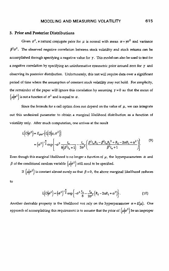
3. Prior and Posterior Distributions
Given CT’, a natural conjugate prior for /L is normal with mean a+ *p2 and variance
p2u2. The observed negative correlation between stock volatility and stock returns can be
accomplished through specifying a negative value for y . This model can also be used to test for
a negative correlation by specifying an uninformative symmetric prior around zero for y and
observing its posterior distribution. Unfortunately, this test will require data over a significant
period of time where the assumption of constant stock volatility may not hold. For simplicity,
the remainder of the paper will ignore this correlation by assuming y = 0 so that the mean of
(I 1 p u2 is not a function of cr2 and is equal to a.
Since the formula for a call option does not depend on the value of /J, we can integrate
out this undesired parameter to obtain a marginal likelihood distribution as a function of
volatility only. After much computation, one arrives at the result
p2t,R2-~2t,R,2+RP-2aR1+a2
)I
(9)
p2t, + 1
Even though this marginal likelihood is no longer a function of p, the hyperparameters 01 and
P of the conditional random variable (~16~) still need to be specified.
If (111 rr ‘1 is constant almost surely so that p = 0, the above marginal likelihood reduces
to
Another desirable property is the likelihood not rely on the hyperparameter a=E(p). One
approach of accomplishing this requirement is to assume that the prior of (+‘) be an improper

616 4TH AFIR INTERNATIONAL COLLOQUIUM
uniform prior. This is equivalent to assuming beta large. As fl+ 0, the limiting posterior
distribution is
(11)
Returning to the general form of the likelihood in equation (9), the natural conjugate
prior distribution for cr2 takes the form
p(02) = (02)+ exp{-o’$ --&a} (13)
where A,, Ba and C, are chosen so that ~(a’) is a proper distribution. Using Bayes Theorem,
the posterior distribution for o2 given the observed data D is
p(o’ID) = E,,,+(Dl~fio~))~(o~)
= (cr’)‘exp{-0’8, -SC”)
where
A,, =&+n,
B, =B, + ” f3(P2f, + 1)
and
(14)
(15)
The probability density function
f(xlA, B, C) = x-4 exp (16)
is the General Inverse Gaussian Distribution. With the integrating constant included, the
probability density function is

MODELING AND MEASURING VOLATILITY 617
f(*lA, B, C) = (& x-8 exp (17)
where K,,(x) is the Modified Bessel Function of the Second Kind. For a more thorough
discussion of Bessel functions, refer to Abramowitz and Stegun (1965), Press et al. (1988) or
Relton (1965). K,,(x) has a singularity at x=0. Thus, (17) is only valid for B,C > 0. Jorgensen
(1982) gives a detailed statistical analysis of this distribution.
If C = 0 and A’= -4 + l> 0 then the density function takes the limiting Gamma
Distribution form
If B = 0 and A’ = 9 - 1> 0 then the limiting distribution is the Inverse Gamma distribution.
With the change of variables A = 2(v+l), B = + and C = 1, the distribution is u
transformed into
(19)
Note that this transformation is not a complete mapping between the (A,B,C) space and the
(u, L, p) space. There are no corresponding points in the (n, 11, p) space that corresponds to the
values where BC = 0 but B or C > 0. This second parameterization has two advantages. If
v=O.5 then one obtains the standard Inverse Gaussian Distribution
(20)
Also, if p = 1 then the above distribution reduces to the standard Wald Distribution (for more
information regarding these distributions, see Johnson and Kotz (1970).) Second, the nth
moments of the random variable X takes the convenient form
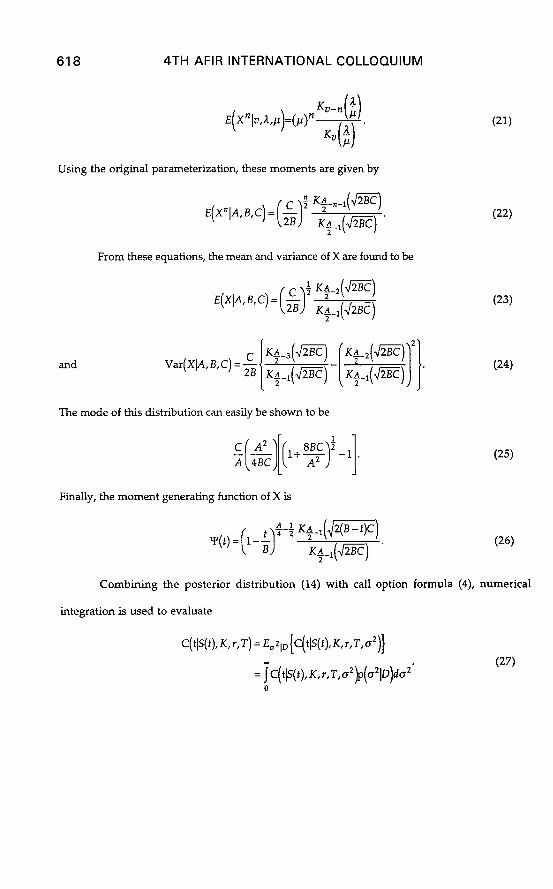
618 4TH AFIR INTERNATIONAL COLLOQUIUM
Using the original parameterization, these moments are given by
and
From these equations, the mean and variance of X are found to be
(22)
(23)
(24)
(25)
The mode of this distribution can easily be shown to be
Finally, the moment generating function of X is
Combining the posterior distribution (14) with call option formula (4), numerical
integration is used to evaluate
C(tlS(r),K,r,T)=E,21,[C(tlS(t),K,r,T,~2)]
= qjc(tlS(t),K,r,T,a2~(~‘1D)do2’ 0
(27)

MODELING AND MEASURING VOLATILITY 619
By differentiating the Black-Scholes formula with respect to 02, it can easily be demonstrated
that C(tlS(t), K, r, T,cr’) is a convex function for small values of a2 and concave for large values.
That is, for
C(o’) is a concave function. Hence, if P(02 > ZID) is close to one then by Jensen’s Inequality,
When uncertainty in the market is small so that P(02 > ZID) is small,
(29)
(30)
The conditional probability P(a2 > IID) . 1s c 1 ose to zero under one of the following two
conditions: (i) stock volatility is small, or (ii) the value of 1 is large. If conditions (i) is
satisfied then during periods of low stock volatility, the Black-Scholes formula tends to
undervalue European call options. Similarly, conditions (ii) says that the Black-Scholes
formula tends to undervalue European call options for deep-out-of-the-money or deep-in-the-
money options. On the other hand, the Black-Scholes formula tends to overvalue European call
options when market volatility is high or when the call option is at-the-money. These results
extend findings obtained by Hull and White (1987) derived with stochastic volatility and
agree with results obtained by Merton (1976) in conjunction with mixed jump-diffusion processes.
4. Parameter Interpretation of Prior Distributions
This section of the paper will discuss an approach that may be used to specify a prior
distribution on o2 based on subjective beliefs of the stock market analyst. Recall from Section 3,
the prior is parameterized by five variables that require specification. In particular, they are

4TH AFIR INTERNATIONAL COLLOQUIUM
A,,, B, , C,, CY and p. It was also shown in Section 2 that the stock data can be summarized
into the four summary statistics n, t,, R, and R,. From equation (15), the updating of the prior
by the observed stock prices is given by
A,, =A,+n
Bn = B. + .q*; +q
and
We will begin the analysis with two special cases for the prior whose interpretation
will help us in the general case. First, assume that observations are taken at equal time
intervals of length A so that t, = An. It can further be assumed that A=1 with the
understanding that all market statistics referred to in the remainder of the paper are measured
in the same unit of time as the observed stock prices. With this assumption, it is trivial to
show that
Also, the mode of the posterior distribution is
(32)
‘. (33)
Since (1+ x$ - 1 - x/2 for small x and lim BC a = 0, the above mode is approximately equal to
?I+- A,2
$ for large values of n. n
The first special case we will look at is the improper uniform prior for ($?). Recall
that this is equivalent to letting p + m. In this case, the mode of the posterior distribution can
be written in the credibility form as

MODELING AND MEASURING VOLATILITY 621
lf Boco co 2 IS small then - is a good approximation of the mode of the prior distribution while A, Ao
R, -RI is the estimate of stochastic volatility using sample data only. The posterior mode is a
weighted average of these two values, the size of the weights depending on the value of the
prior specified parameter A, and the number of observations n.
Next, we will look at the other extreme of this prior distribution. Namely, when the
prior value of (PI o ‘] 1s specified to be equal to a known constant 01 with no volatility. That is,
p = 0. In this case, the mode of the posterior distribution takes the credibility form
~=(~)(~)+(~)(R,-2nR,+a’). (35)
Again, G is the mode of the prior distribution but this time, since the drift parameter p is Ao
known to be equal to 01 with certainty, the estimate of stock volatility using observed returns is
given by the expression
Hence, the posterior mode is again the weighted average of the prior mode and the sample
estimate of stock volatility using the observed data only with the same weights as before.
The two previous special cases can now be of assistance in analyzing the general case
more easily. For any specified fixed value of fl, the posterior mode can be written in the
credibility form
622 4TH AFIR INTERNATIONAL COLLOQUIUM
In light of the above special cases, this equation tells us that the posterior mode is the
weighted sum of three volatility measures. The first measure is the mode of the prior
distribution. This measure is given the largest weight when little data is available. The next
measure is the volatility measure with the hyperparameter a playing the role of the mean
drift p. The final measure of volatility in this formula is the sample estimate. If a large set of
data is used, this last volatility measurement is given the greatest weighting in the posterior
mode.
For v fixed and x i< u, the Modified Bessel function asymptotically approaches
(33)
BC so that for small values of *
4 ( same condition as for the limiting behaviour of the mode),
the mean is asymptotically equal to
(39)
The mean of the distribution takes the an equivalent asymptotic form as the mode. Hence, all
the credibility results stated earlier apply to the mean of the posterior distribution with the
exception that A,, is replaced with A, -4.
The parameters of the prior distribution can be specified as follows. The market
analyzer must first calculate his/her estimate of the expect market return cc = E(p). Next, the
individual must determine the positive weights p, 4 and r which sum to unity and which s/he
would want to use in the point estimate of the posterior mode (or mean) of stock volatility.
That is,

MODELING AND MEASURING VOLATILITY 623
Posterior Estimate of Stock Volatility
Prior Estimate
Estimate of Stock Volatility assuming 01 known . (40)
+r* Population Estimate of Stock Volatility
If the analyst is unsure of his/her estimate of expected market return a, s/he can specify a
small value for 4, possibly zero. Setting q equal to zero is equivalent to specifying an improper
uniform prior for #). If the analyst believes strongly in his/her estimate of stock
volatility, s/he would specify a large value for p. If the analyst believes the market should
primarily dictate the value of the stock volatility then r would be given a large value.
With p, 4 and I specified, equation (37) can be used to specify prior values for A, and B.
Namely,
(41)
Co can be found through the simple calculation
Co = A, * (Prior estimate of stock volatility). (42)
Finally, the parameter B, does not seem to play any significant role in the analysis and thus
can arbitrarily be set equal to any value as long as B,c, 4
remains small. Otherwise, the
analyst can specify a prior value for the mode and mean of the stock volatility and use the
exact forms of equations (33) and (39) to solve for B, and Co. This second approach is not
recommended because the values of B, and Co are highly sensitive to little changes in the
small difference between these two statistics.

624 4TH AFIR INTERNATIONAL COLLOQUIUM
5. Numerical Illustrations
For numerical illustrations, the daily closing values of the S & P 500 index were used
from January, 1965 to December, 1992. For this analysis, it was assumed that volatility
remained constant over a period of 10 working days so that n = 10. The same prior distribution
was used for each calculation with hyperparameters determined as follows. The average
yearly yield of the S & P 500, excluding dividends, from the beginning of 1965 to end of 1992 was
6.02%. The average daily return 0! over this time period was 2.33 x lOA. The weighting of the
posterior mode was 20% for the prior mode, 30% for the volatility estimate assuming the mean
return known and 50% for the population estimate of volatility. These weightings were
arbitrarily chosen and allow the posterior distribution to reflex changes in market volatility
while maintaining some stability over time through the prior distribution. The prior mode was
calculated as the population estimate of daily volatility from January 1965 to December 1992.
This value was 8.48 x lo-‘.
The hyperparameters for the prior distribution can now be found indirectly as was
described in the previous section. They are A, = 2.5, B, = 1, C, = 2.12 x lOA, a = 2.33 x 10” and
/3 = 0.408 . The plot of the prior distribution of o* is given in Figure 1. As can be seen in this
diagram, the probability density function has a thick tail with very little mass near 0.
The posterior distribution for various years is shown in Figure 2. The updated values
for A, and B, are the same for all graphs since they do not depend on the only two changing
summary statistics R, and R,. These values are A,, = 12.5 and B,, = 1.469. Since the graphs of
posterior volatility are sensitive to the value of C,,, choosing particular dates would not be
very useful for illustrative purposes. Thus, in order to obtain a “representative” graph for a
particular year, the daily values of C,, were averaged over the entire year. For years 1967,
1972, 1977 and 1985, the posterior distribution is concentrated closer to zero than the prior

Figure 1: Prior Distribution
7oooo
6CKKM
5oMKl
4oooo
3oooo
2oooo
10000
0 -I--
Volatility(x1000)
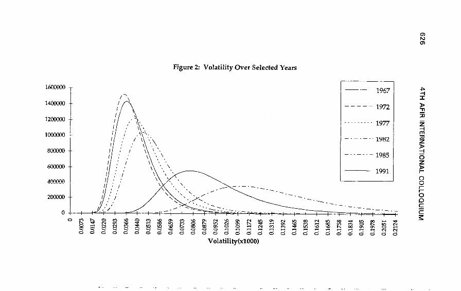
Figure 2: Volatility Over Selected Years
U5OOOOO
1400000
12ooGQo
1OOOOOO
8OOMJO
4oDooo
200000
0
1967
- - 1972
_ _ _ _ _ _ 1977
---.-_. 1982
-..-_.- 1985

MODELING AND MEASURING VOLATILITY
distribution. For year 1991, the posterior distribution is similar to the prior distribution. For
the recession year of 1982, the posterior distribution is very thick tailed and has mass
concentrated at large values of 0’. Therefore, uncertainty in market volatility was smaller in
years 1967, 1972,1977 and 1985 as compared to 1991. In 1991, on average, stock prices did not
contribute any information to reducing uncertainty in market volatility. In 1982, uncertainty in
market volatility was increased after observing market prices. This analysis supports the
observation that uncertainty in market volatility is smaller during periods of high market
returns (bull markets) and larger during recessionary years when returns are not as great.
The third diagram illustrates posterior distributions of market volatility during and
immediately following the stock market crash of 1987. Comparing Figure 2 to Figure 3,
volatility during the stock market crash is 10 to 100 times greater than volatility observed
during a typical year. Even during the year 1982, the average mode of market volatility is only
1.12 x10⁴ compared to 3.95~10~~ on October 19, 1987. There is an increase in market
uncertainty in the week proceeding the crash but it is not significant enough to indicate an
impending market collapse. Figure 3 also shows an improvement in market uncertainty two
weeks after the market failure but it is still significantly larger than compared to the prior’s
uncertainty.
This example also illustrates one of the weaknesses of this model. Since volatility is
assumed constant over an interval of 10 days, there is no distinction made in the calculations on
the order in which market returns are observed. That is, on October 28 and October 30, these
calculations would have produced the same graphs if the market crash occurred on October 19 or
October 27!

628 4TH AFIR INTERNATIONAL COLLOQUIUM
L’ISP’TT
s99om
EIL9’01
09Lz’Ol
8088'6
9SSV.6
E060'6
7’269’8
666C8
9voo6’L
P6Os'L
ZVII’L
06IL’9 =
LEZE’9 5
S8Z6'S $
EEES’S ii YG
08ET'S 5
8ZP.LP
9LLPE’P
EZSKE
ILSS’E
6191-E
999L’Z
PUE’Z
Z9K1
608~T
LS8T'Z
SO6.L0
ZS6E'O
0

MODELING AND MEASURING VOLATILITY 629
6. Conclusion
The Black-Scholes option formula is today one of the most widely used formulae by
market analysts. Unfortunately, stock volatility, which plays an integral part in this
equation, is a difficult parameter to estimate.
The same model that sets the foundation for the Black-Scholes formula is used to
derive a statistical model for the underlying stock volatility. For various reasons, the
likelihood equation is analyzed using a Bayesian statistical approach. First, the market
analyst will be able to incorporate his/her subjective beliefs of market volatility into the
model through the specification of a prior distribution. The prior distribution, although
requiring the specification of five hyperparameters, can be determined indirectly from certain
natural characteristics of the model.
Second, graphing of the posterior distribution allows one to visually interpret
uncertainty in market volatility. During periods of market uncertainty, the posterior
distribution is thick tailed with a large mean (mode). Shifts in the posterior distribution
represent changes in uncertainty of market volatility.
Third, since volatility is constantly changing, little data is available during any
specific time period for an accurate estimate. This would make any large sample estimates
that do not accurately model these changes in volatility inaccurate and therefore, not very
useful.
Finally, uncertainty in market volatility is directly incorporated into the Black-
Scholes model through the posterior distribution. Rather than substituting point estimates into
the formula, the volatility is treated as a random variable. The expected value of the call
option formula is found using the posterior distribution of market volatility. Compared to point
estimates, this approach produces option prices that more closely reflect observed values.

630 4TH AFIR INTERNATIONAL COLLOQUIUM
Acknowledgments
The author would like to thank Dr. W. S. Jewell for helpful suggestions and Dr. M.
Rubinstein for providing the S&P 500 data. Financial support for this research was provided
by Natural Sciences And Engineering Research Council of Canada.
References
Abramowitz, M. and I. A. Stegun (1965). Handbook of Mathematical Functions, New York: Dover Publication, Inc.
Black, F. (1976). Studies of Stock Price Volatility Changes, Proceedings of the 1976 Meeting of Business and Economic Statistics Section, American Statistical Association, 177-181.
Black, F. and M. Scholes (1973). The Pricing of Options and Corporate Liabilities, Journal of Political Economy 81,637-654.
Bollerslev, T., R. Y. Chou and K. F. Kroner (1992). ARCH Modeling In Finance: A Review of the Theory and Empirical Evidence, Journal of Econometrics 52,5-59.
Bowman, F. (1958). Introduction to Bessel Functions, New York: Dover Publications, Inc.
Chou, R. Y. (1988). Volatility Persistence and Stock Valuations: Some Empirical Evidence Using GARCH, Journal of Applied Econometrics 3,279-294
COX, J. C. and C. Huang (1989). Option Pricing Theory and Its Applications, in Bhattacharya and Constantinides eds.
Cox, J. C., J, E. Ingersoll and S. A. Ross (1985). An Intertemporal General Equilibrium Model of Asset Prices, Econometrica 53,363-384.
Fama, E. F. (1981). Stock Returns, Real Activity, Inflation and Money, American Economic Review 70, 839-847.
Hull, J. and A. White (1987). The Pricing of Options on Assets with Stochastic Volatilities, Journal of Finance 42,281-300.
Hull, J. and A. White (1988). An Analysis of the Bias in Option Pricing Caused by a Stochastic Volatility, Advances in Futures and Options.

MODELING AND MEASURING VOLATILITY
Johnson, N. L. and S. Kotz (1970). Continuous Univariate Distributions - 1. Distributions in Statistics, New York: John Wiley & Sons.
Jorgensen, B. (1982). Statistical Properties of Generalized Inverse Gaussian Distribution. Lecture Notes in Statistics, 9, New York: Springer-Verlag.
Malkiel, B. (1979). The Capital Formation Problem in the United States, Journal of Finance 34, 291-306.
Merton, R. C. (1973). Theory of Rational Option Pricing, Bell Journal of Economics and Management Science 4,141-183.
Merton, R. C. (1976). Option Pricing When Underlying Stock Returns are Diicontinuous, Journal of Financial Economics 3, 125-144.
Modigliani, F. and R. Cohn (1979). Inflation, Rational Valuation and the Market, Financial Analyst Journal 35, 3-23.
Pindyck, R. S. (1984). Risk, Inflation and the Stock Market, American Economic Review 74,335- 351.
Press, W. H., B. P. Flannery, S. A. Teukolsky and W. T. Vetterling (1988). Numerical Recipes in C. The Art of Scientific Computing, Cambridge: Cambridge University Press.
Randolph, W. L. (1991). Use of the Mean Reversion Model in Predicting Stock Market Volatility, Journal of Portfolio Management, Spring, 22-26.
Relton, F. E. (1965). Applied Bessel Functions, New York: Dover Publications, Inc.
Wiggins, J. B. (1987). Option Values Under Stochastic Volatility: Theory and Empirical Estimates, Journal of Financial Economics 19,351-372.