MODELING AND DESIGN OF INNOVATIVE SMALL DIAMETER GRAVITY …

162

INTRODUCTION

The small diameter gravity sewerage system (SDGSS) is an alternative to the conventional sanitary gravity sewerage system. It is applied in areas with low population density, high ground water levels and undulating or flat terrains. Un-der such conditions the system may be nearly twice cheaper to build than a conventional one [Błażejewski and Skubisz 2005]. In the SDGSS, septic tanks (STs) with effluent screen filters re-duce the amount of suspended solids getting to the network. In addition, in some cases check valves are used, to prevent backflow of wastewa-ter to the STs and inflow of air to the network. The pipe diameter of service lateral can be as small as 25 mm and the collection main diameter is rang-ing from 50 mm to 100 mm.

The pipes can be laid parallely to the ground surface, even with a negative slope (variable grade effluent sewers) under condition, that the hydraulic head will be smaller than the differ-ence in elevation levels between inlets to the net-work from STs, and the outlet of the network to its final destination. When sewer lines run con-stantly downhill, the system is called a minimum grade effluent sewers.

The SDGSS was developed 50 years ago in Australia. This is still the country where it is the most popular comparing to the rest of the world. It serves there over 110 000 inhabitants [Palmer et al. 2010]. It is also known in the USA and Canada. It seems that one of barriers of the SDGSS further development is a lack of specialized computer codes for its hydraulic design. Existing guidelines for the system design are based mainly on years

MODELING AND DESIGN OF INNOVATIVE SMALL DIAMETER GRAVITY SEWERAGE SYSTEM

Tadeusz Nawrot1, Ryszard Błażejewski1, Radosław Matz1

1 Department of Hydraulic and Sanitary Engineering, Poznan University of Life Sciences, Piatkowska St. 94A, 60-649 Poznan, Poland, e-mail: [email protected]

Journal of Ecological EngineeringVolume 18, Issue 3, May 2017, pages 162–173DOI: 10.12911/22998993/70181 Research Article

ABSTRACT The article presents modern methods of hydraulic design of an innovative small di-ameter gravity sewerage system. In this system, domestic wastewater is preliminary treated in septic tanks equipped with outlet filters, thus the effluent features are similar to those of clear water. Innovative non-return valves at the outlets eliminate introduc-tion of air to the system and thus the flows can be treated as one-phase ones. Computer codes EPANET 2 and SWMM 5.0 were applied and compared. Two flow schemes typical for the sewerage system were implemented in EPANET 2, and the third – in a slightly modified SWMM 5.0. Simulation results were validated on empirical data ob-tained on a laboratory physical model, consisting of four tanks of minimum volumes 600 dm3 each, connecting PE pipelines of diameters 25 mm and 36 mm and relevant sanitary fittings. Water inflows, typical for domestic wastewater outflows from single homesteads, were provided by a pump. Water flows were measured using water me-ters with pulse outputs, and water levels in tanks by pressure transducers. Hydrau-lic characteristics of filters and non-return valves were provided. Simulation results showed good agreement with the empirical data. Ranges of values of design param-eters, needed for successful application of both codes, were established and discussed.

Keywords: small diameter gravity sewerage, mathematical model, hydraulic calculations, EPANET, SWMM

Received: 2017.03.06Accepted: 2017.04.04Published: 2017.05.02

163

Journal of Ecological Engineering Vol. 18(3), 2017

of experience, and therefore they are very differ-entiated. For example, the self-cleansing velocity is given as: 0.5 m∙s-1 by Otis and Mara [1985]; 0.3–0.45 m∙s-1 by Bowne et al. [1991]; 0.2 m∙s-1 by Kreissl et al. [2008]; 0.15 m∙s-1 by Dias and Matos [2001]; and even zero by Little [2004]. These values are mostly empirical; only Dias and Matos [2001] have determined the cleansing ve-locity on the basis of particle size of suspended solids reaching the SDGSS network from a ST, however they considered mineral grains only.

Another uncertain parameter is the design flow. Kreissl et al. [2008] proposed to use the maximum hourly flow, like for the conventional gravity sewers. Canadian guidelines [Ontario Min. 2008] for SDGSS recommend a value of PFh = 2, which is considerably lower than val-ues for conventional gravity sewers (PFh = 4–6 ). According to Crites and Tchobanoglous [1998], hourly peak flow for calculation of alternative sewer systems can be obtained from:

13max min,9.176 dmNQh (1)

and the design peak flow can be calculated as:

NQQ

PFd

hh

max

max1440 (2)

where: Qh max – maximum design peak flow, dm3 ∙ min-1,

N – number of contributing EDUs (equiv-alent dwelling units), EDU,

Qd max – maximum daily wastewater out-flow from 1 EDU, dm3 ∙d-1∙EDU-1 .

Substituting equation (1) into equation (2) and assuming Qd max = 1.2 m3 ∙d-1 ∙ EDU-1 (e.g. 4 persons ∙ 300 dm3 ∙ cap-1 ∙ d-1 ), we obtain:

NN

NNPFh

28.22.911200

)9.176(1440

(3)

On the basis of equation (3) the hourly peak factor will be equal to PFh = 11.4 for N = 10 and for N = 1000 PFh = 2.37 only. This shows how important is to determine the peak flows, espe-cially for initial sections of the network.

Another formula recommended by the USE-PA [1988] to calculate the design flow in systems without storage reads:


The peak flows are significantly attenuated by storage, e.g. in STs. Some constructions of STs were provided with a special last chamber (in-terceptor) with a small orifice (Ø 6 mm) in the outlet pipe to obtain small outflow rates in the range 0.025–0.06 dm3∙s-1.The design peak flow for this system can be calculated from the follow-ing equation by Simmons and Newman [1985]:


The hourly peak factor changes versus the number of contributing EDUs are shown in fig. 1. The value 1.5 in eq. (5) corresponds to the maxi-mum outflow from one dwelling equal to 0.025 dm3∙s-1. Recently, water usages and wastewater discharges are much smaller than 30–40 years ago in the USA. In Polish rural areas it is typically twice less, i.e. maximum 150 dm3∙cap-1∙d-1 instead of the above assumed 300 dm3∙cap-1∙d-1.

During operation of SDGSS at the maximum hydraulic loads, a flooding of the unfavorably located STs, when emptying the preferably lo-cated STs, may occur. Thus, the designer must check the backflow condition in every service lateral. Additionally, minimum once per day the self-cleansing velocity should be provided. For these reasons it was necessary to create a hy-draulic model describing the wastewater flow in SDGSS. Two schemes based on the EPANET 2.0 computer code and one on the SWMM 5.0 were analyzed. The first scheme (A) assumes the full pipe flow at pressurized and quasi-steady flow conditions of wastewater. The second (B) differs from the first one in the possibility to simulate an emptying of the service lateral. The third scheme (C) in turn, allows additionally a simulation of unsteady wastewater flow in partially full pipes (service laterals and mains). Application of EPA-NET code to hydraulic design of pressure sewers is straightforward and relatively easy, as well as

Figure 1. Hourly peak factor depending on the num-ber of contributing EDUs


164

the usage of SWMM to design conventional sani-tary gravity sewers. However, application of these world-wide popular codes to the SDGSS design is not so obvious. The main purpose of this work was to adapt the codes to different schemes of the SDGSS. Results of our efforts were checked on physical lab models.

MATERIALS AND METHODS

Experimental set-up

The experimental set-up used to verify the hy-draulic models implemented in the program EPA-NET 2.0 was consisted of four tanks (Fig. 2), made of PE, of volume 600 dm3, imitating septic tanks.

The tanks were supplied with water. Pressure transducers to measure water levels in the tanks were installed. At the inflow and outflow of each tank, as well as at the outflow from the experi-mental set-up, pulse water meters were provided

with accuracy 1.0 and 2.5 dm3 per pulse, respec-tively. All water meters and pressure transduc-ers were connected to a recorder and controller. The measurement data were recorded with a time step equal to 1 s.

At the 1/3 of the tank height an innova-tive float-ball valve (Fig. 3) was installed. This valve was consisted of a cylindrical float, made of polystyrene, combined with a ball serving as a plug. The ball in the valve was placed be-tween two seats. At the initial phase, the ball laid on the bottom seat, closing the outflow from the tank. With increasing water level in the tank, the float raised up pulling the ball and opening the outlet. In case of a backflow, the ball moved up to the top seat, closing the outflow and inflow (backflow) to the tank.

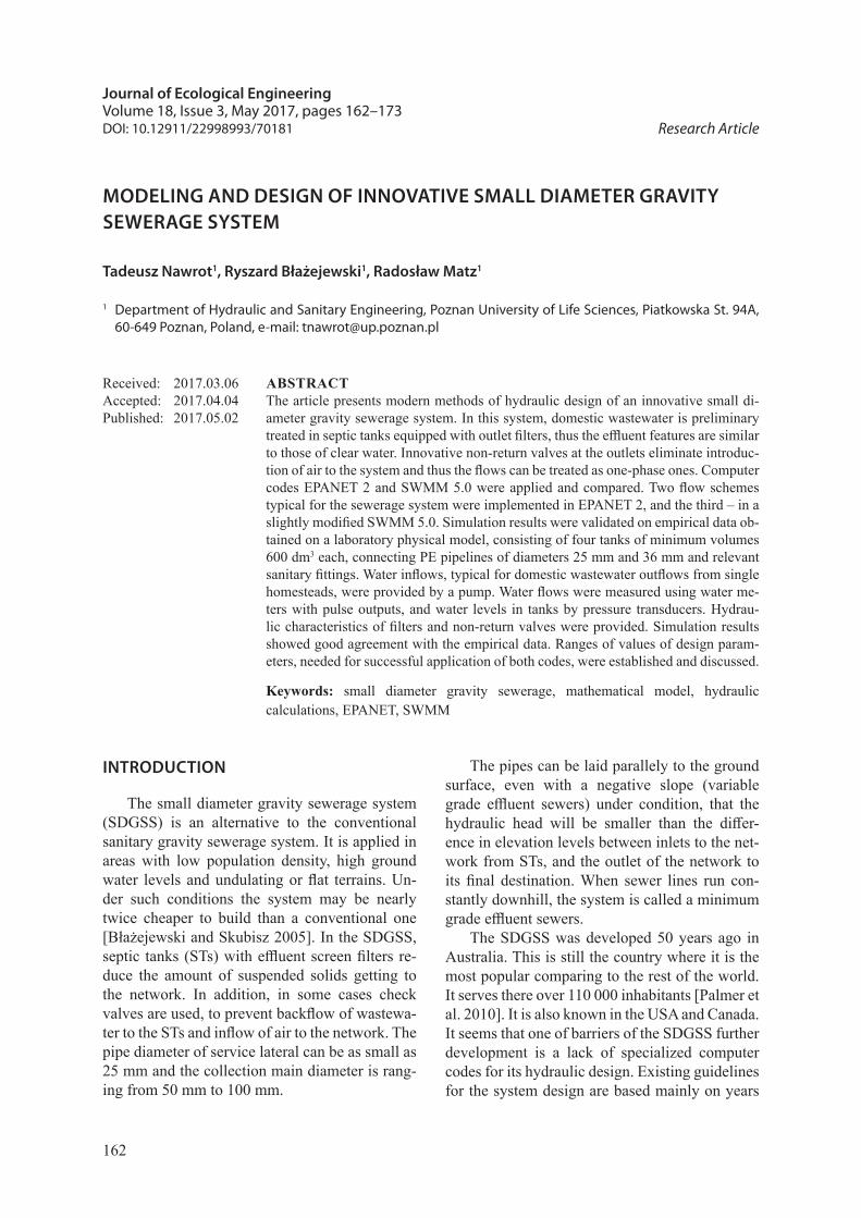
To verify the model C implemented in the SWMM, two connected tanks (Fig. 4) were used. Both tanks were connected by a PE pipe of di-ameter 25 mm. The terminal part of the pipe was made of acrylic glass to make photographs during

Figure 3.Vertical cross section and side view of float-ball valve (dimensions in mm)

Figure 2. Layout of the laboratory installation (all dimensions in mm)

165


the emptying of the upper tank. Basing on analy-sis of the images, the filling of the pipe at the inlet to the bottom tank was evaluated. Frequent auto-matic measurements of water level in the latter tank, allowed for estimation of water flow rate.

Hydraulic models

Hydraulic models implemented in the EPA-NET 2.0 and SWMM 5.0 codes did differ in the complexity of hydraulic calculations. Hydraulic schemes of the SDGSS are shown in figure 6.

The model A has simulated the flow of waste-water with completely filled service laterals and mains (fig. 5a). The condition of completely filled pipe was fulfilled by the float-ball valves acting as check valves and preventing inflow of air into the network. Such a solution reduces the nuisance of odors in a real network, and hydraulic calcula-tions are relatively easy.

Unfortunately, the use of the float-ball valve generates sometimes high vacuum in the network and some troubles with opening due to suction of the ball by the vacuum.

The model B has simulated the wastewater flow in completely filled mains only and has al-lowed emptying the service laterals. In this model the ball-float valves were provided to avoid back-flow of wastewater from the network to ST. The float-ball valves could be replaced in this variant by ordinary check valves. Complete filling the mains can be achieved by inverted siphons (Fig. 5b and 5c). The advantages of such a system are: the absence of vacuum in the network, reliability and ease of hydraulic calculations. The disadvantages are: a higher risk of odor producing and accumula-tion of sediments in the lowest part of mains.

The model C, which hydraulic scheme is shown in figure 5d, simulates wastewater flow at partially filled service laterals and mains. The float-ball valves are not necessary; only in the unfavorably located STs ordinary check valves are used. Thanks to this simplification no vacu-um in the network appear and the risk of sedi-ments’ accumulation is much lower than in the former system. It is also less vulnerable to gen-eration of odors, but the hydraulic calculations are rather sophisticated.

Hydraulic models implemented in the EPANET 2.0

Models, implemented in the EPANET 2 code, allow to calculate flow rates and average veloci-ties in every link of the SDGSS network, pressure heads in all nodes as well as the level of wastewa-ter in each ST. The code simulates steady states, but they can be changed every minute, so one can track the behavior of investigated sewerage system in time. To solve the system of nonlinear equations the gradient method by Todini and Pi-lati was applied [Rossman 2000].

The code distinguishes junctions represent-ed as nodes with unknown pressures in a given time step, and tanks and reservoirs with a steady pressure in a given time step. In the applied modification of the EPANETs code named EPA-NET – Inkano, the STs were simulated using the tanks. In the properties of the tank the invert el-evation level of the outflow pipe from the ST was taken as the “bottom” of the tank, and the maxi-mum height in the tank as the difference between levels of inverts of the inflow and outflow pipes. In addition, in the field volume curve a function

Figure 4. Scheme of installation used to verify the model implemented in the SWMM


166

describing changes of wastewater volume in the active retention part of the ST depending on the filling was entered. Inflows of the raw wastewater into the ST was implemented through the use of junctions with a negative sign. At junctions any hydrographs of wastewater inflow to the network can be set. Outlet from the SDGSS was simulated as a reservoir, for which in the field elevation, the outlet level was introduced.

The float-ball valves (Fig. 4), effluent screen filter and water meters were simulated using the valve function, for which head loss characteris-tics depending on the flow regime (Fig. 6 and 7) were determined in lab by Nawrot [2011]. For float-ball valves and effluent screen filters ap-plied in a given network in the properties of the valve a GPV valve type (called general purpose valve) was set, which generates head losses de-pending on the flow rate. Then, in the settings of the connections, a label describing characteristics of each float-ball valves and effluent screen fil-

ters were entered. In the properties of connection, serving service laterals their status was set as CV (check valve) to eliminate the backflow. The head losses in the SDGSS network were calculated by Darcy-Weisbach method, in which the friction factor was estimated by the Colebrook-White formula. The roughness was assumed equal to k = 0.01 mm. Values of minor loss coefficients are given in Table 1.

Additionally, in order to avoid computational instability a set of rules to control each float-ball valve was implemented. The maximum closing level of wastewater in a ST was taken at 0.0001 m above the height of the invert of outlet from the ST and the minimum opening level was assumed 0.003 m higher than the outlet invert. This has also reflected adequately pulse operation of the valve.

To simulate additionally the emptying (at least partial) of the service laterals, they were treated as tanks in cases when the wastewater levels in relevant STs were close to their outlet

Figure 5. Hydraulic schemes of SDGSS: a) pressurized system simulated in EPANET 2.0 as model A, b-c) surcharged systems simulated in EPANET 2.0 as model B, d) free-water-surface system simulated in SWMM 5.0 as model C; Legend: 1 – septic tank, 2 – effluent screen filter, 3 – float-ball valve, 4 – service lateral, 5 –

collection main

167


invert levels. The difference between the A and B models lies in application of a connections’ bypass, by using a tank for which the character-istics of changes in the volume of water in the service lateral, depending on the filling HSL were assigned (Fig. 8). In this case flow takes place ini-tially through the fully filled service lateral. At the moment when wastewater in the ST has reached its minimum closing level, the flow through the service lateral was closed and an alternative flow through the bypass – a tank simulating service lat-eral. In this case emptying of the service lateral was simulated. During this time, it was possible to add wastewater to the service lateral (tank), if the wastewater level had risen in the ST. When

the maximum filling HSLmax of the “tank” was reached, the bypass was closed and the service lateral was reopened. Conditions of opening and closing a bypass and a ST were implemented as a RULE-BASED algorithm (Fig. 9).

Hydraulic model implemented in the SWMM 5.0

The model C implemented in the program SWMM 5.0 allows to calculate flows, veloci-ties, pipe fillings, in all sections of the SDGSS and to simulate retention in the tank and chan-nels. The program SWMM 5.0 is used mainly for modeling conventional sanitary gravity sewerage system and stormwater drainage, but

Table 1. Minor loss coefficients of elements of the installation as in Fig. 2 acc. to Rossman [2000]

LinkKnee Tee (lateral) Tee (main) Reduction

57/36 mm* Elbow Sharp-edged exit

ξ No. Σξ No. ξ No. ξ No. ξ ξ No. Σξ No. ξS. lateral 1 0.9 3 2.7 1 1.8 0 – 0 – 0.6 18 10.8 0 –S. lateral 2 0.9 3 2.7 1 1.8 0 – 0 – 0.6 14 8.4 0 –S. lateral 3 0.9 3 2.7 1 1.8 0 – 0 – 0.6 10 6.0 0 –S. lateral 4 0.9 3 2.7 1 1.8 0 – 0 – 0.6 6 3.6 0 –C. main 1 – 0 – 0 – 1 0.6 0 – – 0 – 0 –C. main 2 – 0 – 0 – 1 0.6 0 – – 0 – 0 –C. main 3 – 0 – 0 – 1 0.6 0 – – 0 – 0 –C. main 4 – 0 – 0 – 1 0.6 1 0.24 – 0 – 0 –C. main 5 0.9 6 5.4 0 – 1 0.6 0 – – 0 – 1 1.0

* according to Allen and Ditsworth [1972]

Figure 6. Pressure loss in effluent screen filter depending on flow rate [Nawrot 2011]

Figure 7. Pressure loss in float-ball valve with seats of diameter 25 mm depending on flow rate [Nawrot 2011]


168

after small modifications it can also be used for modeling the SDGSS. For hydraulic calcula-tions this code uses a set of one-dimensional Saint-Venant equations in the form a steady flow and kinematic or dynamic wave [Rossman 2010]. In this study the dynamic wave version for model C was applied.

The basic elements of any SWMM’s network are nodes (junction) and tanks (storage unit). The nodes in the program simulate manholes with their specific cross-sectional areas. In the SDGSS

the manholes are replaced by cleanouts. These are tees with exit pipes at the land surface in order to access for periodic cleaning. Therefore, nodes in the model C were implemented as storage units of constant cross-sectional areas. The ST of par-allelepiped or cylindrical shapes can be modeled similarly. However, STs with complex shapes the horizontal cross-sectional area versus the filling height. Head losses on the effluent filter or float-ball valve were introduced as products of minor loss coefficient and relevant velocity head.

Figure 9. Block diagram of the opening and closing of bypass simulating service lateral

Figure 8. Sketch diagram of model B showing wastewater outflow from ST and service lateral simulated as a tank

169


Goodness-of-fit measures

The results obtained from measurements on the experimental setup and from hydraulic mod-els were subjected to statistical analysis. For this purpose, the following measures of conformity with the prototype were used: • coefficient of variation of the root-mean-

square deviation (RMSD)

21

1

2,,

11)(

n

iisim

m

zznz

RMSDCV (6)

• ratio of mean values1 ms zzRoM (7)

• correlation coefficient

sm

smsm zzzzR

(8)

where: n – sample size, zm – the measured value,

zs – the simulated value, z – top bar denotes arithmetic mean, σ – standard deviation.

The best results are to be achieved when CV → 0 as well as RoM and R → 1.0.

RESULTS AND DISCUSSION

In order to check the quality of the models implemented in the EPANET 2, the data obtained from the experimental set-up during the simulta-neous emptying all tanks filled to their maximum level were used.

The measured hydraulic heads in each tank and those derived from the model A are shown in figure 10. It can be seen a good agreement of the calculated and the measured ones. The conver-gence of the measured values with the values of model A was statistically proven (Tab. 2). Some small differences in the cases of tanks 3 and 4 may result from uncertain hydraulic characteris-tics of the float-ball valves. The valve ball can be

Table 2. Statistical measures of mathematical model A quality concerning hydraulic heads in tanks and outflow from the tanks

Statistical measures CV(RMSE) RoM RHydraulic head in tank 1 0.004 0.999 0.997Hydraulic head in tank 2 0.011 1.006 0.982Hydraulic head in tank 3 0.030 1.021 0.960Hydraulic head in tank 4 0.037 0.967 0.986Outflow from tank 1 0.585 0.961 0.834Outflow from tank 2 0.621 0.927 0.770Outflow from tank 3 0.837 0.985 0.462Outflow from tank 4 0.646 1.032 0.740Outflow from experimental set-up 0.279 0.966 0.805

Figure 10. Measured (solid lines) and generated by the model A (dashed lines) hydraulic heads in tanks during their simultaneous emptying


170

set in various positions and that in turn affects its hydraulic resistance.

Rates of outflow from the tanks and instal-lation during simultaneous emptying the tanks, measured and generated by the model A are shown in Figure 11. The initial discrepancy was resulted from the fact of placing water meters at the end of the service laterals. Later on the simulated val-ues of the outflow rates from the entire installa-tion were consistent with the measured values to the moment when the check valve located at the outlet from the 4th tank was temporarily blocked. Nevertheless, taking into account goodness-of-fit measures shown in Table 2, the calculated flow are unsatisfactory . These differences may result from the assumption of completely filled pipe-lines, as well as the quasi-steady flow and the im-possibility of emptying and filling the network. In fact we have observed an unsteady flow.

Pressure head in the tanks simulated using the model B were the same as using model A. This follows from the fact that these models differ only in the possibility to simulate an emptying of the connection, which does not change values of the pressure head in the tanks, but only the values of the wastewater flow rate. Hydraulic heads mea-sured on the experimental set-up and obtained from model B are agreed, which has been statisti-cally proven (Table 4). In terms of the engineer-ing practice, model B is good for determining the hydraulic heads in each tank.

Figure 12 shows values flow on the outflow from the entire installation and from each tank measured and simulated using the model B. Val-

ues obtained from the model B show a greater agreement than those obtained from the model A. In the first period of emptying tanks it is also seen a delay in the intensity of wastewater flow from the network associated with the placement of wa-ter meters at the end of service lateral. In the fur-

Figure 11. Outflow rates from the tanks and installation during simultaneous emptying, measured (solid lines) and generated (dashed lines) by the model A

Table 4. Statistical measures of mathematical model C quality concerning outflow from experimental set-up and water depth measured at the outlet

Statistical measures

Outflow from experimental

set-up

Water depth measured at the

outlet of the experimental

set-upCV(RMSE) 0.215 0.421

RoM 0.967 0.687R 0.937 0.829

Table 3. Statistical measures of mathematical model B quality concerning hydraulic heads in tanks and outflows from the tanks

Statistical measures CV (RMSE) RoM R

Hydraulic head in tank 1 0.005 1.000 0.995Hydraulic head in tank 2 0.011 1.007 0.982Hydraulic head in tank 3 0.031 1.021 0.956Hydraulic head in tank 4 0.030 0.973 0.990Outflow from tank 1 0.661 1.021 0.790Outflow from tank 2 0.806 1.023 0.662Outflow from tank 3 0.940 0.988 0.365Outflow from tank 4 0.682 1.022 0.706Outflow from experimental set-up 0.297 1.003 0.778

171


ther period of the simulation the calculated values have converged to the measured ones. Only in the final period of the simulation the differences have risen. As before, the blockage of the 4th tank’s valve elongated the wastewater outflow from the experimental set-up. Thanks to simulation of emptying of the service laterals these differences were much smaller than in the case of model A. The differences between the values of the outflow from tanks and the experimental set-up measured and simulated by model B (Table 3) seem to be acceptable in engineering practice.

In EPANET 2.0 constant values of the mi-nor loss coefficient were assumed; in reality they change depending on the ratio of flow in various sections of the network. These coefficients did not affect significantly the simulation results, except for the final period of the tanks emptying, when some of them were already empty. In addition, deflection of service lateral pipe sections have occurred in the lab, what would cause additional

head losses or even the air plugs. In reality, simi-lar situations may also occur because of the dif-ficulty with putting down the rolled PE pipeline with a specific constant slope.

The program EPANET 2 allows to implement any of the wastewater inflow hydrograph to the ST. In designing the SDGSS is recommended to choose hourly (peak), and even daily wastewater inflow hydrograph with time step equal to 1 min-ute. After performing simulation of the designed SDGSS one must check whether in all pipes of the network, at least once per day, the minimum self-cleansing velocity is granted.

Water inflow and outflow rates from the net-work measured on the experimental set-up and simulated using SWMM 5.0 are shown in figure 13. The measured and simulated values of the outflow from the installation differ slightly, main-ly due to measurement errors. For the engineering practice, the model C can be described as quite good for outflows from the network (Table 4).

Figure 13. Inflow and outflow rates from the installation during emptying the tank as in Figure 5, measured (step-wise line) and generated by model C

Figure 12. Outflow rates from the tanks and installation during simultaneous emptying, measured (solid lines) and generated (dashed lines) by the model B


172

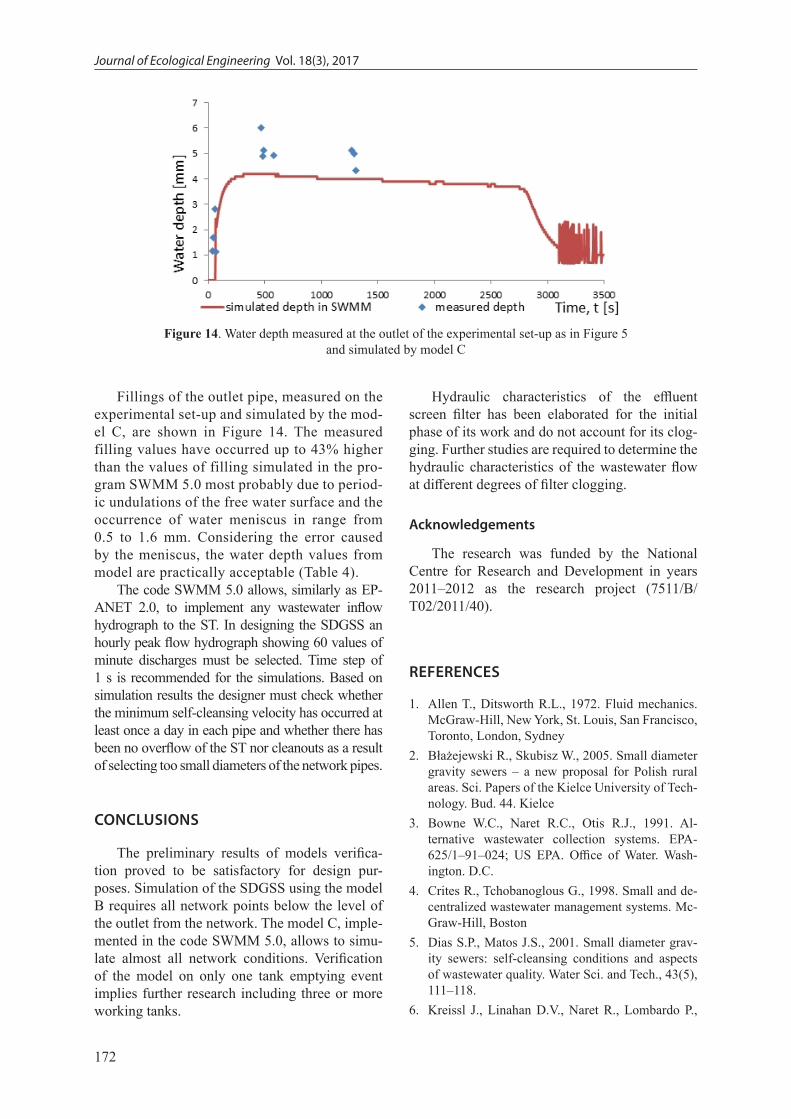
Fillings of the outlet pipe, measured on the experimental set-up and simulated by the mod-el C, are shown in Figure 14. The measured filling values have occurred up to 43% higher than the values of filling simulated in the pro-gram SWMM 5.0 most probably due to period-ic undulations of the free water surface and the occurrence of water meniscus in range from 0.5 to 1.6 mm. Considering the error caused by the meniscus, the water depth values from model are practically acceptable (Table 4).

The code SWMM 5.0 allows, similarly as EP-ANET 2.0, to implement any wastewater inflow hydrograph to the ST. In designing the SDGSS an hourly peak flow hydrograph showing 60 values of minute discharges must be selected. Time step of 1 s is recommended for the simulations. Based on simulation results the designer must check whether the minimum self-cleansing velocity has occurred at least once a day in each pipe and whether there has been no overflow of the ST nor cleanouts as a result of selecting too small diameters of the network pipes.

CONCLUSIONS

The preliminary results of models verifica-tion proved to be satisfactory for design pur-poses. Simulation of the SDGSS using the model B requires all network points below the level of the outlet from the network. The model C, imple-mented in the code SWMM 5.0, allows to simu-late almost all network conditions. Verification of the model on only one tank emptying event implies further research including three or more working tanks.

Hydraulic characteristics of the effluent screen filter has been elaborated for the initial phase of its work and do not account for its clog-ging. Further studies are required to determine the hydraulic characteristics of the wastewater flow at different degrees of filter clogging.

Acknowledgements

The research was funded by the National Centre for Research and Development in years 2011–2012 as the research project (7511/B/T02/2011/40).

REFERENCES

1. Allen T., Ditsworth R.L., 1972. Fluid mechanics. McGraw-Hill, New York, St. Louis, San Francisco, Toronto, London, Sydney

2. Błażejewski R., Skubisz W., 2005. Small diameter gravity sewers – a new proposal for Polish rural areas. Sci. Papers of the Kielce University of Tech-nology. Bud. 44. Kielce

3. Bowne W.C., Naret R.C., Otis R.J., 1991. Al-ternative wastewater collection systems. EPA-625/1–91–024; US EPA. Office of Water. Wash-ington. D.C.

4. Crites R., Tchobanoglous G., 1998. Small and de-centralized wastewater management systems. Mc-Graw-Hill, Boston

5. Dias S.P., Matos J.S., 2001. Small diameter grav-ity sewers: self-cleansing conditions and aspects of wastewater quality. Water Sci. and Tech., 43(5), 111–118.

6. Kreissl J., Linahan D.V., Naret R., Lombardo P.,

Figure 14. Water depth measured at the outlet of the experimental set-up as in Figure 5 and simulated by model C

173


2008. Alternative Sewer Systems – MOP FD-12. 2nd Edition. WEF Press. Alexandria. Virginia

7. Little C.J., 2004. A comparison of sewer reticula-tion system design standards gravity. vacuum. and small bore sewers. Water SA. 30(5), 685–692

8. Nawrot T., 2011. Hydraulic characteristics of septic tank fittings in small diameter gravity sewer systems (in Polish). Nauka Przyr. Technol. 5(5), #91.

9. Ontario Ministry of the Environment, 2008. Clear-ford Small Bore Sewer™ System http://www.clearford.com/SBS/index.shtml

10. Otis R.J., Mara D., 1985. The Design of Small Bore Sewer Systems. United Nations Development Programme. Interregional Project INT/81/047

11. Palmer N., Lightbody P., Fallowfield H., Harvey B., 2010. Australia’s most successful alternative to sewerage: SA’s septic tank effluent disposal schemes. http://www.efm.leeds.ac.uk/CIVE/Sew-erage/articles/australia.pdf

12. Rossman L., 2000. EPANET 2 Users Manual. Cin-cinnati. OH

13. Rossman L., 2010. Storm Water Management Model Version 5.0 Users Manual. Cincinnati. OH

14. Simmons J.D., Newman J.O., 1985. Small-diame-ter, variable grade gravity sewers. Journal (Water Pollution Control Federation), Vol. 57, No. 11

15. USEPA, 1988. Variable Grade Sewers. Special Evaluation Project. Design module 22NSFC.

Documents

MODELING AND DESIGN OF INNOVATIVE SMALL DIAMETER GRAVITY …