Modeling and Control of Z-Source Converter

for Fuel Cell Systems (Technical Report)

Jin-Woo Jung, Ph. D Student Ali Keyhani, Professor

Mechatronic Systems Laboratory Department of Electrical and Computer Engineering

The Ohio State University

Columbus Ohio 43210

Tel: 614-292-4430

Fax: 614-292-7596

keyhani.1@osu.edu

Date: May 03, 2004

TABLE OF CONTENTS

ABSTRACT

I. INTRODUCTION

II. MODELING OF FUEL CELL SYSTEMS

III. CONFIGURATION OF FUEL CELL SYSTEM

IV. CIRCUIT ANALYSIS

V. SYSTEM MODELING

VI. SPACE VECTOR PWM IMPLEMENTATION

VII. SIMULATION RESULTS

VIII. CONCLUSIONS

ACKNOWLEDGEMENT

REFERENCES

APPENDIX

A. MATLAB CODE FOR THE INITIALIZATION BEFORE THE SIMULINK SIMULATION

B. THE SIMULINK MODEL USED IN THE SIMULATION

1

Abstract—This report presents a detailed circuit analysis and PWM implementation of a

fuel cell based Z-source converter using L and C components. The fuel cell system is

modeled by an electrical R-C circuit in order to include a slow dynamics of the fuel cells

and a voltage-current characteristic of a cell is also considered. A discrete-time state space

model of the Z-source converter is given for DSP implementation. A modified space vector

pulse width modulation is described in detail. To verify the effectiveness of the analyzed

circuit model and modified space vector PWM technique, various simulation results using

Matlab/Simulink are presented under a closed-loop control and Matlab/Simulink models

are attached in Appendix. Also, all Matlab/Simulink codes are given.

Index Terms—Z-source converter, boost converter, fuel cells, distributed generation systems.

I. INTRODUCTION

Interest in emerging power generation technologies such as wind turbines, photovoltaic arrays

and fuel cells is rapidly increasing due to global pollution problems [1-7]. The fuel cell systems

can always produce electric power regardless of climate conditions as long as hydrogen and

oxygen are supplied.

A fuel cell is an electrochemical device which converts chemical energy directly to electric

energy by an electrochemical reaction of hydrogen and oxygen. Furthermore, the fuel cell system

produces only electricity, water, and heat, and has 50 % efficiency for only electricity and could

reach 85 % in case of co-generation. Thus, fuel cells are a DC power source of safe, clean, and

efficient electric power generation. Types of the fuel cells are categorized according to the

electrolyte used: Proton-Exchange-Membrane (PEM), Phosphoric Acid (PA), Molten Carbonate

(MC), Solid Oxide (SO), Alkaline, and Zinc-Air (ZA) fuel cells, etc. Also, anticipated

applications of the fuel cells include stationary (buildings, hospitals, etc), residential (domestic

utility), transportation (fuel cell vehicles), portable power (laptop, cell phone) and distributed

power generation.

A detailed dynamic modeling of the fuel cell systems has been presented based on chemical

and physical processes [8-15]. The mathematical model of the reformer and stack is represented

by a simple R-C circuit for a conventional DC-DC boost converter in [16]. Lately, attention is

2

put on design of the Power Electronic interface system that is inexpensive, reliable, small-sized

and light-weighted for residential applications [18-21]. In order to produce higher AC voltage

than the DC output voltage of the fuel cells, the conventional fuel cell systems in these papers

have used a DC/DC boost converter and a DC/AC inverter, and the fuel cells are modeled by a

DC voltage source. In reference [22], a new Z-source converter is proposed that does not need

any boost converter in order to step up a low DC output voltage of fuel cells to a higher DC

voltage and uses the fuel cell modeled by a constant DC voltage source and then analyzed its

operation under an open-loop control.

However, a detailed dynamic model of the fuel cells in conjunction with a detailed circuit of Z-

source converter with PWM implementation has not been studied [22-23]. In this report, we

focus on an electrical analysis of the fuel cell based three-phase PWM inverter with an electrical

R-C circuit model to present the slow dynamic response of a fuel cell. In our analysis, a discrete-

time state space model of the Z-source converter is given for design of a closed-loop control

system using digital signal processor (DSP). To validate the proposed method, simulation studies

are performed for a test bed of an AC 208 V/60 Hz/10 kVA system.

II. MODELING OF FUEL CELL SYSTEMS

Hydrogen gas required for the fuel cell systems to produce DC power is indirectly derived

from a reformer using fuels such as natural gas, propane, methanol, gasoline or from the

electrolysis of water, or can be directly obtained from stored hydrogen or hydrogen pipeline.

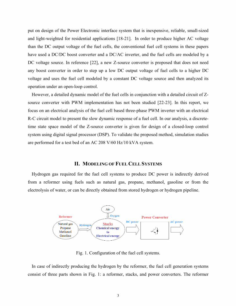
Fig. 1. Configuration of the fuel cell systems.

In case of indirectly producing the hydrogen by the reformer, the fuel cell generation systems

consist of three parts shown in Fig. 1: a reformer, stacks, and power converters. The reformer

3

produces hydrogen gas from fuels and then provides it for the stacks. The stacks have many unit

cells which are stacked in series to generate a higher voltage needed for their applications

because one single cell that consists of electrolyte, separators, and plates, produces

approximately 0.7 V DC. Also it generates DC electric power by an electrochemical reaction of

hydrogen and oxygen. The power converters convert a low voltage DC from the fuel cell to a

high voltage DC or a sinusoidal AC.

Fig. 2. Block diagram of reformer and stacks.

For dynamic modeling of the fuel cells, the reformer and stack are further described because a

dynamic response of the fuel cell systems is determined by them. Fig. 2 shows a block diagram

of reformer and stacks to illustrate their operation. First of all, the reformer that produces the

hydrogen for power generation requested from the load significantly affects dynamic response of

the fuel cell system because it takes several to tens of seconds to convert the fuel into the

hydrogen depending on the demand of the load current. Thus, in order to investigate an overall

operation of fuel cell powered systems, the dynamics of the reformer may be represented as a

simple model like a first order time delay circuit [16] or a second order model [17].

On the other hand, the response of the stacks is considered to much faster respond to

hydrogen from the reformer and oxygen from the air rather than that of the reformer. In Fig. 2,

the output of the stacks shows different voltage-current polarization curves for varying hydrogen

mass flow rate: i.e., the maximum cell current and stack voltage increase as the hydrogen mass

flow rate increases. As a consequence, a dynamic response of the reformer and stacks and a

characteristic of cell current-stack voltage need to be modeled for more realistic analysis of the

fuel cell powered systems.

In this report, a simple R-C circuit model is used to realize slow dynamics caused by a

4

chemical/electrical response of the reformer and stacks [16]. Fig. 3 shows an electrical

equivalent circuit model used for the fuel cells. As shown in Fig. 3, the reformer and stack are

modeled by Rr and Cr, and Rs and Cs, respectively.

Fig. 3. Electrical equivalent circuit model of the fuel cell.

Further, voltage-current characteristic of the stack is considered. Even if the maximum cell

current or stack voltage for each hydrogen flow rate should be represented as a sharp drop of cell

voltage due to primarily starvation of the hydrogen as shown in Fig. 2, the V-I characteristic in

Fig. 4 is used for a simplified circuit model in this study.

Fig. 4. Voltage-current characteristic of a cell.

1. Theoretical EMF or ideal voltage (1.16 V) 2. Region of Activation Polarization (Reaction Rate Loss)

3. Region of Ohmic Polarization 4. Region of Concentration Polarization (Gas Transport Loss)

III. CONFIGURATION OF FUEL CELL SYSTEM

Fig. 5 shows total system diagram of Z-source converter with a fuel cell that consists of a

5

reformer, stacks, a fuel cell processor, a PWM inverter DSP controller, a Z-source converter, and

a load. As illustrated in Fig. 5, the fuel processor controls the reformer to produce hydrogen for

power requested from the PWM inverter DSP controller, and monitors the stack current and

voltage. The PWM inverter DSP controller communicates with the fuel cell processor to equalize

power available from the stack to power requested by the load, and controls the Z-source

converter, and senses output voltages/currents for a feedback control.

Fig. 5. Total system diagram of Z-source converter with a fuel cell.

Fig. 6 shows system configuration with Z-source converter used as power electronic interface

system for fuel cell systems. The filter capacitors (Cf) to eliminate harmonics of the inverter

output voltage due to the PWM technique are added to the conventional Z-source converter. In

Fig. 6, the system consists of a fuel cell, a diode, impedance components (L1, 2 and C1, 2), a three-

phase inverter, an output filter (Lf and Cf), and a 3-phase load. The diode between the fuel cell

and Z-source converter is required to prevent a reverse current that can damage the fuel cell.

The Z-source converter is based on a new concept different from a conventional DC/AC

power converter. In the conventional 3-phase voltage source inverter (VSI), the shoot-through

that both switches in a leg are simultaneously turned on must be avoided because it causes a

short circuit. So the traditional three-phase VSI has eight basic switching vectors that consist of

six active vectors V1-V6 which impress the DC-link voltage on the load and two zero vectors V0,

V7 which do not impress the DC-link voltage on the load. Meanwhile, the Z-source converter has

one more vector (i.e., the shoot-through zero vector) besides eight basic switching vectors. It

6

utilizes the shoot-through in order to directly boost a DC source voltage without a boost DC/DC

power converter because topology of the Z-source converter makes the boost feature stated

above possible. Also, a boosted voltage rate absolutely depends on total duration (Ta) of the

shoot-through zero vectors over one switching period (Tz).

Fig. 6. System configuration with Z-source converter.

IV. CIRCUIT ANALYSIS

To explain the operating principle of the Z-source converter, the equivalent circuit model of

the Z-source converter is shown in Fig. 7 when Fig. 6 is viewed from the DC-link. Fig. 7 (a)

shows the equivalent circuit of the Z-source converter in the shoot-through zero vectors, while

Fig. 7 (b) shows that of the Z-source converter in the non-shoot-through switching vectors.

If we assume that inductor L1 and capacitor C1 are equal to inductor L2 and capacitor C2,

respectively, we can obtain the following equations from one of shoot-through zero vectors and

one of non-shoot-through switching vectors.

VC1 = VC2 and vL1 = vL2. (1)

Case 1: one of shoot-through zero vectors (Fig. 7 (a))

vL1 = VC1, vf = 2VC1, and vi = 0. (2)

7

Case 2: one of non-shoot-through switching vectors (Fig. 7 (b))

loop : vL1 = vf – VC1 = Vin – VC1

loop : vi = VC1 – vL1 = 2VC1 – Vin, (3)

where, Vin is the output voltage of the fuel cell.

(a) (b)

Fig. 7. Equivalent circuit of Z-source converter.

(a) In the shoot-through zero vectors. (b) In the non-shoot-through switching vectors.

We assume that Tz = Ta + Tb, where Tz: switching period, Ta: total duration of shoot-through

zero vectors over Tz, and Tb: total duration of non-shoot-through switching vectors over Tz. If we

use the fact that the average voltage of the inductors over one switching period (Tz) is equal to

zero in steady state, we can obtain the following equation from (2) and (3)

( )

in

z

a

z

a

inab

bC

T

z

CinbCaLLL

V

TT

TT

VTT

TV

TVVTVT

dtvvV z

⋅−

−=

−=⇒

=−⋅+⋅

=== ∫

21

1

0

1

0

11111

. (4)

Also, the average DC-link voltage can be expressed below

8

( )1

10

20Cin

ab

b

z

inCbaT

iii VVTT

TT

VVTTdtvvV z =−

=−⋅+⋅

=== ∫ . (5)

From (5), the average DC-link voltage (Vi) is equal to capacitor voltage (VC1), so the

measured VC1 can be used to regulate the DC-link voltage. Next, we can calculate the peak DC-

link voltage using (3) and (4)

ininab

zinCDCp VKV

TTT

VVV ⋅=−

=−= 1_ 2 , (6)

where, 121

1≥

⋅−=

−=

z

aab

z

TTTT

TK , (7)

K is called a boost factor and is always more than one in order to obtain the boosted DC voltage

compared to the output DC voltage of the fuel cell. Using (6), a peak phase voltage of inverter

output can be written as

22_

_inDCp

paV

KMV

MV ⋅⋅=⋅= , (8)

where, M denotes the modulation index.

Finally, from (8) we can know that the peak phase voltage (Va_p) of inverter output definitely

depends on both the modulation index (M) and the boost factor (K), and from (7) the boost factor

(K) is determined by a ratio Ta/Tz.

( MTT

TTTTT

z

b

z

abaz =+=⇒+= 1 ) . (9)

Moreover, sum of the modulation index (M=Tb/Tz) and the ratio Ta/Tz is always equal to unity

because Tb/Tz is related to the non-shoot-through vectors while Ta/Tz is to the shoot-through zero

vectors as expressed in (9).

9

V. SYSTEM MODELING

Fig. 6 can be simplified as shown in Fig. 8 for an analytic modeling of Z-source converter

with fuel cells. In Fig. 8, the system consists of a DC voltage source (Vdc), a three-phase inverter,

an output filter (Lf and Cf), and a 3-phase load. Note that a fuel cell, a diode (D), and impedance

components (L1, 2 and C1, 2) are replaced with a DC-link voltage source (Vdc) for circuit

modeling, and Vdc is also equal to the average DC-link voltage VC1 or VC2.

Fig. 8. Simplified circuit model of Z-source converter.

The simplified circuit model described in Fig. 8 uses the following quantities. The inverter

output line-to-line voltage is represented by the vector Vi = [ViAB ViBC ViCA]T. The inverter output

currents are iiA, iiB, and iiC. From these currents, a vector can be defined as Ii = [iiAB iiBC iiCA]T =

[iiA−iiB iiB−iiC iiC−iiA]T. Also, the load line to line voltage and phase current vectors can be

represented by VL = [VLAB VLBC VLCA]T and IL = [iLA iLB iLC]T, respectively.

On the L-C output filter, the following current and voltage equations are derived:

i). Current equations:

( )

( )

( )⎪⎪⎪

⎩

⎪⎪⎪

⎨

⎧

−−=

−−=

−−=

LALCf

iCAf

LCA

LCLBf

iBCf

LBC

LBLAf

iABf

LAB

iiC

iCdt

dV

iiC

iCdt

dV

iiC

iCdt

dV

31

31

31

31

31

31

, (10)

10

ii). Voltage equations:

⎪⎪⎪

⎩

⎪⎪⎪

⎨

⎧

−=

−=

−=

LCAf

iCAf

iCA

LBCf

iBCf

iBC

LABf

iABf

iAB

VL

VLdt

di

VL

VLdt

di

VL

VLdt

di

11

11

11

. (11)

Rewrite (10) and (11) into a vector form, respectively:

Lf

if

i

Lif

if

L

LLdtd

CCdtd

VVI

ITIV

113

13

1

−=

−=

. (12)

where, . ⎥⎥⎥

⎦

⎤

⎢⎢⎢

⎣

⎡

−−

−=

101110

011

iT

For implementation of SVPWM, the three-phase system represented by the above state

equations can be transformed to a stationary qd reference frame that consists of the horizontal (q)

and vertical (d) axes. The mathematical relationship between these two reference frames is

abcsqd fKf =0 , (13)

where, ⎥⎥⎥

⎦

⎤

⎢⎢⎢

⎣

⎡−−−

=2/12/12/1

232302/12/11

32

sK , fqd0=[fq fd f0]T, fabc=[fa fb fc]T, and f denotes either a voltage or a

current variable.

Rewrite (12) in the stationary qd reference frame below:

11

Lqdf

iqdf

iqd

Lqdiqdf

iqdf

Lqd

LLdtd

CCdtd

VVI

ITIV

11

31

31

−=

−=

, (14)

where, Tiqd = [KsTiKs-1]row, column, 1,2 =

⎥⎥⎥⎥

⎦

⎤

⎢⎢⎢⎢

⎣

⎡ −

13

13

11

23 .

Thus, assuming the parameters of all passive components are constant, the given plant model

can be expressed as the following continuous-time state space equation for a linear time-

invariant (LTI) system

)()()()( tttt EdBuAXX ++=& , (15)

where,

14×

⎥⎦

⎤⎢⎣

⎡=

iqd

Lqd

IV

X ,

44

2222

2222

013

10

×

××

××

⎥⎥⎥⎥

⎦

⎤

⎢⎢⎢⎢

⎣

⎡

−=

IL

IC

f

fA ,

24

22

2210

×

×

×

⎥⎥⎥

⎦

⎤

⎢⎢⎢

⎣

⎡= I

L f

B , , [ ] ⎥⎦

⎤⎢⎣

⎡==

×id

iqiqd V

V12

Vu

242203

1

×× ⎥⎥⎥

⎦

⎤

⎢⎢⎢

⎣

⎡−= iqd

fCT

E , . ⎥⎦

⎤⎢⎣

⎡== ×

Ld

LqLqd i

i12][Id

Notice that the line to line load voltage VLqd and inverter output current Iiqd are the state

variables of the system, the inverter output line-to-line voltage Viqd is the control input (u), and

the load current ILqd is defined as the disturbance (d).

For realization of digital control, the (15) can be converted into a discrete-time state space

equation:

)()()()1( *** kkkk dEuBXAX ++=+ , (16)

12

where, , , . zTe AA =* ∫ −= zz

T T de0

)(* ττ BB A ∫ −= zz

T T de0

)(* ττ EE A

The above discrete-time state space plant model (16) can be used for design of a feedback

control system using digital signal processor (DSP) or microcontroller.

VI. SPACE VECTOR PWM IMPLEMENTATION

Most of pulse-width modulation (PWM) schemes can be used for the Z-source converter. In

this report, a space vector PWM technique (SVPWM) is used to implement the Z-source

converter because of less harmonic distortion in the output voltages and more efficient use of

supply voltage.

Fig. 9. Basic space vectors and switching patterns.

For realization of SVPWM, a three-phase voltage or current vector in the abc reference frame

is transformed into a vector in the stationary qd coordinate frame. Fig. 9 shows eight possible

switching vectors of on and off patterns for the three upper power transistors that feed the three-

phase DC to AC inverter. Six non-zero vectors (V1 - V6) forms the axes of a hexagonal, and two

zero vectors (V0 and V7) are at the origin. Also, the vectors divide the plane into six sectors, and

the angle between any adjacent two non-zero vectors is 60 degrees.

13

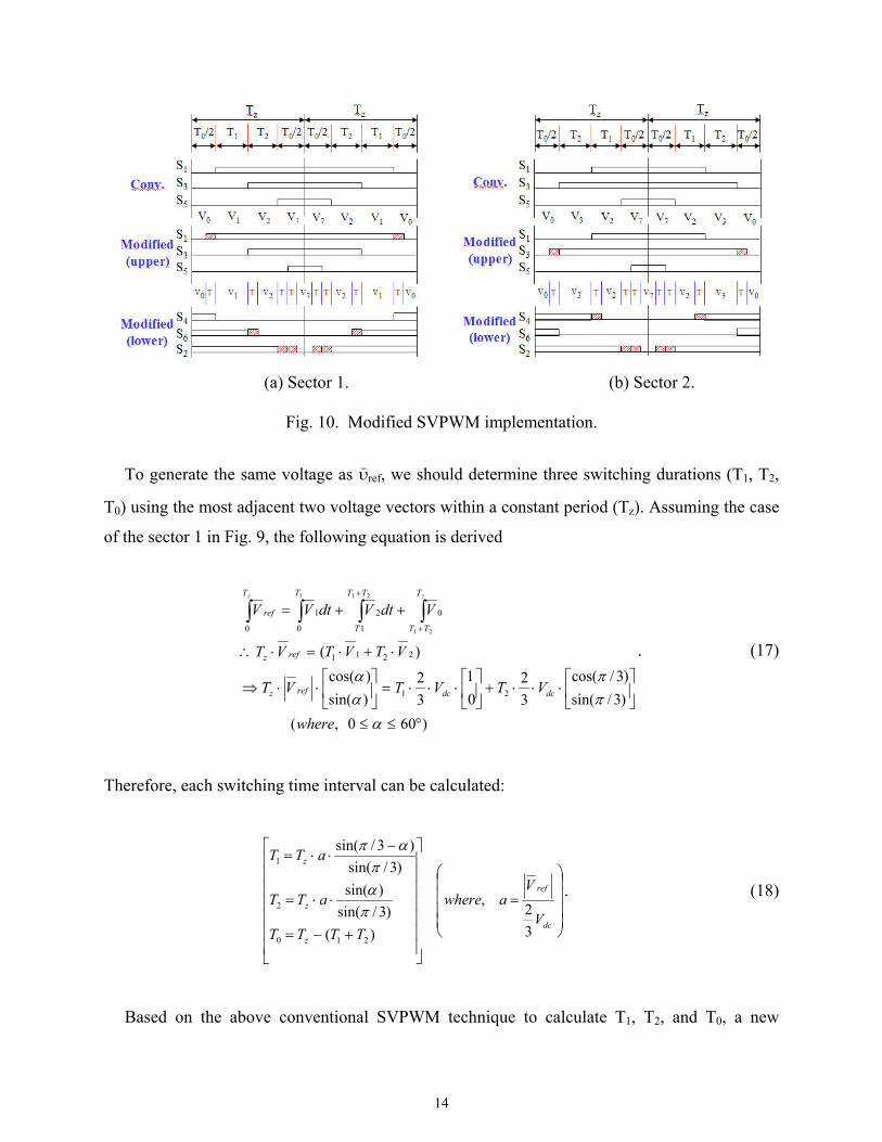
(a) Sector 1. (b) Sector 2.

Fig. 10. Modified SVPWM implementation.

To generate the same voltage as ῡref, we should determine three switching durations (T1, T2,

T0) using the most adjacent two voltage vectors within a constant period (Tz). Assuming the case

of the sector 1 in Fig. 9, the following equation is derived

)600,()3/sin()3/cos(

32

01

32

)sin()cos(

)(

21

2211

0

1

2

0 0

1

21

211

°≤≤

⎥⎦

⎤⎢⎣

⎡⋅⋅⋅+⎥

⎦

⎤⎢⎣

⎡⋅⋅⋅=⎥

⎦

⎤⎢⎣

⎡⋅⋅⇒

⋅+⋅=⋅∴

++= ∫∫∫ ∫+

+

αππ

αα

where

VTVTVT

VTVTVT

VdtVdtVV

dcdcrefz

refz

T

TT

TT

T

T T

ref

zz

. (17)

Therefore, each switching time interval can be calculated:

⎟⎟⎟⎟

⎠

⎞

⎜⎜⎜⎜

⎝

⎛

=

⎥⎥⎥⎥⎥⎥⎥

⎦

⎤

⎢⎢⎢⎢⎢⎢⎢

⎣

⎡

+−=

⋅⋅=

−⋅⋅=

dc

ref

z

z

z

V

Vawhere

TTTT

aTT

aTT

32,

)()3/sin(

)sin()3/sin(

)3/sin(

210

2

1

παπ

απ

. (18)

Based on the above conventional SVPWM technique to calculate T1, T2, and T0, a new

14

duration (T = Ta/3) should be added to the traditional SVPWM in order to boost the DC-link

voltage of the Z-source converter and to generate the sinusoid AC output voltage. As mentioned

in the previous section, the rate of DC-link boosted voltage is determined by the total duration

(Ta) of shoot-through zero vectors that at once turn on both power switches in a leg. Fig. 10

shows both the conventional and modified switching patterns for the Z-source converter at sector

1, 2. In Fig. 10, each phase leg still switches on and off once per switching cycle (Tz), and each

phase has only one shoot-through zero state (T) during one period (Tz) in any sector without any

change of total zero vectors (V0, V7, and T) and total nonzero switching vectors (V1 – V6). Even

if the output voltage of inverter and DC-link voltage can be controlled by adjusting Ta, the

maximum available shoot-through interval (Ta) to boost the DC-link voltage (vi) is restricted by

the zero vector duration (T0/2) which is determined by the modulation index (M = a⋅(4/3)).

TABLE I. SWITCHING TIME DURATION AT EACH SECTOR Sector Upper (S1, S3, S5) Lower (S4, S6, S2)

1 S1 = T1 + T2 + T0 /2 + T S3 = T2 + T0 /2 S5 = T0 /2 − T

S4 = T0 /2 S6 = T1 + T0 /2 + T S2 = T1 + T2 + T0 /2 + 2T

2 S1 = T1 + T0 /2 S3 = T1 + T2 + T0 /2 + T S5 = T0 /2 − T

S4 = T2 + T0 /2 + T S6 = T0 /2 S2 = T1 + T2 + T0 /2 + 2T

3 S1 = T0 /2 − T S3 = T1 + T2 + T0 /2 + T S5 = T2 + T0 /2

S4 = T1 + T2 + T0 /2 + 2T S6 = T0 /2 S2 = T1 + T0 /2 + T

4 S1 = T0 /2 − T S3 = T1 + T0 /2 S5 = T1 + T2 + T0 /2 + T

S4 = T1 + T2 + T0 /2 + 2T S6 = T2 + T0 /2 + T S2 = T0 /2

5 S1 = T2 + T0 /2 S3 = T0 /2 − T S5 = T1 + T2 + T0 /2 + T

S4 = T1 + T0 /2 + T S6 = T1 + T2 + T0 /2 + 2T S2 = T0 /2

6 S1 = T1 + T2 + T0 /2 + T S3 = T0 /2 − T S5 = T1 + T0 /2

S4 = T0 /2 S6 = T1 + T2 + T0 /2 + 2T S2 = T2 + T0 /2 + T

To help understand implementation of the space vector PWM modified for the Z-source

converter, the switching time of the upper switches and the lower switches in a 3-phase inverter

is summarized in Table I. Note that when the shoot-through duration (T) is equal to zero, the

switching time of each power switch for the Z-source converter is exactly the same as that for the

15

conventional one.

VII. SIMULATION RESULTS

In order to verify the effectiveness of the analyzed circuit model and modified SVPWM

implementation, a simulation test bed using Matlab/Simulink is constructed for an AC 208 V (L-

L)/10 kVA, and simulation studies are performed under a closed-loop control. The system

parameters are given in Table II.

TABLE II. SYSTEM PARAMETERS FOR SIMULATIONS Fuel Cell Output Voltage Vin = 150 – 250 V

Desired Average DC-link Voltage VC2 = 360 V Output Rated Power Pout = 10 kVA

Impedance Components L1 = L2 = 200 uH, C1 = C2 = 1000 uF

Inverter Output Filters Lf = 580 uH, Cf = 380 uF

AC Output Voltage VL, RMS = 208 V (L-L), f = 60 Hz

Switching/Sampling Period Tz = 1/(5.4 kHz)

From (7)-(9) and Table II, the parameters K, M, a, and T can be calculated theoretically below

by (19):

i). When Vin = 150 V and P = 10 kW:

Ta/Tz = 0.3684, K = 3.799, M = 0.6316, a = 0.4737,

T = 22.1 µsec.

ii). When Vin = 250 V and P = 5 kW:

Ta/Tz = 0.2340, K = 1.88, M = 0.766, a = 0.5745,

T = 14.44 µsec.

16

3/4/3/1)/(

/211

2/

/21/1

2

1

1

21

a

zazb

zainC

inCza

inza

za

az

az

ab

bCC

TTMaTTTTM

TTK

VVVVTT

VTT

TTTT

TTTT

TVV

=∴⋅=⇒−==∴⋅−

=⇒−⋅−

=∴

⋅⋅−

−=

−−

=−

==

. (19)

150 200 250 300 3500

0.2

0.4

Ta/Tz

Vin

150 200 250 300 3500

2

4

KTa/Tz

K

Fig. 11. Relationship between Vin, Ta/Tz, and K.

From Table II and (19), relationship between Vin, Ta/Tz, and K is shown in Fig. 11. As we

expect, Ta/Tz and K decrease as the output voltage (Vin) of the fuel cell increases.

Fig. 12. Simulink model for an overall system.

17

Fig. 13. Simulink model for a PWM inverter DSP controller.

Based on these calculated parameters, the simulations are implemented under a linear load for

two cases: a load increase and a load decrease. From Fig. 4, when the load increases from 5 kW

to 10 kW, we assume that the output voltage of the fuel cell is changed from 250 V to 150 V. On

the other hand, when the load decreases from 10 kW to 5 kW, the output voltage of the fuel cell

is changed from 150 V to 250 V. In addition, we assume the parameters of the reformer and

stack: Rr = 0.05 Ω and Cr = 42.8 mF, Rs = 0.02 Ω and Cs = 4.2 mF. Fig. 12 shows the Simulink

model for an overall system, while Fig. 13 shows the Simulink model for a PWM inverter DSP

controller which consists of discrete-time PI voltage/current controllers and a DC-link PI

controller.

18

0.0167 0.0168 0.0168 0.0169 0.0169 0.017 0.017 0.0170

1

2

S1

0.0167 0.0168 0.0168 0.0169 0.0169 0.017 0.017 0.0170

1

2

S4

0.0167 0.0168 0.0168 0.0169 0.0169 0.017 0.017 0.0170

1

2

S3

0.0167 0.0168 0.0168 0.0169 0.0169 0.017 0.017 0.0170

1

2

S6

0.0167 0.0168 0.0168 0.0169 0.0169 0.017 0.017 0.0170

1

2

S5

0.0167 0.0168 0.0168 0.0169 0.0169 0.017 0.017 0.0170

1

2

S2

Time [sec]

Fig. 14. Gating signals for six power switches.

0.05 0.055 0.06 0.065 0.07 0.075 0.08 0.085 0.09 0.095 0.10

100

200

300

400

Vin

, VC2

[V]

VinVC2

0.05 0.055 0.06 0.065 0.07 0.075 0.08 0.085 0.09 0.095 0.1-400

-200

0

200

400

VLAB

, VLBC

, VLCA

0.05 0.055 0.06 0.065 0.07 0.075 0.08 0.085 0.09 0.095 0.1-50

0

50

Time [sec]

i LA, i

LB, i

LC [A]

Fig. 15. Simulation results when Vin = 250 V and P = 5kW.

19

0.05 0.055 0.06 0.065 0.07 0.075 0.08 0.085 0.09 0.095 0.10

100

200

300

400

Vin

, VC2

[V]

VinVC2

0.05 0.055 0.06 0.065 0.07 0.075 0.08 0.085 0.09 0.095 0.1-400

-200

0

200

400

VLAB, VLBC, VLCA

0.05 0.055 0.06 0.065 0.07 0.075 0.08 0.085 0.09 0.095 0.1-50

0

50

Time [sec]

i LA, i

LB, i

LC [A]

Fig. 16. Simulation results when Vin = 150 V and P = 10 kW.

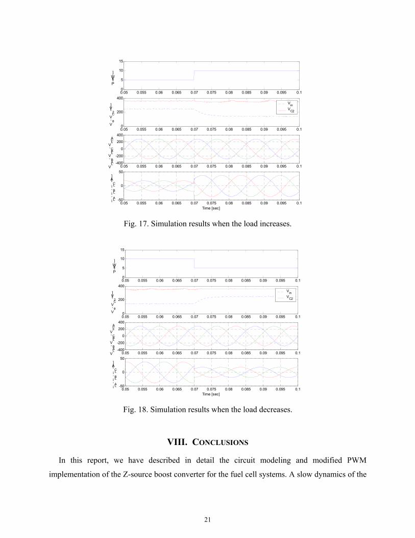
Fig. 14 shows PWM signals of six power switches and the shoot-through that both power

switches in a leg are simultaneously turned on is definitely shown. Fig. 15 and 16 show the

simulation waveforms in steady state without considering the slow dynamics of the fuel cell. Fig.

17 and 18 show the simulation results under the load increase and decrease, respectively. In Fig.

17 and 18, each figure indicates: (a) Power request at 70 msec., (b) Output voltage of the fuel

cell (Vin) and capacitor (VC2), (c) Load line to line voltages (VLAB, VLBC, VLCA), and (d) Load

phase currents (iLA, iLB, iLC). As shown in Fig. 17 and 18 (b), (d), a good voltage regulation of

capacitor voltage (VC2) is presented in spite of a slow change of the fuel cell output voltage and a

load change.

20

0.05 0.055 0.06 0.065 0.07 0.075 0.08 0.085 0.09 0.095 0.10

5

10

15

P [k

W]

0.05 0.055 0.06 0.065 0.07 0.075 0.08 0.085 0.09 0.095 0.10

200

400

Vin

, VC2

[V] Vin

VC2

0.05 0.055 0.06 0.065 0.07 0.075 0.08 0.085 0.09 0.095 0.1-400

-200

0

200

400

VLAB

, VLBC

, VLCA

0.05 0.055 0.06 0.065 0.07 0.075 0.08 0.085 0.09 0.095 0.1-50

0

50

Time [sec]

i LA, i

LB, i

LC [A]

Fig. 17. Simulation results when the load increases.

0.05 0.055 0.06 0.065 0.07 0.075 0.08 0.085 0.09 0.095 0.10

5

10

15

P [k

W]

0.05 0.055 0.06 0.065 0.07 0.075 0.08 0.085 0.09 0.095 0.10

200

400

Vin

, VC2

[V] Vin

VC2

0.05 0.055 0.06 0.065 0.07 0.075 0.08 0.085 0.09 0.095 0.1-400

-200

0

200

400

VLAB, VLBC, VLCA

0.05 0.055 0.06 0.065 0.07 0.075 0.08 0.085 0.09 0.095 0.1-50

0

50

Time [sec]

i LA, i

LB, i

LC [A]

Fig. 18. Simulation results when the load decreases.

VIII. CONCLUSIONS

In this report, we have described in detail the circuit modeling and modified PWM

implementation of the Z-source boost converter for the fuel cell systems. A slow dynamics of the

21

fuel cells and a voltage-current characteristic of a cell are also considered for more realistic

applications. To verify the analyzed circuit model and modified SVPWM method, various

simulation results for two load conditions have been presented from Fig. 14 to Fig. 18 for a

system that needs a 3-phase AC 208 V (L-L)/60 Hz/10 kVA.

ACKNOWLEDGMENT

This work is supported in part by the National Science Foundation under the grant

ECS0105320.

22

REFERENCES

[1] M. N. Marwali and A. Keyhani, “Control of Distributed Generation Systems, Part I:

Voltages and Currents Control,” IEEE Transaction on Power Electronics, 2004. (In Print)

[2] M. N. Marwali, J. W. Jung, and A. Keyhani, “Control of Distributed Generation Systems,

Part II: Load Sharing Control,” IEEE Transaction on Power Electronics, 2004. (In Print)

[3] A. A. Chowdhury, S. K. Agarwal, D. O. Koval, “Reliability modeling of distributed

generation in conventional distribution systems planning and analysis,” IEEE Transactions

on Industry Applications, vol. 39, pp. 1493-1498, Sept.-Oct. 2003.

[4] Y. Zhu and K. Tomsovic, “Adaptive power flow method for distribution systems with

dispersed generation,” IEEE Transactions on Power Delivery, vol. 17, pp. 822-827, July

2002.

[5] J. L. Del Monaco, “The Role of Distributed Generation in the Critical Electric Power

Infrastructure,” IEEE-Power Engineering Society Winter Meeting, vol. 1, pp. 144 –145,

2001.

[6] L. Philipson, “Distributed and Dispersed Generation: Addressing the Spectrum of Consumer

Needs,” IEEE-Power Engineering Society Summer Meeting, vol. 3, pp. 1663 –1665, 2000.

[7] J. Gutierrez-Vera, “Use of Renewable Sources of Energy in Mexico,” IEEE Trans. Energy

Conversion, vol. 9, pp. 442 –450, Sept. 1994.

[8] L.Y. Chiu and B. M. Diong, “An improved small-signal model of the dynamic behavior of

PEM fuel cells,” IEEE 38th IAS Annual Meeting, vol. 2, pp. 709-715, Oct. 2003.

[9] S. Yerramalla, A. Davari, A. Feliachi, “Dynamic modeling and analysis of polymer

electrolyte fuel cell,” IEEE Power Engineering Society Summer Meeting, vol. 1, pp. 82-86,

July 2002.

[10] J. T. Pukrushpan, A. G. Stefanopoulou, and H. Peng, “Modeling and control for PEM fuel

cell stack system,” American Control Conference, vol. 4, pp. 3117-3122, May 2002.

[11] C. J. Hatziadoniu, A. A. Lobo, F. Pourboghrat, and M. Daneshdoost, “A simplified dynamic

model of grid-connected fuel-cell generators,” IEEE Transactions on Power Delivery, vol.

17, pp. 467-473, April 2002.

23

[12] J. T. Pukrushpan, H. Peng, and A. G. Stefanopoulou, “Simulation and analysis of transient

fuel cell system performance based on a dynamic reactant flow model,” Proceedings of

ASME IMECE’02, 2002.

[13] M. D. Lukas, K. Y. Lee, and H. Ghezel-Ayagh, “An explicit dynamic model for direct

reforming carbonate fuel cell stack,”

IEEE Trans. Energy Conversion, vol. 16, pp. 289-295, Sept. 2001.

[14] D. J. Hall and R. G. Colclaser, “Transient modeling and simulation of a tubular solid oxide

fuel cell,” IEEE Transactions on Energy Conversion, vol. 14, pp. 749–753Sept. 1999.

[15] M. D. Lukas, K. Y. Lee, and H. Ghezel-Ayagh, “Development of a stack simulation model

for control study on direct reforming molten carbonate fuel cell power plant,” IEEE

Transactions on Energy Conversion, vol. 14, pp. 1651-1657, Dec. 1999.

[16] Yoon-Ho Kim and Sang-Sun Kim, “An electrical modeling and fuzzy logic control of a fuel

cell generation system,” IEEE Transactions on Energy Conversion, vol. 14, no. 2, pp. 239-

244, June 1999.

[17] K. H. Hauer, “Dynamic interaction between the electric drive train and fuel cell system for

the case of an indirect methanol fuel cell vehicle,”35th IECEC Meeting, vol. 2 , pp. 1317-

1325, July 2000.

[18] G. K. Andersen, C. Klumpner, S. B. Kjaer, and F. Blaabjerg, “A new green power inverter

for fuel cells,” IEEE PESC’02, vol. 2, pp. 727-733, June 2002.

[19] R. Gopinath, Sangsun Kim, Jae-Hong Hahn, M. Webster, J. Burghardt, S. Campbell, D.

Becker, P. Enjeti, M. Yeary, and J. Howze, “Development of a low cost fuel cell inverter

system with DSP control,” IEEE PESC’02, vol. 1, pp. 309-314, June 2002.

[20] A. M. Tuckey and J. N. Krase, “A low-cost inverter for domestic fuel cell

applications,”IEEE PESC’02, vol. 1, pp. 339-346, June 2002.

[21] E. Santi, D. Franzoni, A. Monti, D. Patterson, F. Ponci, and N. Barry, “A fuel cell based

domestic uninterruptible power supply,” IEEE APEC’02, vol.1, pp. 605-613, March 2002.

[22] Fang Zheng Peng, “Z-source inverter,” IEEE Transactions on Industry Applications, vol.

39, no. 2, pp. 504-510, Mar/Apr. 2003.

[23] Jin-Woo Jung and Ali Keyhani, “Design of Z-source Converter for Fuel Cells,” Electric

Supply Industry in Transition, AIT Thailand, 2004.

24

Appendix

A. Matlab Code for the initialization before the Simulink simulation

(Matlab version 6.1: filename: Z_source_PI.m)

% Written by Jin-Woo Jung, 04/03/2004

clear all;

%%%%%%%%%%%%%%%%%%%%%%%%%%%%%%%%%%

% Initialize the plant model parameters %%

%%%%%%%%%%%%%%%%%%%%%%%%%%%%%%%%%%

% fundamental output frequency

f=60; % Hz

w=2*pi*f; % rad/s

% Power rating and limit of fuel cell output voltage

P= 10e3; % Power rating

Vin_min= 150; % minimum voltage of fuel cell output

Vin_max= 360; % maximum voltage of fuel cell output

% Sampling time

Tz=1/60/90; % PWM frequency = 5.4 kHz

% Desired average DC-link voltage (VC2)

Vdc=360; % desired capacitor voltage

% Z-source impedance

L= 200e-6; % L-C impedance

C= 1000e-06; % L-C impedance

25

% Circuit parameters of L-C output filter

Lf= 580e-6; % Inductor

Cf= 380e-6; % Capacitor

Ilimit=3*10e3/120*sqrt(2); % 300% inverter current limit

%Shoot-through period

T0_min= 0; % Vin= 360 V

T0_max = 0.3684; % Vin= 150 V

% Voltage limit for SVPWM

Vmax_DSMC=Vdc*2/sqrt(3); % Line to line voltage limit

Vmax=Vdc*2/3; % Phase voltage limit

% Set desired output voltage (reference voltage)

VLLp= 120*sqrt(6); % line to line peak value (208 RMS)

% Convert abc to qd0 (stationary reference frame)

sr3_2=sqrt(3)/2;

Ks=[1 -0.5 -0.5; 0 sr3_2 -sr3_2; 0.5 0.5 0.5]*2/3;

Ksqd=Ks(1:2, :); % ignore 0 axis

Ksqd3=[Ksqd zeros(2,3) zeros(2,3)

zeros(2,3) Ksqd zeros(2,3)

zeros(2,3) zeros(2,3) Ksqd]; % Transformation matrix

%%%%%%%%%%%%%%%%%%%%%%%%%%%%%%%%%%

% Three PI controller gains %%

%%%%%%%%%%%%%%%%%%%%%%%%%%%%%%%%%%

% PI voltage controller

kp_v= 10; % P gain

ki_v= 0.1; % I gain

26

% PI current controller

kp_i= 1.5; % P gain

ki_i= 0.1; % I gain

% PI DC-link voltage controller

kp= 0.01; % P gain

ki= 0.1; % I gain

upper= 1.15; % Upper limit for saturation

lower_0= 0.8; % Lower limit for saturation

lower_1= 0; % Lower limit for saturation

% Program End

27

B. The Simulink model used in the simulation

(Matlab version 6.1: filename: Z_Source_Inv_PI.mdl)

B-1 Model of Total System Configuration

28

B-2 Model of Fuel Cell

B-3 Model of Power Request

29

B-4 Model of L-C Output Filter

B-5 Model of PWM Inverter Controller

30

B-5-1 Model of PI Voltage Controller

B-5-2 Model of PI Current Controller

B-5-3 Model of PI DC-link Voltage Controller

31

B-5-4 Model of abc to qd Transformation

B-5-5 Model of SVPWM Implementation

B-5-5-1 Model of Vref and angle

32

B-5-5-2 Model of Space Vector Inverter

33

B-5-5-2-1 Model of Sector 1-6 (Upper)

34

B-5-5-2-2 Model of Sector 1-6 (Lower)

35

B-5-5-2-3 Model of V1 – V6 (Upper or lower)

B-6 Model of Load

36