Embed Size (px)
Citation preview

Modeling and Control of Static and Dynamic
Systems with Bayesian NetworksLogos Verlag Berlin 2004
Submitted to the
Technische Fakultat der
Universitat Erlangen–Nurnberg
in partial fulfillment of the requirements for
the degree of
DOKTOR–INGENIEUR
from
Rainer Deventer
Erlangen — 2004

As dissertation accepted from the
Technische Fakultat der
Universitat Erlangen–Nurnberg
Date of submission: 27.10.2003
Date of graduation: 13.1.2004
Dean: Prof. Dr. rer. nat. A. Winnacker
Reviewer: Prof. Dr.-Ing. H. Niemann
Prof. Dr.-Ing. W. Schweiger

Acknowledgments
This thesis was written during my employment at the chair forpattern recognition as a member
of the special research center 396 ’Robust, shortened process sequences for lightweight sheet
parts’. I would like to thank everyone who contributed to thesuccess of this thesis.
Particularly I would like to thank Prof. Niemann for stimulating discussions and for his con-
structive criticism. I also wish to express my gratitude to Prof. Schweiger who acts as second
reviewer. Both reviewers supported me very much by writing quickly their reviews. Further-
more I would like to thank Prof. Ehrenstein and Prof. Geiger for the good cooperation within the
special research center.
Also the good working atmosphere at the institute for pattern recognition was very helpful.
Prof. Denzler provided me with helpful comments and looked carefully through the manuscript.
Additionally he volunteered to write the preface for this thesis. Mr. Popp, the technician at the
institute, assisted me in all questions concerning the hardware.
Additionally I am indebted to my friends and colleagues Mr. Martino Celeghini, Prof.
Joachim Denzler, Mr. Luis Fernandez Dıaz, Dr. Dorthe Fischer, Dr. Oliver Kreis, and Ms.
Alexandra Weichlein for carefully reading my thesis.
Finally I have to thank my parents who supported me during my complete development. I
severely regret that it was not granted to my mother to see me finishing my doctorate.


Contents
Preface v
1 Introduction 1
1.1 Problem presentation . . . . . . . . . . . . . . . . . . . . . . . . . . . . .. . . 1
1.2 State of the art in modeling and control . . . . . . . . . . . . . . .. . . . . . . . 3
1.3 Bayesian networks and their application . . . . . . . . . . . . .. . . . . . . . . 6
1.4 Contribution of the thesis . . . . . . . . . . . . . . . . . . . . . . . . .. . . . . 8
1.5 Overview . . . . . . . . . . . . . . . . . . . . . . . . . . . . . . . . . . . . . . 10
2 An introduction to Bayesian networks 13
2.1 Preliminaries . . . . . . . . . . . . . . . . . . . . . . . . . . . . . . . . . . .. 13
2.2 Definition of Bayesian networks with discrete variables. . . . . . . . . . . . . . 15
2.2.1 Junction tree algorithm . . . . . . . . . . . . . . . . . . . . . . . . .. . 18
2.2.2 Learning algorithms for Bayesian networks . . . . . . . . .. . . . . . . 25
2.3 Hybrid Bayesian networks . . . . . . . . . . . . . . . . . . . . . . . . . .. . . 29
2.3.1 Definition of hybrid Bayesian networks . . . . . . . . . . . . .. . . . . 30
2.3.2 Inference in hybrid Bayesian networks . . . . . . . . . . . . .. . . . . . 33
2.3.3 Learning the parameters of a hybrid Bayesian network .. . . . . . . . . 39
2.4 Dynamic Bayesian networks . . . . . . . . . . . . . . . . . . . . . . . . .. . . 42
3 Control of dynamic systems 45
3.1 Description of linear dynamic systems . . . . . . . . . . . . . . .. . . . . . . . 46
3.1.1 Normal forms . . . . . . . . . . . . . . . . . . . . . . . . . . . . . . . . 51
3.1.2 Kalman filter . . . . . . . . . . . . . . . . . . . . . . . . . . . . . . . . 52
3.1.3 Description of dynamic systems by difference equation . . . . . . . . . . 55
3.2 Non-Linearities in dynamic systems . . . . . . . . . . . . . . . . .. . . . . . . 57
3.3 Controlled systems . . . . . . . . . . . . . . . . . . . . . . . . . . . . . . .. . 61
i

ii CONTENTS
3.3.1 Different types of controllers . . . . . . . . . . . . . . . . . . .. . . . . 63
4 Modeling Linear Dynamic Systems 69
4.1 Principle of a model based controller . . . . . . . . . . . . . . . .. . . . . . . . 70
4.1.1 Calculation of the input signal . . . . . . . . . . . . . . . . . . .. . . . 75
4.1.2 Evaluation of the controller . . . . . . . . . . . . . . . . . . . . .. . . 76
4.2 Trained Bayesian controller . . . . . . . . . . . . . . . . . . . . . . .. . . . . . 78
4.3 Higher order Markov-model . . . . . . . . . . . . . . . . . . . . . . . . .. . . 83
4.4 Modeling of higher order systems . . . . . . . . . . . . . . . . . . . .. . . . . 88
4.5 Comparison to PI and Dead-Beat controller . . . . . . . . . . . .. . . . . . . . 90
5 Bayesian networks for modeling nonlinear dynamic systems 97
5.1 Prototypical modeling of nonlinear units . . . . . . . . . . . .. . . . . . . . . . 97
5.2 Control of non-linear systems . . . . . . . . . . . . . . . . . . . . . .. . . . . . 106
5.2.1 Expansion of difference equation model . . . . . . . . . . . .. . . . . . 107
5.2.2 State-space model . . . . . . . . . . . . . . . . . . . . . . . . . . . . . 111
6 Modeled manufacturing processes 115
6.1 Hydroforming . . . . . . . . . . . . . . . . . . . . . . . . . . . . . . . . . . . .115
6.1.1 Preforming and calibration . . . . . . . . . . . . . . . . . . . . . .. . . 115
6.1.2 Modeling the forces of the press . . . . . . . . . . . . . . . . . . .. . . 118
6.1.3 Laser beam welding . . . . . . . . . . . . . . . . . . . . . . . . . . . . 119
6.2 Injection moulding . . . . . . . . . . . . . . . . . . . . . . . . . . . . . . .. . 122
7 Process models 127
7.1 Hydroforming . . . . . . . . . . . . . . . . . . . . . . . . . . . . . . . . . . . .128
7.1.1 Preforming and calibration . . . . . . . . . . . . . . . . . . . . . .. . . 128
7.1.2 Modeling the forces of the press . . . . . . . . . . . . . . . . . . .. . . 133
7.1.3 Laser beam welding . . . . . . . . . . . . . . . . . . . . . . . . . . . . 137
7.2 Injection moulding . . . . . . . . . . . . . . . . . . . . . . . . . . . . . . .. . 145
7.2.1 Results . . . . . . . . . . . . . . . . . . . . . . . . . . . . . . . . . . . 146
7.2.2 Test plan for injection moulding . . . . . . . . . . . . . . . . . .. . . . 149
8 Real-time 151
8.1 Number of time-slices . . . . . . . . . . . . . . . . . . . . . . . . . . . . .. . . 152
8.1.1 Dependency on the number of nodes used for the future . .. . . . . . . 152

CONTENTS iii
8.1.2 Dependency on the number of nodes used for the past . . . .. . . . . . 156
8.2 Stable Inference algorithm . . . . . . . . . . . . . . . . . . . . . . . .. . . . . 158
9 Outlook and Summary 161
9.1 Outlook . . . . . . . . . . . . . . . . . . . . . . . . . . . . . . . . . . . . . . . 161
9.1.1 Usage of Bayesian networks as a controller . . . . . . . . . .. . . . . . 161
9.1.2 Modeling manufacturing processes . . . . . . . . . . . . . . . .. . . . 165
9.2 Summary . . . . . . . . . . . . . . . . . . . . . . . . . . . . . . . . . . . . . . 166
Bibliography 171
Appendix 181
Index 186

iv CONTENTS

Preface
Todays modern manufacturing processes face shorter production cycles, demand for more flex-
ibility and higher quality of the products. This results in an increased need for new methods
in the area of modeling and controlling of process chains, that allows self-adaption as well as
integration of expert knowledge.
This is the focus of the book at hand. It is one of the first booksthat merges techniques
from classical control theory and modern, probabilistically motivated artificial intelligence to
develop new methods for modeling and adaptive control of dynamic processes. The key element
is a Bayesian network, that allows the explicit modeling of dependencies between events. Thus,
expert knowledge can be easily integrated. However, in thisframework also automatic detection
of the dependencies is possible. This makes Bayesian networks perfectly suited for modeling
and control of manufacturing processes: during the first design expert knowledge can be used,
while in service the parameter can be adapted online withoutuser intervention.
The book gives a comprehensive introduction to Bayesian models as well as to control the-
ory. A link is made between classical methods for describingand handling linear and non-linear
dynamic systems at the one side and dynamic Bayesian networks on the other side. Although the
book describes two applications from manufacturing technology to prove the applicability, the
theory is developed in a general way. First, the reader clearly gets used to linear and non-linear
dynamic systems before the relation is shown to dynamic Bayesian networks. Well known non-
linear units, like saturation or hysteresis, are discussedin the following. The results of modeling
hydroforming and injection moulding show the benefits of theapproach.
Prof. Joachim Denzler
v

vi PREFACE

Chapter 1
Introduction
1.1 Problem presentation
Manufacturing technology has to face several challenges. The time to market is getting shorter
[sfb95; GL99] on the one side, but a high quality is of great importance, as an unsatisfied cos-
tumer might change to the competitor [Pfe93] and tell his opinion a lot of other people [Pfe93].
An additional problem for countries like Germany are high wages [sfb95], so that there is a high
need for automation. The collaborative research center SFB396 tries to master this challenge by
several measures, e.g. by experiments with new materials orcombination of new materials, or
the integration of several process-steps. To achieve the goals also modeling plays an important
role [sfb95]. This is not only valid in the scope of the collaborative research center, but also for
manufacturing technology in general [Lan96].
A model is a simplified image of reality which abstracts, depending on the intended appli-
cation, from unimportant details. In [Lan96] three different groups of models are distinguished.
Process modelsare a quantitative mapping of continuous processes. A second group arecontrol
models, describing the relationship between control devices and the technical processes.Infor-
mation technical modelsare used, if automation with a process computer is intended,and they
represent the automation tasks.
Within the scope of this thesis only process models are discussed. Process models can fur-
ther be characterized as either static, e.g. used for the calculation of suitable settings for input
variables, or dynamic, if the course of the measured variables is of interest. An example for a
static process model is the modeling of the distribution of the forces during hydroforming, with
the aim to guarantee an equal distribution at all points of measurement.
Depending on the planned application, different means for modeling are used, e.g. mathe-
1

2 CHAPTER 1. INTRODUCTION
matical models or Petri nets [Lan96].
In automation also statistical methods are used, e.g. control charts [Pfe98; GL99]. Control
charts record the output variables, representing the quality of the process. Additionally upper
and lower thresholds are defined. When measurements are beyond those thresholds an action is
required. In this thesis also a statistical approach is suggested, based on Bayesian networks. But
in contrast to control charts the suggested approach aims atautomatic control, the input variables
are directly calculated using the statistical model.
Bayesian networks represent the distribution of multiple,discrete or continuous, random
variables. For a better overview, the variables are displayed in an acyclic, directed graph. The
broad applicability of Bayesian networks can be attributedto several advantageous features.
• There are a lot of training algorithms available, both for the structure and the parameter of
Bayesian networks [Bun94; Jor99; Mur02; RS97; GH94; FK03].
• Efficient inference algorithms are developed in the last 15years [LS88; Lau92; LSK01;
Pea88].
• It is possible to work with missing measurements and hiddenvariables [Mur98b].
To apply Bayesian networks to automation, there are a numberof requirements, listed shortly
in the following paragraphs. Of course, most of these requirements are not only specific for
Bayesian networks, but for modeling in general.
First, the accuracy of the model is required; i.e., the deviation between reality and the predic-
tions of the models should be minimized.
The second desired feature is the ability to generalization. That means the model must be
able to make predictions also for yet unpresented settings of the in- or output variables.
In many cases the structure of the model is also subject of modeling [Lan96]. In dependency
on the required application other demands may occur.
Sometimes a number of experiments is executed, to find out a suitable setting for the input
variables. To reduce costs, usually test-plans are used. The aim is to reduce the number of
experiments with a small impact on the knowledge gained by the experiments. This leads to a
low number of training sets which complicates a statisticalanalysis, particularly with discrete
Bayesian networks.
If the model is to be applied in quality management, there is aneed for a permanent adaptation
as additional data are collected during the production process.
When dynamic models are applied in control, other requirements have to be met.

1.2. STATE OF THE ART IN MODELING AND CONTROL 3
• As a controller should act without supervision of an operator, a robust model and controller
is needed. An oscillation has to be avoided in all cases.
• The calculation of the manipulated variables has to be donein real-time. The required
response-time depends on the controlled system.
• Failure of sensors should be compensated, so that stability of control is not affected.
• An on-line adaptation of model-parameters is desirable, to keep track with a changing
environment.
In the next two sections the state of the art in control theoryis discussed, and a brief overview
about applications of Bayesian networks is given. In section 1.4 the contribution of this thesis to
the field of modeling and control is sketched.
1.2 State of the art in modeling and control
In section 1.1 it is mentioned, that intelligent modeling and control plays an important role for
manufacturing processes and industrial production. As thelargest part of this thesis considers
this problem from the point of view of Bayesian networks, this section deals with alternative
approaches, so that a more comprehensive picture is given. The approaches of traditional control
are omitted, they are discussed in chapter 3.
In the following different approaches from artificial intelligence are discussed mainly from
the point of view of modeling manufacturing processes and ofindustrial control. In the last
decades rule-based systems, neural networks, fuzzy control, evolutionary systems, and statistical
process control are frequently applied approaches in automatic process control [JdS99; FJdS99].
Rule-based systemsuse a knowledge base, with several rules, to define suitable control ac-
tions. In comparison to the other algorithms, they play a smaller role in industrial control. Major
problems are the knowledge acquisition, needed to develop the knowledge base. An additional
drawback is, that usually a set of rules is not suited to generate numerical control signals, needed
for control purposes. One of the advantages is, that it is easy to generate an explanation for the
suggested control action.
Neural networksare typically divided into an input layer, several hidden layers, and an output
layer. Typically each node in a layer is connected to each node in the succeeding layer. Of course
there are several exceptions, like Boltzmann machines [Dev94] and Hopfield nets [RM86], which
are fully connected. Each layer consists of several nodes. The behavior of the complete net is

4 CHAPTER 1. INTRODUCTION
governed by the weights of the connections between the nodesand the activation function, which
maps the weighted input of the parent nodes to the output. During the training process, the
weights of a neural network are adapted, while the type of nodes, the structure, and the activation
function are kept constant. For the training process two different scenarios are distinguished,
supervised and unsupervised learning.
During the unsupervised learning process only the input is given. It is the task of the training
process, to detect frequently occurring patterns. One of the most popular representative is the
Kohonen network, which consists of one in- and output layer. During the training process the
weights of the winner-neuron, whose weights are closest to the input, are adapted, so that its
weights get closer to the presented input. Additionally, the weights of its neighbors are changed
in the same way, depending on the distance to the winner neuron. At the end of the training
process neighbored neurons react on similar inputs.
In supervised learning the input and the desired output are presented to the net. A well-
known example is the backpropagation algorithm. In this case the weights are adapted in order
to minimize the error between actual and required output.
For the purpose of control one should keep in mind that usually the direction of inference
is fixed. Thus it is impossible to train a neural network, so that it simulates the behavior of a
dynamic system and put the desired value at the output nodes to get the manipulated value. In
[WSdS99] different methods for neural control are discussed.
The simplest one issupervised control. Here the neural network is trained, so that it copies
the behavior of an existing controller. After the training is finished the neural network is used
instead of the controller, used for the training.
In the approach of ”direct inverse control” the network “is trained to learn the inverse dy-
namics of the system” [WSdS99]. That means that the systems output is used as the input of the
neural network, which tries to predict the system’s input which has led to the observed output.
To correct the weights the predicted input is compared with the actual one, so that supervised
learning is possible. After the training process the neuralnetwork acts as controller; i.e., the
desired value is used as input of the neural network, the output of the net is used as input signal
for the dynamic system.
In ”neural adaptive control” the neural network is trained to learn the parameters of a plant
and adapt a controller based on this information. In contrast to supervised control and to direct
inverse control the neural network does not act as controller, but to improve the performance of
an existing controller [WSdS99]. When only information about success or failure are available
reinforcement learning could be used.

1.2. STATE OF THE ART IN MODELING AND CONTROL 5
The great advantage of neural networks is the ability to copealso with new situations and to
learn nonlinear functions with an arbitrary precision. A drawback is that a neural network is a
kind of black box, so that there is nearly no possibility to interpret the training results.
Another approach is Fuzzy Logic, based on the theory of Fuzzysets, suggested by Lotfi
Zadeh in the late sixties [Zad65]. In principleFuzzy Control[Pre92; HR91] is based on a number
of control rules like
If ’Pressure’ = ’high’ and ’Temperature’ = ’high’ then ’Cooling temperature’ = ’low’,
which are given either by a knowledge engineer or are trainedin combination with a neural net-
work. In comparison to a rule based system, the predicates ofthe preconditions are not evaluated
in a boolean manner, but are mapped to an interval [0 1], representing the degree, a precondition
is fulfilled. After the degree of truth is assigned to each predicate, the boolean operators are ap-
plied. Typically the result of the ’and’-operator is mappedto the minimum of both truth-degrees,
the ’or’-operator is mapped to the maximum of both operands.In this way a degree of truth is
assigned to the conclusion. To combine the results of several rules, making predictions for the
same variable,defuzzyficationhas to be applied to all results. A method regularly applied,is to
use the center of gravity as final result. Fuzzy control can becombined with neural networks to
train the fuzzy rules or with a rule based system to enable it to generate numerical solutions.
When control is regarded as an optimization problemevolutionary algorithmscan be applied
[Nom99]. An example might be the assignment of jobs to different manufacturing systems. The
main idea of evolutionary algorithms is to code the solution, e.g. the algorithm used for control,
in so called chromosomes, e.g. as strings or as trees with operators and variables as leaves and
nodes. At the beginning a lot of solutions are collected in aninitial population. Afterwards
the quality of the solution is judged by a fitness function. Togenerate a new population, new
chromosomes are generated using the old population, where chromosomes, representing a good
solution are used more frequently. The new chromosomes are changed with a low probability,
e.g. by flipping a bit in the chromosomes. This imitates the process of mutation. After the new
population is generated, the iteration of evaluation and generation of new chromosomes begins
once again. The idea is that the overall quality of the solutions increases, as better chromosomes
are preferred during reproduction. A monotonous increase of the quality can be guaranteed, when
the best chromosome is kept in the population, i.e. the elitist strategy is applied. Evolutionary
algorithms are applied, when the fitness function can not be differentiated, i.e. the application of
gradient descent is impossible.
Statistical methodsare seldom used. Chapter 7 of [Lu96] discusses the application of statisti-
cal process control, based on statistical process charts. The idea is to apply principal component

6 CHAPTER 1. INTRODUCTION
analysis on both the domain of in- and output variables, to reduce the dimension, and afterwards
learn the dependency between in- and output variables. Thusa prediction of the quality of the
output is possible, and it is possible to trigger the change of the input variables in real time, when
the process is out of control.
This section shows, that there are a lot of possibilities forintelligent process control, Bayesian
networks are usually not mentioned in the literature about industrial control. The next section
will give a coarse overview about the application of Bayesian networks to show, that in principle
the preconditions for the application of Bayesian networksin control are given.
1.3 Bayesian networks and their application
In the last section it was discussed that there are already a lot of means to deal with control
problems. This section shows that Bayesian networks are applied in different domains, e.g.
medical diagnosis, user-modeling, and data-mining. Some applications are time critical [HB95;
HRSB92]. As a lot of training algorithms are available the most important prerequisites for
self-adaptive control are given.
In general Bayesian networks can be regarded as a mean to represent the relation between
several random variables in a directed graph. The nodes in that graph represent the random
variables. The arcs between the nodes stand for the dependency of the nodes.
When a distribution of discrete random variables has to be modeled, the effort grows expo-
nentially with the number of used nodes. This has led to the conclusion, that it is an intractable
task to develop an expert system, based on probability theory [Jen96]. To avoid this exponential
growth of complexity, the inference process in a Bayesian network is based on local distributions
of one random variable, depending on its parents. This measurement makes the statistical in-
ference tractable and reduces also the number of parameters. In a decision theoretic framework
influence diagrams [Zha98a; Zha98b; Jen01], i.e. Bayesian networks with additional nodes to
represent actions and their utility, are used. When time dependent relations have to be repre-
sented dynamic Bayesian networks can be used. A deeper introduction in Bayesian network and
dynamic Bayesian network is given in chapter 2.
The most popular application of Bayesian networks seems to be the Office-Assistant, de-
livered the first time as part of the Office 97 package. The assistant was developed within the
framework of the Lumiere project [HJBHR98; HH98], starting 1993. The aim of the project
was to find out the goal and the needs of the user, based on the state of the program, past ac-
tions, and on a possible query to the help system. In a prototype it was even tried to save the

1.3. BAYESIAN NETWORKS AND THEIR APPLICATION 7
estimated competency of the user in the registry, which should be used as an additional source
of information. As the aims of the user vary within time, a Dynamic Bayesian network is used
for the representation of the user’s goal [HJBHR98; Had99].The past actions are transformed
by the Lumiere Events Language into predicates, which can be regarded as random variables
and modeled in a Bayesian network. Thus the program can identify pattern like plan-less search
and a pause which might indicate the need for help. Using a Bayesian network a probability
distribution of the user’s need is calculated. In a prototype a icon popped up, when a threshold is
exceeded. In the final version this knowledge is used to improve answering queries to the system
by the identification of the user’s goal.
From the historical view the first real-world applications are medical expert systems, e.g. the
MUNIN system [Kit02; AJA+89] for “electromyographic diagnosis of the muscle and nerve
system”[Lau01], the pathfinder system [HHN91] for “diagnosis of lymph vertex pathology”
[Lau01], which was later commercialized as the Intellipathsystem [Jen96]. Additional exam-
ples are the probabilistic reformulation [SMH+91] of the INTERNIST-1/QMR knowledge base
and the Child system at the Great Ormond Street Hospital in London for the diagnosis of heart
diseases [Jen96].
The MUNIN system, developed at the University of Aalborg, isused for the diagnosis of 22
different diseases [Kit02] with 186 symptoms, and has the ability to detect several diseases at
the same time. It is structured in 12 units, representing different muscles and nerves, with 20 -
150 nodes each. Each unit is structured in three layers, where the first two layers represent the
pathological variables, and the last layer the variables for diagnosis.
In comparison to the MUNIN system, the PATHFINDER system hasa simpler structure.
There is one central variable with more than 60 states, representing the different diagnoses. Thus
the system is not able to represent more than one disease at the same time. As parents of the
diagnosis variable there are 130 information variables, sometimes linked with each other [Jen96].
First attempts of user modeling are also found in the PATHFINDER system [HJBHR98] in order
to adapt the questions and answers of the expert system to thecompetence of the user.
The Child system helps the pathologists at the hotline of theGreat Ormond Street Hospital,
to decide whether a blue baby should be transported to a special hospital or not. The structure
and probabilities was initialized by experts, and later refined by existing cases. As a result the
system could compete with experts in that domain [Jen96].
Another domain of application is the modeling of technical systems. A system, based on a
Bayesian model of a technical process is the Vista system [HB95; HRSB92], “which has been
used for several years at NASA Mission Control Center in Houston” [Had99]. Its aim is to

8 CHAPTER 1. INTRODUCTION
decide in real-time which information is displayed to the operators in the control center. To do so
a model of the propulsion system, the example used by the Vista-project, is developed including
all types of possible errors, e.g. failure of sensor data. When the Bayesian model detects an
abnormal situation, the most probable causes are displayedto the user together with the necessary
sensor data, to deal with the situation. The utility of the information is measured by the expected
value of revealed information, a measure used to judge the utility of new information. The
decision, which information is displayed to the user, is based on an influence diagram, where the
utility of each action is measured be the expected value of this information.
The intended application in this thesis has to react in real-time. Examples for systems reacting
in real-time are of course the Vista system. Another exampleis object detection and tracking in
images of an infrared camera, supported by Bayesian networks[Pan98]. Also in control Bayesian
networks are discussed. Welch [WS99] discusses sorting of contaminated waste with a hybrid
Bayesian network. To achieve real-time properties only parts with changed evidence are updated.
This section has only shown the most prominent examples, other applications are Data-
Mining [Hec97], trouble-shooting, e.g. for printer [BH96;SJK00], and surveillance of an un-
manned underwater vehicle [Had99]. A rich source of additional applications is found in [CAC95;
HMW95; Kit02; Lau01; Had99]. Haddawy [Had99] and F. V. Jensen [Jen01] offer a list of avail-
able toolboxes for modeling Bayesian networks.
1.4 Contribution of the thesis
As seen in section 1.1, static and dynamic process models aredistinguished. Applicable models
are developed in both domains.
Static modelsFor static models, the technique of piecewiselinear approximationis evolved.
The main idea is to represent some input parameters both by a discrete node and a continuous
node. The discrete nodes are used to implement a kind of skeleton of the desired function. The
number of states, being proportional to the number of pointsin the skeleton, depends on the
required accuracy and is restricted by the available training data. This approach has several
advantages.
• From the practical point of view no special software is required.
• The idea is based on the general idea of function approximation by (multiple) Taylor series,
it is not only applicable in the domain of modeling manufacturing processes. It is expected
that this technique is also applicable, e.g. in the field of data-mining.

1.4. CONTRIBUTION OF THE THESIS 9
• Both discrete and continuous nodes are implemented directly. Thus no discretization is
required. Therefore loss of information, caused by discretization, is avoided.
• As shown in section 5.1 each node has a special meaning. Thatis, it is easy to incorporate
a-priori knowledge into the model. For example it is easy to deduce initial parameters for
the Bayesian network. Also the interpretation of the training results is easy, so that the
learned parameters can be used to gain insight in the modeledprocesses.
The concept of modeling a function or a manufacturing process by linear approximation
by multiple Taylor series is applied to different manufacturing processes, e.g. to preforming and
calibration of hydroforming, and to injection moulding. Inall cases a great accuracy of the model
is demonstrated. A comparison with the standard deviation of the different processes shows that
a large part of the prediction error is due to scattering of the data.
Also theability to generalizationof Bayesian models is satisfactorily shown. This is partic-
ularly of importance, because test-plans that lead to missing configurations are frequently used
in manufacturing technology. If the observation of a missing configuration is a prerequisite for
the training of the model generalization fails. The thesis discusses the relationship between test-
plans and the structure of the Bayesian networks. It is suggested that for each set of discrete
nodes, being parent of an arbitrary node, all possible settings of the parent nodes have to be
observed. This criterion is applied with great success to the modeling of laser beam welding.
The development of Bayesian networks for different manufacturing processes shows that
Bayesian networks provide a suitable mean to build accuratemodels, which make sensible pre-
dictions even for yet unpresented inputs.
Dynamic modelsThe second focus of the thesis is the modeling of dynamic, in most of
the cases linear, processes. A framework is developed, to use dynamic Bayesian networks as
controller. The main idea is to estimate the state of the system using information about former
in- and output signals. Using the desired value as additional source of information, the Bayesian
network is able to calculate the required input signals, which lead to the desired output. By
comparison between the predicted and the observed output, the disturbance variable is estimated.
Assuming, that the disturbance value changes slowly in comparison to the sampling period, the
estimation of the disturbance variable is propagated to thefuture and can therefore be included
in the calculation of the input signal.
To ensure abroad applicabilitya general model (state space model), well-known in control
theory, is used as controlled system to test the new approach. This model can easily be trans-
formed into two different structures for the dynamic Bayesian network. First, the state space

10 CHAPTER 1. INTRODUCTION
approach, where the information about the state of the system is stored in hidden state nodes, can
be used directly to deduce the structure.
In the second approach (difference equation model) the information about the state of the
system is gathered by access to former in- and output nodes. Acomparison between the state-
space approach and the difference equation approach shows that the latter is more stable in all
our experiments. The reason is that the lower number of hidden nodes leads to better training
results.
Thus the primary precondition, thestability of a controller is fulfilled. In a second step the
provided accuracy, depending on the number of time-slices and therefore on the time required
for inference, is tested. It turns out, that the number of time-slices can be severely reduced.
Reducing the number of time-slices leads only to a minor reduction of the quality in terms of the
steady state error and the sum of the squared error.
For hybrid dynamic Bayesian networks inference time is proportional toknpast+nfuture with
k as the number of configurations per timeslice andnpast + npast as the number of time-slices
used to represent past and future. Thus this result is of great importance also for hybrid, dynamic
Bayesian networks. Despite the encouraging results inference time remains a great problem
before hybrid Bayesian networks might be applied for control purposes.
1.5 Overview
This thesis is situated at the intersection of different domains. First the thesis can be seen from
the point of view of the intended application, i.e. the modeling of manufacturing processes and
the control of dynamic systems. On the other hand the used algorithms are from the domain
of mathematics or computer science. As it is the aim that thisthesis is understandable for both
engineers and computer-scientists an introduction is given in all domains. Chapter 2 deals with
an introduction to Bayesian networks. A focus of this chapter are hybrid Bayesian networks,
as they are needed to model nonlinear processes. Additionally, the inference process used for
hybrid Bayesian networks, is also used for Dynamic Bayesiannetworks.
Chapter 3 introduces the most important points from controltheory. Major theme is the
state space description, including a short discussion of normal forms. Also the description of
dynamic systems by difference equations is explained, as this theory provides the background of
our models. Additional points are the setting of controllerparameter’s, to provide us with means,
to compare Bayesian controller with traditional ones.
The experiments with dynamic systems are discussed in chapters 4 and 5. The former dis-

1.5. OVERVIEW 11
cusses the application of Bayesian controllers to linear dynamic systems and the comparison of
state space and difference equation model.
The latter discusses the research concerning modeling and control of non-linear systems. The
concept of linear approximation by multiple Taylor series is introduced. In the second part of
chapter 5 the control of nonlinear systems is discussed.
Chapter 6 introduces briefly the modeled manufacturing processes. This chapter provides
only a short discussion of the parameters. The physical background is omitted.
The models developed for the manufacturing processes that are introduced in chapter 6, are
provided in chapter 7. Similar techniques to those, discussed in chapter 5, are used. An additional
requirement, discussed in chapter 8, is real-time. Here themeasures which can be taken to react
in real-time, mainly the dependency on the number of time slices, is examined. The thesis
finishes with an overview about the results and suggestions for future work in chapter 9.

12 CHAPTER 1. INTRODUCTION

Chapter 2
An introduction to Bayesian networks
2.1 Preliminaries
It is our aim to model technical processes using statisticalmeans. This section will shortly
introduce the terminology of probability theory, i.e. random variables and their dependencies are
discussed. A deeper introduction is given in [Bre69; Bre73].
Manufacturing processes depend on many different parameters, e.g. welding depends on the
power and the velocity of the laser beam. The quality of the joint might be measured by the
tensile strength, i.e. the force needed to divide the two blanks. In our experiments a forceF in
an interval [0 N , 5200 N] as set of possible outcomesΩ was measured.
In a first case the engineer might be only interested whether the tensile strength exceeds a
thresholdFmin, i.e. a mapping
F1(ωr) =
1 if ωr ≤ Fmin
2 otherwise(2.1)
from the outcome of an experimentωr to a finite set1 2 is used. In this caseF1 is adiscrete
random variableasF1(ωr) has only a finite number of possible values.
In a second case the tensile strength itself is of importance, i.e. the identity is used as mapping
F2(ωr) = ωr. In this case the domain of the mappingF2 is infinite,F2 is acontinuous random
variable. In the following discrete random variables are denoted byX, continuous ones byY or
Z.
It is possible to assign a probabilityP (X(ωr) = x), abbreviated byP (x), to the resultX(ωr).
For continuous random variables a distributionp(Y (ωr) = y), or shorterp(y), has to be used, as
13

14 CHAPTER 2. AN INTRODUCTION TO BAYESIAN NETWORKS
it is not possible to assign a positive probability to a single eventy.
When modeling technical processes usually more than one random variable is involved, i.e.
dealing with probabilitiesP (X1, X2, · · · , XnN) is essential. Sets of random variablesX =
X1, X2, · · · , XnN are denoted by calligraphic characters, thusP (X1, X2, · · · , XnN
) is abbre-
viated byP (X).
A probability table, which assigns a probability to each event(X1 = x1, X2 = x2, · · · , XnN=
xnN), will grow exponentially with the number of random variablesnN . To factorize the proba-
bility P (X1, X2, · · · , XnN) theconditional probability
P (X1|X2) =P (X1, X2)
P (X2)(2.2)
might be used to rewriteP (X1, X2, · · · , XnN) to
P (X1, X2, · · · , Xn) = P (X1)
nN∏
i=2
P (Xi|Xi−1, · · · , X1) , (2.3)
which is known as thechain rule. SometimesP (X1|X2, X3) = P (X1|X2) holds, that is the
state of the random variablesX3 does not matter, provided that the state ofX2 is known. In
this caseX1 andX3 are calledconditionally independentgivenX2, denoted byX1⊥⊥X3|X2.
WhenX2 is empty,X1 andX3 are calledindependent.
Conditional independency can be used, to rewrite the chain rule to
P (X1, X2, · · · , XnN) = P (X1)
nN∏
i=2
P (Xi|P(Xi)) , (2.4)
whereP(Xi) ⊆ X1, X2, · · · , Xi−1 are called theparentsof Xi. Variables which are not in the
set of parentsP(Xi) are assumed to be conditionally independent ofXi. WhenP(Xi) is a true
subset ofX1, X2, · · · , Xi−1, the conditional probability table forP (Xi|P(Xi)) has less entries
thanP (Xi|X1, X2, · · · , Xi−1).
As an example a snapshot of a family’s life is regarded. First, the seasonS ∈ ’spr’ ,’sum’
, ’fal’,’ win’ which has an influence on the state of the heatingH ∈ ’on’ ,’off ’, and on
problems starting the car (SP ∈ ’yes’ ,’no’), is observed. The heating is only switched on,
when the family is not absent (A ∈ ’yes’ ,’no’. The last random variable is the cost of energy
Ec ∈ ’ low’ ,’medium’ ,’high’. The probability distribution
P (S, A, H, SP, Ec) = P (S)P (A|S)P (H|S, A)P (SP|S, A, H)P (Ec|S, A, H, SP) (2.5)

2.2. DEFINITION OF BAYESIAN NETWORKS WITH DISCRETE VARIABLES 15
P (A)
A =’yes’ 0.15A =’no’ 0.85
Table 2.1: Probabili-ties for nodeAbsent
P (S)
S =’spr’ 0.25S =’sum’ 0.25S =’fal’ 0.25S =’win’ 0.25
Table 2.2: Probabili-ties for nodeSeason
P (Ec|H) H =’on’ H =’off ’
Ec =’ low’ 0.1 0.9Ec =’med’ 0.7 0.05Ec =’high’ 0.2 0.05
Table 2.3: Conditional probabilities for costs ofenergyEc
P (H =’on’ |S, A) A =’yes’ A =’no’
S =’spr’ 0.1 0.3S =’sum’ 0.01 0.05S =’fal’ 0.1 0.3S =’win’ 0.2 0.99
Table 2.4: Conditional probabilities for nodeHeating
P (SP) P (SP =’yes’ |S)
S =’spr’ 0.05S =’sum’ 0.05S =’fal’ 0.05S =’win’ 0.3
Table 2.5: Conditional probabili-ties for node starting problemsSP
might be simplified to
P (S, A, H, SP, Ec) = P (S)P (A)P (H|S, A)P (SP|S)P (Ec|H) (2.6)
which reflects the assumption that, e.g., the probability ofabsence does not depend on the season,
and that the costs of energy are independent from the season and of being absent, provided that
the state of the heating is given.
The probabilities for this example can be defined as in tables2.1 – 2.5. They will be used later
in this chapter to illustrate the inference algorithm for Bayesian networks. Table 2.4 shows only
the probability forP (H =’on’ |S, A). As the probabilities sum to oneP (H =’off ’ |S, A) =
1− P (H =’on’ |S, A). The probabilities forSP =’no’ are calculated similarly.
2.2 Definition of Bayesian networks with discrete variables
To illustrate conditional independency, a directed acyclic graph (DAG) with edges pointing from
the parents ofP(Xi) to Xi is used.
The DAG representing the independencies of equation (2.6) is pictured in figure 2.1. These
considerations result in the definition of aBayesian network. Bayesian networks (BNs) are a
compact graphical representation of a probability distribution, and exhibit the conditional inde-
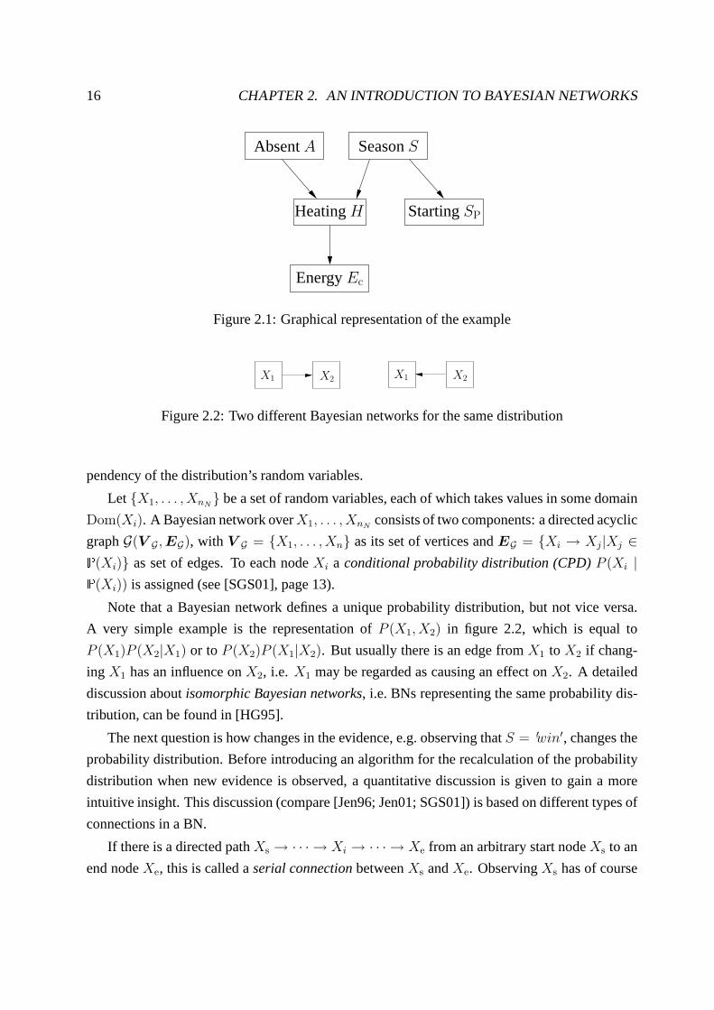
16 CHAPTER 2. AN INTRODUCTION TO BAYESIAN NETWORKS
AbsentA SeasonS
HeatingH StartingSP
EnergyEc
Figure 2.1: Graphical representation of the example
X1X1 X2X2
Figure 2.2: Two different Bayesian networks for the same distribution
pendency of the distribution’s random variables.
Let X1, . . . , XnN be a set of random variables, each of which takes values in some domain
Dom(Xi). A Bayesian network overX1, . . . , XnNconsists of two components: a directed acyclic
graphG(V G, EG), with V G = X1, . . . , Xn as its set of vertices andEG = Xi → Xj|Xj ∈P(Xi) as set of edges. To each nodeXi a conditional probability distribution (CPD)P (Xi |P(Xi)) is assigned (see [SGS01], page 13).
Note that a Bayesian network defines a unique probability distribution, but not vice versa.
A very simple example is the representation ofP (X1, X2) in figure 2.2, which is equal to
P (X1)P (X2|X1) or to P (X2)P (X1|X2). But usually there is an edge fromX1 to X2 if chang-
ing X1 has an influence onX2, i.e. X1 may be regarded as causing an effect onX2. A detailed
discussion aboutisomorphic Bayesian networks, i.e. BNs representing the same probability dis-
tribution, can be found in [HG95].
The next question is how changes in the evidence, e.g. observing thatS = ′win′, changes the
probability distribution. Before introducing an algorithm for the recalculation of the probability
distribution when new evidence is observed, a quantitativediscussion is given to gain a more
intuitive insight. This discussion (compare [Jen96; Jen01; SGS01]) is based on different types of
connections in a BN.
If there is a directed pathXs → · · · → Xi → · · · → Xe from an arbitrary start nodeXs to an
end nodeXe, this is called aserial connectionbetweenXs andXe. ObservingXs has of course
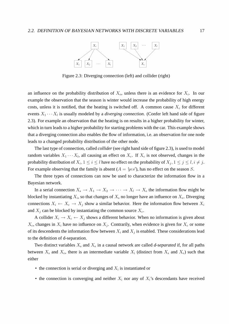
2.2. DEFINITION OF BAYESIAN NETWORKS WITH DISCRETE VARIABLES 17
Xc
Xc
X1
X1
X2
X2 Xl
Xl· · ·
· · ·
Figure 2.3: Diverging connection (left) and collider (right)
an influence on the probability distribution ofXe, unless there is an evidence forXi. In our
example the observation that the season is winter would increase the probability of high energy
costs, unless it is notified, that the heating is switched off. A common causeXc for different
eventsX1 · · ·Xl is usually modeled by adiverging connection. (Confer left hand side of figure
2.3). For example an observation that the heating is on results in a higher probability for winter,
which in turn leads to a higher probability for starting problems with the car. This example shows
that a diverging connection also enables the flow of information, i.e. an observation for one node
leads to a changed probability distribution of the other node.
The last type of connection, calledcollider (see right hand side of figure 2.3), is used to model
random variablesX1 · · ·Xl, all causing an effect onXc. If Xc is not observed, changes in the
probability distribution ofXi, 1 ≤ i ≤ l have no effect on the probability ofXj , 1 ≤ j ≤ l, i 6= j.
For example observing that the family is absent (A = ′yes′), has no effect on the seasonS.
The three types of connections can now be used to characterize the information flow in a
Bayesian network.
In a serial connectionXs → X1 → X2 → · · · → Xl → Xe the information flow might be
blocked by instantiatingXi, so that changes ofXs no longer have an influence onXe. Diverging
connectionsXi ← Xc → Xj show a similar behavior. Here the information flow betweenXi
andXj can be blocked by instantiating the common sourceXc.
A collider Xi → Xc ← Xj shows a different behavior. When no information is given about
Xc, changes inXi have no influence onXj . Contrarily, when evidence is given forXc or some
of its descendents the information flow betweenXi andXj is enabled. These considerations lead
to the definition of d-separation.
Two distinct variablesXs andXe in a causal network are calledd-separatedif, for all paths
betweenXs andXe, there is an intermediate variableXi (distinct fromXs andXe) such that
either
• the connection is serial or diverging andXi is instantiated or
• the connection is converging and neitherXi nor any ofXi’s descendants have received

18 CHAPTER 2. AN INTRODUCTION TO BAYESIAN NETWORKS
evidence.
If Xs andXe are not d-separated, we call themd-connected.
If the Bayesian network is readily defined, i.e. the DAG and the conditional probabilities are
determined, there are several tasks for which the Bayesian network might be used. The first one
is calledmarginalization. Here the user is not interested in a distribution of all random variables
X = Xp1∪Xp2, but only in a partXp1 ⊂X of it. Thus it is necessary to calculate
P (Xp1) =∑Xp2
P (Xp1, Xp2) ; (2.7)
i.e., to sum over all the variablesXp2 which are not in the marginal distribution. A similar op-
eration exists for continuous random variables, the only difference is that in this case summation
is replaced by integration.
A second frequently occurring question is: How is the probability distributionP (X) changed,
if Xi = xi is known, i.e. how isP (X|Xi = xi) calculated? The next section introduces the fre-
quently used junction tree inference algorithm which is oneway of efficiently calculating the
requested distributions.
2.2.1 Junction tree algorithm
To use the Bayesian network, e.g. in an expert system or in a controller, an efficient inference
machine is necessary to calculate marginal distributions,include evidence, or to calculate in-
stantiations of the random variables which lead to a maximalprobability. One algorithm for
the propagation of evidence is introduced in [Pea88], but inmost of the cases thejunction tree
algorithm is used as described e.g. in [LS88] or [Jen96], where inference tasks are done in a
hypergraph calledjunction tree. The junction tree is generated from the DAG in several steps.
Moralization and triangulation
As a first step, all nodes with a common child are connected. Atthe same time all directions in
the original DAG are dropped. The resulting graph is called amoral graph. The moral graph
resulting from figure 2.1 is given in figure 2.4. As a result thelink between the nodesAbsent and
Season is added.
Next the moralized graph is triangulated. As the triangulation is applied to an undirected
graph (directions are dropped during moralization)G(V G, EG), the edges inEG are denoted by
Xi — Xj.

2.2. DEFINITION OF BAYESIAN NETWORKS WITH DISCRETE VARIABLES 19
AbsentA SeasonS
HeatingH StartingSP
EnergyEc
Figure 2.4: Moral graph of figure 2.1
X1X1 X2X2
X3X3 X4X4
X5X5 X6X6
X7X7
Figure 2.5: Triangulation of a graph
A undirected graphG(V G, EG) is calledtriangulatedif any cycleX1 — X2 — · · · — Xl−1
— X1 of lengthl > 3 has at least onechord, i.e. a linkXi — Xj between two non-consecutive
nodesXi andXj .
If the required chords are not already in the set of edges, they are added, in order to get a
triangulated graph. Figure 2.4 is a trivial example for a triangulated graph, as the longest cycle is
of length 3. A more complex example is given in figure 2.5 whichcontains the cycleX2—X3—
X5— X7—X6—X4—X2 which has no chord. To get a triangulated graph, the linksX3—X4,
X4—X5, andX5—X6 can be added.
The process of moralizing a graph is unique, whereas the triangulation is not. It is of advan-
tage to add as few links as possible in order to obtain the triangulated graph, as the number of
links has a major influence on the time complexity of the inference process. More information
about triangulation and its time-complexity is given in [Kjæ90]. A more thorough introduction
into graph theory with respect to Bayesian networks is foundin chapter 1 of [Lau96].

20 CHAPTER 2. AN INTRODUCTION TO BAYESIAN NETWORKS
A,S,H
H S
H,Ec S,SP
Figure 2.6: Junction tree for example in figure 2.5
Junction tree
It is now possible to identify subgraphs, where all nodes arepairwise linked for example subgraph
G(A, S, H, A—S, S—H, H—A) in figure 2.4. Maximal subgraphs with this property are
calledcliquesand are used as nodes in a hypergraph.
This hypergraph is organized in a special way, so that all nodesX i on a pathXs — X1 —
X2 — · · · — X l — Xe between the start hypernodeXs and the end hypernodeXe contain the
nodes of the intersection betweenXs andXe, formallyX i ⊇ (Xs ∩Xe). This property is also
known as therunning intersection property. The resulting tree is called ajoin tree. The join tree
of our example contains three cliques,A, S, H, H, Ec, andS, SP. According to [Jen01],
there is always a way to organize the cliques of a triangulated graph into a join tree.
For inference purposes additional nodes containing the random variables in the intersection
of two neighbored nodes are added. These additional nodes are calledseparators. The join
tree should be used for the inference process of Bayesian networks, thus a mean is missing
to calculate the distributions for random variables of the join tree. To enable the calculation
of distributions, tables are attached to each clique and separator of the join tree, similar to the
conditional probability tables of a Bayesian network. These tables are calledpotentials, denoted
by φ, e.g. the potential of a cliqueC is denoted byφC. In comparison to probabilities, the entries
of a potential do not sum to 1. Only after message passing, discussed later in this section, these
potentials may be used for the calculation of probabilities.
The domainDom(φ) of a potentialφ is the set of random variables being represented by
the potential. The resulting structure of a join tree, including the separators, together with the
potentials for each node and separator, is called a junctiontree. Figure 2.6 shows the junction
tree of the example in figure 2.4. The rectangles are used for cliques, the ellipses for separators.
Next, the mathematical properties of potentials are discussed. Afterwards the initialization
of the junction tree is discussed. As a result of the initialization the junction tree represents the
same distribution as a Bayesian network.

2.2. DEFINITION OF BAYESIAN NETWORKS WITH DISCRETE VARIABLES 21
SeasonφA,S,H ’spr’ ’ sum’
Absent = ’yes’ (3.75 · 10−3, 0.03375) (3.75 · 10−4, 0.037125)Absent = ’no’ (0.06375, 0.14875) (0.010625, 0.2018754)
’fal’ ’ win’Absent = ’yes’ (3.75 · 10−3, 0.03375) (7.5 · 10−3, 0.03)Absent = ’no’ (0.06375, 0.14875) (0.210375, 2.125 · 10−3)
Table 2.6: Potential after initialization
Potentials
As starting point a simple example, which will later on be used to initialize the nodeS, H, A, is
given in table 2.6. Each entry of the table is two dimensionalrepresenting the values forHeating
= ’on’ and Heating = ’off ’. To be able to use potentials for the inference process in Bayesian
networks, it is necessary to define multiplication, division and marginalization for potentials.
Multiplication of two potentialsφ1 andφ2 is done by piecewise multiplication of the entries. If
Dom(φ1) = X1 ∪X2 andDom(φ2) = X2 ∪X3 the product ofφ1 andφ2 is defined as
φ1φ2(x1, x2, x3) = φ1(x1, x2)φ2(x2, x3) . (2.8)
Division is defined in the same way as piecewise division of the table entries.
As an example let us take the probability forAbsent asφ1 and the conditional probability
table forHeating asφ2 (see tables 2.1 and 2.4). The resulting potentialφ3 = φ1φ2 is given
in table 2.7. The two entries in parenthesis represent the values forH =’on’ and ’off ’.The
potentialφ3(’on’ ,’spr’ ,’yes’) = φ1(’yes’)φ2(’on’ ,’spr’) = 0.15 · 0.1 = 0.015. In a similar way
φ3(’off ’ ,’spr’ ,’yes’) = 0.15 · 0.9 = 0.135 is calculated. After multiplication with the potential
φS for the season table 2.6 is obtained.
Marginalization of a potential forX = X1 ∪ S to a potential forS, also calledprojection,
φ↓S(s) =∑x1∈Dom(X1)
φ(x1, s) (2.9)
is defined similar to marginalization over probability tables. A complete definition of an algebra
using potentials is given e.g. in [Jen96] or [Jen01]. Next the representation of probabilities by a
junction tree is discussed.

22 CHAPTER 2. AN INTRODUCTION TO BAYESIAN NETWORKS
Seasonφ3(H, S, A) ’spr’ ’ sum’
A =’yes’ (0.015,0.135) (1.5 10−3, 0.1485)A =’no’ (0.255,0.595) (0.0425, 0.8075)
’fal’ ’ win ’A =’yes’ (0.015,0.135) (0.03,0.12)A =’no’ (0.255,0.595) (0.8415, 8.5 · 10−3)
Table 2.7: Potential resulting from multiplication of the conditional probabilities forAbsent andHeating
Representation of probabilities by a junction tree
So far the graphical representation of the junction tree andthe mathematical properties of poten-
tials are defined. The missing link is, how the junction tree together with the potentials defines
the probability distribution. The aim is that at all times the quotient of the product of all clique
potentials by the product of the separator potentials is equal to the probability distribution of the
Bayesian network, as expressed in 2.10.
P (X1, · · · , XnN) =
∏C∈CJφC∏S∈SJφS (2.10)
This property is ensured during initialization and is neverchanged throughout the complete in-
ference process. Another desirable property, to be reachedat the end of the inference process is
theglobal consistency
φ↓XCi= φ↓XCj
, (2.11)
which means that the result of calculating the marginal potential is independent of the used
potential.
To guarantee equation (2.10) a potential of 1, that is a potential with each table-entry equal to
1, is assigned to each clique and separator. Afterwards eachconditional probabilityP (Xi|P(Xi))
is regarded as a potentialφF(i) and multiplied with a potentialφC with the domainF(i) ⊆Dom(C). The setF(i) = P(Xi) ∪ Xi denotes the family of nodeXi and contains the node
itself together with all its parents.
Usually it is said that a variableXi is assigned to a node in the junction tree, i.e. to a clique

2.2. DEFINITION OF BAYESIAN NETWORKS WITH DISCRETE VARIABLES 23C of random variables. This results in
P (X1, · · · , XnN) =
nN∏
i=1
P (X1|P(Xi)) (2.12)
=
nN∏
i=1
φF(i) (2.13)
=∏C∈CJ
φC (2.14)
=
∏C∈CJφC∏S∈SJφS . (2.15)
The last equation holds, as all separatorsS are initialized to one.
Here it is important to notice that several potentialsφF(i) may be assigned to the same node
in the junction tree, e.g.A, S, andH may be all assigned to the cliqueA, S, H in the junction
tree. This assignment results in the potential of table 2.6.But only the assignment ofH to the
cliqueA, S, H is obligatory.
Direct after initialization the property of equation (2.11) is not given. For exampleφ↓HH,Ec
is
1, as no information about the state of the heating is assigned to that clique.
Message passing
To ensure consistency of the junction tree, messages are passed between the cliques of the junc-
tion tree. This results in a recalculation of the potentials.
A cliqueCj is said to absorb knowledge from a cliqueCi, if the separatorSij betweenCi andCj gets as new potentialφ∗
φ∗Sij= φ
↓SijCi(2.16)
the marginal ofCi. Afterwards the cliqueCj is multiplied with the quotient of the new and the
old separator
φ∗Cj= φCj
φ∗Sij
φSij
. (2.17)
After Cj has absorbed knowledge fromCi, equation (2.10) still holds, as
∏C∈CJφ∗C∏S∈SJφ∗S =
(∏C∈(CJ\Cj)φC)
(∏S∈(SJ\Sij)φS) φ∗Cj
φ∗Sij
; (2.18)

24 CHAPTER 2. AN INTRODUCTION TO BAYESIAN NETWORKS
i.e. only the cliqueCj and separatorSij have changed. Including the assignments of equation
(2.16) and (2.17) leads to
(∏C∈(CJ\Cj)φC)
(∏S∈(SJ\Sij)φS) φ∗Cj
φS∗ij
=
(∏C∈(CJ\Cj)φC)
(∏S∈(SJ\Sij)φS) φCj
φ∗Sij
φSijφ∗Sij
(2.19)
=
(∏C∈(CJ\Cj)φC)
(∏S∈(SJ\Sij)φS) φCj
φSij
. (2.20)
The first round of message passing is calledcollectEvidence. During collectEvidence the
parent cliquesCp absorb knowledge from their childrenCch. A parent clique is only allowed to
absorb knowledge from its child, if this child has finished its knowledge absorption. Thus the
leaves of the junction tree are not changed during collectEvidence. The root node is the last one
to be updated as it has to wait until all of its children have finished knowledge absorption.
In a second phasedistributeEvidencethe children absorb knowledge from their parents. This
phase is similar to collectEvidence, but the messages are sent in the other direction. After col-
lectEvidence and distributeEvidence are finished, it is guaranteed that the junction tree is globally
consistent. That is for any two potentialsφi andφj which share common variablesS, marginal-
ization results in the same potential
φ↓SCi= φ↓SCj
(2.21)
for S.
In our example the potentialφH,Ec is initialized with the conditional probability table of
Ec; i.e., φH,Ec = P (Ec|H). The potentialφS,SP is initialized with P (SP|S). The poten-
tial φA,S,H, which is used as root, gets its first value from the product ofP (A), P (S), and
P (H|S, A). When collectEvidence is called,φ↓HH,Ec
andφ↓SS,SP
are calculated. As both are
equal to 1, i.e. a table with all entries equal to 1, nothing changes. During distribute evidence
φ↓HA,S,H is calculated. The result, at the end of distributeEvidence, is summarized in table 2.8
which is used to update the separator potentialφH and the clique potentialφH,Ec. Similar
calculations are done for the other clique potentialφS,SP.
Introduction of evidences
Another frequently occurring task is the calculation of marginal probabilities given new evi-
dences. Usuallyhard andsoft evidenceare distinguished. Hard evidence means the knowledge
thatX = x, and soft evidence means the exclusion of some states; i.e.,X ∈ xi, xj , xk · · · ⊂

2.2. DEFINITION OF BAYESIAN NETWORKS WITH DISCRETE VARIABLES 25
φ↓HA,S,H
H =’on’ 0.363875H =’off ’ 0.636125
Table 2.8: Potentialφ↓HA,S,H after distributeEvidence
Dom(X). Both types are handled in a similar way. A clique withX ∈ Ci is selected from the
junction tree and all positions in the potential table ofφCi, being not consistent with the evi-
dence, are set to zero. When evidence is entered, the root node calls collectEvidence. After this
phase is finished, distributeEvidence is called. At the end of message passing the junction tree is
consistent again. Marginal probabilities with respect to the new evidencee
P (X, e) =∑C\X φC (2.22)
result from marginalizing using arbitrary cliquesC ⊇X. Of course the same holds for a separa-
tor S ⊇X.
The message passing scheme in junction trees may be improvedin different ways. Shenoy
and Shafer[She97] save the division when calculating the new potentials. The main difference
to the junction tree algorithm is that the Shenoy-Shafer algorithm sends messages that do not
include the part of the potential caused by the receiver.
2.2.2 Learning algorithms for Bayesian networks
Up to now, it was assumed that the conditional probabilitiesP (Xi|P(Xi)) are given, and only
questions concerning the calculation of marginals and the probability of special configurations
are discussed. But in reality typically only the domain knowledge of the modeled application
and a lot of data are given. That is, neither the structure, nor the conditional probabilities are
given. The former is not within the scope of the thesis, for a discussion see e.g. [FMR98; CH92;
HGC95; HG95].
When learning the parameters of a distribution, e.g. the conditional probabilities of the
Bayesian network of figure 2.1, it is of advantage, if all nodes are observed. But usually in-
complete data occur frequently during model development. Additionally the usage of hidden
nodes, which do not represent an existing value, is sometimes helpful in order to reduce the
number of parameters. When learning the distribution, it isassumed that the unobserved values

26 CHAPTER 2. AN INTRODUCTION TO BAYESIAN NETWORKS
are missing at random, i.e. that no additional information is given by the fact that some variables
are unobserved. This assumption is meaningful for the technical context of this thesis. A short
discussion of the different types of missing data is given in[CDLS99] or [RS97]. The data of
the modeled processes also contain continuous variables. Thus, it is necessary to use a training
method which is able to deal also with continuous values, ideally with discrete and continuous
values at the same time.
In a statistical approach, it is supposed that the type of thedistribution, e.g. Gaussian or
Dirichletian, is given and that only the parametersθ of the distribution are trained. The parame-
ters of the distribution are regarded as an additional random variable, the probability of a special
configurationx given the parametersθ is therefore denoted byP (x|θ).
For learning, two different approaches can be used. The firstone is themaximum likelihood
estimation. The aim is to maximize the (logarithmic) likelihood of the observationsP (xj). When
nc(x) denotes, how often a configurationx is observed, the likelihoodL′
L′(θ) =
N∏
j=1
P (xj) =∏x P (x)nc(x) (2.23)
is defined as the product of the probability of theN observations. More often the log-likelihood
L(θ) =∑x nc(x
j)log(P (xj)) (2.24)
is used.
The second approach is the Bayesian approach which is characterized by the given a priori
distributionp(θ) of the parameters. The a-posteriori distributionp(θ|x1, · · · , xN) which incor-
porates the observations is calculated. Usually so called conjugate priors [Bun94] are used, so
that the a-posteriori distributionp(θ|x1, · · · , xN) is of the same family as the a-priori distribu-
tion. For discrete Bayesian networks a Dirichlet distribution or for binary random variables a
Beta distribution [Rin97] may be used.
In the following the EM algorithm [DLR77; ST95] will be discussed. This algorithm is based
on the maximum likelihood principle. It is frequently used for training with missing data, and it
is able to deal with discrete and continuous data at the same time [Mur98a; MLP99]. It can be
even used for the estimation of a suitable structure of a dynamic Bayesian network [FMR98].

2.2. DEFINITION OF BAYESIAN NETWORKS WITH DISCRETE VARIABLES 27
Observationxi A S H SP Ec
x1 ’yes’ ’ sum’ ’ on’ ’ yes’ ’ med’x2 ’yes’ ’ sum’ ’ on’ ’ no’ ’ med’x3 ’yes’ ’ sum’ ’ off ’ ’ no’ ’ low’x4 ’no’ ’ sum’ ’ off ’ ’ no’ ’ low’x5 ’no’ ’ sum’ ’ off ’ ’ no’ ’ low’
Table 2.9: Possible observations for the Bayesian network of figure 2.1
In a Bayesian network the probabilityP (x) is factorized by the chain rule to
P (x) =
nN∏
i=1
P (x(i)|x(P(Xi))) (2.25)
wherex(P(Xi)) denotes the configuration of the parent nodesP(Xi) within the configurationx.
Similarly x(F(Xi)) denotes the configuration of the family andx(i) the instantiation of thei-th
node withinx.
In table 2.9 five possible observations for the Bayesian network in figure 2.1 are listed. Using
the observationx1 of table 2.9 the configurationx1(P(H)) = (’yes’,’ sum’). Similarly the con-
figurationx1(F(H)) is equal to (’on’,’ yes’,’ sum’) and x1
(H) = (’on’). Using the factorization of
equation (2.25), the log-likelihood of equation (2.24) is rewritten to
∑x nc(x) log(P (x)) =∑x nc(x) log(
nN∏
i=1
P (x(i)|x(P(Xi)))) (2.26)
=∑x nN∑
i=1
nc(x) log(P (x(i)|x(P(Xi)))) . (2.27)
To restrict the computation of the log-likelihood to local factorsnc(x(F(Xi))) andP (x(i)|x(P(Xi)))
equation (2.27) is adapted to
L(θ) =
nN∑
i=1
∑x(F(Xi))
nc(x(F(Xi))) log(P (x(i)|x(P(Xi)))) . (2.28)
In equation (2.27) the termP (H =’on’ |A =’yes’, S =’sum’) occurs once for observation
x1 and once for observationx2. In equation (2.28) the configurationH =’on’ , A =’yes’,
S =’sum’ counts twice as it is observed twice.

28 CHAPTER 2. AN INTRODUCTION TO BAYESIAN NETWORKS
A distribution of discrete random variables is determined by the conditional probabilities
P (Xi = xij |P(Xi) = p(Xi)) = θi,p(Xi)j , (2.29)
i.e. θi,p(Xi)j denotes the probability, that thei-th random variableXi is instantiated with thej-th
valuexij ∈ xi1, xi2, · · · , xini = Dom(Xi) of its domain, and that their parents are instantiated
with p(Xi). Now the log-likelihood
L(θ) =
nN∑
i=1
∑x(F(Xi))
nc(xF(Xi)) log(θi,x(P(Xi))x(i)
) . (2.30)
can be expressed in terms of its parametersθ. Assuming that the parameter of different ran-
dom variables or for different parent configurations are unlinked (global respectively local meta
independence)[CDLS99]θi,x(P(Xi))x(i)
is maximized by
θi,x(P(Xi))x(i)
=nc(x(F(Xi)))
nc(x(P(Xi))). (2.31)
For the Bayesian network of figure 2.1, table 2.9 lists five observations. Using equation (2.31)
results in
θH,A=′yes′,S=′sum′′off ′ =
1
3
θH,A=′yes′,S=′sum′′on′ =
2
3
If unobserved variablesu have to be taken into account each configuration
x = uo (2.32)
consists of an unobserved partu and an observed parto. Thuslog(P (o, u|θ)) has to be max-
imized. Now things become more complicated as an estimationfor u depends onθ and vice
versa. If unobserved variables occur, the EM algorithm can be used. It employs two different
steps. In the first step (E-step) an estimationθ(k) from thek-th iteration is used to calculate
expected values for the missing valuesu.
This missing values are now used to calculate the estimated counts
nc(x(F(Xi))) = E[nc(x(F(Xi)))|θ(k), o1 · · ·oN ] (2.33)

2.3. HYBRID BAYESIAN NETWORKS 29
of x(F(Xi)) given theN observationsoi. The expected counts can be calculated
nc(x(F(Xi))) =
N∑
j=1
P (Xi = x(i),P(Xi) = x(P(Xi))|θ(k), oj) (2.34)
using the probabilitiesP (Xi = x(i),P(Xi) = x(P(Xi))|θ(k), oj) that can easily be computed
using the junction tree algorithm or other inference algorithms for Bayesian networks. The next
step of the EM-algorithm is the maximization step. Similar to equation (2.31) the new parameters
are now estimated by
θi,x(P(Xi))x(i)
=nc(x(F(Xi)))
nc(x(P(Xi))), (2.35)
the counts are simply replaced by the estimated counts. The new parameters are now used in a
new expectation maximization loop. It is proven that the estimation ofθ(k) converges, but not
necessarily to a global maximum. Thus it is advantageous to use a-priori information, instead of
starting with an arbitrary estimation forθ(0), to get a good initialization.
So far only inference and training of discrete Bayesian networks were discussed. The next
step will be to add continuous variables to the Bayesian network.
2.3 Hybrid Bayesian networks
The data from the engineers do not only consist of discrete variables, like the type of blank,
but also continuous variables like temperature or pressure. One possibility to cope with this
situation is to find a discretization of continuous variables, e.g. by vector quantization. Of course,
discretization does not only result in a loss of information. Additionally, there is no mean to
make predictions for values between discrete values. Thus it seems of advantage to enhance the
Bayesian network so that it can cope directly with continuous random variables.
To enable an analytical calculation of means and variances two restrictions apply. It is sup-
posed that there are only linear dependencies between the continuous variables and that the con-
tinuous variables are normally distributed.
The restriction to linear dependencies is overcome by usingboth, a discrete and continuous
node, for a continuous random variable, where the discrete node is triggered by the continuous
on. In section 2.3.1 the distribution of a so called hybrid Bayesian network is defined. For
inference there are two possible algorithms. The first one, introduced 1992 by S. L. Lauritzen
[Lau92], uses two different representation schemes for thedistributions. Switching between
those representations involves a matrix inversion and is therefore numerically instable. This

30 CHAPTER 2. AN INTRODUCTION TO BAYESIAN NETWORKS
Absent Season
Heating StartingSP
EnergyEcc
Temp.τ
Figure 2.7: Example for a hybrid Bayesian network
drawback is fixed by the second approach, described by the same author in [LJ99].
2.3.1 Definition of hybrid Bayesian networks
Similar to discrete Bayesian networks, also hybrid Bayesian networks are defined using a DAG.
The set of nodesV G
V G = ∆G ∪ Γ G (2.36)
contains the random variables which can be partitioned in discrete and continuous random vari-
ables∆G respectivelyΓ G. Once again the conditional independencies are characterized by the
structure of the DAG. Usually, it is assumed that discrete variables have no continuous parents,
an exception is the ’variational approximation’ introduced in [Mur99]. Lerner [LSK01] suggests
to expand the inference algorithm, so that also Softmax nodes, representing a distribution of a
discrete random variable that depends on one or more continuous parents, can be handled.
The probability of discrete nodes can therefore be characterized by a conditional probability
table. Continuous nodesY are assumed to be normally distributed, i.e. a Gaussian distribution
is defined for each configurationx of the discrete parentsP(Y ) ∩∆G. These normal distribu-
tions are defined by their mean and varianceγ(x). The mean of the CG (conditional Gaussian)
distribution
p(y | x, z) = N (α(x) + β(x)T z, γ(x)) (2.37)
depends on an offsetα(x), the evidencez given for the continuous parents and a weight vector
β(x).
As an example let us consider the energy costsEcc as a continuous variable. The energy
costs depend on the temperatureτ . The Season is regarded as parent of the temperatureτ .
The Bayesian network is depicted in figure 2.7. To distinguish discrete nodes from continuous
nodes, the discrete nodes are drawn as rectangle or square, the continuous nodes are drawn as
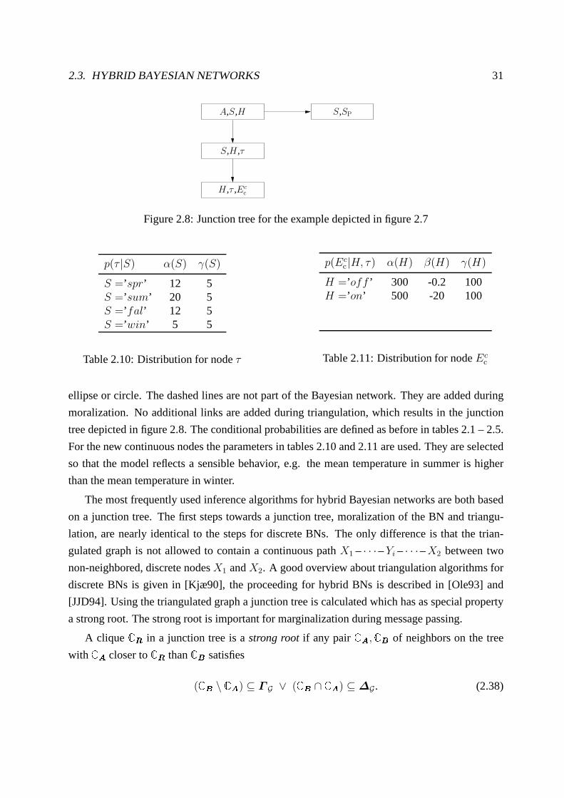
2.3. HYBRID BAYESIAN NETWORKS 31
A,S,H
S,H,τ
H,τ ,Ecc
S,SP
Figure 2.8: Junction tree for the example depicted in figure 2.7
p(τ |S) α(S) γ(S)
S =’spr’ 12 5S =’sum’ 20 5S =’fal’ 12 5S =’win’ 5 5
Table 2.10: Distribution for nodeτ
p(Ecc |H, τ) α(H) β(H) γ(H)
H =’off ’ 300 -0.2 100H =’on’ 500 -20 100
Table 2.11: Distribution for nodeEcc
ellipse or circle. The dashed lines are not part of the Bayesian network. They are added during
moralization. No additional links are added during triangulation, which results in the junction
tree depicted in figure 2.8. The conditional probabilities are defined as before in tables 2.1 – 2.5.
For the new continuous nodes the parameters in tables 2.10 and 2.11 are used. They are selected
so that the model reflects a sensible behavior, e.g. the mean temperature in summer is higher
than the mean temperature in winter.
The most frequently used inference algorithms for hybrid Bayesian networks are both based
on a junction tree. The first steps towards a junction tree, moralization of the BN and triangu-
lation, are nearly identical to the steps for discrete BNs. The only difference is that the trian-
gulated graph is not allowed to contain a continuous pathX1 – · · ·–Yi – · · ·–X2 between two
non-neighbored, discrete nodesX1 andX2. A good overview about triangulation algorithms for
discrete BNs is given in [Kjæ90], the proceeding for hybrid BNs is described in [Ole93] and
[JJD94]. Using the triangulated graph a junction tree is calculated which has as special property
a strong root. The strong root is important for marginalization during message passing.
A cliqueCR in a junction tree is astrong rootif any pairCA,CB of neighbors on the tree
with CA closer toCR thanCB satisfies
(CB \ CA) ⊆ Γ G ∨ (CB ∩ CA) ⊆∆G. (2.38)

32 CHAPTER 2. AN INTRODUCTION TO BAYESIAN NETWORKS
X1 X1
Y1Y1Y2
Y3
Y4
Root R
Figure 2.9: Two cliques with a hybrid separator
X1X1
X2X2
Y1
Y2
Y3
Y4
Y5
Root R
Figure 2.10: Two cliques with a discrete separator
According to Leimer [Lei89] the cliques of a decomposable marked graph can always be
transformed in a junction tree with at least one strong root.
Neighboring cliques which might occur in a junction tree aredepicted in figure 2.9 and 2.10.
In figure 2.8 the cliqueA, S, H can be used as strong root. The separator betweenA, S, HandS, SP is a subset of∆G. WhenS, H, τ = CA andH, τ, Ec
c = CB, the set differenceCB \ CA = H, τ, Ecc \ S, H, τ = Ec
c ⊂ Γ G.
Using a junction tree with strong root guarantees that the separator potentials calculated dur-
ing collectEvidence are always CG-potentials. When calculating the separator potentials in the
other direction usually a CG potential with the same mean anddispersion is used instead.
After the construction of the junction tree, each node of theBN is assigned to one clique
in the junction tree. That means the potential of the node is multiplied with the clique’s po-
tential. The representation of the potential depends on theused inference algorithm. The first
one is described in [Lau92]. It works similarly to the algorithm for discrete BNs; i.e., the joint
distribution is calculated by a division of the clique potentials by the separator potentials. This
algorithm uses two different potential representations atthe same time. The transformation from
one representation scheme to the other includes the calculation of an inverse matrix. Sometimes
this leads to numerical instability. To avoid numerical instability, Lauritzen introduced a second
inference algorithm in [LJ99] which distinguishes betweenso called head and tail variables. A
potential is proportional to a distribution of the head variables given the tail variables.

2.3. HYBRID BAYESIAN NETWORKS 33
2.3.2 Inference in hybrid Bayesian networks
Moment and canonical characteristic
Up to now the strong root of the junction tree is discussed. The junction tree is used by both algo-
rithms. In analogy to discrete BNs, each variableX is assigned to a cliqueC, so thatF(X)) ⊆ C.
The potential of each variable is represented by themoment characteristic; i.e. by its meanξ(x),
the covariance matrixΣ(x), and the probability of the configurationsP (x). The distribution of
continuous nodesY , given the configurationx, is equal to
p(Y | x) = N (ξ(x), Σ(x)) (2.39)
wheneverP (x) > 0. Beside the moment characteristic it is possible to represent a CG-distribution
by thecanonical characteristic, i.e. by a potential
φ(x, y) = χ(x) exp(g(x) + h(x)T y − yT K(x)y/2) (2.40)
whereχ(x) denotes an indicator function which is equal to 1 iffP (x) > 0, andg(x) is a real
number. The length of the vectorh is equal to the length ofy. The symmetric matrixK is
the inverse of the covarianceΣ. Sometimesχ(x) is omitted andP (x) > 0 is required instead.
As both representation schemes are used for different operations during inference process, a
transformation
P (x) ∝ (det (Σ(x)))12 exp(g(x) + h(x)T Σ(x)h(x)/2) (2.41)
ξ(x) = K(x)−1h(x) (2.42)
Σ(x) = K(x)−1 (2.43)
K(x) = Σ(x)−1 (2.44)
h(x) = K(x)ξ(x) (2.45)
g(x) = log(P (x)) +log(det(K(x)))− | Γ | log(2π)− ξ(x)T K(x)ξ(x)
2(2.46)
between the moment and the canonical characteristic has to be defined. The number of continu-
ous nodes in the potential is denoted by| Γ |.

34 CHAPTER 2. AN INTRODUCTION TO BAYESIAN NETWORKS
Initialization
The canonical characteristic is used for initialization
g(x) = −α(x)2
2γ(x)− log(2πγ(x))
2(2.47)
h(x) =α(x)
γ(x)
(1
−β(x)
)(2.48)
K(x) =1
γ(x)
(1 −β(x)T
−β(x) −β(x)β(x)T
)(2.49)
using the parameters given by the definition of the BN.
During the initialization of the junction tree in figure 2.8 the random variableEcc has to
be assigned to the cliqueH, τ, Ecc. This clique is the only one which contains the parentsP(Ec
c) = H, τ. The nodeτ has to be assigned to the cliqueS, H, τ. For the initialization
of φH,τ,Ecc the distributionN (Ec
c |H, τ) is transformed in a potential. Using the parameters of
table 2.11 results in the following canonical characteristic for the potentialφH,τ,Ecc.
g(H = ′off ′) = − 3002
2 · 100− log(2π · 100)
2= −450− 3.22 = −453.22
h(H = ′off ′) =300
100
(1
0.2
)=
(3
0.6
)
K(H = ′off ′) =1
100
(1 0.2
0.2 −0.04
)
=1
100
(0.01 0.002
0.002 −4 · 10−4
)
Provided the domainsDom(φ1) = Dom(φ2) of two arbitrary potentialsφ1 andφ2 are equal,
the canonical characteristic can be used directly for the multiplication and division of potentials
(g1, h1, K1)× (g2, h2, K2) = (g1 + g2, h1 + h2, K1 + K2) . (2.50)
Usually the precondition of equal domains is not given, thusanexpansionof the potentials from
2.3. HYBRID BAYESIAN NETWORKS 35
e.g.φX1,Y 1(x1, y1) to φX1,X2,Y 1,Y 2(x1, x2, y1, y2)
gX1,X2,Y 1,Y 2(x1, x2) = gX1,Y 1(x1) (2.51)
hX1,X2,Y 1,Y 2(x1, x2) =
(hX1,Y 1(x1)
0
)(2.52)
KX1,X2,Y 1,Y 2(x1, x2) =
(KX1,Y 1(x1, x2) 0
0 0
)(2.53)
may be necessary to guarantee equal domains. Using expansion and multiplication, an initial
potential of all cliques in the junction tree is calculated.The separators are initialized with
φS = 1, i.e.φS = (0, 0, 0).
In the junction tree depicted in figure 2.8 the three variables A, S, andH are assigned to
the cliqueA, S, H. This clique has to distinguish 16 different characteristics (g, h, K), one
for each configuration. For the configurationA =’yes’,S =’spr’ , H =’on’, the new potential
φ∗A,S,H is
φ∗A,S,H = φA(A = ′yes′)× φS(S = ′spr′)×
φA,S,H(A = ′yes′, S = ′spr′, H = ′on′)
= (−1.8971, 0, 0)× (−1.3863, 0, 0)× (−2.3036, 0, 0)
= (−5.586, 0, 0) .
For the other cliques no multiplication is necessary duringinitialization.
Marginalization and message passing
Directly after the initialization, message passing is triggered. For message passing equations
(2.16) and (2.17) are used, but with a changed potential definition in comparison to the discrete
case. According to equation (2.16) marginals have to be calculated during message passing.
Marginalization of a CG-distribution over continuous variables results in a CG-distribution. For
marginalization over a discrete variable, a sum of multipleGaussians with different weights has
to be calculated. The resulting potential is not necessarily a CG-potential. E.g. figure 2.11 shows
a mixture of two Gaussians.
Marginalization of a CG-potential is only guaranteed to result in a CG-potential, if marginal-
izing is carried out over a continuous variable. The marginal φ↓X ,Y 1X ,Y 1,Y 2
= (g′, h′, K ′) of

36 CHAPTER 2. AN INTRODUCTION TO BAYESIAN NETWORKS
−5 −4 −3 −2 −1 0 1 2 3 4 50
0.1
0.2
0.3
0.4
0.5
0.6
0.7
0.8
0.9
N (0, 0.5)
N (3, 0.2)
Figure 2.11: Mixture of two Gaussians
φX ,Y 1,Y 2 = (g, h, K) with
h =
(h1
h2
)K =
(K11K12
K21K22
)
g′(x) = g(x) +| Y 1 | log(2π)− log(det(K11(x))) + hT
1 (x)K11(x)−1h1(x)
2(2.54)
h′(x) = h2(x)−K21(x)K−111 (x)h1(x) (2.55)
K ′(x) = K22(x)−K21(x)K−111 (x)K12(x) (2.56)
is a so calledstrong marginalin contrary to theweak marginalwhere only mean and dispersion
of the overall distribution are preserved.
Marginalization over discrete variables results in a CG-potential only if there are no continu-
ous variables in the domain of the potential or if these continuous random variables are removed
by marginalization first.
When sending messages in the direction of the strong root, a strong marginalization takes
place. Calling distributeEvidence from the strong root, a weak marginalization fromφX1,X2,Y =

2.3. HYBRID BAYESIAN NETWORKS 37
(P, ξ, Σ) to φ↓X1,Y X1,X2,Y = (P ′, ξ′, Σ ′)
P ′(x1) =∑x2
P (x1, x2) (2.57)
ξ′(x1) =∑x2
ξ(x1, x2)P (x1, x2)
P ′(x1)(2.58)
Σ(x1) =
∑x2
Σ(x1, x2)P (x1, x2)
P ′(x1)+
∑x2
(ξ(x1, x2)− ξ′(x1))T (ξ(x1, x2)− ξ′(x1))P (x1, x2)
P ′(x1)(2.59)
may take place, where only the mean and dispersion of the CG-distribution are preserved. After
sending messages in both directions, the junction tree is consistent, i.e. for two neighboring
cliquesC1 andC2 with separatorSφ↓SC1≈ φ↓SC2
(2.60)
holds, where≈ means that the first two moments are identical. After messagepassing is fin-
ished, the cliques represent the true marginals for discrete variables, for the hybrid case it is only
guaranteed that mean and dispersion of a cliqueφCφC ≈ φ↓C (2.61)
are equal to the marginal of the joint potentialφ.
To get the junction tree in figure 2.8 globally consistent, collectEvidence is called. First the
marginalφ∗H,τ = φ
↓H,τH,τ,Ec
cis calculated and assigned to the separator. Directly afterwards the
new separator potentialφ∗H,τ is multiplied withφS,H,τ
φ∗S,H,τ = φS,H,τ × φ∗
H,τ . (2.62)
The division by the old separator potential is omitted here as this potential is initialized to one.
Afterwards the strong rootA, S, H is updated. First the new separator potentials
φ∗S,H = φ
∗↓S,HS,H,τ (2.63)
φ∗S = φ
↓SS,SP
(2.64)
38 CHAPTER 2. AN INTRODUCTION TO BAYESIAN NETWORKS
are calculated. Then the strong root gets the new potential
φ∗A,S,H = φA,S,H × φ∗
S,H × φ∗S . (2.65)
Once again the division by the old separator potential is omitted, as they are equal to 1 directly
after initialization. All the calculated marginals are strong marginals. Considering the property
of the strong root it can be seen that during collectEvidencemarginalization always leads to
strong marginals. During distribute evidence weak marginals occur, whenφ↓H,τS,H,τ is calculated.
Here marginalization over the discrete variableSeason is necessary. In this case a mixture of
eight Gaussians is approximated by a mixture of two Gaussians. An equality of the potentials is
therefore not possible.
Introduction of evidences
The last task is the introduction of evidences. Discrete evidencesX = x are entered by multi-
plication of the potential with an indicator function so that the potential is zero for impossible
configurations. In contrast to discrete evidences, for continuous evidencesY = y all cliquesCwith Y ⊆ C have to be changed. Suppose that a potentialφ = (g, h, K) with
h =
(h1(x)
hY (x)
)K =
(K11 K1Y
KY 1 KY Y
)
is simplified, by enteringY = y. The new potentialφ′ = (g′, h′, K ′) is calculated by removing
the components forY by
g′(x) = g(x) + hY (x)y − KY Y (x)y2
2(2.66)
h′(x) = h1(x)− yKY 1(x) (2.67)
K ′(x) = K11(x). (2.68)
Of course the introduction of evidences leads to a smaller domain of φ′. After entering the
evidence, the junction tree is inconsistent. Thus the functions collectEvidence and distributeEv-
idence must be called again to come to a consistent junction tree. After message passing the
clique potentials are proportional to the marginalized joint distribution.
Unfortunately it turned out that the frequent transformation between moment and canonical
characteristic is numerical unstable due to the matrix inversion. This drawback is avoided in the
inference algorithm introduced in [LJ99]. The main idea is to partition the set of continuous

2.3. HYBRID BAYESIAN NETWORKS 39
H
Ecc
τ 1
Figure 2.12: Equivalent network for the training of the nodeEcc
variables intoheadandtail, so that a potential represents a CG distribution of the headvariables
depending on the tail variables.
2.3.3 Learning the parameters of a hybrid Bayesian network
The aim is comparable to the aim in section 2.2.2, i.e. to learn the parameters of the modeled
distribution. For discrete nodes conditional probabilitytables are learned, the technique is the
same, if no arcsX → Y from discrete to continuous nodes are allowed. For the continuous
nodes the meanα, the weight vectorβ, and the varianceγ are the parameters to be estimated.
If global and local independence of the parameters are supposed, it is sufficient to maximize the
parameters of each family independently. Of course, for theestimation of the instantiation, the
complete Bayesian network has to be used. When assuming thatevery continuous nodeY has
at least one continuous parentZ whose last element is 1, the meanα can be modeled by the last
column of the weight vectorβ.
As an example see figure 2.12 which shows an equivalent network for nodeEcc , where the
meanα is replaced by the weight of the link1→ Ecc .
The distribution of nodeY with discrete parentsX and continuous parentsZ becomes
p(y|x, z) =1√
(2π)γexp(
1
2(y − β(x)T z)γ−1(y − β(x)T z) , (2.69)
whereγ is the variance of the normal distribution. For the more general case of a multidimen-
sional normal distribution see [Mur98a]. For the purpose ofthe thesis one-dimensional distribu-
tions are sufficient.
Using an indicator functionδx(x1) being 1 iff x1 = x and 0 otherwise, the part of the

40 CHAPTER 2. AN INTRODUCTION TO BAYESIAN NETWORKS
ESS Remark
dx ∑Nj=1 δjx with δjx = E[δx(xj)|oj]
SY Y,x ∑Nj=1 δjxEx[(yj)2|oj ]
SZY,x ∑Nj=1 δjxEx[zjyj|oj ] Only if Y has continuous parents
SZZT ,x ∑Nj=1 δjxEx[zj(zj)T |oj ] Only if Y has continuous parents
SY,x ∑Nj=1 δxEx[y|oj] Only if Y has no continuous parents
Table 2.12: Essential Sufficient Statistics for training ofhybrid Bayesian networks
log-likelihood depending on the parameters ofY is
L = log(
N∏
j=1
∏x [p(yj|zj, xj , oj)]δx(xj)) . (2.70)
The vectoro denotes theN observations, but all random variablesy, z andx may be unobserved.
Once again the problem is that an estimation of the parameters requires the knowledge of the
instantiation of the unobserved variables and vice versa. For the solution the EM-algorithm might
be used. It starts with an arbitrary parameter-setθ(0). This is used to calculate the estimated log-
likelihood
L = −1
2
N∑
j=1
E[∑x δx(xj) log(γ(x))+δx(xj)(yj−β(x)T zj)γ(x)−1(yj−β(x)T zj)|oj]. (2.71)
To keep track of theN training examples, theessential sufficient statistics(ESS), listed in table
2.12 are used.
The indexx in Ex is used to denote the expectation given thatX = x. The values used by
these formulas are calculated by enteringo as evidence and then using the junction tree algorithm
to calculate the missing values.
Using the statistics the new estimations
β(x)T = STZY,xS−1
ZZT ,x (2.72)
γ(x) =SY Y,xdx − β(x)T SZZT ,x
dx (2.73)
α(x) =SY,xdx (2.74)

2.3. HYBRID BAYESIAN NETWORKS 41
H τ Ecc 1
’on’ 10 493 1’on’ 13 457 1’off ’ 27 107 1’off ’ 19 209 1’off ’ 22 153 1
Table 2.13: Numbers used for the training of the parameters of nodeEcc
are calculated. The Bayesian network is used to calculate the expected values of the unobserved
random variables given the parameter of the last M-step. These expected values are used to
calculate the ESS. When all training cases are included in the ESS, the parameters are maximized
using equations (2.72) to (2.74), where the last one is used for continuous random variables
without continuous parents. For a discussion of the multidimensional case see [Mur98a].
As an example we regard the training ofEcc , with F(Ec
c) = H, τ, Ecc. To simplify the
example, we assume that all variables are observed so that wecan ignore the other random
variables of the example and one EM-step is sufficient to train the parameters. As training cases
the values in table 2.13 are observed.
The observations of table 2.13 results in the following statistics
dH=′on′ = 2
dH=′off ′ = 3
SY Y,H=′on′ = 4932 + 4572 = 451898
SZY,H=′on′ = [10 1]493 + [13 1]457 = [10871 950]
SZZT ,H=′on′ =
[10
1
] [10 1
]+
[13
1
] [13 1
]=
[269 23
23 2
].
This ESS results in the following new parameters for the nodeEcc
βT
= [−12 613]
γ = 0 .
The results is obviously correct as there are two parametersfor two examples so that a variance
equal to zero meets expectation.

42 CHAPTER 2. AN INTRODUCTION TO BAYESIAN NETWORKS
Xt1 Xt2 Xt3 Xt4
Yt1 Yt2 Yt3 Yt4
Figure 2.13: A Hidden Markov Model as an example of a Dynamic Bayesian network
2.4 Dynamic Bayesian networks
The networks discussed in the previous sections had one common trait, namely there is only one
random variable for each measurement. This is sufficient forsome of the engineering processes
discussed in this thesis, but for many purposes it is not. Particularly for the analysis of time
series, for medical purposes (e.g. the regular measurementof a patients fever), or for dynamic
processes described by differential equations, it is necessary to represent the measured data at
different points in time. So information about the past can be used for the prediction of the future.
The main idea is to represent each point in time by a separate Bayesian network, called time-
slices. These time-slices are linked together by temporal edges (cf. [Kjæ92] [Kjæ93]) or inter
slice connections. Usually the Markov assumption holds
x0, x1, · · · , xt−1⊥⊥xt+1, · · · , xt+k|xt, (2.75)
i.e. the future is conditionally independent of the past given the present. The nodesXt having
links to neighbored time slices are called theinterfacenodes. Kjærulff defines the interface as all
nodes with incoming links from previous time slices [Kjæ92], whereas K. P. Murphy [Mur02]
distinguishes between forward and backward interface where the forward interface of a time-
slice contains all nodes with an edge to the next time-slice.In the backward interface all nodes
with an incoming edge from the previous time-slice are included.
As an example the HMM in figure 2.13 can be regarded. Here the discrete state nodesXt are
in the forward interface of time slicet.
Usually the nodes representing the same random variable at different points in time, e.g. the
nodesYt2 , Yt3 , andYt4 have the same parameters. An exception are sometimes the nodes of the
first time-slice. In figure 2.13Xt1 has no incoming links, thus the node represents a probability
P (Xt1) which is in most of the cases different fromP (Xt|Xt−1), t2 ≤ t ≤ t4. So the first

2.4. DYNAMIC BAYESIAN NETWORKS 43
time-slice represents the a-priori distribution, the other time-slices the distribution of the random
variables at timet, given the information at timet − 1. This leads to the following definition of
a DBN, taken from [Mur02]
A DBN is defined to be a pair (BN1,BN→, where BN1 is a BN which defines the prior and
BN→ is a two slice temporal Bayes net, which definesP (Xt|Xt−1) by means of a DAG as follows
P (Xt|Xt−1) =
nN∏
i=1
P (Xi,t|P(Xi,t)) , (2.76)
whereXi,t is the i-th node at timet. In this definitionX is either a discrete or a continuous
random variable.
There are a lot of different inference algorithms. The simplest one, used for the experiments
discussed in chapter 4, is to unroll the DBN totmax time-slices, so that it becomes a hybrid
Bayesian network as discussed in section 2.3.1 withntstmax nodes, wherents denotes the number
of nodes in each time slice. E.g. figure 2.13 can be regarded asa DBN withnts = 2 unrolled to 4
time-slices. The advantage is that the same inference algorithm as discussed in section 2.3.1 can
be applied. The disadvantage is the fixed number of time slices.
To deal with a varying number of time slices Kjærulff [Kjæ92;Kjæ93] suggests a reorgani-
zation of the junction tree. Murphy discusses several inference algorithms in his thesis [Mur02],
one of them is the interface algorithm. The first step is the organization in a junction tree with the
restriction that all interface nodes are in one clique. Thiscan be forced by adding additional links
to the moralized graph. After triangulation there is one clique which separates the time-slices
from each other. For example see figure 2.14 which shows the junction tree resulting from figure
2.13.
Now each time slice is represented by a junction tree, which contains additional nodes from
the previous time-slice. This junction tree contains exactly one clique which is linked to the
previous time slice and one clique linked to the next time slice. As figure 2.14 shows, the cliques
to the previous and to the next time slice might collapse to one clique.
The interface algorithm starts by calling collectEvidencefor the clique containing the nodes
of the forward interface, first for the junction treeJ1, which represents the nodes of the first time
slice. Afterwards the cliques with the forward interface inJ2 to Jtmax call collectEvidence. This
results in an absorption of knowledge from the previous timeslice.
In the backward pass, the forward interface cliques are calling distribute evidence, starting
in the junction treeJtmax . This step includes the distribution of the knowledge to theprevious
time-slice.

44 CHAPTER 2. AN INTRODUCTION TO BAYESIAN NETWORKS
Xt1
Xt1
Xt1
Xt2
Xt2
Xt2
Xt2
Xt2
Xt3
Xt3
Xt3
Xt3
Xt3
Xt4
Xt4
Xt4
Yt1 Yt2 Yt3 Yt4
Figure 2.14: Junction tree of the HMM in figure 2.13
In our example first collectEvidence is called by the cliquesXt1 , Xt2, Xt2 , Xt3 and fi-
nally by Xt3 , Xt4. This finishes the forward pass. During the backward pass distributeEvi-
dence is called byXt3 , Xt4, Xt2, Xt3 and at the end byXt1 , Xt2.In the discussed example all separators are discrete ones, thus all calculated marginals are
strong. Usually this can not be guaranteed so that week marginals might occur in both the
forward and the backward pass.
In the next section the basics of control theory are introduced. After the introduction to con-
trol theory is finished, the application of dynamic Bayesiannetworks as controller is discussed.

Chapter 3
Control of dynamic systems
The overall aim is to study the question whether Bayesian networks can be used for control
purposes. To show the limits and preconditions for the usageof Bayesian controller, this chapter
starts with a characterization of dynamic systems. Afterwards linear systems, together with the
theory of Kalman Filters, are discussed. The knowledge about linear systems leads to a general
structure of Bayesian networks and suitable parameter settings. For non-linear units, prototypical
models are provided for some frequently occurring transferunits. For a discussion of non-linear
systems see section 3.2. In section 3.3 traditional controlmethods and criteria to judge the quality
of control are introduced. These criteria allow a comparison between traditional and Bayesian
controller.
Generally each dynamic system, denoted as transfer unitϕ, maps an input functionu(t) to
an output functionym(t)
ym(t) = ϕ[u(t)]. (3.1)
Firstly, we restrict ourself totime invariantsystems. In time invariant systems a delayed input
signalu(t− t0) leads to the same, delayed output signal
ym(t− t0) = ϕ[u(t− t0)]. (3.2)
Even if equation (3.2) does not hold exactly, it is a common approach in parameter estimation
to assume time invariance. In practice this leads to satisfying results, if changes of the plant are
much slower than the adaptation of the controller (cf. [SL91]). Thus, from now on it is assumed
that dynamic systems are time invariant.
The second property of dynamic systems, which simplifies analysis and control, islinearity.
45

46 CHAPTER 3. CONTROL OF DYNAMIC SYSTEMS
A transfer unitϕ is linear if and only if for arbitrary constantsc1 andc2
ϕ[c1u1(t) + c2u2(t)] = c1ϕ[u1(t)] + c2ϕ[u2(t)] (3.3)
holds.
In the next two sections the descriptions of linear and non-linear systems, as they are usually
used in control theory, are discussed. The aim of the discussion is to guarantee that the new
approach, introduced in this thesis, is applicable to a widerange of systems. The main idea is
to model typical linear and non-linear systems, and show howthese systems respectively the
developed models may be combined to more complex systems.
The knowledge about typical non-linear units also demonstrates the theoretical limits of
Bayesian models for the modeling of dynamic processes. Of course these limits are not iden-
tical with the limits of a stochastic approach in general, asBayesian networks are restricted to
a mixture of Gaussians. Using particle filters [TL98; IB98] may open a complete new range of
applications.
3.1 Description of linear dynamic systems
This section discusses two different approaches for the mathematical description of linear, dy-
namic systems. Both of them correspond to a special Bayesiannetwork. The first discussed
description is the state-space description, which is also used for multiple input multiple output
systems (MIMO). The description by difference equation leads to Bayesian networks with less
hidden nodes and thus shows a better training behavior.
A dynamic system may be regarded as a black box with several input and output signalsu
andym respectively. We distinguish the output of the modelym and the observed outputq, where
the latter includes also the influences of the disturbance variablezd.
The current output of the dynamic system does not depend solely on the input signal, but also
on an internal stateXs or on former in- and output signals. Linear, time invariant systems with
one-dimensional in- and output, are regularly described bydifferential equations
n∑
i=0
aci
diym(t)
dti=
m∑
j=0
bcj
dju(t)
dtj. (3.4)
Only systems withm ≤ n are physical realizable. As a simple example a car with massM ,
accelerated by a forceF and slowed down by friction and a spring, is discussed. The friction is

3.1. DESCRIPTION OF LINEAR DYNAMIC SYSTEMS 47
proportional to the product of a constantb and the velocityv = dsdt
, the excursions of the spring
causes a forceks. Thus
Md2s(t)
dt2+ b
ds
dt+ ks = F (t) (3.5)
holds. By substitutionx1 = dsdt
andx2 = s the example can be transformed to a system of
differential equations of first order
[dx1(t)
dtdx2(t)
dt
]=
[− b
M− k
M
1 0
][x1(t)
x2(t)
]+
[1M
0
]F (t) (3.6)
s(t) = x2(t), (3.7)
or generally
dxs(t)dt
= Axs + Bu(t) (3.8)
ym(t) = Cxs + Du(t) . (3.9)
Equations (3.8) and (3.9) are called the state-space description of a dynamic system. The matrix
A at the left hand side of equation (3.8) describes the trajectory of the statexs. For a homo-
geneous system, i.e.u(t) = 0, the description of the system by the transfer matrixA and the
current statexs0 is sufficient to calculate the state of the system in the future. The influence of the
inputu on the statexs is described by the input matrixB. The first equation of the state-space
description describes therefore the state transition influenced by the inputu.
The modeled output of a system depends in many cases only on the statexs as described by
the output matrixC, for jump Markov systems it depends also on the inputu.
The state-space description is also used to describe multiple-input multiple-output (MIMO)
systems. In the general caseA is an × n matrix, wheren is equal to the order of the system,
the state vectorxs is n × 1 vector. Then × r input matrixB describes the reaction of ther
dimensional input. Theo × n-dimensional output matrixC depends on the dimensiono of the
output. The feedthrough matrixD is of dimensiono× r.
In reality all dynamic systems are exposed to disturbing influenceszd′. For linear systems
it is possible to add the system’s reaction to all disturbance variables to one variablezd which
has an effect on the output of the system. Thus the observed outputq is the sum of the model’s
output and the disturbance variable.
q(t) = ym(t) + zd(t) (3.10)

48 CHAPTER 3. CONTROL OF DYNAMIC SYSTEMS
Time (sec.)
Am
plitu
de
Step Response
0 0.2 0.4 0.6 0.8 1 1.20
0.5
1
1.5
2
2.5
Figure 3.1: Step response of a second order system
The dynamic system is displayed as dashed box in figure 3.7. The manipulation reaction de-
scribes the response of the system to the input signalu(t), e.g. the reaction to the impulse func-
tion. Mathematically the manipulation reaction can be described by the state-space description.
The disturbance reaction defines the reaction on, usually uncontrolled, environmental influ-
enceszd(t). It is the task of a controller to reduce the effect of a disturbance as fast as possible.
To get a good impression of a dynamic system, it is helpful to regard the response to different
input signals, e.g. thestep function
σ(t) =
0 if t < 0
1 if t ≥ 0(3.11)
or theimpulse function
u(t) =
1δ
if 0 ≤ t < δ
0 if t ≥ δ, (3.12)
which can approximately be regarded as a very short impulse of durationδ. Figure 3.1 displays
the step response of a system described by2u(t) = ym + 0.1dym
dt+ 0.01d2ym
dt2which is one of
our test systems. The impulse response of the same system is shown in figure 3.2. A second
order system may overshoot and needs a long time to converge to a new value. In this thesis we
will show how to calculate an input signal, so that overshooting is avoided and the output settles
quickly to its new value. This method is based on Kalman filters as described in section 3.1.2.

3.1. DESCRIPTION OF LINEAR DYNAMIC SYSTEMS 49
Time (sec.)
Am
plitu
de
Impulse Response
0 0.5 1 1.5 2−2
0
2
4
6
8
10
12
Figure 3.2: Impulse response of a second order system
The example of a second order system is now used to discuss thenatural angular frequency
and the dampingD of a dynamic system. Generally, a second order delay elementis described
by
Ksu(t) = T 22
d2ym(t)
dt2+ T1
dym(t)
dt+ ym(t) . (3.13)
The factorKs describes the gain of the system, that is the quotient of the output by a constant
input signal.T1 andT2 are two time constants. The ratio ofT1 andT2 describes thedamping
ratio [LW00; Unb97a]
D =T1
2T2
. (3.14)
Thenatural angular frequency
ω0 =1
T2(3.15)
describes the oscillation behavior. For an undamped system, i.e.D = 0, theresonance frequency
ωr = ω0
√1− 2D2 (3.16)
is equal to the natural angular frequency.
According to the damping five different systems are distinguished. They show different step
responses.
Overdamped systems withD > 1 converge to their new output without any overshoot. There

50 CHAPTER 3. CONTROL OF DYNAMIC SYSTEMS
0 0.5 1 1.5 2 2.5 3 3.5 4 4.50
0.2
0.4
0.6
0.8
1
1.2
1.4
Ks
Tu Ta
Am
plit
ud
e
Time(sec.)
Step Response
Figure 3.3: Calculation of delay timeTu and raise timeTa
are different parameters to characterize overdamped systems. E.g. the step response is character-
ized by the gainKs, the delay timeTu, and the rise timeTa. The time constantsTu andTa are
calculated as depicted in figure 3.3. In a simple approach by Ziegler and Nichols they are used
to determine the parameters of a controller.
Critically damped systems withD = 1 show a faster increase of the output than systems with
higher damping. If the dampingD is between 0 and 1, an overshoot together with an oscillation
with decreasing amplitude is observed, as shown in figure 3.1. When a damping of 0 is reached
the amplitude of the oscillation keeps constant. Further decreasing of the damping to a value
between -1 and 0 leads to an unstable system whose step response has an increasing amplitude.
For the more general case ofn-th order system theLaplace transformationis helpful which
maps a functionf(t) to
F (s) =
∫ ∞
0
f(t) exp(−st)dt . (3.17)
The quotientG(s) of the Laplace transformed out- and input signalY m(s) respectivelyU(s)
G(s) =Y m(s)
U(s)(3.18)
is calledtransfer functionof the dynamic system. Linear single-input single-output(SISO) sys-

3.1. DESCRIPTION OF LINEAR DYNAMIC SYSTEMS 51
tems are described by
G(s) =bc0 + bc
1s + · · · bcmsm
ac0 + ac
1s + · · ·+ acnsn
=B(s)
A(s)(3.19)
the quotient of two polynomialsA(s) andB(s).
Sometimes the described system reacts with a delayTd, calleddead-time, to changes of the
input. This is modeled by an additional terme−Td , so that
G(s) =B(s)
A(s)e−Td . (3.20)
Please note thatA(s) andB(s) are used for the description of the system, whereasY m(s) and
U(s) denote the Laplace-transformed in- and output signals. To get an impression of the behavior
of the dynamic system the homogeneous system, i.e.u(t) = 0, is regarded. In the Laplace
transformed this leads toU(s) = 0 and thus to
A(s) = ac0 + ac
1s + · · ·acns
n = 0 , (3.21)
usually called thecharacteristic equation.
If all zerossk with A(sk) = 0 are in the left half s-plane, i.e. the real partRe(sk) < 0, the
system is stable. If at least onesk has a real partRe(sk) > 0 or if a multiple pole is placed on
the imaginary axis, i.e.Re(sk) = 0, the system is unstable.
In equations (3.8) and (3.9)A is an×n matrix, wheren denotes the order of the differential
equation. For single input single output systems, i.e. bothym andu are scalars instead of vectors,
B andC are vectors of lengthn andD is a scalar. Thus, there aren2 + 2n + 1 parameters in
the state space description. Comparing the number of parameters in the state space description
with the maximal number of parameters in differential equation (3.4) leads to the conclusion that
there are many possible state space descriptions for the same differential equation. Reducing the
number of parameters would result in a smaller search space of possible state space descriptions,
which means a more robust and effective learning process. That is exactly what is done by normal
forms.
3.1.1 Normal forms
As mentioned in the last paragraph of section 3.1, there is nounique state space description for
a given differential equation. As a simple example imagine adynamic system with gainKs. To
model such a system the amplification can either take place between the inputu and the statexs

52 CHAPTER 3. CONTROL OF DYNAMIC SYSTEMS
or between the statexs and the outputym.
Control theory distinguishes several normal forms, usually the form of the matricesA, B, C,
andD makes the difference. As this chapter is no introduction to control theory, only theobserv-
able canonical formis discussed. The reason to use the observable canonical form is of practical
nature and will be explained later.
By a transformation process, defined e.g. in chapter 1.6 of [Unb97b], the matricesA, B, C,
andD take the form
A =
0 0 0 · · · 0 0 −a0
1 0 0 · · · 0 0 −a1
0 1 0 · · · 0 0 −a2
. . . . . . . . . . . . . . . . . . . . . . . . . . . . . .
0 0 · · · 1 0 −an−2
0 0 · · · 0 1 −an−1
B =
b0
b1
...
bn−1
C = [0 0 0 · · ·1] D = bn .
(3.22)
It is important to note that the introduction of normal formsis neither a restriction of the dynamic
system, nor is the input/output-behavior of the system changed. Only the internal state of the
system is concerned. Using the observable canonical form the number of free parameters is
reduced to2n + 1. This number is equal to the number of parameters in the differential equation
(3.4), provided thatn = m andan is normalized to 1. So no redundancy is left.
Up to now only the description of systems in continuous time space is discussed. The next
section 3.1.2 describes the transformation to discrete time domain. This transformation is also
suitable to deduce the weights of a DBN, modeling the system.
3.1.2 Kalman filter
For digital control the output signalsq(t) are not measured for all points in time, usually the
measurements are taken regularly with a fixed sampling period ∆T . The same is valid for the
input signalu(t), which is only calculated for special points in time. Between two pointt and
t + 1 it is assumed thatut is constant, i.e.u(τ) = ut for t ≤ τ < t + 1. Linear time discrete
systems are described in the same way as continuous time systems, only the coefficients have
to be changed. The coefficients are deduced by comparison to Kalman filters, a well-known
method for tracking and prediction of stationary, linear systems. It can be used to calculate
the parameters of time discrete systems as described in section 3.1, equations (3.8) and (3.9).

3.1. DESCRIPTION OF LINEAR DYNAMIC SYSTEMS 53
Furthermore Kalman filters are a special case of DBNs, so the results obtained for Kalman filter,
e.g. in [Gel94], may be used without any changes.
Kalman filters represent a time discrete system whose state transition
xst+1 = ABNxs
t + BBNut (3.23)
is described by the matrixABN. In this equationt is used as index to denote a time discrete
system. The index ’BN’ is used, as the transfer matrices are different for time discrete systems.
To calculateABN, a solution of differential equation (3.8) is needed, asABN has to integrate
all the state transitions betweent and t + 1. As long as no input is present, equation (3.8) is
solved by
xs(t) = xs(t0)Φ(t, t0) (3.24)
where
Φ(t, t0) =∞∑
i=0
Ai (t− t0)i
i!(3.25)
is called transfer matrix. Assumingt = tk+1 and t0 = tk with a constant time difference
∆T = tk+1 − tk the matrix
ABN = Φ(tk+1, tk) (3.26)
depends only on the time difference∆T andA. ThusABN is constant for allk; i.e., the param-
eters of a DBN, modeling the dynamic system, are independentfrom the time slice.
Taking into account the influence of the input on the state leads to
BBNut =
∫ tk+1
tk
Φ(tk+1, τ)Bu(τ)dτ (3.27)
which simplifies to
BBN = ∆T
∞∑
i=0
Ai∆T i
(i + 1)!B (3.28)
if only systems with a constant sampling period∆T = tk+1− tk and a constant inputut = u(τ)
within one time-slice are considered. To build a DBN which incorporates equations (3.26) and
(3.28),BBN is used as weight matrix between the input nodes and the statenodes as shown in
figure 3.4. MatrixΦ(∆T ) describes the transition from one state to the next and is therefore used
as weight matrix for the inter slice connection between two states in neighboring time slices. This

54 CHAPTER 3. CONTROL OF DYNAMIC SYSTEMS
ut ut+1
BBN(Φ, B)
x1,t
x2,t
x1,t+1
x2,t+1
Φ(A, ∆T )
ymt ym
t+1
CC
t t + 1
Figure 3.4: Bayesian network used for modeling the state transition
means that the state at timet + 1 is calculated by
xst+1 = [Φ(∆T ) BBN] ·
[xs
t
ut
]. (3.29)
In a BN the meanξ of the normal distribution is equal toξ = α + βz. In contrast to equation
(2.37), describing the one-dimensional case,α is a vector, andβ is a matrix.
The offsetα has to be set to zero and the weights of the state nodeXs are set to
β = [Φ(∆T ) BBN] , (3.30)
so that the weights of the state nodes reflect the state transition in the presence of inputu. The
output depends linearly on the state and is not time dependent. Thus the matrixC andD remain
unchanged also in a time discrete system. Figure 3.4 shows two time-slices of a linear DBN.
The nodes of the net are pictured as circles, the rectangles are used to display the weights of the
Bayesian net. It is assumed that the modeled system is no jumpMarkov system, i.e.D = 0.
As a further consequence, the dimension of the hidden state nodes is equal to the order of the
differential equation describing the system.

3.1. DESCRIPTION OF LINEAR DYNAMIC SYSTEMS 55
3.1.3 Description of dynamic systems by difference equation
In the state-space description (3.8) and (3.9) the statexs usually cannot be observed. Even
if the parameters of a Bayesian network can be trained despite the occurrence of unobserved
variables, it is more cumbersome. According to our experience, the number of needed iterations
and examples is higher in the presence of unobserved variables. Thus it would be desirable to
model with a description without hidden variables.
The starting point is again the description by differentialequation (3.4). The derivatives of a
functionf can be approximated by the finite differences
df
dt
∣∣∣∣t=k∆T
≈ f(k∆T )− f([k − 1]∆T )
∆T(3.31)
d2f
dt2
∣∣∣∣t=k∆T
≈ f(k∆T )− 2f([k − 1]∆T ) + f([k − 2]∆T )
∆T 2(3.32)
d3f
dt3
∣∣∣∣t=k∆T
≈ f(k∆T )− 3f([k − 1]∆T ) + 3f([k − 2]∆T )− f([k − 3]∆T )
∆T 3. (3.33)
Derivatives of higher order are approximated in a similar manner. Thus it is possible to rewrite
equation (3.4) using expressions (3.31) to (3.33) instead of the derivatives. This procedure results
in a difference equation which can be solved for
ym = −n∑
i=1
aiymt−i +
n∑
i=0
biut−i−d , (3.34)
with d = Td
∆Tas the discrete dead-time. Please note that the coefficientsin equations (3.4) and
(3.34) are different, the coefficients for the time continuous system are marked by the superscript
c. It is not possible to rewrite the differential equation to adifference equation without adapting
the coefficients1. As only the structure will be used, a description of the transformation algorithm
is omitted. The available algorithms are discussed e.g. in [Sch02].
In analogy to the description of dynamic systems by the Laplace transformation, time discrete
systems are often described by theZ-transformationof a functionf(k)
Zf(k) = F (z) =
∞∑
k=0
f(k)z−k . (3.35)
1For a transformation the Z-transformation might be used.
56 CHAPTER 3. CONTROL OF DYNAMIC SYSTEMS
For single input single output systems the Z-transformation leads to a transfer function
G(z) =Y m(z)
U(z)=
b0 + b1z−1 + · · · bnz−n
1 + a1z−1 + · · ·anz−nz−d . (3.36)
Once again the system is described by two polynomialsA(z) = 1 + a1z−1 + · · ·anz
−n, and
B(z) = b0 + b1z−1 + · · · bnz
−n, and the dead timed.
The description by Z-transformation has similar advantages as the Laplace transformation;
e.g., the convolution integral, which is used to calculate the output of the serial connection of two
systems, is mapped to the multiplication of the two Z-transfer functions. Similarly, the addition
of two z-transfer functions is used to calculate the output of two parallel systems.
The difference equation (3.34) can also be used for estimation of the parametersai andbj . As-
suming that there aren+N−1 input- output pairsut−n+1, ut−n+2 · · ·ut+N−1, qt−n+1, · · · , qt+N−1,
the errorǫt+j between the observed valueqt+j and the predicted values is, according to equation
(3.34), equal to
ǫt+j = qt+j−qt+j−1a1−qt+j−2a2 · · ·−qt+j−nan +ut+j−1a1 +ut+j−2a2 · · ·+ut+j−nan . (3.37)
For all ǫt+1 · · · ǫt+N this results in a system of N linear equations
ǫt+1
ǫt+2
...
...
ǫt+N
=
qt+1
qt+2
...
...
qt+N
−
qt · · · qt−n+1 ut · · · ut−n+1
qt+1 · · · qt−n+2 ut+1 · · · ut−n+2
......
......
qt+N−1 · · · qt−n+N ut+N−1 ut−n+N
a1
...
an
b1
...
bn
(3.38)
or shorterǫ(N) = q(N)−M (N)Ξ(N). The matrixM denotes the matrix for the observations
of the input- and output values. It is necessary to solve thisequation for the parameter vectorΞ.
This can be done by the least square approach, the sum of the squared error is minimized by
Ξ =[M (N)TM(N)
]−1M(N)q(N) . (3.39)
The approach just discussed is only valid for white noiseǫ. In the case of colored noise, there is
no closed solution; a possible approach is e.g. gradient descent or the EM-algorithm. This case
is discussed more deeply in [Unb97a].
3.2. NON-LINEARITIES IN DYNAMIC SYSTEMS 57
The estimation of the control parameters may lead to a self-tuning controller whose basic
principle is the identification of the system in the first stepand the calculation of the controller’s
parameters in dependence of the plant model in a second step.
3.2 Non-Linearities in dynamic systems
For linear systems, discussed in the last section, equation(3.3) hold. All other systems are called
non-linear. In this section an overview about frequently occurring non-linear units in control
theory is given. Later on this list will be used to develop prototypical models for as many non-
linear units as possible. The prototypical models can be combined among each other or with a
linear sub-system. According to [SL91] the decomposition of a system in a linear and a non-
linear subsystem is often possible and useful.
When analyzing non-linear systems the Laplace transformedis no longer the quotient of two
polynomials. But it is still possible to characterize them by two differential equations
xs = f(xs, u, t) (3.40)
ym = g(xs, u, t) (3.41)
with arbitrary non-linear functionsf andg, and the initial state
xs(t0) = xs0 . (3.42)
The state-space description of linear systems is a special case of differential equations (3.40)
and (3.41). For modeling purposes and to analyze the behavior of dynamic systems, differential
equation (3.40) may be linearized by a Taylor series. The operating pointxs, u is usually an
equilibrium point; i.e., the derivative of the state is zero. Thusf (xs, u, t) = 0. Using the
substitutions
∆xs(t) = xs(t)− xs (3.43)
∆u(t) = u(t)− u (3.44)
to denote the deviation from the operating point, differential equation (3.40) is approximated by
∆xs ≈ A∆xs + B∆u (3.45)

58 CHAPTER 3. CONTROL OF DYNAMIC SYSTEMS
whereA andB denote the Jacobian matrices
A =
∂f1(xs,u)∂xs
1· · · ∂f1(xs,u)
∂xsn
......
∂fn(xs,u)∂xs
1· · · ∂fn(xs,u)
∂xsn
xs = xs
u = u
(3.46)
B =
∂f1(xs,u)∂u1
· · · ∂f1(xs,u)∂ur
......
∂fn(xs,u)∂u1
· · · ∂fn(xs,u)∂ur
xs = xs
u = u
. (3.47)
For a discussion see [Unb97a]. In this case the system can be modeled approximately as de-
scribed in section 3.1. If linearization is no solution to the modeling problem, special solutions
for each data set or rather engineering process have to be developed. In many cases common
transfer units are met [Fol93; SL91; Unb97b]. In this section some of them are introduced. In
section 5.1 Bayesian networks are introduced to model thosenon-linear units.
A common phenomenon in engineering issaturation. When a valve is closed, further dimin-
ishing the pressure has no effect. The same happens in an amplifier. For very high inputs the
maximal output is reached. Further increasing the input does not change the output. Assuming a
linear gain between minimal and maximal output, this type ofnon-linear unit is described by
ym(u) =
−ymmax if u ≤ −usat
ymmax
usatu if −usat ≤ u ≤ usat
ymmax if u ≥ usat
(3.48)
This function consists of three different linear parts, so afirst approach for modeling might be
a discrete node with three states as a switch. This switch is parent of a continuous node which
models the output.
Another non-linear unit, which might be applied as a simple temperature controller is the
two-point element
ym(u) =
−ym
max if u < 0
ymmax if u > 0
. (3.49)
Another possibility to express this relationship between in- and output is
ym(u) = −ymmax sgn(u) (3.50)

3.2. NON-LINEARITIES IN DYNAMIC SYSTEMS 59
When using this unit as a controller the input of the system isu(t) = ymmax sgn(w(t)− q(t)); i.e.,
the input is positive if the desired value is greater than thecurrent value and vice versa. When
systems with dead-timeTd has to be controlled an oscillation with the angular frequency
ω0 =π
2Td(3.51)
[Unb97b; Fol93] is observed. Thus, for systems with no or low dead time, a controller which
reacts only when the deviation from the desired value is larger than a thresholduΘ is from
advantage. Thus athree-point controllerwith three possible outputs−ymmax, 0, y
mmax
ym(u) =
−ymmax if u < uΘ
0 if −uΘ ≤ u ≤ uΘ
ymmax if u > uΘ
(3.52)
might be used for control purposes. It is possible to represent it by two two-point elements:
ym1 (u) =
ymmax
2+
ymmax
2sgn(u− uΘ) (3.53)
ym2 (u) = −ym
max
2+
ymmax
2sgn(u + uΘ) (3.54)
ym(u) = ym1 (u) + ym
2 (u) =ym
max
2(sgn(u− uΘ) + sgn(u + uΘ)) . (3.55)
A similar behavior is shown by the next function which shows adead zonebetween the
thresholds−uΘ anduΘ. For inputs smaller or greater than the thresholds the output
ym(u) =
ms(u + uΘ) if u ≤ −uΘ
0 if −uΘ < u < uΘ
ms(u− uΘ) if u ≥ uΘ
(3.56)
is also proportional to the slopems (confer figure 3.5).
Up to now all the introduced non-linearities consist of multiple lines. Of course this is not
valid for all non-linearities. Simple counter-examples are
ym(u) = u2 (3.57)
or arbitrary non linear functions, e.g. the dependency between volume and pressure in hydro-
forming.

60 CHAPTER 3. CONTROL OF DYNAMIC SYSTEMS
−6 −4 −2 0 2 4 6−3
−2
−1
0
1
2
3
u
ym
(u)
Figure 3.5: Dead zone
ym
uuΘ
ymmax
−uΘ
−ymmax
Figure 3.6: Hysteresis
Another class of non-linearities depends not only on the input, but also on the first derivative,
e.g. the input/output dependency depicted in figure 3.6. There is no unique output foruΘ ≤u(t) ≤ uΘ. Thehysteresiswas first observed in magnets, the function is equal to
ym(u, u) =
−ymmax if u < −uΘ
ymmaxsgn(u− ym
maxsgn(u)) if −uΘ ≤ u ≤ uΘ
ymmax if u > uΘ
. (3.58)
If more than one input is used also the multiplication or division of two signals is non-linear. Of
course this list is not complete. But it allows to draw some conclusions. To model non-linearities
with multiple lines or the dependency of the derivative of the input signal it is important to model
the sgn-function.
For the general caseym = f(u) a Taylor series with multiple operating points is applied. The
same approach might also be suitable for
ym = u1(t)u2(t) (3.59)
with operating pointsu1 andu2
ym ≈ u1u2 +∂ym
∂u1
∣∣∣∣u1=u1u2=u2
+∂ym
∂u2
∣∣∣∣u1=u1u2=u2
. (3.60)
A direct representation with hybrid Bayesian networks is not possible, as the mean output of a
continuous node depends linearly on the instantiation of the input nodes.
If the hybrid Bayesian network is inaccurate for the data to be modeled sampling mechanisms

3.3. CONTROLLED SYSTEMS 61
like particle filters might be used. E.g. BUGS, a system basedon Gibbs-sampling [STBG96a;
STBG96b; STBG96c], allows the usage of deterministic nodesand non-Gaussian distributions.
But the disadvantage is that there are no inference mechanisms with a closed solution for the
general case.
Another problem in dealing with non-linearities is the detection of equilibrium points with
xs = 0. In linear systems
xs = Axs + BBNu = 0⇒ xs = A−1BBNu (3.61)
there is one equilibrium point for systems withdet(A) 6= 0. For systems withdet(A) = 0
there might be an infinite number of equilibrium points or none. The latter case is impossible for
u = 0. For the non-linear case multiple equilibrium points can occur.
In the next section two different approaches for control, which calculate the input signals
using the deviation of the current output from the desired value, are introduced. First PID con-
trollers, which are widely used in industry, are discussed.The second approach are Dead-Beat
controllers which guarantee a minimal settling time. For additional approaches see [Unb97a;
Sch02].
3.3 Controlled systems
The aim of a controller is to change the inputu of a dynamic system so that the output of a
system is kept close or equal to the desired value. A simple example is the room-temperature,
controlled by the heating. Here the desired valuew is the favorite temperature of the inhabitants.
This temperature should be kept constant despite disturbances, e.g. opened doors or windows.
Usually the controller is driven by the error, the difference between the desired value and the
output.
In section 1.2 approaches, usually referred to as intelligent control, are discussed. This sec-
tion deals with traditional approaches, i.e. PID- and Dead-Beat controllers.
Additionally, several criteria are developed to judge the performance of the controller dis-
cussed in this section and the Bayesian controller in chapter 4.
The main elements of a control loop are depicted in figure 3.7 where all variables are assumed
to be one-dimensional. The desired valuew is compared with the outputq of the system; e.g.
the current temperature is compared with the desired one.
The difference between desired and current valuee is used as input for the controller which

62 CHAPTER 3. CONTROL OF DYNAMIC SYSTEMS
Measurement
Disturbance reaction
ActuatorController Manipulation reaction
Controlled System
e ymu
zd
w
q
zd′
+ ++-
Figure 3.7: Block diagram of a controlled system
calculates the input for the actuator. The changed input value of the dynamic system results in a
new output. Themanipulation reactiondescribes how the system responds to new inputs. The
manipulation reaction can e.g. be described by a differenceequation or the state-space description
as discussed in section 3.1. A crucial feature of control is the feedback loop which compares the
output with the desired value.
Additionally, the controller has to deal with multiple disturbanceszd′
i (t) from the environ-
ment. In a detailed approach the effect of each disturbance has to be modeled by its own transfer
function, but for linear systems it is possible to substitute the effect of all disturbances by one
disturbance variable
Z(s) =∑
i
Gi(s)Zi(s) (3.62)
which is added to the output. This model is similar to the approach used for system identification.
From now onzd is added to the outputym so thatq(t) = ym(t) + zd(t).
In many cases controllers use the errore(t) = w(t) − q(t) as input, a model of the dynamic
system is not needed. To judge the performance of a controller there are several measures. The
selection of a suitable measure depends on the application.The integral over the squared error
I =
∫ ∞
0
(e(t)− e∞)2dt (3.63)
is frequently used, wheree∞ denotes the steady state error; i.e., the error which remains after
convergence to a steady state. In digital control the error is only known for special points in time
so that the squared error sum
Id =tconv∑
t=0
∆T (et − e∞)2 (3.64)
is used instead of the integral. Summation is stopped attconv when all signals are converged to

3.3. CONTROLLED SYSTEMS 63
their final value. For practical reasons, convergence is assumed when all changes in the last 25
time slices are smaller then10−4.
The next section explains the function of a PID controller which is very popular in industry.
As second controller type also the Dead-Beat controller is defined. The Dead-Beat controller is a
digital filter which guarantees minimal settling time. As drawback a mathematical model of the
dynamic system is required for parameter setting of the filter.
3.3.1 Different types of controllers
The task of a controller is to minimize the effects of an occurring disturbance. Widely used are
PID controllers which have an output proportional to the error and to the integral/derivative of
the error. There are different approaches for the selectionof the controller-parameters depending
on the user’s requirements. When the mathematical description of the plant is given, a calcu-
lation which minimizes the squared error, as defined by equation (3.63) (for the calculation see
[Unb97a]), or the settling time might be used. For a discussion of techniques from artificial
intelligence see section 1.2.
This section starts with the discussion of thePID controller. Afterwards one method for
the selection of the parameters which minimizes the settling time is given. It presupposes a
mathematical description of the plant. If the plant parameters are unknown parameter estima-
tion might be used, e.g. the EM algorithm. These considerations lead to the first type of self
adaptive controllers, known asself tuning controllers(STC), which estimate the plant’s param-
eters and calculate the controller’s parameters accordingly. This approach is opposed to the
model-reference adaptive controller(MRAC) which uses a reference model to specify the ideal
response of the adaptive control system. The adaptation of the controller’s parameters has the
aim to approximate the reference model.
PID controller
A PID controller consists of three different parts, some of them may be missing. The (P)roportional
part of a PID controller leads to an output
u(t) = Kce(t) (3.65)
proportional to the error and to the gain of the controllerKc. Exceptionally, the output is de-
noted byu(t) as the controller’s output is usually used as the input of thedynamic system. The

64 CHAPTER 3. CONTROL OF DYNAMIC SYSTEMS
disadvantage of a pure P controller is the remaining steady state error which is proportional to
e∞ =1
1 + K0wσ(t) (3.66)
when the input is proportional to the step functionσ(t). The closed loop gainK0 = KcKs is the
product of the controller’s gainKc and the plant’s gainKs.
To avoid the steady state error, an (I)ntegral part, whose output
u(t) =Kc
TI
∫ t
0
e(τ)dτ (3.67)
U(s) =Kc
TIsE(s) (3.68)
is proportional to the integral of the error, is added. The outputu(t) of the integral part depends
on the integral timeTI . Both the controller gainKc and the integral timeTI are used to adapt the
PI-controller to different dynamic systems. The PI-controller reduces the steady state error for a
disturbancezd(t) = zd0σ(t) to zero.
To reduce the overshoot, a control signal
u(t) = KcTDde(t)
dt(3.69)
U(s) = KcTDsE(s) (3.70)
proportional to the derivative of the error is used. The (D)erivative part is governed by the
derivative time constantTD. So a PID controller, which combines all three parts, has theoutput
u(t) = Kce(t) +Kc
TI
∫ t
0
e(τ)dτ + KcTDde(t)
dt. (3.71)
As it is impossible to realize a pure D controller, a DT1 unit with
U(s) = KcTDT1s
1 + T1sE(s) (3.72)
is used. Its behavior depends on the one hand on the derivative time constantTD and on the other
hand on the time constantT1.
In most of the cases the controller uses the errore(t) = w(t) − q(t) as input signal which
results in the control loop depicted in figure 3.8 with

3.3. CONTROLLED SYSTEMS 65
ym(t)u(t)
zd(t)
w(t)G(s)Gc(s) +
++
-
Figure 3.8: Typical control loop
Y m(s) = Zd(s) + [W (s)− Y m(s)]Gc(s)G(s) (3.73)
Y m(s) =1
1 + Gc(s)G(s)Zd(s) +
Gc(s)G(s)
1 + Gc(s)G(s)W (s) . (3.74)
Neglecting the disturbance variable, equation (3.74) leads to
Y m(s) =Gc(s)G(s)
1 + Gc(s)G(s)W (s) (3.75)
or to the control transfer function
Gw(s) =Y m(s)
W (s)=
Gc(s)G(s)
1 + Gc(s)G(s)(3.76)
which reflects the reaction of the system, when the desired value is changed. This equation can
be used to calculate the transfer function of the controllerGc(s)
Gc(s) =1
G(s)
Gw(s)
1−Gw(s), (3.77)
provided that the desired command response is known.
A similar equation in the discrete time domain can be used to figure out controller settings
for a filter, which guarantees that the new desired value is reached within finite time. This filter,
called Dead Beat controller, is discussed in the next section.
Dead Beat Controller
In digital control an equation similar to (3.77)
Gc(z) =1
G(z)
Gw(z)
1−Gw(z), (3.78)

66 CHAPTER 3. CONTROL OF DYNAMIC SYSTEMS
is used. The only difference is that z-transformation is used instead of Laplace-transformation.
To design a controller, the control transfer functionGw(z) is assumed to be equal to the desired
control transfer functionFw(z). Thus the controller results in
Gc(z) =1
G(z)
Gw(z)
1−Gw(z)=
A(z)
B(z)z−d
Fw(z)
1− Fw(z)(3.79)
whered is the discrete dead-timed = Td
∆T. In order to get a realizable controller the dead-time of
the closed loop is at least the dead-time of the system. Thus the required control transfer function
is restricted to
Fw(z) =K(z)z−d
N(z)(3.80)
whereK(z) andN(z) are arbitrary polynomials, provided thatA(z) andB(z) have only zeros
within the unit circle. That is, equation (3.80) is only applicable for stable systems.
One possible design criterion is that the outputymt is equal to the desired valuewt after a
finite number of time steps. This requirement is expressed bythe restriction ofFw(z) to
Fw(z) = K(z)z−d . (3.81)
This selection guarantees only that the output is equal to the desired value at sampling time.
Therefore stability of the input signals is used as next requirement. The selection
K(z) =B(z)
B(1)(3.82)
guarantees a stable input (for an explanation see [Unb97a; Sch02]) and additionally a minimal
settling time. Together with equation (3.79) this results in
Gc(z) =A(z)
B(1)−B(z)z−d. (3.83)
The approach of a Dead-Beat controller is not restricted to stable dynamic systems. The appli-
cation to unstable systems leads to further restrictions, discussed e.g. in [Unb97a; Sch02].
Not in all cases a mathematical description of the plant is given. An empirical approach was
introduced e.g. by Ziegler and Nichols [ZN42]. Even if strong restrictions apply, it is still very
popular (confer page 246, [Unb97a]). The approach by Ziegler and Nichols is therefore also
compared to the Bayesian controller.

3.3. CONTROLLED SYSTEMS 67
50 50.005 50.01 50.015 50.02 50.025 50.03 50.035 50.04−0.05
0
0.05
0.1
0.15
0.2
Out
put
Time in sec.
Tcrit
Figure 3.9: Output signal forKc = Kcrit
Settings using raise and delay time Controller settings using critical gainType of controller KC TI TD
P 1Ks
Tr
Tu0.5Kcrit
PI 0.9Ks
Tr
Tu3.33Tu 0.45Kcrit 0.85Tcrit
PID 1.2Ks
Tr
Tu2Tu 0.5Tu 0.6Kcrit 0.85Tcrit 0.12Tcrit
Table 3.1: Controller settings based on the methods of Ziegler and Nichols
Empirical approach
Another frequently used method is developed by Ziegler and Nichols. It is valid for systems
approximated by first order systems with dead timeTd
Gs(s) =Ks
1 + T1sexp(−Tds) , (3.84)
which are determined by a time time constantT1, the gainKs and the dead timeTd. The step
response of such systems is characterized by the gainKs, the raise timeTa and the delay time
Tu. The parameter are figured out using the intersection of the tangent with the x-axis and the
line with ym(t) = Ks as displayed in figure 3.3. In [ZN42] the settings given in table 3.1 are
suggested.
A second method, also by Ziegler and Nichols, is based on the measurement of the critical
controller gainKcrit.
Critical controller gain means that the controller gainKc of a P controller is increased until
oscillation is observed, as depicted in figure 3.9. The durationTcrit of the oscillation is measured.
Afterwards the formulas given in table 3.1 are used for adjustment of the parameter.

68 CHAPTER 3. CONTROL OF DYNAMIC SYSTEMS
Chapter 4
Modeling Linear Dynamic Systems with
Bayesian Networks
As seen in chapter 3 automatic control is a field with a long tradition. Also self-adaptive control
has a history of more than 50 years. Of course, self-adaptivecontrol requires a kind of learning
or training algorithm which either refines the adaptation ofthe controller directly, or first im-
proves the model, and afterwards the controller’s parameters depending on it. Frequently used
approaches in adaptive control are neural networks and Fuzzy Logic. Bayesian networks are
seldom used, although they offer a lot of attractive properties for the usage in adaptive control.
The main advantage is the similarity between Kalman filter and DBNs. Thus, a-priori knowl-
edge from control theory can easily be used to deduce the structure and parameters of a suitable
model. Afterwards the Bayesian network is used without any changes to figure out suitable input
for the system to be controlled.
For non-linear systems, there are no models readily available. In principle, there are also
structure learning algorithms, but experience in modelingmanufacturing processes shows that a
lot of know-how about the modeled process is required duringdevelopment of the model.
For the modeling of non-linear systems a strategy that consists of two different steps is sug-
gested in this thesis. Firstly, well known non-linearitiesare modeled. Secondly, the primitive
units developed in the first step can be combined - either by a well informed knowledge-engineer
or by a modified structure learning algorithm - to a complex model. The suggestions for the first
step are described in chapter 5.1, the second step is beyond the scope of this thesis.
In the next section the similarities between Kalman filter and DBNs are used to map the
state-space model to a DBN. As DBNs are not only able to predict results from given inputs, but
also to calculate suitable input signals to obtain a desiredoutput, this model will be used to infer
69

70 CHAPTER 4. MODELING LINEAR DYNAMIC SYSTEMS
suitable manipulated variables, given the desired value.
Additionally the test systems, used to evaluate the new typeof controller, are introduced. In
section 4.2 it is shown how normal forms (confer section 3.1.1) are applied to reduce the search
space for training of Bayesian networks.
The trained models are tested with the same systems as in section 4.1, so that the performance
of the trained model can be compared with the analytical one.The results obtained with this
structure are sufficient in most cases. In one case however, convergence of the output signal is
not achieved. To accomplish convergence in all cases a second structure, based on difference
equations, is tested. When assuming that there is no disturbance during training, there are no
hidden nodes left. Thus greater accuracy is obtained with less training data. The disadvantage of
this model is that the Markov assumption is not met. So most ofthe tools for Bayesian models
are not able to deal with such models directly. A work around is described in section 4.3, the
expansion of the Bayesian toolbox together with the experiments for controlling higher order
systems are described in section 4.4.
As the control with Bayesian networks is a completely new approach, a comparison with
traditional approaches is also necessary. One method, frequently used in industrial control, are
PID controllers. A traditional method for figuring out theirsetting is introduced by Ziegler and
Nichols [ZN42]. A modern mean, used in Digital control, are Dead-Beat [Sch02] controllers.
Dead Beat controllers are used to eliminate the deviation ofthe output from the desired value in
a finite number of time steps.
The comparison with these approaches, which finishes the discussion of Bayesian control of
linear systems, is presented in section 4.5. Linear systemsare an important subset of dynamic
systems. Sometimes the approaches introduced in this chapter are also suitable for non linear
systems, provided that linearization around the operatingpoint is possible. The other cases are
discussed in the next chapter which deals with nonlinear systems.
4.1 Principle of a model based controller
The main idea of a Bayesian controller is that the dynamic system is modeled by a DBN [DDN02a;
DDN03a]. The desired value is entered as evidence. A calculation of the marginal distribution
of the input nodes results in the input which may be used to achieve the desired value. A linear

4.1. PRINCIPLE OF A MODEL BASED CONTROLLER 71
SISO system may be modeled by the state-space description
xst+1 = ABNxs
t + bBNut (4.1)
ymt = cBNxs
t + dBNut , (4.2)
wherexst represents the state of the system,ut the input, andym
t the undisturbed output of the
system. These equations were readily discussed in section 3.1, compare with equations (3.8),
(3.9), and (3.23) for time discrete systems.
Provided that the statexst and the inputut are normally distributed, a Bayesian network, as
displayed in figure 4.1(a), can be used to calculate the mean of the following statexst+1 and the
outputymt . The distribution of a continuous nodeY with parentsZ is given by
p(y | z) = N (α + βz, γ) , (4.3)
whereα denotes the mean,β the weight vector of the linkZ → Y , andγ the variance of the
distribution.
Setting the meanα = 0 results in
p(xst+1 | ut, x
st ) = N (β1
[xs
t
ut
], Γ 1) (4.4)
p(ymt | ut, x
st ) = N (β2
[xs
t
ut
], γ2) (4.5)
for the distributions ofXst+1 andY m in figure 4.1(a). The weightβ1 is n× (n+ r)-dimensional
for an-dimensional state andr-dimensional output. Weightβ2 is o×(n+r)-dimensional, where
o denotes the output-dimension. Whenβ1 andβ2 are set to
β1 = [ABN bBN] (4.6)
β2 = [cBN dBN] , (4.7)
the Bayesian network depicted in figure 4.1(a) models the state transition and output of a dy-
namic system as intended. Such a network can be used for simple control purposes, when no
disturbances occur (confer [DDN00a]). For real applications disturbances have to be considered.
In reality these disturbance variables may affect everywhere. For linear systems all disturbance
variables, together with their transfer functions, can be added to a disturbance variablezdt which

72 CHAPTER 4. MODELING LINEAR DYNAMIC SYSTEMS
acts directly on the output of the dynamic system. Thus it is necessary to distinguish the modeled
output of the systemymt and the observed or measured output
qt = ymt + zd
t (4.8)
which includes the disturbance variablezdt . Following this discussion figure 4.1(a) has to be
extended to figure 4.1, which includes nodes for the representation of the disturbance variable.
In the case discussed here, the modeled outputymt depends only on the input and the state, and
not on the system’s output (compare to the state-space description, discussed in section 3.1,
equations (3.8) - (3.10)). Therefore
qt = ymt + zd
t = cBNxst + dBNut + zd
t (4.9)
can be modeled directly, the weight vectorβQtof nodeQt is equal to
βQt= [cBN dBN 1] . (4.10)
The connection between the input nodeUt and the output nodeY mt or Qt, depicted as dashed
line, is only necessary for systems which react immediatelyon changing the input.
For systems to be controlled by a Bayesian network, the effect of a disturbance at timet
has to be eliminated, by changing subsequent inputsut+j, j ≥ 1. Thus the disturbance has to
be estimated for the future. This is done by estimation of theformer disturbance as difference
between the modeled and the observed output. Afterwards this estimation is propagated into the
future. This is done by adding a link betweenZdt andZd
t+1 as displayed in figure 4.1. When
assuming that the disturbance usually stays constant from one time step to the next, this link gets
a fixed weight of one.
If there are large changes of the disturbance from one time-slice to the next, the frequency of
the disturbance might be larger or close to the sampling frequency. Thus the precondition of the
sampling theorem does no longer hold. As a consequence the sampling rate, set manually before
the training, should be increased.
Adding some more time-slices and the link betweenZdt andZd
t+1 leads to figure 4.2. The
npast time-slices at the left hand side are reserved for the representation of the past. In figure 4.2
three time-slices, denoted byt − 2 · · · t are used for the past. Each time-slice consists of four
different nodes. The layer at the top represents the input. The inputut has an influence on the
statexst+1. The state nodes are depicted as second layer in figure 4.2. The third layer is used for

4.1. PRINCIPLE OF A MODEL BASED CONTROLLER 73
ut ut+1
xst+1xs
t
ymt+1ym
t
(a) State-space descrip-tion without disturbancevariable
ut ut+1
xst+1xs
t
zdt+1zd
t
qt+1qt
(b) Inclusion of disturbance vari-able
Figure 4.1: Model for state-space description
Manipulated variables
Distributionp(t)(u, xs, zd, q, w)
Actual value
New manipulated variable
Evidence
Desired value
t− 2 t− 1 t t + 1 tmax − 1 tmax
u
zd
xs
q qq ww
· · ·
Disturbancevariable
Fixed weight State transition xst+1 = ABNxs
t + bBNut
Figure 4.2: State-space model used for control

74 CHAPTER 4. MODELING LINEAR DYNAMIC SYSTEMS
the estimation of the disturbance variablezdt . The observed outputqt, shown in the forth layer, is
a linear function of the disturbance variablezdt and the statexs
t+1. The information available for
the past is the inputut−npast+1 · · ·ut and the observed outputqt−npast+1 · · · qt.
The outputqt+1 is determined byzdt+1 andxs
t+1, the inputut+1 has no influence onqt+1. Thus
no evidence is given forqt+1.
For the future it is necessary to tell the controller the desired valuew (compare with section
3.3). This is achieved by usingw as additional evidence forqt+i, that isqt+2 = · · · = qtmax= w.
The main idea is to enteru, q and w as evidence of the shaded nodes in figure 4.2 and use
the (marginal) distribution ofu as input. To come to a working system, which shows a good
performance, some missing parameters have to be set. First the parameters of the input nodes
are yet undiscussed. The mean of the input depends on the gainof the system and on the desired
value. Both of them are unknown. That means that nothing is known about the mean of the
system. This is expressed by a large varianceγU .
For the selected model all nodes in a layer have the same parameters. Exceptionally the
parameters for the nodes in the first time-slice might be different from the parameters used for
the remaining time-slices, as nodes in the first time-slice have no parents. Thus, in figure 4.2,
the parameters forZdt−2 are different from the parameters forZd
t . However, usually it makes no
sense to add information about the time-slice when parameters are discussed in a DBN.
A large varianceγU for the input nodes means that the meanαU has only a negligible influ-
ence on the marginal distribution ofU . Beside the lack of knowledge about a suitable mean of
the input, there is a second consideration which leads to thesame result. If the desired valuew is
changed, the Bayesian network regards this change as observation in the future.This observation
can be explained by three different causes:
• The input has changed which leads to the new desired value. This is the required reaction.
Please imagine that your guest is shivering. As a reaction you will increase the desired
temperaturew. It is the task of the controller to increase the measured temperatureq, e.g.
by increasing the flow of hot water through the heating, i.e. by changing the input.
• The disturbance variable will change in the future. If bothin- and output had been constant
in the past, there is no reason that this will happen.
• The system changes the estimation of the state. As the system under consideration is
regarded as time invariant this is the least likely cause of achanged input.
Only the first possibility results in the desired behavior. To ensure that a changed output (a new
desired value) is explained by a changed input the dispersion of the input node has to be set to a

4.1. PRINCIPLE OF A MODEL BASED CONTROLLER 75
maximum. In our application the covariance matrixΓXs = diag(γ1, · · · , γn) is diagonal. To get
a maximal covariance for the input nodes means thatγU ≫ γi 1 ≤ i ≤ n should hold.
This concludes the discussion about the parameters ofU . The next node under consideration
is the state node. Mean and weights of this node are calculated, the covariance is yet unknown.
First it is supposed that the used model is correct, expressed by a minimal covariance. Also
considerations about an occurring disturbance leads to thesame result. When a disturbance
occurs the observationqt+1 no longer fits to the state estimation. Asqt+1 depends onxst+1 and
zdt+1 there are two possible explanations for a deviation betweenthe estimated and the observed
output:
• The estimation ofxst+1 or q is wrong. This is synonymous with an erroneous model.
• The disturbance has changed.
As the second explanation is much more likely than the first one, the covariance of the disturbing
value in the first time-slice is selected larger than the covariance of the state-nodes, i.e.ΓXs =
diag(γ1, · · · , γn) γZdt=1≫ γi 1 ≤ i ≤ n. For the remaining time-slices the variancesγ1, γZd,
andγQ are selected in the same order of magnitude.
The last parameter to be selected is the mean of the disturbance variable. The disturbance is
regarded as white noise, the meanαZd is set to zero.
4.1.1 Calculation of the input signal
Control is an ongoing task; i.e., in regular intervals new output signals are measured, and new
input signals have to be calculated. When this task is finished all old signals are moved one
time-slice to the left, the oldest-one is deleted and the current signals are entered at time-slicet.
This is necessary as we work with a DBN of finite length.
This section discusses the steps of one complete circle which consists of calculation of new
input, measurements, and shifting the evidences to the left.
At the beginning of each circle the signalsut−npast+1 · · ·ut, qt−npast+1, · · · qt, qt+2 = w =
qt+3 = · · · qtmaxare entered as evidence. Afterwards the input signalsut+1 · · ·ut+i are calculated
by marginalization. The new input signalunew
unew =1
∑ki=1 wi
k∑
i=1
wiut+i (4.11)
is calculated as a weighted sum ofk signals. For our experimentswi = k + 1− i is used so that
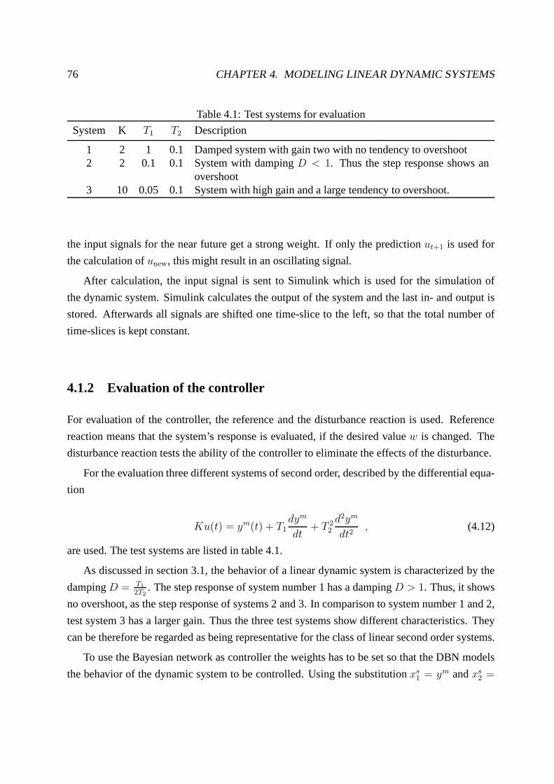
76 CHAPTER 4. MODELING LINEAR DYNAMIC SYSTEMS
Table 4.1: Test systems for evaluation
System K T1 T2 Description
1 2 1 0.1 Damped system with gain two with no tendency to overshoot2 2 0.1 0.1 System with dampingD < 1. Thus the step response shows an
overshoot3 10 0.05 0.1 System with high gain and a large tendency to overshoot.
the input signals for the near future get a strong weight. If only the predictionut+1 is used for
the calculation ofunew, this might result in an oscillating signal.
After calculation, the input signal is sent to Simulink which is used for the simulation of
the dynamic system. Simulink calculates the output of the system and the last in- and output is
stored. Afterwards all signals are shifted one time-slice to the left, so that the total number of
time-slices is kept constant.
4.1.2 Evaluation of the controller
For evaluation of the controller, the reference and the disturbance reaction is used. Reference
reaction means that the system’s response is evaluated, if the desired valuew is changed. The
disturbance reaction tests the ability of the controller toeliminate the effects of the disturbance.
For the evaluation three different systems of second order,described by the differential equa-
tion
Ku(t) = ym(t) + T1dym
dt+ T 2
2
d2ym
dt2, (4.12)
are used. The test systems are listed in table 4.1.
As discussed in section 3.1, the behavior of a linear dynamicsystem is characterized by the
dampingD = T1
2T2. The step response of system number 1 has a dampingD > 1. Thus, it shows
no overshoot, as the step response of systems 2 and 3. In comparison to system number 1 and 2,
test system 3 has a larger gain. Thus the three test systems show different characteristics. They
can be therefore be regarded as being representative for theclass of linear second order systems.
To use the Bayesian network as controller the weights has to be set so that the DBN models
the behavior of the dynamic system to be controlled. Using the substitutionxs1 = ym andxs
2 =
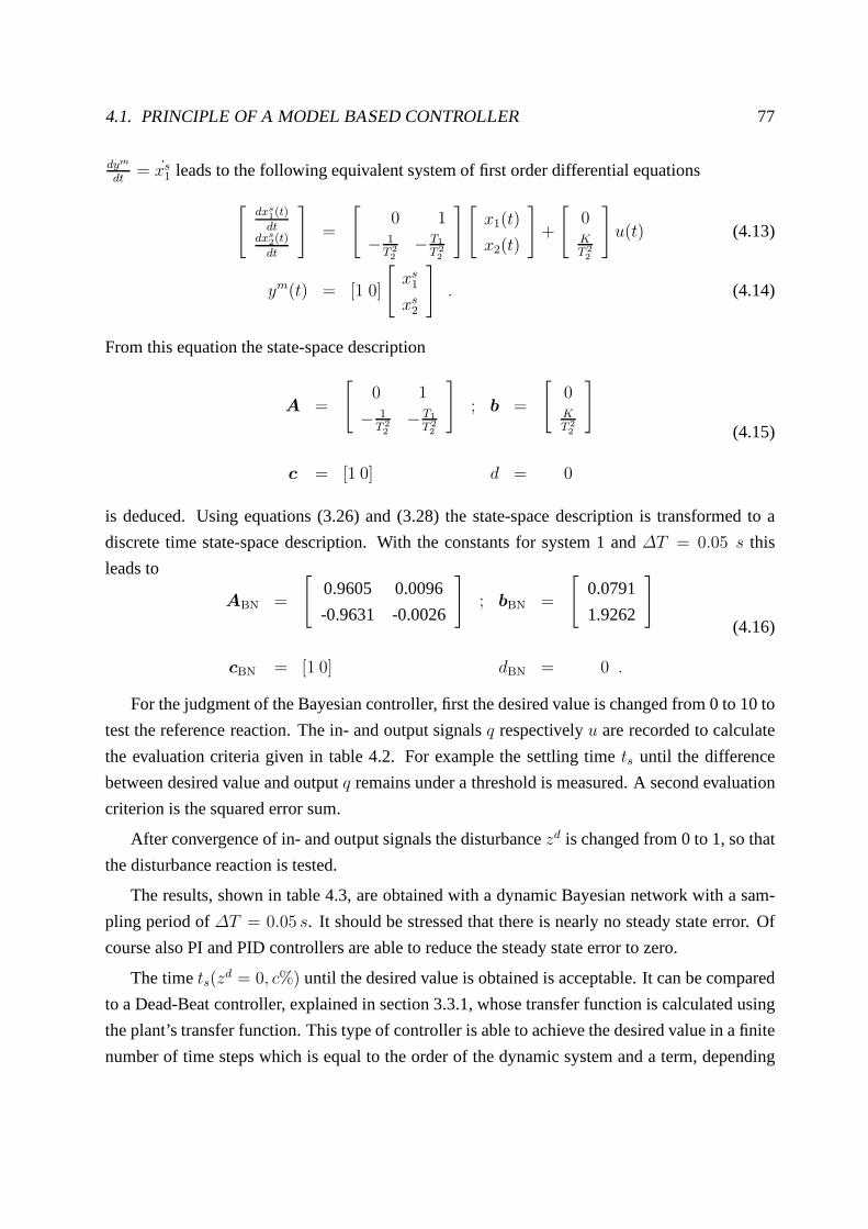
4.1. PRINCIPLE OF A MODEL BASED CONTROLLER 77
dym
dt= xs
1 leads to the following equivalent system of first order differential equations
[dxs
1(t)
dtdxs
2(t)
dt
]=
[0 1
− 1T 22− T1
T 22
][x1(t)
x2(t)
]+
[0KT 22
]u(t) (4.13)
ym(t) = [1 0]
[xs
1
xs2
]. (4.14)
From this equation the state-space description
A =
[0 1
− 1T 22− T1
T 22
]; b =
[0KT 22
]
c = [1 0] d = 0
(4.15)
is deduced. Using equations (3.26) and (3.28) the state-space description is transformed to a
discrete time state-space description. With the constantsfor system 1 and∆T = 0.05 s this
leads to
ABN =
[0.9605 0.0096
-0.9631 -0.0026
]; bBN =
[0.0791
1.9262
]
cBN = [1 0] dBN = 0 .
(4.16)
For the judgment of the Bayesian controller, first the desired value is changed from 0 to 10 to
test the reference reaction. The in- and output signalsq respectivelyu are recorded to calculate
the evaluation criteria given in table 4.2. For example the settling timets until the difference
between desired value and outputq remains under a threshold is measured. A second evaluation
criterion is the squared error sum.
After convergence of in- and output signals the disturbancezd is changed from 0 to 1, so that
the disturbance reaction is tested.
The results, shown in table 4.3, are obtained with a dynamic Bayesian network with a sam-
pling period of∆T = 0.05 s. It should be stressed that there is nearly no steady state error. Of
course also PI and PID controllers are able to reduce the steady state error to zero.
The timets(zd = 0, c%) until the desired value is obtained is acceptable. It can be compared
to a Dead-Beat controller, explained in section 3.3.1, whose transfer function is calculated using
the plant’s transfer function. This type of controller is able to achieve the desired value in a finite
number of time steps which is equal to the order of the dynamicsystem and a term, depending

78 CHAPTER 4. MODELING LINEAR DYNAMIC SYSTEMS
Table 4.2: Used evaluation criteria for controllersCriterion Description
Squared error sumId(zd) Calculated according to equation (3.64). This sum is similar to the
squared integral criterion, but is adapted to the time discrete case.Overshoot Difference between the maximal output and the desired valuee∞ Steady state error, that is the remaining error after convergence of
the output signal.ts(z
d = 0, c%) Time from changing the desired valuew until the difference be-tween the desired value and the current observed output remainssmaller thanc% of the desired value.
ts(zd = 1, c%) Same asts(zd = 0, c%), but the disturbance is changed from 0 to
1.
on the dead time of the system. For our examples a Dead-Beat controller would react in 0.1 s as
the test-systems are of second order and have no dead time.
The price for the short reaction time of the Dead-Beat controller are large input signals which
might exceed the capability of the actuators. The reaction time for the Bayesian controller can be
shortened whenunew = ut+1. Please confer with section 4.5 for a comparison between Bayesian
controller and traditional controller.
As a result of this section it is concluded that Bayesian controllers work as intended, if they
are supplied with a correct model. The next step towards a self adaptive controller is to use
training algorithms to get the weights of the Bayesian network. This will be the subject of the
next section.
4.2 Trained Bayesian controller
Before starting the discussion about the training of the Bayesian network it is necessary to clar-
ify which parameters are trained. In the preceeding sectionit was explained that a Bayesian
controller needs a special relationship between the node‘scovariances, in order to guarantee an
optimal performance of the controller. Thus, the followingparameters are excluded from the
training:
• Covariance of the input nodes. The result is that the controller reacts to a changed distur-
bance or desired value by adapting the input.
• The covariance of the nodes representing the disturbance.For our test models this value is

4.2. TRAINED BAYESIAN CONTROLLER 79
Table 4.3: Results for Bayesian controller with calculatedweights
System 1 2 3
Id(zd = 0) 8.4 9.6 10.3
e∞(zd = 0 0.02 0.01 0Overshoot 0.02 0.56 0.92Id(z
d = 1) 0.15 0.19 0.23e∞(zd = 1) 0 0 0.01ts(z
d = 0, 1%) [s] 0.45 0.45 0.7ts(z
d = 0, 3%) [s] 0.35 0.4 0.45ts(z
d = 1, 1%) [s] 0.45 0.55 0.6ts(z
d = 1, 3%) [s] 0.3 0.35 0.45
fixed to 5 for the first time-slice, for the remaining time-slicesγZd = 0.01.
• The links betweenZdt andQt get a fixed weight of one.
Excluding the parameters from training has the positive side effect that the search space is re-
stricted. This is relevant as the EM-algorithm, used for training, converges towards a local ex-
tremum.
Beside the reduction of the search space, obtained by fixing the parameter listed above, the
search space is further restricted by the usage of normal forms, discussed in section 3.1.1. The
consideration starts with the observation that the differential equation
n∑
i=0
aci
diym(t)
dti=
m∑
j=0
bcj
dju(t)
dtj(4.17)
depends on less parameters than the state-space description (confer equations (3.8) and (3.9),
discussed in section 3.1). Thus there is no unique mapping from a differential equation to the
state-space description. The usage of the observable canonical form removes this ambiguity.
When using the observable canonical formcBN is set to[0 · · · 0 1], thus only one link from the
last state node to the output is needed. The net simplifies as depicted in figure 4.3 which uses a
dynamic system of second order as example.
The dashed line fromxs1,t to xs
1,t+1 at the right hand side should indicate that this connection
is superfluous as long as only the normal form is regarded, Theexperiments in this section are
made with a net wherexs1,t andxs
1,t+1 are connected, as experiments have shown that the results

80 CHAPTER 4. MODELING LINEAR DYNAMIC SYSTEMS
utut ut+1ut+1
xs1,t+1xs
1,t+1
xs2,t+1xs
2,t+1
xs1,txs
1,t
xs2,txs
2,t
qt+1qt+1 qtqt
Figure 4.3: Simplification of a dynamic system of second order
are slightly better if a net including this edge is used.
The linkZdt → Qt is part of the representation of equation (3.10); i.e., the observed output is
obtained by adding the modeled output to the disturbance variable. Thus all links toQt are fixed,
therefore this node is excluded from training.
The next question concerns the used training signals. We used u(t) = ustepσ(t), which is
similar to the step responseσ(t), but with different step heightsustep. As second training signal
the impulse response was used. This means that
ut =
uimpulse t = 0
0 t > 0(4.18)
with uimpulse as random number. Both signals are frequently used in control theory.
For the training 40 time-series were generated using Simulink. Then the Bayesian network
is trained for 5 iterations to adapt the weights of the state nodes. Afterwards, new simulations
are started to gain fresh training signals. The procedure isrepeated 4 times so that all in all 20
iterations are made. According to our experience 20 iterations are sufficient for training. As
training algorithm the EM-algorithm is used, as this algorithm is also able to deal with hidden
variables, e.g. the state nodesXs1 andXs
2 . The experiments carried out are the same as in the last
section, first the desired value is changed from 0 to 10 to evaluate the reference reaction. After
convergence the disturbance is increased. Thus, in the firstmoment, the output signal increases
from 10 to 11. Each experiment is repeated 10 times so that also the stability of the introduced
approach can be judged.

4.2. TRAINED BAYESIAN CONTROLLER 81
Table 4.4: Results of experiments with state-space model, system 1Experiment number 1 2 3 4 5 6 7 8 9 10 Mean
Id(zd = 0) 7.46 7.43 7.45 7.61 7.37 7.69 7.67 7.63 7.51 noConv. 7.53e∞(zd = 0) 0.01 -0.01 0.01 0.00 -0.01 0.01 0.02 0.01 0.00 noConv. 0.01Overshoot 0.53 0.31 0.52 0.45 0.38 0.55 0.49 0.50 0.53 noConv. 0.48Id(zd = 1) 0.15 0.15 0.16 0.16 0.15 0.18 0.17 0.17 0.16 noConv. 0.16e∞(zd = 1) 0.03 0.02 0.03 0.04 0.02 0.04 0.05 0.04 0.03 noConv. 0.03ts(z
d = 0, 1%) [s] 0.70 0.60 0.70 0.70 0.50 0.75 0.75 0.75 0.70 noConv. 0.68ts(z
d = 0, 3%) [s] 0.50 0.35 0.45 0.50 0.40 0.55 0.55 0.55 0.50 noConv. 0.48ts(z
d = 1, 1%) [s] 0.55 0.45 0.50 0.55 0.45 0.55 0.60 0.55 0.55 noConv. 0.53ts(z
d = 1, 3%) [s] 0.30 0.30 0.30 0.35 0.30 0.35 0.35 0.35 0.35 noConv. 0.33
Table 4.5: Results of experiments with state-space model, system 2Experiment number 1 2 3 4 5 6 7 8 9 10 Mean
Id(zd = 0) 9.45 9.46 9.47 9.50 9.50 9.40 9.43 9.51 9.52 9.44 9.47e∞(zd = 0 -0.01 -0.00 -0.01 -0.01 -0.00 -0.00 -0.01 -0.01 -0.01 0.00 0.00Overshoot 0.72 1.03 0.79 0.68 1.11 1.29 0.78 0.76 0.67 0.93 0.88Id(zd = 1) 0.26 0.27 0.27 0.29 0.27 0.26 0.27 0.28 0.29 0.28 0.27e∞(zd = 1) 0.01 0.02 0.00 0.01 0.01 0.01 0.01 0.01 0.01 0.02 0.01ts(z
d = 0, 1%) [s] 0.55 0.85 0.65 0.55 0.85 0.70 0.60 0.80 0.75 0.85 0.72ts(z
d = 0, 3%) [s] 0.45 0.70 0.45 0.45 0.70 0.55 0.45 0.50 0.45 0.55 0.53ts(z
d = 1, 1%) [s] 0.70 0.75 0.75 0.85 0.70 0.75 0.70 0.80 0.90 0.85 0.78ts(z
d = 1, 3%) [s] 0.60 0.60 0.60 0.65 0.60 0.60 0.60 0.60 0.65 0.65 0.62
In general, the results for the trained Bayesian controller, listed in tables 4.4 to 4.6, are similar
to the results obtained for the analytical case. The most crucial point is the missing convergence
in the tenth case of table 4.4. Thus the mean given in the last column is taken from the first nine
cases.
The squared error sumId of the trained Bayesian controller is better than in the analytical
case. The reason for this fact gets obvious, when the input signal for the trained case is compared
with the analytical case. It becomes evident that the trained controller shows a stronger reaction
as the controller whose weights are set analytically.
The larger input signals lead to a larger overshoot of 0.48 incomparison to 0.02 in the an-
alytical case. The mean amount of the steady state error for the reference reaction is 0.01. In
the worst case – not including case 10 which shows no convergence – the steady state errore∞
is 0.02, which corresponds to 2 ‰ of the desired value. For thedisturbance reaction the steady
state error amounts to 0.05 in the worst case which is worse than the steady state error in the
reference reaction.
The results for system 2, shown in table 4.5, are slightly better than the results for system 1.

82 CHAPTER 4. MODELING LINEAR DYNAMIC SYSTEMS
0 1 2 3 4 50
2
4
6
8
10
12
Time [s]
Output
Input
In-
Ou
tpu
t
(a) Calculated weights
0 1 2 3 4 5 6 7 8−2
0
2
4
6
8
10
12
Time [s]
Output
Input
In-
Ou
tpu
t
(b) Trained weights
Figure 4.4: Signals for system 2
Particularly convergence was achieved in all cases. The established tendency, observed in the
evaluation of the first test-system, is also valid for system2. The squared error sum is slightly
smaller as in the analytical case. This is due to a larger input (Compare figures 4.4(a) and 4.4(b))
which also leads to a larger overshoot.
The mean of the steady state error is less or equal to 1‰ of the desired value for both the
reference and disturbance reaction.
The settling time is better for the inferred model, e.g. the inferred model needs 0.45 s until
the new desired value is reached, the average time for the trained model is 0.72 s.
The model for system three show the limits of the state-spaceapproach. The average steady-
state error for the third test system is 0.26, but the median of 0.02 shows that in most cases an
acceptable result is obtained.
Also the steady state error for the disturbance reaction shows that the training process is at
its limits. The average steady state error is 0.35, which is beyond 3% of the desired value. But
also for the disturbance reaction the median of approximately 0.05 is acceptable.
The settling timets(zd = 0, c%) is much larger as in the analytical case. That is due to two
cases with a remaining error larger than 1 or 3% (Confer table4.6, experiment number 3 and 4).
When these two cases are left out of the calculation the meants(zd = 0, 1%) is equal to
0.84s.

4.3. HIGHER ORDER MARKOV-MODEL 83
Table 4.6: Results of experiments with state-space model, system 3Experiment number 1 2 3 4 5 6 7 8 9 10 Mean
Id(zd = 0) 10.03 9.82 10.01 25.37 10.06 9.84 9.87 10.00 9.86 11.39 11.63e∞(zd = 0 0.03 0.01 -0.51 1.95 0.02 0.00 0.01 0.02 0.00 0.08 0.26Overshoot 1.15 0.86 1.75 7.27 1.24 0.91 1.04 1.26 1.04 0.88 1.74Id(zd = 1) 0.52 0.45 0.02 0.15 0.52 0.39 0.49 0.43 0.36 0.92 0.43e∞(zd = 1) 0.09 0.06 0.41 2.54 0.04 0.03 0.04 0.05 0.02 0.19 0.35ts(z
d = 0, 1%) [s] 1.00 0.60 4.70 18.00 1.00 0.45 0.50 0.90 0.50 1.80 2.95ts(z
d = 0, 3%) [s] 0.50 0.40 4.70 18.00 0.55 0.45 0.45 0.55 0.45 0.65 2.67ts(z
d = 1, 1%) [s] 1.85 1.40 3.70 14.05 1.30 0.95 1.25 1.00 0.85 5.50 3.19ts(z
d = 1, 3%) [s] 1.00 0.95 3.70 14.05 0.95 0.75 0.90 0.80 0.70 1.80 2.56
As summary of the experiments described in section 4.1 and 4.2 it is concluded that Bayesian
networks are a suitable mean for self-adaptive control, provided a successful training process is
given. In section 4.3 a second model based on the difference equations, introduced in section
3.1.3, is examined. This model has the great advantage of less hidden nodes. The Experiments
described in section 4.3 have shown that a higher accuracy incontrol is achieved, even if less
examples are needed for training.
4.3 Higher order Markov-model
In section 3.1.3 a second possibility for describing lineardynamic systems was introduced. In
the description by difference equation (confer equation (3.34))
ym = −n∑
i=1
aiymt−i +
n∑
i=1
biut−i (4.19)
no hidden nodes are left. Instead of using state nodes, former in- and outputsut−i andymt−i re-
spectively are taken to calculate a prediction of the next output. As in the state-space description
also the disturbance variable has to be taken into account. That is, the estimation ofzdt has to be
added toymt to figure out the observed output. This consideration leads to the model depicted in
figure 4.5 which shows a dynamic system of second order.
In comparison to the state-space model it is not possible to save the layer for the modeled
outputymt . Adding the disturbance variablezd
t to ymt directly (confer figure 4.6) leads to wrong
predictions in presence of a disturbance.
When looking at figure 4.5, particularly at nodeY mt+2, one notices that the Markov assump-
tion, explained in section 2.4, is not met asY mt+2 depends also onY m
t andUt. For models of higher
order a recourse toY mt−i andUt−i, i > 1 is necessary for the prediction ofY m
t+2. This causes prob-

84 CHAPTER 4. MODELING LINEAR DYNAMIC SYSTEMS
ut ut+1 ut+2
ymt ym
t+1 ymt+2
zdt+2zd
t+1zdt
qt+1qt qt+2
Figure 4.5: Modeling of equation (3.34) by a dynamic Bayesian network
lems, as some of the toolboxes for Bayesian networks, including the one implemented by K. P.
Murphy which is used for our experiments, are not able to dealwith Markov models of higher
order. There are two obvious solutions.
• Adding additional nodes to the model with the task to transfer the values of random vari-
ables, belonging to former time-slices, to the current one [DDN02b].
• Reimplementation of a small part of the Bayesian network toolbox. Due to the evaluation
mechanism, the unrolling of the dynamic Bayesian network, the necessary expansion of the
toolbox is restricted to the generation of the Bayesian network. The evaluation algorithm
does not need to be changed. Also the training algorithm is left untouched as it is also
based on the unchanged unrolled Bayesian network. The results obtained with this model
to control systems of second and third order are discussed insection 4.4.
The first approach, used tor the experiments in this section,has the advantage that it can be used
for rapid prototyping so that the supposition that the difference equation model is advantageous
for a Bayesian controller can be checked easily. When additional nodes are used, the same value
is represented by two different nodes in different time-slices. This leads to the structure in figure
4.7.
Of course it has to be guaranteed that the same value is assigned to nodes representing the
same value. For example the valuesut andymt are represented in the first and second time-slice in
figure 4.7. It is guaranteed by two different mechanisms thatall nodes representingut or ymt get
the same value. For input nodes the value is entered twice as evidence. For systems that show no

4.3. HIGHER ORDER MARKOV-MODEL 85
ut ut+1 ut+2
ymt ym
t+1 ymt+2
zdt+2zd
t+1zdt
Figure 4.6: Faulty model which leads to incorrect prediction
immediate reaction on changes of the input nodes, the links betweenut andymt are superfluous.
Thus, one of the input nodes is unnecessary.
For the modeled output of the system this is not possible as there is no evidence given forymt .
The solution in this case is a link between two nodes representing the same value with a fixed
weight of one. An example is the link betweenymt in the time-slice at the left and in the middle
of figure 4.7.
The next step concerns the training of the Bayesian network.Our aim using the difference
equation is to use as less hidden nodes as possible. When assuming that there is no disturbance
during training, it is possible to setzd = 0 andym = q. Thus there are no hidden nodes left.
Similar to the experiments with the state-space descriptions, some of the parameters are
clamped in order to guarantee that the controller acts as intended. The following parameters
are excluded from training:
• Variance of the input nodesγU
• Variance of the modeled outputγY m
• Both edges toQ has a fixed weight of one, the varianceγQ is set to a small value, for the
described experimentsγQ = 0.01
• The connection betweenZdt andZd
t+1 has a fixed weight of one, the variance of the first
time-slice is set to three (at the first time-slice it is not possible to make proper predictions
as the information from former signals is missing), in the remaining time-slicesγZd = 0.01.

86 CHAPTER 4. MODELING LINEAR DYNAMIC SYSTEMS
Timeslice Redundant nodes
ut−1 utut ut+1ut+1 ut+2
ymt−1 ym
tymt ym
t+1ymt+1 ym
t+2
zdt+2zd
t+1zdt
qt+1qt qt+2
Figure 4.7: Model for difference equation with redundant nodes
As there are no hidden nodes left, the number of iterations isreduced to five, but of course the
convergence of the EM-algorithm is observed immediately. The number of data sets used for
training remains 40.
The results obtained for system 1 with the difference equation model are depicted in table
4.7. The most important result is that the control signal converged in all cases; i.e., the differ-
ence equation model shows the stability necessary for real world applications. This argument is
supported by the low distortion of the training results. When table 4.4 and 4.7 are compared the
most impressive result is that the dynamic system controlled with the difference equation model
shows nearly no overshoot in comparison to an overshoot of 0.48 of the state-space model.
Table 4.7: Results of experiments with higher order Markov model, system 1Experiment number 1 2 3 4 5 6 7 8 9 10 mean
Id(zd = 0) 8.51 8.51 8.51 8.51 8.51 8.51 8.51 8.51 8.51 8.51 8.51e∞(zd = 0) -0.09 -0.09 -0.05 -0.07 -0.05 -0.10 -0.08 -0.07 -0.06 -0.06 0.07Overshoot -0.09 -0.09 -0.05 -0.07 -0.05 -0.10 -0.08 -0.07 -0.06 -0.06 -0.07Id(zd = 1) 0.11 0.11 0.11 0.11 0.11 0.11 0.11 0.11 0.11 0.11 0.11e∞(zd = 1) 0.02 0.02 0.05 0.04 0.05 0.00 0.03 0.04 0.04 0.05 0.03ts(z
d = 0, 1%) [s] 0.75 0.75 0.60 0.60 0.60 2.40 0.65 0.65 0.60 0.60 0.82ts(z
d = 0, 3%) [s] 0.45 0.45 0.40 0.40 0.40 0.45 0.40 0.40 0.40 0.40 0.42ts(z
d = 1, 1%) [s] 0.30 0.60 0.30 0.30 0.30 0.60 0.30 0.30 0.30 0.30 0.36ts(z
d = 1, 3%) [s] 0.25 0.25 0.25 0.25 0.25 0.25 0.25 0.25 0.25 0.25 0.25

4.3. HIGHER ORDER MARKOV-MODEL 87
0 1 2 3 4 5 6 70
5
10
15
20
25
30
35
40
Time [s]
Output
Input
In-
Ou
tpu
t
Figure 4.8: Signals of difference equation controller, system 1
The squared error sum for the reference reaction is better for the state-space model. The
reason for this is the same as in the comparison between the analytical and trained state-space
model. The larger overshoot results in a faster reduction ofthe difference between observed
output and desired value and therefore to a smaller squared error sum (compare figure 4.8).
For the disturbance reaction the difference equation modelshows better results, a hint that the
difference equation model is trained more accurately. Comparing the settling time shows similar
results. The state-space model is slightly better as long asthe reference reaction is compared
(0.68 s in comparison to 0.82 s of the difference equation model). If the disturbance reaction is
compared the difference equation model shows better results (0.33 s vs. 0.25 s).
Using system 2 for comparison shows similar results as system 1. Less overshoot (0.45 vs.
0.88) of the difference equation model which leads to a slightly worse squared error sumId (9.82
vs. 9.47). Despite the worse squared error sum the settling time, that is the time until the desired
value is reached, is shorter for the difference equation model.
As mentioned in section 4.2, system 3 is suited to show the limit of the state-space approach.
Comparing the results of the state-space model and the difference equation model, depicted in
tables 4.6 and 4.9, shows that the new structure clearly overcomes this limit.

88 CHAPTER 4. MODELING LINEAR DYNAMIC SYSTEMS
Table 4.8: Results of experiments with higher order Markov model, system 2Experiment number 1 2 3 4 5 6 7 8 9 10 mean
Id(zd = 0) 9.82 9.83 9.82 9.82 9.82 9.82 9.82 9.83 9.83 9.82 9.82e∞(zd = 0) 0.03 -0.03 -0.05 -0.04 -0.03 -0.05 -0.04 -0.03 -0.04 -0.04 0.04Overshoot 0.45 0.45 0.43 0.44 0.45 0.43 0.44 0.46 0.44 0.44 0.45Id(zd = 1) 0.16 0.16 0.16 0.16 0.16 0.16 0.16 0.16 0.16 0.16 0.16e∞(zd = 1) -0.04 -0.04 -0.06 -0.05 -0.04 -0.05 -0.05 -0.04 -0.05 -0.05 -0.05ts(z
d = 0, 1%) [s] 0.45 0.45 0.45 0.45 0.45 0.45 0.45 0.45 0.45 0.45 0.45ts(z
d = 0, 3%) [s] 0.40 0.40 0.40 0.40 0.40 0.40 0.40 0.40 0.40 0.40 0.40ts(z
d = 1, 1%) [s] 0.35 0.35 0.35 0.35 0.35 0.35 0.35 0.35 0.35 0.35 0.35ts(z
d = 1, 3%) [s] 0.25 0.25 0.25 0.25 0.25 0.25 0.25 0.25 0.25 0.25 0.25
Table 4.9: Results of experiments with higher order Markov model, system 3Experiment number 1 2 3 4 5 6 7 8 9 10 mean
Id(zd = 0) 9.90 9.89 9.89 10.10 9.89 9.89 9.90 9.89 9.91 9.89 9.92e∞(zd = 0) 0.01 0.01 0.01 0.03 0.01 0.01 0.01 0.01 0.01 0.01 0.01Overshoot 1.15 1.15 1.15 1.15 1.15 1.15 1.15 1.15 1.15 1.15 1.15Id(zd = 1) 0.19 0.19 0.19 0.18 0.19 0.19 0.19 0.19 0.19 0.19 0.19e∞(zd = 1) -0.04 -0.04 -0.04 0.00 -0.04 -0.04 -0.04 -0.04 -0.04 -0.04 -0.03ts(z
d = 0, 1%) [s] 0.70 0.65 0.65 1.70 0.65 0.65 0.65 0.65 0.75 0.65 0.77ts(z
d = 0, 3%) [s] 0.45 0.45 0.45 1.05 0.45 0.45 0.45 0.45 0.45 0.45 0.51ts(z
d = 1, 1%) [s] 0.60 0.60 0.60 0.55 0.60 0.60 0.60 0.60 0.60 0.60 0.60ts(z
d = 1, 3%) [s] 0.25 0.25 0.25 0.30 0.25 0.25 0.25 0.25 0.30 0.25 0.26
The results obtained with the difference equation model arein all respects better than these
obtained with the state-space model. As usual the state-space model shows the larger overshoot.
In this case this does not lead to a smaller squared error sum.The fact that the trained difference
equation model sometimes even surpasses the state space model whose weights are set, is par-
ticularly from interest. For instance the squared error sumis smaller for both, the reference and
the disturbance reaction. Also the settling times are nearly the same. The disadvantage of the
approach with redundant nodes, as depicted in figure 4.7, is the overhead for the computation of
the redundant nodes which increases linearly with the orderof the system.
4.4 Modeling of higher order systems
In sections 4.1 to 4.3 all used test systems are of second order. Even if the approach with redun-
dant nodes is still possible for higher order systems, a lot of overhead is caused by this solution.
In principle there are different possibilities to model systems with ordern > 2 which will be
discussed in this section more or less from the theoretical point of view.

4.4. MODELING OF HIGHER ORDER SYSTEMS 89
• When the state-space approach is used, it is possible to increase the number of state nodes
or the dimension of the state node to model a system of higher order.
• Splitting the system in subsystems of second order.
• Splitting of the system in parallel subsystems.
• Usage of higher order Markov models, being able to predict the output by resource to
former in- and output signals.
• Approximation of a higher order system by a system of secondorder.
When the state-space approach is used, it is theoretically also possible to model MIMO sys-
tems of higher order. But as seen in section 4.2 the training of the state-space model might cause
problems. One additional problem for systems withn > 2 is the high number of the state nodes
itself. When the junction tree of the higher order model is constructed, the state nodes and all
of their parents are all content of one clique. For a SISO system of forth order this leads to
nine-dimensional cliques, asXst−1 andUt−1 are parents of the state nodesXs
t . This leads to nu-
merical problems during inversion of the covariance matrix, included in the inference algorithm
introduced in [Lau92].
One solution of the problem is to split the system in a serial connection of second order
systems. The idea is to split the numerator and denominator of the transfer function
G(s) =N(s)
D(s)=
N1(s)
D1(s)
N2(s)
D2(s)· · · Nn/2(s)
Dn/2(s)(4.20)
into polynomialsNi(s) andDi(s) of second order. This reduces the numerical problems, but
there are two restrictions. This approach is only suitable for SISO systems, as the transfer func-
tion of MIMO systems are polynomial matrices. The other restrictions is the training which
might cause problems.
The second approach is the division in parallel subsystem. Assuming that all poles inD(s)
are real
G(s) =
p∑
k=1
(ck,1
(s− sk)+
ck,2
(s− sk)2+ · · ·+ ck,rk
(s− sk)rk
)(4.21)
wherep is the number of different poles,sk is a pole ofD(s) andrk denotes how often(s− sk)
occurs the decomposition ofG(s). ThusG(s) is decomposed in parallel subsystems, as parallel
subsystems are mapped to the sum of their transfer functions. As the number of poles is not
always known before modeling starts, this approach cannot be used in all cases.

90 CHAPTER 4. MODELING LINEAR DYNAMIC SYSTEMS
Table 4.10: Test results for system number 4
BN4
Id(zd = 0) 66.45
e∞(zd = 0) 0.05Overshoot 1.80Id(z
d = 1) 1.44e∞(zd = 1) 0.09ts(z
d = 0, 1%) [s] 7.12ts(z
d = 0, 3%) [s] 4.40ts(z
d = 1, 1%) [s] 10.92ts(z
d = 1, 3%) [s] 3.68
The most promising approach is the application of higher order Markov models. For the
evaluation of this approach the Bayesian toolbox is expanded so that Markov models of higher
order can be implemented directly without the usage of redundant nodes. For a third order system
G(s) =0.4s + 2
0.01s3 + 0.5s2 + 0.2s + 1(4.22)
whose step response shows an overshoot, the results are depicted in table 4.10. The results
are obtained with a sampling period of∆T = 0.4 s and 40 training examples. Trials with
∆T = 0.05 s fail. The reason for this might be the small number of time-slices, so that a long
term prediction is not given. For the reference reaction andthe disturbance reaction the steady
state error is below the 1% level. For a comparison with traditional controller see section 4.5.
The last possibility for modeling higher order systems is toselect a model of lower order, for
example
G(s) =K
(1 + T1s)(1 + T2s)(4.23)
might be used . Other models are introduced in [Unb97a].
4.5 Comparison to PI and Dead-Beat controller
In sections 4.1 to 4.4 the capabilities of Bayesian controllers are examined based on the criteria
listed in table 4.2. This section deals with controllers used in industrial practice in order to com-
pare their performance with the Bayesian controller (see also [DDN03b]). Due to the numerous
methods to figure out controller settings it is impossible totry out all current approaches.
We have selected the approach by Ziegler and Nichols [ZN42] which, despite its age, is

4.5. COMPARISON TO PI AND DEAD-BEAT CONTROLLER 91
Figure 4.9: Setup for experiments with PI and Dead-Beat controller
Table 4.11: Settings for PI controller
Number Kcrit tcrit ControllerD(z)
1 32.58 0.1 14.661z−6.039z−1
2 2.25 0.29 1.0125z−0.8083z−1
3 0.213 0.37 0.0959z−0.0807z−1
4 64 0.17 28.8z−19.0549z−1
one of the most commonly used approaches. When this approachis applied to digital control a
high sampling period has to be selected so that the controller operates nearly in a continuous time
space. Moreover this mechanism is originally developed foroverdamped systems, a precondition
only given for system 1.
Dead-Beat controllers are particularly designed for digital control. They guarantee that the
desired value is reached within a finite number of time steps,depending on the order of the
system and the dead time. Therefore this type of controller is suited to give a lower bound for the
settling timets. But is has to be kept in mind, that this method is based on the exact knowledge
of the transfer function and of the desired reference reaction. Particularly, the first requisite is
usually not given. For our experiments the control loop depicted in figure 4.9 is used.
To figure out the settings according to Ziegler and Nichols the controller is first used as pure
P-controller, i.e.G(z) = Kc. The controller gainKc is increased until the closed loop starts
oscillation. The controller gainKcrit and the critical timetcrit are measured. For our test sys-
tems these values are given in table 4.11. Afterwards the controller is calculated according to
table 3.1. The resulting controller is dedicated for continuous time. To adapt it to discrete time

92 CHAPTER 4. MODELING LINEAR DYNAMIC SYSTEMS
Table 4.12: Settings for Dead-Beat controller
Number Transfer functionG(z) ControllerD(z)
1 0.0791z−1+0.0188z−2
1−0.9578z−1+0.0067z−21−0.9578z−1+0.0067z−2
0.0978−0.0791z−1−0.0188z−2
2 0.2088z−1+0.1766z−2
1−1.4138z−1+0.6065z−21−1.4138z−1+0.6065z−2
0.3854−0.2088z−1−0.1766z−2
3 1.1286+1.0377z−1
1−1.5622z−1+0.7788z−2 z−1 1−1.5622z−1+0.7788z−2
2.1663−1.1286z−1−1.0377z−2
4 0.544z−1+0.0529z−2−0.0127z−3
1−1.5730z−1+0.8651z−2−2.0612e−09z−31−1.573z−1+0.8651z−2−2.0612e−09z−3
0.5842−0.544z−1−0.0529z−2+0.0127z−3
the controller setting was mapped to discrete time domain using the according matlab function.
This mapping was done using the same sampling period∆T as for the Bayesian controller to
ensure compatibility of results. But this selection is questionable as it does not guarantee the
requirement that the controller operates in nearly continuous time. For the tests, discussed in this
section, only PI-controllers are used. Tests with PID controller yield no satisfying results. Possi-
ble reasons may be the fact that the Ziegler-Nichols approach is usually restricted to overdamped
systems in continuous time domain.
For the Dead-Beat controller the dynamic system is mapped todiscrete time domain and
afterwards the controller was calculated. The results are depicted in table 4.12.
The controllers listed above are compared to a Bayesian controller, based on the difference
equation model. In difference to the results, discussed in section 4.3, the models are implemented
directly using an expansion of the BN-toolbox for higher order Markov models. Two different
settings for the Bayesian network are tested. The first version, called BNT1, uses onlyut+1 for
the calculation ofunew. That is the number of nodesk in equation (4.11) is set to 1. Hence
unew = ut+1 . (4.24)
The second version BNT4 uses four nodes for the calculation of unew, i.e
unew =1
10(4ut+1 + 3ut+2 + 2ut+3 + ut+4) . (4.25)
As figures 4.10(a) and 4.10(b) show, one of the main effects isthat the input signal is damped
down. This makes sense, because the actuator might be too slow to follow the oscillation. The

4.5. COMPARISON TO PI AND DEAD-BEAT CONTROLLER 93
Table 4.13: Test results for system number 1 and 2
Test System 1∆T = 0.05 s Test System 2∆T = 0.05 sZN DB BN1 BN4 ZN DB BN1 BN4
Id(zd = 0) 12.43 5.2 4.98 8.09 15.39 6.04 5.02 9.66
e∞(zd = 0) 0 0.01 0.03 0.06 0 0 0.01 0.02Overshoot 8.82 0.01 0.06 0.06 4.03 0 0.36 0.54Id(z
d = 1) 0.12 0.05 0.09 0.11 0.15 0.06 0.11 0.16e∞(zd = 1) 0 0.01 0.02 0.03 0 0 0.03 0.04ts(z
d = 0, 1%) [s] 1.1 0.1 0.10 0.50 3.35 0.1 0.35 0.45ts(z
d = 0, 3%) [s] 0.85 0.1 0.10 0.35 2.5 0.1 0.20 0.40ts(z
d = 1, 1%) [s] 0.55 0.1 0.15 0.55 1.5 0.1 0.15 0.30ts(z
d = 1, 3%) [s] 0.3 0.05 0.15 0.20 0.5 0.1 0.15 0.25
Table 4.14: Test results for system number 3 and 4
Test System 3∆T = 0.05 s Test System 4ZN DB BN1 BN4 ZN DB BN1 BN4
Id(zd = 0) 21.51 6.15 4.97 9.89 13.87 40.20 39.80 66.45
e∞(zd = 0) 0.01 0 0.00 0.00 0.00 0 0.03 0.05Overshoot 1.70 0 0.00 1.15 6.34 0.22 0.23 1.80Id(z
d = 1) 0.21 0.06 0.12 0.19 0.31 0.40 0.94 1.44e∞(zd = 1) 0 0 0.03 0.04 0 0 0.05 0.09ts(z
d = 0, 1%) [s] 6.05 0.1 0.05 0.65 2.65 1.2 3.88 7.12ts(z
d = 0, 3%) [s] 4.4 0.1 0.05 0.45 2.0 0.8 2.32 4.40ts(z
d = 1, 1%) [s] 2.5 0.1 0.55 0.60 1.5 0.4 5.48 10.92ts(z
d = 1, 3%) [s] 1.05 0.1 0.15 0.25 0.85 0.4 1.20 3.68
results for Ziegler Nichols are worst. Particular for system 4, the sampling period∆T has to be
decreased to 0.05 s. The other systems were tested with∆T = 0.4 s. That means that the squared
error sum in table 4.14 should not be compared to BN1, BN4, andthe Dead-Beat controller.
The comparison for system 1 shows that the Bayesian network BN1 shows similar results as
the Dead-Beat controller. For an overdamped system it mightbe sensible to select only one node
for the calculation ofunew. In this case similar settling timests are obtained. Systems two and
three both have a dampingD < 1, so that oscillation is possible. The results for BN1 and DB
are similar, but as figure 4.10(a) shows, too large input signals lead to oscillation. Also the Dead-
Beat controller shows a sudden change of the input signal at the beginning (see figure 4.11 for the
in- and output signals of the Dead-Beat controller) For the Dead-Beat controller an appropriate
mean to limit the signals of the actuator is to increase the sampling period∆T , for Bayesian

94 CHAPTER 4. MODELING LINEAR DYNAMIC SYSTEMS
0 1 2 3 4 5−60
−40
−20
0
20
40
60
Input
Output
Time [s]
In-
Ou
tpu
t
(a) BN1
0 1 2 3 4 50
2
4
6
8
10
12
Input
Output
Time [s]In
-O
utp
ut
(b) BN4
Figure 4.10: Signals of Bayesian controller, system 2, based on difference equation
0 2 4 6 8 10 12−15
−10
−5
0
5
10
15
20
25
30
Input
Output
Time [s]
In-
Ou
tpu
t
Figure 4.11: Signals of system 2 for the Dead-Beat controller

4.5. COMPARISON TO PI AND DEAD-BEAT CONTROLLER 95
networks the number of nodes used for calculation ofunew can be increased. This leads of course
to an increase of the squared error sum, as the first input signal is decreased. Additionally, the
settling time is increased.
The right hand side of table 4.14 shows that the Bayesian network approach is also suitable
for systems of third order. The steady state error is below 1%of the desired value. But the
settling time is worse than for the Dead-Beat controller.
In chapter 4 the application of Bayesian controllers to linear systems has been discussed.
The next chapter discusses the modeling of non-linearitieswith Bayesian networks. In some
books about non-linear control, some frequently occurringfunctions are listed. The idea is to
design models for these elements which can be combined to more complex models and have
the advantage, that a lot of a-priori knowledge can be used for the design. Thus some of the
parameters can be clamped, so that the training effort is reduced.
It is hard to compare the different methods. The Bayesian controller has a high time-complexity.
According to [Lau92] the “most complex operation is the weakmarginalization over a given
clique. If the clique contains discrete variablesX ∈ ∆G with state space of cardinalitynX
and q continuous variables, then the computational complexity is of the order of magnitude
q3∏
X∈GnX”.
In this chapter only continuous nodes are used, thus an upperlimit of the time complexity
is q3. The largest clique of the state-space description contains 2n state nodes plus the input
nodes (remember that at least one clique must contain the state nodes and its parents). The time
complexity ofq3 results from matrix inversion, hence it makes no differencethat only strong
marginalization is applied during inference.
The training time of a state-space model with 25 nodes is approximately 1600 s, the evalua-
tion time 0.43 s. Thus the run-time is the weak point of the Bayesian network. Its advantage is
the ability to adapt itself to different systems.
In contrary to the Bayesian controller the Dead Beat controller is based on a mathematical
description. If this description is available or can be estimated, the Dead-Beat controller is a good
choice, because it guarantees a minimal settling time and the control signals are easily calculated.
The approach of Ziegler and Nichols is restricted to overdamped systems. Additionally, it is
originally developed for continuous time systems. Thus it is a very valuable empirical formula,
but far from optimal.
So the Bayesian controller is recommended if the system is unknown, In the other case the
Dead-Beat controller offers better features. But the reader should keep in mind that the Bayesian
controller is in a prototypical stage (compare chapter 9). Moreover the comparison of this chapter

96 CHAPTER 4. MODELING LINEAR DYNAMIC SYSTEMS
is incomplete as other self-adaptive methods are not regarded.

Chapter 5
Bayesian networks for modeling nonlinear
dynamic systems
This section discusses the approximation of a nonlinear function by piecewise linear approxima-
tion. In a first approach, introduced in section “Linear Approximation”, it is shown how a hybrid
Bayesian network simulates several Taylor series at the same time.
All input variables that have a nonlinear influence on the output are represented both by a
discrete and a continuous variable. The discrete variable selects a pointua closest to the current
input u. In first models an extra nodeEQ is used that calculates the quantization erroreQ =
u−ua. This model is used without modifications for the modeling ofcalibration in hydroforming.
In section “Simplification of linear approximation” it is shown how this node is saved. This
simplified version is used for the model of saturation.
In Section 5.2 the approximation of a nonlinear function by several Taylor series is combined
with the modeling of dynamic systems. Additionally the results of section 8 are applied to restrict
the run-time.
5.1 Prototypical modeling of nonlinear units
Linear Approximation
A differentiable functionf is approximated by a Taylor series
f(u) = f(ua) + f ′(ua)(u− ua), (5.1)
97

98 CHAPTER 5. BNS FOR MODELING NONLINEAR SYSTEMS
at a pointua. The functionf denotes the approximation off , f ′ the first derivative andua an
arbitrary point.
To model the approximation of a functionf with several Taylor series the model depicted in
figure 5.1 is used. The mean off(U)’s distribution, representingf(u),
αf(U) + βf(U)eQ = f(u) (5.2)
is equal to the approximation of the functionf , provided that the mean
αf(U) = f(ua) , (5.3)
and the weight
βf(U) = −f ′(ua) (5.4)
is equal to the first derivative off at pointua. The nodeEQ calculates the difference between
the inputu and its closest pointua. This is easily obtained by setting the mean ofEQ
αEQ= ua (5.5)
and the weightβEQbetween nodeU andEQ
βEQ= −1 . (5.6)
It remains to show how to select the correct pointsua. Usually a link points from the cause to
the effect of an event, so that a linkU → Ud would be naturally. The introduction of such a link
contradicts the assumption that there are no continuous parents of discrete nodes. For exceptions
see [Mur99; LSK01].
Our experiments have shown that triggering ofUd also works with a linkUd → U . To
understand how the continuous node triggers the discrete node assume thatu is closest toua.
Thus the amount|ua − u| < |ui − u|, a 6= i. Therefore the probability distribution of nodeU is
maximal ifUd = a which leads to an increased probability ofUd = a. The increased probability
for Ud = a is used to select the corresponding parameters for the node representingf(u).
In order to obtain acceptable training results the following two conditions have to be met.
• The selected pointsu1, u2, · · · , uk (k equal to the number of states ofUd) should be near
the centers of the straight lines used to approximate the function f . This is a matter of a
good initialization.

5.1. PROTOTYPICAL MODELING OF NONLINEAR UNITS 99
f(u)
ud
u
eQ
Figure 5.1: Linear approximation by multiple Taylor series
• The standard deviations associated with the different meansui of U should be in the same
order of magnitude as the difference between two neighboredpointsui and uj. If the
scattering of the data is different for different regions ofthe functionf , the (co)variances
can be clamped or tied. At least the BN-toolbox, used for the experiments, offers these
features. For a discussion how the EM-algorithm is changed to enable clamped or tied
covariances see [Mur98a]. If the size of the regions differsseverely it is necessary to
divide some larger regions, even if they might be modeled by one line.
A critical point in training are test-plans, if one state represents only one setting, and the
second state several settings. As an example imagine a modelof the threshold process, shown in
figure 5.2.
The first state represents an inputu = 1.5, the second state all inputs between 2.5 and 5.5.
Assuming that each experiment is repeated 6 times, the variance for the second state is estimated
at
γ2 =1
23
(6(2.5− 4)2 + 6(3.5− 4)2 + 6(4.5− 4)2 + 6(5.5− 4)2
)= 1.304 . (5.7)
For the first state variance is zero. In our exampleγ1 = 0.0025 ≪ γ2 is used to demonstrate
the effect of two heavily different covariances. A comparison of the two Gaussian distributions
p(u|α1 = 1.5, γ1 = 0.0025) andp(u|α2 = 4, γ2 = 1.304) is shown in figure 5.3.
It can be seen that close tou = 1.5 the probability of state 1 is much larger than of state
2. Figure 5.4 (which shows the same two probability density functions) however, exhibits the
problem that the probability of state 2 is larger than for state 1 if the input is smaller than 1.25.
Thus the model will fail to make predictions for values smaller than 1.25.

100 CHAPTER 5. BNS FOR MODELING NONLINEAR SYSTEMS
1 1.5 2 2.5 3 3.5 4 4.5 5 5.50
0.5
1
1.5
2
2.5
3
3.5
4
4.5
5
u
f(u
)
Figure 5.2: Example for a threshold function
There are two possible solutions for the problems just discussed. The first is to use an ad-
ditional state with a similar variance, so that state one is responsible for small inputs, state 2
models inputs close to the threshold and state three is used for inputs beyond the threshold. An
example is the model for the calibration process, treated insection 7.1.1.
The second solution is to tie the covariances for different states, that is to change the maxi-
mization step of the EM algorithm, so thatγi = γj for different statesi 6= j.
Simplification of linear approximation
In the last section the approximation of an arbitrary function by several Taylor series is discussed.
This pattern is successfully applied to model preforming and calibration, discussed in section
7.1.1. Figure 5.1 shows that an extra nodeEQ for the quantification of the error is used. To
simplify this model the approximation of a functionf at a pointua
f(u) = f(ua) + f ′(ua)(u− ua) (5.8)
= f(ua)− f ′(ua)ua + f ′(ua)u (5.9)
is split in a constant termf(ua) − f ′(ua)ua and a second termf ′(ua)u depending onu. Setting
the offset of the output nodef(U) to
αf(U) = f(ua)− f ′(ua)ua (5.10)

5.1. PROTOTYPICAL MODELING OF NONLINEAR UNITS 101
0 2 4 6 8 100
1
2
3
4
5
6
7
8
u
p(u|α
,γ)
Figure 5.3: Two Gaussians
0 0.2 0.4 0.6 0.8 1 1.2 1.40
0.01
0.02
0.03
0.04
0.05
0.06
0.07
0.08
0.09
u
p(u|α
,γ)
Figure 5.4: Critical point
f(u)
ud u
Figure 5.5: Simplified linear approximation
and the weight to
βf(U) = f ′(ua) (5.11)
shows that a continuous node with a discrete parent is able toapproximate a functionf . The
used model is depicted in figure 5.5.
A precondition is that the statesud are triggered so that the probability of one state is usually
much higher than the probability of the remaining states. This is again achieved by setting
αU(ud = a) = ua (5.12)
the mean for nodeU close to the selected operating pointsua. The number of states ofUd is of
course equal to the number of operating points. The standarddeviation√
γU should be selected
similar to the distance between two neighbored operating points. Usually it is sufficient to select
102 CHAPTER 5. BNS FOR MODELING NONLINEAR SYSTEMS
a suitable value as initialization to start the training process. During the training process the value
for γU is improved by the EM algorithm.
Saturation
One of the nonlinearities discussed in section 3.2 is the saturationfsat that is described by equa-
tion (3.48). This function can be modeled by three straight lines. For the first one, a point
u1 < usat has to be selected which models the regionu ≤ usat. Thereforefsat(u1) = −ymmax.
The derivative in that region vanishes (f ′sat(u1) = 0) as the output does not depend on the input.
To model the second region a pointu2 obeying−usat ≤ u2 ≤ usat is selected. The slope
f ′sat(u2) = ym
max
usatis equal to the quotient of the maximal outputym
max by the inputusat. Provided
thatu2 is in the center of the regionu2 = 0, the function valuefsat(u2) = 0.
Similar tou1, a pointu3 with u3 > usat is selected withfsat(u3) = ymmax andf ′
sat(u3) = 0.
The consideration above results in the following means
αU(Ud = 1) = u1 (5.13)
αU(Ud = 2) = u2 (5.14)
αU(Ud = 3) = u3 (5.15)
for the input nodeU . These settings, abbreviated byαU = u1 u2 u3, represent the centers
of the piecewise approximation. The parameters of the output node are according to equation
(5.10)
αf(U) = −ymmax 0 ym
max . (5.16)
The weights of the output nodef(U)
βf(U) = 0 ymmax
usat0 (5.17)
contain the derivatives at different pointsui, 1 ≤ i ≤ 3.
There are only two different parameters which determine thesaturation curve, the minimal
and maximal outputymmax, andusat. For the training of the model it is assumed that all states of
the input nodeUd have the same probability. Additionally the saturation model implemented in
Simulink has as single parameter the lower and upper limit, the maximal outputymmax is therefore
equal tousat. As a consequence the weight of the output node is clamped to
βf(U) = 0 1 0 . (5.18)

5.1. PROTOTYPICAL MODELING OF NONLINEAR UNITS 103
As training input 600 examples are taken that are uniformly distributed between -12 and 12.
After the training the saturation is modeled with a maximal error of 0.10 and relative error of
2.27%. A comparison of the saturation curve with the prediction is given in figure 5.6.
−5 −4 −3 −2 −1 0 1 2 3 4 5−2
−1.5
−1
−0.5
0
0.5
1
1.5
2
Inputu
Ou
tpu
tym
Figure 5.6: Comparison of model and real signals for saturation
Hysteresis
The hysteresis curve depends not only on the inputu, but also on the sign of the first derivative.
The sign of the first derivative is calculated by
sign(u) = sign(ut+1 − ut) . (5.19)
The difference betweenut+1−ut is calculated by the Bayesian network depicted in figure 5.7(a).
The problem is to detect the sign of the differenceut+1 − ut = ∆u. Adding a discrete parent
to node∆U does not work. The usage of different offsetsα∆u is not suitable to distinguish
between different signs, because the mean depends on the weights and the evidence of the nodes
Ut+1 andUt.
The trick is to use a nodeCH with a constant evidencec > 0 and a discrete parentXsign of
nodeCH which switches between different weights ofCH (confer figure 5.7(b)).
Assume thatβCH(sign(u) = −1) = wβ[−1 1]; i.e., the nodeCH calculatesut − ut+1 given
that sign(u) = −1 and the weightwβ is set to one. The appropriate setting ofwβ is discussed

104 CHAPTER 5. BNS FOR MODELING NONLINEAR SYSTEMS
ut+1 ut
∆u
(a) Calculation of∆u
ut+1 ut
c
xsign
(b) Sign of∆u
Figure 5.7: Parts of the hysteresis model
later. Forsign(u) = 1 the weights
βCH(sign(u) = 1) = wβ[1 − 1] (5.20)
are set the other way round. Given that the evidence for nodeCH is always a positive constant
c the Bayesian network works as follows. Ifut+1 > ut the differenceut+1 − ut is positive, the
difference−ut+1 + ut is negative. Asc is positive, it is more likely thatxsign = 1.
When ut > ut+1, the difference−ut+1 + ut is positive. Thus the likelihood ofc being
positive is increased byxsign = −1. Therefore the Bayesian network depicted in figure 5.7(b) is
able to approximate the sign function. To be sure that the sign-function switches fast when the
relationship betweenut+1 andut changes, the weightswβ of the linksUt → CH andUt+1 → CH,
the variance of nodeCH and the constantc have to be selected carefully. If∆u = ut+1 − ut the
two distributions forsign(u) = ±1 are
p(∆u|sign(u) = 1) =1
2π√
γexp−(c−∆uwβ)2
2γ(5.21)
p(∆u|sign(u) = −1) =1
2π√
γexp−(c + ∆uwβ)
2
2γ(5.22)
To be sure that the probabilityP (xsign = 1) switches fast from 0 to 1 if the differenceut+1 − ut

5.1. PROTOTYPICAL MODELING OF NONLINEAR UNITS 105
changes its sign, the quotientp(∆u|sign(u) = 1)/p(∆u|sign(u) = −1) needs to be maximal.
This quotient is
p(∆u|sign(u) = 1)
p(∆u|sign(u) = −1)=
exp− (c−∆uwβ)2
2γ
exp− (c+∆uwβ)2
2γ
(5.23)
= exp2∆uwβc
γ. (5.24)
In order to maximize this quotient,wβ or c have to take on large values, the variance has to be
very small. For our experimentsγ = 0.2, wβ = 4, andc = 10.
After the sign is detected, it is easy to expand figure 5.7(b) so that the hysteresis curve is
modeled. Only one output node has to be added. Additionally,a link betweenUt+1 andXsign is
added to decide whether the current input is below or beyond the thresholduΘ (confer equation
(3.58)). ThusXsign has four states, two states are used to encode whether the current input
exceeds the thresholduΘ, two of them are used to represent the signsign(u).
Figure 5.9 shows that the Bayesian network depicted in figure5.8 is able to model the hys-
teresis curve. Note that figure 5.9 is based on a Bayesian network with calculated weights.
ut ut+1
xsign
ym
c
Figure 5.8: Bayesian model for hysteresis
The training of the Bayesian network is not successful, an example of a failed trial is shown
in figure 5.10.
It can be seen that the thresholduΘ is estimated incorrectly . The problem is that there is no
single parameter responsible for the encoding ofuΘ. The threshold is encoded by the selection

106 CHAPTER 5. BNS FOR MODELING NONLINEAR SYSTEMS
−5 −4 −3 −2 −1 0 1 2 3 4 5−4
−3
−2
−1
0
1
2
3
4
Inputu
Ou
tpu
tym
Figure 5.9: Comparison of model and real signals for hysteresis
of the four different offsets
αUt+1 = u1 u2 u3 u4 . (5.25)
Assuming thatu3 < −uΘ < u1 ≈ u4 < uΘ < u2 the threshold is determined by
−uΘ =u3 + u1
2(5.26)
and
uΘ =u2 + u4
2. (5.27)
Asu2 andu3 are only determined by the mean of the training data below (beyond )the lower(upper)
thresholduΘ,and not on the hysteresis curve, the result of the training depends heavily on the
selected training data.
5.2 Control of non-linear systems
In the last section the approach of piecewise linear approximation of nonlinear functions is dis-
cussed. Good results are obtained if the curve to be modeled can be divided in several straight
lines which are selected according to the inputu.
If the straight lines, approximating the curve, depend not solely on the input, but for instance
on a hidden state or on the sign of the first derivative of the input u, this approach is no longer
applicable. Therefore, a nonlinearity applied directly tothe input is regarded in the next section.

5.2. CONTROL OF NON-LINEAR SYSTEMS 107
−5 −4 −3 −2 −1 0 1 2 3 4 5−4
−3
−2
−1
0
1
2
3
4
input
out
Figure 5.10: Failed trial to train the network of figure 5.8
5.2.1 Expansion of difference equation model
A frequently occurring nonlinearity is saturation. Two examples are an amplifier and a valve.
If the output of an amplifier has reached the supply voltage, further increasing the input has no
effect. When a valve is completely closed, a further reduction of the flow rate is not possible.
Therefore a serial connection of saturation and a dynamic system of second order is discussed in
this section as an example to analyze the usage of hybrid dynamic Bayesian networks.
As a starting point the difference equation model (confer equation (4.19)) is combined with
the saturation model (confer figure 5.5 for the used saturation model). The resulting dynamic
Bayesian network is displayed in figure 5.11, the Simulink model in figure 5.12. The difference
equation model is used for first tests, because it provides more stable results in the linear case.
In comparison to the saturation model two changes are made, indicated in figure 5.13.
1. The nodes in the layer, denoted withud, have two states instead of three. In first trials it
is observed that a mean input is achieved when all three states have equal probabilities,
instead of one state having probability 1. Thus one of the three states is superfluous.
To save one state it is assumed that the nodes representing the observed input, denoted
by Uc, and the hidden output of the saturation unitUh are only connected by the discrete
nodeUd. That is the link betweenUc andUh is also saved, and that the hidden nodeUh
is regarded as conditionally independent fromUc given Ud. To coupleUc andUh, the
minimal and maximal output of the saturation element is assigned as means
αUc = αUh= 0 ym
max (5.28)

108 CHAPTER 5. BNS FOR MODELING NONLINEAR SYSTEMS
y
Manipulated variables
Distributionp(t)(ud, uh, uc, y, z, q, w)New manipulated variable
t− 2 t− 1 t t + 1 tmax − 3 tmax − 2 tmax − 1 tmax
qq q
z
w www
ud
uh
uc
Figure 5.11: Modeling a saturation at the input
to both nodes. To obtain a tight link, the variance ofUh is set to a low valueγUh= 0.01.
Intermediate outputs between 0 andymmax are achieved by different probabilities forUd’s
states. For example,P (ud = 2) = 0.8 would result in an output close to0.2·0+0.8·ymmax if
all other influences are neglected. The reduction of the number of states has also a positive
influence on the runtime which is proportional to2tmax instead of3tmax .
2. A link Ud,t → Ud,t+1 is added. In the control of linear systems any a-priori knowledge for
the input nodes is avoided, by setting the varianceγU to a maximal value. If there were no
links Ud,t → Ud,t+1, the probability distribution ofUd,t would have a severe influence on
the calculation of the manipulated value. By adding a linkUd,t → Ud,t+1 this influence is
reduced, as the conditional probability of the states ofUd,t+1 depends on the probability of
the previous time-slice. Therefore there are more time-slices used to estimate the desired
distribution.
In a first step a controller is used whose weights are calculated analytically. The result of a
controller with 6 nodes used for the representation of the past and 3 nodes for the future is

5.2. CONTROL OF NON-LINEAR SYSTEMS 109
Figure 5.12: Simulink model of test system
displayed in figure 5.14.
Table 5.1: Results of experiments with expansion of difference equation modelExperiment number 1
Id(zd = 0) 20.11e∞(zd = 0) -0.02Overshoot 0.26Id(zd = 1) 0.18e∞(zd = 1) -0.05ts(z
d = 0, 1%) 2.65ts(z
d = 0, 3%) 0.85ts(z
d = 1, 1%) 1.20ts(z
d = 1, 3%) 0.3Evaltime 32.11
At the beginning of the test shown in figure 5.14 (t < 2.9 s), the desired valuew is equal to
zero. The observed outputq after convergenceq is 1.26, that is the steady state errore∞ for a
desired value ofw = 0 is e∞ = 1.26. The reason is that the distribution ofUd,t does not only
depend onUc, which represents the required control signal, but also on previous probabilities
of Ud,t−1. During design, some constants, e.g. the means ofUc and Uh, and the probability
distribution ofUd,1, are selected so that the controller shows the best performance forw = 10.
At t = 2.95 s, the desired value is changed tow = 10. Figure 5.14 shows that the controller
operates as intended in this case. After a short time the desired value is reached nearly without
deviation (compare table 5.1). The maximal input of the manipulated variable is approximately
8.45 which is lower than the maximal input used for the lineardynamic system with the same
dynamic. But it is also lower than the maximal output of the saturation; i.e., the settling timets

110 CHAPTER 5. BNS FOR MODELING NONLINEAR SYSTEMS
IstwerteStellgroße
t t + 1
ud
uh
uc
Figure 5.13: Changes of links at the input
is longer than necessary. It could be shortened by a larger input.
The overshoot of the system is larger than for the linear system (compare table 4.3, system
1). The reason are the linksUd,t−1 → Ud,t which increase the sluggishness, but are necessary to
decrease the steady state error.
At t = 13.75 s the disturbancezd is changed to 1, once again the controller reacts as intended;
i.e., after0.3 s the largest part of the disturbance is eliminated and the steady state error is nearly
zero.
The training of the model is more complicated than in the linear case. In the linear case it
is assumed thatzd = 0 during training, thus no hidden nodes are left. In the nonlinear case the
evidence of the nodesUh,t is not given. The missing evidence for nodesUh,t leads to problems to
adapt the weight of the nodes representing the model outputY m. Training with a fixed variance
γUh= 0.01 0.01 fails, the controller shows no reaction when the desired value is changed.
Figures 5.15(a) and 5.15(b) shows the result of two trials totrain the controller with the
variance of the hidden input nodeγUh= 16 16 set to 16. For both trials the same set of
parameters are used.
At the beginning the desired value is set to zero. In both figures a large steady state error
is observed (compare figure 5.15(a) fort < 6 s and figure 5.15(b) fort < 9 s). Afterwards
the desired value is set to 10. In figure 5.15(a) the desired value is reached with low deviation,
figure 5.15(b) shows a complete failure of training. A comparison of these two figures shows
that the training of the difference equation model is unstable. The most probable reason is that

5.2. CONTROL OF NON-LINEAR SYSTEMS 111
0 5 10 15 20 250
2
4
6
8
10
12
Output
Input
Time [s]
In-
Ou
tpu
t
Figure 5.14: Reference and disturbance reaction of saturation model
the intended relation betweenUc andUh is not learnt correctly despite a-priori knowledge about
saturation.
The next section shows that the problems discussed in this section are overcome with an
extension of the state-space model.
5.2.2 State-space model
The model introduced in the last section shows unsatisfactory training results. The problem
consists of learning the relationship between the inputuc anduh. The latter is the estimated
output after saturation has taken place. Additionally, theperformance depends on the selected
desired valuew.
In this section it is tested how this problem is overcome witha state-space model with three
different operating points. The operating points are triggered by the inputu. As in the piecewise
approximation, discussed at the beginning of this chapter,different inputsu result in different
probabilities for the statesud. The states ofUd switch between different means and weights of
the state nodes. Switching between different weights meansthat the input matrix is changed
depending on the input, whereas the transfer matrix is not changed.
The first operating point represents the lower saturation. The weight betweenUd andXs in
that case is 0, the mean is equal to the product of the input vector bBN and the lower saturation
level. In our experiments the lower saturation was set to zero, not to−ymmax as indicated by
equation (3.48), so that the mean is also zero in that case.
The second point represents the usual operation mode, the mean ofXs is zero as in the linear
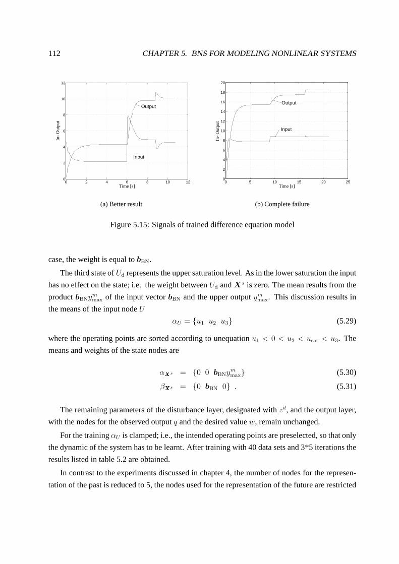
112 CHAPTER 5. BNS FOR MODELING NONLINEAR SYSTEMS
0 2 4 6 8 10 120
2
4
6
8
10
12
Input
Output
Time [s]
In-
Ou
tpu
t
(a) Better result
0 5 10 15 20 250
2
4
6
8
10
12
14
16
18
20
Input
Output
Time [s]
In-
Ou
tpu
t
(b) Complete failure
Figure 5.15: Signals of trained difference equation model
case, the weight is equal tobBN.
The third state ofUd represents the upper saturation level. As in the lower saturation the input
has no effect on the state; i.e. the weight betweenUd andXs is zero. The mean results from the
productbBNymmax of the input vectorbBN and the upper outputym
max. This discussion results in
the means of the input nodeU
αU = u1 u2 u3 (5.29)
where the operating points are sorted according to unequation u1 < 0 < u2 < usat < u3. The
means and weights of the state nodes are
αXs = 0 0 bBNymmax (5.30)
βXs = 0 bBN 0 . (5.31)
The remaining parameters of the disturbance layer, designated withzd, and the output layer,
with the nodes for the observed outputq and the desired valuew, remain unchanged.
For the trainingαU is clamped; i.e., the intended operating points are preselected, so that only
the dynamic of the system has to be learnt. After training with 40 data sets and 3*5 iterations the
results listed in table 5.2 are obtained.
In contrast to the experiments discussed in chapter 4, the number of nodes for the represen-
tation of the past is reduced to 5, the nodes used for the representation of the future are restricted

5.2. CONTROL OF NON-LINEAR SYSTEMS 113
Table 5.2: Results of experiments with state spaceExperiment number 1 2 3 mean
Id(zd = 0) 21.6964 20.7516 21.3030 21.2504e∞(zd = 0) 0.0691 -0.0426 0.0449 0.0522Overshoot 0.0894 0.0013 0.1510 0.0806Id(zd = 1) 0.1128 0.1105 0.1105 0.1113e∞(zd = 1) 0.0973 -0.0127 0.0843 0.0647ts(z
d = 0, 1%) 1.3000 1.0500 1.2500 1.2000ts(z
d = 0, 3%) 0.7000 0.7000 0.7000 0.7000ts(z
d = 1, 1%) 3.2500 0.3000 0.7000 1.4167ts(z
d = 1, 3%) 0.2000 0.2000 0.2000 0.2000Traintime 32827 29251 29345 30474Evaltime 37 38 45 40
to 2. According to the discussion in chapter 8, this has only aslight impact on the result. But
the reader should keep in mind that the experiments in chapter 8 are executed with a difference
equation model.
Table 5.2 shows that good results are obtained in all cases. Convergence is achieved in all
experiments, and the steady state errore∞ is below 1% of the desired value.
The squared error is larger than the squared error of system 1that has the same dynamic
as the test-system in this section, but no saturation at the input (For a description of system 1
see table 4.1, for the results obtained with a linear state-space system see table 4.4). The larger
squared error is due to the the connection of the discrete input nodesUd,t which is again necessary
to reduce the influence of the a-priori knowledge, but cuts the input peak (confer figure 5.17).
The settling time has increased, particularly for the reference reaction, which is partially due to
saturation. The input exceeds the upper threshold for more than half a second.
For the disturbance reaction, neither the lower nor the upper threshold are reached. Thus,
the longer settling time indicated by table 5.2 in comparison to table 4.4 is due to the Bayesian
controller. The main problem is the run-time. The evaluation time of 40 s exceeds the threshold
for real-time operation. One reason for the large run-time is that the experiments in this section
are done with the inference algorithm introduced by [LJ99] which is slower than the older one
[Lau92]. For a comparison of runtime see chapter 8. But the usage is essential as the former
inference algorithms lacks numerical stability.
The second reason is that the run-time increases exponentially with the number of time-slices
if exact inference is required.

114 CHAPTER 5. BNS FOR MODELING NONLINEAR SYSTEMS
Manipulated variables Distributionp(t)(ud, u, xs, zd, q, w)
Actual value
New manipulatedvariable
Evidence
Desired value
t− 2 t− 1 t t + 1 tmax − 1 tmax
u
zd
xs
qqq ww
· · ·
Disturbance
Fixed weight State transition xst+1 = ABNxs
t + bBNut
ud
Figure 5.16: State space approach
0 5 10 15−5
0
5
10
15
20
25
30
Time [s]
In-
Ou
tpu
t
Input
Output
Figure 5.17: Signals of state space approach

Chapter 6
Modeled manufacturing processes
The experiments in chapters 4 and 5 are done with data obtained by simulations with Simulink.
The advantages of simulations are that a large amount of datacan be collected in a controlled
environment. This is of importance particularly to test theapproach under circumstances which
are rarely observed in reality.
In this chapter modeling with Bayesian networks is applied to process data, collected by
cooperating institutes within the frame of SFB 396 (Collaborative Research Center, number 396)
“Robust shortened process sequences for lightweight sheetparts”.
The first process, hydroforming, is divided into the steps preforming, hydrocalibration, weld-
ing and trimming. The second modeled process is injection moulding which consists of the steps
preheating, handling, and injection of the plastic.
6.1 Hydroforming
6.1.1 Preforming and calibration
Preforming
During hydroforming tubes or blanks are formed by high internal pressure. At the chair of man-
ufacturing technology two blanks are formed at the same time. In a first step, both blanks are
pressed on top of each other at the flange by different clamping forces applied by a hydroform
press (see table 6.1 for a list of the parameters, measured during preforming). During the hydro-
forming process, fluid is pressed between the two blanks. As aresult, the pressure between the
blanks increases and the blanks are formed into a tool. Figures 6.1 and 6.2 show the dependency
of the pressure on the volume of the hydroforming fluid between the blanks. Both figures show
115

116 CHAPTER 6. MODELED MANUFACTURING PROCESSES
0 1 2 3 4 5 6 70
20
40
60
80
100
120
Pre
ssu
re[b
ar]
Volume [dl]
Figure 6.1: Preforming with a force of 200 kN
0 1 2 3 4 5 60
10
20
30
40
50
60
70
80
90
100
Pre
ssu
re[b
ar]
Volume [dl]
Figure 6.2: Preforming with a force of 300 kN
Table 6.1: Parameters for preforming
Variable Min Max Unit Remarks
Force 200 500 kN Increased in steps of 100 kN.Volume 0.1 7.01 dl Volume is increased, until first leaks occur.Pressure 1.04 137.35bar
the results of three experiments with equal clamping forces. With increasing pressure more and
more leaks occur, resulting in a smaller slope of the pressure. The curve progression depends
on the clamping force. Small clamping forces lead to a betterflow of material into the die, but
the process is stopped at a lower pressure due to occurring leaks. When less material is drawn
into the form, this might lead to failures during calibration, caused by lower tension. There are
two possible steps after preforming. The first possibility is that preforming is directly followed
by hydrocalibration. That means that clamping forces are increased to a maximal value, so that
the leaks are sealed. Afterwards, more hydroforming fluid ispressed between the blanks to form
the edges. The second possibility is that a welding process takes place to seal the leaks observed
at the end of preforming. In the next paragraph calibration is discussed. The welding process is
discussed later in section 6.1.3.

6.1. HYDROFORMING 117
6 7 8 9 10 11 120
20
40
60
80
100
120
140
160
180
Pre
ssu
re[b
ar]
Volume [dl]
Figure 6.3: Calibration, preforming done witha force of 200 kN
5 6 7 8 9 10 11 12 130
20
40
60
80
100
120
140
160
180
Pre
ssu
re[b
ar]
Volume [dl]
Figure 6.4: Calibration, preforming done witha force of 300 kN
Table 6.2: Parameters for calibrationVariable Min Max Unit Remarks
Force 200 500 kN During calibration the force is increased to a maximum.But the force used during preforming has an influence onthe calibration process, so the preforming forces are usedas an additional parameter for calibration.
Volume 5.33 12.12 dl Volume is increased, until the blanks burst. After burstingthe pressure drops nearly to zero.
Pressure 1.212 203.38bar
Calibration
The data to model hydrocalibration (confer table 6.2) are collected at an early phase of the “Col-
laborative Research Center”. That means calibration follows directly after preforming. In the
current version calibration is followed by laser beam welding.
No more fluid is pressed between the blanks after preforming is finished. When the press
is prepared to finish hydrocalibration in one step, the pressure drops nearly to zero, but the
hydroforming fluid remains between the blanks. Thus the initial volume for hydrocalibration is
not zero, but equal to the volume at the end of preforming (confer figures 6.3 and 6.4). A steep
increase of pressure is observed first, until the pressure atthe end of preforming is reached. Then
the slope changes, increasing the volume has a smaller effect on the pressure. The most important

118 CHAPTER 6. MODELED MANUFACTURING PROCESSES
Figure 6.5: Picture of the hydroforming tool, source LFT
point, which is of course avoided in production, is the bursting of the blanks. The bursting point
in figures 6.3 and 6.4 is situated betweenV = 10 dl andV = 11 dl. Our data are collected
during material tests, so that this effect is included in ourdata. That means that the function to be
modeled is not only non-linear, but has even a non-continuous point. The exact prediction of the
bursting-point would be helpful to increase the volume during calibration as much as possible
without risking to loose the component. A comparison between figure 6.3 and 6.4 shows that
the clamping force has an influence on the curve. Thus different models are trained for different
clamping forces used during preforming.
Modeling only one global clamping force is a simplification as four different clamping forces
effect at different points. It is the aim that the clamping forces at the flange are equal, so that the
flow of material is independent of the position. This point isdiscussed in the next section.
6.1.2 Modeling the forces of the press
Figure 6.5 shows the construction of the hydroforming tool.At the top of the tool the forces of
four different cylinders have an effect on the plate in the ram. The force of each of these cylinders
is controlled individually. The cylinders are situated at the rear, left and right hand side, and at
the front at the left and right hand side. The forces at the cylinders are therefore denoted by
Frl, Frr, Ffl, andFfr. From the plate on the top the forces act on four different pillars mounted
on three plates. Via twelve pillars the original forces affect the blank holder. The positions of

6.1. HYDROFORMING 119
Table 6.3: Parameters to model the forcesVariable Min Max Unit Remarks
Forces at cylinderFrl, Frr, Ffl, Ffr
50 400 kN There are four different cylinders whichprovide the necessary forces to press theblanks on each other. Two of them areplaced at the rear, left and right. Theother two are placed at the front.
Forces at the blank holder,FA, FC, · · · , FM
16.9 292.30 kN It is usually not possible to calculate thestandard deviation, as the experimentsare not repeated in most of the cases. Theonly exception is given in table 6.4. Thesix places of measurement are given infigure 6.5.
the twelve pillars A - N is described at the right hand side of figure 6.5. It is the aim to get equal
forcesFA, FC, · · · , FM at positions A - M to guarantee an optimal flow of material. A Bayesian
controller requires therefore knowledge about the dependency between the forces adjusted at the
top of the hydroforming press and the forces measured at the positions A, C, E, H, K, and M.
For the exploration of the dependency, 69 tests with 37 different settings are executed at the
chair of manufacturing technology. One experiment (Frl = Frr = Ffl = Ffr = 225 kN) is
repeated six times and is used to examine the dispersion of the experiments. Table 6.3 gives a
coarse overview about the test data used for examination, table 6.4 shows the dispersion of one
test.
For most of the data the results are reproducible with high accuracy. A numerical calculation
makes no sense in most of the cases, as usually the experiments are only repeated twice.
An analytical model, a neural network and a Bayesian networkare trained using the 69 data
sets . Now predictions are figured out for 14, yet un-presented, settings and compared to reality.
The results are discussed in section 7.1.2 (compare also [WBS+01]).
6.1.3 Laser beam welding
After preforming and cutting, welding takes place. Two types of joints are examined, the lap
seam joint and the lap edge joint. Several adjustments of theparameters in tables 6.5 and 6.6 are
tested to get an impression of optimal process parameters.
The laser beam is driven with a velocityv around the component. At the end a small part is

120 CHAPTER 6. MODELED MANUFACTURING PROCESSES
Table 6.4: Mean and Dispersion for the experiment withFrl = Frr = Ffl = Ffr = 225 kN
Variable/Position Standard deviation Mean
FA 2.7 kN 155.9 kNFC 11.4 kN 141.1 kNFE 0.4 kN 124.0 kNFH 5.7 kN 171.3 kNFK 3.6 kN 101.9 kNFM 0.7 kN 150.3 kN
Table 6.5: Continuous Parameters for laser-beam welding
Variable Min Max Unit Standard deviation Remarks
Defocussing -6 6 mm — Tested in steps of 2mm, when thelaser is out of focus for less then-3 mm, the quality of the joint isdecreasing.
Offset 0 6 mm —Velocity 2 7 m/min —Tensile force 0 5370 N 1460.1 Output variable, representing the
quality of the weld.
welded a second time to be sure that the component is tight after welding.
During the welding process the laser might be out of focus, inboth thex or z-axis. This
is described by the offset or defocussing of the laser beam (see figure 6.6). At the edges of
the component it is difficult to guarantee that the angle between thex-axis and the laser beam
(lap edge joint) is0 (For the lap seam joint the angle between thez-axis and the laser beam is
regarded). The tensile force is the measured output of the process and should be maximized.
When looking at the data, three parts can be distinguished. In the main part the number of
joints is kept constant, defocussing and the offset are set to zero. In this part of the data the setting
angle, the joint type and the velocity are changed. The results of these experiments are shown in
table 6.7 and figure 6.7. The result is that a velocity of approximately 4m/min is nearly optimal
for the lap edge joint.
In the second part the influence of the velocity and the numberof joints on the quality of
the joint is tested. The rest of the parameters is not changed. Table 6.8 shows the mean of 6
experiments per line. It indicates that a second joint results in a large difference of the tensile

6.1. HYDROFORMING 121
Figure 6.6: Difference between lap edge and lap seam joint, picture taken from [Kre02]
2 3 4 5 6 73600
3800
4000
4200
4400
4600
4800Lap edge joint, Angle = 0
Lap seam joint, Angle = 0
Lap edge joint, Angle =-30
Lap edge joint, Angle = 30
Ten
sile
forc
e[N
]
Velocity [m/min]
Figure 6.7: Dependency of tensile forceFon velocityv
−6 −4 −2 0 2 4 60
1000
2000
3000
4000
5000
Offset = 0.0mmOffset = 0.3mmOffset = 0.6mm
Defocussing [mm]
Ten
sile
forc
e[N
]
Figure 6.8: Tensile force depending on off-set and defocussing

122 CHAPTER 6. MODELED MANUFACTURING PROCESSES
Figure 6.9: Component produced by injection moulding
force for a velocity of 4m/min.
The third part explores the influence of the offset and defocussing. Figure 6.8 indicates that
there are two thresholds for the offset and defocussing. If these thresholds are exceeded, the
quality of the weld decreases. According to figure 6.8 the threshold for the offset is somewhere
between 0.3 and 0.6mm, the threshold for the admitted defocussing between -4 and -2 mm.
6.2 Injection moulding
At the experiments, carried out at the Institute of Polymer Technology, composite components,
consisting of a blank and plastic are insert moulded. The resulting component that is depicted in
figure 6.9 has the form of a T.
The plastic is injection-moulded around a blank, having a geometry of 249.3mm × 73.7mm
× 1.0 mm [EZ98]. At the beginning of the production process the cleaned blank is preheated.
Preheating is done first by an infrared heater, to shorten theprocess cycle, and afterwards by a
convection oven. After preheating the blank is carried automatically into the cavity. There is no
Table 6.6: Discrete Parameters for laser-beam welding
Variable Possible Values Remarks
Type of joint Lap edge joint, lap seam jointNumber of weldings 1 2 The effect on the force is only tested
for different velocities.Setting angle -30 0 +30

6.2. INJECTION MOULDING 123
Table 6.7: Force depending on type of weld, angle and velocity
Type of weld Angle Velocity [m/min] Tensile forceF [N] σF
Lap edge joint 0 2 4378 180Lap edge joint 0 3 4418 185Lap edge joint 0 4 4436 111Lap edge joint 0 5 4258 156Lap edge joint −30 2 4162 249Lap edge joint −30 4 4266 280Lap edge joint −30 5 4213 192Lap edge joint +30 2 3760 466Lap edge joint +30 4 4361 168Lap edge joint +30 5 4182 95Lap seam joint 0 4 3905 180Lap seam joint 0 5 3648 185Lap seam joint 0 6 4689 111Lap seam joint 0 7 4258 156
Table 6.8: Influence of the number of joints
Velocity Tensile force for one joint [N] σF Tensile force for two joints [N] σF
3 4380 104 4451 1164 4438 120 4657 2435 4362 135 4379 234
control whether the blank has reached the desired preheating temperatureτp. During transport
the blank cools off. This cooling process is not modeled. It is assumed that this factor is constant
due to the automatic transport.
Also the cavity is preheated, its temperature is denoted byτc. The melted plastic, whose
temperature is denoted byτm, is injected by high pressure and a constant velocityv = 10 mm/s
into the cavity. The curve of the pressure is depicted in figure 6.10. After injection the pressure
is kept constant for a short time to reduce the warpage. This pressure is called holding pressure
Ph. Note that an index “h” is used to distinguish the holding pressurePh from the probabilityP .
A list of the input parameters is given in table 6.9.
It is the aim of the production process that the resulting composite has a minimal warpage
and that the take-off tensionF , to separate the plastic from the blank, is maximal. To test the
impact of the input parameters on the quality parameters, listed in table 6.10, each input pa-

124 CHAPTER 6. MODELED MANUFACTURING PROCESSES
60 70 80 90 100 110 120−10
0
10
20
30
40
50
60
70
80
90
Pre
ssu
re[b
ar]
Time [s]
Holding pressure
Figure 6.10: Pressure used for injection
rameter is tested at five different levels. As this would result in 54 experiments, a statistical
test plan, discussed in [EZ98], is employed. In24 settings (outer experiments) all combina-
tions of τp ∈ 80, 260C, τm ∈ 260, 280C, τc ∈ 80, 120C, andPh ∈ 30, 70bar
are tested. The next 16 experiment (inner experiments) are carried out with all combinations of
τp ∈ 125, 215C, τm ∈ 265, 275C, τc ∈ 90, 110C, andPh ∈ 40, 60bar. As last ex-
periment the result for the central pointτp = 175C, τm = 270C, τc = 100C, andPh = 50 bar
is measured. According to the results in [EZ98] the preheating temperature and the holding pres-
sure have a large impact on the warpage. The take-off tensionF is mostly influenced by the
preheating temperatureτp, the melt temperatureτm and the holding pressurePh. These results
coincide with the first Bayesian models, discussed in the report of project part C1 [KN98] for
the years 96 - 98. Beside the input values, additional parameters are measured. Of course these
values are strongly correlated to the input values listed intable 6.9. So all of them have an in-
fluence on the quality parameters. A selection, according tothe correlation between the selected
parameter and the take-off tension, is made to reduce the number of models to be analyzed. The
selected values, together with a short explanation, are listed in table 6.11.
In the first period of the Collaborative Research Center onlythe input values are used in the
model. In section 7.2 it is discussed whether the additionalmeasurements listed in table 6.11 are
suited to improve the prediction of the take-off tension.

6.2. INJECTION MOULDING 125
Table 6.9: Input parameters for injection moulding
Variable Min Max Unit Remarks
Preheating temperatureτp 80 260 C Temperature of the metal. During han-dling the metal is moved from preheat-ing to the tool, and thus cooling takesplace. Five different settingsτp ∈80, 125, 170, 215, 260 are tested.
Melt temperatureτm 260 280 C Five different settings are testedfor the temperature of plasticτm ∈ 260, 265, 270, 275, 280.
Temperature of cavityτc 80 120 C Five different settings τc ∈80, 90, 100, 110, 120.
Holding pressurePh 30 70 bar PressurePh ∈ 30, 40, 50, 60, 70 whichis used for the injection of the plastic.
Velocity v 10 10 mm/s The velocity is kept constant for all exper-iments.
Table 6.10: Quality parameters for injection moulding
Variable Min Max Unit Remarks
Take-off tensionF 3130 5920 N Force needed to divide the metal from the plastic.Warpage -0.04 0.68 mm Warpage of the product.
Table 6.11: Additional measurements for injection moulding
Variable Min Max Unit Remarks
CushionC 0.4 19.1 mm Length proportional to the amountof plastic, which is not pressed inthe tool.
Plasticizing strokespl 67.4 71.0 mmMaximal cavity temperatureτc,max 88 132 C Maximal temperature of the cav-
ity.Work for injectionWinj 1960 3380 Nm Energy needed for filling the form.

126 CHAPTER 6. MODELED MANUFACTURING PROCESSES

Chapter 7
Process models
This chapter discusses the developed models for the manufacturing processes, discussed in chap-
ter 6. Most of the models use both discrete and continuous nodes to model nonlinearities. The
applied technique is discussed in section 5.1. Only the distribution of forces is modeled by a pure
linear model.
To judge the quality of the developed model the relative error
er =abs(yp − y)
abs(y), (7.1)
is used, i.e. the deviation of the predicted valueyp from the actual valuey is divided by the actual
valuey. Equation (7.1) is only applied for continuous random variablesy.
For discrete random variables, either the percentage of misclassifications is given or contin-
uous values are assigned to each discrete value. In the latter case equation (7.1) is used again.
The selected possibility is listed together with the model.If possible, the obtained relative error
er is compared to the dispersion of the data to estimate whetherthe error is due to scattering in
the data or caused by the model.
To assess a model, it is also necessary to test its ability to make predictions for yet un-
presented examples. Thus, the model is usually trained with90% of the data, the relative error
er is calculated based on the predictions for the remaining 10%of the data. This procedure is
employed to judge the models for preforming, calibration, and for the distribution of forces.
The data of the welding process can be divided into 48 blocks with equal input data within the
block. Here, the relative error is measured by training with47 blocks and figuring out predictions
for the remaining block. Using this mechanism, it is guaranteed that the Bayesian network has
never seen the example before.
127
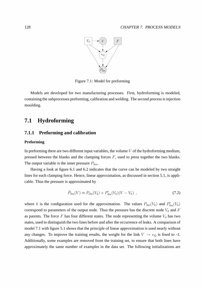
128 CHAPTER 7. PROCESS MODELS
Pihu
Vd V
eQ
F
Figure 7.1: Model for preforming
Models are developed for two manufacturing processes. First, hydroforming is modeled,
containing the subprocesses preforming, calibration and welding. The second process is injection
moulding.
7.1 Hydroforming
7.1.1 Preforming and calibration
Preforming
In preforming there are two different input variables, the volumeV of the hydroforming medium,
pressed between the blanks and the clamping forcesF , used to press together the two blanks.
The output variable is the inner pressurePihu.
Having a look at figure 6.1 and 6.2 indicates that the curve canbe modeled by two straight
lines for each clamping force. Hence, linear approximation, as discussed in section 5.1, is appli-
cable. Thus the pressure is approximated by
Pihu(V ) ≈ Pihu(Vk) + P ′ihu(Vk)(V − Vk) , (7.2)
wherek is the configuration used for the approximation. The valuesPihu(Vk) and P ′ihu(Vk)
correspond to parameters of the output node. Thus the pressure has the discrete nodeVd andF
as parents. The forceF has four different states. The node representing the volumeVd has two
states, used to distinguish the two lines before and after the occurrence of leaks. A comparison of
model 7.1 with figure 5.1 shows that the principle of linear approximation is used nearly without
any changes. To improve the training results, the weight forthe link V → eQ is fixed to -1.
Additionally, some examples are removed from the training set, to ensure that both lines have
approximately the same number of examples in the data set. The following initializations are

7.1. HYDROFORMING 129
Table 7.1: Accuracy obtained with preforming model
Variable F V Pihu
Relative Error 6.9% 4.5% 2.3%
0 1 2 3 4 5 6 70
0.2
0.4
0.6
0.8
1
1.2
1.4
Volume [dl]
Pre
ssu
re[10
2b
ar]
Figure 7.2: Preforming withF = 200 kN
0 1 2 3 4 5 60.1
0.2
0.3
0.4
0.5
0.6
0.7
0.8
0.9
1
Volume [dl]
Pre
ssu
re[10
2b
ar]
Figure 7.3: Preforming withF = 300 kN
used:
αPihu= 0.4 0.45 0.5 0.5 0.92 0.86 1 1.14 (7.3)
γPihu= 0.1 0.1 0.1 0.1 0.1 0.1 0.1 0.1 (7.4)
αeQ= 2 2 2 2 5 5 5 5 . (7.5)
The meansαPihuof the nodePihu are chosen approximately equal to the pressurePihu(Vk) at the
pointsVk. The pointsVk are defined byαeQandαV = [2 5]. The selections are obtained directly
from figures 6.1 and 6.2.
After training with the EM-algorithm (approximately 20 iterations), cross validation is exe-
cuted with the results specified in table 7.1.
For evaluation the clamping forcesF = 200 kN · · ·500 kN are assigned to the different
states ofF .
Assuming that there is an equal number of examples for all clamping forces, the mean of
the forces is 350kN. A relative error of 6.9% corresponds to an error of 24.15 kN. Moreover the
volume and the pressure are modeled with high accuracy. Figures 7.2 to 7.5 depict the prediction
of the pressure for different clamping forcesF = 200 kN · · · 500 kN. There is almost no
difference between the predictions, indicated by dotted lines and the three actual data sets (solid

130 CHAPTER 7. PROCESS MODELS
0 1 2 3 4 5 60
0.2
0.4
0.6
0.8
1
1.2
1.4
Volume [dl]
Pre
ssu
re[10
2b
ar]
Figure 7.4: Preforming withF = 400 kN
0 1 2 3 4 5 6 7 80
0.2
0.4
0.6
0.8
1
1.2
1.4
Volume [dl]
Pre
ssu
re[10
2b
ar]
Figure 7.5: Preforming withF = 500 kN
lines). The points are closer for high volumes. This is caused by the fact that not all points are
used for training to guarantee a similar number of data points before and after the occurrence
of first leaks. Similar results are obtained with variational approximation, a method which uses
continuous nodes as parents of a binary, discrete node. Thisbinary node is used to distinguish
between the two lines, before and after occurring of leaks, for each clamping force. This model
is discussed in [DDN00b], but has the drawback of slower training.
Calibration
Directly after preforming the calibration takes place1. Figures 6.3 and 6.4, which show the
relationship between the volume and the pressure, illustrate that a nonlinear curve has to be
modeled. Additionally, a non-continuous point, caused by bursting, has to be modeled (Compare
figure 6.3 atV = 10.5 dl to figure 6.4,V = 10.2 dl).
As in preforming, the technique of linear approximation is used. In comparison to preforming
the clamping forces are fixed, so thatF is no longer used as input node. But different models are
used for different clamping forces, as the result of calibration depends on the forces used during
preforming.
As a result of this consideration, the principle model of figure 5.1 can be used without any
changes. Care should be taken when selecting the number of states for nodeVd (see figure
7.6). The non-continuous point requires a small covariance. To ensure that the pressure for high
volumes is also predicted correctly, the region after bursting is modeled by two different states.1The data to be modeled are gathered in the second phase of the special research center 396. In the meantime
the preforming process is followed by the welding process. Calibration is executed after welding.

7.1. HYDROFORMING 131
Pihu
Vd
V
eQ
Figure 7.6: Model of the calibration process
One is responsible for the abrupt change, when bursting takes place, and one is used to keep the
predictions low for high volumes.
A very important point, when using a linear approximation, is the correct initialization of the
model. For example, the experiments discussed later on are carried out with 6 different states for
nodeVd and the following initializations forF = 200 kN (for each force a model with different
initializations is trained).
αV = 6.2± 0.1 6.5± 0.1 9.0± 0.1 10.0± 0.1 11.0± 0.1 11.5± 0.1 (7.6)
γV = 0+10 0+10 0+10 0+10 0+10 0+10 (7.7)
αPihu= 200± 2 100± 5 150± 5 170± 5 10± 1 10± 1 . (7.8)
The notation6.2±0.1 means that the parameter is initialized with 6.2 plus a normally distributed
(mean set to zero, standard deviation to one) random variable multiplied by 0.1.
To test the model, the data, discussed in subsection 6.1.1, is divided in a training set, con-
taining 90% of the data, and a validation set with 10% of the data. Afterwards predictions are
calculated for the validation set. The results plus the standard deviation are itemized in table 7.2.
The first impression is that the prediction of the pressure isinaccurate, which is misleading in
most of the cases. As figures 7.7 till 7.10 indicate; the dotted line, representing the prediction of
the Bayesian network, is close to the original data, depicted by a solid line.
The high error is caused by predictions close to the burstingpoint. Here, an accurate predic-
tion is nearly impossible due to scattering in the data.
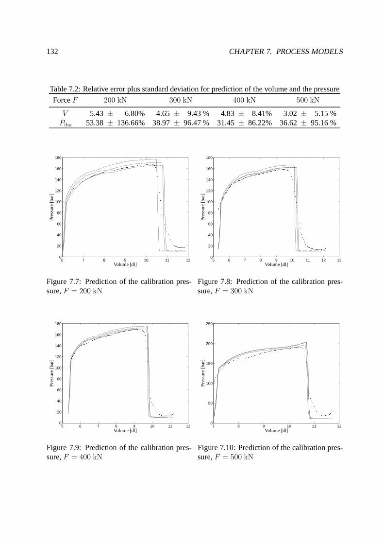
132 CHAPTER 7. PROCESS MODELS
Table 7.2: Relative error plus standard deviation for prediction of the volume and the pressure
ForceF 200 kN 300 kN 400 kN 500 kN
V 5.43 ± 6.80% 4.65± 9.43 % 4.83± 8.41% 3.02± 5.15 %Pihu 53.38 ± 136.66% 38.97± 96.47 % 31.45± 86.22% 36.62± 95.16 %
6 7 8 9 10 11 120
20
40
60
80
100
120
140
160
180
Volume [dl]
Pre
ssu
re[b
ar]
Figure 7.7: Prediction of the calibration pres-sure,F = 200 kN
5 6 7 8 9 10 11 12 130
20
40
60
80
100
120
140
160
180
Volume [dl]
Pre
ssu
re[b
ar]
Figure 7.8: Prediction of the calibration pres-sure,F = 300 kN
5 6 7 8 9 10 11 120
20
40
60
80
100
120
140
160
180
Volume [dl]
Pre
ssu
re[b
ar]
Figure 7.9: Prediction of the calibration pres-sure,F = 400 kN
7 8 9 10 11 120
50
100
150
200
250
Volume [dl]
Pre
ssu
re[b
ar]
Figure 7.10: Prediction of the calibration pres-sure,F = 500 kN

7.1. HYDROFORMING 133
Table 7.3: Control points, forces given in kN
Number Ffl Frl Frr Ffr FA FC FE FH FK FM
1 50 50 50 50 41 43 34 49 21 342 94 113 94 87 63 67 52 76 41 613 100 100 100 100 66 65 52 72 36 594 150 150 150 150 108 102 83 109 64 965 73 241 200 50 87 75 61 103 69 996 200 200 200 200 139 132 108 143 87 1267 260 262 139 193 129 150 126 173 106 1338 250 250 250 250 179 169 135 173 112 1619 300 300 300 300 216 206 165 211 139 19510 335 300 300 150 171 180 150 213 144 18211 350 350 350 350 249 237 191 242 163 22412 365 319 227 358 209 226 184 236 154 19513 392 396 305 396 237 250 201 258 173 22314 400 400 400 400 280 264 210 266 183 253
High differences between the actual values and the prediction take place for very small vol-
umes. In all cases, the predicted values are too high (compare the solid and the dotted lines in
figures 7.7 to 7.10). The reason might be a low number of data for that section of the curve. A
changed initialization is not expected to lead to an improvement, since the selected values are at
the lower end.
In the next section the distribution of the forces occurringin the press are modeled. This
process is of great importance for control.
7.1.2 Modeling the forces of the press
An important point in hydroforming, having a major influenceon the result, are the forces found
at the load cells. It is the aim to have similar or equal forcesat all points. This results in an
equal movement of the blank in the form. Then the thickness ofthe blanks remains more or less
equal which helps to avoid bursting during calibration. Therelationship between the forces at
the cylinderFrl, Frr, Ffl, Ffr and at the load cellsFA · · ·FM (compare figure 6.5) is modeled to
support the control. In a first step 69 experiments are executed to gather training data for the
Bayesian network. Afterwards, the model is used to make predictions for 14 yet un-presented
points listed in table 7.3. The results are compared with reality.
Given the forces at the load cellsFA · · ·FM, predictions for the inputsFrl, Frr, Ffl, Ffr are also
calculated. For further judgment cross-validation is applied.

134 CHAPTER 7. PROCESS MODELS
Ffl Frl Frr Ffr
FA FC FE FH FK FM
Figure 7.11: Bayesian network for modeling the forces of thehydroforming press
The used model is depicted in figure 7.11. Each cylinder forceFrl, Frr, Ffl, Ffr is connected
with each output forceFA · · ·FM. All nodes are continuous ones, that is the model is purely
linear with no hidden nodes. Thus the initialization is unimportant, the EM-algorithm used to
train the 44 parameters (4 means and dispersions for the input nodes,6×4 weights, 6 means and
dispersions for the output nodes) converges immediately. That is the EM algorithm calculates the
correct parameters in the first iteration. the second iteration is used to calculate the log-likelihood
of the model, the third iteration detects convergence.
To test the model, predictions for 14 control points are made. The relative error of the predic-
tions is listed in table 7.4 in the columnsFA · · ·FM. The result for the best and the worst position
is depicted in figures 7.12 and 7.13.
0 1 2 3 4 5 6 7 8 9 10 11 12 13 14 150
50
100
150
200
250
300
350
400
450
Fo
rce
inkN
Number of control experiment
Figure 7.12: Prediction of the used force at thecylinder at the front, left hand side (best result)
0 1 2 3 4 5 6 7 8 9 10 11 12 13 14 150
50
100
150
200
250
300
350
400
Fo
rce
inkN
Number of control experiment
Figure 7.13: Prediction of the used force at thecylinder at the rear, left hand side (worst result)
The bar at the left hand side represents the prediction of theBayesian network, the bar at
the right hand side the reality. The same experiments are also executed with neural networks

7.1. HYDROFORMING 135
Table 7.4: Relative error for control experiment
Ffl Frl Frr Ffr FA FC FE FH FK FM
5.6% 16.8% 9.7% 10.9% 4.7% 5.8% 4.9% 9.6% 5.0% 5.9%
and regression polynomials. As discussed in [WBS+01] all three techniques are well suited for
prediction of the forcesFA · · ·FM.
In contrast to regression polynomials and neural networks2, Bayesian networks are also
able to predict a required input to get a desired output. Thisis possible as Bayesian networks
model a distribution of all variables. The model itself doesnot distinguish between in and output
variables, even if in most of the cases the links are directedfrom the input to the output. To
examine, whether the trained model could also act as a controller, the six output forces measured
for the points listed in table 7.3 are entered as evidence andpredictions for the forces at the
cylindersFrl, Frr, Ffl, Ffr are calculated. The relative error of the prediction is listed in table
7.4. In comparison to the prediction of the forces at the loadcellsFA · · ·FM, the results are less
accurate. A possible reason is that there might be no unique input which leads to the desired
output. It is unlikely that the model is inadequate, as the output forces are predicted with high
accuracy. To increase the quality of control additional nodes for an occurring error might be
used, as done in the difference equation model in section 4.3. The results forFA andFH are
depicted in figures 7.14 and 7.15. The prediction of the Bayesian network is at the left hand side,
the observations at the right.
0 1 2 3 4 5 6 7 8 9 10 11 12 13 14 150
50
100
150
200
250
300
Fo
rce
inkN
Number of control experiment
Figure 7.14: Prediction for force at load cell A
0 1 2 3 4 5 6 7 8 9 10 11 12 13 14 150
50
100
150
200
250
300
Fo
rce
inkN
Number of control experiment
Figure 7.15: Prediction for force at load cell H
2The experiments concerning neural networks are done with a feedforward net, trained with backpropagation.Other topologies, e.g. Boltzmann machines or Hopfield net are also able to act as associative memory.
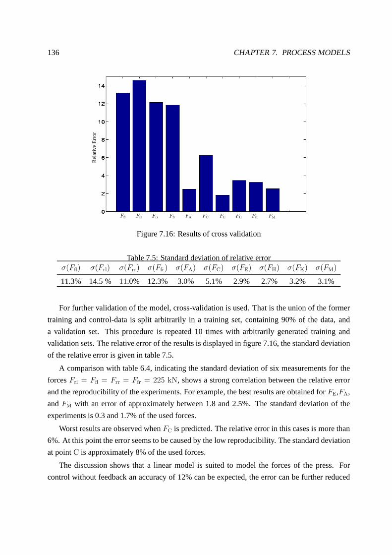
136 CHAPTER 7. PROCESS MODELS
Ffl Frl Frr Ffr FA FC FE FH FK FM
Re
lativ
eE
rro
r
Figure 7.16: Results of cross validation
Table 7.5: Standard deviation of relative errorσ(Ffl) σ(Frl) σ(Frr) σ(Ffr) σ(FA) σ(FC) σ(FE) σ(FH) σ(FK) σ(FM)
11.3% 14.5 % 11.0% 12.3% 3.0% 5.1% 2.9% 2.7% 3.2% 3.1%
For further validation of the model, cross-validation is used. That is the union of the former
training and control-data is split arbitrarily in a training set, containing 90% of the data, and
a validation set. This procedure is repeated 10 times with arbitrarily generated training and
validation sets. The relative error of the results is displayed in figure 7.16, the standard deviation
of the relative error is given in table 7.5.
A comparison with table 6.4, indicating the standard deviation of six measurements for the
forcesFrl = Ffl = Frr = Ffr = 225 kN, shows a strong correlation between the relative error
and the reproducibility of the experiments. For example, the best results are obtained forFE,FA,
andFM with an error of approximately between 1.8 and 2.5%. The standard deviation of the
experiments is 0.3 and 1.7% of the used forces.
Worst results are observed whenFC is predicted. The relative error in this cases is more than
6%. At this point the error seems to be caused by the low reproducibility. The standard deviation
at pointC is approximately 8% of the used forces.
The discussion shows that a linear model is suited to model the forces of the press. For
control without feedback an accuracy of 12% can be expected,the error can be further reduced

7.1. HYDROFORMING 137
X1X1 X2X2 X3X3
Y
Y
H1 H2 H3
Figure 7.17: Example for Bayesian network with untrainableparameters (left hand side) andmodel based on Bayesian regression
when the deviation between current and desired forces is used for further corrections.
In the next subsection a model for the welding process is discussed. The main problems to be
solved are occurring nonlinearities and the fact that not all configurations for the discrete nodes
are observed.
7.1.3 Laser beam welding
The process of laser beam welding takes place directly afterpreforming. One of its effects is that
the leaks, occurring at the end of preforming, are sealed, sothat calibration can be started. The
parameters are discussed in section 6.1.3, a good overview is given by figure 6.6.
When looking at the data three parts can be distinguished. Inthe main part the number of
joints is kept constant, defocussing and the joint-offset are set to zero. In this part of the data
the angle, the joint type (Either lap edge joint or lap seam joint), and the velocity are changed.
Additionally, some of the blanks are contaminated by hydroforming medium, and some are not.
In the second part the influence of the velocity and the numberof joints on the quality of the
joint is tested. The rest of the parameters is not changed.
In the third part the influence of defocussing and offset is tested.
It is important to map the different parts of the data also to the model. If that is not done,
this might lead to un-trainable parts of the Bayesian networks which can easily be identified.
Imagine, for example, that the influence of three binary parametersX1 · · ·X3 on a continuous
parameterY or on a binary parameterX4 is tested. The idea of the test is to keep two parameters
constant, e.g. fix their value to 1, and change the remaining parameter. This would result in a test
similar to table 7.6.
Even if all three parametersX1 · · ·X3 have an crucial impact onY , a model as shown on
the left hand side of figure 7.17 contains un-trainable parameters. The reason is that nodeY has

138 CHAPTER 7. PROCESS MODELS
Table 7.6: Example for training data
X1 X2 X3 Y
1 1 1 y1...
...1 1 1 yn
0 1 1 yn+1...
...0 1 1 y2n
1 0 1 y2n+1...
...1 0 1 y3n
1 1 0 y3n+1...
...1 1 0 y4n
three discrete parents. Thus, it has 8 different parametersfor the mean and covariance, one set of
parameters for each possible configuration. Since only 4 of them are present in the training set,
the parameter belonging to the remaining 4 configurations will remain more or less untrained.
Thus the model will show an arbitrary response when one of theun-presented configurations is
tested.
The model on the right hand side avoids this disadvantage. The effect of each variable is
trained independently. The price is that the model is unableto learn interactions between two or
more variables. Similar effects occur when the influence on adiscrete variable has to be learnt.
In this case a table with the conditional probabilitiesP(x4|x1, x2, x3) is assigned to the nodeX4.
Once again the entries for unseen configuration cannot be trained.
It should be mentioned, that the example presented above is not pathological. In product
engineering a common problem is to find out the influence of several factors on the quality
of the product. Particularly, if many factors have to be tested, it is too expensive to test all
configurations. In many cases it is reasonable to assume thatinteractions between three and more
variables have no significant influence on the result (see introductions to quality management,
e.g. [Pfe93; Mar94] ). This leads to the idea of test plans. Suppose that two settings per parameter
are sufficient for the test plan and that the engineer assumesthat the combination ofX1 · · ·X3
has no effect on the result. In this case it is possible to set aforth parameterX4 equal to the
product· of X1, X2, X3.
The product· is defined as a commutative and associative operation with+ · + = +,

7.1. HYDROFORMING 139
Table 7.7: Example for a test plan
X1 X2 X3 X4 = X1 ·X2 ·X3 Y
+ + + + y1...
...+ + + + yn
- + + - yn+1...
...- + + - y2n
+ - + - y2n+1...
...+ - + y3n
- - + + y3n+1...
...- - + + y4n
+ + - - y4n+1...
...
+ · − = −, and− · − = +. This results in the test plan outlined in table 7.7 where the
effects ofX4 andX1 · X2 · X3 cannot be distinguished. This example should reveal two main
points. First, that missing configuration might result fromwell defined test plans, and second
that according to the test plan the effect of special interactions cannot be identified and therefore
it is not worthwhile modeling them.
In the process of laser beam welding it is therefore necessary to model the influence of the
three data parts independently. In the first part the influence of the velocity, the angle and the
type of joint on the force is modeled. An F-test [Rin97] showsthat the combination of the angle
and the type of joint is significant. Thus it is necessary to combine the influence even if not all
configurations are tested. To avoid the problem of un-trainable parameters the deterministic node
H2 (confer figure 7.18), which has four different states, is introduced. Its conditional probabilities
are defined according to table 7.8 and are not changed during training. The idea is that each of
the four observed configurations is mapped to an own state ofH2. The two unobserved states, a
setting angle of plus and minus 30 together with the lap edge joint, are mapped with a probability
of 0.48 to the observation made for plus/minus 30 for the lap seam edge and with a probability
of 0.48 to the observations made for an angle of 0 together with the lap edge joint. It is not proven
that this mapping is correct, but the results are in a reasonable order of magnitude, that is a tensile
force of approximately 4000N is predicted. The influence of the velocity is not linear, as figure

140 CHAPTER 7. PROCESS MODELS
Table 7.8: Probability of nodeH2
Angle Type of joint StateH2 Probability
0 Lap edge joint 1 0.97-30 Lap edge joint 1 0.01+30 Lap edge joint 1 0.01
0 Lap seam joint 1 0.01-30 Lap seam joint 1 0.01+30 Lap seam joint 1 0.01
0 Lap edge joint 2 0.01-30 Lap edge joint 2 0.97+30 Lap edge joint 2 0.01
0 Lap seam joint 2 0.01-30 Lap seam joint 2 0.48+30 Lap seam joint 2 0.01
0 Lap edge joint 3 0.01-30 Lap edge joint 3 0.01+30 Lap edge joint 3 0.97
0 Lap seam joint 3 0.01-30 Lap seam joint 3 0.01+30 Lap seam joint 3 0.48
0 Lap edge joint 4 0.97-30 Lap edge joint 4 0.01+30 Lap edge joint 4 0.01
0 Lap seam joint 4 0.01-30 Lap seam joint 4 0.48+30 Lap seam joint 4 0.48

7.1. HYDROFORMING 141
6.7 shows. There is a maximum of the forceF , if the velocityv is approximately 4m/min. For
high velocities the weld penetration is too low, which results in a lower tensile-strength. If the
velocity is too small the weld penetration for the lap edge joint gets too high. That means that
also in this case a low tensile-strength is obtained. For a velocity of approximately 4m/min an
optimal value is reached. Hence a simple connection betweena nodev to FH1 is not sufficient.
Thus an additional node forv2 is used, so that a polynomial is used for modeling the relationship
betweenv andF .
The relationship between the number of joints and the tensile force is tested only for the lap
edge joint for a constant angle of 0. The results are shown in table 6.8.
As there is again a maximum of the tensile-strength for a velocity of about 4m/min, the
applied modeling technique is the same as for the influence ofthe angle and the type of joint.
NodeH1 is used to calculate the difference between one and two joints. The difference is added
to FH1 and assigned to nodeFH2. Assignment means that the initialization of the parameters of
nodeH1 andFH2 is done, so thatFH2 ∼ H1 + FH1. For example the initial weight vector for
FH2 is equal to[1 1].
The third part models the influence of the offset and defocussing. Regarding figure 6.8, it
turns out that this influence can be modeled more or less as a binary process. The idea is to
compare both offset and defocussing with a threshold. If theinput value, e.g. the offset, exceeds
the threshold the quality of the joint decreases dramatically. According to figure 6.8 the threshold
for the offset is somewhere between 0.3 and 0.6mm, the threshold for the admitted defocussing
between -4 and -2mm. The threshold is controlled by the two binary discrete nodes offsetd
anddefocussingd. The binary, discrete nodeH3 combines the two values. If one threshold is
exceeded, the welding might fail. This combination is realised deterministically to avoid wrong
predictions if both thresholds are exceeded.
It was mentioned that some of the parameters of the introduced model are not trained. There
are two reasons. First, the parameters of the input nodes arenot trained at all. The main reason
is that the test data are not uniformly distributed. Thus, a training of the input nodes would lead
to predictions being equal to the value mostly seen during training. Thus the prediction of values
for the input nodes would strongly depend on the selected training examples of the test plan.
Sometimes the parameters of hidden nodes are also clamped toachieve a special behavior of the
model. This helps to reduce the overall number of parameter to 44. In the following, the results
of the model are discussed.
The process of laser-beam welding is tested with 48 different configurations, whereas the
tests for each configuration are repeated six times. To test the model, training took place with 47

142 CHAPTER 7. PROCESS MODELS
Table 7.9: Relative errorOffset Defocussing Nb. of joints Velocity Angle Joint type Tensile strength
66.4% 84.6% 38.7% 22.1% 50.4% 15.5% 17.04%
configurations. Predictions are figured out for the remaining configuration.
Table 7.9 shows the relative error, but the results are sometimes misleading. To avoid division
by zero only cases with a current value not equal to zero are included.
Prediction of the tensile strengthThe classification into good and defective joints using
defocussing and offset works as intended. Only for two configurations (Offset = 0 respectively
0.3 mm, defocussing = -2mm) strong deviations are observable. The prediction of the tensile
strengthF is 2985N (3007N) instead ofF = 4876 N (4384N). The main reason is the lack
of data. To test the ability to make predictions for unknown data the tested data sets are not used
for training. As there are only three blocks with defocussing = -2 mm, two of them are used for
training. One of them leads to a proper joint, the other fails. This leads to a too low prediction.
The correct classification of the joint does not mean that an exact prediction of the force
is possible. The first reason is the great dispersion (σ = 506 N) of the data used to test the
influence of the defocussing and the offset. Together with the mean force of 2710N this results
in an unavoidable error of approximately 18%. Another source of error is that the failure of the
joint is modeled as a binary event.
Data to explore the influence of the angle, the velocity, and the number of joints are modeled
with greater accuracy. First there is less dispersion in thedata (σ = 144 N), which results in a
lower unavoidable error of 3.39% (in relation to a mean forceF = 4247 N for good joints). In
a comparative model, where defocussing and offset are disregarded, the force is modeled with a
relative error of 5.37%.
Prediction of the offsetTable 7.9 shows a relative error of 66.4% when predicting theoffset.
It should be noticed that all cases with an offset of 0mm are not part of this calculation to avoid
division by zero. In 31 of 48 blocks the tensile strength is explored for both defocussing and
offset = 0mm. The predicted offset for these cases is 0.04mm. If a Bayesian network would be
used to control laser beam welding this would not lead to a decreasing quality.
Since an offset of less than 0.3mm does not lead to a decreased quality and an offset larger
than 0.6mm results in a faulty joint (Its not possible to make a statement for the interval between
0.3 and 0.6mm as the offset was only tested for 0, 0.3 and 0.6mm), the offset can be divided
into equivalence classes. The first class includes all values between 0.0 and 0.3mm, the second
one all values larger than 0.6mm. Using these equivalence classes there are only two wrong and
7.1. HYDROFORMING 143
Table 7.10: Misclassifications, number of joints
Velocity Misclassifications Number of examples Remarks
2 3 6 No data for different angles3 7 204 2 95 3 96 0 2 No data for different angles7 1 2 No data for different angles
one questionable prediction. The first wrong prediction is made for an offset of 0.6mm and a
defocussing of -4mm. As the defocussing is a sufficient reason for a defective joint, the model
has no possibility to distinguish between different offsets. The second failure occurs for an offset
of 0.6mm and a defocussing of -2mm. In this case a value of 0.2mm is predicted which would
lead to a joint in best order. The problem might be caused by anextrapolation, as an offset of
0.6mm is an extremal value and all other examples with a defocussing of -2 mm lead to a proper
joint. For a offset of 0.6mm and a defocussing of 4.0mm an offset of 0.39mm is predicted.
There is no mean to decide whether the predicted value is in the correct equivalence class.
Prediction of defocussingFor the discussion of the result it makes sense to distinguish be-
tween two equivalence classes again. The first class contains defective joints with defocussing
of less than -4mm. The second equivalence class contains examples with a defocussing larger
than -2mm. According to these equivalence classes, there is one misclassification for an offset
of 0.6 mm and defocussing of -4mm. As the given offset is sufficient to explain the defective
joint the model has no means to distinguish the two differentequivalence classes.
A questionable prediction is made for a defocussing of -4mm and an offset of 0.3mm. In
this case a defocussing of -2.72mm is predicted. This might be a wrong prediction (it is not
possible to determine the exact position of the threshold),caused by a high force for a defective
joint.
Number of joints As already seen in table 6.8, the difference between the forces for one or
two joints is smaller than0.5σ for v = 3 or v = 5m/min. Thus, for these velocities it is nearly
impossible to distinguish between different number of joints. The results are itemized in table
7.10 which shows the number of misclassification for different velocities.
Prediction of the velocity For the node, representing the velocity, only the mean is trained.
The variance is fixed to ten which is approximately three times of the estimation. So the disper-
sion is large enough to guarantee prediction in the tested range and to avoid a strong influence of
the examples on the prediction.

144 CHAPTER 7. PROCESS MODELS
Table 7.11: Classifications of angle
Predicted angle0 -30 30
0 20 8 8Correct Angle -30 0 4 2
+30 0 1 5
Jointtyp Angle Offset
F
DefocussingNb. Joints V 2 V
H1 H2 H3
FH1
FH2
Od Dd
Figure 7.18: Model of laser beam welding
For the tested 48 blocks there are 8 cases with a prediction error larger than 1m/min. Two
of them are cases with a defective joint where the velocity has no influence on the force. Three
wrong predictions are made for lap seam joints which shows a very unregular dependency be-
tween velocity and force. For the remaining three cases the deviation is less than twom/min,
but there is no apparent reason for the deviation in these three cases.
Prediction of the angleFor the angle misclassifications can be observed in 19 of 48 blocks.
In most of the cases an angle of -30 (8 cases) or 30 (8 cases) is predicted instead of an angle
of 0. In four of these 16 misclassifications, predictions are made for a deficient joint, so that the
angle has no influence on the joint. In four other cases, predictions are made for a velocity of 6
or 7m/min, so that a lack of data might be the cause of the error. A complete overview is given
in table 7.11

7.2. INJECTION MOULDING 145
0 5 10 15 20 25 30 350
100
200
300
400
500
600
700
800
Sta
nd
ard
Dev
iatio
no
fta
ke-o
ffte
nsi
on
Block
Figure 7.19: Standard deviation of take-off tensionF
7.2 Injection moulding
In chapter 6.2 the executed test-plan is shortly discussed.Due to this test-plan only 34 configu-
ration (15 inner experiments, 16 outer experiments, one central point and two possible operating
points) are tested. Usually each setting is repeated 6 times(for some configurations outliers are
removed, so that only four or five data sets are available), the experiments for the operating points
are repeated 60 times. The standard deviation of the take-off tension is depicted in figure 7.19,
points 1-15 are taken from the inner experiments, 16 – 31 are collected executing the outer ex-
periments. The standard deviation of the operating points is given by bars 32 and 33, bar number
34 represents the standard deviation of the central point. The mean of the standard deviation is
223.2 N. In the calculation of the mean standard deviation, the values in figure 7.19 are weighted
according to the number of experiments.
From54 = 625 possible configurations only 34 are observed. A comparison with a fraction
of the test-plan for two arbitrary variables shows that evenfor a subset of two variables (compare
table 7.12) only 11 (2 combinations for the operating point has to be added) from 25 configura-
tions are observed. Thus the suggestion of subsection 7.1.3to combine only variables if all of
their configurations are observed is not applicable.
For most of the presented models in this subsection it cannotbe expected that correct pre-
dictions are made for yet un-presented combinations (compare [DN01]). The model evaluation

146 CHAPTER 7. PROCESS MODELS
Table 7.12: Fraction of executed test plan
Var1 Var2 F
2 22 44 24 41 11 55 15 53 3
τm τp Ph τc
Fd
Fc
Figure 7.20: Discrete model of injection moulding
discussed in this section is therefore done on the training-set. In section 7.2.2 a new test plan is
suggested. This test-plan restricts the number of different settings for each variable to three to
reduce the number of experiments. The second principle is touse fully factorized test plans for a
subset of the variables and to keep the rest of the variables unchanged.
7.2.1 Results
In a first experiment a model with only discrete input nodes (compare figure 7.20) is used. The
results of the experiments with this model are listed in table 7.13 (compare also [EAD+03]).
The temperature of the plastic is predicted with an relativeerror of 0.85%. In comparison to
the mean melt temperature of269.16C, this corresponds to an average deviation of2.3C, 46%
of the difference between two neighbored settings. The meanrelative error of the preheating
temperature is 11.82%, which means (τp = 171.04C) an average error of approximately20.2C.

7.2. INJECTION MOULDING 147
Table 7.13: Relative error of different models for injection moulding
Model τm τp τc Ph F Var1 Var2
Model figure 7.20 0.85% 11.82% 8.73% 12.27% 4.22%Linear model 2.31% 42.18% 14.93% 32.59% 10.25%Hybrid model figure 7.21 1.92% 40.46% 12.44% 28.45% 6.94%Work for injection 0.50% 13.57% 6.41% 7.63% 4.20% 6.79%Cushion 0.84% 11.92% 8.65% 11.82% 4.25% 57.49%Cushion and plasticizing 0.88% 11.85% 8.62% 12.00% 4.12% 57.04% 0.18%Max cavity temperature 0.87% 12.49% 12.83% 4.04% 9.43%
This is approximately 45% of the difference between two neighbored settings. The relative error
of the cavity temperature is 8.73%, comparable to approximately 8.9C (τc = 102.15C). This
error is equal to 89% of the difference between two neighbored settings. This result indicates
that the temperature of the cavity has only a minor influence on the tensile strengthF (compare
[ZE98]). The error for the prediction of the holding pressure is 12.27% or approximately 5.95
bar. This error is equal to 59% of the difference between to neighbored settings for the holding
pressure. That is all the input variables are predicted withan accuracy smaller than the difference
between two neighbored settings.
The relative error when predicting the tensile strength is 4.22%. In comparison to the mean
forceF = 3846 N , this error is approximately 162.3 N, which is smaller than the mean standard
deviation within the data blocks.
A comparison of the discrete model to the linear model (see table 7.13), shows that a linear
model is not adequate for the manufacturing process. The reason is that a manufacturing process,
considered non-linear by the engineers, cannot be modeled by a pure linear model.
Also the hybrid model, depicted in figure 7.21, shows worse results than the discrete model.
Thus the discrete model is used as base for the expansion. To enhance the prediction of the
τmd τmc τpd τpc Phd Phcτcd τcc
Fc
Figure 7.21: Hybrid model of injection moulding

148 CHAPTER 7. PROCESS MODELS
tensile strength by additional measurements several variables are available. To keep the number
of models to be tested small, a first selection is made, according to the correlation between the
tensile strength and the measurements (see table 6.11 for the selected variables). In a first attempt
the maximal cavity temperature is added. The used model is displayed in figure 7.22, the error
is reduced by 0.18%. amount of additional information is relatively small. This is only a slight
τm τp Ph τc
Fc
Fd
τc,max
Figure 7.22: Model including the influence of the feed temperature
reduction, but the reader should keep in mind that the discrete model already uses all available
input variables, so that the amount of additional information is relatively small. Additionally the
error produced by the discrete model is smaller than the standard deviation, so that a great part of
the error is due to scattering. The problem is that no predictions for un-presented data are made
for validation, so that there is a large risk that over-adaptation to the training data has happened.
When exact prediction of the input variables is required, the work needed for injection should
be added (see figure 7.23). The model including the cushion isbest for the prediction of the
preheating temperature, the model is similar to the one usedfor adding the injection work, only
the injection work is replaced by the cushion. The results intable 7.13 show that all variables
might be used to improve predictions, but the difference to the discrete model is small in most
of the cases. The main problem is that due to the test plan a large part of the parameters are
untrained. The hybrid model and the linear model might avoidthis problem. But these two
models provide the worst results; it is not tested whether these two models provide similar results
when tested with cross validation.

7.2. INJECTION MOULDING 149
τm τp Ph τc
Fc
Fd
Winj,cWinj,d
Figure 7.23: Model including the influence of the feed temperature
7.2.2 Test plan for injection moulding
The last section has revealed that the suggested models lackrobustness. A fully factorized test
plan would solve the problem, but this would severely increase the costs. To keep the experimen-
tal costs low, it is suggested to pick three variables and execute a fully factorized test plan for
those three variables. The rest of the variables is kept constant. For an example see table 7.14.
Value 2, used in this table, should be close to the operating point. Testing only three settings for
Table 7.14: Fraction of executed test plan
τp τm Ph v τc F
1 1 1 2 21 1 2 2 21 1 3 2 21 2 1 2 2...
...3 3 3 2 2
each variable is forced by cost-pressure. On the one hand picking more than three variables for a
test plan is very expensive. On the other hand it makes sense only in very rare cases as the com-
bined influence of more than three variables can be neglectedin most of the cases. Neglecting
some of the possible combinations of three variables could further reduce the cost. This type of
tests is closely related to the Bayesian network, so that thetest plan results also in valuable hints
for the structure to be used.

150 CHAPTER 7. PROCESS MODELS
Chapter 8
Real-time
A controller has to react in real-time. That is the response time is limited by the sampling period
∆T . Particularly for nonlinear models as discussed in chapter5 real-time requirement is hard to
meet. In this chapter the reduction of time-slices is discussed which is one important step toward
real-time. But further steps are necessary, e.g. the usage of approximate inference.
The run-time used for inference in a Bayesian network depends on the number of nodesnN
of the Bayesian network. For a dynamic Bayesian network, thenumber of nodesnN is a multiple
of the number of time-slicestmax, and hence it is desirable to reduce the number of time-slices.
The experiments, discussed in the previous chapters, are performed with 10 time-slices for
the representation of the past and 15 time-slices for present and future. The large number of
time-slices has an effect on the run-time as well as on the time used for training. In particular for
hybrid, dynamic Bayesian networks the time needed for inference
Tinf ≈ ntmaxs (8.1)
depends on the number of statesns per time-slice and on the number of time-slicestmax. Even if
a reduction of the number of statesns has a large effect on the run-time, this parameter is more
or less dependent on the model and on the required accuracy. Hence there seems to be no general
way to speed up the controller by reducing the number of statesns. This remark does not mean
that a reduction ofns makes no sense in special cases, for an example see section 5.2. Reducing
the number of time-slicestmax is much more promising. In the next two sections it is shown that
the number of time-slices, needed for the representation ofthe past and future, can be severely
reduced.
Another promising approach would be the usage of approximations, as discussed e.g. in
151

152 CHAPTER 8. REAL-TIME
[BK98a]. It is not discussed in this thesis.
8.1 Number of time-slices
8.1.1 Dependency on the number of nodes used for the future
The number of time-slices is an important influencing factoron the run-time of the inference
algorithm. The nodes, representing the future, have two main tasks.
First, the estimated inputsut+i are part of the calculation of the new inputunew, as described
by equation (4.11). Sometimes it makes sense to use more thanone inputut+i for the calculation
of the input to damp the control inputunew. Signals as displayed in figure 4.10(a) usually make
no sense. The reason is that the actuator is not able to followsuch high frequencies. A suitable
number of estimated input signals is application dependent. The reader should keep in mind that
there might be other methods to dampunew than the usage of additional signals for the calculation
of unew.
The second function of the future nodes is the storage of the desired valuew. It has to be
tested whether a reduction of the number of time-slices has anegative influence on the results.
Therefore the same experiments as in chapter 4 are executed.The only difference is the number
of nodesnfuture used for the representation of the future. No further reduction is possible at the
limit nfuture = 2. No evidence is given for the first time-slice of the future, as it is determined by
the past (things might be different for jump Markov systems). The second time-slice of the future
is needed to store the desired valuew. Thus it is not possible to use less than two time-slices for
the future.
The number of time-slices for the past is fixed to 10, the number of estimated signalsut+i
for the calculation ofunew is fixed to four. It is therefore possible to compare the results with the
results of chapter 4.
Additionally, to the criteria discussed in chapter 4, the time for the training and the time for
one inference step is listed. In our experiments the training is executed with 40 examples and 5
iterations of the EM-algorithm. The measurement of the evaluation-time includes the following
steps:
1. Entering all observations for in- and output to a dynamic Bayesian network withnpast +
nfuture nodes. This net contains no information about the desired value and is used for the
estimation of the disturbance.
2. Estimation of the disturbance.

8.1. NUMBER OF TIME-SLICES 153
3. Entering the lastnpast observations as the observed past and the desired value as the ob-
served value in the future. To make the estimation of input signals more robust the estima-
tion of the disturbance, obtained at step one, is used as additional evidence.
4. Estimation of signalsut+i for the calculation ofunew.
The evaluation-time thus contains all measurements necessary for the calculation of the new
signal. The measurings are done on a PC triggered with 2.4 GHz.
The results for system 2 (see table 4.1 for a definition of the test-systems and table 4.2 for
an explanation of the criteria used to evaluate the systems)are listed in table 8.1. For the experi-
ments, described by the last two columns, the number of signals used for the calculation ofunew
is reduced to two respectively one. They only show that the controller works as intended for a
low number of time-slices, e.g. the differences in the squared error sum are caused by the low
number of signalsut+i used for the calculation ofunew.
Table 8.1: Results of experiments with difference equation(system 2), 10 nodes used for the pastNumber of future nodes 13 11 9 7 5 3 2
Id(zd = 0) 9.6685 9.6741 9.6785 9.6815 9.6800 8.5862 4.9942e∞(zd = 0) 0.0205 0.0172 0.0139 0.0106 0.0071 0.0033 0.0083Overshoot 0.5405 0.5442 0.5482 0.5525 0.5584 0.1300 0.1203Id(zd = 1) 0.1500 0.1500 0.1497 0.1493 0.1493 0.1404 0.1032e∞(zd = 1) 0.0244 0.0212 0.0173 0.0130 0.0095 0.0110 0.0170ts(z
d = 0, 1%) [s] 0.4500 0.4500 0.4500 0.4500 0.4500 0.3500 0.1500ts(z
d = 0, 3%) [s] 0.4000 0.4000 0.4000 0.4000 0.4000 0.2000 0.0500ts(z
d = 1, 1%) [s] 0.3000 0.3000 0.3000 0.3000 0.3000 0.3000 0.1500ts(z
d = 1, 3%) [s] 0.2500 0.2500 0.2500 0.2500 0.2500 0.2500 0.1500Traintime [s] 279.6955 254.1279 230.0103 207.1388 181.9450 155.0763 143.4986Evaltime [s] 0.6007 0.5503 0.4942 0.4428 0.3889 0.3332 0.3051
The effect ofnfuture on the run-time and training-time is depicted in figures 8.1 and 8.2. As
the experiments are done for networks without discrete nodes, only a linear effect is observed.
For hybrid dynamic Bayesian networks with discrete nodes a larger effect is expected.
The effect on the accuracy of the controller is depicted in figures 8.3 and 8.4. The results
for nfuture < 4 are omitted as the number of nodes that are used for the calculation ofunew is
decreased in comparison to the other examples. Figure 8.3 shows the effect on the squared error
sum. At a first glance, the reduction ofnfuture seems to have a negative effect, but the effect is
only visible at the second position after decimal point.
Figure 8.4 depicts the effect of reducingnfuture on the steady state errore∞. Decreasing
nfuture has a positive effect on the steady state error. A further reduction untilnfuture = 3 has

154 CHAPTER 8. REAL-TIME
5 6 7 8 9 10 11 12 130.35
0.4
0.45
0.5
0.55
0.6
0.65
Nodes used for future
Tim
efo
rev
alu
atio
nin
sec.
Figure 8.1: Time for the generation of the new input signal
5 6 7 8 9 10 11 12 13180
190
200
210
220
230
240
250
260
270
280
Nodes used for future
Tim
efo
rtr
ain
ing
inse
c.
Figure 8.2: Time for training depending onnfuture

8.1. NUMBER OF TIME-SLICES 155
5 6 7 8 9 10 11 12 139.668
9.67
9.672
9.674
9.676
9.678
9.68
9.682
Nodes used for future
I d(z
d=
0)
Figure 8.3: Squared error sum depending on number of time-slices
5 6 7 8 9 10 11 12 130.006
0.008
0.01
0.012
0.014
0.016
0.018
0.02
0.022
e ∞(z
d=
0)
Number of nodes for future
Figure 8.4: Steady state error depending on the number of nodes for the future

156 CHAPTER 8. REAL-TIME
Table 8.2: Dependency of the accuracy on the number of nodes used for the futureNumber of future nodes 13 11 9 7 5 3 2
Id(zd = 0) 9.8833 9.8842 9.8838 9.8843 9.8829 8.9384 4.9675e∞(zd = 0) 0.0007 0.0010 0.0009 0.0005 0.0000 0.0007 0.0011Overshoot 1.1388 1.1403 1.1402 1.1406 1.1403 0.2144 0.0040Id(zd = 1) 0.1575 0.1583 0.1578 0.1556 0.1522 0.1511 0.1133e∞(zd = 1) 0.0199 0.0215 0.0190 0.0111 0.0028 0.0110 0.0185ts(z
d = 0, 1%) [s] 0.6500 0.6500 0.6500 0.6500 0.6500 0.4000 0.0500ts(z
d = 0, 3%) [s] 0.4500 0.4500 0.4500 0.4500 0.4500 0.2000 0.0500ts(z
d = 1, 1%) [s] 0.5500 0.5500 0.5500 0.8500 0.8500 0.7500 0.6500ts(z
d = 1, 3%) [s] 0.2500 0.2500 0.2500 0.2500 0.2500 0.2500 0.1500Traintime [s] 280.9525 255.7706 239.2738 281.2450 209.0050 157.5998 158.9270Evaltime [s] 0.6029 0.5502 0.5092 0.9710 0.5654 0.3379 0.3317
the same effect. Settingnfuture to the theoretical limitnfuture = 2 makes no sense, the steady
state error increases toe∞ = 0.0083. Whennfuture is set to two, there is only one node left for
encoding the desired value. As a result the information might be missing that the desired value
has to be kept constant.
Similar results are obtained for the experiments with system 3, listed in table 8.2. Also
for system 3 a reduction of the number of nodes has nearly no impact on the accuracy. As a
consequence of the discussion in this sectionnfuture is set to five, the number of signals for the
calculation ofunew is fixed to four. This setting enables a comparison between the results in this
and the following section, and chapter 4.
8.1.2 Dependency on the number of nodes used for the past
The firstnpast time-slices are used for the estimation of the past and the disturbance. Before
the experiments are discussed, the lower limit for a SISO-system from the theoretical point of
view is deduced. For the state space model, a dynamic Bayesian network to model a third order
system is depicted in figure 8.5. Note that the number of state-nodes is equal to the order of
the system. The structure is based on the assumption that thenormal form, described in section
3.1.1, is used. The reason is that normal forms are essentially for good training results.
Provided that the in- and outputs are known for all time-slices, the third stateXs3,t can be
estimated at timet based on the measurement of the outputY mt . For time-slicet + 1 the first and
the third state,Xs1,t+1 andXs
3,t+1, are assessable accurately. For the estimation of the second state
Xs2,t+1 information about the first stateXs
1,t is missing. Att + 2 enough information is available
for the estimation of all states.
For higher order systems similar considerations lead to theresult that at the first time-slice

8.1. NUMBER OF TIME-SLICES 157
Ut
Xs1,t
Xs2,t
Xs3,t
Y mt
Ut+1
Xs1,t+1
Xs2,t+1
Xs3,t+1
Y mt+1
Ut+2
Xs1,t+2
Xs2,t+2
Xs3,t+2
Y mt+2
Ut+3
Xs1,t+3
Xs2,t+3
Xs3,t+3
Y mt+3
Figure 8.5: State space model of third order
only the last state can be estimated, for the second time-slice the first and the last one. For the
estimation of all states of a system ofn-th ordern time-slices are needed.
If the structure of the DBN is based on the difference equation approach, the same result
is obtained. To figure out the minimal number of time-slices equation (3.34) is helpful. It is
necessary to have access to all signalsut−1 · · ·ut−n andymt−1 · · ·ym
t−n to make a prediction for
Y mt . That is also for the difference equationn time-slices are necessary to make exact predictions
for a system ofn-th order.
The results of the experiments with system 2 are itemized in table 8.3. The first line shows
that reducingnpast has nearly no effect on the squared error sum. The relationship between the
number of time-slices for the past and the squared error sumId(zd = 0) is displayed in figure
8.6. But a reduction also has drawbacks. The steady state error e∞(zd = 0) raises from 0.0071
to 0.0105 fornpast = 3. If the steady state-errore∞(zd = 1) for the disturbance reaction is
observed, it gets obvious that the controller is not workingproperly fornpast = 3. The steady
state error fornpast = 3 raises to 0.0347. This value is 3 to 18 times larger than the steady state
error for more time-slices. The results obtained for system3, listed in table 8.4, agree with the
results for system 2.
Reducing the number of nodes leads to nearly no changes in thesquared error sum, but to a
larger steady state error. However, a reduction tonpast = 4 seems possible, particularly when
the run-time is taken into account The results discussed so far are obtained with the inference
158 CHAPTER 8. REAL-TIME
Table 8.3: Dependency of the results on the number of nodes used for the past, system 2Number of past nodes 10 8 6 5 4 3
Id(zd = 0) 9.6800 9.6832 9.6836 9.6842 9.6861 9.7001e∞(zd = 0) 0.0071 0.0075 0.0080 0.0079 0.0084 0.0105Overshoot 0.5584 0.5578 0.5574 0.5567 0.5566 0.5523Id(zd = 1) 0.1493 0.1444 0.1426 0.1432 0.1380 0.1217e∞(zd = 1) 0.0095 0.0045 0.0022 0.0019 0.0079 0.0347ts(z
d = 0, 1%) [s] 0.4500 0.4500 0.4500 0.4500 0.4500 0.4500ts(z
d = 0, 3%) [s] 0.4000 0.4000 0.4000 0.4000 0.4000 0.4000ts(z
d = 1, 1%) [s] 0.3000 0.3000 0.5500 0.5500 0.5500 0.5500ts(z
d = 1, 3%) [s] 0.2500 0.2500 0.2500 0.2500 0.2500 0.2500Traintime [s] 181.9450 157.2597 132.0516 119.3287 106.6231 94.1040Evaltime [s] 0.3889 0.3359 0.2846 0.2557 0.2291 0.2021
Table 8.4: Dependency of the results on the number of nodes used for the past, system 3Number of past nodes 10 8 6 5 4 3
Id(zd = 0) 9.8853 9.8815 9.8792 9.8813 9.8824 9.8796e∞(zd = 0) 0.0005 0.0007 0.0024 0.0016 0.0013 0.0032Overshoot 1.1435 1.1401 1.1424 1.1439 1.1439 1.1439Id(zd = 1) 0.1556 0.1445 0.1373 0.1465 0.1481 0.1301e∞(zd = 1) 0.0111 0.0052 0.0286 0.0203 0.0163 0.0410ts(z
d = 0, 1%) [s] 0.6500 0.6500 0.6500 0.6500 0.6500 0.6500ts(z
d = 0, 3%) [s] 0.4500 0.4500 0.4500 0.4500 0.4500 0.4500ts(z
d = 1, 1%) [s] 0.8500 0.8000 0.6000 0.6000 0.6000 0.6000ts(z
d = 1, 3%) [s] 0.2500 0.2500 0.2500 0.5000 0.5000 0.5000Traintime [s] 282.0064 162.3054 136.7756 123.4775 112.0902 98.5522Evaltime [s] 0.5778 0.3556 0.2992 0.2703 0.2433 0.2142
algorithm discussed in section 2.3.2. The drawback of this algorithm are numerical instabilities
[LJ99]. It is not possible to use this algorithm for dynamic Bayesian networks with both discrete
and continuous nodes. For networks with more than 5 time-slices the result of inference is Not a
Number (NaN). As a consequence the stable algorithm, discussed in [LJ99], is examined in the
next section.
8.2 Stable Inference algorithm
The stable inference algorithm avoids switching between the moment and canonical character-
istic so that the matrix inversion in this step is avoided. Additionally the representation of a
potential is changed. In the stable algorithm the continuous nodes are divided in head and tail
nodes, the potential represents a distribution of the head nodes given the tail nodes, so that the
dimension of the covariance matrix gets smaller.

8.2. STABLE INFERENCE ALGORITHM 159
3 4 5 6 7 8 9 109.68
9.685
9.69
9.695
9.7
9.705
9.71
Number of nodes for the past
I d(z
d=
0)
Figure 8.6: Squared error sum depending on number of time-slices
In this section the measurements for system 2, withnpast = 6 andnfuture = 5 is repeated with
the new inference algorithm to get an impression whether changing the inference algorithm has
an impact on the run-time. A comparison between table 8.5 andtable 8.3 shows that the usage
of the stable inference algorithm has nearly no impact on thequality of the controller defined by
the squared error sum, overshoot and steady state error. This coincides with the expectation as
the used inference algorithm should have no impact on the calculated distribution. Comparing
Table 8.5: Runtime of the stable inference algorithmExperiment number 1 2 3 4 5 6 7 8 9 10 Mean
Id(zd = 0) 9.68 9.68 9.68 9.68 9.68 9.68 9.68 9.68 9.69 9.68 9.68e∞(zd = 0) -0.01 -0.01 -0.01 -0.01 -0.01 -0.01 -0.01 -0.01 -0.01 -0.01 0.01Overshoot 0.56 0.56 0.56 0.56 0.56 0.56 0.56 0.56 0.56 0.56 0.56Id(zd = 1) 0.14 0.15 0.14 0.14 0.14 0.14 0.14 0.14 0.14 0.14 0.14e∞(zd = 1) 0.00 0.00 0.00 0.00 0.00 0.00 0.00 0.00 0.00 0.00 0.00ts(z
d = 0, 1%) [s] 0.45 0.45 0.45 0.45 0.45 0.45 0.45 0.45 0.45 0.45 0.45ts(z
d = 0, 3%) [s] 0.40 0.40 0.40 0.40 0.40 0.40 0.40 0.40 0.40 0.40 0.40ts(z
d = 1, 1%) [s] 0.55 0.55 0.55 0.55 0.55 0.55 0.55 0.55 0.55 0.55 0.55ts(z
d = 1, 3%) [s] 0.25 0.25 0.25 0.25 0.25 0.25 0.25 0.25 0.25 0.25 0.25Traintime [s] 726 736 754 699 698 698 697 697 700 696 710Evaltime [s] 4.13 4.13 3.89 3.89 3.90 3.90 3.89 3.89 3.93 3.893.94
the time used for the training of the Bayesian network and thetime for evaluation shows that
the (current) implementation of the inference algorithm described in [LJ99] is approximately 14

160 CHAPTER 8. REAL-TIME
3 4 5 6 7 8 9 107
7.5
8
8.5
9
9.5
10
10.5
11x 10
−3
e ∞(z
d=
0)
Number of nodes for past
Figure 8.7: Steady state error depending on the number of nodes for the past
times slower (comparison of the evaluation time) than the implementation of the former algo-
rithm [Lau92]. Therefore, it is advantageous to use the former version as long as no warnings (a
warning is given e.g. when the matrix to be inverted is badly conditioned) are displayed during
runtime.

Chapter 9
Outlook and Summary
9.1 Outlook
The thesis is divided into two main parts. The first part dealswith the application of Bayesian
networks as a controller. In chapter 4 and section 5.2 preconditions and suitable models are
discussed that enable a dynamic Bayesian network to act as controller. Chapter 8 examines the
run-time and simple means for its reduction.
The second part addresses modeling of manufacturing processes like hydroforming and in-
jection moulding. In both areas large progress is achieved,yet there are still a lot of possibilities
for further optimization. Section 9.1.1 analyzes methods to improve the Bayesian controller. An
additional subject is the usage of alternative approaches to extend the possibilities of stochastic
control.
9.1.1 Usage of Bayesian networks as a controller
In this section three different aspects are discussed. First, the Bayesian controller is regarded
from the practical point of view. Problems which might occurdue to differences between simu-
lation and possible application are covered. The second paragraph deals with possible extensions
of the system so that as many systems as possible can be controlled. Finally, alternative stochastic
approaches are discussed.
Practical application The Bayesian controller is examined with simulated dynamicsystems
of second and third order. Astraining signalsthe impulse-, step-, and sine-responses (different
frequencies are used) are applied. Using a broad range of frequencies simplifies the adaptation of
the parameters. But signals collected during practical employment of the system have a different
161

162 CHAPTER 9. OUTLOOK AND SUMMARY
characteristic. Usually a controller keeps the output constant. Provided that no disturbance
occurs, the input signal is also constant. It is not possibleto learn the dynamic of the system
using constant signals. As long as only constant in- and output signals are collected, a dynamic
system can be characterized by its gain. Possible solutionsmight be to store signals which are
gathered during the occurrence of a disturbance or when the plant is started up.
A second point to be discussed is the robustness of the training process facing differences
between thestructure of the Bayesian networkand the plant to be modeled. To explore the
feasibility of Bayesian control, it was assumed that the order of the system and, as a result, the
structure of the dynamic Bayesian network is known. Structure means either the number of state
nodes or the order of the applied Markov model. To determine the order of the system several
points of view are important. Control theory offers different methods to estimate the order of
the system (see [Unb00], chapter 4.3). Some of them are applied before system identification
takes place. Additionally it might make sense to simplify the model, for example to use a model
of smaller order than the plant (see [Unb97a], chapter 9 for regularly used simplifications). The
smaller number of state nodes results in less nodes. Therefore training and evaluation time is
shortened. Assuming the equality of some time constants is another possibility to reduce the
search-space and simplify system identification.
The application of structure learning algorithms comprises some open questions. It is not
known how the special requirements of the manufacturing domain are taken into account. Partic-
ularly adding additional hidden nodes or learning a hybrid Bayesian network can be considered
as a complex problem.
Before the EM-algorithm is applied, a suitablesampling ratehas to be set. In this thesis
the sampling rate is deduced from the natural angular frequency of the system and the sampling
theorem. But this is no final solution as the formula given forthe calculation of the natural an-
gular frequency requires the knowledge of the time-constants of the system and is restricted to
systems of second order. Both conditions are usually not met. A minimization of the sampling
period does not solve the problem as it complicates the system identification and shortens the
maximal inference time (The reader should keep in mind that,in order to meet real-time require-
ments,∆T is the maximal inference time). Unbehauen suggests (confer[Unb00], section 4.4.2)
to approximate the transition function by theoretical considerations or deterministic test-signals
to figure outT63, the time when the output has reached 63% of its maximal value. A sampling
period between∆T = 1/6 T63 and∆T = 1/10 T63 is proposed.
At last therun-timehas to be discussed. In chapter 8 it is shown that run-time canbe reduced
by decreasing the number of time-slices. For hybrid Bayesian networks the number of mixture

9.1. OUTLOOK 163
components is proportional tontmaxs . That is the reduction of the number of time-slices is an
effective means to reduce run-time. But as time-measurements in chapter 5 show, solely cut-
ting down the number of time-slices is not sufficient. For discrete dynamic Bayesian networks a
possible approach is discussed in [BK98a; BK98b]. A more promising approach might be mo-
ment matching. The idea is to reduce the number of componentsby approximating a mixture of
Gaussians by a mixture of Gaussians with a lower number of mixture components. This seems
to be promising particularly for the state-space model introduced in section 5.2. In the dynamic
Bayesian model depicted in figure 5.16 the discrete nodes represent different operating points.
Usually one state is much more probable than the remaining states. When the system changes
from one operating point to the next only two states are more likely than the others. Thus it is ex-
pected that the reduction of mixture components results only in a low error. A similar principle is
applied in the modeling of possible failures within a systemof 5 tubes [KL00]. The main idea is
that the states representing none or only one error are more probable than the states representing
the occurrence of multiple errors at the same time. That means that the idea that some states are
unlikely is used to reduce the number of mixture components.
Four different problems
• Usage of real training signals.
• Identification of the structure of the system.
• Identification of the sampling rate
• Real-time inference
are discussed which might cause problems when transferringthe theoretical approach in this
thesis to a practical application. For all of them possible approaches to solve them are discussed,
therefore it is worthwhile to continue research in the domain of Bayesian control.
Improvements of the systemAs test systems only SISO systems were employed. But in
reality also a lot of MIMO systems have to be controlled. Schulz [Sch02] discusses as example
a helicopter, a hydraulic cascade, a distillation column, and a steam generator. That isMIMO
systemsare an important extension. At least the state-space approach is also used for MIMO
systems, but in reality some problems can occur. One possible source of problems is the infer-
ence algorithm. Using the inference algorithm introduced in [Lau92] might result in numerical
problems. The matrixK occurring in the canonical characteristics is initialized, so that it has
rank one (“Note thatK has rank one and is therefore typically not positive definite[Lau92]”).
But when the canonical characteristics is transformed to moment characteristics an inversion of

164 CHAPTER 9. OUTLOOK AND SUMMARY
K is required. Furthermore the calculation of marginal potentials is only guaranteed to be finite
if the according sub-matrix ofK is positive definite. Thus numerical problems are expected.
The implementation of the recent inference algorithm [LJ99] in the BN-toolbox is slower than
the implementation of the former one. Thus it is advisable touse the former algorithm as long
as it provides numerical stable results. The second problemis the training process. For the state-
space model some weights are clamped; i.e, they are excludedfrom training. As a result the
search-space is narrowed which leads to a faster and more stable training. For MIMO systems
the normal form which is used to restrict the search-space can no longer be used. Thus it has
to be checked whether the normal forms available for MIMO systems [Sch02] can be used in a
similar way.
The application of normal forms is one way of introducing a-priori knowledge into the model.
A second source of information is an analytical descriptionof the plant. But usually a complete
analytical description of the system to be controlled is notgiven. Therefore an automatic way to
include partial or qualitative [Kui94] knowledge about thesystem is needed. Possible approaches
are:
• Imprecise or incomplete knowledge might be used for a better initialization and a refined
training process. For example the weight of a linkYi → Z might be known exactly. But
in the current implementation of the BN-toolbox it is only possible to clamp a complete
weight-vector of a nodeZ. That is the weights of all linksY → Z must be known.
• Fixing a set of parameters, e.g. variance or weights of somenodes.
• When structure learning is applied a-priori knowledge might be used to include or exclude
some edges from the search process or to provide a node ordering for the learning process.
• For overdamped systems the number of nodes included in the calculation ofunew can be
reduced.
A main point of control isstability of the controlled system. For linear SISO systems good
results are obtained by using a difference equation model. But for the state-space approach the
training failed in one case, i.e. convergence was not achieved (see table 4.4). As the suggested
model for nonlinear systems are based on a state-space modela guarantee for convergence is
still of importance, particularly for the nonlinear case. Similarly a guarantee is missing that the
steady state error is reduced to zero.
Alternative approachesThere are other means for stochastic inference beside Bayesian net-
works. Well known inference algorithms are differentsamplingprocedures, e.g. Gibbs sampling.

9.1. OUTLOOK 165
Gibbs sampling is implemented for example in BUGS. In [DDN00b] it is shown that BUGS is
also suitable for modeling of preforming and calibration. There are three advantages in compar-
ison to the inference process used for the Bayesian network.
• The inference process is not restricted to conditional Gaussian distributions.
• Usage of deterministic nodes which are helpful to model nonlinearities.
• Run-time can be reduced by reducing the number of iterations.
The last item raises the question how many iterations are necessary before convergence is reached.
Brooks and Roberts [BR97] write: “Ideally we would like to analytically compute or estimate
a convergence rate and then take sufficient iterations for any particular desired accuracy but this
is not possible in general. In fact for Markov chains it is extremely difficult to prove even the
existence of a geometric rate of convergence to stationarity.”
Closer to Bayesian networks aredecision networks, introduced e.g. in [CDLS99]. In decision
networks two types of nodes are added. First decision nodes that have no parents are added. The
decision nodes have an influence on the utility nodes which represent the utility of each state; i.e.,
the utility nodes depend on the states and on the decision nodes. In [CDLS99] the decision nodes
are defined to be discrete. Before the approach can be appliedto control problems an extension
to continuous decision nodes is necessary.
9.1.2 Modeling manufacturing processes
There remain several challenges when modeling manufacturing processes. The main problem
is the usage oftest-plans. The problem is clearly identified in section 7.1.3. However, the
suggested solution is only applicable when a fully factorized test-plan is employed to identify
the main influence factors. That means that all configurations of Xi, Xj have to be examined
if the combined influence ofXiXj is considered important. It does not mean that all possible
configurations of all variables have to be examined.
Section 7.2 shows that the idea to identify subsets of variables, where all configurations are
observed, is not applicable to all test plans. For injectionmoulding the restrictions will be taken
into account during the collection of new data. But it remains subject of research whether there
is a general mapping from each test-plan to a structure of a Bayesian network.
The principle ofpiecewise approximationis mostly applied in the approximation of one-
dimensional functions. But, as there are also Taylor seriesfor multi-dimensional functions, it is

166 CHAPTER 9. OUTLOOK AND SUMMARY
likely that an extension for the multi-dimensional case exists. To apply the suggested approx-
imation to multi-dimensional functions an algorithm is needed to figure out suitable pointsua,
so that the expansion of a functionf at a pointua can be calculated. For the one-dimensional
case visualization is applied. This is no appropriate solution for the multi-dimensional case. The
second problem is to calculate Taylor series at hidden statesxs. This would have a large impact
on hybrid dynamic Bayesian networks used for control. At themoment the selected operating
point depends only on the input. The selection of the operating point depending on the state
would cover a wider range of nonlinearities.
9.2 Summary
This thesis deals with the problem of modeling and control ofstatic and dynamic systems. Thus
it is situated at the intersection of control theory, manufacturing, and stochastic modeling. It is
therefore necessary to give a brief introduction to all domains.
In chapter 2 Bayesian networks that are selected as means forstochastic modeling are intro-
duced. This chapter covers the main aspects of discrete, hybrid, and dynamic Bayesian networks,
including definitions, inference algorithms, and training.
Chapter 3 gives an overview about control theory. Main points are the description of linear,
dynamic systems by difference equations and the state-space description. Later on, in chapter 4,
they are used to deduce the structure of a Bayesian network. Even if linear systems offer a broad
applicability, also nonlinear systems have to be discussed. Typical nonlinearities like saturation,
hysteresis curve, dead-zone and the two-point element thatare introduced in several books about
nonlinear control [LW00; Fol93; Unb97b] are mentioned. The aim is to develop prototypical
models for frequently occurring nonlinear units which can be combined to more complex units.
At the end of chapter 3 two traditional controllers, namely the approach by Ziegler and
Nichols, and the Dead-Beat controller are introduced. Theyare used to compare the new ap-
proach of a Bayesian controller to controllers in practicaluse.
In chapter 4 theBayesian controlleris introduced. As a starting point, both the state-space de-
scription and the difference equation model that are regularly used in control theory are mapped
to dynamic Bayesian networks. These models are also employed for testing the new approach.
The usage of general models has the following advantages
• The approach is independent from the intended application. Even if some domain-knowledge
is used, the models can easily be transferred to other applications.

9.2. SUMMARY 167
• The approach can thoroughly be tested by simulation. This reduces the effort for modeling
as there is no need to start expensive plants. Moreover the risk of failure is reduced when
the solutions are transfered to the final application.
• Knowledge from control theory can easily be incorporated into the Bayesian model.
In control theory dynamic systems are described by differential equations. One mathematical
model is obtained by rewriting the differential equation ton differential equations of first order.
This model is called thestate-space description, the state of the system is represented by hidden
state nodes. The differential equations are transformed toan equivalent description in discrete
time. The obtained model is similar to a Kalman filter; i.e., the statexst+1 depends on the former
statexst and on the inputut. The output depends on the state, and in special cases also onthe
input. The state-space model is mapped to a structure of a dynamic Bayesian network. The
similarity to the Kalman filter is used to deduce the weights and means of the dynamic Bayesian
network (see section 3.1.2 for Kalman filters and section 4.1which discusses the relation between
Kalman filters and dynamic Bayesian networks).
To get an efficient controller, the first time-slices are usedfor the representation of the past;
i.e., the evidence for the first time-slices comprises in- and output. This information is used to
estimate the disturbance as the difference between the model and the observation. In the state-
space model additionally the state of the system is estimated.
For the future no information but the desired value is given.The desired value is entered as
evidence and afterwards the manipulated value is calculated by marginalization over all variables
except the required input. The estimated disturbance is included in the calculation as its estima-
tion is propagated from the past to the future. This propagation is based on the assumption that
the characteristic of the disturbance changes slowly. To guarantee a good performance a special
relation of the covariances is essentially.
• The variances of the input nodes are set to a large value. This setting reflects the assumption
that the controller must respond to a changed disturbance ordesired value by changing the
input.
• The variance of the nodes representing the disturbance is below the variance of the input
and greater or equal to the variance of the output nodes. Particularly the variance of the
disturbance node in the first time slice is greater than the variance of the output nodes. This
setting enables the estimation or the disturbance when input and output are given.
• The variance of the output is set to a small value, because itis assumed that the model is

168 CHAPTER 9. OUTLOOK AND SUMMARY
correct. Deviations between the model and the observation are explained by an adequate
estimation of the disturbance.
The relation between the variances is fixed, that is the variances are not adapted during training.
In a first step (see section 4.1) thefeasibility of a Bayesian controlleris tested. To judge the
performance of a controller the sum of the squared error, theovershoot, the steady state error and
the settling time is used (compare table 4.2).
The feasibility test shows that the desired value is reachedin all cases with a deviation smaller
or equal than 2 ‰ of the desired value within a settling time ofsmaller than 0.7 s (Test systems
with a natural angular frequency of 10 s are used).
To come to a self adaptive systemtraining is necessary. It is performed with the EM-
algorithm which is included in the BN-toolbox. The EM-algorithm used for training only guar-
antees that a local maximum of the log-likelihood is reached. To obtain a large accuracy of the
model several measures are taken concerning the training data:
• The time-series used for training are exchanged after five iterations.
• Time-series of different type (step-response, impulse response and sine-response) and fre-
quencies are applied.
In order to obtain an optimal training result the search-space for the state-space model is reduced
by the usage of theobservable canonical formwhich allows to fix the weights from the state
nodesXs to the output nodeQ. As also the weight from the disturbance nodeZd to the outputQ
is fixed, the nodeQ is excluded from training. The parameters of the disturbance node are also
fixed, because it is assumed that the characteristic of the disturbance changes slightly from one
time-slice to the next. Thus two layers are excluded from training.
The overshoot of the trained controller is greater than for the analytical controller. This leads
to a smaller squared error for the reference reaction. However, the less accurate model leads to a
larger squared errorId(zd = 1) for the disturbance reaction and to a greater settling timets. The
steady state error remains with three (of 30) exceptions below the 1%-level. The most critical
result is the missing convergence in one case.
This severe drawback is remedied by thedifference equationmodel. It is obtained by trans-
forming the differential equation to a difference equation. This is done by approximation of the
derivatives by differences of function values. The state ofthe system is represented by regress
to former function values; i.e., the calculation ofymt+1 is based on information aboutym
t−i and
ut−i. Thus the usage of difference equations leads to a higher order Markov model. For the
implementation of higher order Markov models two differentmethods are suggested:

9.2. SUMMARY 169
• Expansion of the BN-toolbox, so that also higher order Markov-models can be unrolled to
usual Bayesian networks.
• Adding redundant nodes to the model, so that former inputs and outputs are represented in
two different time-slices.
For the difference equation model it is supposed that there is no disturbance during training.
Thusqt = ymt , the observed output is entered twice as evidence. Thus no hidden nodes are left
which leads to a stable training result. The steady state error e∞ is in all cases smaller or equal
than 7‰ of the desired value and convergence is achieved in all cases. In comparison to the
state-space system the number of training-iterations is reduced from 20 to 5, but convergence of
the log-likelihood can be observed after the second iteration.
Chapter 4 is restricted to linear systems. This restrictionis eliminated by the usage ofhybrid
Bayesian networksas discussed in chapter 5. The idea is to approximate anonlinear functionby
multiple Taylor series. When the model is employed a discrete node selects the suitable Taylor
series. For test purposes the model is applied to the saturation, and to the hysteresis curve. The
saturation is modeled with a relative error smaller than 3%,the hysteresis is also modeled with
high accuracy, but a training of the hysteresis model is not possible.
The linear approximation is combined with linear dynamic models, both with the difference
equation model and the state-space model. For nonlinear systems the difference equation model
provides no acceptable results, particularly the trainingis unstable. The combination of the
saturation model with the state-space model leads to acceptable results, the steady state error
is between 5 and 6‰ of the desired value. But at the moment a practical employment is not
possible due to the large evaluation time of approximately 40 s to calculate the new input signal.
Most of themanufacturing processesare nonlinear. Chapter 7 discusses the application of
Bayesian networks to several subprocesses of hydroforming, e.g.preformingandcalibration.
For preforming the pressure between the blanks is predictedwith a relative error smaller than
3%, for the calibration the relative error is between 30 and 55%, but the predicted curve is close
to the original data, the error is largest at the bursting point. Another important point is that both
models show generalizability. That is they are able to make predictions for yet unknown data,
a feature which is usually associated with neural networks.But not all of the presented models
offer generalizability.
The counter example is the model for injection moulding. Theanalysis of the data shows
that only 5% of the possible configurations are tested. This low number of examples leads to the
fact that not all configurations of discrete parents are observed. Thus there are parameters in the
conditional probability tables which cannot be trained, asthere are no examples. Literature about

170 CHAPTER 9. OUTLOOK AND SUMMARY
quality management points out that the missing configurations are due to deliberate test-plans.
For simple test-plans subsets of variables, where all configurations are tested, can be identified
and used as possible parents. Following this instruction a model for thewelding processis
developed (see section 7.1.3 and [DDNK03]). This model is also able to make predictions for
unknown inputs. Thus the aim of generalizability is reachedin almost all cases. The only
exception is the model forinjection mouldingwhich is therefore not suited to deduce a suitable
operating point for injection moulding. The reason for the failure is that there is no set of two
variables where all configurations are observed.
The thesis finishes with a discussion aboutreal-time. The number of time-slices can be
severely reduced which leads both to a reduction of the training and the evaluation time. For
models of second order the number of time-slices used for thefuture can be reduced to two. In
one time-slice no evidence is given for the output node, the second time-slice is used to enter the
desired value as evidence. There is nearly no impact on the steady state error and on the settling
time. Also the number or time-slices used for the representation of the past can be reduced. The
minimal number depends on the order of the system to be modeled. But it seems from advantage
to use one or two additional time-slices to reduce the steadystate error.
As discussed in section 9.1, there are a lot of problems to be solved, but the thesis offers
a stable base for Bayesian control. At the beginning the Bayesian controller might be used for
slow processes with no available mathematical model, so that there is a need for a self-adaptive
controller with no hard real-time requirements.

Bibliography
[AJA+89] S. Andreassen, F. V. Jensen, S. K. Andersen, B. Falck, U. Kjærulff, M. Woldbye,
A. Sørensen, A. Rosenfalck, and F. Jensen. MUNIN - An expert EMG assistant.
In J. E. Desmedt, editor,Computer-Aided Electromyography and Expert Systems,
chapter 21, pages 255 – 277. Elsevier Science Publishers B. V. (North-Holland),
Amsterdam, 89.
[BH96] J. S. Breese and D. Heckerman. Decision-Theoretic Troubleshooting: A Frame-
work for Repair and Experiment. Technical Report MSR-TR-96-06, Microsoft
Research, Advanced Technology Division, Microsoft Corporation, One Microsoft
Way, Redmond, WA 98052, 1996.
[BK98a] X. Boyen and D. Koller. Approximate learning of dynamic models. InProc. of
the 11th Annual Conference on Neural Information Processing Systems, Denver,
Colorado, pages 396 – 402, December 1998.
[BK98b] X. Boyen and D. Koller. Tractable Inference for Complex Stochastic Processes.
Technical report, Stanford University, Computer Science Department, March 1998.
[BR97] S. Brooks and G. Roberts. Assessing Convergence of Markov Chain Monte Carlo
Algorithms. Statistics and Computing, 8(4):319 – 335, 1997.
[Bre69] L. Breiman. Probability and stochastic processes: With a view towards Applica-
tions. Houghton Mifflin Company, Boston, 1969.
[Bre73] L. Breiman. Statistics: With a view toward application. Houghton Mifflin Com-
pany, Boston, 1973.
[Bun94] W. L. Buntine. Learning with Graphical Models. Technical report, Artificial Intel-
ligence Research Branch at NASA Ames, 1994.
171

172 BIBLIOGRAPHY
[CAC95] Communications of the ACM, 38(3), March 1995.
[CDLS99] R. G. Cowell, A. P. Dawid, S. L. Lauritzen, and D. J. Spiegelhalter.Probabilistic
Networks and Expert Systems. Statistics for Engineering and Information Science.
Springer, New York, 1999.
[CH92] G. F. Cooper and E. Herskovits. A Bayesian Method for the Induction of Proba-
bilistic Networks from Data.Machine Learning, 9:309 – 347, 1992.
[CM98] G. F. Cooper and S. Moral, editors.Proceedings of the Fourteenth Conference on
Uncertainty in Artificial Intelligence. Morgan Kaufmann, July 1998.
[DDN00a] R. Deventer, J. Denzler, and H. Niemann. Control ofDynamic Systems Using
Bayesian Networks. In L. N. de Barros et al., editors,Proceedings of the IB-
ERAMIA/SBIA 2000 Workshops (Atibaia, Sao Paulo, Brazil), pages 33 – 39, Sao
Paulo, November 2000. Tec Art Editora. ISBN: 85-901664-1-4.
[DDN00b] R. Deventer, J. Denzler, and H. Niemann. Non-linear modeling of a production
process by hybrid Bayesian Networks. In Werner Horn, editor, ECAI 2000 (Berlin),
pages 576 – 580. IOS Press, August 2000.
[DDN02a] R. Deventer, J. Denzler, and H. Niemann. Application of Bayesian Controllers to
Dynamic Systems. In A. Abraham and M. Koeppen, editors,Hybrid Information
Systems, Proceedings of the First International Workshop in Hybrid Intelligent Sys-
tems, HIS 2001, pages 555 – 569, Heidelberg, 2002. Physica.
[DDN02b] R. Deventer, J. Denzler, and H. Niemann. Using Non-Markov models for the Con-
trol of Dynamic Systems. InEngineering of Intelligent Systems (EIS), pages 70
(complete paper on CD–ROM). ICSC-NAISO Academic Press, September 2002.
[DDN03a] R. Deventer, J. Denzler, and H. Niemann. Bayesian Control of Dynamic Systems
(to be published). In A. Abraham and L. C. Jain, editors,Recent Advances in
Intelligent Paradigms, chapter 3. Springer Verlag, 2003.
[DDN03b] R. Deventer, J. Denzler, and H. Niemann. Bayesian controller versus traditional
controllers. In M. Mohammadian, editor,International Conference on Computa-
tional Intelligence For Modelling Control & Automation, 2003.

BIBLIOGRAPHY 173
[DDNK03] R. Deventer, J. Denzler, H. Niemann, and O. Kreis. Using Test Plans for Bayesian
Modeling. In P. Perner and A. Rosenfeld, editors,Machine Learning and Data
Mining in Pattern Recognition, pages 307 – 316, Berlin, 2003.
[Dev94] R. Deventer. Extraktion und Simplifikation von Regeln aus Boltzmannmaschinen.
Master’s thesis, Universitat Kaiserslautern, April 1994.
[DLR77] A. P. Dempster, N. M. Laird, and D. B. Rubin. Maximum likelihood from incom-
plete data via the EM algorithm.Journal of the Royal Statistical Society, B, 39:1 –
38, 1977.
[DN01] R. Deventer and H. Niemann. Arbeits- und Ergebnisbericht SFB 396, 1999 –
2001, C1 Prozessmodellierung. Friedrich-Alexander-Universitat Erlangen-Nurn-
berg, 2001.
[EAD+03] G. W. Ehrenstein, S. Amesoder, L. Fernandez Diaz, H. Niemann, and R. Deven-
ter. Werkstoff- und prozessoptimierte Herstellung flachiger Kunststoff-Kunststoff
und Kunststoff-Metall-Verbundbauteile. In M. Geiger and G. W. Ehrenstein, edi-
tors,DFG Sonderforschungsbereich 396 Berichts- und Industriekolloqium 15./16.
Oktober 2003, pages 149 – 178, Bamberg, 2003. Meisenbach.
[EZ98] G. W. Ehrenstein and G. Zhao. Arbeits- und Ergebnisbericht SFB 396, 1996 –
1998, B3 Prozessoptimierung. Friedrich-Alexander-Universitat Erlangen-Nurn-
berg, 1998.
[FJdS99] A. Filippidis, L. C. Jain, and C. W. de Silva. Intelligent Control Techniques. In Jain
and de Silva [JdS99], pages 1 – 24.
[FK03] N. Friedman and D. Koller. Being Bayesian about Network Structure: A Bayesian
Approach to Structure Discovery in Bayesian Networks.Machine Learning Jour-
nal, 50:95 – 126, 2003.
[FMR98] N. Friedman, K. Murphy, and S. Russel. Learning the Structure of Dynamic Prob-
abilistic Networks. In G.F. Cooper and S. Moral, editors,Fourteenth Annual Con-
ference on Uncertainty in Artificial Intelligence, pages 139 – 147, San Francisco,
1998. Morgan Kaufmann.
[Fol93] O. Follinger.Nichtlineare Regelungen I. Oldenbourg, Munchen,Wien, 1993.
174 BIBLIOGRAPHY
[Gel94] A. Gelb, editor.Applied optimal estimation. MIT Press, Cambridge, Massacusetts,
USA, 1994.
[GH94] D. Geiger and D. Heckerman. Learning Gaussian Networks. InProceedings of the
Tenth Conference on Uncertainty in Artificial Intelligence, pages 235 – 243, San
Francisco, 1994. Morgan Kaufmann.
[GL99] E. L. Grant and R. S. Leavenworth.Statistical Quality Control. McGraw-Hill,
Boston, 1999.
[Had99] P. Haddawy. An Overview of Some Recent Developmentsin Bayesian Problem
Solving. AI Magazine, Special Issue on Uncertainty in AI, 1999.
[HB95] E. Horvitz and M. Barry. Display of information for Time-Critical Decision Mak-
ing. In Proceedings of the Eleventh Conference on Uncertainty in Artificial Intelli-
gence, pages 296 – 305, 1995.
[Hec97] D. Heckerman. Bayesian Networks for Data Mining.Data Mining and Knowledge
Discovery, pages 79 – 119, 1997.
[HG95] D. Heckerman and D. Geiger. Learning Bayesian Networks. Technical Report
MSR-TR-95-02, Microsoft Research, February 1995.
[HGC95] D. Heckerman, D. Geiger, and D. M. Chickering. Learning Bayesian networks:
The combination of knowledge and statistical data.Machine Learning, 20:197 –
243, 1995.
[HH98] D. Heckerman and E. Horvitz. Inferring Informational Goals from Free-Text
Queries. In Cooper and Moral [CM98], pages 230 – 237.
[HHN91] D. Heckerman, E. J. Horvitz, and B. Nathwani. Towardnormative expert systems
I: The pathfinder project.Methods of Information in Medicine, 31:90 – 105, 1991.
[HJBHR98] E. Horvitz, D. Heckerman J. Breese, D. Hovel, and K. Rommelse. The Lumiere
Project: Bayesian User Modeling Inferring the Goals and Needs of Software User.
In Cooper and Moral [CM98], pages 256 – 265.
[HMW95] D. Heckerman, A. Mamdani, and M. P. Wellman. Real-World Applications of
Bayesian networks.Communications of the ACM, 38(3):24 – 26, March 1995.

BIBLIOGRAPHY 175
[HR91] H. Hetzheim and G. Rommel. Fuzzy Logic fur die Automatisierungstechnik?
Automatisierungstechnische Praxis, 33(10), 1991.
[HRSB92] E. Horvitz, C. Ruokangas, S. Srinivas, and M. Barry. A decision theoretic approach
to the display of information for time-critical decisions:The Vista project. InPro-
ceedings of the Conference on Space Operations and Automation and Research,
January 1992.
[IB98] M. Isard and A. Blake. Condensation – conditional density propagation for visual
tracking. Int. J. Computer Vision, 29:5 – 28, 1998.
[JdS99] L. C. Jain and C. W. de Silva, editors.Intelligent Adaptive Control, Industrial
Applications. CRC Press, Boca Raton, 1999.
[Jen96] F. V. Jensen.An introduction to Bayesian networks. UCL Press, 1996.
[Jen01] F. V. Jensen.Bayesian Networks and Decision Graphs. Statistics for Engineering
and Information Science. Springer, Berlin, Heidelberg, 2001.
[JJD94] F. Jensen, F. V. Jensen, and S. L. Dittmer. From Influence Diagrams to Junction
Trees. InTenth Conference on Uncertainty in Artificial Intelligence, pages 367 –
373, San Francisco, 1994. Morgan Kaufmann.
[Jor99] M. I. Jordan, editor.Learning in Graphical Models. MIT Press, Cambridge, Mas-
sachusetts, 1999.
[Kit02] E. Kitzelmann. Bayes‘sche Netze, Grundlagen und Anwendungen, Juli 2002.
Seminar Kommunikation und Sicherheit in komplexen soziotechnischen Systemen
SS02, Uni Berlin.
[Kjæ90] U. Kjærulff. Triangulation of Graphs - Algorithms Giving Small Total State Space.
Technical Report R 90-09, Aalborg University, Institute ofElectronic Systems,
Judex Datesystemer A/S, DK-9000 Aalborg, Denmark, March 1990.
[Kjæ92] U. Kjærulff. A computational scheme for reasoning in dynamic probabilistic net-
works. InProceedings of the Eighth Conference of Uncertainty in Artificial Intel-
ligence, pages 121 – 129. Morgan Kaufmann Publishers, San Mateo, California,
1992.
176 BIBLIOGRAPHY
[Kjæ93] U. Kjærulff. Aspects of Efficiency Improvement in Bayesian Networks. PhD thesis,
Aalborg University, Institute of Electronic Systems, 1993.
[KL00] D. Koller and U. Lerner. Sampling in Factored DynamicSystems. In A. Doucet,
J.F.G. de Freitas, and N. Gordon, editors,Sequential Monte Carlo Methods in Prac-
tice, chapter 21, pages 445 – 464. Springer, 2000.
[KN98] B. Kahles and H. Niemann. Arbeits- und Ergebnisbericht SFB 396, 1996 –
1998, C1 Prozessmodellierung. Friedrich-Alexander-Universitat Erlangen-Nurn-
berg, 1998.
[Kre02] O. Kreis. Integrierte Fertigung - Verfahrensintegration durch Innenhochdruck-
Umformen, Trennen und Laserstrahlschweißen in einem Werkzeug sowie ihre
tele- und multimediale Prasentation. PhD thesis, Universitat Erlangen-Nurnberg,
Meisenbach, Bamberg, 2002. http://www.integrierte-fertigung.de.
[Kui94] B. Kuiper. Qualitative Reasoning. MIT Press, 1994.
[Lan96] R. Langmann. Prozeßlenkung, Grundlagen zur Automatisierung technischer
Prozesse. Vieweg, Braunschweig, 1996.
[Lau92] S. L. Lauritzen. Propagation of Probabilities, Means, and Variances in Mixed
Graphical Association Models.Journal of the American Statistical Association,
Vol. 87(420):1098 – 1108, December 1992.
[Lau96] S. L. Lauritzen.Graphical Models. Oxford University Press, 1996.
[Lau01] S. L. Lauritzen. Some Modern Applications of Graphical Models. Technical Re-
port Research Report R-01-2015, Department of Mathematical Sciences, Aalborg
University, 2001.
[Lei89] H.-G. Leimer. Triangulated Graphs With Marked Vertices.Graph Theory in mem-
ory of G. A. Dirac, Annals of Discrete Mathematics, 41:311 – 324, 1989.
[LJ99] S. L. Lauritzen and F. Jensen. Stable Local Computation with Conditional Gaussian
Distributions. Technical Report R-99-2014, Aalborg University, Department of
Mathematical Sciences, September 1999.

BIBLIOGRAPHY 177
[LS88] S. L. Lauritzen and D. J. Spiegelhalter. Local Computation With Probabilities on
Graphical Structure and Their Application To Expert Systems. Journal of the Royal
Statistical Society, pages 157 – 224, 1988.
[LSK01] U. Lerner, E. Segal, and D. Koller. Exact Inference in Networks with Discrete Chil-
dren of Continuous Parents. InUncertainty in Artificial Intelligence: Proceedings
of the Seventeenth Conference (UAI-2001), pages 319 – 328, San Francisco, CA,
2001. Morgan Kaufmann Publishers.
[Lu96] Y.-Z. Lu. Industrial Intelligent Control, Fundamentals and Applications. John
Wiley & Sons, Chichester, 1996.
[LW00] H. Lutz and W. Wendt.Taschenbuch der Regelungstechnik. Verlag Harri Deutsch,
Frankfurt am Main, 3. edition, 2000.
[Mar94] W. Marsing, editor. Handbuch Qualitatsmanagement. Carl Hanser Verlag,
Munchen, Wien, 1994.
[MLP99] D. W. McMichael, L. Liu, and H. Pan. Estimating The Parameters Of Mixed
Bayesian Networks From Incomplete Data. In R. Evans, L. White, D. McMichael,
and L. Sciacca, editors,Proceedings of Information Decision and Control 99, pages
591 – 596, Adelaide, Australia, February 1999. Institute ofElectrical and Electronic
Engineers, Inc.
[Mur98a] K. P. Murphy. Fitting a Conditional Gaussian Distribution. Technical report, Uni-
versity of California, Computer Science Division (EECS), October 1998.
[Mur98b] K. P. Murphy. Inference and Learning in Hybrid Bayesian Networks. Technical
Report CSD-98-990, University of California, Computer Science Division (EECS),
January 1998.
[Mur99] K. P. Murphy. A Variational Approximation for Bayesian Networks with Discrete
and Continuous Latent Variables. In Kathryn Blackmond Laskey and Henri Prade,
editors,Proceedings of the Fifteenth Conference on Uncertainty in Artificial In-
telligence, pages 457 – 466, San Francisco, 1999. Morgan Kaufmann Publishers
Inc.
[Mur02] K. P. Murphy.Dynamic Bayesian networks: Representation, Inference andLerning.
PhD thesis, University of California, Berkeley, 2002.

178 BIBLIOGRAPHY
[Nom99] T. Nomura. Applications of Evolutionary Algorithms to Control and Design. In
Jain and de Silva [JdS99], chapter 3, pages 41 – 62.
[Ole93] K. G. Olesen. Causal probabilistic networks with both discrete and continuous vari-
ables.IEEE Transaction on Pattern Analysis and Machine Intelligence, 3(15):275
–279, 1993.
[Pan98] C. Panknin. A Probabilistic, Knowledge Based Approach to Detection and Tracking
of Non-Rigid Objects. Master’s thesis, Friedrich-Alexander-Universitat, Erlangen,
August 1998.
[Pea88] J. Pearl.Probabilistic Reasoning in Intelligent Systems. Morgan Kaufmann Pub-
lishers, Inc., San Francisco, California, 1988. xISBN 0-934613-73-7.
[Pfe93] T. Pfeifer. Qualitatsmanagement – Strategien, Methoden, Techniken. Hanser,
Munchen, Wien, 1993.
[Pfe98] T. Pfeifer.Fertigungsmeßtechnik. Oldenburg, Munchen, 1998.
[Pre92] H.-P. Preuß. Fuzzy Control – heuristische Regelungmittels unscharfer Logik.Au-
tomatisierungstechnische Praxis, 34(4), 1992.
[Rin97] H. Rinne.Taschenbuch der Statistik. Verlag Harri Deutsch, 1997.
[RM86] D. E. Rummelhardt and J. L. McClelland.Parallel distributed processing, explo-
rations in the Microstructure of Cognition, volume 1. The Massachussets Institute
of Technology, 1986.
[RS97] M. Ramoni and P. Sebastiani. Parameter Estimation inBayesian Networks from
Incomplete Databases. Technical report, Knowledge Media Institute, The Open
University, 1997.
[Sch02] G. Schulz.Regelungstechnik, Mehrgroßenregelung – Digitale Regelungstechnik –
Fuzzy Regelung. Oldenburg Verlag, Munchen, Wien, 2002.
[sfb95] SFB 396, ,,Robuste, verkurzte Prozessketten furflachige Leichtbauteile“, Fi-
nanzierungsantrag 1996 – 98, 1995.
[SGS01] P. Spirtes, C. Glymour, and R. Scheines.Causation, Prediction and Search. MIT
Press, Cambridge, Massachusetts; London, England, 2001.

BIBLIOGRAPHY 179
[She97] P. P. Shenoy. Binary join trees for computing marginals in the Shenoy-Shafer ar-
chitecture. International Journal of Approximate Reasoning, 17(2-3):239 – 263,
1997.
[SJK00] C. Skaaning, F. V. Jensen, and U. Kjærulff. Printer troubleshooting using Bayesian
networks. InProceedings of the 13th International Conference on Industrial and
Engineering Applications of AI and Expert Systems, pages 367 – 379, 2000.
[SL91] J.-J. E. Slotine and W. Li.Applied Nonlinear Control. Prentice Hall, London, 1991.
[SMH+91] M. Shwe, B. Middleton, D. Heckerman, M. Henrion, E. J. Horvitz, and
H. Lehmann. Probabilistic diagnosis using a reformulationof the INTERNIST-
1/QMR knowledge base I: The probabilistic model and inference algorithms.Meth-
ods of Information in Medicine, 30:241 – 255, 1991.
[ST95] E. G. Schukat-Talamazzini.Automatische Spracherkennung. Vieweg, 1995.
[STBG96a] D. Spiegelhalter, A. Thomas, N. Best, and W. Gilks. BUGS 0.5 Bayesian infer-
ence using Gibbs Sampling. MRC Biostatistics Unit, Institute of Public Health,
Robinson Way, Cambridge CB2 2SR, 1996.
[STBG96b] D. Spiegelhalter, A. Thomas, N. Best, and W. Gilks. BUGS 0.5 Examples Volume
1. MRC Biostatistics Unit, Institute of Public Health, Robinson Way, Cambridge
CB2 2SR, 1996.
[STBG96c] D. Spiegelhalter, A. Thomas, N. Best, and W. Gilks. BUGS 0.5 Examples Volume
2. MRC Biostatistics Unit, Institute of Public Health, Robinson Way, Cambridge
CB2 2SR, 1996.
[TL98] S. Thrun and J. Langford. Monte Carlo Hidden Markov Models. Technical Re-
port CMU-CS-98-179, Carnegie Mellon University, ComputerScience Depart-
ment, Pittsburgh, PA, 1998.
[Unb97a] H. Unbehauen.Regelungstechnik I. Vieweg, Braunschweig, Wiesbaden, 1997.
[Unb97b] H. Unbehauen.Regelungstechnik II. Vieweg, Braunschweig, Wiesbaden, 1997.
[Unb00] H. Unbehauen.Regelungstechnik III. Vieweg, Braunschweig, Wiesbaden, 2000.

180 BIBLIOGRAPHY
[WBS+01] A. Weckenmann, V. Bettin, R. Stober, H. Niemann, and R. Deventer. Model-
lierungsverfahren zur Optimierung und Regelung verkurzter Prozessketten. In
Georg Redeker, editor,Qualitatsmanagement fur die Zukunft – Business Excellence
als Ziel, pages 109 – 124, Aachen, 2001. Shaker Verlag. ISBN: 3-8265-8461-9.
[WS99] R. L. Welch and C. Smith. Bayesian control for concentrating mixed nuclear waste.
In Proceddings of the 15th conference of uncertainty in artificial intelligence, pages
663 – 669, 1999.
[WSdS99] Q. M. J. Wu, K. Stanley, and C. W. de Silva. Neural control systems and applica-
tions. In Jain and de Silva [JdS99], chapter 4, pages 63 – 103.
[Zad65] L. A. Zadeh. Fuzzy sets.Information and control, 8:338 – 353, 1965.
[ZE98] G. Zhao and G. W. Ehrenstein. Arbeits- und Ergebnisbericht SFB 396,
1996 – 1998, B3 Prozeßoptimierte Herstellung von flachigenKunststoff-Metall-
Hybridstrukturen. Friedrich-Alexander-Universitat Erlangen-Nurnberg, 1998.
[Zha98a] N. L. Zhang. Probabilistic Inference in Influence Diagrams.Computational Intel-
ligence, 14(4):475 – 497, 1998.
[Zha98b] N. L. Zhang. Probabilistic Inference in Influence Diagrams. In Cooper and Moral
[CM98], pages 514 – 522.
[ZN42] J. G. Ziegler and N. B. Nichols. Optimum settings for automatic controllers.Trans.
ASME, 64:759 – 768, 1942.

Appendix
Used mathematical symbols for Bayesian networks
Symbol DescriptionC A clique, i.e. a set of random variables used as a node in a junction tree.CJ A set of cliques
dx Expected probability for configurationx
det(M) Determinant of a matrixM
Dom(Xi) Domain of the random variableXi
E[Y ] Expectation of a random variableY
EG Denotes the edges in a graphGe Evidence entered in a Bayesian network
F Force, variable used e.g. for the tensile strengthF(X) Family of the random variableX, F(X) = X ∪ P(X)f(X) Instantiation ofF(X)
G Graph, not necessarily a DAG
g(x) Parameter of the canonical representation, depending on the configurationx
h(x) Vector, parameter of the canonical representation, depending on the configuration
x
Jt Junction tree for time-slicet in a DBN
K(x) Matrix, parameter of the canonical representation, depending on the configuration
x.
L′ Likelihood
L Log-likelihood
MT Transpose of the matrixM
M−1 Inverse of matrixM
181

182 APPENDIX
Symbol Description
nc(x) Denotes how often a configurationx is observed
nc(x) Expectation, how often a configurationx is observed
nN Number of nodes in a Bayesian network
npast Number of time-slices used for the representation of the past
nfuture Number of time-slices used for the representation of the future
ns Number of states per time-slice in a Dynamic Bayesian network
N Number of training examples
nts Number of nodes in a time-slice
N Normal distribution
P Probability (discrete random variables)
p Probability distribution (continuous random variables)P(X) Parents of a node for random variableXp(X) Instantiation of the parents of random variableX
R Strong root in a junction tree
SZY,x ESS for the product of random variablesZ andY given the configurationx and the
observations.S Denotes a separator, i.e. a set of random variables used as a node in a junction tree.
In analogy to the cliquesS denotes a set of separators.
tmax Number of time slices in a DBN
Tinf Inference time for a Bayesian network
V G Vertices of a graphGX, x X denotes a discrete random variable,x its instantiation
X, x Vector of discrete random variables
Xj j-th training example
Y, y, Z, z Continuous random variables together with their instantiation
α Parameter of a continuous node in a Bayesian network
β Weight of the potential definition in [LJ99]
Γ Covariance matrix, used in the definition of a continuous node in a Bayesian net-
work
Γ G Continuous nodes in a Bayesian network
∆G Discrete nodes in a Bayesian network
θ Parameters of a distribution, e.g mean and dispersion for a Gaussian distribution
ξ Mean of a potential (moment characteristics)

APPENDIX 183
Symbol Description
Σ Covariance of a potential (moment characteristics)
φ(X) Potential of a set of random variablesX
χ(x) Indicator function being 1 iffP (x) > 0
Ω Set of outcome of an experiment
ωr Result of an experiment
∪ Disjoint union
| y | Length of a vectory
X1⊥⊥X3|X2 X1 is conditionally independent fromX3 givenX2
φ↓SC Marginalization of a potential, here marginalization of the potential of a cliqueC to
the separatorSSymbols used for control theory
Symbol Description
aci , ai Output-coefficients for a differential (ac
i ) or difference (ai) equation, describing a
linear dynamic system
bcj , ai Input-coefficients for a differential (bc
i ) or difference (ai) equation, describing a lin-
ear dynamic system
A, B, C, D Parameters of the state space model, sometimes used together with the indexBN ,
like ABN . In this case these parameters are used to model a time-discrete system.
D Damping of a dynamic system
e(t) Error, difference between desired value and current value
e∞ Steady state error
Fw(s) Desired control transfer function
G(s) Laplace transformed transfer function
Gw(s) Control transfer function
I Designates different quality measures
K Gain of a transfer unit, e.g.Ks denotes the gain of the dynamic system
m Maximal deriviation of the input signal in differential equation 3.4
n Order of the differential or difference equation describing a linear dynamic system
o Dimension ofym of a dynamic system

184 APPENDIX
Symbol Description
q(t), qt Observed output signal of a dynamic system.q(t) denotes the signal in a continuous
time system,qt signals in a time discrete system
r Dimension of the inputu of a dynamic system
Re(s) Real part of a complex number s
s Complex number, usually used within a Laplace-transformedtransfer function
ϕ Transfer unit
T1, T2 Time constants to describe a dynamic system of second order
ts Settling time
Ta Rise time
Td Dead-time
Tu Delay time
u, u Input to a dynamic system
unew Control input calculated from the estimated input for several points in time.
w Desired value
Xs State in the state-space description
xs Operating Point
ym Output of the model, to be distinguished from the observed output q
zd Disturbance input
δ Short time duration
∆T Sampling period
∆u Deviation from the operating point
ε White noise term used to model the disturbance of a system
σ(t) Step-function
Z Z-transformation

APPENDIX 185
Used symbols in process models
Symbol Description
C Cushion
F Force
Pihu Inner pressure between the blanks
Ph Holding pressure
spl Plasticizing stroke
sW Warpage
τc Cavity temperature
τc,max Maximal cavity temperature
τf Feed temperature
τm Melting temperature
τp Preheating temperature
V Volume
v Velocity
Winj Injection work
Used abbreviations
Abbreviation Explanation
BN Bayesian network
DAG Directed acyclic graph
DBN Dynamic Bayesian network
ESS Essential Sufficient Statistic
MIMO Multiple input, multiple output system
MRAC Model reference adaptive controller
SISO Single input, single output system
STC Self tuning controller

Index
Bayesian network, 15
hybrid, 29
isomorphic, 16
canonical characteristic, 33
CG distribution, 30
chain rule, 14
characteristic equation, 51
chord, 19
clique, 20
collectEvidence, 24
collider, 17
d-connected, 18
d-separated, 17
damping, 49
dead zone, 59
dead-time, 51
defuzzyfication, 5
difference equation, 55
direct inverse control, 4
discrete
random variable, 13
distributeEvidence, 24
diverging connection, 17
dynamic system, 46
essential sufficient statistics, 40
evidence
hard, 24
soft, 24
evolutionary algorithms, 5
expansion, 34
Fuzzy Control, 5
generalization, 9
global consistency, 22
graph
triangulated, 19
head variables, 39
hysteresis, 60, 103
impulse function, 48
integral of squared error, 62
interface, 42
join tree, 20
junction tree, 18
knowledge absorption, 23
Kohonen network, 4
Laplace transformation, 50
linear approximation, 8
linearity, 45
manipulation reaction, 62
marginal
strong, 36
weak, 36
186

INDEX 187
marginalization, 18
maximum likelihood, 26
model
control, 1
information technical, 1
process, 1
model-reference adaptive controller, 63
moment characteristic, 33
moral graph, 18
natural angular frequency, 49
neural adaptive control, 4
neural network, 3
normal form, 52
observable canonical form, 52
parents, 14
PID controller, 63
potential
division, 34
multiplication, 34
probability
conditional, 14
probability table, 14
projection, 21
random variable
conditionally independent, 14
continuous, 13
independent, 14
resonance frequency, 49
rule based system, 3
running intersection property, 20
saturation, 58, 102
self tuning controllers, 63
separators, 20
squared error sum, 62
statistical methods, 5
step function, 48
strong root, 31
supervised control, 4
tail variables, 39
three-point controller, 59
time invariant, 45
transfer function, 50
transfer matrix, 53
Z-transformation, 55

188 INDEX

Zusammenfassung
Zielsetzung der vorliegenden Dissertation ist es, dynamische Bayesnetze fur die Modellierung
und Regelung von statischen und dynamischen Prozessen zu verwenden, die hauptsachlich aus
der Fertigungstechnologie stammen.
Hierzu werden die Zustandsraumbeschreibung und die Beschreibung dynamischer Systeme
durch Differenzengleichungen auf dynamische Bayesnetze abgebildet. Diese Abbildung liefert
neben der Struktur des Bayesnetzes auch die Mittelwerte undGewichte der Knoten. Dadurch
erhalt man ein Modell, das das gleiche Verhalten wie das dynamische System zeigt.
Um zu einem Regler zu kommen, werden die ersten Zeitscheibendes dynamischen Modells
fur die Modellierung der Vergangenheit verwendet. Durch die Eingabe ehemaliger Ein- und
Ausgaben kann die Storgroße anhand der Abweichung zwischen Ausgabe des Modells und der
tatsachlich beobachteten Ausgabe geschatzt werden. DerSollwert wird als Beobachtung in der
Zukunft eingegeben. Durch Marginalisierung wird auf eine mogliche Eingabe geschlossen.
Um zusatzlich Nichlinearitaten zu modellieren, werden diese mit hybriden Bayesnetzen mod-
elliert. Dabei wird die Eingabe gleichzeitig durch einen diskreten und einen kontinuierlichen
Knoten modelliert. Die kontinuierlichen Knoten dienen zurApproximation der Nichtlinearitat
durch eine Taylorreihe. Der diskrete Knoten schaltet zwischen diesen Taylorreihen um. Dadurch
wird eine Approximation mit mehreren Taylorreihen gleichzeitig vorgenommen. Dieses Prinzip
wird erfolgreich auf die Modellierung der Teilprozesse Vorformen, Kalibrieren und Schweißen
des Innenhochdruckumformens und auf den Spritzguss angewandt.
Anschließend wird die Modellierung der Nichtlinearitaten mit der Modellierung dynamischer
Systeme kombiniert. Bei der Kombination der Nichtlinearitaten mit der Zustandsraumdarstel-
lung wird fast die gleiche Genauigkeit erzielt, wie bei der Modellierung linearer Systeme. Es
bleiben aber Probleme mit der Echtzeitfahigkeit des Systems. Durch Verwendung von weniger
Zeitscheiben wird die Laufzeit zwar stark reduziert, bei nichtlinearen, dynamischen Systemen
laßt sich damit aber keine Echtzeitfahigkeit erreichen.
189

190 ZUSAMMENFASSUNG

Curriculum vitae
15.6.63 Born in Ludwigshafen am Rhein.
8.79 - 7.82 Apprentice as Meß-und Regelmechaniker at BASF AG.
8.82 - 6.85 Final examen, Berufliches Gymnasium (Technical grammar school).
9.85 - 10.86 Civil Service, Red Cross Mutterstadt.
10.86 - 6.94 Study of computer science at University of Kaiserslautern. Diploma-thesis
about neural networks with the title ‘Extraktion und Simplifikation von
Regeln aus Boltzmannmaschinen’ (‘Extraction and simplification of rules
from Boltzmann Machines’).
10.94 - 3.96 Siemens AG Mannheim, Engineer.
4.96 - 3.98 Employed as computer scientist by University of Stuttgart.
5.98 - 1.99 Softwareengineer at Zuhlke Engineering AG.
2.99 - present Computer scientist employed by University ofErlangen-Nurnberg.
13.1.2004 Defence of thesis with the title: ‘Modeling and Control of Static and Dy-
namic Systems with Bayesian Networks’.
191


![Dynamic VAR Compensation using Static VAR Compensator · [2] Venkata Padmavathi.S. “Modeling and Simulation of Static Var Compensator to Enhance the Power System Security” conference](https://img.pdfslide.us/doc/110x75/5e7189d95c8ef147535b93c3/dynamic-var-compensation-using-static-var-2-venkata-padmavathis-aoemodeling.jpg)


![Static and dynamic modeling of the beams in []](https://img.pdfslide.us/doc/110x75/625896057f507d785b570f67/static-and-dynamic-modeling-of-the-beams-in-.jpg)