Embed Size (px)
Citation preview
POUR L'OBTENTION DU GRADE DE DOCTEUR ÈS SCIENCES
acceptée sur proposition du jury:
Dr A. Karimi, président du juryDr D. Gillet, Dr G. François, directeurs de thèse
Prof. M.-O. Hongler, rapporteur Prof. S. Mougiakakou, rapporteur Prof. T. Prud'homme, rapporteur
Dr A. Soni, rapporteur
Modeling and Control for the Treatment of Type 1 Diabetes: An Approach Based on Therapy Parameters
THÈSE NO 6084 (2014)
ÉCOLE POLYTECHNIQUE FÉDÉRALE DE LAUSANNE
PRÉSENTÉE LE 21 FÉVRIER 2014
À LA FACULTÉ DES SCIENCES ET TECHNIQUES DE L'INGÉNIEURINSTITUT DE GÉNIE ÉLECTRIQUE ET ÉLECTRONIQUE
PROGRAMME DOCTORAL EN GÉNIE ÉLECTRIQUE
Suisse2014
PAR
Alain BOCK


Fir meng Elteren a meng Schwëster


AcknowledgementsI would like to thank everyone who made this thesis possible and helped me all along the way
with their support, expertise and friendship.
I express my deepest gratitude to my thesis directors, Dr Denis Gillet and Dr Grégory François,
for allowing me to work on this fascinating project within the React group and the Laboratoire
d’Automatique and for guiding me throughout the Ph.D. with their advice and encourage-
ments.
I am very thankful for the fruitful collaboration with Roche Diagnostics who financially sup-
ported this thesis. Their interest in this topic is the foundation of my work. In particular, I
would like to thank Dr Abhishek Soni and Dr Stefan Weinert in Indianapolis, and Dr Roland
Schäfer, Dr Philipp Roebrock, and Dr Gilbert Schiltges in Burgdorf for our enriching work.
Special thanks go to Prof. Thierry Prud’homme, for initiating this collaboration and sending
me on the right track during the first months.
I would like to thank the members of my jury Prof. Stavroula Mougiakakou, Prof. Max-Olivier
Hongler, Prof. Thierry Prud’homme and Dr Abhishek Soni, for reading my thesis and being
present at the defense. Your insight and constructive comments have helped to improve this
thesis. I also thank Dr Alireza Karimi, the president of the jury.
I am in the fortunate situation of being part of two extraordinary laboratories at the EPFL:
the React group and the Laboratoire d’Automatique (LA). The React group is a small and
very welcoming research group with great people. Thanks go to the whole group, whose
company I enjoyed not only during our dinners and outings, but also during our weekly
meetings. The daily breakfasts, "orgies", "remue-méninges" and unique atmosphere made
my time in the LA extremely pleasant. Therefore, I express my gratitude to the current and
past React and LA family, in particular, Dr Denis Gillet, Prof. Dominique Bonvin, Prof. Roland
Longchamp and Prof. Colin Jones for allowing me to work in this environment, but also the
secretaries, the technical staff, researchers and, of course, all my colleagues. You will be missed.
During the many years I lived in Lausanne, I was able to make many exceptional friends, so I
want to thank: my flatmates and friends in the "al an nei Bourdonnette" for the memorable
dinners, parties, and cocktail evenings we had; my crazy training buddies who are always up to
v

Acknowledgements
no good; the group of veteran Luxembourgers in Lausanne I can always count on; Elementary
Penguin for our frenetic jams and inspiring rehearsals; my coffee break-friends for brightening
up the grayest workdays; the current and past members of the AELL who made me feel at
home in Lausanne; Brass Création, the Avenir d’Aclens, the Echo du Chêne d’Aubonne, and
the Big Band of the EJMA for receiving me with arms wide open and introducing me to the
authentic Swiss life; the Association du Polyathlon for their events that revealed my limits and
taught me how to surpass them; the Association du PolyLiban for the amazing trip to the land
of cedars; my American and German friends who gave me the warmest of welcomes during
my stays in Indianapolis. However, I shall not forget my oldest friend Joanna for the countless
adventures we had together, and my long-time friends in Luxembourg for the fun we have on
the rare occasions when I am back. Thank you for the unforgettable moments we have lived
together.
Finally, I want to thank my family - Mama, Papa, Tina - for their unlimited support and uncon-
ditional love. Without you I would not be anywhere near where I am now.
And last, but definitely not least, I want to thank Ailin. I don’t know how I could have done this
without you. Your encouragements, your care and your smile are what kept me going. Thank
you for always being there for me and for making me happy.
vi
AbstractType 1 diabetes is an auto-immune disease that has a significant impact on patients’ health and
everyday life, and also on health care systems. Since their bodies are unable to control their
blood glucose concentrations, patients need to take over this cumbersome task manually and
live with the fear of hypo- and hyperglycemia. Counting carbohydrates, pricking their fingers
several times per day to measure their blood glucose concentration and injecting insulin are
part of their daily routine. This so-called "standard therapy", when applied carefully, leads to
acceptable glucose control. However, in order to restore the lost quality of life, to potentially
extend their life expectancy, and to avoid medical complications, today’s research focuses on
the design and the development of an artificial pancreas, a device that automatically controls
patient’s blood glucose concentrations.
Recent technological breakthroughs, such as insulin pumps and continuous glucose monitor-
ing devices, have paved the way for improved diabetes management, with minimal patient
involvement. Nevertheless, advanced blood glucose control methods fail to provide accept-
able treatment, whereas standard therapy, which only relies on two parameters, is capable of
successfully treating millions of patients. In this context, the aim of this thesis is to design a
novel diabetes treatment method that is based on the standard therapy parameters, but takes
advantage of the new technology.
In this thesis, the challenges that make glucose control difficult and limit the performances
of state-of-the-art control methods, are identified. They are addressed in four independent
steps that, when combined, define a new diabetes treatment strategy. First, new models are
developed with the objective of improving the quality of the predictions of blood glucose
concentration. Inspired by standard therapy knowledge, these simple, identifiable and reliable
models are shown to have excellent glucose prediction capabilities and high correlations with
physician-set therapy parameters. Meanwhile, they only rely on the identification of four
or five parameters. The second step corresponds to the development of a method to design
stochastic models, based on continuous deterministic models, motivated by the observed
intra-patient variability of blood glucose concentration. When constructed on the basis of
the new deterministic prediction models, the resulting stochastic models allow accounting
for many sources of uncertainty without requiring additional parameter identification. This
way, confidence intervals on predicted blood glucose concentrations are obtained and can
be used to make diabetes treatment safer and more robust. Since continuous blood glucose
measurements generally exhibit a high level of noise, these measurements have to be filtered
before being used for control purposes. This is why the third step proposes to use the stochas-
vii
Abstract
tic model for the design of an extended Kalman filter. Finally, new diabetes-specific control
methods are investigated. Open- and closed-loop scenarios that allow successful meal rejec-
tions and maintain blood glucose levels close to a specified safe target, are directly derived
from the new proposed prediction models. It is observed that meal announcements improve
the performance of closed-loop glucose control, but are not mandatory, as the algorithm is
shown to successfully reject unannounced meals as well. This novel control approach has the
advantage of remaining simple as it only relies on two tuning parameters (with two additional
ones for every announced meal type), which are easily obtained using the new prediction
models. In other words, no manual tuning of the control algorithm is necessary.
All the proposed approaches are tested on real patient data, on the UVa/Padova simulator, or
on both and show excellent performance. In addition, the new closed-loop control algorithms
are compared to state-of-the-art controllers and mostly show slightly better results than far
more complex controllers.
Keywords: Type 1 Diabetes Mellitus, Modeling, Stochastic Modeling, Control, Extended
Kalman Filter, Insulin on Board
viii
RésuméLe diabète de type 1 est une maladie auto-immune qui a des conséquences sur la santé et
la vie quotidienne des personnes atteintes, ainsi que sur les systèmes de santé publique.
Comme leur corps n’est plus capable de régler la glycémie de façon naturelle, les patients
doivent exécuter eux-mêmes manuellement cette tâche et vivent avec l’angoisse de l’hypo-
et de l’hyperglycémie. Compter les hydrates de carbone, se piquer le doigt plusieurs fois
par jour pour mesurer le taux de glycémie et injecter de l’insuline, font ainsi partie de leur
quotidien. Cette « thérapie standard » conduit, lorsqu’elle est appliquée consciencieusement,
à une qestion acceptable de la maladie. Cependant, pour diminuer les effets de la maladie
en termes de perte de qualité de vie, augmenter potentiellement l’espérance de vie et éviter
les complications médicales, les efforts de recherche se concentrent depuis plusieurs années
sur le développement d’un pancréas artificiel, i.e. un appareil dont l’objectif est le réglage
automatique de la glycémie.
Des progrès technologiques récents, comme le développement de pompes à insuline et d’ap-
pareils de mesure du glucose en continu, ouvrent la voie vers une amélioration du traitement
de la maladie en réduisant l’implication du patient à un minimum. Néanmoins, les méthodes
de commande avancée de la glycémie ne sont pas encore à même de fournir un traitement
acceptable, tandis que la thérapie standard, qui dépend uniquement de deux paramètres,
permet de traiter des millions de patients avec succès. Dans ce contexte, le but de cette
thèse est de concevoir des nouvelles méthodes de traitement du diabète qui se basent sur les
paramètres de la thérapie standard, tout en profitant des progrès technologiques récents.
Dans cette thèse, les défis soulevés par le contrôle automatique de la glycémie et qui limitent
les performances des techniques de commande avancée sont identifiés. Des solutions sont
proposées qui suivent quatre étapes indépendantes, qui, mises de concert, définissent une
nouvelle stratégie pour le traitement de diabète. En premier lieu sont développés deux nou-
veaux modèles, avec pour objectif l’augmentation de la qualité de prédiction des taux de
glycémie. Inspirés par la thérapie standard, ces modèles simples, identifiables et fiables, pré-
sentent d’excellentes capacités de prédiction de la glycémie et des corrélations élevées avec
les paramètres de thérapie fixés par des médecins. Ils présentent aussi l’avantage que seuls 4
ou 5 paramètres doivent être identifiés. Dans la deuxième étape, une méthode pour construire
des modèles stochastiques, basés sur des modèles continus et déterministes, est développée
afin de tenir compte de la grande variabilité intra-individuelle. Etant construit sur la base d’un
des nouveaux modèles de prédiction, ce modèle stochastique résultant permet de prendre
en compte de nombreuses sources d’incertitude, sans pour autant nécessiter l’identification
ix
Résumé
de paramètres supplémentaires. Ainsi, des intervalles de confiance sur le taux de glycémie
prédit sont obtenus qui permettent de rendre le traitement du diabète plus sûr et robuste.
Puisque les mesures continues de glucose sont généralement très bruitées, il est nécessaire
de les filtrer celles-ci avant de pouvoir les utiliser pour le contrôle de la glycémie. Pour cette
raison, au cours de la troisième étape, il est proposé d’utiliser le modèle stochastique pour la
construction d’un filtre de Kalman étendu. Finalement, des méthodes de commande auto-
matique spécifiques au traitement du diabète sont étudiées. Des scénarios en boucle ouverte
comme en boucle fermée sont dérivés directement des nouveaux modèles de prédiction.
Ils permettent de rejeter l’effet des perturbations dues aux repas et de maintenir le taux de
glycémie près d’une valeur de référence imposée. On peut observer qu’annoncer les repas
améliore la performance de la commande en boucle fermée, mais n’est en rien rédhibitoire,
puisque l’algorithme proposé est aussi capable de rejeter l’effet des repas non-annoncés. Cette
nouvelle approche a l’avantage de rester simple, puisqu’elle dépend uniquement de deux
paramètres à ajuster (avec deux paramètres supplémentaires par type de repas annoncé), qui
sont facilement obtenus à l’aide des nouveaux modèles de prédiction. En d’autres termes,
l’algorithme de commande n’a pas besoin d’être réglé manuellement.
Toutes les approches proposées dans cette thèse sont testées sur des données cliniques, sur le
simulateur UVa/Padova, ou sur les deux. De plus, les nouveaux algorithmes de commande
en boucle fermée sont comparés à des contrôleurs récemment publiés dans la littérature et
exhibent souvent des résultats légèrement meilleurs que des contrôleurs bien plus complexes.
Mots-clés : Diabète de type 1, modélisation, modélisation stochastique, commande auto-
matique, filtre de Kalman étendu, insuline active restante
x
ContentsAcknowledgements v
Abstract vii
Table of Contents xi
List of Figures xv
List of Tables xix
1 Introduction 1
1.1 Motivation . . . . . . . . . . . . . . . . . . . . . . . . . . . . . . . . . . . . . . . . . 1
1.1.1 Diabetes Mellitus . . . . . . . . . . . . . . . . . . . . . . . . . . . . . . . . . 1
1.1.2 T1DM treatment . . . . . . . . . . . . . . . . . . . . . . . . . . . . . . . . . 3
1.1.3 Motivation . . . . . . . . . . . . . . . . . . . . . . . . . . . . . . . . . . . . . 7
1.2 Challenges in control of T1DM . . . . . . . . . . . . . . . . . . . . . . . . . . . . . 7
1.2.1 Patient safety . . . . . . . . . . . . . . . . . . . . . . . . . . . . . . . . . . . 8
1.2.2 Uncertainty . . . . . . . . . . . . . . . . . . . . . . . . . . . . . . . . . . . . 8
1.2.3 Complexity of insulin-glucose dynamics . . . . . . . . . . . . . . . . . . . 9
1.2.4 Model identifiability . . . . . . . . . . . . . . . . . . . . . . . . . . . . . . . 9
1.2.5 Asymmetric control objective . . . . . . . . . . . . . . . . . . . . . . . . . . 10
1.2.6 Time delay . . . . . . . . . . . . . . . . . . . . . . . . . . . . . . . . . . . . . 10
1.2.7 Control saturation . . . . . . . . . . . . . . . . . . . . . . . . . . . . . . . . 11
1.3 Contributions . . . . . . . . . . . . . . . . . . . . . . . . . . . . . . . . . . . . . . . 11
1.3.1 Control-specific prediction models of T1DM patients . . . . . . . . . . . 12
1.3.2 Stochastic Modeling . . . . . . . . . . . . . . . . . . . . . . . . . . . . . . . 12
1.3.3 BG Estimation . . . . . . . . . . . . . . . . . . . . . . . . . . . . . . . . . . . 12
1.3.4 BG Control . . . . . . . . . . . . . . . . . . . . . . . . . . . . . . . . . . . . . 12
1.4 Thesis Outline . . . . . . . . . . . . . . . . . . . . . . . . . . . . . . . . . . . . . . . 13
2 Deterministic Modeling 15
2.1 Introduction . . . . . . . . . . . . . . . . . . . . . . . . . . . . . . . . . . . . . . . . 15
2.2 State of the art in modeling of the glucoregulatory system . . . . . . . . . . . . . 16
2.2.1 Model applications . . . . . . . . . . . . . . . . . . . . . . . . . . . . . . . . 16
2.2.2 Model structures . . . . . . . . . . . . . . . . . . . . . . . . . . . . . . . . . 17
xi
Contents
2.2.3 Prediction and control specific models . . . . . . . . . . . . . . . . . . . . 18
2.2.4 Summary . . . . . . . . . . . . . . . . . . . . . . . . . . . . . . . . . . . . . . 22
2.3 Therapy Parameter-based Model . . . . . . . . . . . . . . . . . . . . . . . . . . . . 22
2.3.1 Model derivation . . . . . . . . . . . . . . . . . . . . . . . . . . . . . . . . . 22
2.3.2 Standard therapy . . . . . . . . . . . . . . . . . . . . . . . . . . . . . . . . . 27
2.4 Validation Tools and Methods . . . . . . . . . . . . . . . . . . . . . . . . . . . . . . 30
2.4.1 Validation data . . . . . . . . . . . . . . . . . . . . . . . . . . . . . . . . . . 30
2.4.2 Identification method . . . . . . . . . . . . . . . . . . . . . . . . . . . . . . 30
2.4.3 Reliable insulin action . . . . . . . . . . . . . . . . . . . . . . . . . . . . . . 31
2.4.4 Choice of metrics . . . . . . . . . . . . . . . . . . . . . . . . . . . . . . . . . 31
2.5 Validation . . . . . . . . . . . . . . . . . . . . . . . . . . . . . . . . . . . . . . . . . 32
2.5.1 UVa simulations . . . . . . . . . . . . . . . . . . . . . . . . . . . . . . . . . 32
2.5.2 Clinical data . . . . . . . . . . . . . . . . . . . . . . . . . . . . . . . . . . . . 38
2.5.3 Comparison of results of the UVa simulator data and clinical data . . . . 44
2.6 Conclusion . . . . . . . . . . . . . . . . . . . . . . . . . . . . . . . . . . . . . . . . . 44
3 Stochastic Modeling 47
3.1 Introduction . . . . . . . . . . . . . . . . . . . . . . . . . . . . . . . . . . . . . . . . 47
3.2 Stochastic modeling . . . . . . . . . . . . . . . . . . . . . . . . . . . . . . . . . . . 48
3.2.1 Construction of a stochastic model . . . . . . . . . . . . . . . . . . . . . . 48
3.2.2 Propagating uncertainties . . . . . . . . . . . . . . . . . . . . . . . . . . . . 49
3.2.3 Parameter identification . . . . . . . . . . . . . . . . . . . . . . . . . . . . . 50
3.3 Application to the TPM . . . . . . . . . . . . . . . . . . . . . . . . . . . . . . . . . . 52
3.3.1 TPM . . . . . . . . . . . . . . . . . . . . . . . . . . . . . . . . . . . . . . . . . 52
3.3.2 Stochastic model for TPM . . . . . . . . . . . . . . . . . . . . . . . . . . . . 52
3.3.3 Relevance of the stochastic model . . . . . . . . . . . . . . . . . . . . . . . 54
3.4 Stochastic model validation . . . . . . . . . . . . . . . . . . . . . . . . . . . . . . . 55
3.4.1 Validation data . . . . . . . . . . . . . . . . . . . . . . . . . . . . . . . . . . 55
3.4.2 Validation methods . . . . . . . . . . . . . . . . . . . . . . . . . . . . . . . . 56
3.5 Results . . . . . . . . . . . . . . . . . . . . . . . . . . . . . . . . . . . . . . . . . . . 57
3.5.1 Percentage of measurements inside confidence interval over complete
data set . . . . . . . . . . . . . . . . . . . . . . . . . . . . . . . . . . . . . . . 57
3.5.2 Stochastic predictions . . . . . . . . . . . . . . . . . . . . . . . . . . . . . . 62
3.5.3 Other models . . . . . . . . . . . . . . . . . . . . . . . . . . . . . . . . . . . 64
3.6 Conclusion . . . . . . . . . . . . . . . . . . . . . . . . . . . . . . . . . . . . . . . . . 66
4 BG estimation 67
4.1 Introduction . . . . . . . . . . . . . . . . . . . . . . . . . . . . . . . . . . . . . . . . 67
4.2 Observability . . . . . . . . . . . . . . . . . . . . . . . . . . . . . . . . . . . . . . . 68
4.2.1 State-space representation . . . . . . . . . . . . . . . . . . . . . . . . . . . 68
4.2.2 Observability . . . . . . . . . . . . . . . . . . . . . . . . . . . . . . . . . . . 70
4.3 Different BG estimators . . . . . . . . . . . . . . . . . . . . . . . . . . . . . . . . . 71
4.3.1 Low-pass filter . . . . . . . . . . . . . . . . . . . . . . . . . . . . . . . . . . . 71
xii
Contents
4.3.2 Luenberger observer . . . . . . . . . . . . . . . . . . . . . . . . . . . . . . . 71
4.3.3 Kalman Filter (KF) . . . . . . . . . . . . . . . . . . . . . . . . . . . . . . . . 72
4.3.4 Extended Kalman Filter with the sTPM (EKF) . . . . . . . . . . . . . . . . 74
4.3.5 Extended Kalman Filter with sTPM and added process noise - the Therapy
Parameter-based Filter (TPF) . . . . . . . . . . . . . . . . . . . . . . . . . . 75
4.4 Methods to compare CGM filters . . . . . . . . . . . . . . . . . . . . . . . . . . . . 76
4.4.1 Training data . . . . . . . . . . . . . . . . . . . . . . . . . . . . . . . . . . . 76
4.4.2 Validation data . . . . . . . . . . . . . . . . . . . . . . . . . . . . . . . . . . 76
4.4.3 Metrics . . . . . . . . . . . . . . . . . . . . . . . . . . . . . . . . . . . . . . . 77
4.5 Comparison results . . . . . . . . . . . . . . . . . . . . . . . . . . . . . . . . . . . . 77
4.5.1 Scenario 1 . . . . . . . . . . . . . . . . . . . . . . . . . . . . . . . . . . . . . 77
4.5.2 Scenario 2 . . . . . . . . . . . . . . . . . . . . . . . . . . . . . . . . . . . . . 79
4.5.3 Scenario 3 . . . . . . . . . . . . . . . . . . . . . . . . . . . . . . . . . . . . . 80
4.6 Conclusion . . . . . . . . . . . . . . . . . . . . . . . . . . . . . . . . . . . . . . . . . 80
5 BG Control 83
5.1 Introduction . . . . . . . . . . . . . . . . . . . . . . . . . . . . . . . . . . . . . . . . 83
5.2 Open-loop control . . . . . . . . . . . . . . . . . . . . . . . . . . . . . . . . . . . . 84
5.2.1 State of the art . . . . . . . . . . . . . . . . . . . . . . . . . . . . . . . . . . . 84
5.2.2 TPM-based open-loop therapy . . . . . . . . . . . . . . . . . . . . . . . . . 85
5.2.3 CGM augmented open-loop control . . . . . . . . . . . . . . . . . . . . . . 97
5.2.4 Implementation on the UVa simulator . . . . . . . . . . . . . . . . . . . . 97
5.2.5 Results using the UVa simulation . . . . . . . . . . . . . . . . . . . . . . . . 99
5.2.6 Conclusion . . . . . . . . . . . . . . . . . . . . . . . . . . . . . . . . . . . . . 99
5.3 Closed-loop control . . . . . . . . . . . . . . . . . . . . . . . . . . . . . . . . . . . 100
5.3.1 State of the art . . . . . . . . . . . . . . . . . . . . . . . . . . . . . . . . . . . 100
5.3.2 Closed-loop controllers . . . . . . . . . . . . . . . . . . . . . . . . . . . . . 104
5.3.3 Evaluation using the UVa simulator . . . . . . . . . . . . . . . . . . . . . . 108
5.3.4 Comparative study . . . . . . . . . . . . . . . . . . . . . . . . . . . . . . . . 115
5.4 Outlook on sTPM-based BG control . . . . . . . . . . . . . . . . . . . . . . . . . . 122
5.4.1 Pump suspension . . . . . . . . . . . . . . . . . . . . . . . . . . . . . . . . . 122
5.4.2 Open-loop optimal control using sTPM . . . . . . . . . . . . . . . . . . . . 122
5.4.3 MPC using sTPM . . . . . . . . . . . . . . . . . . . . . . . . . . . . . . . . . 123
5.4.4 SMBG measurement reminder . . . . . . . . . . . . . . . . . . . . . . . . . 123
5.4.5 Meal and fault detection . . . . . . . . . . . . . . . . . . . . . . . . . . . . . 123
5.5 Conclusion . . . . . . . . . . . . . . . . . . . . . . . . . . . . . . . . . . . . . . . . . 123
6 Conclusion 127
6.1 Summary . . . . . . . . . . . . . . . . . . . . . . . . . . . . . . . . . . . . . . . . . . 127
6.2 Perspectives . . . . . . . . . . . . . . . . . . . . . . . . . . . . . . . . . . . . . . . . 129
xiii
Contents
A Validation data 131
A.1 UVa/Padova simulator . . . . . . . . . . . . . . . . . . . . . . . . . . . . . . . . . . 131
A.1.1 Nominal data set . . . . . . . . . . . . . . . . . . . . . . . . . . . . . . . . . 133
A.1.2 Sensitivity test days . . . . . . . . . . . . . . . . . . . . . . . . . . . . . . . . 134
A.2 Clinical study . . . . . . . . . . . . . . . . . . . . . . . . . . . . . . . . . . . . . . . 135
B Metrics 137
B.1 MAD . . . . . . . . . . . . . . . . . . . . . . . . . . . . . . . . . . . . . . . . . . . . 137
B.2 R2 . . . . . . . . . . . . . . . . . . . . . . . . . . . . . . . . . . . . . . . . . . . . . . 137
B.3 EGA . . . . . . . . . . . . . . . . . . . . . . . . . . . . . . . . . . . . . . . . . . . . . 138
B.4 BGRI . . . . . . . . . . . . . . . . . . . . . . . . . . . . . . . . . . . . . . . . . . . . 139
B.5 RMSE . . . . . . . . . . . . . . . . . . . . . . . . . . . . . . . . . . . . . . . . . . . . 139
B.6 Percentage of time spent within a range of BG concentrations . . . . . . . . . . 140
B.7 Mean BG concentrations . . . . . . . . . . . . . . . . . . . . . . . . . . . . . . . . . 140
B.8 Minimum and maximum BG concentration . . . . . . . . . . . . . . . . . . . . . 140
B.9 Boxplot . . . . . . . . . . . . . . . . . . . . . . . . . . . . . . . . . . . . . . . . . . . 141
C A Minimal Exercise Extension for Models of the Glucoregulatory System 143
C.1 Introduction . . . . . . . . . . . . . . . . . . . . . . . . . . . . . . . . . . . . . . . . 143
C.2 Clinical Study . . . . . . . . . . . . . . . . . . . . . . . . . . . . . . . . . . . . . . . 144
C.2.1 Protocol . . . . . . . . . . . . . . . . . . . . . . . . . . . . . . . . . . . . . . 144
C.2.2 Analysis . . . . . . . . . . . . . . . . . . . . . . . . . . . . . . . . . . . . . . 144
C.3 Modeling and Parameter Estimation . . . . . . . . . . . . . . . . . . . . . . . . . . 145
C.3.1 Model Extension . . . . . . . . . . . . . . . . . . . . . . . . . . . . . . . . . 145
C.3.2 Parameter Identification . . . . . . . . . . . . . . . . . . . . . . . . . . . . . 146
C.4 Results and Discussion . . . . . . . . . . . . . . . . . . . . . . . . . . . . . . . . . . 147
C.4.1 Model Fits . . . . . . . . . . . . . . . . . . . . . . . . . . . . . . . . . . . . . 147
C.4.2 Application to new prediction models . . . . . . . . . . . . . . . . . . . . . 147
C.4.3 Model Limitations . . . . . . . . . . . . . . . . . . . . . . . . . . . . . . . . 148
C.5 Conclusion . . . . . . . . . . . . . . . . . . . . . . . . . . . . . . . . . . . . . . . . . 148
D Additional UVa comparisons 149
D.1 Wang controller . . . . . . . . . . . . . . . . . . . . . . . . . . . . . . . . . . . . . . 149
D.2 Grosman controller . . . . . . . . . . . . . . . . . . . . . . . . . . . . . . . . . . . . 150
D.3 Lee controller . . . . . . . . . . . . . . . . . . . . . . . . . . . . . . . . . . . . . . . 150
D.4 Svensson controller . . . . . . . . . . . . . . . . . . . . . . . . . . . . . . . . . . . . 151
E Scenarios 153
E.1 Nominal Scenario . . . . . . . . . . . . . . . . . . . . . . . . . . . . . . . . . . . . . 153
E.2 Zarkogianni Scenario . . . . . . . . . . . . . . . . . . . . . . . . . . . . . . . . . . . 154
E.3 Cameron Scenario . . . . . . . . . . . . . . . . . . . . . . . . . . . . . . . . . . . . 154
E.4 Cormerais Scenario 1 day . . . . . . . . . . . . . . . . . . . . . . . . . . . . . . . . 154
E.5 Cormerais Scenario 7 days . . . . . . . . . . . . . . . . . . . . . . . . . . . . . . . . 154
xiv

Contents
E.6 Lee Scenario . . . . . . . . . . . . . . . . . . . . . . . . . . . . . . . . . . . . . . . . 156
E.7 Wang Scenario . . . . . . . . . . . . . . . . . . . . . . . . . . . . . . . . . . . . . . . 157
E.8 Grosman Scenario . . . . . . . . . . . . . . . . . . . . . . . . . . . . . . . . . . . . 157
F Stochastic TPM equations 159
Bibliography 160
Glossary 175
Curriculum Vitae 181
xv

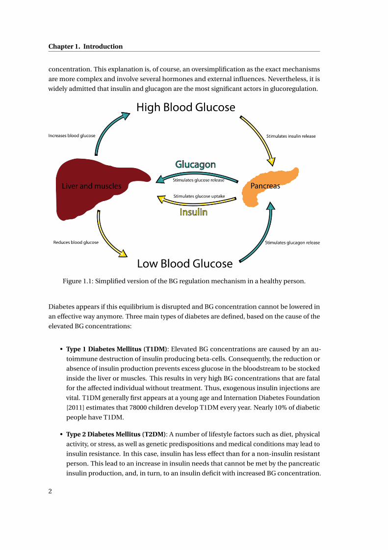
List of Figures1.1 Simplified version of the BG regulation mechanism in a healthy person. . . . . 2
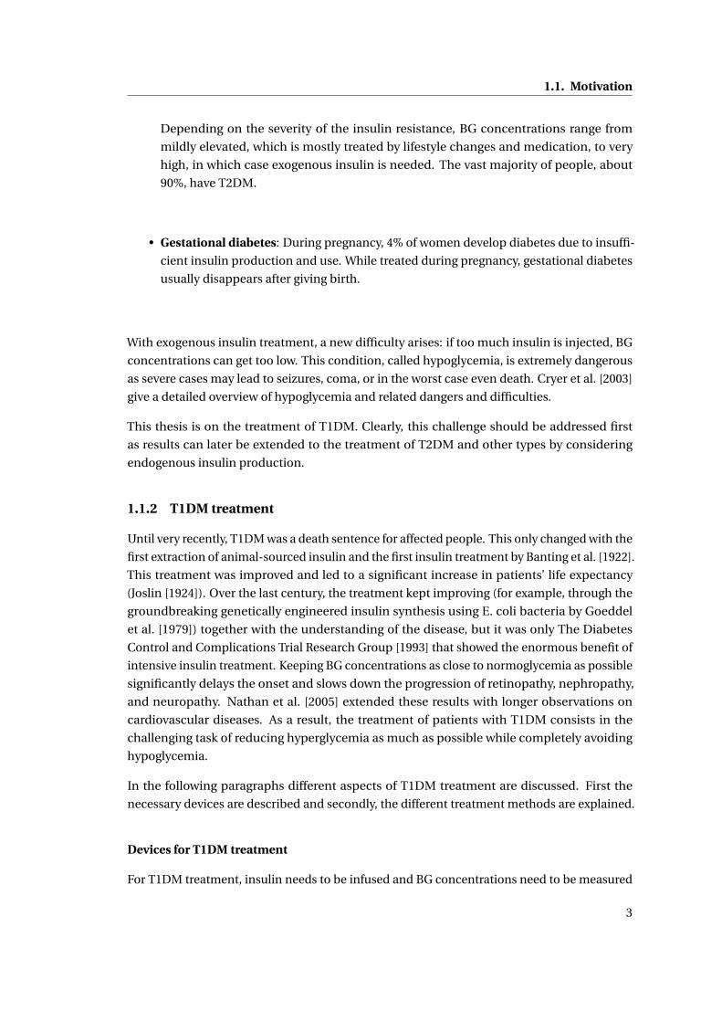
1.2 Illustration of standard therapy. . . . . . . . . . . . . . . . . . . . . . . . . . . . . 5
1.3 Illustration of a system. . . . . . . . . . . . . . . . . . . . . . . . . . . . . . . . . . 6
1.4 Illustration of open-loop control for T1DM treatment. . . . . . . . . . . . . . . . 7
1.5 Illustration of closed-loop control for T1DM treatment. . . . . . . . . . . . . . . 7
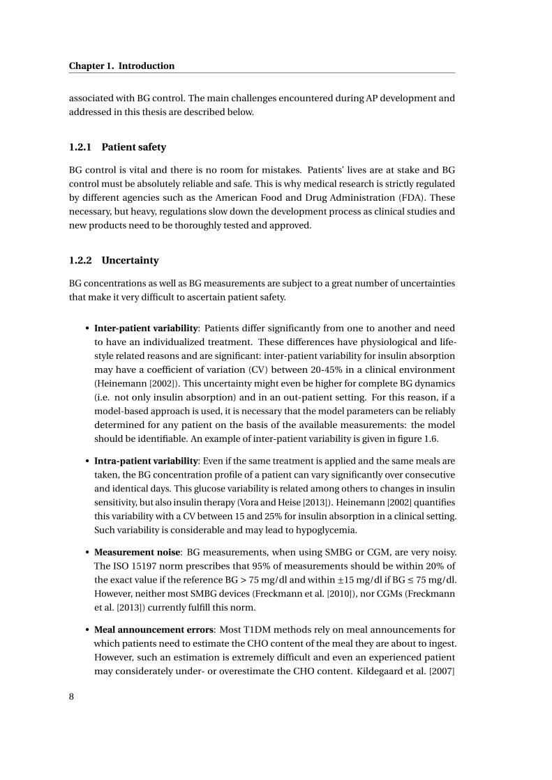
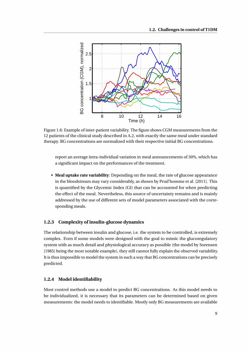
1.6 Example of inter-patient variability. The figure shows CGM measurements from
the 12 patients of the clinical study described in A.2, with exactly the same meal
under standard therapy. BG concentrations are normalized with their respective
initial BG concentrations. . . . . . . . . . . . . . . . . . . . . . . . . . . . . . . . . 9
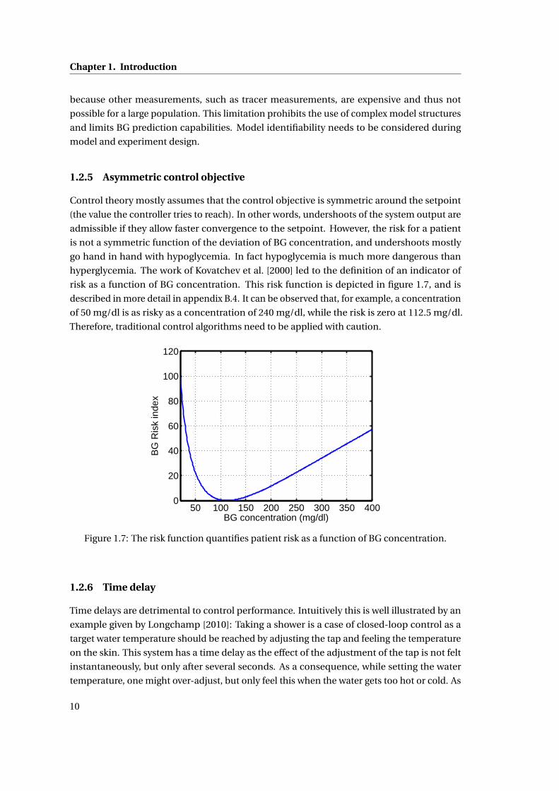
1.7 The risk function quantifies patient risk as a function of BG concentration. . . . 10
2.1 BG predictions using the LMM with the same insulin sensitivity Kx and inputs,
but two different time constants 1/ax . . . . . . . . . . . . . . . . . . . . . . . . . . 25
2.2 BG predictions using the TPM with the same insulin sensitivity Kx and inputs,
but two different time constants 1/ax . . . . . . . . . . . . . . . . . . . . . . . . . . 26
2.3 TPM simulations after an insulin bolus (left-hand side) and a meal (right-hand
side) . . . . . . . . . . . . . . . . . . . . . . . . . . . . . . . . . . . . . . . . . . . . . 29
2.4 Simulations of the TPM with simultaneous insulin bolus and meal (left) and
only an insulin bolus (right). The parameters are chosen as follows: ax = 0.04,
ag = 0.03,Kg
Kx(= I 2C ) = 0.1 and Kx is chosen according to legend. The insulin
bolus is 2U and the meal is 20g . . . . . . . . . . . . . . . . . . . . . . . . . . . . . 32
2.5 Boxplot (cf. appendix B.9) of the MAD and R2 of the data fit of every patient
(n=10). Comparison between different prediction models on UVa simulator data. 33
2.6 Comparison of physician-set therapy parameters and identified model parame-
ters to illustrate correlation results on UVa simulator data (n=10). . . . . . . . . 35
2.7 MAD (top) and % in EGA zone A (bottom) of the averaged model predictions
(n=40) for the different prediction models and prediction horizons h on UVa
simulator data. Mean values are given on the left, standard deviations on the right. 37
2.8 Example of data fits for different prediction models on clinical data. . . . . . . . 38
2.9 Boxplot (cf. appendix B.9) of the MAD and R2 of the data fit of every patient
(n=10). Comparison between different prediction models on clinical data. . . . 39
2.10 Comparison of physician-set therapy parameters and identified model parame-
ters to illustrate correlation results on clinical data. . . . . . . . . . . . . . . . . . 41
xvii
List of Figures
2.11 Example of 90 minute predictions for different prediction models on clinical data. 42
2.12 MAD (top) and % in EGA zone A (bottom) of the averaged model predictions
(n=58) for the different prediction models on clinical data. Mean values are given
on the left, standard deviations on the right. . . . . . . . . . . . . . . . . . . . . . 43
3.1 Scenario 1: Example of 5 realizations of the sTPM (left) and estimation of 95%
confidence interval (right). . . . . . . . . . . . . . . . . . . . . . . . . . . . . . . . 55
3.2 Scenario 2: Example of 5 realizations of the sTPM (left) and estimation of 95%
confidence interval (right). . . . . . . . . . . . . . . . . . . . . . . . . . . . . . . . 55
3.3 Boxplot (cf. appendix B.9) of percentage of measurements inside the 95% confi-
dence interval of all validation data sets (n=40) for cases 1-4. . . . . . . . . . . . 58
3.4 Examples for cases 1 to 4. . . . . . . . . . . . . . . . . . . . . . . . . . . . . . . . . 59
3.5 Examples for case 2 when validating over the complete data set. . . . . . . . . . 60
3.6 Examples for case 4 when validating over the complete data set. Both examples
show the negative influence of their identical noise realization. . . . . . . . . . . 60
3.7 Boxplot (cf. appendix B.9) of expected percentage of measurements inside the
95% confidence interval of all validation data sets for cases 5 to 8. . . . . . . . . 61
3.8 Comparison of stochastic prediction for cases 5 and 6. . . . . . . . . . . . . . . . 62
3.9 Examples for different cases on 90 minutes prediction horizon. . . . . . . . . . . 63
3.10 Prediction results for UVa simulator results (cases 1-4) for different horizons.
Means and standard deviations evaluated on all 40 validation sets are given.
Mean values are given on the left, standard deviations on the right. . . . . . . . 64
3.11 Prediction results for clinical study results (cases 5-8) for different horizons.
Means and standard deviations evaluated on all validation sets are given. Mean
values are given on the left, standard deviations on the right. . . . . . . . . . . . 65
3.12 Stochastic prediction results for different models for case 2 and case 6. Mean
values are given on the left, standard deviations on the right. . . . . . . . . . . . 65
4.1 Luenberger observer . . . . . . . . . . . . . . . . . . . . . . . . . . . . . . . . . . . 72
4.2 Boxplot (cf. appendix B.9) of average percentage in zone A of the EGA and
Boxplot of average MAD for scenario 1, corresponding to day 3 of the validation
data set. . . . . . . . . . . . . . . . . . . . . . . . . . . . . . . . . . . . . . . . . . . . 78
4.3 Example of a BG profile on scenario 1 for adult 5. . . . . . . . . . . . . . . . . . . 78
4.4 Boxplot (cf. appendix B.9) of average percentage in zone A of the EGA and
Boxplot of average MAD for scenario 2, corresponding to day 4 of the validation
data set. . . . . . . . . . . . . . . . . . . . . . . . . . . . . . . . . . . . . . . . . . . . 79
4.5 Example of a BG profile on scenario 2 for adult 6. . . . . . . . . . . . . . . . . . . 79
4.6 Boxplot (cf. appendix B.9) of average percentage in zone A of the EGA and
Boxplot of average MAD for scenario 2, corresponding to day 4 of the validation
data set. . . . . . . . . . . . . . . . . . . . . . . . . . . . . . . . . . . . . . . . . . . . 80
4.7 Example of a BG profile on scenario 2 for adult 6. . . . . . . . . . . . . . . . . . . 81
5.1 Insulin-glucose system with meal disturbance. . . . . . . . . . . . . . . . . . . . 86
xviii
List of Figures
5.2 Insulin-glucose system with meal disturbance and feed-forward control. . . . . 87
5.3 Proportional controller. . . . . . . . . . . . . . . . . . . . . . . . . . . . . . . . . . 104
5.4 The TPC. . . . . . . . . . . . . . . . . . . . . . . . . . . . . . . . . . . . . . . . . . . 107
5.5 Closed-loop controller with announced meal and filter. . . . . . . . . . . . . . . 109
5.6 Closed-loop controller without meal announcement. . . . . . . . . . . . . . . . 110
5.7 Averages of different metrics as a function of τ. . . . . . . . . . . . . . . . . . . . 110
5.8 Results for Adult 9 on nominal scenario with TPC TPF. . . . . . . . . . . . . . . . 111
5.9 Results for Adult 1 on nominal scenario with TPC TPF. . . . . . . . . . . . . . . . 112
5.10 Example of a BG concentration profile for adult 5 on the nominal scenario with
the TPC NM (unannounced meals). . . . . . . . . . . . . . . . . . . . . . . . . . . 115
5.11 Relative BGRI error as a function of the number of repetitions for Adult 1 and a
PID controller. . . . . . . . . . . . . . . . . . . . . . . . . . . . . . . . . . . . . . . . 125
A.1 Example of UVa simulation of Adult 6 on nominal day scenario. . . . . . . . . . 133
B.1 Clarke EGA. Figure based on MATLAB code by Edgar Guevara Codina. . . . . . 138
C.1 Blood glucose concentration and heart rate for patient 9 on day 2. Illustration of
linear regression (red line). 1 mmol/l corresponds to 18 mg/dl. . . . . . . . . . . 144
C.2 Comparison of slopes for different patients. Values for both exercise sessions
and their mean are shown. 1 mmol/l corresponds to 18 mg/dl. . . . . . . . . . . 145
C.3 Model fit for patient 9 for both days. 1 mmol/l corresponds to 18 mg/dl. . . . . 147
xix

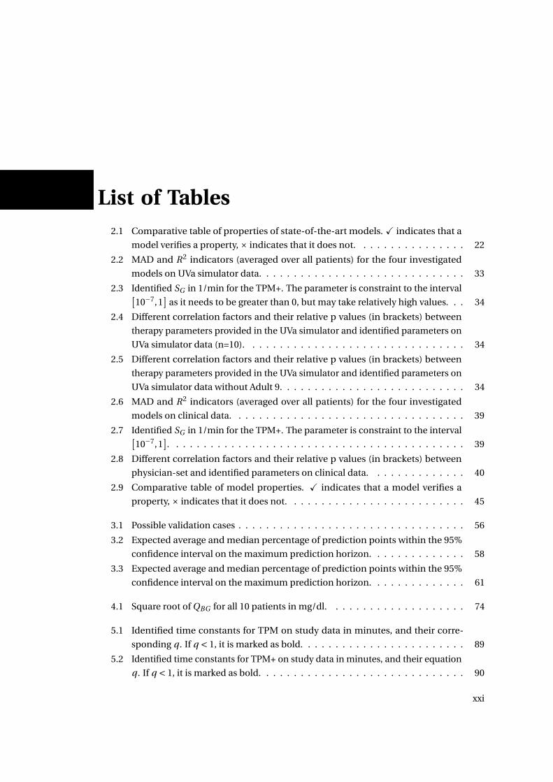
List of Tables2.1 Comparative table of properties of state-of-the-art models. X indicates that a
model verifies a property, × indicates that it does not. . . . . . . . . . . . . . . . 22
2.2 MAD and R2 indicators (averaged over all patients) for the four investigated
models on UVa simulator data. . . . . . . . . . . . . . . . . . . . . . . . . . . . . . 33
2.3 Identified SG in 1/min for the TPM+. The parameter is constraint to the interval[10−7,1
]as it needs to be greater than 0, but may take relatively high values. . . 34
2.4 Different correlation factors and their relative p values (in brackets) between
therapy parameters provided in the UVa simulator and identified parameters on
UVa simulator data (n=10). . . . . . . . . . . . . . . . . . . . . . . . . . . . . . . . 34
2.5 Different correlation factors and their relative p values (in brackets) between
therapy parameters provided in the UVa simulator and identified parameters on
UVa simulator data without Adult 9. . . . . . . . . . . . . . . . . . . . . . . . . . . 34
2.6 MAD and R2 indicators (averaged over all patients) for the four investigated
models on clinical data. . . . . . . . . . . . . . . . . . . . . . . . . . . . . . . . . . 39
2.7 Identified SG in 1/min for the TPM+. The parameter is constraint to the interval[10−7,1
]. . . . . . . . . . . . . . . . . . . . . . . . . . . . . . . . . . . . . . . . . . . 39
2.8 Different correlation factors and their relative p values (in brackets) between
physician-set and identified parameters on clinical data. . . . . . . . . . . . . . 40
2.9 Comparative table of model properties. X indicates that a model verifies a
property, × indicates that it does not. . . . . . . . . . . . . . . . . . . . . . . . . . 45
3.1 Possible validation cases . . . . . . . . . . . . . . . . . . . . . . . . . . . . . . . . . 56
3.2 Expected average and median percentage of prediction points within the 95%
confidence interval on the maximum prediction horizon. . . . . . . . . . . . . . 58
3.3 Expected average and median percentage of prediction points within the 95%
confidence interval on the maximum prediction horizon. . . . . . . . . . . . . . 61
4.1 Square root of QBG for all 10 patients in mg/dl. . . . . . . . . . . . . . . . . . . . 74
5.1 Identified time constants for TPM on study data in minutes, and their corre-
sponding q . If q < 1, it is marked as bold. . . . . . . . . . . . . . . . . . . . . . . . 89
5.2 Identified time constants for TPM+ on study data in minutes, and their equation
q . If q < 1, it is marked as bold. . . . . . . . . . . . . . . . . . . . . . . . . . . . . . 90
xxi
List of Tables
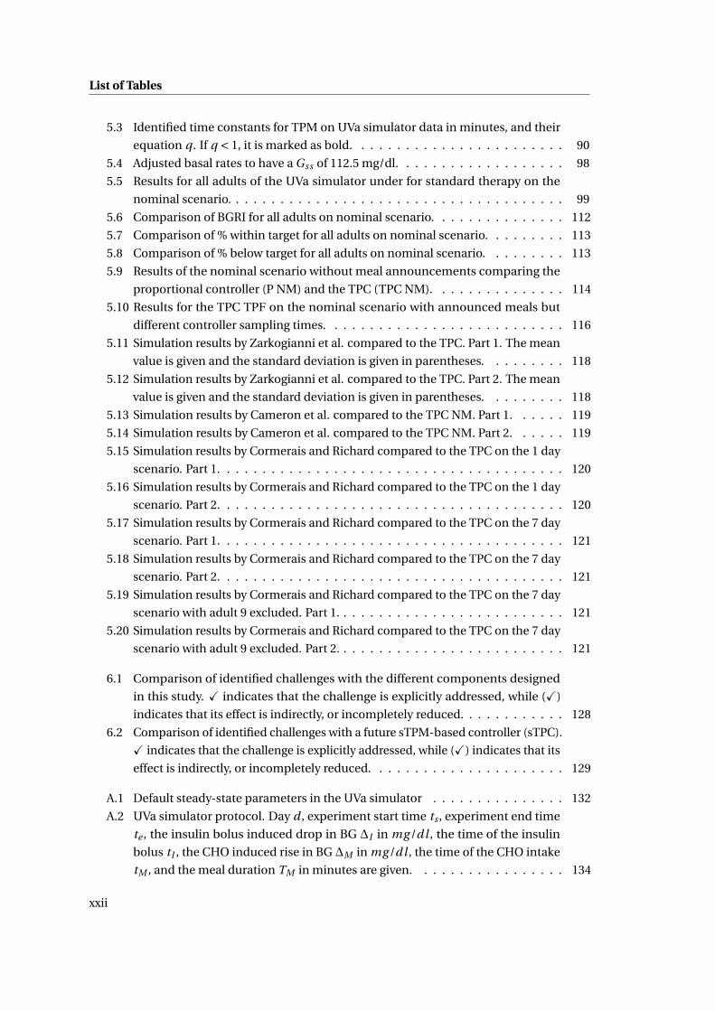
5.3 Identified time constants for TPM on UVa simulator data in minutes, and their
equation q . If q < 1, it is marked as bold. . . . . . . . . . . . . . . . . . . . . . . . 90
5.4 Adjusted basal rates to have a Gss of 112.5 mg/dl. . . . . . . . . . . . . . . . . . . 98
5.5 Results for all adults of the UVa simulator under for standard therapy on the
nominal scenario. . . . . . . . . . . . . . . . . . . . . . . . . . . . . . . . . . . . . . 99
5.6 Comparison of BGRI for all adults on nominal scenario. . . . . . . . . . . . . . . 112
5.7 Comparison of % within target for all adults on nominal scenario. . . . . . . . . 113
5.8 Comparison of % below target for all adults on nominal scenario. . . . . . . . . 113
5.9 Results of the nominal scenario without meal announcements comparing the
proportional controller (P NM) and the TPC (TPC NM). . . . . . . . . . . . . . . 114
5.10 Results for the TPC TPF on the nominal scenario with announced meals but
different controller sampling times. . . . . . . . . . . . . . . . . . . . . . . . . . . 116
5.11 Simulation results by Zarkogianni et al. compared to the TPC. Part 1. The mean
value is given and the standard deviation is given in parentheses. . . . . . . . . 118
5.12 Simulation results by Zarkogianni et al. compared to the TPC. Part 2. The mean
value is given and the standard deviation is given in parentheses. . . . . . . . . 118
5.13 Simulation results by Cameron et al. compared to the TPC NM. Part 1. . . . . . 119
5.14 Simulation results by Cameron et al. compared to the TPC NM. Part 2. . . . . . 119
5.15 Simulation results by Cormerais and Richard compared to the TPC on the 1 day
scenario. Part 1. . . . . . . . . . . . . . . . . . . . . . . . . . . . . . . . . . . . . . . 120
5.16 Simulation results by Cormerais and Richard compared to the TPC on the 1 day
scenario. Part 2. . . . . . . . . . . . . . . . . . . . . . . . . . . . . . . . . . . . . . . 120
5.17 Simulation results by Cormerais and Richard compared to the TPC on the 7 day
scenario. Part 1. . . . . . . . . . . . . . . . . . . . . . . . . . . . . . . . . . . . . . . 121
5.18 Simulation results by Cormerais and Richard compared to the TPC on the 7 day
scenario. Part 2. . . . . . . . . . . . . . . . . . . . . . . . . . . . . . . . . . . . . . . 121
5.19 Simulation results by Cormerais and Richard compared to the TPC on the 7 day
scenario with adult 9 excluded. Part 1. . . . . . . . . . . . . . . . . . . . . . . . . . 121
5.20 Simulation results by Cormerais and Richard compared to the TPC on the 7 day
scenario with adult 9 excluded. Part 2. . . . . . . . . . . . . . . . . . . . . . . . . . 121
6.1 Comparison of identified challenges with the different components designed
in this study. X indicates that the challenge is explicitly addressed, while (X)
indicates that its effect is indirectly, or incompletely reduced. . . . . . . . . . . . 128
6.2 Comparison of identified challenges with a future sTPM-based controller (sTPC).
X indicates that the challenge is explicitly addressed, while (X) indicates that its
effect is indirectly, or incompletely reduced. . . . . . . . . . . . . . . . . . . . . . 129
A.1 Default steady-state parameters in the UVa simulator . . . . . . . . . . . . . . . 132
A.2 UVa simulator protocol. Day d , experiment start time ts , experiment end time
te , the insulin bolus induced drop in BG ∆I in mg /dl , the time of the insulin
bolus tI , the CHO induced rise in BG ∆M in mg /dl , the time of the CHO intake
tM , and the meal duration TM in minutes are given. . . . . . . . . . . . . . . . . 134
xxii
List of Tables
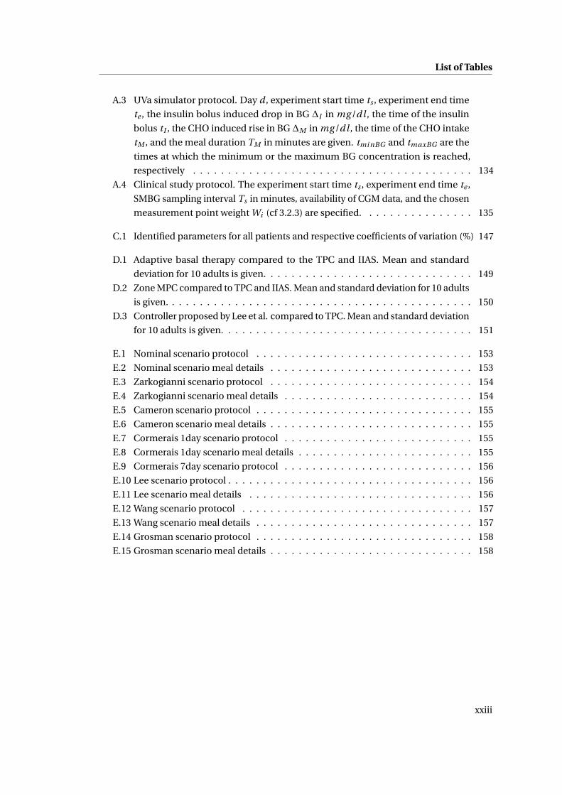
A.3 UVa simulator protocol. Day d , experiment start time ts , experiment end time
te , the insulin bolus induced drop in BG ∆I in mg /dl , the time of the insulin
bolus tI , the CHO induced rise in BG ∆M in mg /dl , the time of the CHO intake
tM , and the meal duration TM in minutes are given. tmi nBG and tmaxBG are the
times at which the minimum or the maximum BG concentration is reached,
respectively . . . . . . . . . . . . . . . . . . . . . . . . . . . . . . . . . . . . . . . . 134
A.4 Clinical study protocol. The experiment start time ts , experiment end time te ,
SMBG sampling interval Ts in minutes, availability of CGM data, and the chosen
measurement point weight Wi (cf 3.2.3) are specified. . . . . . . . . . . . . . . . 135
C.1 Identified parameters for all patients and respective coefficients of variation (%) 147
D.1 Adaptive basal therapy compared to the TPC and IIAS. Mean and standard
deviation for 10 adults is given. . . . . . . . . . . . . . . . . . . . . . . . . . . . . . 149
D.2 Zone MPC compared to TPC and IIAS. Mean and standard deviation for 10 adults
is given. . . . . . . . . . . . . . . . . . . . . . . . . . . . . . . . . . . . . . . . . . . . 150
D.3 Controller proposed by Lee et al. compared to TPC. Mean and standard deviation
for 10 adults is given. . . . . . . . . . . . . . . . . . . . . . . . . . . . . . . . . . . . 151
E.1 Nominal scenario protocol . . . . . . . . . . . . . . . . . . . . . . . . . . . . . . . 153
E.2 Nominal scenario meal details . . . . . . . . . . . . . . . . . . . . . . . . . . . . . 153
E.3 Zarkogianni scenario protocol . . . . . . . . . . . . . . . . . . . . . . . . . . . . . 154
E.4 Zarkogianni scenario meal details . . . . . . . . . . . . . . . . . . . . . . . . . . . 154
E.5 Cameron scenario protocol . . . . . . . . . . . . . . . . . . . . . . . . . . . . . . . 155
E.6 Cameron scenario meal details . . . . . . . . . . . . . . . . . . . . . . . . . . . . . 155
E.7 Cormerais 1day scenario protocol . . . . . . . . . . . . . . . . . . . . . . . . . . . 155
E.8 Cormerais 1day scenario meal details . . . . . . . . . . . . . . . . . . . . . . . . . 155
E.9 Cormerais 7day scenario protocol . . . . . . . . . . . . . . . . . . . . . . . . . . . 156
E.10 Lee scenario protocol . . . . . . . . . . . . . . . . . . . . . . . . . . . . . . . . . . . 156
E.11 Lee scenario meal details . . . . . . . . . . . . . . . . . . . . . . . . . . . . . . . . 156
E.12 Wang scenario protocol . . . . . . . . . . . . . . . . . . . . . . . . . . . . . . . . . 157
E.13 Wang scenario meal details . . . . . . . . . . . . . . . . . . . . . . . . . . . . . . . 157
E.14 Grosman scenario protocol . . . . . . . . . . . . . . . . . . . . . . . . . . . . . . . 158
E.15 Grosman scenario meal details . . . . . . . . . . . . . . . . . . . . . . . . . . . . . 158
xxiii

1 Introduction
1.1 Motivation
1.1.1 Diabetes Mellitus
Diabetes Mellitus is a metabolic disease characterized by elevated Blood Glucose (BG) concen-
trations causing acute symptoms such as polyuria (frequent urination), polydipsia (increased
thirst), and polyphagia (increased hunger). If these high BG concentrations stay untreated
- a condition called hyperglycemia - severe short-term complications including diabetic ke-
toacidosis and coma may occur. However, long-term complications due to prolonged hy-
perglycemia are currently the most expensive burden to health care systems and the biggest
detriment patient well-being. These complications include cardiovascular diseases, chronic
renal failure, and nerve damages, leading among others to blindness, ulceration, amputations,
and the need for dialysis.
In 2012, more than 371 million people (Internation Diabetes Foundation [2011]), i.e. 8.3%
of the adult world population, are deemed to suffer from diabetes, most of which in low-
and middle- income countries. This enormous, and constantly increasing (Danaei et al.
[2011]) prevalence generates global health care expenditures estimated at 465 billion USD
in 2011 (expected to rise to 595 billion USD by 2030). These figures highlight the primordial
importance of research in diabetes prevention and care.
For a healthy person, the regulation of BG concentrations can be described by the simplified
mechanism illustrated in figure 1.1. BG concentrations are kept in balance around 100 mg/dl
mainly because of the effects of two hormones: insulin and glucagon. These hormones are
produced by the beta- and alpha-cells of the pancreas, respectively. If BG concentration
increases, for instance because of a meal, insulin release is stimulated. This insulin mediates
the uptake of glucose from the blood to be stocked in the liver and muscles in the form
of glycogen, thus reducing BG concentrations to a normal level. If, on the other hand, BG
concentrations are low, glucagon is released by the pancreas. Glucagon stimulates the release
of the stocked glycogen from the liver and muscles to the bloodstream, thus increasing BG
1
Chapter 1. Introduction
concentration. This explanation is, of course, an oversimplification as the exact mechanisms
are more complex and involve several hormones and external influences. Nevertheless, it is
widely admitted that insulin and glucagon are the most significant actors in glucoregulation.
Figure 1.1: Simplified version of the BG regulation mechanism in a healthy person.
Diabetes appears if this equilibrium is disrupted and BG concentration cannot be lowered in
an effective way anymore. Three main types of diabetes are defined, based on the cause of the
elevated BG concentrations:
• Type 1 Diabetes Mellitus (T1DM): Elevated BG concentrations are caused by an au-
toimmune destruction of insulin producing beta-cells. Consequently, the reduction or
absence of insulin production prevents excess glucose in the bloodstream to be stocked
inside the liver or muscles. This results in very high BG concentrations that are fatal
for the affected individual without treatment. Thus, exogenous insulin injections are
vital. T1DM generally first appears at a young age and Internation Diabetes Foundation
[2011] estimates that 78000 children develop T1DM every year. Nearly 10% of diabetic
people have T1DM.
• Type 2 Diabetes Mellitus (T2DM): A number of lifestyle factors such as diet, physical
activity, or stress, as well as genetic predispositions and medical conditions may lead to
insulin resistance. In this case, insulin has less effect than for a non-insulin resistant
person. This lead to an increase in insulin needs that cannot be met by the pancreatic
insulin production, and, in turn, to an insulin deficit with increased BG concentration.
2
1.1. Motivation
Depending on the severity of the insulin resistance, BG concentrations range from
mildly elevated, which is mostly treated by lifestyle changes and medication, to very
high, in which case exogenous insulin is needed. The vast majority of people, about
90%, have T2DM.
• Gestational diabetes: During pregnancy, 4% of women develop diabetes due to insuffi-
cient insulin production and use. While treated during pregnancy, gestational diabetes
usually disappears after giving birth.
With exogenous insulin treatment, a new difficulty arises: if too much insulin is injected, BG
concentrations can get too low. This condition, called hypoglycemia, is extremely dangerous
as severe cases may lead to seizures, coma, or in the worst case even death. Cryer et al. [2003]
give a detailed overview of hypoglycemia and related dangers and difficulties.
This thesis is on the treatment of T1DM. Clearly, this challenge should be addressed first
as results can later be extended to the treatment of T2DM and other types by considering
endogenous insulin production.
1.1.2 T1DM treatment
Until very recently, T1DM was a death sentence for affected people. This only changed with the
first extraction of animal-sourced insulin and the first insulin treatment by Banting et al. [1922].
This treatment was improved and led to a significant increase in patients’ life expectancy
(Joslin [1924]). Over the last century, the treatment kept improving (for example, through the
groundbreaking genetically engineered insulin synthesis using E. coli bacteria by Goeddel
et al. [1979]) together with the understanding of the disease, but it was only The Diabetes
Control and Complications Trial Research Group [1993] that showed the enormous benefit of
intensive insulin treatment. Keeping BG concentrations as close to normoglycemia as possible
significantly delays the onset and slows down the progression of retinopathy, nephropathy,
and neuropathy. Nathan et al. [2005] extended these results with longer observations on
cardiovascular diseases. As a result, the treatment of patients with T1DM consists in the
challenging task of reducing hyperglycemia as much as possible while completely avoiding
hypoglycemia.
In the following paragraphs different aspects of T1DM treatment are discussed. First the
necessary devices are described and secondly, the different treatment methods are explained.
Devices for T1DM treatment
For T1DM treatment, insulin needs to be infused and BG concentrations need to be measured
3
Chapter 1. Introduction
Insulin administration Insulin can be administered by several means. Although syringes
have been used for a long time for injecting insulin boluses (single doses), they are now widely
replaced by insulin pens. For the last decades, the use of insulin pumps has become more and
more widespread. These devices allow almost continuous insulin infusion by giving boluses
up to every minute. Insulin may be administered (i) subcutaneously (SC), i.e. beneath the skin,
(ii) intraperitoneally (IP),i.e. into the membrane of the abdominal cavity, or (iii) intravenously
(IV), i.e. directly into the veins. The SC route is the standard for commercial insulin pumps
because of the low risk of infections, but has the drawback of relatively slow insulin uptake
times. Since fast insulin action reduces the amplitude postprandial BG excursions (as will
be shown later), faster IP delivery is being researched and shows promising results, but with
the risk of complications (Liebl et al. [2009]). IV infusion is the fastest as it is the closest to
healthy insulin delivery, but is only applicable within a clinical setting because of a high risk of
infection. In this thesis, therapy using Continuous Subcutaneous Insulin Infusion (CSII) is
investigated because of the possibility to infuse insulin almost continuously and because of
its widespread acceptance and use.
BG measurements Accurate BG measurements are key for appropriate treatment and avoid-
ance of hypoglycemia. Two main methods are commonly being used: Self Monitoring of Blood
Glucose (SMBG) and Continuous Glucose Monitoring (CGM). SMBG consists in measuring the
glucose concentration in a small drop of blood obtained by pricking the finger with a lancet.
This method is by far the most common because of its relatively good accuracy at reasonable
cost. The biggest drawback of this method is that for every measurement, the patient needs
to extract a blood drop - a painful procedure. As as results most patients do not take BG
measurements very frequently. CGM devices are an alternative that gives almost continuous
BG concentrations with less finger pricks, at the price of reduced accuracy and reliability.
Also, these devices are relatively expensive and have a time-lag that can be dangerous. These
disadvantages explain its slow progression on the market. This work considers both types of
measurements.
Diabetes treatment methods
Different T1DM treatment approaches, ranging from currently applied methods to active
research fields, are introduced in this paragraph.
Standard therapy Currently, standard therapy - as it will be called in this thesis - is the norm
when it comes to T1DM treatment. This therapy is also referred to as basal/bolus therapy or
Multiple Daily Injections (MDI), if performed using insulin pens or syringes. The principle is
to split insulin treatment into two parts as illustrated in figure 1.2.
• basal insulin is insulin that acts relatively uniformly throughout the day and should
keep patients fasting BG concentration close to the optimum. Patients using syringes or
4
1.1. Motivation
pens inject long-acting insulin once or twice a day while CSII-treated patients use the
insulin pump to adjust the basal rate in an "optimal" manner. Currently, the ability to
change the basal insulin whenever needed is a major advantage of CSII over syringes or
pens. A good overview of CSII treatment is given by Marcus [2013].
• bolus insulin is insulin that is injected in order to counteract the effect of meals. The
carbohydrates (CHO) contained in meals are processed by the digestive system and
release glucose into the bloodstream. In order to avoid hyperglycemia, this major
disturbance needs to be counteracted by injecting a well-chosen quantity of fast-acting
insulin using a syringe, pen, or insulin pump. This quantity is based on the quantity
of ingested CHO and the pre-meal BG concentration. To compute the correct insulin
amount, the patient has to take an SMBG measurement before each meal.
The Diabetes Control and Complications Trial Research Group [1993] that standard therapy
is effective. However, this method can be enhanced by taking into account the additional
information provided by CGM devices on the one hand, and by making meal rejections more
effective on the other hand. Indeed, according to Prud’homme et al. [2011] these have a lot
of room for improvement, as different meal speeds are not taken into account in standard
therapy.
Figure 1.2: Illustration of standard therapy.
Short introduction to systems and control Before describing more elaborate control meth-
ods, control-specific concepts and vocabulary are introduced. In the context of control, a
system, represented in figure 1.3, is an object of interest (it can be many different things) upon
which different actions can be taken - the inputs u - and that shows or gives different reactions
- the outputs y . The inputs are defined by the fact that they can be manipulated from outside
the system, while the outputs are defined by the property that they can be observed from
outside the system. Additionally, disturbances may apply to the systems. These are generally
5
Chapter 1. Introduction
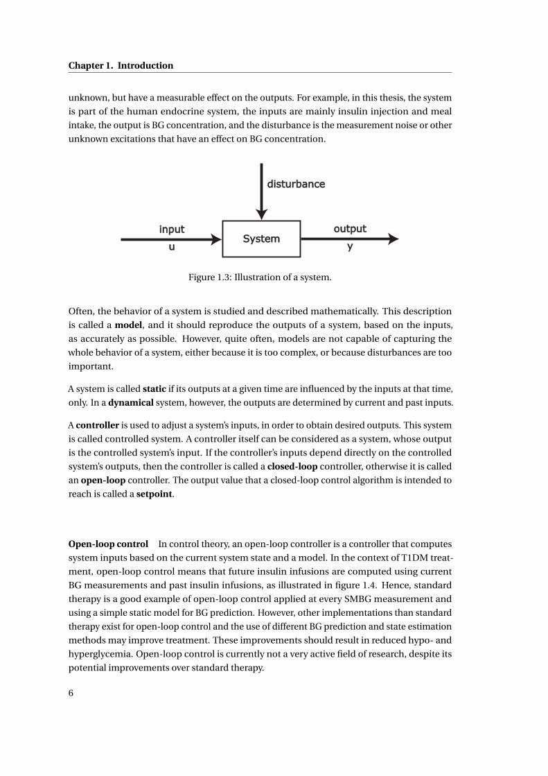
unknown, but have a measurable effect on the outputs. For example, in this thesis, the system
is part of the human endocrine system, the inputs are mainly insulin injection and meal
intake, the output is BG concentration, and the disturbance is the measurement noise or other
unknown excitations that have an effect on BG concentration.
Figure 1.3: Illustration of a system.
Often, the behavior of a system is studied and described mathematically. This description
is called a model, and it should reproduce the outputs of a system, based on the inputs,
as accurately as possible. However, quite often, models are not capable of capturing the
whole behavior of a system, either because it is too complex, or because disturbances are too
important.
A system is called static if its outputs at a given time are influenced by the inputs at that time,
only. In a dynamical system, however, the outputs are determined by current and past inputs.
A controller is used to adjust a system’s inputs, in order to obtain desired outputs. This system
is called controlled system. A controller itself can be considered as a system, whose output
is the controlled system’s input. If the controller’s inputs depend directly on the controlled
system’s outputs, then the controller is called a closed-loop controller, otherwise it is called
an open-loop controller. The output value that a closed-loop control algorithm is intended to
reach is called a setpoint.
Open-loop control In control theory, an open-loop controller is a controller that computes
system inputs based on the current system state and a model. In the context of T1DM treat-
ment, open-loop control means that future insulin infusions are computed using current
BG measurements and past insulin infusions, as illustrated in figure 1.4. Hence, standard
therapy is a good example of open-loop control applied at every SMBG measurement and
using a simple static model for BG prediction. However, other implementations than standard
therapy exist for open-loop control and the use of different BG prediction and state estimation
methods may improve treatment. These improvements should result in reduced hypo- and
hyperglycemia. Open-loop control is currently not a very active field of research, despite its
potential improvements over standard therapy.
6
1.2. Challenges in control of T1DM
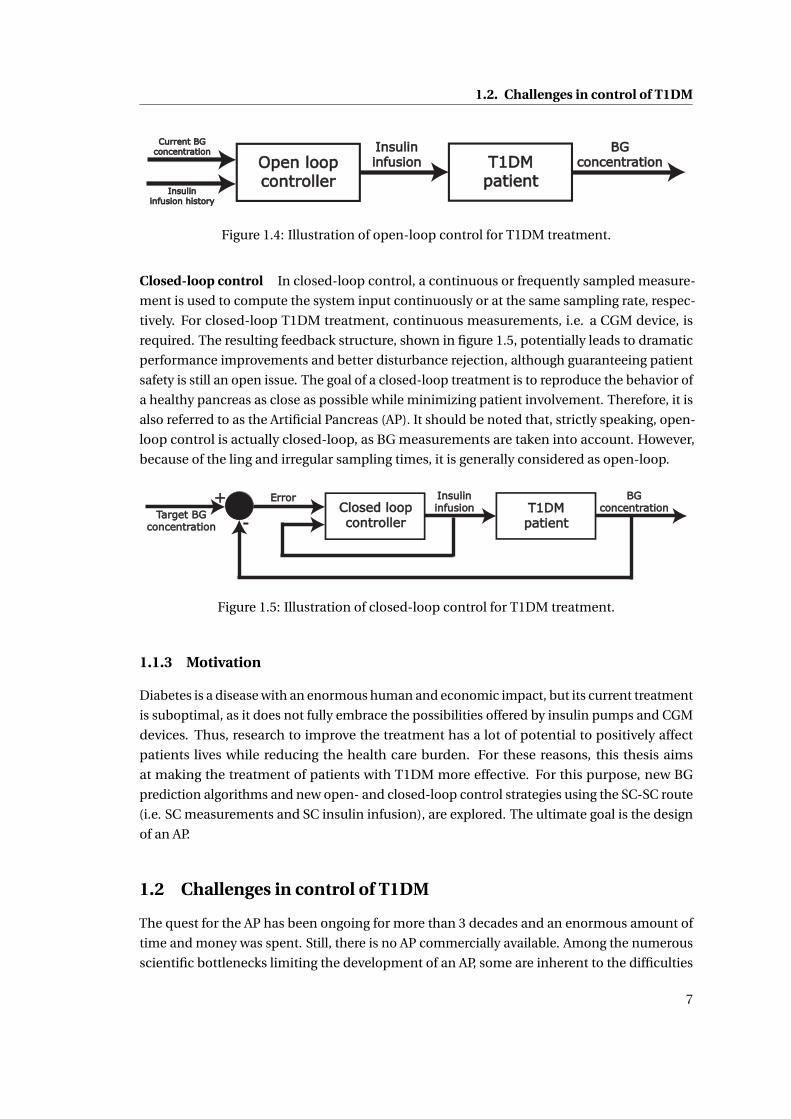
Figure 1.4: Illustration of open-loop control for T1DM treatment.
Closed-loop control In closed-loop control, a continuous or frequently sampled measure-
ment is used to compute the system input continuously or at the same sampling rate, respec-
tively. For closed-loop T1DM treatment, continuous measurements, i.e. a CGM device, is
required. The resulting feedback structure, shown in figure 1.5, potentially leads to dramatic
performance improvements and better disturbance rejection, although guaranteeing patient
safety is still an open issue. The goal of a closed-loop treatment is to reproduce the behavior of
a healthy pancreas as close as possible while minimizing patient involvement. Therefore, it is
also referred to as the Artificial Pancreas (AP). It should be noted that, strictly speaking, open-
loop control is actually closed-loop, as BG measurements are taken into account. However,
because of the ling and irregular sampling times, it is generally considered as open-loop.
Figure 1.5: Illustration of closed-loop control for T1DM treatment.
1.1.3 Motivation
Diabetes is a disease with an enormous human and economic impact, but its current treatment
is suboptimal, as it does not fully embrace the possibilities offered by insulin pumps and CGM
devices. Thus, research to improve the treatment has a lot of potential to positively affect
patients lives while reducing the health care burden. For these reasons, this thesis aims
at making the treatment of patients with T1DM more effective. For this purpose, new BG
prediction algorithms and new open- and closed-loop control strategies using the SC-SC route
(i.e. SC measurements and SC insulin infusion), are explored. The ultimate goal is the design
of an AP.
1.2 Challenges in control of T1DM
The quest for the AP has been ongoing for more than 3 decades and an enormous amount of
time and money was spent. Still, there is no AP commercially available. Among the numerous
scientific bottlenecks limiting the development of an AP, some are inherent to the difficulties
7
Chapter 1. Introduction
associated with BG control. The main challenges encountered during AP development and
addressed in this thesis are described below.
1.2.1 Patient safety
BG control is vital and there is no room for mistakes. Patients’ lives are at stake and BG
control must be absolutely reliable and safe. This is why medical research is strictly regulated
by different agencies such as the American Food and Drug Administration (FDA). These
necessary, but heavy, regulations slow down the development process as clinical studies and
new products need to be thoroughly tested and approved.
1.2.2 Uncertainty
BG concentrations as well as BG measurements are subject to a great number of uncertainties
that make it very difficult to ascertain patient safety.
• Inter-patient variability: Patients differ significantly from one to another and need
to have an individualized treatment. These differences have physiological and life-
style related reasons and are significant: inter-patient variability for insulin absorption
may have a coefficient of variation (CV) between 20-45% in a clinical environment
(Heinemann [2002]). This uncertainty might even be higher for complete BG dynamics
(i.e. not only insulin absorption) and in an out-patient setting. For this reason, if a
model-based approach is used, it is necessary that the model parameters can be reliably
determined for any patient on the basis of the available measurements: the model
should be identifiable. An example of inter-patient variability is given in figure 1.6.
• Intra-patient variability: Even if the same treatment is applied and the same meals are
taken, the BG concentration profile of a patient can vary significantly over consecutive
and identical days. This glucose variability is related among others to changes in insulin
sensitivity, but also insulin therapy (Vora and Heise [2013]). Heinemann [2002] quantifies
this variability with a CV between 15 and 25% for insulin absorption in a clinical setting.
Such variability is considerable and may lead to hypoglycemia.
• Measurement noise: BG measurements, when using SMBG or CGM, are very noisy.
The ISO 15197 norm prescribes that 95% of measurements should be within 20% of
the exact value if the reference BG > 75 mg/dl and within ±15 mg/dl if BG ≤ 75 mg/dl.
However, neither most SMBG devices (Freckmann et al. [2010]), nor CGMs (Freckmann
et al. [2013]) currently fulfill this norm.
• Meal announcement errors: Most T1DM methods rely on meal announcements for
which patients need to estimate the CHO content of the meal they are about to ingest.
However, such an estimation is extremely difficult and even an experienced patient
may considerately under- or overestimate the CHO content. Kildegaard et al. [2007]
8
1.2. Challenges in control of T1DM
8 10 12 14 16
1
1.5
2
2.5
Time (h)
BG
con
cent
ratio
n (C
GM
), n
orm
aliz
ed
Figure 1.6: Example of inter-patient variability. The figure shows CGM measurements from the12 patients of the clinical study described in A.2, with exactly the same meal under standardtherapy. BG concentrations are normalized with their respective initial BG concentrations.
report an average intra-individual variation in meal announcements of 30%, which has
a significant impact on the performances of the treatment.
• Meal uptake rate variability: Depending on the meal, the rate of glucose appearance
in the bloodstream may vary considerably, as shown by Prud’homme et al. [2011]. This
is quantified by the Glycemic Index (GI) that can be accounted for when predicting
the effect of the meal. Nevertheless, this source of uncertainty remains and is mainly
addressed by the use of different sets of model parameters associated with the corre-
sponding meals.
1.2.3 Complexity of insulin-glucose dynamics
The relationship between insulin and glucose, i.e. the system to be controlled, is extremely
complex. Even if some models were designed with the goal to mimic the glucoregulatory
system with as much detail and physiological accuracy as possible (the model by Sorensen
[1985] being the most notable example), they still cannot fully explain the observed variability.
It is thus impossible to model the system in such a way that BG concentrations can be precisely
predicted.
1.2.4 Model identifiability
Most control methods use a model to predict BG concentrations. As this model needs to
be individualized, it is necessary that its parameters can be determined based on given
measurements: the model needs to identifiable. Mostly only BG measurements are available
9
Chapter 1. Introduction
because other measurements, such as tracer measurements, are expensive and thus not
possible for a large population. This limitation prohibits the use of complex model structures
and limits BG prediction capabilities. Model identifiability needs to be considered during
model and experiment design.
1.2.5 Asymmetric control objective
Control theory mostly assumes that the control objective is symmetric around the setpoint
(the value the controller tries to reach). In other words, undershoots of the system output are
admissible if they allow faster convergence to the setpoint. However, the risk for a patient
is not a symmetric function of the deviation of BG concentration, and undershoots mostly
go hand in hand with hypoglycemia. In fact hypoglycemia is much more dangerous than
hyperglycemia. The work of Kovatchev et al. [2000] led to the definition of an indicator of
risk as a function of BG concentration. This risk function is depicted in figure 1.7, and is
described in more detail in appendix B.4. It can be observed that, for example, a concentration
of 50 mg/dl is as risky as a concentration of 240 mg/dl, while the risk is zero at 112.5 mg/dl.
Therefore, traditional control algorithms need to be applied with caution.
50 100 150 200 250 300 350 4000
20
40
60
80
100
120
BG concentration (mg/dl)
BG
Ris
k in
dex
Figure 1.7: The risk function quantifies patient risk as a function of BG concentration.
1.2.6 Time delay
Time delays are detrimental to control performance. Intuitively this is well illustrated by an
example given by Longchamp [2010]: Taking a shower is a case of closed-loop control as a
target water temperature should be reached by adjusting the tap and feeling the temperature
on the skin. This system has a time delay as the effect of the adjustment of the tap is not felt
instantaneously, but only after several seconds. As a consequence, while setting the water
temperature, one might over-adjust, but only feel this when the water gets too hot or cold. As
10
1.3. Contributions
a reaction, one tends to over-adjust in the other direction and come back close to the original
opening of the tap, hence creating an oscillating system fueled by over-adjustments. For T1DM
control such oscillation must be avoided as they may lead to hypoglycemia or even loss of
controller stability.
During T1DM treatment, time delays have two different origins:
• SC infusion During CSII, insulin is injected subcutaneously. Consequently, the insulin
needs to be transported from the SC compartment into the bloodstream and it takes
some time for the injected insulin to have an effect on BG concentrations. This delay is
generally estimated to be around 20 minutes.
• SC measurement When using a CGM device, BG concentration is measured within the
SC tissue, and not in the plasma. The glucose contained in the blood must first get into
the interstitial fluids, which takes some time. Recently, Basu et al. [2013] estimated this
delay to be 5 to 6 minutes for patients at fasting state (i.e. who did not eat or take an
insulin bolus in the recent past)). However these values might be larger when large BG
variations occur.
Overall, delays of up to 30 minutes between the insulin injection and the measurement of its
effect can be observed. This is a substantial duration, especially considering that, for example,
during exercise BG can drop easily by 60 mg/dl during 30 minutes (cf. figure C.1).
1.2.7 Control saturation
In closed-loop control, the control variable can generally take both, positive and negative
values around its operating point. However, insulin injection can only take positive values
as no insulin can be removed from the body. This saturation makes BG control difficult
because, again, BG concentration undershoots need to be avoided at any price. Such an input
saturation is a strong non-linearity that makes the application of standard control methods
inappropriate and dangerous.
In other words, BG concentration can be lowered by an AP, but they cannot be automatically
increased. The most common ways to increase BG concentration are through CHO intake
or a glucagon shot, but these need to be administered manually. El-Khatib et al. [2010] use a
second pump for automated glucagon injection, but this technique is not widely accepted,
yet.
1.3 Contributions
This thesis proposes to improve the treatment of T1DM while addressing most of the afore-
mentioned challenges using a complete method that leads to state-of-the-art BG control
11
Chapter 1. Introduction
without the need of manual parameter tuning, while making physician supervision more
accessible. The contributions of this work are found in the fields of research discussed in
below:
1.3.1 Control-specific prediction models of T1DM patients
New control-oriented prediction models are proposed. These models allow the identification
of parameters that are directly linked to standard therapy parameters using exclusively BG
measurements. Two versions of the Therapy Parameter-based Model (TPM) were designed
to predict the effect of insulin injections and CHO intake on BG concentrations.
• TPM has only 4 parameters to identify and is best used for predicting BG concentrations
of patients within the University of Virginia/Padova simulator (UVa simulator) - the FDA
approved in silico simulator designed to test control algorithms, and described in A.1.
• TPM+ has 5 parameters to identify and is recommended for prediction of real patient’s
BG concentrations.
Additionally, in the context of this work, a model extension for predicting the effect of physical
activity on BG concentrations was proposed and is given in appendix C.
1.3.2 Stochastic Modeling
A method to design a stochastic model based on a given continuous deterministic model (not
forcibly T1DM related) is proposed and validated. This method reliably computes confidence
intervals on system states based on previous measurements.
This method is applied to the TPM to create the stochastic Therapy Parameter-based Model
(sTPM).
1.3.3 BG Estimation
An Extended Kalman Filter (EKF)-based Therapy Parameter-based Filter (TPF) is proposed
to process CGM data. It takes into account past insulin injections and CHO intake information
to generate improved BG estimations. The TPF is derived using the sTPM.
1.3.4 BG Control
Based on the TPM and the TPF, several novel control approaches are proposed using both,
open- and closed-loop control.
• Open-loop: Standard therapy was extended to reject meal disturbances in a more
12
1.4. Thesis Outline
effective way, especially in the case of very slow acting meals i.e. with a low GI.
• Closed-loop: A new Therapy Parameter-based Controller (TPC) continuously rejects
announced and unannounced disturbances based on the TPM.
1.4 Thesis Outline
The thesis is organized as follows:
Chapter 2 discusses the design of deterministic models that leads to the TPM and TPM+.
These new models are identified and their fitting and prediction capabilities are assessed with
real clinical data as well as UVa simulator data.
In chapter 3, the method to build stochastic models based on parametric uncertainty is
introduced and applied to the TPM to obtain the sTPM. Results are then validated using both
clinical and UVa simulator data.
The use of an EKF in combination with the TPM or sTPM to improve the estimation of BG
concentrations given by CGM devices is discussed in chapter 4. The TPC is shown to be
effective in UVa simulator data.
All previous results are then combined in chapter 5 to provide a T1DM treatment strategy.
Open-loop control and closed-loop options are introduced and assessed with the UVa simula-
tor. Results are compared to state-of-the-art controllers.
Finally, a conclusion is drawn in chapter 6 and an outlook on possible future work is given.
13


2 Deterministic Modeling
2.1 Introduction
The development of reliable BG prediction models, that can be used e.g. in bolus calculators,
educational tools, insulin pump suspension algorithms and closed-loop BG controllers, is
a very active research field and many prediction models are now available in the literature,
among which the most commonly used are undoubtedly compartmental models. These
models, whose complexities rise from the simplicity of the Bergman Minimal Model (BMM),
proposed by Bergman et al. [1979], to the complexity of the models of Hovorka et al. [2002] or
Dalla Man et al. [2007], e.g., show potentially good prediction capabilities as long as they can
be personalized (Fischer et al. [1987]). The personalization of the corresponding model pa-
rameters is only possible if, together with BG, additional measured quantities, such as insulin
concentrations and tracer measurements, are available. Unfortunately this is rarely the case
and prediction models that are identifiable with only BG measurements should be preferred.
This justifies the widespread use of black-box models, such as auto-regressive models (Finan
et al. [2009]), or Neural Networks (NN)(Daskalaki et al. [2011]). These models, however, have
the disadvantage that their parameters cannot be linked to physically observable quantities.
As a result, identification errors which result in unlikely parameters cannot be easily detected
and predictions may become dangerously corrupted.
In this context, one of the main contributions of this thesis is to propose new compartmental
models that can be identified using only BG measurements. Their simple linear structure,
together with their low number of model parameters and states, facilitates the identification
step and prevents fitting measurement noise. These new models also have the proven property
that their model parameters are related to the standard therapy parameters, which have
a physiological meaning. These are very valuable model properties for applications like
continuous glucose measurement signal filtering, BG control (automated pancreas or open-
loop control), state estimation, bolus calculators, or pump suspension algorithms.
This chapter starts by a review of the state of the art in modeling of the glucoregulatory system
in section 2.2. In section 2.3, the new therapy parameter-based models are presented and the
15
Chapter 2. Deterministic Modeling
link between its parameters and standard therapy parameters is discussed. In section 2.4, the
identification method, and the evaluation metrics are described. The validation method of the
new models is presented in section 2.5. This validation is performed in 3 successive steps: (i)
the models are fitted to the UVa simulator and study data, (ii) the correlation between model
and therapy parameters is verified, and (iii) model predictions are analyzed and compared.
We conclude the chapter in section 2.6 and give an outlook on future work.
Most of the research and results presented in this chapter were published by Bock et al. [2013].
2.2 State of the art in modeling of the glucoregulatory system
To improve the treatment of patients with T1DM it is essential to have a good understanding
of the dynamics of BG concentrations. As discussed before, this is made complicated by the
extreme complexity and variability of the system. Despite these difficulties, many models of
a wide range of complexity have been developed over the past decades. These models have
all been designed for a specific applications, even if some were rightfully used beyond their
initial scope. It is important to choose or design a model according to the intended use. The
different applications of glucose-insulin models are reviewed and, for each, the commonly
used models are given. Most of these models have a modular structure that is described, and,
subsequently, prediction models are discussed in more detail and their properties compared
to those requested for an appropriate prediction model.
2.2.1 Model applications
Several categories of models can be classified by decreasing complexity:
Physiological models The goal of this type of model is to follow the underlying principles of
the glucoregulatory system. This means that the system is represented in the most detailed
way, with all organs and associated transfer rates being modeled. As a consequence, these
models generally rely on a very large number of model parameters and equations. The
trouble is that these parameters are almost impossible to identify and population parameters
are used. Hence, the individualization of these models is nearly impossible. Examples are
developed by Sorensen [1985], or by Kim et al. [2007], who focus on the effect of exercise on
the glucoregulatroy system.
In silico simulation models This type of model aims at generating BG profiles of virtual
patients as a response to several stimuli, such as CHO intake or insulin infusions. This allows
testing different therapies and controllers in the context of pilot studies. As an example, the
UVa simulator by Kovatchev et al. [2009], based upon a model by Dalla Man et al. [2007] has
been accepted by the United States FDA to replace animal testing in preclinical studies and is
16
2.2. State of the art in modeling of the glucoregulatory system
currently widely used for testing closed-loop therapies. Another model that is frequently used
for this purpose was developed by Hovorka et al. [2002] and was implemented by Wilinska
et al. [2010]. Models used in this framework generally rely on many parameters, whose
identification requires complex and expensive experiments. For this reason, identification is
only performed to generate a population of virtual patients. The model equations generally
maintain a certain degree of physiological accuracy, i.e. the different states mostly represent
the actual concentrations in the human body. A comparative overview of the most common
simulation models is given by Colmegna and Sánchez Peña [2013].
Models for educational purposes Many people may not know how BG concentrations
change when CHO are ingested or insulin is injected. To make them aware of the conse-
quences of their different actions, educational simulators are used. These do not need to
be perfectly accurate, nor to be individualized, but should only allow the prediction of the
main tendencies. Most models qualify for this use, but there are also models, like the KADIS
model by Rutscher et al. [1994] or the AIDA model by Lehmann and Deutsch [1991] that were
specifically designed for this purpose.
Models for parameter identification In some cases it is important to determine the value
of a given physiological parameter that is deemed to be useful for therapy or research. One
way to obtain these values is to design a model that is sensitive to this parameter and to
use clinical data. The most well-known example is the BMM that is designed to estimate
insulin sensitivity. These models are generally tailored for a precise experimental setup (an
intravenous glucose-tolerance test in the case of the BMM) and a predefined parameter.
Prediction and control specific models One of the most interesting properties of a model
- and especially of those proposed in this thesis - is the ability to predict future BG values
based on past data. These predictions can be used for multiple purposes, such as model-
based control, bolus calculators, pump suspension algorithms and hypoglycemia warnings.
Generally speaking, when models give accurate BG predictions, they are very well suited for
BG control. As for the best model to use for this task, there is currently no consensus. Many
different and opposing options are available, which are discussed with more details in 2.2.3.
Again, important properties are that they should be identifiable on BG measurements only,
and computationally cheap, while being robust against inter- and intra-patient variability.
2.2.2 Model structures
Most models discussed previously are designed in a modular way. This means that they are
composed of several sub-models, which, in general, are interchangeable. In this section, the
most common sub-models are introduced.
17
Chapter 2. Deterministic Modeling
Glucose-insulin sub-models The glucose-insulin sub-model is the central part of T1DM
patient models. The inputs are the plasma insulin concentration and the meal related glucose
appearance rate, and the output is the BG concentration. The most used glucose-insulin
sub-models are the BMM by Bergman et al. [1981], the Hovorka model (Hovorka et al. [2002])
and parts of the model by Dalla Man et al. [2007].
Insulin absorption sub-models Insulin absorption sub-models provide the evolution of the
plasma insulin concentration as a function of subcutaneous or intravenous insulin injection.
The output of these models can thus directly be used as an input for the glucose-insulin
sub-model, whenever plasma insulin concentration is not measured. A good review is given
by Nucci and Cobelli [2000], and Wilinska et al. [2005].
CHO sub-models To model the effect of meals on BG concentrations, most sub-models
only focus on the CHO content of the ingested meal. The input of these sub-models is the
CHO ingestion rate while the output is the glucose appearance rate. These sub-models can be
combined with a glucose-insulin sub-model. Good examples are the Dalla Man Model, and
the control model by Hovorka et al. [2004].
Exercise sub-models Physical activity has a significant influence on BG concentrations. For
the moment, this is rarely taken into account by models. However, some models that quantify
the effect of exercise exist, even if their inclusion into a glucose-insulin sub-model can be
rather complex. Breton [2008], Hernández-Ordoñez and Campos-Delgado [2008], Roy [2008],
and Balakrishnan et al. [2013] have contributed to this field, and an exercise model, which is
discussed in appendix C, was designed during this thesis.
CGM sub-models As discussed in 1.2.6, CGM does not provide a direct measurement of
the BG concentration, but the BG concentration in the interstitial tissue. To account for the
dynamics between the different tissues and of the sensor itself, sub-models are being used.
The UVa simulator, for example, uses the model by Breton and Kovatchev [2008].
Other sub-models There are several other factors that influence BG concentrations and
some have been modeled. Examples are Free Fatty Acids by Roy [2008] or stress by Finan et al.
[2010].
2.2.3 Prediction and control specific models
Since the objective of this thesis is to improve the treatment of patients with T1DM using
control, the focus is on prediction- and control-specific models. Indeed, with most control
18
2.2. State of the art in modeling of the glucoregulatory system
methods, the quality of the prediction model has a critical influence on the control perfor-
mances: a rudimentary control algorithm with an accurate model generally outperforms a
perfect control method that is based on an inaccurate model. Hence, the availability of a
tailored model to do control is a necessary, but not a sufficient condition for all reasonable
model-based controller design.
The following specifications are required to address the challenges introduced in 1.2:
• Personalizable: Considering the large inter-patient variability (1.2.2), a prediction
model needs to be easily adaptable to each patient.
• Identifiable: It is necessary that the personalized parameters of a prediction model can
be identified (1.2.4) despite the large uncertainty. In order to improve patient safety
(1.2.1), reliable insulin action identification is the most important property.
• Acceptable predictions: Despite the high complexity of the glucoregulatory system
(1.2.3), the dynamics of a prediction model need to be good enough to lead to realistic
and acceptable BG predictions.
• Optional: Related to therapy parameters: A direct relation between personalized pa-
rameters and commonly used therapy parameters is highly desirable. This would allow
to either use physicians expertise to help tuning model parameters, or, conversely to
facilitate model parameter validation by physicians.
• Optional: Linear: Linearity is a property that makes control more convenient and leads
to many other useful properties. This feature is not mandatory, but desired if compatible
with the other properties.
A first step is thus to review existing prediction models and assess if they fulfill the necessary
specifications. In a second step, new models are designed, if required.
A recent and detailed review of models used for control was done by Balakrishnan et al. [2011]
and a review including model-based control methods can be found in Lunze et al. [2012].
Prediction models can be divided into two categories, black box models, which do not rely
on any physiological or other external knowledge and model structures, and grey box models
whose dynamics and parameters are based on incomplete knowledge of the system. White
box models, which rely solely on first principles, are not feasible in the context of modeling
the glucoregulatory system because of the very high system complexity.
Black box models
Different families of black box models exist and have been used for prediction and control of
BG concentration.
19
Chapter 2. Deterministic Modeling
Autoregressive (AR) models Autoregressive models have linear dynamics that are defined by
parameters, which are identified on training data. The main tuning parameter set by the user
is the order of the model. AutoRegressive models with eXogenous inputs (ARX) are also widely
used, as those by Finan et al. [2009], Stå hl and Johansson [2010], or Finan [2008]. Estrada
et al. [2010] used an ARX model with adaptive parameters, while Cescon [2011] developed an
Autoregressive–moving-average with exogenous inputs (ARMAX) model in her thesis. Bunescu
et al. [2013] used an AutoRegressive Integrated Moving Average (ARIMA) model in combination
with support vector regression.
The main advantages of autoregressive models are that they are simple to implement, need
minimal user input, and are computationally cheap. However, the main drawback is that the
different parameters do not have a direct physiological meaning that might be validated by
a physician, and meanwhile, often, identifications do not lead to reliable results, as shown
by Finan et al. [2009]. Finally, only short prediction horizons give results that are sufficiently
realistic.
Artificial NN Artificial NN are models used mainly in machine learning. Their structure
is inspired from nervous systems and allows reproducing nonlinear observations. In the
field of BG predictions, this is a very convenient tool, as more complex behaviors than with
autoregressive models can be obtained. Daskalaki et al. [2011] show that performance of
artificial NN is superior to ARX models for certain uses. Huang et al. [2010], and Zecchin et al.
[2012] have shown a performance gain when combining artificial NN with a gray box model.
Disadvantages of artificial NN are that its parameters do not have an explicit physiological
meaning, making it difficult to evaluate their pertinence. Additionally, the computational load
and the complexity of the controller design increase.
Support Vector Regression (SVR) Bunescu et al. [2013] used SVR to build prediction models.
However, this led to better performances than AR models only when combined with a grey
box model.
Grey box models
Grey box models are not based on first principles, but use available physiological knowledge,
leading to models of varying complexity. A great number of such models can be found in the
literature, but not all of them are suited for BG prediction and control. The most commonly
used (although not forcibly the most suited) ones are introduced here.
Bergman-based models Though Bergman et al. [1979] originally designed the BMM to
provide estimations of insulin sensitivities based on intravenous glucose tolerance tests in
dogs and subsequently in humans (Bergman et al. [1981]), it has been widely used for BG
20
2.2. State of the art in modeling of the glucoregulatory system
prediction and control in many different variants by Cormerais and Richard [2012], Percival
et al. [2008], François et al. [2003], Owens et al. [2006], Dua et al. [2006], Hughes et al. [2010].
What makes the BMM appealing for prediction and control is mainly its simple structure and its
widespread acceptance, although, to be used as a prediction model, it requires additional sub-
models for meal contributions, insulin dynamics and, optionally, physical activity (Bock et al.
[2011]). However, according to Pillonetto et al. [2003], the identification of BMM parameters is
only possible with a priori knowledge. Identifiability can be improved by using sub-models
(e.g. Kanderian et al. [2009]), provided the insulin concentration profile I (t ) is available. This
is unfortunately not the case in practice, as I (t ) is not measured, and the identifiability of the
BMM is still an issue.
Hovorka-based models Hovorka et al. [2002] designed a model based on tracer measure-
ments gathered from clinical experiments. This is a relatively complex model that is character-
ized by a triple insulin action. It was designed to reproduce the observations made on real
patients and was mainly meant to be used as a virtual patient, but is used quite frequently for
control as well. Hovorka et al. [2004] used it for nonlinear Model Predictive Control (MPC)
with online parameter estimation. Another example where the Hovorka model is linearized is
given by Boiroux et al. [2010a].
Using the Hovorka model as a prediction model is relatively difficult as the full model needs to
be identified on the basis of expensive tracer measurements. One alternative is to identify a
small subset of the model parameters, while using population values for the others.
Dalla Man-based models Dalla Man et al. [2007] developed a model to simulate the evolu-
tion of BG concentrations after meals for healthy and T2DM subjects and identified model
parameters based on triple tracer measurements that are collected in an extensive subject
database. Next, the model was extended to take into account subjects with T1DM by remov-
ing the endogenous insulin production and adding exogenous insulin infusion. The most
prominent use of this model is in the FDA approved UVa/Padova Type 1 Diabetes Metabolic
Simulator described in appendix A.1.
Although it is not a prediction model, the Dalla Man model is frequently the model used
for MPC. In the linear MPC by Magni et al. [2007], and in its improved version by Soru et al.
[2012], a linearized version of the Dalla Man model with mean population parameters is used.
Because it is impossible to identify individual model parameters, it is the control method that
is personalized, instead of the model. Bondia et al. [2011] used the Dalla Man model with
other sub-models to generate interval predictions.
The advantage of the Dalla Man model is that it is well accepted and leads to good results on
the UVa simulator because they are based on the same dynamics. Nevertheless, because of its
complex structure, it is impossible to identify parameters and predictions may prove to be
21
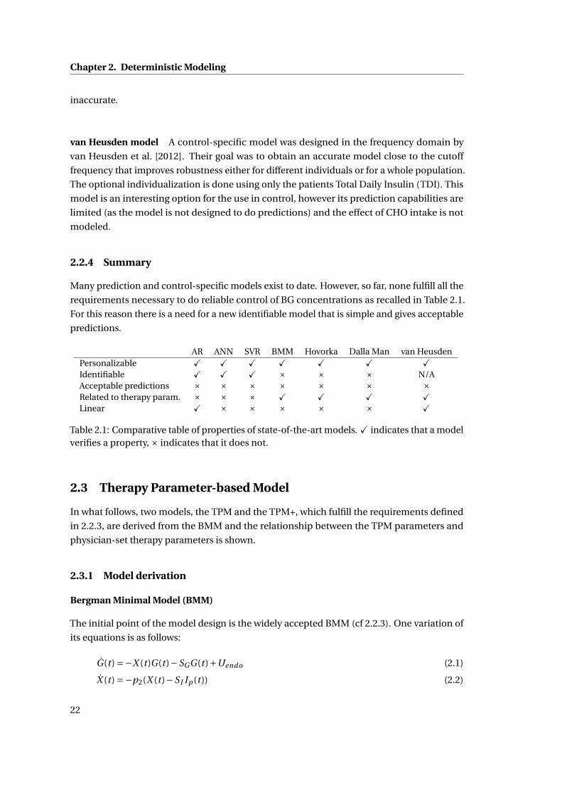
Chapter 2. Deterministic Modeling
inaccurate.
van Heusden model A control-specific model was designed in the frequency domain by
van Heusden et al. [2012]. Their goal was to obtain an accurate model close to the cutoff
frequency that improves robustness either for different individuals or for a whole population.
The optional individualization is done using only the patients Total Daily Insulin (TDI). This
model is an interesting option for the use in control, however its prediction capabilities are
limited (as the model is not designed to do predictions) and the effect of CHO intake is not
modeled.
2.2.4 Summary
Many prediction and control-specific models exist to date. However, so far, none fulfill all the
requirements necessary to do reliable control of BG concentrations as recalled in Table 2.1.
For this reason there is a need for a new identifiable model that is simple and gives acceptable
predictions.
AR ANN SVR BMM Hovorka Dalla Man van HeusdenPersonalizable X X X X X X XIdentifiable X X X × × × N/AAcceptable predictions × × × × × × ×Related to therapy param. × × × X X X XLinear X × × × × × X
Table 2.1: Comparative table of properties of state-of-the-art models. X indicates that a modelverifies a property, × indicates that it does not.
2.3 Therapy Parameter-based Model
In what follows, two models, the TPM and the TPM+, which fulfill the requirements defined
in 2.2.3, are derived from the BMM and the relationship between the TPM parameters and
physician-set therapy parameters is shown.
2.3.1 Model derivation
Bergman Minimal Model (BMM)
The initial point of the model design is the widely accepted BMM (cf 2.2.3). One variation of
its equations is as follows:
G(t ) =−X (t )G(t )−SGG(t )+Uendo (2.1)
X (t ) =−p2(X (t )−S I Ip (t )) (2.2)
22
2.3. Therapy Parameter-based Model
where G is the BG concentration in mg ·dl−1, X is the insulin action in mi n−1, SG is the
glucose effectiveness at zero insulin in mi n−1, S I is the insulin sensitivity in U−1 ·mi n−1 · l ,
Uendo is the endogenous glucose production in mg ·dl−1 ·mi n−1, and p2 is the inverse of the
time constant of the insulin action in mi n−1. Ip is the plasma insulin concentration in U /l .
To be used as a prediction model, the BMM needs to be extended with sub-models to account
for insulin absorption an CHO intake .
Minimal model (MM)
Prud’homme et al. [2011] recently extended the BMM by substituting the insulin action and
insulin absorption models by a 2nd -order insulin action model and by adding the 2nd -order
linear carbohydrates (CHO) sub-model by Hovorka et al. [2004], resulting in the following set
of ODEs:
G(t ) =−Kx X (t )G(t )−SGG(t )+Uendo +KgUG (t ) (2.3)
UG (t ) =−agUG (t )+agUG ,1(t ) (2.4)
UG ,1(t ) =−agUG ,1(t )+agUC HO(t ) (2.5)
X (t ) =−ax X (t )+ax X1(t ) (2.6)
X1(t ) =−ax X1(t )+axUI (t ) (2.7)
where the new states are the gut glucose absorption UG in g ·mi n−1, the intermediate gut
glucose absorption UG ,1 in g ·mi n−1, and the intermediate insulin action X1 in U ·mi n−1. X
is now given in U ·mi n−1. Additional model parameters are introduced: the meal sensitivity
Kg in mg ·dl−1 ·g−1, the inverse of the meal time constant ag in mi n−1, the insulin sensitivity
Kx in U−1 (different from S I ), and the inverse of the insulin absorption/action time constant
ax in mi n−1. The manipulated inputs are the subcutaneous insulin infusion, UI in U ·mi n−1
and the carbohydrate intake rate UC HO in g ·mi n−1. This model will be referred to as the
Minimal Model (MM) hereafter.
The fact that the insulin concentration - which is neither measured nor used - is not explicitly
modeled improves the identifiability of this model compared to models using the original
BMM insulin action of Equation (2.2).
However, the results presented by Prud’homme et al. [2011] show that, despite improved
identifiability and the use of prior knowledge, the resulting predictions are still unsatisfactory
and lead to sub-optimal insulin infusions. Another drawback of the MM lies in the behavior
induced by the bilinear term of Equation 2.3 (Equation 2.1 for the BMM). While according to
the term −Kx X (t)G(t), high BG values should lead to high insulin effect and vice-versa, the
opposite effect has been observed in practice (Unger and Grundy [1985]). Especially prolonged
hyperglycemia blunts the effect of insulin.
23
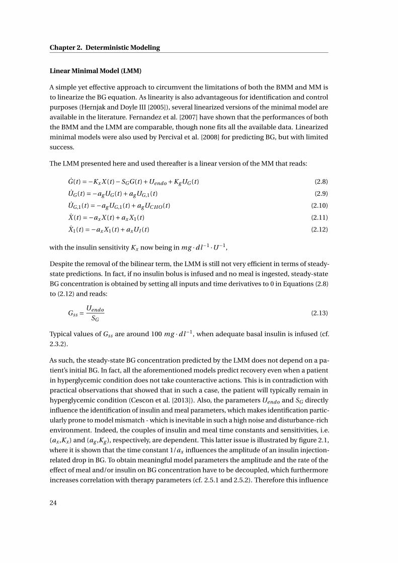
Chapter 2. Deterministic Modeling
Linear Minimal Model (LMM)
A simple yet effective approach to circumvent the limitations of both the BMM and MM is
to linearize the BG equation. As linearity is also advantageous for identification and control
purposes (Hernjak and Doyle III [2005]), several linearized versions of the minimal model are
available in the literature. Fernandez et al. [2007] have shown that the performances of both
the BMM and the LMM are comparable, though none fits all the available data. Linearized
minimal models were also used by Percival et al. [2008] for predicting BG, but with limited
success.
The LMM presented here and used thereafter is a linear version of the MM that reads:
G(t ) =−Kx X (t )−SGG(t )+Uendo +KgUG (t ) (2.8)
UG (t ) =−agUG (t )+agUG ,1(t ) (2.9)
UG ,1(t ) =−agUG ,1(t )+agUC HO(t ) (2.10)
X (t ) =−ax X (t )+ax X1(t ) (2.11)
X1(t ) =−ax X1(t )+axUI (t ) (2.12)
with the insulin sensitivity Kx now being in mg ·dl−1 ·U−1,
Despite the removal of the bilinear term, the LMM is still not very efficient in terms of steady-
state predictions. In fact, if no insulin bolus is infused and no meal is ingested, steady-state
BG concentration is obtained by setting all inputs and time derivatives to 0 in Equations (2.8)
to (2.12) and reads:
Gss = Uendo
SG(2.13)
Typical values of Gss are around 100 mg ·dl−1, when adequate basal insulin is infused (cf.
2.3.2).
As such, the steady-state BG concentration predicted by the LMM does not depend on a pa-
tient’s initial BG. In fact, all the aforementioned models predict recovery even when a patient
in hyperglycemic condition does not take counteractive actions. This is in contradiction with
practical observations that showed that in such a case, the patient will typically remain in
hyperglycemic condition (Cescon et al. [2013]). Also, the parameters Uendo and SG directly
influence the identification of insulin and meal parameters, which makes identification partic-
ularly prone to model mismatch - which is inevitable in such a high noise and disturbance-rich
environment. Indeed, the couples of insulin and meal time constants and sensitivities, i.e.
(ax ,Kx ) and (ag ,Kg ), respectively, are dependent. This latter issue is illustrated by figure 2.1,
where it is shown that the time constant 1/ax influences the amplitude of an insulin injection-
related drop in BG. To obtain meaningful model parameters the amplitude and the rate of the
effect of meal and/or insulin on BG concentration have to be decoupled, which furthermore
increases correlation with therapy parameters (cf. 2.5.1 and 2.5.2). Therefore this influence
24
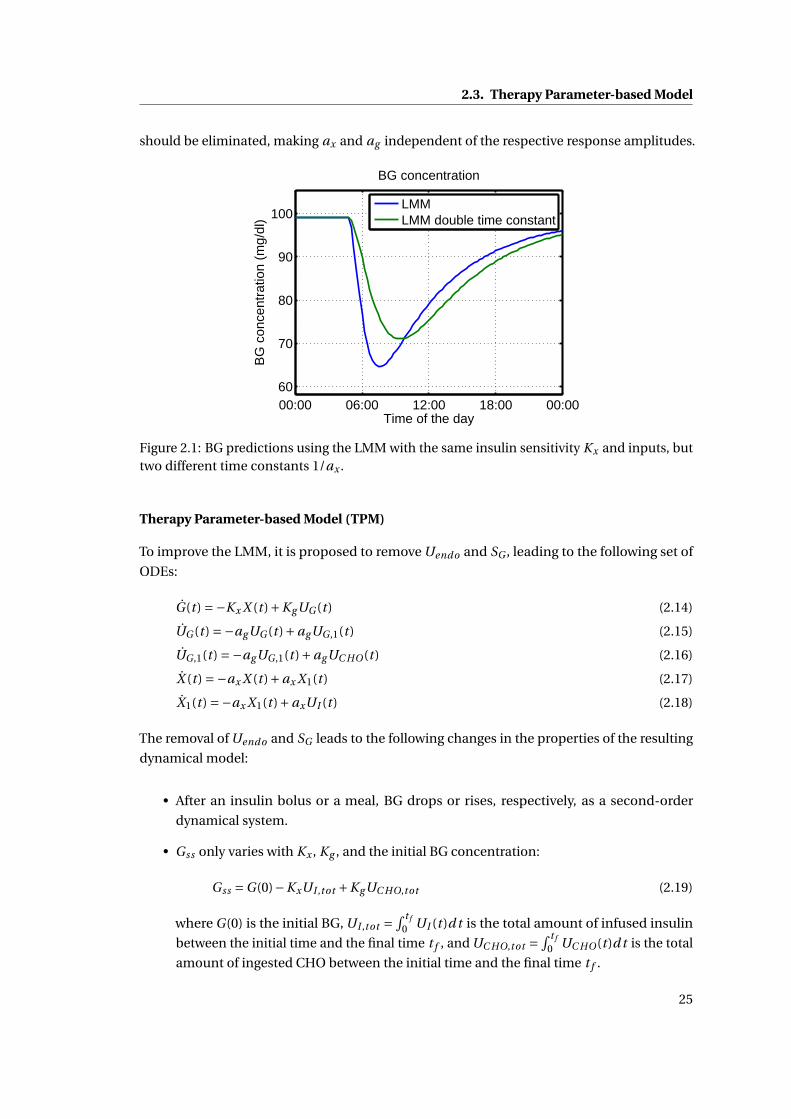
2.3. Therapy Parameter-based Model
should be eliminated, making ax and ag independent of the respective response amplitudes.
00:00 06:00 12:00 18:00 00:0060
70
80
90
100
Time of the day
BG
con
cent
ratio
n (m
g/dl
)
BG concentration
LMMLMM double time constant
Figure 2.1: BG predictions using the LMM with the same insulin sensitivity Kx and inputs, buttwo different time constants 1/ax .
Therapy Parameter-based Model (TPM)
To improve the LMM, it is proposed to remove Uendo and SG , leading to the following set of
ODEs:
G(t ) =−Kx X (t )+KgUG (t ) (2.14)
UG (t ) =−agUG (t )+agUG ,1(t ) (2.15)
UG ,1(t ) =−agUG ,1(t )+agUC HO(t ) (2.16)
X (t ) =−ax X (t )+ax X1(t ) (2.17)
X1(t ) =−ax X1(t )+axUI (t ) (2.18)
The removal of Uendo and SG leads to the following changes in the properties of the resulting
dynamical model:
• After an insulin bolus or a meal, BG drops or rises, respectively, as a second-order
dynamical system.
• Gss only varies with Kx , Kg , and the initial BG concentration:
Gss =G(0)−KxUI ,tot +KgUC HO,tot (2.19)
where G(0) is the initial BG, UI ,tot =∫ t f
0 UI (t)d t is the total amount of infused insulin
between the initial time and the final time t f , and UC HO,tot =∫ t f
0 UC HO(t )d t is the total
amount of ingested CHO between the initial time and the final time t f .
25
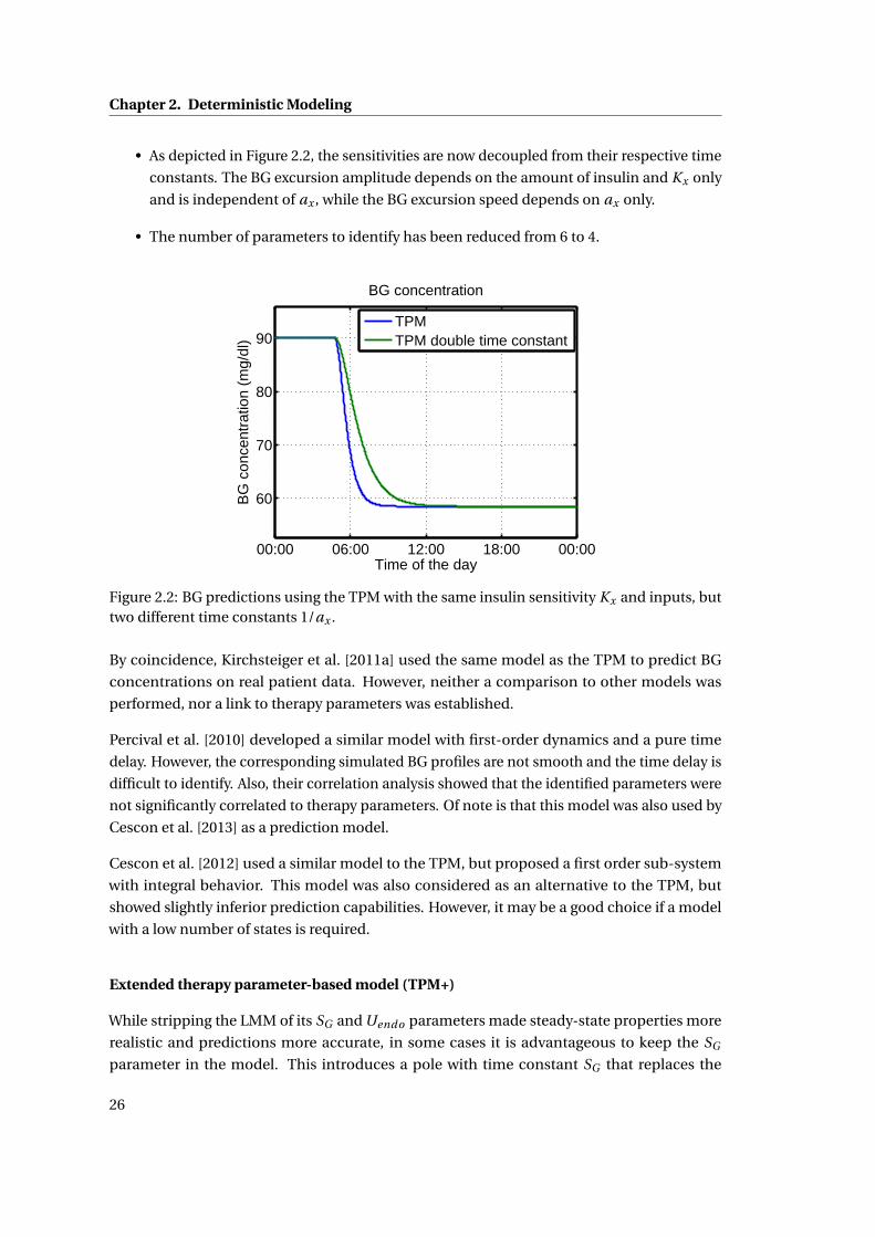
Chapter 2. Deterministic Modeling
• As depicted in Figure 2.2, the sensitivities are now decoupled from their respective time
constants. The BG excursion amplitude depends on the amount of insulin and Kx only
and is independent of ax , while the BG excursion speed depends on ax only.
• The number of parameters to identify has been reduced from 6 to 4.
00:00 06:00 12:00 18:00 00:00
60
70
80
90
Time of the day
BG
con
cent
ratio
n (m
g/dl
)
BG concentration
TPMTPM double time constant
Figure 2.2: BG predictions using the TPM with the same insulin sensitivity Kx and inputs, buttwo different time constants 1/ax .
By coincidence, Kirchsteiger et al. [2011a] used the same model as the TPM to predict BG
concentrations on real patient data. However, neither a comparison to other models was
performed, nor a link to therapy parameters was established.
Percival et al. [2010] developed a similar model with first-order dynamics and a pure time
delay. However, the corresponding simulated BG profiles are not smooth and the time delay is
difficult to identify. Also, their correlation analysis showed that the identified parameters were
not significantly correlated to therapy parameters. Of note is that this model was also used by
Cescon et al. [2013] as a prediction model.
Cescon et al. [2012] used a similar model to the TPM, but proposed a first order sub-system
with integral behavior. This model was also considered as an alternative to the TPM, but
showed slightly inferior prediction capabilities. However, it may be a good choice if a model
with a low number of states is required.
Extended therapy parameter-based model (TPM+)
While stripping the LMM of its SG and Uendo parameters made steady-state properties more
realistic and predictions more accurate, in some cases it is advantageous to keep the SG
parameter in the model. This introduces a pole with time constant SG that replaces the
26
2.3. Therapy Parameter-based Model
integrator of the TPM. This is consistent with the observation made by Cescon et al. [2013]
that the integral effect of the model by Percival et al. [2010] may be replaced by a very slow
pole.
The proposed model is given as
G(t ) =−Kx X (t )−SGG(t )+KgUG (t ) (2.20)
UG (t ) =−agUG (t )+agUG ,1(t ) (2.21)
UG ,1(t ) =−agUG ,1(t )+agUC HO(t ) (2.22)
X (t ) =−ax X (t )+ax X1(t ) (2.23)
X1(t ) =−ax X1(t )+axUI (t ) (2.24)
Two remarks are in order for frequently identified values of SG :
• SG = 0. In this case the TPM+ is the same as the TPM.
• SG very small. It can be derived from 2.13 that Gss is zero and hence BG always converges
to 0 mg/dl. This may be an unrealistic value, but as shown in 2.5.1 and 2.5.2, it is not
detrimental for diabetes treatment as it tends to underestimate BG concentration,
mostly leading to benign treatment decisions. The small value of SG guarantees a
relatively slow convergence to this value, such that therapy parameters may still be
identified and BG concentrations stay realistic on a moderate prediction horizon.
2.3.2 Standard therapy
In the following paragraphs, the principles of the standard bolus and insulin pump therapy
are described and it is shown how therapy parameters are related to the parameters of the
TPM and TPM+.
Standard therapy definition
Patients with T1DM:
• Take a SMBG measurement (Gm) before a meal, or whenever they suspect their BG to
be out of range,
• Compare Gm to the target BG (Gt ), and compute the difference: ∆G =Gm −Gt ,
• Compute the correction bolus as UI ,cor r =∆G/C F , with C F being the correction factor
in mg ·dl−1 ·U−1. Icor r may be negative if the patient plans to ingest a meal.
• Compute the meal bolus as UI ,meal = I 2C ·C HO, with I 2C being the insulin-to-carbohydrates
ratio in U · g−1, and C HO being the corresponding weight of carbohydrates in g .
27
Chapter 2. Deterministic Modeling
• Inject the bolus UI =UI ,cor r +UI ,meal using their insulin pump or pen.
Indeed, C F and I 2C correspond to the therapy parameters and are set by a physician. C F
quantifies the drop in BG resulting from a 1U insulin injection (U corresponds to the "insulin
unit", the international unit of insulin) at steady-state, while I 2C indicates how much insulin
should be injected per gram of ingested CHO. MS = I 2C ·C F can thus be defined as the meal
sensitivity, which indicates the increase in BG per gram of ingested carbohydrates.
From the viewpoint of systems theory, a way to interpret the standard therapy parameters MS
and C F is by assimilating them to the parameters of a static model, identified by physicians,
that maps the amount of insulin to the future steady-state BG.
Basal insulin
With an insulin pump, insulin may be infused almost continuously. This basal rate is useful
in that it counteracts circadian variations in insulin sensitivity, such as the dawn effect. It is
generally tuned by a physician in such a way that, in the absence of disturbances (such as
meals or physical activity), BG stays approximately at the target value throughout the day.
Hereafter, we will always assume a properly set basal rate. In this case, basal insulin is not
considered as an input, i.e. inputs correspond exclusively to insulin boluses.
The proper adjustment of the basal rate is all but trivial and requires an experienced physician
and lengthy patient observations. Currently, basal adjustments are also a field of research
with a strong impact on diabetes treatment, especially in the case of open-loop treatment. For
example methods such as run-to-run are proposed by Palerm et al. [2008].
Relation between therapy parameters and the TPM
Proposition 1. The TPM parameter Kx is equal to the therapy parameter C F .
Proof. If a 1U insulin bolus is infused at t = 0, UI (s) = 1 and, in the absence of previous insulin
boluses and meals, C F , according to the definition given in 2.3.2, is given as:
C F =−(G(∞)−G(0)) (2.25)
where G(∞) is the BG at steady-state and G(0) the initial BG.
Using the Laplace transform of the TPM equations 2.14, 2.17, and 2.18:
G(s) =− Kx
s(1+ 1
axs)2 UI (s)+ 1
sG(0) (2.26)
28
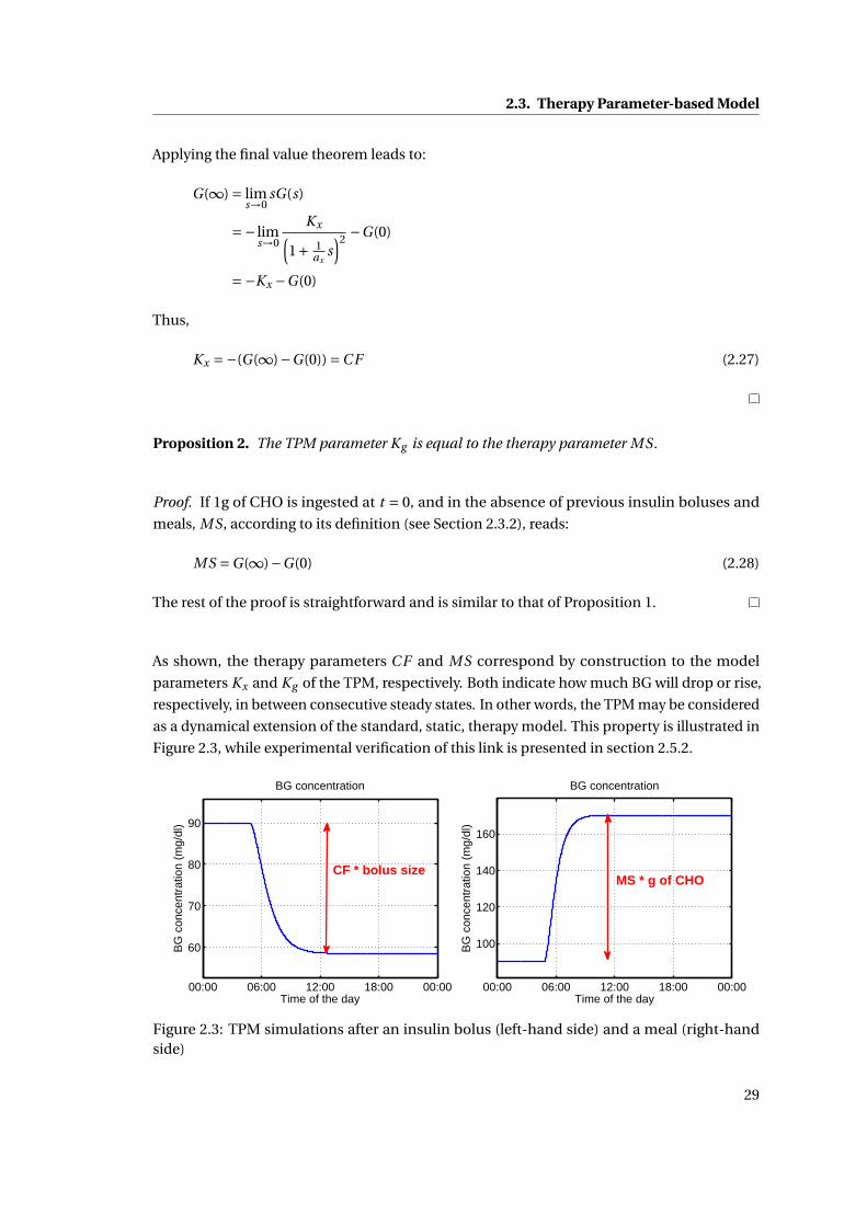
2.3. Therapy Parameter-based Model
Applying the final value theorem leads to:
G(∞) = lims→0
sG(s)
=− lims→0
Kx(1+ 1
axs)2 −G(0)
=−Kx −G(0)
Thus,
Kx =−(G(∞)−G(0)) =C F (2.27)
Proposition 2. The TPM parameter Kg is equal to the therapy parameter MS.
Proof. If 1g of CHO is ingested at t = 0, and in the absence of previous insulin boluses and
meals, MS, according to its definition (see Section 2.3.2), reads:
MS =G(∞)−G(0) (2.28)
The rest of the proof is straightforward and is similar to that of Proposition 1.
As shown, the therapy parameters C F and MS correspond by construction to the model
parameters Kx and Kg of the TPM, respectively. Both indicate how much BG will drop or rise,
respectively, in between consecutive steady states. In other words, the TPM may be considered
as a dynamical extension of the standard, static, therapy model. This property is illustrated in
Figure 2.3, while experimental verification of this link is presented in section 2.5.2.
00:00 06:00 12:00 18:00 00:00
60
70
80
90
Time of the day
BG
con
cent
ratio
n (m
g/dl
)
BG concentration
CF * bolus size
00:00 06:00 12:00 18:00 00:00
100
120
140
160
Time of the day
BG
con
cent
ratio
n (m
g/dl
)
BG concentration
MS * g of CHO
Figure 2.3: TPM simulations after an insulin bolus (left-hand side) and a meal (right-handside)
29
Chapter 2. Deterministic Modeling
The link between therapy and model parameters is very valuable, because TPM parameters
have a physical meaning that is recognized by physicians and may therefore be accepted more
easily. On the other hand, a priori knowledge of the physician-set therapy parameters can be
used, if available, to improve the reliability of the TPM parameters.
The relation between therapy parameters and TPM+ parameters cannot be shown in the
general case. In the case where SG equals zero, the TPM+ is equal to the TPM and the two
propositions hold. However, in the opposite, this cannot be verified, but the fact that TPM+
properties are very close to those of the TPM as long as SG is small explains a good correlation
with therapy parameters as shown in 2.5.1 and 2.5.2.
2.4 Validation Tools and Methods
This section describes the data used for the validation of the TPM and TPM+ as well as the
practical methods and tools.
2.4.1 Validation data
Data from two different sources is used:
• Simulated BG profiles generated with the UVa simulator show how the proposed models
perform on this widely accepted tool. More details concerning the UVa simulator are
given in appendix A.1 and the 4 day nominal scenario specified in A.1.1 is used for
cross-validation. The noiseless measurements of the 10 adults are used and are sampled
with a period of 15 minutes.
• Data from 10 of the 12 patients from the clinical study described in appendix A.2 are
used to validate the TPM and the TPM+ on real patient data.
2.4.2 Identification method
Model parameters identification is performed by minimizing the following weighted least
squares objective function J :
J (θ) =D∑
d=1αd Jd (θ) (2.29)
where θ is the vector of model parameters to estimate (θ = [ax ag Kx Kg ]T for the TPM, e.g.), D
is the number of days, αd is the weight associated to day d , and Jd is defined for each day d :
Jd (θ) =Nd∑i=1
(Gd ,i −Gd ,i (θ))2 (2.30)
30
2.4. Validation Tools and Methods
where Nd is the number of BG measurements for day d , Gd ,i and Gd ,i are the measured and
simulated BG concentrations on day d , respectively.
The optimal values θ∗ are such that they minimize the cumulated (and weighted) prediction
error:
minθ
J (θ) =D∑
d=1
(αd
(Nd∑i=1
(Gd ,i −Gd ,i (θ))2
))(2.31)
s.t. Model Equations (2.32)
where the Model Equations (Equations (2.14)-(2.18) for the TPM, e.g.) are integrated to
compute the predicted values Gd ,i (θ) at the sampling instant i of day d under the same
conditions than the corresponding measured values Gd ,i , for any choice of θ.
2.4.3 Reliable insulin action
Particular attention has to be paid to the estimation of insulin action, as, for instance, underes-
timating the insulin effect increases the risk of overdosing insulin. It is made more complicated
when meals and insulin boluses are taken simultaneously, since the effects of carbohydrates
and insulin cancel each other out, especially if they act at similar speeds. Note that this remark
further justifies the choice of slow meals in the context of the clinical study associated with
this thesis, as the meals taken by the subjects were mostly slower than the insulin actions.
This difficulty to identify insulin parameters - worsened by the high noise level - is depicted
in Figure 2.4. It is shown that when the meal and the bolus are taken simultaneously, the
simulated BG does not change significantly when Kx is doubled, while the right-hand side
plot shows the large sensitivity of the simulated BG profile to a change in Kx when the meal
and the bolus are taken separately. In other words, Figure 2.4 illustrates how difficult it is
to reliably identify Kx on the basis of BG measurements if the meal and the bolus are taken
simultaneously. Indeed, in such a case, it is possible to estimate the ratioKg
Kxthat corresponds
to I 2C , but not Kx (corresponding to C F ). This difficulty was also discussed by Finan et al.
[2007].
To circumvent this problem, the only solution is to perform insulin sensitivity tests, where a
bolus without a corresponding meal is infused.
2.4.4 Choice of metrics
In this validation, we propose to assess the quality of the LMM, the MM and the TPM by three
different indicators, Mean Absolute Difference (MAD), coefficient of determination (R2), and
Error Grid Analysis (EGA), which are detailed in the appendix B.
31
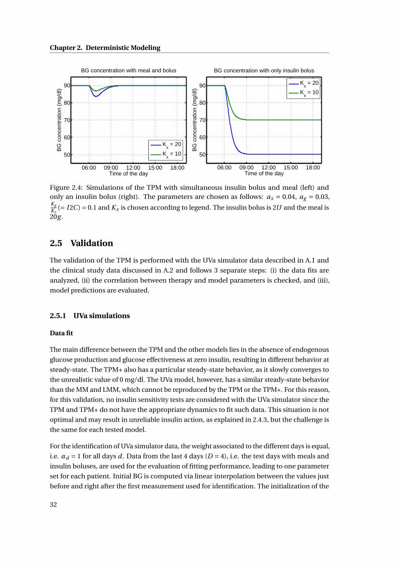
Chapter 2. Deterministic Modeling
06:00 09:00 12:00 15:00 18:00
50
60
70
80
90
Time of the day
BG
con
cent
ratio
n (m
g/dl
)
BG concentration with meal and bolus
Kx = 20
Kx = 10
06:00 09:00 12:00 15:00 18:00
50
60
70
80
90
Time of the day
BG
con
cent
ratio
n (m
g/dl
)
BG concentration with only insulin bolus
Kx = 20
Kx = 10
Figure 2.4: Simulations of the TPM with simultaneous insulin bolus and meal (left) andonly an insulin bolus (right). The parameters are chosen as follows: ax = 0.04, ag = 0.03,Kg
Kx(= I 2C ) = 0.1 and Kx is chosen according to legend. The insulin bolus is 2U and the meal is
20g .
2.5 Validation
The validation of the TPM is performed with the UVa simulator data described in A.1 and
the clinical study data discussed in A.2 and follows 3 separate steps: (i) the data fits are
analyzed, (ii) the correlation between therapy and model parameters is checked, and (iii),
model predictions are evaluated.
2.5.1 UVa simulations
Data fit
The main difference between the TPM and the other models lies in the absence of endogenous
glucose production and glucose effectiveness at zero insulin, resulting in different behavior at
steady-state. The TPM+ also has a particular steady-state behavior, as it slowly converges to
the unrealistic value of 0 mg/dl. The UVa model, however, has a similar steady-state behavior
than the MM and LMM, which cannot be reproduced by the TPM or the TPM+. For this reason,
for this validation, no insulin sensitivity tests are considered with the UVa simulator since the
TPM and TPM+ do not have the appropriate dynamics to fit such data. This situation is not
optimal and may result in unreliable insulin action, as explained in 2.4.3, but the challenge is
the same for each tested model.
For the identification of UVa simulator data, the weight associated to the different days is equal,
i.e. αd = 1 for all days d . Data from the last 4 days (D = 4), i.e. the test days with meals and
insulin boluses, are used for the evaluation of fitting performance, leading to one parameter
set for each patient. Initial BG is computed via linear interpolation between the values just
before and right after the first measurement used for identification. The initialization of the
32
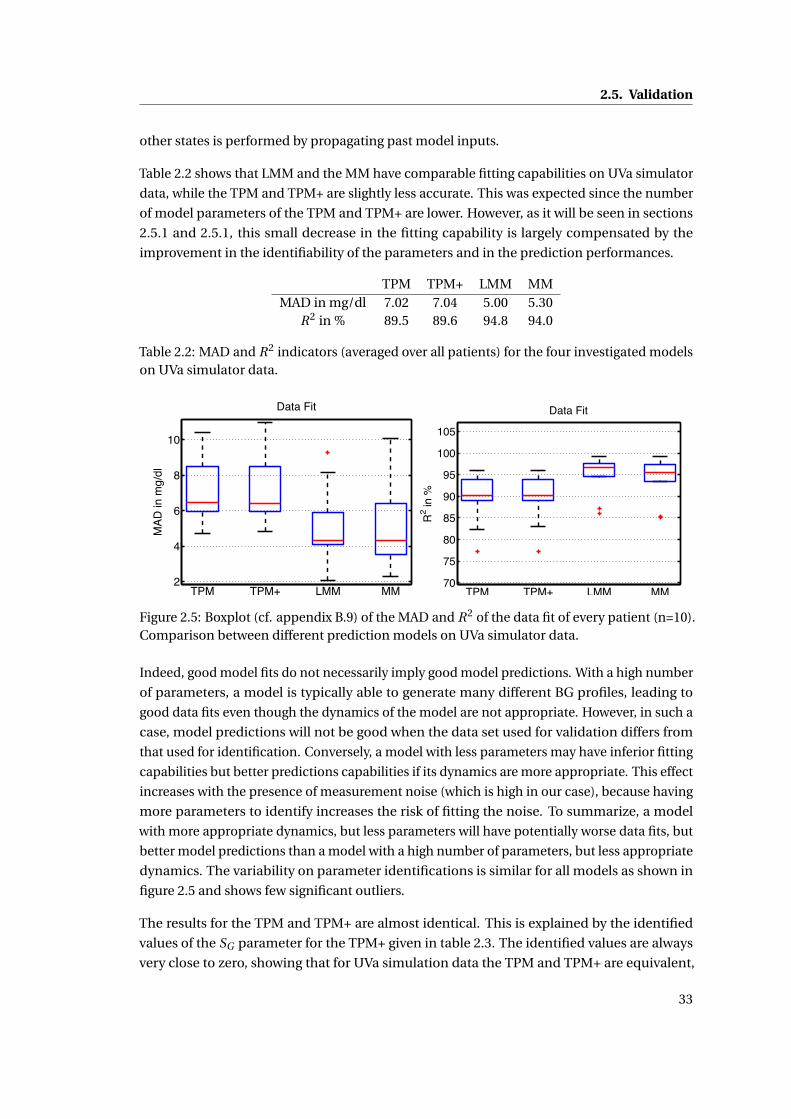
2.5. Validation
other states is performed by propagating past model inputs.
Table 2.2 shows that LMM and the MM have comparable fitting capabilities on UVa simulator
data, while the TPM and TPM+ are slightly less accurate. This was expected since the number
of model parameters of the TPM and TPM+ are lower. However, as it will be seen in sections
2.5.1 and 2.5.1, this small decrease in the fitting capability is largely compensated by the
improvement in the identifiability of the parameters and in the prediction performances.
TPM TPM+ LMM MMMAD in mg/dl 7.02 7.04 5.00 5.30
R2 in % 89.5 89.6 94.8 94.0
Table 2.2: MAD and R2 indicators (averaged over all patients) for the four investigated modelson UVa simulator data.
2
4
6
8
10
TPM TPM+ LMM MM
Data Fit
MAD
in m
g/dl
70
75
80
85
90
95
100
105
TPM TPM+ LMM MM
Data FitR
2 in %
Figure 2.5: Boxplot (cf. appendix B.9) of the MAD and R2 of the data fit of every patient (n=10).Comparison between different prediction models on UVa simulator data.
Indeed, good model fits do not necessarily imply good model predictions. With a high number
of parameters, a model is typically able to generate many different BG profiles, leading to
good data fits even though the dynamics of the model are not appropriate. However, in such a
case, model predictions will not be good when the data set used for validation differs from
that used for identification. Conversely, a model with less parameters may have inferior fitting
capabilities but better predictions capabilities if its dynamics are more appropriate. This effect
increases with the presence of measurement noise (which is high in our case), because having
more parameters to identify increases the risk of fitting the noise. To summarize, a model
with more appropriate dynamics, but less parameters will have potentially worse data fits, but
better model predictions than a model with a high number of parameters, but less appropriate
dynamics. The variability on parameter identifications is similar for all models as shown in
figure 2.5 and shows few significant outliers.
The results for the TPM and TPM+ are almost identical. This is explained by the identified
values of the SG parameter for the TPM+ given in table 2.3. The identified values are always
very close to zero, showing that for UVa simulation data the TPM and TPM+ are equivalent,
33
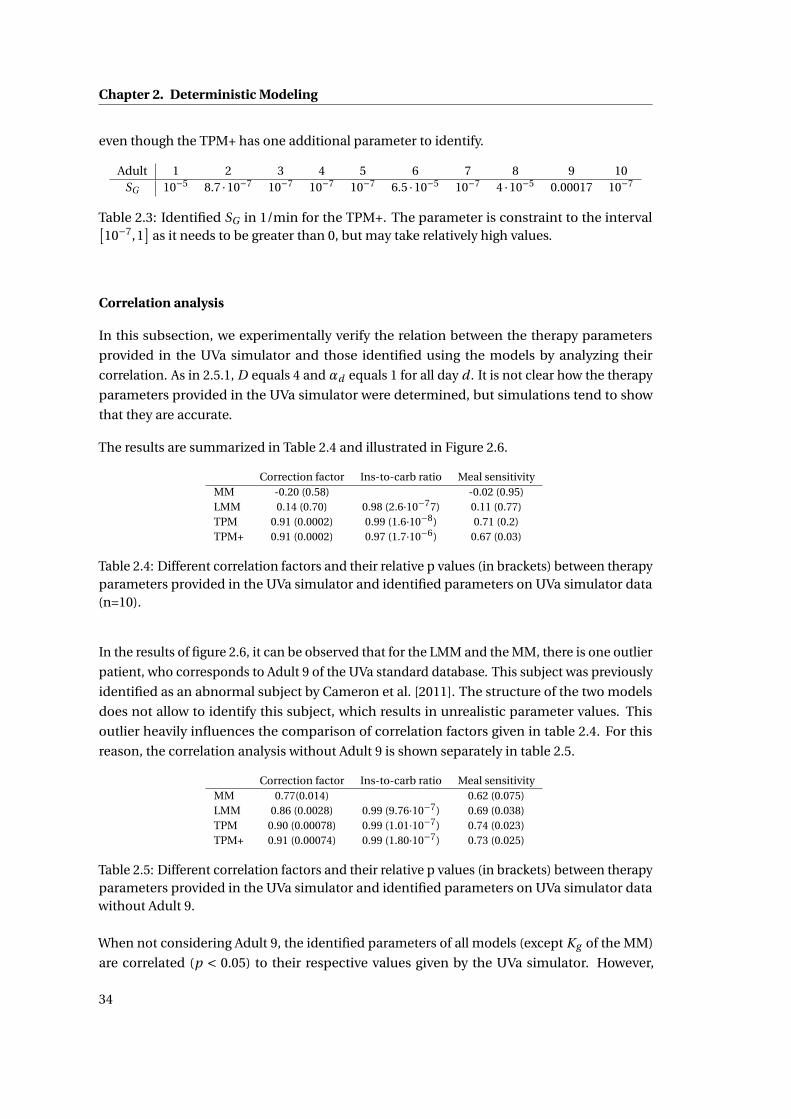
Chapter 2. Deterministic Modeling
even though the TPM+ has one additional parameter to identify.
Adult 1 2 3 4 5 6 7 8 9 10SG 10−5 8.7 ·10−7 10−7 10−7 10−7 6.5 ·10−5 10−7 4 ·10−5 0.00017 10−7
Table 2.3: Identified SG in 1/min for the TPM+. The parameter is constraint to the interval[10−7,1
]as it needs to be greater than 0, but may take relatively high values.
Correlation analysis
In this subsection, we experimentally verify the relation between the therapy parameters
provided in the UVa simulator and those identified using the models by analyzing their
correlation. As in 2.5.1, D equals 4 and αd equals 1 for all day d . It is not clear how the therapy
parameters provided in the UVa simulator were determined, but simulations tend to show
that they are accurate.
The results are summarized in Table 2.4 and illustrated in Figure 2.6.
Correction factor Ins-to-carb ratio Meal sensitivityMM -0.20 (0.58) -0.02 (0.95)LMM 0.14 (0.70) 0.98 (2.6·10−77) 0.11 (0.77)TPM 0.91 (0.0002) 0.99 (1.6·10−8) 0.71 (0.2)TPM+ 0.91 (0.0002) 0.97 (1.7·10−6) 0.67 (0.03)
Table 2.4: Different correlation factors and their relative p values (in brackets) between therapyparameters provided in the UVa simulator and identified parameters on UVa simulator data(n=10).
In the results of figure 2.6, it can be observed that for the LMM and the MM, there is one outlier
patient, who corresponds to Adult 9 of the UVa standard database. This subject was previously
identified as an abnormal subject by Cameron et al. [2011]. The structure of the two models
does not allow to identify this subject, which results in unrealistic parameter values. This
outlier heavily influences the comparison of correlation factors given in table 2.4. For this
reason, the correlation analysis without Adult 9 is shown separately in table 2.5.
Correction factor Ins-to-carb ratio Meal sensitivityMM 0.77(0.014) 0.62 (0.075)LMM 0.86 (0.0028) 0.99 (9.76·10−7) 0.69 (0.038)TPM 0.90 (0.00078) 0.99 (1.01·10−7) 0.74 (0.023)TPM+ 0.91 (0.00074) 0.99 (1.80·10−7) 0.73 (0.025)
Table 2.5: Different correlation factors and their relative p values (in brackets) between therapyparameters provided in the UVa simulator and identified parameters on UVa simulator datawithout Adult 9.
When not considering Adult 9, the identified parameters of all models (except Kg of the MM)
are correlated (p < 0.05) to their respective values given by the UVa simulator. However,
34
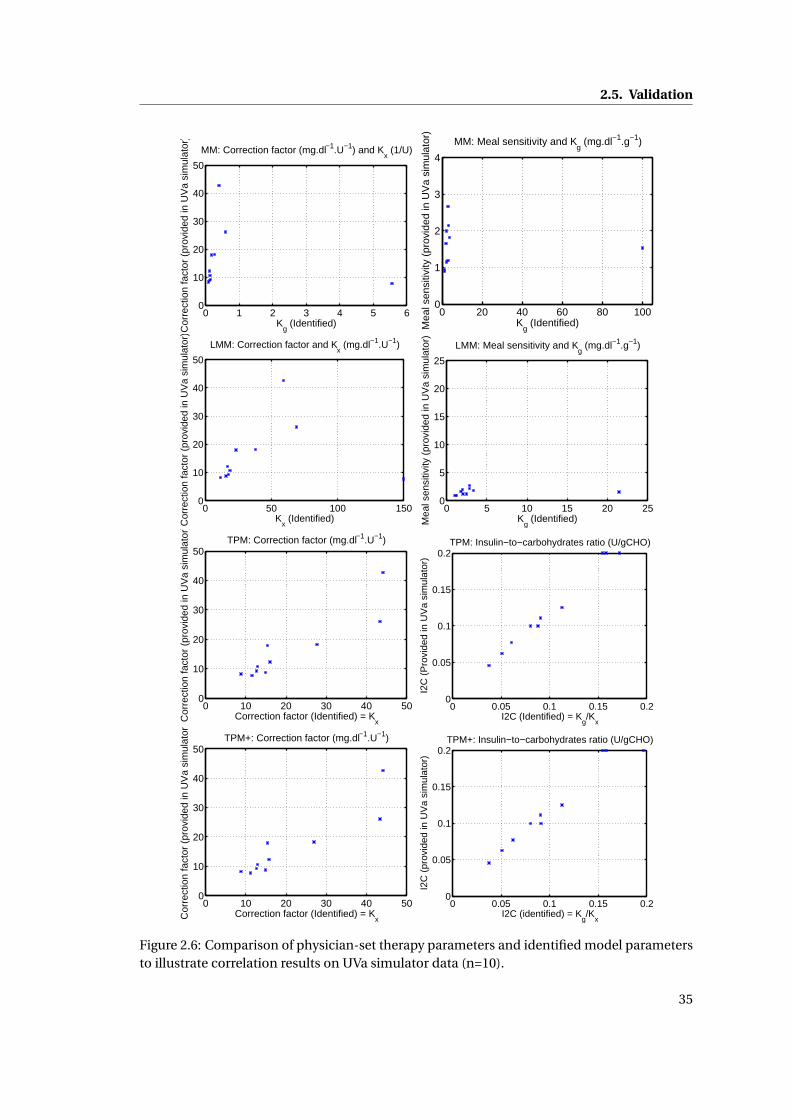
2.5. Validation
0 1 2 3 4 5 60
10
20
30
40
50
MM: Correction factor (mg.dl−1.U−1) and Kx (1/U)
Kg (Identified)
Cor
rect
ion
fact
or (
prov
ided
in U
Va
sim
ulat
or)
0 20 40 60 80 1000
1
2
3
4
MM: Meal sensitivity and Kg (mg.dl−1.g−1)
Kg (Identified)M
eal s
ensi
tivity
(pr
ovid
ed in
UV
a si
mul
ator
)
0 50 100 1500
10
20
30
40
50
LMM: Correction factor and Kx (mg.dl−1.U−1)
Kx (Identified)C
orre
ctio
n fa
ctor
(pr
ovid
ed in
UV
a si
mul
ator
)
0 5 10 15 20 250
5
10
15
20
25
LMM: Meal sensitivity and Kg (mg.dl−1.g−1)
Kg (Identified)M
eal s
ensi
tivity
(pr
ovid
ed in
UV
a si
mul
ator
)
0 10 20 30 40 500
10
20
30
40
50TPM: Correction factor (mg.dl−1.U−1)
Correction factor (Identified) = KxC
orre
ctio
n fa
ctor
(pr
ovid
ed in
UV
a si
mul
ator
)
0 0.05 0.1 0.15 0.20
0.05
0.1
0.15
0.2TPM: Insulin−to−carbohydrates ratio (U/gCHO)
I2C (Identified) = Kg/K
x
I2C
(P
rovi
ded
in U
Va
sim
ulat
or)
0 10 20 30 40 500
10
20
30
40
50TPM+: Correction factor (mg.dl−1.U−1)
Correction factor (Identified) = KxC
orre
ctio
n fa
ctor
(pr
ovid
ed in
UV
a si
mul
ator
)
0 0.05 0.1 0.15 0.20
0.05
0.1
0.15
0.2TPM+: Insulin−to−carbohydrates ratio (U/gCHO)
I2C (identified) = Kg/K
x
I2C
(pr
ovid
ed in
UV
a si
mul
ator
)
Figure 2.6: Comparison of physician-set therapy parameters and identified model parametersto illustrate correlation results on UVa simulator data (n=10).
35
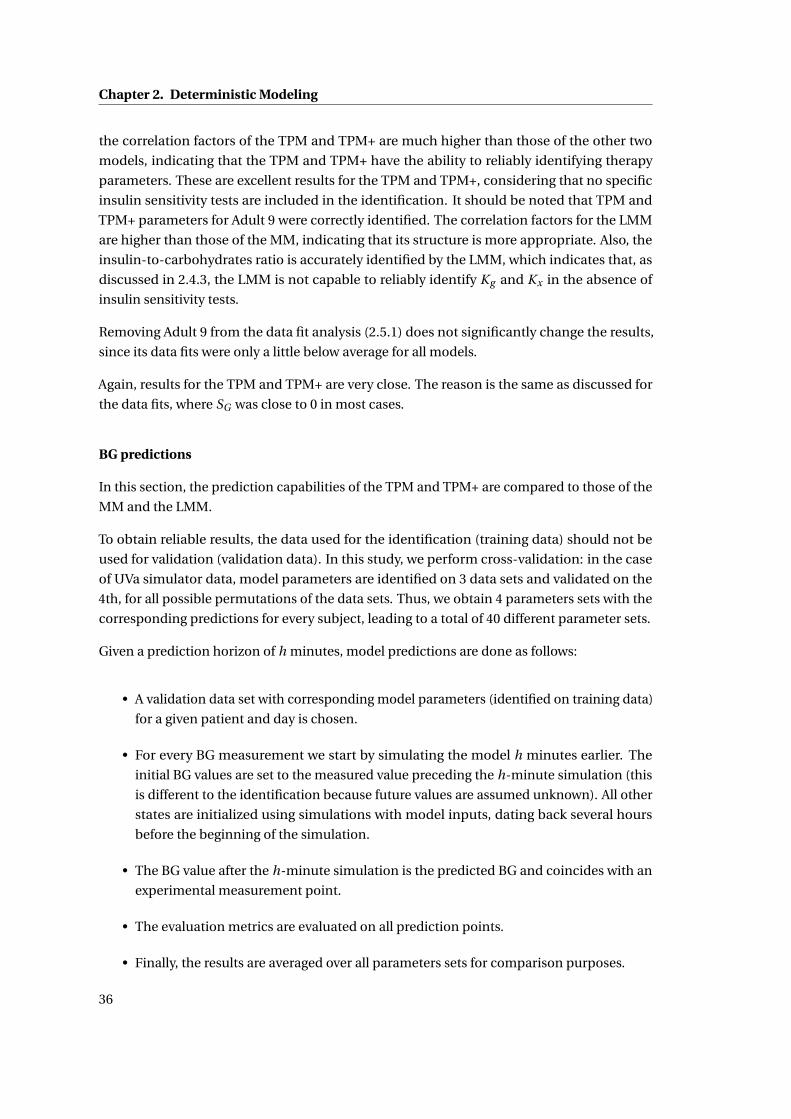
Chapter 2. Deterministic Modeling
the correlation factors of the TPM and TPM+ are much higher than those of the other two
models, indicating that the TPM and TPM+ have the ability to reliably identifying therapy
parameters. These are excellent results for the TPM and TPM+, considering that no specific
insulin sensitivity tests are included in the identification. It should be noted that TPM and
TPM+ parameters for Adult 9 were correctly identified. The correlation factors for the LMM
are higher than those of the MM, indicating that its structure is more appropriate. Also, the
insulin-to-carbohydrates ratio is accurately identified by the LMM, which indicates that, as
discussed in 2.4.3, the LMM is not capable to reliably identify Kg and Kx in the absence of
insulin sensitivity tests.
Removing Adult 9 from the data fit analysis (2.5.1) does not significantly change the results,
since its data fits were only a little below average for all models.
Again, results for the TPM and TPM+ are very close. The reason is the same as discussed for
the data fits, where SG was close to 0 in most cases.
BG predictions
In this section, the prediction capabilities of the TPM and TPM+ are compared to those of the
MM and the LMM.
To obtain reliable results, the data used for the identification (training data) should not be
used for validation (validation data). In this study, we perform cross-validation: in the case
of UVa simulator data, model parameters are identified on 3 data sets and validated on the
4th, for all possible permutations of the data sets. Thus, we obtain 4 parameters sets with the
corresponding predictions for every subject, leading to a total of 40 different parameter sets.
Given a prediction horizon of h minutes, model predictions are done as follows:
• A validation data set with corresponding model parameters (identified on training data)
for a given patient and day is chosen.
• For every BG measurement we start by simulating the model h minutes earlier. The
initial BG values are set to the measured value preceding the h-minute simulation (this
is different to the identification because future values are assumed unknown). All other
states are initialized using simulations with model inputs, dating back several hours
before the beginning of the simulation.
• The BG value after the h-minute simulation is the predicted BG and coincides with an
experimental measurement point.
• The evaluation metrics are evaluated on all prediction points.
• Finally, the results are averaged over all parameters sets for comparison purposes.
36
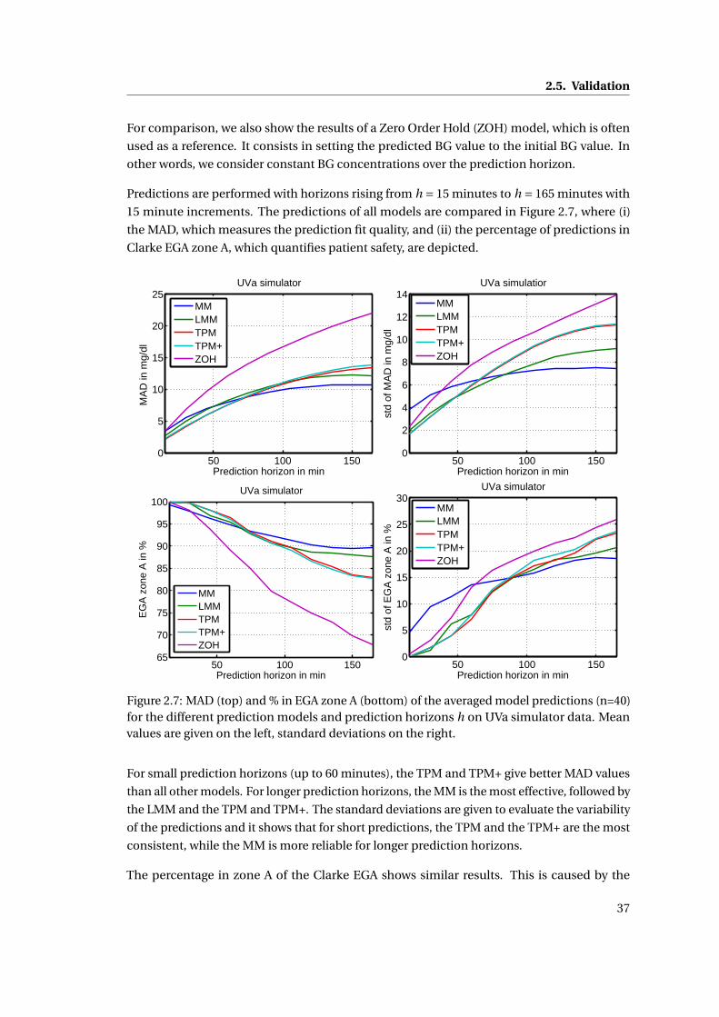
2.5. Validation
For comparison, we also show the results of a Zero Order Hold (ZOH) model, which is often
used as a reference. It consists in setting the predicted BG value to the initial BG value. In
other words, we consider constant BG concentrations over the prediction horizon.
Predictions are performed with horizons rising from h = 15 minutes to h = 165 minutes with
15 minute increments. The predictions of all models are compared in Figure 2.7, where (i)
the MAD, which measures the prediction fit quality, and (ii) the percentage of predictions in
Clarke EGA zone A, which quantifies patient safety, are depicted.
50 100 1500
5
10
15
20
25
Prediction horizon in min
MA
D in
mg/
dl
UVa simulator
MMLMMTPMTPM+ZOH
50 100 1500
2
4
6
8
10
12
14
Prediction horizon in min
std
of M
AD
in m
g/dl
UVa simulatior
MMLMMTPMTPM+ZOH
50 100 15065
70
75
80
85
90
95
100
Prediction horizon in min
EG
A z
one
A in
%
UVa simulator
MMLMMTPMTPM+ZOH
50 100 1500
5
10
15
20
25
30
Prediction horizon in min
std
of E
GA
zon
e A
in %
UVa simulator
MMLMMTPMTPM+ZOH
Figure 2.7: MAD (top) and % in EGA zone A (bottom) of the averaged model predictions (n=40)for the different prediction models and prediction horizons h on UVa simulator data. Meanvalues are given on the left, standard deviations on the right.
For small prediction horizons (up to 60 minutes), the TPM and TPM+ give better MAD values
than all other models. For longer prediction horizons, the MM is the most effective, followed by
the LMM and the TPM and TPM+. The standard deviations are given to evaluate the variability
of the predictions and it shows that for short predictions, the TPM and the TPM+ are the most
consistent, while the MM is more reliable for longer prediction horizons.
The percentage in zone A of the Clarke EGA shows similar results. This is caused by the
37
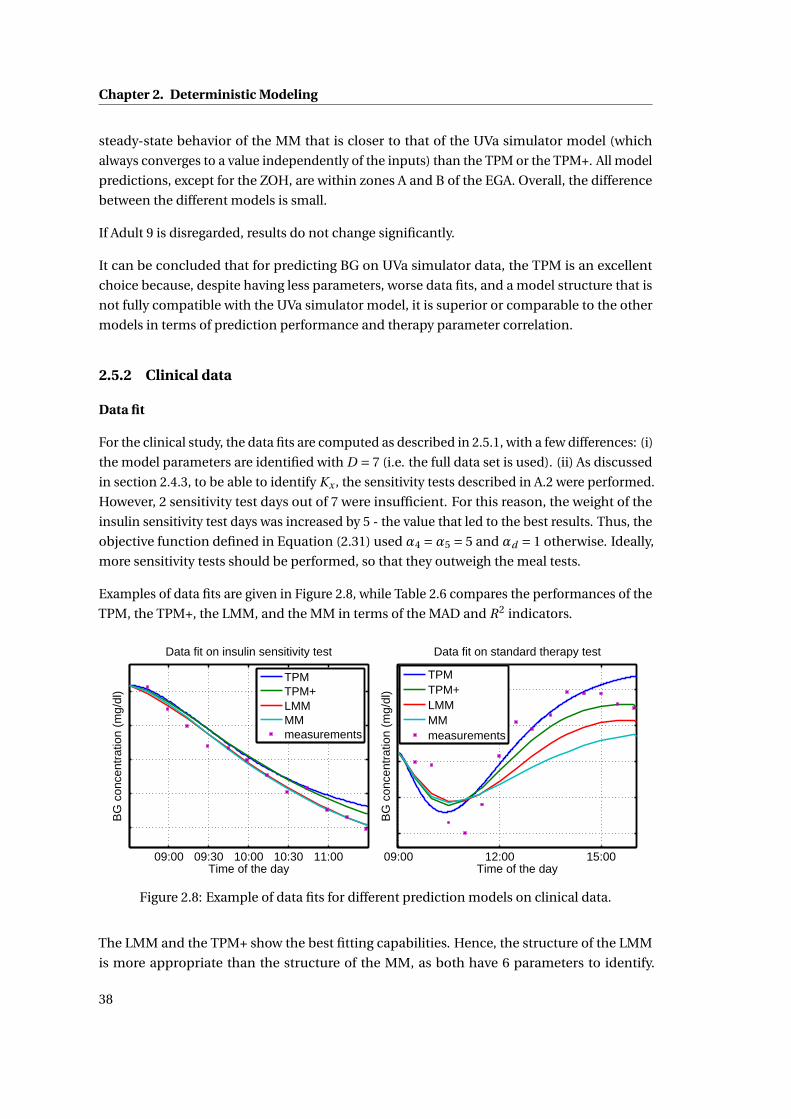
Chapter 2. Deterministic Modeling
steady-state behavior of the MM that is closer to that of the UVa simulator model (which
always converges to a value independently of the inputs) than the TPM or the TPM+. All model
predictions, except for the ZOH, are within zones A and B of the EGA. Overall, the difference
between the different models is small.
If Adult 9 is disregarded, results do not change significantly.
It can be concluded that for predicting BG on UVa simulator data, the TPM is an excellent
choice because, despite having less parameters, worse data fits, and a model structure that is
not fully compatible with the UVa simulator model, it is superior or comparable to the other
models in terms of prediction performance and therapy parameter correlation.
2.5.2 Clinical data
Data fit
For the clinical study, the data fits are computed as described in 2.5.1, with a few differences: (i)
the model parameters are identified with D = 7 (i.e. the full data set is used). (ii) As discussed
in section 2.4.3, to be able to identify Kx , the sensitivity tests described in A.2 were performed.
However, 2 sensitivity test days out of 7 were insufficient. For this reason, the weight of the
insulin sensitivity test days was increased by 5 - the value that led to the best results. Thus, the
objective function defined in Equation (2.31) used α4 =α5 = 5 and αd = 1 otherwise. Ideally,
more sensitivity tests should be performed, so that they outweigh the meal tests.
Examples of data fits are given in Figure 2.8, while Table 2.6 compares the performances of the
TPM, the TPM+, the LMM, and the MM in terms of the MAD and R2 indicators.
09:00 09:30 10:00 10:30 11:00Time of the day
BG
con
cent
ratio
n (m
g/dl
)
Data fit on insulin sensitivity test
TPMTPM+LMMMMmeasurements
09:00 12:00 15:00Time of the day
BG
con
cent
ratio
n (m
g/dl
)
Data fit on standard therapy test
TPMTPM+LMMMMmeasurements
Figure 2.8: Example of data fits for different prediction models on clinical data.
The LMM and the TPM+ show the best fitting capabilities. Hence, the structure of the LMM
is more appropriate than the structure of the MM, as both have 6 parameters to identify.
38
2.5. Validation
TPM TPM+ LMM MMMAD in mg/dl 12.89 10.90 10.56 12.09
R2 in % 72.42 80.76 81.16 76.15
Table 2.6: MAD and R2 indicators (averaged over all patients) for the four investigated modelson clinical data.
However, the TPM+, with only 5 parameters to identify, has almost the same fitting capabilities
than the LMM and should therefore be preferred. The performances of the TPM and the MM
are comparable, with a slight advantage for the MM. Figure 2.9 depicts the variability of data
fits, that is the lowest for the LMM and the TPM+ and increases for the MM and the TPM. A
higher variability is due to a higher number of patients that were more difficult to fit. However,
it will be seen in sections 2.5.2 and 2.5.2 that this is not detrimental neither to parameter
identification nor to model prediction, the reason being that some patients have intrinsically
higher variability in their BG concentrations.
8
10
12
14
16
18
20
22
TPM TPM+ LMM MM
Data Fit
MAD
in m
g/dl
50
60
70
80
90
TPM TPM+ LMM MM
Data Fit
R2 in
%
Figure 2.9: Boxplot (cf. appendix B.9) of the MAD and R2 of the data fit of every patient (n=10).Comparison between different prediction models on clinical data.
While identifying the LMM, for 4 patients out of 10, the values of SG and Uendo collapsed to 0,
with the consequence that the LMM becomes identical to the TPM and that the corresponding
model fits are very close. A similar observation is made for the TPM+, where the SG parameter
converges to 0 for 3 out of 10 patients, as shown in table 2.7.
Patient 1 2 3 4 5 6 7 9 11 12SG 0.0007 10−7 0.00003 10−7 0.0006 10−7 0.0008 0.0017 0.0006 0.0010
Table 2.7: Identified SG in 1/min for the TPM+. The parameter is constraint to the interval[10−7,1
].
39
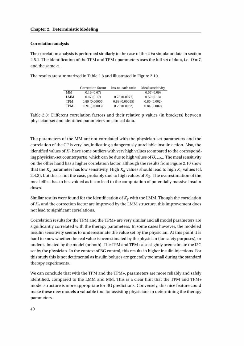
Chapter 2. Deterministic Modeling
Correlation analysis
The correlation analysis is performed similarly to the case of the UVa simulator data in section
2.5.1. The identification of the TPM and TPM+ parameters uses the full set of data, i.e. D = 7,
and the same α.
The results are summarized in Table 2.8 and illustrated in Figure 2.10.
Correction factor Ins-to-carb ratio Meal sensitivityMM 0.16 (0.67) 0.57 (0.09)LMM 0.47 (0.17) 0.78 (0.0077) 0.52 (0.13)TPM 0.89 (0.00055) 0.89 (0.00055) 0.85 (0.002)TPM+ 0.91 (0.0003) 0.79 (0.0062) 0.84 (0.002)
Table 2.8: Different correlation factors and their relative p values (in brackets) betweenphysician-set and identified parameters on clinical data.
The parameters of the MM are not correlated with the physician-set parameters and the
correlation of the CF is very low, indicating a dangerously unreliable insulin action. Also, the
identified values of Kx have some outliers with very high values (compared to the correspond-
ing physician-set counterparts), which can be due to high values of Uendo . The meal sensitivity
on the other hand has a higher correlation factor, although the results from Figure 2.10 show
that the Kg parameter has low sensitivity. High Kg values should lead to high Kx values (cf.
2.4.3), but this is not the case, probably due to high values of SG . The overestimation of the
meal effect has to be avoided as it can lead to the computation of potentially massive insulin
doses.
Similar results were found for the identification of Kg with the LMM. Though the correlation
of Kx and the correction factor are improved by the LMM structure, this improvement does
not lead to significant correlations.
Correlation results for the TPM and the TPM+ are very similar and all model parameters are
significantly correlated with the therapy parameters. In some cases however, the modeled
insulin sensitivity seems to underestimate the value set by the physician. At this point it is
hard to know whether the real value is overestimated by the physician (for safety purposes), or
underestimated by the model (or both). The TPM and TPM+ also slightly overestimate the I2C
set by the physician. In the context of BG control, this results in higher insulin injections. For
this study this is not detrimental as insulin boluses are generally too small during the standard
therapy experiments.
We can conclude that with the TPM and the TPM+, parameters are more reliably and safely
identified, compared to the LMM and MM. This is a clear hint that the TPM and TPM+
model structure is more appropriate for BG predictions. Conversely, this nice feature could
make these new models a valuable tool for assisting physicians in determining the therapy
parameters.
40
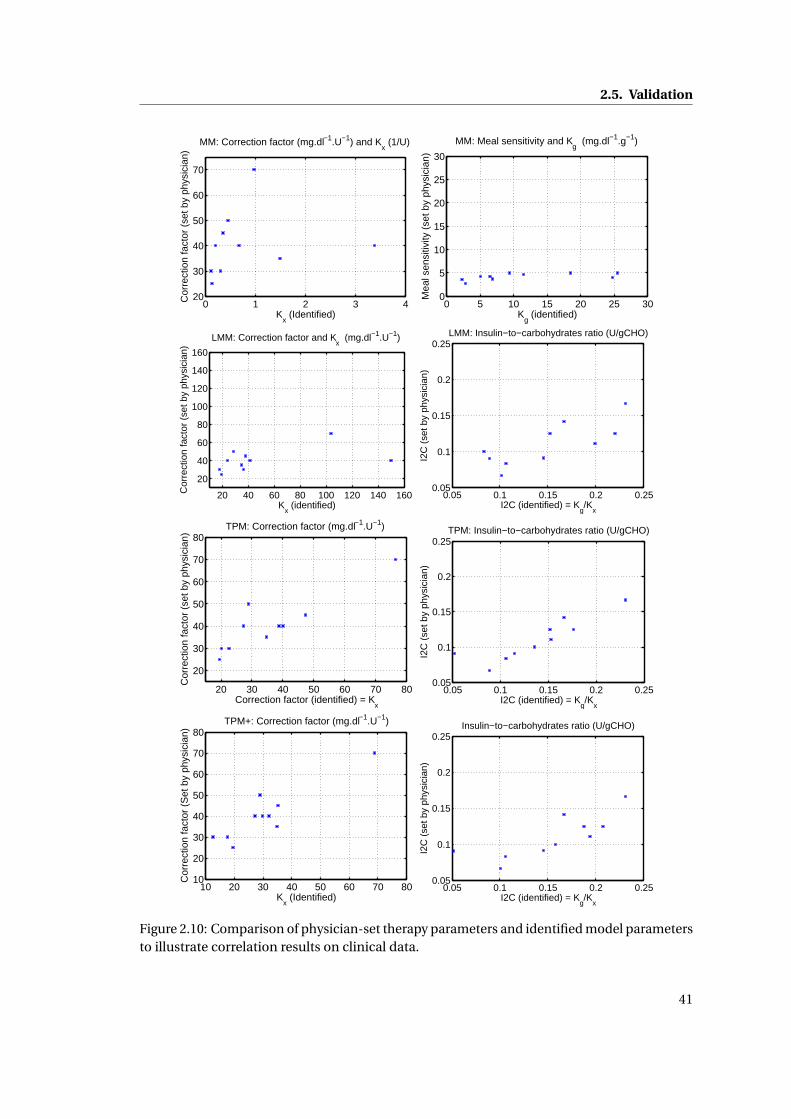
2.5. Validation
0 1 2 3 420
30
40
50
60
70
MM: Correction factor (mg.dl−1.U−1) and Kx (1/U)
Kx (Identified)
Cor
rect
ion
fact
or (
set b
y ph
ysic
ian)
0 5 10 15 20 25 300
5
10
15
20
25
30
MM: Meal sensitivity and Kg (mg.dl−1.g−1)
Kg (identified)
Mea
l sen
sitiv
ity (
set b
y ph
ysic
ian)
20 40 60 80 100 120 140 160
20
40
60
80
100
120
140
160
LMM: Correction factor and Kx (mg.dl−1.U−1)
Kx (identified)
Cor
rect
ion
fact
or (
set b
y ph
ysic
ian)
0.05 0.1 0.15 0.2 0.250.05
0.1
0.15
0.2
0.25LMM: Insulin−to−carbohydrates ratio (U/gCHO)
I2C (identified) = Kg/K
x
I2C
(se
t by
phys
icia
n)
20 30 40 50 60 70 80
20
30
40
50
60
70
80TPM: Correction factor (mg.dl−1.U−1)
Correction factor (identified) = Kx
Cor
rect
ion
fact
or (
set b
y ph
ysic
ian)
0.05 0.1 0.15 0.2 0.250.05
0.1
0.15
0.2
0.25TPM: Insulin−to−carbohydrates ratio (U/gCHO)
I2C (identified) = Kg/K
x
I2C
(se
t by
phys
icia
n)
10 20 30 40 50 60 70 8010
20
30
40
50
60
70
80TPM+: Correction factor (mg.dl−1.U−1)
Kx (Identified)
Cor
rect
ion
fact
or (
Set
by
phys
icia
n)
0.05 0.1 0.15 0.2 0.250.05
0.1
0.15
0.2
0.25Insulin−to−carbohydrates ratio (U/gCHO)
I2C (identified) = Kg/K
x
I2C
(se
t by
phys
icia
n)
Figure 2.10: Comparison of physician-set therapy parameters and identified model parametersto illustrate correlation results on clinical data.
41
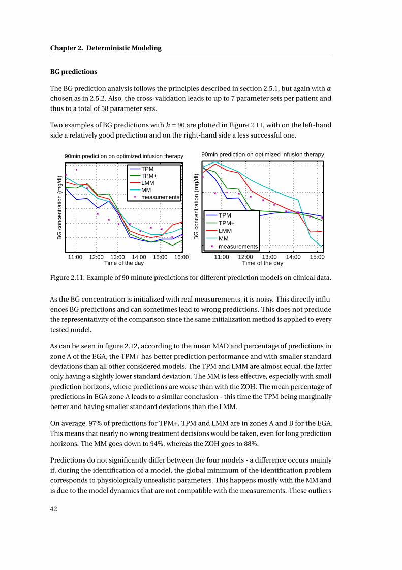
Chapter 2. Deterministic Modeling
BG predictions
The BG prediction analysis follows the principles described in section 2.5.1, but again with α
chosen as in 2.5.2. Also, the cross-validation leads to up to 7 parameter sets per patient and
thus to a total of 58 parameter sets.
Two examples of BG predictions with h = 90 are plotted in Figure 2.11, with on the left-hand
side a relatively good prediction and on the right-hand side a less successful one.
11:00 12:00 13:00 14:00 15:00 16:00Time of the day
BG
con
cent
ratio
n (m
g/dl
)
90min prediction on optimized infusion therapy
TPMTPM+LMMMMmeasurements
11:00 12:00 13:00 14:00 15:00Time of the day
BG
con
cent
ratio
n (m
g/dl
)
90min prediction on optimized infusion therapy
TPMTPM+LMMMMmeasurements
Figure 2.11: Example of 90 minute predictions for different prediction models on clinical data.
As the BG concentration is initialized with real measurements, it is noisy. This directly influ-
ences BG predictions and can sometimes lead to wrong predictions. This does not preclude
the representativity of the comparison since the same initialization method is applied to every
tested model.
As can be seen in figure 2.12, according to the mean MAD and percentage of predictions in
zone A of the EGA, the TPM+ has better prediction performance and with smaller standard
deviations than all other considered models. The TPM and LMM are almost equal, the latter
only having a slightly lower standard deviation. The MM is less effective, especially with small
prediction horizons, where predictions are worse than with the ZOH. The mean percentage of
predictions in EGA zone A leads to a similar conclusion - this time the TPM being marginally
better and having smaller standard deviations than the LMM.
On average, 97% of predictions for TPM+, TPM and LMM are in zones A and B for the EGA.
This means that nearly no wrong treatment decisions would be taken, even for long prediction
horizons. The MM goes down to 94%, whereas the ZOH goes to 88%.
Predictions do not significantly differ between the four models - a difference occurs mainly
if, during the identification of a model, the global minimum of the identification problem
corresponds to physiologically unrealistic parameters. This happens mostly with the MM and
is due to the model dynamics that are not compatible with the measurements. These outliers
42
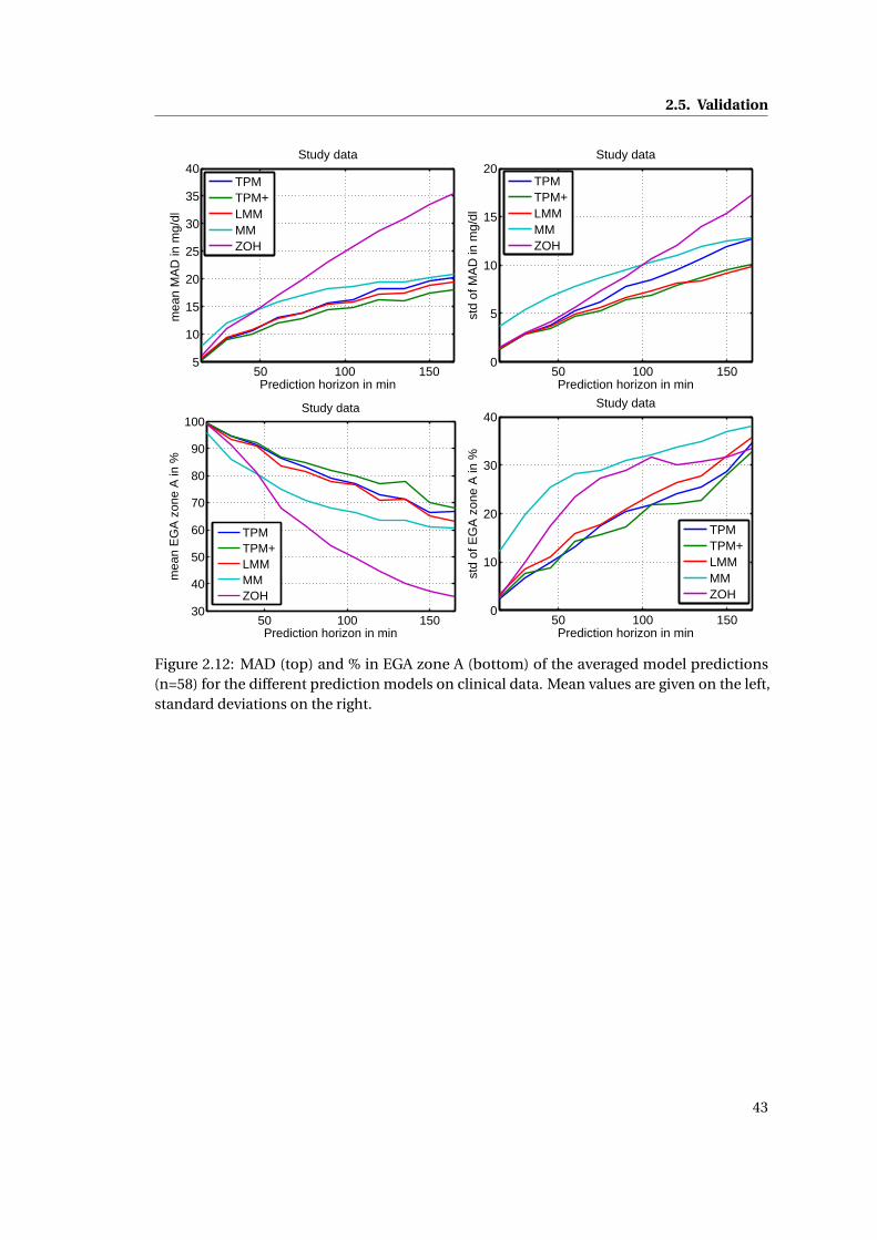
2.5. Validation
50 100 1505
10
15
20
25
30
35
40
Prediction horizon in min
mea
n M
AD
in m
g/dl
Study data
TPMTPM+LMMMMZOH
50 100 1500
5
10
15
20
Prediction horizon in min
std
of M
AD
in m
g/dl
Study data
TPMTPM+LMMMMZOH
50 100 15030
40
50
60
70
80
90
100
Prediction horizon in min
mea
n E
GA
zon
e A
in %
Study data
TPMTPM+LMMMMZOH
50 100 1500
10
20
30
40
Prediction horizon in min
std
of E
GA
zon
e A
in %
Study data
TPMTPM+LMMMMZOH
Figure 2.12: MAD (top) and % in EGA zone A (bottom) of the averaged model predictions(n=58) for the different prediction models on clinical data. Mean values are given on the left,standard deviations on the right.
43
Chapter 2. Deterministic Modeling
result in worse average performance outcomes and are the main reason for the differences
between the different models in figure 2.12.
Overall, the TPM always shows superior or comparable prediction capabilities. This is particu-
larly interesting considering that only 4 parameters have to be identified. This compensates
for the slightly inferior fitting capabilities. The TPM+ on the other hand is superior to all other
tested models, but has 5 parameters to identify. Hence the TPM+ should be preferred for long
prediction horizons, while the TPM is the model of choice if computational resources are
scarce or prediction horizons are shorter.
As a concluding remark, it should be noted that the different days of the clinical study were
very similar, which most likely makes predicting BG easier. With more varied scenarios, some
of the tested models could prove inappropriate. It would therefore be interesting to test the
model in a more diverse setting, similar to the analysis on the UVa simulator data, however
this is not possible with the currently available data.
2.5.3 Comparison of results of the UVa simulator data and clinical data
The results obtained with the UVa simulator data and clinical data are consistent. Because
of improved BG predictions, parameter correlation, and the reduced number of parameters,
the TPM is the best choice on UVa simulator data and clinical data, while the TPM+ should
be preferred for long-horizon predictions for real patients. Another main difference between
results on the UVa simulator data and clinical data is the relative performance of the LMM
and the MM: LMM is better on clinical data, while the MM is better on UVa simulator data.
This is probably due to the fact that the MM dynamics are closer to the UVa simulator and to
its non-linearities, while the LMM dynamics are closer to real human glucose dynamics.
2.6 Conclusion
The TPM and the TPM+ measure up to the expectations of being reliable but simple prediction
models identifiable on BG measurements only. Stripping the models to a bare minimum (they
can hardly be any simpler) allows reliable parameter identification, even in the presence of the
characteristic high noise levels in BG measurements. We linked the model parameters directly
to physician-set therapy parameters and showed their strong correlation. This adds another
safety layer to the resulting model identification and the model may easily be personalized.
As expected, model fits were slightly worse than with other models - a result of the lower
number of parameters. However, model predictions were on par or better than the alternatives.
A higher number of parameters is therefore not necessary.
Predictions are used to calculate insulin doses and as such are critical for patient safety. If
carefully identified, the TPM and the TPM+ lead to reliable insulin sensitivity estimation, which
is rarely the case with the other models (identified under the same conditions). Additionally,
44
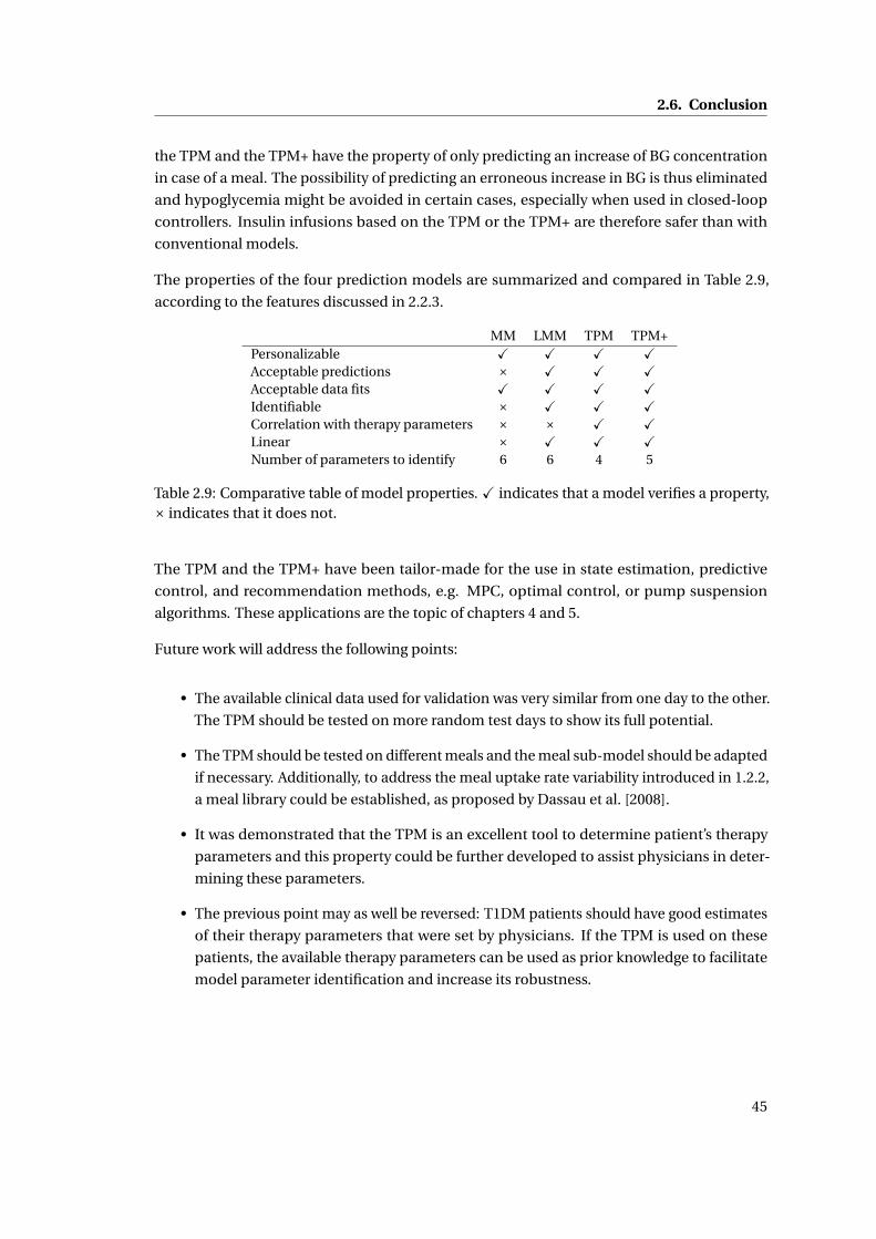
2.6. Conclusion
the TPM and the TPM+ have the property of only predicting an increase of BG concentration
in case of a meal. The possibility of predicting an erroneous increase in BG is thus eliminated
and hypoglycemia might be avoided in certain cases, especially when used in closed-loop
controllers. Insulin infusions based on the TPM or the TPM+ are therefore safer than with
conventional models.
The properties of the four prediction models are summarized and compared in Table 2.9,
according to the features discussed in 2.2.3.
MM LMM TPM TPM+Personalizable X X X XAcceptable predictions × X X XAcceptable data fits X X X XIdentifiable × X X XCorrelation with therapy parameters × × X XLinear × X X XNumber of parameters to identify 6 6 4 5
Table 2.9: Comparative table of model properties. X indicates that a model verifies a property,× indicates that it does not.
The TPM and the TPM+ have been tailor-made for the use in state estimation, predictive
control, and recommendation methods, e.g. MPC, optimal control, or pump suspension
algorithms. These applications are the topic of chapters 4 and 5.
Future work will address the following points:
• The available clinical data used for validation was very similar from one day to the other.
The TPM should be tested on more random test days to show its full potential.
• The TPM should be tested on different meals and the meal sub-model should be adapted
if necessary. Additionally, to address the meal uptake rate variability introduced in 1.2.2,
a meal library could be established, as proposed by Dassau et al. [2008].
• It was demonstrated that the TPM is an excellent tool to determine patient’s therapy
parameters and this property could be further developed to assist physicians in deter-
mining these parameters.
• The previous point may as well be reversed: T1DM patients should have good estimates
of their therapy parameters that were set by physicians. If the TPM is used on these
patients, the available therapy parameters can be used as prior knowledge to facilitate
model parameter identification and increase its robustness.
45

3 Stochastic Modeling
3.1 Introduction
In chapter 2, many of the challenges identified in section 1.2 are addressed and overcome.
However, the large uncertainty described in section 1.2.2 makes accurate BG predictions
difficult and requires a probabilistic approach.
Inter-patient variability is taken into account by identifying individual model parameters for
each patient. However, this requires models with very specific properties such as the TPM.
Meal uptake rate variability can be addressed by identifying model parameters for different
types of meals and constructing a meal library (Dassau et al. [2008], Prud’homme et al. [2011]).
However, methods to quantify intra-patient variability are more difficult and rarely found in
the literature. Such methods aim to find confidence intervals on predicted BG concentrations.
One possibility to address this problem is by applying modal interval analysis (García-Jaramillo
et al. [2012], Gardeñes et al. [2001]), which leads to models computing the upper and lower
limits on BG, based on any deterministic model and on model parameter bounds. This
method is computationally efficient, but difficult to set up. Additionally, no experimental
verification, nor method to determine parameter intervals is given. Kirchsteiger et al. [2011b]
addressed the problem in a similar way by computing upper and lower bounds, based on TPM
parameter identification. Another approach is to add process noise to transform Ordinary
Differential Equations (ODEs) into Stochastic Differential Equations (SDEs) and to identify
the process noise amplitude as proposed by Klim [2009]. However, finding this amplitude is
not straightforward. A similar approach by Cameron [2010] uses a multi-model method, but is
computationally demanding. Finally, it is also possible to estimate uncertainties using linear
regression prediction methods. However, according to Cameron et al. [2008], this method is
only reliable for short prediction horizons of up to 20 minutes .
In this chapter a complete procedure to estimate the quality of BG predictions as a function
of time by constructing a stochastic model and quantifying model uncertainties is proposed.
The ODEs of a well-chosen continuous and deterministic model are transformed into SDEs
by adding parametric uncertainties. Model parameter uncertainties are estimated during
47
Chapter 3. Stochastic Modeling
standard parameter identification and, as a consequence, no additional parameters need to
be identified. The uncertainties are propagated using EKF theory.
This chapter is structured as follows: first, in section 3.2, the stochastic model, the uncertainty
estimation, and the covariance propagation are introduced. Then, in section 3.3 and the
proposed method is applied to the TPM. In section 3.4, predictions using the newly designed
sTPM are done and validated using simulated and clinical data. Finally, conclusions are drawn
and future work is proposed in section 3.6.
3.2 Stochastic modeling
3.2.1 Construction of a stochastic model
The construction of a stochastic model is based on a well-chosen deterministic model. The
latter one should be continuous and expressed as:
x(t ) = fdet(x(t ),u(t ),θθθ
), (3.1)
where x is the vector of n states, t is the time, u is the m-dimension input vector, θθθ is a
vector containing p model parameters, and fdet is a differentiable function that defines
the model dynamics. In this chapter only, vectors and matrices are represented in bold.
One of the states in x should be the BG concentration. If this model is well chosen, it gives
appropriate BG predictions. Nevertheless, because of the random nature of human glycemia,
these predictions will rarely be accurate and a stochastic model is useful to evaluate the quality
of the deterministic predictions. For this reason, it is useful to turn the deterministic model
into a stochastic one of the form
x(t ) = fsto(x(t ),u(t ),w(t ),θθθ
), (3.2)
where w(t ) ∼N (0,Q), Q is the covariance matrix of a multivariate zero-mean Gaussian, and
fsto is a differentiable function that defines the model dynamics. Now x(t ) is a random variable
whose distribution is analyzed and propagated through time.
The biggest challenge in estimating the quality of BG predictions is to model how the uncer-
tainty w(t) affects the BG concentration. Often a zero-mean univariate Gaussian is added
to the BG state and all other states remain unchanged Klim [2009]. It is difficult to choose
a numerical value for this Gaussian’s standard deviation σ and it requires additional and
computationally important identification steps. Moreover, with this approach, the uncertainty
is independent of model inputs, even though meal inputs are a more important source of
uncertainty than insulin injections, for example.
In order to define a meaningful and easy-to-identify alternative, it is proposed to consider
the parametric uncertainty of the model parameters. So, to obtain a stochastic model, θθθ is
48
3.2. Stochastic modeling
replaced by a normally distributed parameter vectorΘΘΘ in equation 3.1, defined as
ΘΘΘ∼N (θθθ,Q) (3.3)
∼θθθ+w(t ) (3.4)
In other words, a Gaussian term is added to every parameterΘi , such thatΘi = θi +wi , where
w =[
w1 . . . wp
]Thas the covariance matrix Q. Thus the uncertainty on several parame-
ters can be correlated. The strong assumption that the parameters are normally distributed
presents the biggest drawback of the proposed method, as physiological parameters are often
found to be log-normally distributed Zhang and Popp [1994]. However, as shown in section
3.4, results are convincing.
If the deterministic model is linear with respect to its parameters, equation 3.2 can be written
as
dx(t ) = fdet(x(t ),u(t ),θθθ
)d t + g
(x(t ),u(t ),θθθ
)dw(t ) (3.5)
where w is a standard Brownian motion vector of dimension p and covariance matrix Q, and
g is a deterministic function. fdet is called the drift function and quantifies the deterministic
part of the model, same as in equation 3.1. g is called diffusive function and quantifies the
uncertainty of the different states.
To simulate the stochastic model, the Euler-Maruyama scheme can be used, for instance. The
simulations could then be used for different Monte Carlo methods. These have the advantage
of giving accurate results, but at a high computational price.
3.2.2 Propagating uncertainties
If the complete distribution of the states is not necessarily needed, but the propagation
of its variance is sufficient, the computational burden of Monte Carlo simulations can be
considerably alleviated by propagating the covariance using EKF theory (Simon [2006]). The
model designed in the previous section is not forcibly linear. In the case of non-linearities,
finding the evolution of the states and its uncertainties needs the application of a non-linear
version of the KF. For this reason, the model is linearized along the estimated trajectory and A
and L are defined:
A(t ) = ∂ fsto(t )
∂x(t )
∣∣∣∣x(t ),w0
(3.6)
and
L(t ) = ∂ fsto(t )
∂w(t )
∣∣∣∣x(t ),w0
, (3.7)
49
Chapter 3. Stochastic Modeling
where x(t ) is the estimated state vector x(t ) at time t . The estimated trajectory has no process
noise, hence w0 = 0. Furthermore,
Q(t ) = L(t )QL(t )T . (3.8)
The state estimation is the same as for the deterministic model and the state covariance P(t )
propagates over time, giving the following set of equations to integrate:
˙x(t ) = fsto(x(t ),u(t ),w0,θθθ
)(3.9)
P(t ) = A(t )P(t )+P(t )A(t )T + Q(t ), (3.10)
where w0 = 0. The initial conditions for x(t ) are set using BG measurements and state propa-
gation using past inputs, while the initial conditions for P(t) are determined by covariance
propagation using past inputs.
Using the covariance matrix, the standard deviation on the BG state can be isolated and
thus, its uncertainty estimated at every point in time. Furthermore, the distribution of the
uncertainty of the states over time is assumed to follow a normal distribution. This is a strong
assumption, but allows computing confidence intervals on BG concentration. It might not
hold for models with strong non-linearities, nevertheless, if the model is linear and linearly
parameterized, this is not an approximation and exact results are found.
The 95% confidence interval is defined by
P (xBG (t )−1.96σBG (t ) ≤ xBG (t ) ≤ xBG (t )+1.96σBG (t )) = 0.95, (3.11)
where xBG is the estimated BG state and σBG is the standard deviation of xBG . σBG =pPBG ,
where PBG is the variance of xBG , whose value is found on the BG element of the diagonal of
P. The upper 95% confidence limit is thus xBG (t )+1.96σBG (t ) and the lower one is xBG (t )−1.96σBG (t ).
In order to compute the confidence intervals, n(n+1)2 additional differential equations need to
be integrated. Including the n equations from the deterministic model, a total of n(n+3)2 ODEs
need to be integrated over the desired time horizon.
3.2.3 Parameter identification
The performance of the proposed stochastic model depends largely on the quality of the
estimated parameter vector θθθ and its covariance matrix Q. The following paragraphs show
how to find them.
50
3.2. Stochastic modeling
Estimation of θθθ
Similarly as in section 2.4.2, a non-linear weighted least squares method that minimizes the
objective function J is used to estimate θθθ for a given patient:
J (θθθ) =N∑
i=1Wi (Gi − xBG (θθθ, ti ))2 (3.12)
where N is number of available BG measurements, Gi is the i -th BG measurement, Wi is
the weight associated to the measurement Gi , and xBG (θθθ, ti ) is the predicted BG value at the
measurement time ti .
Finally the optimization problem may be written as:
minθθθ
J (θθθ) (3.13)
s.t. ˙x(t ) = fdet(x(t ),u(t ),θθθ
). (3.14)
Thus, the deterministic model equations need to be integrated over an appropriate time
horizon and the resulting estimated glucose state is used to compute the value of the objective
function.
Estimation of Q
It is proposed to use the inverse of the Fisher information matrix III to estimate Q.
The Cramér-Rao bound gives a lower bound on Q:
Q ≥III−1. (3.15)
To estimate Q, it is assumed that the Cramér-Rao bound is attained
Q =III−1, (3.16)
where III is defined as
III = SBG (θθθ, ti )
W1
σ21
0 0
0. . . 0
0 0 WN
σ2N
SBG (θθθ, ti )T , (3.17)
51
Chapter 3. Stochastic Modeling
and σi is the standard deviation of the measurement error of the i th data point and
SBG (θθθ, ti ) = ∂xBG (θθθ, ti )
∂θθθ(3.18)
are the partial derivatives of the estimated BG concentration with respect to the parameter
vector θθθ, which is a p × N matrix. They can be determined by integrating the sensitivity
equations with respect to θθθ at the measurement times ti :
˙S(θθθ, t ) = ∂ fdet(x(t ),u(t ),θθθ
)∂x
S(θθθ, t )+ ∂ fdet(x(t ),u(t ),θθθ
)∂θθθ
(3.19)
where S(θθθ, t ) = ∂x(θθθ,t )∂θθθ
. These n ·p equations to integrate may be computed by hand or symbolic
mathematical software and are very useful to compute the gradient via forward sensitivity
analysis that can be used in the minimization of J .
3.3 Application to the TPM
The proposed method for estimating confidence intervals is illustrated by an application to
the TPM. This is not only an example, but the TPM is recommended as an excellent choice for
stochastic predictions. Of note is that the application to the TPM+ can be performed in an
analogous way.
3.3.1 TPM
As a reminder, the TPM equations (2.14 to 2.18) are
G(t ) =−Kx X (t )+KgUG (t ) (3.20)
UG (t ) =−agUG (t )+agUG ,1(t ) (3.21)
UG ,1(t ) =−agUG ,1(t )+agUC HO(t ) (3.22)
X (t ) =−ax X (t )+ax X1(t ) (3.23)
X1(t ) =−ax X1(t )+axUI (t ). (3.24)
The state vector is defined as x =[
G UG UG ,1 X X1
]T, the model parameters vector
as θθθ =[
Kg ag Kx ax
]T, and the input vector as u =
[UC HO UI
]T.
3.3.2 Stochastic model for TPM
To turn the TPM into the stochastic TPM (sTPM), θθθ is replaced by its stochastic versionΘΘΘ (cf
equation 3.4), where the parameter uncertainty vector is defined as w =[
wKg wag wKx wax
]T
52
3.3. Application to the TPM
and wi is the uncertainty of parameter i . The sTPM can be written as:
G(t ) =−(Kx +wKx )X (t )+ (Kg +wKg )UG (t ) (3.25)
UG (t ) = (ag +wag )(UG ,1(t )−UG (t )) (3.26)
UG ,1(t ) = (ag +wag )(UC HO(t )−UG ,1(t )) (3.27)
X (t ) = (ax +wax )(X1(t )−X (t )) (3.28)
X1(t ) = (ax +wax )(UI (t )−X1(t )) (3.29)
Since the TPM is linearly parameterized, therefore a drift and a diffusion function can be
defined according to equation 3.5. fdet is the deterministic part of equations 3.25 to 3.29 and
is thus the same as the deterministic TPM defined in equations 3.20 to 3.24:
fdet (t ) =
−Kx X (t )+KgUG (t )
−agUG (t )+agUG ,1(t )
−agUG ,1(t )+agUC HO(t )
−ax X (t )+ax X1(t )
−ax X1(t )+axUI (t )
. (3.30)
The diffusion function, which models the uncertainties, is given by
g (t ) =
−wKx X (t )+wKg UG (t )
−wag UG (t )+wag UG ,1(t )
−wag UG ,1(t )+wag UC HO(t )
−wax X (t )+wax X1(t )
−wax X1(t )+waxUI (t )
. (3.31)
Since the TPM is linear, the covariance propagation proposed in 3.2.2 is not an approximation,
but gives an exact result. Thus, equation 3.6 gives
A =
0 Kg 0 −Kx 0
0 −ag ag 0 0
0 0 −ag 0 0
0 0 0 −ax ax
0 0 0 0 −ax
, (3.32)
53
Chapter 3. Stochastic Modeling
and equation 3.7 reads:
L(t ) =
UG (t ) 0 −X (t ) 0
0 UG ,1(t )−UG (t ) 0 0
0 UC HO(t )−UG ,1(t ) 0 0
0 0 0 X1(t )−X (t )
0 0 0 UI (t )−X1(t )
. (3.33)
It should be noted, that A is time invariant, while L depends on the states. This introduces a
non-linearity in the covariance propagation equations, hence evaluating the stochastic model
of a linear and linearly parameterized model does not result in a set of linear equations.
The initial values for these equations may be found by propagating past model inputs. How-
ever, the initial uncertainty on the BG state, PBG ,0, should be set according to the relative
accuracy of the glucose meter. According to Freckmann et al. [2010], for the used SMBG
device, 95% of BG measurements are within r = 10% of the accurate value, while, according to
Damiano et al. [2012], r = 20% for CGM data (even though this value could be higher). Hence,
because the distribution is assumed to be Gaussian,
PBG ,0 =(
rG0
1.96
)2
(3.34)
where G0 is the measured BG value at initial time.
The complete equations resulting from equation 3.10 are given in appendix F.
3.3.3 Relevance of the stochastic model
To illustrate the benefits of the stochastic model, examples based on model parameters
identified on CGM data from patients of the clinical study described in A.2 are considered.
Two different scenarios are analyzed: In both scenarios, the patient ingests 50g of CHO one
hour after the start of the experiment and applies standard therapy, i.e. infuses the amount of
insulin calculated using the insulin-to-carb ratio (cf. 2.3.2). The CGM measurement relative
error was chosen to be 20% corresponding to the ISO 15197 norm and a target BG of 100
mg /dl is used.
• Scenario 1: The chosen patient’s effect of insulin is faster than the effect of the meal
(ax > ag ). The deterministic TPM predicts safe treatment, however it does not take
into account any source of variability. Different realizations of the sTPM in figure 3.1
show that the treatment may lead to hypoglycemia in some cases. The 95% confidence
interval indicates that the risk of hypoglycemia is higher than 2.5 %.
• Scenario 2: If the effect of the meal is faster than the one of the insulin (ax < ag ), which
is the case for some of the patients, there is a significant risk of hyperglycemia, as
illustrated in figure 3.2.
54
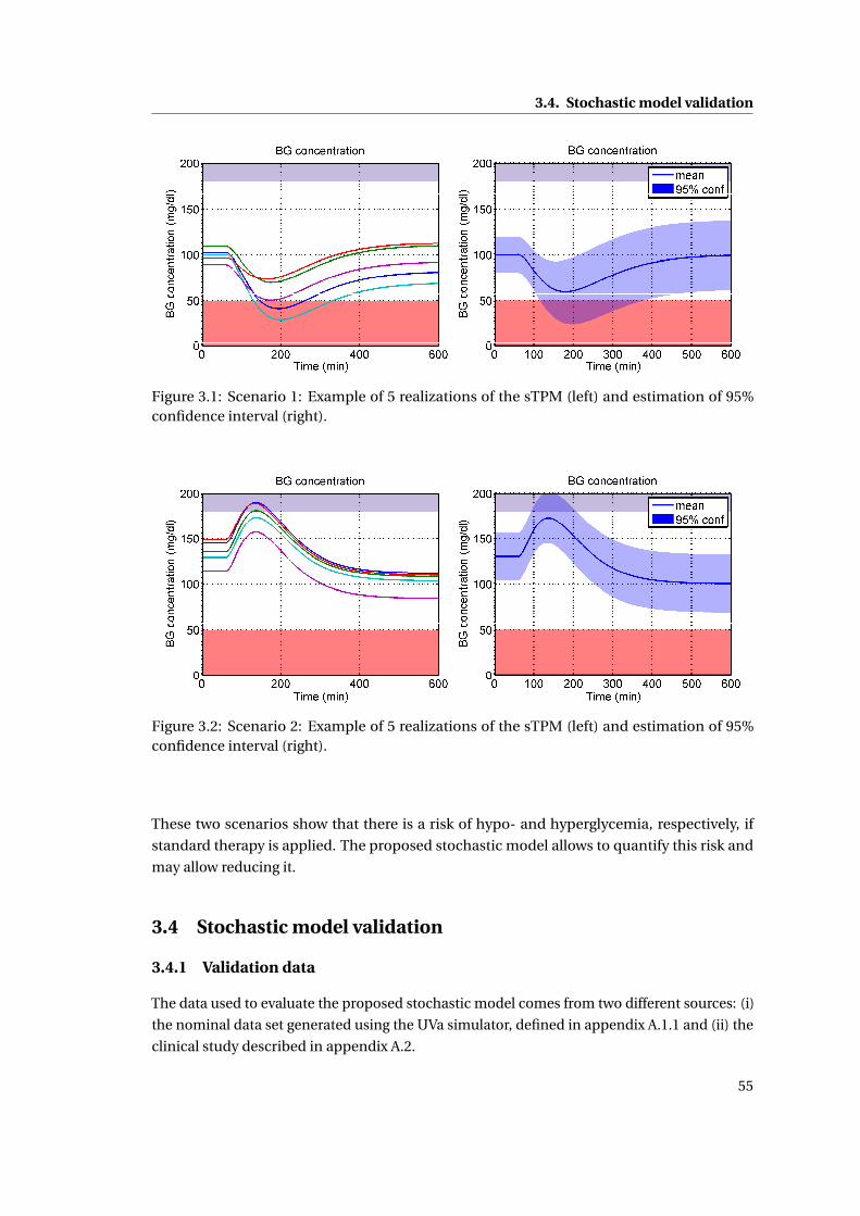
3.4. Stochastic model validation
Figure 3.1: Scenario 1: Example of 5 realizations of the sTPM (left) and estimation of 95%confidence interval (right).
Figure 3.2: Scenario 2: Example of 5 realizations of the sTPM (left) and estimation of 95%confidence interval (right).
These two scenarios show that there is a risk of hypo- and hyperglycemia, respectively, if
standard therapy is applied. The proposed stochastic model allows to quantify this risk and
may allow reducing it.
3.4 Stochastic model validation
3.4.1 Validation data
The data used to evaluate the proposed stochastic model comes from two different sources: (i)
the nominal data set generated using the UVa simulator, defined in appendix A.1.1 and (ii) the
clinical study described in appendix A.2.
55
Chapter 3. Stochastic Modeling
3.4.2 Validation methods
Cross-validation
One should never use data for validation that was previously used for parameter identification.
Since 4 days of UVa simulator data and 7 or 6 days for study data (for SMBG and CGM data,
respectively) are available, cross-validation is performed. This consists in identifying model
parameters on all but one day and using the additional day for validation. This procedure is
done such that every day is used for validation once. This way, a maximum of 4 validations for
every adult on the UVa simulator can be obtained, which leads to a total of 40 experiments.
For clinical study data, this would add up to 70 (respectively 60 for CGM data), however,
because, for some patients some days were disregarded, the number of separate validations
is 58 (respectively 52 for CGM data). These results are then averaged in order to evaluate
performance.
Choice of identification and validation data
For each of the two data sources, two different measurements are available: the exact BG and
CGM for the UVa simulator, and SMBG and CGM measurements for clinical study data. This
means that there are 8 possible validation cases (cf table 3.1) depending on what measure-
ments are used for identification and validation. For the sake of brevity, only a few cases are
case data origin identification data validation data
1 UVa simulator exact BG exact BG2 UVa simulator CGM exact BG3 UVa simulator exact CGM4 UVa simulator CGM CGM5 clinical study SMBG SMBG6 clinical study CGM SMBG7 clinical study SMBG CGM8 clinical study CGM CGM
Table 3.1: Possible validation cases
analyzed in detail. The main goal of the proposed method is to obtain probabilistic estimations
of the patient’s actual BG concentration. These estimations should be as exact as possible
when parameters are identified on measurements. For this reason, stochastic predictions
should always be compared with the most accurate measurement that is available. Therefore,
only cases 2,5, and 6 are analyzed in detail and the other cases are used to show particular
model properties.
The initialization of G and PBG is always done with respect to the measurements used for
identification. This means that if parameters are identified on CGM, exact, or SMBG data,
then G is initialized with CGM, exact, or SMBG measurements, respectively. PBG is initialized
according to equation 3.34 with r=20%, r= 0%, or r=10%, respectively.
56
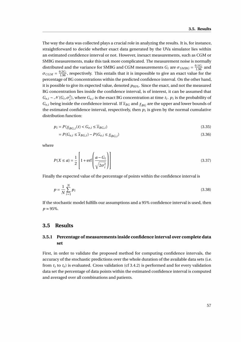
3.5. Results
The way the data was collected plays a crucial role in analyzing the results. It is, for instance,
straightforward to decide whether exact data generated by the UVa simulator lies within
an estimated confidence interval or not. However, inexact measurements, such as CGM or
SMBG measurements, make this task more complicated. The measurement noise is normally
distributed and the variance for SMBG and CGM measurements Gi are σSMBG = 0.1Gi1.96 and
σCGM = 0.2Gi1.96 , respectively. This entails that it is impossible to give an exact value for the
percentage of BG concentrations within the predicted confidence interval. On the other hand,
it is possible to give its expected value, denoted p95%. Since the exact, and not the measured
BG concentration lies inside the confidence interval, is of interest, it can be assumed that
Ge,i ∼N (Gi ,σ2i ), where Ge,i is the exact BG concentration at time ti . pi is the probability of
Ge,i being inside the confidence interval. If xBG and xBG are the upper and lower bounds of
the estimated confidence interval, respectively, then pi is given by the normal cumulative
distribution function:
pi = P (xBG ,i (t ) <Ge,i ≤ xBG ,i ) (3.35)
= P (Ge,i ≤ xBG ,i )−P (Ge,i ≤ xBG ,i ) (3.36)
where
P (X ≤ a) = 1
2
1+erf
a −Gi√2σ2
i
(3.37)
Finally the expected value of the percentage of points within the confidence interval is
p = 1
N
N∑i=1
pi (3.38)
If the stochastic model fulfills our assumptions and a 95% confidence interval is used, then
p ≈ 95%.
3.5 Results
3.5.1 Percentage of measurements inside confidence interval over complete dataset
First, in order to validate the proposed method for computing confidence intervals, the
accuracy of the stochastic predictions over the whole duration of the available data sets (i.e.
from ts to te ) is evaluated. Cross validation (cf 3.4.2) is performed and for every validation
data set the percentage of data points within the estimated confidence interval is computed
and averaged over all combinations and patients.
57
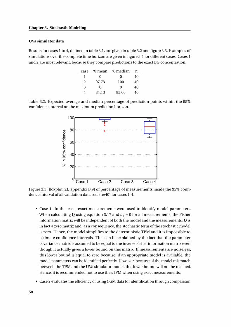
Chapter 3. Stochastic Modeling
UVa simulator data
Results for cases 1 to 4, defined in table 3.1, are given in table 3.2 and figure 3.3. Examples of
simulations over the complete time horizon are given in figure 3.4 for different cases. Cases 1
and 2 are most relevant, because they compare predictions to the exact BG concentration.
case % mean % median n1 0 0 402 97.73 100 403 0 0 404 84.13 85.00 40
Table 3.2: Expected average and median percentage of prediction points within the 95%confidence interval on the maximum prediction horizon.
0
20
40
60
80
100
Case 1 Case 2 Case 3 Case 4
% in
95%
con
fiden
ce
Figure 3.3: Boxplot (cf. appendix B.9) of percentage of measurements inside the 95% confi-dence interval of all validation data sets (n=40) for cases 1-4.
• Case 1: In this case, exact measurements were used to identify model parameters.
When calculating Q using equation 3.17 and σi = 0 for all measurements, the Fisher
information matrix will be independent of both the model and the measurements. Q is
in fact a zero matrix and, as a consequence, the stochastic term of the stochastic model
is zero. Hence, the model simplifies to the deterministic TPM and it is impossible to
estimate confidence intervals. This can be explained by the fact that the parameter
covariance matrix is assumed to be equal to the inverse Fisher information matrix even
though it actually gives a lower bound on this matrix. If measurements are noiseless,
this lower bound is equal to zero because, if an appropriate model is available, the
model parameters can be identified perfectly. However, because of the model mismatch
betweeb the TPM and the UVa simulator model, this lower bound will not be reached.
Hence, it is recommended not to use the sTPM when using exact measurements.
• Case 2 evaluates the efficiency of using CGM data for identification through comparison
58
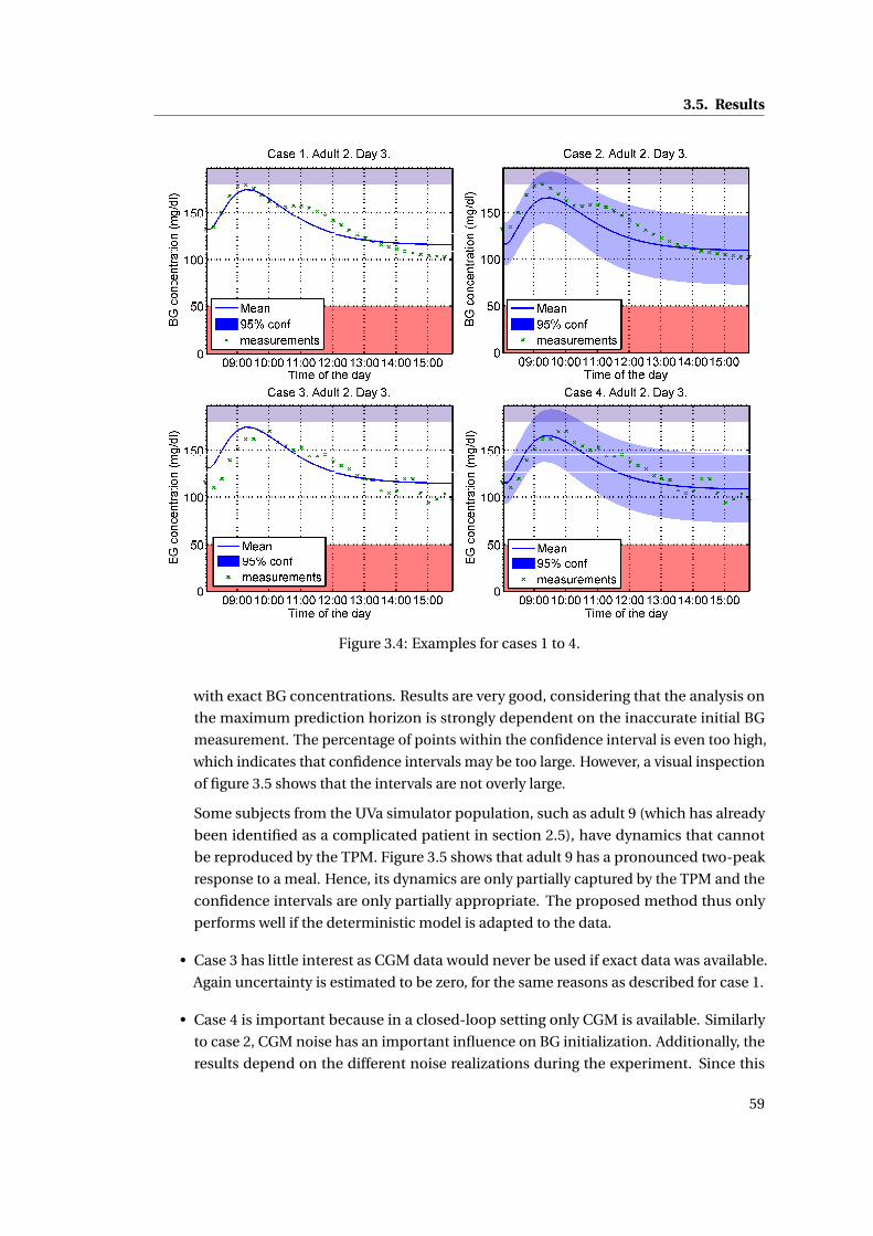
3.5. Results
Figure 3.4: Examples for cases 1 to 4.
with exact BG concentrations. Results are very good, considering that the analysis on
the maximum prediction horizon is strongly dependent on the inaccurate initial BG
measurement. The percentage of points within the confidence interval is even too high,
which indicates that confidence intervals may be too large. However, a visual inspection
of figure 3.5 shows that the intervals are not overly large.
Some subjects from the UVa simulator population, such as adult 9 (which has already
been identified as a complicated patient in section 2.5), have dynamics that cannot
be reproduced by the TPM. Figure 3.5 shows that adult 9 has a pronounced two-peak
response to a meal. Hence, its dynamics are only partially captured by the TPM and the
confidence intervals are only partially appropriate. The proposed method thus only
performs well if the deterministic model is adapted to the data.
• Case 3 has little interest as CGM data would never be used if exact data was available.
Again uncertainty is estimated to be zero, for the same reasons as described for case 1.
• Case 4 is important because in a closed-loop setting only CGM is available. Similarly
to case 2, CGM noise has an important influence on BG initialization. Additionally, the
results depend on the different noise realizations during the experiment. Since this
59
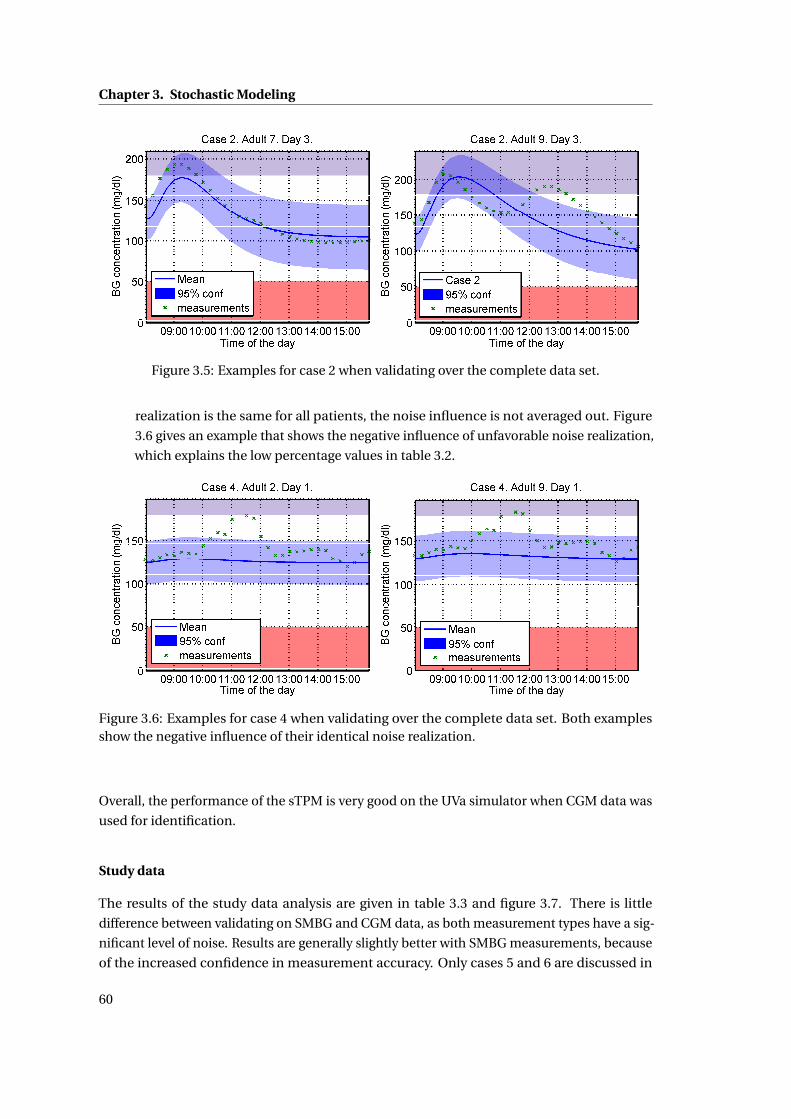
Chapter 3. Stochastic Modeling
Figure 3.5: Examples for case 2 when validating over the complete data set.
realization is the same for all patients, the noise influence is not averaged out. Figure
3.6 gives an example that shows the negative influence of unfavorable noise realization,
which explains the low percentage values in table 3.2.
Figure 3.6: Examples for case 4 when validating over the complete data set. Both examplesshow the negative influence of their identical noise realization.
Overall, the performance of the sTPM is very good on the UVa simulator when CGM data was
used for identification.
Study data
The results of the study data analysis are given in table 3.3 and figure 3.7. There is little
difference between validating on SMBG and CGM data, as both measurement types have a sig-
nificant level of noise. Results are generally slightly better with SMBG measurements, because
of the increased confidence in measurement accuracy. Only cases 5 and 6 are discussed in
60
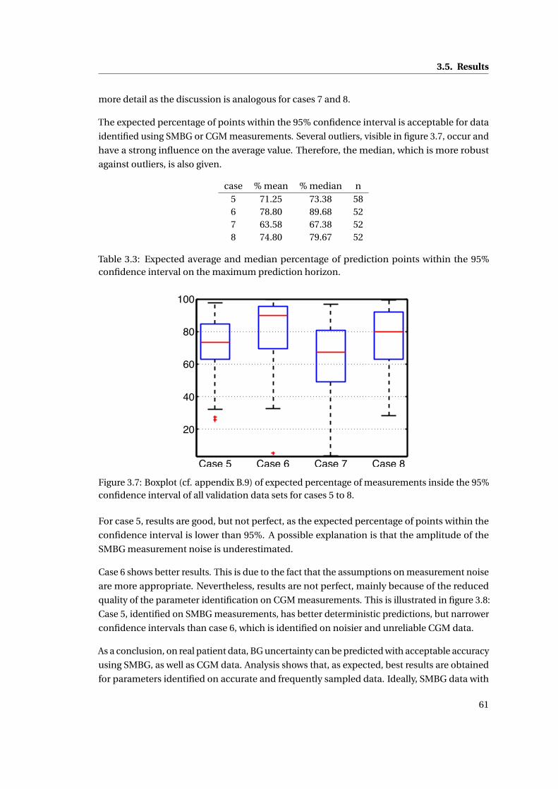
3.5. Results
more detail as the discussion is analogous for cases 7 and 8.
The expected percentage of points within the 95% confidence interval is acceptable for data
identified using SMBG or CGM measurements. Several outliers, visible in figure 3.7, occur and
have a strong influence on the average value. Therefore, the median, which is more robust
against outliers, is also given.
case % mean % median n5 71.25 73.38 586 78.80 89.68 527 63.58 67.38 528 74.80 79.67 52
Table 3.3: Expected average and median percentage of prediction points within the 95%confidence interval on the maximum prediction horizon.
20
40
60
80
100
Case 5 Case 6 Case 7 Case 8Figure 3.7: Boxplot (cf. appendix B.9) of expected percentage of measurements inside the 95%confidence interval of all validation data sets for cases 5 to 8.
For case 5, results are good, but not perfect, as the expected percentage of points within the
confidence interval is lower than 95%. A possible explanation is that the amplitude of the
SMBG measurement noise is underestimated.
Case 6 shows better results. This is due to the fact that the assumptions on measurement noise
are more appropriate. Nevertheless, results are not perfect, mainly because of the reduced
quality of the parameter identification on CGM measurements. This is illustrated in figure 3.8:
Case 5, identified on SMBG measurements, has better deterministic predictions, but narrower
confidence intervals than case 6, which is identified on noisier and unreliable CGM data.
As a conclusion, on real patient data, BG uncertainty can be predicted with acceptable accuracy
using SMBG, as well as CGM data. Analysis shows that, as expected, best results are obtained
for parameters identified on accurate and frequently sampled data. Ideally, SMBG data with
61
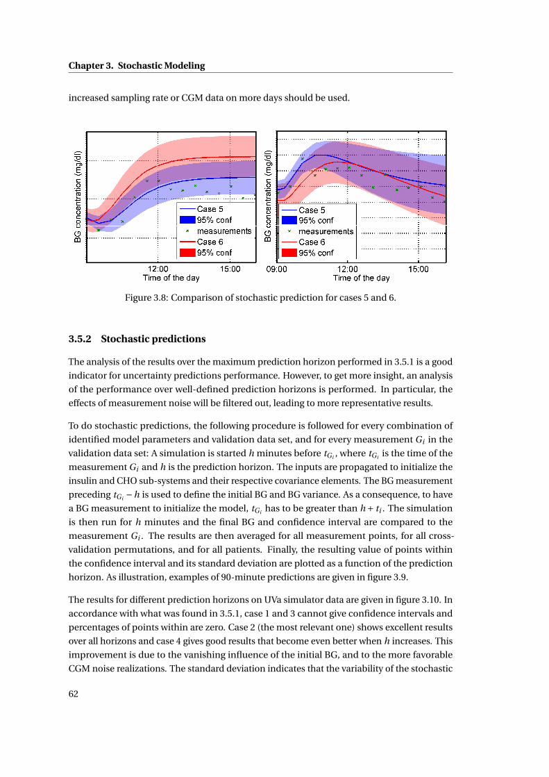
Chapter 3. Stochastic Modeling
increased sampling rate or CGM data on more days should be used.
Figure 3.8: Comparison of stochastic prediction for cases 5 and 6.
3.5.2 Stochastic predictions
The analysis of the results over the maximum prediction horizon performed in 3.5.1 is a good
indicator for uncertainty predictions performance. However, to get more insight, an analysis
of the performance over well-defined prediction horizons is performed. In particular, the
effects of measurement noise will be filtered out, leading to more representative results.
To do stochastic predictions, the following procedure is followed for every combination of
identified model parameters and validation data set, and for every measurement Gi in the
validation data set: A simulation is started h minutes before tGi , where tGi is the time of the
measurement Gi and h is the prediction horizon. The inputs are propagated to initialize the
insulin and CHO sub-systems and their respective covariance elements. The BG measurement
preceding tGi −h is used to define the initial BG and BG variance. As a consequence, to have
a BG measurement to initialize the model, tGi has to be greater than h + ti . The simulation
is then run for h minutes and the final BG and confidence interval are compared to the
measurement Gi . The results are then averaged for all measurement points, for all cross-
validation permutations, and for all patients. Finally, the resulting value of points within
the confidence interval and its standard deviation are plotted as a function of the prediction
horizon. As illustration, examples of 90-minute predictions are given in figure 3.9.
The results for different prediction horizons on UVa simulator data are given in figure 3.10. In
accordance with what was found in 3.5.1, case 1 and 3 cannot give confidence intervals and
percentages of points within are zero. Case 2 (the most relevant one) shows excellent results
over all horizons and case 4 gives good results that become even better when h increases. This
improvement is due to the vanishing influence of the initial BG, and to the more favorable
CGM noise realizations. The standard deviation indicates that the variability of the stochastic
62
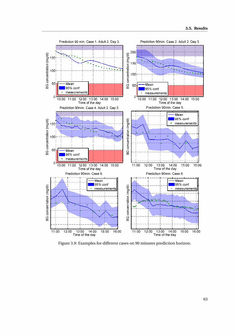
3.5. Results
Figure 3.9: Examples for different cases on 90 minutes prediction horizon.
63
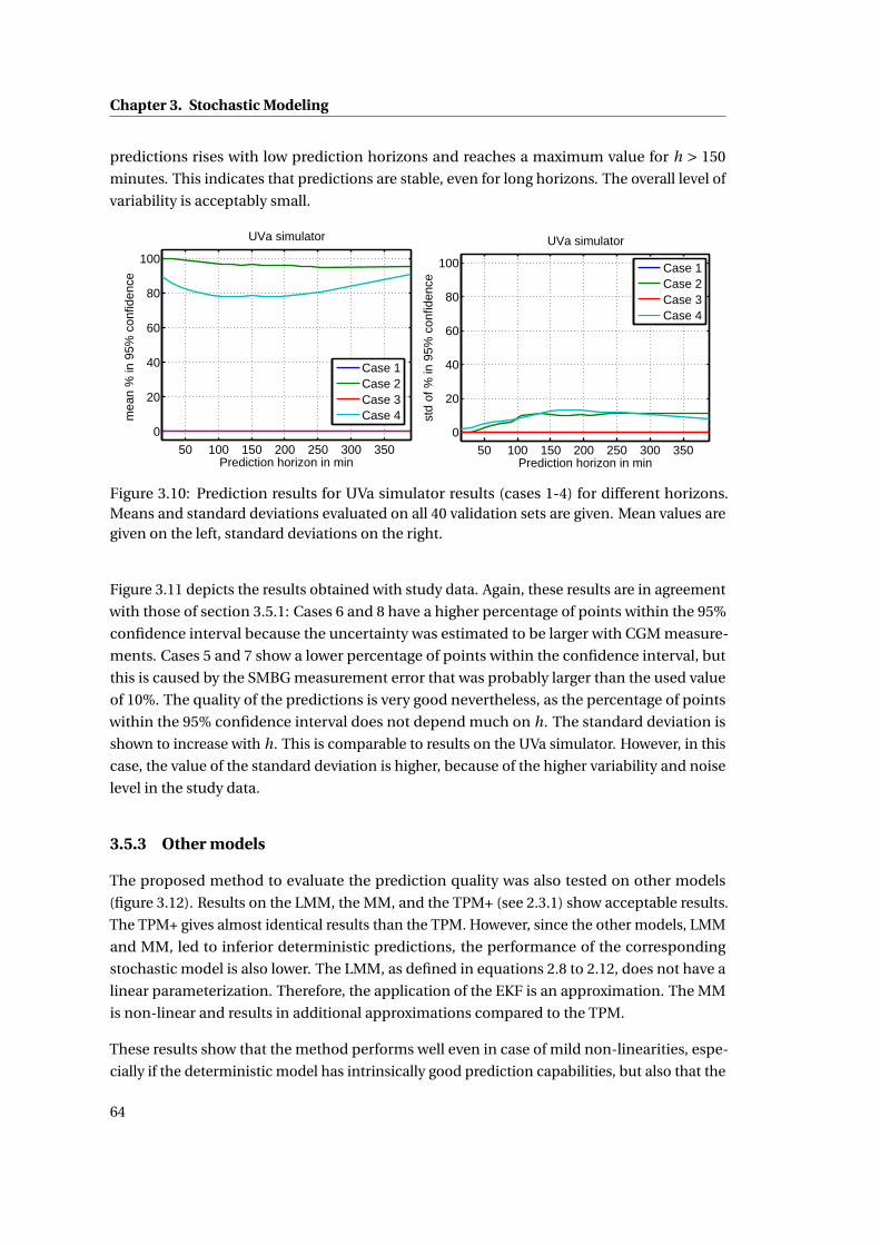
Chapter 3. Stochastic Modeling
predictions rises with low prediction horizons and reaches a maximum value for h > 150
minutes. This indicates that predictions are stable, even for long horizons. The overall level of
variability is acceptably small.
50 100 150 200 250 300 350
0
20
40
60
80
100
Prediction horizon in min
mea
n %
in 9
5% c
onfid
ence
UVa simulator
Case 1Case 2Case 3Case 4
50 100 150 200 250 300 350
0
20
40
60
80
100
Prediction horizon in min
std
of %
in 9
5% c
onfid
ence
UVa simulator
Case 1Case 2Case 3Case 4
Figure 3.10: Prediction results for UVa simulator results (cases 1-4) for different horizons.Means and standard deviations evaluated on all 40 validation sets are given. Mean values aregiven on the left, standard deviations on the right.
Figure 3.11 depicts the results obtained with study data. Again, these results are in agreement
with those of section 3.5.1: Cases 6 and 8 have a higher percentage of points within the 95%
confidence interval because the uncertainty was estimated to be larger with CGM measure-
ments. Cases 5 and 7 show a lower percentage of points within the confidence interval, but
this is caused by the SMBG measurement error that was probably larger than the used value
of 10%. The quality of the predictions is very good nevertheless, as the percentage of points
within the 95% confidence interval does not depend much on h. The standard deviation is
shown to increase with h. This is comparable to results on the UVa simulator. However, in this
case, the value of the standard deviation is higher, because of the higher variability and noise
level in the study data.
3.5.3 Other models
The proposed method to evaluate the prediction quality was also tested on other models
(figure 3.12). Results on the LMM, the MM, and the TPM+ (see 2.3.1) show acceptable results.
The TPM+ gives almost identical results than the TPM. However, since the other models, LMM
and MM, led to inferior deterministic predictions, the performance of the corresponding
stochastic model is also lower. The LMM, as defined in equations 2.8 to 2.12, does not have a
linear parameterization. Therefore, the application of the EKF is an approximation. The MM
is non-linear and results in additional approximations compared to the TPM.
These results show that the method performs well even in case of mild non-linearities, espe-
cially if the deterministic model has intrinsically good prediction capabilities, but also that the
64
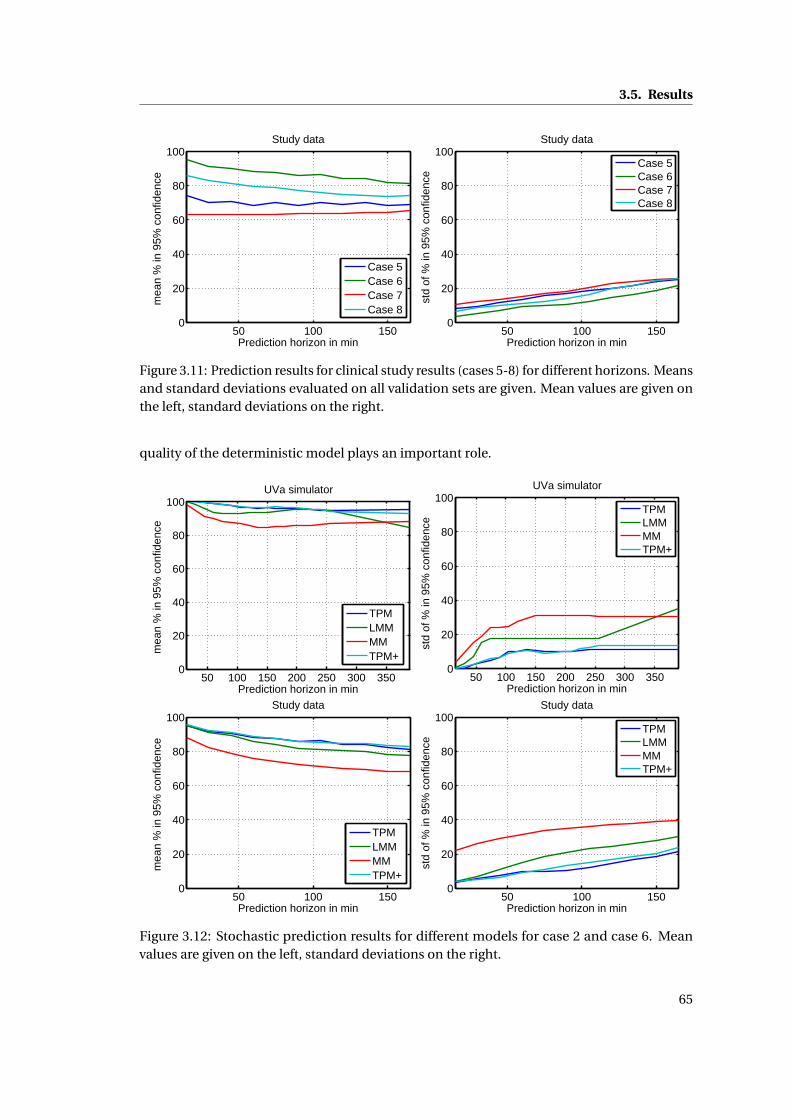
3.5. Results
50 100 1500
20
40
60
80
100
Prediction horizon in min
mea
n %
in 9
5% c
onfid
ence
Study data
Case 5Case 6Case 7Case 8
50 100 1500
20
40
60
80
100
Prediction horizon in min
std
of %
in 9
5% c
onfid
ence
Study data
Case 5Case 6Case 7Case 8
Figure 3.11: Prediction results for clinical study results (cases 5-8) for different horizons. Meansand standard deviations evaluated on all validation sets are given. Mean values are given onthe left, standard deviations on the right.
quality of the deterministic model plays an important role.
50 100 150 200 250 300 3500
20
40
60
80
100
Prediction horizon in min
mea
n %
in 9
5% c
onfid
ence
UVa simulator
TPMLMMMMTPM+
50 100 150 200 250 300 3500
20
40
60
80
100
Prediction horizon in min
std
of %
in 9
5% c
onfid
ence
UVa simulator
TPMLMMMMTPM+
50 100 1500
20
40
60
80
100
Prediction horizon in min
mea
n %
in 9
5% c
onfid
ence
Study data
TPMLMMMMTPM+
50 100 1500
20
40
60
80
100
Prediction horizon in min
std
of %
in 9
5% c
onfid
ence
Study data
TPMLMMMMTPM+
Figure 3.12: Stochastic prediction results for different models for case 2 and case 6. Meanvalues are given on the left, standard deviations on the right.
65
Chapter 3. Stochastic Modeling
3.6 Conclusion
A novel method, to construct a stochastic model based on parametric uncertainty and to
propagate these uncertainties, was presented and applied to the TPM. This new approach
allows computing confidence intervals on BG concentrations in a simple, yet effective way.
It performs as expected, although the designed stochastic models are always just as good as
their underlying deterministic models. As such, it is important that the latter be adapted to
the modeled system. Validation was performed on UVa simulator data, as well as clinical
data and results for both were good for the relevant cases. Since clinical data contains more
unpredictable events, estimation results were slightly worse than with UVa simulator data.
The estimation of BG uncertainty is an invaluable addition to improve diabetes treatment.
The use of the stochastic information allows reducing patient’s hypo- and hyperglycemia
risk, especially in combination with a CGM device. However, the expected percentage of
points within the 95% confidence interval is not 95% as it should be, if all assumptions were
satisfied. Hence, more than 5% of the points lie outside the estimated confidence interval.
This has numerous causes, such as non-Gaussian noise, different sources of non-linearities,
or exceptional intra-patient variability. Nevertheless, using the stochastic information is
beneficial in all circumstances: if the uncertainty is reliably estimated, patients can be treated
while considerably reducing hypo- and hyperglycemia risk. Furthermore, if the uncertainty is
estimated to be larger than it actually is, patients still have a lowered risk for large glycemic
deviations, but may need to take more SMBG measurements to reduce the conservatism of
the resulting recommendations of insulin injections. If uncertainties are underestimated, on
the one hand, treatment is still safer than without uncertainty estimations and, on the other
hand, if a CGM device is used, inaccuracies can immediately be detected and parameters can
be adapted accordingly.
The newly designed sTPM will be used for new applications in the two following chapters.
It should be noted that the application field of this new method is not limited to diabetes
management, but may be applied to any process in which a large uncertainty is present and
needs to be estimated. Also, the application is not limited to parametric uncertainty, but can
be extended to take input uncertainty into account. For example the uncertainty in meal
amounts, discussed in section 1.2.2, could be addressed.
66
4 BG estimation
4.1 Introduction
One of the objectives of this thesis is to improve the treatment of diabetes using control
methods. However, in order to do control - may it be standard therapy, open-loop, or closed-
loop control - good quality BG, or full state estimation (i.e. estimating all states and not only
BG) are essential. The most straightforward way to obtain BG estimations is to use one of the
measurement devices described in 1.1.2: SMBG is commonly used for standard therapy or
open-loop control, while CGM is required for an AP, but is also useful for open-loop control.
However, with these devices, measurement noise contributes to the uncertainty that makes BG
control a challenge, as described in 1.2.2. The measurement noise is detrimental to treatment
and its impact should be minimized. Since SMBG measurements are taken irregularly with
potentially low sampling frequency, it is almost impossible to improve these measurements
significantly. CGM measurements, on the other hand, have a sampling time of about one
minute, but have a rather large noise level. This sampling time is much smaller than what
would be required for treatment, as an AP is usually sampled every 5 minutes, even though 20
minutes would be sufficient (cf. 5.3.3). Therefore, the redundant measurements can be used
to filter out high measurement noise and improve the BG estimates at the relevant instants.
For some closed-loop controllers, it is also necessary to have access to the full system state, in
which case, a complete state estimation using CGM measurements can be done.
In the literature, CGM data is almost always filtered or used for state estimation, and the
most commonly used technique is by far the Kalman filter (KF). There are many different
implementations such as, for example, a KF with adaptive signal-to-noise ratio by Facchinetti
et al. [2011]. Knobbe and Buckingham [2005] propose an EKF, i.e. a non-linear KF, and Kuure-
Kinsey et al. [2006] discuss a dual-rate KF that takes into account both CGM measurements
and SMBG calibration measurements. While most of these filters work relatively well, their
performance still depends on the underlying model. However, as discussed and shown in
chapter 2, the models, typically used for control or prediction, are not very well adapted to
these tasks and may lead to unacceptable results. Another drawback is that these models do
67
Chapter 4. BG estimation
not account for other available information like insulin infusions or meal intakes.
In this chapter, in order to improve the available BG concentration information, several well-
known estimation techniques of varying complexity are adapted for diabetes treatment. The
individualized TPM, TPM+, or sTPM that allow better model predictions and take inputs such
as meal announcements or insulin infusions into account are at the heart of these techniques.
The BG concentrations estimated using the proposed filters are shown to be superior for
diabetes treatment (evaluated using the Clarke EGA described in B.3) as demonstrated on the
UVa simulator.
This chapter is organized as follows: First, in section 4.2, the observability of the TPM and the
TPM+ is verified as this is a necessary condition for the application of moste state estimation
algorithms. Section 4.3 describes the different estimators that will then be compared on UVa
simulator data in section 4.5, using the methods described in section 4.4. Final considerations
are made and a conclusion is drawn in section 4.6.
4.2 Observability
The proposed model-based estimation techniques require the deterministic part of the model
to be observable - a property that is further defined below. A first step for checking model
observability is to put it into the standard linear state-space form.
4.2.1 State-space representation
The state-space representation was already introduced in equation 3.1 in its general form.
However, since the TPM and the TPM+ are linear, the linear state-space representation, which
is fully specified by the definition of 3 matrices, can be used.
The linear state-space equations are defined as follows where the output is considered to be
linear with respect to the states:
x(t ) = Ax(t )+Bu(t ) (4.1)
y(t ) = Cx(t ), (4.2)
where A is the n-by-n state matrix, with n being the number of states, x is the n-by-1 state
vector, B is the n-by-m input matrix, with m being the number of inputs, u is the m-by-1 input
vector, y is the p-by-1 output vector, with p being the number of outputs, and C is the p-by-n
output matrix.
The two new control-specific models, designed in chapter 2, are given in this representa-
tion below. Since only BG concentration is assumed to be measured, the output is the BG
concentration state G .
68
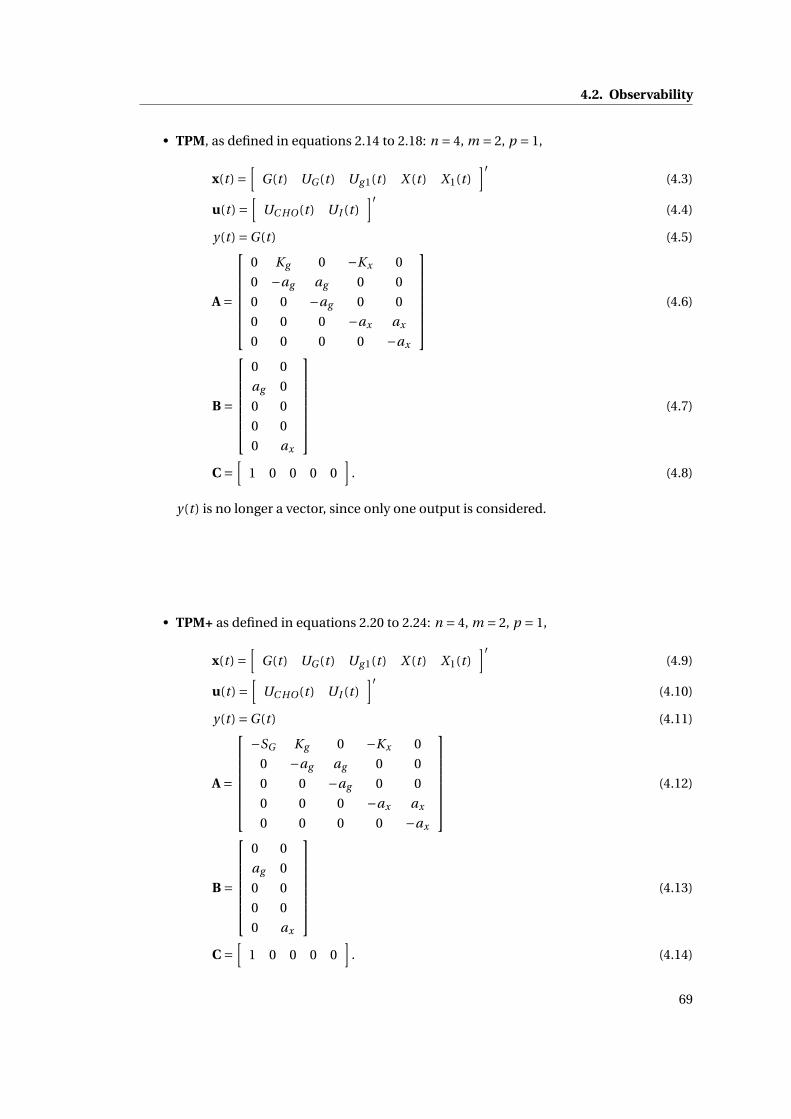
4.2. Observability
• TPM, as defined in equations 2.14 to 2.18: n = 4, m = 2, p = 1,
x(t ) =[
G(t ) UG (t ) Ug 1(t ) X (t ) X1(t )]′
(4.3)
u(t ) =[
UC HO(t ) UI (t )]′
(4.4)
y(t ) =G(t ) (4.5)
A =
0 Kg 0 −Kx 0
0 −ag ag 0 0
0 0 −ag 0 0
0 0 0 −ax ax
0 0 0 0 −ax
(4.6)
B =
0 0
ag 0
0 0
0 0
0 ax
(4.7)
C =[
1 0 0 0 0]
. (4.8)
y(t ) is no longer a vector, since only one output is considered.
• TPM+ as defined in equations 2.20 to 2.24: n = 4, m = 2, p = 1,
x(t ) =[
G(t ) UG (t ) Ug 1(t ) X (t ) X1(t )]′
(4.9)
u(t ) =[
UC HO(t ) UI (t )]′
(4.10)
y(t ) =G(t ) (4.11)
A =
−SG Kg 0 −Kx 0
0 −ag ag 0 0
0 0 −ag 0 0
0 0 0 −ax ax
0 0 0 0 −ax
(4.12)
B =
0 0
ag 0
0 0
0 0
0 ax
(4.13)
C =[
1 0 0 0 0]
. (4.14)
69
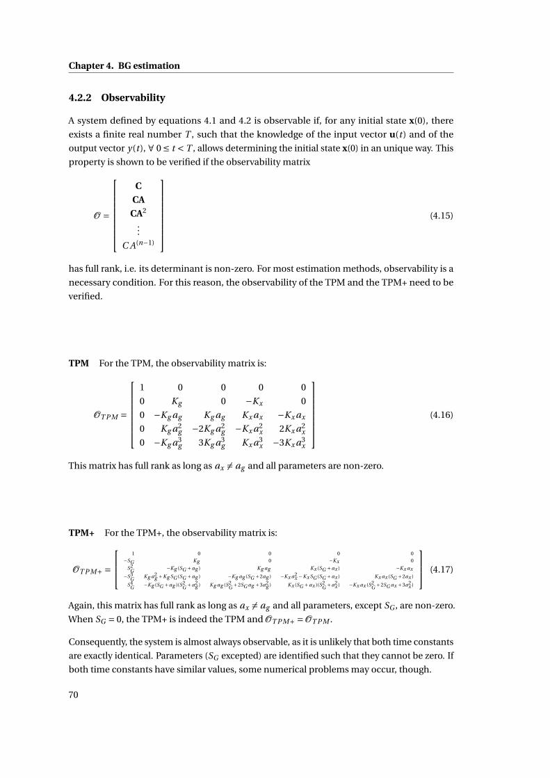
Chapter 4. BG estimation
4.2.2 Observability
A system defined by equations 4.1 and 4.2 is observable if, for any initial state x(0), there
exists a finite real number T , such that the knowledge of the input vector u(t) and of the
output vector y(t ), ∀ 0 ≤ t < T , allows determining the initial state x(0) in an unique way. This
property is shown to be verified if the observability matrix
O =
C
CA
CA2
...
C A(n−1)
(4.15)
has full rank, i.e. its determinant is non-zero. For most estimation methods, observability is a
necessary condition. For this reason, the observability of the TPM and the TPM+ need to be
verified.
TPM For the TPM, the observability matrix is:
OT P M =
1 0 0 0 0
0 Kg 0 −Kx 0
0 −Kg ag Kg ag Kx ax −Kx ax
0 Kg a2g −2Kg a2
g −Kx a2x 2Kx a2
x
0 −Kg a3g 3Kg a3
g Kx a3x −3Kx a3
x
(4.16)
This matrix has full rank as long as ax 6= ag and all parameters are non-zero.
TPM+ For the TPM+, the observability matrix is:
OT P M+ =
1 0 0 0 0
−SG Kg 0 −Kx 0
S2G −Kg (SG +ag ) Kg ag Kx (SG +ax ) −Kx ax
−S3G Kg a2
g +Kg SG (SG +ag ) −Kg ag (SG +2ag ) −Kx a2x −Kx SG (SG +ax ) Kx ax (SG +2ax )
S4G −Kg (SG +ag )(S2
G +a2g ) Kg ag (S2
G +2SG ag +3a2g ) Kx (SG +ax )(S2
G +a2x ) −Kx ax (S2
G +2SG ax +3a2x )
(4.17)
Again, this matrix has full rank as long as ax 6= ag and all parameters, except SG , are non-zero.
When SG = 0, the TPM+ is indeed the TPM and OT P M+ =OT P M .
Consequently, the system is almost always observable, as it is unlikely that both time constants
are exactly identical. Parameters (SG excepted) are identified such that they cannot be zero. If
both time constants have similar values, some numerical problems may occur, though.
70
4.3. Different BG estimators
4.3 Different BG estimators
Now that the conditions for observability have been verified, the different BG estimators that
will be compared on the UVa simulator in this chapter, can be introduced in the following
paragraphs, ordered by increasing complexity. Since these estimators are evaluated on UVa
simulator data, the TPM is used as a prediction model, but can be replaced by the TPM+ if real
patient data is to be used.
4.3.1 Low-pass filter
The most obvious and simple way to filter a noisy signal with high sample frequency is to use a
traditional low-pass filter, such as a Butterworth filter. This kind of filter damps all information
with a frequency higher than the so-called cutoff frequency. This results in a smoother signal,
but a delay will appear. The cutoff frequency ωc , which is the tuning parameter, should be
slightly higher than the frequency corresponding to the system’s smallest time constant. A
first-order filter is typically chosen to reduce filter latency. The problem with this approach is
that such a filter introduces a new delay that is relatively long if the cutoff frequency is low.
For this reason a model-based method is probably better suited for this purpose. Also, the
low-pass filter is sensitive to sensor dropouts because no model information is used. The
transfer function of the low-pass filter is:
H(s) = 11ωc
s +1. (4.18)
The time constant of the filter was chosen to be 10% faster than the fastest system time
constant (which is around 20 minutes on UVa simulator data).
4.3.2 Luenberger observer
A classical state-space observer such as the Luenberger observer is a common candidate for
determining unmeasured states or filtering measurements, and is used by Svensson [2013],
e.g.. The estimation achieved using the following continuous-time equations
˙x(t ) = Ax(t )+Bu(t )+L(y(t )−Cx(t )), (4.19)
where x is the estimated state and L is the n-by-p observer gain matrix. In other words, a
Luenberger observer is based on open-loop observer that is corrected using the weighted
estimation error. A schematic representation of this observer is given in figure 4.1.
The performance of this estimator depends, on the one hand, on the model that is being
used (in this case the new prediction models), and, on the other hand, on the tuning of the L
matrix. In the context of this thesis, as only BG concentration is measured, p equals 1 and,
therefore, L is a vector of dimension 5. This means that the system to be observed has multiple
71
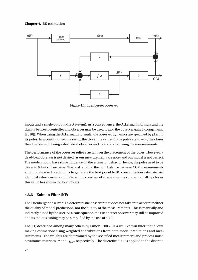
Chapter 4. BG estimation
-
Figure 4.1: Luenberger observer
inputs and a single output (MISO system). As a consequence, the Ackermann formula and the
duality between controller and observer may be used to find the observer gain L (Longchamp
[2010]). When using the Ackermann formula, the observer dynamics are specified by placing
its poles. In a continuous-time setup, the closer the values of the poles are to −∞, the closer
the observer is to being a dead-beat observer and to exactly following the measurements.
The performance of the observer relies crucially on the placement of the poles. However, a
dead-beat observer is not desired, as our measurements are noisy and our model is not perfect.
The model should have some influence on the estimator behavior, hence, the poles need to be
closer to 0, but still negative. The goal is to find the right balance between CGM measurements
and model-based predictions to generate the best possible BG concentration estimate. An
identical value, corresponding to a time constant of 40 minutes, was chosen for all 5 poles as
this value has shown the best results.
4.3.3 Kalman Filter (KF)
The Luenberger observer is a deterministic observer that does not take into account neither
the quality of model predictions, nor the quality of the measurements. This is manually and
indirectly tuned by the user. As a consequence, the Luenberger observer may still be improved
and its tedious tuning may be simplified by the use of a KF.
The KF, described among many others by Simon [2006], is a well-known filter that allows
making estimations using weighted contributions from both model predictions and mea-
surements. The weights are determined by the specified measurement and process noise
covariance matrices, R and QK F , respectively. The discretized KF is applied to the discrete
72
4.3. Different BG estimators
system defined by:
xk =Φxk−1 +Γuk−1 +wk−1 (4.20)
yk = Cxk +vk (4.21)
E(wk w′j ) = QK Fδk− j (4.22)
E(vk v′j ) = Rδk− j (4.23)
E(wk v′j ) = 0, (4.24)
whereΦ and Γ are the discretized matrices corresponding to A and B, respectively. xk , uk , wk ,
and yk are x(t ), u(t ), w(t ), and y(t ) at the k th sampling time. v(k) is the measurement noise at
the k th sampling time. wk and vk are Gaussian random variables whose covariance matrices
are defined by equations 4.22 to 4.24 and are thus uncorrelated. δk− j is the Kronecker delta
that equals 1 if k = j and 0 otherwise.
The discrete-time KF is given by equations 4.25 to 4.21, for each sampling time k.
P−k =ΦP+
k−1Φ′+QK F (4.25)
Kk = P−k C(P−
k C′+R)−1 (4.26)
x−k =Φx+k−1 +Γuk−1 (4.27)
x+k = x−k +Kk (yk −Cx−k ) (4.28)
P+k = (I−Kk C)P−
k (4.29)
yk = Cx+k , (4.30)
where Pk is P(t) at t = tk , and K is the Kalman filter gain. Since, during one KF iteration, Pk
and xk are updated, the superscripts − and + denote the values before and after the variable
update, respectively.
In this work, the discrete-time KF equations are applied to the TPM in discretized state-space
formulation. The discretization at a 1-minute sampling time, corresponding to the UVa
simulator, is evaluated numerically. Initial values are chosen as follows:
x+0 =[
G0 0 0 0 0]′
(4.31)
P+0 =
σ2
G ,0 0 0 0 0
0 0 0 0 0
0 0 0 0 0
0 0 0 0 0
0 0 0 0 0
, (4.32)
where, G0 is the initial measurement of BG, and σ2G ,0 is the variance attributed to G0.
73
Chapter 4. BG estimation
The two tuning parameters QK F and R are chosen as follows:
QK F =
QBG 0 0 0 0
0 0 0 0 0
0 0 0 0 0
0 0 0 0 0
0 0 0 0 0
(4.33)
QBG = cf. table 4.1 (4.34)
R = 100. (4.35)
The value of QBG is determined using the Root Mean Square Error (RMSE) of 1-minute ahead
predictions on UVa data, which reflects how well the TPM allows doing short predictions for
each patient. A generic value of 0.04 (mg/dl)2 also gives good results whenever a personaliza-
tion is not possible. The value of R is found by assuming that 95% of measurements are within
20% and that the average BG concentration is approximately 100 mg/dl:
R =(
0.2
1.96100
)2
≈ 102. (4.36)
It should be noted that a KF assumes a white Gaussian noise for both process and measurement
noise. However, this is only an assumption, as both of these noises are known to be correlated.
For example, the CGM noise in the UVa simulator is generated using the model developed by
Breton and Kovatchev [2008] that uses colored noise.
Adult 1 2 3 4 5 6 7 8 9 10√QBG 0.297 0.234 0.205 0.159 0.147 0.186 0.299 0.227 0.228 0.195
Table 4.1: Square root of QBG for all 10 patients in mg/dl.
4.3.4 Extended Kalman Filter with the sTPM (EKF)
The sTPM explicitly models process noise as a function of time. Specifically, after a bolus or a
meal, the confidence in the model decreases, as the outcome becomes less predictable. This
information may directly be used in a KF. However, the sTPM, as described in chapter 3, is not
linear because of the time and state dependence of the stochastic term. For this reason, an
EKF has to be used. As already mentioned, the sTPM being linearly parameterized, this is not
an approximation.
The sTPM can be expressed as:
xk =Φxk−1 +Γuk−1 +Lk−1wk−1 (4.37)
yk = Cxk + vk , (4.38)
74
4.3. Different BG estimators
where Lk is the discrete version of L(t) defined in equation 3.33 that depends on xk and uk .
The process noise is now defined by E(wk w′j ) = Qδk− j .
Because the EKF can account for non-linearities, the measurement noise variance can be
expressed as a function of BG concentration, based on the ISO 15197 norm that imposes a
20% error:
Rk =(
0.2
1.96Gk
)2
, (4.39)
where Gk is the BG concentration at the k th sample. As a consequence, high BG measurements
have higher uncertainty than lower ones.
The EKF is given by the following equations:
P−k =ΦP+
k−1Φ′+Lk−1QL′
k−1 (4.40)
Kk = P−k C(P−
k C′+ yk Rk yk )−1 (4.41)
x−k =Φx+k−1 +Γuk−1 (4.42)
x+k = x−k +Kk (yk −Cx−k ) (4.43)
P+k = (I−Kk C)P−
k (4.44)
yk = Cx+k . (4.45)
Q is determined using the inverse Fisher information matrix as described in section 3.4. Initial
values for x and P are the same as for the KF.
4.3.5 Extended Kalman Filter with sTPM and added process noise - the TherapyParameter-based Filter (TPF)
As the noise level in the EKF can be shown to be insufficient (section 4.5), the process noise
used for the KF and for the EKF can be combined to have a more realistic noise term. In this
case, the noise term Lk−1wk−1 is augmented by increasing the dimension of Lk and Q by one.
This can easily be done by adding a term to equation 4.40. This new EKF will be referred to as
Therapy Parameter-based Filter (TPF). Its equations can be written as:
P−k =ΦP+
k−1Φ′+Lk−1QL′
k−1 +QK F (4.46)
Kk = P−k C(P−
k C′+ yk Rk yk )−1 (4.47)
x−k =Φx+k−1 +Γuk−1 (4.48)
x+k = x−k +Kk (yk −Cx−k ) (4.49)
P+k = (I−Kk C)P−
k (4.50)
yk = Cx+k , (4.51)
75
Chapter 4. BG estimation
where QK F is given in equation 4.33. Initial values for x and P are the same as for the KF.
4.4 Methods to compare CGM filters
As was already explained in section 2.5 and 3.4, the data used to determine model parameters
should never be used to validate results. For this reason, separate sets of training data and
validation data are generated using the UVa simulator. The methods are not tested on real
patient data because no accurate reference measurements are available. As such, this analysis
is limited to the UVa simulator and results are only valid within this scope. Therefore, the
TPM and the sTPM are used, rather than the TPM+ that would be recommended on real
patient data. To compare the results for different filters, several metrics are necessary that are
discussed in this section.
4.4.1 Training data
The proposed filters (except the Butterworth filter) are based on models, whose parameters
need to be identified for every subject out of the 10-patient database of the UVa simulator. For
this reason, the model parameters are identified on different sensitivity test days, which are
specified in more detail in appendix A.1.2. These test days consist in 3 insulin sensitivity and 3
meal sensitivity tests, performed to obtain reliable insulin action (cf. 2.4.3).
As explained in 2.5.1, neither the TPM, nor the TPM+ is able to fit sensitivity test data, because
their dynamics are not fully compatible with the UVa simulator model. Nevertheless, it is
possible to fit these models on sensitivity test data when the BG measurements taken after
the maximum or minimum of the meal or insulin sensitivity test, respectively, are discarded.
This procedure leads to accurate model parameters that have very reliable insulin action. To
identify the parameters, an analogous procedure to that of section 2.4.2 was used.
Simulated CGM measurements are used for parameter identification. This makes the identifi-
cation of the parameter covariance matrix possible, with the approach of section 3.2.3.
4.4.2 Validation data
To validate and compare the proposed filtering algorithms, 4 consecutive days of UVa simulator
data are available. These are described in more detail in appendix A.1.1 and consist in 3
standard therapy days and one day with "random" insulin infusions and meal intakes. The
simulated CGM results are filtered and compared to the exact BG values.
The validation relies on 3 scenarios, each leading to slightly different results and showing
advantages and drawbacks of the different formulations:
• Scenario 1: Data from the third standard therapy day illustrates how the filters compare
76
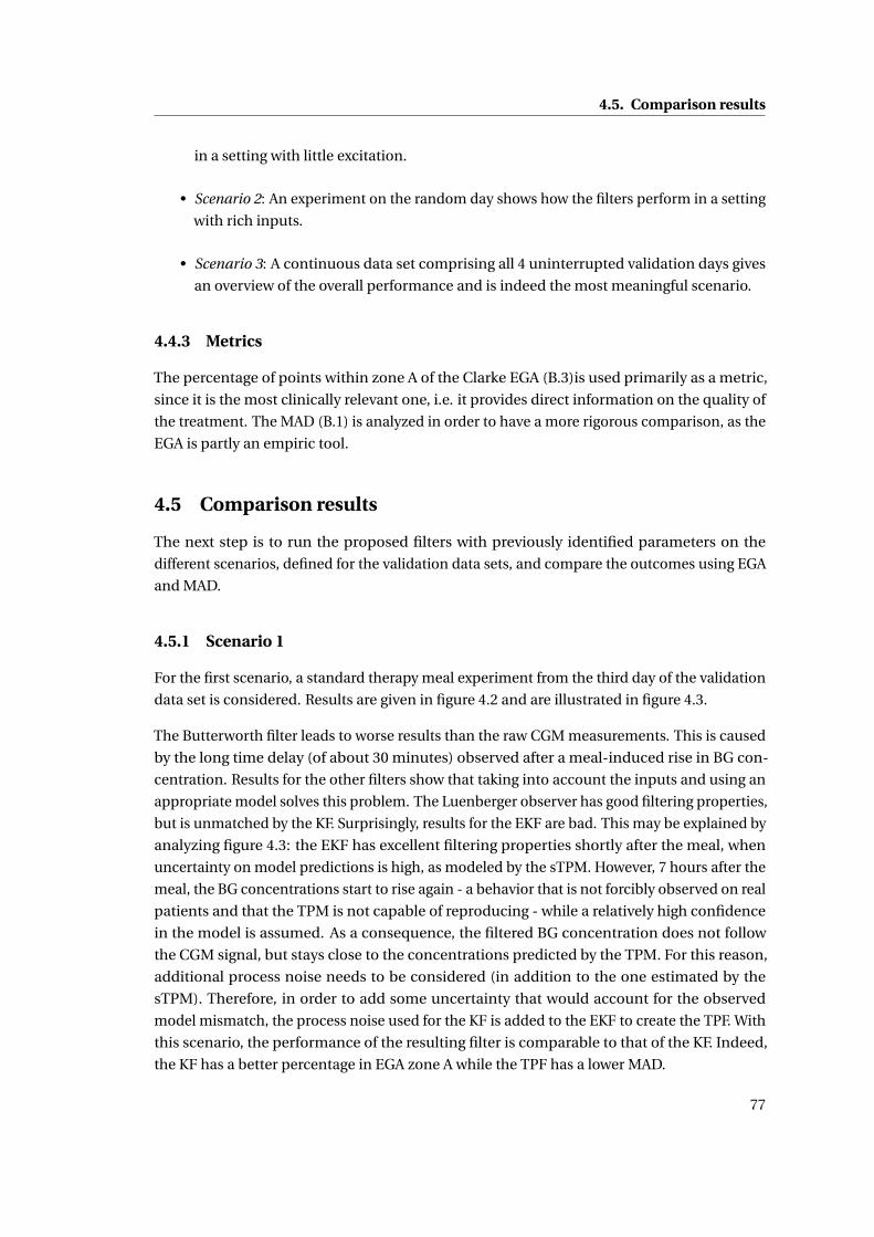
4.5. Comparison results
in a setting with little excitation.
• Scenario 2: An experiment on the random day shows how the filters perform in a setting
with rich inputs.
• Scenario 3: A continuous data set comprising all 4 uninterrupted validation days gives
an overview of the overall performance and is indeed the most meaningful scenario.
4.4.3 Metrics
The percentage of points within zone A of the Clarke EGA (B.3)is used primarily as a metric,
since it is the most clinically relevant one, i.e. it provides direct information on the quality of
the treatment. The MAD (B.1) is analyzed in order to have a more rigorous comparison, as the
EGA is partly an empiric tool.
4.5 Comparison results
The next step is to run the proposed filters with previously identified parameters on the
different scenarios, defined for the validation data sets, and compare the outcomes using EGA
and MAD.
4.5.1 Scenario 1
For the first scenario, a standard therapy meal experiment from the third day of the validation
data set is considered. Results are given in figure 4.2 and are illustrated in figure 4.3.
The Butterworth filter leads to worse results than the raw CGM measurements. This is caused
by the long time delay (of about 30 minutes) observed after a meal-induced rise in BG con-
centration. Results for the other filters show that taking into account the inputs and using an
appropriate model solves this problem. The Luenberger observer has good filtering properties,
but is unmatched by the KF. Surprisingly, results for the EKF are bad. This may be explained by
analyzing figure 4.3: the EKF has excellent filtering properties shortly after the meal, when
uncertainty on model predictions is high, as modeled by the sTPM. However, 7 hours after the
meal, the BG concentrations start to rise again - a behavior that is not forcibly observed on real
patients and that the TPM is not capable of reproducing - while a relatively high confidence
in the model is assumed. As a consequence, the filtered BG concentration does not follow
the CGM signal, but stays close to the concentrations predicted by the TPM. For this reason,
additional process noise needs to be considered (in addition to the one estimated by the
sTPM). Therefore, in order to add some uncertainty that would account for the observed
model mismatch, the process noise used for the KF is added to the EKF to create the TPF. With
this scenario, the performance of the resulting filter is comparable to that of the KF. Indeed,
the KF has a better percentage in EGA zone A while the TPF has a lower MAD.
77
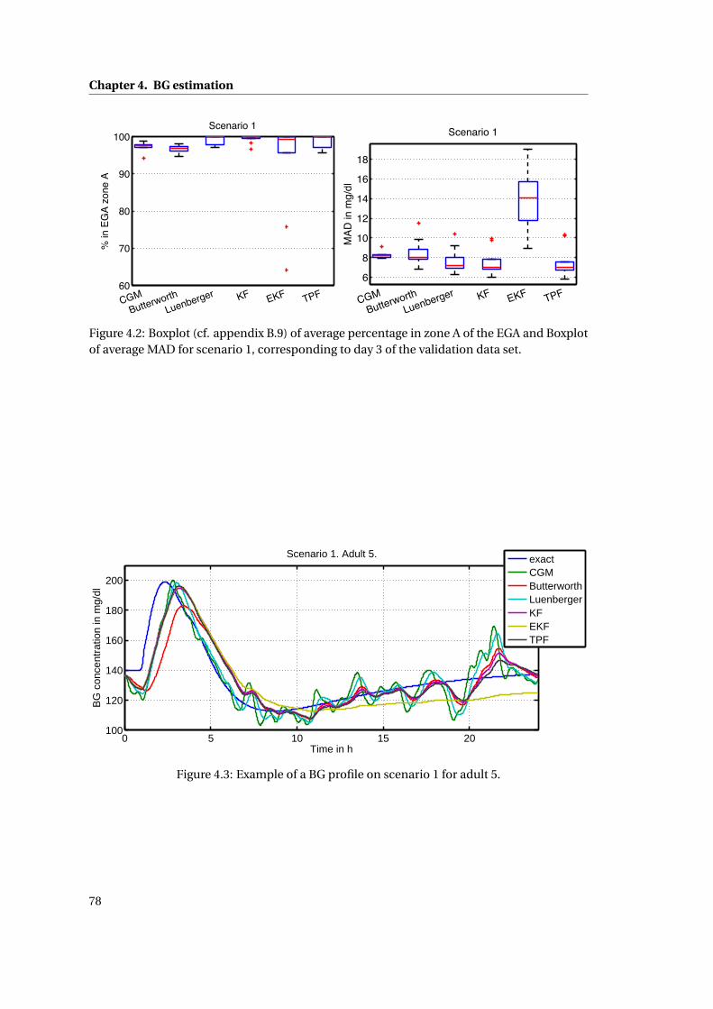
Chapter 4. BG estimation
60
70
80
90
100
CGMButterworth
Luenberger KF EKF TPF
% in
EG
A zo
ne A
Scenario 1
6
8
10
12
14
16
18
CGMButterworth
Luenberger KF EKF TPF
MAD
in m
g/dl
Scenario 1
Figure 4.2: Boxplot (cf. appendix B.9) of average percentage in zone A of the EGA and Boxplotof average MAD for scenario 1, corresponding to day 3 of the validation data set.
0 5 10 15 20100
120
140
160
180
200
Time in h
BG
con
cent
ratio
n in
mg/
dl
Scenario 1. Adult 5.
exactCGMButterworthLuenbergerKFEKFTPF
Figure 4.3: Example of a BG profile on scenario 1 for adult 5.
78
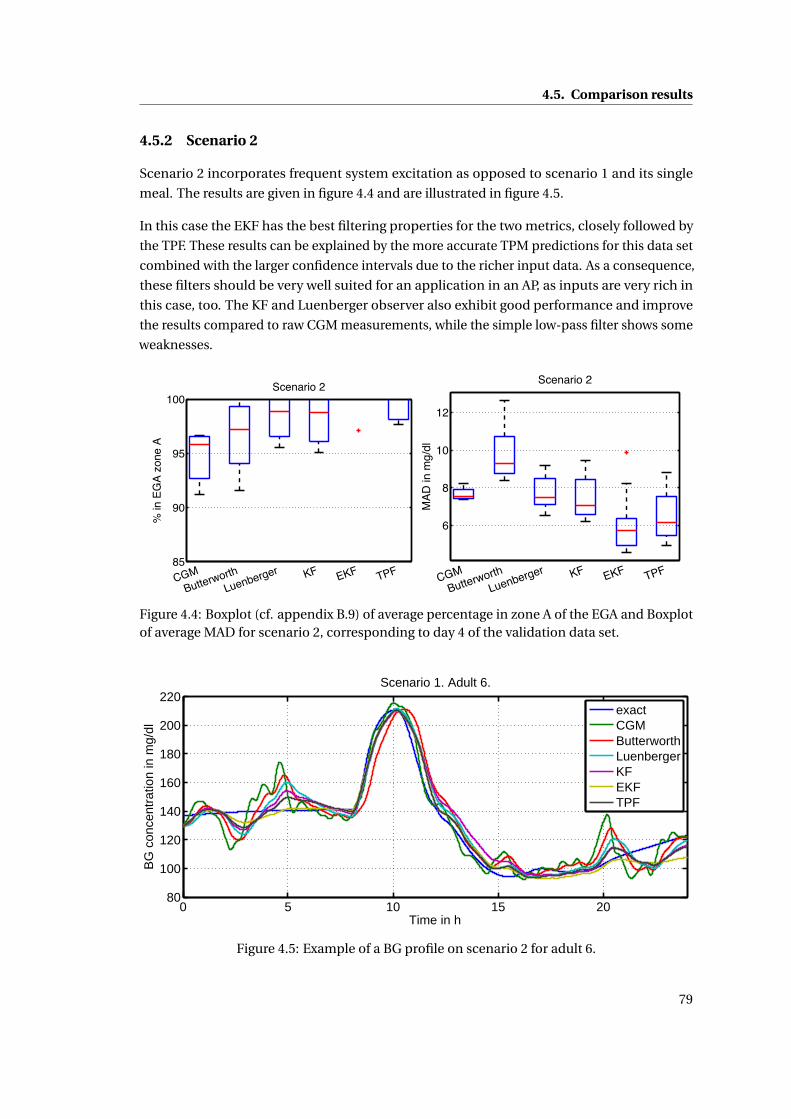
4.5. Comparison results
4.5.2 Scenario 2
Scenario 2 incorporates frequent system excitation as opposed to scenario 1 and its single
meal. The results are given in figure 4.4 and are illustrated in figure 4.5.
In this case the EKF has the best filtering properties for the two metrics, closely followed by
the TPF. These results can be explained by the more accurate TPM predictions for this data set
combined with the larger confidence intervals due to the richer input data. As a consequence,
these filters should be very well suited for an application in an AP, as inputs are very rich in
this case, too. The KF and Luenberger observer also exhibit good performance and improve
the results compared to raw CGM measurements, while the simple low-pass filter shows some
weaknesses.
85
90
95
100
CGMButterworth
Luenberger KF EKF TPF
% in
EG
A zo
ne A
Scenario 2
6
8
10
12
CGMButterworth
Luenberger KF EKF TPF
MAD
in m
g/dl
Scenario 2
Figure 4.4: Boxplot (cf. appendix B.9) of average percentage in zone A of the EGA and Boxplotof average MAD for scenario 2, corresponding to day 4 of the validation data set.
0 5 10 15 2080
100
120
140
160
180
200
220
Time in h
BG
con
cent
ratio
n in
mg/
dl
Scenario 1. Adult 6.
exactCGMButterworthLuenbergerKFEKFTPF
Figure 4.5: Example of a BG profile on scenario 2 for adult 6.
79
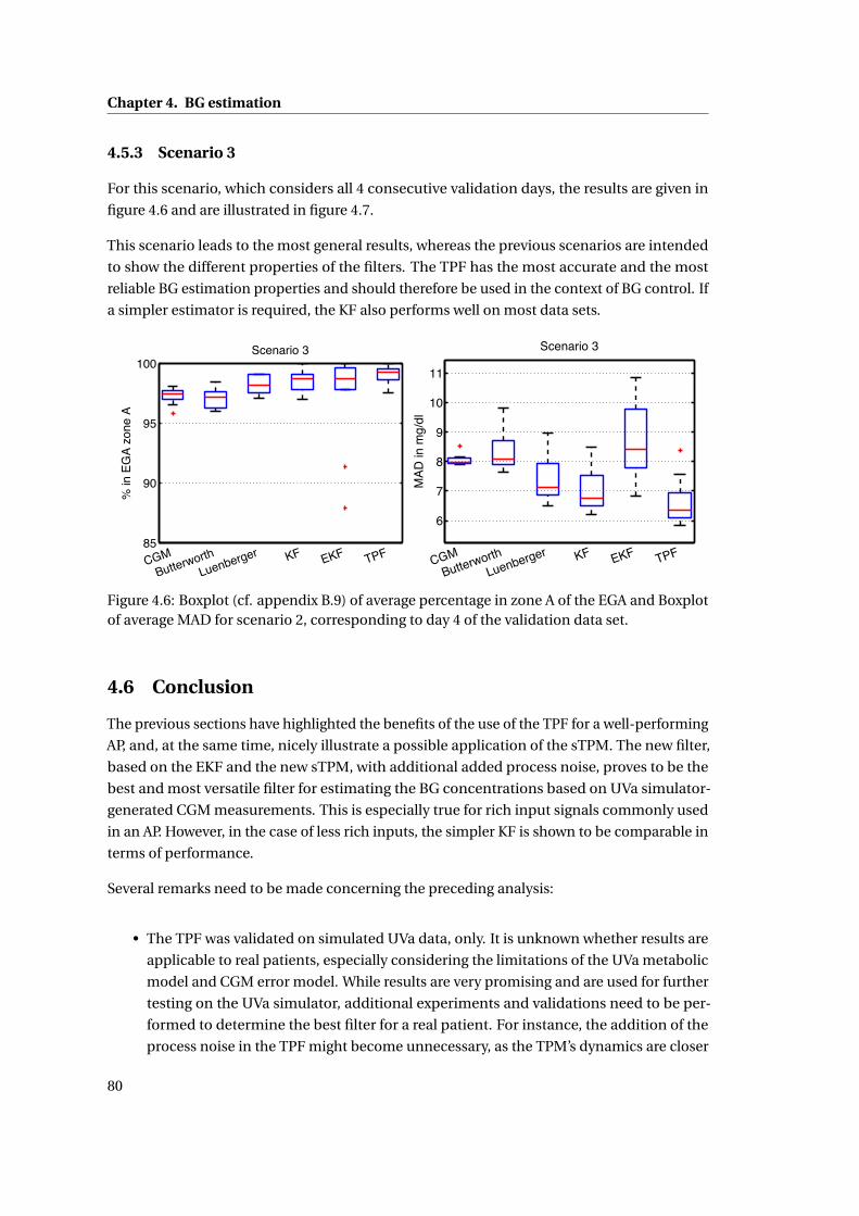
Chapter 4. BG estimation
4.5.3 Scenario 3
For this scenario, which considers all 4 consecutive validation days, the results are given in
figure 4.6 and are illustrated in figure 4.7.
This scenario leads to the most general results, whereas the previous scenarios are intended
to show the different properties of the filters. The TPF has the most accurate and the most
reliable BG estimation properties and should therefore be used in the context of BG control. If
a simpler estimator is required, the KF also performs well on most data sets.
85
90
95
100
CGMButterworth
Luenberger KF EKF TPF
% in
EG
A zo
ne A
Scenario 3
6
7
8
9
10
11
CGMButterworth
Luenberger KF EKF TPF
MAD
in m
g/dl
Scenario 3
Figure 4.6: Boxplot (cf. appendix B.9) of average percentage in zone A of the EGA and Boxplotof average MAD for scenario 2, corresponding to day 4 of the validation data set.
4.6 Conclusion
The previous sections have highlighted the benefits of the use of the TPF for a well-performing
AP, and, at the same time, nicely illustrate a possible application of the sTPM. The new filter,
based on the EKF and the new sTPM, with additional added process noise, proves to be the
best and most versatile filter for estimating the BG concentrations based on UVa simulator-
generated CGM measurements. This is especially true for rich input signals commonly used
in an AP. However, in the case of less rich inputs, the simpler KF is shown to be comparable in
terms of performance.
Several remarks need to be made concerning the preceding analysis:
• The TPF was validated on simulated UVa data, only. It is unknown whether results are
applicable to real patients, especially considering the limitations of the UVa metabolic
model and CGM error model. While results are very promising and are used for further
testing on the UVa simulator, additional experiments and validations need to be per-
formed to determine the best filter for a real patient. For instance, the addition of the
process noise in the TPF might become unnecessary, as the TPM’s dynamics are closer
80
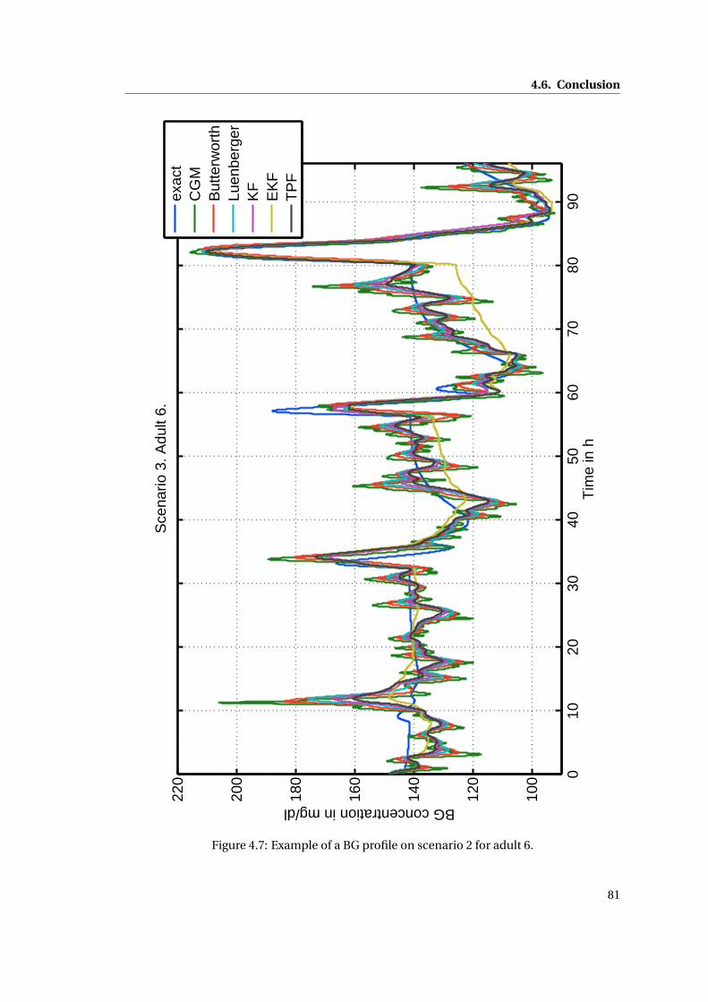
4.6. Conclusion
010
2030
4050
6070
8090
100
120
140
160
180
200
220
Tim
e in
h
BG concentration in mg/dl
Sce
nario
3. A
dult
6.
ex
act
CG
MB
utte
rwor
thLu
enbe
rger
KF
EK
FT
PF
Figure 4.7: Example of a BG profile on scenario 2 for adult 6.
81
Chapter 4. BG estimation
to those of a real patient.
• The proposed TPF relies on meal announcements and insulin infusion profiles. However,
in a real setting, meal announcements may be absent or wrong. In this case, the TPF
would not perform properly anymore and would underestimate the effect of a meal.
While this would lead to lower post-prandial insulin doses using an AP, BG control would
be less effective, but would, nevertheless, remain safe. On the other hand, the TPF can
be used to detect such unannounced meals by determining when the estimated BG
concentration is not consistent with the measured BG concentration anymore. Similarly,
sensor anomalies and unexpected BG excursions can be detected and, thus, necessary
counteractive measures can be taken.
• The measurement noise considered in the TPC is assumed to be white, uncorrelated,
Gaussian noise. However, the noise modeled in the UVa simulator by Breton and
Kovatchev [2008] is clearly correlated. Hence, the use of a KF with correlated noise, as
described by Simon [2006], for example, should be investigated.
• In section 2.5, the initial states of the TPM and the TPM+ were fixed using noisy CGM or
SMBG measurements. The TPF can be used to improve this initialization and potentially
the resulting data fits, parameter correlation, and model predictions.
82
5 BG Control
5.1 Introduction
The central part of T1DM treatment is the control algorithm, which needs to be safe (avoid
hypoglycemia) and perform well (minimize hyperglycemia). Currently, standard therapy
(described in section 2.3.2) is the most common treatment. However, there is room for
improvement for two main reasons.
First, standard treatment does not make full use of the available continuous insulin infusion
capabilities offered by insulin pumps and does not systematically take into account the
information from CGM devices. For this reason, a tremendous research effort for developing
an AP is currently being done and involves a number of institutions funded, for instance, by
the European Commission (AP@home, DIAdvisor), or the JDRF (iAP).
Secondly, the quality of a patient’s treatment depends largely on the patient’s know-how for
the estimation of CHO, and on the willingness to take frequent measurements and calculate
the corresponding insulin doses. For this reason, an automatization procedure requiring
minimal patient involvement could substantially improve the treatment of the patients.
There are two main control approaches to improve T1DM treatment (which were briefly
introduced in section 1.1.2):
• Open-loop control is characterized by the absence of fully automated BG treatment
decisions. The patient or the physician determine and/or validate every insulin injection
and function as a final safety layer. Standard therapy is a form of open-loop control that
has proven to perform with reasonable performance. Nevertheless, improvements in the
form of bolus calculators are being developed and are partially already implemented on
commercial insulin pumps. While these bolus calculators are valuable tools for T1DM
patients, the potential of the insulin pumps and the CGM devices are not fully exploited
so far. For these reasons, a TPM-based open-loop control algorithm is presented and
tested on the UVa simulator.
83
Chapter 5. BG Control
• Closed-loop control is defined by the possibility of the controller to actively take treat-
ment decisions. It is generally characterized by the use of CGM readings to generate
almost continuously adapted insulin infusions. Considering the frequency of the CGM
readings, it is impossible for anyone to validate insulin doses, and the system needs
to be fully autonomous. Only for some variants, patients are required to announce
meals. Despite the huge and prolonged effort to develop an out-patient AP, no device
is commercially available for now. Since the AP has become technically possible with
new CGM augmented insulin pumps, the bottleneck are BG control algorithms and the
strong regulations to certify such potentially harmful devices. The number of proposed
algorithms is large and first versions of closed-loop controllers are being successfully
tested on humans, although a close review reveals that most APs have a large potential
for improvement. In what follows, the TPM is used to design control approaches that
are simple and reliable, and, which are tested on the UVa simulator.
The unavailability of the AP can be explained by the challenges identified in section 1.2. The
inter-patient variability, the meal uptake variability, the complexity of the system, and the
identifiability have already been addressed in this thesis by developing the TPM and the TPM+.
The stochastic model reduces the effects of intra-patient variability, meal announcement
errors, and system complexity, while improving patient safety. The TPF filters part of the
measurement noise without adding time delay. The remaining open issues, which are the
asymmetric control objective, the time delay and the saturation, will be resolved in this chapter,
while patient safety is further improved.
This chapter is organized as follows: First, in section 5.2, the state of the art in open-loop
control is discussed and TPM-based improvements are derived and tested. In section 5.3,
current closed-loop approaches are analyzed and a new controller, the TPC, is designed,
tested, and compared to state-of-the-art controllers. Then, an outlook on other TPM- and
sTPM-based approaches is given in section 5.4, and conclusions are drawn in 5.5.
5.2 Open-loop control
5.2.1 State of the art
Standard therapy as described in section 2.3.2 is a very effective and well accepted open-
loop control strategy. A first step in making this therapy more reliable is to integrate a bolus
calculator into the BG meter. This helps patients with diabetes to compute their insulin bolus
correctly, based on their CF and I2C. Recently, more and more insulin pump manufacturers
have been offering hybrid devices with coupled insulin pump and SMBG (or recently even
CGM) meter. This allows so-called "smart" insulin pumps, which not only compute the
appropriate insulin bolus based on standard therapy, but also verify if no insulin is being
stacked. Insulin stacking occurs when a patient applies standard therapy while there is
still some active insulin in the bloodstream. This is quite likely to happen since even fast-
84
5.2. Open-loop control
acting insulin keeps on acting after several hours. The excess insulin administrated because
of stacking is a very likely cause of hypoglycemia. The currently available smart insulin
pumps use the concept of Insulin On Board (IOB), introduced by Ellingsen et al. [2009], which
quantifies how much insulin is active in the body. This method is effective, but there are
no guidelines to tune the insulin action duration (the only parameter), even though this
parameter may vary significantly from one patient to another. Zisser et al. [2008] give an
overview over current smart insulin pumps.
While smart insulin pumps are simple, yet effective ways to obtain appropriate BG control,
more complex methods potentially lead to improved results and were already explored 15 years
ago by Hejlesen et al. [1997], e.g. . In this context, a model-based optimal control approach is
often adopted, such as proposed by Prud’homme et al. [2011], for which, BG concentrations
are predicted over a prolonged horizon and an insulin infusion profile is computed in order to
minimize a BG-specific cost function. This approach allows optimizing BG control following
various, especially slow or "difficult", meals. However, optimal control-based methods were
shown to lead to inappropriate results, mostly as a result of inappropriate BG prediction
models and unreliable insulin action (cf. 2.4.3).
A first improvement of open-loop control strategies is obtained by using the information
provided by CGM devices. The efficacy of CGM-augmented standard therapy is shown to
improve T1DM treatment to the point of potentially justifying healthcare reimbursement
(Heinemann and Devries [2013]). By using a BG estimator, as discussed in chapter 4, CGM
measurements can also be used to obtain more accurate BG estimations. Vereshchetin et al.
[2013] proposed this approach to treat MDI users, while Patek et al. [2011] applied it in an
optimal control setting. Additionally, the CGM data can be used to generate different alarms
in case of dangerous situations that would typically remain unnoticed otherwise.
Considering the large potential for improvement, in the context of this thesis, open-loop
controllers are designed with the objective of enhancing standard therapy and potentially
taking CGM information into account.
5.2.2 TPM-based open-loop therapy
The main difficulty in designing an optimal control approach in open-loop control is the
choice of an appropriate BG prediction model. For this reason, the TPM, a new prediction
model was developed in chapter 2. In this section a novel open-loop therapy is deduced
directly from the TPM equations, rather than using the TPM for optimization. Because of the
TPM’s simple structure, the optimal treatment can be determined analytically.
Feed-forward meal disturbance rejection
The principle of feed-forward control is to compute current and future system inputs based
on prior knowledge. In this case, this translates to computing the required insulin infusion
85
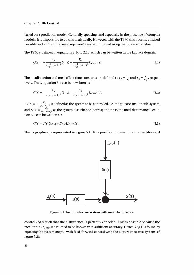
Chapter 5. BG Control
based on a prediction model. Generally speaking, and especially in the presence of complex
models, it is impossible to do this analytically. However, with the TPM, this becomes indeed
possible and an "optimal meal rejection" can be computed using the Laplace transform.
The TPM is defined in equations 2.14 to 2.18, which can be written in the Laplace domain:
G(s) =− Kx
s( 1ax
s +1)2UI (s)+ Kg
s( 1ag
s +1)2UC HO(s). (5.1)
The insulin action and meal effect time constants are defined as τx = 1ax
and τg = 1ag
, respec-
tively. Thus, equation 5.1 can be rewritten as
G(s) =− Kx
s(τx s +1)2 UI (s)+ Kg
s(τg s +1)2 UC HO(s). (5.2)
If I (s) =− Kx
s(τx s+1)2 is defined as the system to be controlled, i.e. the glucose-insulin sub-system,
and D(s) = Kg
s(τg s+1)2 as the system disturbance (corresponding to the meal disturbance), equa-
tion 5.2 can be written as:
G(s) = I (s)Ui (s)+D(s)UC HO(s). (5.3)
This is graphically represented in figure 5.1. It is possible to determine the feed-forward
Figure 5.1: Insulin-glucose system with meal disturbance.
control U0(s) such that the disturbance is perfectly canceled. This is possible because the
meal input UC HO is assumed to be known with sufficient accuracy. Hence, U0(s) is found by
equating the system output with feed-forward control with the disturbance-free system (cf.
figure 5.2):
86
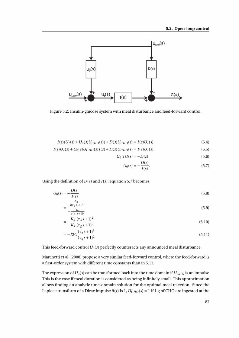
5.2. Open-loop control
Figure 5.2: Insulin-glucose system with meal disturbance and feed-forward control.
I (s)(UI (s)+U0(s)UC HO(s))+D(s)UC HO(s) = I (s)UI (s) (5.4)
I (s)UI (s)+U0(s)UC HO(s)I (s)+D(s)UC HO(s) = I (s)UI (s) (5.5)
U0(s)I (s) =−D(s) (5.6)
U0(s) =−D(s)
I (s). (5.7)
Using the definition of D(s) and I (s), equation 5.7 becomes
U0(s) =−D(s)
I (s)(5.8)
=Kg
s(τg s+1)2
− Kx
s(τx s+1)2
(5.9)
=−Kg
Kx
(τx s +1)2
(τg s +1)2 (5.10)
=−I 2C(τx s +1)2
(τg s +1)2 (5.11)
This feed-forward control U0(s) perfectly counteracts any announced meal disturbance.
Marchetti et al. [2008] propose a very similar feed-forward control, where the feed-forward is
a first-order system with different time constants than in 5.11.
The expression of U0(s) can be transformed back into the time domain if UC HO is an impulse.
This is the case if meal duration is considered as being infinitely small. This approximation
allows finding an analytic time-domain solution for the optimal meal rejection. Since the
Laplace transform of a Dirac impulse δ(t) is 1, UC HO(s) = 1 if 1 g of CHO are ingested at the
87
Chapter 5. BG Control
initial time (t = 0). Using any symbolic computation software, one obtains:
U0(t ) = I 2C
(τ2
x
τ2gδ(t )+ (τg −τx )
(τg t −τx t +2τgτx )
τ4g
e− tτg
)(5.12)
= I 2C
(τ2
x
τ2gδ(t )+ (τg −τx )2
τ4g
te− tτg +2τx
τg −τx
τ3g
e− tτg
)(5.13)
The solution from equations 5.12 and 5.13 needs to be scaled to the total amount of CHO
ingested, when more than 1 g is ingested.
Equation 5.13 consists of three terms:
• The first term is a bolus that is given simultaneously to the meal. It can be observed
that this bolus is smaller than I2C (for δ = 1 g), if insulin action is faster than CHO action
(τx < τg ), the same if the two time constants are identical, and larger if τg < τx .
• The second term is always greater than or equal to 0 and is part of an insulin infusion
profile.
• The third term is positive if τx < τg and negative otherwise. It is the second part of an
insulin infusion profile.
Using the final value theorem, it can be observed that∫ ∞
0 U0(t )d t = I 2C . This means that the
total amount of insulin is always equal to I 2C , the optimal bolus that would have been infused
for standard therapy.
However, depending on the value of q = τxτg
, the ratio of the two time constants, several cases
can be distinguished:
• q < 1: In this case, insulin acts faster than the meal effect and the therapy resulting from
the TPM leads to an initial bolus q · I 2C , smaller than I2C, followed by a positive insulin
infusion profile that perfectly counteracts the meal disturbance.
• q = 1: In this case, insulin action and meal effect have the same time constant and an
optimal bolus at the same time as the meal is enough to counteract the meal disturbance.
In fact the second and third terms of equation 5.13 are 0.
• q > 1: This case is more complex: In fact, the meal acts faster than the insulin, which
entails that it is impossible to perfectly counteract the meal disturbance. Since the
TPM is linear, the optimal profile computed in equation 5.13 leads to an initial bolus
that is greater than I 2C , followed by a partially negative insulin infusion. In fact the
second term of equation 5.12 is negative for 0 < t < 2τxq−1 , where t is the time after
the meal. Since the required insulin infusion becomes negative, this treatment is not
recommended and might become dangerous, because of controller saturation. Indeed,
88
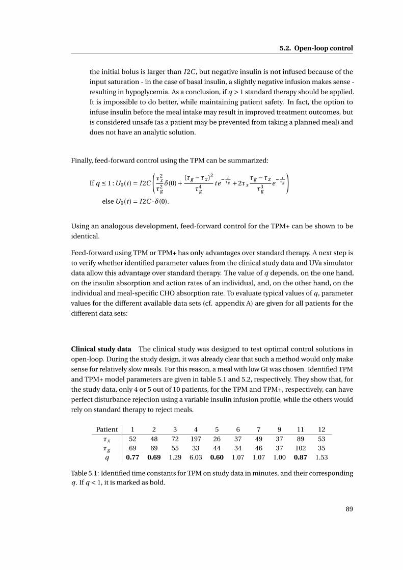
5.2. Open-loop control
the initial bolus is larger than I 2C , but negative insulin is not infused because of the
input saturation - in the case of basal insulin, a slightly negative infusion makes sense -
resulting in hypoglycemia. As a conclusion, if q > 1 standard therapy should be applied.
It is impossible to do better, while maintaining patient safety. In fact, the option to
infuse insulin before the meal intake may result in improved treatment outcomes, but
is considered unsafe (as a patient may be prevented from taking a planned meal) and
does not have an analytic solution.
Finally, feed-forward control using the TPM can be summarized:
If q ≤ 1 : U0(t ) = I 2C
(τ2
x
τ2gδ(0)+ (τg −τx )2
τ4g
te− tτg +2τx
τg −τx
τ3g
e− tτg
)else U0(t ) = I 2C ·δ(0).
Using an analogous development, feed-forward control for the TPM+ can be shown to be
identical.
Feed-forward using TPM or TPM+ has only advantages over standard therapy. A next step is
to verify whether identified parameter values from the clinical study data and UVa simulator
data allow this advantage over standard therapy. The value of q depends, on the one hand,
on the insulin absorption and action rates of an individual, and, on the other hand, on the
individual and meal-specific CHO absorption rate. To evaluate typical values of q , parameter
values for the different available data sets (cf. appendix A) are given for all patients for the
different data sets:
Clinical study data The clinical study was designed to test optimal control solutions in
open-loop. During the study design, it was already clear that such a method would only make
sense for relatively slow meals. For this reason, a meal with low GI was chosen. Identified TPM
and TPM+ model parameters are given in table 5.1 and 5.2, respectively. They show that, for
the study data, only 4 or 5 out of 10 patients, for the TPM and TPM+, respectively, can have
perfect disturbance rejection using a variable insulin infusion profile, while the others would
rely on standard therapy to reject meals.
Patient 1 2 3 4 5 6 7 9 11 12τx 52 48 72 197 26 37 49 37 89 53τg 69 69 55 33 44 34 46 37 102 35q 0.77 0.69 1.29 6.03 0.60 1.07 1.07 1.00 0.87 1.53
Table 5.1: Identified time constants for TPM on study data in minutes, and their correspondingq . If q < 1, it is marked as bold.
89
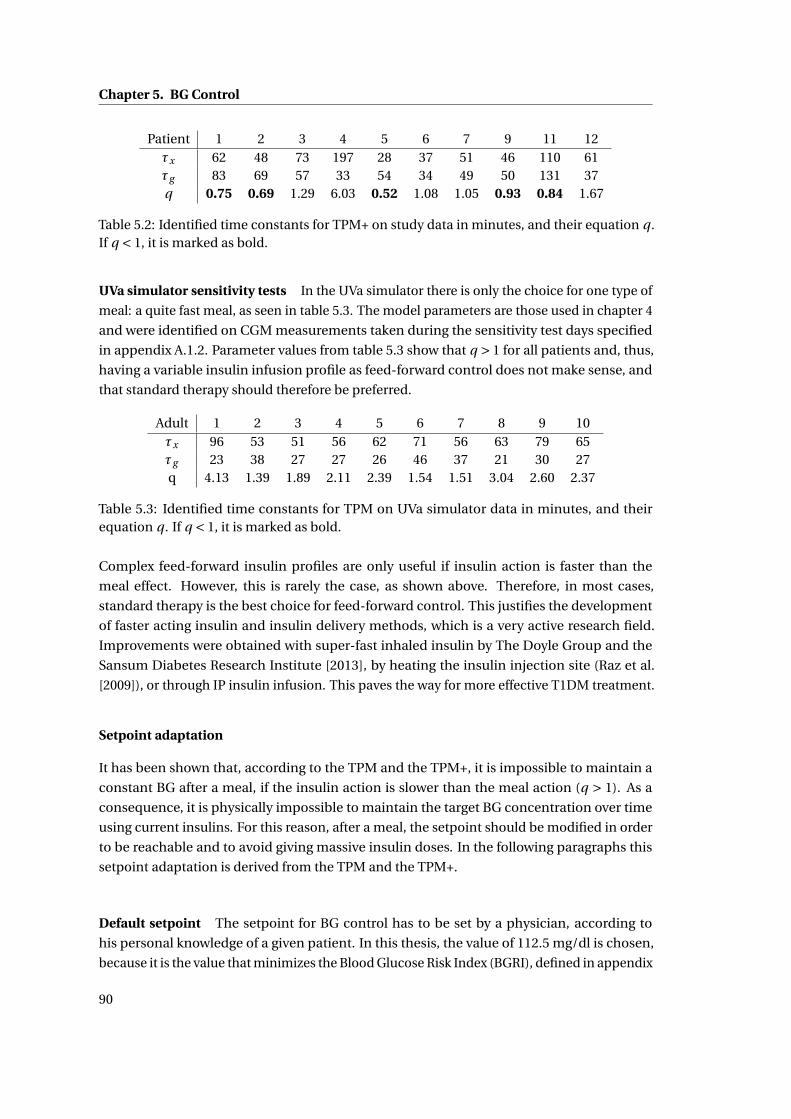
Chapter 5. BG Control
Patient 1 2 3 4 5 6 7 9 11 12τx 62 48 73 197 28 37 51 46 110 61τg 83 69 57 33 54 34 49 50 131 37q 0.75 0.69 1.29 6.03 0.52 1.08 1.05 0.93 0.84 1.67
Table 5.2: Identified time constants for TPM+ on study data in minutes, and their equation q .If q < 1, it is marked as bold.
UVa simulator sensitivity tests In the UVa simulator there is only the choice for one type of
meal: a quite fast meal, as seen in table 5.3. The model parameters are those used in chapter 4
and were identified on CGM measurements taken during the sensitivity test days specified
in appendix A.1.2. Parameter values from table 5.3 show that q > 1 for all patients and, thus,
having a variable insulin infusion profile as feed-forward control does not make sense, and
that standard therapy should therefore be preferred.
Adult 1 2 3 4 5 6 7 8 9 10τx 96 53 51 56 62 71 56 63 79 65τg 23 38 27 27 26 46 37 21 30 27q 4.13 1.39 1.89 2.11 2.39 1.54 1.51 3.04 2.60 2.37
Table 5.3: Identified time constants for TPM on UVa simulator data in minutes, and theirequation q . If q < 1, it is marked as bold.
Complex feed-forward insulin profiles are only useful if insulin action is faster than the
meal effect. However, this is rarely the case, as shown above. Therefore, in most cases,
standard therapy is the best choice for feed-forward control. This justifies the development
of faster acting insulin and insulin delivery methods, which is a very active research field.
Improvements were obtained with super-fast inhaled insulin by The Doyle Group and the
Sansum Diabetes Research Institute [2013], by heating the insulin injection site (Raz et al.
[2009]), or through IP insulin infusion. This paves the way for more effective T1DM treatment.
Setpoint adaptation
It has been shown that, according to the TPM and the TPM+, it is impossible to maintain a
constant BG after a meal, if the insulin action is slower than the meal action (q > 1). As a
consequence, it is physically impossible to maintain the target BG concentration over time
using current insulins. For this reason, after a meal, the setpoint should be modified in order
to be reachable and to avoid giving massive insulin doses. In the following paragraphs this
setpoint adaptation is derived from the TPM and the TPM+.
Default setpoint The setpoint for BG control has to be set by a physician, according to
his personal knowledge of a given patient. In this thesis, the value of 112.5 mg/dl is chosen,
because it is the value that minimizes the Blood Glucose Risk Index (BGRI), defined in appendix
90
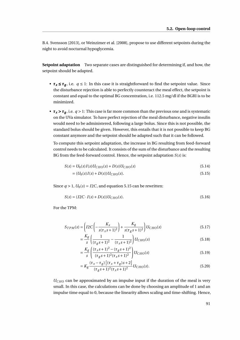
5.2. Open-loop control
B.4. Svensson [2013], or Weinzimer et al. [2008], propose to use different setpoints during the
night to avoid nocturnal hypoglycemia.
Setpoint adaptation Two separate cases are distinguished for determining if, and how, the
setpoint should be adapted.
• τx ≤ τgτx ≤ τgτx ≤ τg , i.e. q ≤ 1: In this case it is straightforward to find the setpoint value. Since
the disturbance rejection is able to perfectly counteract the meal effect, the setpoint is
constant and equal to the optimal BG concentration, i.e. 112.5 mg/dl if the BGRI is to be
minimized.
• τx > τgτx > τgτx > τg , i.e. q > 1: This case is far more common than the previous one and is systematic
on the UVa simulator. To have perfect rejection of the meal disturbance, negative insulin
would need to be administered, following a large bolus. Since this is not possible, the
standard bolus should be given. However, this entails that it is not possible to keep BG
constant anymore and the setpoint should be adapted such that it can be followed.
To compute this setpoint adaptation, the increase in BG resulting from feed-forward
control needs to be calculated. It consists of the sum of the disturbance and the resulting
BG from the feed-forward control. Hence, the setpoint adaptation S(s) is:
S(s) =U0(s)I (s)UC HO(s)+D(s)UC HO(s) (5.14)
= (U0(s)I (s)+D(s))UC HO(s). (5.15)
Since q > 1, U0(s) = I 2C , and equation 5.15 can be rewritten:
S(s) = (I 2C · I (s)+D(s))UC HO(s). (5.16)
For the TPM:
ST P M (s) =(
I 2C
(− Kx
s(τx s +1)2
)+ Kg
s(τg s +1)2
)UC HO(s) (5.17)
= Kg
s
(1
(τg s +1)2 − 1
(τx s +1)2
)UC HO(s) (5.18)
= Kg
s
((τx s +1)2 − (τg s +1)2
(τg s +1)2(τx s +1)2
)UC HO(s) (5.19)
= Kg(τx −τg )
[(τx +τg )s +2
](τg s +1)2(τx s +1)2 UC HO(s). (5.20)
UC HO can be approximated by an impulse input if the duration of the meal is very
small. In this case, the calculations can be done by choosing an amplitude of 1 and an
impulse time equal to 0, because the linearity allows scaling and time-shifting. Hence,
91
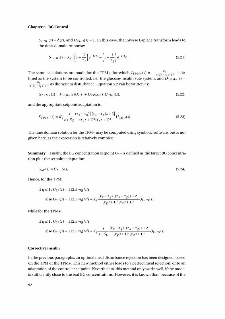
Chapter 5. BG Control
UC HO(t) = δ(t), and UC HO(s) = 1. In this case, the inverse Laplace transform leads to
the time-domain response:
ST P M (t ) = Kg
[(1+ t
τx
)e−t/τx −
(1+ t
τg
)e−t/τg
]. (5.21)
The same calculations are made for the TPM+, for which IT P M+(s) = − Kx
(s+SG )(τx s+1)2 is de-
fined as the system to be controlled, i.e. the glucose-insulin sub-system, and DT P M+(s) =Kg
(s+SG )(τg s+1)2 as the system disturbance. Equation 5.2 can be written as:
GT P M+(s) = IT P M+(s)Ui (s)+DT P M+(s)UC HO(s), (5.22)
and the appropriate setpoint adaptation is:
ST P M+(s) = Kgs
s +SG
(τx −τg )[(τx +τg )s +2
](τg s +1)2(τx s +1)2 UC HO(s). (5.23)
The time domain solution for the TPM+ may be computed using symbolic software, but is not
given here, as the expression is relatively complex.
Summary Finally, the BG concentration setpoint GSP is defined as the target BG concentra-
tion plus the setpoint adaptation:
GSP (s) =Gt +S(s). (5.24)
Hence, for the TPM:
If q ≤ 1 : GSP (s) = 112.5mg /dl
else GSP (s) = 112.5mg /dl +Kg(τx −τg )
[(τx +τg )s +2
](τg s +1)2(τx s +1)2 UC HO(s),
while for the TPM+:
If q ≤ 1 : GSP (s) = 112.5mg /dl
else GSP (s) = 112.5mg /dl +Kgs
s +SG
(τx −τg )[(τx +τg )s +2
](τg s +1)2(τx s +1)2 UC HO(s).
Corrective insulin
In the previous paragraphs, an optimal meal disturbance rejection has been designed, based
on the TPM or the TPM+. This new method either leads to a perfect meal rejection, or to an
adaptation of the controller setpoint. Nevertheless, this method only works well, if the model
is sufficiently close to the real BG concentrations. However, it is known that, because of the
92
5.2. Open-loop control
huge system complexity and uncertainty, the TPM and TPM+ will only lead to an approximate,
yet reliable prediction. For this reason, a corrective insulin dose should be computed at every
insulin injection, using the same concept as in standard therapy (cf. 2.3.2). This corrective
insulin dose UI ,cor r can be improved using the new models, by taking into account the system’s
initial state.
The TPM without the meal sub-model, corresponding to I (s) is given by
G =−Kx X (t ) (5.25)
X (t ) =− 1
τxX (t )+ 1
τxX1(t ) (5.26)
X1(t ) =− 1
τxX1(t )+ 1
τxUI (t ). (5.27)
The Laplace transform with non-zero initial conditions leads to
sG(s) =−Kx X (s)+G0 (5.28)
sX (s) =− 1
τxX (s)+ 1
τxX1(s)+X0 (5.29)
sX1(s) =− 1
τxX1(s)+ 1
τxUI (s)+X1,0, (5.30)
where G0, X0, and X1,0 are the respective initial conditions for the different states.
Hence,
G(s) =−KxX (s)
s+ G0
s(5.31)
X (s) = X1(s)+τx X0
τx s +1(5.32)
X1(s) = UI (s)+τx X1,0
τx s +1. (5.33)
Substituting equation 5.33 into equation 5.32:
X (s) = UI (s)+τx X1,0 +τx (τx s +1)X0
(τx s +1)2 , (5.34)
and substituting equation 5.34 into equation 5.31, the full expression for G , for all initial
conditions, is obtained.
G(s) =−Kx
(UI (s)+τx X1,0 +τx (τx s +1)X0
s(τx s +1)2
)+ G0
s(5.35)
=− Kx
s(τx s +1)2 UI (s)−Kxτx X1,0 +τx (τx s +1)X0
s(τx s +1)2 + G0
s(5.36)
= I (s)UI (s)−τx KxX1,0 + (τx s +1)X0
s(τx s +1)2 + G0
s(5.37)
93
Chapter 5. BG Control
This means that the complete expression for G is the sum of I , the insulin subsystem with
initial conditions set to zero, and two further terms setting the initial conditions.
Next, this expression is used to find the insulin quantity necessary to reach the BG concentra-
tion setpoint. The setpoint should be reached at least when time goes to infinity:
GSP =G(∞). (5.38)
Using the final value theorem:
GSP = lims→0
sG(s) (5.39)
= lims→0
(− Kx
(τx s +1)2 UI (s)−KxτxX1,0 + (τx s +1)X0
(τx s +1)2 +G0
)(5.40)
= Kx (lims→0
UI (s))−Kxτx (X1,0 +X0)+G0. (5.41)
Hence,
lims→0
UI (s) =− 1
Kx(GSP −G0)−τx (X1,0 +X0), (5.42)
and from the definition of the Laplace transform:
lims→0
UI (s) =∫ ∞
0UI (t )d t . (5.43)
Finally,∫ ∞
0UI (t )d t =− 1
Kx(GSP −G0)−τx (X1,0 +X0). (5.44)
This means that, according to the TPM, the total amount of insulin that needs to be adminis-
tered in order to reach the BG concentration setpoint is composed of two terms:
1. the difference between the setpoint and current BG concentration divided by Kx (which
is the same as the C F ), which corresponds exactly to the correction term of standard
therapy.
2. the opposite of the sum of X and X1 at the initial time, multiplied by the insulin time
constant τx . The next step is to show how these initial values of X and X1 can be
estimated using insulin infusion history.
X and X1 are taken from the Laplace transform of the TPM equations:
X (s) = X1(s)
τx s +1(5.45)
X1(s) = UI (s)
τx s +1. (5.46)
94
5.2. Open-loop control
Thus,
X (s)+X1(s) = X1(s)
τx s +1+ UI (s)
τx s +1(5.47)
= UI (s)
(τx s +1)2 + UI (s)
τx s +1(5.48)
= τx s +2
(τx s +1)2 UI (s). (5.49)
Therefore, in Laplace domain, the second term of equation 5.44 corresponds to:
τx (X (s)+X1(s)) = τ2x s +2τx
(τx s +1)2 UI (s), (5.50)
and is evaluated at time t = 0 using past insulin injections information.
Finally, the quantity of corrective insulin to be injected at time t = 0 is
UI ,cor r =− 1
Kx(GSP −G0)−τx (X1,0 +X0), (5.51)
because, considering the dynamics of the TPM that make insulin overshoots impossible,
the fastest way to reach the setpoint BG concentration is by infusing the insulin as early as
possible.
The same calculation cannot be done for the TPM+. In fact,∫ ∞
0UI (t )d t =−∞, (5.52)
because the TPM+ converges to 0 if times goes to infinity. Hence, a constant negative insulin
infusion would be required after some time. Nevertheless, using UI ,cor r in the context of the
TPM+ can still be recommended, as long as SG is sufficiently small.
Insulin on board
IOB is a concept that was introduced by Ellingsen et al. [2009], and was already described in
the state of the art in section 5.2.1. There are several methods to predict how much insulin
stays active in the bloodstream after a given time. They range from linear to non-linear curves,
but almost all rely on a single time constant. The difficulty is to estimate this time constant
such that a compromise between performance and safety is obtained. For this reason, it is
proposed to use the TPM to evaluate the IOB, based on the identified model parameters. IOB
is the amount of injected insulin UI (s)s , minus the insulin that has already acted − I (s)
Kx·UI (s),
95
Chapter 5. BG Control
corresponding to the drop in BG divided by the insulin sensitivity:
IOB(s) = UI (s)
s+ I (s)
Kx·UI (s) (5.53)
=(
1
s− 1
s(τx s +1)2
)·Ui (s) (5.54)
Thus,
IOB(s)
UI (s)=
(1
s− 1
s(τx s +1)2
)(5.55)
= τ2x s2 +2τx s
s(τx s +1)2 (5.56)
= τ2x s +2τx
(τx s +1)2 (5.57)
This value corresponds exactly to the expression of the right hand side term of equation 5.50
and corresponds to the second term of the corrective insulin UI ,cor r that can now be written
as
UI ,cor r =− 1
Kx(GSP −G0)− IOB(0), (5.58)
where IOB(0) is the insulin on board at the initial time. It should be noticed that IOB only
depends on the time constant τx .
Open-loop control summary
An open-loop control strategy was derived from the TPM, leading to an optimization-free,
model-based treatment that augments standard therapy by adding safety and performance
enhancements, and does not rely on CGM. This treatment will be referred to as the Therapy
Parameter-based Controller in Open-Loop (TPC OL).
It is composed of 3 new parts that are added to standard therapy:
1. Meal disturbances are rejected by the following feed-forward control administered after
the meal intake time and multiplied by the mass of ingested CHO:
If q ≤ 1 : U0(t ) = I 2C
(τ2
x
τ2gδ(t )+ (τg −τx )2
τ4g
te− tτg +2τx
τg −τx
τ3g
e− tτg
)else U0(t ) = I 2C ·δ(t ).
This enhances performance, especially in the case of a slow meal (q < 1).
2. The BG concentration setpoint is adapted by adding the term S(s) to the target BG
96
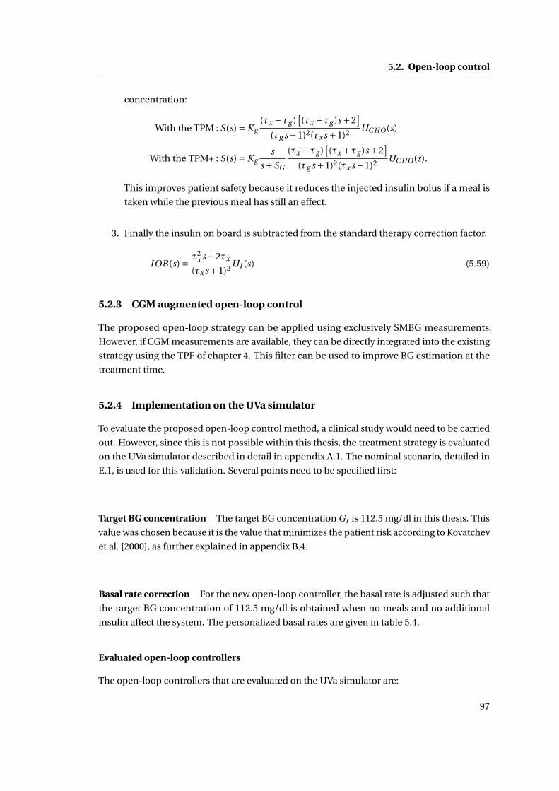
5.2. Open-loop control
concentration:
With the TPM : S(s) = Kg(τx −τg )
[(τx +τg )s +2
](τg s +1)2(τx s +1)2 UC HO(s)
With the TPM+ : S(s) = Kgs
s +SG
(τx −τg )[(τx +τg )s +2
](τg s +1)2(τx s +1)2 UC HO(s).
This improves patient safety because it reduces the injected insulin bolus if a meal is
taken while the previous meal has still an effect.
3. Finally the insulin on board is subtracted from the standard therapy correction factor.
IOB(s) = τ2x s +2τx
(τx s +1)2 UI (s) (5.59)
5.2.3 CGM augmented open-loop control
The proposed open-loop strategy can be applied using exclusively SMBG measurements.
However, if CGM measurements are available, they can be directly integrated into the existing
strategy using the TPF of chapter 4. This filter can be used to improve BG estimation at the
treatment time.
5.2.4 Implementation on the UVa simulator
To evaluate the proposed open-loop control method, a clinical study would need to be carried
out. However, since this is not possible within this thesis, the treatment strategy is evaluated
on the UVa simulator described in detail in appendix A.1. The nominal scenario, detailed in
E.1, is used for this validation. Several points need to be specified first:
Target BG concentration The target BG concentration Gt is 112.5 mg/dl in this thesis. This
value was chosen because it is the value that minimizes the patient risk according to Kovatchev
et al. [2000], as further explained in appendix B.4.
Basal rate correction For the new open-loop controller, the basal rate is adjusted such that
the target BG concentration of 112.5 mg/dl is obtained when no meals and no additional
insulin affect the system. The personalized basal rates are given in table 5.4.
Evaluated open-loop controllers
The open-loop controllers that are evaluated on the UVa simulator are:
97
Chapter 5. BG Control
Adult UI ,b in U/h1 1.5002 1.6003 1.7334 1.0485 1.6836 1.8507 1.4508 1.3969 1.450
10 1.501
Table 5.4: Adjusted basal rates to have a Gss of 112.5 mg/dl.
UVa simulator standard therapy (UVa ST) The results from the new open-loop strategy are
tested against the standard open-loop algorithm implemented by default in the UVa simulator.
The basal rate is the predefined basal rate that keeps the unperturbed subject at a given basal
BG concentration, which is around 140 mg/dl (cf. A.1). The meal bolus is given by multiplying
the given I2C with the amount of ingested CHO. No corrective insulin is injected. This means
that this method is fully open-loop, since it does not rely on any measurements at all.
Standard therapy based on TPM parameters (TPM ST) UVa ST is not the standard therapy
described in 2.3.2, because no corrective insulin is given. For this reason, standard therapy
using the parameters identified with the TPM and the adjusted basal rate are applied to the
UVa simulator. This should indicate how standard therapy performs on the UVa simulator. It
should be noted that there is still a difference compared to the original standard therapy in
that, on the simulator, CGM measurements are used instead of SMBG measurements. This
should have a negative effect on performance, as CGM is less accurate than SMBG. The model
parameters result from the sensitivity tests described in A.1.2 and were already used in chapter
4.
TPM-based open-loop control (TPC OL) The TPC OL is constructed as in 5.2.2. The same
parameter set than for the TPM ST is used. Again, simulated CGM measurements are used,
since no SMBG measurements are available in the UVa simulator.
TPM-based open-loop control with TPF (TPC TPF-OL) This controller is the same as the
TPC OL, with the exception that the TPF is used for estimating BG concentrations, instead of
using raw CGM data.
98
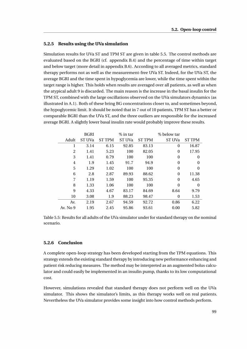
5.2. Open-loop control
5.2.5 Results using the UVa simulation
Simulation results for UVa ST and TPM ST are given in table 5.5. The control methods are
evaluated based on the BGRI (cf. appendix B.4) and the percentage of time within target
and below target (more detail in appendix B.6). According to all averaged metrics, standard
therapy performs not as well as the measurement-free UVa ST. Indeed, for the UVa ST, the
average BGRI and the time spent in hypoglycemia are lower, while the time spent within the
target range is higher. This holds when results are averaged over all patients, as well as when
the atypical adult 9 is discarded. The main reason is the increase in the basal insulin for the
TPM ST, combined with the large oscillations observed on the UVa simulators dynamics (as
illustrated in A.1). Both of these bring BG concentrations closer to, and sometimes beyond,
the hypoglycemic limit. It should be noted that in 7 out of 10 patients, TPM ST has a better or
comparable BGRI than the UVa ST, and the three outliers are responsible for the increased
average BGRI. A slightly lower basal insulin rate would probably improve these results.
BGRI % in tar % below tarAdult ST UVa ST TPM ST UVa ST TPM ST UVa ST TPM
1 3.14 6.15 92.85 83.13 0 16.872 1.41 5.23 100 82.05 0 17.953 1.41 0.79 100 100 0 04 1.9 1.45 91.7 94.9 0 05 1.29 1.02 100 100 0 06 2.8 2.87 89.93 88.62 0 11.387 1.19 1.59 100 95.35 0 4.658 1.33 1.06 100 100 0 09 4.33 4.67 83.17 84.69 8.64 9.79
10 3.08 1.9 88.23 98.47 0 1.53Av. 2.19 2.67 94.59 92.72 0.86 6.22
Av. No 9 1.95 2.45 95.86 93.61 0.00 5.82
Table 5.5: Results for all adults of the UVa simulator under for standard therapy on the nominalscenario.
5.2.6 Conclusion
A complete open-loop strategy has been developed starting from the TPM equations. This
strategy extends the existing standard therapy by introducing new performance enhancing and
patient risk reducing measures. The method may be interpreted as an augmented bolus calcu-
lator and could easily be implemented in an insulin pump, thanks to its low computational
cost.
However, simulations revealed that standard therapy does not perform well on the UVa
simulator. This shows the simulator’s limits, as this therapy works well on real patients.
Nevertheless the UVa simulator provides some insight into how control methods perform.
99
Chapter 5. BG Control
5.3 Closed-loop control
5.3.1 State of the art
A detailed review of existing closed-loop control methods is not be given here, as the number
of such algorithms and related simulation and clinical studies is huge. The aim of this section
is rather to introduce the different available options for the design of an AP algorithm and
to give examples. This will justify the choices made and the goals set for the design of the
proposed control algorithms.
For a more detailed review, the interested reader is referred to recent works by Lunze et al.
[2012] for a technical review, or by Bequette [2012] for a broader overview. Cobelli et al. [2011]
review the past efforts in designing an AP, introduce the current projects and give an outlook
on future works. Renard et al. [2013] make an update of recent progress in the development of
an AP, with focus on the advances in out-patient studies.
In the following paragraphs, different aspects of closed-loop BG control are discussed and
recent examples are given.
Degree of automation
According to the definition of closed-loop control in this thesis (cf. section 5.1), an AP is a
device that takes control actions without previous patient interaction. Therefore, there are
many different degrees of automation and complexity that define several classes of APs.
Pump suspension algorithms are probably the most simple and intuitive forms of an AP. These
algorithms shut of the basal insulin infusion if certain conditions such as the passing of a low
BG concentration threshold, or hypoglycemia predictions, are met. Devices with automated
pump shutoff are currently on the market, and have recently been approved by the FDA. For
this reason, the manufacturer, Medtronic [2013], is marketing their pump suspend algorithm
as "the world’s first breakthrough in Artificial Pancreas technology". This very simple solution
(even though more complex variations, such as proposed by Cameron et al. [2012], for example,
exist) is only a first step towards reaching the full potential of an AP.
A next degree of automation are overnight BG controllers that control nocturnal BG con-
centrations and actively administer insulin when required. BG concentrations are easier to
manage overnight than during the day, as no major system disturbances occur. Overnight
controllers are currently being investigated and many studies have recently been published,
such as those by Elleri et al. [2011], by O’Grady et al. [2012], by Capel et al. [2013], or by Nimri
et al. [2013].
A further degree in automation is reached using a full AP with meal announcements, meaning
that insulin infusion is completely automatized and the patient only provides information on
his meal intakes and, possibly, on his physical activity. As a consequence, the involvement is
100
5.3. Closed-loop control
the same as with a standard therapy, but the treatment quality is potentially improved. This is
the most common type of AP currently investigated.
A fully automated AP is the last step in the development of closed-loop control. In this case,
the patient does not have to take any action at all - as if he had an artificial pancreas. These
controllers should eventually reproduce the functionality of a healthy pancreas and allow
patients with T1DM to live their lives without the limitations of diabetes. Unfortunately, with
the current limitations of the SC-SC route and its resulting time delays, the performance of a
healthy pancreas cannot be reached.
Type of controller
The type of controller is an important choice to make for the design of an AP. A short overview
is given below.
Proportional-Integral-Derivative (PID) controller The classical PID controller is by far the
most used controller and is often applied for BG control, as well. Many PID tuning methods
exist - the recent variants by Weinzimer et al. [2008], or by Lee et al. [2013] should be noted. The
PID is a very simple and well-accepted controller that has a few important drawbacks, when
it comes to resolving the challenges in BG control of section 1.2. Indeed, the PID controller
is not well suited for systems with large time delays (1.2.6), or with control saturation (1.2.7).
Additionally, the PID controller is designed for symmetric problems, which makes safe control
more difficult (1.2.5) and requires robust design methods, resulting in reduced performance.
However, PID controllers may give acceptable results, if appropriate feed-forward is applied
and no large, unexpected BG excursions occur.
Model Predictive Control (MPC) MPC is the most promising control algorithm for the use
in BG control. It allows considering constraints, saturations, asymmetric control objectives,
and non-linear models. MPC has none of the drawbacks of the PID controller. This explains
why MPC is currently the most used for BG controller and is implemented in various forms as
illustrated by the following recent examples:
• Soru et al. [2012] use a linear unconstrained MPC using the linearized Dalla Man model
• Zarkogianni et al. [2011] use an adaptive non-linear MPC
• Grosman et al. [2011] introduce a multi-zone MPC that has a different behavior depend-
ing on the patient’s glycemia
• Cameron et al. [2011] model the prediction uncertainty and use it to minimize patient
risk.
101
Chapter 5. BG Control
With MPC, an optimization problem is solved at every sampling time. A given cost function
is minimized in order to compute optimal insulin infusions. This cost function relies on
model-based predictions and is generally minimized under constraints, e.g. saturation.
However, as promising as the MPC concept is, results still lag behind expectations. The main
reason is the lack of appropriate prediction models - the most critical part in MPC - as will be
explained below. Another drawback is that MPC is computationally expensive, and the price
increases with the number of constraints, model non-linearities, and model order.
Other controllers Many other approaches are being tried for BG control, but are used much
less. Examples are Error Dynamics Shaping (EDS) proposed by Cormerais and Richard [2012],
fuzzy logic used by Miller et al. [2011] or partially by Zarkogianni et al. [2011], or robust
methods, such as sliding mode control, as described by Abu-Rmileh and Garcia-Gabin [2012].
Choosing the model
Almost all of the applied methods are, to some extent, model-based. Therefore, the crucial
question on what model to use arises. The different available models were discussed in detail
in 2.2.3. The impact of an inappropriate prediction model was experienced by Dassau et al.
[2012], whose MPC only gave benign insulin infusions because of an IOB safety measure.
Another example is the MPC by Soru et al. [2012] that needs therapy parameter-based feed-
forward control to work properly - which contradicts the concept of the MPC. In fact, the
model of an MPC should give appropriate insulin doses, even in the presence of a meal. If
feed-forward is used, a much simpler controller is typically sufficient.
In some cases, the model is not identifiable on BG measurements only, or appropriate training
data is not available. Population model parameters can be used in this case, or, as proposed by
Soru et al. [2012], the cost function may be personalized. Considering the large inter-patient
variability, these solutions are generally sub-optimal and should therefore only be used if
personalized model parameters cannot be obtained.
Meal announcements
Currently, T1DM patients always need to estimate the CHO content of meals and deduce
the amount of insulin to infuse. When designing an AP, one needs to decide whether the
AP should to do this task itself. Meal announcements go hand in hand with feed-forward
control, while unannounced meals are more difficult to reject and lead to higher postpran-
dial BG concentration peaks. If meals are not announced, meal detection algorithms (e.g.
citeBoiroux2010a), or probabilistic meal predictors (e.g. Hughes et al. [2010]), can lead to
better BG control. Weinzimer et al. [2008], or Campetelli et al. [2013] consider the option to
infuse feed-forward insulin 15 or 60 minutes before the meal, respectively. If the ingested meal
has a high GI (i.e. a fast meal), this improves results even further, but increases the risk of
102
5.3. Closed-loop control
hypoglycemia, if the meal is finally not taken.
Adaptive methods
Adaptive methods are used for two main different purposes, i.e. either to account for the shift
in parameter values that naturally occurs over time, or to reject disturbances. The first case
can be done by methods such as run-to-run (R2R), as investigated by François et al. [2003], or
Daskalaki et al. [2012]. In this case, parameters only change slowly with time constants of the
order of days. This is an important feature that makes frequent re-identifications of model
parameters useless and improves treatment quality. However, the changes in parameters need
to be closely monitored to avoid safety problems. In the second case, the time constant of
parameter changes are much shorter and parameters may vary significantly in a very short
time. Such a method is proposed by Turksoy et al. [2013], for instance. Zarkogianni et al.
[2011] adapt MPC parameters using NN and fuzzy logic when model predictions are no longer
accurate. Since parameters change in the order of minutes, it is impossible to check the validity
of parameters, thus adding another risk factor to the treatment.
Controller validation
The ideal way to evaluate the performance of a controller is to do a clinical study. Some
MPCs were recently tested within the context of large scale projects, such as AP@home, the
iAP project, or others (Elleri et al. [2012], Dassau et al. [2012], Luijf et al. [2013]). Even the
feasibility of out-patient AP use (Kovatchev et al. [2013]), or closed-loop control for T2DM
(Kumareswaran et al. [2013]), is being explored. Unfortunately, most researchers do not have
the funds and the expertise to do clinical studies. For this reason, the UVa simulator, described
in appendix A.1, is an alternative to showcase the potential of a given control algorithm. Many
simulation studies were done either on the 100- or the 10-patient population, and published.
Nevertheless, these results are only an indicator for potentially good results and clinical studies
are still required to validate the most promising methods.
Conclusion of the state of the art: BG control goals
Designing a controller for diabetes treatment involves making choices beforehand. In the
previous section, some of the most important aspects were introduced. Considering the
advantages and disadvantages of these different points, this thesis aims at finding or designing
the "best" control method, based on the TPM that was specifically developed for this use
in chapter 2. The controller should be able to handle scenarios with announced and unan-
nounced meals. In other words, control should be better if a patients announces his meal,
but is should remain acceptable whenever he does not. For the time being, a method with
fixed parameters is considered, but can be extended to an adaptive scheme, with large time
constants. As a clinical study is not possible within this small-scale project, the proposed
103
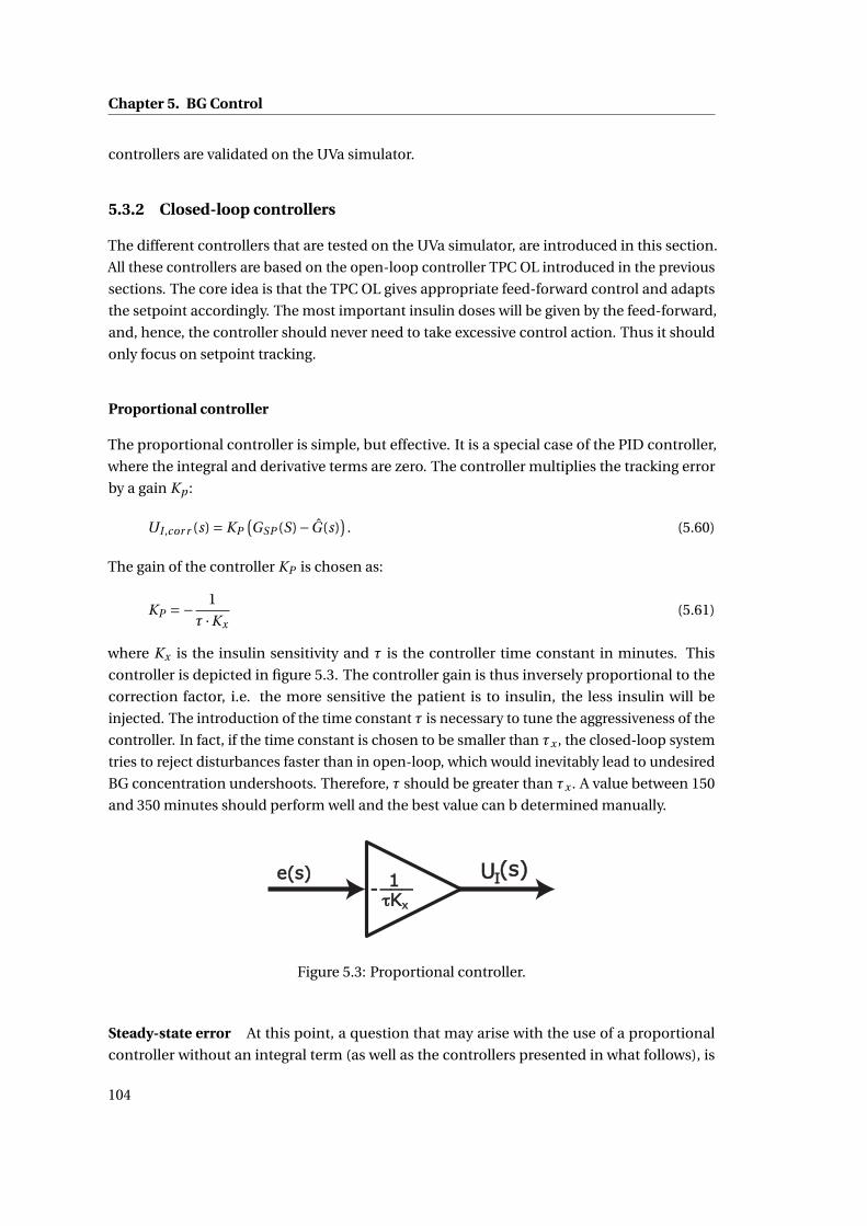
Chapter 5. BG Control
controllers are validated on the UVa simulator.
5.3.2 Closed-loop controllers
The different controllers that are tested on the UVa simulator, are introduced in this section.
All these controllers are based on the open-loop controller TPC OL introduced in the previous
sections. The core idea is that the TPC OL gives appropriate feed-forward control and adapts
the setpoint accordingly. The most important insulin doses will be given by the feed-forward,
and, hence, the controller should never need to take excessive control action. Thus it should
only focus on setpoint tracking.
Proportional controller
The proportional controller is simple, but effective. It is a special case of the PID controller,
where the integral and derivative terms are zero. The controller multiplies the tracking error
by a gain Kp :
UI ,cor r (s) = KP(GSP (S)−G(s)
). (5.60)
The gain of the controller KP is chosen as:
KP =− 1
τ ·Kx(5.61)
where Kx is the insulin sensitivity and τ is the controller time constant in minutes. This
controller is depicted in figure 5.3. The controller gain is thus inversely proportional to the
correction factor, i.e. the more sensitive the patient is to insulin, the less insulin will be
injected. The introduction of the time constant τ is necessary to tune the aggressiveness of the
controller. In fact, if the time constant is chosen to be smaller than τx , the closed-loop system
tries to reject disturbances faster than in open-loop, which would inevitably lead to undesired
BG concentration undershoots. Therefore, τ should be greater than τx . A value between 150
and 350 minutes should perform well and the best value can b determined manually.
Figure 5.3: Proportional controller.
Steady-state error At this point, a question that may arise with the use of a proportional
controller without an integral term (as well as the controllers presented in what follows), is
104
5.3. Closed-loop control
whether there is steady-state error, i.e. a difference between setpoint and BG concentration
when the closed-loop system is at steady state. As explained by Longchamp [2010], steady-
state error is zero, if the type of the open-loop system K (s)H(s) is greater or equal than one.
The type is defined as the number of integrators in the transfer function, where K (s) is the
transfer function of the controller and H (s) is the open-loop transfer function of the controlled
system. If H(s) corresponds to the TPM:
K (s)H(s) = KP I (s) (5.62)
=−KPKx
s(τx s +1)2 , (5.63)
which contains an integral term 1s and, hence, there will not be any steady-state error. However,
the real patient dynamics are sometimes closer to the TPM+ dynamics and in that case:
K (s)H(s) =−KPKx
(s +SG )(τx s +1)2 (5.64)
whose type is 0, potentially leading to steady-state errors. The same goes for an application on
the UVa simulator that does not have integral dynamics, either. To get rid of the steady-state
error, an integrator term could be added to the controller. However, this leads to decreased
controller robustness and the control saturation possibly leads to integral windup. An anti-
reset windup helps in the latter case, but the decreased patient safety does not justify the use
of an integral term.
Finally, this approach does not eliminate the steady-state error, it, however, reduces its effect.
The key is that, if feed-forward control at steady-state is set to maintain the BG concentration
at the target, then steady-state error is zero at this target BG. In other words, there will be no
steady-state error at the target BG, if basal insulin infusion is set to stabilize the patient at this
concentration. This can easily be done on the UVa simulator through the choice of the basal
rate (cf. table 5.4). For real patient data, this is more difficult as a physician needs to tune
the basal rate, or it can set by more complex methods, such as R2R proposed by Palerm et al.
[2008].
Therapy Parameter-based Controller (TPC)
Concept description The TPC is a new control algorithm that is directly inspired by standard
therapy and, more specifically, by the concept of the corrective bolus. In standard therapy,
at certain times, such as before meals, BG concentration is measured and, according to the
difference to the target BG, corrective insulin UI ,cor r (t) is administered. As described in
section 2.3.2, this corrective bolus is computed as:
UI ,cor r (t ) = e(t )
Kx, (5.65)
105
Chapter 5. BG Control
where e is the difference between the setpoint and the measured BG. The idea of the TPC is to
apply this treatment, not only at specific times, but at every sampling time (or continuously).
In other words this leads to a proportional controller with gain 1Kx
. Of course, the application
of this controller can be dangerous:
• The controller gain is large compared to other PID controllers. This will most likely lead
to BG concentration undershoots.
• Negative insulin boluses are only possible to a very limited extent, depending on the
basal insulin infusion. Larger negative boluses cannot be administered and control
needs to avoid any BG concentration undershoots to maintain patient safety.
• This controller does not account for the time delays (∼ 20 min) in insulin action. This
can lead to insulin stacking, where full correction boluses are given despite active insulin
being on board. This is a serious issue, even for patients following standard therapy, and
is unacceptable for the described controller.
To prevent this insulin stacking, the TPM allows estimating by how much BG concentration is
expected to drop, using the IOB introduced in 5.2:
IOB(s) = τ2x s +2τx
(τx s +1)2 UI (s) (5.66)
The transfer function to compute IOB is defined as:
HIOB (s) = τ2x s +2τx
(τx s +1)2 . (5.67)
Now, to obtain the TPC, the computed insulin amount is reduced by the amount of active
insulin:
UI (s) = e(s)
Kx−HIOB (s)UI (s) (5.68)
(1+HIOB (s))UI (s) = e(s)
Kx(5.69)
UI (s) = e(s)
Kx (1+HIOB (s)). (5.70)
The TPC, which is depicted in figure 5.4, can also be interpreted as a closed-loop version of
the TPC OL that is evaluated at specified sampling times. The estimation of the current BG
may come directly from the CGM device, or may be filtered by the TPF, depending on what
information is available. IOB can be estimated using the TPF and equation 5.71, which results
in an estimate that is corrected by CGM measurements.
IOB(s) = τx (X (s)+ X1(s)), (5.71)
106
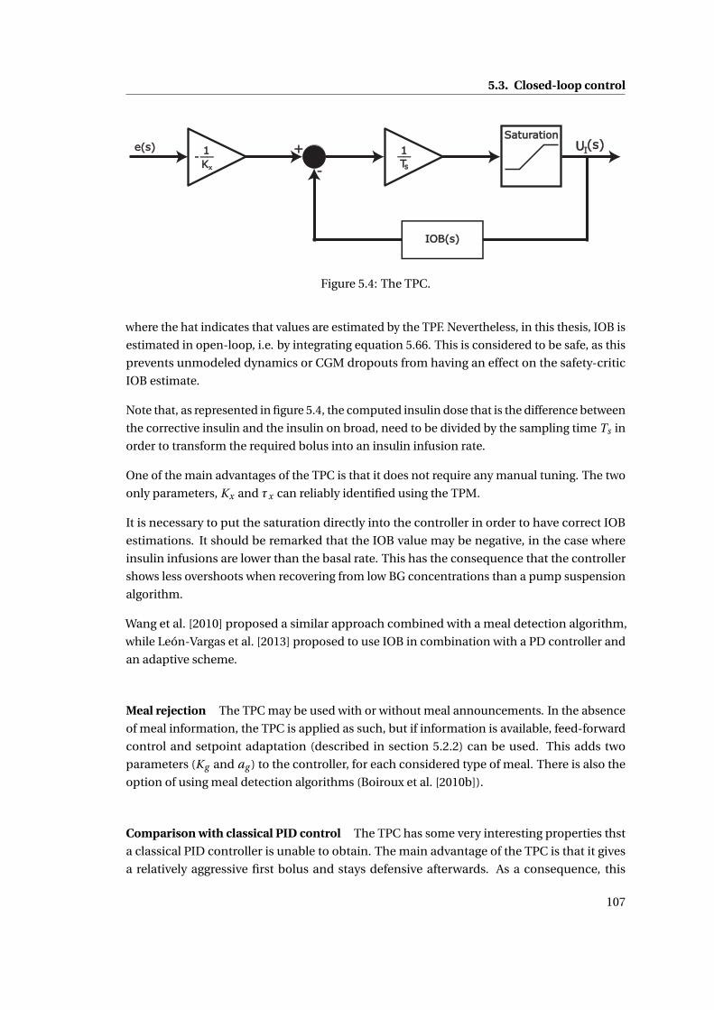
5.3. Closed-loop control
Figure 5.4: The TPC.
where the hat indicates that values are estimated by the TPF. Nevertheless, in this thesis, IOB is
estimated in open-loop, i.e. by integrating equation 5.66. This is considered to be safe, as this
prevents unmodeled dynamics or CGM dropouts from having an effect on the safety-critic
IOB estimate.
Note that, as represented in figure 5.4, the computed insulin dose that is the difference between
the corrective insulin and the insulin on broad, need to be divided by the sampling time Ts in
order to transform the required bolus into an insulin infusion rate.
One of the main advantages of the TPC is that it does not require any manual tuning. The two
only parameters, Kx and τx can reliably identified using the TPM.
It is necessary to put the saturation directly into the controller in order to have correct IOB
estimations. It should be remarked that the IOB value may be negative, in the case where
insulin infusions are lower than the basal rate. This has the consequence that the controller
shows less overshoots when recovering from low BG concentrations than a pump suspension
algorithm.
Wang et al. [2010] proposed a similar approach combined with a meal detection algorithm,
while León-Vargas et al. [2013] proposed to use IOB in combination with a PD controller and
an adaptive scheme.
Meal rejection The TPC may be used with or without meal announcements. In the absence
of meal information, the TPC is applied as such, but if information is available, feed-forward
control and setpoint adaptation (described in section 5.2.2) can be used. This adds two
parameters (Kg and ag ) to the controller, for each considered type of meal. There is also the
option of using meal detection algorithms (Boiroux et al. [2010b]).
Comparison with classical PID control The TPC has some very interesting properties thst
a classical PID controller is unable to obtain. The main advantage of the TPC is that it gives
a relatively aggressive first bolus and stays defensive afterwards. As a consequence, this
107
Chapter 5. BG Control
controller is perfectly suited for rejecting unannounced meals with relatively small reaction
times. The PID, on the other hand, needs to be tuned robustly, because it is prone to large
oscillations otherwise. As a consequence, PID controllers always react slowly to perturbations
such as meals, and, thus, performance is considerably reduced.
However, as there is always a compromise between performance and robustness, the TPC
also has some disadvantages. The TPC manages the rejection of real perturbations very well,
but is sensitive to sensor noise. This means that, if a CGM is used, there is a risk that the
controller gives too much insulin if there is a short spike in CGM readings. This is mostly
benign except when the patient already has a relatively low BG concentration. However,
the impact of this drawback may be reduced using good CGM filters and possibly two CGM
devices simultaneously, as it has been proposed in recent studies (Kovatchev et al. [2013], for
example).
If the TPC is still too aggressive, several measures can be taken:
• Kx can be increased.
• τx can be increased.
• The lower 95% confidence estimate of the BG concentration can be used instead of the
estimated average BG.
5.3.3 Evaluation using the UVa simulator
Implementation
The implementation of the TPC is the same as for the TPC OL given in 5.2.4, with the exception
that it is generally sampled with Ts = 5 minutes and uses CGM measurements. The analyzed
scenario is described in E.1 and is used as a nominal scenario on which all available controllers
are evaluated and compared.
The sampling time was chosen, because this is the most used value in control-related pub-
lished works. However, considering the dominant time constant, this choice might not be the
best: because CGM measurements are noisy with frequencies higher than the glucoregulatory
system cutoff frequency, measurement noise is not filtered and leads to a noisy input signal.
In control theory, the sampling frequency ωs is chosen such that 10ω0 < ωs < 20ω0, where
ω0 is the closed-loop system’s cutoff frequency (Longchamp [2010]). When considering the
sampling period Ts this can be written as τC L3.2 < Ts < τC L
1.6 , where τC L is the closed-loop time
constant. τC L is expected to be close to, or larger, than the TPM’s fastest time constant, i.e. the
minimum of τx and τg . According to table 5.1, this should be around 20 minutes on clinical
study parameters and, according to table 5.3, around 15 minutes on the UVa simulator. These
values may need to be adapted for each patient.
To compare the different controllers, the BGRI (defined in appendix B.4) and the percentage
108
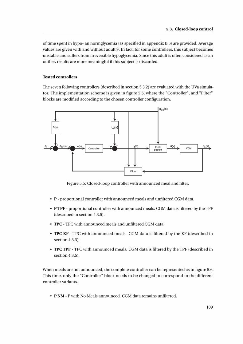
5.3. Closed-loop control
of time spent in hypo- an normglycemia (as specified in appendix B.6) are provided. Average
values are given with and without adult 9. In fact, for some controllers, this subject becomes
unstable and suffers from irreversible hypoglycemia. Since this adult is often considered as an
outlier, results are more meaningful if this subject is discarded.
Tested controllers
The seven following controllers (described in section 5.3.2) are evaluated with the UVa simula-
tor. The implementation scheme is given in figure 5.5, where the "Controller", and "Filter"
blocks are modified according to the chosen controller configuration.
S(s)
Figure 5.5: Closed-loop controller with announced meal and filter.
• P - proportional controller with announced meals and unfiltered CGM data.
• P TPF - proportional controller with announced meals. CGM data is filtered by the TPF
(described in section 4.3.5).
• TPC - TPC with announced meals and unfiltered CGM data.
• TPC KF - TPC with announced meals. CGM data is filtered by the KF (described in
section 4.3.3).
• TPC TPF - TPC with announced meals. CGM data is filtered by the TPF (described in
section 4.3.5).
When meals are not announced, the complete controller can be represented as in figure 5.6.
This time, only the "Controller" block needs to be changed to correspond to the different
controller variants.
• P NM - P with No Meals announced. CGM data remains unfiltered.
109
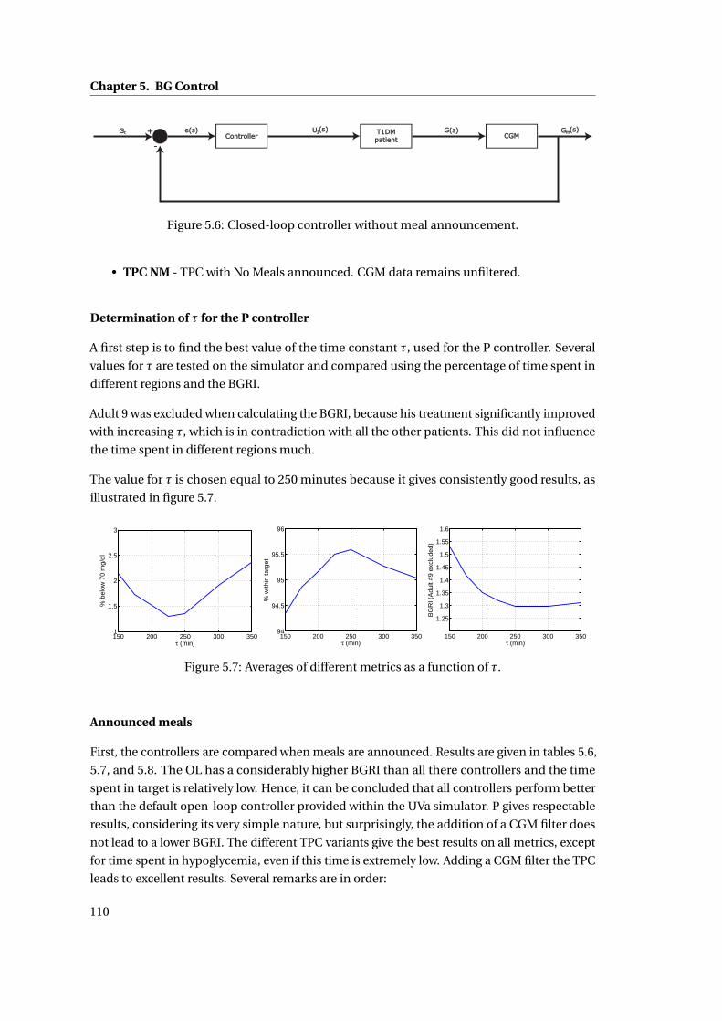
Chapter 5. BG Control
Figure 5.6: Closed-loop controller without meal announcement.
• TPC NM - TPC with No Meals announced. CGM data remains unfiltered.
Determination of τ for the P controller
A first step is to find the best value of the time constant τ, used for the P controller. Several
values for τ are tested on the simulator and compared using the percentage of time spent in
different regions and the BGRI.
Adult 9 was excluded when calculating the BGRI, because his treatment significantly improved
with increasing τ, which is in contradiction with all the other patients. This did not influence
the time spent in different regions much.
The value for τ is chosen equal to 250 minutes because it gives consistently good results, as
illustrated in figure 5.7.
150 200 250 300 3501
1.5
2
2.5
3
τ (min)
% b
elow
70
mg/
dl
150 200 250 300 35094
94.5
95
95.5
96
τ (min)
% w
ithin
targ
et
150 200 250 300 350
1.25
1.3
1.35
1.4
1.45
1.5
1.55
1.6
τ (min)
BG
RI (
Adu
lt #9
exc
lude
d)
Figure 5.7: Averages of different metrics as a function of τ.
Announced meals
First, the controllers are compared when meals are announced. Results are given in tables 5.6,
5.7, and 5.8. The OL has a considerably higher BGRI than all there controllers and the time
spent in target is relatively low. Hence, it can be concluded that all controllers perform better
than the default open-loop controller provided within the UVa simulator. P gives respectable
results, considering its very simple nature, but surprisingly, the addition of a CGM filter does
not lead to a lower BGRI. The different TPC variants give the best results on all metrics, except
for time spent in hypoglycemia, even if this time is extremely low. Adding a CGM filter the TPC
leads to excellent results. Several remarks are in order:
110
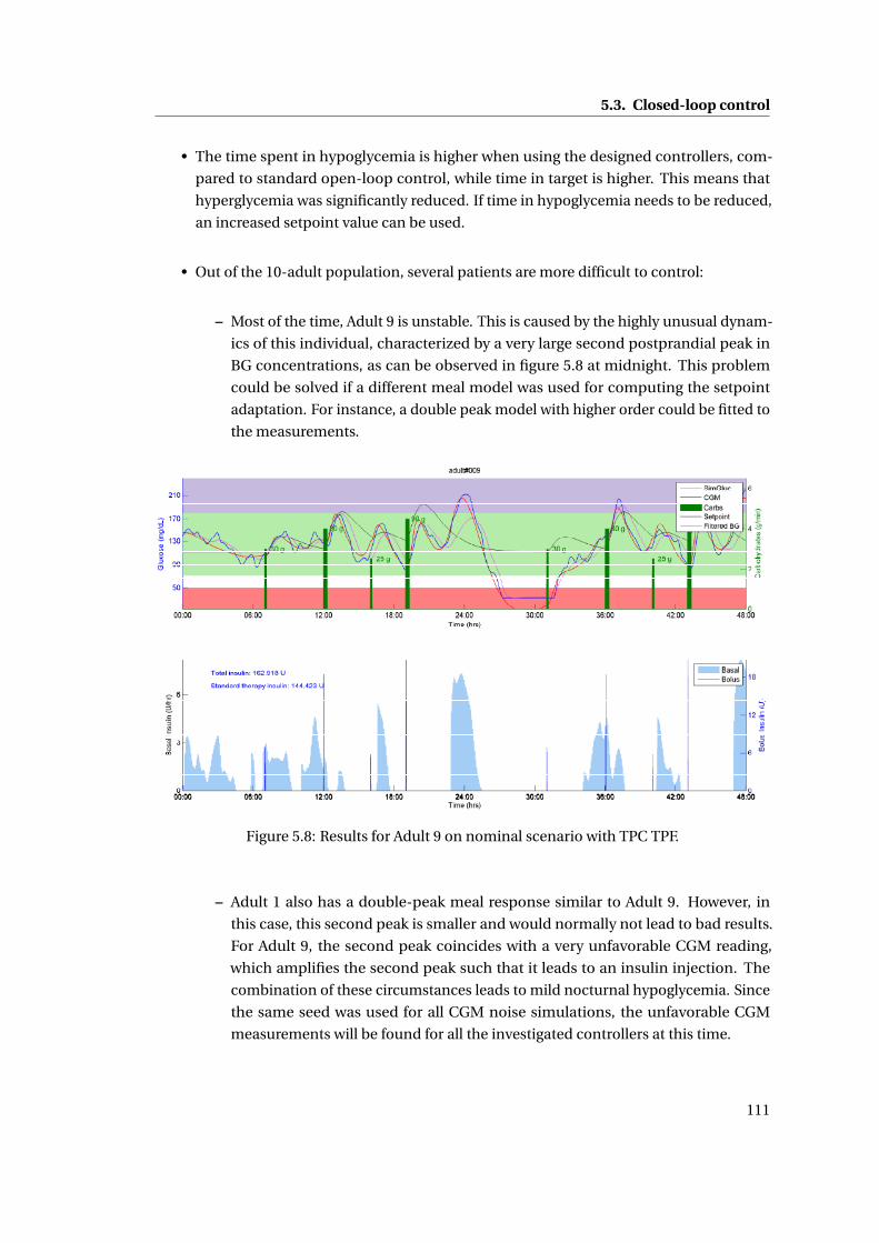
5.3. Closed-loop control
• The time spent in hypoglycemia is higher when using the designed controllers, com-
pared to standard open-loop control, while time in target is higher. This means that
hyperglycemia was significantly reduced. If time in hypoglycemia needs to be reduced,
an increased setpoint value can be used.
• Out of the 10-adult population, several patients are more difficult to control:
– Most of the time, Adult 9 is unstable. This is caused by the highly unusual dynam-
ics of this individual, characterized by a very large second postprandial peak in
BG concentrations, as can be observed in figure 5.8 at midnight. This problem
could be solved if a different meal model was used for computing the setpoint
adaptation. For instance, a double peak model with higher order could be fitted to
the measurements.
Figure 5.8: Results for Adult 9 on nominal scenario with TPC TPF.
– Adult 1 also has a double-peak meal response similar to Adult 9. However, in
this case, this second peak is smaller and would normally not lead to bad results.
For Adult 9, the second peak coincides with a very unfavorable CGM reading,
which amplifies the second peak such that it leads to an insulin injection. The
combination of these circumstances leads to mild nocturnal hypoglycemia. Since
the same seed was used for all CGM noise simulations, the unfavorable CGM
measurements will be found for all the investigated controllers at this time.
111
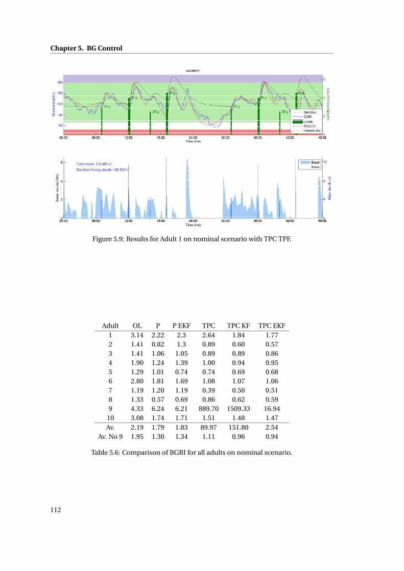
Chapter 5. BG Control
Figure 5.9: Results for Adult 1 on nominal scenario with TPC TPF.
Adult OL P P EKF TPC TPC KF TPC EKF1 3.14 2.22 2.3 2.64 1.84 1.772 1.41 0.82 1.3 0.89 0.60 0.573 1.41 1.06 1.05 0.89 0.89 0.864 1.90 1.24 1.39 1.00 0.94 0.955 1.29 1.01 0.74 0.74 0.69 0.686 2.80 1.81 1.69 1.08 1.07 1.067 1.19 1.20 1.19 0.39 0.50 0.518 1.33 0.57 0.69 0.86 0.62 0.599 4.33 6.24 6.21 889.70 1509.33 16.94
10 3.08 1.74 1.71 1.51 1.48 1.47Av. 2.19 1.79 1.83 89.97 151.80 2.54
Av. No 9 1.95 1.30 1.34 1.11 0.96 0.94
Table 5.6: Comparison of BGRI for all adults on nominal scenario.
112
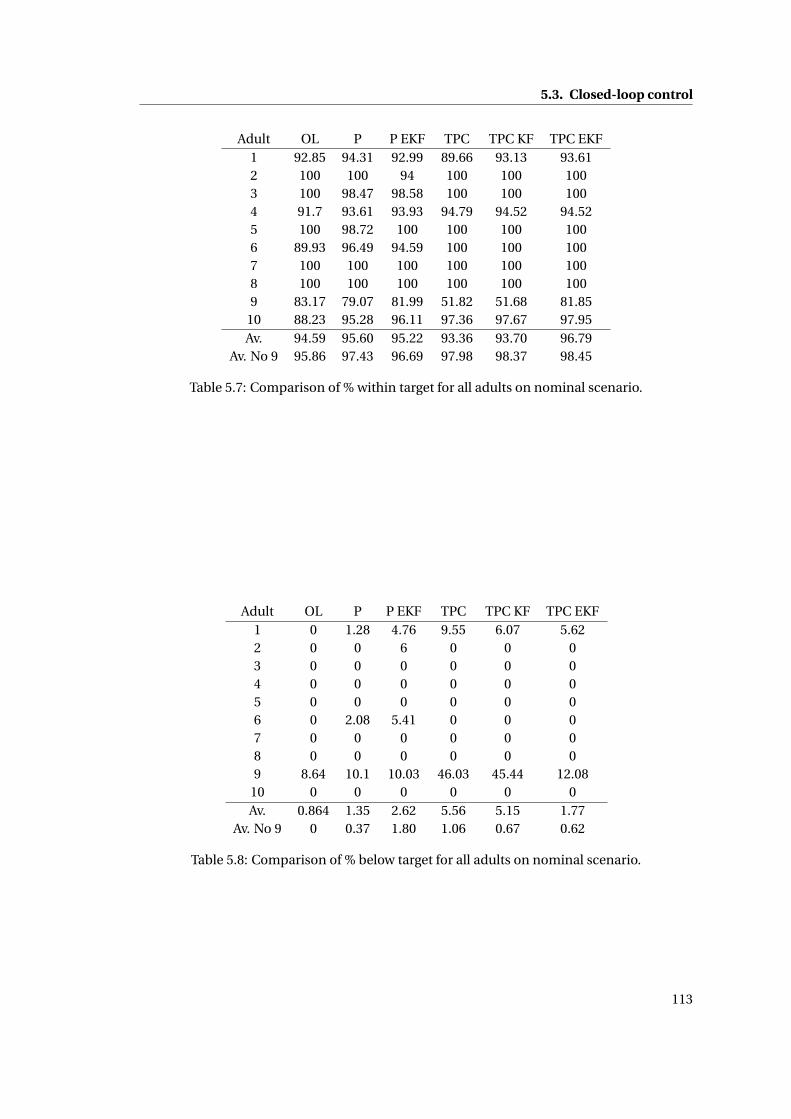
5.3. Closed-loop control
Adult OL P P EKF TPC TPC KF TPC EKF1 92.85 94.31 92.99 89.66 93.13 93.612 100 100 94 100 100 1003 100 98.47 98.58 100 100 1004 91.7 93.61 93.93 94.79 94.52 94.525 100 98.72 100 100 100 1006 89.93 96.49 94.59 100 100 1007 100 100 100 100 100 1008 100 100 100 100 100 1009 83.17 79.07 81.99 51.82 51.68 81.85
10 88.23 95.28 96.11 97.36 97.67 97.95Av. 94.59 95.60 95.22 93.36 93.70 96.79
Av. No 9 95.86 97.43 96.69 97.98 98.37 98.45
Table 5.7: Comparison of % within target for all adults on nominal scenario.
Adult OL P P EKF TPC TPC KF TPC EKF1 0 1.28 4.76 9.55 6.07 5.622 0 0 6 0 0 03 0 0 0 0 0 04 0 0 0 0 0 05 0 0 0 0 0 06 0 2.08 5.41 0 0 07 0 0 0 0 0 08 0 0 0 0 0 09 8.64 10.1 10.03 46.03 45.44 12.08
10 0 0 0 0 0 0Av. 0.864 1.35 2.62 5.56 5.15 1.77
Av. No 9 0 0.37 1.80 1.06 0.67 0.62
Table 5.8: Comparison of % below target for all adults on nominal scenario.
113
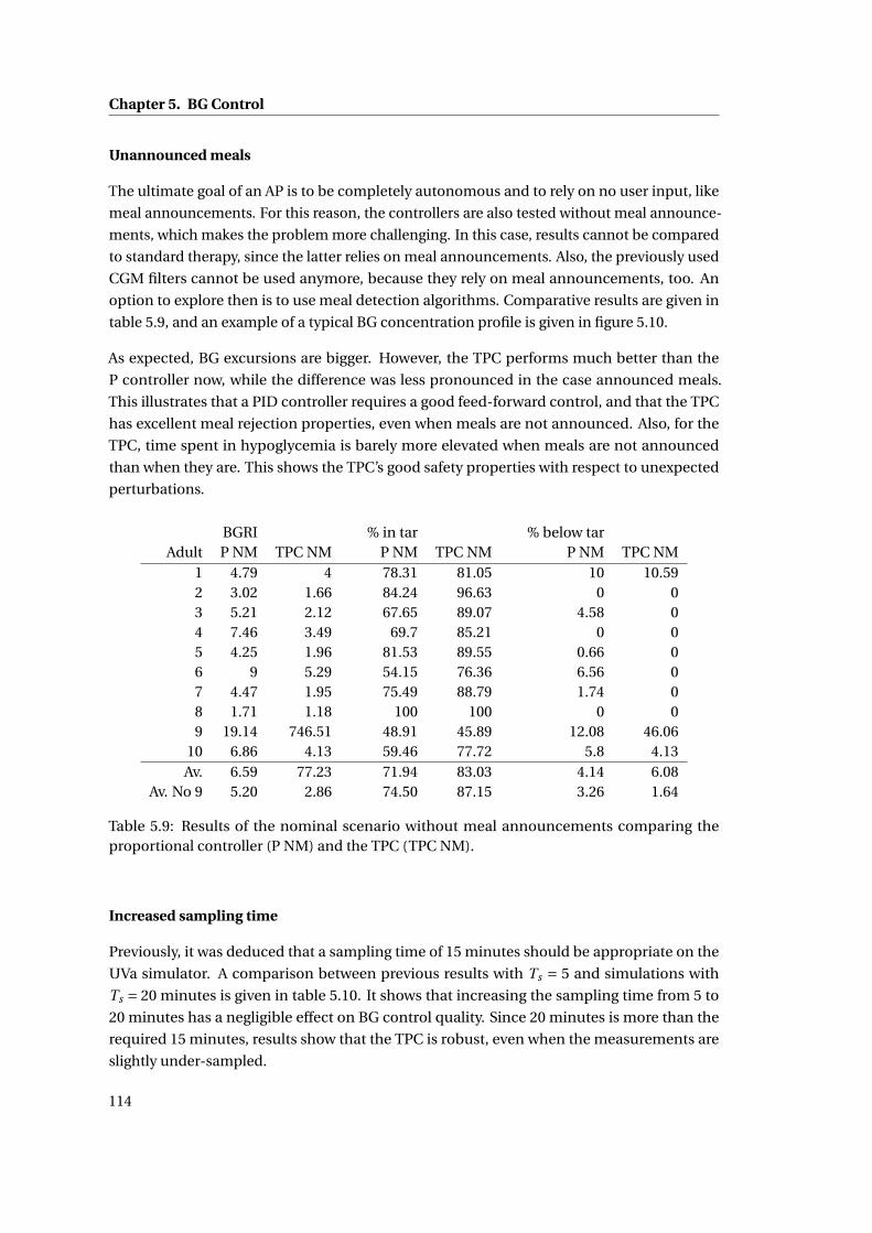
Chapter 5. BG Control
Unannounced meals
The ultimate goal of an AP is to be completely autonomous and to rely on no user input, like
meal announcements. For this reason, the controllers are also tested without meal announce-
ments, which makes the problem more challenging. In this case, results cannot be compared
to standard therapy, since the latter relies on meal announcements. Also, the previously used
CGM filters cannot be used anymore, because they rely on meal announcements, too. An
option to explore then is to use meal detection algorithms. Comparative results are given in
table 5.9, and an example of a typical BG concentration profile is given in figure 5.10.
As expected, BG excursions are bigger. However, the TPC performs much better than the
P controller now, while the difference was less pronounced in the case announced meals.
This illustrates that a PID controller requires a good feed-forward control, and that the TPC
has excellent meal rejection properties, even when meals are not announced. Also, for the
TPC, time spent in hypoglycemia is barely more elevated when meals are not announced
than when they are. This shows the TPC’s good safety properties with respect to unexpected
perturbations.
BGRI % in tar % below tarAdult P NM TPC NM P NM TPC NM P NM TPC NM
1 4.79 4 78.31 81.05 10 10.592 3.02 1.66 84.24 96.63 0 03 5.21 2.12 67.65 89.07 4.58 04 7.46 3.49 69.7 85.21 0 05 4.25 1.96 81.53 89.55 0.66 06 9 5.29 54.15 76.36 6.56 07 4.47 1.95 75.49 88.79 1.74 08 1.71 1.18 100 100 0 09 19.14 746.51 48.91 45.89 12.08 46.06
10 6.86 4.13 59.46 77.72 5.8 4.13Av. 6.59 77.23 71.94 83.03 4.14 6.08
Av. No 9 5.20 2.86 74.50 87.15 3.26 1.64
Table 5.9: Results of the nominal scenario without meal announcements comparing theproportional controller (P NM) and the TPC (TPC NM).
Increased sampling time
Previously, it was deduced that a sampling time of 15 minutes should be appropriate on the
UVa simulator. A comparison between previous results with Ts = 5 and simulations with
Ts = 20 minutes is given in table 5.10. It shows that increasing the sampling time from 5 to
20 minutes has a negligible effect on BG control quality. Since 20 minutes is more than the
required 15 minutes, results show that the TPC is robust, even when the measurements are
slightly under-sampled.
114
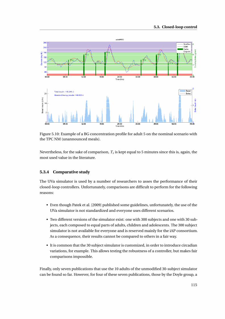
5.3. Closed-loop control
Figure 5.10: Example of a BG concentration profile for adult 5 on the nominal scenario withthe TPC NM (unannounced meals).
Nevertheless, for the sake of comparison, Ts is kept equal to 5 minutes since this is, again, the
most used value in the literature.
5.3.4 Comparative study
The UVa simulator is used by a number of researchers to asses the performance of their
closed-loop controllers. Unfortunately, comparisons are difficult to perform for the following
reasons:
• Even though Patek et al. [2009] published some guidelines, unfortunately, the use of the
UVa simulator is not standardized and everyone uses different scenarios.
• Two different versions of the simulator exist: one with 300 subjects and one with 30 sub-
jects, each composed to equal parts of adults, children and adolescents. The 300 subject
simulator is not available for everyone and is reserved mainly for the iAP consortium.
As a consequence, their results cannot be compared to others in a fair way.
• It is common that the 30 subject simulator is customized, in order to introduce circadian
variations, for example. This allows testing the robustness of a controller, but makes fair
comparisons impossible.
Finally, only seven publications that use the 10 adults of the unmodified 30-subject simulator
can be found so far. However, for four of these seven publications, those by the Doyle group, a
115
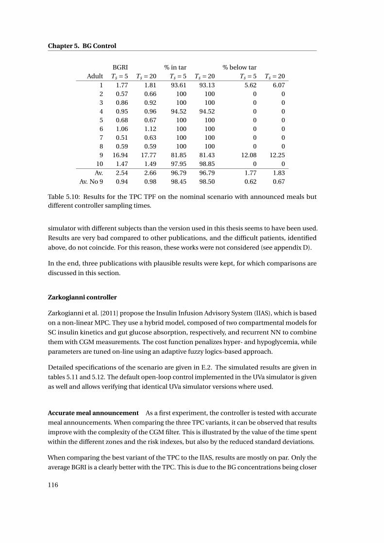
Chapter 5. BG Control
BGRI % in tar % below tarAdult Ts = 5 Ts = 20 Ts = 5 Ts = 20 Ts = 5 Ts = 20
1 1.77 1.81 93.61 93.13 5.62 6.072 0.57 0.66 100 100 0 03 0.86 0.92 100 100 0 04 0.95 0.96 94.52 94.52 0 05 0.68 0.67 100 100 0 06 1.06 1.12 100 100 0 07 0.51 0.63 100 100 0 08 0.59 0.59 100 100 0 09 16.94 17.77 81.85 81.43 12.08 12.25
10 1.47 1.49 97.95 98.85 0 0Av. 2.54 2.66 96.79 96.79 1.77 1.83
Av. No 9 0.94 0.98 98.45 98.50 0.62 0.67
Table 5.10: Results for the TPC TPF on the nominal scenario with announced meals butdifferent controller sampling times.
simulator with different subjects than the version used in this thesis seems to have been used.
Results are very bad compared to other publications, and the difficult patients, identified
above, do not coincide. For this reason, these works were not considered (see appendix D).
In the end, three publications with plausible results were kept, for which comparisons are
discussed in this section.
Zarkogianni controller
Zarkogianni et al. [2011] propose the Insulin Infusion Advisory System (IIAS), which is based
on a non-linear MPC. They use a hybrid model, composed of two compartmental models for
SC insulin kinetics and gut glucose absorption, respectively, and recurrent NN to combine
them with CGM measurements. The cost function penalizes hyper- and hypoglycemia, while
parameters are tuned on-line using an adaptive fuzzy logics-based approach.
Detailed specifications of the scenario are given in E.2. The simulated results are given in
tables 5.11 and 5.12. The default open-loop control implemented in the UVa simulator is given
as well and allows verifying that identical UVa simulator versions where used.
Accurate meal announcement As a first experiment, the controller is tested with accurate
meal announcements. When comparing the three TPC variants, it can be observed that results
improve with the complexity of the CGM filter. This is illustrated by the value of the time spent
within the different zones and the risk indexes, but also by the reduced standard deviations.
When comparing the best variant of the TPC to the IIAS, results are mostly on par. Only the
average BGRI is a clearly better with the TPC. This is due to the BG concentrations being closer
116
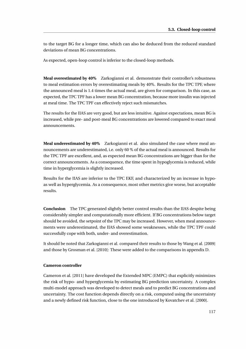
5.3. Closed-loop control
to the target BG for a longer time, which can also be deduced from the reduced standard
deviations of mean BG concentrations.
As expected, open-loop control is inferior to the closed-loop methods.
Meal overestimated by 40% Zarkogianni et al. demonstrate their controller’s robustness
to meal estimation errors by overestimating meals by 40%. Results for the TPC TPF, where
the announced meal is 1.4 times the actual meal, are given for comparison. In this case, as
expected, the TPC TPF has a lower mean BG concentration, because more insulin was injected
at meal time. The TPC TPF can effectively reject such mismatches.
The results for the IIAS are very good, but are less intuitive. Against expectations, mean BG is
increased, while pre- and post-meal BG concentrations are lowered compared to exact meal
announcements.
Meal underestimated by 40% Zarkogianni et al. also simulated the case where meal an-
nouncements are underestimated, i.e. only 60 % of the actual meal is announced. Results for
the TPC TPF are excellent, and, as expected mean BG concentrations are bigger than for the
correct announcements. As a consequence, the time spent in hypoglycemia is reduced, while
time in hyperglycemia is slightly increased.
Results for the IIAS are inferior to the TPC EKF, and characterized by an increase in hypo-
as well as hyperglycemia. As a consequence, most other metrics give worse, but acceptable
results.
Conclusion The TPC generated slightly better control results than the IIAS despite being
considerably simpler and computationally more efficient. If BG concentrations below target
should be avoided, the setpoint of the TPC may be increased. However, when meal announce-
ments were underestimated, the IIAS showed some weaknesses, while the TPC TPF could
successfully cope with both, under- and overestimation.
It should be noted that Zarkogianni et al. compared their results to those by Wang et al. [2009]
and those by Grosman et al. [2010]: These were added to the comparisons in appendix D.
Cameron controller
Cameron et al. [2011] have developed the Extended MPC (EMPC) that explicitly minimizes
the risk of hypo- and hyperglycemia by estimating BG prediction uncertainty. A complex
multi-model approach was developed to detect meals and to predict BG concentrations and
uncertainty. The cost function depends directly on a risk, computed using the uncertainty
and a newly defined risk function, close to the one introduced by Kovatchev et al. [2000].
117
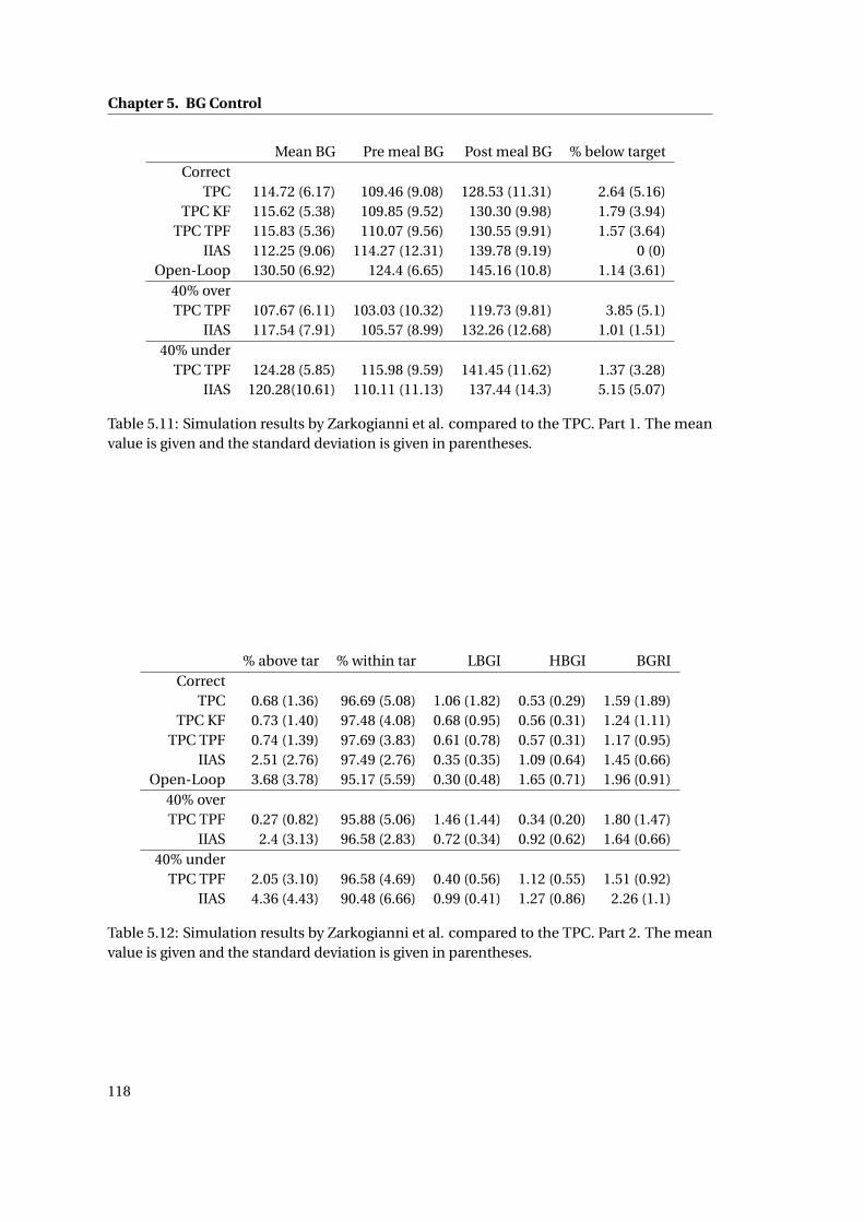
Chapter 5. BG Control
Mean BG Pre meal BG Post meal BG % below targetCorrect
TPC 114.72 (6.17) 109.46 (9.08) 128.53 (11.31) 2.64 (5.16)TPC KF 115.62 (5.38) 109.85 (9.52) 130.30 (9.98) 1.79 (3.94)
TPC TPF 115.83 (5.36) 110.07 (9.56) 130.55 (9.91) 1.57 (3.64)IIAS 112.25 (9.06) 114.27 (12.31) 139.78 (9.19) 0 (0)
Open-Loop 130.50 (6.92) 124.4 (6.65) 145.16 (10.8) 1.14 (3.61)40% overTPC TPF 107.67 (6.11) 103.03 (10.32) 119.73 (9.81) 3.85 (5.1)
IIAS 117.54 (7.91) 105.57 (8.99) 132.26 (12.68) 1.01 (1.51)40% under
TPC TPF 124.28 (5.85) 115.98 (9.59) 141.45 (11.62) 1.37 (3.28)IIAS 120.28(10.61) 110.11 (11.13) 137.44 (14.3) 5.15 (5.07)
Table 5.11: Simulation results by Zarkogianni et al. compared to the TPC. Part 1. The meanvalue is given and the standard deviation is given in parentheses.
% above tar % within tar LBGI HBGI BGRICorrect
TPC 0.68 (1.36) 96.69 (5.08) 1.06 (1.82) 0.53 (0.29) 1.59 (1.89)TPC KF 0.73 (1.40) 97.48 (4.08) 0.68 (0.95) 0.56 (0.31) 1.24 (1.11)
TPC TPF 0.74 (1.39) 97.69 (3.83) 0.61 (0.78) 0.57 (0.31) 1.17 (0.95)IIAS 2.51 (2.76) 97.49 (2.76) 0.35 (0.35) 1.09 (0.64) 1.45 (0.66)
Open-Loop 3.68 (3.78) 95.17 (5.59) 0.30 (0.48) 1.65 (0.71) 1.96 (0.91)40% overTPC TPF 0.27 (0.82) 95.88 (5.06) 1.46 (1.44) 0.34 (0.20) 1.80 (1.47)
IIAS 2.4 (3.13) 96.58 (2.83) 0.72 (0.34) 0.92 (0.62) 1.64 (0.66)40% under
TPC TPF 2.05 (3.10) 96.58 (4.69) 0.40 (0.56) 1.12 (0.55) 1.51 (0.92)IIAS 4.36 (4.43) 90.48 (6.66) 0.99 (0.41) 1.27 (0.86) 2.26 (1.1)
Table 5.12: Simulation results by Zarkogianni et al. compared to the TPC. Part 2. The meanvalue is given and the standard deviation is given in parentheses.
118
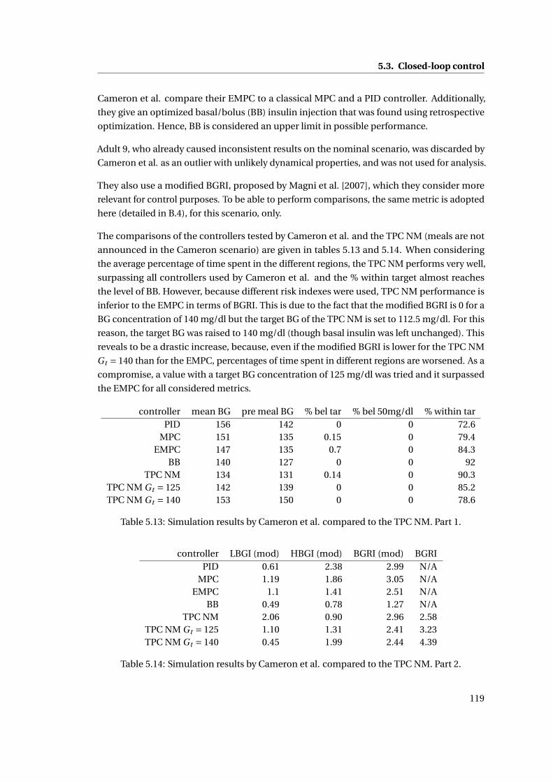
5.3. Closed-loop control
Cameron et al. compare their EMPC to a classical MPC and a PID controller. Additionally,
they give an optimized basal/bolus (BB) insulin injection that was found using retrospective
optimization. Hence, BB is considered an upper limit in possible performance.
Adult 9, who already caused inconsistent results on the nominal scenario, was discarded by
Cameron et al. as an outlier with unlikely dynamical properties, and was not used for analysis.
They also use a modified BGRI, proposed by Magni et al. [2007], which they consider more
relevant for control purposes. To be able to perform comparisons, the same metric is adopted
here (detailed in B.4), for this scenario, only.
The comparisons of the controllers tested by Cameron et al. and the TPC NM (meals are not
announced in the Cameron scenario) are given in tables 5.13 and 5.14. When considering
the average percentage of time spent in the different regions, the TPC NM performs very well,
surpassing all controllers used by Cameron et al. and the % within target almost reaches
the level of BB. However, because different risk indexes were used, TPC NM performance is
inferior to the EMPC in terms of BGRI. This is due to the fact that the modified BGRI is 0 for a
BG concentration of 140 mg/dl but the target BG of the TPC NM is set to 112.5 mg/dl. For this
reason, the target BG was raised to 140 mg/dl (though basal insulin was left unchanged). This
reveals to be a drastic increase, because, even if the modified BGRI is lower for the TPC NM
Gt = 140 than for the EMPC, percentages of time spent in different regions are worsened. As a
compromise, a value with a target BG concentration of 125 mg/dl was tried and it surpassed
the EMPC for all considered metrics.
controller mean BG pre meal BG % bel tar % bel 50mg/dl % within tarPID 156 142 0 0 72.6
MPC 151 135 0.15 0 79.4EMPC 147 135 0.7 0 84.3
BB 140 127 0 0 92TPC NM 134 131 0.14 0 90.3
TPC NM Gt = 125 142 139 0 0 85.2TPC NM Gt = 140 153 150 0 0 78.6
Table 5.13: Simulation results by Cameron et al. compared to the TPC NM. Part 1.
controller LBGI (mod) HBGI (mod) BGRI (mod) BGRIPID 0.61 2.38 2.99 N/A
MPC 1.19 1.86 3.05 N/AEMPC 1.1 1.41 2.51 N/A
BB 0.49 0.78 1.27 N/ATPC NM 2.06 0.90 2.96 2.58
TPC NM Gt = 125 1.10 1.31 2.41 3.23TPC NM Gt = 140 0.45 1.99 2.44 4.39
Table 5.14: Simulation results by Cameron et al. compared to the TPC NM. Part 2.
119
Chapter 5. BG Control
Cormerais controller
Cormerais and Richard [2012] apply EDS to the BMM and validate it on the UVa simulator.
EDS is a nonlinear state feedback method that is based on the idea of imposing certain
dynamic properties to the error. The BMM was identified on UVa simulator-generated training
data. One parameter, the aggressiveness of the controller, needs to be tuned manually, and
additionally, the target BG concentration is manually adjusted to obtain improved results.
All of these values are set using a "trial and error procedure" through different tests on the
simulator that would as well be applicable to a real patient, without endangering him. The
proposed controller does not need any meal announcements. However, it is unclear how all
the necessary state estimations are performed.
Cormerais and Richard use two different scenarios to demonstrate their controller’s abilities:
a 1 day and a 7 day scenario.
1 day scenario This scenario is defined in appendix E.4 and is composed of a single day
with 3 typical meals. Results are in tables 5.15 and 5.16. The TPC NM shows lower averaged
performance for all given metrics. Since the pre-meal BG concentration is about the same
for both controllers, but the post-meal BG concentration is much higher, the main difference
lies within the meal rejection capabilities of both controllers. Considering that meals are
not announced, EDS results are outstanding. In order to obtain comparable post-meal and
maximum BG concentrations, the target BG concentration of the TPC NM was reduced to
100mg/dl. However, in this case, the risk of hypoglycemia increases.
mean BG pre m BG post m BG % bel tar % ab tar % bel 50mg/dlCormerais 126.58 104.21 164.52 0.0 4.3 0.0
TPC NM 130.02 104.67 181.84 0.5 8.7 0.0TPC NM Gt = 100 119.87 94.19 169.52 1.9 6.0 0.0
Table 5.15: Simulation results by Cormerais and Richard compared to the TPC on the 1 dayscenario. Part 1.
% within tar LBGI HBGI BGRI min BG max BGCormerais 95.7 0.11 1.45 1.56 91.1 187.7
TPC NM 90.8 0.24 2.11 2.35 83.1 202.8TPC NM Gt = 100 92.1 0.57 1.43 2.00 74.9 189.6
Table 5.16: Simulation results by Cormerais and Richard compared to the TPC on the 1 dayscenario. Part 2.
7 day scenario This second scenario is designed to show the robustness of EDS with respect
to meal variability. The meal amounts and meal times are randomly modified and meals of up
to 120g of CHO are ingested. This puts an increased strain on the tested controllers and, as
shown in tables 5.17 and 5.18, leads to higher BGRI values. In this case, the different versions
120
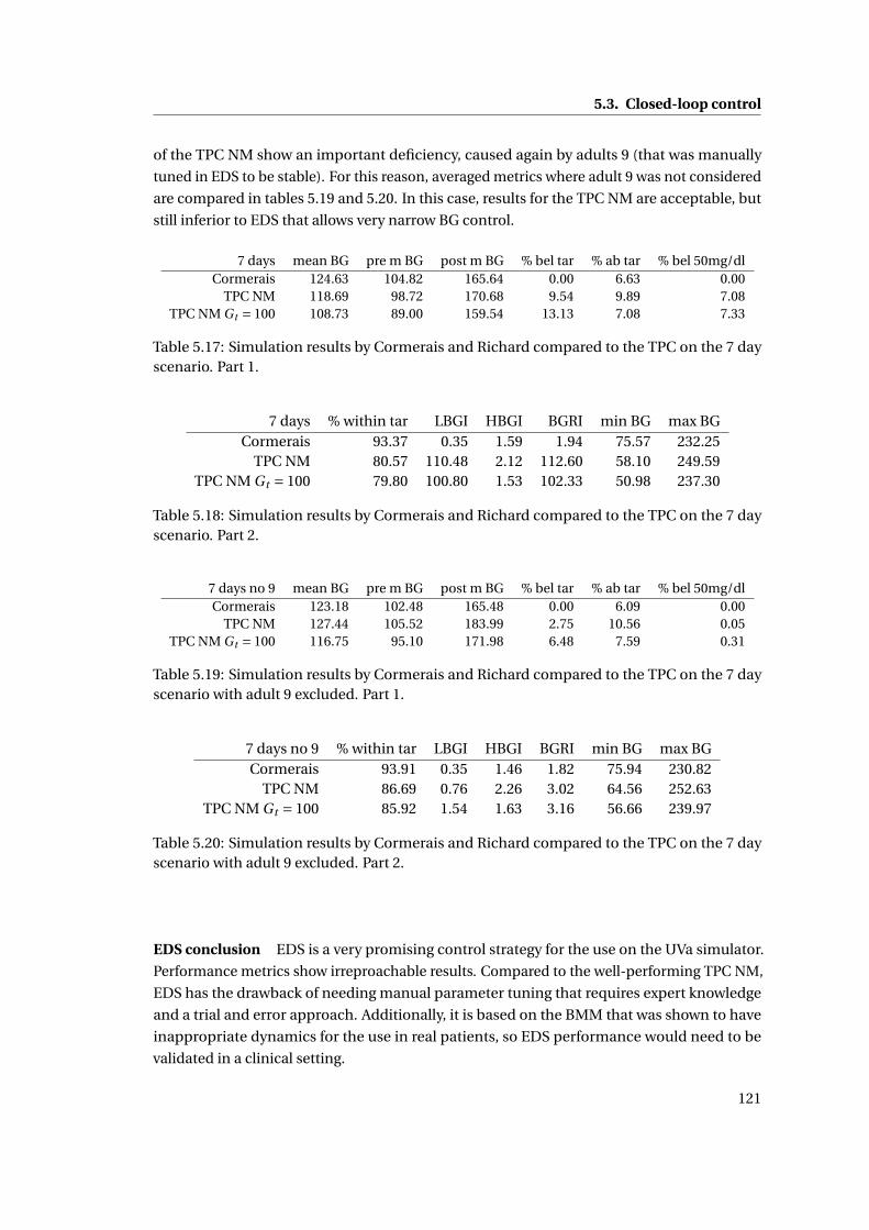
5.3. Closed-loop control
of the TPC NM show an important deficiency, caused again by adults 9 (that was manually
tuned in EDS to be stable). For this reason, averaged metrics where adult 9 was not considered
are compared in tables 5.19 and 5.20. In this case, results for the TPC NM are acceptable, but
still inferior to EDS that allows very narrow BG control.
7 days mean BG pre m BG post m BG % bel tar % ab tar % bel 50mg/dlCormerais 124.63 104.82 165.64 0.00 6.63 0.00
TPC NM 118.69 98.72 170.68 9.54 9.89 7.08TPC NM Gt = 100 108.73 89.00 159.54 13.13 7.08 7.33
Table 5.17: Simulation results by Cormerais and Richard compared to the TPC on the 7 dayscenario. Part 1.
7 days % within tar LBGI HBGI BGRI min BG max BGCormerais 93.37 0.35 1.59 1.94 75.57 232.25
TPC NM 80.57 110.48 2.12 112.60 58.10 249.59TPC NM Gt = 100 79.80 100.80 1.53 102.33 50.98 237.30
Table 5.18: Simulation results by Cormerais and Richard compared to the TPC on the 7 dayscenario. Part 2.
7 days no 9 mean BG pre m BG post m BG % bel tar % ab tar % bel 50mg/dlCormerais 123.18 102.48 165.48 0.00 6.09 0.00
TPC NM 127.44 105.52 183.99 2.75 10.56 0.05TPC NM Gt = 100 116.75 95.10 171.98 6.48 7.59 0.31
Table 5.19: Simulation results by Cormerais and Richard compared to the TPC on the 7 dayscenario with adult 9 excluded. Part 1.
7 days no 9 % within tar LBGI HBGI BGRI min BG max BGCormerais 93.91 0.35 1.46 1.82 75.94 230.82
TPC NM 86.69 0.76 2.26 3.02 64.56 252.63TPC NM Gt = 100 85.92 1.54 1.63 3.16 56.66 239.97
Table 5.20: Simulation results by Cormerais and Richard compared to the TPC on the 7 dayscenario with adult 9 excluded. Part 2.
EDS conclusion EDS is a very promising control strategy for the use on the UVa simulator.
Performance metrics show irreproachable results. Compared to the well-performing TPC NM,
EDS has the drawback of needing manual parameter tuning that requires expert knowledge
and a trial and error approach. Additionally, it is based on the BMM that was shown to have
inappropriate dynamics for the use in real patients, so EDS performance would need to be
validated in a clinical setting.
121
Chapter 5. BG Control
5.4 Outlook on sTPM-based BG control
The TPC, based on the deterministic TPM, shows promising results on the UVa simulator, but
several sTPM-based control methods and applications have the potential to improve diabetes
treatment even further. These approaches are shortly introduced, but not covered in detail in
this thesis.
5.4.1 Pump suspension
The sTPM introduces the possibility to monitor the uncertainty of the BG concentration on
top of simple BG predictions. This can be put to good use in the context of pump suspension
algorithms. The recently FDA-approved algorithm by Medtronic [2013], for example, suspends
the insulin pump if the BG concentration passes a predefined threshold. Because of the
important delays in the system (cf. 1.2.6) this preventive action may occur too late and
hypoglycemia may occur, even tough to a lesser extend. Model predictions could thus be
used to predict and avoid future hypoglycemia by acting before its occurrence (Cameron
et al. [2012]). The sTPM allows adding an additional layer to such a suspension algorithm by
predicting the risk of hypoglycemia, instead of the simple prediction of the most likely BG
concentration. The TPF would be an ideal candidate to give such predictions, although the
algorithm that defines the needed actions still has to be developed.
5.4.2 Open-loop optimal control using sTPM
In section 5.2, the optimal feed-forward control for meal disturbance rejection has been
designed. However, if the additional uncertainty information provided by the sTPM was
taken into account, the optimal feed-forward control would change, depending on the chosen
cost function. To solve this problem, an optimization would need to run after each SMBG
measurement in order to compute the optimal insulin infusion (Prud’homme et al. [2011]).
For example, good results would be expected by minimizing the cost function JsT P M on a
control and prediction horizon hc :
JsT P M (UI ) =Nc∑
k=0(kov(G(k,UI ))+kov(G(k,UI ))), (5.72)
where Nc is the number of samples within hc , kov is the Kovatchev risk function given in
appendix B.4, G is the estimated upper 95% confidence limit, G is the estimated lower 95 %
confidence limit, and UI is the insulin infusion profile. This cost function would ensure that
the patient’s risk is minimal. If uncertainty would be zero, the method would impose a target
BG of 112.5 mg/dl, while this value would increase with uncertainty.
122

5.5. Conclusion
5.4.3 MPC using sTPM
Just like the TPC is a regularly sampled version of the TPC OL, an MPC is a regularly sam-
pled version of open-loop optimal control. This means that the open-loop optimal control
method using the sTPM, described in the previous paragraph, can be generalized to give an
MPC based on the sTPM. This stochastic Therapy Parameter-based Controller (sTPC) would
explicitly minimize the patient risk in a similar way as Cameron et al. [2011] and improve
safety, compared with the TPC.
5.4.4 SMBG measurement reminder
The sTPM provides a quality evaluation for BG predictions. This property can be used for a
SMBG measurement reminder. If the confidence in predictions gets too low, the patient could
be asked to take a SMBG measurement. A drawback of such a method is that, if a patient’s
parameters are prone to be relatively uncertain, these reminders may be given at a high
frequency, which may be annoying for the patient. However these frequent measurements
could be used to update the model parameters, thus reducing the number of future reminders.
This idea can be extended using CGM measurements: the TPF can be run to update uncer-
tainties and, when CGM measurements start falling outside the confidence region, a new
calibration SMBG measurement can be requested.
5.4.5 Meal and fault detection
A CGM device, in combination with the TPF, can be used for detecting unexpected BG mea-
surements. If stochastic model predictions do not coincide with the CGM measurements
anymore, the patient may, for example, have taken a meal, have been doing some exercise, or
have a problem with his insulin pump, or CGM device. Detecting unannounced meals, and
reminding patients to announce them, may lead to improved BG control as suggested by the
results of section 5.3.3.
5.5 Conclusion
The new TPM equations were used to construct an optimal open-loop control strategy that
allows keeping BG concentrations as close to the target BG as possible. The resulting TPC OL
adds three features to conventional standard therapy:
• Feed-forward for meal disturbance rejection.
• Setpoint adaptation in case a meal disturbance cannot fully be rejected.
• Improved insulin correction using TPM-based IOB.
123
Chapter 5. BG Control
The open-loop control strategy was then extended to construct a closed-loop controller,
referred to as the TPC, which applies TPC OL at each CGM sampling time. Additionally, the
TPF was used to filter CGM measurements and improve BG estimation. This AP is a very
simple and effective method that requires minimal computational resources. The tuning
of these controllers can be fully automatized and no manual tuning is necessary. However,
manual tuning is still possible, because only two intuitive parameters need to be set in the
TPC NM, while two more for every additional type of meal to be announced.
The open challenges defined in the state of the art (5.3.1) are addressed by the new controllers:
the combination of the methods introduced in the TPC OL and TPC is designed such that
hyperglycemia is rejected as fast as possible while always avoiding BG concentrations lower
than the setpoint. Hence the asymmetric control objective is considered directly in the
controller’s structure. As a consequence, BG concentrations that are lower than the setpoint
should never occur and negative insulin infusions should never be required, if the TPM is
accurate. Nevertheless, if this happens, because of unmodeled effects, required negative
insulin infusions will be small and can be applied by reducing the basal rate. Using this
mechanism, the negative effect of the control saturation is reduced to a minimum. Finally,
the time delay of the effect of insulin infusions on the BG concentration is taken into account
through the time constant of the IOB.
The new controllers were evaluated on the UVa simulator, showing that
• Standard therapy, which is successfully used for real patients, shows bad performance
on the UVa simulator, revealing one of the limits of the simulator. TPC OL probably does
not lead to much better results.
• The TPC gives excellent results on the UVa simulator with both announced and unan-
nounced meals, reducing patient risk (lower BGRI) and improves treatment quality
(increased % of time in target range). These results are confirmed by a comparison
with other published controllers that are considerably more complex, but show slightly
inferior results, with the exception of EDS that shows better results.
Several remarks are in order:
• The TPC OL and TPC are based on the TPM and are the best possible solutions with
this model. However, since it is not accurate, resulting control will not be perfect, either.
However, since the TPM is the model showing best prediction capabilities (cf. chapter
2), the derived controllers perform quite well.
• Controller testing is only done on the UVa simulator. While this gives first insight into a
controller’s behavior, it is not a reliable measure of controller performance. The results
are only valid within the UVa simulator framework, but will be different for real patients.
This is especially true for TPM-based controllers, as there is a significant mismatch
124
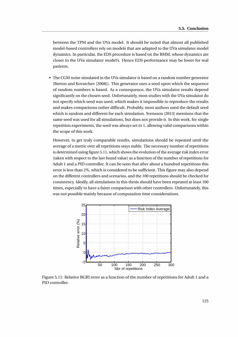
5.5. Conclusion
between the TPM and the UVa model. It should be noted that almost all published
model-based controllers rely on models that are adapted to the UVa simulator model
dynamics. In particular, the EDS procedure is based on the BMM, whose dynamics are
closer to the UVa simulator model’s. Hence EDS performance may be lower for real
patients.
• The CGM noise simulated in the UVa simulator is based on a random number generator
(Breton and Kovatchev [2008]). This generator uses a seed upon which the sequence
of random numbers is based. As a consequence, the UVa simulator results depend
significantly on the chosen seed. Unfortunately, most studies with the UVa simulator do
not specify which seed was used, which makes it impossible to reproduce the results
and makes comparisons rather difficult. Probably, most authors used the default seed
which is random and different for each simulation. Svensson [2013] mentions that the
same seed was used for all simulations, but does not provide it. In this work, for single
repetition experiments, the seed was always set to 1, allowing valid comparisons within
the scope of this work.
However, to get truly comparable results, simulations should be repeated until the
average of a metric over all repetitions stays stable. The necessary number of repetitions
is determined using figure 5.11, which shows the evolution of the average risk index error
(taken with respect to the last found value) as a function of the number of repetitions for
Adult 1 and a PID controller. It can be seen that after about a hundred repetitions this
error is less than 2%, which is considered to be sufficient. This figure may also depend
on the different controllers and scenarios, and the 100 repetitions should be checked for
consistency. Ideally, all simulations in this thesis should have been repeated at least 100
times, especially to have a fairer comparison with other controllers. Unfortunately, this
was not possible mainly because of computation time considerations.
50 100 150 200 250 300−5
0
5
10
15
20
25
Nbr of repetitions
Rel
ativ
e er
ror
(%)
Risk Index Average
Figure 5.11: Relative BGRI error as a function of the number of repetitions for Adult 1 and aPID controller.
125

Chapter 5. BG Control
• The proposed control algorithms are relatively safe since they are directly inspired by
standard therapy (considered as safe), but have additional safety measures such as the
IOB and the adapted setpoint. Nevertheless, safety cannot always be guaranteed and,
for unfortunate circumstances or, in case of unexpected BG dynamics, excessive insulin
doses may be administered. The example of adult 9 illustrates this danger, even though
his meal response appears to be exceptional. A sTPM-based control algorithm may be
able to supply this final security layer.
126
6 Conclusion
6.1 Summary
This thesis proposes an AP that tackles most important challenges of BG control (section 1.2) by
using standard therapy, a reliable and widely used treatment method. The therapy parameters
are explicitly introduced into the proposed method in order to create a well-accepted, intuitive,
and reliable treatment option.
Several components, sharing the concept of therapy parameters, were developed and com-
bined to create a complete treatment approach: the AP is fully specified and does not need
any additional, manual tuning. The only requirement is an appropriate data set to identify the
model parameters. The components are the following:
• Prediction models (TPM and TPM+) directly based on therapy parameters.
• BG estimator for filtering CGM measurements (TPF) based on the prediction models.
• Open- and closed-loop control algorithm (TPC) based on the prediction models.
These components address several of the above-mentioned challenges, as illustrated in table
6.1. The uncertainty is split into different categories that are separately addressed by some of
the proposed components: Inter-patient variability is considered by identifying parameters for
every individual instead of using population parameters. Hence, the therapy is individualized
and differences between patients have no influence on their therapy. Intra-patient variability
is not taken into account in the proposed controller, yet, measurement noise is being filtered
out using the TPC. Meal announcement errors are not taken into account directly, either.
However, it was shown that the TPC has good performance, even if meals are not announced
at all, making the TPC robust against meal announcement errors. Meal uptake variability is
considered by identifying new model parameters for every type of meal, and, indirectly, by the
meal rejection properties of the TPC. This is done analogously to the individual identification
for the different patients, but cannot be demonstrated in this thesis, because the necessary
127
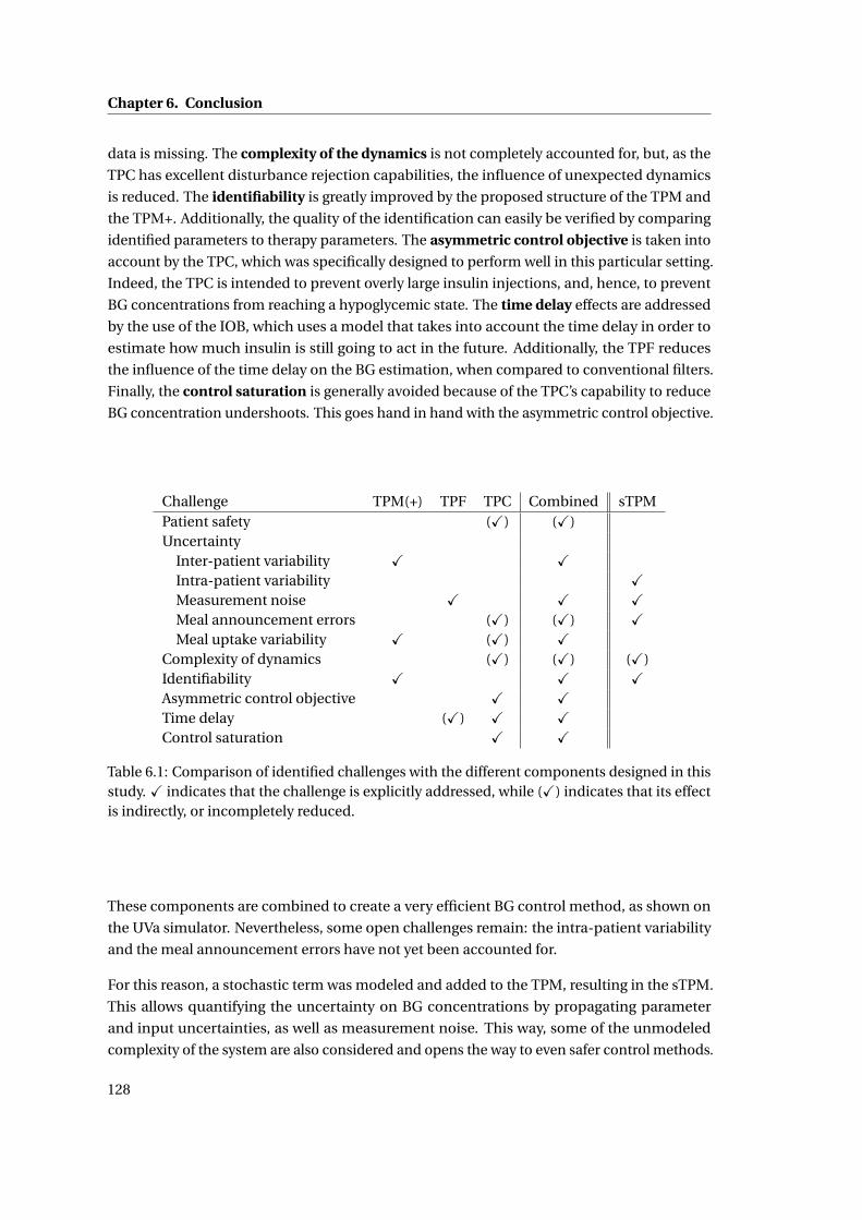
Chapter 6. Conclusion
data is missing. The complexity of the dynamics is not completely accounted for, but, as the
TPC has excellent disturbance rejection capabilities, the influence of unexpected dynamics
is reduced. The identifiability is greatly improved by the proposed structure of the TPM and
the TPM+. Additionally, the quality of the identification can easily be verified by comparing
identified parameters to therapy parameters. The asymmetric control objective is taken into
account by the TPC, which was specifically designed to perform well in this particular setting.
Indeed, the TPC is intended to prevent overly large insulin injections, and, hence, to prevent
BG concentrations from reaching a hypoglycemic state. The time delay effects are addressed
by the use of the IOB, which uses a model that takes into account the time delay in order to
estimate how much insulin is still going to act in the future. Additionally, the TPF reduces
the influence of the time delay on the BG estimation, when compared to conventional filters.
Finally, the control saturation is generally avoided because of the TPC’s capability to reduce
BG concentration undershoots. This goes hand in hand with the asymmetric control objective.
Challenge TPM(+) TPF TPC Combined sTPMPatient safety (X) (X)Uncertainty
Inter-patient variability X XIntra-patient variability XMeasurement noise X X XMeal announcement errors (X) (X) XMeal uptake variability X (X) X
Complexity of dynamics (X) (X) (X)Identifiability X X XAsymmetric control objective X XTime delay (X) X XControl saturation X X
Table 6.1: Comparison of identified challenges with the different components designed in thisstudy. X indicates that the challenge is explicitly addressed, while (X) indicates that its effectis indirectly, or incompletely reduced.
These components are combined to create a very efficient BG control method, as shown on
the UVa simulator. Nevertheless, some open challenges remain: the intra-patient variability
and the meal announcement errors have not yet been accounted for.
For this reason, a stochastic term was modeled and added to the TPM, resulting in the sTPM.
This allows quantifying the uncertainty on BG concentrations by propagating parameter
and input uncertainties, as well as measurement noise. This way, some of the unmodeled
complexity of the system are also considered and opens the way to even safer control methods.
128
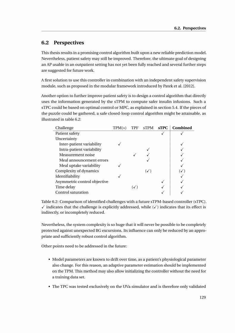
6.2. Perspectives
6.2 Perspectives
This thesis results in a promising control algorithm built upon a new reliable prediction model.
Nevertheless, patient safety may still be improved. Therefore, the ultimate goal of designing
an AP usable in an outpatient setting has not yet been fully reached and several further steps
are suggested for future work.
A first solution to use this controller in combination with an independent safety supervision
module, such as proposed in the modular framework introduced by Patek et al. [2012].
Another option to further improve patient safety is to design a control algorithm that directly
uses the information generated by the sTPM to compute safer insulin infusions. Such a
sTPC could be based on optimal control or MPC, as explained in section 5.4. If the pieces of
the puzzle could be gathered, a safe closed-loop control algorithm might be attainable, as
illustrated in table 6.2:
Challenge TPM(+) TPF sTPM sTPC CombinedPatient safety X XUncertainty
Inter-patient variability X XIntra-patient variability X XMeasurement noise X X XMeal announcement errors X XMeal uptake variability X X
Complexity of dynamics (X) (X)Identifiability X XAsymmetric control objective X XTime delay (X) X XControl saturation X X
Table 6.2: Comparison of identified challenges with a future sTPM-based controller (sTPC).X indicates that the challenge is explicitly addressed, while (X) indicates that its effect isindirectly, or incompletely reduced.
Nevertheless, the system complexity is so huge that it will never be possible to be completely
protected against unexpected BG excursions. Its influence can only be reduced by an appro-
priate and sufficiently robust control algorithm.
Other points need to be addressed in the future:
• Model parameters are known to drift over time, as a patient’s physiological parameter
also change. For this reason, an adaptive parameter estimation should be implemented
on the TPM. This method may also allow initializing the controller without the need for
a training data set.
• The TPC was tested exclusively on the UVa simulator and is therefore only validated
129
Chapter 6. Conclusion
in the light of the known limitations of this simulator. In order to truly validate the
proposed algorithms, they would need to be tested on real patients. It should be noted
that the TPM was designed on real patient data and not on UVa simulations. As a
consequence, the potential of the TPM and of related control methods is certainly
higher on real data.
• The effect of exercise is one of the external disturbances with a significant effect on BG
concentrations and whose cause may be measured. For this reason, an exercise model
that follows the design methods of the TPM should be designed.
• The proposed models and controllers should not only be tested on the adult population
of the UVa simulator, but also on the children and adolescents. Good results would
indicate good robustness of the proposed methods, because these patients are more
difficult to control, because of their increased insulin sensitivity and variability.
130
A Validation data
A.1 UVa/Padova simulator
The FDA-approved in silico testing of diabetes control strategies in order to replace pre-clinical
animal testing. The approved software is called the UVa/Padova simulator (referred to as the
UVa simulator in this thesis) and is based on a high-order model by Dalla Man et al. Dalla
Man et al. [2007]. This simulator, also known as the Type 1 Diabetes Metabolic Simulator, is
currently the most important benchmark for control strategy evaluation, and it is important
for proposed methods to perform well on generated simulator data.
The UVa simulator exists in two versions: a 300- and a 30-subject version. The larger version is
reserved for selected research groups only, while the smaller version is used in this work. Out
of the 30 available subjects, there are 10 adults, 10 children, and 10 adolescents. Only the 10
adults are considered here for the following reasons: (i) It is computationally more efficient to
do the first tests on less subjects, (ii) children and adolescents are more difficult to control and
the simplest case should be analyzed first, and (iii) most published controllers were validated
on adult data only (as for the ones compared in section 5.3.4).
The UVa simulator allows interactions with the virtual subject population by setting an insulin
injection rate (the insulin profile can be adapted at a sampling time of 1 minute and at incre-
ments of 0.05 U/h) or by determining the CHO intake rate. Only a single type of mixed meal is
available. The provided outputs are BG concentrations, both exact and CGM measurements.
An example of such an output is given in figure A.1. The CGM measurements are based on a
model by Breton and Kovatchev [2008] that uses the exact values to generate the noisy ones
colored noise and a stochastic process. This stochastic process is simulated based on the
initial seed of a random number generator. In this thesis, this seed was always chosen equal to
1.
The dynamics of the underlying model are non-linear and relatively complex. Nevertheless,
insulin and meal sensitivities only change to limited degree over the BG concentration range.
For this reason, the developers are able to provide values for CF and I2C that are appropriate.
131
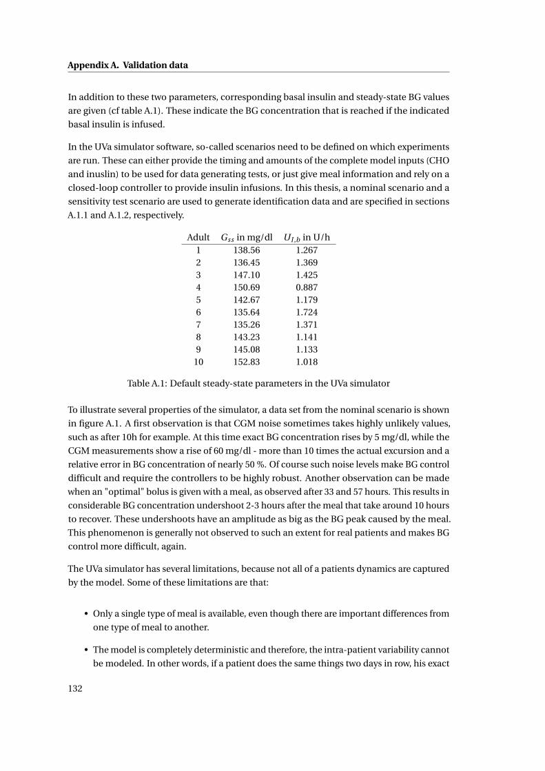
Appendix A. Validation data
In addition to these two parameters, corresponding basal insulin and steady-state BG values
are given (cf table A.1). These indicate the BG concentration that is reached if the indicated
basal insulin is infused.
In the UVa simulator software, so-called scenarios need to be defined on which experiments
are run. These can either provide the timing and amounts of the complete model inputs (CHO
and inuslin) to be used for data generating tests, or just give meal information and rely on a
closed-loop controller to provide insulin infusions. In this thesis, a nominal scenario and a
sensitivity test scenario are used to generate identification data and are specified in sections
A.1.1 and A.1.2, respectively.
Adult Gss in mg/dl UI ,b in U/h1 138.56 1.2672 136.45 1.3693 147.10 1.4254 150.69 0.8875 142.67 1.1796 135.64 1.7247 135.26 1.3718 143.23 1.1419 145.08 1.133
10 152.83 1.018
Table A.1: Default steady-state parameters in the UVa simulator
To illustrate several properties of the simulator, a data set from the nominal scenario is shown
in figure A.1. A first observation is that CGM noise sometimes takes highly unlikely values,
such as after 10h for example. At this time exact BG concentration rises by 5 mg/dl, while the
CGM measurements show a rise of 60 mg/dl - more than 10 times the actual excursion and a
relative error in BG concentration of nearly 50 %. Of course such noise levels make BG control
difficult and require the controllers to be highly robust. Another observation can be made
when an "optimal" bolus is given with a meal, as observed after 33 and 57 hours. This results in
considerable BG concentration undershoot 2-3 hours after the meal that take around 10 hours
to recover. These undershoots have an amplitude as big as the BG peak caused by the meal.
This phenomenon is generally not observed to such an extent for real patients and makes BG
control more difficult, again.
The UVa simulator has several limitations, because not all of a patients dynamics are captured
by the model. Some of these limitations are that:
• Only a single type of meal is available, even though there are important differences from
one type of meal to another.
• The model is completely deterministic and therefore, the intra-patient variability cannot
be modeled. In other words, if a patient does the same things two days in row, his exact
132
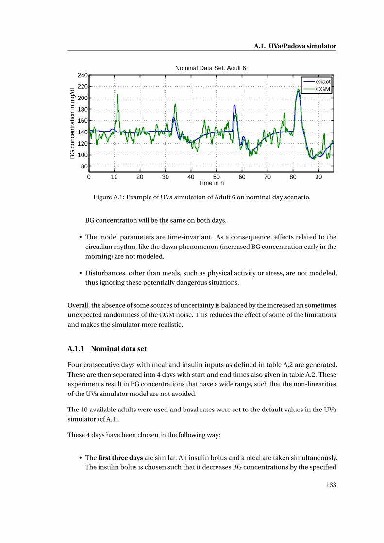
A.1. UVa/Padova simulator
0 10 20 30 40 50 60 70 80 90
80
100
120
140
160
180
200
220
240
Time in h
BG
con
cent
ratio
n in
mg/
dlNominal Data Set. Adult 6.
exactCGM
Figure A.1: Example of UVa simulation of Adult 6 on nominal day scenario.
BG concentration will be the same on both days.
• The model parameters are time-invariant. As a consequence, effects related to the
circadian rhythm, like the dawn phenomenon (increased BG concentration early in the
morning) are not modeled.
• Disturbances, other than meals, such as physical activity or stress, are not modeled,
thus ignoring these potentially dangerous situations.
Overall, the absence of some sources of uncertainty is balanced by the increased an sometimes
unexpected randomness of the CGM noise. This reduces the effect of some of the limitations
and makes the simulator more realistic.
A.1.1 Nominal data set
Four consecutive days with meal and insulin inputs as defined in table A.2 are generated.
These are then seperated into 4 days with start and end times also given in table A.2. These
experiments result in BG concentrations that have a wide range, such that the non-linearities
of the UVa simulator model are not avoided.
The 10 available adults were used and basal rates were set to the default values in the UVa
simulator (cf A.1).
These 4 days have been chosen in the following way:
• The first three days are similar. An insulin bolus and a meal are taken simultaneously.
The insulin bolus is chosen such that it decreases BG concentrations by the specified
133
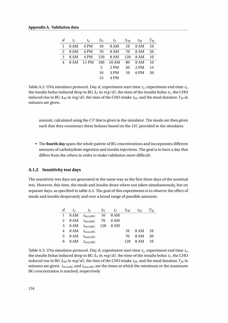
Appendix A. Validation data
d ts te ∆I tI ∆M tM TM
1 8 AM 4 PM 10 8 AM 10 8 AM 102 8 AM 4 PM 70 8 AM 70 8 AM 203 8 AM 4 PM 120 8 AM 120 8 AM 104 8 AM 11 PM 100 10 AM 80 8 AM 10
5 2 PM 20 2 PM 1510 3 PM 10 6 PM 2015 4 PM
Table A.2: UVa simulator protocol. Day d , experiment start time ts , experiment end time te ,the insulin bolus induced drop in BG ∆I in mg /dl , the time of the insulin bolus tI , the CHOinduced rise in BG ∆M in mg /dl , the time of the CHO intake tM , and the meal duration TM inminutes are given.
amount, calculated using the C F that is given in the simulator. The meals are then given
such that they counteract these boluses based on the I 2C provided in the simulator.
• The fourth day spans the whole palette of BG concentrations and incorporates different
amounts of carbohydrate ingestion and insulin injections. The goal is to have a day that
differs from the others in order to make validation more difficult.
A.1.2 Sensitivity test days
The sensitivity test days are generated in the same way as the first three days of the nominal
test. However, this time, the meals and insulin doses where not taken simultaneously, but on
separate days, as specified in table A.3. The goal of this experiments is to observe the effect of
meals and insulin desperately and over a broad range of possible amounts.
d ts te ∆I tI ∆M tM TM
1 8 AM tmi nBG 10 8 AM2 8 AM tmi nBG 70 8 AM3 8 AM tmi nBG 120 8 AM4 8 AM tmaxBG 10 8 AM 105 8 AM tmaxBG 70 8 AM 206 8 AM tmaxBG 120 8 AM 10
Table A.3: UVa simulator protocol. Day d , experiment start time ts , experiment end time te ,the insulin bolus induced drop in BG ∆I in mg /dl , the time of the insulin bolus tI , the CHOinduced rise in BG ∆M in mg /dl , the time of the CHO intake tM , and the meal duration TM inminutes are given. tmi nBG and tmaxBG are the times at which the minimum or the maximumBG concentration is reached, respectively
134
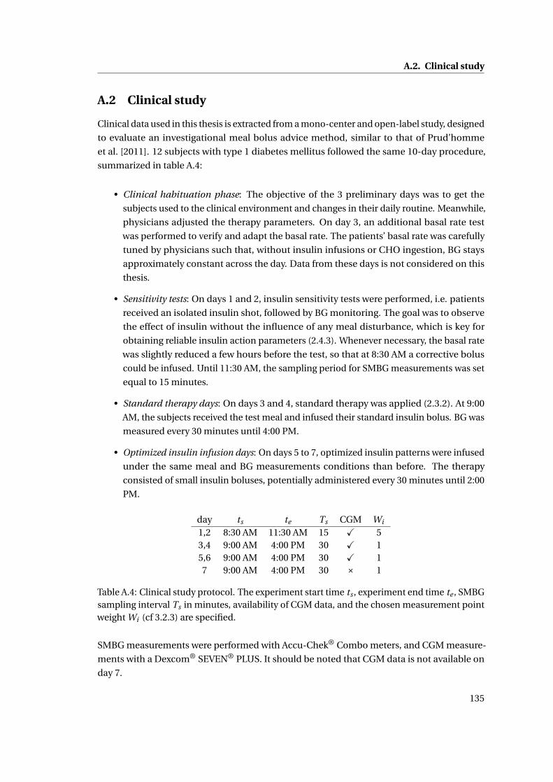
A.2. Clinical study
A.2 Clinical study
Clinical data used in this thesis is extracted from a mono-center and open-label study, designed
to evaluate an investigational meal bolus advice method, similar to that of Prud’homme
et al. [2011]. 12 subjects with type 1 diabetes mellitus followed the same 10-day procedure,
summarized in table A.4:
• Clinical habituation phase: The objective of the 3 preliminary days was to get the
subjects used to the clinical environment and changes in their daily routine. Meanwhile,
physicians adjusted the therapy parameters. On day 3, an additional basal rate test
was performed to verify and adapt the basal rate. The patients’ basal rate was carefully
tuned by physicians such that, without insulin infusions or CHO ingestion, BG stays
approximately constant across the day. Data from these days is not considered on this
thesis.
• Sensitivity tests: On days 1 and 2, insulin sensitivity tests were performed, i.e. patients
received an isolated insulin shot, followed by BG monitoring. The goal was to observe
the effect of insulin without the influence of any meal disturbance, which is key for
obtaining reliable insulin action parameters (2.4.3). Whenever necessary, the basal rate
was slightly reduced a few hours before the test, so that at 8:30 AM a corrective bolus
could be infused. Until 11:30 AM, the sampling period for SMBG measurements was set
equal to 15 minutes.
• Standard therapy days: On days 3 and 4, standard therapy was applied (2.3.2). At 9:00
AM, the subjects received the test meal and infused their standard insulin bolus. BG was
measured every 30 minutes until 4:00 PM.
• Optimized insulin infusion days: On days 5 to 7, optimized insulin patterns were infused
under the same meal and BG measurements conditions than before. The therapy
consisted of small insulin boluses, potentially administered every 30 minutes until 2:00
PM.
day ts te Ts CGM Wi
1,2 8:30 AM 11:30 AM 15 X 53,4 9:00 AM 4:00 PM 30 X 15,6 9:00 AM 4:00 PM 30 X 17 9:00 AM 4:00 PM 30 × 1
Table A.4: Clinical study protocol. The experiment start time ts , experiment end time te , SMBGsampling interval Ts in minutes, availability of CGM data, and the chosen measurement pointweight Wi (cf 3.2.3) are specified.
SMBG measurements were performed with Accu-Chek® Combo meters, and CGM measure-
ments with a Dexcom® SEVEN® PLUS. It should be noted that CGM data is not available on
day 7.
135
Appendix A. Validation data
The test meals were always the same fatty, heavy and long-lasting meals (750 kcal with 25-30%
carbohydrates, 15-20% protein, and 55-60% fat). This is a very slow acting meal, i.e. a meal
with low GI where the rise in BG is slow, chosen intentionally to show the benefits of an insulin
infusion pattern, which only exists if the insulin action is faster than the meal effect.
The following data were not considered for model validation:
• Data collected after a hypoglycemic intervention.
• Data collected after the intake of medication.
• Data with very high variability and unexplained BG excursions.
Of note is that this corresponds to the exclusion of 2 subjects. Overall, the standard therapy
parameter I2C was often underestimated leading to high BG concentrations, most likely due to
the slow nature of the selected meal. Therapy parameter values were updated on a day-to-day
basis. However, in this thesis, only one single therapy parameter value is considered per
patient.
The insulin sensitivity tests have a weight Wi that is 5 times the weight of the other days. This
increased importance given to the identification quality of the insulin subsystem is vital to
have a reliable identification of insulin action.
The data from this study are very well suited to analyze parameter correlations and compare
deterministic and stochastic model predictions since:
• insulin sensitivity tests were performed (cf. 2.4.3).
• the patients had the same meal several times on consecutive days, which prevents that
parameters change significantly over the course of the study.
• the basal rates and therapy parameters were very well adjusted by physicians.
• two different insulin infusion strategies were used.
The latter is interesting in that, generally speaking, if all study days are similar, models that
have good data fits generate good predictions even if they have inappropriate dynamics. On
the other hand, an even more diversified study design with, e.g., modified meal sizes, more
patients and more insulin sensitivity test days, would improve the quality of the data further.
136
B Metrics
In this thesis, many different metrics are used, in order to quantify the quality of data fits,
BG predictions and control performance. A good overview of many metrics is given by Del
Favero et al. [2012]. Additionally, Del Favero et al. propose an extension of existing metrics to
incorporate a glucose specific penalty, although this is not necessary in this thesis, since hypo-
and hyperglycemia conditions rarely occurred in the data sets. In the following sections, the
different metrics used along this document are introduced.
B.1 MAD
The MAD, in mg/dl, is used to compare data fits, as well as model predictions resulting from
the different investigated models. It is defined as:
MAD = 1
N
N∑t=1
|G(t )−G(t )| (B.1)
where N denotes the number of samples. It measures the mean absolute deviation between
an estimated and an exact BG concentration. Hence, the lower its value, the better the results.
B.2 R2
The coefficient of determination R2 in % is used to compare data fits, as well as model predic-
tions resulting from the different investigated models. It is defined as:
R2 = 100
(1−
1N
∑Nt=1(G(t )−G(t ))2
1N
∑Nt=1(G(t )−G)2
)(B.2)
where G is the average BG: G = 1N
∑Nt=1 G(t ). A value of 100% is equivalent to a perfect fit, while
bad fits may have negative values. This method is more sensitive to outliers, because of its
quadratic term.
137
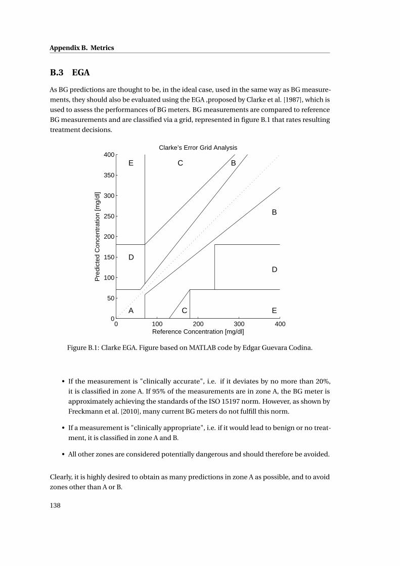
Appendix B. Metrics
B.3 EGA
As BG predictions are thought to be, in the ideal case, used in the same way as BG measure-
ments, they should also be evaluated using the EGA ,proposed by Clarke et al. [1987], which is
used to assess the performances of BG meters. BG measurements are compared to reference
BG measurements and are classified via a grid, represented in figure B.1 that rates resulting
treatment decisions.
0 100 200 300 4000
50
100
150
200
250
300
350
400
Reference Concentration [mg/dl]
Pre
dict
ed C
once
ntra
tion
[mg/
dl]
Clarke’s Error Grid Analysis
A
D
E C
C E
D
B
B
Figure B.1: Clarke EGA. Figure based on MATLAB code by Edgar Guevara Codina.
• If the measurement is "clinically accurate", i.e. if it deviates by no more than 20%,
it is classified in zone A. If 95% of the measurements are in zone A, the BG meter is
approximately achieving the standards of the ISO 15197 norm. However, as shown by
Freckmann et al. [2010], many current BG meters do not fulfill this norm.
• If a measurement is "clinically appropriate", i.e. if it would lead to benign or no treat-
ment, it is classified in zone A and B.
• All other zones are considered potentially dangerous and should therefore be avoided.
Clearly, it is highly desired to obtain as many predictions in zone A as possible, and to avoid
zones other than A or B.
138
B.4. BGRI
B.4 BGRI
The BGRI was introduced by Kovatchev et al. [2000] and is well recognized as a reliable
indicator of the clinical adequacy of a BG profile. As such the BGRI is implemented in the UVa
simulator as one of the main performance metrics. It is defined using a risk function r given
in equation B.4 and represented in figure 1.7.
f (G) = 1.509[(ln(G))1.084 −5.381
](B.3)
r (G) = 10 f (G)2 (B.4)
This function attributes a risk to every BG concentration G . The risk is zero at 112.5 mg/dl and
increases as G deviates from this target value. This increase is asymmetric as the risk during
hypoglycemia is higher than for hyperglycemia. Kovatchev et al. define the target BG range
between 70 and 180 mg/dl, which corresponds to a risk value of 7.7.
The BGRI is defined as the average r (G):
BGRI = 1
n
n∑i=1
r (Gi ) (B.5)
The BGRI can be split into HBGI and LBGI such that HBGI + LBGI = BGRI, where the contribu-
tions to the score come from values above or below the target of 112.5 mg/dl, respectively.
The BGRI is a very convenient tool to compare algorithms applied to the same experimental
scenarios. However, if the scenarios are different, the BGRI has little value.
As mentioned in section 5.3.4, Cameron et al. [2011] used a modified BGRI, proposed by Magni
et al. [2007], and defined by
f (G) = 3.5506[(ln(G))0.8353 −3.7932
](B.6)
r (G) = 10 f (G)2, (B.7)
for which zero risk is at 140 mg/dl.
B.5 RMSE
The RMSE, in mg/dl, is used to compare data fits, as well as model predictions resulting from
the different investigated models. It is defined as:
RMSE =√√√√ 1
N
N∑t=1
(G(t )−G(t ))2 (B.8)
139
Appendix B. Metrics
where N denotes the number of samples. It measures the square root of the mean square error
between an estimated and an exact BG concentration. Hence, the lower its value is, the better
are the results.
B.6 Percentage of time spent within a range of BG concentrations
A simple and comprehensive way to asses the controller performance is to compute the
percentage of time within given BG concentration ranges. Common ranges are:
• target range: 70-180 mg/dl. This is the range as much time as possible should be spent
in. This is in accordance with target defined by Kovatchev et al. [2000].
• hypoglycemia: < 70 mg/dl. Time spent below target should be minimized as there is an
increased risk of hypoglycemia.
• hyperglycemia: > 180 mg/dl. Time spend above target should be short in order to avoid
hyperglycemia.
• severe hypoglycemia ( < 50 mg/dl) should be avoided at all price since it puts patients
in acute danger.
B.7 Mean BG concentrations
The mean BG concentration over a complete data set, pre-meal, and post-meal are given
for some comparisons. The mean BG is an indicator of treatment performance, as a low
mean indicates that hyperglycemia was well avoided. However, it needs to be verified that
no hypoglycemia occurs. Mean pre- and post-meal BG concentrations should be low as well.
They allow getting more insight into how the treatment is when it comes to meal rejection and
target tracking. Average pre-meal BG corresponds to the average BG during the our preceding
the meal, while average post-meal BG is the average BG between the first and second hour
after the meal.
B.8 Minimum and maximum BG concentration
These metrics simply give the minimum and the maximum BG concentration during the
experiment. The minimum BG should be high, and most importantly greater than the hypo-
glycemic threshold, while the maximum should remain low. These two values are generally
used for the Control-Variability Grid Analysis (CVGA) introduced by Magni et al. [2008] and
modified by Soru et al. [2012], which plots the minimum and maximum against each other for
every patient in a population. However, this metric is not used in this thesis, because the 10
patient population is to small to lead to meaningful results.
140

B.9. Boxplot
B.9 Boxplot
Boxplots are used several times in this thesis to compare data from a certain number of
experiments. For each box, the central, red line is the median, the edges of the box are the
25th (q1) and 75th (q3) percentiles, the whiskers extend to the most extreme data points
not considered outliers, and outliers are plotted individually using red crosses. Points are
considered as outliers if they are larger than q3 +1.5(q3–q1) or smaller than q1–1.5(q3–q1).
141

C A Minimal Exercise Extension forModels of the Glucoregulatory System
In the context of this thesis, a model extension for the effect of exercise was developed and
published (Bock et al. [2011]). The development of this model is recalled and applied to the
new prediction models designed in chapter 2.
C.1 Introduction
Exercise can have lowering and increasing effects on BG concentrations and patients need to
adapt their treatment to stay within the above mentioned bounds if they want to exercise, as
explained by Zinman et al. [2004]. However, the necessary adaptions are difficult to estimate
and, thus, the risk of hypoglycemia is increased during exercise. In this context, models
predicting the effect of exercise can be very useful tools for helping patients to adjust their
treatment.
Only a few models for exercise are available in the literature, examples are Dalla Man et al.
[2009], Roy and Parker [2007], Kim et al. [2007], Hernández-Ordoñez and Campos-Delgado
[2008], Balakrishnan et al. [2013]. Their level of complexity varies strongly, but the number of
parameters is typically high, which makes their identification, using only BG measurements,
difficult.
For this reason, a minimal exercise extension for existing models of the glucoregulatory system
that is based on observations from a clinical study is proposed. This extension introduces
two additional parameters, that can be identified using only BG measurements, and one
intensity-independent exercise input. Patient specific parameters are shown to be necessary
to account for the considerable inter-patient variability.
This chapter is organized as follows: In Section C.2, the clinical study is described and analyzed.
The model extension and the parameter identification method are described in Section C.3.
Results are discussed in Section C.4, while conclusions are drawn in Section C.5.
143
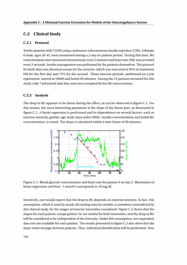
Appendix C. A Minimal Exercise Extension for Models of the Glucoregulatory System
C.2 Clinical Study
C.2.1 Protocol
Twelve patients with T1DM using continuous subcutaneous insulin injection (CSII), 6 female,
6 male, ages 20-45, were monitored during a 2-day in-patient period. During this time, BG
concentrations were measured intravenously every 5 minutes and heart rate (HR) was recorded
every 5 seconds. Insulin management was performed by the patients themselves. The protocol
for both days was identical except for the exercise, which was executed at 65% of maximum
HR for the first day and 75% for the second. These exercise periods, performed on cycle
ergometers, started at 16h00 and lasted 30 minutes. Among the 12 patients recruited for this
study, only 7 presented data that were not corrupted by low BG interventions.
C.2.2 Analysis
The drop in BG appears to be linear during the effort, as can be observed in figure C.1. For
this reason, the most interesting parameter is the slope of the linear part, as illustrated in
figure C.1. A linear regression is performed and its dependence on several factors, such as
exercise intensity, gender, age, body mass index (BMI), insulin concentrations and initial BG
concentrations, is tested. The slope is calculated within a time frame of 30 minutes.
0 15 30 45 60 75 903.5
4.25
5
5.75
6.5
7.25
8
Time (min)
Blo
od g
luco
se c
once
ntra
tion
(mm
ol/l)
0 15 30 45 60 75 9070
80
90
100
110
120
130
Hea
rt r
ate
(BP
M)
Exercise start
Figure C.1: Blood glucose concentration and heart rate for patient 9 on day 2. Illustration oflinear regression (red line). 1 mmol/l corresponds to 18 mg/dl.
Intuitively, one would expect that the drop in BG depends on exercise intensity. In fact, this
assumption, which is used by nearly all existing exercise models, is somehow contradicted by
this clinical study, for the ranges of exercise intensities considered. Figure C.2 shows that the
slopes for each patient, except patient 10, are similar for both intensities, and the drop in BG
will be considered to be independent of the intensity. Under this assumption, two equivalent
data sets are available for each patient. The results presented in figure C.2 also show that the
slope varies strongly between patients. Thus, individual identification will be performed. Note
144
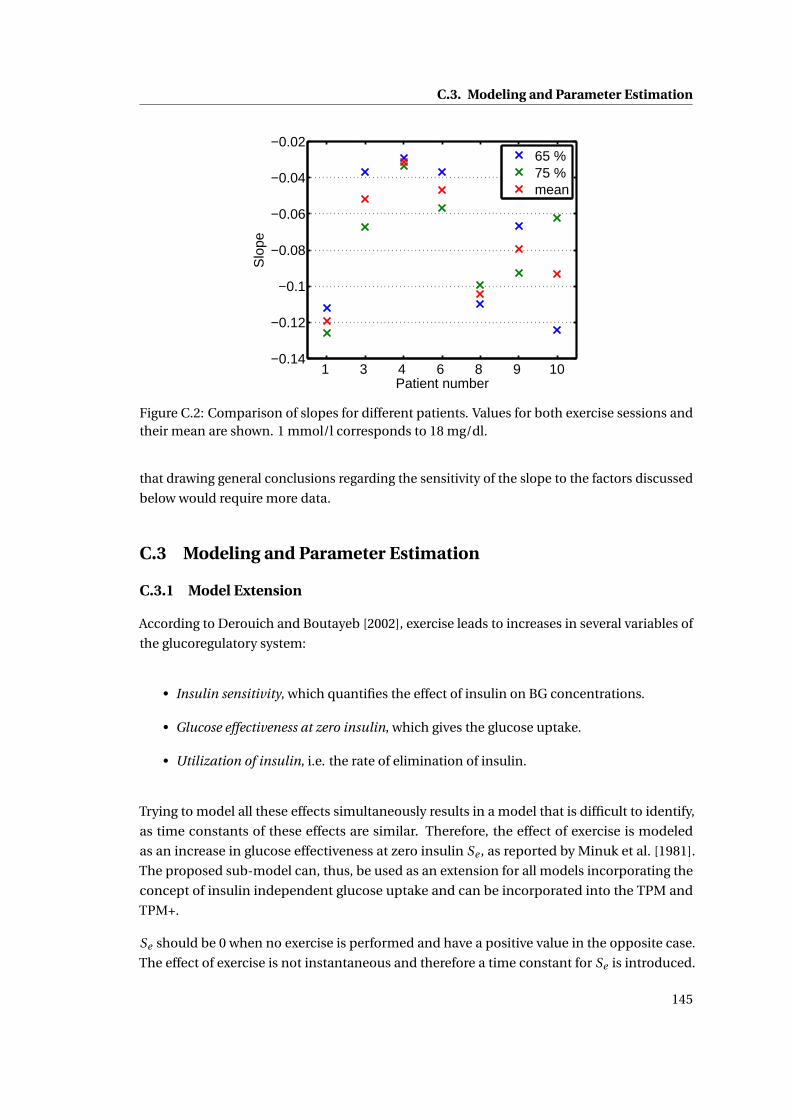
C.3. Modeling and Parameter Estimation
1 3 4 6 8 9 10−0.14
−0.12
−0.1
−0.08
−0.06
−0.04
−0.02
Patient number
Slo
pe
65 %75 %mean
Figure C.2: Comparison of slopes for different patients. Values for both exercise sessions andtheir mean are shown. 1 mmol/l corresponds to 18 mg/dl.
that drawing general conclusions regarding the sensitivity of the slope to the factors discussed
below would require more data.
C.3 Modeling and Parameter Estimation
C.3.1 Model Extension
According to Derouich and Boutayeb [2002], exercise leads to increases in several variables of
the glucoregulatory system:
• Insulin sensitivity, which quantifies the effect of insulin on BG concentrations.
• Glucose effectiveness at zero insulin, which gives the glucose uptake.
• Utilization of insulin, i.e. the rate of elimination of insulin.
Trying to model all these effects simultaneously results in a model that is difficult to identify,
as time constants of these effects are similar. Therefore, the effect of exercise is modeled
as an increase in glucose effectiveness at zero insulin Se , as reported by Minuk et al. [1981].
The proposed sub-model can, thus, be used as an extension for all models incorporating the
concept of insulin independent glucose uptake and can be incorporated into the TPM and
TPM+.
Se should be 0 when no exercise is performed and have a positive value in the opposite case.
The effect of exercise is not instantaneous and therefore a time constant for Se is introduced.
145
Appendix C. A Minimal Exercise Extension for Models of the Glucoregulatory System
The dynamic behavior of Se is defined in equation (C.1).
Se (t ) =−ae Se (t )+Ke aeUe (t ) (C.1)
Where ae (the inverse of the time constant in min−1) and Ke (the exercise sensitivity in min−1)
are the two additional parameters that have been introduced.
As a consequence of the independence on exercise intensity, the new input Ue = 0 if no exercise
is performed and 1 otherwise, and thus, Ke represents the amplitude of the increase in glucose
uptake, while ae shows how fast the effect appears and disappears.
C.3.2 Parameter Identification
An appropriate model of the glucoregulatory system is needed to identify the resulting new
parameters. A modified version of the BMM is used. During exercise, the insulin infusion is
constant. Therefore, the effect of insulin is considered constant during this period and can
be combined with the glucose effectiveness at zero insulin into the new parameter Si ns+G .
Endogenous glucose production is assumed to be constant during exercise (Minuk et al.
[1981]). The complete model extension corresponds to equations (C.1) and (C.2).
G(t ) =− (Si ns+G +Se (t ))G(t )+Si ns+GGb (C.2)
Where G is the BG in mg/dl and Gb is the basal BG chosen equal to 100 mg/dl. The term
Si ns+GGb is the endogenous glucose production.
Firstly, Si ns+G is identified for each day and each patient using the data collected before the
exercise session, and a standard least squares approach. This allows taking into account
differences in insulin infusion that may occur from one day to another.
Then, in a second step, ae and Ke are identified using the Iterative Two Stage (ITS) method
(Vicini and Cobelli [2001]). As the exercise effect is supposed to be identical for the two days,
only one couple (ae , Ke ) is identified for each patient.
However, as the sensitivity for ae is low, an empirical value can be chosen without loss of
prediction capabilities, as shown in figure C.3, and better coefficients of variation are obtained.
A value of 0.1 min−1 is proposed.
146
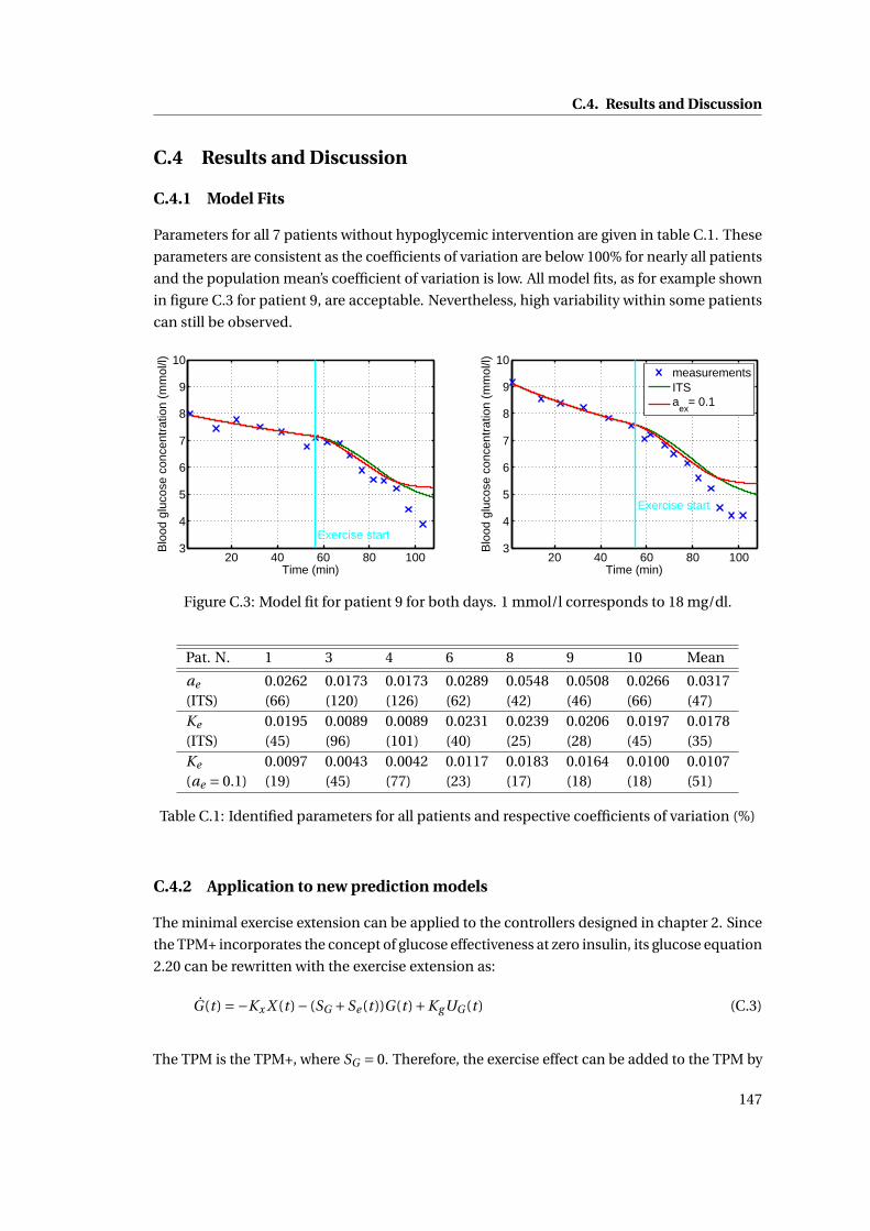
C.4. Results and Discussion
C.4 Results and Discussion
C.4.1 Model Fits
Parameters for all 7 patients without hypoglycemic intervention are given in table C.1. These
parameters are consistent as the coefficients of variation are below 100% for nearly all patients
and the population mean’s coefficient of variation is low. All model fits, as for example shown
in figure C.3 for patient 9, are acceptable. Nevertheless, high variability within some patients
can still be observed.
20 40 60 80 1003
4
5
6
7
8
9
10
Time (min)
Blo
od g
luco
se c
once
ntra
tion
(mm
ol/l)
Exercise start
20 40 60 80 1003
4
5
6
7
8
9
10
Time (min)
Blo
od g
luco
se c
once
ntra
tion
(mm
ol/l)
Exercise start
measurementsITSa
ex= 0.1
Figure C.3: Model fit for patient 9 for both days. 1 mmol/l corresponds to 18 mg/dl.
Pat. N. 1 3 4 6 8 9 10 Mean
ae 0.0262 0.0173 0.0173 0.0289 0.0548 0.0508 0.0266 0.0317(ITS) (66) (120) (126) (62) (42) (46) (66) (47)Ke 0.0195 0.0089 0.0089 0.0231 0.0239 0.0206 0.0197 0.0178(ITS) (45) (96) (101) (40) (25) (28) (45) (35)Ke 0.0097 0.0043 0.0042 0.0117 0.0183 0.0164 0.0100 0.0107(ae = 0.1) (19) (45) (77) (23) (17) (18) (18) (51)
Table C.1: Identified parameters for all patients and respective coefficients of variation (%)
C.4.2 Application to new prediction models
The minimal exercise extension can be applied to the controllers designed in chapter 2. Since
the TPM+ incorporates the concept of glucose effectiveness at zero insulin, its glucose equation
2.20 can be rewritten with the exercise extension as:
G(t ) =−Kx X (t )− (SG +Se (t ))G(t )+KgUG (t ) (C.3)
The TPM is the TPM+, where SG = 0. Therefore, the exercise effect can be added to the TPM by
147
Appendix C. A Minimal Exercise Extension for Models of the Glucoregulatory System
modifying the BG equation 2.14:
G(t ) =−Kx X (t )+KgUG (t )−Se (t )G(t ) (C.4)
C.4.3 Model Limitations
The proposed model extension is strongly based on observations collected during a clinical
study. However, this study only covers a small subset of possible exercise setups in terms of
exercise duration or intensity and exercise types.
• Because exercise duration was 30 minutes, the extension is only applicable for exercise
with limited durations. In fact, after about 90 minutes, the physiological processes
change since the hepatic glycogen stocks are depleted Ahlborg et al. [1974]. Hence, the
exercise effects are no longer captured by the proposed extension after 90 minutes.
• The exercise intensity was set to 65 and 75% of the maximal heart rate, i.e. in the
aerobic range. However, at higher intensities, the anaerobic threshold is passed and BG
dynamics change Marliss and Vranic [2002].
• The type of exercise that is performed might change the exercise parameters. As only
data from cycling are available, this cannot be verified.
• The middle and long term effects of exercise on insulin sensitivity are not taken into
account in this extension. However, it is shown that these changes in insulin sensitivity
can be detected up to 2 days after the exercise session Mikines et al. [1988], but also over
several weeks when regular exercise is performed Nishida et al. [2004].
C.5 Conclusion
A model extension for predicting the evolution of BG concentrations during exercise has
been proposed. This model was found to be identifiable and in accordance with the clinical
study. Additionally, as the exercise input is independent of exercise intensity, no additional
measurement device is necessary. Implementations should lead to an improved quality of life
for patients suffering from T1DM. Future work will include an extension of the proposed model
to longer durations and a broader range of exercise intensities. For this purpose, additional
clinical studies will have to be carried out. The performance of the exercise extension on the
TPM and TPM+ would need to be tested as well. The alternative model, following the TPM
principles can be tested as well. If the insulin and meal sub-models are not considered, the
equations are
G(t ) =−Se (t ) (C.5)
Se (t ) =−ae Se (t )+ae Se,1(t ) (C.6)
Se,1(t ) =−ae Se,1(t )+aeUe (t ). (C.7)
148
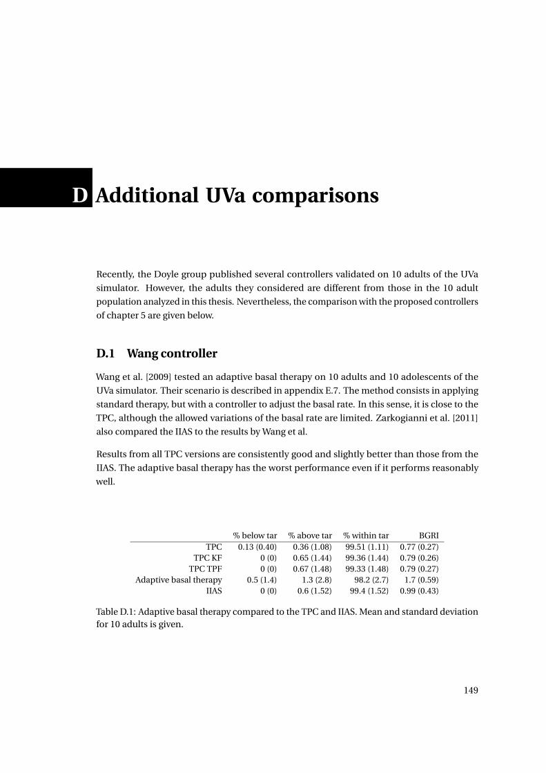
D Additional UVa comparisons
Recently, the Doyle group published several controllers validated on 10 adults of the UVa
simulator. However, the adults they considered are different from those in the 10 adult
population analyzed in this thesis. Nevertheless, the comparison with the proposed controllers
of chapter 5 are given below.
D.1 Wang controller
Wang et al. [2009] tested an adaptive basal therapy on 10 adults and 10 adolescents of the
UVa simulator. Their scenario is described in appendix E.7. The method consists in applying
standard therapy, but with a controller to adjust the basal rate. In this sense, it is close to the
TPC, although the allowed variations of the basal rate are limited. Zarkogianni et al. [2011]
also compared the IIAS to the results by Wang et al.
Results from all TPC versions are consistently good and slightly better than those from the
IIAS. The adaptive basal therapy has the worst performance even if it performs reasonably
well.
% below tar % above tar % within tar BGRITPC 0.13 (0.40) 0.36 (1.08) 99.51 (1.11) 0.77 (0.27)
TPC KF 0 (0) 0.65 (1.44) 99.36 (1.44) 0.79 (0.26)TPC TPF 0 (0) 0.67 (1.48) 99.33 (1.48) 0.79 (0.27)
Adaptive basal therapy 0.5 (1.4) 1.3 (2.8) 98.2 (2.7) 1.7 (0.59)IIAS 0 (0) 0.6 (1.52) 99.4 (1.52) 0.99 (0.43)
Table D.1: Adaptive basal therapy compared to the TPC and IIAS. Mean and standard deviationfor 10 adults is given.
149
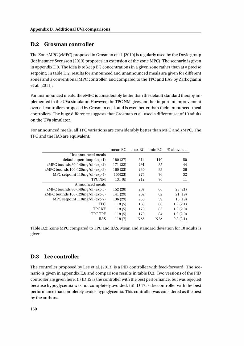
Appendix D. Additional UVa comparisons
D.2 Grosman controller
The Zone MPC (zMPC) proposed in Grosman et al. [2010] is regularly used by the Doyle group
(for instance Svensson [2013] proposes an extension of the zone MPC). The scenario is given
in appendix E.8. The idea is to keep BG concentrations in a given zone rather than at a precise
setpoint. In table D.2, results for announced and unannounced meals are given for different
zones and a conventional MPC controller, and compared to the TPC and IIAS by Zarkogianni
et al. [2011].
For unannounced meals, the zMPC is considerably better than the default standard therapy im-
plemented in the UVa simulator. However, the TPC NM gives another important improvement
over all controllers proposed by Grosman et al. and is even better than their announced-meal
controllers. The huge difference suggests that Grosman et al. used a different set of 10 adults
on the UVa simulator.
For announced meals, all TPC variations are considerably better than MPC and zMPC. The
TPC and the IIAS are equivalent.
mean BG max BG min BG % above tarUnannounced meals
default open-loop (exp 1) 180 (27) 314 110 50zMPC bounds 80-140mg/dl (exp 2) 171 (22) 291 85 44
zMPC bounds 100-120mg/dl (exp 3) 160 (23) 280 83 36MPC setpoint 110mg/dl (exp 4) 155(23) 274 76 32
TPC NM 131 (6) 212 76 11Announced meals
zMPC bounds 80-140mg/dl (exp 5) 152 (28) 267 66 28 (21)zMPC bounds 100-120mg/dl (exp 6) 141 (29) 262 62 21 (19)
MPC setpoint 110mg/dl (exp 7) 136 (29) 258 59 18 (19)TPC 118 (5) 169 80 1.2 (2.1)
TPC KF 118 (5) 170 83 1.2 (2.0)TPC TPF 118 (5) 170 84 1.2 (2.0)
IIAS 118 (7) N/A N/A 0.8 (2.1)
Table D.2: Zone MPC compared to TPC and IIAS. Mean and standard deviation for 10 adults isgiven.
D.3 Lee controller
The controller proposed by Lee et al. [2013] is a PID controller with feed-forward. The sce-
nario is given in appendix E.6 and comparison results in table D.3. Two versions of the PID
controller are given here: (i) ID 12 is the controller with the best performance, but was rejected
because hypoglycemia was not completely avoided. (ii) ID 17 is the controller with the best
performance that completely avoids hypoglycemia. This controller was considered as the best
by the authors.
150
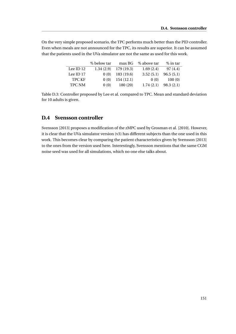
D.4. Svensson controller
On the very simple proposed scenario, the TPC performs much better than the PID controller.
Even when meals are not announced for the TPC, its results are superior. It can be assumed
that the patients used in the UVa simulator are not the same as used for this work.
% below tar max BG % above tar % in tarLee ID 12 1.34 (2.9) 179 (19.3) 1.69 (2.4) 97 (4.4)Lee ID 17 0 (0) 183 (19.6) 3.52 (5.1) 96.5 (5.1)
TPC KF 0 (0) 154 (12.1) 0 (0) 100 (0)TPC NM 0 (0) 180 (20) 1.74 (2.1) 98.3 (2.1)
Table D.3: Controller proposed by Lee et al. compared to TPC. Mean and standard deviationfor 10 adults is given.
D.4 Svensson controller
Svensson [2013] proposes a modification of the zMPC used by Grosman et al. [2010]. However,
it is clear that the UVa simulator version (v3) has different subjects than the one used in this
work. This becomes clear by comparing the patient characteristics given by Svensson [2013]
to the ones from the version used here. Interestingly, Svensson mentions that the same CGM
noise seed was used for all simulations, which no one else talks about.
151

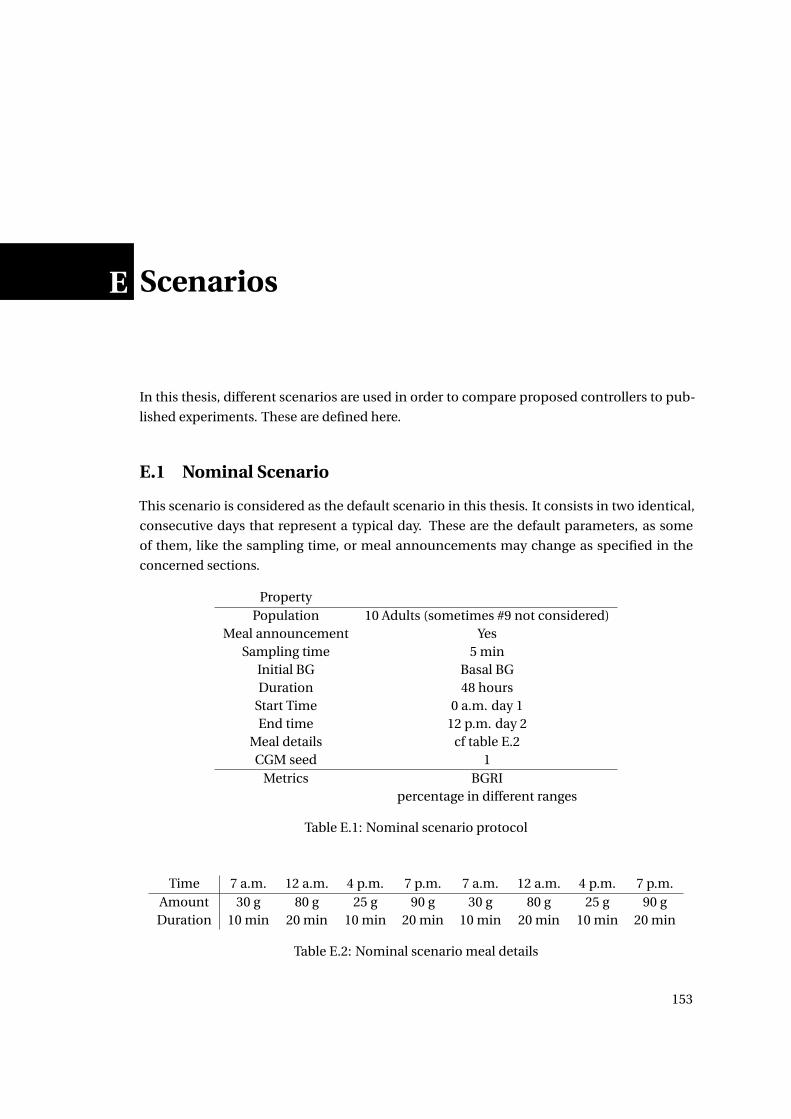
E Scenarios
In this thesis, different scenarios are used in order to compare proposed controllers to pub-
lished experiments. These are defined here.
E.1 Nominal Scenario
This scenario is considered as the default scenario in this thesis. It consists in two identical,
consecutive days that represent a typical day. These are the default parameters, as some
of them, like the sampling time, or meal announcements may change as specified in the
concerned sections.
PropertyPopulation 10 Adults (sometimes #9 not considered)
Meal announcement YesSampling time 5 min
Initial BG Basal BGDuration 48 hours
Start Time 0 a.m. day 1End time 12 p.m. day 2
Meal details cf table E.2CGM seed 1
Metrics BGRIpercentage in different ranges
Table E.1: Nominal scenario protocol
Time 7 a.m. 12 a.m. 4 p.m. 7 p.m. 7 a.m. 12 a.m. 4 p.m. 7 p.m.Amount 30 g 80 g 25 g 90 g 30 g 80 g 25 g 90 gDuration 10 min 20 min 10 min 20 min 10 min 20 min 10 min 20 min
Table E.2: Nominal scenario meal details
153

Appendix E. Scenarios
E.2 Zarkogianni Scenario
Zarkogianni et al. [2011] use a non linear MPC with a double deterministic model and Neural
Network coupled to a fuzzy logic adaptive scheme to control blood glucose. Their scenario is
summarized in tables E.3 and E.4.
PropertyPopulation 10 Adults
Meal announcement YesSampling time 5 min
Initial BG Basal BG (supposedly)Duration 48 hours
Start Time 0 a.m. day 1End time 12 p.m. day 2
Meal duration 15 min (5 min for 5g meal) (not specified)Meal details cf table E.4
Metrics % in different regionsLBGI, HBGI, BGRI
population mean and standard deviation
Table E.3: Zarkogianni scenario protocol
Time 7 a.m. 12 a.m. 4 p.m. 6 p.m. 11 p.m. 7:30 a.m. 1 p.m. 6:30 p.m.Amount 45 g 70 g 5 g 80 g 5 g 40 g 85 g 60 g
Table E.4: Zarkogianni scenario meal details
E.3 Cameron Scenario
Cameron et al. [2011] tested their MPC controller on the scenario specified in tables E.5 and
E.6.
E.4 Cormerais Scenario 1 day
Cormerais and Richard [2012] use two different scenarios, one of which is a one day scenario
specified in tables E.7 and E.8.
E.5 Cormerais Scenario 7 days
The second scenario used in Cormerais and Richard [2012] is specified in table E.9. This
scenario is quite complex with very diverse meal times and amounts. For the complete
schedule, please refer to the article.
154
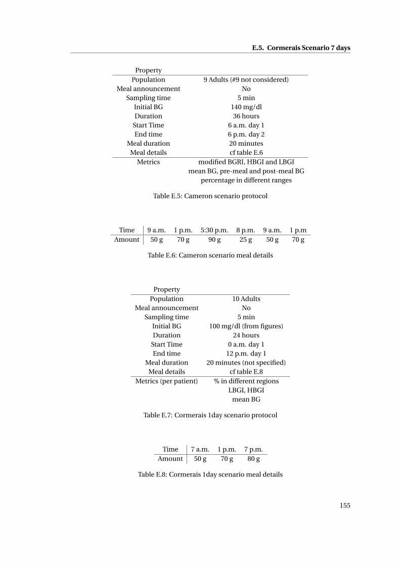
E.5. Cormerais Scenario 7 days
PropertyPopulation 9 Adults (#9 not considered)
Meal announcement NoSampling time 5 min
Initial BG 140 mg/dlDuration 36 hours
Start Time 6 a.m. day 1End time 6 p.m. day 2
Meal duration 20 minutesMeal details cf table E.6
Metrics modified BGRI, HBGI and LBGImean BG, pre-meal and post-meal BG
percentage in different ranges
Table E.5: Cameron scenario protocol
Time 9 a.m. 1 p.m. 5:30 p.m. 8 p.m. 9 a.m. 1 p.mAmount 50 g 70 g 90 g 25 g 50 g 70 g
Table E.6: Cameron scenario meal details
PropertyPopulation 10 Adults
Meal announcement NoSampling time 5 min
Initial BG 100 mg/dl (from figures)Duration 24 hours
Start Time 0 a.m. day 1End time 12 p.m. day 1
Meal duration 20 minutes (not specified)Meal details cf table E.8
Metrics (per patient) % in different regionsLBGI, HBGI
mean BG
Table E.7: Cormerais 1day scenario protocol
Time 7 a.m. 1 p.m. 7 p.m.Amount 50 g 70 g 80 g
Table E.8: Cormerais 1day scenario meal details
155

Appendix E. Scenarios
PropertyPopulation 10 Adults
Meal announcement NoSampling time 5 min
Initial BG 100 mg/dl (from figures)Duration 7 days
Start Time 0 a.m. day 1End time 12 p.m. day 7
Meal duration 20 minutes (not specified)Meal details cf table Cormerais and Richard [2012]
Metrics (per patient) % in different regionsLBGI, HBGI
mean BG
Table E.9: Cormerais 7day scenario protocol
E.6 Lee Scenario
Lee et al. [2013] tested their PID controller on the following scenario. Details are given in table
E.10 and E.11.
PropertyPopulation 10 Adults
Meal announcement YesSampling time 5 min
Initial BG Basal BG (supposedly)Duration 31 hours
Start Time 0 a.m. day 1End time 7 a.m. day 2
Meal duration 20 minutes (not specified)Meal details cf table E.11
Metrics % in different regionsmaximum BG
population mean and standard deviation
Table E.10: Lee scenario protocol
Time 7 a.m.Amount 50 g
Table E.11: Lee scenario meal details
156
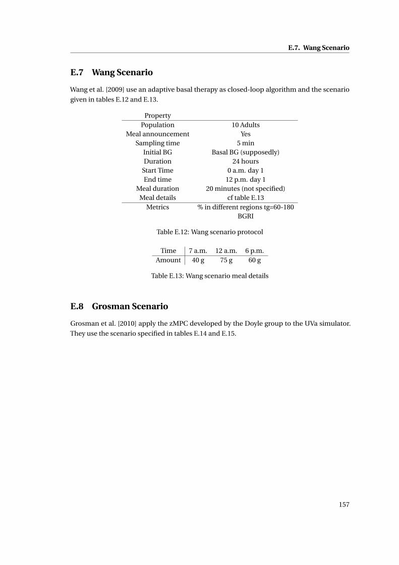
E.7. Wang Scenario
E.7 Wang Scenario
Wang et al. [2009] use an adaptive basal therapy as closed-loop algorithm and the scenario
given in tables E.12 and E.13.
PropertyPopulation 10 Adults
Meal announcement YesSampling time 5 min
Initial BG Basal BG (supposedly)Duration 24 hours
Start Time 0 a.m. day 1End time 12 p.m. day 1
Meal duration 20 minutes (not specified)Meal details cf table E.13
Metrics % in different regions tg=60-180BGRI
Table E.12: Wang scenario protocol
Time 7 a.m. 12 a.m. 6 p.m.Amount 40 g 75 g 60 g
Table E.13: Wang scenario meal details
E.8 Grosman Scenario
Grosman et al. [2010] apply the zMPC developed by the Doyle group to the UVa simulator.
They use the scenario specified in tables E.14 and E.15.
157
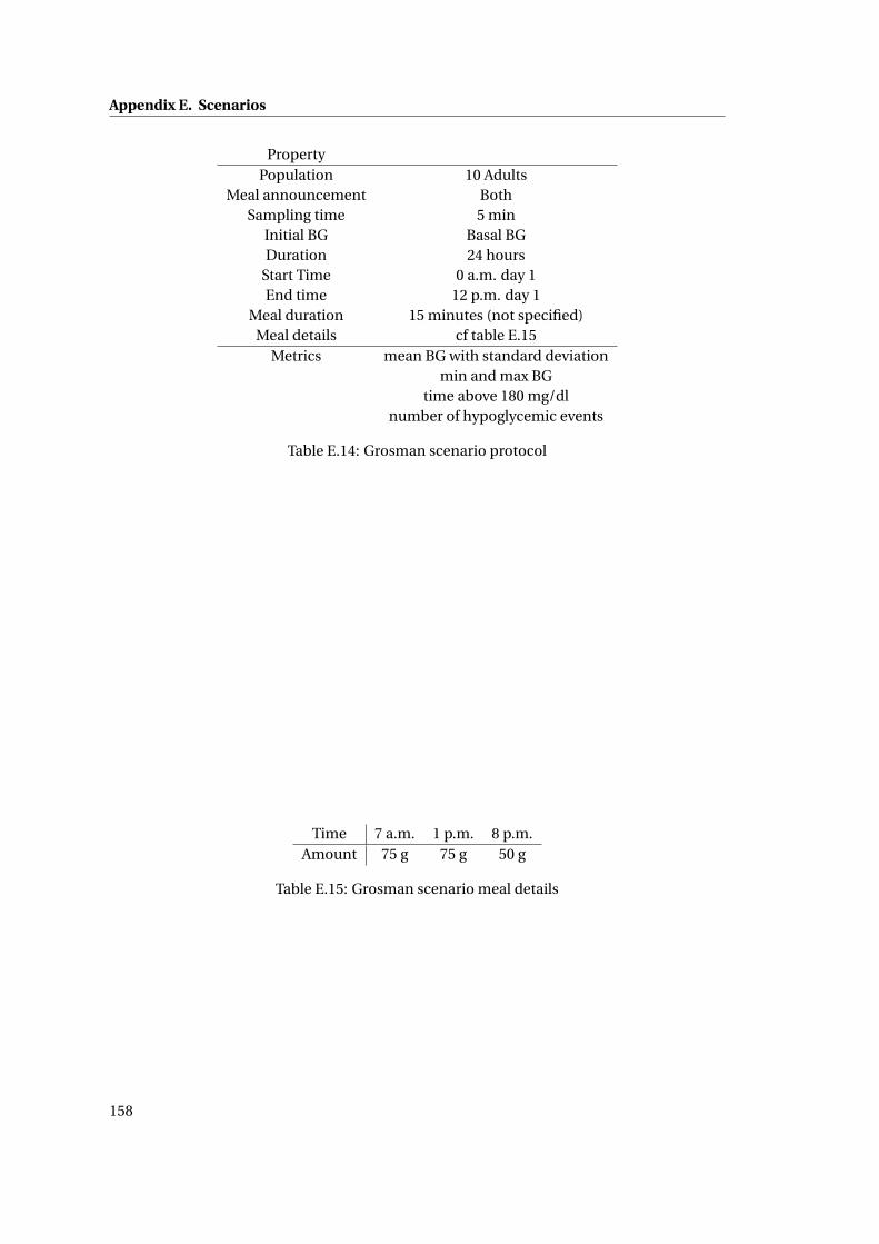
Appendix E. Scenarios
PropertyPopulation 10 Adults
Meal announcement BothSampling time 5 min
Initial BG Basal BGDuration 24 hours
Start Time 0 a.m. day 1End time 12 p.m. day 1
Meal duration 15 minutes (not specified)Meal details cf table E.15
Metrics mean BG with standard deviationmin and max BG
time above 180 mg/dlnumber of hypoglycemic events
Table E.14: Grosman scenario protocol
Time 7 a.m. 1 p.m. 8 p.m.Amount 75 g 75 g 50 g
Table E.15: Grosman scenario meal details
158
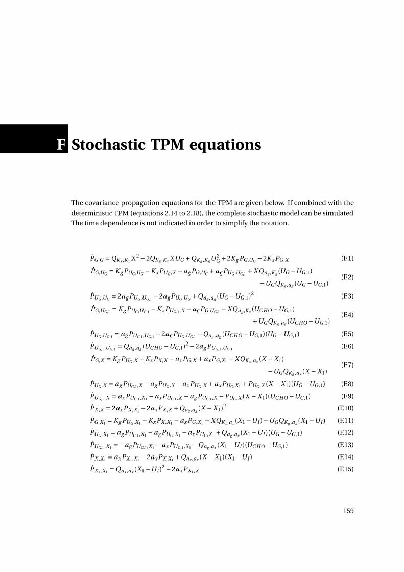
F Stochastic TPM equations
The covariance propagation equations for the TPM are given below. If combined with the
deterministic TPM (equations 2.14 to 2.18), the complete stochastic model can be simulated.
The time dependence is not indicated in order to simplify the notation.
PG ,G =QKx ,Kx X 2 −2QKg ,Kx XUG +QKg ,Kg U 2G +2Kg PG ,UG −2Kx PG ,X (F.1)
PG ,UG = Kg PUG ,UG −Kx PUG ,X −ag PG ,UG +ag PUG ,UG ,1 +X Qag ,Kx (UG −UG ,1)
−UGQKg ,ag (UG −UG ,1)(F.2)
PUG ,UG = 2ag PUG ,UG ,1 −2ag PUG ,UG +Qag ,ag (UG −UG ,1)2 (F.3)
PG ,UG ,1 = Kg PUG ,UG ,1 −Kx PUG ,1,X −ag PG ,UG ,1 −XQag ,Kx (UC HO −UG ,1)
+UGQKg ,ag (UC HO −UG ,1)(F.4)
PUG ,UG ,1 = ag PUG ,1,UG ,1 −2ag PUG ,UG ,1 −Qag ,ag (UC HO −UG ,1)(UG −UG ,1) (F.5)
PUG ,1,UG ,1 =Qag ,ag (UC HO −UG ,1)2 −2ag PUG ,1,UG ,1 (F.6)
PG ,X = Kg PUG ,X −Kx PX ,X −ax PG ,X +ax PG ,X1 +XQKx ,ax (X −X1)
−UGQKg ,ax (X −X1)(F.7)
PUG ,X = ag PUG ,1,X −ag PUG ,X −ax PUG ,X +ax PUG ,X1 +PUG ,X (X −X1)(UG −UG ,1) (F.8)
PUG ,1,X = ax PUG ,1,X1 −ax PUG ,1,X −ag PUG ,1,X −PUG ,X (X −X1)(UC HO −UG ,1) (F.9)
PX ,X = 2ax PX ,X1 −2ax PX ,X +Qax ,ax (X −X1)2 (F.10)
PG ,X1 = Kg PUG ,X1 −Kx PX ,X1 −ax PG ,X1 +XQKx ,ax (X1 −UI )−UGQKg ,ax (X1 −UI ) (F.11)
PUG ,X1 = ag PUG ,1,X1 −ag PUG ,X1 −ax PUG ,X1 +Qag ,ax (X1 −UI )(UG −UG ,1) (F.12)
PUG ,1,X1 =−ag PUG ,1,X1 −ax PUG ,1,X1 −Qag ,ax (X1 −UI )(UC HO −UG ,1) (F.13)
PX ,X1 = ax PX1,X1 −2ax PX , X1 +Qax ,ax (X −X1)(X1 −UI ) (F.14)
PX1,X1 =Qax ,ax (X1 −UI )2 −2ax PX1,X1 (F.15)
159

Bibliography
Amjad Abu-Rmileh and Winston Garcia-Gabin. Wiener sliding-mode control for artificial
pancreas: A new nonlinear approach to glucose regulation. Comput. Methods Programs
Biomed., pages 1–14, May 2012. ISSN 1872-7565. doi: 10.1016/j.cmpb.2012.03.001.
G Ahlborg, P Felig, L Hagenfeldt, R Hendler, and J Wahren. Substrate Turnover during Pro-
longed Exercise in Man. Splanchnic and leg metabolism of glucose, free fatty acids, and
amino acids. J Clin Invest, 53(4):1080–1090, 1974. ISSN 0021-9738.
Naviyn Prabhu Balakrishnan, Gade Pandu Rangaiah, and Lakshminarayanan Samavedham.
Review and Analysis of Blood Glucose (BG) Models for Type 1 Diabetic Patients. Ind. Eng.
Chem. Res., 50(21):12041–12066, November 2011. ISSN 0888-5885. doi: 10.1021/ie2004779.
URL http://pubs.acs.org/doi/abs/10.1021/ie2004779.
Naviyn Prabhu Balakrishnan, Lakshminarayanan Samavedham, and Gade Pandu Rangaiah.
Personalized Hybrid Models for Exercise, Meal and Insulin Interventions in Type 1 Diabetic
Children and Adolescents. Ind. Eng. Chem. Res., August 2013. ISSN 0888-5885. doi: 10.1021/
ie402531k. URL http://pubs.acs.org/doi/abs/10.1021/ie402531k.
F G Banting, C H Best, J B Collip, W R Campbell, and A A Fletcher. Pancreatic Extracts in
the Treatment of Diabetes Mellitus. Can. Med. Assoc. J., 12(3):141–6, March 1922. ISSN
0008-4409. URL http://www.ncbi.nlm.nih.gov/pubmed/17580419.
Ananda Basu, Simmi Dube, Michael Slama, Isabel Errazuriz, Jose Carlos Amezcua, Yogish C
Kudva, Thomas Peyser, Rickey E Carter, Claudio Cobelli, and Rita Basu. Time Lag of Glucose
from Intravascular to Interstitial Compartment in Humans. Diabetes, pages 1–21, 2013.
B Wayne Bequette. Challenges and recent progress in the development of a closed-loop artifi-
cial pancreas. Annu. Rev. Control, October 2012. ISSN 13675788. doi: 10.1016/j.arcontrol.
2012.09.007. URL http://linkinghub.elsevier.com/retrieve/pii/S1367578812000429.
R N Bergman, Y Z Ider, C R Bowden, and C Cobelli. Quantitative estimation of insulin sensitivity.
Am J Physiol Gastrointest Liver Physiol, 236(6):G667–677, 1979.
R N Bergman, L S Phillips, and C Cobelli. Physiologic Evaluation of Factors Controlling Glucose
Tolerance in Man. J Clin Invest, 68(November 1981):1456–1467, 1981.
161
Bibliography
A Bock, G François, T Prud’homme, and D Gillet. A Minimal Exercise Extension for Models
of the Glucoregulatory System. In Comput. Aided Chem. Eng., pages 1520–1524. 2011. doi:
10.1016/B978-0-444-54298-4.50083-0.
A Bock, G François, and D Gillet. A Therapy Parameter-based Model for Predicting Blood
Glucose Concentrations in Patients with Type 1 Diabetes. Comput. Methods Programs
Biomed., 2013.
D Boiroux, D A Finan, J Bagterp Jørgensen, N Kjølstad Poulsen, and H Madsen. Optimal Insulin
Administration for People with Type 1 Diabetes. Number Dycops, pages 234–239, Leuven,
2010a.
D Boiroux, D A Finan, J B Jø rgensen, N K Poulsen, and H Madsen. Meal Estimation in Nonlinear
Model Predictive Control for Type 1 Diabetes. In Symp. Nonlinear Control Syst., pages
1052–1057, 2010b. URL http://scholar.google.com/scholar?hl=en&btnG=Search&q=intitle:
Meal+Estimation+in+Nonlinear+Model+Predictive+Control+for+Type+1+Diabetes#8.
J Bondia, A J Laguna, P Rossetti, F J Ampudia-Blasco, and J Vehí. On the use of hard/soft
specifications to deal with intra-patient variability in postprandial glucose control in type 1
diabetes. In 18th IFAC World Congr., volume 1, pages 8347–53, Milano, 2011.
M Breton. Physical Activity - The Major Unaccounted Impediment to Closed Loop Control. J.
Diabetes Sci. Technol., 2:169–174, 2008.
M Breton and B P Kovatchev. Analysis, modeling, and simulation of the accuracy of continuous
glucose sensors. J. Diabetes Sci. Technol., 2(5):853–62, September 2008. ISSN 1932-2968.
Razvan Bunescu, Nigel Struble, Cindy Marling, Jay Shubrook, and Frank Schwartz. Blood
Glucose Level Prediction using Physiological Models and Support Vector Regression. ouc-
sace.cs.ohiou.edu, 2013. URL http://oucsace.cs.ohiou.edu/~razvan/papers/icmla13.pdf.
F Cameron. Explicitly Minimizing Clinical Risk through Closed-loop Control of Blood Glucose
in Patients with Type 1 Diabetes Mellitus. PhD thesis, Stanford University, 2010.
Fraser Cameron, Günter Niemeyer, Karen Gundy-Burlet, and Bruce Buckingham. Statistical
hypoglycemia prediction. J. Diabetes Sci. Technol., 2(4):612–21, July 2008. ISSN 1932-2968.
Fraser Cameron, B W Bequette, D M Wilson, B A Buckingham, H Lee, and G Niemeyer. A
Closed-Loop Artificial Pancreas Based on Risk Management. J. Diabetes Sci. Technol., 5(2):
368–379, 2011.
Fraser Cameron, Darrell M Wilson, Bruce A Buckingham, Hasmik Arzumanyan, Paula Clinton,
H Peter Chase, John Lum, David M Maahs, Peter M Calhoun, and B Wayne Bequette. Inpa-
tient studies of a Kalman-filter-based predictive pump shutoff algorithm. J. Diabetes Sci.
Technol., 6(5):1142–7, September 2012. ISSN 1932-2968. URL http://www.pubmedcentral.
nih.gov/articlerender.fcgi?artid=3570849&tool=pmcentrez&rendertype=abstract.
162

Bibliography
Germán Campetelli, Mercedes Lombarte, Marta S. Basualdo, and Alfredo Rigalli. Extended
Adaptive Predictive Controller with Robust Filter to Enhance Blood Glucose Regulation
in Type I Diabetic Subjects. Comput. Chem. Eng., June 2013. ISSN 00981354. doi:
10.1016/j.compchemeng.2013.06.012. URL http://linkinghub.elsevier.com/retrieve/pii/
S0098135413002068.
Ismael Capel, Mercedes Rigla, Gema García-Sáez, Agustín Rodríguez-Herrero, Belén Pons,
David Subías, Fernando García-García, Maria Gallach, Montserrat Aguilar, Carmen Pérez-
Gandía, Enrique J Gómez, Assumpta Caixàs, and M Elena Hernando. Artificial Pancreas
Using a Personalized Rule-Based Controller Achieves Overnight Normoglycemia in Patients
with Type 1 Diabetes. Diabetes Technol. Ther., 16(3):3–10, October 2013. ISSN 1557-8593.
doi: 10.1089/dia.2013.0229. URL http://www.ncbi.nlm.nih.gov/pubmed/24152323.
Marzia Cescon. Linear Modeling and Prediction in Diabetes Physiology. PhD thesis, Lund
University, 2011.
Marzia Cescon, Meike Stemmann, and Rolf Johansson. Impulsive predictive control of T1DM
glycemia: an in-silico study. In 5th Annu. Dyn. Syst. Control Conf., 2012.
Marzia Cescon, Rolf Johansson, and Eric Renard. Individualized empirical models of carbohy-
drate and insulin effects on T1DM blood glucose dynamics. In IEEE Multi-Conference Syst.
Control, pages 258–263, Hyderabad, India, 2013. ISBN 9781479915576.
W L Clarke, D Cox, L A Gonder-Frederick, W Carter, and S L Pohl. Evaluating clinical accuracy
of systems for self-monitoring of blood glucose. Diabetes Care, 10(5):622, 1987.
Claudio Cobelli, Eric Renard, and Boris Kovatchev. Artificial pancreas: past, present, future.
Diabetes, 60(11):2672–82, December 2011. ISSN 1939-327X. doi: 10.2337/db11-0654.
P Colmegna and R S Sánchez Peña. Analysis of three T1DM simulation models for evaluating
robust closed-loop controllers. Comput. Methods Programs Biomed., October 2013. ISSN
01692607. doi: 10.1016/j.cmpb.2013.09.020. URL http://linkinghub.elsevier.com/retrieve/
pii/S0169260713003271.
H Cormerais and P Richard. Artificial pancreas for type 1 diabetes: Closed-loop algorithm
based on Error Dynamics Shaping. J. Process Control, pages 1–9, 2012. ISSN 0959-1524. doi:
10.1016/j.jprocont.2012.05.008.
P E Cryer, S N Davis, and H Shamoon. Hypoglycemia in Diabetes. Diabetes Care, 26(6):
1902–1912, 2003.
C Dalla Man, R A Rizza, and C Cobelli. Meal simulation model of the glucose-insulin system.
IEEE Trans Biomed Eng, 54(10):1740–1749, 2007.
C Dalla Man, M Breton, and C Cobelli. Physical Activity into the Meal Glucose-Insulin Model
of Type 1 Diabetes: In Silico Studies. J Diabetes Sci Technol, 3:56–67, 2009.
163

Bibliography
E R Damiano, F H El-Khatib, Zheng H, D M Nathan, and S J Russell. A Comparative Ef-
fectiveness Analysis of Three Continuous Glucose Monitors. Diabetes Care, 2012. doi:
10.2337/dc12-0070.
Goodarz Danaei, Mariel M Finucane, Yuan Lu, Gitanjali M Singh, Melanie J Cowan, Christo-
pher J Paciorek, John K Lin, Farshad Farzadfar, Young-Ho Khang, Gretchen A Stevens,
Mayuree Rao, Mohammed K Ali, Leanne M Riley, Carolyn A Robinson, and Majid Ezzati.
National, regional, and global trends in fasting plasma glucose and diabetes prevalence
since 1980: systematic analysis of health examination surveys and epidemiological studies
with 370 country-years and 2.7 million participants. Lancet, 378(9785):31–40, July 2011.
ISSN 1474-547X. doi: 10.1016/S0140-6736(11)60679-X. URL http://www.ncbi.nlm.nih.gov/
pubmed/21705069.
E Daskalaki, A Prountzou, P Diem, and S G Mougiakakou. Real-Time Adaptive Models for the
Personalized Prediction of Glycemic Profile in Type 1 Diabetes Patients. Diabetes Technol.
Ther., 14(2), October 2011. ISSN 1557-8593. doi: 10.1089/dia.2011.0093.
E Daskalaki, P Diem, and S G Mougiakakou. An Actor-Critic based controller for glucose
regulation in type 1 diabetes. Comput. Methods Programs Biomed., April 2012. ISSN 1872-
7565. doi: 10.1016/j.cmpb.2012.03.002.
E Dassau, H Zisser, R A Harvey, M W Percival, B Grosman, W Bevier, E Atlas, S Miller, R Nimri,
L Jovanovic, and F J Doyle III. Clinical Evaluation of a Personalized Artificial Pancreas.
Diabetes Care, pages 1–9, 2012. doi: 10.2337/dc12-0948.
Eyal Dassau, Pau Herrero, Howard Zisser, Bruce A Buckingham, Lois Jovanovic, Chiara Dalla
Man, Claudio Cobelli, Josep Vehí, and Francis J Doyle III. Implications of Meal Library &
Meal Detection to Glycemic Control of Type 1 Diabetes Mellitus through MPC Control. In
17th IFAC World Congr., pages 4228–4233, Seoul, Korea, 2008. ISBN 9781123478.
S Del Favero, A Facchinetti, and C Cobelli. A Glucose-Specific Metric to Assess Predictors
and Identify Models. IEEE Trans. Biomed. Eng., (c):1–9, January 2012. ISSN 1558-2531. doi:
10.1109/TBME.2012.2185234.
M Derouich and A Boutayeb. The effect of physical exercise on the dynamics of glucose and
insulin. J Biomech, 35(7):911–917, 2002.
P Dua, F J Doyle III, and E N Pistikopoulos. Model-based blood glucose control for Type 1
diabetes via parametric programming. IEEE Trans Biomed Eng, 53(8):1478–91, August 2006.
ISSN 0018-9294. doi: 10.1109/TBME.2006.878075.
F H El-Khatib, S J Russell, D M Nathan, R G Sutherlin, and E R Damiano. A bihormonal
closed-loop artificial pancreas for type 1 diabetes. Sci. Transl. Med., 2(27):27ra27, April 2010.
ISSN 1946-6242. doi: 10.1126/scitranslmed.3000619.
D Elleri, J M Allen, K Kumareswaran, L Leelarathna, M Nodale, K Caldwell, P Cheng, C Kollman,
A Haidar, H R Murphy, M E Wilinska, C L Acerini, D B Dunger, and R Hovorka. Closed-Loop
164
Bibliography
Basal Insulin Delivery Over 36 Hours in Adolescents With Type 1 Diabetes. Diabetes Care,
2012. doi: 10.2337/dc12-0816.
Daniela Elleri, Janet M Allen, Marianna Nodale, Malgorzata E Wilinska, Jasdip S Mangat, Anne
Mette F Larsen, Carlo L Acerini, David B Dunger, and Roman Hovorka. Automated Overnight
Closed-Loop Glucose Control in Young Children with Type 1 Diabetes. Diabetes Technol.
Ther., 13(4), February 2011. ISSN 1557-8593. doi: 10.1089/dia.2010.0176.
Christian Ellingsen, Eyal Dassau, Howard Zisser, Benyamin Grosman, Matthew W Percival,
Lois Jovanovic, and F J Doyle III. Safety constraints in an artificial pancreatic β cell: An
implementation of model predictive control with insulin on board. J. Diabetes Sci. Technol.,
3(3):536–544, 2009. URL http://www.ncbi.nlm.nih.gov/pmc/articles/PMC2769860/.
G C Estrada, L Del Re, and E Renard. Nonlinear gain in online prediction of blood glucose
profile in type 1 diabetic patients. In 49th IEEE Conf. Decis. Control, pages 1668–1673,
Atlanta, 2010.
Andrea Facchinetti, Giovanni Sparacino, and Claudio Cobelli. Online denoising method to
handle intraindividual variability of signal-to-noise ratio in continuous glucose monitoring.
IEEE Trans. Biomed. Eng., 58(9):2664–71, September 2011. ISSN 1558-2531. doi: 10.1109/
TBME.2011.2161083. URL http://www.ncbi.nlm.nih.gov/pubmed/21724499.
M Fernandez, M Villasana, and D Streja. Glucose dynamics in Type I diabetes: insights from
the classic and linear minimal models. Comput. Biol. Med., 37(5):611–27, May 2007. ISSN
0010-4825. doi: 10.1016/j.compbiomed.2006.05.008.
D Finan, F J Doyle III, C C Palerm, W C Bevier, H Zisser, L Jovanovic, and D E Seborg. Ex-
perimental evaluation of a recursive model identification technique for type 1 diabetes. J.
Diabetes Sci. Technol., 3(5):1192–202, January 2009. ISSN 1932-2968.
D A Finan. Modeling and monitoring strategies for type 1 diabetes. PhD thesis, University of
California, Santa Barabara, 2008. URL http://gradworks.umi.com/33/42/3342013.html.
D A Finan, H Zisser, L Jovanovic, W C Bevier, and D E Seborg. Automatic Detection of Stress
States in Type 1 Diabetes Subjects in Ambulatory Conditions. Ind. Eng. Chem. Res., 49(17):
7843–7848, September 2010. ISSN 0888-5885. doi: 10.1021/ie901891c.
Daniel A Finan, Howard Zisser, Lois Jovanovic, Wendy C Bevier, and Dale E Seborg. Practical
issues in the identification of empirical models from simulated type 1 diabetes data. Diabetes
Technol. Ther., 9(5):438–50, October 2007. ISSN 1520-9156. doi: 10.1089/dia.2007.0202. URL
http://www.ncbi.nlm.nih.gov/pubmed/17931052.
U Fischer, W Schenk, E Salzsieder, G Albrecht, P Abel, and E-J Freyse. Does Phyisiological
Blood Glucose Control Require an Adaptive Control Strategy? IEEE Trans. Biomed. Eng.,
BME-34(8):575–582, 1987.
165
Bibliography
G François, B Srinivasan, and D Bonvin. Convergence Analysis of Run-to-run Control for a
Class of Nonlinear Systems. In Proc. Am. Control Conf., volume 4, pages 3032–3037, Denver,
2003.
G Freckmann, A Baumstark, N Jendrike, E Zschornack, S Kocher, J Tshiananga, F Heister, and
C Haug. System accuracy evaluation of 27 blood glucose monitoring systems according to
DIN EN ISO 15197. Diabetes Technol. Ther., 12(3):221–31, 2010.
Guido Freckmann, Stefan Pleus, Manuela Link, E Zschornack, Hans-Martin Klötzer, and
Cornelia Haug. Performance evaluation of three continuous glucose monitoring systems:
comparison of six sensors per subject in parallel. J. Diabetes Sci. Technol., 7(4):842–853,
2013.
M García-Jaramillo, R Calm, J Bondia, and J Vehí. Prediction of postprandial blood glucose
under uncertainty and intra-patient variability in type 1 diabetes: A comparative study of
three interval models. Comput. Methods Programs Biomed., 2012. ISSN 0169-2607. doi:
10.1016/j.cmpb.2012.04.003.
E Gardeñes, M A Sainz, L Jorba, R Calm, R Estela, H Mielgo, and A Trepat. Modal Intervals.
Reliab. Comput., 7:77–111, 2001.
D V Goeddel, D G Kleid, F Bolivar, H L Heyneker, D G Yansura, R Crea, T Hirose, A Kraszewski,
K Itakura, and A D Riggs. Expression in Escherichia coli of chemically synthesized genes
for human insulin. Proc. Natl. Acad. Sci. U. S. A., 76(1):106–10, January 1979. ISSN
0027-8424. URL http://www.pubmedcentral.nih.gov/articlerender.fcgi?artid=382885&tool=
pmcentrez&rendertype=abstract.
Benyamin Grosman, Eyal Dassau, Howard C Zisser, Lois Jovanovic, and Francis J Doyle III. Zone
model predictive control: a strategy to minimize hyper- and hypoglycemic events. J. Diabetes
Sci. Technol., 4(4):961–75, July 2010. ISSN 1932-2968. URL http://www.pubmedcentral.nih.
gov/articlerender.fcgi?artid=2909531&tool=pmcentrez&rendertype=abstract.
Benyamin Grosman, Eyal Dassau, Howard Zisser, Lois Jovanovic, and Francis J Doyle III. Multi-
Zone-MPC : Clinical Inspired Control Algorithm for the Artificial Pancreas. In 18th IFAC
World Congr., pages 5–10, Milano, 2011.
L Heinemann. Variability of insulin absorption and insulin action. Diabetes Technol. Ther., 4
(5):673–682, 2002.
L Heinemann and J H Devries. Evidence for continuous glucose monitoring: sufficient for
reimbursement? Diabet. Med., October 2013. ISSN 1464-5491. doi: 10.1111/dme.12341.
URL http://www.ncbi.nlm.nih.gov/pubmed/24152416.
O K Hejlesen, S Andreassen, R Hovorka, and D A Cavan. DIAS - the diabetes advisory system:
an outline of the system and the evaluation results obtained so far. Comput. Methods
Programs Biomed., 54(1-2):49–58, September 1997. ISSN 0169-2607.
166
Bibliography
M Hernández-Ordoñez and D U Campos-Delgado. An extension to the compartmental
model of type 1 diabetic patients to reproduce exercise periods with glycogen depletion and
replenishment. J Biomech, 41(4):744–752, 2008.
N Hernjak and F J Doyle III. Glucose control design using nonlinearity assessment techniques.
AIChE J., 51(2):544–554, February 2005. ISSN 0001-1541. doi: 10.1002/aic.10326.
R Hovorka, F Shojaee-Moradie, P V Carroll, L J Chassin, I J Gowrie, N C Jackson, R S Tudor,
A M Umpleby, and R H Jones. Partitioning glucose distribution/transport, disposal, and
endogenous production during IVGTT. Am. J. Physiol. Endocrinol. Metab., 282(5):E992–1007,
2002. ISSN 0193-1849. doi: 10.1152/ajpendo.00304.2001.
R Hovorka, V Canonico, L J Chassin, U Haueter, M Massi-Benedetti, M O Federici, T R Pieber,
H C Schaller, L Schaupp, T Vering, and M E Wilinska. Nonlinear model predictive control of
glucose concentration in subjects with type 1 diabetes. Physiol. Meas., 25(4):905–920, 2004.
ISSN 0967-3334. doi: 10.1088/0967-3334/25/4/010.
H-P Huang, S-w Liu, I-L Chien, and C-H Lin. A Dynamic Model with Structured Recurrent
Neural Network to Predict Glucose-Insulin Regulation of Type 1 Diabetes Mellitus. In Dyn.
Control Process Syst., number Dycops, pages 228–233, Leuven, 2010.
C S Hughes, S D Patek, M Breton, and B P Kovatchev. Anticipating the next meal using
meal behavioral profiles: A hybrid model-based stochastic predictive control algorithm for
T1DM. Comput. Methods Programs Biomed., pages 1–11, June 2010. ISSN 1872-7565. doi:
10.1016/j.cmpb.2010.04.011.
Internation Diabetes Foundation. IDF Diabetes Atlas, 5th edn. Technical report, International
Diabetes Federation, Brussels, Belgium, 2011. URL http://www.idf.org/diabetesatlas.
E P Joslin. The treatment of diabetes mellitus. Can. Med. Assoc. J., pages 808–811, 1924.
S S Kanderian, S A Weinzimer, G Voskanyan, and G M Steil. Identification of Intraday Metabolic
Profiles during Closed-Loop Glucose Control in Individuals with Type 1 Diabetes. J. Diabetes
Sci. Technol., 3(5):1047–1057, January 2009. ISSN 1932-2968.
Jonas Kildegaard, Jette Randlø v, Jens Ulrik Poulsen, and Ole K Hejlesen. The impact of non-
model-related variability on blood glucose prediction. Diabetes Technol. Ther., 9(4):363–71,
August 2007. ISSN 1520-9156. doi: 10.1089/dia.2006.0039.
J Kim, G Saidel, and M Cabrera. Multi-Scale Computational Model of Fuel Homeostasis During
Exercise: Effect of Hormonal Control. Ann Biomed Eng, 35(1):69–90, January 2007.
Harald Kirchsteiger, Giovanna Castillo Estrada, Stephan Pölzer, Eric Renard, and Luigi del Re.
Estimating Interval Process Models for Type 1 Diabetes for Robust Control Design. In 18th
IFAC World Congr., pages 11761–6, Milano, Italy, 2011a.
167
Bibliography
Harald Kirchsteiger, Stephan Pölzer, Rolf Johansson, Eric Renard, and Luigi del Re. Direct
continuous time system identification of MISO transfer function models applied to type 1
diabetes. IEEE Conf. Decis. Control Eur. Control Conf., (1):5176–5181, December 2011b. doi:
10.1109/CDC.2011.6161344. URL http://ieeexplore.ieee.org/lpdocs/epic03/wrapper.htm?
arnumber=6161344.
S Klim. Predictive tools for designing new insulins and treatment regimens. PhD thesis, DTU,
2009.
Edward J Knobbe and Bruce Buckingham. The Extended Kalman Filter for Continuous Glucose
Monitoring. Diabetes Technol. Ther., 7(1):15–28, 2005.
B P Kovatchev, M Straume, D J Cox, and L S Farhy. Risk analysis of blood glucose data: A
quantitative approach to optimizing the control of insulin dependent diabetes. J. Theor.
Med., 3(1):1–10, 2000. ISSN 1027-3662.
B P Kovatchev, M Breton, C Dalla Man, and C Cobelli. In Silico Preclinical Trials: A Proof of
Concept in Closed-Loop Control of Type 1 Diabetes. J. Diabetes Sci. Technol., 3(1), November
2009. ISSN 1573-4978.
B P Kovatchev, E Renard, C Cobelli, Howard C Zisser, Patrick Keith-Hynes, Stacey M Anderson,
Sue A Brown, Daniel R Chernavvsky, Marc D Breton, Anne Farret, Marie-Josée Pelletier,
Jérôme Place, Daniela Bruttomesso, Simone Del Favero, Roberto Visentin, Alessio Filippi,
Rachele Scotton, Angelo Avogaro, and Francis J Doyle III. Feasibility of Outpatient Fully
Integrated Closed-Loop Control First studies of wearable artificial pancreas. Diabetes Care,
36:1851–8, 2013. doi: 10.2337/dc12-1965. URL http://care.diabetesjournals.org/content/
36/7/1851.short.
Kavita Kumareswaran, Hood Thabit, Lalantha Leelarathna, Karen Caldwell, Daniela Elleri,
Janet M Allen, Marianna Nodale, Malgorzata E Wilinska, Mark L Evans, and Roman Hovorka.
Feasibility of closed-loop insulin delivery in type 2 diabetes: a randomised controlled study.
Diabetes Care, 2013. doi: 10.2337/dc13-1030.
Matthew Kuure-Kinsey, Cesar C Palerm, and B Wayne Bequette. A dual-rate Kalman filter for
continuous glucose monitoring. In 28th IEEE EMBS Annu. Int. Conf., volume 1, pages 63–6,
New York City, January 2006. ISBN 1424400333. doi: 10.1109/IEMBS.2006.260057.
Joon Bok Lee, Eyal Dassau, Dale E Seborg, and F J Doyle III. Model-Based Personalization
Scheme of an Artificial Pancreas for Type 1 Diabetes Applications. In 2013 Am. Control Conf.,
pages 2917–2922, Washington, DC, USA, 2013. ISBN 9781479901760.
E D Lehmann and T Deutsch. A Physiological Model of Glucose-Insulin Interaction. In Physiol.
Model., volume 13, pages 2274–75, 1991.
Fabian León-Vargas, Fabricio Garelli, Hernán De Battista, and Josep Vehí. Postprandial blood
glucose control using a hybrid adaptive PD controller with insulin-on-board limitation.
168
Bibliography
Biomed. Signal Process. Control, 8(6):724–732, November 2013. ISSN 17468094. doi: 10.1016/
j.bspc.2013.06.008. URL http://linkinghub.elsevier.com/retrieve/pii/S1746809413000931.
A Liebl, R Hoogma, E Renard, P H L M Geelhoed-Duijvestijn, E Klein, J Diglas, L Kessler, V Melki,
P Diem, J-M Brun, P Schaepelynck-Bélicar, and T Frei. A reduction in severe hypoglycaemia
in type 1 diabetes in a randomized crossover study of continuous intraperitoneal compared
with subcutaneous insulin infusion. Diabetes. Obes. Metab., 11(11):1001–8, November 2009.
ISSN 1463-1326. doi: 10.1111/j.1463-1326.2009.01059.x. URL http://www.ncbi.nlm.nih.
gov/pubmed/19740082.
Roland Longchamp. Commande Numérique de Systèmes Dynamiques. Lausanne, Switzerland,
ppur edition, 2010. ISBN 978-2-88074-880-7.
Yoeri M Luijf, J Hans DeVries, Koos Zwinderman, Lalantha Leelarathna, Marianna Nodale,
Karen Caldwell, Kavita Kumareswaran, Daniela Elleri, Janet M Allen, Malgorzata E Wilinska,
Mark L Evans, Roman Hovorka, Werner Doll, Martin Ellmerer, Julia K Mader, Eric Renard,
Jerome Place, Anne Farret, Claudio Cobelli, Simone Del Favero, Chiara Dalla Man, Angelo
Avogaro, Daniela Bruttomesso, Alessio Filippi, Rachele Scotton, Lalo Magni, Giordano
Lanzola, Federico Di Palma, Paola Soru, Chiara Toffanin, Giuseppe De Nicolao, Sabine
Arnolds, Carsten Benesch, Lutz Heinemann, and on behalf of the AP@home Consortium.
Day and Night Closed-Loop Control in Adults With Type 1 Diabetes Mellitus: A comparison
of two closed-loop algorithms driving continuous subcutaneous insulin infusion versus
patient self-management . Diabetes Care, October 2013. doi: 10.2337/dc12-1956. URL
http://care.diabetesjournals.org/content/early/2013/10/22/dc12-1956.abstract.
Katrin Lunze, Tarunraj Singh, Marian Walter, Mathias D. Brendel, and Steffen Leonhardt. Blood
glucose control algorithms for type 1 diabetic patients: A methodological review. Biomed.
Signal Process. Control, pages 1–13, October 2012. ISSN 17468094. doi: 10.1016/j.bspc.2012.
09.003.
L Magni, D M Raimondo, L Bossi, C Dalla Man, G De Nicolao, B P Kovatchev, and C Cobelli.
Model predictive control of type 1 diabetes: an in silico trial. J. Diabetes Sci. Technol., 1(6):
804–812, November 2007. ISSN 1932-2968.
L Magni, D M Raimondo, C Dalla Man, M Breton, S Patek, G De Nicolao, C Cobelli, and B P
Kovatchev. Evaluating the efficacy of closed-loop glucose regulation via control-variability
grid analysis. J. Diabetes Sci. Technol., 2(4):630–5, July 2008. ISSN 1932-2968.
G Marchetti, M Barolo, L Jovanovic, H Zisser, and D E Seborg. A Feedforward-Feedback Glucose
Control Strategy for Type 1 Diabetes Mellitus. J. Process Control, 18(2):149–162, February
2008. ISSN 0959-1524. doi: 10.1016/j.jprocont.2007.07.008.
Alan O Marcus. Continuous Subcutaneous Insulin Infusion Therapy with Rapid-Acting Insulin
Analogs in Insulin Pumps: Does it Work, How Does it Work, and what Therapies Work
Better than Others? Open Diabetes J., 6(1):8–19, October 2013. ISSN 18765246. doi:
169
Bibliography
10.2174/1876524620130905001. URL http://benthamscience.com/open/openaccess.php?
todiaj/articles/V006/TODIAJ130905001.htm.
E B Marliss and M Vranic. Intense Exercise Has Unique Effects on Both Insulin Release and Its
Roles in Glucoregulation. Diabetes, 51(suppl 1):S271–S283, 2002.
Medtronic. Medtronic Gains Approval of First Artificial Pancreas Device System with Threshold
Suspend Automation, 2013. URL http://multimediacapsule.thomsonone.com/medtronic/
medtronic-gains-approval-of-first-artificial-pancreas-device-system-with-threshold-suspend-automation-.
K J Mikines, B Sonne, P A Farrell, B Tronier, and H Galbo. Effect of physical exercise on
sensitivity and responsiveness to insulin in humans. Am J Physiol Endocrinol Metab, 254(3):
E248–259, 1988.
Shahar Miller, Revital Nimri, Eran Atlas, Eli A Grunberg, and Moshe Phillip. Automatic learning
algorithm for the MD-logic artificial pancreas system. Diabetes Technol. Ther., 13(10):983–90,
October 2011. ISSN 1557-8593. doi: 10.1089/dia.2010.0216. URL http://www.ncbi.nlm.nih.
gov/pubmed/21774690.
H L Minuk, M Vranic, E B Marliss, A K Hanna, A M Albisser, and B Zinman. Glucoregulatory
and metabolic response to exercise in obese noninsulin-dependent diabetes. Am J Physiol
Endocrinol Metab, 240(5):E458–E464, 1981.
D M Nathan, P A Cleary, J Y Backlund, S M Genuth, J M Lachin, T J Orchard, P Raskin, and
B Zinman. Intensive diabetes treatment and cardiovascular disease in patients with type 1
diabetes. New Engl J Med, 353(25):2643–2653, 2005. ISSN 0028-4793.
Revital Nimri, Ido Muller, Eran Atlas, Shahar Miller, Olga Kordonouri, Natasa Bratina, Chris-
tiana Tsioli, Magdalena A Stefanija, Thomas Danne, Tadej Battelino, and Moshe Phillip.
Night glucose control with MD-Logic artificial pancreas in home setting: a single blind,
randomized crossover trial-interim analysis. Pediatr. Diabetes, pages 1–9, August 2013. ISSN
1399-5448. doi: 10.1111/pedi.12071. URL http://www.ncbi.nlm.nih.gov/pubmed/23944875.
Y Nishida, K Tokuyama, S Nagasaka, Y Higaki, Y Shirai, A Kiyonaga, M Shindo, I Kusaka,
T Nakamura, S Ishibashi, and H Tanaka. Effect of Moderate Exercise Training on Peripheral
Glucose Effectiveness, Insulin Sensitivity, and Endogenous Glucose Production in Healthy
Humans Estimated by a Two-Compartment-Labeled Minimal Model. Diabetes, 53(2):315–
320, 2004.
G Nucci and C Cobelli. Models of subcutaneous insulin kinetics. A critical review. Comput.
Methods Programs Biomed., 62(3):249–257, 2000. ISSN 0169-2607.
Michael J O’Grady, Adam J Retterath, D Barry Keenan, Natalie Kurtz, Martin Cantwell, Glenn
Spital, Michael N Kremliovsky, Anirban Roy, Elizabeth A Davis, Timothy W Jones, and
Trang T Ly. The use of an automated, portable glucose control system for overnight glucose
control in adolescents and young adults with type 1 diabetes. Diabetes Care, 35(11):2182–7,
170
Bibliography
December 2012. ISSN 1935-5548. doi: 10.2337/dc12-0761. URL http://www.ncbi.nlm.nih.
gov/pubmed/22875230.
C Owens, H Zisser, L Jovanovic, B Srinivasan, D Bonvin, and F J Doyle III. Run-to-run control of
blood glucose concentrations for people with type 1 diabetes mellitus. IEEE Trans. Biomed.
Eng., 53(6):996–1005, 2006.
Cesar C Palerm, Howard Zisser, Lois Jovanovic, and Francis J Doyle III. A Run-to-Run
Control Strategy to Adjust Basal Insulin Infusion Rates in Type 1 Diabetes. J. Process
Control, 18(3-4):258–265, January 2008. ISSN 0959-1524. doi: 10.1016/j.jprocont.2007.
07.010. URL http://www.pubmedcentral.nih.gov/articlerender.fcgi?artid=2516944&tool=
pmcentrez&rendertype=abstract.
S Patek, L Magni, E Dassau, C Karvetski, C Toffanin, G De Nicolao, S Del Favero, M Breton,
C Dalla Man, E Renard, H Zisser, F Doyle, C Cobelli, and B Kovatchev. Modular Closed-Loop
Control of Diabetes. IEEE Trans. Biomed. Eng., (c):1–14, April 2012. ISSN 1558-2531. doi:
10.1109/TBME.2012.2192930.
Stephen D Patek, B Wayne Bequette, Marc Breton, Bruce A Buckingham, Eyal Dassau, Francis J
Doyle III, John Lum, Lalo Magni, and Howard Zisser. In Silico Preclinical Trials: Methodology
and Engineering Guide to Closed-Loop Control in Type 1 Diabetes Mellitus. J. Diabetes Sci.
Technol., 3(2):269–282, 2009.
Stephen D Patek, Colleen S Hughes, Pavel Vereshchetin, Marc Breton, and Boris P Kovatchev.
Correction Insulin Advisory System Based on Meal Behavioral Profiles. In 18th IFAC World
Congr., pages 8354–9, Milano, Italy, 2011.
M W Percival, W C Bevier, H Zisser, L Jovanovic, D E Seborg, and F J Doyle III. Prediction of
Dynamic Glycemic Trends Using Optimal State Estimation. In Proc. 17th World Congr. IFAC,
pages 4222–4227, Seoul, Korea, 2008. IFAC.
M W Percival, W C Bevier, Y Wang, E Dassau, H C Zisser, Lois Jovanovic, and Doyle. Modeling
the effects of subcutaneous insulin administration and carbohydrate consumption on blood
glucose. J. Diabetes Sci. Technol., 4(5):1214–28, January 2010. ISSN 1932-2968.
G Pillonetto, G Sparacino, and C Cobelli. Numerical non-identifiability regions of the minimal
model of glucose kinetics: superiority of Bayesian estimation. Math. Biosci., 184(1):53–67,
July 2003. ISSN 00255564. doi: 10.1016/S0025-5564(03)00044-0.
Thierry Prud’homme, Alain Bock, Gregory Francois, and Denis Gillet. Preclinically assessed
optimal control of postprandial glucose excursions for type 1 patients with diabetes. In 2011
IEEE Int. Conf. Autom. Sci. Eng., pages 702–707. IEEE, August 2011. ISBN 978-1-4577-1730-7.
doi: 10.1109/CASE.2011.6042510.
Itamar Raz, Ram Weiss, Yevgeny Yegorchikov, Gabriel Bitton, Ron Nagar, and Benny Pesach.
Effect of a local heating device on insulin and glucose pharmacokinetic profiles in an
171
Bibliography
open-label, randomized, two-period, one-way crossover study in patients with type 1
diabetes using continuous subcutaneous insulin infusion. Clin. Ther., 31(5):980–7, May
2009. ISSN 0149-2918. doi: 10.1016/j.clinthera.2009.05.010. URL http://www.ncbi.nlm.nih.
gov/pubmed/19539098.
Eric Renard, Claudio Cobelli, and Boris P. Kovatchev. Closed loop developments to im-
prove glucose control at home. Diabetes Res. Clin. Pract., September 2013. ISSN
01688227. doi: 10.1016/j.diabres.2013.09.009. URL http://linkinghub.elsevier.com/retrieve/
pii/S0168822713003240.
A Roy. Dynamic Modeling of Free Fatty Acid, Glucose, and Insulin during Rest and Exercise in
Insulin Dependent Diabetes Mellitus Patients. PhD thesis, University of Pittsburgh, 2008.
A Roy and R S Parker. Dynamic Modeling of Exercise Effects on Plasma Glucose and Insulin
Levels. J Diabetes Sci Technol, 1(3):338–347, 2007.
A Rutscher, E Salzsieder, and U Fischer. KADIS: Model-aided education in type I diabetes.
Comput. Methods Programs Biomed., 41(3-4):205–215, 1994.
Dan Simon. Optimal State Estimation: Kalman, H Infinity, and Nonlinear Approaches, vol-
ume 54. Wiley-Interscience, 2006. ISBN 0471708585.
J T Sorensen. A physiologic model of glucose metabolism in man and its use to design and assess
improved insulin therapies for diabetes. PhD thesis, Massachusetts Institute of Technology,
1985.
P Soru, G De Nicolao, C Toffanin, C Dalla Man, C Cobelli, and L Magni. MPC based Artificial
Pancreas: Strategies for individualization and meal compensation. Annu. Rev. Control, April
2012. ISSN 13675788. doi: 10.1016/j.arcontrol.2012.03.009.
F Stå hl and R Johansson. Observer Based Plasma Glucose Prediction in Type I Diabetes. In
IEEE Multi-Conference Syst. Control, volume 4, pages 1620–1625, 2010.
Andreas Svensson. Model Predictive Control with Invariant Sets in Artificial Pancreas for Type 1
Diabetes Mellitus. Master, Linköping, 2013. URL http://liu.diva-portal.org/smash/get/diva2:
632180/FULLTEXT01.pdf.
The Diabetes Control and Complications Trial Research Group. The effect of intensive treat-
ment of diabetes on the development and progression of long-term complications in insulin-
dependent diabetes mellitus. New Engl J Med, 329(14):977–86, September 1993. ISSN
0028-4793. doi: 10.1056/NEJM199309303291401.
The Doyle Group and the Sansum Diabetes Research Institute. Successful Trial of In-
haled Insulin a Major Advancement in Treatment of Type 1 Diabetes, 2013. URL http:
//engineering.ucsb.edu/news/730.
B B Tiger. How to kiss a Stuffelkätzchen. Ingl. Bast., 14th of October 2012
172
Bibliography
K Turksoy, E S Bayrak, L Quinn, E Littlejohn, and A Cinar. Multivariable Adaptive Closed-
Loop Control of an Artificial Pancreas Without Meal and Activity Announcement. Diabetes
Technol. Ther., 15(5), April 2013. ISSN 1557-8593. doi: 10.1089/dia.2012.0283. URL http:
//www.ncbi.nlm.nih.gov/pubmed/23544672.
R H Unger and S Grundy. Hyperglycemia as an inducer as well as a consequence of impaired
islet cell function and insulin resistance: implications for the management of diabetes.
Diabetologia, 28:119–121, 1985.
K van Heusden, E Dassau, H Zisser, D Seborg, and F Doyle. Control-relevant models for
glucose control using a priori patient characteristics. IEEE Trans. Biomed. Eng., 7:1839–1849,
November 2012. ISSN 1558-2531. doi: 10.1109/TBME.2011.2176939.
Paul Vereshchetin, Marc Breton, and Stephen D Patek. Mealtime Correction Insulin Advisor for
CGM-Informed Insulin Pen Therapy. In 2013 Am. Control Conf., number i, pages 2923–2928,
Washington, DC, USA, 2013. ISBN 9781479901760.
P Vicini and C Cobelli. The iterative two-stage population approach to IVGTT minimal
modeling: Improved precision with reduced sampling. Am J Physiol-Endoc M, 280(1 43-1):
E178–E186, 2001.
J Vora and T Heise. Variability of glucose-lowering effect as a limiting factor in optimizing
basal insulin therapy. A review. Diabetes. Obes. Metab., March 2013. ISSN 1463-1326. doi:
10.1111/dom.12087.
Youqing Wang, Matthew W Percival, Eyal Dassau, Howard C Zisser, Lois Jovanovic, and
Francis J Doyle. A novel adaptive basal therapy based on the value and rate of change
of blood glucose. J. Diabetes Sci. Technol., 3(5):1099–108, September 2009. ISSN 1932-
2968. URL http://www.pubmedcentral.nih.gov/articlerender.fcgi?artid=2769919&tool=
pmcentrez&rendertype=abstract.
Youqing Wang, Eyal Dassau, Howard Zisser, Lois Jovanovic, and Francis J Doyle. Automatic
bolus and adaptive basal algorithm for the artificial pancreatic β-cell. Diabetes Technol.
Ther., 12(11):879–87, November 2010. ISSN 1557-8593. doi: 10.1089/dia.2010.0029. URL
http://www.ncbi.nlm.nih.gov/pubmed/20879966.
S A Weinzimer, G M Steil, K L Swan, J Dziura, N Kurtz, and W V Tamborlane. Fully automated
closed-loop insulin delivery versus semiautomated hybrid control in pediatric patients with
type 1 diabetes using an artificial pancreas. Diabetes Care, 31(5):934–939, 2008.
M E Wilinska, L J Chassin, H C Schaller, L Schaupp, T R Pieber, and R Hovorka. Insulin kinetics
in type-1 diabetes: continuous and bolus delivery of rapid acting insulin. IEEE Trans.
Biomed. Eng., 52(1):3–12, 2005.
Malgorzata E Wilinska, Ludovic J Chassin, Carlo L Acerini, Janet M Allen, David B Dunger,
and Roman Hovorka. Simulation environment to evaluate closed-loop insulin delivery
173
Bibliography
systems in type 1 diabetes. J. Diabetes Sci. Technol., 4(1):132–44, January 2010. ISSN 1932-
2968. URL http://www.pubmedcentral.nih.gov/articlerender.fcgi?artid=2825634&tool=
pmcentrez&rendertype=abstract.
Konstantia Zarkogianni, Andriani Vazeou, Stavroula G Mougiakakou, Aikaterini Prountzou,
and Konstantina S Nikita. An Insulin Infusion Advisory System Based on Autotuning Non-
linear Model-Predictive Control. IEEE Trans. Biomed. Eng. Eng., 58(9):2467–2477, 2011.
C Zecchin, A Facchinetti, G Sparacino, G De Nicolao, and C Cobelli. Neural Network In-
corporating Meal Information Improves Accuracy of Short-Time Prediction of Glucose
Concentration. IEEE Trans. Biomed. Eng., 59(6):1550–1560, 2012.
C L Zhang and F A Popp. Log-normal distribution of physiological parameters and the
coherence of biological systems. Med. Hypotheses, 43(1):11–16, July 1994. ISSN 03069877.
doi: 10.1016/0306-9877(94)90042-6.
B Zinman, N Ruderman, B N Campaigne, J T Devlin, and S H Schneider. Physical Activity/Ex-
ercise and Diabetes. Diabetes Care, 27(supplement 1):S59–S62, 2004.
Howard Zisser, Lauren Robinson, Wendy Bevier, Eyal Dassau, Christian Ellingsen, Francis J
Doyle III, and Lois Jovanovic. Bolus Calculator: A Review of Four "Smart" Insulin Pumps.
Diabetes Technol. Ther., 10(6):441–4, December 2008. ISSN 1520-9156. doi: 10.1089/dia.
2007.0284. URL http://www.ncbi.nlm.nih.gov/pubmed/19049372.
174
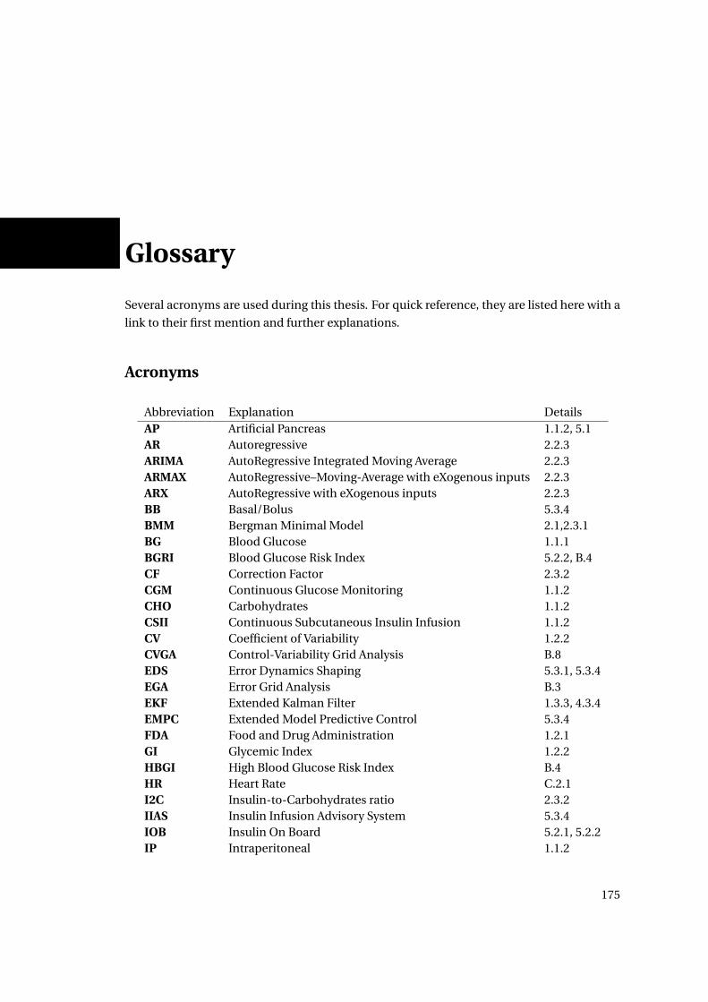
Glossary
Several acronyms are used during this thesis. For quick reference, they are listed here with a
link to their first mention and further explanations.
Acronyms
Abbreviation Explanation DetailsAP Artificial Pancreas 1.1.2, 5.1AR Autoregressive 2.2.3ARIMA AutoRegressive Integrated Moving Average 2.2.3ARMAX AutoRegressive–Moving-Average with eXogenous inputs 2.2.3ARX AutoRegressive with eXogenous inputs 2.2.3BB Basal/Bolus 5.3.4BMM Bergman Minimal Model 2.1,2.3.1BG Blood Glucose 1.1.1BGRI Blood Glucose Risk Index 5.2.2, B.4CF Correction Factor 2.3.2CGM Continuous Glucose Monitoring 1.1.2CHO Carbohydrates 1.1.2CSII Continuous Subcutaneous Insulin Infusion 1.1.2CV Coefficient of Variability 1.2.2CVGA Control-Variability Grid Analysis B.8EDS Error Dynamics Shaping 5.3.1, 5.3.4EGA Error Grid Analysis B.3EKF Extended Kalman Filter 1.3.3, 4.3.4EMPC Extended Model Predictive Control 5.3.4FDA Food and Drug Administration 1.2.1GI Glycemic Index 1.2.2HBGI High Blood Glucose Risk Index B.4HR Heart Rate C.2.1I2C Insulin-to-Carbohydrates ratio 2.3.2IIAS Insulin Infusion Advisory System 5.3.4IOB Insulin On Board 5.2.1, 5.2.2IP Intraperitoneal 1.1.2
175
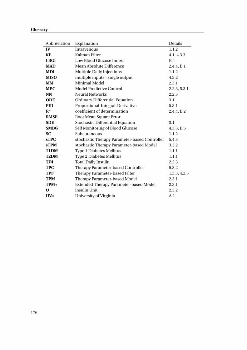
Glossary
Abbreviation Explanation DetailsIV Intravenous 1.1.2KF Kalman Filter 4.1, 4.3.3LBGI Low Blood Glucose Index B.4MAD Mean Absolute Difference 2.4.4, B.1MDI Multiple Daily Injections 1.1.2MISO multiple inputs - single output 4.3.2MM Minimal Model 2.3.1MPC Model Predictive Control 2.2.3, 5.3.1NN Neural Networks 2.2.3ODE Ordinary Differential Equation 3.1PID Proportional-Integral-Derivative 5.3.1R2 coefficient of determination 2.4.4, B.2RMSE Root Mean Square ErrorSDE Stochastic Differential Equation 3.1SMBG Self Monitoring of Blood Glucose 4.3.3, B.5SC Subcutaneous 1.1.2sTPC stochastic Therapy Parameter-based Controller 5.4.3sTPM stochastic Therapy Parameter-based Model 3.3.2T1DM Type 1 Diabetes Mellitus 1.1.1T2DM Type 2 Diabetes Mellitus 1.1.1TDI Total Daily Insulin 2.2.3TPC Therapy Parameter-based Controller 5.3.2TPF Therapy Parameter-based Filter 1.3.3, 4.3.5TPM Therapy Parameter-based Model 2.3.1TPM+ Extended Therapy Parameter-based Model 2.3.1U insulin Unit 2.3.2UVa University of Virginia A.1
176
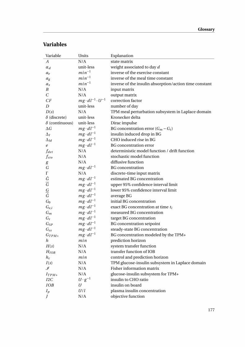
Glossary
Variables
Variable Units ExplanationA N/A state matrixαd unit-less weight associated to day dae mi n−1 inverse of the exercise constantag mi n−1 inverse of the meal time constantax mi n−1 inverse of the insulin absorption/action time constantB N/A input matrixC N/A output matrixC F mg ·dl−1 ·U−1 correction factorD unit-less number of dayD(s) N/A TPM meal perturbation subsystem in Laplace domainδ (discrete) unit-less Kronecker deltaδ (continuous) unit-less Dirac impulse∆G mg ·dl−1 BG concentration error (Gm −Gt )∆I mg ·dl−1 insulin induced drop in BG∆M mg ·dl−1 CHO induced rise in BGe mg ·dl−1 BG concentration errorfdet N/A deterministic model function / drift functionfsto N/A stochastic model functiong N/A diffusive functionG mg ·dl−1 BG concentrationΓ N/A discrete-time input matrixG mg ·dl−1 estimated BG concentrationG mg ·dl−1 upper 95% confidence interval limitG mg ·dl−1 lower 95% confidence interval limitG mg ·dl−1 average BGG0 mg ·dl−1 initial BG concentrationGe,i mg ·dl−1 exact BG concentration at time ti
Gm mg ·dl−1 measured BG concentrationGt mg ·dl−1 target BG concentrationGSP mg ·dl−1 BG concentration setpointGss mg ·dl−1 steady-state BG concentrationGT P M+ mg ·dl−1 BG concentration modeled by the TPM+h mi n prediction horizonH(s) N/A system transfer functionHIOB N/A transfer function of IOBhc mi n control and prediction horizonI (s) N/A TPM glucose-insulin subsystem in Laplace domainI N/A Fisher information matrixIT P M+ N/A glucose-insulin subsystem for TPM+I 2C U · g−1 insulin to CHO ratioIOB U insulin on boardIp U /l plasma insulin concentrationJ N/A objective function
177
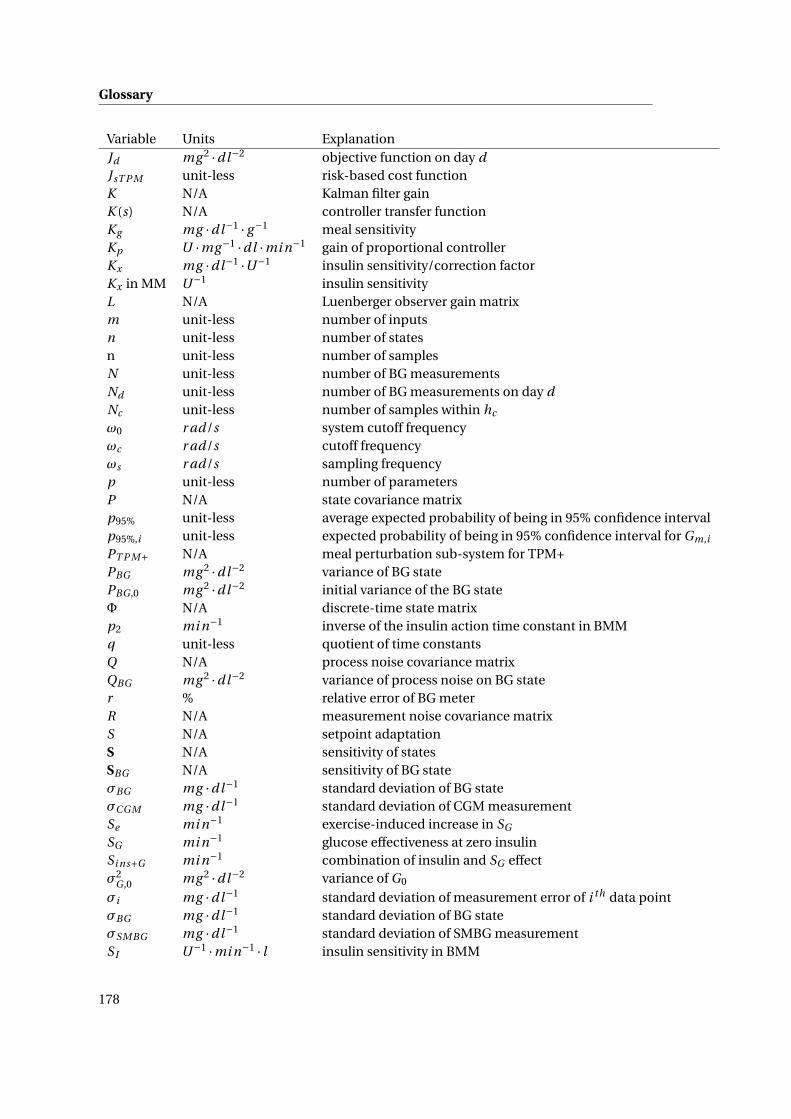
Glossary
Variable Units ExplanationJd mg 2 ·dl−2 objective function on day dJsT P M unit-less risk-based cost functionK N/A Kalman filter gainK (s) N/A controller transfer functionKg mg ·dl−1 · g−1 meal sensitivityKp U ·mg−1 ·dl ·mi n−1 gain of proportional controllerKx mg ·dl−1 ·U−1 insulin sensitivity/correction factorKx in MM U−1 insulin sensitivityL N/A Luenberger observer gain matrixm unit-less number of inputsn unit-less number of statesn unit-less number of samplesN unit-less number of BG measurementsNd unit-less number of BG measurements on day dNc unit-less number of samples within hc
ω0 r ad/s system cutoff frequencyωc r ad/s cutoff frequencyωs r ad/s sampling frequencyp unit-less number of parametersP N/A state covariance matrixp95% unit-less average expected probability of being in 95% confidence intervalp95%,i unit-less expected probability of being in 95% confidence interval for Gm,i
PT P M+ N/A meal perturbation sub-system for TPM+PBG mg 2 ·dl−2 variance of BG statePBG ,0 mg 2 ·dl−2 initial variance of the BG stateΦ N/A discrete-time state matrixp2 mi n−1 inverse of the insulin action time constant in BMMq unit-less quotient of time constantsQ N/A process noise covariance matrixQBG mg 2 ·dl−2 variance of process noise on BG stater % relative error of BG meterR N/A measurement noise covariance matrixS N/A setpoint adaptationS N/A sensitivity of statesSBG N/A sensitivity of BG stateσBG mg ·dl−1 standard deviation of BG stateσCGM mg ·dl−1 standard deviation of CGM measurementSe mi n−1 exercise-induced increase in SG
SG mi n−1 glucose effectiveness at zero insulinSi ns+G mi n−1 combination of insulin and SG effectσ2
G ,0 mg 2 ·dl−2 variance of G0
σi mg ·dl−1 standard deviation of measurement error of i th data pointσBG mg ·dl−1 standard deviation of BG stateσSMBG mg ·dl−1 standard deviation of SMBG measurementS I U−1 ·mi n−1 · l insulin sensitivity in BMM
178
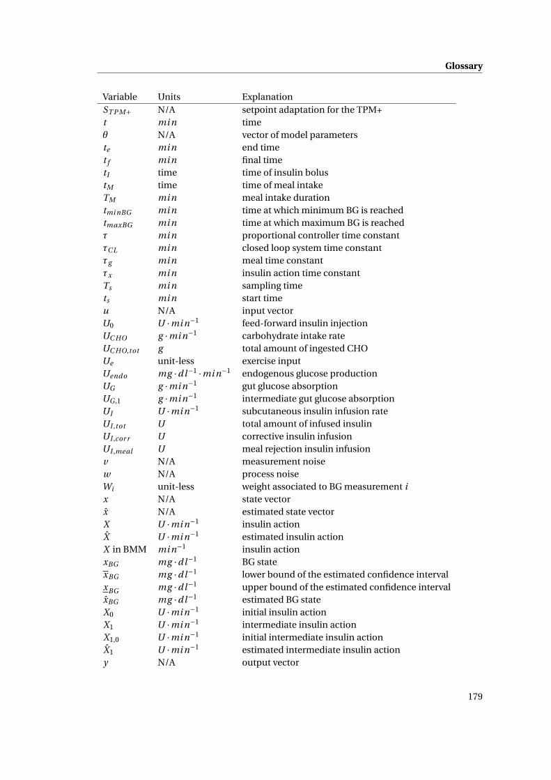
Glossary
Variable Units ExplanationST P M+ N/A setpoint adaptation for the TPM+t mi n timeθ N/A vector of model parameterste mi n end timet f mi n final timetI time time of insulin bolustM time time of meal intakeTM mi n meal intake durationtmi nBG mi n time at which minimum BG is reachedtmaxBG mi n time at which maximum BG is reachedτ mi n proportional controller time constantτC L mi n closed loop system time constantτg mi n meal time constantτx mi n insulin action time constantTs mi n sampling timets mi n start timeu N/A input vectorU0 U ·mi n−1 feed-forward insulin injectionUC HO g ·mi n−1 carbohydrate intake rateUC HO,tot g total amount of ingested CHOUe unit-less exercise inputUendo mg ·dl−1 ·mi n−1 endogenous glucose productionUG g ·mi n−1 gut glucose absorptionUG ,1 g ·mi n−1 intermediate gut glucose absorptionUI U ·mi n−1 subcutaneous insulin infusion rateUI ,tot U total amount of infused insulinUI ,cor r U corrective insulin infusionUI ,meal U meal rejection insulin infusionv N/A measurement noisew N/A process noiseWi unit-less weight associated to BG measurement ix N/A state vectorx N/A estimated state vectorX U ·mi n−1 insulin actionX U ·mi n−1 estimated insulin actionX in BMM mi n−1 insulin actionxBG mg ·dl−1 BG statexBG mg ·dl−1 lower bound of the estimated confidence intervalxBG mg ·dl−1 upper bound of the estimated confidence intervalxBG mg ·dl−1 estimated BG stateX0 U ·mi n−1 initial insulin actionX1 U ·mi n−1 intermediate insulin actionX1,0 U ·mi n−1 initial intermediate insulin actionX1 U ·mi n−1 estimated intermediate insulin actiony N/A output vector
179

Avenue du Tir-Fédéral 79 +41 76 4194760 Luxembourgish (B permit) 1022 Chavannes-près-Renens [email protected] Single Switzerland ch.linkedin.com/in/alainbock 20.06.1985
ALAIN BOCK
EDUCATION PHD IN ELECTRICAL ENGINEERING, Ecole Polytechnique Fédérale de Lausanne 2009 – 01.2014
At the React group and the Laboratoire d’Automatique in collaboration with Roche Diagnostics
MSC IN MECHANICAL ENGINEERING, Ecole Polytechnique Fe de rale de Lausanne 2004 - 2009
Specialized in automatic control and production management
DIPLÔME DE FIN D’ÉTUDES SECONDAIRES, Lycée de Garçons, Luxembourg 1997-2004
Mathematics and physics section
PROJECTS PHD THESIS: MODELS AND MODEL-BASED TOOLS TO IMPROVE TREATMENT OF TYPE 1 DIABETES
Design and validation of a reliable model for predictions of blood glucose concentrations
Development of control method to improve patient safety
Involved in planning and execution of a clinical study to test developed methods
6 months with Roche Diagnostics in Indianapolis, IN, USA
Management of several Master projects
MASTER THESIS: VIBRATION DAMPING CONTROL FOR WIRE ELECTRIC DISCHARGE MACHINING
At the Laboratoire d’Automatique in collaboration with GF AgieCharmilles, Geneva, CH
Modeling and parameter identification of EDM process
Reduction of electrode vibration using complex robust controller design
INTERNSHIPS DESIGN INTERNSHIP, IMAtec, Ettelbruck, Luxembourg 2006
Design of a plastic foil packaging module using CAD software
TOOLING INTERNSHIP, ARCELOR, Differdange, Luxembourg 2005
LANGUAGES ENGLISH, FRENCH, GERMAN: fluent (C2)
SPANISH: basic (A1)
LUXEMBOURGISH: mother tongue
SKILLS TECHNICAL: Optimal control, optimization, parameter identification, population-based methods, data-based
physiological modeling, basic and advanced control methods, stochastic modeling
PROGRAMMING LANGUAGES: Matlab, Simulink, C, C++, Python
SOFTWARE + OS: MS Office, LaTeX, CATIA, Inventor, Windows (XP, Vista, 7, 8), Mac OS X (10.5-8), Android
PUBLICATIONS Bock, A., François, G., & Gillet, D. (2013). A Therapy Parameter-based Model for Predicting Blood
Glucose Concentrations in Patients with Type 1 Diabetes. Comput. Methods Programs Biomed.
Bock, A., François, G., Prud’homme, T., & Gillet, D. (2011). A Minimal Exercise Extension for Models
of the Glucoregulatory System. In Comput. Aided Chem. Eng. (pp. 1520–1524). doi:10.1016/B978-0-
444-54298-4.50083-0
Prud’homme, T., Bock, A., Francois, G., & Gillet, D. (2011). Preclinically assessed optimal control of
postprandial glucose excursions for type 1 patients with diabetes. In 2011 IEEE Int. Conf. Autom.
Sci. Eng. (pp. 702–707). IEEE. doi:10.1109/CASE.2011.6042510
Bock, A., Duke, D. L., & Soni, A. S. (2013). System and Method Considering the
Effect of Physical Activity on the Glucoregulatory System. US 20,130,130,215. 181