Embed Size (px)
Citation preview
Modeling and Characterization of Ammonia Injection and Catalytic Reduction in
Kyrene Unit-7 HRSG
by
Sajesh Adulkar
A Thesis Presented in Partial Fulfillment
of the Requirements for the Degree
Master of Science
Approved November 2011 by the
Graduate Supervisory Committee:
Ramendra Roy, Co-Chair
Taewoo Lee, Co-Chair
Patrick Phelan
ARIZONA STATE UNIVERSITY
May 2012
i
ABSTRACT
The heat recovery steam generator (HRSG) is a key component of
Combined Cycle Power Plants (CCPP). The exhaust (flue gas) from the CCPP gas
turbine flows through the HRSG − this gas typically contains a high concentration
of NO and cannot be discharged directly to the atmosphere because of
environmental restrictions. In the HRSG, one method of reducing the flue gas NO
concentration is to inject ammonia into the gas at a plane upstream of the
Selective Catalytic Reduction (SCR) unit through an injection grid (AIG); the
SCR is where the NO is reduced to N2 and H2O. The amount and spatial
distribution of the injected ammonia are key considerations for NO reduction
while using the minimum possible amount of ammonia.
This work had three objectives. First, a flow network model of the
Ammonia Flow Control Unit (AFCU) was to be developed to calculate the
quantity of ammonia released into the flue gas from each AIG perforation.
Second, CFD simulation of the flue gas flow was to be performed to obtain the
velocity, temperature, and species concentration fields in the gas upstream and
downstream of the SCR. Finally, performance characteristics of the ammonia
injection system were to be evaluated.
All three objectives were reached. The AFCU was modeled using JAVA –
with a graphical user interface provided for the user. The commercial software
Fluent was used for CFD simulation. To evaluate the efficacy of the ammonia
injection system in reducing the flue gas NO concentration, the twelve butterfly

ii
valves in the AFCU ammonia delivery piping (risers) were throttled by various
degrees in the model and the NO concentration distribution computed for each
operational scenario.
When the valves were kept fully open, it was found that it led to a more
uniform reduction in NO concentration compared to throttling the valves such that
the riser flows were equal. Additionally, the SCR catalyst was consumed
somewhat more uniformly, and ammonia slip (ammonia not consumed in
reaction) was found lower. The ammonia use could be decreased by 10 percent
while maintaining the NO concentration limit in the flue gas exhausting into the
atmosphere.

iii
ACKNOWLEDGEMENTS
I am grateful to my advisor, Dr Ramendra Roy, for providing me the
opportunity to work on this research project. I am thankful that Dr. Roy never
accepted less than my best efforts and provided his invaluable advice, guidance,
exceptional support and encouragement throughout the course of my graduate
study and this research work. Salt River Project (SRP) provided funding for this
project. I thank Ivan Insua, engineer at Kyrene Generating Station for being very
helpful in providing the information about the SRP Plants.
I would like to express my gratitude to Dr. Taweoo lee and Dr Patrick
Phelan for consenting to serve as defense committee member.
I am grateful to my lab mates Jagdish, Nihal, Hardeep, Parag and Jayanth
for extending their unfailing help and support through this project.
I owe special thanks to my friends Ashish, Karthik, Robin, and Goutam
for their motivation, support and encouragement. There are many others to whom
I am immensely grateful, all of whose names may not be possible to acknowledge
here personally, nevertheless it may not have been possible to accomplish this
endeavor without them. Thank you.
iv
TABLE OF CONTENTS
Page
LIST OF TABLES………………………………………………………………...x
LIST OF FIGURES……………………………………………………………...xii
CHAPTER
1 INTRODUCTION ...................................................................................... 1
1.1 Heat Recovery Steam Generator in Combined Cycle Power Plant ... 1
1.2 Motivation .......................................................................................... 2
1.3 Scope of work .................................................................................... 3
1.4 Organization of Thesis ....................................................................... 4
2 SRP KYRENE UNIT-7 POWER PLANT ................................................. 5
2.1 Heat Recovery Steam Generator (HRSG) ......................................... 5
2.2 Methodology for solution of velocity, pressure, temperature and
species distribution fields for HRSG ................................................. 7
2.2.1 Velocity and pressure fields simulation for stack ............. 11
2.2.2 Velocity and pressure fields simulation for HRSG
(Modules 1 through 5) ...................................................... 12
2.2.3 Velocity, pressure and temperature fields simulation for
HRSG (Modules 1 & 2) .................................................... 14
v
CHAPTER Page
2.2.4 Velocity, pressure and species concentration fields
simulation for CO-AIG-SCR model ................................. 16
2.3 Ammonia Flow Control Unit (AFCU) ............................................. 18
3 MODELING OF FLOW IN HRSG .......................................................... 22
3.1 Modeling of HRSG internal components ........................................ 22
3.1.1 Perforated plate ................................................................. 22
3.1.2 Duct burner ....................................................................... 24
3.1.3 Tube banks (single-phase flow) ........................................ 24
3.1.3.1 Pressure drop…………………………………...25
3.1.3.2 Heat transfer……………………………………30
3.1.4 Tube banks (two-phase flow)............................................ 39
3.1.4.1 Methodology for single-phase flow in tubes......43
3.1. 4.2 Methodology for two-phase flow in tubes……..44
3.1.4.3 Calculation procedure for two-phase inside heat
transfer coefficient (quality up to 0.8)………... 47
vi
CHAPTER Page
3.1.4.4 Calculation procedure for two-phase inside heat
transfer coefficient (quality above 0.9)……..… 50
3.1.4.5 Calculation procedure for pressure drop inside
tubes (Homogeneous model)…………………. 56
3.1.5 CO Catalyst ....................................................................... 60
3.1.6 Ammonia Injection Grid (AIG) ........................................ 60
3.1.7 SCR Catalyst ..................................................................... 61
3.2 Modeling of Ammonia Flow Control Unit (Java Application) ....... 67
3.2.1 Heat loss from piping and vaporization chamber ............. 68
3.2.2 Pressure drop in piping system ......................................... 72
3.2.3 Vaporization chamber ....................................................... 74
3.2.4 Manifold, Risers and AIG ................................................. 76
3.2.4.1 Orifice plate………………………………....…77
3.2.4.2 Butterfly valve…………………………………78
3.2.4.3 Riser junction…………………….…………….79
3.2.4.4 Manifold junction.……………….…………….80
3.2.4.5 Ammonia Injection Grid (AIG)……….……….83
vii
CHAPTER Page
3.2.4.6 Flow through manifold.……………….……….85
4 THE CFD TOOL ...................................................................................... 91
4.1 Fluent–Introduction.......................................................................... 91
4.2 Reynolds-averaged Navier-Stokes equations .................................. 93
4.3 Turbulence model ............................................................................ 97
4.3.1 The standard k-ε model ..................................................... 97
4.3.2 Near-wall model.............................................................. 102
4.4 Flow solver: ................................................................................... 104
4.4.1 Pressure-based Solver ..................................................... 106
4.5 Cell Zone and Boundary Conditions for computation domain ...... 108
4.5.1 Mass flow boundary conditions at inlet .......................... 109
4.5.2 Pressure boundary condition at outlet ............................. 111
4.5.3 Velocity boundary condition at inlet............................... 111
4.5.4 Radiator boundary condition for pressure drop across
perforated plate, tube banks and catalysts....................... 111
4.5.5 Wall boundary condition for walls ................................. 112
4.5.6 Porous media cell zone condition for catalyst ................ 112
5 RESULTS AND DISCUSSIONS ........................................................... 114
viii
CHAPTER Page
5.1 Flow and temperature simulation results for HRSG ...................... 114
5.1.1 Stack ................................................................................ 114
5.1.2 HRSG (modules 1 through 5) ......................................... 116
5.1.3 HRSG (modules 1 and 2) ................................................ 116
5.2 Flow and species concentration simulation results for CO-AIG-SCR
model.............................................................................................. 123
5.2.1 Case : 1 Equal flow of flue gas+NH3 mixture in all risers
and NH3 at current injection rate .................................... 124
5.2.1.1 Solution for Ammonia flow control model…...124
5.2.1.2 Solution for CO-AIG-SCR model…………....126
5.2.2 Case : 2 Butterfly valves full open and NH3 at current
injection rate.................................................................... 129
5.2.2.1 Solution for Ammonia flow control model…...129
5.2.2.2 Solution for CO-AIG-SCR model……….…...131
5.2.3 Case : 3 Equal flow of flue gas+NH3 mixture in all risers
and NH3 at 90% of current injection rate ....................... 136
5.2.3.1 Solution for Ammonia flow control model…...136
5.2.3.2 Solution for CO-AIG-SCR model……….…...138
ix
CHAPTER Page
5.2.4 Case : 4 Butterfly valves full open and NH3 at 90% of
current injection rate ....................................................... 140
5.2.4.1 Solution for Ammonia flow control model…...140
5.2.4.2 Solution for CO-AIG-SCR model…….……...142
5.2.5 Case : 5 Equal flow of flue gas+NH3 mixture in all risers
and NH3 at 80% of current injection rate………………146
5.2.5.1 Solution for Ammonia flow control model…...146
5.2.5.2 Solution for CO-AIG-SCR model…….……...148
5.2.6 Case : 6 Butterfly valves full open and NH3 at 80% of
current injection rate ....................................................... 150
5.2.6.1 Solution for Ammonia flow control model.…..150
5.2.6.2 Solution for CO-AIG-SCR model……….…...152
5.3 Concluding Remarks ...................................................................... 157
REFERENCES…………………………………………………………………160
x
LIST OF TABLES
Table Page
2.1 Input parameters for velocity and pressure fields simulation ................... 12
2.2 Input parameters for velocity and pressure fields simulation ................... 13
2.3 Input parameters for velocity, pressure and temperature fields simulation
................................................................................................................... 15
2.4 Input parameters for velocity, pressure and species distribution fields
simulation .................................................................................................. 18
2.5 Input parameters for Ammonia Flow Control Unit .................................. 21
3.1 Pressure drop calculation for tube banks with ESCOA method ............... 29
3.2 Sample calculation for one flue gas mass flow rate .................................. 36
3.3 Values of constants for Convective and Nucleate region (Kandlikar) ..... 48
3.4 Two-phase inside heat transfer coefficient for evaporator 1 (row 1) ........ 50
3.5 Two-phase inside heat transfer coefficient for evaporator 2 (row 9) ........ 50
3.6 Two-phase inside heat transfer coefficient for evaporators 1 & 2 ............ 51
3.7 Overall heat transfer coefficient for evaporator 1 (row 1) ........................ 52
3.8 Overall heat transfer coefficient for evaporator 2 (row 9) ........................ 52
3.9 Overall heat transfer coefficient for evaporators (rows 1 through 6) ....... 53
3.10 Overall heat transfer coefficient for evaporators (rows 7 through 12) ..... 54
3.11 Particulars of water / steam for evaporator ............................................... 56
3.12 Pressure drop calculation for evaporator-1 (row 1) .................................. 59
3.13 Pressure drop calculation for evaporator-2 (row 9) .................................. 59
xi
Table Page
3.14 Physical details of SCR Catalyst............................................................... 64
3.15 Porosity calculation ................................................................................... 64
3.16 Surface to Volume ratio calculations ........................................................ 65
3.17 Constants for surface reaction (Ho, Soo, Hoon, In-Sik) ........................... 67
3.18 Details of orifice plate ............................................................................... 77
3.19 Loss coefficient for butterfly valve ........................................................... 79
xii
LIST OF FIGURES
Figure Page
1.1 Schematic diagram of a typical Combined Cycle Power Plant (CCPP) ..... 2
2.1 Side view of HRSG ..................................................................................... 5
2.2 Methodology chart (1 of 2) ......................................................................... 9
2.3 Methodology chart (2 of 2) ....................................................................... 10
2.4 Side view of stack ..................................................................................... 11
2.5 Side view of HRSG (modules 1 through 5) .............................................. 12
2.6 Side view of HRSG (modules 1 and 2) .................................................... 14
2.7 CO-AIG-SCR module ............................................................................... 16
2.8 Schematic diagram of Ammonia Flow Control Unit ................................ 18
2.9 Vaporization chamber ............................................................................... 19
3.1 Pressure loss coefficient for fluid flowing through thick perforated plate
(Idelchik) ................................................................................................... 23
3.2 Modeling of duct burner ........................................................................... 24
3.3 Finned tube bank ....................................................................................... 25
3.4 NTU macro model for finned tube bank ................................................... 31
3.5 Methodology chart to solve for heat transfer through tube bank .............. 32
3.6 Description of NTU macro model ............................................................ 37
3.7 Partial top view of evaporator tubes ......................................................... 40
3.8 Methodology for calculating flue gas temperature downstream of tube row
................................................................................................................... 42
xiii
Figure Page
3.9 Procedure for calculating overall heat transfer coefficient ....................... 44
3.10 Overall heat transfer coefficient for rows 1 through 6 .............................. 55
3.11 Overall heat transfer coefficient for rows 7 through 12 ............................ 55
3.12 CO catalyst ................................................................................................ 60
3.13 Part AIG superimposed on computational cells ........................................ 61
3.14 SCR catalyst .............................................................................................. 63
3.15 Methodology to calculate heat loss rate .................................................... 68
3.16 Cross section of insulated pipe ................................................................. 69
3.17 Piping diagram (3D view) ......................................................................... 72
3.18 Methodology to calculate pressure drop in pipe ....................................... 73
3.19 Schematic diagram for vaporization chamber .......................................... 74
3.20 Single line diagram for manifold and risers .............................................. 76
3.21 Flow coefficient chart (Crane) .................................................................. 77
3.22 Loss coefficient for butterfly valve (Miller) ............................................. 78
3.23 Loss coefficient for riser junction (Bruce, Roland, and Gary) ................. 79
3.24 Pressure head rise in manifold (Bruce, Roland, and Gary) ....................... 80
3.25 Pressure head rise in manifold (Bruce, Roland, and Gary) ....................... 81
3.26 Loss coefficient for manifold junction ...................................................... 83
3.27 Ammonia injection grid ............................................................................ 83
3.28 Methodology to solve flow through manifold .......................................... 85
3.29 Manifold schematic ................................................................................... 87
xiv
Figure Page
3.30 Manifold schematic (For sample calculation) ........................................... 88
4.1 SIMPLE Algorithm ................................................................................. 108
5.1 Pressure (g) contour plots of stack .......................................................... 115
5.2 Velocity vector plot of stack ................................................................... 115
5.3 Velocity vector plot of HRSG (modules 1 through 5) ............................ 116
5.4 Pressure (g) contour plot downstream of module 2 ................................ 117
5.5 Pressure (g) contour plot upstream of module 3 ..................................... 117
5.6 Temperature contour plot of HRSG (modules 1 and 2) .......................... 118
5.7 Streamwise (U) velocity of flue gas downstream of HPSH3 ................. 119
5.8 Temperature of flue gas downstream of HPSH3 .................................... 119
5.9 Temperature of flue gas downstream of Evaporator2 ............................. 120
5.10 Temperature of flue gas upstream and downstream of Evaporators ....... 120
5.11 Steam outlet temperature for evaporator tubes ....................................... 121
5.12 Steam outlet quality for evaporator tubes ............................................... 121
5.13 Streamwise (U) velocity of flue gas downstream of Evaporator 2 ......... 122
5.14 Transverse (V) velocity of flue gas downstream of Evaporator 2 .......... 122
5.15 Static pressure line plot of flue gas at AIG center .................................. 123
5.16 Flue gas - cfm, mass and velocity for case-1 .......................................... 125
5.17 Mass and momentum source terms for case-1 ........................................ 125
5.18 Mole fraction of NH3 for case-1 ............................................................. 126
5.19 Mole fraction of NO for case-1 ............................................................... 126
xv
Figure Page
5.20 NH3 mole fraction at various positions for case-1 ................................. 127
5.21 NO mole fraction at various positions for case-1 ................................... 127
5.22 Flue gas mass flow rate at X=26 m ......................................................... 128
5.23 Temperature and Pressure of flue gas and flue gas + NH3 mixture for
case-2 ...................................................................................................... 130
5.24 Flue gas - cfm, mass and velocity for case-2 .......................................... 130
5.25 Mass and momentum source terms for case-2 ........................................ 131
5.26 Mole fraction of NH3 for case-2 ............................................................. 132
5.27 Mole fraction of NO for case-2 ............................................................... 132
5.28 NH3 mole fraction at various positions for case-2 ................................. 133
5.29 NO mole fraction at various positions for case-2 ................................... 133
5.30 Comparison between case 1 and case 2 – Mass flow rate of NH3 per riser
................................................................................................................. 134
5.31 Comparison between case 1 and case 2 – NH3 mole fraction ................ 135
5.32 Comparison between case 1 and case 2 – NO mole fraction .................. 135
5.33 Flue gas - cfm, mass and velocity for case-3 .......................................... 137
5.34 Mass and momentum source terms for case-3 ........................................ 137
5.35 Mole fraction of NH3 for case-3 ............................................................. 138
5.36 Mole fraction of NO for case-3 ............................................................... 138
5.37 NH3 mole fraction at various positions for case-3 ................................. 139
5.38 NO mole fraction at various positions for case-3 ................................... 139
xvi
Figure Page
5.39 Temperature of flue gas + NH3 mixture at vaporization chamber outlet for
case-4 ...................................................................................................... 141
5.40 Flue gas - cfm, mass and velocity for case-4 .......................................... 141
5.41 Mass and momentum source terms for case-4 ........................................ 142
5.42 Mole fraction of NH3 for case-4 ............................................................. 143
5.43 Mole fraction of NO for case-4 ............................................................... 143
5.44 NH3 mole fraction at various positions in the model for case-4 ............ 144
5.45 NO mole fraction at various positions in the model for case-4 .............. 144
5.46 Comparison between case 3 and case 4 – Mass flow rate of NH3 per riser
................................................................................................................. 145
5.47 Comparison between case 3 and case 4 – NH3 mole fraction ................ 145
5.48 Comparison between case 3 and case 4 – NO mole fraction .................. 146
5.49 Flue gas - cfm, mass and velocity for case-5 .......................................... 147
5.50 Mass and momentum source terms for case-5 ........................................ 147
5.51 Mole fraction of NH3 for case-5 ............................................................. 148
5.52 Mole fraction of NO for case-5 ............................................................... 148
5.53 NH3 mole fraction at various positions for case-5 ................................. 149
5.54 NO mole fraction at various positions for case-5 ................................... 149
5.55 Temperature of flue gas + NH3 mixture at vaporization chamber outlet for
case-6 ...................................................................................................... 151
5.56 Flue gas - cfm, mass and velocity for case-6 .......................................... 151
xvii
Figure Page
5.57 Mass and momentum source terms for case-6 ........................................ 152
5.58 Mole fraction of NH3 for case-6 ............................................................. 153
5.59 Mole fraction of NO for case-6 ............................................................... 153
5.60 NH3 mole fraction at various planes for case-6 ...................................... 154
5.61 NO mole fraction at various planes for case-6 ........................................ 154
5.62 Comparison between case 5 and case 6 – Mass flow rate of NH3 per riser
................................................................................................................. 155
5.63 Comparison between case 5 and case 6 – NH3 mole fraction ................ 156
5.64 Comparison between case 5 and case 6 – NO mole fraction .................. 156

1
CHAPTER 1
INTRODUCTION
1.1 Heat Recovery Steam Generator in Combined Cycle Power Plants
Combined cycle power plants (CCPP) represent one approach for
improving the efficiency of electrical power generation units. It combines Brayton
and Rankine cycles - the power generated by the gas turbine is based on Brayton
cycle whereas that by steam turbine is based on Rankine cycle. The heat recovery
steam generator (HRSG) is a key component of CCPP. The exhaust flue gas from
gas turbine, with its high thermal energy content, is passed through the HRSG.
The transfer of thermal energy from flue gas to water/steam tube banks in the
HRSG generates steam. This steam is then supplied to steam turbine to generate
additional electrical power. The HRSG flue gas is subsequently exhausted to the
atmosphere through a stack. In addition to the water/steam tube banks, the HRSG
also contains Carbon Monoxide (CO) and Selective Catalytic Reduction (SCR)
catalysts for reducing the concentrations of CO and NOx in the flue gas prior to its
exhaust into the atmosphere. A schematic diagram of a typical CCPP is shown in
figure 1.1.
2
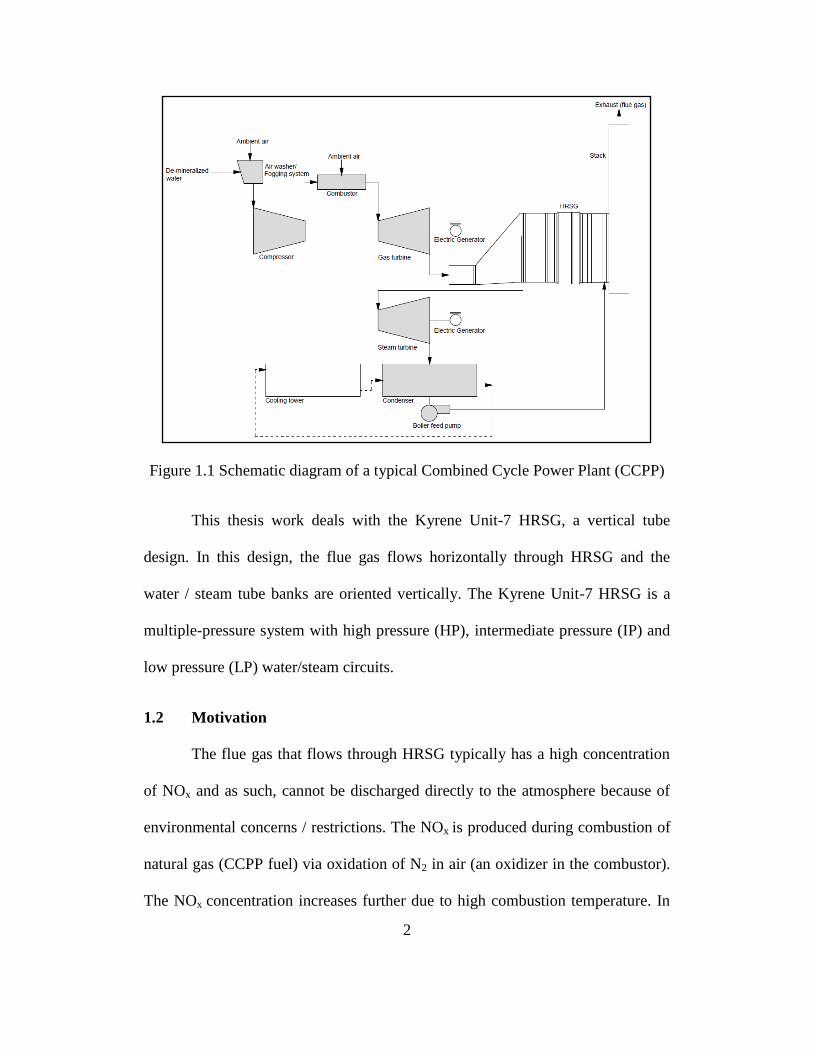
Figure 1.1 Schematic diagram of a typical Combined Cycle Power Plant (CCPP)
This thesis work deals with the Kyrene Unit-7 HRSG, a vertical tube
design. In this design, the flue gas flows horizontally through HRSG and the
water / steam tube banks are oriented vertically. The Kyrene Unit-7 HRSG is a
multiple-pressure system with high pressure (HP), intermediate pressure (IP) and
low pressure (LP) water/steam circuits.
1.2 Motivation
The flue gas that flows through HRSG typically has a high concentration
of NOx and as such, cannot be discharged directly to the atmosphere because of
environmental concerns / restrictions. The NOx is produced during combustion of
natural gas (CCPP fuel) via oxidation of N2 in air (an oxidizer in the combustor).
The NOx concentration increases further due to high combustion temperature. In
3
HRSG, the usual method of reducing the flue gas NOx concentration is to inject
the reducing agent ammonia (NH3) into the gas at a plane upstream of the SCR
catalyst via ammonia injection grid (AIG) - the SCR is where the reduction of
NOx into N2 and H2O takes place. The amount of ammonia injected and the
spatial distribution of this injection in the HRSG are key considerations for
optimum reduction of NOx with the minimum amount of ammonia supplied.
Uniform utilization of the SCR catalyst is an additional consideration.
1.3 Scope of work
This work had three main objectives. Firstly, a flow network model of the
Ammonia Flow Control Unit (AFCU) was to be developed in the form of a Java
based graphic user interface. This flow network model will incorporate all
components of the AFCU and calculates the quantity of ammonia released from
each perforation of the ammonia injection grid (AIG) into HRSG flue gas.
Secondly, computational fluid dynamic (CFD) simulation of the HRSG
gas flow was to be performed to obtain the velocity, pressure, temperature and
species concentration fields in flue gas flow - upstream as well as downstream of
the SCR.
Finally, the performance characteristics of the overall ammonia injection
system were to be evaluated in order to optimize the reduction of NOx in the
HRSG flue gas and minimize the consumption of ammonia.

4
1.4 Organization of Thesis
The thesis work has been described in chapters 2 through 5. Chapter 2
gives an overview of the HRSG, provides detailed insight into methodology used
for the solution of velocity, pressure, temperature and species concentration fields
in the HRSG and a description of the Ammonia Flow Control Unit (AFCU).
Chapter 3 describes the modeling of HRSG components – the perforated
plate, duct burner, tube banks with single-phase steam flow, tube banks with two-
phase steam/water flow, CO catalyst, AIG, and SCR catalyst. It also describes the
modeling of AFCU components – the piping system, vaporization chamber,
manifold, orifice plate, butterfly valves, and AIG.
Chapter 4 gives an overview of the CFD tool, Ansys Fluent, used for
simulation of velocity, pressure, temperature and species concentration fields in
the HRSG. It contains the governing conservation equations, turbulence model
and wall function, pressure-velocity coupling, and the boundary conditions used
to solve the governing equations.
Lastly, chapter 5 provides simulation results for the HRSG components
including the stack and modules 1 through 5. This section also describes the
solution of six simulation cases for CO-AIG-SCR model. A discussion of the
results is provided along with the concluding remarks.
5
CHAPTER 2
SRP KYRENE UNIT-7 POWER PLANT
2.1 Heat Recovery Steam Generator (HRSG)
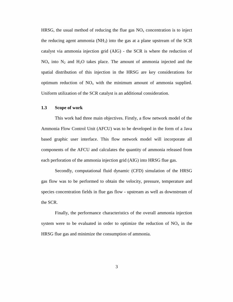
Figure 2.1 Side view of HRSG
The Kyrene unit-7, a CCPP consists of gas turbine and steam turbine,
generating a total of 250 MW of electrical power at full load. The capacity of gas
turbine is 150 MW and that of steam turbine is 100 MW. A triple-pressure HRSG
with vertical tube design is used to generate steam, for steam turbine, by
extracting thermal energy from exhaust flue gas of gas turbine.
The inlet of HRSG is connected to gas turbine outlet. The side view of
HRSG is shown in figure 2.1. The figure also shows the sequence of components
along the flue gas path from inlet to exit of the HRSG. The HRSG consists of
perforated plate, modules 1 through 5 consisting of tube banks, duct burner, CO
catalyst, Ammonia Injection Grid (AIG), SCR catalyst and the stack. The stack is
6
a hollow duct and consists of damper and silencer. The sequence of tube banks
along the flue gas path are as follows:
Module 1
HPSH 1
RHTR 1
In these tube banks the flow of single-phase steam is in positive “Y”
direction.
Module 2
HPSH 2
RHTR 2
HPSH 3
Evaporators 1 & 2
In HPSH 2 and RHTR 2 the flow of single-phase steam is in negative “Y”
direction while it is in positive “Y” direction for HPSH 3. Evaporators 1 & 2 have
two-phase water/steam flow, in positive “Y” direction.
Module 3
IPSH
LPSH
HP Economizer 1
IP Evaporator
Module 4
HP Economizer 2

7
IP Economizer 1
HP Economizer 3
LP Evaporator
Module 5
Feed water heater
As heat transfer analysis for modules 3, 4 and 5 is not carried out, the fluid
flow directions in the tube banks is not noted.
2.2 Methodology for solution of velocity, pressure, temperature and
species distribution fields for HRSG
The CFD simulation procedure and boundary conditions for modeling
HRSG is described in this section. The simulation for HRSG is carried out in four
parts to reduce the computational time. In part one, the solution for velocity and
pressure fields is derived for stack. In part two, the solution for velocity and
pressure fields is derived for HRSG (modules 1 through 5). In part three, the
solution for velocity, pressure and temperature fields is derived for HRSG
(modules 1 and 2). And finally in part four, the solutions for velocity, pressure
and species distribution fields is derived for CO-AIG-SCR model.
The static pressure profile at stack inlet is determined by simulation in part
one is used as outlet boundary condition for HRSG (modules 1 through 5) in part
two. The pressure profile after module 2, from part two, is used as outlet
boundary condition to simulate HRSG (modules 1 and 2). A MatLab code is used
to solve for flue gas temperature downstream of evaporator 2 - a part of module 2.
8
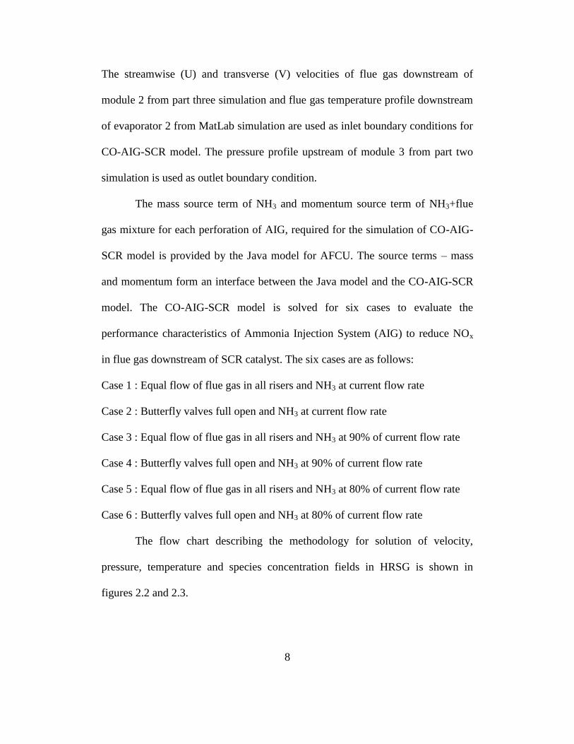
The streamwise (U) and transverse (V) velocities of flue gas downstream of
module 2 from part three simulation and flue gas temperature profile downstream
of evaporator 2 from MatLab simulation are used as inlet boundary conditions for
CO-AIG-SCR model. The pressure profile upstream of module 3 from part two
simulation is used as outlet boundary condition.
The mass source term of NH3 and momentum source term of NH3+flue
gas mixture for each perforation of AIG, required for the simulation of CO-AIG-
SCR model is provided by the Java model for AFCU. The source terms – mass
and momentum form an interface between the Java model and the CO-AIG-SCR
model. The CO-AIG-SCR model is solved for six cases to evaluate the
performance characteristics of Ammonia Injection System (AIG) to reduce NOx
in flue gas downstream of SCR catalyst. The six cases are as follows:
Case 1 : Equal flow of flue gas in all risers and NH3 at current flow rate
Case 2 : Butterfly valves full open and NH3 at current flow rate
Case 3 : Equal flow of flue gas in all risers and NH3 at 90% of current flow rate
Case 4 : Butterfly valves full open and NH3 at 90% of current flow rate
Case 5 : Equal flow of flue gas in all risers and NH3 at 80% of current flow rate
Case 6 : Butterfly valves full open and NH3 at 80% of current flow rate
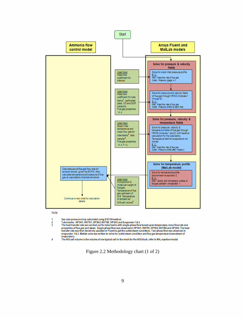
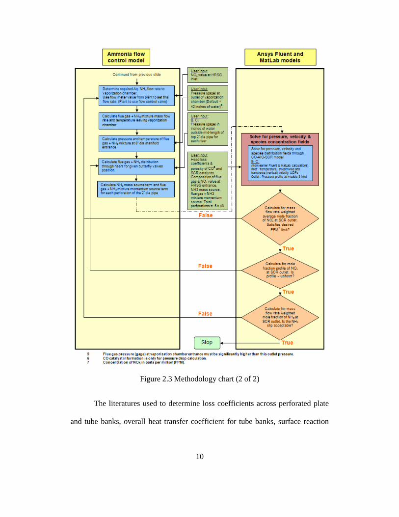
The flow chart describing the methodology for solution of velocity,
pressure, temperature and species concentration fields in HRSG is shown in
figures 2.2 and 2.3.
9
Figure 2.2 Methodology chart (1 of 2)
10
Figure 2.3 Methodology chart (2 of 2)
The literatures used to determine loss coefficients across perforated plate
and tube banks, overall heat transfer coefficient for tube banks, surface reaction
11
for SCR catalyst, modeling vaporization chamber, manifold, AIG etc. are
acknowledged in this thesis work, as and when required at appropriate places.
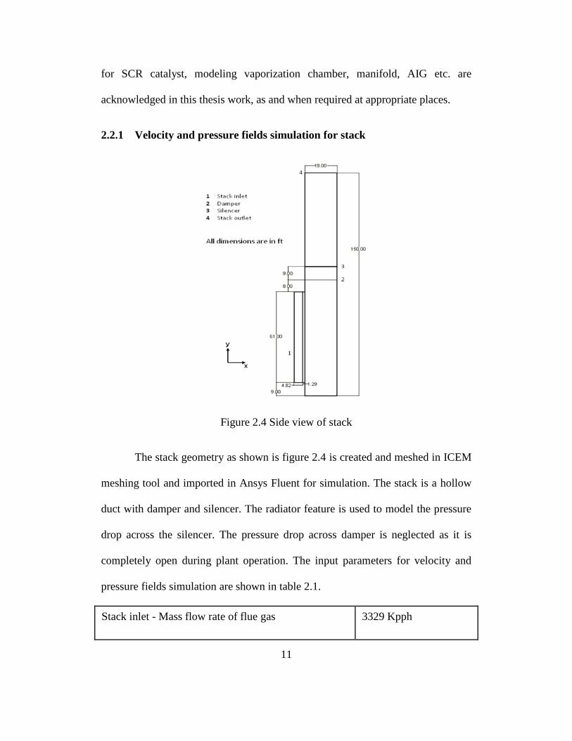
2.2.1 Velocity and pressure fields simulation for stack
Figure 2.4 Side view of stack
The stack geometry as shown is figure 2.4 is created and meshed in ICEM
meshing tool and imported in Ansys Fluent for simulation. The stack is a hollow
duct with damper and silencer. The radiator feature is used to model the pressure
drop across the silencer. The pressure drop across damper is neglected as it is
completely open during plant operation. The input parameters for velocity and
pressure fields simulation are shown in table 2.1.
Stack inlet - Mass flow rate of flue gas 3329 Kpph
12
N2 + Ar (mole % in flue gas) 74.36
O2 (mole % in flue gas) 12.40
CO2 (mole % in flue gas) 03.75
H2O (mole % in flue gas) 09.49
Pressure drop across silencer 1.88 inches of water
Stack outlet - Gage Pressure 0.00 inches of water
Table 2.1 Input parameters for velocity and pressure fields simulation
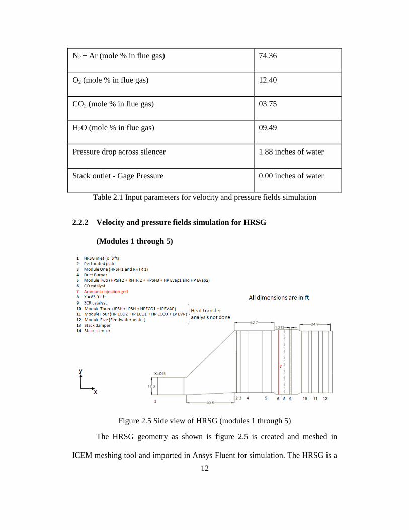
2.2.2 Velocity and pressure fields simulation for HRSG
(Modules 1 through 5)
Figure 2.5 Side view of HRSG (modules 1 through 5)
The HRSG geometry as shown is figure 2.5 is created and meshed in
ICEM meshing tool and imported in Ansys Fluent for simulation. The HRSG is a
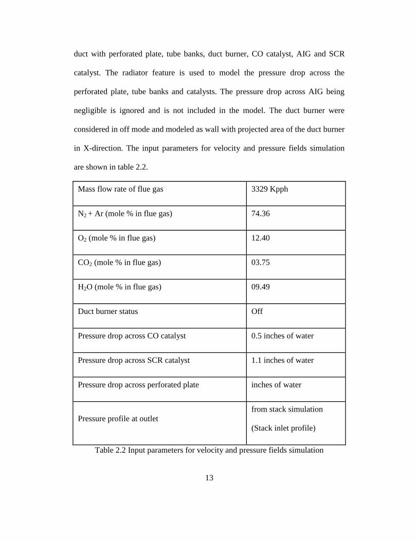
13
duct with perforated plate, tube banks, duct burner, CO catalyst, AIG and SCR
catalyst. The radiator feature is used to model the pressure drop across the
perforated plate, tube banks and catalysts. The pressure drop across AIG being
negligible is ignored and is not included in the model. The duct burner were
considered in off mode and modeled as wall with projected area of the duct burner
in X-direction. The input parameters for velocity and pressure fields simulation
are shown in table 2.2.
Mass flow rate of flue gas 3329 Kpph
N2 + Ar (mole % in flue gas) 74.36
O2 (mole % in flue gas) 12.40
CO2 (mole % in flue gas) 03.75
H2O (mole % in flue gas) 09.49
Duct burner status Off
Pressure drop across CO catalyst 0.5 inches of water
Pressure drop across SCR catalyst 1.1 inches of water
Pressure drop across perforated plate inches of water
Pressure profile at outlet
from stack simulation
(Stack inlet profile)
Table 2.2 Input parameters for velocity and pressure fields simulation
14
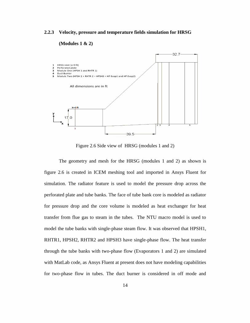
2.2.3 Velocity, pressure and temperature fields simulation for HRSG
(Modules 1 & 2)
Figure 2.6 Side view of HRSG (modules 1 and 2)
The geometry and mesh for the HRSG (modules 1 and 2) as shown is
figure 2.6 is created in ICEM meshing tool and imported in Ansys Fluent for
simulation. The radiator feature is used to model the pressure drop across the
perforated plate and tube banks. The face of tube bank core is modeled as radiator
for pressure drop and the core volume is modeled as heat exchanger for heat
transfer from flue gas to steam in the tubes. The NTU macro model is used to
model the tube banks with single-phase steam flow. It was observed that HPSH1,
RHTR1, HPSH2, RHTR2 and HPSH3 have single-phase flow. The heat transfer
through the tube banks with two-phase flow (Evaporators 1 and 2) are simulated
with MatLab code, as Ansys Fluent at present does not have modeling capabilities
for two-phase flow in tubes. The duct burner is considered in off mode and
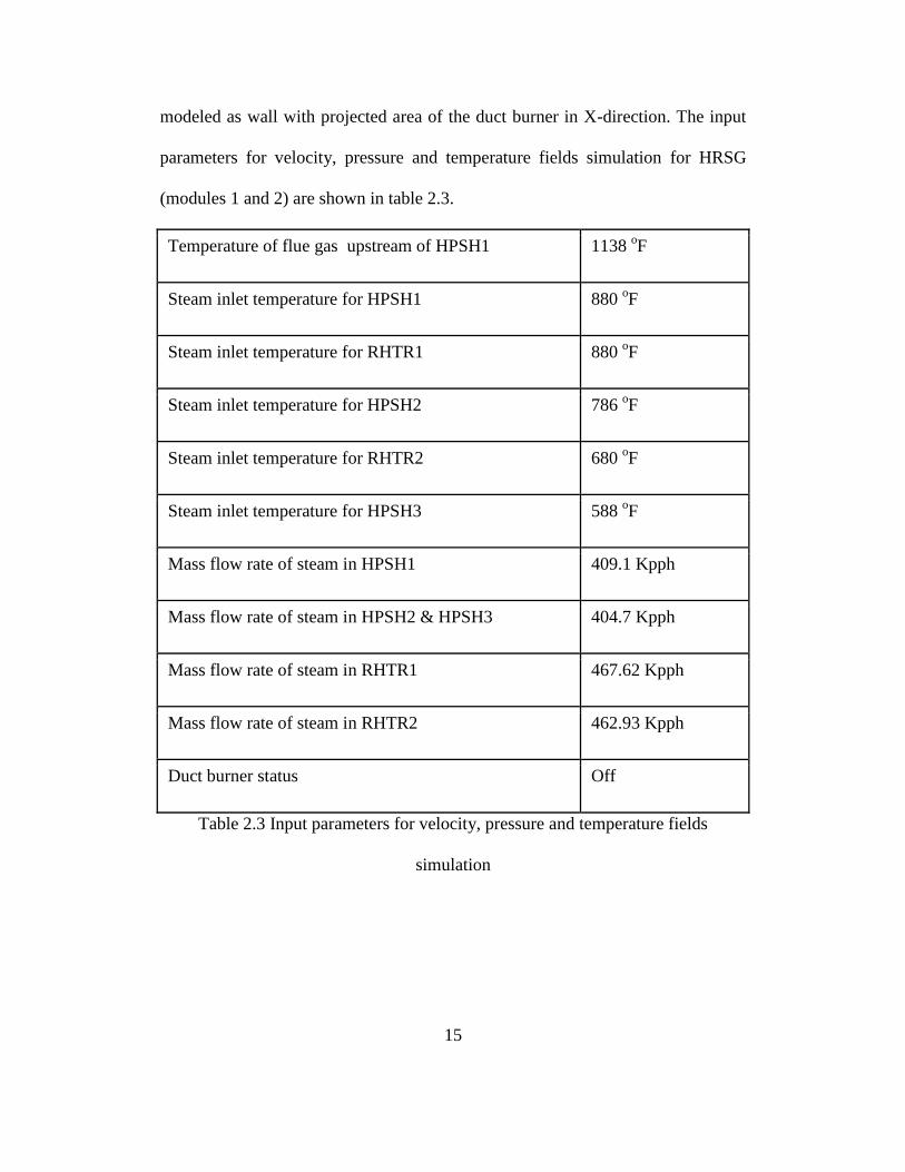
15
modeled as wall with projected area of the duct burner in X-direction. The input
parameters for velocity, pressure and temperature fields simulation for HRSG
(modules 1 and 2) are shown in table 2.3.
Temperature of flue gas upstream of HPSH1 1138 oF
Steam inlet temperature for HPSH1 880 oF
Steam inlet temperature for RHTR1 880 oF
Steam inlet temperature for HPSH2 786 oF
Steam inlet temperature for RHTR2 680 oF
Steam inlet temperature for HPSH3 588 oF
Mass flow rate of steam in HPSH1 409.1 Kpph
Mass flow rate of steam in HPSH2 & HPSH3 404.7 Kpph
Mass flow rate of steam in RHTR1 467.62 Kpph
Mass flow rate of steam in RHTR2 462.93 Kpph
Duct burner status Off
Table 2.3 Input parameters for velocity, pressure and temperature fields
simulation
16
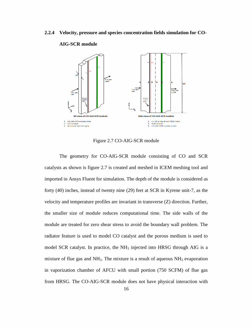
2.2.4 Velocity, pressure and species concentration fields simulation for CO-
AIG-SCR module
Figure 2.7 CO-AIG-SCR module
The geometry for CO-AIG-SCR module consisting of CO and SCR
catalysts as shown is figure 2.7 is created and meshed in ICEM meshing tool and
imported in Ansys Fluent for simulation. The depth of the module is considered as
forty (40) inches, instead of twenty nine (29) feet at SCR in Kyrene unit-7, as the
velocity and temperature profiles are invariant in transverse (Z) direction. Further,
the smaller size of module reduces computational time. The side walls of the
module are treated for zero shear stress to avoid the boundary wall problem. The
radiator feature is used to model CO catalyst and the porous medium is used to
model SCR catalyst. In practice, the NH3 injected into HRSG through AIG is a
mixture of flue gas and NH3. The mixture is a result of aqueous NH3 evaporation
in vaporization chamber of AFCU with small portion (750 SCFM) of flue gas
from HRSG. The CO-AIG-SCR module does not have physical interaction with
17
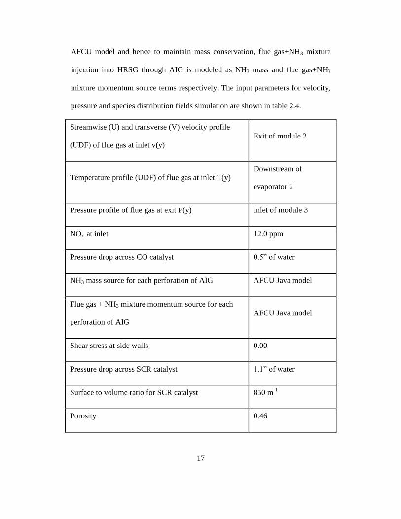
AFCU model and hence to maintain mass conservation, flue gas+NH3 mixture
injection into HRSG through AIG is modeled as NH3 mass and flue gas+NH3
mixture momentum source terms respectively. The input parameters for velocity,
pressure and species distribution fields simulation are shown in table 2.4.
Streamwise (U) and transverse (V) velocity profile
(UDF) of flue gas at inlet v(y)
Exit of module 2
Temperature profile (UDF) of flue gas at inlet T(y)
Downstream of
evaporator 2
Pressure profile of flue gas at exit P(y) Inlet of module 3
NOx at inlet 12.0 ppm
Pressure drop across CO catalyst 0.5” of water
NH3 mass source for each perforation of AIG AFCU Java model
Flue gas + NH3 mixture momentum source for each
perforation of AIG
AFCU Java model
Shear stress at side walls 0.00
Pressure drop across SCR catalyst 1.1” of water
Surface to volume ratio for SCR catalyst 850 m-1
Porosity 0.46
18
Pre-exponential factor ANO 3.51 m/sec
Pre-exponential factor ANH3 6.91 e-5 m3/mole
Activation energy for NO reduction 14.2 Kcal/mole
Change in enthalpy for NH3 equilibrium 22.2 Kcal/mole
Table 2.4 Input parameters for velocity, pressure and species distribution fields
simulation
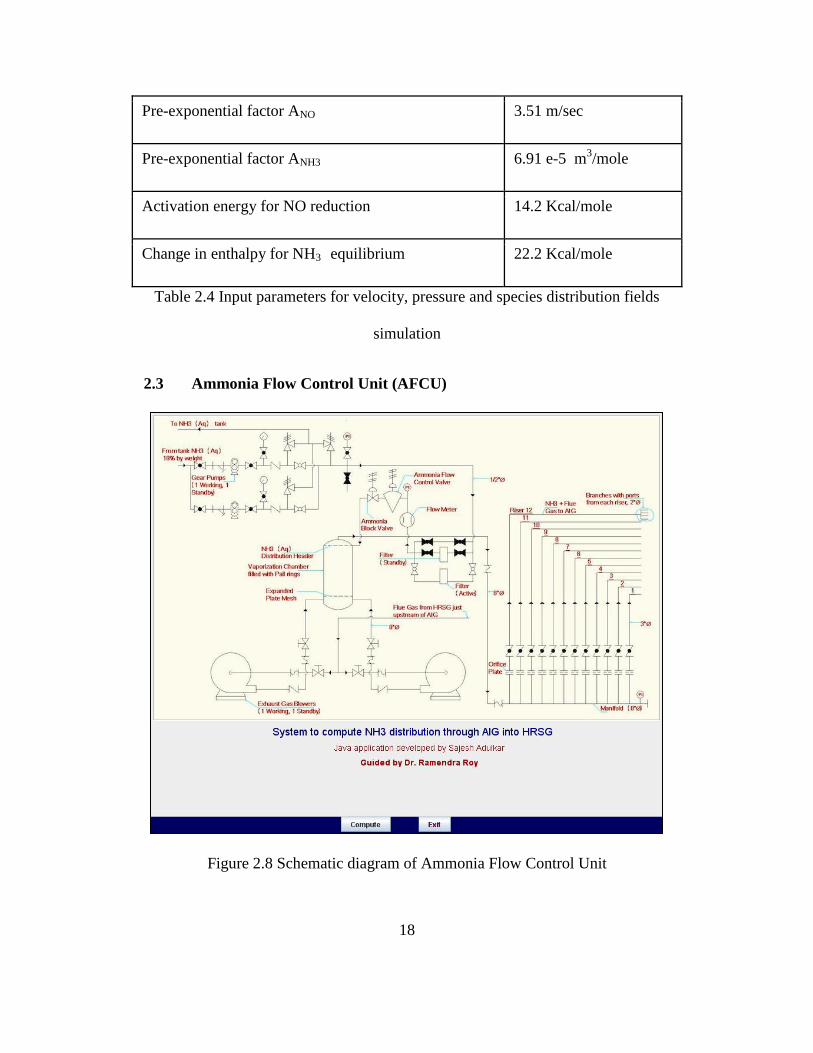
2.3 Ammonia Flow Control Unit (AFCU)
Figure 2.8 Schematic diagram of Ammonia Flow Control Unit
19
The AFCU as shown is figure 2.8 consists of aqueous ammonia discharge
pumps (1 working, 1 standby). The aqueous ammonia (19% by weight) is pumped
from storage tank to vaporization chamber through flow meter and ammonia flow
control valve. The ammonia flow control valve controls the flow of aqueous
ammonia into vaporization chamber. There is a flow meter before the control
valve to measure the consumption of aqueous ammonia and a block valve after
control valve to isolate the control valve for maintenance. The aqueous ammonia
is pumped through a line of ½” un-insulated steel pipe. The pneumatic ammonia
flow control valve operates on many input parameters; however the important
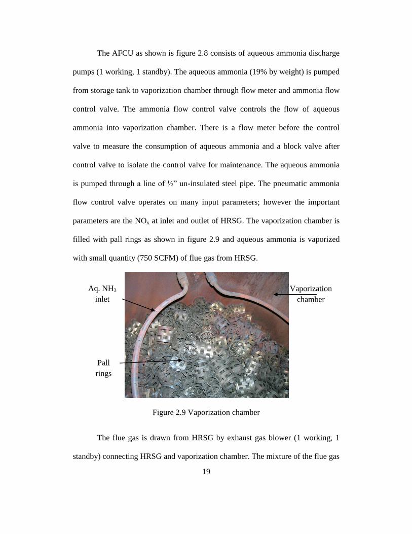
parameters are the NOx at inlet and outlet of HRSG. The vaporization chamber is
filled with pall rings as shown in figure 2.9 and aqueous ammonia is vaporized
with small quantity (750 SCFM) of flue gas from HRSG.
Figure 2.9 Vaporization chamber
The flue gas is drawn from HRSG by exhaust gas blower (1 working, 1
standby) connecting HRSG and vaporization chamber. The mixture of the flue gas
Vaporization
chamber
Pall
rings
Aq. NH3
inlet
20
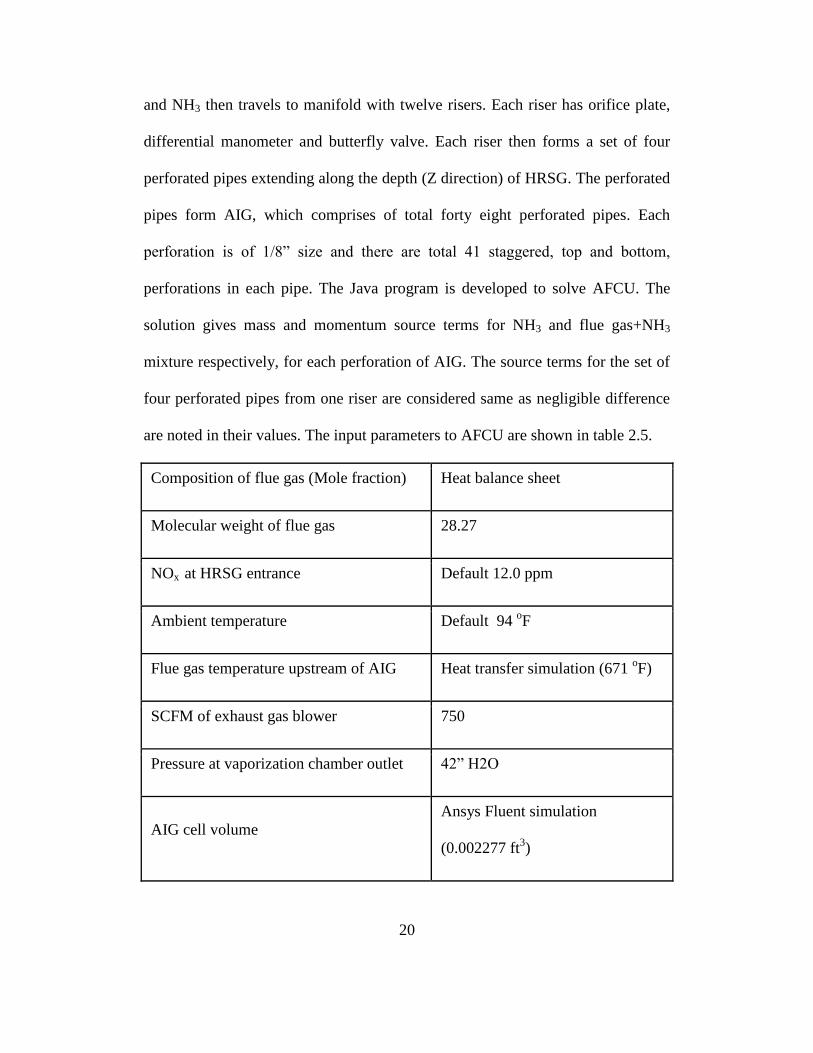
and NH3 then travels to manifold with twelve risers. Each riser has orifice plate,
differential manometer and butterfly valve. Each riser then forms a set of four
perforated pipes extending along the depth (Z direction) of HRSG. The perforated
pipes form AIG, which comprises of total forty eight perforated pipes. Each
perforation is of 1/8” size and there are total 41 staggered, top and bottom,
perforations in each pipe. The Java program is developed to solve AFCU. The
solution gives mass and momentum source terms for NH3 and flue gas+NH3
mixture respectively, for each perforation of AIG. The source terms for the set of
four perforated pipes from one riser are considered same as negligible difference
are noted in their values. The input parameters to AFCU are shown in table 2.5.
Composition of flue gas (Mole fraction) Heat balance sheet
Molecular weight of flue gas 28.27
NOx at HRSG entrance Default 12.0 ppm
Ambient temperature Default 94 oF
Flue gas temperature upstream of AIG Heat transfer simulation (671 oF)
SCFM of exhaust gas blower 750
Pressure at vaporization chamber outlet 42” H2O
AIG cell volume
Ansys Fluent simulation
(0.002277 ft3)

21
Pressure in HRSG at AIG ports discharge
(inches of H2O)
Ansys Fluent simulation
Butterfly valve opening
As required to minimize mass-
weighted average of NOx at SCR
downstream
Table 2.5 Input parameters for Ammonia Flow Control Unit
22
CHAPTER 3
MODELING OF FLOW IN HRSG
3.1 Modeling of HRSG internal components
The HRSG consists of perforated plate, tube banks, duct burner, CO and
SCR catalysts. There is a pressure drop through each of these components, heat
transfer in tube banks (considered up to module 2) and surface reaction in SCR
catalyst. All the components are modeled in Ansys Fluent except for heat transfer
in evaporators, where two-phase flow is observed and is modeled in MatLab. The
modeling of all the components has been covered in this chapter.
3.1.1 Perforated plate
The perforated plate is considered as thick plate as the ratio of plate
thickness (l) and perforation diameter is greater than 0.015 (l/dh≥0.015). The loss
coefficient of perforated plate depends on free area coefficient, the shape of
perforation edge and Reynolds number of flue gas upstream of perforated plate.
The free area coefficient is defined as follows:
(1)
where, : Free area coefficient, Fo : Net free area of perforated plate and F : Area
of perforated plate.
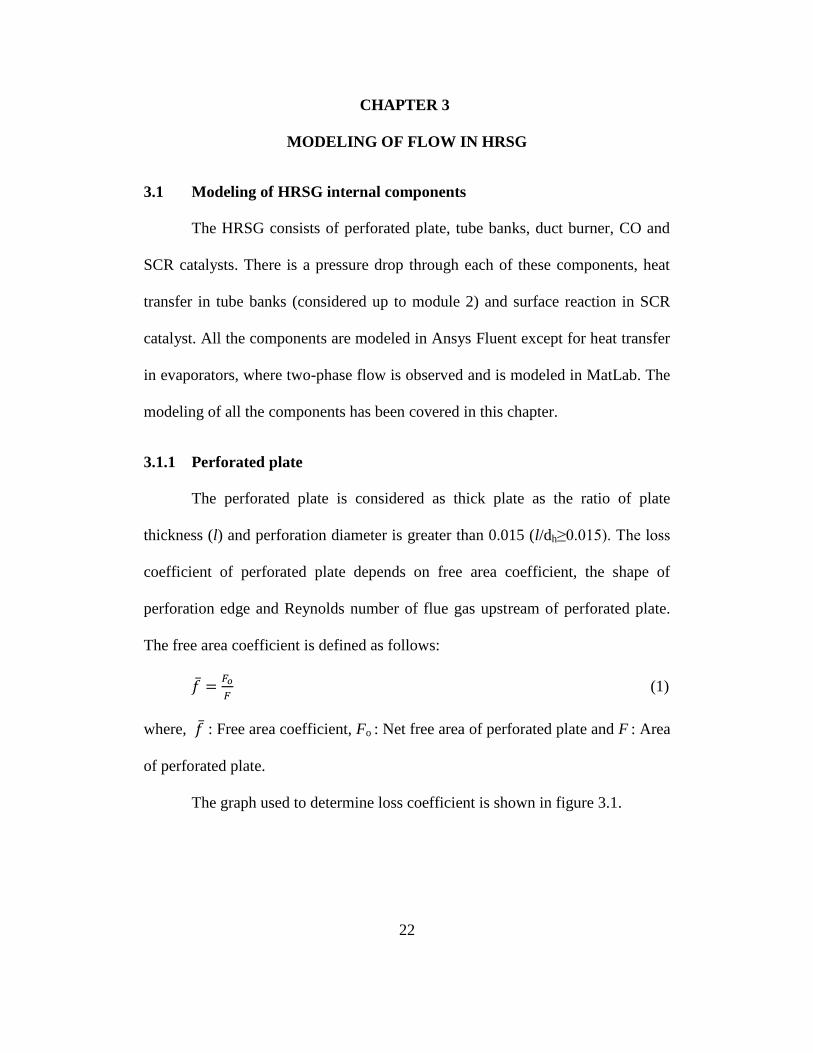
The graph used to determine loss coefficient is shown in figure 3.1.
23
Figure 3.1 Pressure loss coefficient for fluid flowing through thick perforated
plate (Idelchik)
The pressure drop across the perforated plate is subsequently worked out
as follows:
(2)
The radiator feature is used to model the pressure drop across perforated
plate in the CFD model. The loss coefficient to model the pressure drop is worked
out as follows:
(3)
where, : Loss coefficient, : Density of flue gas, : Streamwise velocity of
flue gas upstream of perforated plate and : Pressure drop across perforated
plate
24
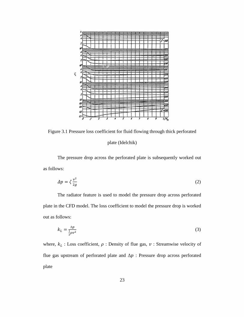
3.1.2 Duct burner
The duct burner is considered in off mode and modeled as wall with the
projected area of duct burner in X-direction. The actual configuration and Fluent
model for the duct burner is shown in figure 3.2.
Figure 3.2 Modeling of duct burner
3.1.3 Tube banks (single-phase flow)
The flue gas experiences pressure and temperature drop across the tube
banks. The modeling of pressure drop and heat transfer for tube banks with
single-phase flow is explained in section 3.1.3.1 and 3.1.3.2 respectively.
25
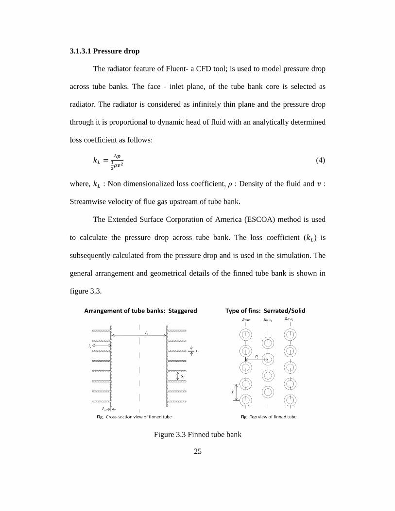
3.1.3.1 Pressure drop
The radiator feature of Fluent- a CFD tool; is used to model pressure drop
across tube banks. The face - inlet plane, of the tube bank core is selected as
radiator. The radiator is considered as infinitely thin plane and the pressure drop
through it is proportional to dynamic head of fluid with an analytically determined
loss coefficient as follows:
(4)
where, : Non dimensionalized loss coefficient, ρ : Density of the fluid and :
Streamwise velocity of flue gas upstream of tube bank.
The Extended Surface Corporation of America (ESCOA) method is used
to calculate the pressure drop across tube bank. The loss coefficient ( ) is
subsequently calculated from the pressure drop and is used in the simulation. The
general arrangement and geometrical details of the finned tube bank is shown in
figure 3.3.
Figure 3.3 Finned tube bank
26
The ESCOA method requires physical data of tube bank such as type of
external tube fins, number of rows, transverse pitch, longitudinal pitch, tube
outside diameter, fin height, number of fins per inch and fin thickness (Martinez,
Vicente, Salinas, and Soto).
The HRSG cross section, temperature and mass flow rate of flue gas
upstream of each tube bank is also recorded. The flue gas mass velocity is then
calculated as follows:
(5)
(6)
The pressure drop across tube bank is calculated as follows:
(7)
where, C2, C4, and C6 are factors and are calculated with the help of Weierman
correlations.
Reynolds correction factor, C2
(8)
Geometry correction factor, C4
For staggered pattern,
(Serrated fins) (9)
(Solid fins) (10)
27
Non-equilateral & row correction factor, C6
(11)
where, Reynolds number and factor “a” are calculated as follows:
(12)
(13)
where,
Nr: Number of tube rows Gn: Mass flue gas velocity (lb/hr/ft2)
m: Mass flue gas flow rate (lb/hr) tw: Tube thickness
pt: Transverse pitch Ac: Cross sectional area of HRSG
sf: Fin spacing f/in: Fins / inch
ld: Tube inner diameter Amin: Net free area for flue gas
do: Tube outer diameter Re: Reynolds number
pl: Longitudinal pitch av: Bulk flue gas density
tf: Fin thickness µb: Bulk viscosity
fd: Fin diameter lf : Fin height
in: Flue gas density before tube bank and out: Flue gas density after tube bank
Once the pressure drop is calculated the loss coefficient is worked out
using equation (4). The isothermal simulation for velocity and pressure fields of
HRSG (modules 1 through 5) is carried out for the flue gas temperature of 1138
28
oF i.e. the temperature of flue gas at HRSG inlet. The loss coefficient is updated
for simulation using a density ratio as follows:
(14)
where, : Loss coefficient at 1138 oF, ρ2 : Density of the flue gas at 1138
oF,
: Loss coefficient at flue gas temperature before tube bank and ρ1 : Density of
the flue gas at flue gas temperature before tube bank.
29
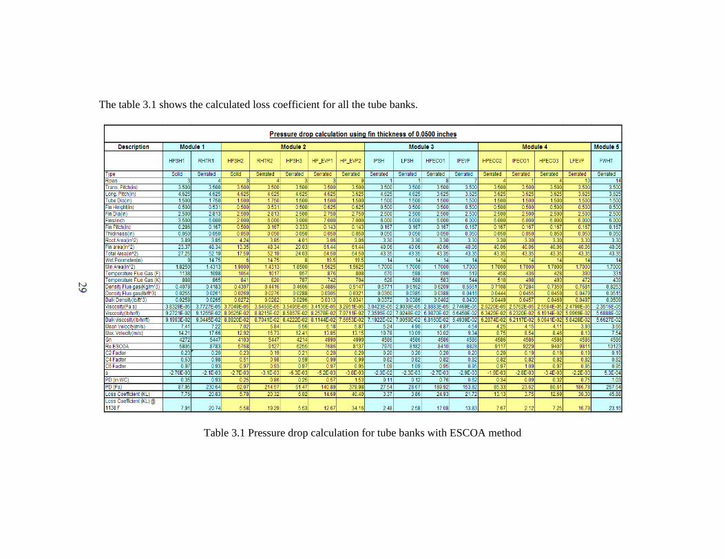
The table 3.1 shows the calculated loss coefficient for all the tube banks.
Table 3.1 Pressure drop calculation for tube banks with ESCOA method

30
3.1.3.2 Heat transfer
In HRSG, the flue gas has to pass through two modules with total seven
tube banks before reaching SCR catalyst. The heat transfer from flue gas to these
tube banks needs to be modeled for velocity and temperature profiles of flue gas,
upstream of SCR catalyst. It is noted that the first five tube banks has single-phase
flow and the last two tube banks has two-phase flow. The tube banks with single-
phase flow are HPSH1, RHTR1, HPSH2, RHTR2 and HPSH3 whereas tube
banks with two-phase flow are evaporators 1 and 2. The procedure to calculate
inside heat transfer coefficient for tube bank with single-phase flow is different
than for tube bank with two-phase flow. The heat transfer for the single-phase
tube banks are modeled in Fluent with NTU macro model whereas the heat
transfer for two-phase tube banks are modeled by writing a code in MatLab.
The NTU macro model is used to simulate heat transfer through the tube
bank, since it is suitable for flow with strong variation in the primary fluid
velocity profile. The fluid within the tubes is referred to as auxiliary fluid and
fluid outside the tubes is referred to as primary fluid. The core of the tube bank
(Heat Exchanger-HX) is treated as fluid zone and is sized to its physical
dimensions. The heat transfer is modeled as heat source in the energy equation.
The model is specifically suitable for compact heat exchanger having single or
multiple auxiliary fluid paths and single unidirectional primary fluid flow. The
core of the tube bank is subdivided into macroscopic cells called macros along the
auxiliary fluid path. The core is subdivided since the heat rejection is not constant
31
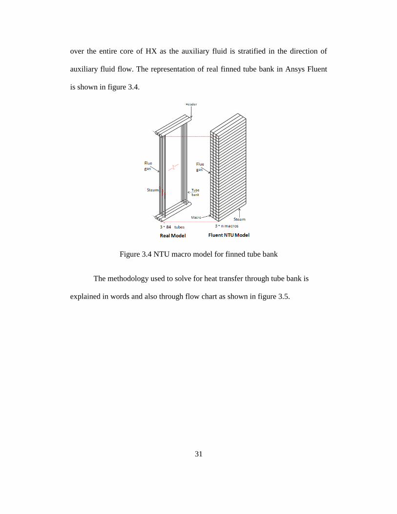
over the entire core of HX as the auxiliary fluid is stratified in the direction of
auxiliary fluid flow. The representation of real finned tube bank in Ansys Fluent
is shown in figure 3.4.
Figure 3.4 NTU macro model for finned tube bank
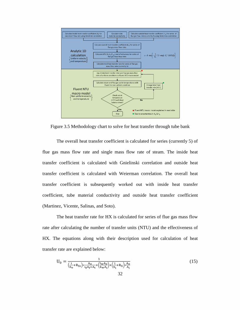
The methodology used to solve for heat transfer through tube bank is
explained in words and also through flow chart as shown in figure 3.5.
32
Figure 3.5 Methodology chart to solve for heat transfer through tube bank
The overall heat transfer coefficient is calculated for series (currently 5) of
flue gas mass flow rate and single mass flow rate of steam. The inside heat
transfer coefficient is calculated with Gnielinski correlation and outside heat
transfer coefficient is calculated with Weierman correlation. The overall heat
transfer coefficient is subsequently worked out with inside heat transfer
coefficient, tube material conductivity and outside heat transfer coefficient
(Martinez, Vicente, Salinas, and Soto).
The heat transfer rate for HX is calculated for series of flue gas mass flow
rate after calculating the number of transfer units (NTU) and the effectiveness of
HX. The equations along with their description used for calculation of heat
transfer rate are explained below:
(15)
33
where,
Uo = Overall heat transfer coefficient ho = Outside heat transfer coefficient
Rfo = Outside fouling factor ηf = Fin efficiency
Af = Fin surface area At = Bare tube surface area
tw = Tube wall thickness Ao = Total outside surface area
Kw = Tube wall thermal conductivity Ai = Inside tube surface area
hi = Inside film heat transfer coefficient Rfi = Inside fouling resistance
The thermal conductivity of tube material - T91 is calculated with
equation 16 (Ashrafi-Nik).
(16)
The inside heat transfer coefficient is calculated using Gnielinski
correlation as follows:
(17)
(18)
(19)
where,
k = Av. thermal conductivity of the steam hi = Inside heat transfer coefficient
di = Inside tube diameter Pr = Av. Prandlt number for steam
Gn = Mass flow rate per ft2
μ = Av. dynamic viscosity of steam
Re = Reynolds number f = Friction factor
34
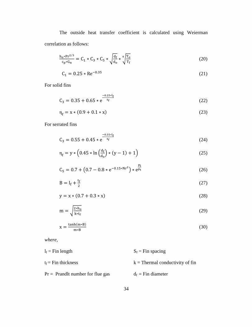
The outside heat transfer coefficient is calculated using Weierman
correlation as follows:
(20)
(21)
For solid fins
(22)
(23)
For serrated fins
(24)
(25)
(26)
(27)
(28)
(29)
(30)
where,
lf = Fin length Sf = Fin spacing
tf = Fin thickness k = Thermal conductivity of fin
Pr = Prandlt number for flue gas df = Fin diameter
35
do = Tube outside diameter di = Tube inside diameter
To = Flue gas temperature Tf = Average fin temperature
C1, C3 and C5 are determined using Weierman Correlation
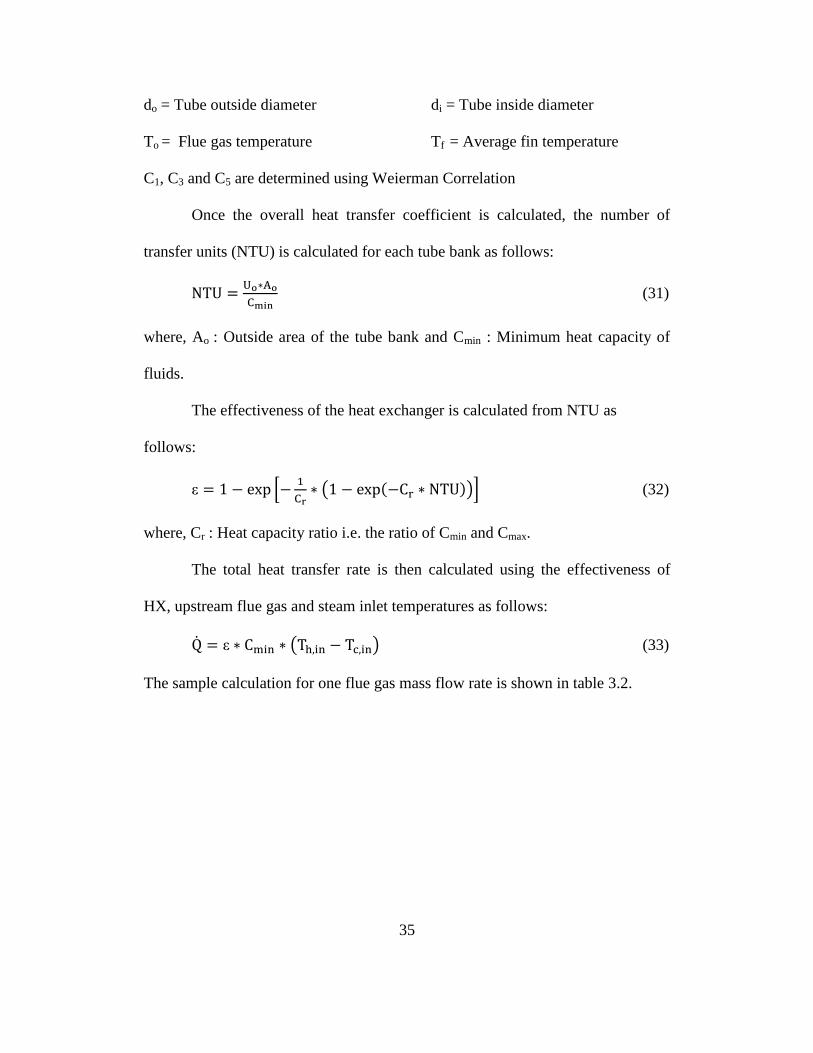
Once the overall heat transfer coefficient is calculated, the number of
transfer units (NTU) is calculated for each tube bank as follows:
(31)
where, Ao : Outside area of the tube bank and Cmin : Minimum heat capacity of
fluids.
The effectiveness of the heat exchanger is calculated from NTU as
follows:
ε
(32)
where, Cr : Heat capacity ratio i.e. the ratio of Cmin and Cmax.
The total heat transfer rate is then calculated using the effectiveness of
HX, upstream flue gas and steam inlet temperatures as follows:
ε (33)
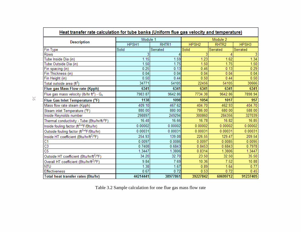
The sample calculation for one flue gas mass flow rate is shown in table 3.2.
36
Table 3.2 Sample calculation for one flue gas mass flow rate
37
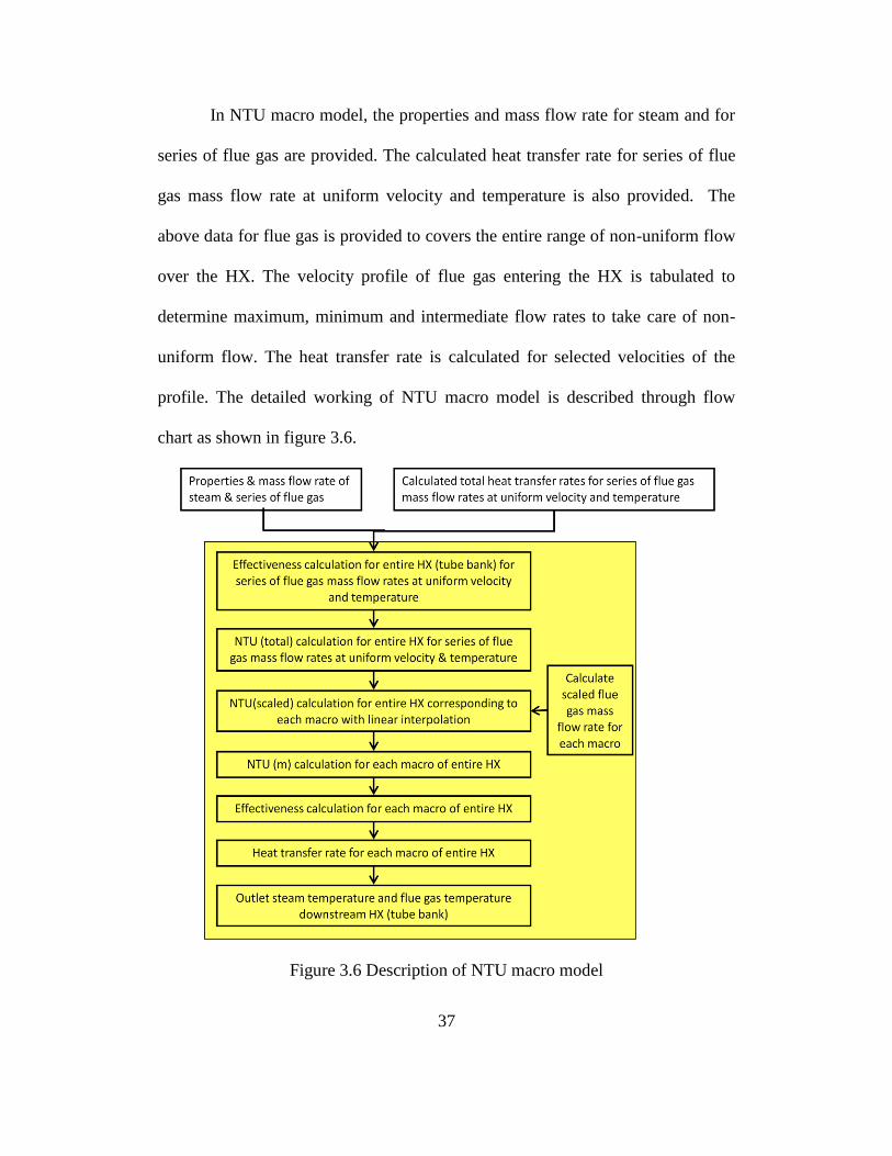
In NTU macro model, the properties and mass flow rate for steam and for
series of flue gas are provided. The calculated heat transfer rate for series of flue
gas mass flow rate at uniform velocity and temperature is also provided. The
above data for flue gas is provided to covers the entire range of non-uniform flow
over the HX. The velocity profile of flue gas entering the HX is tabulated to
determine maximum, minimum and intermediate flow rates to take care of non-
uniform flow. The heat transfer rate is calculated for selected velocities of the
profile. The detailed working of NTU macro model is described through flow
chart as shown in figure 3.6.
Figure 3.6 Description of NTU macro model
38
The effectiveness of entire HX core is computed for series of flue gas
mass flow rate and single steam flow rate from the properties of flue gas and
steam and heat transfer rates using equation 32.
The table of NTU (total) for series of mass flow rate of flue gas is
generated for uniform velocity and temperature as follows:
ε
(34)
The NTU (scaled) is then calculated for each macro of the HX using
scaled flue gas mass flow rate. The NTU macro (m) for each macro is then
calculated from NTU (scaled). The equations for calculating NTU macro (m) are
proprietary and hence not recorded in this thesis document. The effectiveness and
heat transfer rate for each macro are determined with equations 32 and 33
respectively (Ansys).
Once the heat transfer rate is worked out the flue gas temperature
downstream of HX and steam temperature at the outlet of each macro is
determined as follows:
(35)
The total heat transfer rate for the HX is the sum of heat transfer rate of all
the macros comprising the HX. The downstream temperature of flue gas is
compared with the temperature in heat balance sheet. The total heat transfer rates
(all five) are changed to get the temperature within ±2 oF. As the exact
geometrical details of the tube banks are not known the heat transfer rates are
39
changed manually to get the temperature in the range of ±2 oF that of heat balance
sheet.
3.1.4 Tube banks (two-phase flow)
The evaporators 1 and 2 have two-phase flow and comprises of 12 rows of
tubes. The evaporator-1 is comprised of first three rows and evaporator-2 is
comprised of last nine rows. The tube size of evaporator-1 and evaporator-2 is
same however they have different longitudinal pitch. The pressure drop in the
tube is checked using homogeneous model.
The overall heat transfer coefficient is calculated with equation 15. The
outside heat transfer coefficient is calculated with Weierman‟s correlation
(equation 19) and the inside heat transfer coefficient is calculated with
Kandlikar‟s correlation (up to the quality of 0.8) and Groeneveld‟s correlation
(from quality 0.9 to 1.0). Linear interpolation is carried out to calculate inside heat
transfer coefficient for steam quality from 0.8 to 0.9.
The inside heat transfer coefficient for single-phase flow observed in the
lower part of all the tubes and top part of some of the tubes is calculated with
Gnielinski correlation as explained earlier in section 3.1.3.2. The partial top view
of evaporator tubes is shown in figure 3.7.
40
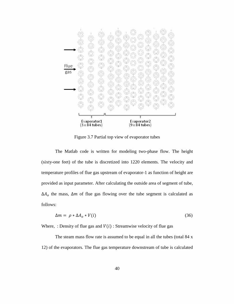
Figure 3.7 Partial top view of evaporator tubes
The Matlab code is written for modeling two-phase flow. The height
(sixty-one feet) of the tube is discretized into 1220 elements. The velocity and
temperature profiles of flue gas upstream of evaporator-1 as function of height are
provided as input parameter. After calculating the outside area of segment of tube,
the mass, of flue gas flowing over the tube segment is calculated as
follows:
(36)
Where, : Density of flue gas and : Streamwise velocity of flue gas
The steam mass flow rate is assumed to be equal in all the tubes (total 84 x
12) of the evaporators. The flue gas temperature downstream of tube is calculated

41
for only one tube row as the flue gas velocity and temperature profiles are
invariant in transverse (Z) direction.
The fluid entering the tubes is sub-cooled water having quality zero. The
methodology flow chart explaining the procedure used to calculate the flue gas
temperature downstream of tube row and exit steam temperature and quality for
each tube row is shown in figure 3.8.
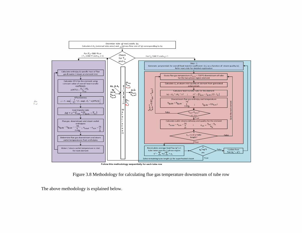
42
Figure 3.8 Methodology for calculating flue gas temperature downstream of tube row
The above methodology is explained below.
43
3.1.4.1 Methodology for single-phase flow in tubes
The enthalpies and specific heats of flue gas and water / steam as function
of temperature are provided as input parameter. The NTU for lower most element
of the tube is calculated as follows:
(37)
where, : Overall heat transfer coefficient and : Minimum heat capacity of
fluid
The Uo is worked out using equation 15. The inside and outside heat
transfer coefficients required for calculating Uo are worked out using equations 17
and 20 respectively. The effectiveness is calculated as function of NTU and after
that the heat transfer rate for the tube segment is calculated as follows:
ε
(38)
ε (39)
where : Heat capacity ratio
The enthalpies of flue gas downstream of element and water / steam
coming out from each element are worked out as follows:
(40)
(41)
The temperature is subsequently calculated as function of enthalpy. The
above loop is repeated for the subsequent tube elements till the saturation
temperature of the water is reached. The same above methodology is also used for
44
steam (quality one and for temperature equal to saturation temperature and above)
found in the upper portion of some of the tube bank until the height of the tube.
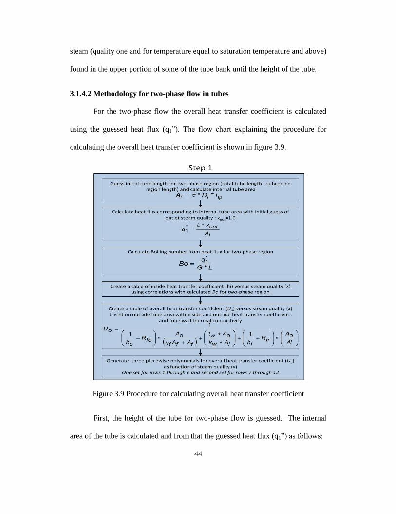
3.1.4.2 Methodology for two-phase flow in tubes
For the two-phase flow the overall heat transfer coefficient is calculated
using the guessed heat flux (q1”). The flow chart explaining the procedure for
calculating the overall heat transfer coefficient is shown in figure 3.9.
Figure 3.9 Procedure for calculating overall heat transfer coefficient
First, the height of the tube for two-phase flow is guessed. The internal
area of the tube is calculated and from that the guessed heat flux (q1”) as follows:
45
(42)
(43)
The boiling number is than calculated as follows:
(44)
where, G : mass flux and L : Length of tube with two-phase flow
The inside heat transfer coefficient is calculated with Kandlikar‟s
correlation (up to quality of 0.8) and Groeneveld‟s correlation (from quality 0.9 to
1.0); explained later in the document. The outside heat transfer coefficient is
calculated for the evaporators 1 and 2 with ESCOA method. After that, the overall
heat transfer coefficient is calculated as follows:
(45)
Once the overall heat transfer coefficient is calculated the flue gas
temperature downstream of the tube segment is guessed ( and the
temperature difference between flue gas and steam-water mixture is calculated as
follows:
(46)
where, : Flue gas temperature upstream of tube and : Guessed flue
gas temperature downstream of tube
The heat transfer rate and enthalpies of flue gas and water/steam mixture
are calculated as follows:
(47)
46
(48)
(49)
The temperature value of flue gas is calculated as a function of enthalpy
and checked with the guessed value. The above loop is repeated till calculated
flue gas temperature matches with the guessed downstream flue gas temperature.
The new guess temperature is updated as follows:
(50)
Once the calculated flue gas temperature matches with the guessed
downstream flue gas temperature (tolerance limit ± 0.1 K) the quality of the
steam-water mixture is calculated as follows:
(51)
where, : Enthalpy of water and : Latent heat of vaporization for water
For the first element of two-phase flow the is zero. The above loop is
repeated for the subsequent tube segments till the quality of water-steam mixture
reaches one. The heat flux for the tube length with two-phase is now calculated
and checked with the guessed value as follows:
(52)
If the calculated value of heat flux is within two percent of guessed value
than the iteration is stopped. However if the value is not within two percent than
the guessed heat flux is updated and flow chart in figure 5 is repeated with new
guess for the heat flux. The guessed heat flux is updated as follows:
47
(53)
After calculating the downstream temperature of flue gas for entire tube
row, the temperature of flue gas downstream of subsequent tube is calculated. The
above methodology also gives the temperature and quality of steam at the outlet
of each tube row. The methodology is repeated for all tube rows of the
evaporators.
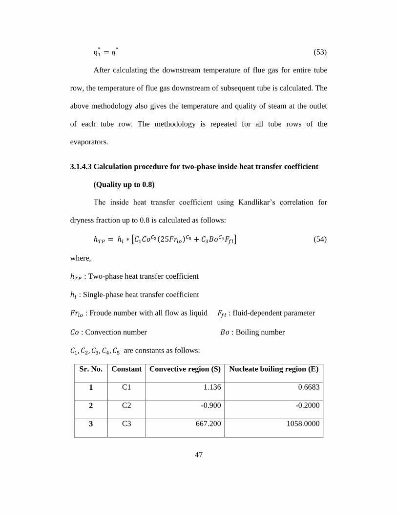
3.1.4.3 Calculation procedure for two-phase inside heat transfer coefficient
(Quality up to 0.8)
The inside heat transfer coefficient using Kandlikar‟s correlation for
dryness fraction up to 0.8 is calculated as follows:
(54)
where,
: Two-phase heat transfer coefficient
: Single-phase heat transfer coefficient
: Froude number with all flow as liquid : fluid-dependent parameter
: Convection number : Boiling number
are constants as follows:
Sr. No. Constant Convective region (S) Nucleate boiling region (E)
1 C1 1.136 0.6683
2 C2 -0.900 -0.2000
3 C3 667.200 1058.0000
48
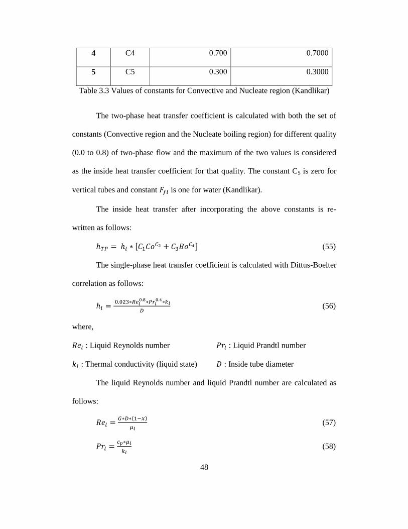
4 C4 0.700 0.7000
5 C5 0.300 0.3000
Table 3.3 Values of constants for Convective and Nucleate region (Kandlikar)
The two-phase heat transfer coefficient is calculated with both the set of
constants (Convective region and the Nucleate boiling region) for different quality
(0.0 to 0.8) of two-phase flow and the maximum of the two values is considered
as the inside heat transfer coefficient for that quality. The constant C5 is zero for
vertical tubes and constant is one for water (Kandlikar).
The inside heat transfer after incorporating the above constants is re-
written as follows:
(55)
The single-phase heat transfer coefficient is calculated with Dittus-Boelter
correlation as follows:
(56)
where,
: Liquid Reynolds number : Liquid Prandtl number
: Thermal conductivity (liquid state) : Inside tube diameter
The liquid Reynolds number and liquid Prandtl number are calculated as
follows:
(57)
(58)
49
where,
: Mass flux : Inside tube diameter
: Dryness fraction : dynamic viscosity (liquid)
: Specific heat
The convection number and boiling number are calculated as
follows:
(59)
(60)
where,
: Dryness fraction : Steam density (vapor)
: Water density (liquid) : Heat flux
: Latent heat of vaporization
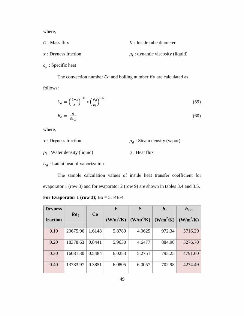
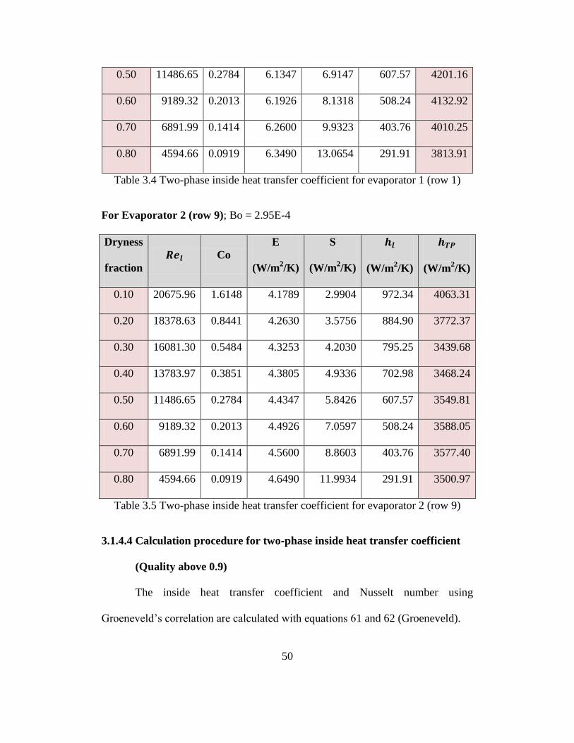
The sample calculation values of inside heat transfer coefficient for
evaporator 1 (row 3) and for evaporator 2 (row 9) are shown in tables 3.4 and 3.5.
For Evaporator 1 (row 3); Bo = 5.14E-4
Dryness
fraction
Co
E
(W/m2/K)
S
(W/m2/K)
(W/m2/K)
(W/m2/K)
0.10 20675.96 1.6148 5.8789 4.0625 972.34 5716.29
0.20 18378.63 0.8441 5.9630 4.6477 884.90 5276.70
0.30 16081.30 0.5484 6.0253 5.2751 795.25 4791.60
0.40 13783.97 0.3851 6.0805 6.0057 702.98 4274.49
50
0.50 11486.65 0.2784 6.1347 6.9147 607.57 4201.16
0.60 9189.32 0.2013 6.1926 8.1318 508.24 4132.92
0.70 6891.99 0.1414 6.2600 9.9323 403.76 4010.25
0.80 4594.66 0.0919 6.3490 13.0654 291.91 3813.91
Table 3.4 Two-phase inside heat transfer coefficient for evaporator 1 (row 1)
For Evaporator 2 (row 9); Bo = 2.95E-4
Dryness
fraction
Co
E
(W/m2/K)
S
(W/m2/K)
(W/m2/K)
(W/m2/K)
0.10 20675.96 1.6148 4.1789 2.9904 972.34 4063.31
0.20 18378.63 0.8441 4.2630 3.5756 884.90 3772.37
0.30 16081.30 0.5484 4.3253 4.2030 795.25 3439.68
0.40 13783.97 0.3851 4.3805 4.9336 702.98 3468.24
0.50 11486.65 0.2784 4.4347 5.8426 607.57 3549.81
0.60 9189.32 0.2013 4.4926 7.0597 508.24 3588.05
0.70 6891.99 0.1414 4.5600 8.8603 403.76 3577.40
0.80 4594.66 0.0919 4.6490 11.9934 291.91 3500.97
Table 3.5 Two-phase inside heat transfer coefficient for evaporator 2 (row 9)
3.1.4.4 Calculation procedure for two-phase inside heat transfer coefficient
(Quality above 0.9)
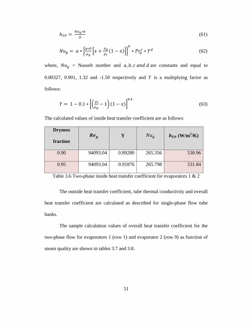
The inside heat transfer coefficient and Nusselt number using
Groeneveld‟s correlation are calculated with equations 61 and 62 (Groeneveld).
51
(61)
(62)
where, = Nusselt number and are constants and equal to
0.00327, 0.901, 1.32 and -1.50 respectively and is a multiplying factor as
follows:
(63)
The calculated values of inside heat transfer coefficient are as follows:
Dryness
fraction
Y (W/m2/K)
0.90 94093.04 0.89280 265.356 530.96
0.95 94093.04 0.91876 265.798 531.84
Table 3.6 Two-phase inside heat transfer coefficient for evaporators 1 & 2
The outside heat transfer coefficient, tube thermal conductivity and overall
heat transfer coefficient are calculated as described for single-phase flow tube
banks.
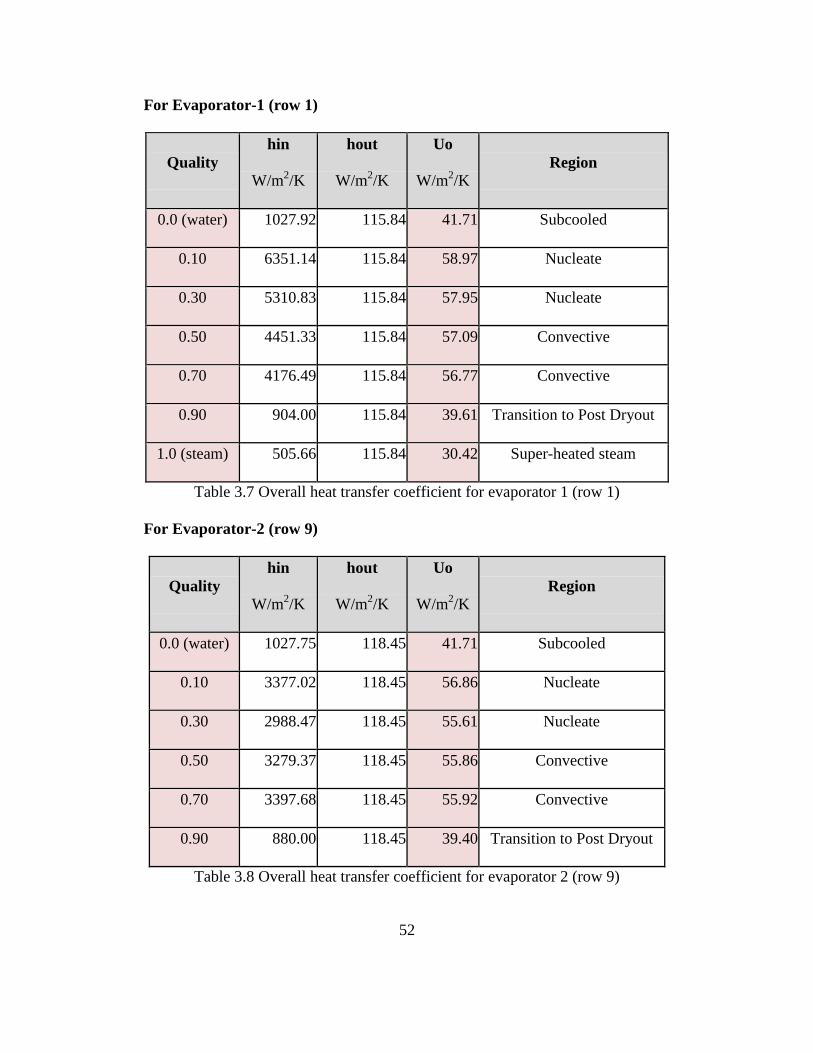
The sample calculation values of overall heat transfer coefficient for the
two-phase flow for evaporators 1 (row 1) and evaporator 2 (row 9) as function of
steam quality are shown in tables 3.7 and 3.8.
52
For Evaporator-1 (row 1)
Quality
hin
W/m2/K
hout
W/m2/K
Uo
W/m2/K
Region
0.0 (water) 1027.92 115.84 41.71 Subcooled
0.10 6351.14 115.84 58.97 Nucleate
0.30 5310.83 115.84 57.95 Nucleate
0.50 4451.33 115.84 57.09 Convective
0.70 4176.49 115.84 56.77 Convective
0.90 904.00 115.84 39.61 Transition to Post Dryout
1.0 (steam) 505.66 115.84 30.42 Super-heated steam
Table 3.7 Overall heat transfer coefficient for evaporator 1 (row 1)
For Evaporator-2 (row 9)
Quality
hin
W/m2/K
hout
W/m2/K
Uo
W/m2/K
Region
0.0 (water) 1027.75 118.45 41.71 Subcooled
0.10 3377.02 118.45 56.86 Nucleate
0.30 2988.47 118.45 55.61 Nucleate
0.50 3279.37 118.45 55.86 Convective
0.70 3397.68 118.45 55.92 Convective
0.90 880.00 118.45 39.40 Transition to Post Dryout
Table 3.8 Overall heat transfer coefficient for evaporator 2 (row 9)
53
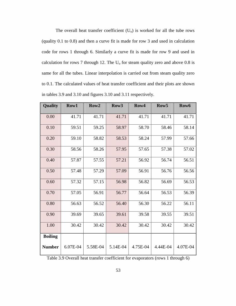
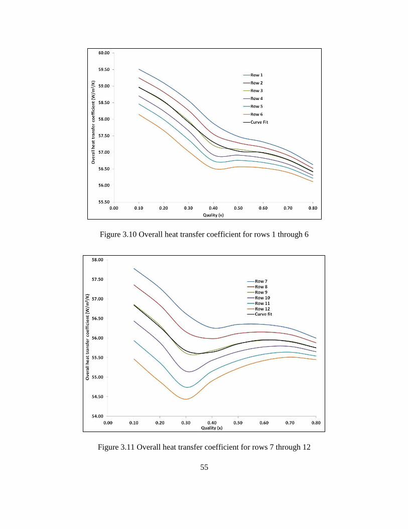
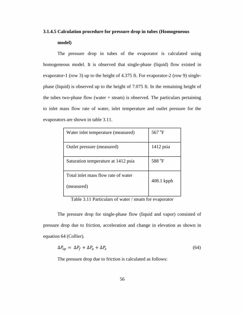
The overall heat transfer coefficient (Uo) is worked for all the tube rows
(quality 0.1 to 0.8) and then a curve fit is made for row 3 and used in calculation
code for rows 1 through 6. Similarly a curve fit is made for row 9 and used in
calculation for rows 7 through 12. The Uo for steam quality zero and above 0.8 is
same for all the tubes. Linear interpolation is carried out from steam quality zero
to 0.1. The calculated values of heat transfer coefficient and their plots are shown
in tables 3.9 and 3.10 and figures 3.10 and 3.11 respectively.
Quality Row1 Row2 Row3 Row4 Row5 Row6
0.00 41.71 41.71 41.71 41.71 41.71 41.71
0.10 59.51 59.25 58.97 58.70 58.46 58.14
0.20 59.10 58.82 58.53 58.24 57.99 57.66
0.30 58.56 58.26 57.95 57.65 57.38 57.02
0.40 57.87 57.55 57.21 56.92 56.74 56.51
0.50 57.48 57.29 57.09 56.91 56.76 56.56
0.60 57.32 57.15 56.98 56.82 56.69 56.53
0.70 57.05 56.91 56.77 56.64 56.53 56.39
0.80 56.63 56.52 56.40 56.30 56.22 56.11
0.90 39.69 39.65 39.61 39.58 39.55 39.51
1.00 30.42 30.42 30.42 30.42 30.42 30.42
Boiling
Number 6.07E-04 5.58E-04 5.14E-04 4.75E-04 4.44E-04 4.07E-04
Table 3.9 Overall heat transfer coefficient for evaporators (rows 1 through 6)
54
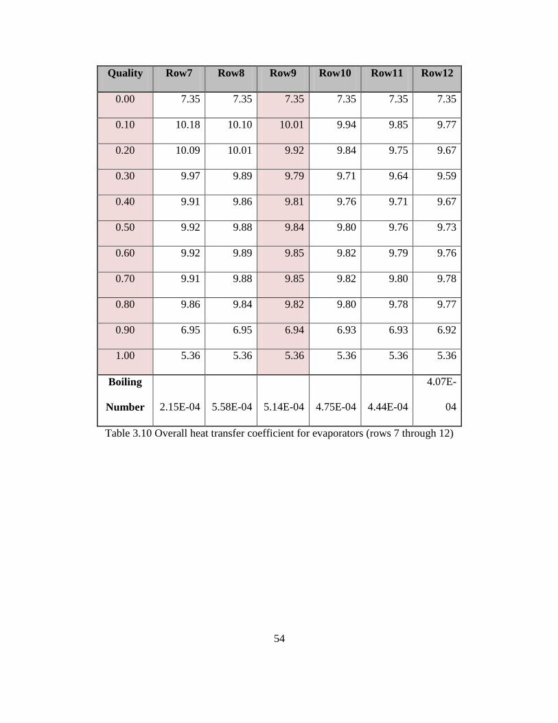
Quality Row7 Row8 Row9 Row10 Row11 Row12
0.00 7.35 7.35 7.35 7.35 7.35 7.35
0.10 10.18 10.10 10.01 9.94 9.85 9.77
0.20 10.09 10.01 9.92 9.84 9.75 9.67
0.30 9.97 9.89 9.79 9.71 9.64 9.59
0.40 9.91 9.86 9.81 9.76 9.71 9.67
0.50 9.92 9.88 9.84 9.80 9.76 9.73
0.60 9.92 9.89 9.85 9.82 9.79 9.76
0.70 9.91 9.88 9.85 9.82 9.80 9.78
0.80 9.86 9.84 9.82 9.80 9.78 9.77
0.90 6.95 6.95 6.94 6.93 6.93 6.92
1.00 5.36 5.36 5.36 5.36 5.36 5.36
Boiling
Number 2.15E-04 5.58E-04 5.14E-04 4.75E-04 4.44E-04
4.07E-
04
Table 3.10 Overall heat transfer coefficient for evaporators (rows 7 through 12)
55
Figure 3.10 Overall heat transfer coefficient for rows 1 through 6
Figure 3.11 Overall heat transfer coefficient for rows 7 through 12
56
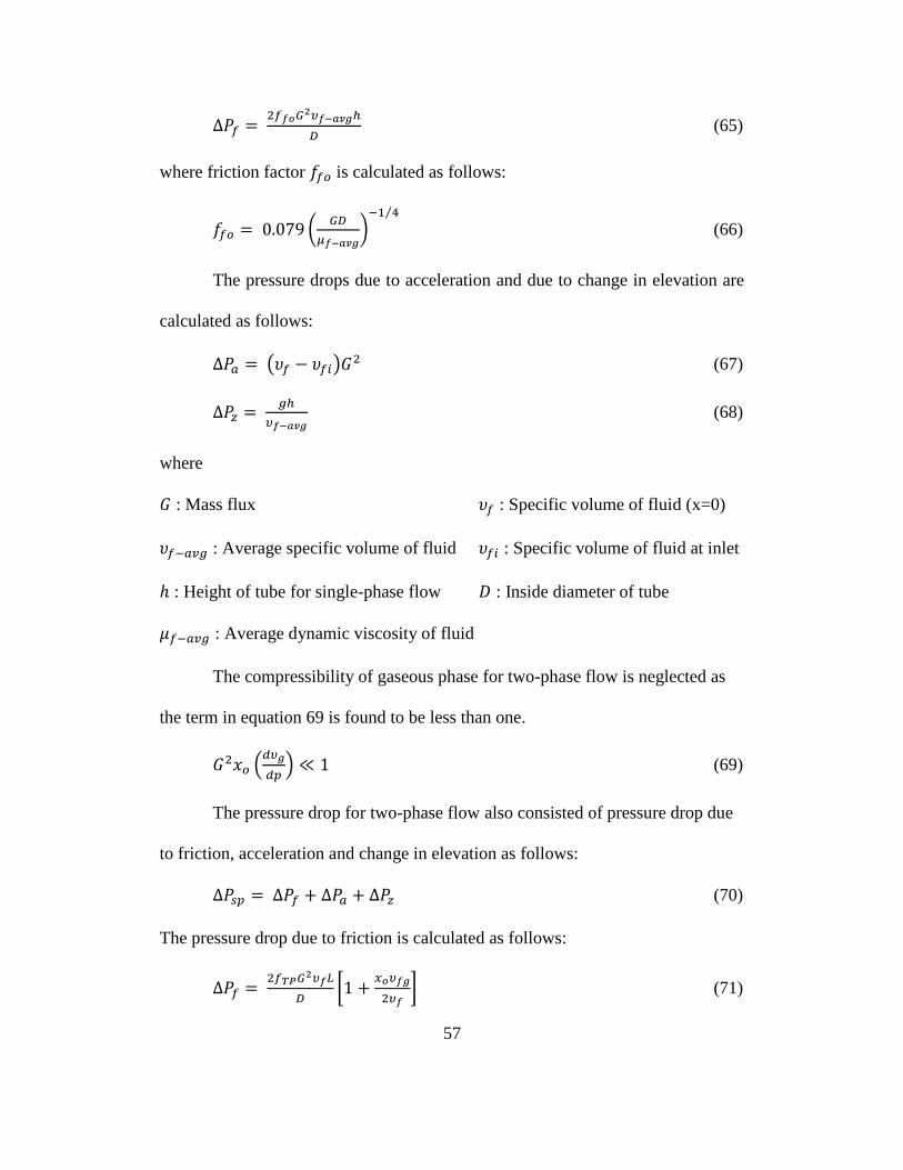
3.1.4.5 Calculation procedure for pressure drop in tubes (Homogeneous
model)
The pressure drop in tubes of the evaporator is calculated using
homogeneous model. It is observed that single-phase (liquid) flow existed in
evaporator-1 (row 3) up to the height of 4.375 ft. For evaporator-2 (row 9) single-
phase (liquid) is observed up to the height of 7.075 ft. In the remaining height of
the tubes two-phase flow (water + steam) is observed. The particulars pertaining
to inlet mass flow rate of water, inlet temperature and outlet pressure for the
evaporators are shown in table 3.11.
Water inlet temperature (measured) 567 oF
Outlet pressure (measured) 1412 psia
Saturation temperature at 1412 psia 588 oF
Total inlet mass flow rate of water
(measured)
408.1 kpph
Table 3.11 Particulars of water / steam for evaporator
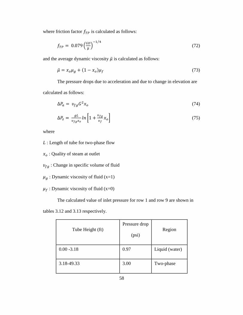
The pressure drop for single-phase flow (liquid and vapor) consisted of
pressure drop due to friction, acceleration and change in elevation as shown in
equation 64 (Collier).
(64)
The pressure drop due to friction is calculated as follows:
57
(65)
where friction factor is calculated as follows:
(66)
The pressure drops due to acceleration and due to change in elevation are
calculated as follows:
(67)
(68)
where
: Mass flux : Specific volume of fluid (x=0)
: Average specific volume of fluid : Specific volume of fluid at inlet
: Height of tube for single-phase flow : Inside diameter of tube
: Average dynamic viscosity of fluid
The compressibility of gaseous phase for two-phase flow is neglected as
the term in equation 69 is found to be less than one.
(69)
The pressure drop for two-phase flow also consisted of pressure drop due
to friction, acceleration and change in elevation as follows:
(70)
The pressure drop due to friction is calculated as follows:
(71)
58
where friction factor is calculated as follows:
(72)
and the average dynamic viscosity is calculated as follows:
(73)
The pressure drops due to acceleration and due to change in elevation are
calculated as follows:
(74)
(75)
where
: Length of tube for two-phase flow
: Quality of steam at outlet
: Change in specific volume of fluid
: Dynamic viscosity of fluid (x=1)
: Dynamic viscosity of fluid (x=0)
The calculated value of inlet pressure for row 1 and row 9 are shown in
tables 3.12 and 3.13 respectively.
Tube Height (ft)
Pressure drop
(psi)
Region
0.00 -3.18 0.97 Liquid (water)
3.18-49.33 3.00 Two-phase
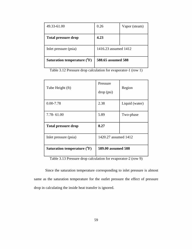
59
49.33-61.00 0.26 Vapor (steam)
Total pressure drop 4.23
Inlet pressure (psia) 1416.23 assumed 1412
Saturation temperature (oF) 588.65 assumed 588
Table 3.12 Pressure drop calculation for evaporator-1 (row 1)
Tube Height (ft)
Pressure
drop (psi)
Region
0.00-7.78 2.38 Liquid (water)
7.78- 61.00 5.89 Two-phase
Total pressure drop 8.27
Inlet pressure (psia) 1420.27 assumed 1412
Saturation temperature (oF) 589.00 assumed 588
Table 3.13 Pressure drop calculation for evaporator-2 (row 9)
Since the saturation temperature corresponding to inlet pressure is almost
same as the saturation temperature for the outlet pressure the effect of pressure
drop in calculating the inside heat transfer is ignored.
60
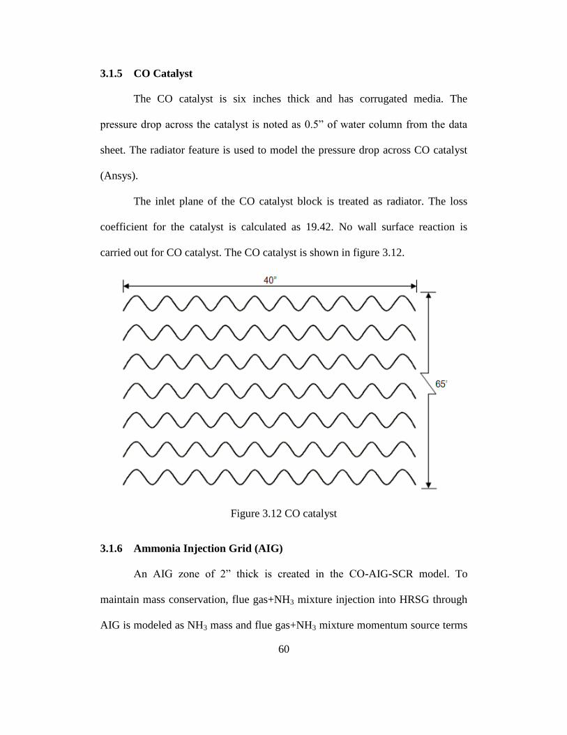
3.1.5 CO Catalyst
The CO catalyst is six inches thick and has corrugated media. The
pressure drop across the catalyst is noted as 0.5” of water column from the data
sheet. The radiator feature is used to model the pressure drop across CO catalyst
(Ansys).
The inlet plane of the CO catalyst block is treated as radiator. The loss
coefficient for the catalyst is calculated as 19.42. No wall surface reaction is
carried out for CO catalyst. The CO catalyst is shown in figure 3.12.
Figure 3.12 CO catalyst
3.1.6 Ammonia Injection Grid (AIG)
An AIG zone of 2” thick is created in the CO-AIG-SCR model. To
maintain mass conservation, flue gas+NH3 mixture injection into HRSG through
AIG is modeled as NH3 mass and flue gas+NH3 mixture momentum source terms
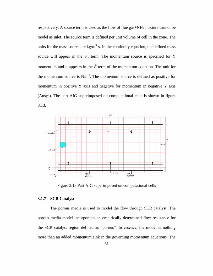
61
respectively. A source term is used as the flow of flue gas+NH3 mixture cannot be
model as inlet. The source term is defined per unit volume of cell in the zone. The
units for the mass source are kg/m3-s. In the continuity equation, the defined mass
source will appear in the Sm term. The momentum source is specified for Y
momentum and it appears in the term of the momentum equation. The unit for
the momentum source is N/m3. The momentum source is defined as positive for
momentum in positive Y axis and negative for momentum in negative Y axis
(Ansys). The part AIG superimposed on computational cells is shown in figure
3.13.
Figure 3.13 Part AIG superimposed on computational cells
3.1.7 SCR Catalyst
The porous media is used to model the flow through SCR catalyst. The
porous media model incorporates an empirically determined flow resistance for
the SCR catalyst region defined as “porous”. In essence, the model is nothing
more than an added momentum sink in the governing momentum equations. The
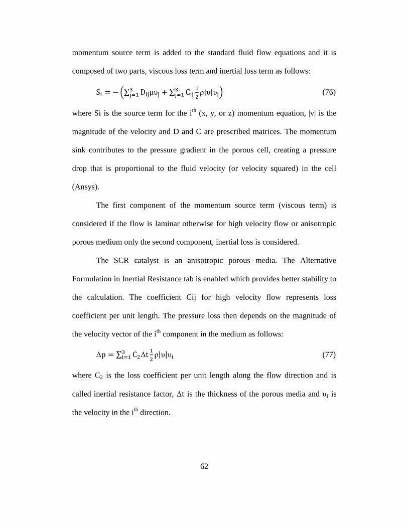
62
momentum source term is added to the standard fluid flow equations and it is
composed of two parts, viscous loss term and inertial loss term as follows:
(76)
where Si is the source term for the ith
(x, y, or z) momentum equation, |v| is the
magnitude of the velocity and D and C are prescribed matrices. The momentum
sink contributes to the pressure gradient in the porous cell, creating a pressure
drop that is proportional to the fluid velocity (or velocity squared) in the cell
(Ansys).
The first component of the momentum source term (viscous term) is
considered if the flow is laminar otherwise for high velocity flow or anisotropic
porous medium only the second component, inertial loss is considered.
The SCR catalyst is an anisotropic porous media. The Alternative
Formulation in Inertial Resistance tab is enabled which provides better stability to
the calculation. The coefficient Cij for high velocity flow represents loss
coefficient per unit length. The pressure loss then depends on the magnitude of
the velocity vector of the ith
component in the medium as follows:
(77)
where C2 is the loss coefficient per unit length along the flow direction and is
called inertial resistance factor, is the thickness of the porous media and is
the velocity in the ith
direction.
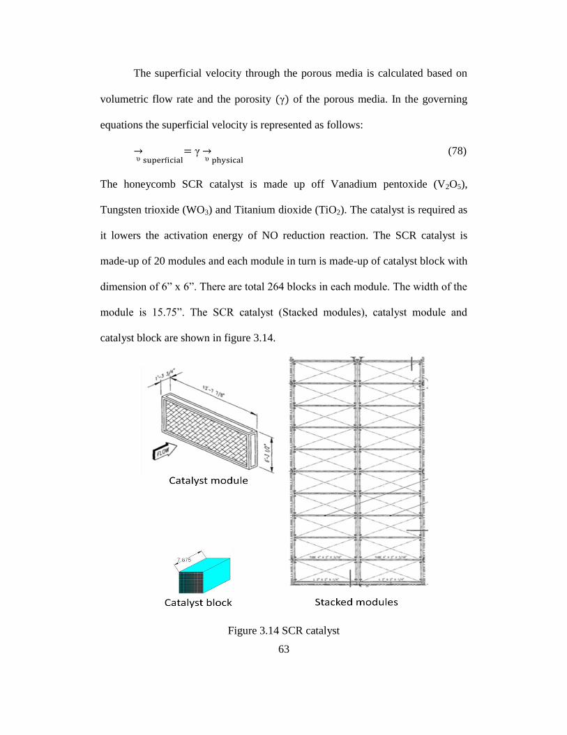
63
The superficial velocity through the porous media is calculated based on
volumetric flow rate and the porosity of the porous media. In the governing
equations the superficial velocity is represented as follows:
(78)
The honeycomb SCR catalyst is made up off Vanadium pentoxide (V2O5),
Tungsten trioxide (WO3) and Titanium dioxide (TiO2). The catalyst is required as
it lowers the activation energy of NO reduction reaction. The SCR catalyst is
made-up of 20 modules and each module in turn is made-up of catalyst block with
dimension of 6” x 6”. There are total 264 blocks in each module. The width of the
module is 15.75”. The SCR catalyst (Stacked modules), catalyst module and
catalyst block are shown in figure 3.14.
Figure 3.14 SCR catalyst
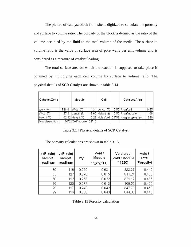
64
The picture of catalyst block from site is digitized to calculate the porosity
and surface to volume ratio. The porosity of the block is defined as the ratio of the
volume occupied by the fluid to the total volume of the media. The surface to
volume ratio is the value of surface area of pore walls per unit volume and is
considered as a measure of catalyst loading.
The total surface area on which the reaction is supposed to take place is
obtained by multiplying each cell volume by surface to volume ratio. The
physical details of SCR Catalyst are shown in table 3.14.
Table 3.14 Physical details of SCR Catalyst
The porosity calculations are shown in table 3.15.
Table 3.15 Porosity calculation
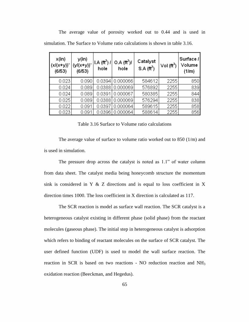
65
The average value of porosity worked out to 0.44 and is used in
simulation. The Surface to Volume ratio calculations is shown in table 3.16.
Table 3.16 Surface to Volume ratio calculations
The average value of surface to volume ratio worked out to 850 (1/m) and
is used in simulation.
The pressure drop across the catalyst is noted as 1.1” of water column
from data sheet. The catalyst media being honeycomb structure the momentum
sink is considered in Y & Z directions and is equal to loss coefficient in X
direction times 1000. The loss coefficient in X direction is calculated as 117.
The SCR reaction is model as surface wall reaction. The SCR catalyst is a
heterogeneous catalyst existing in different phase (solid phase) from the reactant
molecules (gaseous phase). The initial step in heterogeneous catalyst is adsorption
which refers to binding of reactant molecules on the surface of SCR catalyst. The
user defined function (UDF) is used to model the wall surface reaction. The
reaction in SCR is based on two reactions - NO reduction reaction and NH3
oxidation reaction (Beeckman, and Hegedus).
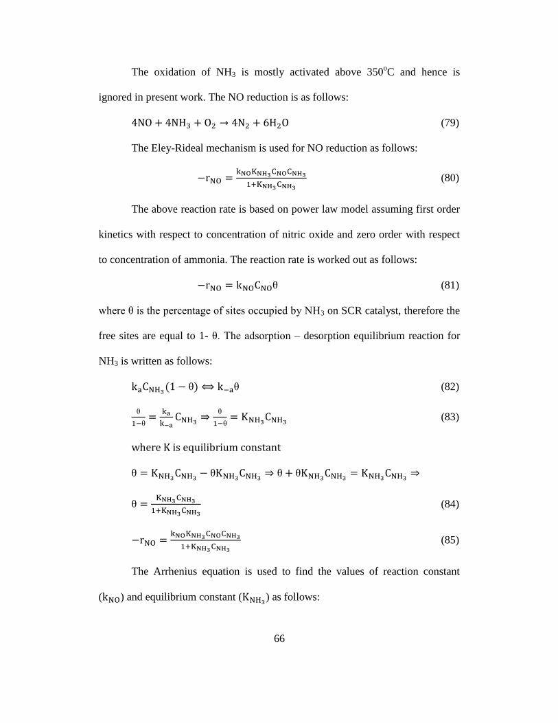
66
The oxidation of NH3 is mostly activated above 350oC and hence is
ignored in present work. The NO reduction is as follows:
(79)
The Eley-Rideal mechanism is used for NO reduction as follows:
(80)
The above reaction rate is based on power law model assuming first order
kinetics with respect to concentration of nitric oxide and zero order with respect
to concentration of ammonia. The reaction rate is worked out as follows:
(81)
where is the percentage of sites occupied by NH3 on SCR catalyst, therefore the
free sites are equal to 1- . The adsorption – desorption equilibrium reaction for
NH3 is written as follows:
(82)
(83)
(84)
(85)
The Arrhenius equation is used to find the values of reaction constant
( ) and equilibrium constant ( ) as follows:
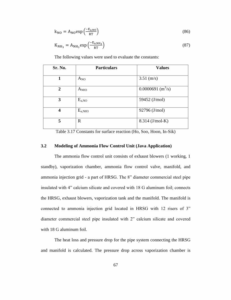
67
(86)
(87)
The following values were used to evaluate the constants:
Sr. No. Particulars Values
1 ANO 3.51 (m/s)
2 ANH3 0.0000691 (m3/s)
3 Ea,NO 59452 (J/mol)
4 Ea,NH3 92796 (J/mol)
5 R 8.314 (J/mol-K)
Table 3.17 Constants for surface reaction (Ho, Soo, Hoon, In-Sik)
3.2 Modeling of Ammonia Flow Control Unit (Java Application)
The ammonia flow control unit consists of exhaust blowers (1 working, 1
standby), vaporization chamber, ammonia flow control valve, manifold, and
ammonia injection grid - a part of HRSG. The 8” diameter commercial steel pipe
insulated with 4” calcium silicate and covered with 18 G aluminum foil; connects
the HRSG, exhaust blowers, vaporization tank and the manifold. The manifold is
connected to ammonia injection grid located in HRSG with 12 risers of 3”
diameter commercial steel pipe insulated with 2” calcium silicate and covered
with 18 G aluminum foil.
The heat loss and pressure drop for the pipe system connecting the HRSG
and manifold is calculated. The pressure drop across vaporization chamber is
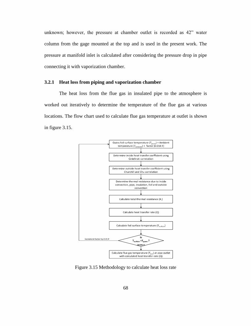
68
unknown; however, the pressure at chamber outlet is recorded as 42” water
column from the gage mounted at the top and is used in the present work. The
pressure at manifold inlet is calculated after considering the pressure drop in pipe
connecting it with vaporization chamber.
3.2.1 Heat loss from piping and vaporization chamber
The heat loss from the flue gas in insulated pipe to the atmosphere is
worked out iteratively to determine the temperature of the flue gas at various
locations. The flow chart used to calculate flue gas temperature at outlet is shown
in figure 3.15.
Figure 3.15 Methodology to calculate heat loss rate
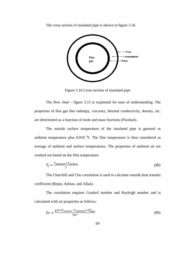
69
The cross section of insulated pipe is shown in figure 3.16.
Figure 3.16 Cross section of insulated pipe
The flow chart - figure 3.15 is explained for ease of understanding. The
properties of flue gas like enthalpy, viscosity, thermal conductivity, density, etc.
are determined as a function of mole and mass fractions (Flaxbart).
The outside surface temperature of the insulated pipe is guessed as
ambient temperature plus 0.018 oF. The film temperature is then considered as
average of ambient and surface temperatures. The properties of ambient air are
worked out based on the film temperature.
(88)
The Churchill and Chu correlation is used to calculate outside heat transfer
coefficient (Bejan, Adrian, and Allan).
The correlation requires Grashof number and Rayleigh number and is
calculated with air properties as follows:
(89)
70
(90)
For horizontal pipes
(91)
For vertical pipes
(92)
(93)
The Grashof number is analogous to the Reynolds number in forced
convection. The Gnielinski correlation is used to calculate inside heat transfer
coefficient. The correlation requires Prandtl number, Reynolds number and
friction factor and is calculated with flue gas properties as follows:
(94)
(95)
(96)
(97)
(98)
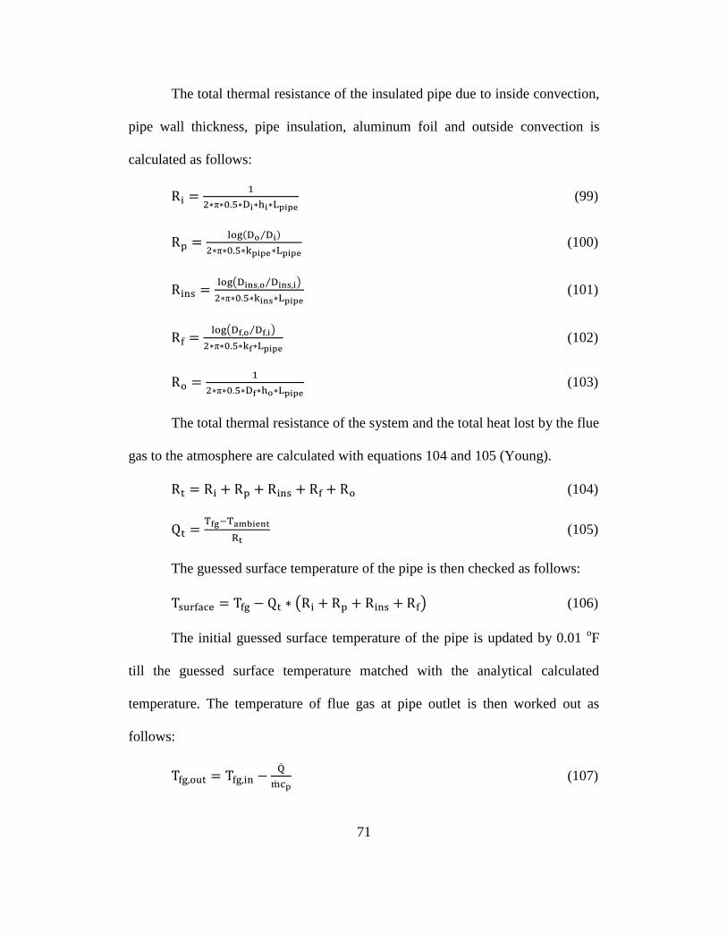
71
The total thermal resistance of the insulated pipe due to inside convection,
pipe wall thickness, pipe insulation, aluminum foil and outside convection is
calculated as follows:
(99)
(100)
(101)
(102)
(103)
The total thermal resistance of the system and the total heat lost by the flue
gas to the atmosphere are calculated with equations 104 and 105 (Young).
(104)
(105)
The guessed surface temperature of the pipe is then checked as follows:
(106)
The initial guessed surface temperature of the pipe is updated by 0.01 oF
till the guessed surface temperature matched with the analytical calculated
temperature. The temperature of flue gas at pipe outlet is then worked out as
follows:
(107)
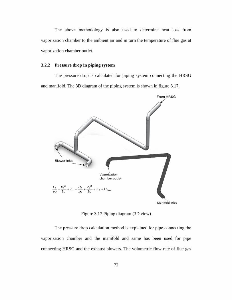
72
The above methodology is also used to determine heat loss from
vaporization chamber to the ambient air and in turn the temperature of flue gas at
vaporization chamber outlet.
3.2.2 Pressure drop in piping system
The pressure drop is calculated for piping system connecting the HRSG
and manifold. The 3D diagram of the piping system is shown in figure 3.17.
Figure 3.17 Piping diagram (3D view)
The pressure drop calculation method is explained for pipe connecting the
vaporization chamber and the manifold and same has been used for pipe
connecting HRSG and the exhaust blowers. The volumetric flow rate of flue gas
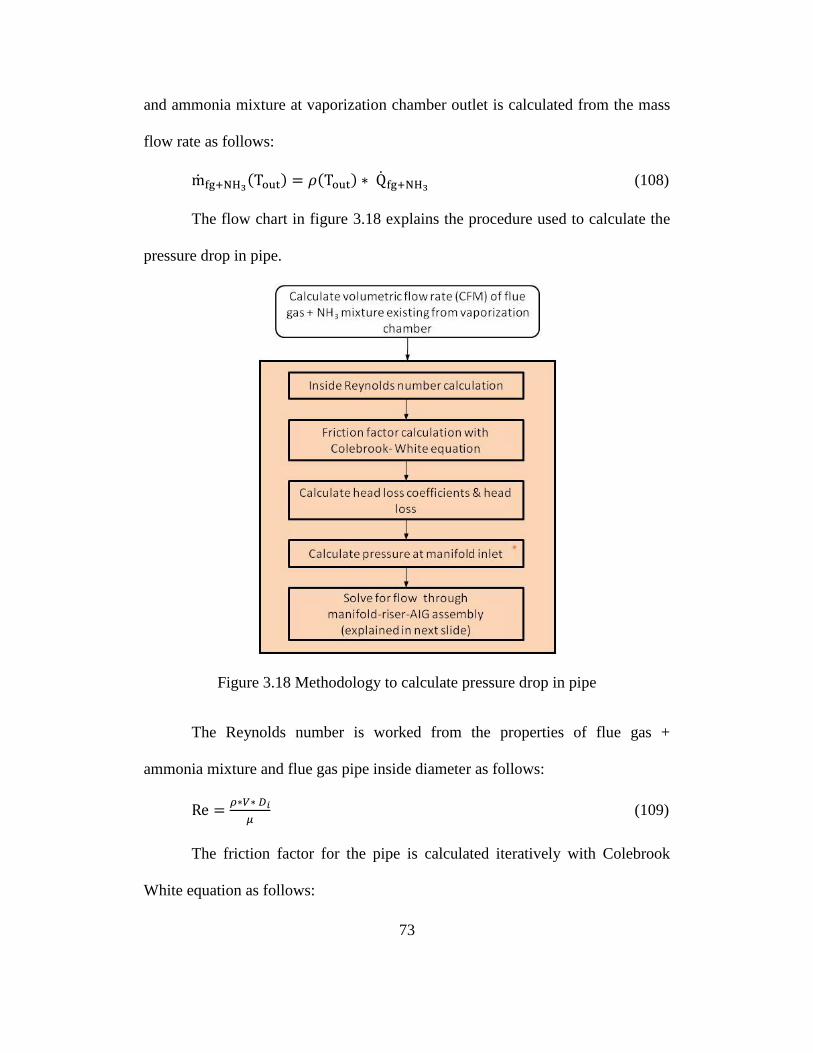
73
and ammonia mixture at vaporization chamber outlet is calculated from the mass
flow rate as follows:
(108)
The flow chart in figure 3.18 explains the procedure used to calculate the
pressure drop in pipe.
Figure 3.18 Methodology to calculate pressure drop in pipe
The Reynolds number is worked from the properties of flue gas +
ammonia mixture and flue gas pipe inside diameter as follows:
(109)
The friction factor for the pipe is calculated iteratively with Colebrook
White equation as follows:
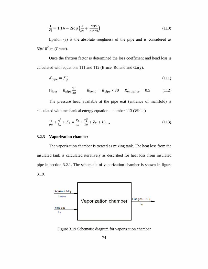
74
(110)
Epsilon (ε) is the absolute roughness of the pipe and is considered as
50x10-6
m (Crane).
Once the friction factor is determined the loss coefficient and head loss is
calculated with equations 111 and 112 (Bruce, Roland and Gary).
(111)
(112)
The pressure head available at the pipe exit (entrance of manifold) is
calculated with mechanical energy equation – number 113 (White).
(113)
3.2.3 Vaporization chamber
The vaporization chamber is treated as mixing tank. The heat loss from the
insulated tank is calculated iteratively as described for heat loss from insulated
pipe in section 3.2.1. The schematic of vaporization chamber is shown in figure
3.19.
Figure 3.19 Schematic diagram for vaporization chamber
75
The enthalpy of the flue gas consisting of nitrogen, oxygen, carbon
dioxide, water and argon is calculated as function of temperature. The enthalpy of
all the components are related to reference temperature as the enthalpy of
formation is based on reference temperature and pressure. The reference
temperature is 298 K and the reference pressure is 1 Atm. The enthalpy of flue
gas is calculated with equation 114 (Mench).
(114)
The quantity of aqueous ammonia (19% by weight) entering the
vaporization chamber is based on data sheet values as function of NOx
concentration at HRSG inlet. The enthalpy of aqueous ammonia as a function of
temperature i.e. ambient temperature is calculated as follows:
(115)
The temperature of flue gas and ammonia mixture at chamber outlet is
calculated iteratively as a function of net enthalpy. The net enthalpy of the flue
gas and ammonia mixture is calculated after considering the heat loss from the
vaporization chamber.
(116)
where,
(117)
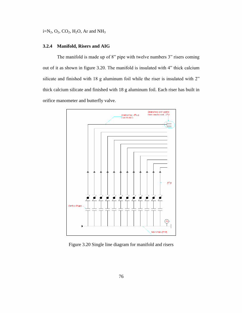
76
i=N2, O2, CO2, H2O, Ar and NH3
3.2.4 Manifold, Risers and AIG
The manifold is made up of 8” pipe with twelve numbers 3” risers coming
out of it as shown in figure 3.20. The manifold is insulated with 4” thick calcium
silicate and finished with 18 g aluminum foil while the riser is insulated with 2”
thick calcium silicate and finished with 18 g aluminum foil. Each riser has built in
orifice manometer and butterfly valve.
Figure 3.20 Single line diagram for manifold and risers
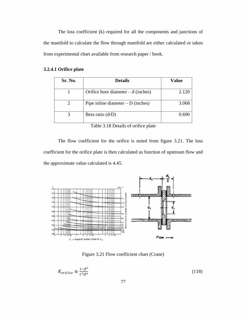
77
The loss coefficient (k) required for all the components and junctions of
the manifold to calculate the flow through manifold are either calculated or taken
from experimental chart available from research paper / book.
3.2.4.1 Orifice plate
Sr. No. Details Value
1 Orifice bore diameter – d (inches) 2.120
2 Pipe inline diameter – D (inches) 3.068
3 Beta ratio (d/D) 0.690
Table 3.18 Details of orifice plate
The flow coefficient for the orifice is noted from figure 3.21. The loss
coefficient for the orifice plate is then calculated as function of upstream flow and
the approximate value calculated is 4.45.
Figure 3.21 Flow coefficient chart (Crane)
(118)
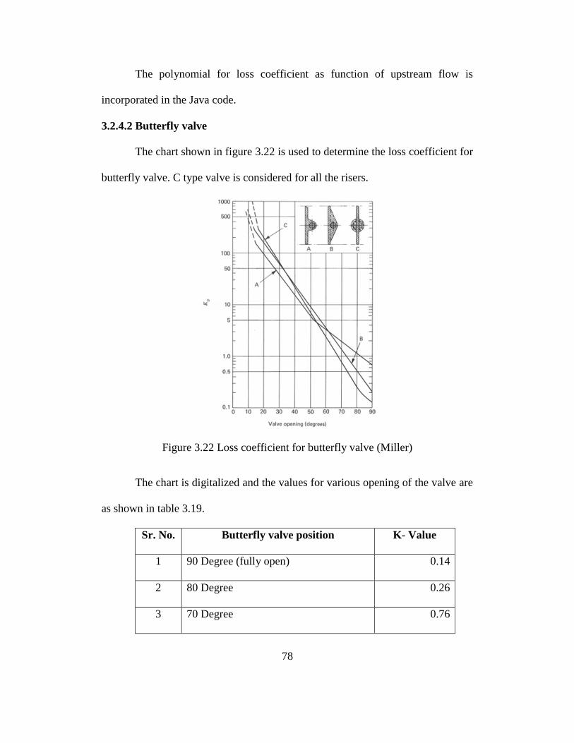
78
The polynomial for loss coefficient as function of upstream flow is
incorporated in the Java code.
3.2.4.2 Butterfly valve
The chart shown in figure 3.22 is used to determine the loss coefficient for
butterfly valve. C type valve is considered for all the risers.
Figure 3.22 Loss coefficient for butterfly valve (Miller)
The chart is digitalized and the values for various opening of the valve are
as shown in table 3.19.
Sr. No. Butterfly valve position K- Value
1 90 Degree (fully open) 0.14
2 80 Degree 0.26
3 70 Degree 0.76
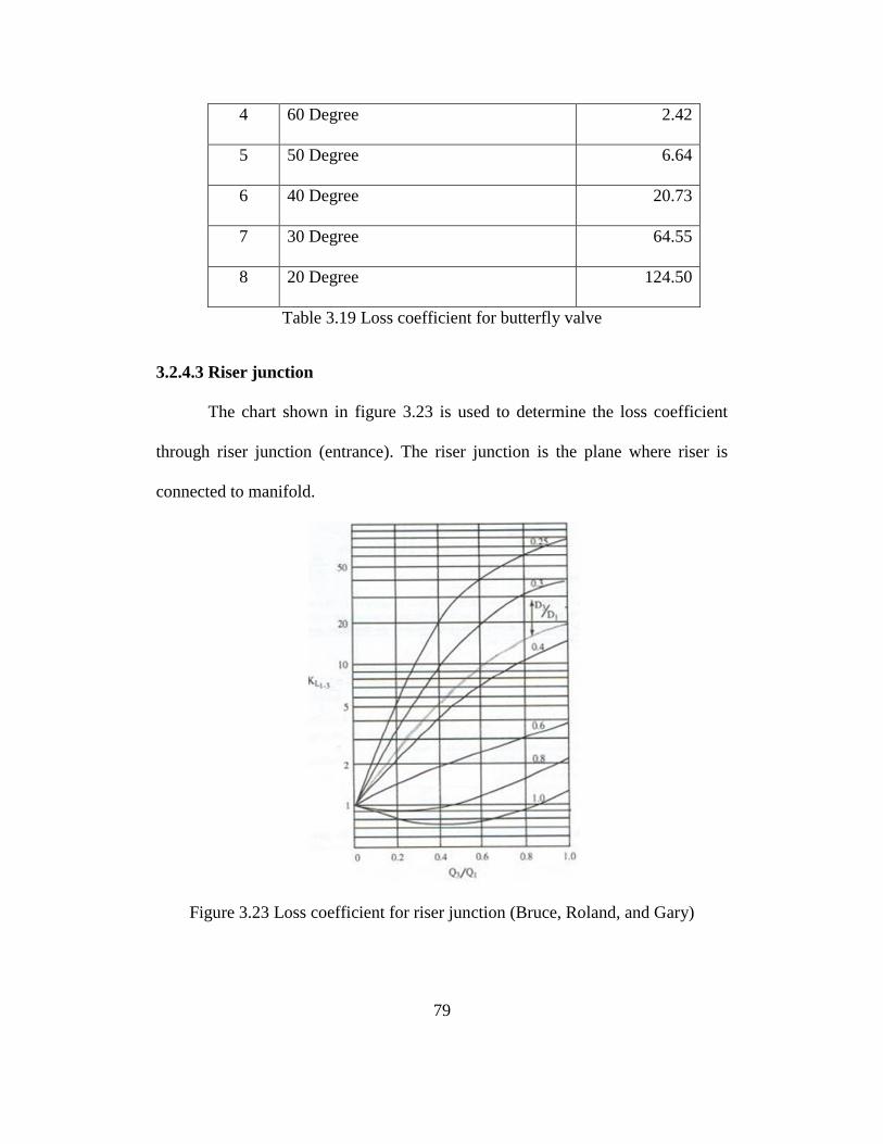
79
4 60 Degree 2.42
5 50 Degree 6.64
6 40 Degree 20.73
7 30 Degree 64.55
8 20 Degree 124.50
Table 3.19 Loss coefficient for butterfly valve
3.2.4.3 Riser junction
The chart shown in figure 3.23 is used to determine the loss coefficient
through riser junction (entrance). The riser junction is the plane where riser is
connected to manifold.
Figure 3.23 Loss coefficient for riser junction (Bruce, Roland, and Gary)
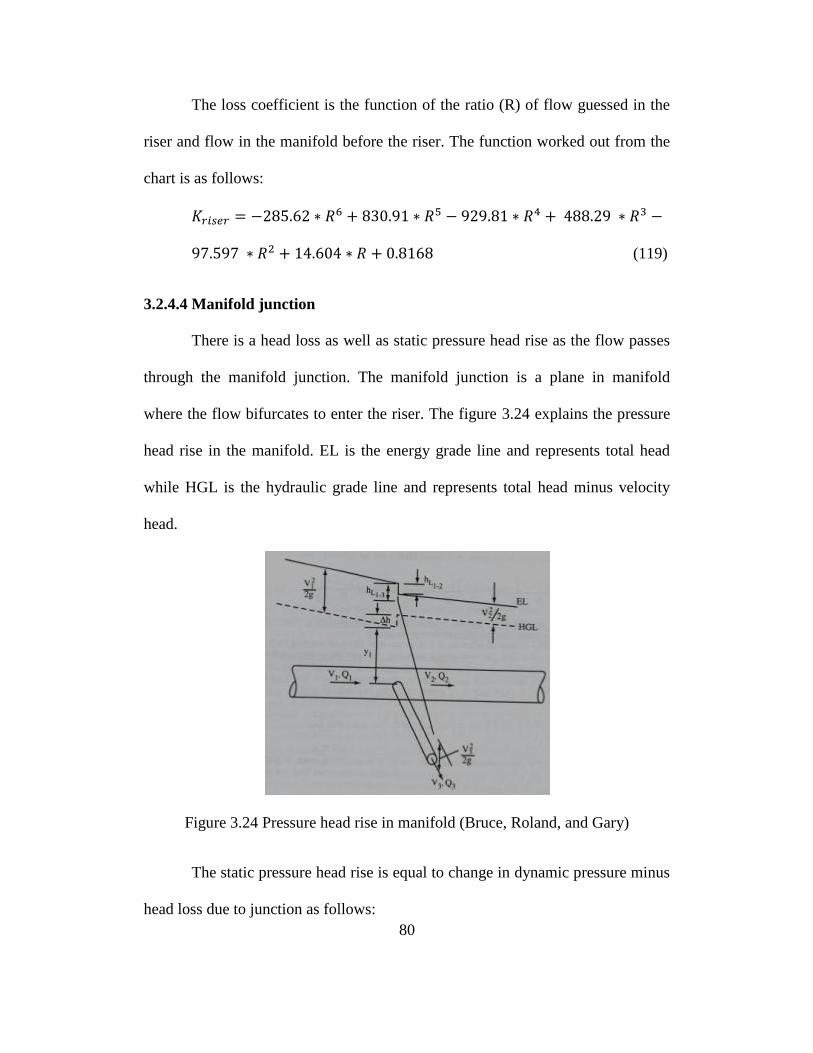
80
The loss coefficient is the function of the ratio (R) of flow guessed in the
riser and flow in the manifold before the riser. The function worked out from the
chart is as follows:
(119)
3.2.4.4 Manifold junction
There is a head loss as well as static pressure head rise as the flow passes
through the manifold junction. The manifold junction is a plane in manifold
where the flow bifurcates to enter the riser. The figure 3.24 explains the pressure
head rise in the manifold. EL is the energy grade line and represents total head
while HGL is the hydraulic grade line and represents total head minus velocity
head.
Figure 3.24 Pressure head rise in manifold (Bruce, Roland, and Gary)
The static pressure head rise is equal to change in dynamic pressure minus
head loss due to junction as follows:
81
(120)
The non dimensionalized pressure head rise chart as shown in figure 3.25
is digitized and the function of the ratio (R) of flow guessed in riser and flow in
the manifold before the riser for the given D3/D1 ratio (ration of riser and
manifold diameters) is calculated as follows:
(121)
Figure 3.25 Pressure head rise in manifold (Bruce, Roland, and Gary)
The non dimensionalized equation is written in terms of velocities and
flow rates as follows:
82
(122)
(123)
The non dimensionalized equation is re-arranged using continuity equation
as follows:
(124)
The chart shown in figure 3.26 is generated to determine the loss
coefficient through the manifold junction as function of flow ratio R. The function
worked out from the chart is as follows:
(125)
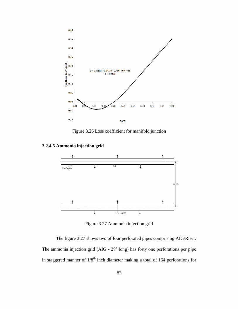
83
Figure 3.26 Loss coefficient for manifold junction
3.2.4.5 Ammonia injection grid
Figure 3.27 Ammonia injection grid
The figure 3.27 shows two of four perforated pipes comprising AIG/Riser.
The ammonia injection grid (AIG - 29‟ long) has forty one perforations per pipe
in staggered manner of 1/8th
inch diameter making a total of 164 perforations for
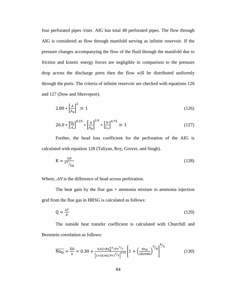
84
four perforated pipes /riser. AIG has total 48 perforated pipes. The flow through
AIG is considered as flow through manifold serving as infinite reservoir. If the
pressure changes accompanying the flow of the fluid through the manifold due to
friction and kinetic energy forces are negligible in comparison to the pressure
drop across the discharge ports then the flow will be distributed uniformly
through the ports. The criteria of infinite reservoir are checked with equations 126
and 127 (Dow and Shreveport).
(126)
(127)
Further, the head loss coefficient for the perforation of the AIG is
calculated with equation 128 (Taliyan, Roy, Grover, and Singh).
(128)
Where, ΔH is the difference of head across perforation.
The heat gain by the flue gas + ammonia mixture in ammonia injection
grid from the flue gas in HRSG is calculated as follows:
(129)
The outside heat transfer coefficient is calculated with Churchill and
Bernstein correlation as follows:
(130)
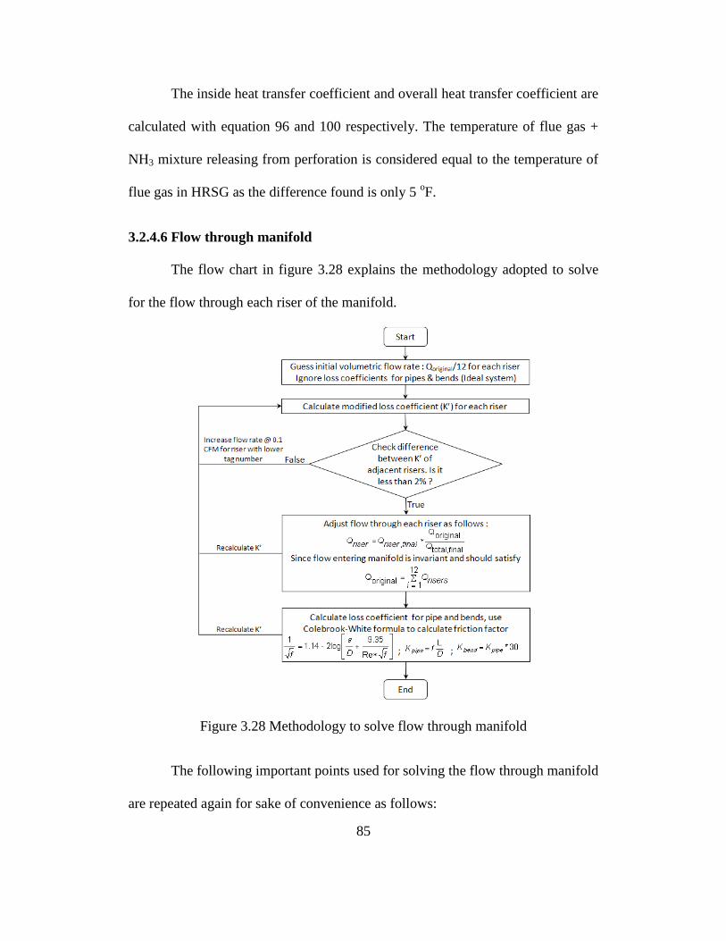
85
The inside heat transfer coefficient and overall heat transfer coefficient are
calculated with equation 96 and 100 respectively. The temperature of flue gas +
NH3 mixture releasing from perforation is considered equal to the temperature of
flue gas in HRSG as the difference found is only 5 oF.
3.2.4.6 Flow through manifold
The flow chart in figure 3.28 explains the methodology adopted to solve
for the flow through each riser of the manifold.
Figure 3.28 Methodology to solve flow through manifold
The following important points used for solving the flow through manifold
are repeated again for sake of convenience as follows:
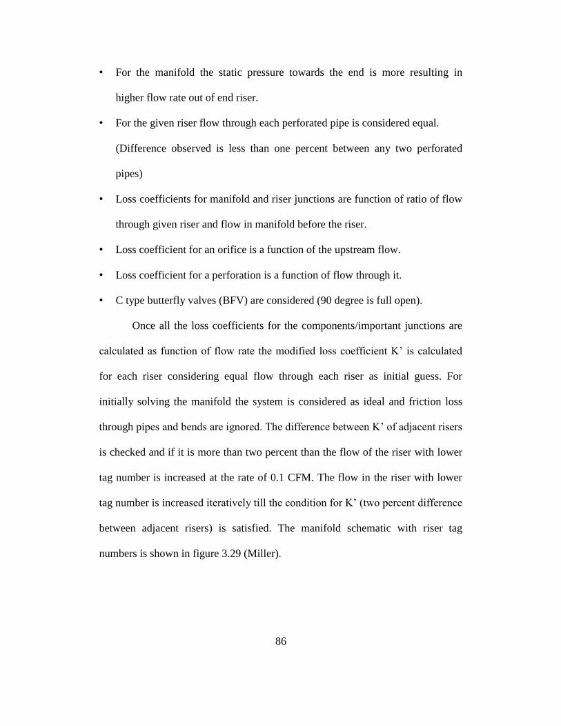
86
• For the manifold the static pressure towards the end is more resulting in
higher flow rate out of end riser.
• For the given riser flow through each perforated pipe is considered equal.
(Difference observed is less than one percent between any two perforated
pipes)
• Loss coefficients for manifold and riser junctions are function of ratio of flow
through given riser and flow in manifold before the riser.
• Loss coefficient for an orifice is a function of the upstream flow.
• Loss coefficient for a perforation is a function of flow through it.
• C type butterfly valves (BFV) are considered (90 degree is full open).
Once all the loss coefficients for the components/important junctions are
calculated as function of flow rate the modified loss coefficient K‟ is calculated
for each riser considering equal flow through each riser as initial guess. For
initially solving the manifold the system is considered as ideal and friction loss
through pipes and bends are ignored. The difference between K‟ of adjacent risers
is checked and if it is more than two percent than the flow of the riser with lower
tag number is increased at the rate of 0.1 CFM. The flow in the riser with lower
tag number is increased iteratively till the condition for K‟ (two percent difference
between adjacent risers) is satisfied. The manifold schematic with riser tag
numbers is shown in figure 3.29 (Miller).
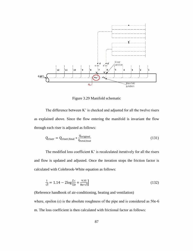
87
Figure 3.29 Manifold schematic
The difference between K‟ is checked and adjusted for all the twelve risers
as explained above. Since the flow entering the manifold is invariant the flow
through each riser is adjusted as follows:
(131)
The modified loss coefficient K‟ is recalculated iteratively for all the risers
and flow is updated and adjusted. Once the iteration stops the friction factor is
calculated with Colebrook-White equation as follows:
ε
(132)
(Reference handbook of air-conditioning, heating and ventilation)
where, epsilon (ε) is the absolute roughness of the pipe and is considered as 50e-6
m. The loss coefficient is then calculated with frictional factor as follows:
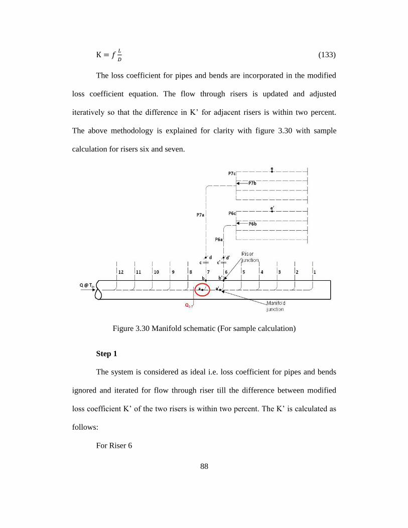
88
(133)
The loss coefficient for pipes and bends are incorporated in the modified
loss coefficient equation. The flow through risers is updated and adjusted
iteratively so that the difference in K‟ for adjacent risers is within two percent.
The above methodology is explained for clarity with figure 3.30 with sample
calculation for risers six and seven.
Figure 3.30 Manifold schematic (For sample calculation)
Step 1
The system is considered as ideal i.e. loss coefficient for pipes and bends
ignored and iterated for flow through riser till the difference between modified
loss coefficient K‟ of the two risers is within two percent. The K‟ is calculated as
follows:
For Riser 6
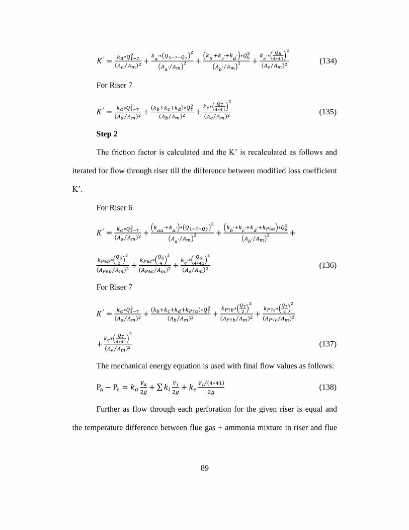
89
(134)
For Riser 7
(135)
Step 2
The friction factor is calculated and the K‟ is recalculated as follows and
iterated for flow through riser till the difference between modified loss coefficient
K‟.
For Riser 6
(136)
For Riser 7
(137)
The mechanical energy equation is used with final flow values as follows:
(138)
Further as flow through each perforation for the given riser is equal and
the temperature difference between flue gas + ammonia mixture in riser and flue

90
gas in HRSG is ignored, the flow through each perforation is calculated by taking
density ratios as follows:
(139)
91
CHAPTER 4
THE CFD TOOL
4.1 Fluent–Introduction
This chapter gives a general idea of the computational fluid dynamics tool,
Ansys–Fluent, used for simulation in this project. It describes the governing mass,
momentum and energy conservation equations, flow solver - pressure based
solver, K-ε turbulence model, standard wall function, cell zone and boundary
conditions.
Computational fluid dynamics (CFD) is the use of computer and
numerical methods to solve problems involving fluid flow. It is the analysis of
systems involving fluid flow, heat transfer and associated phenomena such as
chemical reactions by means of computer-based simulation.
This technique is very powerful and spans a wide range of industrial and
non-industrial application areas. The computational model is built in a meshing
tool, a preprocessor – ICEM and the boundary conditions are applied. The mesh is
then imported in Ansys Fluent for simulation.
Fluent is a CFD software package using C language to numerically solve
for fluid flow. It uses finite volume method to solve the governing equations of
fluid flow. The software has the capability to solve for flow in 2D and 3D
geometry.
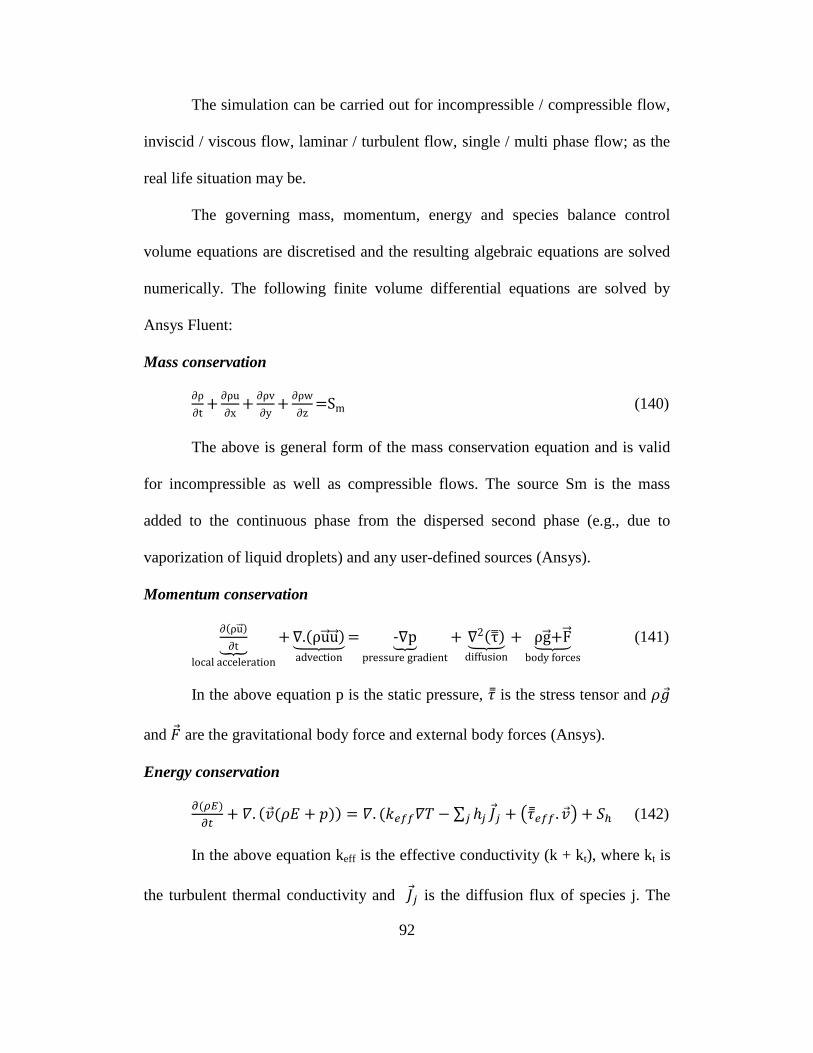
92
The simulation can be carried out for incompressible / compressible flow,
inviscid / viscous flow, laminar / turbulent flow, single / multi phase flow; as the
real life situation may be.
The governing mass, momentum, energy and species balance control
volume equations are discretised and the resulting algebraic equations are solved
numerically. The following finite volume differential equations are solved by
Ansys Fluent:
Mass conservation
(140)
The above is general form of the mass conservation equation and is valid
for incompressible as well as compressible flows. The source Sm is the mass
added to the continuous phase from the dispersed second phase (e.g., due to
vaporization of liquid droplets) and any user-defined sources (Ansys).
Momentum conservation
-
(141)
In the above equation p is the static pressure, is the stress tensor and
and are the gravitational body force and external body forces (Ansys).
Energy conservation
(142)
In the above equation keff is the effective conductivity (k + kt), where kt is
the turbulent thermal conductivity and is the diffusion flux of species j. The
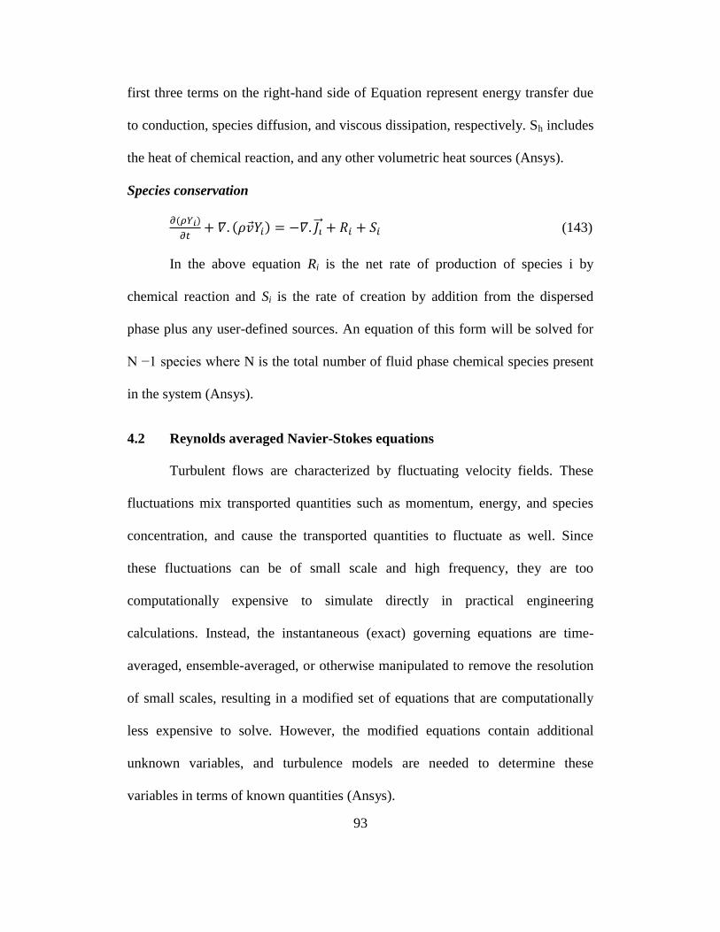
93
first three terms on the right-hand side of Equation represent energy transfer due
to conduction, species diffusion, and viscous dissipation, respectively. Sh includes
the heat of chemical reaction, and any other volumetric heat sources (Ansys).
Species conservation
(143)
In the above equation Ri is the net rate of production of species i by
chemical reaction and Si is the rate of creation by addition from the dispersed
phase plus any user-defined sources. An equation of this form will be solved for
N −1 species where N is the total number of fluid phase chemical species present
in the system (Ansys).
4.2 Reynolds averaged Navier-Stokes equations
Turbulent flows are characterized by fluctuating velocity fields. These
fluctuations mix transported quantities such as momentum, energy, and species
concentration, and cause the transported quantities to fluctuate as well. Since
these fluctuations can be of small scale and high frequency, they are too
computationally expensive to simulate directly in practical engineering
calculations. Instead, the instantaneous (exact) governing equations are time-
averaged, ensemble-averaged, or otherwise manipulated to remove the resolution
of small scales, resulting in a modified set of equations that are computationally
less expensive to solve. However, the modified equations contain additional
unknown variables, and turbulence models are needed to determine these
variables in terms of known quantities (Ansys).
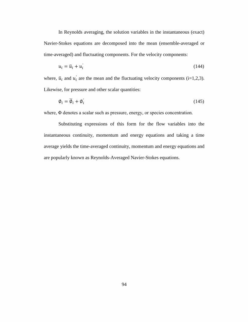
94
In Reynolds averaging, the solution variables in the instantaneous (exact)
Navier-Stokes equations are decomposed into the mean (ensemble-averaged or
time-averaged) and fluctuating components. For the velocity components:
(144)
where, and are the mean and the fluctuating velocity components (i=1,2,3).
Likewise, for pressure and other scalar quantities:
(145)
where, Φ denotes a scalar such as pressure, energy, or species concentration.
Substituting expressions of this form for the flow variables into the
instantaneous continuity, momentum and energy equations and taking a time
average yields the time-averaged continuity, momentum and energy equations and
are popularly known as Reynolds-Averaged Navier-Stokes equations.
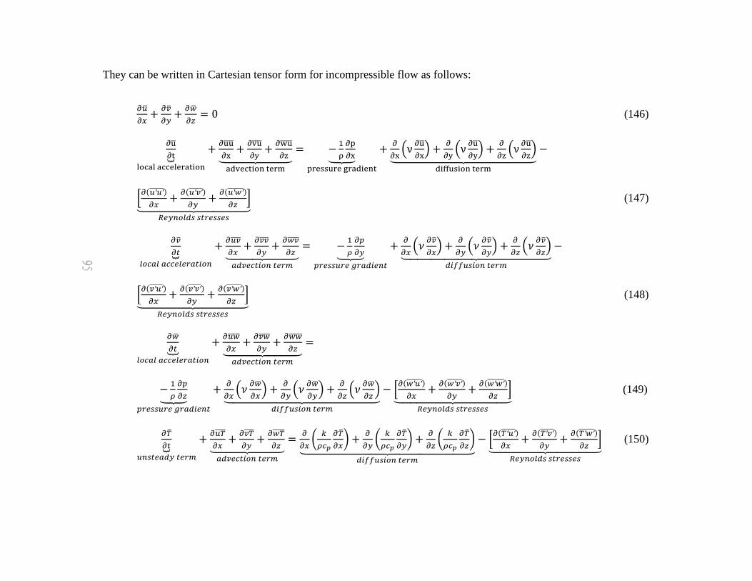
95
They can be written in Cartesian tensor form for incompressible flow as follows:
(146)
(147)
(148)
(149)
(150)
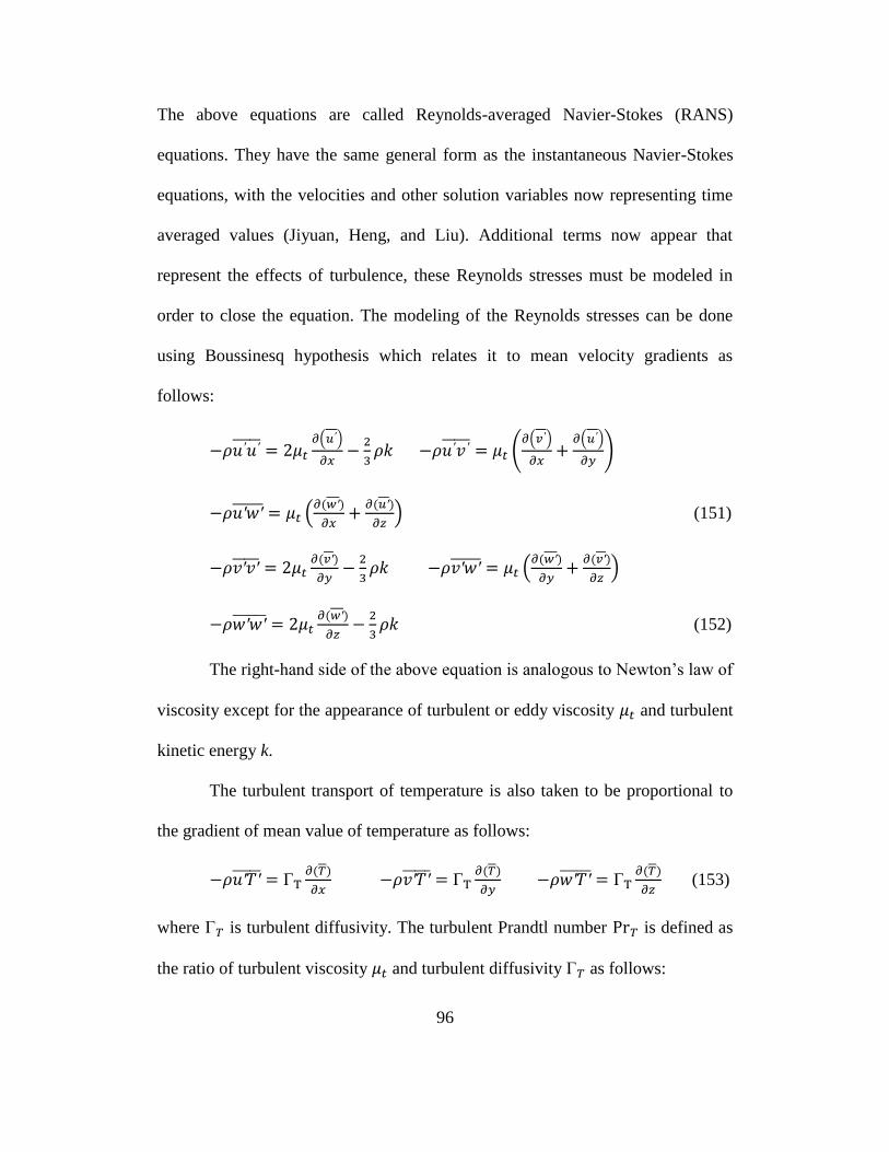
96
The above equations are called Reynolds-averaged Navier-Stokes (RANS)
equations. They have the same general form as the instantaneous Navier-Stokes
equations, with the velocities and other solution variables now representing time
averaged values (Jiyuan, Heng, and Liu). Additional terms now appear that
represent the effects of turbulence, these Reynolds stresses must be modeled in
order to close the equation. The modeling of the Reynolds stresses can be done
using Boussinesq hypothesis which relates it to mean velocity gradients as
follows:
(151)
(152)
The right-hand side of the above equation is analogous to Newton‟s law of
viscosity except for the appearance of turbulent or eddy viscosity and turbulent
kinetic energy k.
The turbulent transport of temperature is also taken to be proportional to
the gradient of mean value of temperature as follows:
(153)
where is turbulent diffusivity. The turbulent Prandtl number is defined as
the ratio of turbulent viscosity and turbulent diffusivity as follows:
97
(154)
The value of turbulent diffusivity is taken to be close to the value of
turbulent viscosity since the turbulent transport of momentum and heat is due
to same mechanism – eddy mixing and hence the value of turbulent Prandtl
number is taken close to unity. The standard k-ε model was used to calculate
turbulent viscosity in this work.
4.3 Turbulence model
4.3.1 The standard k-ε model
There is no single turbulence model universally accepted for all kinds of
problems. The selection of turbulence model depends on the physics encompassed
in the flow, level of accuracy required, available computational resources and the
amount of time available for simulation. The turbulence model is required to
solve for turbulent viscosity, µt. The standard k-ε model is used to calculate
turbulent viscosity as a function of turbulent kinetic energy k and turbulent
dissipation rate ε (Jiyuan, Heng, and Liu).
The standard k-ε model is a semi-empirical model based on model
transport equations for the turbulence kinetic energy (k) and its dissipation rate
(ε). The model transport equation for k is derived from the exact equation, while
the model transport equation for ε was obtained using physical reasoning and
bears little resemblance to its mathematically exact counterpart. The standard k-ε
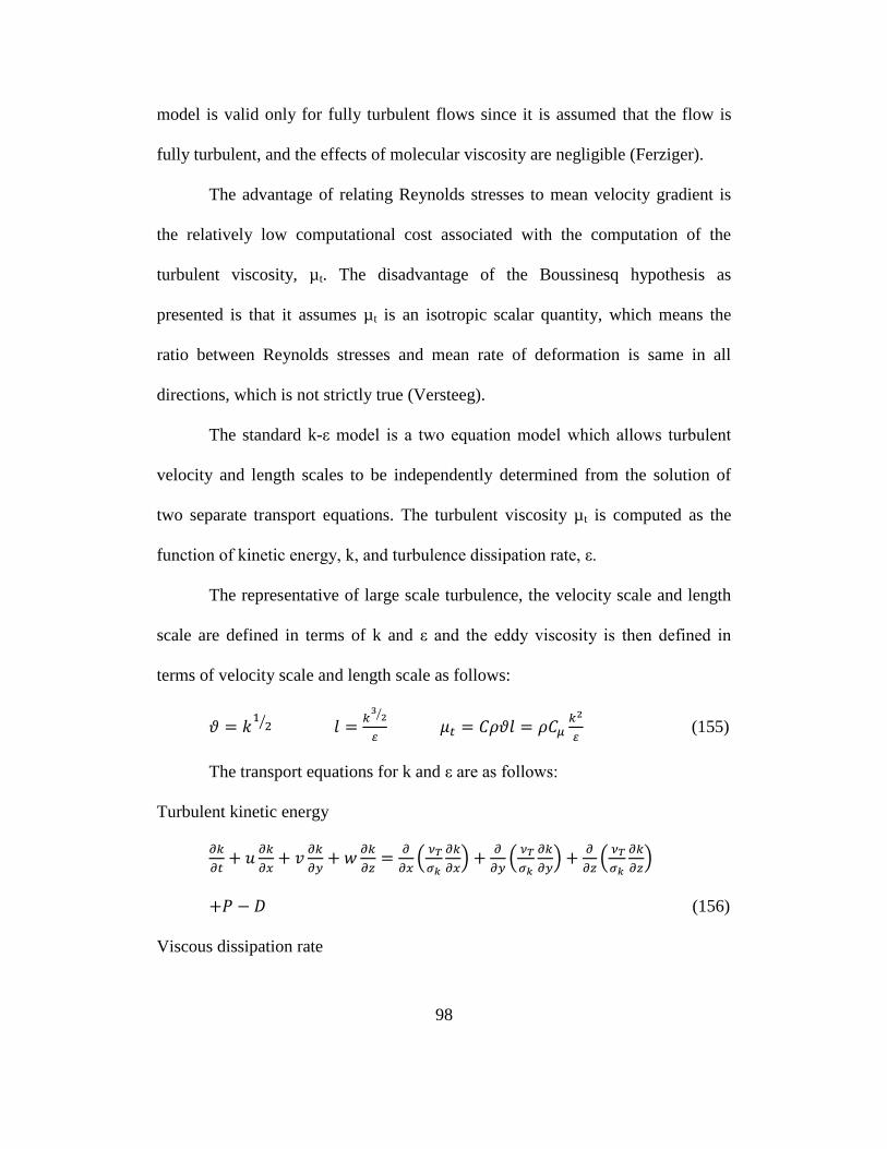
98
model is valid only for fully turbulent flows since it is assumed that the flow is
fully turbulent, and the effects of molecular viscosity are negligible (Ferziger).
The advantage of relating Reynolds stresses to mean velocity gradient is
the relatively low computational cost associated with the computation of the
turbulent viscosity, µt. The disadvantage of the Boussinesq hypothesis as
presented is that it assumes µt is an isotropic scalar quantity, which means the
ratio between Reynolds stresses and mean rate of deformation is same in all
directions, which is not strictly true (Versteeg).
The standard k-ε model is a two equation model which allows turbulent
velocity and length scales to be independently determined from the solution of
two separate transport equations. The turbulent viscosity µt is computed as the
function of kinetic energy, k, and turbulence dissipation rate, ε.
The representative of large scale turbulence, the velocity scale and length
scale are defined in terms of k and ε and the eddy viscosity is then defined in
terms of velocity scale and length scale as follows:
(155)
The transport equations for k and ε are as follows:
Turbulent kinetic energy
(156)
Viscous dissipation rate
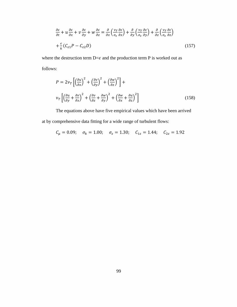
99
(157)
where the destruction term D= and the production term P is worked out as
follows:
(158)
The equations above have five empirical values which have been arrived
at by comprehensive data fitting for a wide range of turbulent flows:
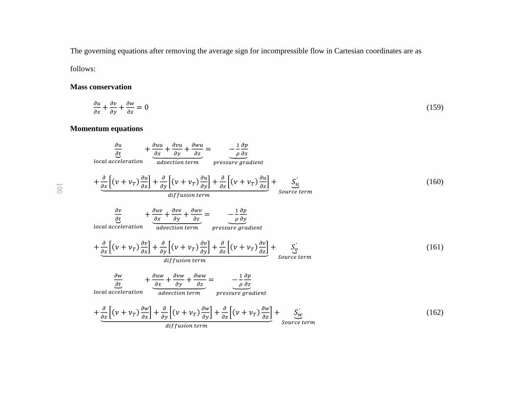
100
The governing equations after removing the average sign for incompressible flow in Cartesian coordinates are as
follows:
Mass conservation
(159)
Momentum equations
(160)
(161)
(162)
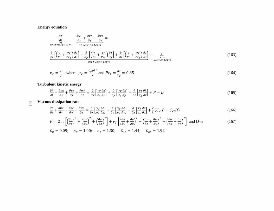
101
Energy equation
(163)
where
and
(164)
Turbulent kinetic energy
(165)
Viscous dissipation rate
(166)
and D= (167)
102
4.3.2 Near-wall model
The accurate representation of the turbulent flow in the near wall region
determines successful simulation of wall bounded turbulent flow.
Very close to the wall, viscous damping reduces the tangential velocity
fluctuations and kinematic blocking reduces the normal fluctuations.
Turbulence is rapidly increased by the production of turbulence kinetic
energy due to the large gradients in mean velocity toward the outer part of the
near-wall region.
In Ansys fluent there are two approaches for near wall region modeling. In
one approach, the viscosity-affected inner region (viscous sub-layer and buffer
layer) is not resolved and semi-empirical formulas called “wall functions” are
used to bridge the viscosity-affected region between the wall and the fully-
turbulent region.
The use of wall functions obviates the need to modify the turbulence
models to account for the presence of the wall (Ansys).
In another approach, the turbulence models are modified to enable the
viscosity-affected region to be resolved with a mesh all the way to the wall,
including the viscous sub-layer. This is termed as “near-wall modeling” approach.
The standard wall function has been used in this project work as it saves
computational resources as the viscosity affected region in which the solution
variables change most rapidly is not required to be resolved.
The standard wall function
103
Momentum
The momentum balance for the near-wall cell requires the wall shear
stress . Since the near-wall region isn‟t resolved, this requires some assumption
about what goes on between near-wall node and the surface. The law of the wall
for mean velocity yields
(168)
Where, U* the non-dimensionalized velocity and y* the non-dimensionalized
distance from the wall and are given as under:
(169)
(170)
where is von Karman constant (0.42), E is function of wall roughness and equal
to 9.73 for smooth walls, Up is mean velocity of fluid at node P (first near wall
node), is turbulence kinetic energy at node P, yp is distance of point P from
wall and µ is dynamic viscosity if the fluid.
Energy
The law of the wall is applied to determine wall temperature (Tw).
(171)
where is turbulent kinetic energy at node P(first near wall node), is fluid
density, cp is fluid specific heat, is wall heat flux, Tp is temperature at node P,
Tw is wall temperature.
104
Species
The wall function for species transport assumes that species transport
behaves analogously to heat transfer and is expressed for constant property flow
with no viscous dissipation as follows:
(172)
where Yi is the local species mass fraction and Ji,w is the diffusion flux of species
i at the wall.
4.4 Flow solver:
Ansys Fluent has two flow solvers to choose from:
1) Pressure-based solver
2) Density-based solver
Both the solvers have been updated and can be used for wide range of
flow conditions. The pressure based solver was meant for low speed
incompressible flow while the density based was meant for high speed
compressible flow.
In both the approach the velocity is obtained from momentum equations.
For the density based solver the density field is obtained from continuity equation
and the pressure field from equation of state. However in pressure based approach
the pressure correction equation is solved for pressure field. The pressure
correction equation is obtained from continuity and momentum equations.
105
Using either method, ANSYS FLUENT will solve the governing integral
equations for the conservation of mass and momentum, and (when appropriate)
for energy and other scalars such as turbulence and chemical species. In both
cases a control-volume-based technique is used that consists of:
• Division of the domain into discrete control volumes using a
computational grid.
• Integration of the governing equations on the individual control volumes
to construct algebraic equations for the discrete dependent variables
(“unknowns”) such as velocities, pressure, temperature, and conserved
scalars.
• Linearization of the discretized equations and solution of the resultant
linear equation system to yield updated values of the dependent variables.
The two numerical methods employ a similar discretization process
(finite-volume), but the approach used to linearize and solve the discretized
equations is different [Fluent].
Due to incompressible assumption the solution to governing equations
becomes complicated due to absence of independent equation for pressure. The
flow is driven by pressure gradient in each momentum equations. With continuity
equation we have four equations and four unknowns and no independent equation
for pressure. The implication here is that the continuity and momentum equations
are all required to solve for the velocity and pressure fields in an incompressible
flow. In the present work pressure based solver is used.
106
4.4.1 Pressure-Based Solver
The pressure-based solver employs an algorithm which belongs to a
general class of methods called the projection method. In the projection method,
wherein the constraint of mass conservation (continuity) of the velocity field is
achieved by solving a pressure (or pressure correction) equation. The pressure
equation is derived from the continuity and the momentum equations in such a
way that the velocity field, corrected by the pressure, satisfies the continuity.
Since the governing equations are nonlinear and coupled to one another, the
solution process involves iterations wherein the entire set of governing equations
is solved repeatedly until the solution converges. ANSYS FLUENT uses a co-
located scheme, whereby pressure and velocity are both stored at cell centers
(Ansys).
Ansys Fluent has two pressure based solvers namely segregated and
coupled. In the present work pressure based segregated solver is used in which the
governing equations are solved sequentially. Because the governing equations are
non-linear and coupled, the solution loop is carried out iteratively in order to
obtain a converged numerical solution.
In the segregated algorithm, the individual governing equations for the
solution variables (e.g., u, v, w, p, T, k, ε, etc.) are solved one after another. Each
governing equation, while being solved, is “decoupled” or “segregated” from
other equations. The segregated algorithm is memory-efficient, since the
107
discretized equations need to be stored in the memory only once at a time
[Fluent].
Ansys Fluent has five pressure velocity coupling algorithms: SIMPLE,
SIMPLEC, PISO, Coupled, and Fractional Step (FSM). In the present work
SIMPLE algorithm (Semi-Implicit Method for Pressure-Linkage Equations) was
used for velocity pressure coupling. The steps of SIMPLE algorithm are explained
as follows:
1) In this method the momentum equations are solved using guessed pressure
field p*and velocity components u*, v* and w*. The solution of
discretized momentum equations yield updated velocity components u*,
v* and w*.
2) The correction is defined as the difference between the correct value and
the guessed value for pressure and velocity as follows:
p p p u u u v v v w w w (173)
3) Calculate coefficients and source terms for pressure correction equation.
4) Solve for pressure correction p‟ using the pressure correction equation,
which is a discretized continuity equation.
5) Then solve for correct pressure and velocity components using pressure
correction p‟.
6) The discretized transport equations are solved using the correct pressure
and velocity components and checked for convergence.
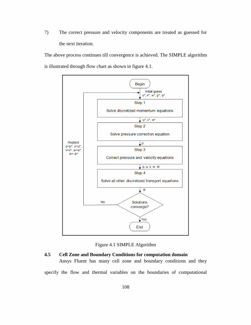
108
7) The correct pressure and velocity components are treated as guessed for
the next iteration.
The above process continues till convergence is achieved. The SIMPLE algorithm
is illustrated through flow chart as shown in figure 4.1.
Figure 4.1 SIMPLE Algorithm
4.5 Cell Zone and Boundary Conditions for computation domain
Ansys Fluent has many cell zone and boundary conditions and they
specify the flow and thermal variables on the boundaries of computational
109
domain. The following cell zone and boundary conditions are used for flow
simulation:
Mass flow boundary condition at inlet
Pressure boundary condition at outlet
Velocity (UDF) boundary condition at inlet
Radiator boundary condition for pressure drop across perforated plate, tube
banks and catalysts
Wall boundary condition for walls
Porous media cell zone condition for catalysts
4.5.1 Mass flow boundary conditions at inlet
Mass flow boundary condition is used to prescribe mass flow rate at inlet
of the simulation model. The information pertaining to reference frame,
temperature, flow direction and turbulence parameters are also provided in the
boundary condition dialogue box.
The absolute reference frame was selected as the cell zone adjacent to
mass flow inlet plane is not moving. The total temperature of the inflow fluid was
entered in the thermal tab as static, profile or UDF. The 3D Cartesian coordinate
system was used to specify the flow direction, normal to boundary (Ansys).
Since standard k-ε model was used the turbulent kinetic energy and
turbulent dissipation rate were specified in more convenient terms with turbulence
intensity and hydraulic diameter. The turbulent intensity, I, is defined as the ratio
of the root-mean-square of the velocity fluctuations, , to the average flow
110
velocity, . The turbulent intensity at the core of a fully developed flow is
estimated using formula derived from empirical correlation for pipe flow as
follows:
(174)
The hydraulic diameter is the diameter of the inlet circular duct. The
turbulent length scale, , which is a physical quantity related to the size of the
large eddies containing the energy in turbulent flows is restricted by the size of
the duct and is given by the approximate relationship as follow:
(175)
where L is the hydraulic diameter and the factor 0.07 is based on the maximum
value of mixing length in fully developed turbulent pipe flow. The turbulent
kinetic energy and turbulent dissipation rate are derived using turbulent intensity
and turbulent length scale as follows:
(176)
where is empirical constant = 0.09.
The velocity is computed for each face of the inlet zone with mass flow
rate, flow direction and static temperature. The mass flux is first computed and
then density is determined to calculate normal velocity as follow:
(177)
111
4.5.2 Pressure boundary condition at outlet
The gage pressure and backflow condition are required to be specified.
The pressure value is used only if the flow is subsonic. The pressure profile or
UDF can also be used (Ansys).
4.5.3 Velocity boundary condition at inlet
The velocity inlet boundary condition requires specification method,
reference frame, temperature, turbulent intensity and hydraulic diameter to be
specified. In the specification method the velocity can be specified as
components, profile or through UDF. The temperature can be specified static,
profile or through UDF. The reference frame and turbulent parameters are
specified as in mass flow inlet boundary condition (Ansys).
4.5.4 Radiator boundary condition for pressure drop across perforated
plate, tube banks and catalysts
Radiator feature allows specifying pressure drop across tube banks as
function of velocity normal to it. The radiator is considered as infinitely thin plane
and the pressure drop through it is proportional to dynamic head of the fluid with
an empirically determined loss coefficient as follows:
(178)
where is a non dimensionalized loss coefficient, is the density of the fluid
and is the normal component of velocity (Ansys).
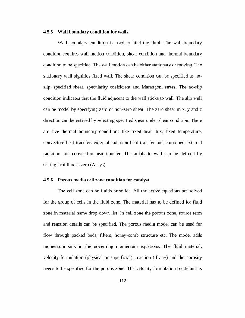
112
4.5.5 Wall boundary condition for walls
Wall boundary condition is used to bind the fluid. The wall boundary
condition requires wall motion condition, shear condition and thermal boundary
condition to be specified. The wall motion can be either stationary or moving. The
stationary wall signifies fixed wall. The shear condition can be specified as no-
slip, specified shear, specularity coefficient and Marangoni stress. The no-slip
condition indicates that the fluid adjacent to the wall sticks to wall. The slip wall
can be model by specifying zero or non-zero shear. The zero shear in x, y and z
direction can be entered by selecting specified shear under shear condition. There
are five thermal boundary conditions like fixed heat flux, fixed temperature,
convective heat transfer, external radiation heat transfer and combined external
radiation and convection heat transfer. The adiabatic wall can be defined by
setting heat flux as zero (Ansys).
4.5.6 Porous media cell zone condition for catalyst
The cell zone can be fluids or solids. All the active equations are solved
for the group of cells in the fluid zone. The material has to be defined for fluid
zone in material name drop down list. In cell zone the porous zone, source term
and reaction details can be specified. The porous media model can be used for
flow through packed beds, filters, honey-comb structure etc. The model adds
momentum sink in the governing momentum equations. The fluid material,
velocity formulation (physical or superficial), reaction (if any) and the porosity
needs to be specified for the porous zone. The velocity formulation by default is

113
set to superficial velocity. The source for heat, mass, momentum, species or other
scalar quantity can be defined under source tab in fluid dialog box. In the reaction
tab if the mechanism contains wall surface reaction then surface to volume ratio
needs to be specified. This value is the surface area of porous wall per unit
volume and can be considered as a measure of catalyst loading (Ansys).
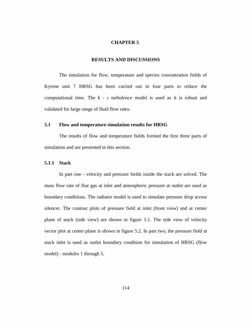
114
CHAPTER 5
RESULTS AND DISCUSSIONS
The simulation for flow, temperature and species concentration fields of
Kyrene unit 7 HRSG has been carried out in four parts to reduce the
computational time. The k - ε turbulence model is used as it is robust and
validated for large range of fluid flow rates.
5.1 Flow and temperature simulation results for HRSG
The results of flow and temperature fields formed the first three parts of
simulation and are presented in this section.
5.1.1 Stack
In part one - velocity and pressure fields inside the stack are solved. The
mass flow rate of flue gas at inlet and atmospheric pressure at outlet are used as
boundary conditions. The radiator model is used to simulate pressure drop across
silencer. The contour plots of pressure field at inlet (front view) and at center
plane of stack (side view) are shown in figure 5.1. The side view of velocity
vector plot at center plane is shown in figure 5.2. In part two, the pressure field at
stack inlet is used as outlet boundary condition for simulation of HRSG (flow
model) - modules 1 through 5.
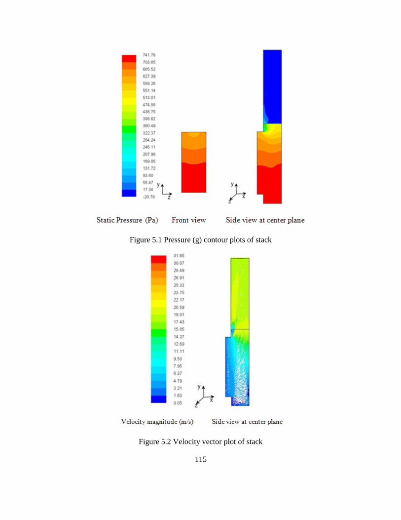
115
Figure 5.1 Pressure (g) contour plots of stack
Figure 5.2 Velocity vector plot of stack
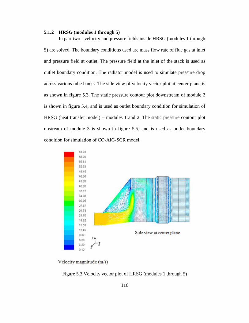
116
5.1.2 HRSG (modules 1 through 5)
In part two - velocity and pressure fields inside HRSG (modules 1 through
5) are solved. The boundary conditions used are mass flow rate of flue gas at inlet
and pressure field at outlet. The pressure field at the inlet of the stack is used as
outlet boundary condition. The radiator model is used to simulate pressure drop
across various tube banks. The side view of velocity vector plot at center plane is
as shown in figure 5.3. The static pressure contour plot downstream of module 2
is shown in figure 5.4, and is used as outlet boundary condition for simulation of
HRSG (heat transfer model) – modules 1 and 2. The static pressure contour plot
upstream of module 3 is shown in figure 5.5, and is used as outlet boundary
condition for simulation of CO-AIG-SCR model.
Figure 5.3 Velocity vector plot of HRSG (modules 1 through 5)
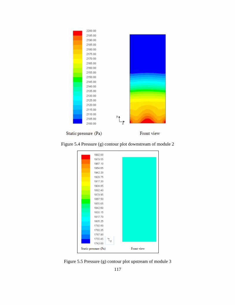
117
Figure 5.4 Pressure (g) contour plot downstream of module 2
Figure 5.5 Pressure (g) contour plot upstream of module 3
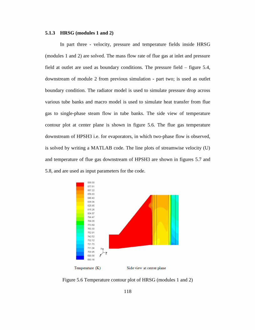
118
5.1.3 HRSG (modules 1 and 2)
In part three - velocity, pressure and temperature fields inside HRSG
(modules 1 and 2) are solved. The mass flow rate of flue gas at inlet and pressure
field at outlet are used as boundary conditions. The pressure field – figure 5.4,
downstream of module 2 from previous simulation - part two; is used as outlet
boundary condition. The radiator model is used to simulate pressure drop across
various tube banks and macro model is used to simulate heat transfer from flue
gas to single-phase steam flow in tube banks. The side view of temperature
contour plot at center plane is shown in figure 5.6. The flue gas temperature
downstream of HPSH3 i.e. for evaporators, in which two-phase flow is observed,
is solved by writing a MATLAB code. The line plots of streamwise velocity (U)
and temperature of flue gas downstream of HPSH3 are shown in figures 5.7 and
5.8, and are used as input parameters for the code.
Figure 5.6 Temperature contour plot of HRSG (modules 1 and 2)
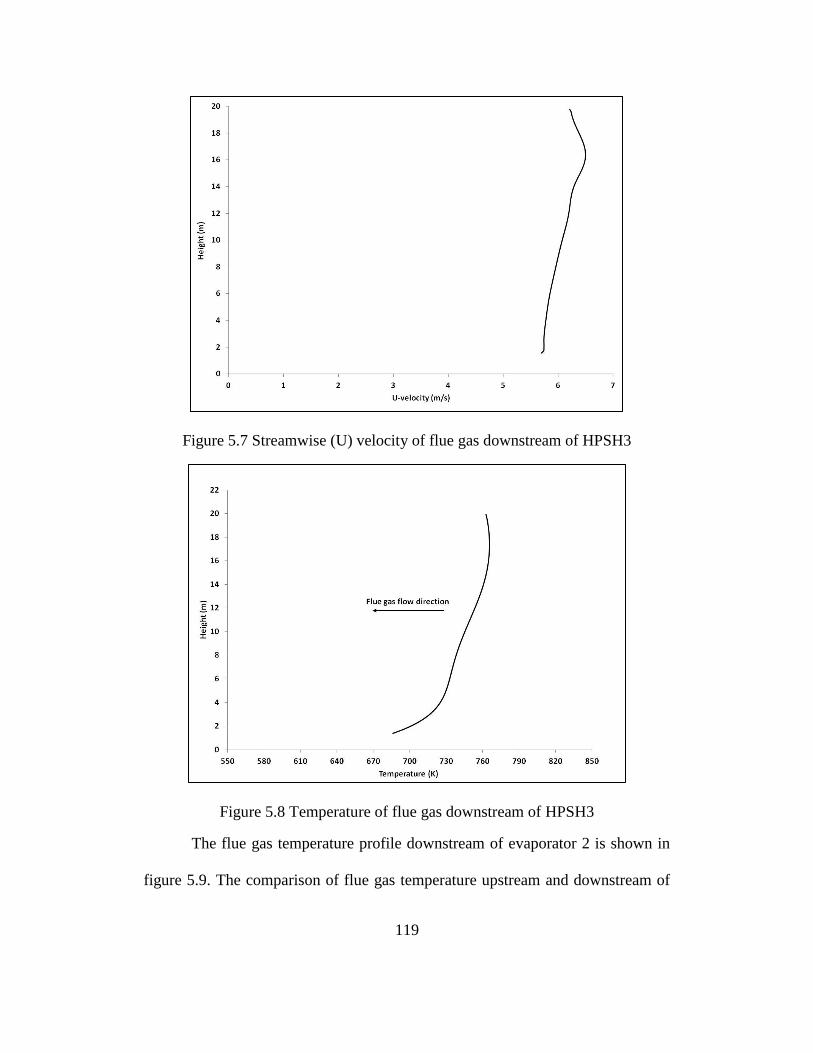
119
Figure 5.7 Streamwise (U) velocity of flue gas downstream of HPSH3
Figure 5.8 Temperature of flue gas downstream of HPSH3
The flue gas temperature profile downstream of evaporator 2 is shown in
figure 5.9. The comparison of flue gas temperature upstream and downstream of
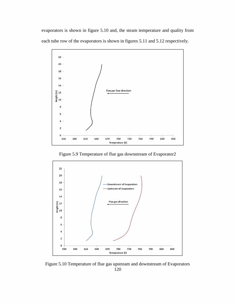
120
evaporators is shown in figure 5.10 and, the steam temperature and quality from
each tube row of the evaporators is shown in figures 5.11 and 5.12 respectively.
Figure 5.9 Temperature of flue gas downstream of Evaporator2
Figure 5.10 Temperature of flue gas upstream and downstream of Evaporators
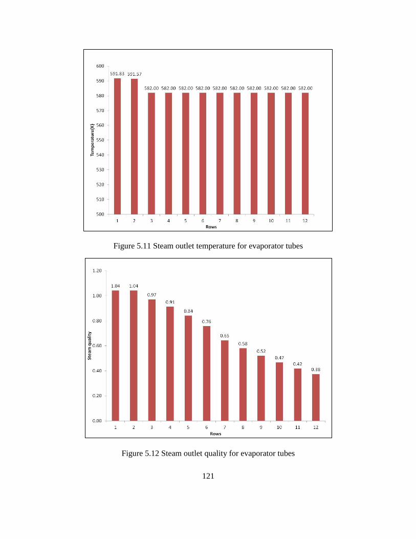
121
Figure 5.11 Steam outlet temperature for evaporator tubes
Figure 5.12 Steam outlet quality for evaporator tubes
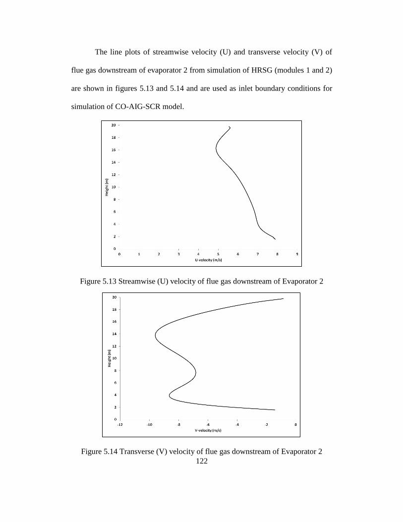
122
The line plots of streamwise velocity (U) and transverse velocity (V) of
flue gas downstream of evaporator 2 from simulation of HRSG (modules 1 and 2)
are shown in figures 5.13 and 5.14 and are used as inlet boundary conditions for
simulation of CO-AIG-SCR model.
Figure 5.13 Streamwise (U) velocity of flue gas downstream of Evaporator 2
Figure 5.14 Transverse (V) velocity of flue gas downstream of Evaporator 2
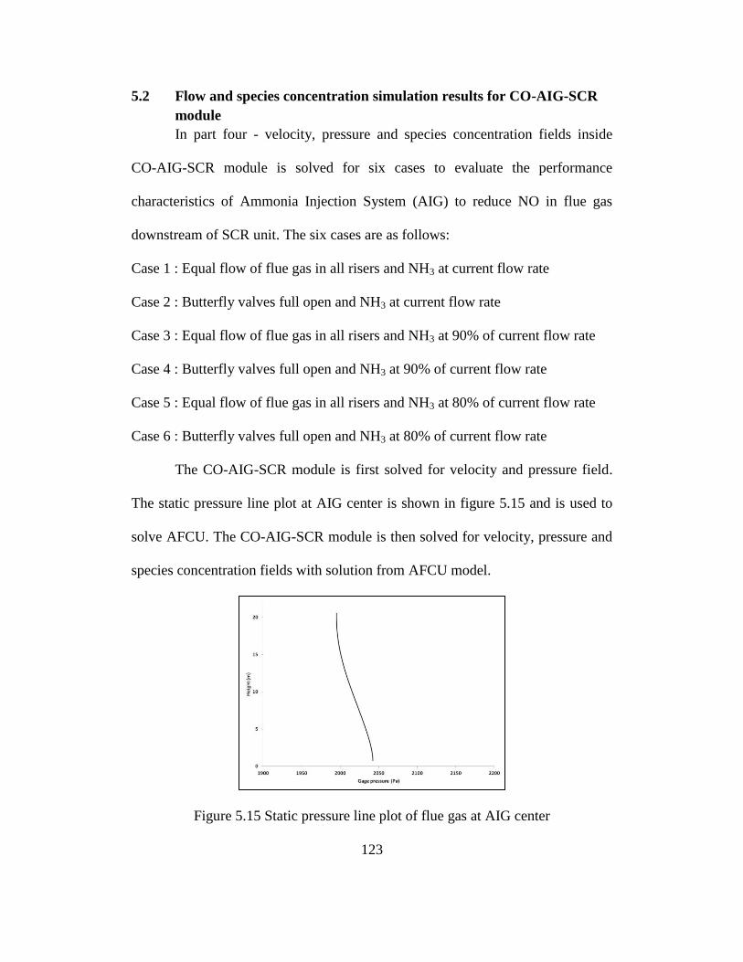
123
5.2 Flow and species concentration simulation results for CO-AIG-SCR
module
In part four - velocity, pressure and species concentration fields inside
CO-AIG-SCR module is solved for six cases to evaluate the performance
characteristics of Ammonia Injection System (AIG) to reduce NO in flue gas
downstream of SCR unit. The six cases are as follows:
Case 1 : Equal flow of flue gas in all risers and NH3 at current flow rate
Case 2 : Butterfly valves full open and NH3 at current flow rate
Case 3 : Equal flow of flue gas in all risers and NH3 at 90% of current flow rate
Case 4 : Butterfly valves full open and NH3 at 90% of current flow rate
Case 5 : Equal flow of flue gas in all risers and NH3 at 80% of current flow rate
Case 6 : Butterfly valves full open and NH3 at 80% of current flow rate
The CO-AIG-SCR module is first solved for velocity and pressure field.
The static pressure line plot at AIG center is shown in figure 5.15 and is used to
solve AFCU. The CO-AIG-SCR module is then solved for velocity, pressure and
species concentration fields with solution from AFCU model.
Figure 5.15 Static pressure line plot of flue gas at AIG center
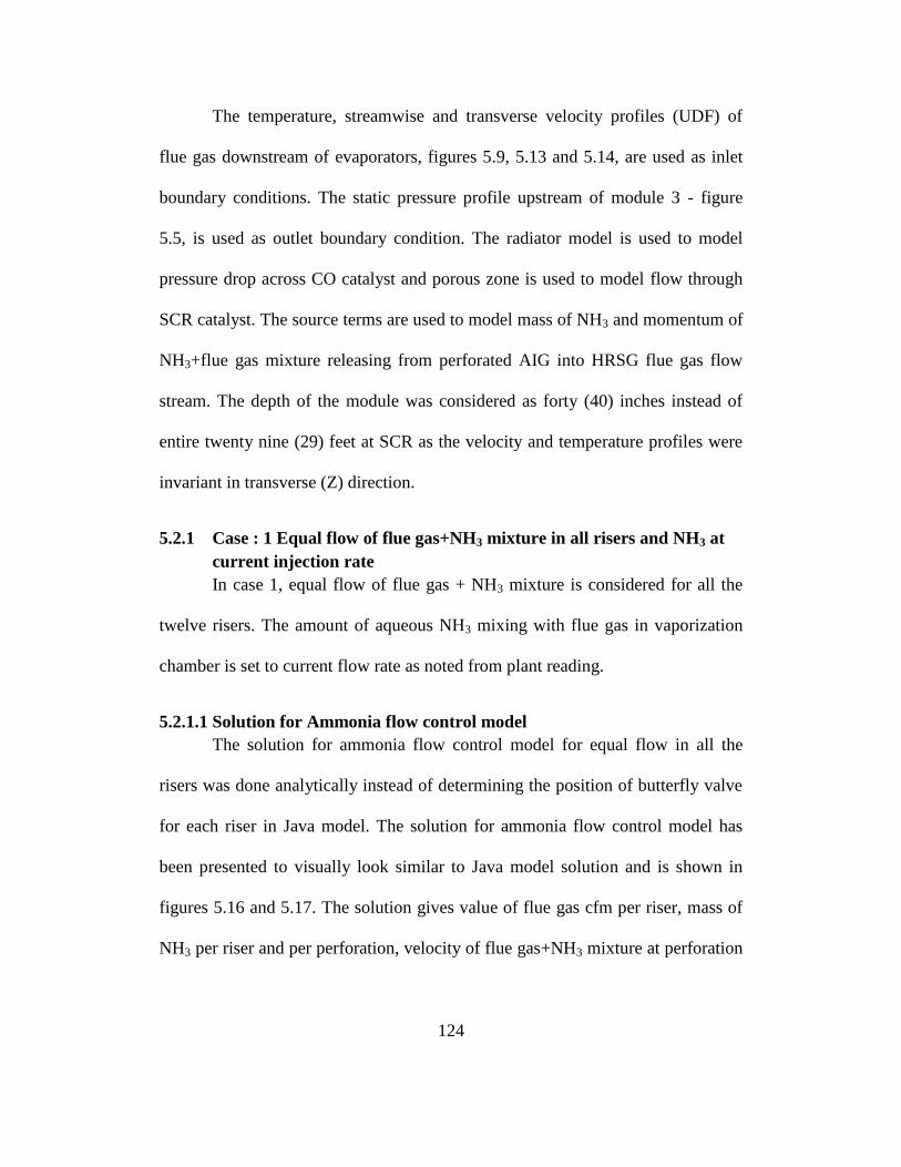
124
The temperature, streamwise and transverse velocity profiles (UDF) of
flue gas downstream of evaporators, figures 5.9, 5.13 and 5.14, are used as inlet
boundary conditions. The static pressure profile upstream of module 3 - figure
5.5, is used as outlet boundary condition. The radiator model is used to model
pressure drop across CO catalyst and porous zone is used to model flow through
SCR catalyst. The source terms are used to model mass of NH3 and momentum of
NH3+flue gas mixture releasing from perforated AIG into HRSG flue gas flow
stream. The depth of the module was considered as forty (40) inches instead of
entire twenty nine (29) feet at SCR as the velocity and temperature profiles were
invariant in transverse (Z) direction.
5.2.1 Case : 1 Equal flow of flue gas+NH3 mixture in all risers and NH3 at
current injection rate
In case 1, equal flow of flue gas + NH3 mixture is considered for all the
twelve risers. The amount of aqueous NH3 mixing with flue gas in vaporization
chamber is set to current flow rate as noted from plant reading.
5.2.1.1 Solution for Ammonia flow control model
The solution for ammonia flow control model for equal flow in all the
risers was done analytically instead of determining the position of butterfly valve
for each riser in Java model. The solution for ammonia flow control model has
been presented to visually look similar to Java model solution and is shown in
figures 5.16 and 5.17. The solution gives value of flue gas cfm per riser, mass of
NH3 per riser and per perforation, velocity of flue gas+NH3 mixture at perforation
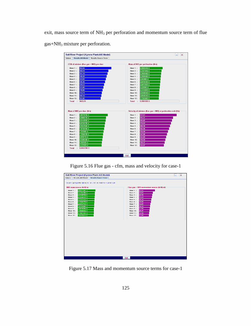
125
exit, mass source term of NH3 per perforation and momentum source term of flue
gas+NH3 mixture per perforation.
Figure 5.16 Flue gas - cfm, mass and velocity for case-1
Figure 5.17 Mass and momentum source terms for case-1
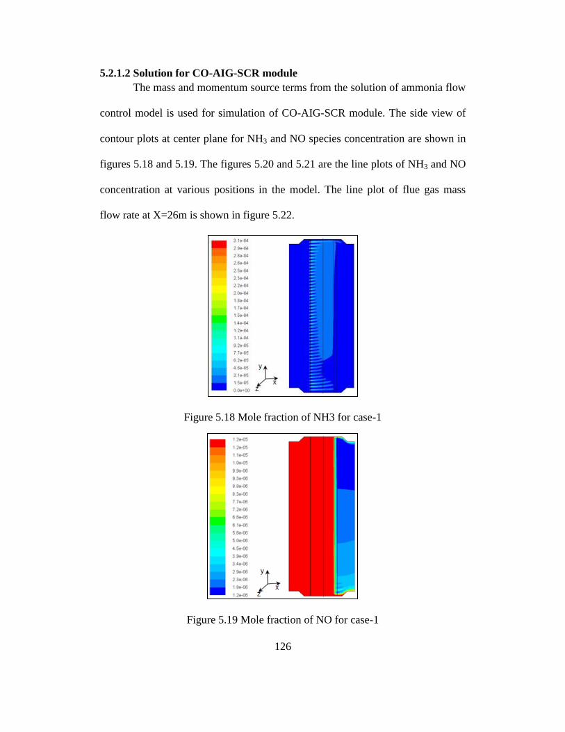
126
5.2.1.2 Solution for CO-AIG-SCR module
The mass and momentum source terms from the solution of ammonia flow
control model is used for simulation of CO-AIG-SCR module. The side view of
contour plots at center plane for NH3 and NO species concentration are shown in
figures 5.18 and 5.19. The figures 5.20 and 5.21 are the line plots of NH3 and NO
concentration at various positions in the model. The line plot of flue gas mass
flow rate at X=26m is shown in figure 5.22.
Figure 5.18 Mole fraction of NH3 for case-1
Figure 5.19 Mole fraction of NO for case-1
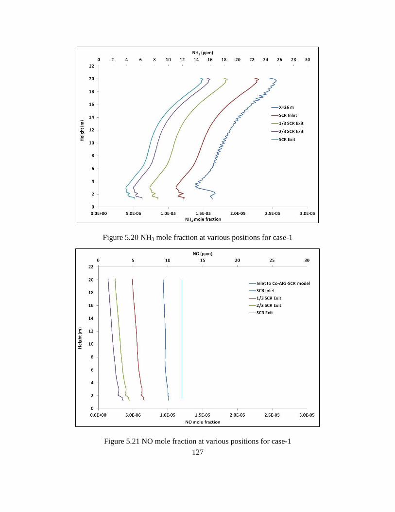
127
Figure 5.20 NH3 mole fraction at various positions for case-1
Figure 5.21 NO mole fraction at various positions for case-1
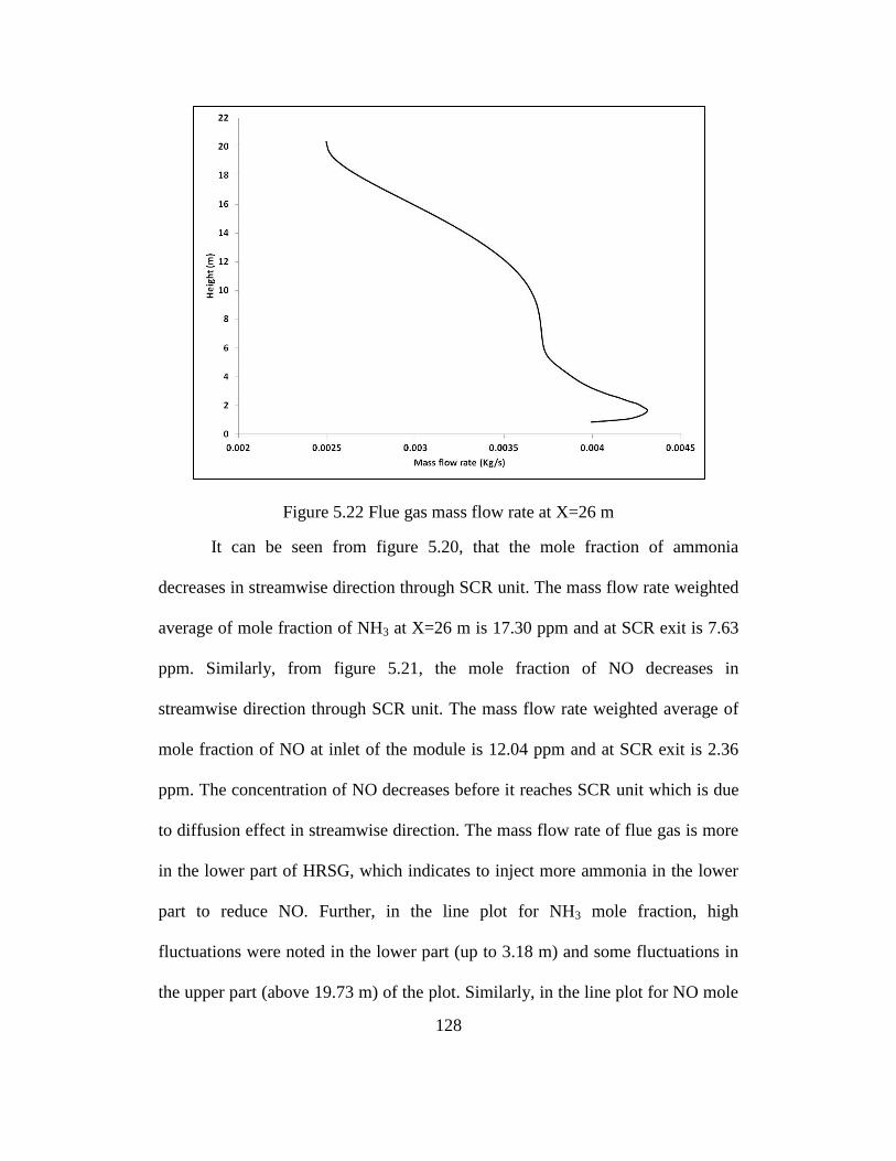
128
Figure 5.22 Flue gas mass flow rate at X=26 m
It can be seen from figure 5.20, that the mole fraction of ammonia
decreases in streamwise direction through SCR unit. The mass flow rate weighted
average of mole fraction of NH3 at X=26 m is 17.30 ppm and at SCR exit is 7.63
ppm. Similarly, from figure 5.21, the mole fraction of NO decreases in
streamwise direction through SCR unit. The mass flow rate weighted average of
mole fraction of NO at inlet of the module is 12.04 ppm and at SCR exit is 2.36
ppm. The concentration of NO decreases before it reaches SCR unit which is due
to diffusion effect in streamwise direction. The mass flow rate of flue gas is more
in the lower part of HRSG, which indicates to inject more ammonia in the lower
part to reduce NO. Further, in the line plot for NH3 mole fraction, high
fluctuations were noted in the lower part (up to 3.18 m) and some fluctuations in
the upper part (above 19.73 m) of the plot. Similarly, in the line plot for NO mole
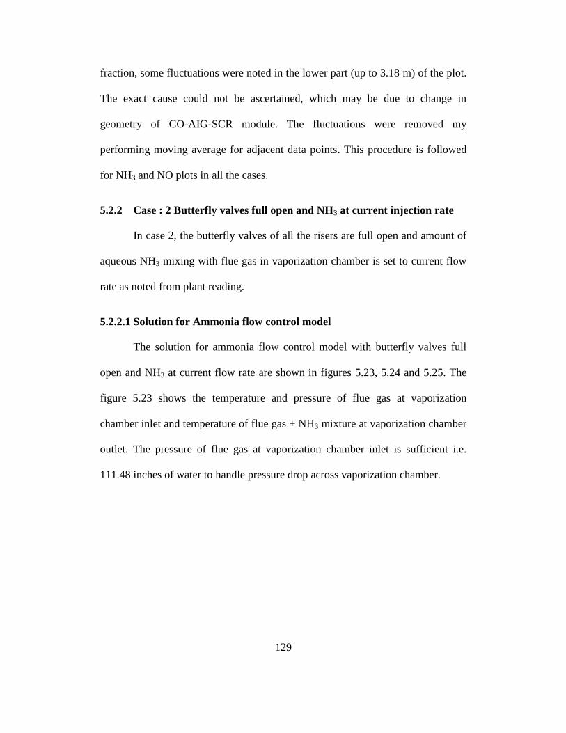
129
fraction, some fluctuations were noted in the lower part (up to 3.18 m) of the plot.
The exact cause could not be ascertained, which may be due to change in
geometry of CO-AIG-SCR module. The fluctuations were removed my
performing moving average for adjacent data points. This procedure is followed
for NH3 and NO plots in all the cases.
5.2.2 Case : 2 Butterfly valves full open and NH3 at current injection rate
In case 2, the butterfly valves of all the risers are full open and amount of
aqueous NH3 mixing with flue gas in vaporization chamber is set to current flow
rate as noted from plant reading.
5.2.2.1 Solution for Ammonia flow control model
The solution for ammonia flow control model with butterfly valves full
open and NH3 at current flow rate are shown in figures 5.23, 5.24 and 5.25. The
figure 5.23 shows the temperature and pressure of flue gas at vaporization
chamber inlet and temperature of flue gas + NH3 mixture at vaporization chamber
outlet. The pressure of flue gas at vaporization chamber inlet is sufficient i.e.
111.48 inches of water to handle pressure drop across vaporization chamber.
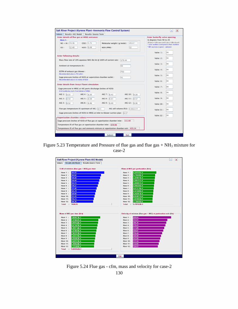
130
Figure 5.23 Temperature and Pressure of flue gas and flue gas + NH3 mixture for
case-2
Figure 5.24 Flue gas - cfm, mass and velocity for case-2
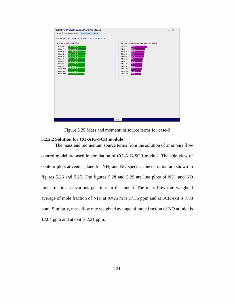
131
Figure 5.25 Mass and momentum source terms for case-2
5.2.2.2 Solution for CO-AIG-SCR module
The mass and momentum source terms from the solution of ammonia flow
control model are used in simulation of CO-AIG-SCR module. The side view of
contour plots at center plane for NH3 and NO species concentration are shown in
figures 5.26 and 5.27. The figures 5.28 and 5.29 are line plots of NH3 and NO
mole fractions at various positions in the model. The mass flow rate weighted
average of mole fraction of NH3 at X=26 m is 17.36 ppm and at SCR exit is 7.53
ppm. Similarly, mass flow rate weighted average of mole fraction of NO at inlet is
12.04 ppm and at exit is 2.21 ppm.
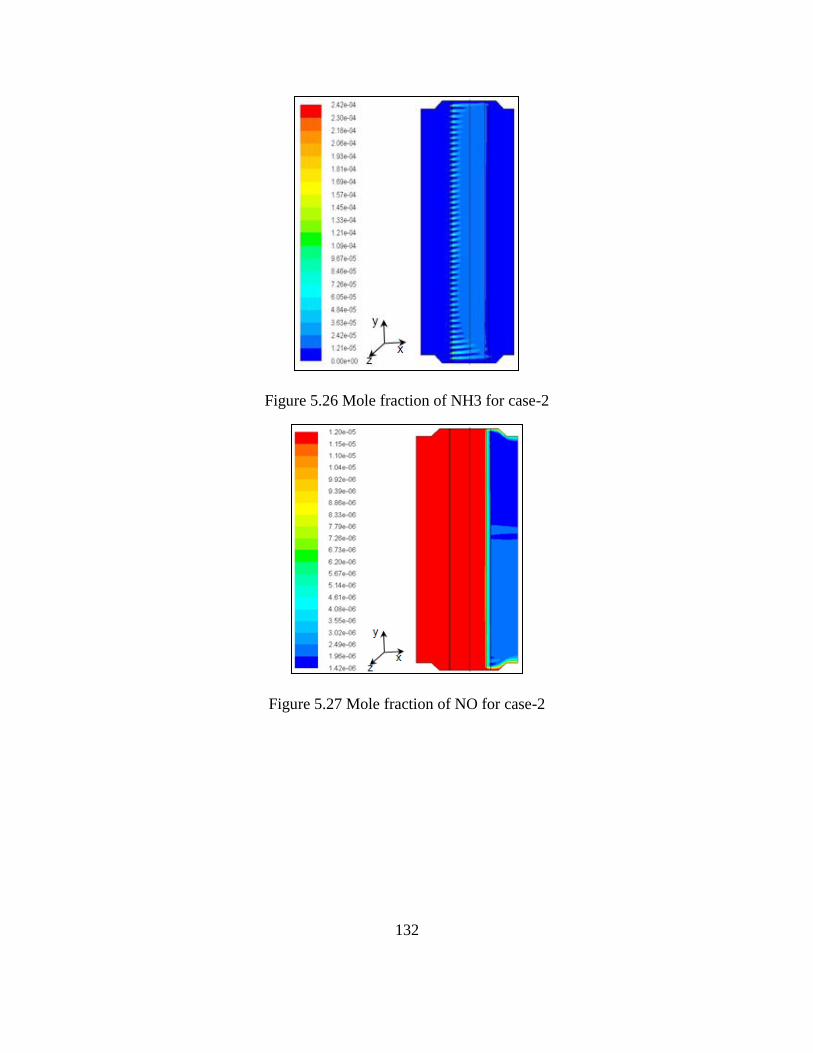
132
Figure 5.26 Mole fraction of NH3 for case-2
Figure 5.27 Mole fraction of NO for case-2
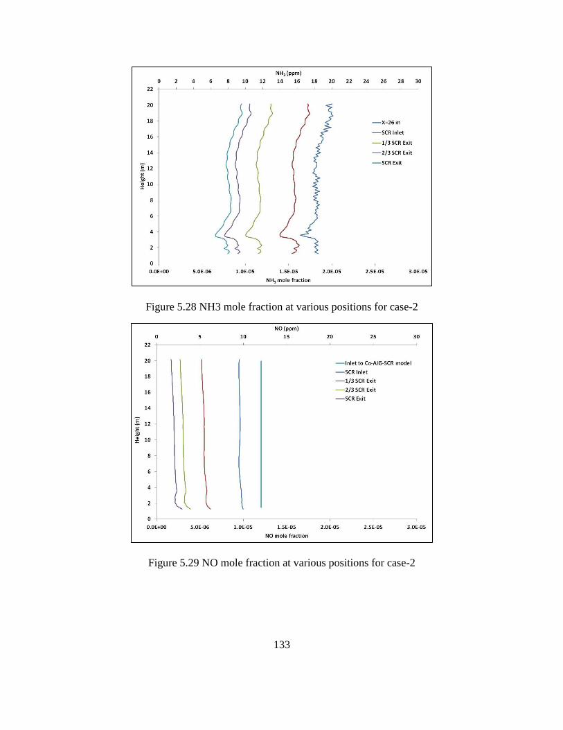
133
Figure 5.28 NH3 mole fraction at various positions for case-2
Figure 5.29 NO mole fraction at various positions for case-2
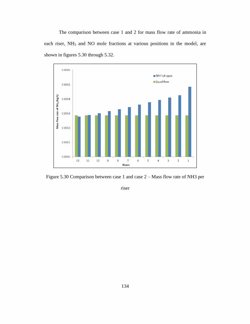
134
The comparison between case 1 and 2 for mass flow rate of ammonia in
each riser, NH3 and NO mole fractions at various positions in the model, are
shown in figures 5.30 through 5.32.
Figure 5.30 Comparison between case 1 and case 2 – Mass flow rate of NH3 per
riser
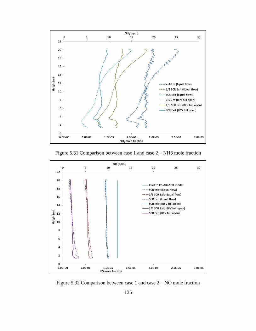
135
Figure 5.31 Comparison between case 1 and case 2 – NH3 mole fraction
Figure 5.32 Comparison between case 1 and case 2 – NO mole fraction
136
The mass flow rate weighted average of mole fraction of NO at exit with
butterfly valves full open is 2.21 ppm and is less compared to case 1 with equal
flow in all the risers.
5.2.3 Case : 3 Equal flow of flue gas+NH3 mixture in all risers and NH3 at
90% of current injection rate
In case 3, equal flow of flue gas + NH3 mixture is considered for all the
twelve risers. The amount of aqueous NH3 mixing with flue gas in vaporization
chamber is set to 90% of current flow rate as noted from plant reading.
5.2.3.1 Solution for Ammonia flow control model
The solution for ammonia flow control model for equal flow in all the
risers was done analytically instead of determining the position of butterfly valve
for each riser in Java model. The solution for ammonia flow control model has
been presented to visually look similar to Java model solution and is shown in
figures 5.33 and 5.34.
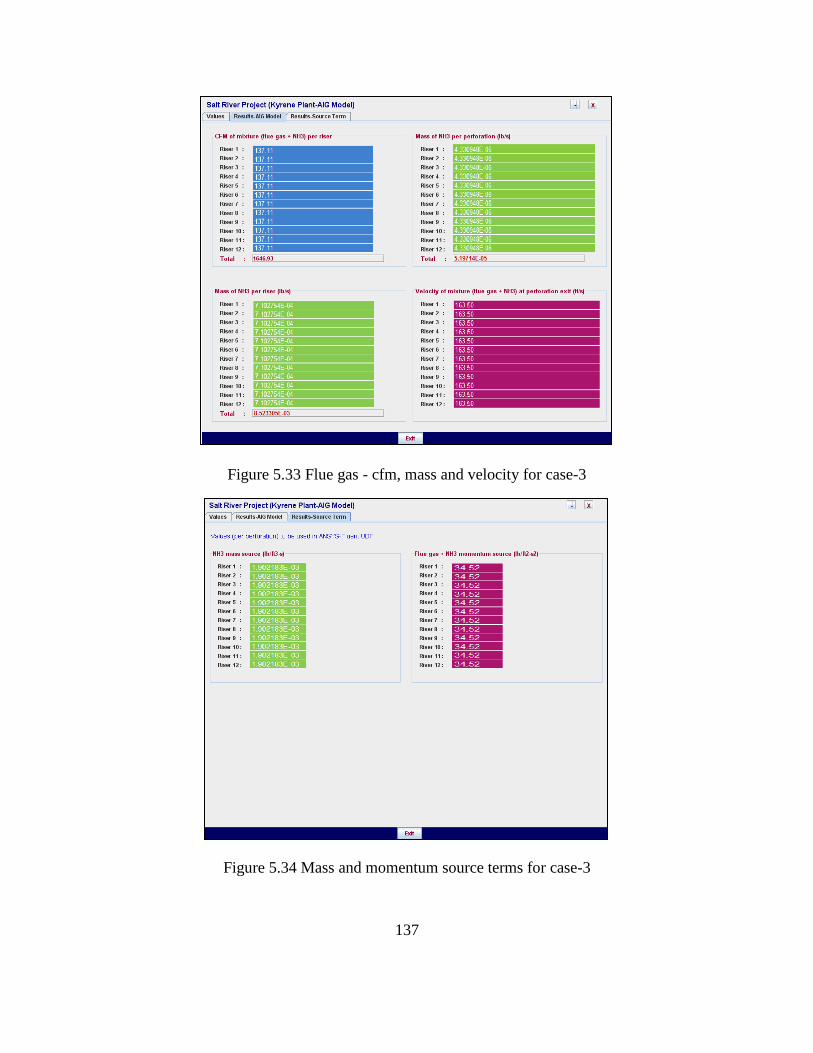
137
Figure 5.33 Flue gas - cfm, mass and velocity for case-3
Figure 5.34 Mass and momentum source terms for case-3
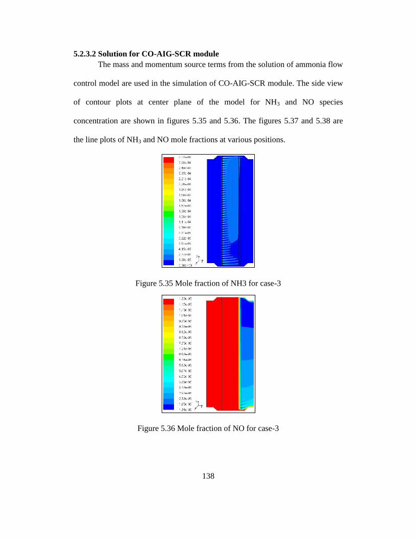
138
5.2.3.2 Solution for CO-AIG-SCR module
The mass and momentum source terms from the solution of ammonia flow
control model are used in the simulation of CO-AIG-SCR module. The side view
of contour plots at center plane of the model for NH3 and NO species
concentration are shown in figures 5.35 and 5.36. The figures 5.37 and 5.38 are
the line plots of NH3 and NO mole fractions at various positions.
Figure 5.35 Mole fraction of NH3 for case-3
Figure 5.36 Mole fraction of NO for case-3
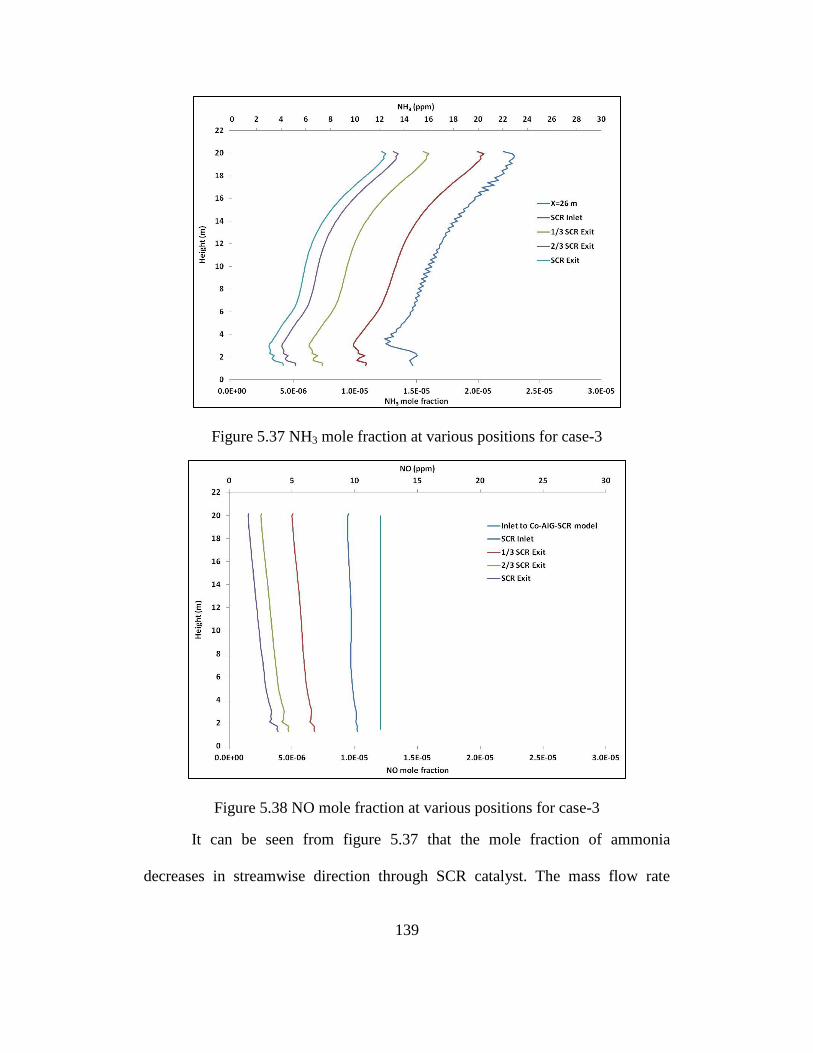
139
Figure 5.37 NH3 mole fraction at various positions for case-3
Figure 5.38 NO mole fraction at various positions for case-3
It can be seen from figure 5.37 that the mole fraction of ammonia
decreases in streamwise direction through SCR catalyst. The mass flow rate
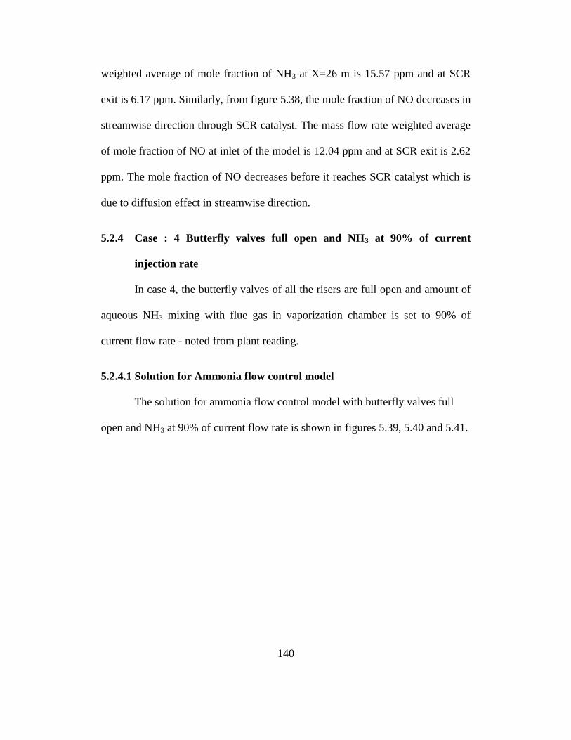
140
weighted average of mole fraction of NH3 at X=26 m is 15.57 ppm and at SCR
exit is 6.17 ppm. Similarly, from figure 5.38, the mole fraction of NO decreases in
streamwise direction through SCR catalyst. The mass flow rate weighted average
of mole fraction of NO at inlet of the model is 12.04 ppm and at SCR exit is 2.62
ppm. The mole fraction of NO decreases before it reaches SCR catalyst which is
due to diffusion effect in streamwise direction.
5.2.4 Case : 4 Butterfly valves full open and NH3 at 90% of current
injection rate
In case 4, the butterfly valves of all the risers are full open and amount of
aqueous NH3 mixing with flue gas in vaporization chamber is set to 90% of
current flow rate - noted from plant reading.
5.2.4.1 Solution for Ammonia flow control model
The solution for ammonia flow control model with butterfly valves full
open and NH3 at 90% of current flow rate is shown in figures 5.39, 5.40 and 5.41.
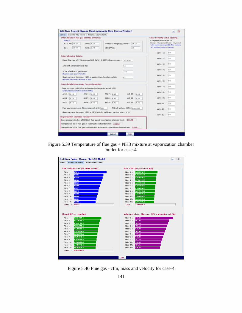
141
Figure 5.39 Temperature of flue gas + NH3 mixture at vaporization chamber
outlet for case-4
Figure 5.40 Flue gas - cfm, mass and velocity for case-4
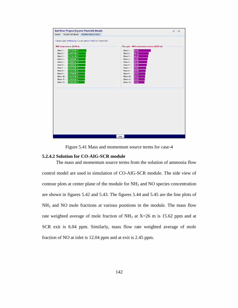
142
Figure 5.41 Mass and momentum source terms for case-4
5.2.4.2 Solution for CO-AIG-SCR module
The mass and momentum source terms from the solution of ammonia flow
control model are used in simulation of CO-AIG-SCR module. The side view of
contour plots at center plane of the module for NH3 and NO species concentration
are shown in figures 5.42 and 5.43. The figures 5.44 and 5.45 are the line plots of
NH3 and NO mole fractions at various positions in the module. The mass flow
rate weighted average of mole fraction of NH3 at X=26 m is 15.62 ppm and at
SCR exit is 6.04 ppm. Similarly, mass flow rate weighted average of mole
fraction of NO at inlet is 12.04 ppm and at exit is 2.45 ppm.
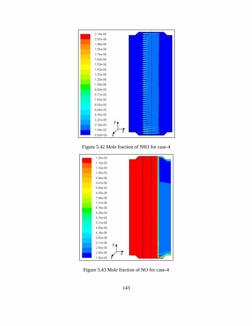
143
Figure 5.42 Mole fraction of NH3 for case-4
Figure 5.43 Mole fraction of NO for case-4
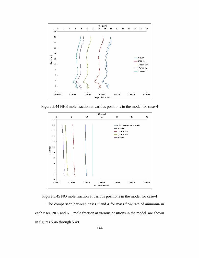
144
Figure 5.44 NH3 mole fraction at various positions in the model for case-4
.
Figure 5.45 NO mole fraction at various positions in the model for case-4
The comparison between cases 3 and 4 for mass flow rate of ammonia in
each riser, NH3 and NO mole fraction at various positions in the model, are shown
in figures 5.46 through 5.48.
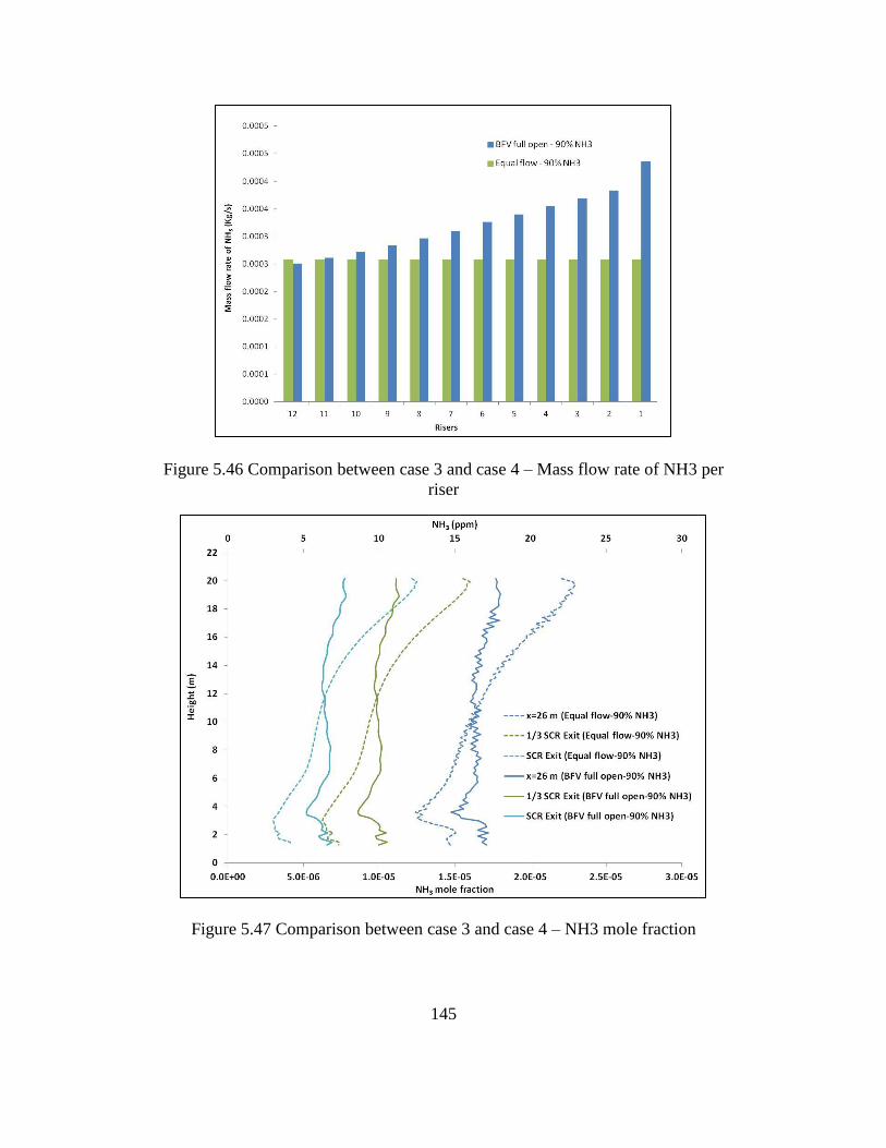
145
Figure 5.46 Comparison between case 3 and case 4 – Mass flow rate of NH3 per
riser
Figure 5.47 Comparison between case 3 and case 4 – NH3 mole fraction
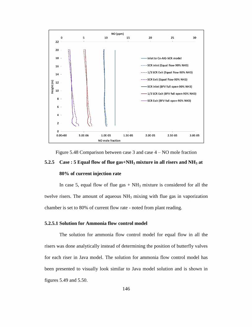
146
Figure 5.48 Comparison between case 3 and case 4 – NO mole fraction
5.2.5 Case : 5 Equal flow of flue gas+NH3 mixture in all risers and NH3 at
80% of current injection rate
In case 5, equal flow of flue gas + NH3 mixture is considered for all the
twelve risers. The amount of aqueous NH3 mixing with flue gas in vaporization
chamber is set to 80% of current flow rate - noted from plant reading.
5.2.5.1 Solution for Ammonia flow control model
The solution for ammonia flow control model for equal flow in all the
risers was done analytically instead of determining the position of butterfly valves
for each riser in Java model. The solution for ammonia flow control model has
been presented to visually look similar to Java model solution and is shown in
figures 5.49 and 5.50.
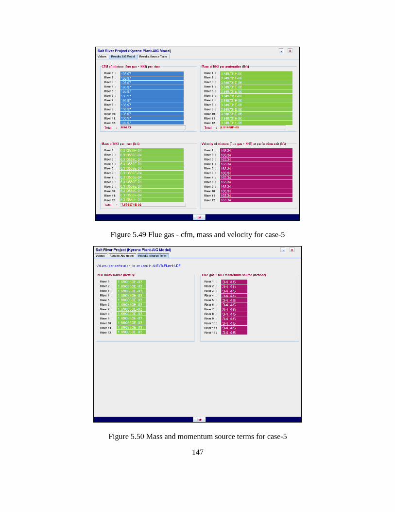
147
Figure 5.49 Flue gas - cfm, mass and velocity for case-5
Figure 5.50 Mass and momentum source terms for case-5
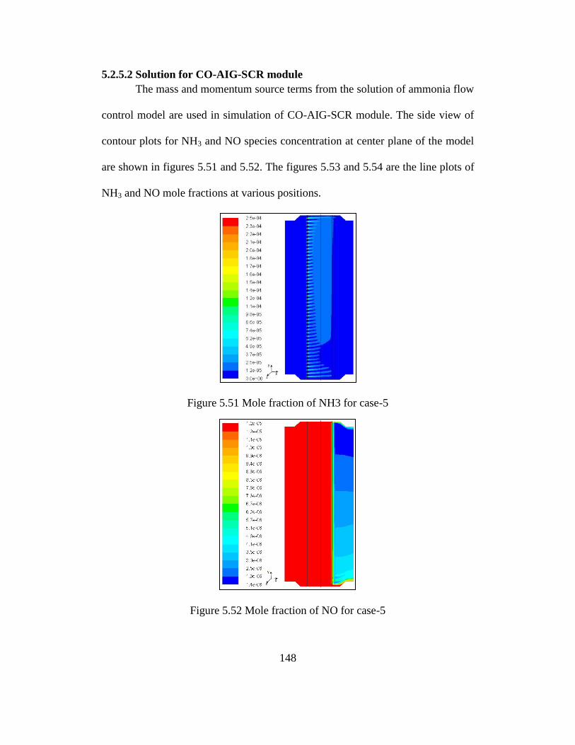
148
5.2.5.2 Solution for CO-AIG-SCR module
The mass and momentum source terms from the solution of ammonia flow
control model are used in simulation of CO-AIG-SCR module. The side view of
contour plots for NH3 and NO species concentration at center plane of the model
are shown in figures 5.51 and 5.52. The figures 5.53 and 5.54 are the line plots of
NH3 and NO mole fractions at various positions.
Figure 5.51 Mole fraction of NH3 for case-5
Figure 5.52 Mole fraction of NO for case-5
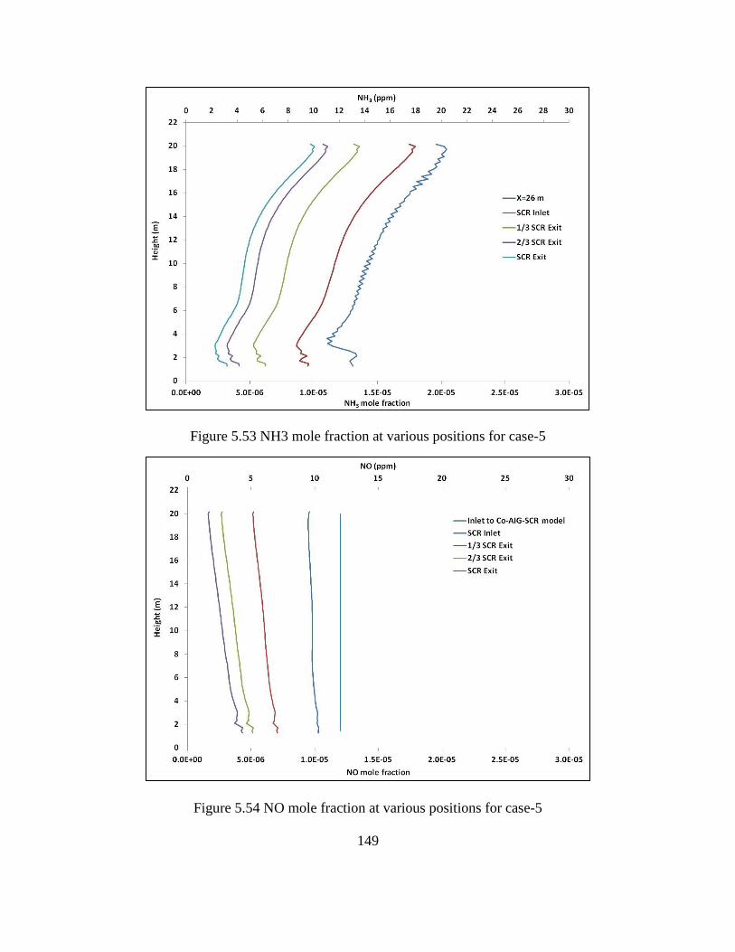
149
Figure 5.53 NH3 mole fraction at various positions for case-5
Figure 5.54 NO mole fraction at various positions for case-5
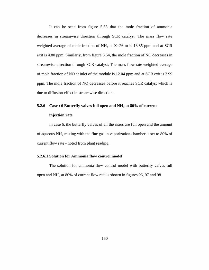
150
It can be seen from figure 5.53 that the mole fraction of ammonia
decreases in streamwise direction through SCR catalyst. The mass flow rate
weighted average of mole fraction of NH3 at X=26 m is 13.85 ppm and at SCR
exit is 4.80 ppm. Similarly, from figure 5.54, the mole fraction of NO decreases in
streamwise direction through SCR catalyst. The mass flow rate weighted average
of mole fraction of NO at inlet of the module is 12.04 ppm and at SCR exit is 2.99
ppm. The mole fraction of NO decreases before it reaches SCR catalyst which is
due to diffusion effect in streamwise direction.
5.2.6 Case : 6 Butterfly valves full open and NH3 at 80% of current
injection rate
In case 6, the butterfly valves of all the risers are full open and the amount
of aqueous NH3 mixing with the flue gas in vaporization chamber is set to 80% of
current flow rate - noted from plant reading.
5.2.6.1 Solution for Ammonia flow control model
The solution for ammonia flow control model with butterfly valves full
open and NH3 at 80% of current flow rate is shown in figures 96, 97 and 98.

151
Figure 5.55 Temperature of flue gas + NH3 mixture at vaporization chamber
outlet for case-6
Figure 5.56 Flue gas - cfm, mass and velocity for case-6
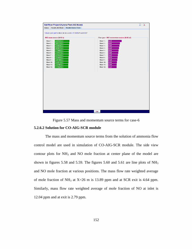
152
Figure 5.57 Mass and momentum source terms for case-6
5.2.6.2 Solution for CO-AIG-SCR module
The mass and momentum source terms from the solution of ammonia flow
control model are used in simulation of CO-AIG-SCR module. The side view
contour plots for NH3 and NO mole fraction at center plane of the model are
shown in figures 5.58 and 5.59. The figures 5.60 and 5.61 are line plots of NH3
and NO mole fraction at various positions. The mass flow rate weighted average
of mole fraction of NH3 at X=26 m is 13.89 ppm and at SCR exit is 4.64 ppm.
Similarly, mass flow rate weighted average of mole fraction of NO at inlet is
12.04 ppm and at exit is 2.79 ppm.

153
Figure 5.58 Mole fraction of NH3 for case-6
Figure 5.59 Mole fraction of NO for case-6
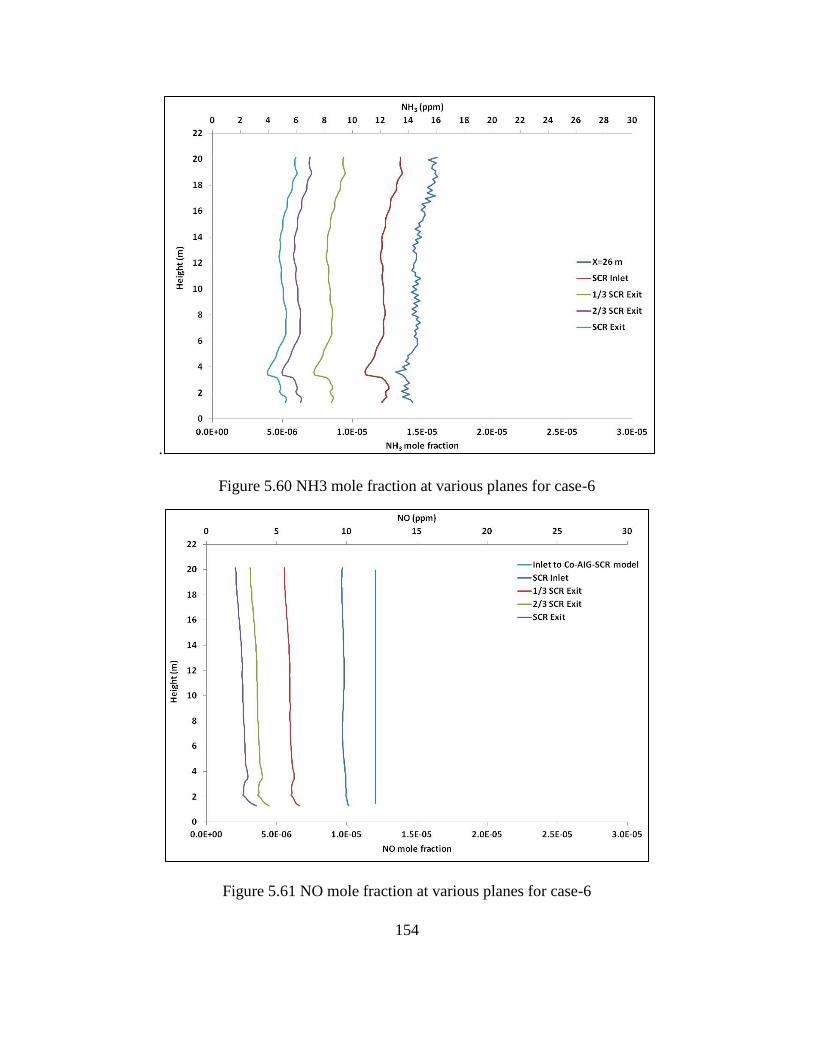
154
.
Figure 5.60 NH3 mole fraction at various planes for case-6
Figure 5.61 NO mole fraction at various planes for case-6
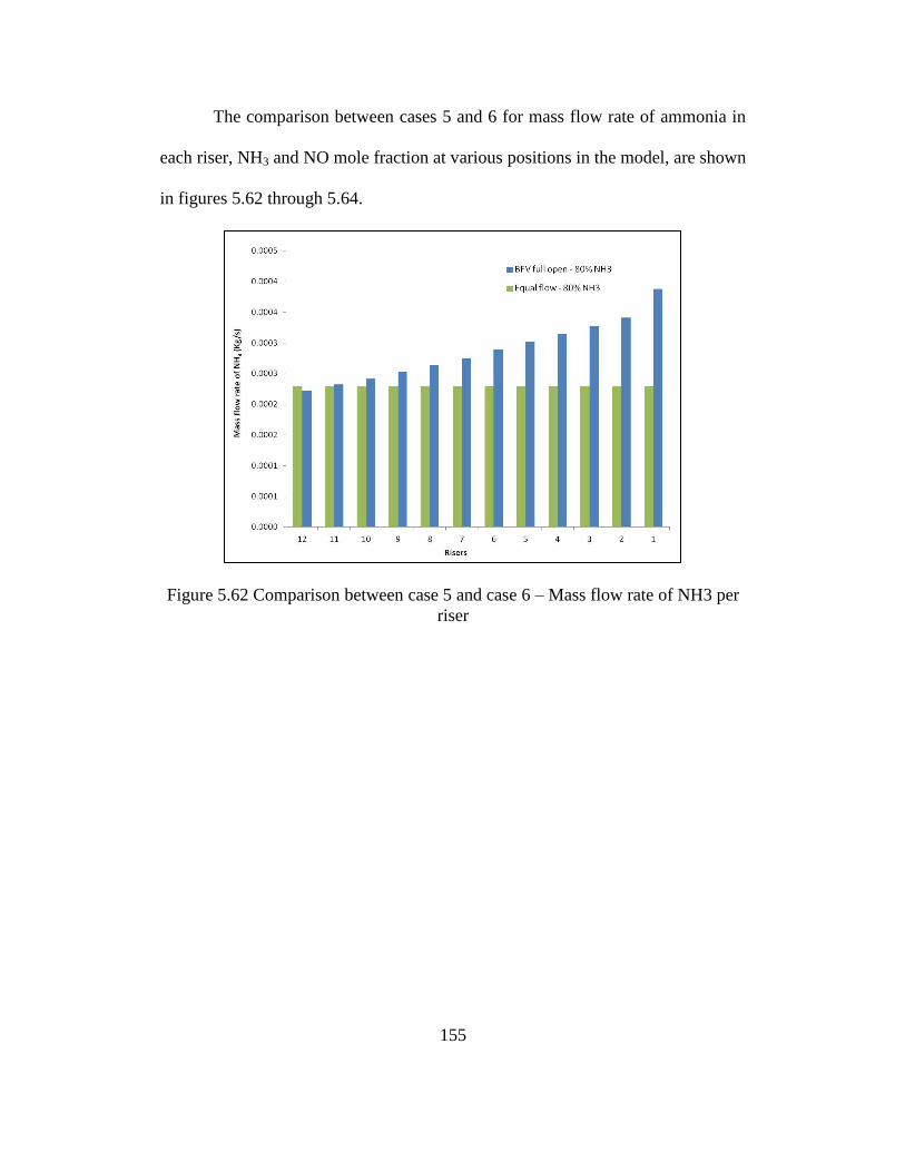
155
The comparison between cases 5 and 6 for mass flow rate of ammonia in
each riser, NH3 and NO mole fraction at various positions in the model, are shown
in figures 5.62 through 5.64.
Figure 5.62 Comparison between case 5 and case 6 – Mass flow rate of NH3 per
riser
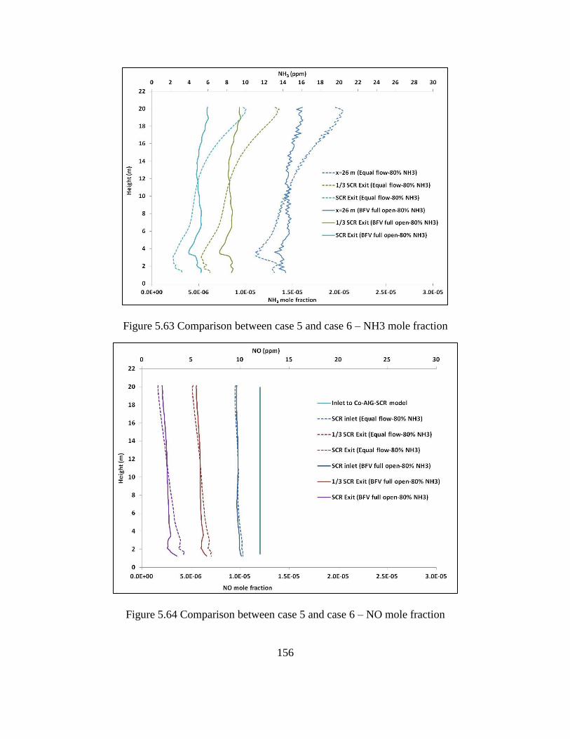
156
Figure 5.63 Comparison between case 5 and case 6 – NH3 mole fraction
Figure 5.64 Comparison between case 5 and case 6 – NO mole fraction
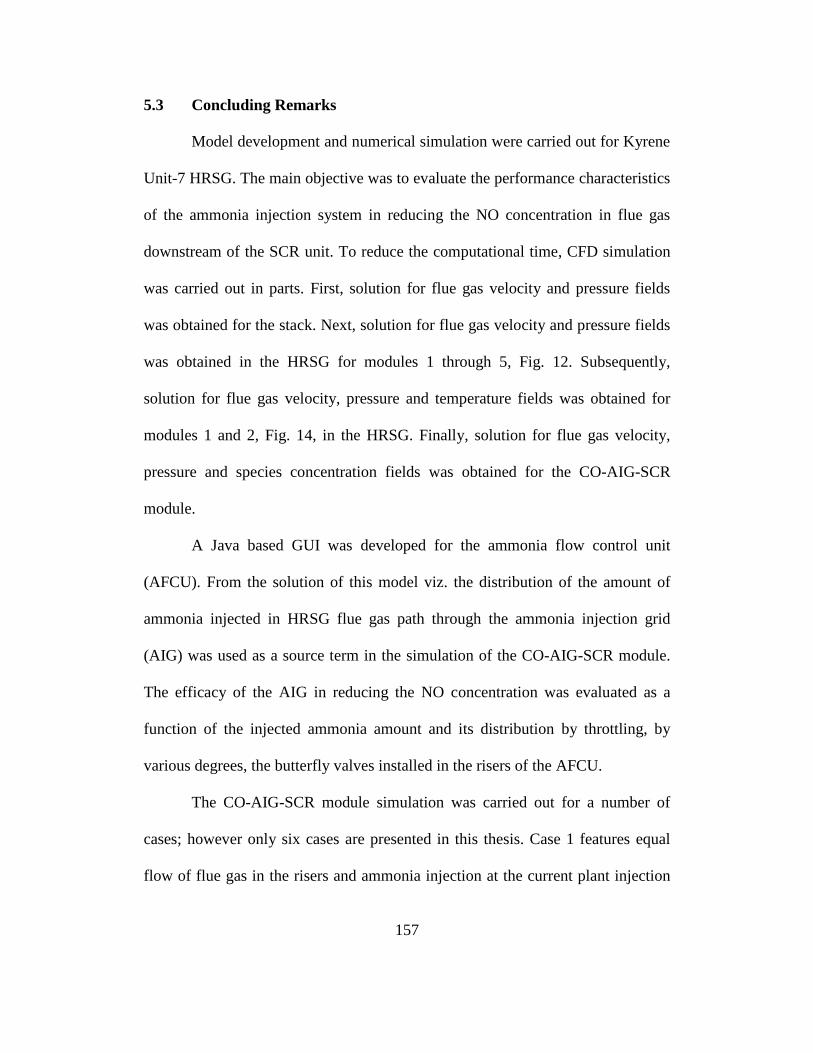
157
5.3 Concluding Remarks
Model development and numerical simulation were carried out for Kyrene
Unit-7 HRSG. The main objective was to evaluate the performance characteristics
of the ammonia injection system in reducing the NO concentration in flue gas
downstream of the SCR unit. To reduce the computational time, CFD simulation
was carried out in parts. First, solution for flue gas velocity and pressure fields
was obtained for the stack. Next, solution for flue gas velocity and pressure fields
was obtained in the HRSG for modules 1 through 5, Fig. 12. Subsequently,
solution for flue gas velocity, pressure and temperature fields was obtained for
modules 1 and 2, Fig. 14, in the HRSG. Finally, solution for flue gas velocity,
pressure and species concentration fields was obtained for the CO-AIG-SCR
module.
A Java based GUI was developed for the ammonia flow control unit
(AFCU). From the solution of this model viz. the distribution of the amount of
ammonia injected in HRSG flue gas path through the ammonia injection grid
(AIG) was used as a source term in the simulation of the CO-AIG-SCR module.
The efficacy of the AIG in reducing the NO concentration was evaluated as a
function of the injected ammonia amount and its distribution by throttling, by
various degrees, the butterfly valves installed in the risers of the AFCU.
The CO-AIG-SCR module simulation was carried out for a number of
cases; however only six cases are presented in this thesis. Case 1 features equal
flow of flue gas in the risers and ammonia injection at the current plant injection
158
rate. In Case 2, the riser butterfly valves are full open and ammonia injection at
current plant injection rate. Case 3 features equal flow of flue gas in the risers and
ammonia injection at 90% of the current plant injection rate. In Case 4, the riser
butterfly valves are full open and ammonia injection at 90% of the current plant
injection rate. Case 5 features equal flow of flue gas in the risers and ammonia
injection at 80% of the current plant injection rate, whereas Case 6 has the riser
butterfly valves full open and ammonia injection at 80% of the current plant
injection rate.
In the current design of the HRSG, the flue gas mass flow rate is higher in
its lower section compared to the upper section, implying that there is more NO
mass flow in the lower section. It was therefore appropriate to introduce more
ammonia in the lower section to reduce NO concentration – this is what happens
when the riser butterfly valves are kept fully open. The mass flow rate-weighted
average values of NO concentration downstream of the SCR unit for cases with
the riser butterfly valves fully open were lower compared to the cases with equal
flow in the risers – thus, the former represents an improvement in the flue gas
quality downstream of SCR unit. For Case 4, the CO-AIG-SCR module
consumed 10% less ammonia while providing acceptable NO concentration
downstream of the SCR.
It should also be noted that the SCR catalyst would be consumed
somewhat more uniformly and the ammonia „slip‟ (ammonia not consumed in the

159
catalytic reaction) would be lower in the “butterfly valves full open” cases,
compared to the corresponding “equal flow in risers” cases.
160
REFERENCES
Ansys Fluent 12.0 - User's Guide. 2009.
Ashrafi-Nik, M. "Thermo hydraulic optimization of the EURISOL DS target".
Paul Scherrer Institute 15th December 2006.
Bruce, E. Larock, Roland, W. Jeppson, Gary, Z. Watters,. (2000). Hydraulics of
pipeline systems.
Bejan, Adrian, and Allan D Kraus. Heat transfer handbook. Hoboken New Jersey:
John Wiley & Sons, Inc, 2003.
Collier, John G. Convective boiling and condensation. Second. Maidenhead:
McGraw-Hill Book Company (UK) Limited, 1972.
Crane, Flow of fluids through valves, fittings and pipe. Technical paper 410 .
Dow, Willard M, & Shreveport, L. A. (1950). The uniform distribution of a fluid
flowing through a perforated pipe. Proceedings of the Semi-annual
meeting of the American Society of Mechanical Engineers St. Louis, Mo.
Flaxbart Edward W (1978). Standards of tubular exchanger manufacturers
association.
Ferziger, J.H., and Milovan Peric. Computational Methods for Fluid Dynamics.
3rd. New York: Springer-Verlag, 1994.
161
Groeneveld, D. C. 1973. Post-Dryout Heat Transfer at Reactor Operating
Conditions. AECL-4513.
Ho Jeong Chae, Soo Tae Choo, Hoon Choi, In-Sik Nam. “Direct use of Kinetic
Parameters for Modeling and Simulation of a Selective Catalytic
Reduction Process”. Ind. Eng. Chem. Res 2000
Idelchik, I. Handbook of hydraulic resistance. 3rd. Boca Raton, Florida: CRC
Press , 1994.
Beeckman, Jean W, and L Louis Hegedus. "Design of Monolith Catalysts for
Power Plant NOx Emission Control." Ind. Eng. Chem. 1991
Kandlikar, S. G. 1990. A General Correlation for Saturated Two-Phase Flow
Boiling Heat Transfer Inside Horizontal and Vertical Tubes. Journal of
Heat Transfer 112:219-228
Martinez. E, Vicente. W, Salinas. M, Soto. G, “Single-phase experimental
analysis of heat transfer in helically finned heat exchanger”. Applied
Thermal Engineering 3rd
November 2008.
Mench, Matthew M. (2008). Fuel cell engines. Hoboken, New Jersey: John Wiley
& Sons, Inc.
Miller, D. S. (1978). Internal flow systems. BHRA Fluid Engineering.
Taliyan, S. S., Roy, D. P., Grover, R. B., Singh, M., & Govindarajan, G. (1995).
An experimental study of the discharge coefficient of pipe perforations.
Proceedings of the Experiments in fluids
162
Versteeg, H. K., and W. Malalasekera. An introduction to computational fluid
dynamics-The finite volume method. Essex: Longman Scientific &
Technical, 1995.
White, Frank. Viscous Fluid Flow. 2nd. New York: McGraw-Hill.
Young, Hugh D., University Physics, 7th Ed., Addison Wesley, 1992.
Jiyuan, Tu. Guan, Yeoh. Chaoqun Heng , and Liu. Computational Fluid
Dynamics - A Practical Approach. 1st. Burlington: Butterworth-
Heinemann, 2008.