MODELING AND ANALYSIS OF ACTUAL …

MODELING AND ANALYSIS OF ACTUAL

EVAPOTRANSPIRATION USING DATA DRIVEN AND

WAVELET TECHNIQUES

A Thesis

Submitted to the College of Graduate Studies and Research

In Partial Fulfillment of the Requirements

for the

Degree of Master of Science

in the

Department of Civil and Geological Engineering

University of Saskatchewan,

Saskatoon, Saskatchewan, Canada

By

Zohreh Izadifar

© Copyright Zohreh Izadifar, June 2010. All rights reserved.

i

PERMISSION TO USE

The author has agreed that the library, University of Saskatchewan, may make

this thesis freely available for inspection. Moreover, the author has agreed that

permission for extensive copying of this thesis for scholarly purposes may be granted by

the professors who supervised the thesis work recorded herein or, in their absence, by

the head of the Department or the Dean of the College in which the thesis work was

done. It is understood that due recognition will be given to the author of this thesis and

to the University of Saskatchewan in any use of the material in this thesis. Copying or

publication or any other use of the thesis for financial gain without approval by the

University of Saskatchewan and the author’s written permission is prohibited.

Requests for permission to copy or to make any other use of material in this

thesis in whole or part should be addresses to:

Head of the Department of Civil and Geological Engineering,

University of Saskatchewan,

57 Campus Drive,

Saskatoon, Saskatchewan,

Canada, S7N 5A9

ii

ABSTRACT

Large-scale mining practices have disturbed many natural watersheds in northern

Alberta, Canada. To restore disturbed landscapes and ecosystems’ functions,

reconstruction strategies have been adopted with the aim of establishing sustainable

reclaimed lands. The success of the reconstruction process depends on the design of

reconstruction strategies, which can be optimized by improving the understanding of the

controlling hydrological processes in the reconstructed watersheds. Evapotranspiration is

one of the important components of the hydrological cycle; its estimation and analysis

are crucial for better assessment of the reconstructed landscape hydrology, and for more

efficient design. The complexity of the evapotranspiration process and its variability in

time and space has imposed some limitations on previously developed

evapotranspiration estimation models. The vast majority of the available models

estimate the rate of potential evapotranspiration, which occurs under unlimited water

supply condition. However, the rate of actual evapotranspiration (AET) depends on the

available soil moisture, which makes its physical modeling more complicated than the

potential evapotranspiration. The main objective of this study is to estimate and analyze

the AET process in a reconstructed landscape.

Data driven techniques can model the process without having a complete

understanding of its physics. In this study, three data driven models; genetic

programming (GP), artificial neural networks (ANNs), and multilinear regression

(MLR), were developed and compared for estimating the hourly eddy covariance (EC)-

measured AET using meteorological variables. The AET was modeled as a function of

five meteorological variables: net radiation (Rn), ground temperature (Tg), air

temperature (Ta), relative humidity (RH), and wind speed (Ws) in a reconstructed

landscape located in northern Alberta, Canada. Several ANN models were evaluated

using two training algorithms of Levenberg-Marquardt and Bayesian regularization. The

GP technique was employed to generate mathematical equations correlating AET to the

five meteorological variables. Furthermore, the available data were statistically analyzed

to obtain MLR models and to identify the meteorological variables that have significant

effect on the evapotranspiration process. The utility of the investigated data driven

iii

models was also compared with that of HYDRUS-1D model, which is a physically

based model that makes use of conventional Penman-Monteith (PM) method for the

prediction of AET. HYDRUS-1D model was examined for estimating AET using

meteorological variables, leaf area index, and soil moisture information. Furthermore,

Wavelet analysis (WA), as a multiresolution signal processing tool, was examined to

improve the understanding of the available time series temporal variations, through

identifying the significant cyclic features, and to explore the possible correlation

between AET and the meteorological signals. WA was used with the purpose of input

determination of AET models, a priori.

The results of this study indicated that all three proposed data driven models

were able to approximate the AET reasonably well; however, GP and MLR models had

better generalization ability than the ANN model. GP models demonstrated that the

complex process of hourly AET can be efficiently modeled as simple semi-linear

functions of few meteorological variables. The results of HYDRUS-1D model exhibited

that a physically based model, such as HYDRUS-1D, might perform on par or even

inferior to the data driven models in terms of the overall prediction accuracy. The

developed equation-based models; GP and MLR, revealed the larger contribution of net

radiation and ground temperature, compared to other variables, to the estimation of

AET. It was also found that the interaction effects of meteorological variables are

important for the AET modeling. The results of wavelet analysis demonstrated the

presence of both small-scale (2 to 8 hours) and larger-scale (e.g. diurnal) cyclic features

in most of the investigated time series. Larger-scale cyclic features were found to be the

dominant source of temporal variations in the AET and most of the meteorological

variables. The results of cross wavelet analysis indicated that the cause and effect

relationship between AET and the meteorological variables might vary based on the

time-scale of variation under consideration. At small time-scales, significant linear

correlations were observed between AET and Rn, RH, and Ws time series, while at larger

time-scales significant linear correlations were observed between AET and Rn, RH, Tg,

and Ta time series.

iv

ACKNOWLEDGMENTS

It is a pleasure to take this chance to thank those who made this thesis possible.

First and foremost I would like to show my deepest gratitude to God for giving me the

opportunity to learn and for His presence and unspeakable generosity, patience, support,

and love.

I am grateful to my supervisor, Dr. Amin Elshorbagy, for his guidance, support,

and opportunities he provided in my graduate experience. His comments and advices

during this research work are sincerely appreciated. I would like to express my gratitude

to my advisory committee members, Dr. Bing C. Si and Dr. Gordon Putz for the

valuable assistance, suggestions, and feedbacks they provided at all levels of my

research project. I also thank Dr. Warren Helgason for taking time to serve as my

external examiner.

This thesis would not have been possible without the financial support of the

Natural Science and Engineering Research Council (NSERC) of Canada, Cumulative

Environmental Management Association (CEMA), and Civil and Geological

engineering, University of Saskatchewan with the scholarship program. Dr. Sean Carey

and Syncrude Canada Ltd. are greatly acknowledged for providing the required data and

cooperating throughout this research work.

I am profoundly indebted to my beloved parents for their unconditional love and

support through my entire life. A special thank you to my dear brother, Mohammad, and

my lovely sisters, Maryam and Zahra, for their support and advices during the hard

times. Appreciation also goes to Dr. Mingbin Huang and Suhad Al Bakri for their kind

assistance in this research.

v

TABLE OF CONTENTS

PERMISSION TO USE .................................................................................................... i

ABSTRACT ................................................................................................................. ii

ACKNOWLEDGMENTS .............................................................................................. iv

TABLE OF CONTENTS ................................................................................................. v

LIST OF TABLES ....................................................................................................... viii

LIST OF FIGURES ........................................................................................................ ix

LIST OF SYMBOLS AND ABBREVIATIONS ........................................................ xii

CHAPTER 1. INTRODUCTION .................................................................................. 1

1.1 Background ......................................................................................................... 1

1.2 Area of Interest .................................................................................................... 2

1.3 Problem Definition .............................................................................................. 4

1.4 Objectives ............................................................................................................ 6

1.5 Scope of the Research ......................................................................................... 7

1.6 Synopsis of the Thesis ....................................................................................... 11

CHAPTER 2. LITERATURE REVIEW .................................................................... 12

2.1 Evapotranspiration ............................................................................................. 12

2.2 Modeling of Evapotranspiration ........................................................................ 13

2.3 Data driven modeling ........................................................................................ 16

2.3.1 Overview .................................................................................................... 16

2.3.2 Artificial Neural Networks (ANNs) ........................................................... 17

2.3.3 Genetic Programming (GP)........................................................................ 21

2.4 Wavelet Analysis (WA) .................................................................................... 24

2.4.1 Overview .................................................................................................... 24

2.4.2 Development History of Wavelet Analysis................................................ 25

2.4.3 Applications of Wavelet Analysis .............................................................. 25

CHAPTER 3. MATERIALS AND METHODS ......................................................... 29

3.1 Overview ........................................................................................................... 29

3.2 Site description .................................................................................................. 29

3.3 Experimental data .............................................................................................. 31


3.4.1 Artificial Neural Networks (ANNs) ........................................................... 36

vi

3.4.2 Genetic programming (GP) ........................................................................ 42

3.4.3 Multilinear regression (MLR) .................................................................... 47

3.5 HYDRUS-1D model ......................................................................................... 49

3.6 Evaluation of models’ Performance .................................................................. 52

3.7 Wavelet Analysis ............................................................................................... 53

3.7.1 Continuous wavelet analysis ...................................................................... 55

3.7.2 Statistical significance test ......................................................................... 59

3.7.3 Cross wavelet analysis ............................................................................... 61

CHAPTER 4. RESULTS AND DISCUSSION ........................................................... 65


4.1.1 Overview .................................................................................................... 65

4.1.2 Data driven modeling data ......................................................................... 66

4.1.3 Artificial Neural Network (ANN) model ................................................... 66

4.1.4 Genetic Programming (GP) model............................................................. 70

4.1.5 Statistical MultiLinear Regression (MLR) model...................................... 76

4.2 Comparison among AET estimation models ..................................................... 81

4.2.1 Conventional model comparison approach ................................................ 81

4.2.2 Rigorous model evaluation approach ......................................................... 83

4.3 Wavelet analysis ................................................................................................ 90

4.3.1 Overview .................................................................................................... 90

4.3.2 Continuous wavelet analysis ...................................................................... 90

4.3.3 Cross wavelet analysis ............................................................................... 98

4.4 Discussion ....................................................................................................... 109

CHAPTER 5. SUMMARY AND CONCLUSION ................................................... 116

5.1 Summary of the study ...................................................................................... 116

5.1.1 Data driven modeling ............................................................................... 117

5.1.2 Wavelet analysis....................................................................................... 118

5.2 Conclusion ....................................................................................................... 119

5.3 Contribution of the research ............................................................................ 120

5.4 Future work ..................................................................................................... 122

5.5 Study limitations .............................................................................................. 123

REFERENCES ............................................................................................................. 124

Appendix A .............................................................................................................. 142

Appendix B .............................................................................................................. 144

vii

Appendix C .............................................................................................................. 146

Appendix D .............................................................................................................. 148

Appendix E .............................................................................................................. 153

viii

LIST OF TABLES

Table 4.1. Statistical Characteristics of data subsets employed for data driven modeling.

.......................................................................................................................................... 66

Table 4.2. Performance statistics of ANN model with 8 hidden neurons for three subsets.

.......................................................................................................................................... 68

Table 4.3. Performance statistics of ANN models with different combinations of inputs.

.......................................................................................................................................... 70

Table 4.4. The best generated GP-based models using various GP parameters for the

cross-validation subset. .................................................................................................... 71

Table 4.5. Performance statistics of the GP-based models using testing subset. ............. 72

Table 4.6. Variables with significant effect on actual evapotranspiration. ...................... 77

Table 4.7. Performance statistics of the MLR models for cross-validation subset. ......... 77

Table 4.8. Performance statistics of different models using testing subset. .................... 82

Table 4.9. General statistical characteristics of errors obtained from different models. . 82

Table 4.10. A comparison among the statistical characteristics of errors obtained from

different models at 0.05 significant level. ........................................................................ 82

Table 4.11. Statistical characteristics of AET data of the years 2005 and 2006. ............. 84

Table 4.12. Performance statistics of different models using 2005 data. ........................ 84

Table 4.13. Performance statistics of different models on the AET values above the 84th

percentile threshold using 2005 data. ............................................................................... 85

Table 4.14. Performance statistics of different models using 2006 data. ........................ 87

Table 4.15. Akiak information criterion and sum squared error of the data driven models

and their required inputs................................................................................................... 88

Table 4.16. Performance statistics of two types of AET models using testing subset of

six-hour data. .................................................................................................................. 112

ix

LIST OF FIGURES

Figure 1.1. Large-scale oil sands mining operation at Mildred Lake Area, Fort

McMurray, Alberta. ........................................................................................................... 2

Figure 1.2. Research Program Framework for Developing a Sustainable Reclamation

Strategy. ............................................................................................................................. 8

Figure 3.1. Location of the reconstructed study area (SWSS). ........................................ 30

Figure 3.2. Soil cover system of the SWSS site. .............................................................. 31

Figure 3.3. Eddy covariance tower at the SWSS site. ...................................................... 34

Figure 3.4. Schematic diagram of an artificial neuron. .................................................... 37

Figure 3.5. Simple configuration of three-layer feed forward ANN (from Fauske, 2006).

.......................................................................................................................................... 38

Figure 3.6. Tree structure symbolic regression GP model for estimation of predictant Y.

.......................................................................................................................................... 43

Figure 3.7. Crossover operation on two selected individuals. ......................................... 44

Figure 3.8. mutation operation on a selected individual. ................................................. 45

Figure 3.9. Examples of mother wavelet functions; (a) Mexican Hat, (b) Morlet, and (c)

Meyer. .............................................................................................................................. 54

Figure 4.1. The influence of number of hidden neurons on the network performance for

two training algorithms using the cross-validation subset: −, Levenberg-Marquardt; ---,

Bayesian-regularization.................................................................................................... 67

Figure 4.2. Visual comparison between the ANN predicted and the observed testing data

of AET: --, observed values; , predicted values. .......................................................... 68

Figure 4.3. Visual comparison between the observed and the GP predicted AET values

of testing data using (a) Eq. (4.1), (b) Eq. (4.2), (c) Eq. (4.3), (d) Eq. (4.4), and (e) Eq.

(4.7): --, observed values; , predicted values. .............................................................. 75

Figure 4.4. Scatter plots of predicted values resulted from (a) MLR model 1 and (b)

MLR model 2 versus measured data using testing subset................................................ 80

Figure 4.5. Probability distribution of the MLR models errors. ...................................... 80

x

Figure 4.6. Visual comparison between the predicted values by (a) model 1 and (b)

model 2 and the observed testing data of AET: --, observed values; , predicted values.

.......................................................................................................................................... 81

Figure 4.7. Probability distribution of the data driven models errors. ............................. 82

Figure 4.8. Scatter plots of predicted actual evapotranspiration (AET) versus observed

AET by (a) ANN, (b) GP (Eq. 4.1), and (c) MLR model using testing subset. ............... 83


AET by (a) ANN, (b) GP (Eq. 4.2), (c) MLR, and (d) HYDRUS model using 2005 data.

.......................................................................................................................................... 86

Figure 4.10. Continuous wavelet power spectrum of hourly time series for the scale

range of 2 to 48 hours; (a) AET, (b) Rn. The thick black contours show the 95%

confidence level against red noise.................................................................................... 91

Figure 4.11. Continuous wavelet power spectrum (top) and time series of hourly AET

(bottom). The thick black contours show the 95% confidence level against red noise. .. 92

Figure 4.12. Continuous wavelet power spectrum (top) and time series of hourly Tg


Figure 4.13. Time series of AET and Tg for a typical time-window of 48 hours. ........... 94

Figure 4.14. Continuous wavelet power spectrum (top) and time series of hourly Ta


Figure 4.15. Continuous wavelet power spectrum (top) and time series of hourly RH


Figure 4.16. Continuous wavelet power spectrum (top) and time series of hourly Rn


Figure 4.17. Continuous wavelet power spectrum (top) and time series of hourly Ws


Figure 4.18. Cross wavelet transform of the AET-Rn time series. The thick black

contours show the 95% confidence level against red noise. Pointing right and left arrows

show in-phase and anti-phase relationship, respectively. ................................................ 99

Figure 4.19. Cross wavelet transform of the AET-RH time series. The thick black


show in-phase and anti-phase relationship, respectively. .............................................. 100

xi

Figure 4.20. Cross wavelet transform of the AET-Ws time series. The thick black



Figure 4.21. Cross wavelet transform of the AET-Tg time series. The thick black



Figure 4.22. Cross wavelet transform of the AET-Ta time series. The thick black



Figure 4.23. Cross wavelet transform of the AET-Ta time series for the scale range of 2

to 48 hours. The thick black contours show the 95% confidence level against red noise.

Pointing right and left arrows show in-phase and anti-phase relationship. ................... 103

Figure 4.24. Cross wavelet transform of the AET and GP-evolved time series by (a) Eq.

(4.20), (b) Eq. (4.21), (c) Eq. (4.22), and (d) Eq. (4.23). The thick black contours show

the 95% confidence level against red noise. Pointing right and left arrows show in-phase.

........................................................................................................................................ 107

Figure 4.25. Visual comparison between the observed and the GP-evolved AET time

series by (a) Eq. (4.20), (b) Eq. (4.21), (c) Eq. (4.22), and (d) Eq. (4.23) over a typical

time-window of 72 hours: --, observed values; , predicted values. ........................... 108

Figure 4.26. Visual comparison of six-hour (day-time) variations of water content (WC),

Rn, Tg, and AET versus time........................................................................................... 111

Figure 4.27. Visual comparison between hourly variations of leaf area index (LAI) and

AET versus time. ............................................................................................................ 113

xii

LIST OF SYMBOLS AND ABBREVIATIONS

AET actual evapotranspiration [mm/h]

b bias [-]

cp specific heat of soil moisture [kJ kg-1

oC

-1]

CWT(η,s) continuous wavelet transform at scale s and time location η [-]

es saturation vapour pressure [kPa],

es-ea vapour pressure deficit [kPa],

ea actual vapour pressure [kPa],

ETo potential evapotranspiration from reference crop [mm h-1

]

f(θrel) soil wetness function [-]

G soil heat flux [MJ m-2

h-1

]

gk gradient of the error function surface [mm/h]

J maximum number of studied scales [-]

k number of observations in AIC formula [-]

Kc crop coefficient [-]

l number of optimized parameters in AIC formula [-]

LAI leaf area index [m2/m

2]

LE latent heat energy [MJ m-2

]

m number of ANN weights [-]

MARE mean absolute relative error [-]

msereg modified error function [mm/h]

n number of independent variables in MLR [-]

N number of instances in the sub dataset under consideration [-]

O observed AET [mm/hr]

mean of observed AET [mm/hr]

P predicted AET [mm/hr]

mean of predicted AET [mm/hr]

Pq Fourier transform of red noise signal [-]

q frequency index

R pearson’s correlation coefficient [fraction]

ra aerodynamic resistance [s m-1

]

xiii

rc crop canopy resistance [s m-1

]

RH relative humidity [fraction]

RH' normalized relative humidity [-]

RMSE root mean squared error [mm/h]

Rn net radiation [MJ h-1

]

R'n normalized net radiation [-]

RSS residual sum of squares [mm2/h

2]

s wavelet scale [hour]

s0 smallest analyzed scale [hour]

SSE summation of squared error [mm2/h

2]

T mean half-hour temperature [oC],

Ta air temperature [oC]

T'a normalized air temperature [-]

Tg ground temperature [oC]

T'g normalized ground temperature [-]

w ANN synaptic weight [-]

wij(k) weight vector at neuron j of layer i of ANN at epoch k [-]

wij(k+1) weight vector at neuron j of layer i of ANN at epoch k+1.[-]

wv vertical wind speed component [ms-1

]

Ws wind speed [ms-1

]

W's normalized wind speed [-]

cross wavelet between time series X and Y at scale s and time location η

[-]

xi discrete time series signal [dimension of the variable under consideration]

X independent variable in MLR [dimension of considered meteorological

variable]

xn red noise time series at time location n [dimension of the associated

variable]

Y dependent variable in MLR [mm/hr]

Yi observed AET [mm/hr]

Yi´ MLR-predicted AET [mm/hr]

Z (p) confidence level at probability p [-]

zn Gaussian white noise [dimension of the associated variable]

α lag-1 autocorrelation coefficient [-]

xiv

αk learning rate [-]

β0 intercept of MLR [-]

βi MLR coefficients [-]

γ performance ratio [-]

γ' psychrometric constant in Penman-Monteith equation [kPa oC

-1]

Δ slope of the vapour pressure curve [kPa oC

-1]

δj scale step size [-]

ε random error in MLR [mm/hr]

η time parameter in Morlet wavelet [-]

θ water content [fraction]

θfc water content at field-capacity of the soil [fraction]

θpwp water content at permanent wilting point [fraction]

θrel relative water content [-]

λ latent heat of vaporization [MJ kg-1

]

λωt Fourier period [hour]

ν degrees of freedom [-]

ρ air density [kg m-3

]

ρv absolute humidity [kg.m-3

]

ρw water density [kg.m-3

]

ζ standard deviation of time series [dimension of the variable under

consideration]

ζ2 variance of the time series [square of considered variable dimension]

η time location.[hour]

χ2 chi-square [-]

ψo(η) mother wavelet function [-]

ψη,s(t) normalized wavelet function at scale s and time location η [-]

ω0 frequency parameter in Morlet wavelet [-]

AET actual evapotranspiration

AI artificial intelligence

AIC akaike’s information criterion

xv

ANNs artificial neural networks

AR [1] lag-1 auto regressive process

ASCE American society of civil engineers

COI cone of influence

CWT continuous wavelet transformation

DWT discrete wavelet transform

EBBR Energy-balance-Bowen-ratio

EC eddy-covariance

EPR evolutionary polynomial regression

ET evapotranspiration

ETc potential evapotranspiration from actual crop

ETo potential evapotranspiration from reference crop

FAO Food and Agricultural Organization

FFNNs feed forward neural networks

GA genetic algorithms

GP genetic programming

LE latent heat flux

MARE mean absolute relative error

MCDA multi-criterion decision analysis

ML machine learning

MLR multilinear regression

Pc crossover probability

Pdf probability distribution function

PET potential evapotranspiration

Pm mutation probability

PM Penman-Monteith

Pr reproduction probability

PT Priestley-Taylor

R Pearson’s correlation coefficient

RBF-ANN radial-basis function neural network

RMSE root mean squared error

RSS residual sum of squares

SMNNs spiking modular neural networks

xvi

SSE summation of squared error

SWSS south west sand storage

WA wavelet analysis

WC water content

WNN wavelet neural network

1

CHAPTER 1. INTRODUCTION

1.1 Background

One of the major human activities that threaten the natural environment is large-

scale surface mining, which put the original ecosystem and hydrology of a local region

at high risk. As a result of these large-scale mining practices, which usually extend to

hundreds of square kilometres of area and hundreds of meters of depth, millions of

tonnes of solid waste are produced (O’Kane et al., 1998) and various functions of natural

watersheds are destroyed. As a solution for this growing concern, many governments

have forced mine operators to adopt reasonable reclamation strategies for the mined

landscapes (Haigh, 2000). Land reclamation is described as the process of restoration of

disturbed landscapes and establishment of sustainable soil-vegetation-water relationship

to achieve land capabilities corresponding to the natural state (Gilley et al., 1977).

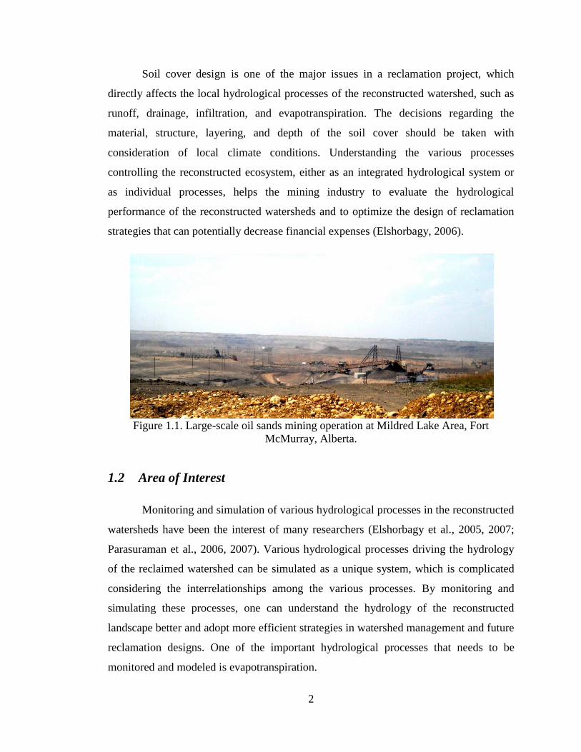
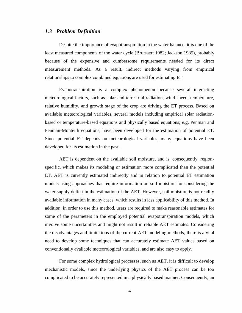
The oil sands industry has disturbed many natural watersheds in northern

Alberta, Canada, where mining activities have been in operation for the extraction of oil

from oil-bearing sands (Fig. 1.1). The oil sands mining practices at Mildred Lake area

near Fort McMurray have affected approximately 1200 km2 of natural environment with

the expectation of expansion to 2000 km2 by 2020 (Carey, 2008). During the mining

process, soil and overburden are removed to gain access to oil bearing deposits. When

the mining practices are over, large-scale open pits resulting from mining operation are

filled and contoured with stockpiled tailing materials and overburden, and then covered

with a topsoil layer to reconstruct the disturbed landscape (Boese, 2003; Elshorbagy et

al., 2005).

The global aim of these reconstruction practices is to establish a sustainable

reclaimed land, which can evolve over time by dynamic interactions between local flora

and fauna and hopefully mimic the natural watershed in the future (Jutla et al., 2006). As

a result, mining industries should adopt reclamation strategies based on sustainable

reclamation principles.

2

Soil cover design is one of the major issues in a reclamation project, which

directly affects the local hydrological processes of the reconstructed watershed, such as

runoff, drainage, infiltration, and evapotranspiration. The decisions regarding the

material, structure, layering, and depth of the soil cover should be taken with

consideration of local climate conditions. Understanding the various processes

controlling the reconstructed ecosystem, either as an integrated hydrological system or

as individual processes, helps the mining industry to evaluate the hydrological

performance of the reconstructed watersheds and to optimize the design of reclamation

strategies that can potentially decrease financial expenses (Elshorbagy, 2006).

Figure 1.1. Large-scale oil sands mining operation at Mildred Lake Area, Fort

McMurray, Alberta.

1.2 Area of Interest

Monitoring and simulation of various hydrological processes in the reconstructed

watersheds have been the interest of many researchers (Elshorbagy et al., 2005, 2007;

Parasuraman et al., 2006, 2007). Various hydrological processes driving the hydrology

of the reclaimed watershed can be simulated as a unique system, which is complicated

considering the interrelationships among the various processes. By monitoring and

simulating these processes, one can understand the hydrology of the reconstructed

landscape better and adopt more efficient strategies in watershed management and future

reclamation designs. One of the important hydrological processes that needs to be

monitored and modeled is evapotranspiration.

3

Evapotranspiration (ET) is a combined term including the transport of water to

the atmosphere in the form of evaporation from the soil surfaces and from the plant

tissues as a result of transpiration. Evapotranspiration plays an important role in the

hydrological cycle and it is considered a major cause of water loss around the world.

Almost 62% of precipitation falls on continents are returned back to the atmosphere

through the evapotranspiration process (Dingman, 2002). In the sub-humid climate of

northern Alberta, ET is the largest annual loss of water (Devito et al., 2005), showing its

vital role in the hydrological system of the reconstructed watersheds.

Evapotranspiration can be conceptually expressed either in the form of potential

or actual evapotranspiration. Potential evapotranspiration (PET) describes the maximum

loss of water from a short green crop under specific climatic conditions when unlimited

water is available. Reference evapotranspiration (ETo), which is a commonly used

concept in engineering and scientific practices, is defined as the rate of

evapotranspiration from a well-defined reference environment (e.g. well-watered short

grass). ETo can be multiplied by a crop-specific coefficient for estimating the crop

evapotranspiration (ETc) (Irmak and Haman, 2003). The actual evapotranspiration

(AET) is the rate at which water is actually removed to the atmosphere from a surface

due to the evapotranspiration process. AET is the preferred form of evapotranspiration in

hydrological analysis because in most cases limited water is available for

evapotranspiration and the actual rate of water loss is of interest.

Accurate assessment of evapotranspiration is of vital importance from different

points of view, such as reliable quantification of hydrological water balance,

hydrological design, water resource planning and management, irrigation system design

and management, and crop yield simulation. In this study actual evapotranspiration as an

individual hydrological process is of interest to be modeled, estimated, and analyzed.

The realization of the evapotranspiration process, which is obtained through

understanding of the temporal variations of AET time series and the meteorological

variables influencing the AET, can be considered as a step forward in the global aim of

better understanding and management of reclaimed watersheds.

4

1.3 Problem Definition

Despite the importance of evapotranspiration in the water balance, it is one of the

least measured components of the water cycle (Brutsaert 1982; Jackson 1985), probably

because of the expensive and cumbersome requirements needed for its direct

measurement methods. As a result, indirect methods varying from empirical

relationships to complex combined equations are used for estimating ET.

Evapotranspiration is a complex phenomenon because several interacting

meteorological factors, such as solar and terrestrial radiation, wind speed, temperature,

relative humidity, and growth stage of the crop are driving the ET process. Based on

available meteorological variables, several models including empirical solar radiation-

based or temperature-based equations and physically based equations; e.g. Penman and

Penman-Monteith equations, have been developed for the estimation of potential ET.

Since potential ET depends on meteorological variables, many equations have been

developed for its estimation in the past.

AET is dependent on the available soil moisture, and is, consequently, region-

specific, which makes its modeling or estimation more complicated than the potential

ET. AET is currently estimated indirectly and in relation to potential ET estimation

models using approaches that require information on soil moisture for considering the

water supply deficit in the estimation of the AET. However, soil moisture is not readily

available information in many cases, which results in less applicability of this method. In

addition, in order to use this method, users are required to make reasonable estimates for

some of the parameters in the employed potential evapotranspiration models, which

involve some uncertainties and might not result in reliable AET estimates. Considering

the disadvantages and limitations of the current AET modeling methods, there is a vital

need to develop some techniques that can accurately estimate AET values based on

conventionally available meteorological variables, and are also easy to apply.

For some complex hydrological processes, such as AET, it is difficult to develop

mechanistic models, since the underlying physics of the AET process can be too

complicated to be accurately represented in a physically based manner. Consequently, an

5

inductive (data driven) modeling approach, which can provide a model to predict and

investigate the process without having a complete understanding of it, can be a useful

tool. Inductive modeling approach is also interesting because of its knowledge discovery

property. Using data driven models, one can extract useful implicit information from a

large collection of data and improve the understanding of the underlying process.

For reconstructed watersheds, it is suggested to perform, at least, five years of

monitoring (Rick, 1995). However, Syncrude Canada Ltd. has changed some of the field

measurement and data collection strategies at some of the reclaimed sites, which shows

the possibility of facing an insufficient monitoring period for modeling purposes. Data

driven models with high generalization abilities can be employed for AET prediction

issues in the reclaimed sites where no AET measurement instrumentation can be made

available.

Among the data driven modeling approaches, standard multilinear regression

(MLR) is a known statistical modeling technique, which has been widely used in the

past for data mining and function estimation problems. Despite the huge development in

the area of data driven modeling, multilinear regression is still popular and being used

for various modeling and model comparison issues. This technique can be examined as a

benchmark modeling method in this study.

Machine learning (ML) techniques are modern data driven modeling methods

that originated from the advances in computer technologies and mathematical

algorithms. These techniques are usually employed for characterizing complicated

systems, which cannot be easily understood, analyzed, and modeled. Artificial neural

networks (ANNs) and genetic programming (GP) are two robust ML techniques, which

apply artificial intelligence for the modeling of complex systems. ANNs are

computational models that can be used for the modeling of complex relationships by

simulating the functional aspects of biological neural networks. GP is an evolutionary-

based technique inspired by the biological evolution to generate computer programs (e.g.

models) for solving a user-defined problem. ANNs and MLR techniques have been

commonly used for modeling of the potential ET process (Kumar et al., 2002; Trajkovic,

2005; Bhakar et al., 2006; Zanetti et al., 2007; Landeras et al., 2008; Chauhan and

6

Shrivastava, 2009), but not considerably for the estimation of AET (Sudheer et al., 2003;

Parasuraman et al., 2006; 2007). GP has been infrequently employed in the

characterization of the ET process, whether AET or potential ET, (Parasuraman et al.,

2007; Parasuraman and Elshorbagy, 2008).

Understanding of AET as well as its correlation with the interacting

meteorological variables can be improved by exploiting the available time series data

and some data mining tools. A new digital signal processing tool, namely wavelet

analysis (WA), has a robust property for providing multiresolution representation of

hydrological time series. Representation of the time series data into time and scale

domains makes it possible to extract useful information about temporal cyclic events

existing in the underlying signal. In addition, the correlation structure of time series data,

in terms of temporal cyclic variations, can be investigated using extensions of wavelet

analysis such as cross wavelet analysis. Temporal variations of AET and meteorological

variables, as well as their correlations, can be examined using wavelet analysis.

1.4 Objectives

This study aims to develop some data driven models and compare their

performances for the estimation of the AET process. It is also of interest to investigate if

data driven models can reveal some information about the AET function and its most

influential variables. Contribution of the meteorological variables to the AET temporal

variations is also of interest and will be examined using wavelet analysis as an approach

to modeling input determination.

The broad aim of this study is to model and analyze the hydrological process of

AET using the data driven techniques and WA. The specific objectives of this study are:

1) To predict actual evapotranspiration using meteorological variables by

developing three different models using ANNs, GP, and statistical multilinear

regression techniques;

7

2) To compare the developed models in terms of predictive accuracy,

generalization ability, structure, and complexity;

3) To identify the most important meteorological variables influencing the AET

process; and

4) To examine the utility of the wavelet analysis in determination of the most

important variables for estimation of AET, prior to the modeling.

1.5 Scope of the Research

The current study fulfills a part of a large research program that aims to develop

a framework to improve understanding of the dynamics of various hydrological

functions driving the hydrology in reconstructed watersheds. The presence of such a

framework seems to be a vital need for efficient and desirable application of an

extensive monitoring program conducted at the experimental reclaimed sites in northern

Alberta, Canada (e.g. south bison hill (SBH) and south west sand storage (SWSS)). The

overall findings of this research program will help the mining industry as well as

reclamation scientists to have a better understanding of the hydrology of the

reconstructed lands and to regulate optimum reclamation strategies that lead to self-

sustainable watersheds. Figure 1.2 (Modified after Jutla, 2006 and Parasuraman, 2007)

shows a diagram of the ongoing overall research program.

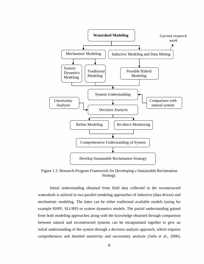
8

Figure 1.2. Research Program Framework for Developing a Sustainable Reclamation

Strategy.

Initial understanding obtained from field data collected in the reconstructed

watersheds is utilized in two parallel modeling approaches of inductive (data driven) and

mechanistic modeling. The latter can be either traditional available models (using for

example HSPF, SLURP) or system dynamics models. The partial understanding gained

from both modeling approaches along with the knowledge obtained through comparison

between natural and reconstructed systems can be encapsulated together to give an

initial understanding of the system through a decision analysis approach, which requires

comprehensive and detailed sensitivity and uncertainty analysis (Jutla et al., 2006).

Watershed Modeling

Mechanistic Modeling Inductive Modeling and Data Mining

System

Dynamics

Modeling

Traditional

Modeling

Possible Hybrid

Modeling

System Understanding

Comprehensive Understanding of System

Re-direct Monitoring Refine Modeling

Decision Analysis

Comparison with

natural system

Uncertainty

Analysis

Current research

work

Develop Sustainable Reclamation Strategy

9

Decision analysis provides some feedback on the already executed monitoring and

modeling program and will be followed by re-directed monitoring and refined modeling

processes to achieve a comprehensive understanding of the reconstructed watershed

systems. Finally, the current reclamation practices can be modified based on the

quantified system understanding to establish a sustainable reclamation strategy. The

framework of the research program comprises the following specific tasks to be

completed (After Jutla, 2006 and Parasuraman, 2007):

Develop a system dynamics watershed simulation model that helps to improve

the understanding of various hydrological functions associated with the

reclaimed watersheds. This task is part of a study running in parallel to the

current study (Keshta et al., 2009);

Adapt some of the available watershed models (e.g. HSPF, SLURP) to the

reconstructed watershed systems and compare the performances of the available

models with the system dynamics model developed in the previous task. This is

to identify the capability of different modeling approaches in capturing the

dynamics of hydrological functions in reconstructed watersheds. A step in this

direction has been recently taken (Keshta and Elshorbagy, 2009);

Conduct inductive modeling and data mining approaches for modeling,

estimation, and analysis of different hydrological processes, individually or as a

system, without considering the physics of the investigated processes. The

current research work attempts to complete this task for one of the important

components of the hydrological cycle in reconstructed watersheds (Fig 1.2).

This study complements earlier attempts by Parasuraman and Elshorbagy

(2008); Parasuraman et al. (2007); and Parasuraman et al. (2006);

Develop inductive and deductive models for natural watersheds and conduct a

comparison between the performances of both watershed modeling approaches

to identify the possible lack of knowledge in the system understanding. This

task also helps to identify the required data for modeling and decision making;

10

Investigate the possibility of combining the advantages of both mechanistic and

inductive modeling approaches for developing the most suitable integrated or

hybrid models for reconstructed watersheds;

Develop a multi-criterion decision analysis (MCDA) tool comprising the

knowledge obtained from different reclamation alternatives for identifying the

most important components influencing the system understanding and

reclamation strategies of reconstructed watersheds. The MCDA technique will

be employed for determining the parameters and hydrological processes that are

highly required to be measured and modeled, and also for identifying the most

suitable modeling approach and the most sustainable reclamation strategies. A

step forward was taken by Elshorbagy (2006); and

Conduct comprehensive uncertainty analysis to determine various uncertainty

components that influence the watershed modeling and decision making

exercise; including the uncertainties associated with the measured variables,

model structures and parameters, and scale and representation of various

hydrological functions.

The current research study is restricted to the inductive modeling and data

mining analysis of actual evapotranspiration function as an individual hydrological

process in reconstructed watersheds, as highlighted in Fig. 1.2. The study is more

focused on the assessment of different data driven modeling techniques and also the

extraction of knowledge from the monitored processes of AET and the meteorological

variables. The current modeling and analysis of the AET process is restricted to an

experimental reconstructed site called south west sand storage (SWSS). The available

data, in this site, are limited to the years of 2005 and 2006, which are used for the

modeling and analysis purposes in this study. The small scale resolution of the data

(hourly) is of interest in this study to be modelled and analyzed. As a result, the

applicability and performance of the proposed models on larger time resolutions are not

discussed here. Since the current study is restricted to one site only, the influence of

vegetation (species and age) and soil structure on the evapotranspiration mechanism are

11

not studied in this thesis. Uncertainty analysis of the modeling exercise will also not be

covered in the present study.

1.6 Synopsis of the Thesis

The rest of this thesis is organized in the following chapters. Chapter 2 provides

the literature review on evapotranspiration modeling methods, development history and

hydrological application of the data driven modeling techniques; ANNs and GP, and

WA. Chapter 3 presents a description of the study area and the experimental data that

were used for modeling and analysis purposes. This chapter also provides a description

of the data driven modeling techniques; ANNs, GP, and MLR, and the WA along with

the associated methodologies for developing the AET prediction models and analysis of

the time series data, respectively. Chapter 4 presents the results and discussions of the

AET modeling, comparative analysis among the various models, and the WA of the

AET and the meteorological time series. In the last chapter, chapter 5, the summary of

the study, conclusions of the results and analysis, research contributions, possible

extensions of the research, and study limitations are provided.

12

CHAPTER 2. LITERATURE REVIEW

Three main techniques, namely, artificial neural networks (ANNs), genetic

programming (GP), and wavelet analysis (WA), were investigated in this study for

modeling and analyzing the challenging process of evapotranspiration. ANNs and GP

were employed as data driven modeling (sometimes called machine learning) techniques

and the wavelet analysis was considered as a signal processing tool. This chapter

provides a brief literature review of these three techniques and their relevant use in

hydrology. In addition, a brief description of the evapotranspiration mechanism and a

literature review on the currently available evapotranspiration models are also presented.

2.1 Evapotranspiration

Evapotranspiration (ET) is the process of returning water back to the atmosphere

through evaporation from open water, soil, and plant surfaces, and transpiration from

plants. Theoretically, evaporation is a diffusive process that follows Fick’s first law and

can be written as a function of vapour pressure deficit (at evaporating surface and

overlying air) and wind speed. Evaporation is accompanied by heat loss from

evaporating surface in the form of latent heat, which can be compensated by radiative or

sensible-heat transfer or by heat transfer from within the evaporating body to the surface

(Dingman, 2002). The rate of latent heat (LE) is related to the evaporation rate using the

latent heat of vaporization and the mass density of water. Physically, the four basic

factors involving the evaporation mechanism include energy availability, water

availability, vapour pressure gradient, wind, and the atmospheric conductance. Any

other parameters that influence the above factors also influence the evaporation process

(McNamara, 2009).

Transpiration is the evaporation of water from the vascular system of the plants

into the atmosphere as a consequence of the photosynthesis process. It involves the

absorption of water from soil through roots and its translocation through the vascular

system of the roots, stem, and branches to the leaves. The water is then moves from the

13

vascular system of the leaf to the walls of stomatals where evaporation takes place.

Water vapour is then released to the atmosphere through the openings of the leaf, called

stomata. Transpiration is limited by energy availability, water availability, humidity,

temperature, ambient CO2 concentration, and wind speed. Plant species come into play

by influencing the leaf conductance and the plant adaptation to water availability

(Dingman, 2002).

When unlimited water is available, the rate of ET is mostly controlled by the

atmospheric conditions, and ET might be near the maximum rate. However, when the

soil water becomes limited, the soil water content starts to control the rate of ET and

may stop the process when the transport of water through the soil becomes critical

(Dingman, 2002). Since in real situations the water is usually not unlimited, the rate of

ET under the limited water supply conditions is said to be the actual rate of

evapotranspiration (AET).

2.2 Modeling of Evapotranspiration

The importance of evapotranspiration (ET) in the water cycle and hydrological

management, in addition to expensive and sensitive measuring equipment, led to

extensive efforts for modeling the ET mechanism. Many methods have been developed,

revised, and proposed for the estimation of ET in different climatic conditions using

different predictor variables. Jensen and Allen (2000) reviewed the evolution of different

types of ET estimation methods. Conventional ET models are basically categorized into

physically based and empirical models. Some examples of the physically based ET

models include the equations developed by Penman (1948), Monteith (1965, 1973),

Shuttleworth and Wallace (1985), and Granger and Gray (1989).

Penman (1948) derived a sound physically based evaporation model by

combining the energy-balance method with the mass-transfer method. The Penman

evaporation model was later modified by Monteith (1965) to take into account the

vegetation surface and the aerodynamic resistance terms, which resulted in the well-

known Penman-Monteith (PM) equation for the estimation of ET. The PM method

14

proved to be superior to about 20 other methods based on the regression analysis of

lysimeter measurements (Jensen et al., 1990). FAO-24 Penman (Doorenbos and Pruitt,

1977) and Kimberly Penman (Wright, 1982, 1996) methods were developed afterwards

following Penman’s theoretical method.

FAO-24 was shown, by different studies such as Jensen et al. (1990), Allen et al.

(1998), and Walter et al. (2001), to lack global validity. The United Nation’s Food and

Agricultural Organization (FAO) recommended a PM-based approach, namely FAO-56

PM (Allen et al., 1998), as the standard method for the estimation of potential

evapotranspiration from a reference surface (ETo) (e.g. grass). The PM model basically

estimates the rate of evapotranspiration from a wet and uniformly vegetated surface

where unlimited water supply is available. The American Society of Civil Engineers

(ASCE, 2004) recommended a Standardized Reference Evapotranspiration (ETo)

Equation on the basis of the ASCE-PM method (Jensen et al., 1990), which is now

generally considered to be the standard technique for the estimation of ETo.

Empirical models were developed with the aim of proposing simpler ET

equations, which require fewer input variables that are also routinely available. Attempts

for empirical modeling of evapotranspiration resulted in various methods: temperature-

based (Thornthwaite, 1948; Blaney and Criddle, 1950; Hargreaves and Samani, 1985),

radiation (and temperature)-based (Priestley and Taylor, 1972; Makkink, 1957; Jensen

and Haise, 1963; Stephens and Stewart, 1963), water budget-based (Guitjens, 1982), and

mass-transfer-based (Harbeck, 1962; Rohwer, 1931). The empirical models have the

advantages of being simple and using a small number of meteorological variables;

however, reasonable estimation of model parameters is required for local applications.

This is considered to be a limitation for the empirical ET prediction models.

In the literature, the vast majority of the studies have been focused on modeling

of the potential evapotranspiration process in which the evaporation occurs from soil and

plant surfaces under no water stress. However, actual evapotranspiration (AET) occurs

under actual conditions of water supply. Quantifying AET has been made possible by

using time- and labour-consuming methods, such as water-balance, energy-balance-

Bowen-ratio (EBBR), and eddy-covariance (EC). EBBR and EC methods are

15

micrometeorological estimation (observation) methods (Droogers, 2000). Since

theoretical modeling of the AET mechanism is complicated, its values are currently

estimated using the available ETo models, crop coefficient (Kc) (as an indication of

actual vegetation), and the information of soil moisture. This approach basically adjusts

the estimated ETo values for the actual investigated plant and soil water condition.

Compared to the ETo, limited studies were observed in the literature, which

investigated the modeling of AET mechanism. Some of these studies are briefly

described here. A simplified method was developed by Slabbers (1980) to predict the

AET based on ETo, crop-dependent critical leaf water potential, and the fraction of

available soil moisture. Poulovassilis et al. (2001) developed a simple semi-empirical

approach for estimating AET using meteorological, crop, and soil data. AET was also

estimated using the relationships developed between AET and pan evaporation

(Bernatowicz et al., 1976; Linacre, 1976; Dolan et al., 1984; Koerselman and Bertman,

1988) and between AET and Penman’s potential evaporation (Koerselman and Bertman,

1988). According to Slabbers (1980), the concept of AET is often limited to the semi-

empirical models (Denmead and Shaw, 1962; Zahner, 1967; Grindley, 1969), which are

subject to several limitations.

Some equation-based ET models have also been adapted for the estimation of

AET, such as Penman-Monteith equation (Monteith, 1973) and the work conducted by

Shuttleworth and Wallace (1985). In the PM method, the model parameters (e.g.

aerodynamic resistance of leaf surface) should be specified for the estimation of AET in

cases where the theoretical assumptions of PM method are not valid (e.g. low soil

moisture conditions). Priestley-Taylor (PT) method (Priestley and Taylor, 1972) was

also adapted for the estimation of AET using an empirical parameter (Pauwels and

Samson, 2006). A strong dependence was found between the empirical parameter of PT

method and the soil moisture condition by Gavin and Agnew (2004). The proposed AET

models mainly require extensive predictor variables, such as meteorological parameters,

soil moisture information, leaf area, and canopy aerodynamic characteristics. The most

encountered problem in the application of the currently available models is the lack of

the required information. According to Poulovassilis et al. (2001), determination of

16

critical parameters (e.g. threshold soil moisture and threshold leaf water potential) is also

a serious obstacle in AET estimation using the available models.

2.3 Data driven modeling

2.3.1 Overview

Improving the predictive ability of hydrological models and the understanding of

hydrological processes are the concern and focus of most hydrologists and modelers

(Lange, 1999). Therefore, extensive studies have been conducted for developing more

reliable and efficient hydrological models. Owing to the recent developments in

computer technologies and new mathematical algorithms, data driven modeling

techniques have been developed as a new approach for simulation and prediction of

various natural and artificial phenomena. These new techniques are of particular interest

in hydrological modeling, which is extensively used for modeling complex and not fully

understood natural processes.

Among the available data driven techniques, which do not require

comprehensive knowledge of the physics of the investigated processes, are ANNs and

GP. ANNs and GP are the two machine learning techniques employed in this study for

the modeling of the AET process. The utility of these techniques for modeling and

predicting various complex processes has been investigated in the literature, and is

briefly reviewed in the following two sections. Furthermore, in this literature review, a

short history of the development of each technique is provided to highlight the long road

each technique has passed through to become as readily applicable as it is today. These

modeling techniques are becoming even more popular with the recent advances in

software/hardware technologies and digital data acquisition (measuring) methods.

17

2.3.2 Artificial Neural Networks (ANNs)

Development history of ANNs

The concept of Artificial Neural Networks (ANNs) was introduced more than 60

years ago in 1943 (McCulloch and Pitts, 1943) when efforts were concentrated on the

understanding of the human brain and simulating its analytical functioning

(Govindaraju, 2000). Since that time ANNs has experienced huge developments through

a three stage evolvement history (Schalkoff, 1997). During the first stage, preliminary

work was conducted on the development of the artificial neuron. This era ended by a 20-

year lull in neural network research caused by the results of Minsky and Papert’s (1969)

work showing the limitations of the preliminary neuron theorem (Jain et al., 1996).

The second phase of ANNs development began with the Hopfield’s (1982) effort

in iterative autoassociable neural networks and the introduction of Hopfield networks

(Govindaraju, 2000). The second era was followed by the discovery (Werbos, 1974) and

the popularization (Rumelhart and McClelland, 1986) of a rigorous ANN training

algorithm, namely back-propagation. Introduction of the back-propagation training

algorithm made a giant forward step in the transition of ANN research into the

applications in a variety of areas. The third stage involved studying the ANN limitations

and generalizations, its combination with other computational techniques (e.g., genetic

algorithm), and the role of hardware advances in the ANN implementations (Dawson

and Wilby, 2001).

Hydrological modeling using ANNs

Increasing numbers of published studies, especially during the last decade, on the

employment and development of ANNs in various fields including hydrological

modeling, indicates their popularity among researchers. ANNs have been increasingly

used in a variety of fields, such as financial management, computer science, various

branches of engineering, control systems, and environmental science (Dawson and

Wilby, 2001). Taylor (1996) wrote a brief discussion on the general application of

18

ANNs, whereas Flood and Kartam (1994, 1997) discoursed on the ANNs application in

solving different civil engineering problems. The hydrology-related literature is the

focus of this section.

The potential of ANNs in environmental science was discussed by Schmuller

(1990) and Maier and Dandy (2001). Some earlier instances of ANNs in the modeling of

hydrological systems were proposed by Daniel (1991). ASCE (2000a, b) presented a

detailed review on the various applications of ANNs in hydrology. Some examples of

hydrological studies that investigated the potential of ANNs in the modeling of different

hydrological processes include: rainfall-runoff modeling (Zhu et al.,1994; French et al.,

1992; Minnes and Hall 1996; Tokar and Johnson 1999; Elshorbagy et al., 2000; Dawson

and Wilby, 2001; Birikundavy et al., 2002; Campolo et al., 2003; Huang et al., 2004;

Riad et al., 2004; Hettiarachchi et al., 2005; Senthil Kumar et al., 2005), stream flow

modeling (Kang et al., 1993; Karunanithi et al.,1994; Poff et al., 1996; Muttiah et al.,

1997; Elshorbagy et al., 2002), water quality modeling (Maier and Dandy 1996; Rogers

1992; Rogers and Dowla 1994; Starrett et al., 1996; Hutton et al., 1996), river stage

forecasting (Lachtermacher and Fuller, 1994; Thirumalaian and Deo, 1998; Campolo et

al., 1999), characterization of ground water (Aziz and Wong, 1992; Ranjithan et al.,

1993; Rizzo and Dougherty, 1994; Yang et al., 1997), estimation of precipitation

(French et al, 1992; Tohma and Igata, 1994; Hsu et al., 1996, 1997; Kuligowski and

Barros, 1998), and estimation of soil moisture content (Elshorbagy and Parasuraman,

2008). In hydraulic engineering, ANNs have been employed for the prediction of

sediment load (Abrahart and White, 2001; Nagy et al., 2002; Yitian and Gu, 2003;

Bhattacharya et al., 2005) and studying flood wave propagation (Dartus et al., 1993).

Despite the large number of studies which have been conducted on different

hydrological problems, few applications of ANNs can be found in the area of

evapotranspiration, and especially, actual evapotranspiration. Kumar et al. (2002)

developed an ANN model for the prediction of reference evapotranspiration (ETo) and

compared its performance with that of a conventional method (Penman-Monteith

equation) to examine the capabilities of ANNs in ETo prediction compared to the PM

method. The results of the study showed that the ANN model can predict ETo better than

19

the conventional method for the considered local case study. Jothiprakash et al. (2002)

investigated the capability of ANNs for the estimation of ETo using the daily

meteorological variables. It was found that the results of ANN models were in good

agreement with those of FAO-modified Penman method, and that four basic

meteorological variables were sufficient for remarkably accurate estimation of ETo using

ANNs. Trajkovic et al. (2003) developed a radial-basis function type neural network

(RBF-ANN) model for the prediction of ETo. Trajkovic (2005) examined the reliability

of RBF-ANNs as well as three other calibrated temperature-based approaches for the

estimation of ETo. The results confirmed the efficiency of the temperature-based RBF-

ANN model for the prediction of ETo. The utility of ANNs for the estimation of

reference and crop evapotranspiration (ETc) of wheat crop was examined by Bhakar et

al. (2006) and it was revealed that the ANN model was suitable for the prediction of ETo

and ETc. Zanetti et al. (2007) found that by using ANNs, it was possible to estimate ETo

just as a function of maximum and minimum air temperature. The results of a study

conducted by Jain et al. (2008) indicated that ANNs can efficiently estimate ETo from

the limited meteorological variables of temperature and radiation only.

The degree of influence of each of the meteorological variables; wind speed,

solar radiation, relative humidity, air and soil temperature, on the estimation of daily

ETo, and the performance of ANNs compared to those of Penman, Hargreaves, and

multilinear regression (MLR) methods were investigated by Kisi (2006). The study

concluded that the ANN model trained by Levenberg-Marquardt algorithm was superior

to the MLR, Penman, and Hargreaves method. Also, the input combination of wind

speed, solar radiation, relative humidity, and air temperature resulted in the best

performance statistics.

Landeras et al. (2008) developed seven ANNs with different input combinations

and then compared ANNs to locally calibrated empirical and semi-empirical equations

of ETo. Their proposed ANNs performed better than the locally calibrated equations

particularly in situations where appropriate meteorological inputs were lacking. Wang et

al. (2008) employed the capability of ANNs for the prediction of ETo with a limited

meteorological dataset of minimum and maximum air temperature. It was observed that

20

ANN predictions were more accurate than those of the local reference model,

Hargreaves, and Blaney-Criddle method in a semiarid area. Kumar et al. (2008)

developed several ANNs-based ETo models, corresponding to the best ranking

conventional ETo estimation methods, and compared the results with FAO-56 PM ETo

estimation model. The ANN models were consistent with the non-ideal condition of data

availability and predicted ETo values with better closeness to the FAO-56 PM ETo than

the conventional methods.

Dai et al. (2009) investigated the predictive ability of ANNs for the prediction of

ETo in arid, semi-arid, and sub-humid areas of Mongolia, China, and conducted a

comparison between the estimated ETo values from ANNs and MLR. The results

showed that regional ETo can be satisfactorily estimated using ANN models and

conventional meteorological variables. The study also demonstrated that ANNs modeled

ETo better than MLR. Chauhan and Shrivastava (2009) investigated the climatic based

methods as well as ANNs to identify the approach that estimates the closest ETo to the

standard PM ETo. It was found that ANN model can perform better than the climatic

based models and is able to estimate ETo by using only maximum and minimum

temperatures.

In the majority of the conducted studies, researchers have focused on the

modeling of potential and reference crop evapotranspiration but not actual

evapotranspiration (AET). To the knowledge of the author, the only publications

reporting the application of ANNs for the modeling of AET include the studies

conducted by Sudheer et al. (2003) and Parasuraman et al. (2006; 2007). Sudheer et al.

(2003) estimated the lysimeter-measured AET of rice crop using RBF-ANNs. The

results demonstrated that ANNs can successfully estimate the AET.

Parasuraman et al. (2006) developed spiking modular neural networks (SMNNs)

for modeling the dynamics of EC-measured hourly latent heat flux. The results

demonstrated that although the SMNNs are computationally intensive, they can perform

better than regular feed forward neural networks (FFNNs) in modeling evaporation flux.

Parasuraman et al. (2007) developed a regular three-layered FFNN model for the

estimation of EC-measured hourly AET as a function of net radiation, ground

21

temperature, air temperature, wind speed, and relative humidity. Their results indicated

that the ANN model performed better than the currently used PM method in northern

Alberta, Canada.

2.3.3 Genetic Programming (GP)

Development history of GP

The origins of evolutionary computation traced back to the late 1950’s (Box,

1957; Friedberg, 1958; Friedberg et al., 1959; Bremermann, 1962) when it was proposed

for the first time and then remained unknown for almost three decades. Fundamental

works (Holland, 1962; Fogel, 1962; Rechenberg, 1965; schwefel, 1968), conducted

during the 1970’s, started to change the face of this computational approach to an

adaptable and well-suited problem solving tool in the scientific and economic fields

(Back et al., 1997). Genetic algorithm (GA) was first introduced by Holland (1962;

1975; Holland and Reitman, 1978) and then studied and developed by several scientists

(De Jong, 1975, 1987; Goldberg, 1985, 1989; Grefenstette, 1986; Koza, 1989; Davis,

1991; Goldberg et al., 1993; Forrest and Mitchell, 1993; Mitchell, 1996). Genetic

programming (GP), as an extension of GA, was first recognized as a different and new

development in the world of evolutionary algorithms in the seminal monograph of Koza

(1992). In his book, problem solving using GP and evolving tree-like structure solutions

were precisely described.

Hydrological modeling using GP

Evolutionary algorithms, in general, and GP, in particular, have been

successfully applied in many fields as diverse as engineering, natural science,

economics, and business (Back et al., 1997). The use of GP in hydrological problems is

still not as popular as some other ML techniques such as ANNs. However, an increasing

number of publications shows the rapid growth of the GP acceptability among

researchers as well as hydrologists.

22

In hydraulic engineering, GP has been employed for modeling of sediment

transport (Babovic, 2000; Kizhisseri et al., 2005; Aytek and Kisi, 2008), estimation of

vegetation and channel resistance coefficients (Giustolisi, 2004; Baptist et al., 2007), and

estimation of circular pile scour (Guven et al., 2009). In the latter study, Guven et al.

(2009) compared the developed linear GP model with an adaptive neuro-fuzzy model

and the conventional regression analysis. It was found that the GP and hybrid ANN

model performed better than the regression model. Furthermore, GP was judged as more

flexible, practical, and robust than the hybrid ANN model. Aytek and Kisi (2008) also

compared their proposed GP-based sediment estimation model with the MLR. It was

observed that the results of GP model are better than those of MLR in the modeling of

sediment load.

The efficiency of GP in hydrological modeling was shown by various studies.

Some studies investigated the application of GP in rainfall-runoff modeling (Cousin and

Savic, 1997; Savic et al., 1999; Whigham and Crapper, 1999, 2001; Khu et al., 2001;

Liong et al., 2002; and Babovic and Keijzer, 2002). Savic et al. (1999) conducted a

comparison among the results of the developed GP and ANN rainfall-runoff models. It

was observed that the two employed data driven techniques are in good agreement with

the best optimized conceptual model, however; GP provided more insight into the

rainfall-runoff relationship than ANN. The results of the Whigham and Crapper (2001)

study showed the potential of the evolutionary GP technique in capturing rainfall-runoff

correlation especially when it is poorly understood.

Partially known dynamics of an urban fractured-rock aquifer was modeled using

the GP technique by Hong and Rosen (2002). In this study, explicit representation of the

GP model improved the understanding of the dynamic behaviour of the aquifer system,

in addition to its efficiency in predicting the groundwater level fluctuations. Coulibaly

(2004) employed the GP technique for spatial downscaling of large scale meteorological

variables to local extreme temperatures, and then compared its results with the statistical

downscaling model. It was shown that the GP technique was able to provide simpler and

more efficient model than the available regression-based method. Hong et al. (2005)

induced a rainfall recharge model using the GP technique and found that the evolved GP

23

models were more reliable than the soil water balance model at predicting the observed

rainfall recharge. Makkeasorn et al. (2006) generated a soil moisture estimation model

using the GP technique. The results indicated that the GP was a useful tool for modeling

the highly nonlinear structure of soil moisture distribution with strong agreement

between the model results and the observed values.

The capability of GP in flow forecasting was examined by Sivapragasam et al.

(2007), Makkeasorn et al. (2008), and Wang et al. (2009). The results of Sivapragasam

et al. (2007) demonstrated that by the use of the GP technique, the short lead prediction

of river flow improved significantly, and the appropriate input variables could be

efficiently identified for longer lead forecast. They also compared the evolved GP model

with its ANNs counterpart, and it was observed that, except for the advantage of GP in

identifying suitable inputs, there was no significant difference between the prediction

accuracy of the GP and the ANN models. Makkeasorn et al. (2008) developed and

compared GP- and ANNs-based long-term flow forecasting models and observed that

the ANN models generally performed worse than the GP derived models. Wang et al.

(2009) conducted a comparative study among various artificial intelligence (AI)

techniques for forecasting river flow discharge. The results indicated that the hybrid

ANN (neuro-fuzzy) and GP models were, in order, the most promising estimation

models.

Among the various published studies on the application of GP in hydrological

modeling, only a few studies examined the applicability and robustness of GP for

modeling of the evapotranspiration process. To the best knowledge of the author, the

only publications that investigated the application of GP for modeling the

evapotranspiration mechanism are the studies conducted by Parasuraman et al. (2007),

Parasuraman and Elshorbagy (2008), and El-Baroudy et al. (2009). Parasuraman et al.

(2007) employed equation-based GP for modeling the hourly actual evapotranspiration

process as a function of net radiation, ground temperature, air temperature, wind speed,

and relative humidity. The performance of the evolved GP model was compared with

that of ANN model and the traditional Penman Monteith (PM) method. It was noted that

GP and ANN models had comparable performances and both predicted AET values with

24

better closeness to the measured AET than the PM method. Their analysis also indicated

that the effect of net radiation and ground temperature on the AET dominated over other

variables. Parasuraman and Elshorbagy (2008) investigated a GP-based modeling

framework for quantifying and analyzing the model structure uncertainty on an AET

case study. The results of the study demonstrated the capability of the ensemble-based

GP in quantifying the uncertainty associated with the hourly AET model structure. In

addition, it was observed that the uncertainty of the model increased with higher level of

the model’s structural complexity, which was also accompanied by better prediction

accuracy. El-Baroudy et al. (2009) did not develop a new GP model for AET, but rather

developed models using a technique called evolutionary polynomial regression (EPR),

and then compared its performance to the ANN and GP models developed by

Parasuraman et al. (2007). With the exception of Parasuraman et al. (2007),

Parasuraman and Elshorbagy (2008), and El-Baroudy et al. (2009), no other publication

was observed that reports an explicit equation for the prediction of AET.

2.4 Wavelet Analysis (WA)

2.4.1 Overview

Hydrological processes are widely known with their property of being highly

variable in time and space, which makes them physically challenging with regard to

understanding and modeling. Temporal and spatial variability of hydrological systems

can be attributed to the variability of different processes having interactions with the

target mechanism. Wavelet analysis (WA) makes it possible to decompose any signal

into location (time/space) and scale (or frequency) domains and subsequently, to detect

and describe the periodic patterns that exist in the signal.

Wavelet analysis, as a relatively new signal processing tool, has been used for

investigating the fluctuations in physical processes. Using this WA tool, it is also

possible to clarify the presence of relationships among the variability of different signals

involving a mechanism. WA was used in this study as multiresolution signal processing

tool for gaining more insight into the temporal variability of the complex AET process

25

and also for exploring the signals that are more correlated and have more contribution to

the temporal fluctuations of the AET. WA has the potential to be employed either for

signal analysis or to be coupled with other modeling approaches for various prediction

(estimation) issues. This literature review mainly covers the signal processing

application of WA.

2.4.2 Development History of Wavelet Analysis

Underpinnings mathematics of WA was placed by Joseph Fourier in the 19th

century with his theories of frequency analysis by which one was able to present a

periodic function as the sum of its Fourier series. The first mention of the WA, as what it

is known today, appeared in the thesis of Alfred Haar in 1909. In 1980, wavelet was

conceptually defined based on physical intuition by Jean Morlet and the team working

under Alex Grossman at the Marseille Theoretical Physics in France. In 1985, the main

algorithm was proposed in the Stephane Mallat work in digital signal processing (Mallat,

1989). Afterward, the methods of wavelet analysis have been mainly developed by Yves

Meyer and his colleagues. Meyer constructed the first non-trivial wavelets, which sped

the dissemination of the method (Meyer, 1993). Ingrid Daubechies (1988) constructed a

set of wavelet basis functions, using the Mallat’s work, which have become the

cornerstone of the current applications of wavelets (Graps, 1995). The wavelet analysis

method became practically popular after the work conducted by Torrence and Compo

(1998).

2.4.3 Applications of Wavelet Analysis

Wavelet analysis (WA) has become an attractive tool for researchers, in different

fields, who are interested in analyzing the non-stationary signals of data both in

frequency and temporal/spatial domains. WA covers a wide range of applications in

diverse fields of sciences, such as mathematics, engineering, image processing, optic,

turbulence, quantum mechanics, medical, and biomedical research (Lau and Weng,

1995). A collection of papers on the application of wavelet in different fields of

26

geosciences (e.g. fluid mechanics, meteorology, oceanography, climatology, and

geophysics) can be found in Labat (2005) and Foufoula-Georgiou and Kumar (1994).

Some examples of WA in geophysics include the studies conducted by Gamage and

Blumen (1993), Gu and Philander (1995), Kumar and Foufoula-Georgiou (1997),

Baliunas et al. (1997), Yokoyama and Yamazaki (2000), Guyodo et al., (2000), and Lui

(2002).

In the field of hydrology, wavelet has been increasingly used for the analysis of

spatial-temporal variability of hydrological processes and systems as well as their

interactions with climatic variations. Earlier application of wavelets in hydrology was

presented in Foufoula-Georgiou and Kumar (1994). WA has been frequently applied for

feature extraction of discharge time series data in hydrology (Smith et al, 1998;

Compagnucci et al., 2000; Labat et al., 2000; Saco and Kumar, 2000; Kirkup et al.,

2001; Gaucherel, 2002; Cahill, 2002; Lafreniere and Sharp, 2003; Anctil and Coulibaly,

2004; Coulibaly and Burn, 2004; Labat et al., 2004; Labat, 2006; Schaefli et al., 2007;

Gang et al., 2008; Labat, 2008; Zanchettin et al., 2008). In the above-mentioned studies,

the utility of WA was mainly employed for detecting and analyzing different periodic

events existing in the discharge and correlated meteorological signals. Schaefli et al.

(2007) employed wavelet and cross wavelet analysis for detecting potentially flood

producing meteorological situations and identifying the prevailing hydrometeorological

conditions associated with different types of flood events. It was noted by Schaefli et al.

that the WA has the potential to be a powerful tool in understanding and modeling of

hydrological processes. The results of the WA conducted by Labat (2008) revealed the

non-stationary long-term fluctuations of the world’s largest river and their connections

to climatic variability and trends. Coulibaly and Burn (2004) investigated the temporal

and spatial variability of Canadian streamflows. The results exhibited different period

bands of significant activities in the streamflow time series, which were found to be

correlated to the considered climatic patterns at some spatial locations.

Multiresolution analysis of wavelet has been also applied for characterization of

temporal variability of rainfall (Waymire et al., 1984; Gupta and Waymire, 1990; Kumar

and Foufoula-Georgiou, 1993a, b; Kirkup et al., 2001; Coulibaly, 2006; Westra and

27

Sharma, 2006, Xiaomei et al., 2006; Miao et al., 2007; Chen and Liu, 2008). Coulibaly

(2006) employed wavelet and cross wavelet analysis to investigate both spatial and

temporal variability in seasonal precipitation and its relationship with climatic modes in

the Northern Hemisphere. The results revealed striking climatic-related cyclic features in

the precipitation time series and, in the temporal-spatial variability of the relationship

between precipitation and climate throughout Canada. Westra and Sharma (2006) used

wavelets for analyzing the modes of variability in three rainfall characteristics. The

results exhibited significant periodicities in Australian rainfall and highlighted the role

of not-conventionally considered phenomena in rainfall variations. Using WA, Xiaomei

et al. (2006) discovered spatial structures and periodic oscillations exist in Yellow River

Basin rainfall.

Lau and Weng (1995) applied wavelet transformation to two well-known climate

time series, and the results provided new information on the nonlinear basis of the

earth’s climate variations. Multiresolution analysis has also been used for understanding

the behaviour of karst environments in river flow components, and for improving the

performance of the surface hydrological modeling (Salerno and Tartari, 2009). In the

Salerno and Tartari study, contribution of groundwater to the river discharge was

examined by comparing correlation spectra (cross wavelet and wavelet coherency) of

error-precipitation, error-groundwater, and precipitation-groundwater time series. The

error signal was obtained from the difference between measured and physically

simulated river discharge.

In addition to the application of WA in the feature extraction of time/spatial

series signals, it has been effectively employed for various modeling approaches. As an

example, wavelets have been successfully coupled with ANNs. In the literature,

conjugate wavelet-ANN modeling approach has been developed for drought forecasting

(Kim and Valdes, 2003), streamflow simulation (Ju et al., 2008), and sediment load

estimation (Partal and Cigizoglu, 2008). Kim and Valdes (2003) adopted an ANN model

to forecast the wavelet-decomposed subsignals of regional drought and reconstruct the

predicted response signal. The study indicated that the conjugate approach significantly

improved the ability of ANNs in forecasting the drought index. Ju et al. (2008)

28

developed a wavelet neural network (WNN) model for simulation of daily streamflow

and compared its performance with that of back propagation neural network model. It

was observed that the results of WNN model were more accurate than those of the

traditional ANN model.

There are very limited case studies in the literature that investigated the

application and capability of WA in analyzing the variability of the evapotranspiration

process. Kaheil et al. (2008) used discrete wavelet transform (DWT) for decomposing

and reconstructing processes involving the AET phenomenon at various spatial scales,

and to find the relationship between the inputs and outputs using support vector

machines technique. The spatial scaling behaviour of evapotranspiration (latent heat)

was also investigated by Brunsell et al. (2008) using a combination method of wavelet

multiresolution analysis and information theory metrics. Furthermore, the relationship

between spatial variability of remotely sensed latent heat flux and vegetation,

temperature, and elevation was examined using WA. It was shown that the spatial

variability of latent heat flux was most closely controlled by the radiometric temperature

(a proxy for soil moisture).

Wang and Luo (2007) combined the wavelet transformation and neural network

techniques for developing a forecasting model for reference crop evapotranspiration

(ETo). In the Wang and Luo study, WA was used to decompose the time series data of

ETo into different frequency components and then ANNs were adopted for forecasting

(modeling) the obtained frequency components. The effectiveness of WNN model was

verified and it was shown that simulation error of new proposed hybrid model was

smaller than that of the traditional ANN models. To the best knowledge of the author, no

effort has been made, in the literature, which benefited from the capability of WA in the

temporal scaling of AET variations. Time-scale analysis of the AET signal seems to be

an effective approach in improving the understanding of the AET process as well as the

efficiency and predictive ability of AET prediction models.

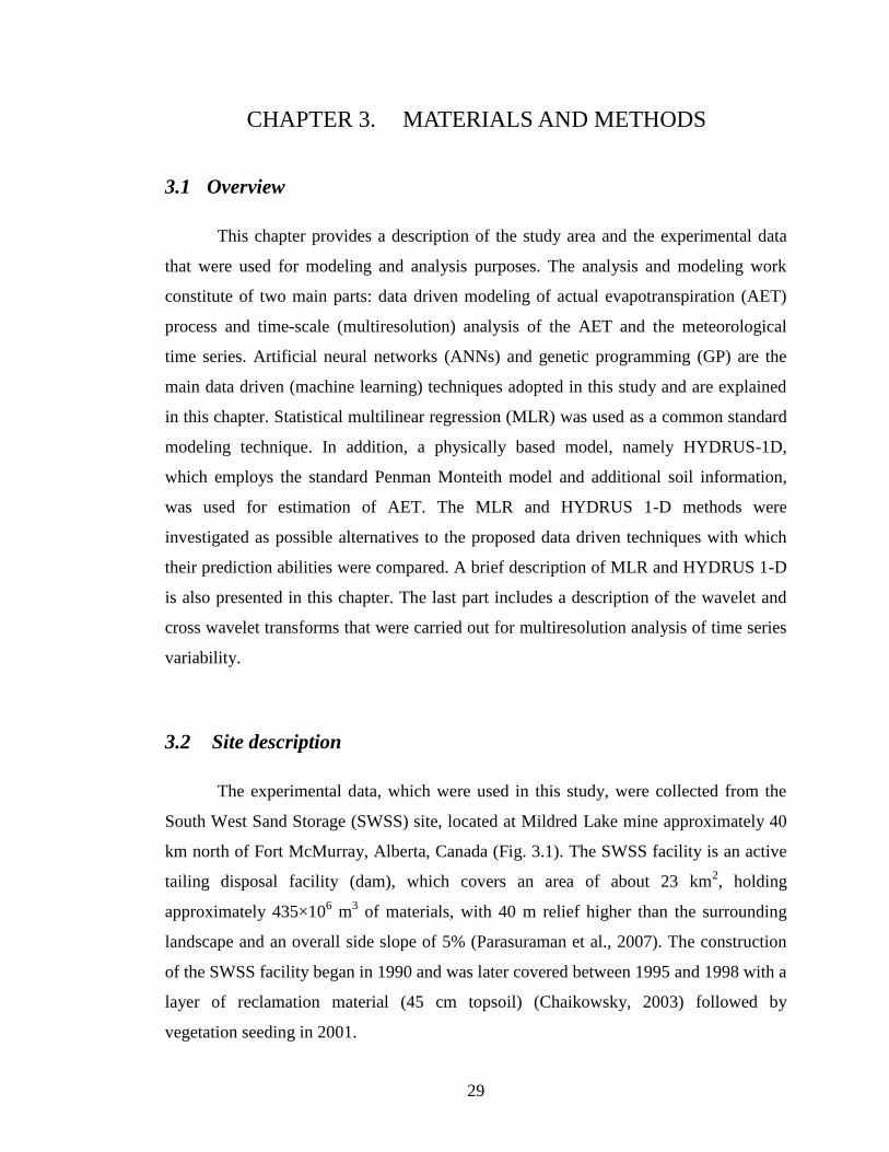
29

CHAPTER 3. MATERIALS AND METHODS

3.1 Overview

This chapter provides a description of the study area and the experimental data

that were used for modeling and analysis purposes. The analysis and modeling work

constitute of two main parts: data driven modeling of actual evapotranspiration (AET)

process and time-scale (multiresolution) analysis of the AET and the meteorological

time series. Artificial neural networks (ANNs) and genetic programming (GP) are the

main data driven (machine learning) techniques adopted in this study and are explained

in this chapter. Statistical multilinear regression (MLR) was used as a common standard

modeling technique. In addition, a physically based model, namely HYDRUS-1D,

which employs the standard Penman Monteith model and additional soil information,

was used for estimation of AET. The MLR and HYDRUS 1-D methods were

investigated as possible alternatives to the proposed data driven techniques with which

their prediction abilities were compared. A brief description of MLR and HYDRUS 1-D

is also presented in this chapter. The last part includes a description of the wavelet and

cross wavelet transforms that were carried out for multiresolution analysis of time series

variability.

3.2 Site description

The experimental data, which were used in this study, were collected from the

South West Sand Storage (SWSS) site, located at Mildred Lake mine approximately 40

km north of Fort McMurray, Alberta, Canada (Fig. 3.1). The SWSS facility is an active

tailing disposal facility (dam), which covers an area of about 23 km2, holding

approximately 435×106 m

3 of materials, with 40 m relief higher than the surrounding

landscape and an overall side slope of 5% (Parasuraman et al., 2007). The construction

of the SWSS facility began in 1990 and was later covered between 1995 and 1998 with a

layer of reclamation material (45 cm topsoil) (Chaikowsky, 2003) followed by

vegetation seeding in 2001.

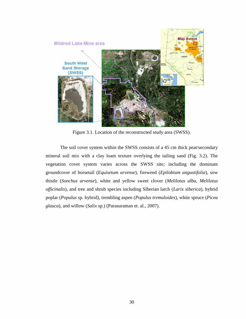
30

Figure 3.1. Location of the reconstructed study area (SWSS).

The soil cover system within the SWSS consists of a 45 cm thick peat/secondary

mineral soil mix with a clay loam texture overlying the tailing sand (Fig. 3.2). The

vegetation cover system varies across the SWSS site; including the dominant

groundcover of horsetail (Equisetum arvense), fireweed (Epilobium angustifolia), sow

thistle (Sonchus arvense), white and yellow sweet clover (Melilotus alba, Melilotus

officinalis), and tree and shrub species including Siberian larch (Larix siberica), hybrid

poplar (Populus sp. hybrid), trembling aspen (Populus tremuloides), white spruce (Picea

glauca), and willow (Salix sp.) (Parasuraman et. al., 2007).

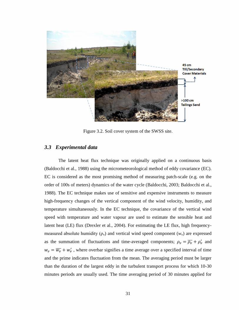
31

Figure 3.2. Soil cover system of the SWSS site.

3.3 Experimental data

The latent heat flux technique was originally applied on a continuous basis

(Baldocchi et al., 1988) using the micrometeorological method of eddy covariance (EC).

EC is considered as the most promising method of measuring patch-scale (e.g. on the

order of 100s of meters) dynamics of the water cycle (Baldocchi, 2003; Baldocchi et al.,

1988). The EC technique makes use of sensitive and expensive instruments to measure

high-frequency changes of the vertical component of the wind velocity, humidity, and

temperature simultaneously. In the EC technique, the covariance of the vertical wind

speed with temperature and water vapour are used to estimate the sensible heat and

latent heat (LE) flux (Drexler et al., 2004). For estimating the LE flux, high frequency-

measured absolute humidity (ρv) and vertical wind speed component (wv) are expressed

as the summation of fluctuations and time-averaged components; and

, where overbar signifies a time average over a specified interval of time

and the prime indicates fluctuation from the mean. The averaging period must be larger

than the duration of the largest eddy in the turbulent transport process for which 10-30

minutes periods are usually used. The time averaging period of 30 minutes applied for

32

the LE data were used in this study. The LE flux is then estimated as

, which

is equal to the mean covariance of the fluctuations of the vertical wind and absolute

humidity from their means (Drexler et al., 2004). λ is the latent heat of vaporization.

Using EC technique it is possible to do the calculations in real time as fast as the

readings are taken (Strangeways, 2003). ―The accuracy of the EC technique ranges from

±15% to ±20% of the actual evapotranspiration for hourly values‖ (Strangeways, 2003).

In addition to the high level precision and high degree of temporal and spatial resolution

of the EC technique in direct measurement of LE, it has an exceptional property of self-

verification, in case when other components of the energy balance closure can be

computed at the same time. Drexler et al. (2004) stated that no other methods have this

self-verification property.

The latent heat (LE) flux measurement system on the SWSS site consisted of a

triaxial sonic anemometer (CSAT3, Campbell Scientific, USA), for capturing the high-

frequency wind vector, an open-path infrared gas analyser (LI-7500, Li-Cor, USA) as a

humidity sensor and a fine-wire thermocouple, for recording the temperature

fluctuations, located in the approximate center of the sonic head about 2.9 m above the

ground surface. All measurements and their fluctuations were obtained at a frequency of

10 Hz and the mean fluxes were recorded every 30 minutes on a CR23X datalogger

(Campbell Scientific, USA) (Carey, 2008). The quantities are measured at high

frequency to record the most rapid fluctuations that are important to the process (Drexler

et al., 2004).

The EC tower was equipped with instrumentation to measure supplemental data

including long- and short-wave radiation (CNR1 net radiometer, Kipp and Zonen,

Netherlands) and wind speed (015A MetOne, USA) at 3.1 m above the ground, air

temperature and relative humidity (HMP45C, Vaisala Oyj, Finland) at 3 m, and ground

temperature (TCAV-L thermopile, Campbell Scientific, USA) at 0.03 m below the soil

surface. The supplemental data were sampled at 1 minute intervals and recorded every

half hour on a CR23X datalogger (Carey, 2008). Figure 3.3 shows the EC tower on the

SWSS site.

33

The LE and net radiation (Rn) fluxes were originally recorded in W.m-2

on a half

hourly basis. For convenient interpretation, the latent heat flux [W.m-2

] was converted to

the equivalent depth of water [mm.m-2

]. This was implemented using the following

equations (Dingman, 2002):

[3.1]

[3.2]

where, AET is the rate of actual evapotranspiration [mm/ 0.5hr], LE is the latent heat

energy [MJm-2

0.5hr-1

], T is the mean half-hour temperature [oC], λ is the latent heat of

vaporization [MJkg-1

] and ρw is the water density [kg.m

-3]. Air temperature (Ta;

oC),

ground temperature (Tg; oC), relative humidity (RH), and wind speed (Ws; m.s

-1)

constituted the rest of the meteorological data used for this study. Since the hourly time

scale of the data was the subject of study, conversion of the recorded half-hourly data to

hourly data was also implemented in the pre-processing step.

In data driven modeling, it is important to have large enough collection of data,

which contain several different instances for appropriately capturing the investigated

function. Using short time intervals, e.g. hourly, large number of instances can be used

for modeling, especially when the available measured data are associated with limited

time period. For instance, for the current case study, only two years of data are available

from which 1207 hourly instances can be obtained for modeling the ET process.

However, if daily time step is used, only 102 instances would be available.

Consequently, the hourly time scale of the data was selected for the current modeling

study. AET variations at small time-scales are also important because this type of

variation is more challenging than the larger scales and is important to be modeled and

analyzed. There are many water related functions (e.g. water quality) in engineering that

needs to be estimated at small-scales for which the rate of evapotranspiration at the same

time-scale is required. Small time-scale models can always be used for estimation of

larger-scale variations, by aggregating the small-scale predicted values. However, the

other way round might not be easily possible. For consistency in the data driven

w

LEAET

)(1000

)()10(36.25.2 3 T

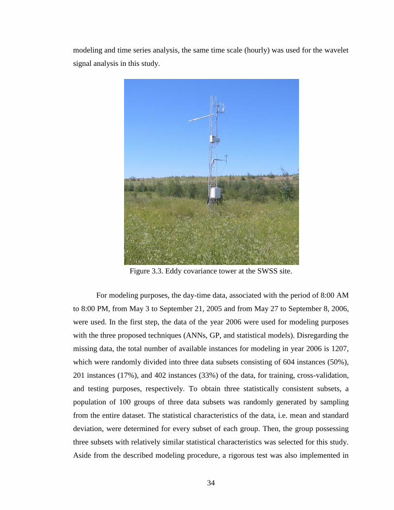
34

modeling and time series analysis, the same time scale (hourly) was used for the wavelet

signal analysis in this study.

Figure 3.3. Eddy covariance tower at the SWSS site.

For modeling purposes, the day-time data, associated with the period of 8:00 AM

to 8:00 PM, from May 3 to September 21, 2005 and from May 27 to September 8, 2006,

were used. In the first step, the data of the year 2006 were used for modeling purposes

with the three proposed techniques (ANNs, GP, and statistical models). Disregarding the

missing data, the total number of available instances for modeling in year 2006 is 1207,

which were randomly divided into three data subsets consisting of 604 instances (50%),

201 instances (17%), and 402 instances (33%) of the data, for training, cross-validation,

and testing purposes, respectively. To obtain three statistically consistent subsets, a

population of 100 groups of three data subsets was randomly generated by sampling

from the entire dataset. The statistical characteristics of the data, i.e. mean and standard

deviation, were determined for every subset of each group. Then, the group possessing

three subsets with relatively similar statistical characteristics was selected for this study.

Aside from the described modeling procedure, a rigorous test was also implemented in

35

the second step, using the data of 2005, to assess the generalization ability of the

developed models in a more realistic way. Disregarding the missing data in 2005, 1600

instances are available. The 2005 dataset has different statistical properties from the data

of 2006, which are discussed later in this study.

Multiresolution analysis of the AET and meteorological signals (wavelet

analysis) was conducted using the data of the year 2006. Since wavelet analysis (WA)

cannot be applied to a non-continuous time series, which contains a gap or missing data,

gap filling was performed to obtain a continuous time series. In the dataset of the year

2006, only AET time series contained missed values, which were filled using the most

fitted AET model developed in this study using the 2006 data (statistical multilinear

regression). The total number of instances that were available for wavelet analysis of the

2006 data is 2520, which constitute the hourly data from May 27 to September 9. All of

the observed time series data were pre-treated before performing the WA. The time

series data were standardized, following Grinsted et al. (2004), by subtracting the mean

value and then dividing by the standard deviation (zero mean and unit standard

deviation) for convenience when the results were compared.

The air temperature during the growing season of the year 2006 varied between 7

to 34 oC with an average value of 21

oC. The average day-time net radiation flux and

relative humidity were about 230.11 W/m2

and 0.51, respectively. The total rainfall

received during the growing season of 2006 was approximately 226.2 mm. During the

growing season of 2005, the air temperature ranged between -4 to 29 oC, with the

average of 17 oC. The average day-time net radiation flux and relative humidity values

were 215.36 W/m2 and 0.53, respectively. The total received rainfall during the growing

season of 2005 was 279.2 mm. The normal rainfall in the Fort McMurray is about 307.9

mm for the period of May to September. The average soil water content in the top 45 cm

of the soil during the studied periods of years 2005 and 2006 were 0.296 and 0.264

cm3/cm

3, respectively

36


3.4.1 Artificial Neural Networks (ANNs)

ANNs (Swingler, 1996) are massive networks of parallel information processing

systems resembling (simulating) the human brain’s analytical function, and they have an

inherent ability to learn and recognize highly nonlinear and complex relationships by

experience. ANNs learn from empirical examples, which make them a non-rule-based

technique, like statistical methods (Maier and Dandy, 2000). ANNs use mathematical

transfer functions to relate target variables to predictor (input) variables (Dawson and

Wilby, 2001).

Each neuron (information-processing unit) in ANNs consists of input connection

links, a central processing unit, and output connection links (Fig. 3.4). Input signals are

received through the connection links from the outside environment or other neurons.

Each connection link is assigned a synaptic weight (w) representing the strength of the

connection between two nodes in characterizing input-output relationship (ASCE,

2000a). Received information is processed in the central processing unit (neuron body),

by adding up the weighted inputs and bias (Eq. 3.3), and passed through the activation

function (Eq. 3.4). Bias (b) is the threshold value, which must be exceeded before the

node (neuron) can be activated (ASCE, 2000a). Activation function forms the output of

the node and enables the nonlinear transformation of inputs to outputs. The type of

activation function, which can be sigmoid, linear, threshold, Gaussian, or hyperbolic

tangent function (Dawson and Wilby, 2001), depends on the network’s type and

associated training algorithm. The log-sigmoid activation function is one of the two most

commonly used activation functions in the literature because it is continuous, relatively

easy to compute, its derivatives are simple (during the training process), maps the

outputs away from extremes, and provide nonlinear response (ASCE, 2000a).

[3.3]

[3.4]

bxwt i

n

i

i 1

tetf

1

1)(

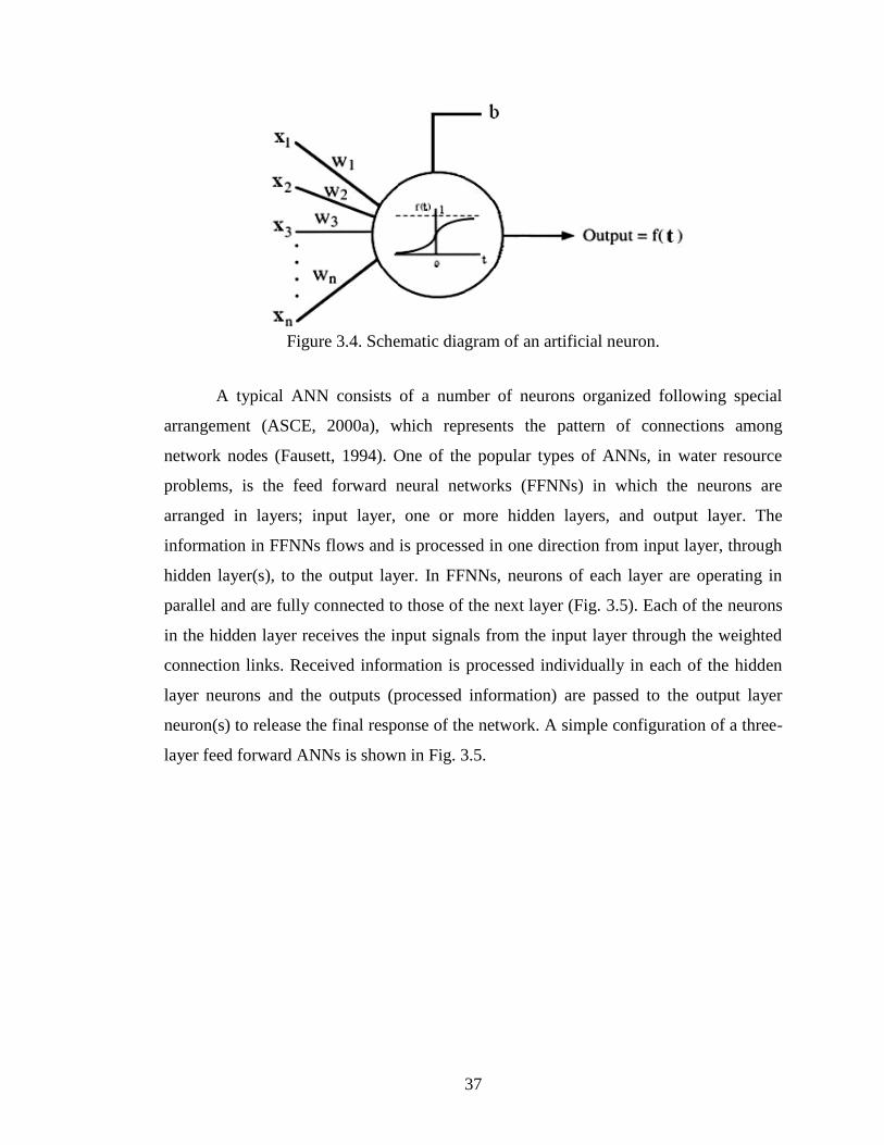
37

Figure 3.4. Schematic diagram of an artificial neuron.

A typical ANN consists of a number of neurons organized following special

arrangement (ASCE, 2000a), which represents the pattern of connections among

network nodes (Fausett, 1994). One of the popular types of ANNs, in water resource

problems, is the feed forward neural networks (FFNNs) in which the neurons are

arranged in layers; input layer, one or more hidden layers, and output layer. The

information in FFNNs flows and is processed in one direction from input layer, through

hidden layer(s), to the output layer. In FFNNs, neurons of each layer are operating in

parallel and are fully connected to those of the next layer (Fig. 3.5). Each of the neurons

in the hidden layer receives the input signals from the input layer through the weighted

connection links. Received information is processed individually in each of the hidden

layer neurons and the outputs (processed information) are passed to the output layer

neuron(s) to release the final response of the network. A simple configuration of a three-

layer feed forward ANNs is shown in Fig. 3.5.

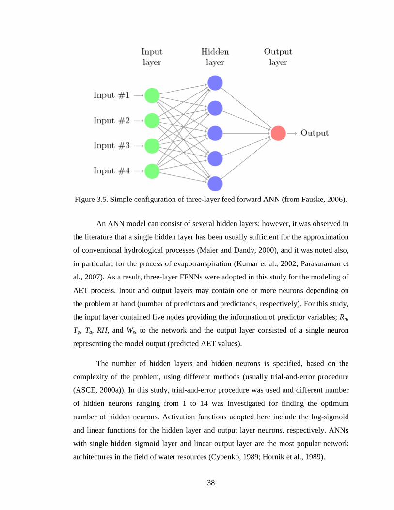
38

Figure 3.5. Simple configuration of three-layer feed forward ANN (from Fauske, 2006).

An ANN model can consist of several hidden layers; however, it was observed in

the literature that a single hidden layer has been usually sufficient for the approximation

of conventional hydrological processes (Maier and Dandy, 2000), and it was noted also,

in particular, for the process of evapotranspiration (Kumar et al., 2002; Parasuraman et

al., 2007). As a result, three-layer FFNNs were adopted in this study for the modeling of

AET process. Input and output layers may contain one or more neurons depending on

the problem at hand (number of predictors and predictands, respectively). For this study,

the input layer contained five nodes providing the information of predictor variables; Rn,

Tg, Ta, RH, and Ws, to the network and the output layer consisted of a single neuron

representing the model output (predicted AET values).

The number of hidden layers and hidden neurons is specified, based on the

complexity of the problem, using different methods (usually trial-and-error procedure

(ASCE, 2000a)). In this study, trial-and-error procedure was used and different number

of hidden neurons ranging from 1 to 14 was investigated for finding the optimum

number of hidden neurons. Activation functions adopted here include the log-sigmoid

and linear functions for the hidden layer and output layer neurons, respectively. ANNs

with single hidden sigmoid layer and linear output layer are the most popular network

architectures in the field of water resources (Cybenko, 1989; Hornik et al., 1989).

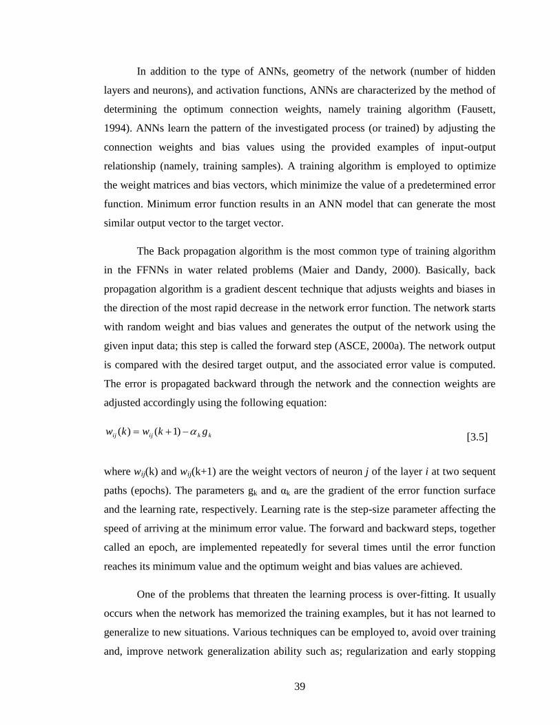
39

In addition to the type of ANNs, geometry of the network (number of hidden

layers and neurons), and activation functions, ANNs are characterized by the method of

determining the optimum connection weights, namely training algorithm (Fausett,

1994). ANNs learn the pattern of the investigated process (or trained) by adjusting the

connection weights and bias values using the provided examples of input-output

relationship (namely, training samples). A training algorithm is employed to optimize

the weight matrices and bias vectors, which minimize the value of a predetermined error

function. Minimum error function results in an ANN model that can generate the most

similar output vector to the target vector.

The Back propagation algorithm is the most common type of training algorithm

in the FFNNs in water related problems (Maier and Dandy, 2000). Basically, back

propagation algorithm is a gradient descent technique that adjusts weights and biases in

the direction of the most rapid decrease in the network error function. The network starts

with random weight and bias values and generates the output of the network using the

given input data; this step is called the forward step (ASCE, 2000a). The network output

is compared with the desired target output, and the associated error value is computed.

The error is propagated backward through the network and the connection weights are

adjusted accordingly using the following equation:

[3.5]

where wij(k) and wij(k+1) are the weight vectors of neuron j of the layer i at two sequent

paths (epochs). The parameters gk and αk are the gradient of the error function surface

and the learning rate, respectively. Learning rate is the step-size parameter affecting the

speed of arriving at the minimum error value. The forward and backward steps, together

called an epoch, are implemented repeatedly for several times until the error function

reaches its minimum value and the optimum weight and bias values are achieved.

One of the problems that threaten the learning process is over-fitting. It usually

occurs when the network has memorized the training examples, but it has not learned to

generalize to new situations. Various techniques can be employed to, avoid over training

and, improve network generalization ability such as; regularization and early stopping

kkijij gkwkw )1()(

40

(Neural Network Toolbox User’s Guide, 2009). Regularization attempts to smooth the

network response by keeping the size of the network weights adequately small

(MacKay, 1992) using the modified form of the error function, which considers network

weights and biases (Neural Network Toolbox User’s Guide, 2009). Benefiting from the

regularization method, the modified error function (msereg) that was employed in the

training process of ANNs in this study is given as:

[3.6]

where Oi, Pi, N, γ, and wj are the target output, ANN predicted output, number of

training samples, performance ratio, and network weights, respectively.

Through the early stopping approach, an independent test set, namely cross-

validation, can be used to monitor the performance of the model on a set of not-yet-

encountered examples at some stages of the training process. Training is stopped when

error on the cross-validation dataset begins to rise to prevent the model from being over-

trained (Neural Network Toolbox User’s Guide, 2009). In this study, both regularization

and early stopping approaches were employed with the examined training algorithms;

Levenberg-Marquardt (Levenberg, 1944; Marquardt, 1963) and Bayesian-regularization

(MacKay, 1992). Levenberg-Marquardt is one of the high-performance algorithms that

appear to be the fastest method for training moderate-sized FFNNs (Neural Network

Toolbox User’s Guide, 2009). Bayesian-regularization algorithm is an automated

regularization algorithm, which uses Bayesian framework to automatically determine the

optimal regularization parameter, performance ratio (γ), in the modified performance

function. This algorithm also provides a measure of network parameters (weight and

biases) that are being effectively used by the network. This ensures that the network will

not use a larger number of parameters than the identified effective ones in estimating

network output values. In other words, it keeps the network size as small as possible

(Neural Network Toolbox User’s Guide, 2009).

Neural Network Toolbox in MATLAB (MATLAB® Software, 2003) was used

to develop the ANN models to predict AET based on five inputs of meteorological

m

j

ji

N

i

i wN

PON

msereg1

22

1

)1()(

41

variables, Rn, Tg, Ta, Ws, and RH. The data pool of 2006 was randomly divided into three

subsets of training, cross validation, and testing using the approach explained earlier.

The employed approach for splitting the data pool ensured that all three sub datasets

were fairly representing the population to be modeled. The training subset was used for

optimizing the connection weight matrices and bias vectors of the network. The cross-

validation subset was used to stop the training process when the network starts to over-

fit the training subset (early stopping). Once the network was trained, the generalization

and predictive ability of the network was evaluated using a completely unseen subset of

2006 called testing subset.

The data subsets were normalized so that data fell between 0 and 1. Such scaling

of data smoothes the solution space and averages out some of the noise effects (ASCE,

2000a). Based on the training subset, different ANN models were trained using

Levenberg-Marquardt and Bayesian-regularization training algorithms, using different

number of hidden neurons ranging from 1 to 14. For each examined network

architecture, the training process was repeated several times, each time started with

different random initial weight matrices, until satisfactory optimal network (with

minimum errors) was obtained. The ANN model with the best performance measures

associated with the cross-validation subset was selected as the optimal predictive

network. The performance and generalization ability of the trained model was evaluated

on the testing subset. This model validation determines how well the ANN model

performs on the dataset that have not been seen during the training process (Cheng and

Titterington, 1994).

ANNs, as a data driven technique, have the ability to determine the critical model

inputs (Maier and Dandy, 2000). In this study, the ANN modeling technique was used to

identify the important meteorological variables affecting the AET process. In this

approach, no prior knowledge was assumed about the physics of AET mechanism and

the relationships among variables. All possible combinations of input variables, 26

combinations, were considered to be examined as ANN model input sets. Separate

optimal ANN models were developed and trained for each input combination set using

the model development approach explained earlier. The developed ANN models were

42

compared based on their prediction accuracy in order to identify the most appropriate

and efficient combinations of inputs for the estimation of AET. This approach is

commonly referred to as trial-and-error procedure, which is under the category of

heuristic approaches. The possible combination sets of five available input variables

include; five-input combination, ―Rn, Tg, Ta, RH, Ws‖, four-input combinations, ―Rn, Tg,

RH, Ws‖; ―Rn, Tg, Ta, RH‖; ―Rn, Tg, Ta, Ws‖; ―Rn, Ta, RH, Ws‖; ―Tg, Ta, RH, Ws‖; three-

input combinations, ―Rn, Tg, RH‖; ―Rn, Tg, Ws‖; ―Rn, Tg, Ta‖; ―Rn, RH, Ws‖; ―Rn, Ta, RH‖;

―Rn, Ta, Ws‖; ―Tg, RH, Ws‖; ―Tg, Ta, Ws‖; ―Tg, Ta, RH‖; ―Ta, RH, Ws‖; and two-input

combinations, ―Rn, Tg‖ ; ―Rn, RH‖ ; ―Rn, Ws‖ ―Rn, Ta‖ ; ―Tg, RH‖ ; ―Tg, Ws‖ ; ―Tg, Ta‖ ;

―Ta, RH‖ ; ―Ta, Ws‖ ; ―RH, Ws‖.

3.4.2 Genetic programming (GP)

Genetic algorithms (GA) belong to the family of evolutionary algorithms, and

are generally considered as an optimization method for searching global optimum of a

function using natural genetic operators. Genetic programming (GP), which was

introduced by Koza (1992), is an extension of GA for inducing computer programs, as

solutions for problems at hand, using an intelligent and adaptive search. This type of

search uses the information gained from the performance (fitness) of individual

computer programs, in the search space, for modifying and improving the current

programs. Depending on the particular problem, computer programs of the GP search

space may be different, e.g. Boolean-valued models and symbolic mathematical models

(Koza, 1992). Symbolic regression GP evolves computer programs in the form of

mathematical expressions in which both functional form and numerical coefficients of

the regression symbolic model are optimized through the evolutionary process of GP.

This application of GP was adopted in this study for obtaining explicit mathematical

AET models.

In the first step of GP implementation, a population of computer programs are

randomly generated using no primary knowledge about the optimum solution (e.g.

structure of the underlying relationship model) and possible relationships among

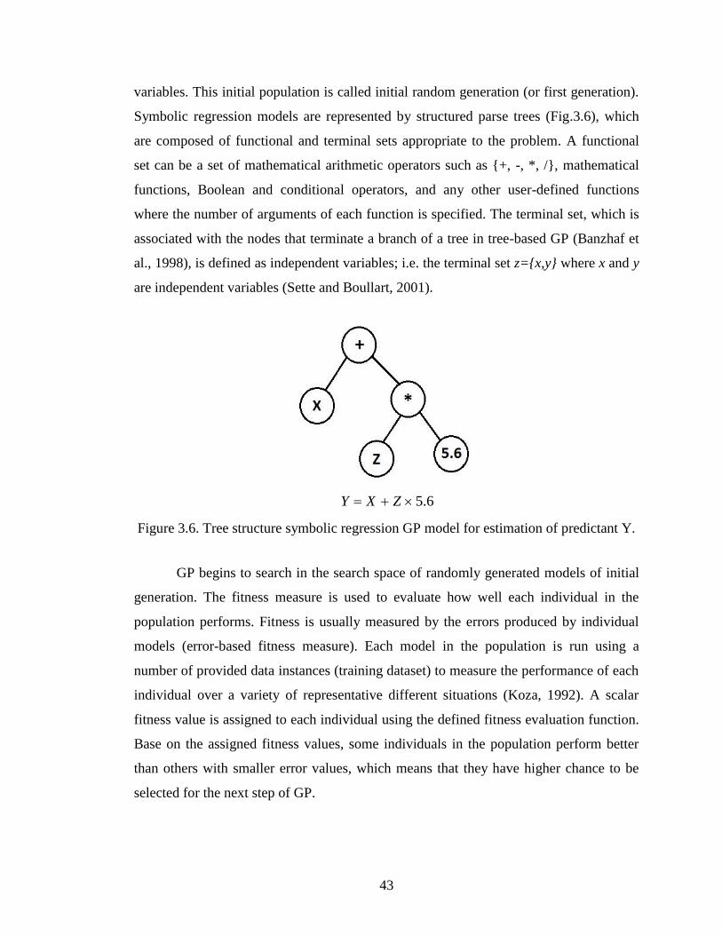
43

variables. This initial population is called initial random generation (or first generation).

Symbolic regression models are represented by structured parse trees (Fig.3.6), which

are composed of functional and terminal sets appropriate to the problem. A functional

set can be a set of mathematical arithmetic operators such as {+, -, *, /}, mathematical

functions, Boolean and conditional operators, and any other user-defined functions

where the number of arguments of each function is specified. The terminal set, which is

associated with the nodes that terminate a branch of a tree in tree-based GP (Banzhaf et

al., 1998), is defined as independent variables; i.e. the terminal set z={x,y} where x and y

are independent variables (Sette and Boullart, 2001).

Figure 3.6. Tree structure symbolic regression GP model for estimation of predictant Y.

GP begins to search in the search space of randomly generated models of initial

generation. The fitness measure is used to evaluate how well each individual in the

population performs. Fitness is usually measured by the errors produced by individual

models (error-based fitness measure). Each model in the population is run using a

number of provided data instances (training dataset) to measure the performance of each

individual over a variety of representative different situations (Koza, 1992). A scalar

fitness value is assigned to each individual using the defined fitness evaluation function.

Base on the assigned fitness values, some individuals in the population perform better

than others with smaller error values, which means that they have higher chance to be

selected for the next step of GP.

6.5 ZXY

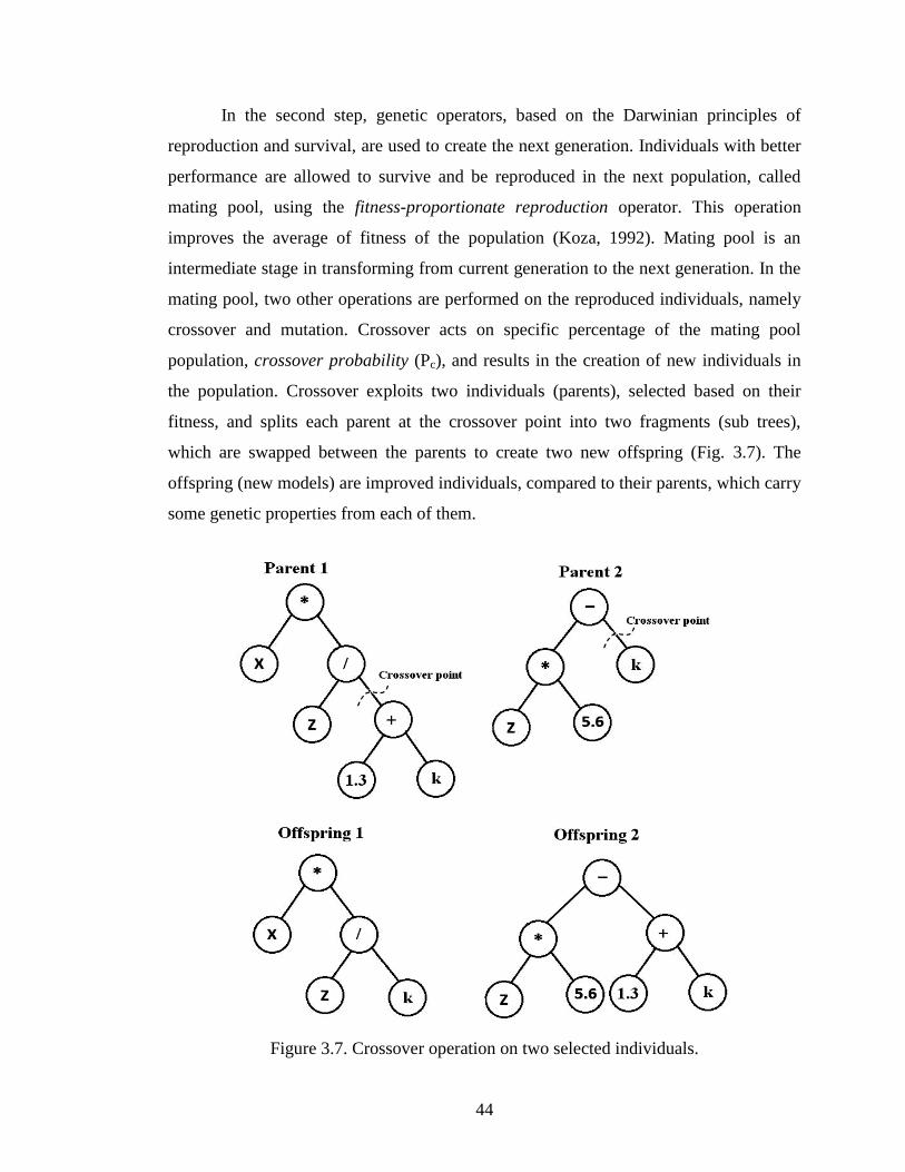
44

In the second step, genetic operators, based on the Darwinian principles of

reproduction and survival, are used to create the next generation. Individuals with better

performance are allowed to survive and be reproduced in the next population, called

mating pool, using the fitness-proportionate reproduction operator. This operation

improves the average of fitness of the population (Koza, 1992). Mating pool is an

intermediate stage in transforming from current generation to the next generation. In the

mating pool, two other operations are performed on the reproduced individuals, namely

crossover and mutation. Crossover acts on specific percentage of the mating pool

population, crossover probability (Pc), and results in the creation of new individuals in

the population. Crossover exploits two individuals (parents), selected based on their

fitness, and splits each parent at the crossover point into two fragments (sub trees),

which are swapped between the parents to create two new offspring (Fig. 3.7). The

offspring (new models) are improved individuals, compared to their parents, which carry

some genetic properties from each of them.

Figure 3.7. Crossover operation on two selected individuals.

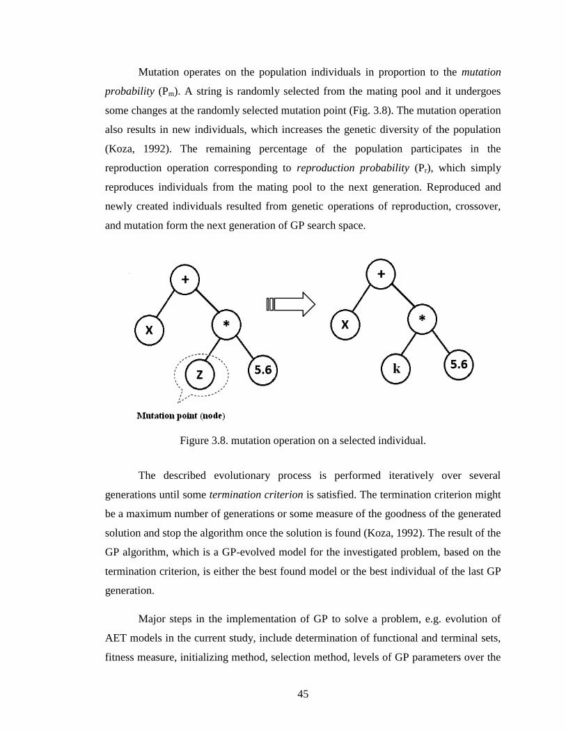
45

Mutation operates on the population individuals in proportion to the mutation

probability (Pm). A string is randomly selected from the mating pool and it undergoes

some changes at the randomly selected mutation point (Fig. 3.8). The mutation operation

also results in new individuals, which increases the genetic diversity of the population

(Koza, 1992). The remaining percentage of the population participates in the

reproduction operation corresponding to reproduction probability (Pr), which simply

reproduces individuals from the mating pool to the next generation. Reproduced and

newly created individuals resulted from genetic operations of reproduction, crossover,

and mutation form the next generation of GP search space.

Figure 3.8. mutation operation on a selected individual.

The described evolutionary process is performed iteratively over several

generations until some termination criterion is satisfied. The termination criterion might

be a maximum number of generations or some measure of the goodness of the generated

solution and stop the algorithm once the solution is found (Koza, 1992). The result of the

GP algorithm, which is a GP-evolved model for the investigated problem, based on the

termination criterion, is either the best found model or the best individual of the last GP

generation.

Major steps in the implementation of GP to solve a problem, e.g. evolution of

AET models in the current study, include determination of functional and terminal sets,

fitness measure, initializing method, selection method, levels of GP parameters over the

46

run (crossover and mutation probabilities, population size), and the termination criterion.

The functional set, which was introduced to GP, included {+, -,*, /}. The terminal set

was defined as {Rn, Tg, Ta, Ws, RH}. Root mean squared error (RMSE) was selected as

the fitness function for evaluating individual performance and further fitness-based

selection. Ramped-half-and-half method was adopted for initializing the first generation

tree structures. This initializing method increases the diversity of the tree structures

using various shapes and sizes by mixing two common methods of tree initializing,

namely, full method and grow method. Further descriptions of initializing methods can

be found in Koza (1992) and Banzhaf et al. (1998).

The next important issue in the implementation of GP is the fitness-based

selection method. Selection method determines the manner by which the individuals are

selected based on the assigned fitness values for further GP operations (e.g. crossover,

mutation). Roulette wheel selection method was employed for implementing selection

operation in the GP runs. Roulette wheel method is the simplest selection scheme that

follows a stochastic algorithm. In this method, individuals are attached to contiguous

slices of a roulette wheel; each slice is proportional in size to the fitness value of the

attached individual. A random number is generated and the individual whose slice spans

the random number is selected. Following this method, individuals with better fitness

values were given larger chance to be selected and passed into the next generation.

Several different levels of GP parameters; crossover and mutation probabilities, number

of evaluated generations, and the size of population, were executed for obtaining

symbolic regression AET models using the training subset. The termination criterion for

each GP run was the identified maximum number of generations. The performances of

the generated symbolic equations were assessed using the cross-validation subset to

select the best equation (model). The selected symbolic equation was then tested using

the unseen testing subset to evaluate the predictive accuracy and generalization ability of

the proposed model.

Data subsets that were used with the GP technique were exactly the same as

those used with the ANNs. The data were normalized by dividing the values of variables

by their corresponding maximum values. In this way, all variables could have

47

dimensional consistency during the GP implementation (Parasuraman et al., 2007). In

this study, GPLAB (Silva, 2005), GP toolbox for MATLAB, was used for the

implementing of the GP technique and generating mathematical models based on the

datasets where AET is a dependent variable as a function of the five independent

variables: Rn, Tg, Ta, Ws, and RH.

3.4.3 Multilinear regression (MLR)

Linear regression is a conventional approach in the statistical modeling of the

relationship between variables in which the unknown parameters of the regression model

are estimated using the data instances. Multilinear regression (MLR) is a statistical

model that contains more than one predictor variable. The general form of the first order

MLR model is:

[3.7]

where Y is the dependent variable (predictant) that is represented as a function of n

independent variables (predictors), X. β0 is the unknown intercept, β1, ... , βn are the

unknown coefficients (also called partial regression coefficients) of the function, and ε is

the random error term with assumed normal distribution.

Since the statistical regression is the simplest and most straight forward form of a

model, it is usually the first modeling approach that is adopted and investigated for

modeling of a relationship (Laverty, 2009) and might be considered as a benchmark

modeling approach. Many nonlinear models can be represented in the form of linear

models by appropriately transforming any or all of the independent variables. In this

way, nonlinear models are linearized and the unknown parameters are estimated

(specified) using the simple method of linear regression. Equation (3.7) is the standard

form of the MLR, which includes only the first order of the independent variables. Two

other forms of the MLR, which were employed for the statistical modeling of AET

process in this study, are given below:

nn XXXY ...22110

48

[3.8]

[3.9]

Equation (3.8) includes the linear terms and the cross-product terms of the two predictor

variables, which are referred to as interaction effect. Interaction refers to the effect that a

change in a predictor variable can have on the predictand depends on the level of the

other predictor variable(s) (ReliaSof’s DOE++ software User’s Guide, 2008). In Eq.

(3.9), in addition to the already defined terms of linear and interaction, the higher order

terms (second order here) of the predictor variables are considered. Both given

regression functions, Eq. (3.8) and (3.9), are still linear because the models are linear in

parameters (ReliaSof’s DOE++ software User’s Guide, 2008). Consequently, they can

be expressed in the general form of Eq. (3.7), using the appropriate transformations such

as x1=X1.X2 and x2=X12, and then the unknown parameters are specified using the data

samples. This approach was used in this study for fitting the statistical regression models

for the estimation of AET.

The experimental data of AET including the first and second orders of five

independent variables and all their two-factor interactions were statistically analyzed

using a statistical analysis software (SAS/STAT® software, 2003). All data subsets

employed in the statistical analysis were exactly the same as those used with ANNs and

GP techniques. Using the training subset, two different MLR equations were developed

by following the functional forms of the Eq. (3.8) and (3.9). In addition, as a baseline

comparison, a simple first order regression equation (Eq. 3.7) was fitted to the data using

the linear factors of the meteorological variables; Rn, Tg, Ta, Ws, and RH. The best

equation was selected based on the error statistics associated with the cross-validation

dataset.

In the first developed statistical model, the input variables introduced to the

SAS/STAT® software included the linear factors of the meteorological variables, Rn, Tg,

Ta, Ws, and RH, and all of their two-factor interactions, TaTg, TaRH, TaRn, TaWs, TgRH,

131221122110 ...... nnknnnnn XXXXXXXXXY

22

11

1312211110

...

......

nmkn

nnknnnnn

XX

XXXXXXXXY

49

TgRn, TgWs, RHRn, RHWs, and RnWs. For the second statistical model, in addition to the

already defined input variables, the second orders of the meteorological variables, Rn2,

Tg2, Ta

2, Ws

2 and RH

2, were also considered. The stepwise selection method was

performed to fit the multilinear regression equations and to assess the significance of the

introduced variables on the AET process. The stepwise method uses both forward and

backward selection techniques for finding the best model that is also adequately simple

(containing all important variables). The least squares method was employed for

identifying the unknown parameters of the MLR models. In this method, the regression

parameters of β0, β1, β2,…, βm are estimated to minimize the residual sum of squares

(RSS) (Eq. 3.10) between observed and predicted values provided by the model over

fitness cases (training subset). RSS fitness function is defined as:

RSS= [3.10]

where Yi, Yi´, and N are observed value, predicted value, and number of training

samples, respectively. To identify the terms having significant effects on AET, the tests

of hypothesis was conducted at 95% confidence level.

3.5 HYDRUS-1D model

The main idea behind the use of the HYDRUS model was to compare a currently

available AET estimation model with the proposed data driven models. The predictive

abilities of some data driven models, e.g. ANNs and GP, have already been compared

with that of the widely used standard FAO Penman-Monteith (PM) method

(Parasuraman, et al., 2007). However, the standard PM method estimates the potential

evapotranspiration, since it assumes that the soil moisture is not a limiting factor.

Therefore, this comparison with the data driven AET models may not seem appropriate.

In order to perform such comparison more reasonably, one of the available methods for

estimation of AET was employed, through using HYDRUS-1D software modeling

package (Version 4.0; Šimunek et al., 2006), and its performance was compared with

those of the developed data driven models.

2

1

)'( i

N

i

i YY

50

One of the most widely used methods for the estimation of AET is to make use

of meteorological data and the commonly available reference evapotranspiration (ETo)

models and compute the AET using the soil wetness function (f(θrel)), Eq. (3.11),

(Dingman, 2002). Soil wetness function describes the relationship between AET/ETo

and relative water content, θrel.

[3.11]

where is defined as:

[3.12]

where θ, θpwp, and θfc are the current water content, permanent wilting point, and field-

capacity of the soil. HYDRUS-1D is a physically based software package simulating the

water, heat, and solute movement in one-dimensional variably-saturated media.

HYDRUS-1D model can simulate the rate of actual evapotranspiration based on the

described method incorporated with some numerical methods. In this model, ETo is

estimated with the FAO recommended PM equation (Monteith, 1981; Monteith and

Unsworth, 1990; FAO, 1990), which is the widely adopted physically based model for

the modeling of ET. Then, the rate of AET is estimated using the PM-predicted ETo,

simulated soil moisture profile, and evaporation rate, which is described below.

For this type of AET modeling, in addition to the meteorological data of Rn, Ta,

RH, and Ws, the data of leaf area index (LAI) and rainfall were also required. The data of

LAI were available on an approximately weekly basis, which were disaggregated to

hourly basis using linear interpolation for consistency with temporal resolution of other

meteorological data. Rainfall data were also available in event-based records for which

some aggregation procedure was performed to obtain hourly rainfall data. Hydraulic

conductivities of the soil layers were optimized through an inverse simulation procedure

in HYDRUS-1D model. Other required physical and hydraulic parameters of the soil

were selected based on the previously conducted research on the same soil type

oET).( relfAET

rel

pwpfc

pwp

rel

51

(Shurniak, 2003). Using HYDRUS-1D software, ETo was determined with the FAO

recommended PM combination equation (FAO, 1990):

[3.13]

where ETo is the rate of potential evapotranspiration from reference crop [mm h-1

], λ is

the latent heat of vaporization [MJ kg-1

], Rn is net radiation at surface [MJ m-2

h-1

], G is

the soil heat flux [MJ m-2

h-1

], ρ is the air density [kg m-3

], cp is the specific heat of soil

moisture [kJ kg-1

oC

-1], (es-ea) is the vapour pressure deficit [kPa], es is the saturation

vapour pressure at temperature T [kPa], ea is the actual vapour pressure [kPa], rc is the

crop canopy resistance [s m-1

], ra is the aerodynamic resistance [s m-1

], γ' is the

psychrometric constant [kPa oC

-1], and Δ is the slope of the vapour pressure curve [kPa

oC

-1] (HYDRUS-1D Software Package User’s Manual, 2008).

Estimated ETo was partitioned into potential soil evaporation and potential plant

transpiration using the LAI information. Actual transpiration was then calculated from

the obtained potential transpiration and the plant water stress function proposed by Van

Genuchten (1978). The gradient of simulated water pressure head in the soil profile

along with the soil hydraulic conductivity were used for the simulation of actual

evaporation rate from the soil surface. Simulated evaporation was compared with the

calculated potential evaporation to give the actual rate of soil evaporation. This

comparison is performed because the PM model sometimes overestimates the rate of

evaporation. If the PM-estimated evaporation is larger than the simulated evaporation,

the simulated value is given as the actual rate of evaporation. Estimated values of actual

evaporation and transpiration were aggregated to estimate the actual rate of

evapotranspiration (AET). Because the HYDRUS model was not within the main scope

of this thesis, the detailed methodology associated with this type of modeling is not

provided here. Detailed description of AET simulation using HYDRUS-1D can be found

in HYDRUS-1D Software Package User’s Manual (2008). HYDRUS model was used

for estimation of AET in years 2005 and 2006 out of which the model comparison was

performed only based on the 2005 dataset. The reason for using 2005 data was that the

data driven models were trained using a large portion of 2006 data on which they

52

expectedly perform well. As a result, a fair model comparison can be performed using

the dataset of the year 2005.

3.6 Evaluation of models’ Performance

The performances of the data driven models; ANNs, GP, and multilinear

regression models, as well as the HYDRUS-1D model were evaluated to compare their

predictive accuracies based on three statistical criteria: Pearson’s correlation coefficient

(R), root mean squared error (RMSE), and mean absolute relative error (MARE), which

were calculated as follows:

[3.14]

[3.15]

[3.16]

where Oi, Pi, , and are observed values, simulated values, mean of simulated, and

mean of observed values, respectively. N is the number of instances in the dataset. In

addition to the above mentioned statistics, akaike’s information criterion (AIC) was used

for characterizing and comparing the goodness of fit of the obtained data driven models.

The AIC provides a measure of model quality, which rewards a model for goodness of

fit, but also penalizes it for unnecessary parameters. AIC is widely used for model

selection and is defined as (Akaike, 1974; Russo et al., 1991):

[3.17]

5.0

1

25.0

1

2

1

N

i

i

N

i

i

i

N

i

i

PPOO

PPOO

R

N

i i

ii

O

PO

NMARE

1

1

N

PO

RMSE

N

i

ii

1

2

P O

53

where SSE, k, and l are summation of squared error, number of observations and number

of parameters to be optimized during modeling. Smaller AIC value indicates more

approprite model.

3.7 Wavelet Analysis

Natural functions, e.g. meteorological and hydrological processes, operate over a

wide range of spatial and temporal scales leading to spatial/temporal variability of

interacting mechanisms. AET is a hydrometeorological signal (variable) interacting with

several temporally/spatially variable meteorological signals. Evaluation of dominant

cyclic variations in the AET and correlated meteorological signals improves the

understanding of the mechanism as well as its modeling. In this study, only temporal

scaling of the variables time series was investigated whereas the spatial variability of the

AET and meteorological signals was not considered.

Temporal cyclic variations of natural processes are not usually stationary and

contain several localized and transient frequency events. Therefore, conventional

frequency domain analysis such as Fourier transform can not reveal the localized natural

cyclic events, because in this kind of transformations the temporal variations of the

signal is separated at different scales only (Si, 2008). Wavelet analysis (WA) provides a

tool for decomposing the variations of a time series signal into time and scale

(frequency) domains; allowing the identification and analysis of dominant temporal

cyclic events. Theoretical description and a complete introduction of WA can be found

in Daubechies (1992) and Lau and Weng (1995). Torrence and Compo (1998) developed

an easy-to-use wavelet analysis toolkit, which includes statistical significance testing for

improving the qualitative nature of the WA. The same approach as Torrence and Compo

(1998) was employed in this study for WA of AET and meteorological time series.

The basic component of WA is the wavelet transformation in which the studied

function is represented by wave-like oscillating functions. The choice of the wavelet

function is of high importance within the wavelet transformation. Wavelet function is a

small finite-length oscillating mathematical function (small wave) (Polikar, 1996),

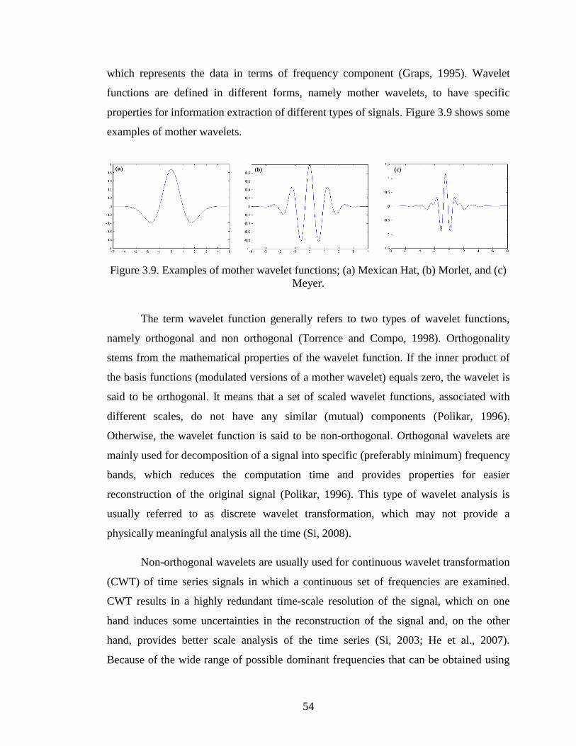
54

which represents the data in terms of frequency component (Graps, 1995). Wavelet

functions are defined in different forms, namely mother wavelets, to have specific

properties for information extraction of different types of signals. Figure 3.9 shows some

examples of mother wavelets.

Figure 3.9. Examples of mother wavelet functions; (a) Mexican Hat, (b) Morlet, and (c)

Meyer.

The term wavelet function generally refers to two types of wavelet functions,

namely orthogonal and non orthogonal (Torrence and Compo, 1998). Orthogonality

stems from the mathematical properties of the wavelet function. If the inner product of

the basis functions (modulated versions of a mother wavelet) equals zero, the wavelet is

said to be orthogonal. It means that a set of scaled wavelet functions, associated with

different scales, do not have any similar (mutual) components (Polikar, 1996).

Otherwise, the wavelet function is said to be non-orthogonal. Orthogonal wavelets are

mainly used for decomposition of a signal into specific (preferably minimum) frequency

bands, which reduces the computation time and provides properties for easier

reconstruction of the original signal (Polikar, 1996). This type of wavelet analysis is

usually referred to as discrete wavelet transformation, which may not provide a

physically meaningful analysis all the time (Si, 2008).

Non-orthogonal wavelets are usually used for continuous wavelet transformation

(CWT) of time series signals in which a continuous set of frequencies are examined.

CWT results in a highly redundant time-scale resolution of the signal, which on one

hand induces some uncertainties in the reconstruction of the signal and, on the other

hand, provides better scale analysis of the time series (Si, 2003; He et al., 2007).

Because of the wide range of possible dominant frequencies that can be obtained using

55

CWT, Coulibaly and Burn (2004) indicated that the CWT is more appropriate for

analysis of geophysical and hydrological time series. For the current study, scale

analysis of the time series data were of interest, so the CWT was employed and is

described here.

3.7.1 Continuous wavelet analysis

As it was mentioned earlier, the choice of wavelet function is an important

component in the wavelet transformation. Wavelet function can be a real or complex

function. Complex wavelet functions make it possible to extract the information of both

amplitude and phase, which is more suitable for analyzing the signal’s oscillatory

behaviour (Torrence and Compo, 1998). Morlet, Mexican Hat, and Haar are some of the

mother wavelets usually employed in the CWT out of which the Morlet is a complex

function. Depending on specific information one might be interested in, different

wavelet functions can be selected. The selected mother wavelet must satisfy some non-

restrict requirements, which assure the success of reconstruction procedure. This

mathematical condition is called the ―admissibility condition‖ at which the wavelet

function should have zero mean and quickly decay in both time and scale space (Farge,

1992). The latter condition represents the localization quality of the function in time and

space scale.

Morlet is a complex and non-orthogonal wavelet that provides sufficient

resolution (localization) in time and scale domains (Grinsted et al., 2004; Si, 2008).

Morlet function, with non-dimensional frequency parameter (ω0) equal to 6, has been

shown to successfully work for the analysis of observed time series in different

hydrological applications (Lafreniere and Sharp, 2003; Anctil and Tape, 2004; Coulibaly

and Burn, 2004; Labat et al., 2005; Si and Zelek, 2005; Coulibaly, 2006). This Morlet

wavelet was used for the current wavelet transformation, which is an exponential

oscillatory function defined as (Torrence and Compo, 1998):

[3.18] 2/4/1 2

)( ee oi

o

56

where η and ω0 are non-dimensional time and frequency parameters. The Morlet

wavelet with ω0 = 6 was adopted to satisfy the admissibility condition (Farge, 1992).

The CWT of a discrete time series data of xi (i=1,2,…,N) is defined as the inner

product (convolution) of time series signal with the scaled and translated version of

mother wavelet function, ψo(η), according to a specific scale (s) and time location (η),

which is given as:

[3.19]

where ψη,s(t) is the normalized wavelet function and (*) represents the complex

conjugate. Wavelet function is normalized to ensure that the wavelet transform at each

scale is not weighted by the magnitude of the scale, which makes a direct comparison of

wavelet coefficients at different scales possible (Torrence and Compo, 1998).

Normalized wavelet function is defined as:

[3.20]

where η and s are associated with the time location (translation) and scale resolution at

which the wavelet transformation is performed. Localization of the time series signal

into time and scale domains (multiresolution representation of signal) is implemented,

first, by modulating the mother wavelet, corresponding to the current scale, and shifting

the scaled wavelet (also called daughter wavelet) through the signal to the end and

performing the convolution at each discrete time location. This results in the time

localization of the signal. The procedure is repeated, in the second step, for each scaled

wavelet, corresponding to different values of scale, to localize the signal in the scale

domain. Wavelet coefficients are computed for all time and scale steps (η,s) to give the

multiresolution representation (or CWT) of the signal. Scaled and translated wavelet at

scale s and time location η is computed by:

N

i

τ,s*

i (t)(t).ψxsCWT1

),(

)(1

)( ,, ts

t sos

57

[3.21]

According to the mathematical definition of CWT, WA investigates the

resemblance of the wavelet function with the in hand signal in the sense of frequency

content (Polikar, 1996). In other words, ―if the signal has a major component of the

frequency corresponding to the current scale, then the wavelet at the current scale will be

similar or close to the signal at the particular location where this frequency component

occurs. Therefore, the CWT coefficient at this point in the time-scale plane will be a

relatively large number‖ (Polikar, 1996) and will spike in the contour plot of CWT

spectrum. Computation of CWT using Eq. (3.19) can become considerably faster if it is

implemented in the Fourier space (Torrence and Compo, 1998). Briefly, through this

method, the product of Fourier transform of the signal and wavelet function is computed

and then the inverse Fourier is performed on the result to give the signal’s CWT. Further

explanation on this approach can be found in Torrence and Compo (1998). The same

methodology was employed in the current study for performing the CWT.

For implementing CWT, it is required to identify the set of analyzed scales a

priori. In continuous wavelet analysis, the investigated scales must be incremented

continuously to create a complete picture of the wavelet transform. Theses set of scales

(s) can be generated using fractional powers of two (Torrence and Compo, 1998):

[3.22]

where s0 is the smallest scale and J determines the maximum number of scales to be

investigated. δj is the scale step size whose value depends on the selected wavelet

function. For Morlet wavelet, δj value of 0.5 is the largest value that can also provide

adequate scale sampling (Torrence and Comp, 1998). For the current analysis, the scale

step size of δj = 0.083 and the maximum examined scales of SJ = 16 and 48 hours were

selected for performing the transformation. The smallest scale (S0) was selected as

approximately equal to 2δt, where δt is the time step of the measured time series data.

)()(,s

tts

Jjss jj

j ..., ,2 ,1 ,0 20

58

The time step of the AET and meteorological variables is an hour (δt = 1) and

subsequently S0 = 2 hours.

Complex wavelet function, e.g. Morlet, results in complex wavelet coefficients

constitute of real and imaginary parts or amplitude, , and phase,

, respectively. For convenient description of

time series cyclic variations, it is common to use wavelet power spectrum, defined

as , instead of continuous wavelet spectrum. The obtained wavelet power

spectrum was also normalized for easier comparison with different wavelet spectra. In

this normalization, the wavelet power spectrum was divided by the variance of the time

series (ζ2), (Torrence and Compo, 1998).

The cone of Influence (COI) has been defined in the wavelet spectrum to clarify

the areas that are considerably affected by the zero paddings at the ends of the time

series signal. Time series data are padded by zeros at both edges to overcome the

problem caused by their finite lengths. These zero values decrease the magnitude of

wavelet power at the areas close to the edge from which the COI distinguishes regions

that are not or negligibly influenced. Length of COI (or e-folding time (Torrence and

Compo, 1998)), is estimated for each examined scale using a mathematical expression,

which is defined as a function of scale. Structural form of this function depends on the

type of selected mother wavelet. For Morlet wavelet, the length of COI at each scale (s)

was defined as s 2 .

In WA, the wavelet scale is not necessarily equal to the inverse of Fourier

frequency (Fourier period (λωt)) but they are usually related to each other by analytical

relationship. For the Morlet wavelet with ω0 = 6, the wavelet scale almost equals the

Fourier period (λωt=1.03 s) (Torrence and Compo, 1998). Therefore, either scale or

period terms can be used for the representation of frequency modes.

59

3.7.2 Statistical significance test

Most of the natural processes (e.g. geophysical and hydrological) are affected

with background color noise (white or red noise). The effect of noise is reflected on the

signal’s wavelet power spectrum. It is essential to identify the powers caused by the

background noise and distinguish them from the actual wavelet power peaks (significant

time series cyclic features). Torrence and Compo (1998) developed a statistical

significance test for wavelet power spectra to establish significant levels. Following

Torrence and Compo (1998), a statistical significance test was implemented by

modeling the appropriate background noise (either white or red) and then testing the

significance of the power spectrum peaks against the modeled background noise at

certain statistical significance level. In this approach, a null hypothesis was established

to examine if the wavelet peaks were significantly different from the noise spectrum

generated by a stationary noise process. In other words, by significance test, it was

investigated if the peaks of the wavelet spectrum represented some true cyclic features

or they were just caused by noise.

White noise is a random signal with equal power at all frequencies, which

appears as a flat power spectrum in time-scale domain. Red noise refers to the temporal

fluctuations that have higher amplitude at lower frequencies and lose the magnitude as

the frequency increases. Most of the geophysical time series are contaminated with red

noise background signals (Grinsted et al., 2004). If the time series data are completely

random, white noise is assumed as the background noise; however, most of the

hydrometeorological time series data are auto-correlated for which the red noise is more

appropriate to describe the background noise (Si, 2009). According to Hasselmann

(1976), lag-1 auto regressive process (AR [1]) is a suitable background noise for many

climatological applications. Following Torrence and Compo (1998) calculations, a

simple theoretical AR [1] red noise model was employed in this study for modeling the

background time series red noise (xn) given by:

[3.23] nnn zxx 1

60

where x0 = 0, zn is the Gaussian white noise, and α is the lag-1 autocorrelation

coefficient that can be estimated from observed time series (Allen and Smith, 1996).

It was shown by Torrence and Compo (1998) that the local wavelet power

spectrum of the theoretical red noise, at every randomly selected time location, is on

average identical to the Fourier transform of the noise time series. Consequently, the

wavelet power spectrum of the red noise process can be estimated by the Fourier power

spectrum given as (Grinsted et al., 2004):

[3.24]

where Pq is Fourier transform of red noise signal and q is the frequency index.

In the described statistical significance test, it is assumed that the time series

variables have random normal distribution. Most natural time series data do not follow

the Gaussian (normal) probability distribution function (pdf), but can be transformed to

make them as close as possible to normal distribution. Most of the studied time series in

this study do not have normal distribution. As a result, following Grinsted et al. (2004),

the probability distribution of the time series data were converted to rectangular

distribution (uniform distribution) to make them close to normal distribution. Fourier

power spectrum of the theoretical noise, which is the square of the normally distributed

spectrum, has chi-square (χ2) distribution with two degrees of freedom,

,

corresponding to the real and imaginary parts. Statistical significance test was performed

at 95% confidence level. To perform the test, the 95% line was developed by

multiplying the red noise spectrum by the 95th

percentile value of . Wavelet peaks

were compared with this 95% line and the peaks that were above this confidence line

were identified as cyclic features that are significantly different from background red

noise at 95% confidence level.

61

3.7.3 Cross wavelet analysis

Cross wavelet analysis is an extension to WA, which examines the linear

correlation between two time series. Cross wavelet analysis identifies the high common

power of two time series signal in the time–scale domain. Cross wavelet spectrum

between two processes, X and Y, is estimated by (Torrence and Compo, 1998):

[3.25]

where

and

are the continuous wavelet transforms of the

investigated time series, X and Y, and (*) indicates the complex conjugate. Cross

wavelet spectrum is complex and can be decomposed into amplitude and phase. Local

relative phase between X and Y is estimated by the complex argument (phase),

and the cross wavelet power is also defined

as . The phase information in the cross wavelet spectrum gives the phase

angle difference between the components of the two time series.

Using cross wavelet spectrum, cyclic features at which the underlying time series

are covarying can be detected. The covariations of two signals demonstrate the existence

of a link, in some way, between the underlying processes and also the fact that the

information of one process is capable of predicting the other process. This information is

very useful when it is of interest to find out the processes that have correlation (or strong

correlation) with a target time series, e.g. AET here. The signals, which are showing to

have high common power with the target signal in the cross wavelet spectrum, can be

used as predictors in the estimation of temporal variations of the target time series. This

is important information in the modeling of complex processes, e.g.

hydrometeorological processes, in which determination of important predictors (input

variables) is essential and a challenging task.

Physical understanding of the AET mechanism indicates possible causality

between the meteorological variables and the AET signal. The strength of the

relationship between AET and each of the available meteorological variables can be

investigated using cross wavelet transformation. The meteorological variables, whose

62

covariations with the AET time series were investigated in this study, include Rn, Tg, Ta,

RH, and Ws.

Statistical significance test of the cross wavelet power spectrum against the

background red noise was conducted at 95% confidence level using the theoretical

Fourier spectra of the two underlying time series, and

, following the Torrence and

Compo (1998) suggested testing approach. The distribution of the cross wavelet power

of two time series is given as:

[3.26]

where σx and σy are standard deviations of the two time series, X and Y, Zν(p) is the

confidence level at the probability p, 95% here, for the pdf of the cross wavelet

spectrum, which can be derived from the square root of the product of two chi-square

distributions (Jenkins and Watts, 1968). For the complex wavelet used in this study, ν,

degrees of freedom, equals to 2 and Z2(95%) = 3.999. More description on the

development of cross wavelet significance test can be found in Torrence and Comp

(1998).

One of the important issues in the cross wavelet analysis is the misconception of

the peaks in the cross wavelet spectrum. Since the cross wavelet spectrum is obtained

using the univariate power spectra, some of the seemingly high power features might be

caused by strong powers of one variable power spectrum only, while the other variable

power at the same time-scale location is average. Therefore, every large cross wavelet

power does not necessarily indicate high powers in univariate spectra of both variables

nor strong correlation between them (Schaefli et al, 2007; Si, 2008). Consequently,

significant peaks in the cross wavelet spectrum should be interpreted (or strong

correlation between two variables should be identified) based on the detected high

powers in the univariate power spectrum (Si, 2008). In addition, consistency of phase

information in the significant areas of cross wavelet spectrum can help in differentiating

between true covarying features and false high powers.

63

The cross wavelet technique- is capable of investigating the covariation of only

two signals at a time. So, interaction effects that multiple different underlying time series

may have on each other cannot be considered in this type of analysis. The interaction

among different meteorological processes, whose correlations with AET were studied

here, is expected based on the physical understanding of the investigated system. In the

current study, cross wavelet transformation was also employed for extracting the

significant common features between the target time series of AET and the time series

induced by the GP-evolved models. This analysis was implemented to investigate the

correlation between a modeled AET signal, obtained from different composition of

meteorological signals, and the observed AET time series in terms of cyclic temporal

variations. In this analysis, it was important to investigate the influence of multiple

meteorological variables together on the estimation of AET cyclic variations.

In this approach, 35 GP models were generated at different levels of GP

parameters using the continuous time series data (night-time and day-time data) of the

year 2006 as the training dataset. The data that were used for evolving the GP models

were exactly the same as those used for the wavelet analysis. Four optimum GP models,

which constituted of different predictor variables and functional forms, were selected

and employed for estimating the AET time series. Cross wavelet analysis was then used

to investigate covariations between predicted and observed AET signals in the time-

scale domain.

Both continuous and cross wavelet analysis were implemented using the

software package developed for MATLAB and provided on-line by Grinsted et al.

(2004) (http://www.pol.ac.uk/home/research/waveletcoherence/). Wavelet and cross

wavelet analysis were basically of interest to examine the temporal cyclic variations

occurring during day-time (8:00 AM to 8:00 PM) of the AET and meteorological time

series. However, wavelet transformation can only be performed on complete

(continuous) time series but not non-continuous time series such as day-time data. To

obtain accurate wavelet analysis, which were also associated only with the day-time

variations, wavelet and cross wavelet analysis were performed using the complete time

series data (day-time and night-time data). Then, the wavelet coefficients (spectrum

http://www.pol.ac.uk/home/research/waveletcoherence/

64

segments), which were associated with night-time data were cut out to give the spectrum

of the day-time only time series data. Wavelet spectra provided in the next chapter are

all associated with the day-time only time series.

65

CHAPTER 4. RESULTS AND DISCUSSION

The results of data driven modeling and digital signal processing (wavelet

analysis) of time series are provided in this chapter. The actual evapotranspiration (AET)

models developed using neural networks (ANNs), genetic programming (GP), and

multilinear regression (MLR) are presented, analyzed, and compared in the data driven

modeling section. The utility of the data driven AET models is also compared with that

of HYDRUS-1D model, which makes use of conventional Penman-Monteith (PM)

model for the prediction of AET. Continuous wavelet analysis and cross wavelet

analysis were carried out for the analysis of intermittent variations in the AET and the

time series of the meteorological variables in order to explore common covariances

existing between AET and each of the meteorological signals. The wavelet analysis

(WA) was examined as a possible pre-modeling tool for determination of appropriate

AET model inputs (predictors).


4.1.1 Overview

Using three data driven techniques: ANNs, GP, and traditional statistical

regression, different AET estimation models were developed. The models were analyzed

and compared in terms of prediction accuracy, generalization ability,

complexity/simplicity of the modeling approach, and model usage. The comparison was

conducted to identify the most efficient technique, out of the studied three data driven

techniques, for the prediction of the AET process. The results of the data driven models

were compared with those of the HYDRUS-1D model in order to identify the possible

advantages of the proposed models over one of the available methods for the estimation

of actual evapotranspiration.

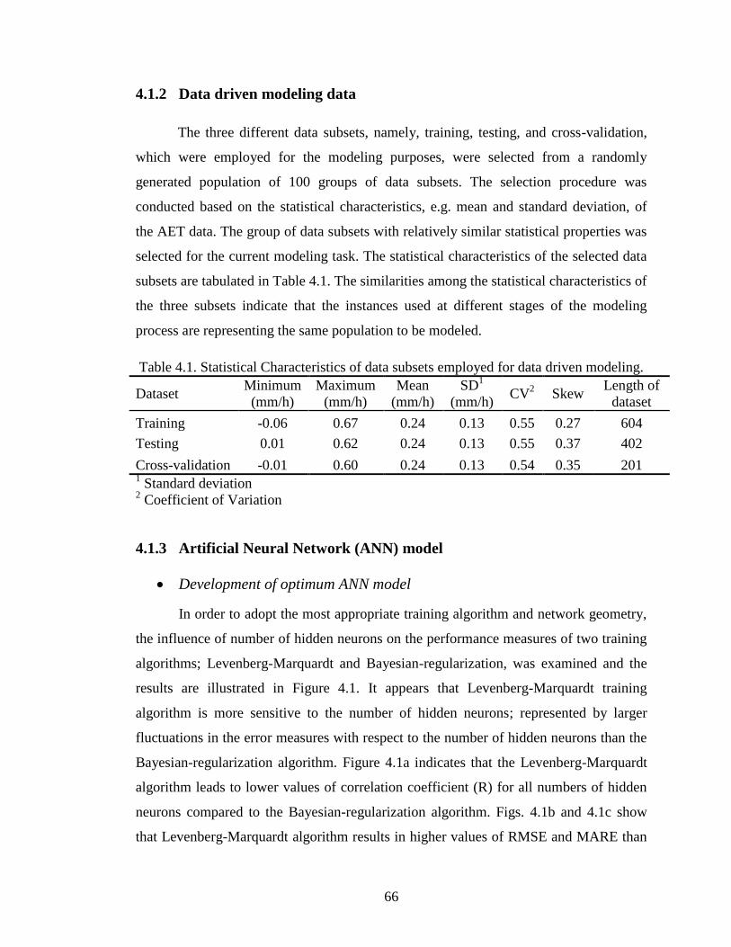
66

4.1.2 Data driven modeling data

The three different data subsets, namely, training, testing, and cross-validation,

which were employed for the modeling purposes, were selected from a randomly

generated population of 100 groups of data subsets. The selection procedure was

conducted based on the statistical characteristics, e.g. mean and standard deviation, of

the AET data. The group of data subsets with relatively similar statistical properties was

selected for the current modeling task. The statistical characteristics of the selected data

subsets are tabulated in Table 4.1. The similarities among the statistical characteristics of

the three subsets indicate that the instances used at different stages of the modeling

process are representing the same population to be modeled.

Table 4.1. Statistical Characteristics of data subsets employed for data driven modeling.

Dataset Minimum

(mm/h)

Maximum

(mm/h)

Mean

(mm/h)

SD1

(mm/h) CV

2 Skew

Length of

dataset

Training -0.06 0.67 0.24 0.13 0.55 0.27 604

Testing 0.01 0.62 0.24 0.13 0.55 0.37 402

Cross-validation -0.01 0.60 0.24 0.13 0.54 0.35 201 1 Standard deviation

2 Coefficient of Variation

4.1.3 Artificial Neural Network (ANN) model

Development of optimum ANN model

In order to adopt the most appropriate training algorithm and network geometry,

the influence of number of hidden neurons on the performance measures of two training

algorithms; Levenberg-Marquardt and Bayesian-regularization, was examined and the

results are illustrated in Figure 4.1. It appears that Levenberg-Marquardt training

algorithm is more sensitive to the number of hidden neurons; represented by larger

fluctuations in the error measures with respect to the number of hidden neurons than the

Bayesian-regularization algorithm. Figure 4.1a indicates that the Levenberg-Marquardt

algorithm leads to lower values of correlation coefficient (R) for all numbers of hidden

neurons compared to the Bayesian-regularization algorithm. Figs. 4.1b and 4.1c show

that Levenberg-Marquardt algorithm results in higher values of RMSE and MARE than

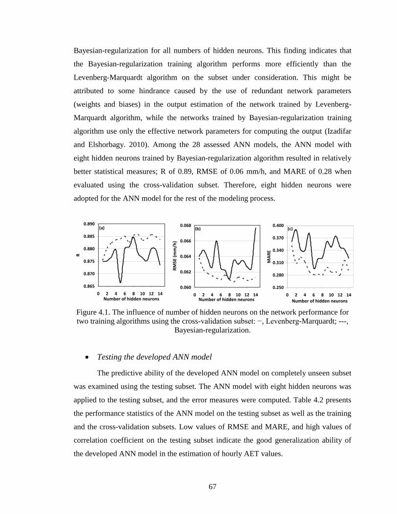
67

Bayesian-regularization for all numbers of hidden neurons. This finding indicates that

the Bayesian-regularization training algorithm performs more efficiently than the

Levenberg-Marquardt algorithm on the subset under consideration. This might be

attributed to some hindrance caused by the use of redundant network parameters

(weights and biases) in the output estimation of the network trained by Levenberg-

Marquardt algorithm, while the networks trained by Bayesian-regularization training

algorithm use only the effective network parameters for computing the output (Izadifar

and Elshorbagy. 2010). Among the 28 assessed ANN models, the ANN model with

eight hidden neurons trained by Bayesian-regularization algorithm resulted in relatively

better statistical measures; R of 0.89, RMSE of 0.06 mm/h, and MARE of 0.28 when

evaluated using the cross-validation subset. Therefore, eight hidden neurons were

adopted for the ANN model for the rest of the modeling process.

Figure 4.1. The influence of number of hidden neurons on the network performance for

two training algorithms using the cross-validation subset: −, Levenberg-Marquardt; ---,

Bayesian-regularization.

Testing the developed ANN model

The predictive ability of the developed ANN model on completely unseen subset

was examined using the testing subset. The ANN model with eight hidden neurons was

applied to the testing subset, and the error measures were computed. Table 4.2 presents

the performance statistics of the ANN model on the testing subset as well as the training

and the cross-validation subsets. Low values of RMSE and MARE, and high values of

correlation coefficient on the testing subset indicate the good generalization ability of

the developed ANN model in the estimation of hourly AET values.

0.250

0.280

0.310

0.340

0.370

0.400

0 2 4 6 8 10 12 14

Number of hidden neurons

MA

RE

0.060

0.062

0.064

0.066

0.068

0 2 4 6 8 10 12 14Number of hidden neurons

RM

SE (

mm

/h)

0.865

0.870

0.875

0.880

0.885

0.890

0 2 4 6 8 10 12 14Number of hidden neurons

R

(a) (b) (c)

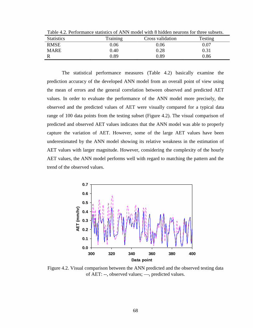
68

Table 4.2. Performance statistics of ANN model with 8 hidden neurons for three subsets.

Statistics Training Cross validation Testing

RMSE 0.06 0.06 0.07

MARE 0.40 0.28 0.31

R 0.89 0.89 0.86

The statistical performance measures (Table 4.2) basically examine the

prediction accuracy of the developed ANN model from an overall point of view using

the mean of errors and the general correlation between observed and predicted AET

values. In order to evaluate the performance of the ANN model more precisely, the

observed and the predicted values of AET were visually compared for a typical data

range of 100 data points from the testing subset (Figure 4.2). The visual comparison of

predicted and observed AET values indicates that the ANN model was able to properly

capture the variation of AET. However, some of the large AET values have been

underestimated by the ANN model showing its relative weakness in the estimation of

AET values with larger magnitude. However, considering the complexity of the hourly

AET values, the ANN model performs well with regard to matching the pattern and the

trend of the observed values.

Figure 4.2. Visual comparison between the ANN predicted and the observed testing data

of AET: --, observed values; , predicted values.

0.0

0.1

0.2

0.3

0.4

0.5

0.6

0.7

300 320 340 360 380 400

Data point

AE

T (

mm

/hr)

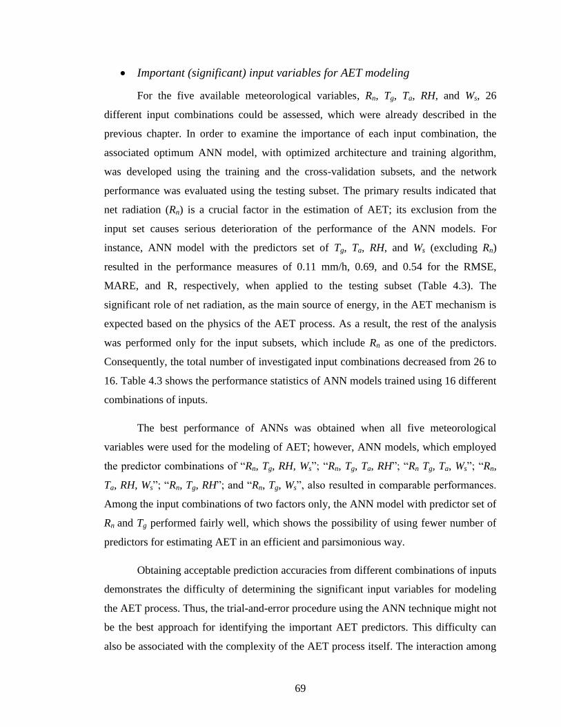
69

Important (significant) input variables for AET modeling

For the five available meteorological variables, Rn, Tg, Ta, RH, and Ws, 26

different input combinations could be assessed, which were already described in the

previous chapter. In order to examine the importance of each input combination, the

associated optimum ANN model, with optimized architecture and training algorithm,

was developed using the training and the cross-validation subsets, and the network

performance was evaluated using the testing subset. The primary results indicated that

net radiation (Rn) is a crucial factor in the estimation of AET; its exclusion from the

input set causes serious deterioration of the performance of the ANN models. For

instance, ANN model with the predictors set of Tg, Ta, RH, and Ws (excluding Rn)

resulted in the performance measures of 0.11 mm/h, 0.69, and 0.54 for the RMSE,

MARE, and R, respectively, when applied to the testing subset (Table 4.3). The

significant role of net radiation, as the main source of energy, in the AET mechanism is

expected based on the physics of the AET process. As a result, the rest of the analysis

was performed only for the input subsets, which include Rn as one of the predictors.

Consequently, the total number of investigated input combinations decreased from 26 to

16. Table 4.3 shows the performance statistics of ANN models trained using 16 different

combinations of inputs.

The best performance of ANNs was obtained when all five meteorological

variables were used for the modeling of AET; however, ANN models, which employed

the predictor combinations of ―Rn, Tg, RH, Ws‖; ―Rn, Tg, Ta, RH‖; ―Rn Tg, Ta, Ws‖; ―Rn,

Ta, RH, Ws‖; ―Rn, Tg, RH‖; and ―Rn, Tg, Ws‖, also resulted in comparable performances.

Among the input combinations of two factors only, the ANN model with predictor set of

Rn and Tg performed fairly well, which shows the possibility of using fewer number of

predictors for estimating AET in an efficient and parsimonious way.

Obtaining acceptable prediction accuracies from different combinations of inputs

demonstrates the difficulty of determining the significant input variables for modeling

the AET process. Thus, the trial-and-error procedure using the ANN technique might not

be the best approach for identifying the important AET predictors. This difficulty can

also be associated with the complexity of the AET process itself. The interaction among

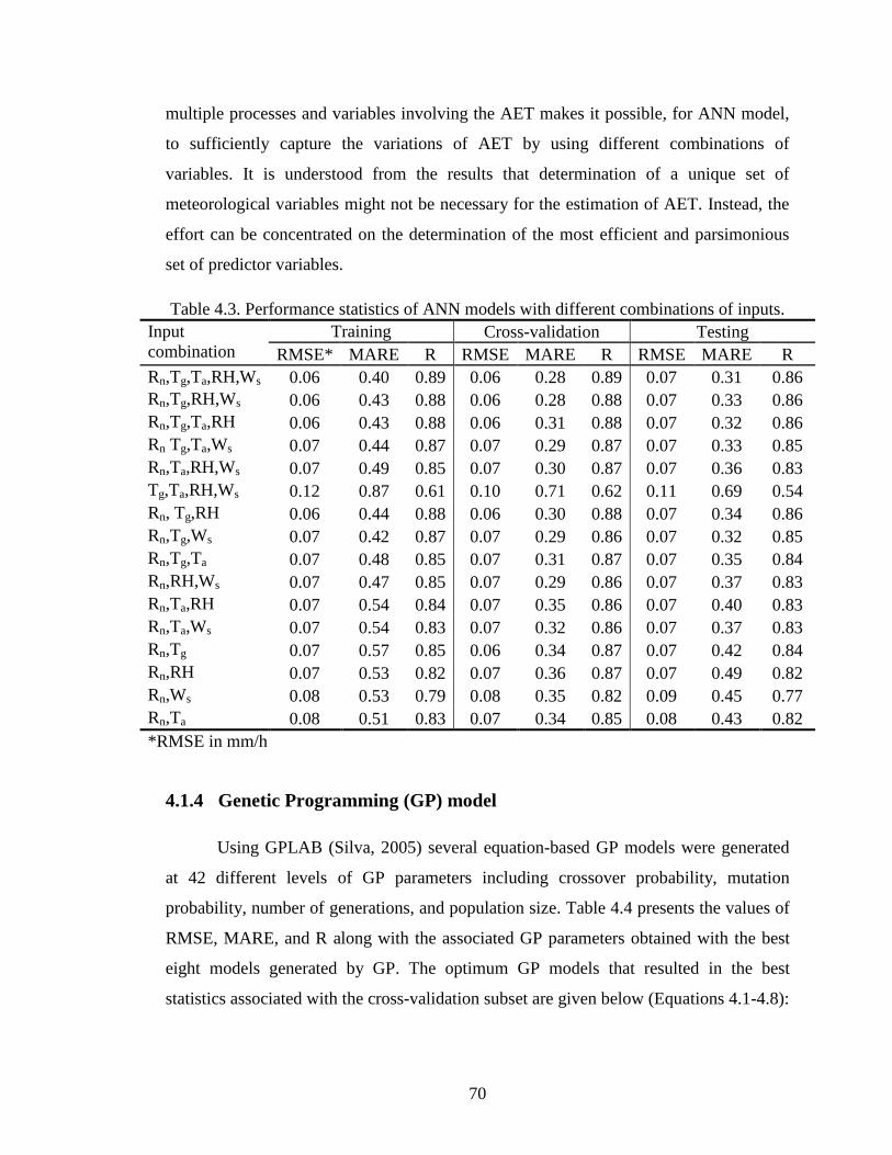
70

multiple processes and variables involving the AET makes it possible, for ANN model,

to sufficiently capture the variations of AET by using different combinations of

variables. It is understood from the results that determination of a unique set of

meteorological variables might not be necessary for the estimation of AET. Instead, the

effort can be concentrated on the determination of the most efficient and parsimonious

set of predictor variables.

Table 4.3. Performance statistics of ANN models with different combinations of inputs.

Input

combination

Training Cross-validation Testing

RMSE* MARE R RMSE MARE R RMSE MARE R

Rn,Tg,Ta,RH,Ws 0.06 0.40 0.89 0.06 0.28 0.89 0.07 0.31 0.86

Rn,Tg,RH,Ws 0.06 0.43 0.88 0.06 0.28 0.88 0.07 0.33 0.86

Rn,Tg,Ta,RH 0.06 0.43 0.88 0.06 0.31 0.88 0.07 0.32 0.86

Rn Tg,Ta,Ws 0.07 0.44 0.87 0.07 0.29 0.87 0.07 0.33 0.85

Rn,Ta,RH,Ws 0.07 0.49 0.85 0.07 0.30 0.87 0.07 0.36 0.83

Tg,Ta,RH,Ws 0.12 0.87 0.61 0.10 0.71 0.62 0.11 0.69 0.54

Rn, Tg,RH 0.06 0.44 0.88 0.06 0.30 0.88 0.07 0.34 0.86

Rn,Tg,Ws 0.07 0.42 0.87 0.07 0.29 0.86 0.07 0.32 0.85

Rn,Tg,Ta 0.07 0.48 0.85 0.07 0.31 0.87 0.07 0.35 0.84

Rn,RH,Ws 0.07 0.47 0.85 0.07 0.29 0.86 0.07 0.37 0.83

Rn,Ta,RH 0.07 0.54 0.84 0.07 0.35 0.86 0.07 0.40 0.83

Rn,Ta,Ws 0.07 0.54 0.83 0.07 0.32 0.86 0.07 0.37 0.83

Rn,Tg 0.07 0.57 0.85 0.06 0.34 0.87 0.07 0.42 0.84

Rn,RH 0.07 0.53 0.82 0.07 0.36 0.87 0.07 0.49 0.82

Rn,Ws 0.08 0.53 0.79 0.08 0.35 0.82 0.09 0.45 0.77

Rn,Ta 0.08 0.51 0.83 0.07 0.34 0.85 0.08 0.43 0.82

*RMSE in mm/h

4.1.4 Genetic Programming (GP) model

Using GPLAB (Silva, 2005) several equation-based GP models were generated

at 42 different levels of GP parameters including crossover probability, mutation

probability, number of generations, and population size. Table 4.4 presents the values of

RMSE, MARE, and R along with the associated GP parameters obtained with the best

eight models generated by GP. The optimum GP models that resulted in the best

statistics associated with the cross-validation subset are given below (Equations 4.1-4.8):

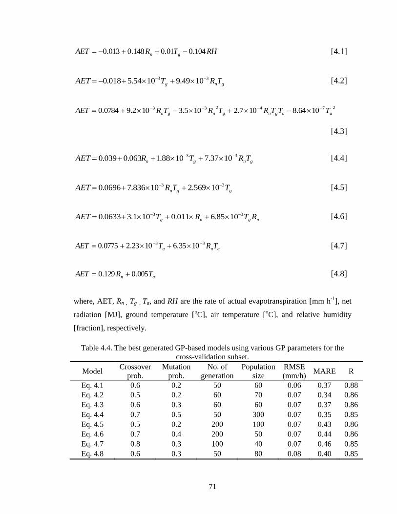
71

RHTRAET gn 104.001.0148.0013.0 [4.1]

gng TRTAET 33 1049.91054.5018.0 [4.2]

274233 1064.8107.2105.3102.90784.0 aagngngn TTTRTRTRAET

[4.3]

gngn TRTRAET 33 1037.71088.1063.0039.0

[4.4]

ggn TTRAET 33 10569.210836.70696.0 [4.5]

ngng RTRTAET 33 1085.6011.0101.30633.0 [4.6]

ana TRTAET 33 1035.61023.20775.0 [4.7]

an TRAET 005.0129.0 [4.8]

where, AET, Rn , Tg , Ta, and RH are the rate of actual evapotranspiration [mm h-1

], net

radiation [MJ], ground temperature [oC], air temperature [

oC], and relative humidity

[fraction], respectively.

Table 4.4. The best generated GP-based models using various GP parameters for the

cross-validation subset.

Model Crossover

prob.

Mutation

prob.

No. of

generation

Population

size

RMSE

(mm/h) MARE R

Eq. 4.1 0.6 0.2 50 60 0.06 0.37 0.88

Eq. 4.2 0.5 0.2 60 70 0.07 0.34 0.86

Eq. 4.3 0.6 0.3 60 60 0.07 0.37 0.86

Eq. 4.4 0.7 0.5 50 300 0.07 0.35 0.85

Eq. 4.5 0.5 0.2 200 100 0.07 0.43 0.86

Eq. 4.6 0.7 0.4 200 50 0.07 0.44 0.86

Eq. 4.7 0.8 0.3 100 40 0.07 0.46 0.85

Eq. 4.8 0.6 0.3 50 80 0.08 0.40 0.85

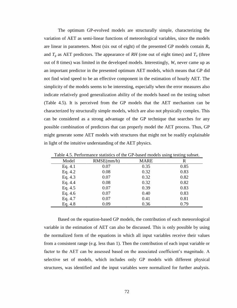
72

The optimum GP-evolved models are structurally simple, characterizing the

variation of AET as semi-linear functions of meteorological variables, since the models

are linear in parameters. Most (six out of eight) of the presented GP models contain Rn

and Tg as AET predictors. The appearance of RH (one out of eight times) and Ta (three

out of 8 times) was limited in the developed models. Interestingly, Ws never came up as

an important predictor in the presented optimum AET models, which means that GP did

not find wind speed to be an effective component in the estimation of hourly AET. The

simplicity of the models seems to be interesting, especially when the error measures also

indicate relatively good generalization ability of the models based on the testing subset

(Table 4.5). It is perceived from the GP models that the AET mechanism can be

characterized by structurally simple models, which are also not physically complex. This

can be considered as a strong advantage of the GP technique that searches for any

possible combination of predictors that can properly model the AET process. Thus, GP

might generate some AET models with structures that might not be readily explainable

in light of the intuitive understanding of the AET physics.

Table 4.5. Performance statistics of the GP-based models using testing subset.

Model RMSE(mm/h) MARE R

Eq. 4.1 0.07 0.35 0.85

Eq. 4.2 0.08 0.32 0.83

Eq. 4.3 0.07 0.32 0.82

Eq. 4.4 0.08 0.32 0.82

Eq. 4.5 0.07 0.39 0.83

Eq. 4.6 0.07 0.40 0.83

Eq. 4.7 0.07 0.41 0.81

Eq. 4.8 0.09 0.36 0.79

Based on the equation-based GP models, the contribution of each meteorological

variable in the estimation of AET can also be discussed. This is only possible by using

the normalized form of the equations in which all input variables receive their values

from a consistent range (e.g. less than 1). Then the contribution of each input variable or

factor to the AET can be assessed based on the associated coefficient’s magnitude. A

selective set of models, which includes only GP models with different physical

structures, was identified and the input variables were normalized for further analysis.

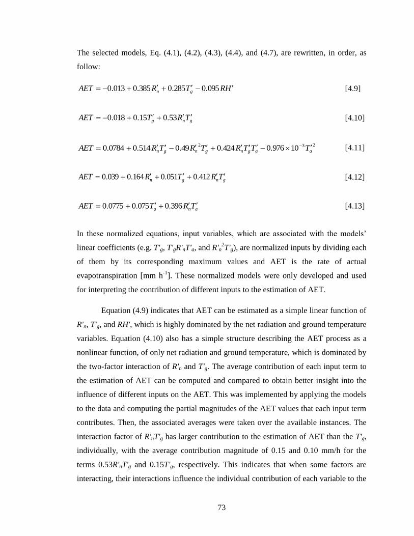
73

The selected models, Eq. (4.1), (4.2), (4.3), (4.4), and (4.7), are rewritten, in order, as

follow:

HRTRAET gn 095.0285.0385.0013.0 [4.9]

gng TRTAET 53.015.0018.0 [4.10]

23210976.0424.049.0514.00784.0 aagngngn TTTRTRTRAET [4.11]

gngn TRTRAET 412.0051.0164.0039.0 [4.12]

ana TRTAET 396.0075.00775.0 [4.13]

In these normalized equations, input variables, which are associated with the models’

linear coefficients (e.g. T'g, T'gR'nT'a, and R'n2T'g), are normalized inputs by dividing each

of them by its corresponding maximum values and AET is the rate of actual

evapotranspiration [mm h-1

]. These normalized models were only developed and used

for interpreting the contribution of different inputs to the estimation of AET.

Equation (4.9) indicates that AET can be estimated as a simple linear function of

R'n, T'g, and RH', which is highly dominated by the net radiation and ground temperature

variables. Equation (4.10) also has a simple structure describing the AET process as a

nonlinear function, of only net radiation and ground temperature, which is dominated by

the two-factor interaction of R'n and T'g. The average contribution of each input term to

the estimation of AET can be computed and compared to obtain better insight into the

influence of different inputs on the AET. This was implemented by applying the models

to the data and computing the partial magnitudes of the AET values that each input term

contributes. Then, the associated averages were taken over the available instances. The

interaction factor of R'nT'g has larger contribution to the estimation of AET than the T'g,

individually, with the average contribution magnitude of 0.15 and 0.10 mm/h for the

terms 0.53R'nT'g and 0.15T'g, respectively. This indicates that when some factors are

interacting, their interactions influence the individual contribution of each variable to the

74

AET mechanism. Consequently, the interaction term (factor) is more responsible for

AET variations than the individual variables. In Eq. (4.11), the air temperature (T'a)

variable has been included in addition to the R'n and T'g. The air temperature has

appeared both as an individual variable and as an interacting factor in the three-factor

interaction term of R'nT'gT'a. According to the coefficients associated with these

variables in Eq. (4.11), T'a can affect the rate of AET only through the influence it might

have on the R'n and T'g (interacting coefficient of 0.424 compared to that of air

temperature, 0.000976). The structure of Eq. (4.12) also confirms the importance of

interaction effects of multiple variables rather than the individual processes. The

combined component of R'nT'g is more responsible for the variation of AET than the R'n

and T'g individually. The average contribution magnitude of each of the terms

0.412R'nT'g, 0.164R'n, and 0.051T'g in the estimation of AET values are 0.12, 0.05, and

0.03 mm/h, respectively. Equation (4.13) demonstrates that the AET mechanism can

even be characterized as a simple semi-linear function of R'n and T'a only, which are

commonly available meteorological measurements. Again, the AET model is dominated

by the interaction factor of the two variables. The interaction and individual terms of

0.396R'nT'a and 0.075T'a are contributing to the estimation of AET by the average

magnitude of 0.11 and 0.05 mm/h, respectively.

Although the generated models, based on error measures, are performing well

and relatively similar, they are using different combinations of inputs with different

mathematical structures. This demonstrates that precise identification of the

meteorological variables driving the AET process is not an easy and straightforward

task, where different combinations of inputs may result in relatively good AET

estimation (Izadifar and Elshorbagy, 2010). The results obtained from the GP-evolved

models indicate that the hourly AET process can be estimated by both linear and

nonlinear relationships. The prediction accuracy of the AET models, using the GP

technique, could vary within a possible range of 0.07 to 0.09 (mm/h), 0.32 to 0.41, and

0.79 to 0.85 for RMSE, MARE and R, respectively. Using the above-listed GP models,

one may choose one of them for estimating the rate of AET based on the meteorological

data that are available. Thus, the proposed GP models can suit different conditions of

data availability.

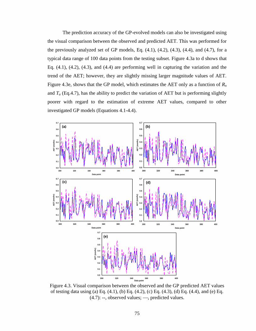
75

The prediction accuracy of the GP-evolved models can also be investigated using

the visual comparison between the observed and predicted AET. This was performed for

the previously analyzed set of GP models, Eq. (4.1), (4.2), (4.3), (4.4), and (4.7), for a

typical data range of 100 data points from the testing subset. Figure 4.3a to d shows that

Eq. (4.1), (4.2), (4.3), and (4.4) are performing well in capturing the variation and the

trend of the AET; however, they are slightly missing larger magnitude values of AET.

Figure 4.3e, shows that the GP model, which estimates the AET only as a function of Rn

and Ta (Eq.4.7), has the ability to predict the variation of AET but is performing slightly

poorer with regard to the estimation of extreme AET values, compared to other

investigated GP models (Equations 4.1-4.4).

Figure 4.3. Visual comparison between the observed and the GP predicted AET values

of testing data using (a) Eq. (4.1), (b) Eq. (4.2), (c) Eq. (4.3), (d) Eq. (4.4), and (e) Eq.

(4.7): --, observed values; , predicted values.

0.0

0.1

0.2

0.3

0.4

0.5

0.6

0.7

300 320 340 360 380 400

Data point

AE

T (

mm

/hr)

0.0

0.1

0.2

0.3

0.4

0.5

0.6

0.7

300 320 340 360 380 400

Data point

AE

T (

mm

/hr)

(b)(a)

0.0

0.1

0.2

0.3

0.4

0.5

0.6

0.7

300 320 340 360 380 400

Data point

AE

T (

mm

/hr)

(c)

0.0

0.1

0.2

0.3

0.4

0.5

0.6

0.7

300 320 340 360 380 400

Data point

AE

T (

mm

/hr)

(d)

0.0

0.1

0.2

0.3

0.4

0.5

0.6

0.7

300 320 340 360 380 400Data point

AE

T (

mm

/hr)

(e)

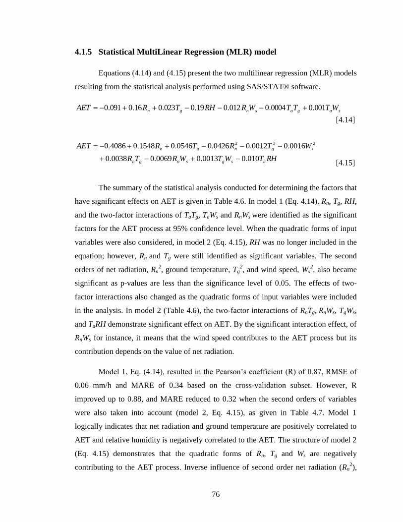
76

4.1.5 Statistical MultiLinear Regression (MLR) model

Equations (4.14) and (4.15) present the two multilinear regression (MLR) models

resulting from the statistical analysis performed using SAS/STAT® software.

sagasngn WTTTWRRHTRAET 001.00004.0012.019.0023.016.0091.0

[4.14]

[4.15]

The summary of the statistical analysis conducted for determining the factors that

have significant effects on AET is given in Table 4.6. In model 1 (Eq. 4.14), Rn, Tg, RH,

and the two-factor interactions of TaTg, TaWs and RnWs were identified as the significant

factors for the AET process at 95% confidence level. When the quadratic forms of input

variables were also considered, in model 2 (Eq. 4.15), RH was no longer included in the

equation; however, Rn and Tg were still identified as significant variables. The second

orders of net radiation, Rn2, ground temperature, Tg

2, and wind speed, Ws

2, also became

significant as p-values are less than the significance level of 0.05. The effects of two-

factor interactions also changed as the quadratic forms of input variables were included

in the analysis. In model 2 (Table 4.6), the two-factor interactions of RnTg, RnWs, TgWs,

and TaRH demonstrate significant effect on AET. By the significant interaction effect, of

RnWs for instance, it means that the wind speed contributes to the AET process but its

contribution depends on the value of net radiation.

Model 1, Eq. (4.14), resulted in the Pearson’s coefficient (R) of 0.87, RMSE of

0.06 mm/h and MARE of 0.34 based on the cross-validation subset. However, R

improved up to 0.88, and MARE reduced to 0.32 when the second orders of variables

were also taken into account (model 2, Eq. 4.15), as given in Table 4.7. Model 1

logically indicates that net radiation and ground temperature are positively correlated to

AET and relative humidity is negatively correlated to the AET. The structure of model 2

(Eq. 4.15) demonstrates that the quadratic forms of Rn, Tg and Ws are negatively

contributing to the AET process. Inverse influence of second order net radiation (Rn2),

RHTWTWRTR

WTRTRAET

asgsngn

sgngn

010.00013.00069.00038.0

0016.00012.00426.00546.01548.04086.0 222

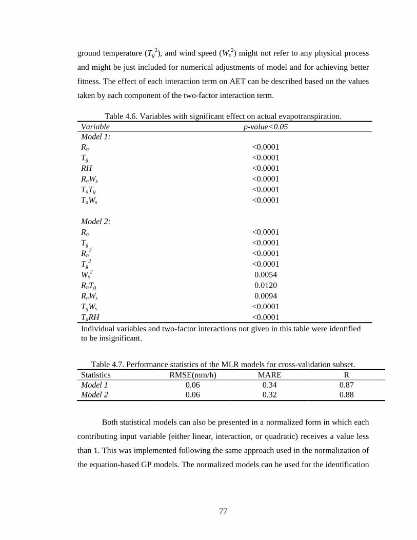
77

ground temperature (Tg2), and wind speed (Ws

2) might not refer to any physical process

and might be just included for numerical adjustments of model and for achieving better

fitness. The effect of each interaction term on AET can be described based on the values

taken by each component of the two-factor interaction term.

Table 4.6. Variables with significant effect on actual evapotranspiration.

Variable p-value<0.05

Model 1:

Rn <0.0001

Tg <0.0001

RH <0.0001

RnWs <0.0001

TaTg <0.0001

TaWs <0.0001

Model 2:

Rn <0.0001

Tg <0.0001

Rn2 <0.0001

Tg2 <0.0001

Ws2 0.0054

RnTg 0.0120

RnWs 0.0094

TgWs <0.0001

TaRH <0.0001

Individual variables and two-factor interactions not given in this table were identified

to be insignificant.

Table 4.7. Performance statistics of the MLR models for cross-validation subset.

Statistics RMSE(mm/h) MARE R

Model 1 0.06 0.34 0.87

Model 2 0.06 0.32 0.88

Both statistical models can also be presented in a normalized form in which each

contributing input variable (either linear, interaction, or quadratic) receives a value less

than 1. This was implemented following the same approach used in the normalization of

the equation-based GP models. The normalized models can be used for the identification

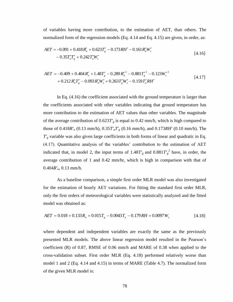
78

of variables having more contribution, to the estimation of AET, than others. The

normalized form of the regression models (Eq. 4.14 and Eq. 4.15) are given, in order, as:

saga

sngn

WTTT

WRHRTRAET

242.035.0

161.0173.0623.0418.0091.0 [4.16]

HRTWTWRTR

WTRTRAET

asgsngn

sgngn

159.0263.0093.0212.0

123.0881.0289.048.1404.0409.02 22

[4.17]

In Eq. (4.16) the coefficient associated with the ground temperature is larger than

the coefficients associated with other variables indicating that ground temperature has

more contribution to the estimation of AET values than other variables. The magnitude

of the average contribution of 0.623T'g is equal to 0.42 mm/h, which is high compared to

those of 0.418R'n (0.13 mm/h), 0.35T'aT'g (0.16 mm/h), and 0.173RH' (0.10 mm/h). The

T'g variable was also given large coefficients in both forms of linear and quadratic in Eq.

(4.17). Quantitative analysis of the variables’ contribution to the estimation of AET

indicated that, in model 2, the input terms of 1.48T'g and 0.881T'g2 have, in order, the

average contribution of 1 and 0.42 mm/hr, which is high in comparison with that of

0.404R'n, 0.13 mm/h.

As a baseline comparison, a simple first order MLR model was also investigated

for the estimation of hourly AET variations. For fitting the standard first order MLR,

only the first orders of meteorological variables were statistically analyzed and the fitted

model was obtained as:

sagn WRHTTRAET 0097.0179.00043.0015.0133.0018.0 [4.18]

where dependent and independent variables are exactly the same as the previously

presented MLR models. The above linear regression model resulted in the Pearson’s

coefficient (R) of 0.87, RMSE of 0.06 mm/h and MARE of 0.38 when applied to the

cross-validation subset. First order MLR (Eq. 4.18) performed relatively worse than

model 1 and 2 (Eq. 4.14 and 4.15) in terms of MARE (Table 4.7). The normalized form

of the given MLR model is:

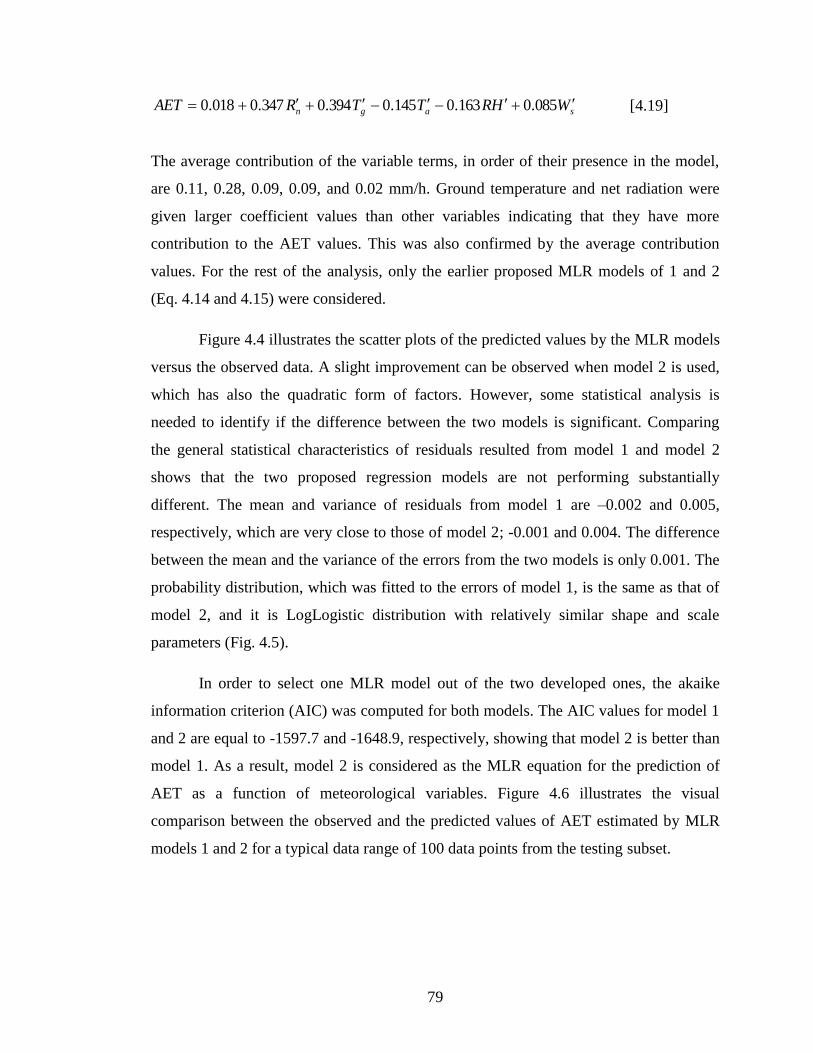
79

sagn WHRTTRAET 085.0163.0145.0394.0347.0018.0 [4.19]

The average contribution of the variable terms, in order of their presence in the model,

are 0.11, 0.28, 0.09, 0.09, and 0.02 mm/h. Ground temperature and net radiation were

given larger coefficient values than other variables indicating that they have more

contribution to the AET values. This was also confirmed by the average contribution

values. For the rest of the analysis, only the earlier proposed MLR models of 1 and 2

(Eq. 4.14 and 4.15) were considered.

Figure 4.4 illustrates the scatter plots of the predicted values by the MLR models

versus the observed data. A slight improvement can be observed when model 2 is used,

which has also the quadratic form of factors. However, some statistical analysis is

needed to identify if the difference between the two models is significant. Comparing

the general statistical characteristics of residuals resulted from model 1 and model 2

shows that the two proposed regression models are not performing substantially

different. The mean and variance of residuals from model 1 are –0.002 and 0.005,

respectively, which are very close to those of model 2; -0.001 and 0.004. The difference

between the mean and the variance of the errors from the two models is only 0.001. The

probability distribution, which was fitted to the errors of model 1, is the same as that of

model 2, and it is LogLogistic distribution with relatively similar shape and scale

parameters (Fig. 4.5).

In order to select one MLR model out of the two developed ones, the akaike

information criterion (AIC) was computed for both models. The AIC values for model 1

and 2 are equal to -1597.7 and -1648.9, respectively, showing that model 2 is better than

model 1. As a result, model 2 is considered as the MLR equation for the prediction of

AET as a function of meteorological variables. Figure 4.6 illustrates the visual

comparison between the observed and the predicted values of AET estimated by MLR

models 1 and 2 for a typical data range of 100 data points from the testing subset.

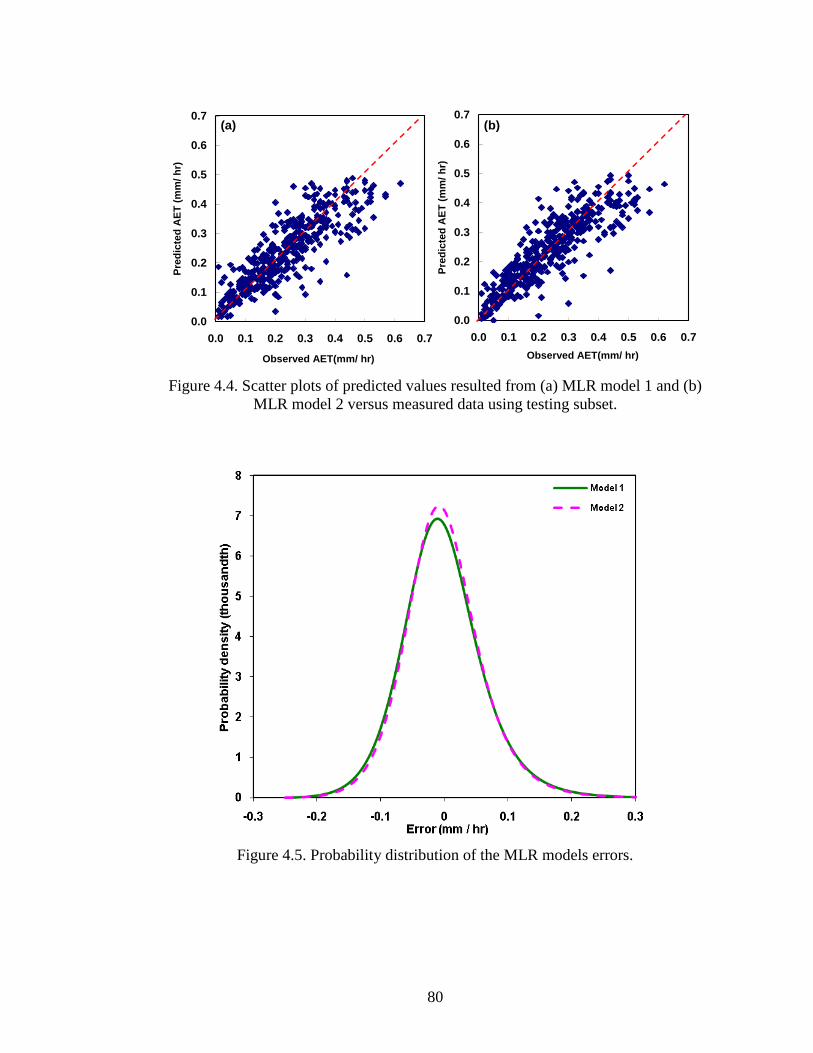
80

Figure 4.4. Scatter plots of predicted values resulted from (a) MLR model 1 and (b)

MLR model 2 versus measured data using testing subset.

Figure 4.5. Probability distribution of the MLR models errors.

0.0

0.1

0.2

0.3

0.4

0.5

0.6

0.7

0.0 0.1 0.2 0.3 0.4 0.5 0.6 0.7

Observed AET(mm/ hr)

Pre

dic

ted

AE

T (

mm

/ h

r)

0.0

0.1

0.2

0.3

0.4

0.5

0.6

0.7

0.0 0.1 0.2 0.3 0.4 0.5 0.6 0.7


Pre

dic

ted

AE

T (

mm

/ h

r)

(a) (b)

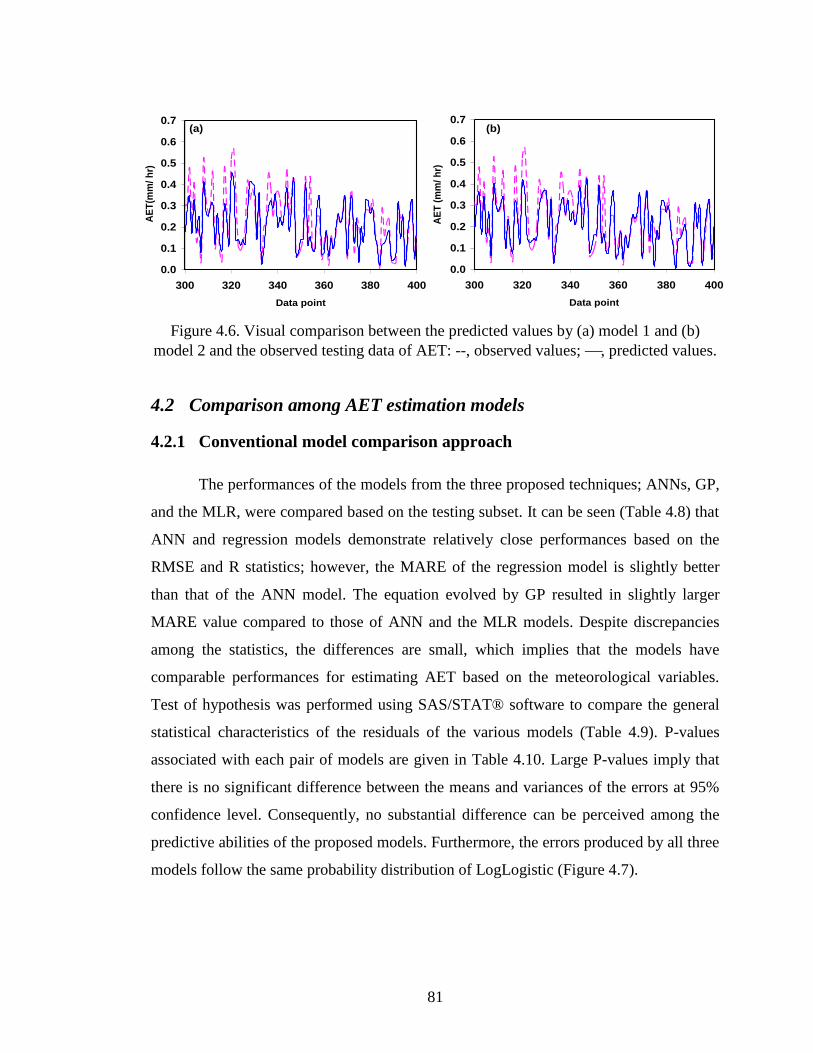
81

Figure 4.6. Visual comparison between the predicted values by (a) model 1 and (b)

model 2 and the observed testing data of AET: --, observed values; , predicted values.

4.2 Comparison among AET estimation models

4.2.1 Conventional model comparison approach

The performances of the models from the three proposed techniques; ANNs, GP,

and the MLR, were compared based on the testing subset. It can be seen (Table 4.8) that

ANN and regression models demonstrate relatively close performances based on the

RMSE and R statistics; however, the MARE of the regression model is slightly better

than that of the ANN model. The equation evolved by GP resulted in slightly larger

MARE value compared to those of ANN and the MLR models. Despite discrepancies

among the statistics, the differences are small, which implies that the models have

comparable performances for estimating AET based on the meteorological variables.

Test of hypothesis was performed using SAS/STAT® software to compare the general

statistical characteristics of the residuals of the various models (Table 4.9). P-values

associated with each pair of models are given in Table 4.10. Large P-values imply that

there is no significant difference between the means and variances of the errors at 95%

confidence level. Consequently, no substantial difference can be perceived among the

predictive abilities of the proposed models. Furthermore, the errors produced by all three

models follow the same probability distribution of LogLogistic (Figure 4.7).

0.0

0.1

0.2

0.3

0.4

0.5

0.6

0.7

300 320 340 360 380 400

Data point

AE

T(m

m/

hr)

0.0

0.1

0.2

0.3

0.4

0.5

0.6

0.7

300 320 340 360 380 400

Data point

AE

T (

mm

/ h

r)

(a) (b)

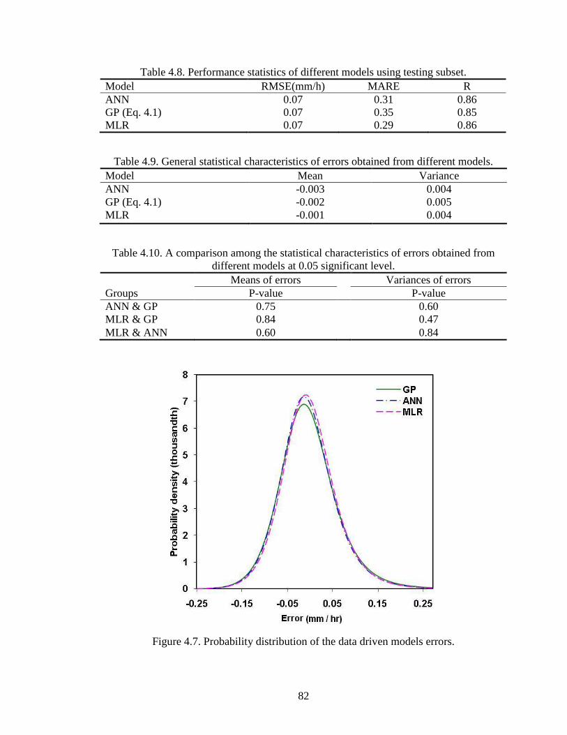
82

Table 4.8. Performance statistics of different models using testing subset.


ANN 0.07 0.31 0.86

GP (Eq. 4.1) 0.07 0.35 0.85

MLR 0.07 0.29 0.86

Table 4.9. General statistical characteristics of errors obtained from different models.

Model Mean Variance

ANN -0.003 0.004

GP (Eq. 4.1) -0.002 0.005

MLR -0.001 0.004

Table 4.10. A comparison among the statistical characteristics of errors obtained from

different models at 0.05 significant level.

Means of errors Variances of errors

Groups P-value P-value

ANN & GP 0.75 0.60

MLR & GP 0.84 0.47

MLR & ANN 0.60 0.84

Figure 4.7. Probability distribution of the data driven models errors.

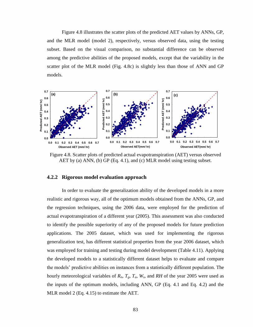
83

Figure 4.8 illustrates the scatter plots of the predicted AET values by ANNs, GP,

and the MLR model (model 2), respectively, versus observed data, using the testing

subset. Based on the visual comparison, no substantial difference can be observed

among the predictive abilities of the proposed models, except that the variability in the

scatter plot of the MLR model (Fig. 4.8c) is slightly less than those of ANN and GP

models.


AET by (a) ANN, (b) GP (Eq. 4.1), and (c) MLR model using testing subset.

4.2.2 Rigorous model evaluation approach

In order to evaluate the generalization ability of the developed models in a more

realistic and rigorous way, all of the optimum models obtained from the ANNs, GP, and

the regression techniques, using the 2006 data, were employed for the prediction of

actual evapotranspiration of a different year (2005). This assessment was also conducted

to identify the possible superiority of any of the proposed models for future prediction

applications. The 2005 dataset, which was used for implementing the rigorous

generalization test, has different statistical properties from the year 2006 dataset, which

was employed for training and testing during model development (Table 4.11). Applying

the developed models to a statistically different dataset helps to evaluate and compare

the models’ predictive abilities on instances from a statistically different population. The

hourly meteorological variables of Rn, Tg, Ta, Ws, and RH of the year 2005 were used as

the inputs of the optimum models, including ANN, GP (Eq. 4.1 and Eq. 4.2) and the

MLR model 2 (Eq. 4.15) to estimate the AET.

0.0

0.1

0.2

0.3

0.4

0.5

0.6

0.7

0.0 0.1 0.2 0.3 0.4 0.5 0.6 0.7

Observed AET (mm/ hr)

Pre

dic

ted

AE

T (

mm

/ h

r)

0.0

0.1

0.2

0.3

0.4

0.5

0.6

0.7

0.0 0.1 0.2 0.3 0.4 0.5 0.6 0.7


Pre

dic

ted

AE

T (

mm

/ h

r)

0.0

0.1

0.2

0.3

0.4

0.5

0.6

0.7

0.0 0.1 0.2 0.3 0.4 0.5 0.6 0.7


Pre

dic

ted

AE

T (

mm

/ h

r)

(a) (b) (c)

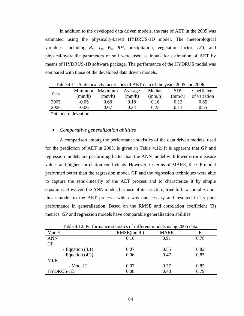
84

In addition to the developed data driven models, the rate of AET in the 2005 was

estimated using the physically-based HYDRUS-1D model. The meteorological

variables, including Rn, Ta, Ws, RH, precipitation, vegetation factor, LAI, and

physical/hydraulic parameters of soil were used as inputs for estimation of AET by

means of HYDRUS-1D software package. The performance of the HYDRUS model was

compared with those of the developed data driven models.

Table 4.11. Statistical characteristics of AET data of the years 2005 and 2006.

Year Minimum

(mm/h)

Maximum

(mm/h)

Average

(mm/h)

Median

(mm/h)

SD*

(mm/h)

Coefficient

of variation

2005 -0.05 0.68 0.18 0.16 0.12 0.65

2006 -0.06 0.67 0.24 0.23 0.13 0.55

*Standard deviation

Comparative generalization abilities

A comparison among the performance statistics of the data driven models, used

for the prediction of AET in 2005, is given in Table 4.12. It is apparent that GP and

regression models are performing better than the ANN model with lower error measure

values and higher correlation coefficients. However, in terms of MARE, the GP model

performed better than the regression model. GP and the regression techniques were able

to capture the semi-linearity of the AET process and to characterize it by simple

equations. However, the ANN model, because of its structure, tried to fit a complex non-

linear model to the AET process, which was unnecessary and resulted in its poor

performance in generalization. Based on the RMSE and correlation coefficient (R)

metrics, GP and regression models have comparable generalization abilities.

Table 4.12. Performance statistics of different models using 2005 data.


ANN 0.10 0.91 0.78

GP

- Equation (4.1) 0.07 0.55 0.82

- Equation (4.2) 0.06 0.47 0.85

MLR

- Model 2 0.07 0.57 0.85

HYDRUS-1D 0.08 0.48 0.79

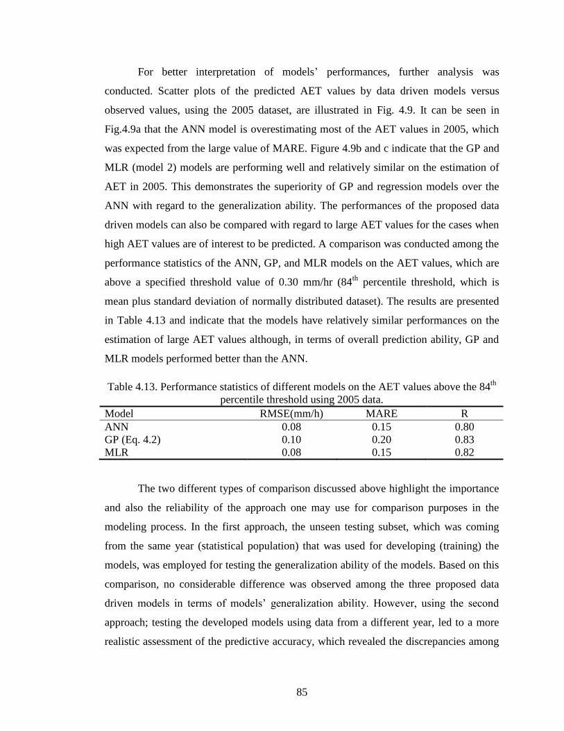
85

For better interpretation of models’ performances, further analysis was

conducted. Scatter plots of the predicted AET values by data driven models versus

observed values, using the 2005 dataset, are illustrated in Fig. 4.9. It can be seen in

Fig.4.9a that the ANN model is overestimating most of the AET values in 2005, which

was expected from the large value of MARE. Figure 4.9b and c indicate that the GP and

MLR (model 2) models are performing well and relatively similar on the estimation of

AET in 2005. This demonstrates the superiority of GP and regression models over the

ANN with regard to the generalization ability. The performances of the proposed data

driven models can also be compared with regard to large AET values for the cases when

high AET values are of interest to be predicted. A comparison was conducted among the

performance statistics of the ANN, GP, and MLR models on the AET values, which are

above a specified threshold value of 0.30 mm/hr (84th

percentile threshold, which is

mean plus standard deviation of normally distributed dataset). The results are presented

in Table 4.13 and indicate that the models have relatively similar performances on the

estimation of large AET values although, in terms of overall prediction ability, GP and

MLR models performed better than the ANN.

Table 4.13. Performance statistics of different models on the AET values above the 84th

percentile threshold using 2005 data.


ANN 0.08 0.15 0.80

GP (Eq. 4.2) 0.10 0.20 0.83

MLR 0.08 0.15 0.82

The two different types of comparison discussed above highlight the importance

and also the reliability of the approach one may use for comparison purposes in the

modeling process. In the first approach, the unseen testing subset, which was coming

from the same year (statistical population) that was used for developing (training) the

models, was employed for testing the generalization ability of the models. Based on this

comparison, no considerable difference was observed among the three proposed data

driven models in terms of models’ generalization ability. However, using the second

approach; testing the developed models using data from a different year, led to a more

realistic assessment of the predictive accuracy, which revealed the discrepancies among

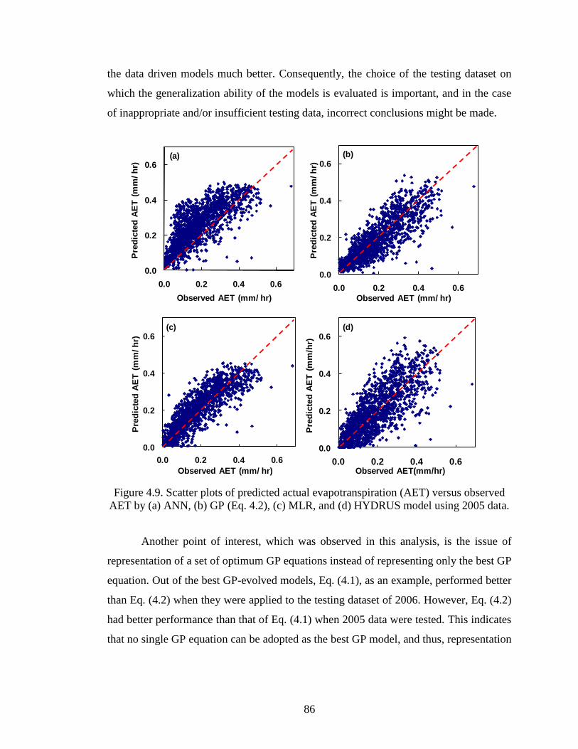
86

the data driven models much better. Consequently, the choice of the testing dataset on

which the generalization ability of the models is evaluated is important, and in the case

of inappropriate and/or insufficient testing data, incorrect conclusions might be made.


AET by (a) ANN, (b) GP (Eq. 4.2), (c) MLR, and (d) HYDRUS model using 2005 data.

Another point of interest, which was observed in this analysis, is the issue of

representation of a set of optimum GP equations instead of representing only the best GP

equation. Out of the best GP-evolved models, Eq. (4.1), as an example, performed better

than Eq. (4.2) when they were applied to the testing dataset of 2006. However, Eq. (4.2)

had better performance than that of Eq. (4.1) when 2005 data were tested. This indicates

that no single GP equation can be adopted as the best GP model, and thus, representation

0.0

0.2

0.4

0.6

0.0 0.2 0.4 0.6

Pre

dic

ted

AE

T (

mm

/ h

r)


0.0

0.2

0.4

0.6

0.0 0.2 0.4 0.6

Pre

dic

ted

AE

T (

mm

/ h

r)


0.0

0.2

0.4

0.6

0.0 0.2 0.4 0.6

Pre

dic

ted

AE

T (

mm

/ h

r)


(a) (b)

(c)

0.0

0.2

0.4

0.6

0.0 0.2 0.4 0.6

Pre

dic

ted

AE

T (

mm

/hr)

Observed AET(mm/hr)

(d)

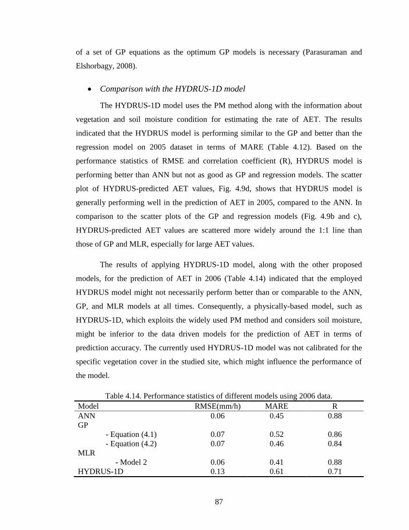
87

of a set of GP equations as the optimum GP models is necessary (Parasuraman and

Elshorbagy, 2008).

Comparison with the HYDRUS-1D model

The HYDRUS-1D model uses the PM method along with the information about

vegetation and soil moisture condition for estimating the rate of AET. The results

indicated that the HYDRUS model is performing similar to the GP and better than the

regression model on 2005 dataset in terms of MARE (Table 4.12). Based on the

performance statistics of RMSE and correlation coefficient (R), HYDRUS model is

performing better than ANN but not as good as GP and regression models. The scatter

plot of HYDRUS-predicted AET values, Fig. 4.9d, shows that HYDRUS model is

generally performing well in the prediction of AET in 2005, compared to the ANN. In

comparison to the scatter plots of the GP and regression models (Fig. 4.9b and c),

HYDRUS-predicted AET values are scattered more widely around the 1:1 line than

those of GP and MLR, especially for large AET values.

The results of applying HYDRUS-1D model, along with the other proposed

models, for the prediction of AET in 2006 (Table 4.14) indicated that the employed

HYDRUS model might not necessarily perform better than or comparable to the ANN,

GP, and MLR models at all times. Consequently, a physically-based model, such as

HYDRUS-1D, which exploits the widely used PM method and considers soil moisture,

might be inferior to the data driven models for the prediction of AET in terms of

prediction accuracy. The currently used HYDRUS-1D model was not calibrated for the

specific vegetation cover in the studied site, which might influence the performance of

the model.

Table 4.14. Performance statistics of different models using 2006 data.


ANN 0.06 0.45 0.88

GP

- Equation (4.1) 0.07 0.52 0.86

- Equation (4.2) 0.07 0.46 0.84

MLR

- Model 2 0.06 0.41 0.88

HYDRUS-1D 0.13 0.61 0.71

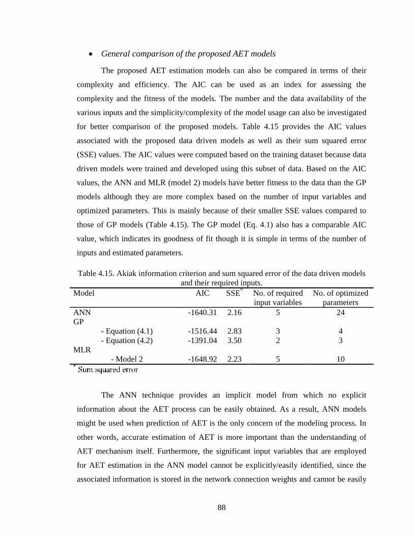
88

General comparison of the proposed AET models

The proposed AET estimation models can also be compared in terms of their

complexity and efficiency. The AIC can be used as an index for assessing the

complexity and the fitness of the models. The number and the data availability of the

various inputs and the simplicity/complexity of the model usage can also be investigated

for better comparison of the proposed models. Table 4.15 provides the AIC values

associated with the proposed data driven models as well as their sum squared error

(SSE) values. The AIC values were computed based on the training dataset because data

driven models were trained and developed using this subset of data. Based on the AIC

values, the ANN and MLR (model 2) models have better fitness to the data than the GP

models although they are more complex based on the number of input variables and

optimized parameters. This is mainly because of their smaller SSE values compared to

those of GP models (Table 4.15). The GP model (Eq. 4.1) also has a comparable AIC

value, which indicates its goodness of fit though it is simple in terms of the number of

inputs and estimated parameters.

Table 4.15. Akiak information criterion and sum squared error of the data driven models

and their required inputs.

Model AIC SSE No. of required

input variables

No. of optimized

parameters

ANN -1640.31 2.16 5 24

GP

- Equation (4.1) -1516.44 2.83 3 4

- Equation (4.2) -1391.04 3.50 2 3

MLR

- Model 2 -1648.92 2.23 5 10

The ANN technique provides an implicit model from which no explicit

information about the AET process can be easily obtained. As a result, ANN models

might be used when prediction of AET is the only concern of the modeling process. In

other words, accurate estimation of AET is more important than the understanding of

AET mechanism itself. Furthermore, the significant input variables that are employed

for AET estimation in the ANN model cannot be explicitly/easily identified, since the

associated information is stored in the network connection weights and cannot be easily

89

interpreted. For the end user, application of ANN models is also not as easy as the

equation-based models. The GP and MLR models are both equation-based models and

are of interest for hydrologists and modellers because of their transparency and

simplicity in application and usage. Explicit form of equation-based models, such as GP

and MLR, makes it possible to extract some information about the physics of the

process. The GP model has the advantage of using fewer input variables (Table 4.15)

and also has simpler and more realistic structure than the regression model.

Consequently, the GP model becomes more applicable when a limited number of

meteorological variables is available or can be measured. From this point of view, GP is

more efficient than the MLR for the prediction of AET. In addition, the simple structure

of the GP models makes it easy for the users to understand how input variables are

contributing to the AET process. This can also be achieved from the MLR equation;

however, it is not as easy as the GP model because of the structural complexity of the

MLR models.

The HYDRUS model that was employed for the estimation of AET required the

rainfall and LAI information, in addition to the meteorological variables used in the data

driven techniques. The information of LAI was measured in weekly basis and was

disaggregated to the hourly basis for consistency with the time resolution of other

variables. Disaggregation of data involves some uncertainty, which most probably has

been propagated to the estimated AET values. Indirect estimation of AET using the

HYDRUS model also introduces some uncertainty in the predictions. This is because the

AET is calculated from its partitioned components (actual evaporation and

transpiration), which are separately estimated using the standard PM model and

simulated soil moisture profile where the latter is also a source of uncertainty in the

model. These uncertainties, embedded in the estimated AET values, are considered as

disadvantage in the modeling process. In addition, requirement of additional input

variables, such as LAI and hourly rainfall, which are not readily available data for most

case studies, is considered also a disadvantage of HYDRUS model compared to the

proposed data driven models.

90

4.3 Wavelet analysis

4.3.1 Overview

Using the software package developed for MATLAB and provided on-line by

Grinsted et al. (2004), continuous wavelet transform of the meteorological variables

(predictors) and AET (predictand) time series was performed for identifying the

dominant temporal cyclic events. In addition to continuous wavelet transform, the cross

wavelet transform between each predictor variable and the AET signal was performed

for identifying the possible covariances, which represent the influence of the predictor

on the variations of AET. In general, the utility and applicability of WA were examined

for identifying, prior to the modeling, the important variables that influence the hourly

AET, and also to improve the understanding of the AET mechanism. In the following

sections, the results and discussions will mainly focus on the small-scale variations (less

than 16 hours), since these features are of interest in this study.

4.3.2 Continuous wavelet analysis

As it was described in the previous chapter, the length of cone of influence (COI)

is defined as a function of scale (e.g. s 2 for Morlet wavelet) and increases with the

scale. Since the studied range of scales mainly constitute of small scales (less than 16

hours), for all spectra shown hereafter, edge effects (COI) are negligible near both end

regions of the wavelet transformation, and consequently, cannot be seen in the spectra.

The thick black contour lines, seen in the wavelet spectra hereafter, enclose areas in

which the values of wavelet powers are significantly greater than the background red

noise at 95% confidence level. Black contour lines might be seen only as black areas in

the spectra because the small-scale wavelet is narrow in time domain (high time

resolution) and the peaks appear very sharp. The wavelet power spectra are represented

by colors, whose scales are presented by color bars. The color scales in the hereafter

wavelet spectra indicate the increase of the wavelet power from dark blue to red.

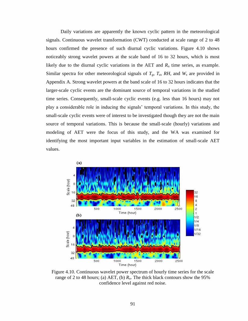
91

Daily variations are apparently the known cyclic pattern in the meteorological

signals. Continuous wavelet transformation (CWT) conducted at scale range of 2 to 48

hours confirmed the presence of such diurnal cyclic variations. Figure 4.10 shows

noticeably strong wavelet powers at the scale band of 16 to 32 hours, which is most

likely due to the diurnal cyclic variations in the AET and Rn time series, as example.

Similar spectra for other meteorological signals of Tg, Ta, RH, and Ws are provided in

Appendix A. Strong wavelet powers at the band scale of 16 to 32 hours indicates that the

larger-scale cyclic events are the dominant source of temporal variations in the studied

time series. Consequently, small-scale cyclic events (e.g. less than 16 hours) may not

play a considerable role in inducing the signals’ temporal variations. In this study, the

small-scale cyclic events were of interest to be investigated though they are not the main

source of temporal variations. This is because the small-scale (hourly) variations and

modeling of AET were the focus of this study, and the WA was examined for

identifying the most important input variables in the estimation of small-scale AET

values.

Figure 4.10. Continuous wavelet power spectrum of hourly time series for the scale

range of 2 to 48 hours; (a) AET, (b) Rn. The thick black contours show the 95%

confidence level against red noise.

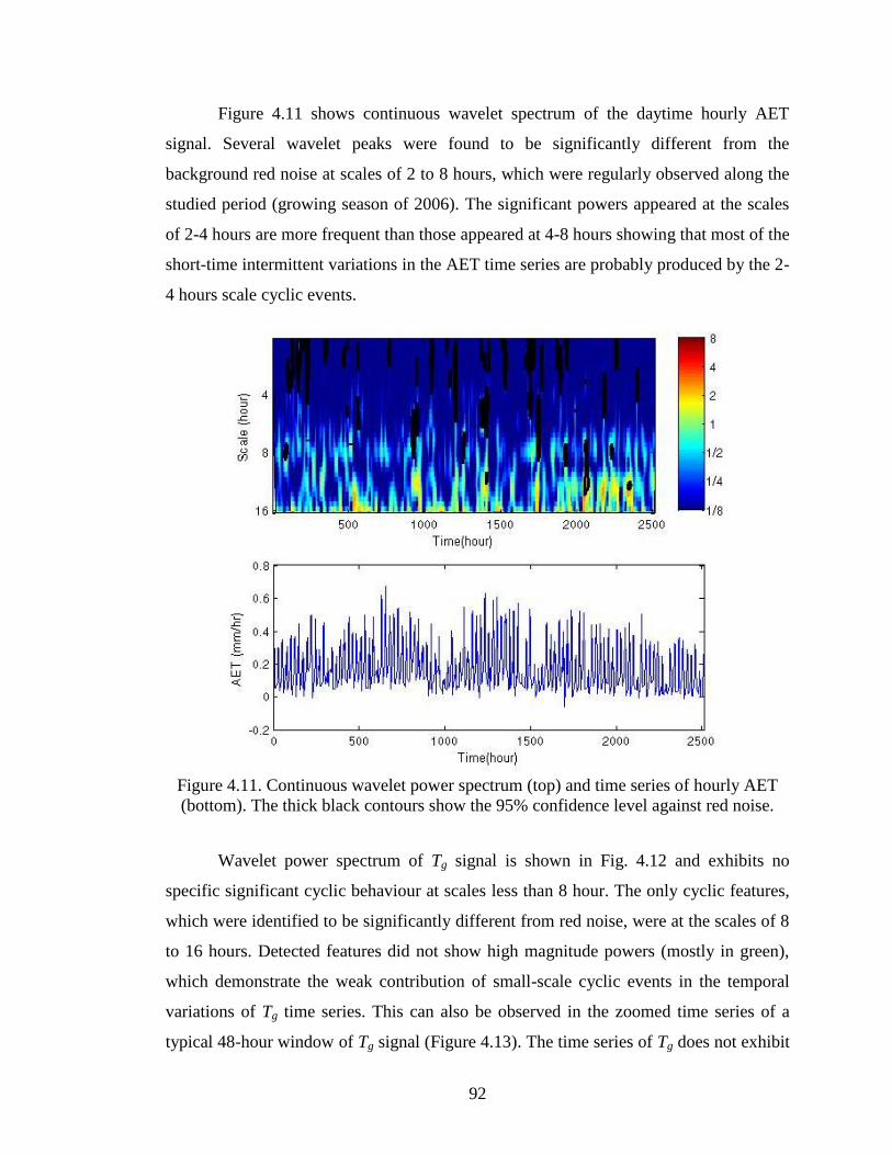
92

Figure 4.11 shows continuous wavelet spectrum of the daytime hourly AET

signal. Several wavelet peaks were found to be significantly different from the

background red noise at scales of 2 to 8 hours, which were regularly observed along the

studied period (growing season of 2006). The significant powers appeared at the scales

of 2-4 hours are more frequent than those appeared at 4-8 hours showing that most of the

short-time intermittent variations in the AET time series are probably produced by the 2-

4 hours scale cyclic events.

Figure 4.11. Continuous wavelet power spectrum (top) and time series of hourly AET

(bottom). The thick black contours show the 95% confidence level against red noise.

Wavelet power spectrum of Tg signal is shown in Fig. 4.12 and exhibits no

specific significant cyclic behaviour at scales less than 8 hour. The only cyclic features,

which were identified to be significantly different from red noise, were at the scales of 8

to 16 hours. Detected features did not show high magnitude powers (mostly in green),

which demonstrate the weak contribution of small-scale cyclic events in the temporal

variations of Tg time series. This can also be observed in the zoomed time series of a

typical 48-hour window of Tg signal (Figure 4.13). The time series of Tg does not exhibit

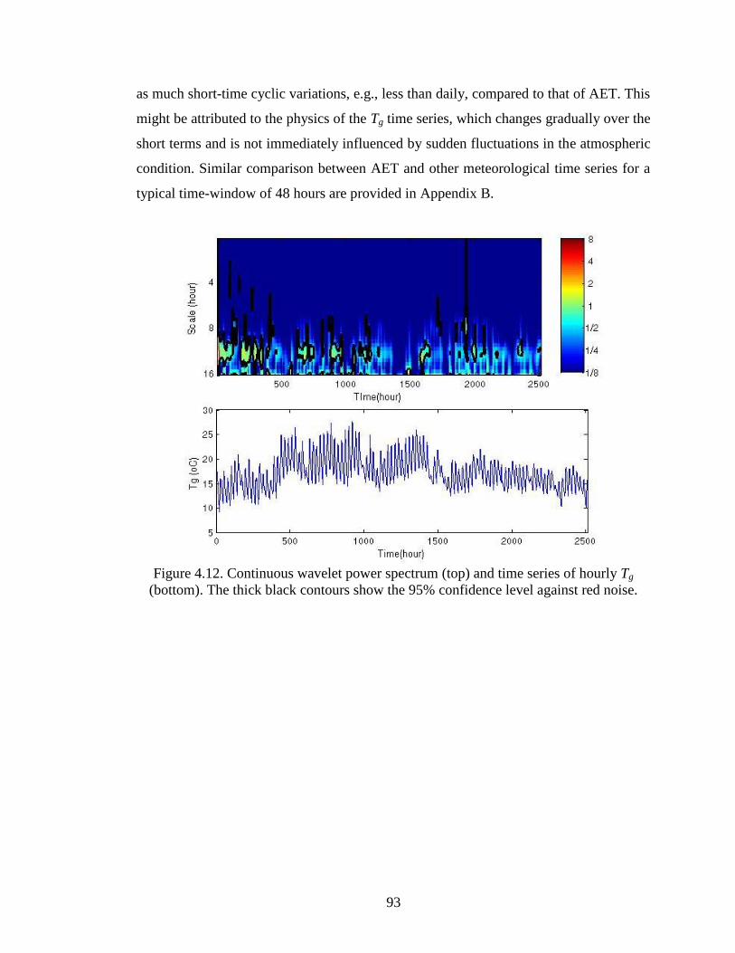
93

as much short-time cyclic variations, e.g., less than daily, compared to that of AET. This

might be attributed to the physics of the Tg time series, which changes gradually over the

short terms and is not immediately influenced by sudden fluctuations in the atmospheric

condition. Similar comparison between AET and other meteorological time series for a

typical time-window of 48 hours are provided in Appendix B.

Figure 4.12. Continuous wavelet power spectrum (top) and time series of hourly Tg


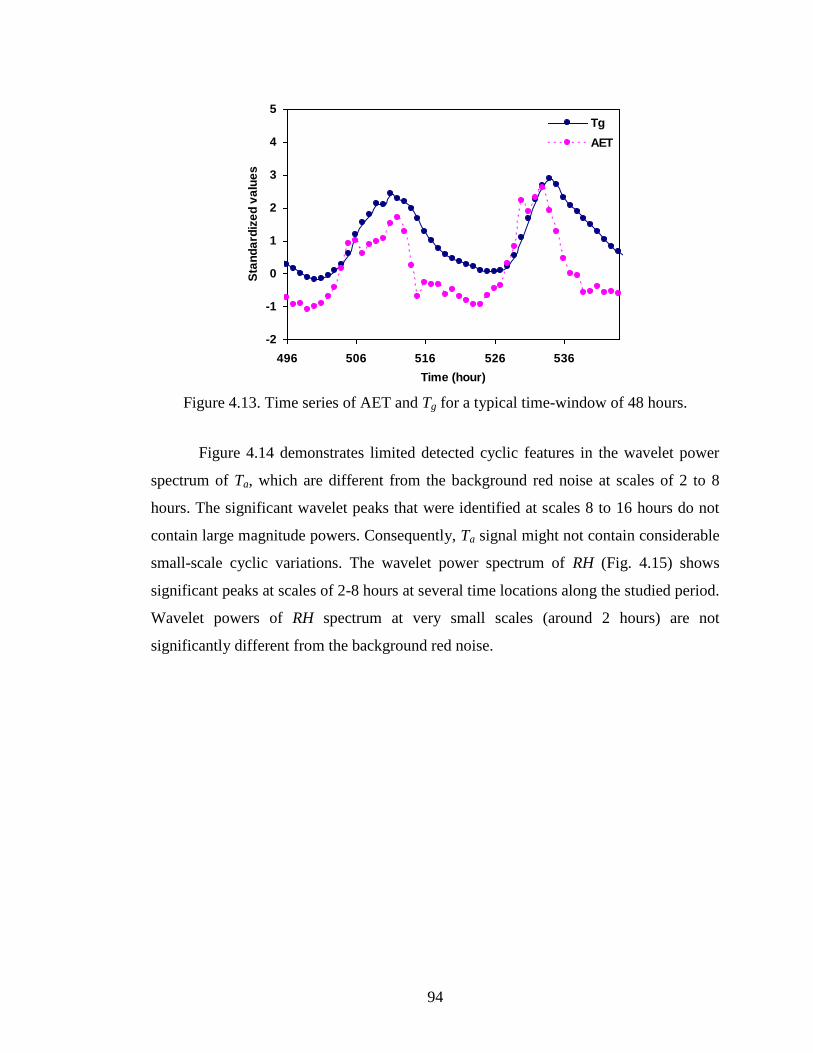
94

Figure 4.13. Time series of AET and Tg for a typical time-window of 48 hours.

Figure 4.14 demonstrates limited detected cyclic features in the wavelet power

spectrum of Ta, which are different from the background red noise at scales of 2 to 8

hours. The significant wavelet peaks that were identified at scales 8 to 16 hours do not

contain large magnitude powers. Consequently, Ta signal might not contain considerable

small-scale cyclic variations. The wavelet power spectrum of RH (Fig. 4.15) shows

significant peaks at scales of 2-8 hours at several time locations along the studied period.

Wavelet powers of RH spectrum at very small scales (around 2 hours) are not

significantly different from the background red noise.

-2

-1

0

1

2

3

4

5

496 506 516 526 536

Time (hour)

Sta

nd

ard

ize

d v

alu

es

Tg

AET

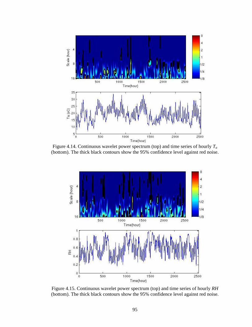
95

Figure 4.14. Continuous wavelet power spectrum (top) and time series of hourly Ta


Figure 4.15. Continuous wavelet power spectrum (top) and time series of hourly RH


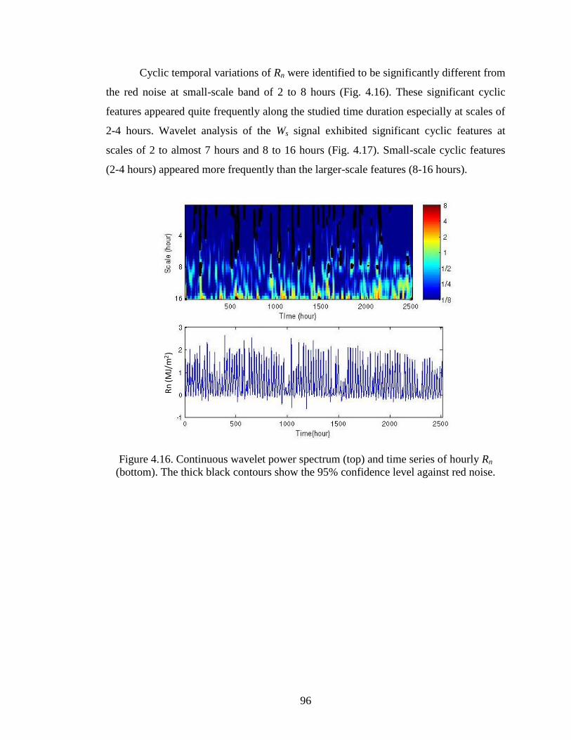
96

Cyclic temporal variations of Rn were identified to be significantly different from

the red noise at small-scale band of 2 to 8 hours (Fig. 4.16). These significant cyclic

features appeared quite frequently along the studied time duration especially at scales of

2-4 hours. Wavelet analysis of the Ws signal exhibited significant cyclic features at

scales of 2 to almost 7 hours and 8 to 16 hours (Fig. 4.17). Small-scale cyclic features

(2-4 hours) appeared more frequently than the larger-scale features (8-16 hours).

Figure 4.16. Continuous wavelet power spectrum (top) and time series of hourly Rn


Rn

(MJ/

m2)

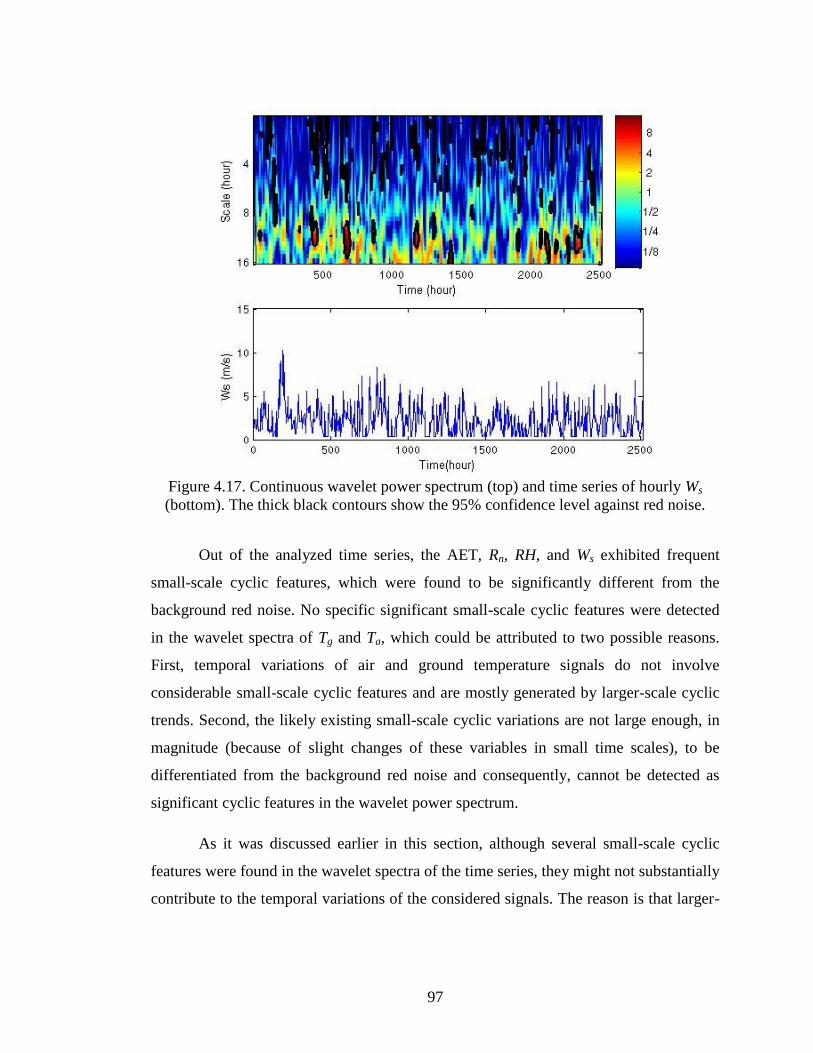
97

Figure 4.17. Continuous wavelet power spectrum (top) and time series of hourly Ws


Out of the analyzed time series, the AET, Rn, RH, and Ws exhibited frequent

small-scale cyclic features, which were found to be significantly different from the

background red noise. No specific significant small-scale cyclic features were detected

in the wavelet spectra of Tg and Ta, which could be attributed to two possible reasons.

First, temporal variations of air and ground temperature signals do not involve

considerable small-scale cyclic features and are mostly generated by larger-scale cyclic

trends. Second, the likely existing small-scale cyclic variations are not large enough, in

magnitude (because of slight changes of these variables in small time scales), to be

differentiated from the background red noise and consequently, cannot be detected as

significant cyclic features in the wavelet power spectrum.

As it was discussed earlier in this section, although several small-scale cyclic

features were found in the wavelet spectra of the time series, they might not substantially

contribute to the temporal variations of the considered signals. The reason is that larger-

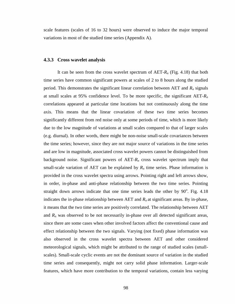
98

scale features (scales of 16 to 32 hours) were observed to induce the major temporal

variations in most of the studied time series (Appendix A).

4.3.3 Cross wavelet analysis

It can be seen from the cross wavelet spectrum of AET-Rn (Fig. 4.18) that both

time series have common significant powers at scales of 2 to 8 hours along the studied

period. This demonstrates the significant linear correlation between AET and Rn signals

at small scales at 95% confidence level. To be more specific, the significant AET-Rn

correlations appeared at particular time locations but not continuously along the time

axis. This means that the linear covariation of these two time series becomes

significantly different from red noise only at some periods of time, which is more likely

due to the low magnitude of variations at small scales compared to that of larger scales

(e.g. diurnal). In other words, there might be non-noise small-scale covariances between

the time series; however, since they are not major source of variations in the time series

and are low in magnitude, associated cross wavelet powers cannot be distinguished from

background noise. Significant powers of AET-Rn cross wavelet spectrum imply that

small-scale variation of AET can be explained by Rn time series. Phase information is

provided in the cross wavelet spectra using arrows. Pointing right and left arrows show,

in order, in-phase and anti-phase relationship between the two time series. Pointing

straight down arrows indicate that one time series leads the other by 90o. Fig. 4.18

indicates the in-phase relationship between AET and Rn at significant areas. By in-phase,

it means that the two time series are positively correlated. The relationship between AET

and Rn was observed to be not necessarily in-phase over all detected significant areas,

since there are some cases when other involved factors affect the conventional cause and

effect relationship between the two signals. Varying (not fixed) phase information was

also observed in the cross wavelet spectra between AET and other considered

meteorological signals, which might be attributed to the range of studied scales (small-

scales). Small-scale cyclic events are not the dominant source of variation in the studied

time series and consequently, might not carry solid phase information. Larger-scale

features, which have more contribution to the temporal variations, contain less varying

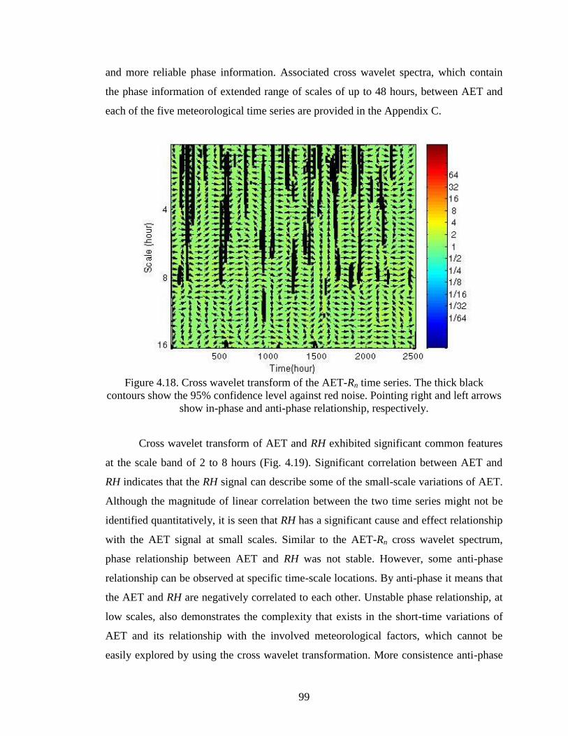
99

and more reliable phase information. Associated cross wavelet spectra, which contain

the phase information of extended range of scales of up to 48 hours, between AET and

each of the five meteorological time series are provided in the Appendix C.

Figure 4.18. Cross wavelet transform of the AET-Rn time series. The thick black


show in-phase and anti-phase relationship, respectively.

Cross wavelet transform of AET and RH exhibited significant common features

at the scale band of 2 to 8 hours (Fig. 4.19). Significant correlation between AET and

RH indicates that the RH signal can describe some of the small-scale variations of AET.

Although the magnitude of linear correlation between the two time series might not be

identified quantitatively, it is seen that RH has a significant cause and effect relationship

with the AET signal at small scales. Similar to the AET-Rn cross wavelet spectrum,

phase relationship between AET and RH was not stable. However, some anti-phase

relationship can be observed at specific time-scale locations. By anti-phase it means that

the AET and RH are negatively correlated to each other. Unstable phase relationship, at

low scales, also demonstrates the complexity that exists in the short-time variations of

AET and its relationship with the involved meteorological factors, which cannot be

easily explored by using the cross wavelet transformation. More consistence anti-phase

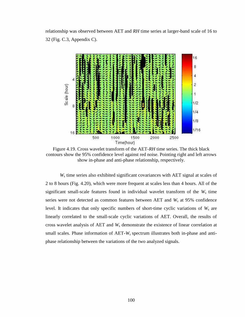
100

relationship was observed between AET and RH time series at larger-band scale of 16 to

32 (Fig. C.3, Appendix C).

Figure 4.19. Cross wavelet transform of the AET-RH time series. The thick black



Ws time series also exhibited significant covariances with AET signal at scales of

2 to 8 hours (Fig. 4.20), which were more frequent at scales less than 4 hours. All of the

significant small-scale features found in individual wavelet transform of the Ws time

series were not detected as common features between AET and Ws at 95% confidence

level. It indicates that only specific numbers of short-time cyclic variations of Ws are

linearly correlated to the small-scale cyclic variations of AET. Overall, the results of

cross wavelet analysis of AET and Ws demonstrate the existence of linear correlation at

small scales. Phase information of AET-Ws spectrum illustrates both in-phase and anti-

phase relationship between the variations of the two analyzed signals.

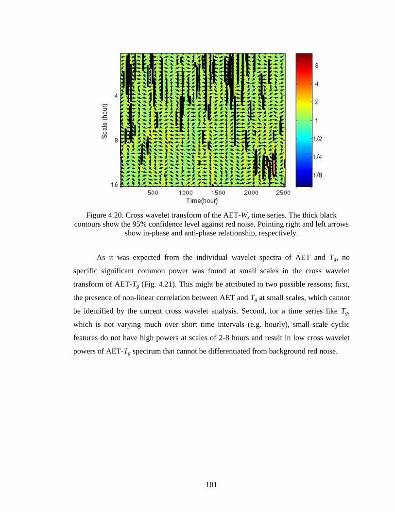
101

Figure 4.20. Cross wavelet transform of the AET-Ws time series. The thick black



As it was expected from the individual wavelet spectra of AET and Tg, no

specific significant common power was found at small scales in the cross wavelet

transform of AET-Tg (Fig. 4.21). This might be attributed to two possible reasons; first,

the presence of non-linear correlation between AET and Tg at small scales, which cannot

be identified by the current cross wavelet analysis. Second, for a time series like Tg,

which is not varying much over short time intervals (e.g. hourly), small-scale cyclic

features do not have high powers at scales of 2-8 hours and result in low cross wavelet

powers of AET-Tg spectrum that cannot be differentiated from background red noise.

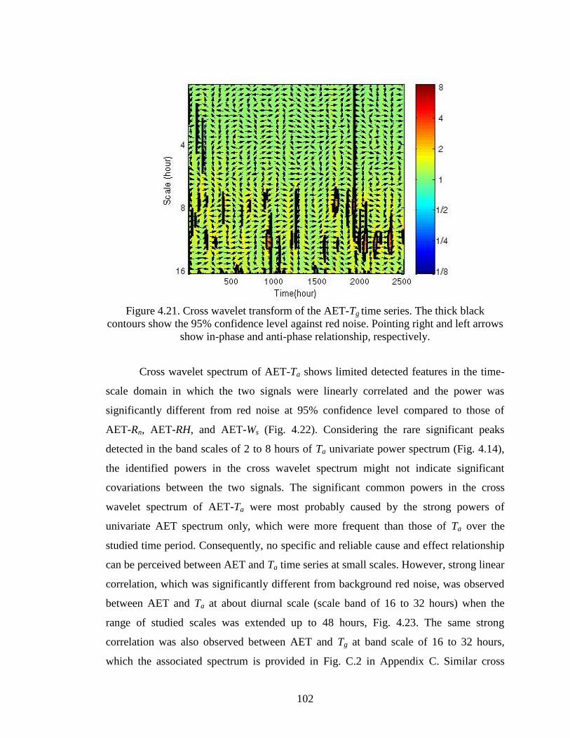
102

Figure 4.21. Cross wavelet transform of the AET-Tg time series. The thick black



Cross wavelet spectrum of AET-Ta shows limited detected features in the time-

scale domain in which the two signals were linearly correlated and the power was

significantly different from red noise at 95% confidence level compared to those of

AET-Rn, AET-RH, and AET-Ws (Fig. 4.22). Considering the rare significant peaks

detected in the band scales of 2 to 8 hours of Ta univariate power spectrum (Fig. 4.14),

the identified powers in the cross wavelet spectrum might not indicate significant

covariations between the two signals. The significant common powers in the cross

wavelet spectrum of AET-Ta were most probably caused by the strong powers of

univariate AET spectrum only, which were more frequent than those of Ta over the

studied time period. Consequently, no specific and reliable cause and effect relationship

can be perceived between AET and Ta time series at small scales. However, strong linear

correlation, which was significantly different from background red noise, was observed

between AET and Ta at about diurnal scale (scale band of 16 to 32 hours) when the

range of studied scales was extended up to 48 hours, Fig. 4.23. The same strong

correlation was also observed between AET and Tg at band scale of 16 to 32 hours,

which the associated spectrum is provided in Fig. C.2 in Appendix C. Similar cross

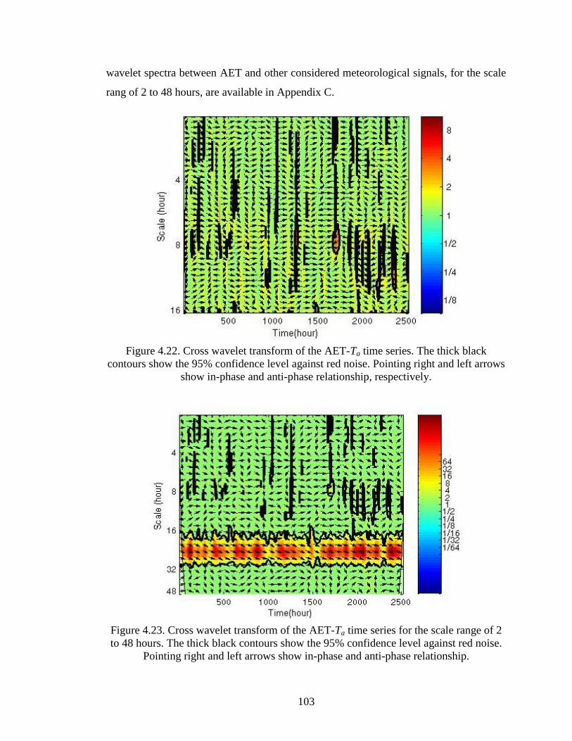
103

wavelet spectra between AET and other considered meteorological signals, for the scale

rang of 2 to 48 hours, are available in Appendix C.

Figure 4.22. Cross wavelet transform of the AET-Ta time series. The thick black



Figure 4.23. Cross wavelet transform of the AET-Ta time series for the scale range of 2

to 48 hours. The thick black contours show the 95% confidence level against red noise.

Pointing right and left arrows show in-phase and anti-phase relationship.

104

The results of the cross wavelet analysis determined, to some extent, the

meteorological variables that have significant linear correlation with the AET signal at

small scales at 95% confidence level. Based on the cross wavelet analysis, Rn, RH, and

Ws time series exhibited significant correlation with the AET signal and therefore, they

are the important variables in the prediction of small-scale AET variations. Based on the

values provided on the scales (color bars) of the cross wavelet spectra, Rn exhibited

stronger correlation with AET than RH, which is stronger than Ws, with maximum cross

wavelet power magnitudes of 256, 16, and 8, respectively. Unfortunately, the results of

the cross wavelet analysis cannot be interpreted in a precise quantitative way to identify

the importance of one variable over others in the prediction of AET at specific scales (or

band scales). In addition, significant powers detected in the univariant wavelet spectra

must always be considered when significant cross wavelet powers are interpreted. This

is to avoid false common powers, which might be created by the large magnitude powers

of one univariate spectrum only.

Based on the cross wavelet analysis, ground temperature has no important linear

correlation with the AET time series at small scales. As a result, one might not select Tg

as a predictor in the estimation of AET. However, the results of the data driven modeling

demonstrated the importance of ground temperature in the prediction of AET. This

inconsistency might be attributed to the previously mentioned ability of cross wavelet

analysis in identifying only linear correlations between time series. As a result, any

existing non-linear correlation between each pair of signals remains undiscovered using

cross wavelet analysis. Another possible reason for insignificant common powers in

AET-Tg cross wavelet spectrum is that the cross wavelet analysis can investigate the

correlation between only two time series at a time (not multiple time series), which

ignores the possible effect of other factors interacting with the considered signals. The

importance of interaction effects, which exist among the variables involved in the AET

process, was observed in the results of the data driven modeling. The above-mentioned

limitations of cross wavelet analysis affect the accuracy of the correlation analysis of

time series for determining the most important AET predictors.

105

The other issue, which most probably resulted in the inconsistency between the

findings of wavelet analysis and data driven modeling is the time-scale at which the

temporal variations of signals were investigated using wavelet analysis or modeled by

data driven techniques. The results of the cross wavelet analysis at the larger-scales

(scale range of 16 to 32 hours, Appendix C) were in agreement with the results of the

data driven models, regarding the most effective variables in the prediction of AET.

Cross wavelet analysis exhibited strong linear correlation between AET and Tg at about

diurnal scale approximately over the whole studied period. As a result, it can be

perceived that the proposed data driven models mainly characterized the larger-scale

variations of AET (the dominant cyclic patterns) for which Rn and Tg were found to be

the most effective predictors. The cross wavelet analysis, conducted in the present study,

concerned more about the small-scale variations of AET. The results obtained using the

WA at small scales might be useful in the development of AET models that aim to

characterize the small-scale temporal variations.

Wind speed is another example of which the time-scale of its variations is of

high importance to be considered in the analysis and may result in some conflict.

Wavelet analysis demonstrated that Ws is one of the important variables in the prediction

of AET at the small-scale bands (e.g. 2-8 hours). However, Ws was rarely identified by

the data driven models, GP and MLR, to be an important variable in the estimation of

AET. Simple visual comparison between AET and Ws time series (Fig. B.2, Appendix

B), and the univariate wavelet spectrum of Ws at larger scales (Fig. A.4, Appendix A)

indicated that larger-scale cyclic features (e.g. diurnal) are not the dominant source of

variations in the Ws time series. Consequently, it is less probable, for Ws, to be identified

as important input variable by the data driven models, which capture mainly the larger-

scale cyclic patterns. The above-mentioned discussion highlights the importance of the

time-scale of temporal variations, which might be of interest to be investigated,

analyzed, and modeled. Depending on the specific time-scale of variations one is

interested in, the employed modeling technique and/or, for instance, the range of studied

scales in the wavelet analysis may vary. As a result, it is important to have better

understanding of different types of temporal variation exist in the investigated time

series prior to the signal analysis and/or modeling.

106

The correlation between AET and a combination of multiple predictor time series

can be investigated by using cross wavelet transform between observed AET and GP

models-predicted AET time series. The results of this specific analysis can highlight the

importance of multiple combined predictors, rather than individual predictors, in

explaining the small-scale cyclic variations of AET. The GP-evolved predictor signals

are composed of different combinations of meteorological variables, which consider the

effect of multiple predictors together (interaction effects). These GP-predicted AET

signals also include the non-linear combinations of inputs by which the importance of

non-linear correlations can also be investigated in the cross wavelet transform.

The four GP models, which were used as combined predictor signals, are given

as follow:

238.0036.009.31.01.0723.0

38.01.002.0

ngSS

nSg

RTRHWW

RWTAET [4.20]

RH

RHWRRHRTTAET S

nngg03.1

103.1097.077.0103.1147.0383.0024.0005.0

[4.21]

aagngn TTTRTRAET 0045.00296.058.000033.0009.02

[4.22]

185.016.0015.0 ng RTAET [4.23]

Cross wavelet transform of observed AET and combined predictors (GP models)

is shown in Fig.4.24. Significant common features were found to be different from red

noise at small-scale band of 2 to 8 hours for all four GP-evolved signals. Identified cross

wavelet powers demonstrate the significant linear correlation between the observed AET

and combined predictor time series (obtained from GP models). Significant cyclic

features in the individual wavelet transform of AET (Fig. 4.11) appeared to be

significant in the cross wavelet spectra of Fig. 4.24, which demonstrates the ability of all

four combined predictor signals in the estimation of small-scale cyclic variations of

AET. In other words, the GP technique, which was found to mainly characterize the

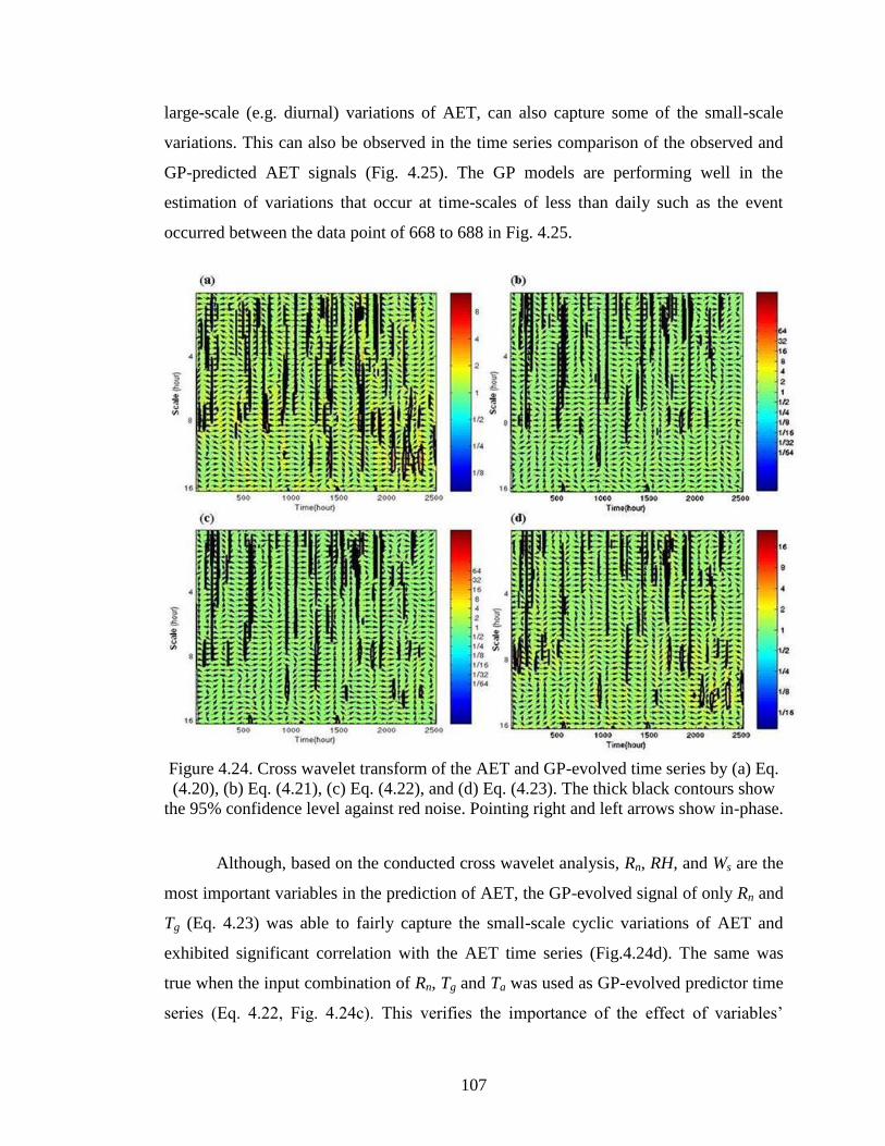
107

large-scale (e.g. diurnal) variations of AET, can also capture some of the small-scale

variations. This can also be observed in the time series comparison of the observed and

GP-predicted AET signals (Fig. 4.25). The GP models are performing well in the

estimation of variations that occur at time-scales of less than daily such as the event

occurred between the data point of 668 to 688 in Fig. 4.25.

Figure 4.24. Cross wavelet transform of the AET and GP-evolved time series by (a) Eq.

(4.20), (b) Eq. (4.21), (c) Eq. (4.22), and (d) Eq. (4.23). The thick black contours show

the 95% confidence level against red noise. Pointing right and left arrows show in-phase.

Although, based on the conducted cross wavelet analysis, Rn, RH, and Ws are the

most important variables in the prediction of AET, the GP-evolved signal of only Rn and

Tg (Eq. 4.23) was able to fairly capture the small-scale cyclic variations of AET and

exhibited significant correlation with the AET time series (Fig.4.24d). The same was

true when the input combination of Rn, Tg and Ta was used as GP-evolved predictor time

series (Eq. 4.22, Fig. 4.24c). This verifies the importance of the effect of variables’

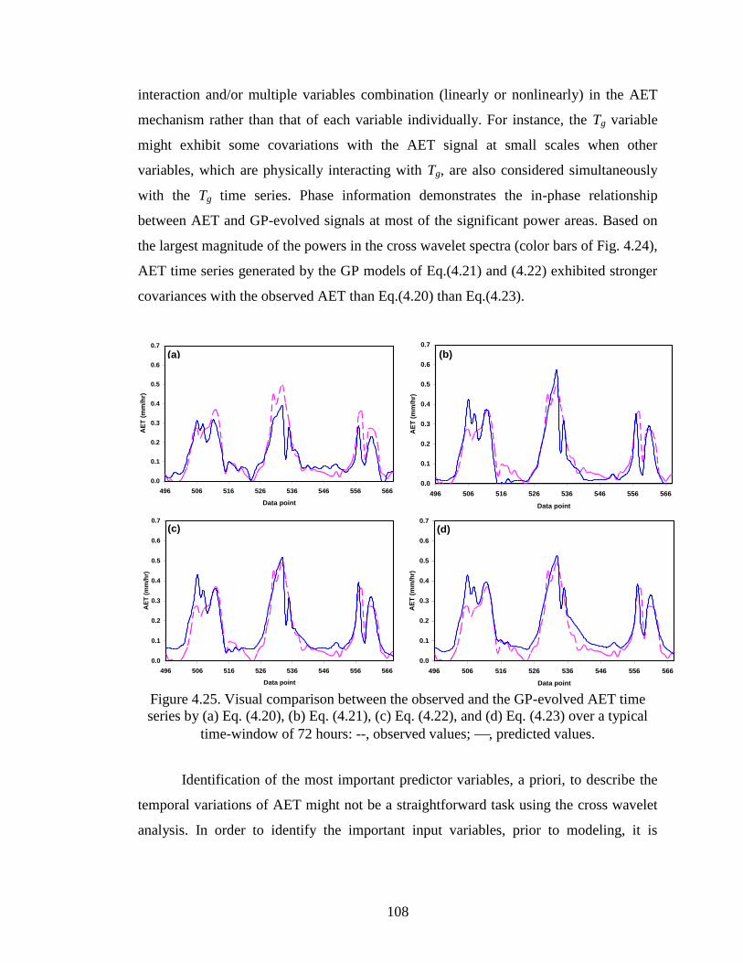
108

interaction and/or multiple variables combination (linearly or nonlinearly) in the AET

mechanism rather than that of each variable individually. For instance, the Tg variable

might exhibit some covariations with the AET signal at small scales when other

variables, which are physically interacting with Tg, are also considered simultaneously

with the Tg time series. Phase information demonstrates the in-phase relationship

between AET and GP-evolved signals at most of the significant power areas. Based on

the largest magnitude of the powers in the cross wavelet spectra (color bars of Fig. 4.24),

AET time series generated by the GP models of Eq.(4.21) and (4.22) exhibited stronger

covariances with the observed AET than Eq.(4.20) than Eq.(4.23).

Figure 4.25. Visual comparison between the observed and the GP-evolved AET time

series by (a) Eq. (4.20), (b) Eq. (4.21), (c) Eq. (4.22), and (d) Eq. (4.23) over a typical

time-window of 72 hours: --, observed values; , predicted values.

Identification of the most important predictor variables, a priori, to describe the

temporal variations of AET might not be a straightforward task using the cross wavelet

analysis. In order to identify the important input variables, prior to modeling, it is

0.0

0.1

0.2

0.3

0.4

0.5

0.6

0.7

496 506 516 526 536 546 556 566

Data point

AE

T (

mm

/hr)

(a)

0.0

0.1

0.2

0.3

0.4

0.5

0.6

0.7

496 506 516 526 536 546 556 566

Data point

AE

T (

mm

/hr)

(b)

0.0

0.1

0.2

0.3

0.4

0.5

0.6

0.7

496 506 516 526 536 546 556 566

Data point

AE

T (

mm

/hr)

(c)

0.0

0.1

0.2

0.3

0.4

0.5

0.6

0.7

496 506 516 526 536 546 556 566

Data point

AE

T (

mm

/hr)

(d)

109

important to consider, in advance, the capabilities/limitations of the wavelet analysis as

well as the complexity of the mechanism under consideration.

4.4 Discussion

Among the proposed models in this study, the GP and MLR models are both

equation-based. Such explicit equation-based models are more appealing to hydrological

practitioners because of the transparency and the simplicity of their application. The

variables that were observed to have the largest contribution to the AET prediction are

almost the same for both equation-based modeling techniques; indicating that both GP

and MLR techniques are able to adequately capture the most suitable meteorological

variables. Based on the GP and MLR models, the meteorological variables, which were

dominantly contributing to the prediction of AET variations (mainly large-scale, e.g.

diurnal), include net radiation (Rn) and ground temperature (Tg). Rn is a known variable,

which is the source of energy and is one of the essential elements in the

evapotranspiration mechanism. The other important elements that shapes the physics of

the evaporation are characterized by the surface soil moisture, surface soil temperature,

and turbulent sensible heat flux (Wang et al., 2004).

Strong land-atmosphere interaction results in dynamic feedbacks among the

involved processes in which the land surface states contain important signal of the near

surface atmospheric condition. Sensible heat flux represents the free and forced

turbulent transport of heat to the atmosphere caused by surface thermal instabilities and

turbulent eddies of wind, respectively. Sensible heat flux as an indication of turbulent

transport in the evaporation mechanism (Obukhov, 1946, cited by Wang et al., 2004) is

physically related to the state variables of soil moisture and soil temperature (Wang et

al., 2004). Wang et al. (2004) also found that the near surface humidity condition can be

captured by the surface variables, such as soil moisture and soil temperature. Soil

moisture is not easily measurable for most case studies, especially when short temporal

scale is required for consistency with the time resolution of other variables. For this

study, the hourly data of soil moisture was not available, and temporal downscaling

110

(disaggregation) of large time-scale soil moisture data to hourly data involves

uncertainty. Although no information on soil moisture level was considered for the

modeling purposes, it was observed that the net radiation and soil temperature variables

(as the dominant inputs in the explicit proposed models) were able to properly

compensate for the absence of soil moisture information and sufficiently estimate the

variation of AET. This can be attributed to the influence of the upper soil layer moisture

on the net radiation, Bowen ratio, and subsequently ground temperature.

Physical description of the AET mechanism, which can be found in many texts

and literature (e.g. Dingman 2002; Wang et al., 2004), properly explains the importance

of soil moisture element and its complex interaction with other land-atmosphere

variables in the AET process. It was of interest to investigate the level of cause and

effect relationship between the variations of AET and soil moisture condition in

comparison with that of AET and meteorological variables, such as Rn and Tg, at small

time-scales. In order to conduct this comparison, the time series of AET, soil water

content, Rn, and Tg were visually compared over a typical time-window. Since only the

six-hourly information of soil moisture was available, the comparison was conducted

using the six-hour time resolution of data. Figure 2.26 shows the temporal variations of

six-hour Rn, Tg, soil water content, and AET data series for a typical time-window of 13

days, which includes the data of daytime only. As it is expected from the physics of soil

moisture time series, the soil water content varies slightly in time compared to Rn, Tg,

and AET variables (Fig.4.26). It can be seen that over the time period of 13 days the soil

water content is decreasing gradually, which results in a reduction in the AET value at

the end of the time period compared to that at the beginning. Consequently, it is difficult

to say if the soil moisture would influence the estimation of AET over shorter-time

periods, e.g. daily or less.

Temporal intermittent variations observed in the data series of AET, Rn, and Tg

(Fig. 4.26) mainly reflect the diurnal scale variations, since only daytime six-hour data

(11:16 AM and 5:16 PM) were considered. Both examined meteorological variables, Rn

and Tg, exhibit strong correlation with AET at this scale, which confirms the results of

the data driven models and the wavelet analysis (at larger-scales) regarding the most

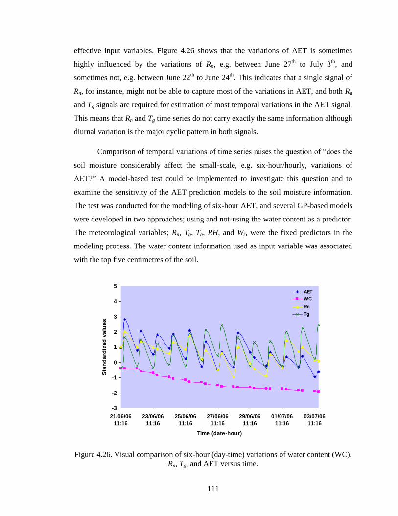
111

effective input variables. Figure 4.26 shows that the variations of AET is sometimes

highly influenced by the variations of Rn, e.g. between June 27th

to July 3th

, and

sometimes not, e.g. between June 22th

to June 24th

. This indicates that a single signal of

Rn, for instance, might not be able to capture most of the variations in AET, and both Rn

and Tg signals are required for estimation of most temporal variations in the AET signal.

This means that Rn and Tg time series do not carry exactly the same information although

diurnal variation is the major cyclic pattern in both signals.

Comparison of temporal variations of time series raises the question of ―does the

soil moisture considerably affect the small-scale, e.g. six-hour/hourly, variations of

AET?‖ A model-based test could be implemented to investigate this question and to

examine the sensitivity of the AET prediction models to the soil moisture information.

The test was conducted for the modeling of six-hour AET, and several GP-based models

were developed in two approaches; using and not-using the water content as a predictor.

The meteorological variables; Rn, Tg, Ta, RH, and Ws, were the fixed predictors in the

modeling process. The water content information used as input variable was associated

with the top five centimetres of the soil.

Figure 4.26. Visual comparison of six-hour (day-time) variations of water content (WC),

Rn, Tg, and AET versus time.

-3

-2

-1

0

1

2

3

4

5

21/06/06

11:16

23/06/06

11:16

25/06/06

11:16

27/06/06

11:16

29/06/06

11:16

01/07/06

11:16

03/07/06

11:16

Time (date-hour)

Sta

nd

ard

ize

d v

alu

es

AET

WC

Rn

Tg

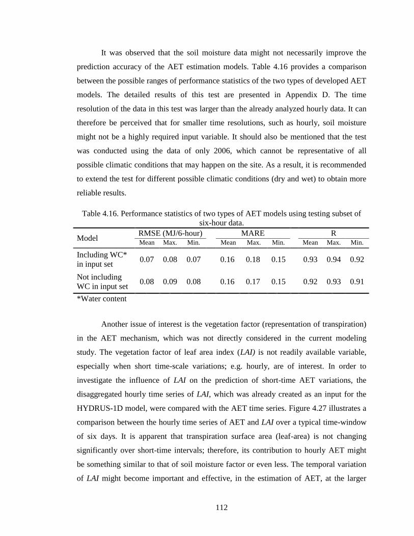
112

It was observed that the soil moisture data might not necessarily improve the

prediction accuracy of the AET estimation models. Table 4.16 provides a comparison

between the possible ranges of performance statistics of the two types of developed AET

models. The detailed results of this test are presented in Appendix D. The time

resolution of the data in this test was larger than the already analyzed hourly data. It can

therefore be perceived that for smaller time resolutions, such as hourly, soil moisture

might not be a highly required input variable. It should also be mentioned that the test

was conducted using the data of only 2006, which cannot be representative of all

possible climatic conditions that may happen on the site. As a result, it is recommended

to extend the test for different possible climatic conditions (dry and wet) to obtain more

reliable results.

Table 4.16. Performance statistics of two types of AET models using testing subset of

six-hour data.

Model RMSE (MJ/6-hour) MARE R Mean Max. Min. Mean Max. Min. Mean Max. Min.

Including WC*

in input set 0.07 0.08 0.07 0.16 0.18 0.15 0.93 0.94 0.92

Not including

WC in input set 0.08 0.09 0.08 0.16 0.17 0.15 0.92 0.93 0.91

*Water content

Another issue of interest is the vegetation factor (representation of transpiration)

in the AET mechanism, which was not directly considered in the current modeling

study. The vegetation factor of leaf area index (LAI) is not readily available variable,

especially when short time-scale variations; e.g. hourly, are of interest. In order to

investigate the influence of LAI on the prediction of short-time AET variations, the

disaggregated hourly time series of LAI, which was already created as an input for the

HYDRUS-1D model, were compared with the AET time series. Figure 4.27 illustrates a

comparison between the hourly time series of AET and LAI over a typical time-window

of six days. It is apparent that transpiration surface area (leaf-area) is not changing

significantly over short-time intervals; therefore, its contribution to hourly AET might

be something similar to that of soil moisture factor or even less. The temporal variation

of LAI might become important and effective, in the estimation of AET, at the larger

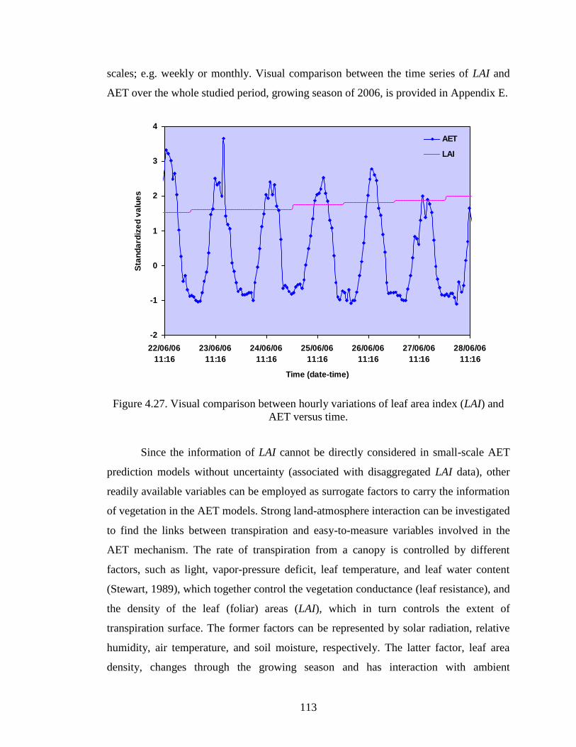
113

scales; e.g. weekly or monthly. Visual comparison between the time series of LAI and

AET over the whole studied period, growing season of 2006, is provided in Appendix E.

Figure 4.27. Visual comparison between hourly variations of leaf area index (LAI) and

AET versus time.

Since the information of LAI cannot be directly considered in small-scale AET

prediction models without uncertainty (associated with disaggregated LAI data), other

readily available variables can be employed as surrogate factors to carry the information

of vegetation in the AET models. Strong land-atmosphere interaction can be investigated

to find the links between transpiration and easy-to-measure variables involved in the

AET mechanism. The rate of transpiration from a canopy is controlled by different

factors, such as light, vapor-pressure deficit, leaf temperature, and leaf water content

(Stewart, 1989), which together control the vegetation conductance (leaf resistance), and

the density of the leaf (foliar) areas (LAI), which in turn controls the extent of

transpiration surface. The former factors can be represented by solar radiation, relative

humidity, air temperature, and soil moisture, respectively. The latter factor, leaf area

density, changes through the growing season and has interaction with ambient

-2

-1

0

1

2

3

4

22/06/06

11:16

23/06/06

11:16

24/06/06

11:16

25/06/06

11:16

26/06/06

11:16

27/06/06

11:16

28/06/06

11:16

Time (date-time)

Sta

nd

ard

ize

d v

alu

es

AET

LAI

114

hydrometeorological functions, such as the effect of transpiration area on the

meteorological variables; e.g. relative humidity and ground temperature. Leaf area

increases through the growing season and shelters the underlying ground area from the

sun, which affects the variable of ground temperature. The study conducted by Sanchez-

Carrillo et al. (2001) demonstrated that more than 75% of the hourly variance of

transpiration (in their case study) can be explained by solar radiation and the residues

can be explained by relative humidity and air temperature.

The not fully understood process of actual evapotranspiration makes it very

difficult to mechanistically capture the interactions existed among the state variables to

present a mathematical relationship between AET and highly correlated meteorological

variables. Explicit data driven models (e.g. GP and MLR) exhibited their capability in

efficiently capturing the variations of AET, and inducing symbolic estimation models,

which are mostly dominated by net radiation and ground temperature. The equation-

based GP technique, which was presented in this study, is not the only capacity of the

GP as an evolutionary data driven technique. GP can also be implemented to evolve

program-based models, which can be presented in a code format, but not as explicit

mathematical expressions (Elshorbagy and El-Baroudy, 2009). The program-based type

of GP has the advantage of using conditional, comparison, and logical operators in

addition to the arithmetic operators, which may enhance the predictive capability of the

model to capture more aspects of the investigated process. This means that the utility of

GP technique can also be examined using a different implementation tool (e.g.,

DiscipulusTM

) to investigate any further improvement in the prediction accuracy.

The cross wavelet analysis may not be essentially strong in determining the

optimum input variables for modeling the small-scale AET variations a priori. However,

it has the potential to provide deep insight for studying the larger scale variations of

AET, e.g. diurnal. Among the examined techniques, GP exhibited to be more efficient

than others in identifying the most relevant meteorological predictors. It should also be

considered that there is no single data driven technique that could capture all complex

processes at all times (Elshorbagy and El-Baroudy, 2009). Consequently, different

115

techniques might be capable of efficiently predicting different challenging components

of the hydrological processes.

116

CHAPTER 5. SUMMARY AND CONCLUSION

This chapter summarizes the work described in this thesis, which includes the

data driven models for the prediction of actual evapotranspiration (AET), and wavelet

analysis for investigating the intermittent variations in the AET and meteorological time

series. Conclusions of the results and analysis, the contribution of the conducted

research, possible future research, and limitations of the study are also provided in this

chapter.

5.1 Summary of the study

The research presented in this thesis focused on the modeling and analysis of

hourly actual evapotranspiration (AET) in a reconstructed landscape, located in northern

Alberta, Canada. The study was conducted in two main parts; data driven modeling of

AET and multiresolution analysis of AET and meteorological time series. Hourly eddy

covariance (EC)-measured AET data were investigated as the target function, whereas

the meteorological variables of net radiation, ground temperature, air temperature,

relative humidity, and wind speed were examined as possible predictors.

In the first part of the study, AET prediction models were developed using three

different data driven techniques; artificial neural networks (ANNs), genetic

programming (GP), and multilinear regression (MLR). The performances of the

developed AET models were evaluated and a comparative analysis was conducted, with

regard to the predictive and generalization abilities of the models, to identify the

possible superiority of one modeling approach over the others. In addition, the result of

the data driven models were compared with those of HYDRUS-1D; a physically-based

model, as a possible alternative to the proposed data driven models for the estimation of

AET.

In the second part of the study, the capability of the wavelet analysis was

examined for possible identification of the most important variables in the modeling of

AET, a priori. This was implemented by performing the continuous wavelet

117

transformation for multiresolution analysis of the temporal variations of the various

signals, and for exploring the dominant frequency events. Then, cross wavelet analysis

was performed between the AET time series and each of the meteorological signals, in

order to find any significant covariances, which show the strong cause and effect

relationship between them.

5.1.1 Data driven modeling

The ANN model with eight hidden neurons trained by Bayesian-regularization

algorithm was found to be the best ANN model, with reasonable generalization ability.

The optimum models generated by GP were linear and non-linear equations predicting

AET as a function of net radiation, ground temperature, air temperature, and relative

humidity. Although some of the GP-evolved models were nonlinear and contained

interactions and/or second orders of variables, the models were all linear in parameters.

Thus, it can be said that GP was able to model the complex process of AET as semi-

linear functions of meteorological variables, which also had good predictive abilities.

Almost half of the optimum GP models estimated AET only as a function of net

radiation and ground temperature. The statistical analysis also revealed that net radiation

and ground temperature were the most dominant climatic variables for predicting actual

evapotranspiration. Furthermore, interaction effects of some meteorological variables

were shown to be important in the modeling of AET. The contribution of the interaction

effects in the estimation models was sometimes even more than those of the individual

variables.

A comparative analysis of the models’ predictive abilities indicated that the GP

and MLR models have better generalization ability than the ANN models for estimating

the hourly actual evapotranspiration as a function of meteorological variables in the case

study presented in this thesis. In comparison with the data driven models, the HYDRUS-

1D model performed on par to other models in one year of data (2005) but poorer in

another year (2006) for the estimation of AET. This indicated that a physically-based

model, such as HYDRUS-1D, might be inferior to the data driven models in terms of the

118

overall prediction accuracy. Compared to the ANNs, the important advantage of the GP

and MLR models is the representation of the explicit equations, which can be easily

interpreted. In addition, GP and MLR models are simpler in the application and usage

than the ANN model. The GP-evolved models required fewer input variables than the

MLR. The interesting point is that the performances of the GP and regression models are

close to each other, although the numbers and combinations of the employed inputs are

quite different for each model.

5.1.2 Wavelet analysis

In this study, wavelet analysis was mainly focused on the small-scale temporal

variations of time series, since variations of AET at small time-scale (hourly) was of

interest to be investigated and modeled. Wavelet analysis was also extended to larger-

scales to have a brief overview of other possible cyclic variations exist in the time series.

Continuous wavelet transformation was performed for the hourly time series of the AET

and the five meteorological variables of Rn, Tg, Ta, RH, and Ws. The continuous wavelet

spectra of AET, Rn, RH, and Ws exhibited significant powers at small scales (e.g. 2-8

hours); however, no specific cyclic features were detected in those of Tg and Ta.

Extension of the range of scales to larger values demonstrated the presence of strong

cyclic features at around diurnal scale in most of the studied time series, including Tg

and Ta. It was observed that the contribution of larger-scale cyclic features to the total

time series variations is considerably higher than those of small scales. In other words,

larger-scale (e.g. diurnal) cyclic patterns can be perceived as the major source of

temporal variations in the AET and most of the meteorological time series.

Cross wavelet analysis between AET and each of the meteorological time series

over the range of small scales demonstrated significant linear covariations between AET

and Rn, RH, and Ws time series. This implies that these meteorological variables are

important in explaining the small-scale variations of AET. As it was expected from the

univariate spectrum of Tg and Ta, cross wavelet spectra of AET-Tg and AET-Ta, did not

exhibit any specific covariations at small scales. However, when the cross wavelet

119

analysis was extended to larger range of scales, stronger covariances were observed

between AET and Rn, RH, Tg, and Ta time series, which were significant at the band

scale of 16 to 32 hours (more likely due to diurnal variations). This indicates that the

variables of Tg and Ta are important predictors for the estimation of larger-scale

variations of AET. Consequently, prior-to-modeling identification of the most important

input variables for the estimation of AET depends on the time-scale of variations, which

is of interest to be modeled. It can subsequently be perceived that the GP and MLR

models, which presented the Tg variable as one of the important inputs, may mainly

capture the larger-scale variations of AET. The wavelet analysis, conducted in this

study, revealed the importance of time-scale issue in the analysis and modeling of

temporal variations exist it the AET and meteorological time series.

5.2 Conclusion

In conclusion, the investigated data driven modeling techniques were promising

for the estimation of the hourly AET mechanism using the observed data, without

assuming or applying significant knowledge of the physics of the process. The choice of

the testing dataset was found to be important for realistically assessing the generalization

ability of the proposed data driven models and also for the determination of the possible

superiority of any of the modeling techniques over others. Among the examined data

driven modeling techniques, genetic programming (GP) and MLR were found to

perform similarly and better than the ANN model with regard to generalization ability.

The GP-evolved models also had the advantage of being structurally simple and

requiring fewer input variables, which is of interest for many hydrological practitioners.

Furthermore, the proposed equation-based models, using GP and MLR, showed

that the AET process has the potential to be estimated by structurally simple (e.g. semi-

linear) models. Equation-based AET models made it possible to extract some

information about the physics of the process. It was observed that the meteorological

variables of Rn and Tg have larger contribution, than other variables, to the estimation of

120

AET. In addition, the interaction effects of the meteorological variables were found to be

important and effective in the estimation of AET.

The results of wavelet analysis improved the understanding of the AET

mechanism by revealing the importance and contributions of different time-scale cyclic

variations exist in the AET time series. This highlights the issue of time-scale and the

importance of its consideration in the modeling and prior-to-modeling input selection

procedure. Although several small-scale cyclic features were detected in the AET signal,

larger-scale variations were found to be the major frequency events at which the

predictant-predictor (AET-meteorological variables) correlation analysis was more clear

and reliable. GP and MLR models were noted to mainly model the larger-scale

(dominant) temporal variations of AET, although short time-scale (hourly) data were

employed for training and developing the models.

Consistency between the results of data driven modeling (especially GP) and

wavelet analysis, regarding the most important predictor variables, at large time-scales

(e.g. diurnal) indicated that wavelet analysis can be employed as a guide for identifying

the most linearly correlated predictors for the modeling of AET. However, limitations of

such signal analysis tool should be considered when it is used for input determination

prior to modeling. Wavelet analysis helped to perceive the difference between the

predictive abilities of various models from a new perspective, which is the time-scale of

variations that the models characterize. For instance, when the performances of two

prediction models are compared, it should be noted if both models are capturing the

same time-scale of variations. Consideration of this point can make the models’

comparative analysis more accurate and fair.

5.3 Contribution of the research

In this study, actual evapotranspiration as one of the major components of the

hydrological cycle was modeled using data driven modeling techniques in a

reconstructed watershed. Determination of the most suitable and efficient prediction

model is important for accurate assessment of AET in a reconstructed watershed in

121

which understanding of the various hydrological processes is essential for improvement

and development of sustainable reclamation strategies.

The proposed AET data driven models can be used for practical estimation of the

AET in the studied reconstructed site using the conventional meteorological variables.

Using the developed equation-based GP models, the hourly values of AET can be

estimated using a few and readily available numbers of meteorological variables, which

are usually measured, or can be measured, in most weather stations. Although the

proposed models were basically developed for the estimation of hourly AET, the AET

values associated with larger time scales can also be obtained by aggregating the hourly

AET values. The AET models represented in this study were local models, which might

be applicable for AET estimations in similar case studies. However, it should be first

verified if the climatic conditions and the general characteristics of the considered sites

are similar to that of the site used for model development. Further studies can be

conducted on assessing the performance of the locally proposed models on other

reconstructed sites. In the case of availability of measured AET and meteorological

variables, data driven techniques can be easily used for developing local AET models.

This kind of modeling could be more efficient and easier than the physically-based and

empirical modeling approaches, which require large number of measured inputs and

estimation of models parameters.

Although data driven models do not require any knowledge about the underlying

process, better understanding of the investigated function and identification of the most

important predictor variables, prior to the modeling, can improve the efficiency and the

predictive ability of the model. The results of this study demonstrated that wavelet

analysis can be used as a tool for this purpose. This study also revealed the importance

of the time-scale of variations, under consideration, in the analysis and modeling of

hydrological time series. This finding could improve the current understanding of the

AET variations as well as its correlation with the predictor variables, which can be very

helpful in the interpretation of prediction models. Temporal variations of a hydrological

time series might occur at different time-scales, and different prediction models might be

suitable for capturing each of them. In addition, the cause and effect relationship

122

between hydrological predictant and predictors may vary when the investigated time-

scale of variation is changed. This kind of information can be employed for the analysis

and modeling of any hydrological time series, which enhances the success of the

modeling procedures and consequently, improves the understanding and monitoring of

the reconstructed watershed hydrology.

5.4 Future work

Some of the possible extensions to the current research study, associated with the

inductive modeling of hydrological processes in the reconstructed watersheds, are as

follows:

Extending the GP modeling of AET and wavelet analysis of time series at

different time-scales (e.g. daily or larger) would help to have better

understanding of the GP models’ prediction abilities at different time-scales and

the applicability of wavelet analysis for prior-to-modeling determination of AET

model inputs;

Performing cross wavelet analysis between each pair of the meteorological

variables can help to identify the input variables, which have inter-dependency

and carry the same information to the model, and clean the final set of important

input variables from redundant variables. This may help in redundancy handling

and determining the most efficient and parsimonious set of model’s important

input;

Studying the influence of soil moisture on the AET prediction models can be

extended to include dry and wet years. Also, the soil moisture content data of the

root zone of the soil layer should be included. This helps to investigate the effect

of soil moisture on AET in dry conditions when required water mostly provided

from lower layers of the soil; and

123

Continuous and cross wavelet analysis can be employed for comparing the

performances of different models in terms of their abilities in capturing different

time-scales variations.

5.5 Study limitations

Some of the limitations and assumptions involved with this study are as follows:

For the modeling and analysis of AET mechanism, only two years of data were

available and used in this study, which might not be sufficient for accurate

modeling and model assessment. Two years of data may not include all extreme

conditions;

The functional set selected for performing the GP algorithm was limited to

simple arithmetic functions. Several different functional operators can be used

for developing the equation-based GP models.

For investigating soil moisture effect on the prediction of six-hour AET, the

water content information of only top five centimetres of the soil was considered;

In the HYDRUS model, crop coefficient was assumed to be one, which means

that the vegetation was assumed to have similar aerodynamic and surface

characteristics as reference surface in the PM equation. This assumption was

made because the mentioned information was not available for the vegetation

cover in the studied site; and

For the statistical analysis, time series data were assumed to have normal

distribution.

124

REFERENCES

Abrahart, R.J. and White, S. 2001. Modelling Sediment Transfer in Malawi: Comparing

Backpropagation Neural Network Solutions Against a Multiple Linear Regression

Benchmark Using Small Data Sets. Phys. Chem. Earth (B) 26(1): 19–24.

Akaike, H. 1974. A new look at statistical model identification. IEEE Trans. Automat.

Contr., AC, 19: 716-722.

Allen, M.R. and Smith, L.A. 1996. Monte Carlo SSA: Detecting irregular oscillations in

the presence of coloured noise, J. Clim., 9: 3373–3404.

Allen, R.G., Pereira, L.S., Raes, D., and Smith M. 1998. Crop evapotranspiration:

guidelines for computing crop water requirements. Irrig. and Drain. Paper No. 56.

Rome: FAO.

Anctil, F. and Coulibaly, P. 2004. Wavelet analysis of the interannual variability in

Southern Quebec streamflow. Journal of Climate 17 (1): 163–173.

Anctil, F. and Tape, D.G. 2004. An exploration of artificial neural network rainfall-

runoff forecasting combined with wavelet decomposition. J. Environ. Eng. Sci., 3:

S121–S128.

ASCE. 2000a. Artificial Neural Networks in Hydrology. I. Preliminary Concepts. J.

Hydrol. Eng., 5(2): 115–123.

ASCE. 2000b. Artificial Neural Networks in Hydrology. II. Hydrologic Applications. J.

Hydrol. Eng., 5(2): 124–137.

ASCE Environmental and Water Resources Institute (ASCE-EWRI). 2004._The ASCE

standardized reference evapotranspiration equation. Standardization of Reference

Evapotranspiration Task Committee Final Rep., Reston, Va.

Aytek, A. and Kisi, O. 2008. A genetic programming approach to suspended sediment

modeling. Journal of Hydrology, 351: 288–298.

Aziz, A.R.A. and Wong, K.F.V. 1992. Neural network approach to the determination of

aquifer parameters. Ground Water, 30(2): 164– 166.

Babovic, V. 2000. Data mining and knowledge discovery in sediment transport.

Comput.-Aided Civ. Infrastruct. Eng., 15(5): 383–389.

Babovic, V. and Keijzer, M. 2002. Declarative and preferential bias in GP-based

scientific discovery. Genet. Program. Evol. Mach., 3(1): 41-79.

Back, T., Hammel, U., and Schwefel, H.P. 1997. Evolutionary Computation: Comments

on the History and Current State. IEEE Transactions on Evolutionary Computation,

1(1): 3-16.

Baldocchi, D.D. 2003. Assessing the eddy covariance technique for evaluating carbon

dioxide exchange rates of ecosystems: Past, present and future. Global Change

Biology, 9: 479−492.

125

Baldocchi, D.D., Hicks, B.B., and Meyers, T.P. 1988. Measuring biosphere–atmosphere

exchanges of biologically related gases with micrometeorological methods.

Ecology, 69: 1331−1340.

Baliunas, S., Frick, P., Sokoloff, D., and Soon, W. 1997. Time scales and trends in the

Central England temperature data (1659– 1990) – a wavelet analysis. Geophysical

Research Letters, 24: 1351–1354.

Banzhaf, W., Nordin, P., Keller, R.E., and France, F. 1998. Genetic Programming: An

Introduction. Morgan Kaufmann Publishers, Inc. San Francisco, California, USA.

Baptist, M.J., Babovic, V., Uthurburu, J.R, Keijzer, M., Uittenbogaard, R.E., Mynett, A.,

and Verwey, A. 2007. On inducing equations for vegetation resistance. Journal of

Hydraulic Research, 45(4): 435–450.

Bernatowicz, S., Leszczynski, S., and Tyczynska, S. 1976. The influence of transpiration

by emergent plants on the water balance in lakes. Aquat. Bot., 2: 275-288.

Bhakar, S.R, Oiha, S., Singh, R.V., and Ansari, A. 2006. Estimation of

evapotranspiration for wheat crop using artificial neural network, Proceedigs, 4th

World Congress on Computers in Agriculture, Orlando, FL, US.

Bhattacharya, B., Price, R.K., and Solomatine, D.P. 2005. Data-driven modelling in the

context of sediment transport. Phys. Chem. Earth, 30(4–5): 297–302.

Birikundavy, S., Labib, R., Trung, H.T., and Rousselle, J. 2002. Performance of Neural

Networks in Daily Streamflow Forecasting. J. Hydrol. Eng., 7(5): 392–398.

Blaney, H.F. and Criddle, W.D. 1950. Determining water requirements in irrigated area

from climatological irrigation data. Soil Conservation Service Technical Paper no.

96. US Department of Agriculture, Washington DC, USA.

Boese, C. 2003. The design and installation of a field instrumentation program for the

evaluation of soil-atmosphere water fluxes in a vegetated cover over saline/sodic

shale overburden. M.Sc. Thesis, University of Saskatchewan, Saskatoon, SK,

Canada.

Box, G.E.P. 1957. Evolutionary operation: A method for increasing industrial

productivity. Appl. Statistics, 6(2): 81–101.

Bremermann, H.J. 1962. Optimization Through Evolution and Recombination, In M.C.

Yovits et al, Editors, Self-Organizing Systems, Spartan Books, Washington, DC:

93-106.

Brunsell, N.A., Ham, J.M., and Owensby, C.E. 2008. Assessing the multi-resolution

information content of remotely sensed variables and elevation for

evapotranspiration in a tall-grass prairie environment. Remote Sens. Environ.,

112(6): 2977-2987.

Brutsaert, W.H. 1982. Evaporation into the Atmosphere. D. Reidel, Dordrecht, The

Netherlands.

Cahill, A.T. 2002. Determination of changes in streamflow variance by means of a

wavelet-based test. Water Resour. Res., 38(6): 1065-1078.

126

Campolo, M., Andreussi, P., and Sodalt, A. 1999. River stage forecasting with a neural

network model. Wat. Res. Res., 35(4): 1191–1197.

Campolo, M., Soldati, A., and Andreussi, P. 2003. Artificial neural network approach to

flood forecasting in the River Arno. Hydrol. Sci. J., 48(3): 381–398.

Carey, S.K. 2008. Growing season energy and water exchange from an oil sands

Overburden reclamation soil cover, Fort McMurray, Alberta, Canada. Hydrol.

Process, 22: 2847–2857.

Chauhan, S. and Shrivastava, R.K. 2009. Performance Evaluation of Reference

Evapotranspiration Estimation Using Climate Based Methods and Artificial Neural

Networks. Water Resource Management, 23(5): 825-837.

Chaikowsky, C.L.A. 2003. Soil moisture regime and salinity on a tailing sand storage

facility. M.Sc. Thesis, University of Alberta, Edmonton, Alberta, Canada.

Chen, X. and Liu, D. 2008. Wavelet analysis on inter-annual variation of precipitation in

Guangdong, China. IAHS publication, 319: 3-9.

Cheng, B. and Titterington, D.M. 1994. Neural networks: A review from a statistical

perspective. Statistical Science, 9(1): 2–54.

Compagnucci, R.H., Blanco, S.A., Figliola, M.A., and Jacovkis, P.M. 2000. Variability

in subtropical Andean Argentinean Atuel river: a wavelet approach. Environmetrics,

11: 251–269.

Coulibaly, P. 2004. Downscaling daily extreme temperatures with genetic programming.

Geophysical Research Letters, 31, L16203, doi:10.1029/2004GL020075.

Coulibaly, P. 2006. Spatial and temporal variability of Canadian seasonal precipitation

(1900-2000). Advances in Water Resources, 29: 1846–1865.

Coulibaly, P. and Burn, D.H. 2004. Wavelet analysis of variability in annual Canadian

streamflows. Water Resource Research 40, W03105, doi:10.1029/2003WR002667.

Cousin, N. and Savic, D.A. 1997. A rainfall-runoff model using genetic programming.

Centre for Systems and Control Engineering; Report No. 97/03, School of

Engineering, University of Exeter, Exeter, United Kingdom.

Cybenko, G. 1989. Approximation by superposition of a sigmoidal function. Math.

Control Signals Syst. 2: 303–314.

Dai, X., Shi, H., Li, Y., Ouyang, Z., and Huo Z. 2009. Artificial neural network models

for estimating regional reference evapotranspiration based on climate factors.

Hydrological processes, 23(3): 442-450.

Daniel, T.M. 1991. Neural networks—applications in hydrology and water resources

engineering. Proceedings, Int. Hydrol. and Water Resour. Symp., Institution of

Engineers, Perth, Australia.

Dartus, D., Courivaud, J.M., and Dedecker, L. 1993. Use of a neural net for the study of

a flood wave propagation in an open channel. J. Hydr. Res., 31(2): 161-169.

Daubechies. I. 1988. Orthonormal Bases of Compactly Supported Wavelets. Comm.

Pure Appl. Math., 41: 906-966.

127

Daubechies, I. 1992. Ten Lectures on Wavelets. Society for Industrial and Applied

Mathematics, 357 pp.

Davis, L. (Ed.) 1991. Handbook of Genetic Algorithms. Van Nostrand Reinhold, N.Y.

Dawson, C.W. and Wilby, R.L. 2001. Hydrological modelling using artificial neural

networks. Progress in Physical Geography 25(1): 80–108.

De Jong, K.A. 1975. An analysis of the behavior of a class of genetic adaptive systems.

Ph.D. dissertation, Univ. of Michigan, Ann Arbor, Diss. Abstr. Int. 36(10), 5140B

(University Microfilms No. 76 9381).

De Jong, K.A. 1987. On using genetic algorithms to search program spaces,

Proceedings, 2nd Int. Conf. on Genetic Algorithms and Their Applications,

Hillsdale, NJ.

Denmead O.T. and Shaw R.H. 1962. Availability of soil water to plants as affected by

soil moisture content and meterological conditions. Agron J, 45: 385 – 390.

Devito, K., Creed, I., Gan, T., Mendoza C., Petrone R., Silins U., and Smerdon B. 2005.

Aframework for broad-scale classification of hydrologic response units on the

Boreal Plain: is topography the last thing to consider? Hydrological Processes, 19:

1705-1714.

Dingman, S.L. 2002. Physical Hydrology. Prentice-Hall, Inc., Upper Saddle River, NJ.

Dolan, T.J., Hermann, A.J., Bayley, S.E., and Zoltek, J., Jr. 1984. Evapotranspiration of

a Florida, U.S.A., freshwater wetland. J. Hydrol., 74: 355-372.

Doorenbos, J. and Pruitt, W.O. 1977. Guidelines for predicting crop water requirements.

FAO Irrig. and Drain. Paper No. 24. Rome: FAO.

Drexler, J.Z., Snyder, R.L., Spano, D. and Paw, K.T. 2004. A review of models and

micrometeorological methods used to estimate wetland evapotranspiration. Hydrol.

Processes, 18: 2071-2101.

Droogers, P. 2000. Estimating actual evapotranspiration using a detailed agro-

hydrological model. Journal of Hydrology, 229 (1-2): 50-58.

El-Baroudy, I., Elshorbagy, A., Carey, S., Giustolisi, O. and Savic, D. 2009. Comparison

of Three Data-driven Techniques in Modelling Evapotranspiration Process. Journal

of Hydroinformatics. In press.

Elshorbagy, A. 2006. Multicriterion decision analysis approach to assess the utility of

watershed modeling for management decision. Water Resour. Res., 42, W09407,

doi:10.1029/2005WR004264.

Elshorbagy, A. and El-Baroudy, I., 2009. Investigating the Capabilities of Evolutionary

Data-Driven Techniques Using the Challenging Estimation of soil Moisture

Content. Extraordinary. Issue of the Journal of Hydroinformatics 11(3-4): 237-251.

Elshorbagy, A. and Parasuraman, K. 2008. On the Relevance of Using Artificial Neural

Networks For Estimating Soil Moisture Content. Journal of Hydrology, 362(1-2): 1-

18.

128

Elshorbagy, A., Jutla, A., Barbour, L., and Kells, J. 2005. System dynamics approach to

assess the sustainability of reclamation of disturbed watersheds. Canadian Journal of

Civil Engineering, 32: 144-158.

Elshorbagy, A., Jutla, A., Kells, J. 2007. Simulation of the hydrological processes on

reconstructed watersheds using system dynamics. Hydrological Sciences Journal,

52(3): 538-562.

Elshorbagy, A., Simonovic, S.P. and Panu, U.S. 2000. Performance Evaluation of

Artificial Neural Networks for Runoff Prediction. Journal of Hydrologic

Engineering, ASCE, 5(4): 424-427.

Elshorbagy, A., Simonovic, S.P. and Panu, U.S. 2002. Estimation of Missing

Streamflow Data Using Principles of Chaos Theory. Journal of Hydrology, 255(1-

4): 123-133.

FAO (Food and Agriculture Organization of the United Nations), 1990. Expert

consultation on revision of FAO methodologies for crop water requirements,

ANNEX V, FAO Penman-Monteith Formula, Rome, Italy.

Farge, M. 1992. Wavelet transforms and their applications to turbulence. Annu. Rev.

Fluid Mech., 24: 395–457.

Fausett, L. 1994. Fundamentals of neural networks. Prentice Hall, Englewood Cliffs,

N.J.

Fauske, K.J. 2006. TikZ examples, http://www.texample.net/tikz/examples/neural-

network, accessed on January 2010.

Flood, I. and Kartam, N. 1994. Neural networks in civil engineering. I: Principles and

understandings. J. Comp. in Civ. Engr. ASCE., 8(2): 131–148.

Flood, I. and Kartam, N. 1997. Systems. In I. Flood and J. H. Garrett Jr., Editors,

Artificial Neural Networks for Civ. Engrs.: Fundamentals and Applications,

Kartam, ASCE, New York: 19–43.

Fogel, L.J. 1962. Autonomous automata. Ind. Res., 4: 14–19.

Forrest, S. and Mitchell, M. 1993. What makes a problem hard for a genetic algorithm?

Some anomalous results and their explanation. Mach. Learn., 13: 285–319.

Foufoula-Georgiou, E. and Kumar, P. 1994. Wavelets in Geophysics. Academic press,

San Diego, Calif.

French, M.N., Krajewski, W.F., and Cuykendal, R.R. 1992. Rainfall forecasting in space

and time using a neural network. J. Hydrol., 137: 1–37.

Friedberg, R.M. 1958. A learning machine: Part I. IBM J., 2(1): 2–13.

Friedberg, R.M., Dunham, B., and North, J.H. 1959. A learning machine: Part II. IBM

J., 3(7): 282–287.

Gamage, N. and Blumen, W. 1993. Comparative analysis of low level cold fronts:

wavelet, Fourier, and empirical orthogonal function decompositions. Monthly

Weather Review, 121: 2867–2878.

http://www.texample.net/tikz/examples/neural-network

http://www.texample.net/tikz/examples/neural-network

129

Gang, L., Liu, J., Rong, Z., and Zhang, Q. 2008. Analysis of periodical variation of

Lancang river base on wavelet transform. Journal of Computer engineering and

application, 44(7): 236-237.

Gaucherel, C. 2002. Use of wavelet transform for temporal characterisation of remote

watersheds. Journal of Hydrology, 269(3-4): 101–121.

Gavin, H. and Agnew, C.A. 2004. Modelling actual, reference and equilibrium

evaporation from a temperate wet grassland. Hydrol. Proc., 18 (2): 229–246.

Gilley, J.E., Gee, G.W., Bauer, A., Willis, W.O., and Little, R.A. 1977. Runoff and

erosion characteristics of surface mined sites in western North Dakota. Transactions

of American Society of Agricultural Engineers, 20(4): 697-704.

Giustolisi, O. 2004. Using genetic programming to determine Chezy resistance

coefficient in corrugated channels, J. Hydroinform, 6(3): 157–173.

Goldberg, D.E. 1985. Genetic algorithms and rule learning in dynamic system control.

Proceedings, 1st Int. Conf. on Genetic Algorithms and Their Applications,

Hillsdale, NJ.

Goldberg, D.E. 1989. Genetic Algorithms in Search, Optimization and Machine

Learning. Addison-Wesley, Reading, MA.

Goldberg, D.E., Deb, K., Kargupta, H., and Harik, G. 1993. Rapid, accurate

optimization of difficult problems using fast messy genetic algorithms. Proceedings,

5th

Int. Conf. on Genetic Algorithms, San Mateo, CA.

Govindaraju, R.S. 2000. Artificial Neural networks in Hydrology. I: Preliminary

Concepts. Journal of Hydrologic Engineering, 5(2): 115-123.

Granger, R.J. and Gray, D.M. 1989. Evaporation from natural non-saturated surface. J.

Hydrol., 111: 21–29.

Graps, A. 1995. An introduction to wavelets. Computational Science & Engineering,

IEEE, 2(2): 50-61.

Grefenstette, J.J. 1986. Optimization of control parameters for genetic algorithms. IEEE

Trans. Syst., Man Cybern., SMC-16(1): 122–128.

Grindley J. 1969. The calculation of actual evaporation and soil moisture deficit over

specified catchment areas. Hydrol. Mere., 38. Meteorological Office, Bracknell,

Berkshire.

Grinsted, A., Moor, J.C., and Jevrejeva, S 2004. Application of the cross wavelet

transform and wavelet coherence to geophysical time series. Nonlinear Processes in

Geophysics, 11: 561-566.

Gu, D. and Philander, S.G. 1995. Secular changes of annual and interannual variability

in the tropics during the past century. Journal of Climate, 8: 864–876.

Guitjens, J.C. 1982. Models of Alfalfa Yield and Evapotranspiration. Journal of the

Irrigation and Drainage Division, Proceedings of the American Society of Civil

Engineers, 108(IR3): 212–222.

130

Gupta, V.K. and Waymire, E. 1990. Multiscaling properties of spatial rainfall and river

flow distribution. Journal of Geophysical Research, 95: 1999−2009.

Guven, A., Azamathulla, H.Md., and Zakaria, N.A. 2009. Linear genetic programming

for prediction of circular pile scour. Ocean Eng., 36(12-13): 985-991.

Guyodo, Y., Gaillot, P., and Channell, J.E.T. 2000. Wavelet analysis of relative

geomagnetic paleointensity at ODP Site 983. Earth and Planetary Science Letters,

184: 109–123.

Haigh, M.J. 2000. The aim of land reclamation. Land Reconstruction and Management,

A.A.Balkema Publishers, Rotterdom, The Netherlands, 1:1-20.

Harbeck Jr., G.E. 1962. A Practical Field Technique for Measuring Reservoir

Evaporation Utilizing Mass-transfer Theory. U.S. Geol. Surv., 272-E: 101–105.

Hargreaves, G.H. and Samani, Z.A. 1985. Reference crop evapotranspiration from

temperature. Applied Engineering in Agriculture, 1: 96-99.

Hasselmann, K. 1976. Stochastic climate models: part I. theory. Tellus, 28(6): 473–85.

He, Y., Guo, R., and Si, B.C. 2007. Detecting grassland spatial variation by a wavelet

approach. Int. J. Remote Sens., 28:1527–1545.

Hettiarachchi, P., Hall, M.J., and Minns, A.W. 2005. The extrapolation of artificial

neural networks for the modelling of rainfall-runoff relationships. J.

Hydroinformatics, 7(4): 291–296.

Holland, J.H. 1962. Outline for a logical theory of adaptive systems. J. Assoc. Comput.

Mach., 3: 297–314.

Holland, J.H. 1975. Adaptation in Natural and Artificial Systems. Univ. of Michigan

Press, Ann Arbor, MI.

Holland, J.H. and Reitman J.S. 1978. Cognitive systems based on adaptive algorithms.

In D.A. Waterman and F. Hayes-Roth, Editors, Pattern-Directed Inference Systems,

Academic Press, New York: 313-329.

Hong, Y.S. and Rosen, M.R. 2002. Identification of an urban fractured-rock aquifer

dynamics using an evolutionary self-organizing modeling. Journal of Hydrology,

259(1-4): 89-104.

Hong, Y.S.T., White, P.A., and Scott, D.M. 2005. Automatic rainfall recharge model

induction by evolutionary computational intelligence. Water Resour. Res., 41,

W08422, doi:10.1029/2004WR003577.

Hopfield, J.J. 1982. Neural networks and physical systems with emergent collective

computational abilities. Proceedings, Nat. Academy of Sciences of the United States

of America, 79: 2554-2558.

Hornik, K., Stinchcombe, M., and White, H. 1989. Multilayer feedforward networks are

universal approximators. Neural Networks, 2(5): 359–366.

Hsu, K., Gupta, H.V., Sorooshian, S., and Gao, X. 1996. An artificial neural network for

rainfall estimation from satellite infrared imaginary. Proceedings, 3rd Int. Workshop

131

on Applications of Remote Sensing in hydrol., NHRI Symp. No. 17, NASA,

Greenbelt, Md.

Hsu, K., Gao, X., Sorooshain, S., and Gupta, H.V. 1997. Precipitation estimation from

remotely sensed information using artificial neural networks. J. Appl. Meteorology,

36(9): 1176–1190.

Huang, W., Xu, B., and Chad-Hilton, A. 2004. Forecasting flows in Apalachicola River

using neural networks. Hydrol. Processes, 18(13): 2545–2564.

Hutton, P.H., Sandhu, N., and Chung, F.I. 1996. Predicting THM formation with

artificial neural networks. Proceedings, North Am. Water and Envir. Conf., ASCE,

New York.

HYDRUS-1D Software Package User’s Manual, 2008. Department of Environmental

Sciences, University of California Riverside, Riverside, USA.

Irmak, S. and Haman D.Z. 2003. Evapotranspiration: Potential or Reference? (ABE

343), Lecture notes, Agricultural and Biological Engineering Department, Florida

Cooperative Extension Service, Institute of Food and Agricultural Sciences,

University of Florida. Gainesville, FL, USA.

Izadifar, Z. and Elshorbagy, A. 2010. Prediction of hourly actual evapotranspiration

using neural networks, genetic programming, and statistical models. Hydrological

Processes, in press, DOI: 10.1002/hyp.7771.

Jackson, R.D. 1985. Evaluating evapotranspiration at local and regional scales.

Proceedings, IEEE, Geoscience and Remote Sensing Society, 73(6): 1086–1096.

Jain, A.K., Jianchang, M., and Mohiuddin, K.M. 1996. Artificial Neural Networks: A

Tutorial. IEE Computer Society, 29(3): 31-44.

Jain, S.K., Nayak, P.C., and Sudheer, K.P. 2008. Models for estimating

evapotranspiration using artificial neural networks, and their physical interpretation.

Hydrological Processes, 22(13): 2225-2234.

Jenkins, G.M. and Watts, D.G. 1968. Spectral Analysis and Its Applications. Holden-

Day, USA.

Jensen, M.E. and Haise, H.R. 1963. Estimation of Evapotranspiration from Solar

Radiation. Journal of Irrigation and Drainage Division, Proc. Amer. Soc. Civil Eng.

89: 15–41.

Jensen, M.E. and Allen, R.G. 2000. Evolution of practical ET estimating methods.

Proceedings. 4th

National Irrigation Symposium, St. Joseph, Mich., ASAE: 52−65.

Jensen, M.E., Burman, R.D., and Allen, R.G. 1990. Evapotranspiration and Irrigation

Water Requirements. ASCE Manual and Reports on Engineering Practice No. 70,

Am. Soc. Civil Engr., New York.

Jothiprakash, V., Ramachandran, M.R., and Shanmuganathan, P. 2002. Artificial neural

network model for estimation of REF-ET. Journal of the Institution of Engineers

(India), Part CV, Civil Engineering Division, 83(1): 17-20.

132

Ju, Q., Yu, Z., Hao, Z., She, C., Ou, G., and Liu, D. 2008. Streamflow Simulation with

an Integrated Approach of Wavelet Analysis and Artificial Neural Networks.

Proceedings, 4th

International Conference on Natural Computation (ICNC 2008),

Jinan, China.

Jutla, A. 2006. Hydrological modeling of reconstructed watersheds using a system

dynamic approach. M.Sc Thesis, University of Saskatchewan, Saskatoon, SK,

Canada.

Jutla, A., Elshorbagy, A., and Kells, J. 2006. Simulation of the hydrological processes

on reconstructed watershed using system dynamics. Center for Advance Numerical

Simulation (CNASIM) series report No. CAN-06-01.

Kaheil, Y.H., Rosero, E., Gill, M.K., McKee, M., and Bastidas, L.A. 2008. Downscaling

and forecasting of evapotranspiration using a synthetic model of wavelets and

support vector machines. IEEE Trans. Geosci.Remote Sens., 46(9): 2692-2707.

Kang, K.W., Kim, J.H., Park, C.Y., and Ham, K.J. 1993. Evaluation of hydrological

forecasting system based on neural network model. Proceeding, 25th

Congress of

Int. Assoc. for Hydr. Res., International Association for Hydraulic Research, Delft,

The Netherlands.

Karunanithi, N., Grenney, W.J., Whitley, D., and Bovee, K. 1994. Neural networks for

river flow prediction. J. Comp. in Civ. Engr., ASCE, 8(2): 201–220.

Keshta, N. and Elshorbagy, A. 2009. A comparative Application of SWAT and a System

Dynamics Watershed Model Using a Lumped Set of Data. Proceeding, the 33rd

IAHR Congress, Vancouver, Canada.

Keshta, N., Elshorbagy, A., and Carey, S. 2009. A Generic System Dynamics Model For

Simulating and Evaluating the Hydrological Performance of Reconstructed

Watersheds. Hydrology and Earth System Sciences, 13(6): 865-881.

Khu, S.T., Liong, S.Y., Babovic, V., Madsen, H., and Muttil, N. 2001. Genetic

programming and its application in realtime runoff forecasting. J. Am. Water

Resour. Assoc., ASCE, 8(2): 201–220.

Kim. T.W. and Valdes, J.B. 2003. Nonlinear model for drought forecasting based on a

conjunction of wavelet transforms and neural networks. Journal of hydrologic

engineering, 8(6): 319-328.

Kirkup, H., Pitman, A.J., Hogan, J., and Brierley, G. 2001. An initial analysis of river

discharge and rainfall in Coastal New South Wales, Australia, using wavelet

transforms. Australian Geographical Studies, 39(3): 313-334.

Kisi, O. 2006. Evapotranspiration estimation using feed-forward neural networks.

Nordic Hydrol., 37(3): 247-260.

Kizhisseri, A.S., Simmonds, D., Rafiq, Y., and Borthwick, M. 2005. An Evolutionary

computation approach to sediment transport modeling. Proceedings, 5th

International Conference on Coastal Dynamics, April 4–8, Barcelona, Spain.

133

Koerselman, W. and Beltman, B. 1988. Evapotranspiration from fens in relation to

Penman’s potential free water evapotranspiration (Eo) and pan evaporation. Aquatic

Botany, 31: 307-320.

Koza, J.R. 1989. Hierarchical genetic algorithms operating on populations of computer

programs. Proceedings, 11th

Int. Joint Conf. on Artificial Intelligence, N.S.

Sridharan, Ed. San Mateo, CA.

Koza, J.R. 1992. Genetic Programming: On the Programming of Computers by Means

of Natural Selection. MIT Press, Cambridge, MA.

Kuligowski, R.J. and Barros, A.P. 1998. Experiments in short-term precipitation

forecasting using artificial neural networks. Monthly Weather Rev., 126(2): 470–

482.

Kumar, M., Bandyopadhyay, A., Raghuwanshi, N.S., and Singh, R. 2008. Comparative

study of conventional and artificial neural netwrok-based ETo estimation models.

Irrig. Sci., 26(6): 531-545.

Kumar, M., Raghuwanshi, N.S., Singh, R., Wallender, W.W., and Pruitt, W.O. 2002.

Estimating evapotranspiration using artificial neural network. Journal of Irrigation

and Drainage Engineering, 128(4): 224-233.

Kumar, P. and Foufoula-Georgiou, E. 1993a. A multicomponent decomposition of

spatial rainfall fields 1. Segregation of large-and small-scale features using wavelet

transforms. Water Resources Research, 29(8): 2515−2532.

Kumar, P. and Foufoula-Georgiou, E. 1993b. A multicomponent decomposition of

spatial rainfall fields 1. Self-similarity in fluctuations. Water Resources Research,

29(8): 2533−2544.

Kumar, P. and Foufoula-Georgiou, E. 1997. Wavelet analysis for geophysical

applications. Rev. Geophys., 35(4): 385–412.

Labat, D. 2005. Recent advances in wavelet analyses: Part 1. A review of concepts. J

Hydrol., 314: 275–288.

Labat, D. 2006. Oscillations in land surface hydrological cycle. Earth and Planetary

Science Letters, 242(1-2): 143-154.

Labat, D. 2008. Wavelet analysis of the annual discharge records of the world’s largest

rivers. Adv. Water Resour., 31(1):109-117.

Labat, D., Ababou, R., and Mangin, A. 2000. Rainfall–runoff relations for karstic

springs. Part II: Continuous wavelet and discrete orthogonal multiresolution

analyses. Journal of Hydrology, 238: 149–178.

Labat, D., Ronchail J., and Guyot, J.L. 2005. Recent advances in wavelet analyses: Part

2 – Amazon, Parana, Orinoco and Congo discharges time scale variability. J

Hydrol., 314(1–4): 289–311.

Labat, D., Ronchail, J., Callede, J., Guyot, J.L., De Oliveria, E., and Guimaraes, W.

2004. Wavelet analysis of Amazon hydrological regime variability. Geophysical

Research Letter, 31, L02501. doi:10.1029/2003GL018741.

http://dx.doi.org/10.1029/2003GL018741

134

Lachtermacher, G. and Fuller, J.D. 1994. Backpropagation in hydrological time series

forecasting. In K.W. Hipel, A.I. MacLeod, U.S. Panu and V.P. Singh, Editors.,

Stochastic and Statistical Methods in Hydrology and Environmental Engineering,

Vol. 3, Time Series Analysis in Hydrology and Environmental Engineering, Kluwer

Academic, Dordrecht: 229–242.

Lafreniere, M. and Sharp, M. 2003. Wavelet analysis of inter-annual variability in the

runoff regimes of glacial and nival stream catchments, Bow Lake, Alberta.

Hydrological Processes, 17(6): 1093–1118.

Landeras, G., Ortiz-Barredo, A., and Lopez, J.J. 2008. Comparison of artificial neural

network models and empirical and semi-empirical equations for daily reference

evapotranspiration estimation in the Basque Country (Northern Spain). Agricultural

Water Management, 95(5): 553-565.

Lange, N.T. 1999. New Mathematical Approaches in Hydrological Modeling- An

Application of Artificial Neural Networks. Phys. Chem. Earth (b), 24(1-2): 31-35.

Lau, K.M. and Weng, H.Y. 1995. Climate signal detection using wavelet transform:

How to make a time series sing. Bull. Amer. Meteor. Soc., 76(12): 2391–2402.

Laverty, W. 2009. Statistical methods in research (STAT 845), Lecture notes,

Department of Mathematics and Statistics, University of Saskatchewan, SK,

Canada.

Levenberg, K. 1944. A method for the solution of certain problems in least squares.

Quart. Appl. Math. 2: 164–168.

Linacre, E.T. 1976. Swamps. Vegetation and Atmosphere, In J.L. Monteith (Editor),

Vol. 2: Case Studies. Academic Press, London: 329-347.

Liong, S.Y., Gautam, T.R., Soon, T.K. Babovic, V., Keijzer, M., and Muttil, N. 2002.

Gentic Programming: A new paradigm in rainfall runoff modeling. Journal of

American Water Resources Associatio, 38(3): 705-718.

Lui, A.T.Y. 2002. Multiscale phenomena in the near-Earth magnetosphere. Journal of

Atmospheric and Solar-Terrestrial Physics, 64: 125–143.

MacKay, D. 1992. A practical bayesian framework for backproparation networks.

Neural Computation, 4(3): 448-472.

Maier, H.R. and Dandy, G.C. 1996. The use of artificial neural networks for the

prediction of water quality parameters. Water Resour. Res., 32(4): 1013–1022.

Maier, H.D. and Dandy, G.C. 2000. Neural network for the prediction and forecasting of

water resource variables: a review of modeling issues and applications.

Environmental Modelling & Software, 15: 101–124.

Maier, H.R. and Dandy. G.C. 2001. Neural network based modelling of environmental

variables: A systematic approach. Mathematical and Computer Modelling, 33(6-7):

669-682.

Makkeasorn, A., Chang, N.B., and Zhou, X. 2008. Short-term streamflow forecasting

with global climate change implications – A comparative study between genetic

programming and neural network models. Journal of Hydrology, 352(3-4): 336-354.

135

Makkeasorn, A., Chang, N.B., Beaman, M., Wyatt, C., and Slater, C. 2006. Soil

moisture estimation in a semiarid watershed using RADARSAT-1 satellite imagery

and genetic programming. Water Resource Research, 42(9): W09401.1-W09401.15.

Makkink, G.F. 1957. Testing the Penman Formula by Means of Lysimeters. J. Instit.

Water Engineers, 11: 277–288.

Mallat, S. 1989. Multiresolution approximations and wavelet orthonormal bases of

L2(R).Transaction of the American Mathematical Society, 315(1): 69-87.

Marquardt, D. 1963. An algorithm for least squares estimation of non-linear parameters.

J. Ind. Appl. Math. 11(2): 431–441.

MATLAB software, Version [6.5.1]. Copyright © 1994-2009. MathWorks, Inc., 3

Apple Hill Drive, Natick, MA, USA.

McCulloch, W.S. and Pitts, W. 1943. A logical calculus of the ideas imminent in

nervous activity. Bulletin of Mathematical Biophysics, 5: 115–33.

McNamara. J. 2009. Hydrology (GEOL/CE/GEOPH 416/516), Lecture notes,

Department of Geosciences, Boise State University, Idaho, USA.

Meyer, Y. 1993. Wavelet and Operators. Cambridge University Press, Cambridge, U.K.

Miao, C.Y., Wang, Y.F., and Zheng, Y.Z. 2007. Wavelet-based analysis of

characteristics of summer rainfall in Nenjiang and Harbin. Journal of Ecology and

Rural Environment, 23(4): 29-32.

Minnes, A.W. and Hall, M.J. 1996. Artificial neural networks as rainfall-runoff models.

Hydrol. Sci. J., 41(3): 399–416.

Minsky, M. and Papert, S. 1969. Perceptrons: An lntroduction to Computational

Geometry. MIT Press, Cambridge, Mass.

Mitchell, M. 1996. An Introduction to Genetic Algorithms. MIT Press, Cambridge, MA.

Monteith, J.L. 1965. Evaporation and environment. In: The State and Movement of

Water in Living Organisms. XIXth

Symposium of the Society of Experimental

Biology, Cambridge University Press, Swansea: 205–234.

Monteith, J.L. 1973. Principles of Environmental Physics. Edward Arnold, London.

Monteith, J.L. 1981. Evaporation and surface temperature. Quarterly J. Royal Meteo.

Soc., 107: 1-27.

Monteith, J.L. and Unsworth, M.H. 1990. Principles of Environmental Physics, Edward

Arnold, London.

Muttiah, R.S., Srinivasan, R., and Allen, P.M. 1997. Prediction of two-year peak stream

discharges using neural networks. J. Am. Water Resour. Assoc., 33(3): 625–630.

Nagy, H.M., Watanabe, K., and Hirano, M. 2002. Prediction of Sediment Load

Concentration in Rivers using Artificial Neural Network Model. J. Hydraul. Eng.,

128(3): 588–595.

Neural Network Toolbox User’s Guide, 2009. MathWorks, Inc., 3 Apple Hill Drive,

Natick, MA, USA.

136

O’Kane, M., Wilson, G.W., and Barbour, S.L. 1998. Instrumentation and monitoring of

an engineered soil cover system for mine waste rock. Canadian Geotechnical

Journal, 35: 828-846.

Obukhov, A.M. 1946. Turbulence in an atmosphere of non-homogenus temperature,

Trans. Inst. Theor. Geophys. USSR, 1: 95-115.

Parasuraman, K. 2007. Hydrological prediction using pattern recognition and soft-

computing techniques. Ph.D Thesis, University of Saskatchewan, Saskatoon, SK,

Canada.

Parasuraman, K., Elshorbagy, A., and Carey, S.K. 2006. Spiking modular neural

networks: A neural network modeling approach for hydrological processes. Water

Resour. Res., 42, W05412, doi:10.1029/2005WR004317.

Parasuraman, K., Elshorbagy, A., and Carey, S.K. 2007. Modeling the dynamics of the

evapotranspiration process using genetic programming, Hydrological Sciences

Journal, 52: 563-578.

Parasuraman, K. and Elshorbagy, A. 2008. Toward improving the reliability of

hydrologic prediction: Model structure uncertainty and its quantification using

ensemble-based genetic programming framework. Water Resour. Res., 44, W12406,

doi:10.1029/2007WR006451.

Partal, T. and Cigizoglu H.K. 2008. Estimation and forecasting of daily suspended

sediment data using wavelet-neural networks. Journal of hydrology, 358(3-4): 317-

331.

Pauwels V.R.N. and Samson, R. 2006. Comparison of different methods to measure and

model actual evapotranspiration rates for a wet sloping grassland. Agricultural

Water Management, 82: 1-24.

Penman, H.L. 1948. Natural evapotranspiration from open-water, bare soil and grass.

Proc. R. Soc. Acad., 193: 120-145.

Poff, N.L., Tokar, S., and Johnson, P. 1996. Steam hydrological and ecological

responses to climate change assessed with an artificial neural network. Limnol. and

Oceanog., 41(5): 857–863.

Polikar, P. 1996. The wavelet tutorial,

http://www.site.uottawa.ca/~qingchen/wavelet/p2.htm, accessed on July 2008.

Poulovassilis, A., Anadranistakis, M., Liakatas, A., Alexandris, S., and Kerkides, P.

2001. Semi-emprical approach for estimating actual evapotranspiration in Greece.

Agricultural Water Management, 51: 143–152.

Priestley, C.H.B. and Taylor, R.J. 1972. On the assessment of surface heat flux and

evaporation using large-scale parameters. Mon. Weather Rev., 100: 81-92.

Ranjithan, S., Eheart, J.W., and Rarret Jr., J.H. 1993. Neural networkscreening for

groundwater reclamation under uncertainty. Water Resour. Res., 29(3): 563–574.

Rechenberg, I. 1965. Cybernetic solution path of an experimental problem, Royal

Aircraft Establishment, Library translation No. 1122, Farnborough, Hants., U.K.

http://www.site.uottawa.ca/~qingchen/wavelet/p2.htm

137

ReliaSoft’s DOE++ software User’s Guide, 2008. ReliaSoft Corporation, Worldwide

Headquarters, Eastside Loop. Tucson, USA.

http://www.weibull.com/DOEWeb/multiple_linear_regression_analysis.htm,

accessed on February, 2010.

Riad, S., Mania, J., Bouchaou, L., and Najjar, Y. 2004. Predicting catchment flow in a

semi-arid region via an artificial neural network technique, Hydrol. Processes,

18(13): 2387–2393.

Rick, G. 1995. Closure consideration in environmental impact statements. Mineral

Industry International, 1022: 5-10.

Rizzo, D.M. and Dougherty, D.E. 1994. Characterization of aquifer properties using

artificial neural networks: neural kriging. Water Resour.Res., 30(2): 483–497.

Rogers, L.L. 1992. Optimal groundwater remediation using artificial neural network and

the genetic algorithm. PhD disertation, Stanford University, Stanford, Calif.

Rogers, L.L. and Dowla, F.U. 1994. Optimization of groundwater remediation using

artificial neural networks with parallel solute transport modeling. Water Resour.

Res., 30(2): 457–481.

Rohwer, C. 1931. Evaporation from Free Water Surface. USDA Tech. Null., 217: 1–96.

Rumelhart, D.E. and McClelland, J.L., editors. 1986. Parallel distributed processing:

explorations in the microstructures of cognition. Vol. 1., MIT Press, Cambridge,

MA.

Russo. D, Bresler, E., Shani, U., and Parker J.C. 1991. Analysis of infiltration events in

relation to determining soil hydraulic properties by inverse problem, methodology.

Water Resour. Res. 27:1361-1373.

Saco, P. and Kumar, P. 2000. Coherent modes in multiscale variability of streamflow

over the United States. Water Resour.Res., 36(4): 1049-1067.

Salerno, F. and Tartari, G. 2009. A coupled approach of surface hydrological modelling

and Wavelet Analysis for understanding the baseflow components of river discharge

in karst environments. Journal of hydrology, 376 (1-2): 295-306.

Sanchez-Carrillo, S., Alvarez-Cobelas, M., and Benitez, M. 2001. A simple method for

estimating water loss by transpiration in wetlands. Hydrological Sciences, 46 (4):

537-552.

SAS/STAT software, Version [9.1] of the SAS System for Windows. Copyright © 2002-

2003 SAS Institute Inc. SAS and all other SAS Institute Inc. product or service

names are registered trademarks or trademarks of SAS Institute Inc., Cary, NC,

USA.

Savic, A.D., Walters, A.G., Davidson, J.W., 1999. A genetic programming approach to

rainfall-runoff modeling, Water Resour. Manage. 13: 219–231.

Schaefli, B., Maraun, D., and Holschneider, M. 2007. What drives high flow events in

the Swiss Alps? Recent developments in wavelet spectral analysis and their

application to hydrology. Advances in Water Resources, 30(12): 2511-2525.

http://www.weibull.com/DOEWeb/multiple_linear_regression_analysis.htm

138

Schalkoff, R.J. 1997. Artificial neural networks. McGraw-Hill, N.Y.

Schmuller, J. 1990. Neural networks and environmental applications. In Expert systems

for environmental applications. (Hushon, J.M., ed.), American Chemical Society,

Washington, D.C.

Schwefel, H.P. 1968. Project MHD-ramjet pipe: Experimental optimization of a

Zweiphasend use, Part 1, Technical report 11.034/68, 35, AEG Forschungsinstitut,

Berlin, Germany.

Senthil Kumar, A.R., Sudheer, K.P., Jain, S.K., and Agarwal, P.K. 2005. Rainfall-runoff

modelling using artificial neural networks: comparison of network types. Hydrol.

Processes, 19(3): 1277–1291.

Sette, S. and Boullart, L. 2001. Genetic programming: principles and applications.

Engineering Application of Artificial Intelligence, 14: 727-736.

Shurniak, R.E. 2003. Predictive modeling of moisture movement within soil cover

systems for saline/sodic overburden piles. M.Sc. Thesis, University of

Saskatchewan, Saskatoon, SK, Canada.

Shuttleworth, W.J. and Wallace, J.S, 1985. Evaporation from sparse crops — an energy

combination theory. Quart. J. R. Meteorol. Soc., 111: 839–855.

Si, B.C. 2003. Spatial and scale-dependent soil hydraulic properties: A wavelet

approach. In Ya. Pachepsky et al., Editors, Scaling methods in soil physics. CRC

Press, New York: 163–178.

Si, B.C. 2008. Spatial Scaling Analyses of Soil Physical Properties: A Review of

Spectral and Wavelet Methods. Vadose Zone Journal, 7(2): 547-562.

Si, B.C. 2009. Personal correspondence.

Si, B.C. and Zeleke T.B. 2005. Wavelet coherency analysis to relate saturated hydraulic

properties to soil physical properties. Water Resour Res., 41(11): W11424.

doi:10.1029/2005WR004118.

Silva, S., 2005. GPLAB—a genetic programming toolbox for MATLAB.

http://gplab.sourceforge.net.

Simunek, J., van Genuchten, M. T. and Sejna, M. 2006. The HYDRUS Software

Package for Simulating the Two- and Three-Dimensional Movement of Water,

Heat, and Multiple Solutes in Variable-saturated Media. University of California,

Riverside, CA.

Sivapragasam, C., Vincent, P., and Vasudevan, G. 2007. Genetic programming model

for forecast of short and noisy data. Hydrol. Process, 21(2): 266-272.

Slabbers, P.J. 1980. Practical Prediction of Actual Evapotranspiration. Irrigiation

Science, 1: 185- 196.

Smith, L.C., Turcotte, D.L., and Isacks, B.L. 1998. Stream flow characterization and

feature detection using a discrete wavelet transform. Hydrological Processes, 12:

233–249.

http://gplab.sourceforge.net/

139

Starrett, S.K., Najjar, Y.M., and Hill, J.C. 1996. Neural networks predict pesticide

leaching. Proceedings, American Water and Environment Conference, ASCE, New

York.

Stephens, J.C. and Stewart, E.H. 1963. A comparison of procedures for computing

evaporation and evapotranspiration. In Publication 62, International Association of

Scientific Hydrology, International Union of Geodesy and Geophysics, Berkeley,

California, USA: 123–133.

Stewart, J.B. 1989. On the use of the Penman-Monteith equation for determining areal

evapotranspiration. In T.A. Black et al., Editors, Estimation of Areal

evapotranspiration. Wallingford, Oxon., U.K., International Association of

Hydrological Sciences Publications 177: 3-12.

Strangeways, I. 2003. Measuring the Natural Environment. Cambridge University Press,

Cambridge, UK.

Sudheer, K.P., Gosain, A.K., and Ramasastri, K.S. 2003. Estimating actual

evapotranspiration from limited climatic data using neural computing technique.

Journal of Irrigation and Drainage Engineering, ASCE, 129: 214-218.

Swingler, K. 1996. Applying neural networks: A practical guide, Academic press,

London.

Taylor, J.G. (ed.) 1996. Neural networks and their applications. Wiley, Chichester, U.K.

Thirumalaian, K. and Deo, M.C. 1998. River stage forecasting using artificial neural

networks. J. Hydrol. Engng., 3(1): 26–32.

Thornthwaite, C.W. 1948. An approach toward a rational classification of climate.

Geography Rev., 38(1): 55-94.

Tohma, S. and Igata, S. 1994. Rainfall estimation from GMS imagery data using neural

networks. In W.R. Blain and K.L. Katsifarakis, Editors, Hydraulic engineering

software V, Vol. 1, Computational Mechanics, Southampton, U.K.: 121–130.

Tokar, A.S. and Johnson, P.A. 1999. Rainfall-runoff modeling using artificial neural

networks. ASCE, J. Hydrol. Engng., 4(3): 232–239.

Torrence, C. and Compo, G.P. 1998. A practical guide to wavelet analysis. Bull. Am.

Met. Soc., 79: 61-78.

Trajkovic, S. 2005. Temperature-based approaches for estimating reference

evapotranspiration. ASCE, Journal of Irrigation and Drainage Engineering, 131(4):

316–323.

Trajkovic, S., Todorovic B., and Stankovic, M. 2003. Forecasting reference

evapotranspiration by artificial neural networks. ASCE, Journal of Irrigation and

Drainage Engineering, 129(6): 454–457.

Van Genuchten, M.Th. 1978. Mass transport in saturated-unsaturated media: one-

dimensional solutions. Research Rep. No. 78-WR-11, Water Resources Program,

Princeton Univ., Princeton, NJ.

140

Walter, I.A., Allen, R., Elliott,G.R., Itenfisu,D., Brown, P., Jensen, M.E., Mecham, B.,

Howell, T.A., Snyder, R., Echings, S., Spofford, T., Hattendorf, M., Martin, D.,

Cuenca, R.H. and Wright, J.L. 2001. The ASCE standardized reference

evapotranspiration equation. Environmental and Water Resources Institute (EWRI)

of the ASCE. ASCE, Standardization of Reference Evapotranspiration Task

Committee Report. Reston, Va.: ASCE.

Wang, J., Salvucci, G.D., Bras, R.L. 2004. An extremum principle of evaporation. Water

Resour. Res. 40, W09303,doi:10.1029/2004WR003087.

Wang, W.C., Chau, K.W., Cheng, C.T., and Qiu, L. 2009. A comparison of performance

of several artificial intelligence methods for forecasting monthly discharge time

series. Journal of Hydrology, 374(3-4): 294-306.

Wang, W.G. and Luo, Y.F. 2007. Wavelet network model for Reference Crop

Evapotranspiration forecasting. Proceedings, International Conference on Wavelet

Analysis and Pattern recognition, China.

Wang, Y., Traore, S., and Kerh, T. 2008. Neural network approach for estimating

reference evapotranspiration from limited climatic data in Burkina Faso. WSEAS,

Transactions on Computers, 7(6): 704-713.

Waymire, E., Gupta, V.K., and Rodriguez-lturbe, I. 1984. A spectral theory of rainfall

intensity at meso-13 scale. Water Resources Research, 20: 1453−1465.

Werbos, P. 1974. Beyond Regression: New tools for prediction and analysis in the

behavioral sciences. PhD thesis, Dept. of Applied Mathematics, Harvard University,

Cambridge, Mass.

Westra, S. and Sharma, A. 2006. Dominant modes of interannual variability in Australia

rainfall analyzed using wavelets. Journal of Geophysical Research-part D:

Atmospheres, 111(5): D05102, doi:10.1029/2005JD005996.

Whigham, P.A. and Crapper, P.F. 1999. Time series modeling using genetic

programming: an application to rainfall-runoff models. In L. Spector et al., Editors,

Advances in Genetic Programming, The MIT Press, Cambridge, MA: 89–104.

Whigham, P.A. and Crapper, P.F. 2001. Modeling rainfall-runoff using genetic

programming. Math. Comput. Model., 33: 707–721.

Wright, J.L. 1982. New evapotranspiration crop coefficients. J. of Irrig. and Drain. Div.,

108(1): 57−74.

Wright, J.L. 1996. Derivation of alfalfa and grass reference evapotranspiration.,

Proceedings, International Conference on Evapotranspiration and Irrigation

Scheduling, eds. C. R. Camp, E. J. Sadler, and R. E. Yoder. St. Joseph, Mich.:

ASAE.

Xiaomei, S., Yueqing, X., and Changrong, Y. 2006. Wavelet analysis of rainfall

variation in the Yellow River Basin. Acta Scientiarum Naturalium Universitatis

Pekinensis, 42(4): 503-509.

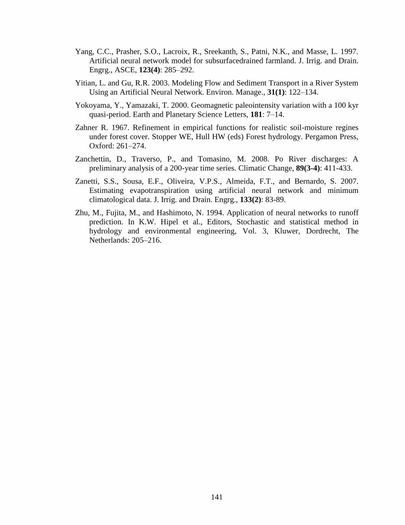
141

Yang, C.C., Prasher, S.O., Lacroix, R., Sreekanth, S., Patni, N.K., and Masse, L. 1997.

Artificial neural network model for subsurfacedrained farmland. J. Irrig. and Drain.

Engrg., ASCE, 123(4): 285–292.

Yitian, L. and Gu, R.R. 2003. Modeling Flow and Sediment Transport in a River System

Using an Artificial Neural Network. Environ. Manage., 31(1): 122–134.

Yokoyama, Y., Yamazaki, T. 2000. Geomagnetic paleointensity variation with a 100 kyr

quasi-period. Earth and Planetary Science Letters, 181: 7–14.

Zahner R. 1967. Refinement in empirical functions for realistic soil-moisture regines

under forest cover. Stopper WE, Hull HW (eds) Forest hydrology. Pergamon Press,

Oxford: 261–274.

Zanchettin, D., Traverso, P., and Tomasino, M. 2008. Po River discharges: A

preliminary analysis of a 200-year time series. Climatic Change, 89(3-4): 411-433.

Zanetti, S.S., Sousa, E.F., Oliveira, V.P.S., Almeida, F.T., and Bernardo, S. 2007.

Estimating evapotranspiration using artificial neural network and minimum

climatological data. J. Irrig. and Drain. Engrg., 133(2): 83-89.

Zhu, M., Fujita, M., and Hashimoto, N. 1994. Application of neural networks to runoff

prediction. In K.W. Hipel et al., Editors, Stochastic and statistical method in

hydrology and environmental engineering, Vol. 3, Kluwer, Dordrecht, The

Netherlands: 205–216.

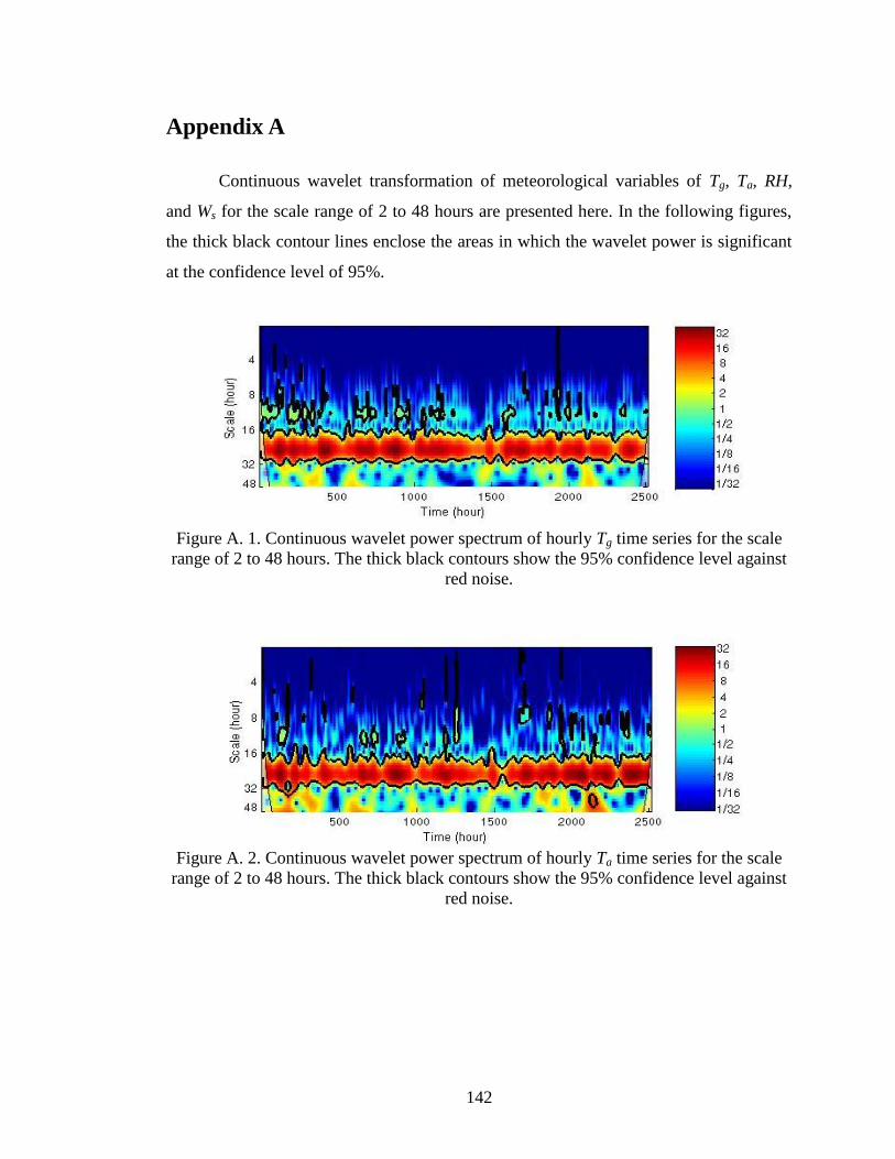
142

Appendix A

Continuous wavelet transformation of meteorological variables of Tg, Ta, RH,

and Ws for the scale range of 2 to 48 hours are presented here. In the following figures,

the thick black contour lines enclose the areas in which the wavelet power is significant

at the confidence level of 95%.

Figure A. 1. Continuous wavelet power spectrum of hourly Tg time series for the scale

range of 2 to 48 hours. The thick black contours show the 95% confidence level against

red noise.

Figure A. 2. Continuous wavelet power spectrum of hourly Ta time series for the scale


red noise.

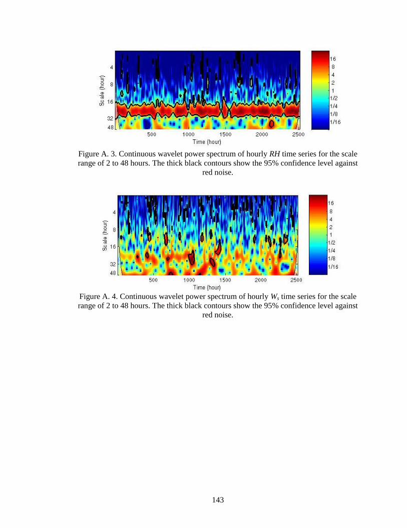
143

Figure A. 3. Continuous wavelet power spectrum of hourly RH time series for the scale


red noise.

Figure A. 4. Continuous wavelet power spectrum of hourly Ws time series for the scale


red noise.

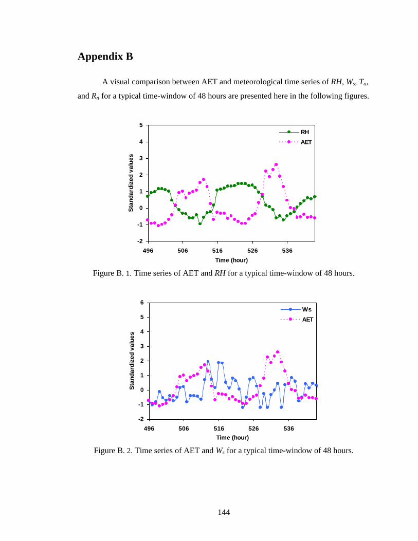
144

Appendix B

A visual comparison between AET and meteorological time series of RH, Ws, Ta,

and Rn for a typical time-window of 48 hours are presented here in the following figures.

Figure B. 1. Time series of AET and RH for a typical time-window of 48 hours.

Figure B. 2. Time series of AET and Ws for a typical time-window of 48 hours.

-2

-1

0

1

2

3

4

5

496 506 516 526 536

Time (hour)

Sta

nd

ard

ize

d v

alu

es

RH

AET

-2

-1

0

1

2

3

4

5

6

496 506 516 526 536

Time (hour)

Sta

nd

ard

ize

d v

alu

es

Ws

AET

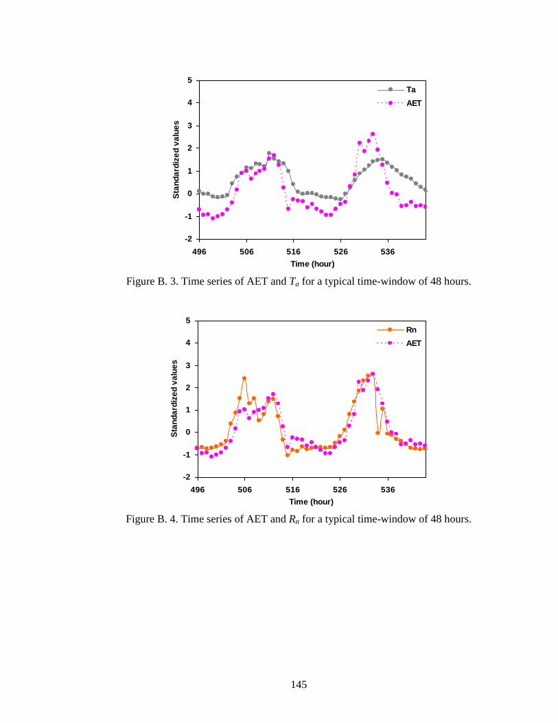
145

Figure B. 3. Time series of AET and Ta for a typical time-window of 48 hours.

Figure B. 4. Time series of AET and Rn for a typical time-window of 48 hours.

-2

-1

0

1

2

3

4

5

496 506 516 526 536

Time (hour)

Sta

nd

ard

ize

d v

alu

es

Ta

AET

-2

-1

0

1

2

3

4

5

496 506 516 526 536

Time (hour)

Sta

nd

ard

ize

d v

alu

es

Rn

AET

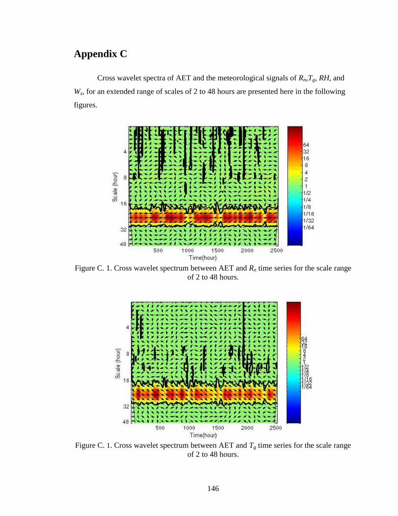
146

Appendix C

Cross wavelet spectra of AET and the meteorological signals of Rn,Tg, RH, and

Ws, for an extended range of scales of 2 to 48 hours are presented here in the following

figures.

Figure C. 1. Cross wavelet spectrum between AET and Rn time series for the scale range

of 2 to 48 hours.

Figure C. 1. Cross wavelet spectrum between AET and Tg time series for the scale range

of 2 to 48 hours.

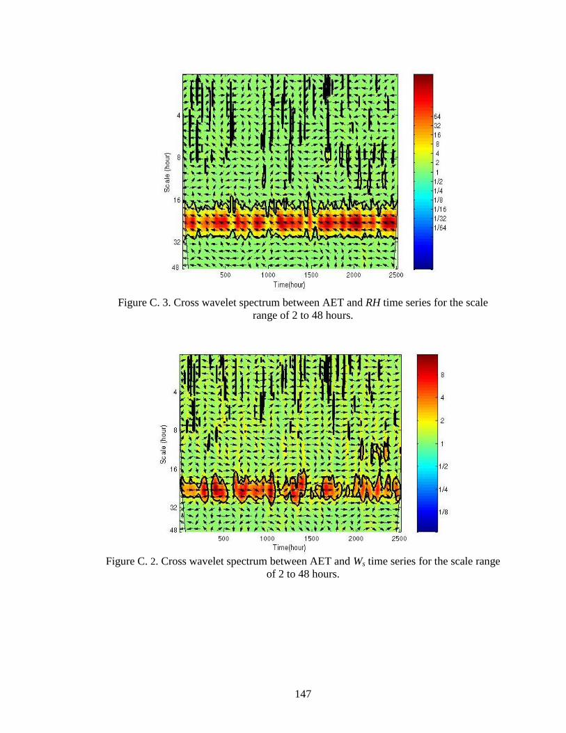
147

Figure C. 3. Cross wavelet spectrum between AET and RH time series for the scale

range of 2 to 48 hours.

Figure C. 2. Cross wavelet spectrum between AET and Ws time series for the scale range

of 2 to 48 hours.

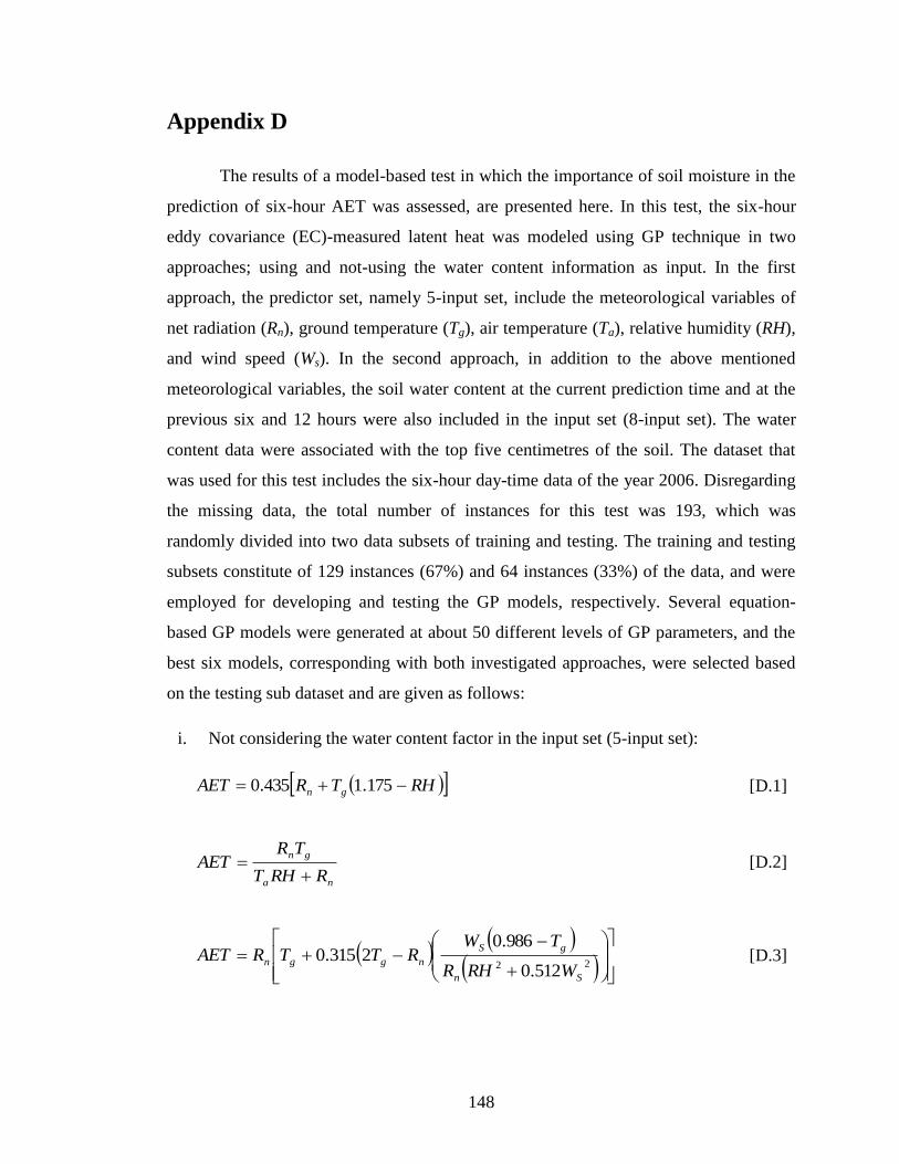
148

Appendix D

The results of a model-based test in which the importance of soil moisture in the

prediction of six-hour AET was assessed, are presented here. In this test, the six-hour

eddy covariance (EC)-measured latent heat was modeled using GP technique in two

approaches; using and not-using the water content information as input. In the first

approach, the predictor set, namely 5-input set, include the meteorological variables of

net radiation (Rn), ground temperature (Tg), air temperature (Ta), relative humidity (RH),

and wind speed (Ws). In the second approach, in addition to the above mentioned

meteorological variables, the soil water content at the current prediction time and at the

previous six and 12 hours were also included in the input set (8-input set). The water

content data were associated with the top five centimetres of the soil. The dataset that

was used for this test includes the six-hour day-time data of the year 2006. Disregarding

the missing data, the total number of instances for this test was 193, which was

randomly divided into two data subsets of training and testing. The training and testing

subsets constitute of 129 instances (67%) and 64 instances (33%) of the data, and were

employed for developing and testing the GP models, respectively. Several equation-

based GP models were generated at about 50 different levels of GP parameters, and the

best six models, corresponding with both investigated approaches, were selected based

on the testing sub dataset and are given as follows:

i. Not considering the water content factor in the input set (5-input set):

RHTRAET gn 175.1435.0 [D.1]

na

gn

RRHT

TRAET

[D.2]

22 512.0

986.02315.0

Sn

gS

nggnWRHR

TWRTTRAET [D.3]

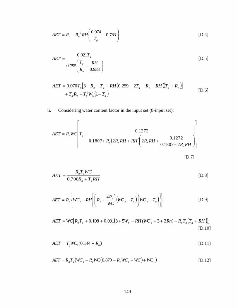
149

783.0

974.02

g

nnT

RHRRAET [D.4]

938.0795.0

921.0

RH

R

T

TAET

n

g

g [D.5]

gSgng

ngnggng

TWTRT

RTRHRTRHTRTAET

1

2259.03076.0

2 [D.6]

ii. Considering water content factor in the input set (8-input set):

RHRRHRRHRHRR

TWCRAET

n

nnn

gn

21807.0

1272.0221807.0

1272.0

[D.7]

RHTR

WCTRAET

an

gn

708.0 [D.8]

gg

n

nn TWCTWCWC

RRRHWCRAET 22

2

1

4 [D.9]

RHTTRRnWCRHWTRWCAET ggnSgn )23(53031.0108.0 2

[D.10]

)144.0(1 ng RWCTAET [D.11]

111 879.0 WCWCWCRWCRWCTRAET nngn [D.12]

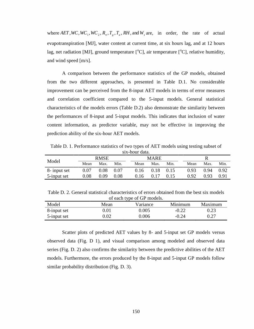
150

where sagn WRHTTRWCWCWCAET and , , , , , , ,, 21 are, in order, the rate of actual

evapotranspiration [MJ], water content at current time, at six hours lag, and at 12 hours

lag, net radiation [MJ], ground temperature [oC], air temperature [

oC], relative humidity,

and wind speed [m/s].

A comparison between the performance statistics of the GP models, obtained

from the two different approaches, is presented in Table D.1. No considerable

improvement can be perceived from the 8-input AET models in terms of error measures

and correlation coefficient compared to the 5-input models. General statistical

characteristics of the models errors (Table D.2) also demonstrate the similarity between

the performances of 8-input and 5-input models. This indicates that inclusion of water

content information, as predictor variable, may not be effective in improving the

prediction ability of the six-hour AET models.

Table D. 1. Performance statistics of two types of AET models using testing subset of

six-hour data.

Model RMSE MARE R

Mean Max. Min. Mean Max. Min. Mean Max. Min.

8- input set 0.07 0.08 0.07 0.16 0.18 0.15 0.93 0.94 0.92

5-input set 0.08 0.09 0.08 0.16 0.17 0.15 0.92 0.93 0.91

Table D. 2. General statistical characteristics of errors obtained from the best six models

of each type of GP models.

Model Mean Variance Minimum Maximum

8-input set 0.01 0.005 -0.22 0.23

5-input set 0.02 0.006 -0.24 0.27

Scatter plots of predicted AET values by 8- and 5-input set GP models versus

observed data (Fig. D 1), and visual comparison among modeled and observed data

series (Fig. D. 2) also confirms the similarity between the predictive abilities of the AET

models. Furthermore, the errors produced by the 8-input and 5-input GP models follow

similar probability distribution (Fig. D. 3).

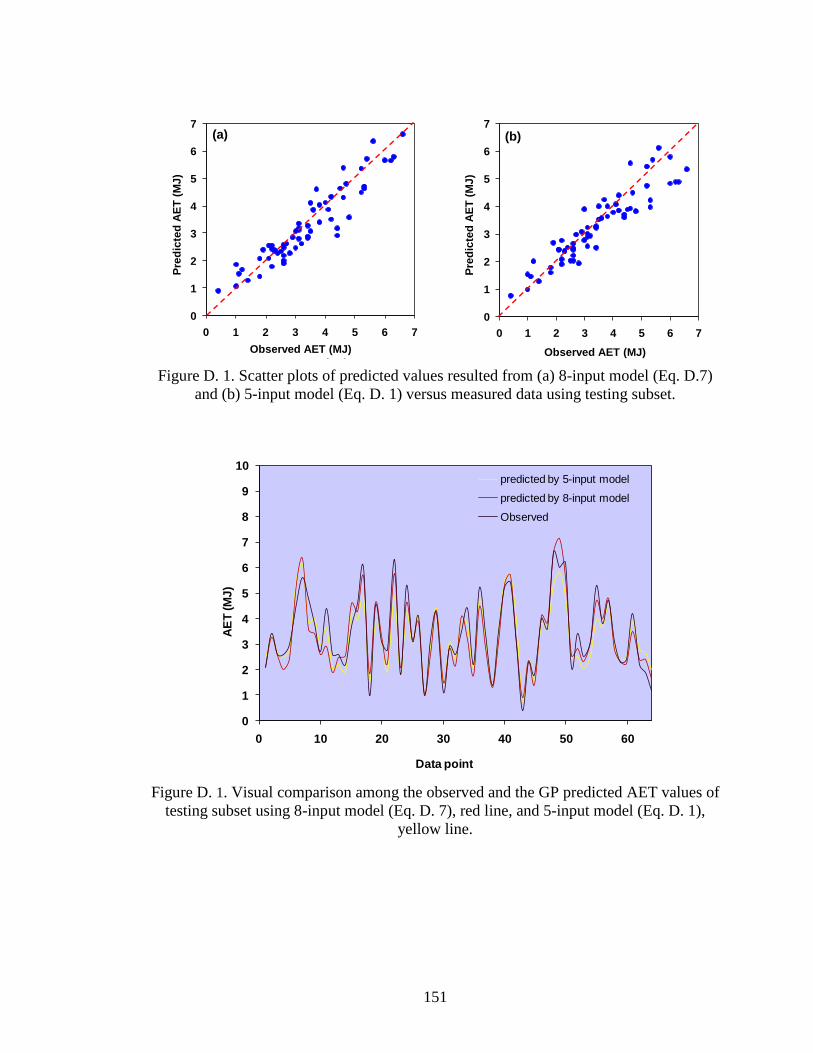
151

Figure D. 1. Scatter plots of predicted values resulted from (a) 8-input model (Eq. D.7)

and (b) 5-input model (Eq. D. 1) versus measured data using testing subset.

Figure D. 1. Visual comparison among the observed and the GP predicted AET values of

testing subset using 8-input model (Eq. D. 7), red line, and 5-input model (Eq. D. 1),

yellow line.

0

1

2

3

4

5

6

7

0 1 2 3 4 5 6 7

Pre

dic

ted

LE

(M

J)

observed LE (MJ)

model with 5-inputmodel with 5-input

0

1

2

3

4

5

6

7

0 1 2 3 4 5 6 7

Pre

dic

ted

LE

(M

J)

observed LE(MJ)

8 input (With WC) Eq.448 input …

Pre

dic

ted

AE

T (

MJ

)

Pre

dic

ted

AE

T (

MJ

)

Observed AET (MJ) Observed AET (MJ)

(a) (b)

0

1

2

3

4

5

6

7

0 1 2 3 4 5 6 7

Pre

dic

ted

LE

(M

J)

observed LE (MJ)


0

1

2

3

4

5

6

7

0 1 2 3 4 5 6 7

Pre

dic

ted

LE

(M

J)

observed LE(MJ)


Pre

dic

ted

AE

T (

MJ

)

Pre

dic

ted

AE

T (

MJ

)


0

1

2

3

4

5

6

7

0 1 2 3 4 5 6 7

Pre

dic

ted

LE

(M

J)

observed LE (MJ)


0

1

2

3

4

5

6

7

0 1 2 3 4 5 6 7

Pre

dic

ted

LE

(M

J)

observed LE(MJ)


Pre

dic

ted

AE

T (

MJ

)

Pre

dic

ted

AE

T (

MJ

)


(a) (b)

0

1

2

3

4

5

6

7

8

9

10

0 10 20 30 40 50 60

AE

T (M

J)

Data point

predicted by 5-input model

predicted by 8-input model

Observed

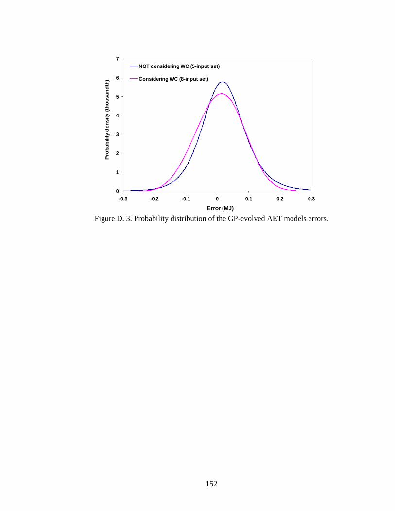
152

Figure D. 3. Probability distribution of the GP-evolved AET models errors.

0

1

2

3

4

5

6

7

-0.3 -0.2 -0.1 0 0.1 0.2 0.3

Pro

ba

bilit

y d

en

sit

y (

tho

us

an

dth

)

Error

NOT considering WC (5-input set)

Considering WC (8-input set)

Error (MJ)

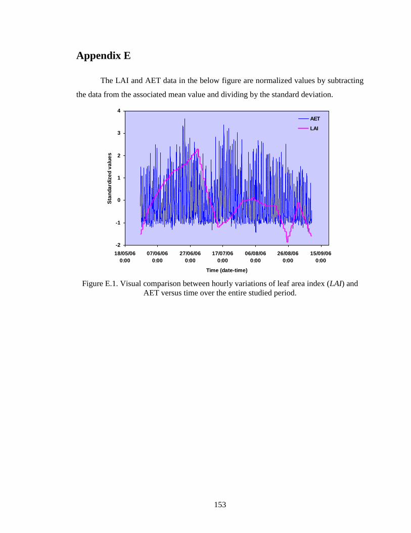
153

Appendix E

The LAI and AET data in the below figure are normalized values by subtracting

the data from the associated mean value and dividing by the standard deviation.

Figure E.1. Visual comparison between hourly variations of leaf area index (LAI) and

AET versus time over the entire studied period.

-2

-1

0

1

2

3

4

18/05/06

0:00

07/06/06

0:00

27/06/06

0:00

17/07/06

0:00

06/08/06

0:00

26/08/06

0:00

15/09/06

0:00

Time (date-time)

Sta

nd

ard

ize

d v

alu

es

AET

LAI

Documents

MODELING AND ANALYSIS OF ACTUAL …