Embed Size (px)
Citation preview

Model Order Reduction of Continuous LTI Large
Descriptor System Using LRCF-ADI and Square
Root Balanced Truncation
Mehrab Hossain Likhon, Shamsil Arifeen, and Mohammad Sahadet Hossain
Abstract− In this paper, we analyze a linear time invariant
(LTI) descriptor system of large dimension. Since these systems
are difficult to simulate, compute and store, we attempt to
reduce this large system using Low Rank Cholesky Factorized
Alternating Directions Implicit (LRCF-ADI) iteration followed
by Square Root Balanced Truncation. LRCF-ADI solves the
dual Lyapunov equations of the large system and gives low-
rank Cholesky factors of the gramians as the solution. Using
these cholesky factors, we compute the Hankel singular values
via singular value decomposition. Later, implementing square
root balanced truncation, the reduced system is obtained. The
bode plots of original and lower order systems are used to show
that the magnitude and phase responses are same for both the
systems.
Keywords− LTI descriptor system, suboptimal shift parameter,
Lyapunov equation, low rank Cholesky factor alternating
direction implicit (LRCF-ADI), square root balanced
truncation.
I. INTRODUCTION
1With the advancement of technology, our lives are
getting simpler but systems around us are getting compact
and complex. Often, these complex systems, such as multi
body dynamics with constrains, electrical circuit simulation,
fluid flow dynamics, VLSI chip design are modeled as
Descriptor systems or generalized state space systems of
very large dimension. Even though, the computational speed
and performance of the contemporary computers are
enhanced, simulation and optimization of such large-scale
systems still remain difficult due to storage limitations and
expensive computations [1]. In order to eliminate this
problem, reduction of such large systems is mandatory.
Large systems are generally comprised of sparse matrices
[2]. The system was reduced after implementing several
numerical methods namely Arnoldi iteration for calculating
the Ritz values, ADI min-max problem to get the shift
parameters heuristically, then low-rank Cholesky factor
alternating directions implicit iteration for low rank
Mehrab Hossain Likhon is with the Electrical and Computer
Engineering Department, North South University, Basundhara R/A, Dhaka
1229, Bangladesh (e-mail: [email protected])
Shamsil Arifeen is with the Electrical and Computer Engineering
Department, North South University, Basundhara R/A, Dhaka 1229,
Bangladesh (e-mail: [email protected])
Mohammed Sahadet Hossain is with the Mathematics and Physics
Department, North South University, Basundhara R/A, Dhaka 1229,
Bangladesh (e-mail: [email protected])
approximations of the cholesky factors of the controllability
and observability Gramians of the system. Finally, by using
the Hankel Singular Values, calculated from singular value
decomposition of the product of the approximated cholesky
factors, were able to discard the states of the system that are
both difficult to observe and control. Only the Hankel
Singular Values of large magnitude determine the dimension
of the reduced system, since these values describe the
dominant dynamics of the large system. Thus using
projection matrices, the original system matrices are
transformed into reduced dimension, same as the quantity of
the Hankel Singular Values retained. However, the major
difficulty while conducting this research was in calculating
the optimal shift parameters.
II. MATHEMATICAL MODEL
Our system of concern is a continuous Linear Time
Invariant (LTI) system of Descriptor form and can be
represented as follows:
𝐸�̇�(𝑡) = 𝐴𝑥(𝑡) + 𝐵𝑢(𝑡), 𝑦(𝑡) = 𝐶𝑥(𝑡) + 𝐷𝑢(𝑡).
(1)
Where, 𝐸 ∈ ℝ𝑛×𝑛, 𝐴 ∈ ℂ𝑛×𝑛, 𝐵 ∈ ℝ𝑛×𝑚, 𝐶 ∈ ℝ𝑝×𝑛, 𝐷 ∈ ∅.
Here, 𝐸 is sparse, non-singular (i.e. invertible) and is a
symmetric positive definite matrix, like most other large
systems, indicating that all the variables are state variables
and cannot be neglected [3]. If E = I, then the LTI
continuous system is a standard state space system, else, it is
a descriptor or generalized state space system. 𝐴 is a
complex, sparse Hurwitz matrix (i.e. all the real parts of the
eigenvalues of 𝐴 are negative). Both 𝐴 and 𝐸 are tridiagonal
for this system. 𝐵 is the m-dimensional input vector, 𝐶 is the
p-dimensional output vector, As this is not a closed loop
system, so 𝐷 is null, 𝑥(𝑡) is the n-dimensional
descriptor/state vector of the system and 𝑢(𝑡) and 𝑦(𝑡) are
the system input and output respectively. This is a single-
input-single-output (SISO) system so, 𝑚 = 𝑝 =1. As,
𝐸, 𝐴, 𝐵, 𝐶 are constant matrices and independent of time,
hence this system is linear and time invariant. As rank
[𝛼𝐸 − 𝛽𝐴, 𝐵] =rank [𝛼𝐸𝑇 − 𝛽𝐴𝑇 , 𝐶𝑇] = 𝑛, for ∀(𝛼, 𝛽) ∈(ℂ × ℂ)\{0,0} for this system, hence it is completely
controllable and observable [1] and is an important criterion
for executing balanced truncation [4]. For generalized state
space models like this, the eigenvalues of the matrix pair (E,
A), i.e. pencil (𝜆𝐸 − 𝐴), determines the stability of the
Proceedings of the World Congress on Engineering 2015 Vol I WCE 2015, July 1 - 3, 2015, London, U.K.
ISBN: 978-988-19253-4-3 ISSN: 2078-0958 (Print); ISSN: 2078-0966 (Online)
WCE 2015
system. This pencil must be regular, i.e. det(𝜆𝐸 − 𝐴) ≠ 0
and all the eigenvalues must lie on the left half plane to
ensure that the LRCF-ADI iteration converges.
After undergoing the model order reduction process,
this descriptor system will be approximated by a reduced-
order system as:
𝐸𝑟�̇�𝑟(𝑡) = 𝐴𝑟𝑥𝑟(𝑡) + 𝐵𝑟𝑢(𝑡),
𝑦(𝑡) = 𝐶𝑟𝑥(𝑡).
(2)
Here, 𝐸𝑟 ∈ ℝ𝑙×𝑙 , 𝐴𝑟 ∈ ℂ𝑙×𝑙 , 𝐵𝑟 ∈ ℝ𝑙×𝑚, 𝐶𝑟 ∈ ℝ𝑝×𝑙 and
𝑙 ≪ 𝑛. These are the system matrices of the reduced system
where 𝑙 is the dimension of the reduced system.
III. PRELIMINARIES
A. Block Arnoldi Iteration
As mentioned in [5], Arnoldi method creates an
orthogonal basis of a Krylov subspace represented by the
orthonormal matrix, 𝑉 = (𝑣1, 𝑣2, 𝑣3 … … … … , 𝑣𝑘) ∈ ℂ𝑛×𝑘
such that 𝑉∗𝑉 = 𝐼, where 𝑉∗ is the conjugate transpose of 𝑉.
Here 𝑠𝑝𝑎𝑛(𝑣1, 𝑣2, 𝑣3 … , 𝑣𝑘) ≅ 𝛫𝜅(𝐹, 𝑏) means
𝑠𝑝𝑎𝑛(𝑣1, 𝑣2, 𝑣3 … , 𝑣𝑘) ≅ 𝑠𝑝𝑎𝑛(𝑏, 𝐹𝑏, 𝐹2𝑏, … , 𝐹𝑘−1𝑏)
Where, 𝐹 = 𝐸−1𝐴, and 𝑏 is a random initial vector,
required to start the Arnoldi iteration. The generalized
eigenvalues can be approximated from the eigenvalues of
the Hessenberg matrix 𝐻 (i.e. Ritz values) provided that the
same eigenvector is present in the subspace, where 𝐻 =𝑉∗𝐹𝑉 and 𝐻 ∈ ℂ𝑘×𝑘 and is generated as a by-product of the
Arnoldi iteration. The algorithm of the Arnoldi Iteration up
to k-th step is depicted in [6]. Solving the equations (3) and
(4) at each step, is the main job till the k-th step is reached.
𝐹𝑉 = 𝑉𝐻 + 𝑓𝑒𝑘 , 𝐻 = 𝑉𝑇𝐹𝑉, 𝑉𝑇𝑉 = 𝐼𝑘 , 𝑉𝑇𝑓 = 0.
(3)
(4)
𝐻 is the Hessenberg matrix and 𝑉 is the orthonormal
vector matrix and 𝑓 is the residual at each iteration and 𝑒𝑘 is
the last column of 𝐼𝑘. Arnoldi algorithm generates a
factorization of the form 𝐹𝑉𝑘 = 𝑉𝑘+1𝐻𝑘 [7]. Initially, 𝑉1 is
set as the unit vector of the initial vector, 𝑏. Then it
computes 𝐻1 = 𝑉1∗𝐹𝑉1 followed by the residual 𝑓1 = 𝐹𝑉1 −
𝑉1𝐻1 which in turn is orthogonal to 𝑉1. Thus 𝑉2 =
[𝑉1 𝑓1
||𝑓1||]. Then again 𝐻2 = 𝑉2
∗𝐹𝑉2 and 𝑅2 = 𝐹𝑉2 − 𝑉2𝐻2,
resulting in 𝑅2=[0 𝑓2] = 𝑓2𝑒2. Sequentially, 𝑉3, 𝐻3, 𝑅3 are
calculated and so are the respective matrices until the last
Arnoldi iteration step is reached to give 𝑉𝑘 and 𝐻𝑘 .
We will execute the Arnoldi iteration one more time,
using 𝐹−1 instead of 𝐹, this process is referred to as the
inverse Arnoldi iteration. From each of the Hessenberg
matrices, which are always upper triangular matrices,
obtained from the iterations, would help us in better
approximation of the large as well as the small generalized
eigenvalues of the system. In other words, smaller and the
largest eigenvalues of the pencil are approximated from the
eigenvalues of each of the Hessenberg matrices. The process
of how the eigenvalues of the system is approximated is
mentioned elaborately in [5]. At the end, we get the Ritz
values that are pretty good approximation of the significant
eigenvalues (i.e. smallest and largest ones).
B. Low-Rank Cholesky Factor ADI
The system is a model of continuous generalized
Lyapunov equation that helps to determine the asymptotic
stability of the system [8]. The generalized Lyapunov
equation is shown in (4).
𝐴𝑋𝐸𝑇 + 𝐸𝑋𝐴𝑇 = −𝐺𝐺𝑇 . (4)
We consider the solutions of the dual Lyapunov
equations in (5)
𝐴𝑃𝐸𝑇 + 𝐸𝑃𝐴𝑇 = −𝐵𝐵𝑇 , 𝐴𝑇𝑄𝐸 + 𝐸𝑇𝑄𝐴 = −𝐶𝑇𝐶.
(5)
The solutions of the equations in (5) are matrices 𝑃, the
controllability Gramian, and 𝑄, the observability Gramian
[9]. There are several methods for solving Lyapunov
equations, namely Bartel-Stewart method, alternating
direction implicit (ADI) method, Smith method, Krylov
subspace method [10]. But, LRCF-ADI gives the low-rank
approximations �̂�, �̂� instead of the full rank solutions from
the methods mentioned earlier, especially when the right
hand side of the equation has low rank. This is a major
improvement suggested in [11] and is a great advantage for
storage space and computational speed.
LRCF-ADI gives low rank approximated Cholesky
factors �̂�𝐶 and �̂�𝑂 of the controllability and observability
gramians respectively, such that
�̂� = �̂�𝐶�̂�𝐶𝑇 , �̂� = �̂�𝑂�̂�𝑂
𝑇 . (7)
Initial task is to compute optimal shift parameters,
{𝑝1, 𝑝2, 𝑝3,, … . . 𝑝𝑗}. LRCF-ADI only converges if the shift
parameters are negative, retrieved if the eigenvalues of the
pencil (𝜆𝐸 − 𝐴) are negative. These shift parameters are the
solution of rational discrete min-max problem as depicted in
[2].
𝑚𝑖𝑛
𝑝1, 𝑝2, 𝑝3,𝑝4, … . . 𝑝𝑗
𝑚𝑎𝑥𝑥𝜖ℝ
∏(𝑝𝑗 − 𝑥)
(𝑝𝑗 + 𝑥)
𝑗
𝑛=1
(8)
In (8), 𝑥 represents the set of ritz values obtained from
the Arnoldi iteration. Though, they should be a set of real
values, in this case these are complex. The process (8)
decides whether the parameters selected are optimal,
suboptimal or near-optimal. If the eigenvalues of the pencil
(𝜆𝐸 − 𝐴) are strictly real and is bounded, then it is possible
to retrieve optimal parameters. As the Ritz values are
complex, so the parameters are sub-optimal.
Once the parameter selection is complete, then the ADI
iteration is carried out, that will give �̂�𝐶 and �̂�𝑂. ADI solves
the following iterations using (5), (6)
(𝐴 + 𝑝𝑗𝐸)𝑋𝑗 −
12
= −𝐺𝐺𝑇 − 𝑋𝑗−1(𝐴𝑇 − 𝑝𝑗𝐸),
(𝐴 + 𝑝𝑗𝐸)𝑋𝑗 = −𝐺𝐺𝑇 − 𝑋𝑗 −
12
𝑇 (𝐴𝑇 − 𝑝𝑗𝐸).
(9)
These two steps are required to ensure the symmetry of
the solution, 𝑋𝑗, where j is the number of iteration steps.
Combining these two steps in (9), by substituting the first
Proceedings of the World Congress on Engineering 2015 Vol I WCE 2015, July 1 - 3, 2015, London, U.K.
ISBN: 978-988-19253-4-3 ISSN: 2078-0958 (Print); ISSN: 2078-0966 (Online)
WCE 2015
iteration of 𝑋𝑗 −
1
2
in the second one for 𝑋𝑗, we get one-step
iteration
𝑋𝑗 =
−2𝑝𝑗(𝐴 + 𝑝𝑗𝐸)
−1𝐺𝐺𝑇 (𝐴 + 𝑝𝑗𝐸)
−𝑇+(𝐴 + 𝑝𝑗𝐸)
−1
(𝐴 − 𝑝𝑗𝐸)𝑋𝑗−1 (𝐴 − 𝑝𝑗𝐸)𝑇
(𝐴 + 𝑝𝑗𝐸)−𝑇
.
(10)
Now, writing 𝑋𝑗 as the product of Cholesky factors, it
turns out to be 𝑋𝑗 = 𝑍𝑗𝑍𝑗𝑇 , now relating this factorization to
the one-step iteration above
𝑍𝑗=[√−2𝑝1 ((𝐴 + 𝑝1𝐸)−1𝐺), (𝐴 + 𝑝𝑗𝐸)−1
(𝐴 − 𝑝𝑗𝐸)𝑍𝑗−1],
Where the result of very first iteration
𝑍1
= √−2𝑝1((𝐴 + 𝑝1𝐸)−1𝐺).
At every iteration step, a new column is added to the
Cholesky factors in the following process i.e.
𝑍𝐽 = [𝑧𝐽, 𝑃𝐽−1𝑧𝐽, 𝑃𝐽−2(𝑃𝐽−1𝑧𝐽), … … , 𝑃1(𝑃2 … 𝑃𝐽−1𝑧𝐽)] ,
Where 𝑃𝑖 =√−2𝑅𝑒(𝑝𝑖)
√−2𝑅𝑒(𝑝𝑖+1) (𝐴 + 𝑝𝑖𝐸)−1 (𝐴 − 𝑝𝑖−1𝐸) .
𝑃𝑖 is the iteration step operator and the product 𝑍𝑗𝑍𝑗𝑇 is
calculated to get 𝑋𝑗, which after substitution in the equation
(4), the residual norm is checked after each iteration step.
||𝐴𝑋𝑗𝐸𝑇 + 𝐸𝑋𝑗𝐴𝑇 + 𝐺𝐺𝑇|| < 𝜀.
Until, a desired residual tolerance, 𝜀, is overcome, the steps
3 to 5 of the algorithm in [12] are repeated.
�̂� = �̂�𝐶�̂�𝐶𝑇 ,
�̂� = �̂�𝑂�̂�𝑂𝑇 .
(11)
(12)
LRCF-ADI solves (5) and (6) to give �̂�, �̂� in (11) and
(12). Which are the low-rank approximation to the
Controllability and Observability Gramians. Column
compression computes a compressed form of the Cholesky
factor using rank revealing QR decomposition [12]. Column
compression process is required in case of failure to
compute the optimal shift parameters resulting in slow
convergence with many iteration steps. This will gradually
increase the dimension of the subspace spanned by the
columns of the low-rank Cholesky factors. As a new column
is added in every iteration step to the Cholesky factor 𝑍𝑗.
These new columns occupy the memory and increases the
computational cost of the iteration. It is therefore required to
keep the factors as small in rank as possible.
C. Balanced Truncation
Balanced Truncation is an important projection method
which delivers high quality reduced models by choosing the
projection subspaces based on the Controllability and
Observability of a control system [13], by truncating low
energy states of the system corresponding to the small
Hankel singular values. [14]
Among couple of methods, Square Root Balanced
Truncation (SRBT) is used here for truncating the system.
SRBT algorithms often provide more accurate reduced-
order models in the presence of rounding errors [15]. This
method needs the Hankel singular values, and low-rank
Cholesky factors in (11) and (12), obtained from LRCF-ADI
iteration. These are considered as a measure of energy for
each state in the system. They are the basis of balanced
model reduction, in which low energy states are identified
from the high energy states and are truncated.
Hankel singular values are calculated as the square
roots of the eigenvalues for the product of the low-rank
controllability and the observability Gramians. These
Hankel singular values 𝜎𝑖, are the diagonal entries of the
Hankel matrix Σ.
𝜎𝑖(𝛴) = √𝜆𝑖(�̂��̂�) ,
The Hankel singular values calculated from singular
value decomposition of the product of the low-rank
Cholesky factors and the matrix 𝐸 shown in (13), truncates
the states of the large system that are both difficult to
observe and control. This factorization is known as full
singular value decomposition [14].
𝑈𝛴𝑉𝑇 = 𝑠𝑣𝑑(�̂�𝑂𝑇𝐸�̂�𝐶) . (13)
Where 𝑈 𝜖 ℝ𝑚 𝑥 𝑚 is a unitary matrix, and UUT = VVT = I
and 𝛴 𝜖 ℝ𝑚 𝑥 𝑛 is a diagonal matrix with positive real
numbers, and 𝑉 𝜖 ℝ𝑛 𝑥 𝑛 is another unitary matrix.
𝑉𝑇 denotes the conjugate transpose of 𝑉. This factorization
is called a singular value decomposition and the diagonal
entries of Σ are known as the singular values.
A tolerance level is necessary so that the Hankel
singular values less than that in magnitude will be truncated.
Now, for instance if the number of Hankel singular values
above the tolerance level is 𝑞, then the first 𝑞 columns from
U and V will be retained and can be denoted as 𝑈𝐶 and 𝑉𝐶
respectively (𝑈𝐶 𝜖 ℝ𝑚 × 𝑞 and 𝑉𝐶 𝜖 ℝ𝑛 × 𝑞). After truncating
the lower Hankel values and retaining the first 𝑞 values from
the diagonal singular matrix, 𝛴 denoting the reduced matrix
as 𝛴𝐶, where, 𝛴𝐶 = 𝑑𝑖𝑎𝑔(𝜎1 … … … … 𝜎𝑞) 𝜖 ℝ𝑞 𝑥 𝑞 then we
can write this SVD as thin SVD or economic SVD [14],
[16].
The square root balanced truncation is successful if the
error between the transfer function of both the systems is
less than twice the sum of the truncated Hankel values
𝜎𝑞+1, … … … 𝜎𝑛 and 𝑞 < 𝑛 [14].
‖𝐻(𝑠) − �̂�(𝑠)‖ℋ∞
≤ 2(𝜎𝑞+1 + ⋯ + ⋯ + 𝜎𝑛).
These reduced Hankel singular values are used to get the
non-singular transformation/projection matrices 𝑇𝐿 and 𝑇𝑅
such that
𝑇𝐿 = 𝑍𝑂𝑈𝐶𝛴𝐶−1/2
and 𝑇𝑅 = 𝑍𝐶𝑉𝐶𝛴𝐶−1/2
.
Using these projection matrices (i.e. transformation
matrices), the original system matrices are transformed into
reduced order as shown in (14)
Proceedings of the World Congress on Engineering 2015 Vol I WCE 2015, July 1 - 3, 2015, London, U.K.
ISBN: 978-988-19253-4-3 ISSN: 2078-0958 (Print); ISSN: 2078-0966 (Online)
WCE 2015
𝐸𝑟 = 𝑇𝐿𝑇 𝐸 𝑇𝑅 ,
𝐴𝑟 = 𝑇𝐿𝑇 𝐴 𝑇𝑅 ,
𝐵𝑟 = 𝑇𝐿𝑇 𝐵,
𝐶𝑟 = 𝐶 𝑇𝑅 .
(14)
After undergoing the model order reduction process,
this descriptor system will be approximated by a reduced-
order system as
𝐸𝑟�̇�𝑟(𝑡) = 𝐴𝑟𝑥𝑟(𝑡) + 𝐵𝑟𝑢(𝑡), 𝑦(𝑡) = 𝐶𝑟𝑥(𝑡).
(15)
IV. NUMERICAL RESULT
To compute these Hessenberg matrices H, we used the
Block Arnoldi method and inverse Arnoldi method. Here the
Arnoldi process returns larger eigenvalues and Inverse
Arnoldi process returns the smaller eigenvalues of the
Hessenberg matrices, H, for the respective cases via QR
algorithm.
Numbers of steps for Arnoldi process and inverse
Arnoldi processes are determined as 𝑘𝑝=35 and 𝑘𝑚=35
respectively. Desired number of shift parameters for LRCF-
ADI are selected to be, 𝑙𝑜=25. The values selected are
relatively high due to the complexity and large
dimensionality of the system [11].
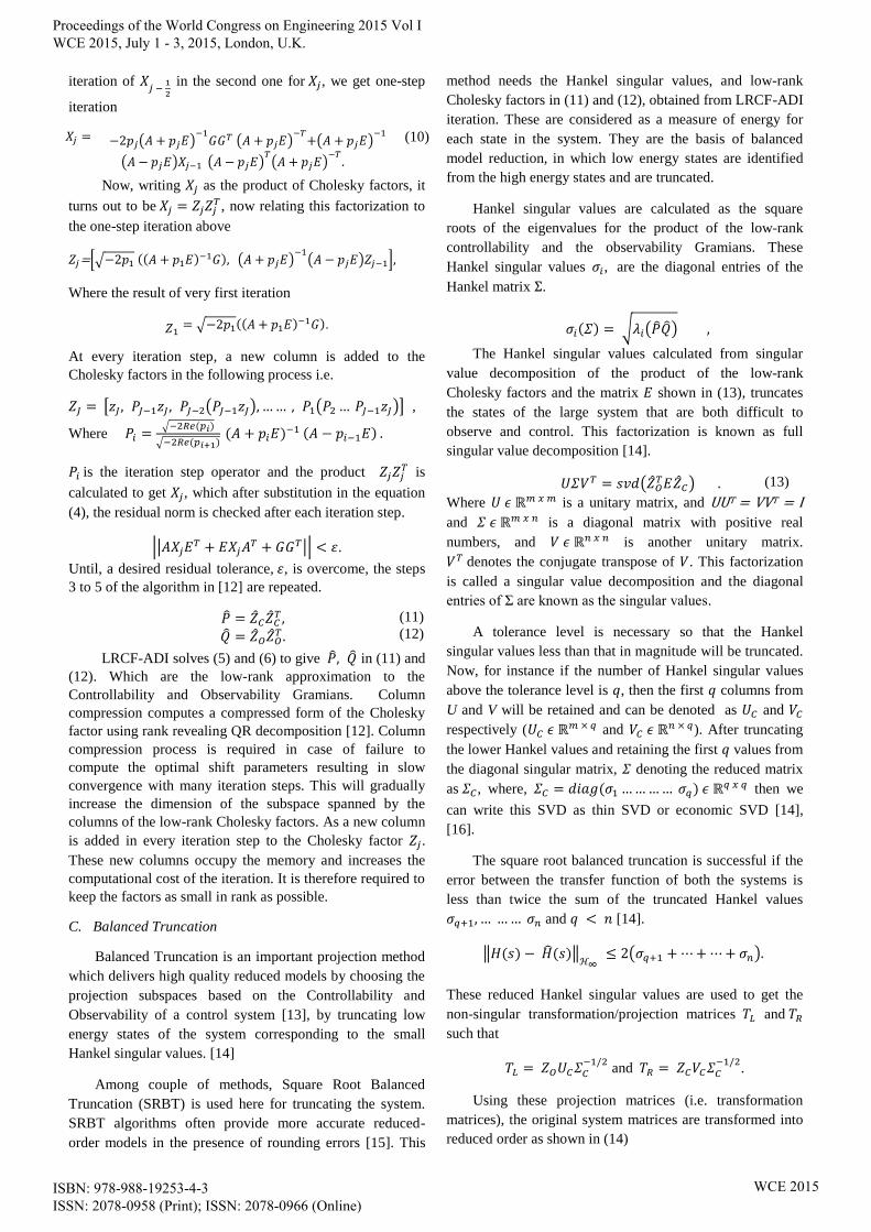
Using the Heuristic Algorithm, ADI min max rational
problem computes the shift parameters heuristically from
the Ritz values. These were sub-optimal due to the Ritz
values being complex quantities. These parameters were not
close to the largest Ritz values as shown in Fig. 1.
Fig. 1: Suboptimal shift parameters and Ritz values
We made a model of our system with Lyapunov
equations (5) and (6) and solved these to get the low-rank
Cholesky factors of controllability gramian and of
observability gramian, �̂�𝐶 and �̂�𝑂 respectively
where �̂�𝐶 𝜖 ℂ645 𝑥 22 and �̂�𝑂 𝜖 ℂ645 𝑥 21. The columns of
the Cholesky factors of the controllability and observability
gramians are 22 and 21 respectively; this is because the
LRCF-ADI iteration converged to a residual norm of 10-5 by
21 iteration steps. In addition, column compression
frequency of 20 was used along with the column
compression tolerance of 10-5.
Later, using these cholesky factors, we computed
Hankel singular values by singular value decomposition
method.
𝑈𝛴𝑉𝑇 = 𝑠𝑣𝑑(𝑍𝑂𝑇𝐸𝑍𝐶). (17)
Here 𝑈 𝜖 ℝ21 𝑥 21 , 𝛴 𝜖 ℝ21 𝑥 22 , 𝑉 𝜖 ℝ22 𝑥 22 .
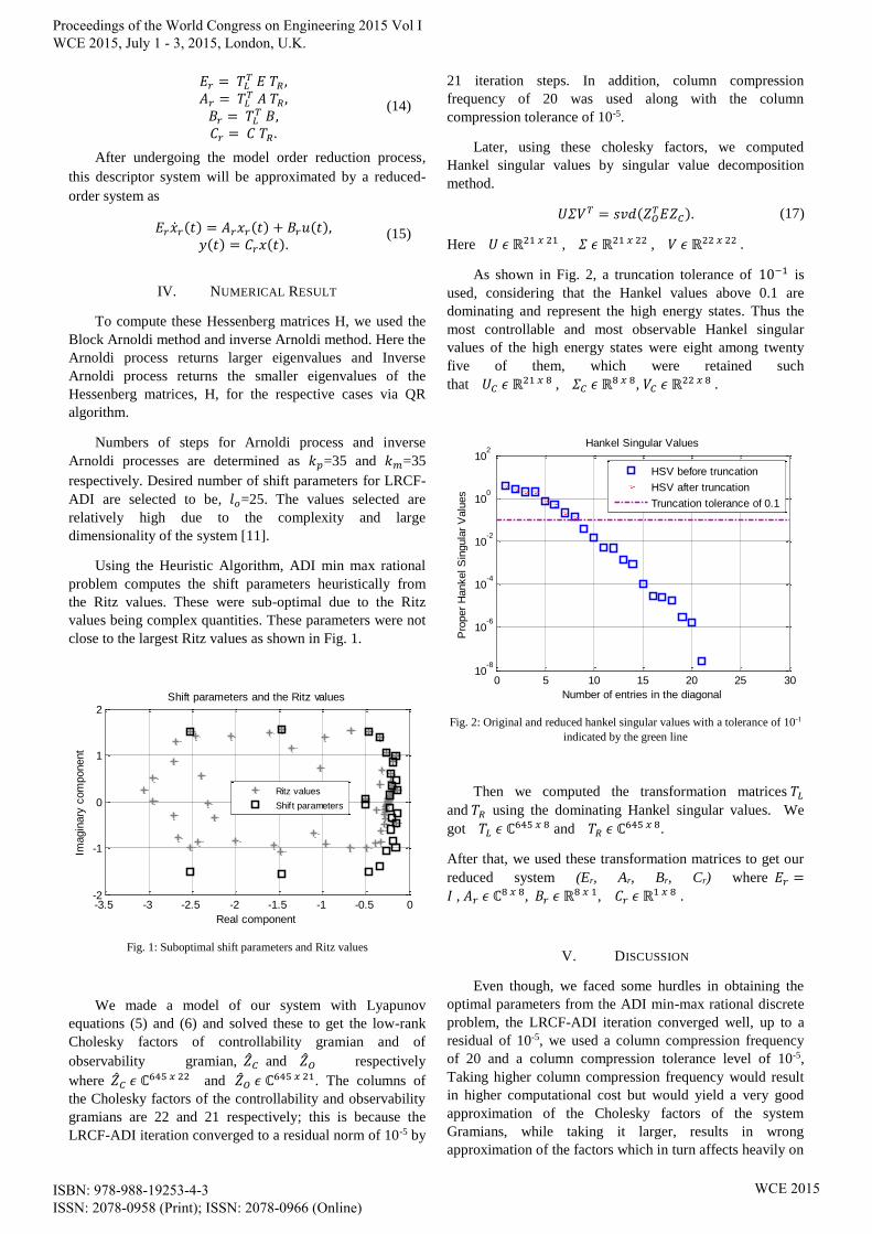
As shown in Fig. 2, a truncation tolerance of 10−1 is
used, considering that the Hankel values above 0.1 are
dominating and represent the high energy states. Thus the
most controllable and most observable Hankel singular
values of the high energy states were eight among twenty
five of them, which were retained such
that 𝑈𝐶 𝜖 ℝ21 𝑥 8 , 𝛴𝐶 𝜖 ℝ8 𝑥 8, 𝑉𝐶 𝜖 ℝ22 𝑥 8 .
Fig. 2: Original and reduced hankel singular values with a tolerance of 10-1
indicated by the green line
Then we computed the transformation matrices 𝑇𝐿
and 𝑇𝑅 using the dominating Hankel singular values. We
got 𝑇𝐿 𝜖 ℂ645 𝑥 8 and 𝑇𝑅 𝜖 ℂ645 𝑥 8.
After that, we used these transformation matrices to get our
reduced system (Er, Ar, Br, Cr) where 𝐸𝑟 =
𝐼 , 𝐴𝑟 𝜖 ℂ8 𝑥 8, 𝐵𝑟 𝜖 ℝ8 𝑥 1, 𝐶𝑟 𝜖 ℝ1 𝑥 8 .
V. DISCUSSION
Even though, we faced some hurdles in obtaining the
optimal parameters from the ADI min-max rational discrete
problem, the LRCF-ADI iteration converged well, up to a
residual of 10-5, we used a column compression frequency
of 20 and a column compression tolerance level of 10-5,
Taking higher column compression frequency would result
in higher computational cost but would yield a very good
approximation of the Cholesky factors of the system
Gramians, while taking it larger, results in wrong
approximation of the factors which in turn affects heavily on
-3.5 -3 -2.5 -2 -1.5 -1 -0.5 0-2
-1
0
1
2
Real component
Imagin
ary
com
ponent
Shift parameters and the Ritz values
Ritz values
Shift parameters
0 5 10 15 20 25 3010
-8
10-6
10-4
10-2
100
102
Number of entries in the diagonal
Pro
per
Hankel S
ingula
r V
alu
es
Hankel Singular Values
HSV before truncation
HSV after truncation
Truncation tolerance of 0.1
Proceedings of the World Congress on Engineering 2015 Vol I WCE 2015, July 1 - 3, 2015, London, U.K.
ISBN: 978-988-19253-4-3 ISSN: 2078-0958 (Print); ISSN: 2078-0966 (Online)
WCE 2015
the reduced model approximation. Thus 20, was chosen as
the column compression frequency as a trade-off between
the two ends. Moreover, the column compression frequency
should not exceed the number of columns of the Cholesky
factors. In that case, column compression would not be
performed at all. Thus it is absolutely necessary to consider
the column compression to be lower than 21.
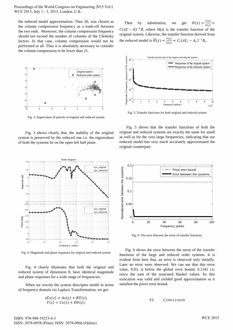
Fig. 3: Eigenvalues of pencils of original and reduced system
Fig. 3 shows clearly that, the stability of the original
system is preserved by the reduced one i.e. the eigenvalues
of both the systems lie on the open left half plane.
Fig. 4: Magnitude and phase responses for original and reduced system
Fig. 4 clearly illustrates that both the original and
reduced system of dimension 8, have identical magnitude
and phase responses for a wide range of frequencies.
When we rewrite the system descriptor model in terms
of frequency domain via Laplace Transformation; we get:
𝑠𝐸𝑥(𝑠) = 𝐴𝑥(𝑠) + 𝐵𝑈(𝑠), 𝑌(𝑠) = 𝐶𝑥(𝑠) + 𝐷𝑈(𝑠).
Then by substitution, we get 𝐻(𝑠) =𝑌(𝑠)
𝑈(𝑠)=
𝐶(𝑠𝐸 − 𝐴)−1𝐵, where H(s) is the transfer function of the
original system. Likewise, the transfer function derived from
the reduced model is 𝐻(𝑠) =𝑌(𝑠)
𝑈(𝑠)= 𝐶𝑟(𝑠𝐸𝑟 − 𝐴𝑟)−1𝐵𝑟 .
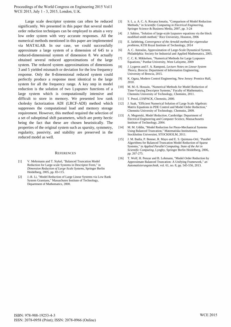
Fig. 5: Transfer functions for both original and reduced system
Fig. 5 shows that the transfer functions of both the
original and reduced systems are exactly the same for small
as well as for the very large frequencies, indicating that our
reduced model has very much accurately approximated the
original counterpart.
Fig. 6: The error between the norm of transfer functions.
Fig. 6 shows the error between the norm of the transfer
functions of the large and reduced order systems. It is
evident from here that, an error is observed only initially.
Later no error were observed. We can see that this error
value, 0.03, is below the global error bound, 0.1341 i.e.
twice the sum of the truncated Hankel values. So this
truncation was valid and yielded good approximation as it
satisfied the priori error bound.
VI. CONCLUSION
-6 -5 -4 -3 -2 -1 0-6
-4
-2
0
2
4
6
Original system
Reduced order system
-30
-20
-10
0
10
20
Magnitude (
dB
)
10-3
10-2
10-1
100
101
102
-90
0
90
180
270
360
450
Phase (
deg)
Bode Diagram
Frequency (rad/s)
sys_original
sys_reduced
sys_original
sys_reduced
0 1 2 3 4 5 6 7 8 9 10
x 104
10-6
10-4
10-2
100
102
Transfer function plot of the original and reduced system
Frequency (rad/sec)Magnitude o
f fr
equency r
esponse o
f th
e s
yste
ms
Response of the original system
Response of the reduced system
0 20 40 60 80 100
0
0.05
0.1
0.15
0.2
Frequency points
Norm
aliz
ed e
rror
betw
een t
he s
yste
ms
Priori error bound
Error between the systems
Proceedings of the World Congress on Engineering 2015 Vol I WCE 2015, July 1 - 3, 2015, London, U.K.
ISBN: 978-988-19253-4-3 ISSN: 2078-0958 (Print); ISSN: 2078-0966 (Online)
WCE 2015
Large scale descriptor systems can often be reduced
significantly. We presented in this paper that several model
order reduction techniques can be employed to attain a very
low order system with very accurate responses. All the
numerical methods mentioned in this paper are implemented
via MATALAB. In our case, we could successfully
approximate a large system of a dimension of 645 to a
reduced-dimensional system of dimension 8. We actually
obtained several reduced approximations of the large
system. The reduced system approximations of dimensions
3 and 5 yielded mismatch or deviation for the low frequency
response. Only the 8-dimensional reduced system could
perfectly produce a response most identical to the large
system for all the frequency range. A key step in model
reduction is the solution of two Lyapunov functions of a
large system which is computationally intensive and
difficult to store in memory. We presented low rank
cholesky factorization ADI (LRCF-ADI) method which
suppresses the computational load and memory storage
requirement. However, this method required the selection of
a set of suboptimal shift parameters, which are pretty hectic
being the fact that these are chosen heuristically. The
properties of the original system such as sparsity, symmetry,
regularity, passivity, and stability are preserved in the
reduced model as well.
REFERENCES
[1] V. Mehrmann and T. Stykel, "Balanced Truncation Model
Reduction for Large-scale Systems in Descriptor Form," in Dimension Reduction of Large-Scale Systems, Springer Berlin
Heidelberg, 2005, pp. 83-115.
[2] J.-R. Li, "Model Reduction of Large Linear Systems via Low Rank
System Gramians," Massachutes Institute of Technology,
Department of Mathematics, 2000.
[3] S. L. a. A. C. A. Roxana Ionutiu, "Comparison of Model Reduction
Methods," in Scientific Computing in Electrical Engineering,
Springer Science & Business Media, 2007, pp. 3-24
[4] J. Sabino, "Solution of large-scale lyapunov equations via the block
modified smith method," Rice University, Houston, 2006
[5] E. Jarlebring, Convergence of the Arnoldi method for eigenvalue problems, KTH Royal Institute of Technology, 2014
[6] A. C. Antoulas, Approximation of Large-Scale Dynamical System,
Philadelphia: Society for Industrial and Applied Mathematics, 2005.
[7] C. C. K. Mikkelsen, "Numerical Methods for Large Lyapunov
Equations," Purdue University, West Lafayette, 2009
[8] J. Lygeros and F. A. Ramponi, Lecture Notes on Linear System Theory, Brescia: Department of Information Engineering,
University of Brescia, 2015.
[9] K. Ogata, Modern Control Engineering, New Jersey: Prentice Hall, 2010.
[10] M. M.-S. Hossain, "Numerical Methods for Model Reduction of
Time-Varying Descriptor Systems," Faculty of Mathematics, Chemnitz University of Technology, Chemnitz, 2011.
[11] T. Penzl, LYAPACK, Chemnitz, 2000.
[12] J. Saak, "Efficient Numerical Solution of Large Scale Algebraic
Matrix Equations in PDE Control and Model Order Reduction,"
Chemnitz University of Technology, Chemnitz, 2009.
[13] A. Megretski, Model Reduction, Cambridge: Department of Electrical Engineering and Computer Science, Massachusetts
Institute of Technology, 2004.
[14] M. M. Uddin, "Model Reduction for Piezo-Mechanical Systems Using Balanced Truncation," Matematiska Institutionen,
Stockholms Universitet, STOCKHOLM, 2011.
[15] J. M. Badía, P. Benner, R. Mayo and E. S. Quintana-Ortí, "Parallel Algorithms for Balanced Truncation Model Reduction of Sparse
Systems," in Applied Parallel Computing. State of the Art in
Scientific Computing, Lyngby, Springer Berlin Heidelberg, 2006, pp. 267-275.
[16] T. Wolf, H. Penzar and B. Lohmann, "Model Order Reduction by
Approximate Balanced Truncation: A Unifying Framework," at-Automatisierungstechnik, vol. 61, no. 8, pp. 545-556, 2013.
Proceedings of the World Congress on Engineering 2015 Vol I WCE 2015, July 1 - 3, 2015, London, U.K.
ISBN: 978-988-19253-4-3 ISSN: 2078-0958 (Print); ISSN: 2078-0966 (Online)
WCE 2015