Model identification and FE simulations: Effect of ... · In practice, different metal forming processes such as deep drawing, stamping or bending are required to ... associated plasticity

Published in: International Journal of Plasticity (2007), vol. 23, iss. 3; pp. 420-449

Status: Postprint (Author’s version)

Model identification and FE simulations: Effect of different yield loci and

hardening laws in sheet forming

P. Flores a, L. Duchêne

b, C. Bouffioux

e, T. Lelotte

a, C. Henrard

a, N. Pernin

a, A. Van Bad

c, S. He

c, J. Duflou

d,

A.M. Habrakena

a Department of ArGEnCO, University of Liège, Chemin des Chevreuils 1, B-4000 Liège, Belgium bDepartment of COBO, Royal Military Academy, Renaissancelaan 30, B-1000 Brussel, Belgium c Department of MTM, Katholieke Universiteit Leuven, Kasteelpark Arenberg 44, B-3001 Leuven, Belgium dDepartment of PMA, Katholieke Universiteit Leuven, Celestijnlaan 300B, B 3001 Leuven, Belgium e Department of MeMC - TW, Vrije Universiteit Brussel, Pleinlaan 2, 1050 Brussels, Belgium

Abstract

The bi-axial experimental equipment [Flores, P., Rondia, E., Habraken, A.M., 2005a. Development of an

experimental equipment for the identification of constitutive laws (Special Issue). International Journal of

Forming Processes] developed by Flores enables to perform Bauschinger shear tests and successive or

simultaneous simple shear tests and plane strain tests. Flores investigates the material behavior with the help of

classical tensile tests and the ones performed in his bi-axial machine in order to identify the yield locus and the

hardening model. With tests performed on one steel grade, the methods applied to identify classical yield

surfaces such as [Hill, R., 1948. A theory of the yielding and plastic flow of anisotropic materials. Proceedings

of the Royal Society of London A 193, 281-297; Hosford, W.F., 1979. On yield loci of anisotropic cubic metals.

In: Proceedings of the 7th North American Metalworking Conf. (NMRC), SME, Dearborn, MI, pp. 191-197]

ones as well as isotropic Swift type hardening, kinematic Armstrong-Frederick or Teodosiu and Hu hardening

models are explained. Comparison with the Taylor-Bishop-Hill yield locus is also provided. The effect of both

yield locus and hardening model choices is presented for two applications: plane strain tensile test and Single

Point Incremental Forming (SPIF).

Keywords: Anisotropic material; Constitutive behavior; Metallic material; Finite elements; Mechanical testing

1. Introduction

In practice, different metal forming processes such as deep drawing, stamping or bending are required to

manufacture automotive parts, beverage or food cans, steel sheet panels used in aeronautics or civil engineering

applications. Computer models try to replace the expensive and time-consuming trial-and-error methods used in

conventional design. The Finite Element Method (FEM) is quite successful to simulate metal forming processes,

but accuracy depends both on the constitutive laws used and their material parameters identification.

For instance, the final shape of a product is strongly linked to the plastic material flow and to the springback

phenomenon. Plastic anisotropy explains the undulated rims called ears (Yoon et al., 2006), which appear in a

cup produced by cylindrical tools applied on a circular blank. The classical isotropic von Mises yield criterion

predicts no ears at all. The simple quadratic anisotropic Hill yield criterion often simulates an inaccurate four-

earing profile. More complex models relying on the crystal plasticity and a homogenization approach provide

results that are closer to the experimental observations, but they are quite greedy from a CPU time point of view.

This paper uses both simple classical phenomenological laws and micro-macro constitutive models based on

crystal plasticity. Classical phenomenological models roughly consist in the fitting of functions on experimental

results. They provide only crude tools, the quality of which depends both on the complexity of the chosen

functions and on the type of experiments used to identify them.

The bi-axial experimental equipment (Flores et al., 2005a) developed by Flores enables to perform successive or

simultaneous simple shear tests and plane strain tests (see Fig. 1).



Such experiments applied on samples cut in different directions from the rolling direction investigate the onset of

plasticity and identify the initial yield locus. Stress contours at identical plastic work can also be drawn. Such

data coupled with the strain field measured by optical extensometer allows checking the associated flow rule.

Stoughton and Yoon (2006) shows this usually accepted approach still need confirmation and they propose for

aluminum and steel alloys accurate models of non-associated type. Next section shows the difference between

experimental points and yield loci defined by a phenomenological model or deduced from texture measurement

and crystal plasticity.

Kinematic hardening models are identified by cyclic shear tests showing the Bauschin-ger effect. Orthogonal

tests are performed by successive simple shear and tensile tests. Such experimental results provide the necessary

data to support simple models, like the one suggested by Armstrong and Frederick (1966) or more complex ones

like the Teodosiu and Hu model (Teodosiu and Hu, 1995; Teodosiu and Hu, 1998; Bouvier et al., 2003; Haddadi

et al., in press). Other deformation modes can be investigated for the identification of material parameters.

(Brunet et al., 2001) used metal sheet bending-unbending tests and tensile tests for the identification of their

model. (Hu, 2005; Tong, 2006) used standard uni-axial-tension and equal bi-axial-tension tests for the

characterization of their models.

Fig. 1. Bi-axial machine designed at the ArGEnCO Laboratory, University of Liège.

After the presentation of the method used to identify the yield locus and the hardening behavior for one material,

two applications where the simulation results strongly depend on the model choice and identification are

described: a plane strain tensile test and Single Point Incremental Forming (SPIF) process. The description of

experimental procedure for all mechanical tests used in this article appears in Flores et al. (2005a) and Flores

(2006).

2. Model identification

The first step is the identification of the initial yield locus shape and the second step is the hardening behavior.

As underlined in the described identification approach, both steps cannot be completely decoupled. The case of

DC06 IF steel sheet of 0.8 mm thickness is presented because this material shows a quite strong anisotropy.

Tensile tests were performed in a standard tensile test machine of 20 kN capacity (with a normalized specimen)

while the plane strain and simple shear tests were performed in the bi-axial machine developed at the University

of Liège (Flores et al., 2005b).

2.1. Yield locus shape

First, the texture was measured by X-ray diffraction and a set of 2000 representative crystal orientations was

chosen (Van Houtte, 2002). The yield locus shape has been computed by a micro-macro approach: a full

constraint Taylor model is applied where the crystal plasticity law is described by a Taylor-Bishop-Hill model

(Van Houtte, 1988). Then, tensile, plane strain and simple shear tests were performed at α = 0°, 45° and 90° from

the sheet Rolling Direction (RD) (see Fig. 2). The results of two different methods used to identify the Hill

(1948) and the Hosford (1979) yield criteria are compared hereafter. The constant material parameters of these



criteria must be defined according to an orthotropic material frame classically defined here as the Rolling

Direction (RD, X1-axis) and the Transversal Direction (TD, X2-axis) of the sheet (see Fig. 2).

Fig. 2. Angle a with respect to the Rolling Direction, material axes X1, X2, X3 or RD, TD, ND and local axes x1,

x 2, x 3

Eq. (1) defines the Hill (1948) yield criterion in plane stress state with the material parameters H, G, F, N and the

initial yield stress R0 for a tensile test in the RD. The material parameters are defined for the criterion expressed

in material axes X1, X2, X3

Unlike the Hill (1948) yield criterion, the Hosford (1979) one is non-quadratic. Its main advantage is that

exponent value fitting ensures a good approximation of experimental data (Banabic et al., 2000). Recommended

values are a = 6 for bcc materials and a = 8 for fcc materials (Hosford, 1998). The main drawback of this

criterion is the lack of shear stresses, as shown by Eq. (2) in plane stress

The first identification method only uses the Lankford coefficients r0°, r45o, r90° (i.e. the ratio between the

transversal plastic strain rate and the thickness plastic strain rate) measured during tensile tests at 0°, 45° and 90°

from the RD. Note that accurate measurements of Lankford coefficients were done by Flores (2006). For this

steel grade, the Lankford coefficients remain constant in the range of large plastic strains. Extensometers

measure axial and transversal strains. The thickness strain is computed by volume conservation. Using

associated plasticity theory, the flow rule defines the plastic strain rate proportional to the stress derivative of the

yield locus, . Eqs. (3)-(5) can be established to identify the Hill material parameters, while the

two first also provide the Hosford parameters:

The relations H+ G = 2 for Hill (1948) and H + G = 1 for Hosford (1979) complete the system of equations. The

Lankford coefficients and the initial yield stress appear in Table 1 for the DC06.

The second identification method is mainly based on the plastic stresses measured by tensile, plane strain and

simple shear tests. The plastic work Wp at 0.5% plastic strain is computed from the tensile test in RD. Contours

of plastic work are defined from several yield stress states (tensile, plane strain and simple shear in the RD, TD

and 45° from the RD) computed at equal Wp. These points are plotted in (ζ11, ζ22, ζ12) axes and they belong to a

surface defined by the chosen plastic work offset. For such small plastic strain levels, this surface approximates

the yield locus.



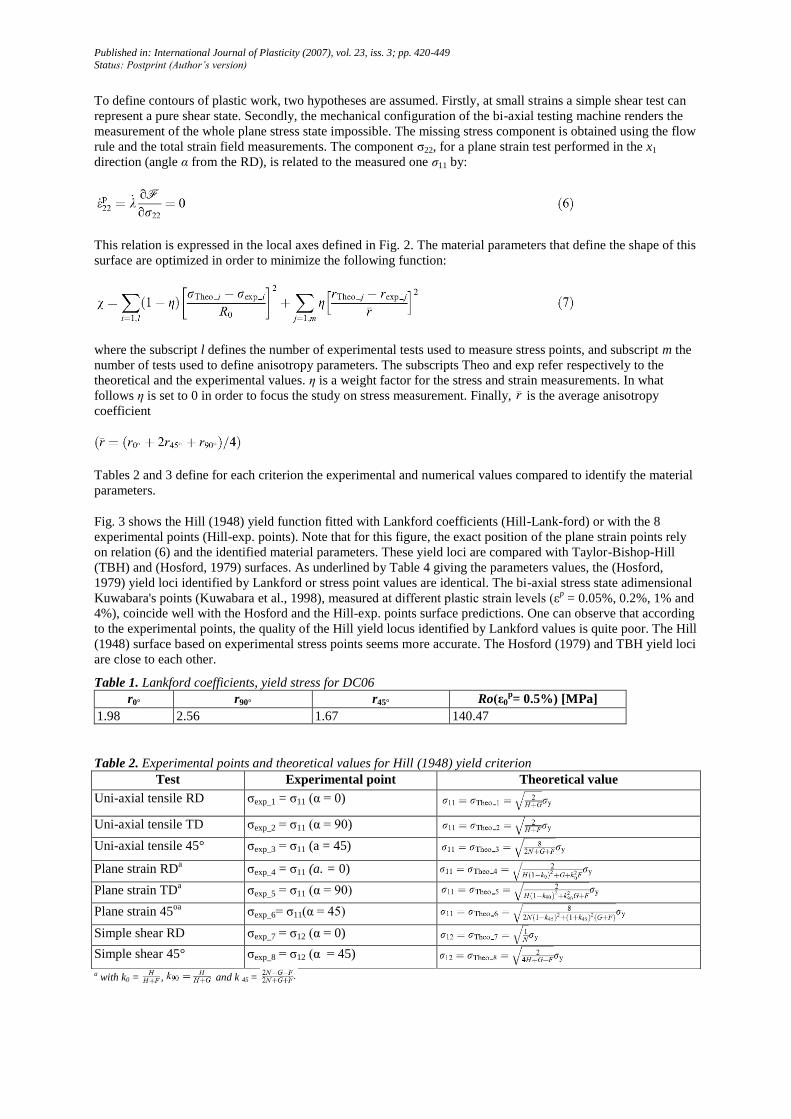
To define contours of plastic work, two hypotheses are assumed. Firstly, at small strains a simple shear test can

represent a pure shear state. Secondly, the mechanical configuration of the bi-axial testing machine renders the

measurement of the whole plane stress state impossible. The missing stress component is obtained using the flow

rule and the total strain field measurements. The component ζ22, for a plane strain test performed in the x1

direction (angle α from the RD), is related to the measured one σ11 by:

This relation is expressed in the local axes defined in Fig. 2. The material parameters that define the shape of this

surface are optimized in order to minimize the following function:

where the subscript l defines the number of experimental tests used to measure stress points, and subscript m the

number of tests used to define anisotropy parameters. The subscripts Theo and exp refer respectively to the

theoretical and the experimental values. η is a weight factor for the stress and strain measurements. In what

follows η is set to 0 in order to focus the study on stress measurement. Finally, is the average anisotropy

coefficient

Tables 2 and 3 define for each criterion the experimental and numerical values compared to identify the material

parameters.

Fig. 3 shows the Hill (1948) yield function fitted with Lankford coefficients (Hill-Lank-ford) or with the 8

experimental points (Hill-exp. points). Note that for this figure, the exact position of the plane strain points rely

on relation (6) and the identified material parameters. These yield loci are compared with Taylor-Bishop-Hill

(TBH) and (Hosford, 1979) surfaces. As underlined by Table 4 giving the parameters values, the (Hosford,

1979) yield loci identified by Lankford or stress point values are identical. The bi-axial stress state adimensional

Kuwabara's points (Kuwabara et al., 1998), measured at different plastic strain levels (εp = 0.05%, 0.2%, 1% and

4%), coincide well with the Hosford and the Hill-exp. points surface predictions. One can observe that according

to the experimental points, the quality of the Hill yield locus identified by Lankford values is quite poor. The Hill

(1948) surface based on experimental stress points seems more accurate. The Hosford (1979) and TBH yield loci

are close to each other.

Table 1. Lankford coefficients, yield stress for DC06

r0° r90° r45° Ro(ε0p= 0.5%) [MPa]

1.98 2.56 1.67 140.47

Table 2. Experimental points and theoretical values for Hill (1948) yield criterion

Test Experimental point Theoretical value

Uni-axial tensile RD ζexp_1 = ζ11 (α = 0)

Uni-axial tensile TD ζexp_2 = ζ11 (α = 90)

Uni-axial tensile 45° ζexp_3 = ζ11 (a = 45)

Plane strain RDa ζexp_4 = ζ11 (a. = 0)

Plane strain TD

a ζexp_5 = ζ11 (α = 90)

Plane strain 45

oa ζexp_6= ζ11(α = 45)

Simple shear RD ζexp_7 = ζ12 (α = 0)

Simple shear 45° ζexp_8 = ζ12 (α = 45)

a with k0 = , and k 45 =



Table 3. Experimental points and theoretical values for Hosford (1979) yield criterion

Test Experimental point Theoretical value

Uni-axial tensile RD ζexp_1 = ζ11 (α = 0)

Uni-axial tensile TD ζexp_2 = ζ11 (α = 90)

Plane strain RDa ζexp_3 = ζ11 (a = 0)

Plane strain TDa ζexp_4 = ζ11 (α = 90)

Simple shear 45° ζexp_5= ζ12(α = 45)

a With k0 =1/(1+ (F/H)1/(a-1) and k90 =1/(1+ (G/H)(1/a-1)).

Fig. 3. Scaled yield loci in principal stress directions in material axes X1, X2 and experimental points.

Table 4. Material parameters for DC06 steel

Yield function Identification method H F G N a

Hill (1948) Lankford coefficients 1.33 0.52 0.67 2.58 -

Hill (1948) Experimental points 1.13 0.69 0.87 2.76 -

Hosford (1979) Lankford coefficients 0.66 0.26 0.34 - 6

Hosford (1979) Experimental points 0.66 0.25 0.34 - 6

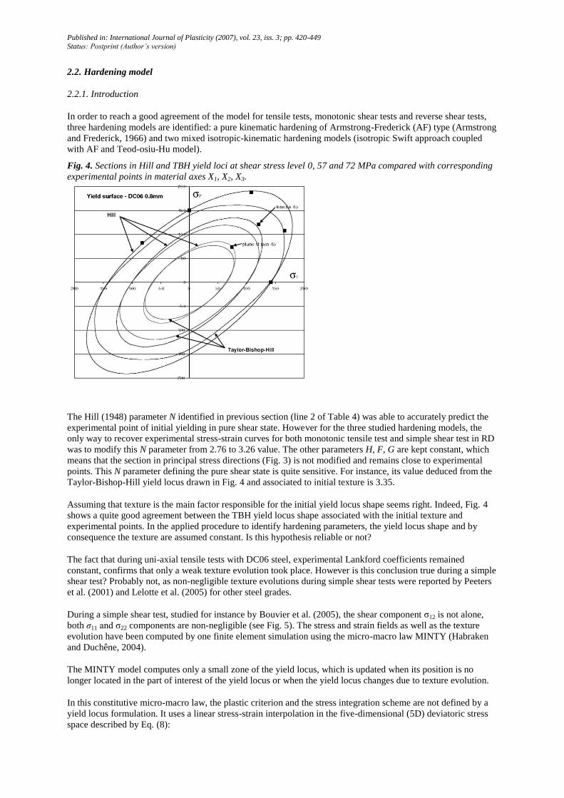
All the experimental points are plotted in Fig. 4, which shows sections of TBH and Hill exp. points yield loci at

shear stress level 0, 57 and 72 MPa. The pure shear case is 82.4 MPa in the test, when predicted values by TBH

and Hill are respectively 76.75 and 83 MPa.

These results show that mechanical tests reproducing other stress states than pure tension are required to obtain

more accurate material parameters identification.



2.2. Hardening model

2.2.1. Introduction

In order to reach a good agreement of the model for tensile tests, monotonic shear tests and reverse shear tests,

three hardening models are identified: a pure kinematic hardening of Armstrong-Frederick (AF) type (Armstrong

and Frederick, 1966) and two mixed isotropic-kinematic hardening models (isotropic Swift approach coupled

with AF and Teod-osiu-Hu model).

Fig. 4. Sections in Hill and TBH yield loci at shear stress level 0, 57 and 72 MPa compared with corresponding

experimental points in material axes X1, X2, X3.

The Hill (1948) parameter N identified in previous section (line 2 of Table 4) was able to accurately predict the

experimental point of initial yielding in pure shear state. However for the three studied hardening models, the

only way to recover experimental stress-strain curves for both monotonic tensile test and simple shear test in RD

was to modify this N parameter from 2.76 to 3.26 value. The other parameters H, F, G are kept constant, which

means that the section in principal stress directions (Fig. 3) is not modified and remains close to experimental

points. This N parameter defining the pure shear state is quite sensitive. For instance, its value deduced from the

Taylor-Bishop-Hill yield locus drawn in Fig. 4 and associated to initial texture is 3.35.

Assuming that texture is the main factor responsible for the initial yield locus shape seems right. Indeed, Fig. 4

shows a quite good agreement between the TBH yield locus shape associated with the initial texture and

experimental points. In the applied procedure to identify hardening parameters, the yield locus shape and by

consequence the texture are assumed constant. Is this hypothesis reliable or not?

The fact that during uni-axial tensile tests with DC06 steel, experimental Lankford coefficients remained

constant, confirms that only a weak texture evolution took place. However is this conclusion true during a simple

shear test? Probably not, as non-negligible texture evolutions during simple shear tests were reported by Peeters

et al. (2001) and Lelotte et al. (2005) for other steel grades.

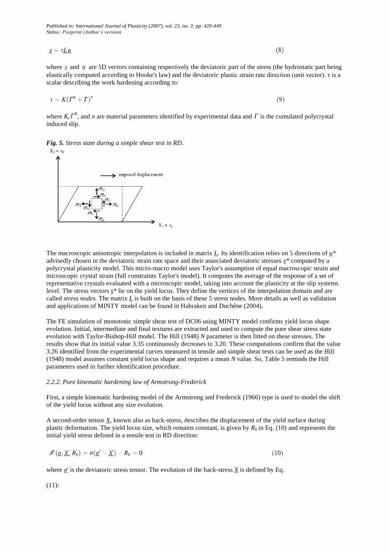
During a simple shear test, studied for instance by Bouvier et al. (2005), the shear component ζ12 is not alone,

both σ11 and ζ22 components are non-negligible (see Fig. 5). The stress and strain fields as well as the texture

evolution have been computed by one finite element simulation using the micro-macro law MINTY (Habraken

and Duchêne, 2004).

The MINTY model computes only a small zone of the yield locus, which is updated when its position is no

longer located in the part of interest of the yield locus or when the yield locus changes due to texture evolution.

In this constitutive micro-macro law, the plastic criterion and the stress integration scheme are not defined by a

yield locus formulation. It uses a linear stress-strain interpolation in the five-dimensional (5D) deviatoric stress

space described by Eq. (8):



where and are 5D vectors containing respectively the deviatoric part of the stress (the hydrostatic part being

elastically computed according to Hooke's law) and the deviatoric plastic strain rate direction (unit vector). η is a

scalar describing the work hardening according to:

where K, , and n are material parameters identified by experimental data and is the cumulated polycrystal

induced slip.

Fig. 5. Stress state during a simple shear test in RD.

The macroscopic anisotropic interpolation is included in matrix L. Its identification relies on 5 directions of u*

advisedly chosen in the deviatoric strain rate space and their associated deviatoric stresses s* computed by a

polycrystal plasticity model. This micro-macro model uses Taylor's assumption of equal macroscopic strain and

microscopic crystal strain (full constraints Taylor's model). It computes the average of the response of a set of

representative crystals evaluated with a microscopic model, taking into account the plasticity at the slip systems

level. The stress vectors s* lie on the yield locus. They define the vertices of the interpolation domain and are

called stress nodes. The matrix L is built on the basis of these 5 stress nodes. More details as well as validation

and applications of MINTY model can be found in Habraken and Duchêne (2004).

The FE simulation of monotonic simple shear test of DC06 using MINTY model confirms yield locus shape

evolution. Initial, intermediate and final textures are extracted and used to compute the pure shear stress state

evolution with Taylor-Bishop-Hill model. The Hill (1948) N parameter is then fitted on these stresses. The

results show that its initial value 3.35 continuously decreases to 3.20. These computations confirm that the value

3.26 identified from the experimental curves measured in tensile and simple shear tests can be used as the Hill

(1948) model assumes constant yield locus shape and requires a mean N value. So, Table 5 reminds the Hill

parameters used in further identification procedure.

2.2.2. Pure kinematic hardening law of Armstrong-Frederick

First, a simple kinematic hardening model of the Armstrong and Frederick (1966) type is used to model the shift

of the yield locus without any size evolution.

A second-order tensor X, known also as back-stress, describes the displacement of the yield surface during

plastic deformation. The yield locus size, which remains constant, is given by R0 in Eq. (10) and represents the

initial yield stress defined in a tensile test in RD direction:

where σ' is the deviatoric stress tensor. The evolution of the back-stress X is defined by Eq.

(11):



where Cx is the parameter describing the rate of kinematic hardening, XSAT the saturation value and is the

anisotropic equivalent plastic strain rate.

Table 5. Hill (1948) material parameters for DC06 steel

H F G N

1.13 0.69 0.87 3.26

The material parameters are fine-tuned up using an optimization method that is mainly based on Marquardt's

algorithm (Marquardt, 1963) in order to fit the stress-strain experimental curves obtained from tensile, simple

shear tests and the Bauschinger shear experiment with 10% pre-strain. The model predictions are computed by

'one finite element' simulation with the home-made FEM package Lagamine developed by the ULg team

(Habraken and Cescotto, 1990). As the number of material parameters is limited, no specific strategy is required

to identify the parameters. The set of parameters is given in Table 6.

2.2.3. Mixed hardening law (Swift + Armstrong-Frederick)

Secondly, a mixed hardening model is used. This type of hardening describes both the size and displacement

evolution of the yield surface. The constitutive equations are composed of Eqs. (12) and (13)

The material parameters are identified using the monotonic tensile test at the RD, the monotonic simple shear

test at the RD and the Bauschinger test at the RD with a 10% amount of pre-strain.

The evolution of the back-stress X is defined by Eq. (11). As the number of material parameters increases, some

care to keep physical sense of the parameters is required during the use of the optimization approach to identify

the parameters. The set of parameters is given in Table 7.

2.2.4. Mixed Teodosiu and Hu hardening law

Thirdly, a more complex mixed (isotropic-kinematic) hardening model of Teodosiu type is used (Haddadi et al.,

in press). This phenomenological model is based on microscopic and macroscopic experimental observations. It

is capable of describing monotonic large strains as well as the influence of strain-path changes and the amount of

pre-strain on the flow stress. This model uses a set of four internal variables (X, P, S, R), and 13 material

parameters are required. The back-stress X is a second-order tensor having the dimension of the stress. The

polarity P is a non-dimensional second-order tensor. A fourth-order tensor describes the directional strength of

planar persistent dislocation structures. The choice of its order is due to the need to describe the anisotropic

contribution of persistent dislocation structures to the flow stress. Finally, a scalar internal variable R, with the

dimension of the stress, takes into account the isotropic hardening caused by the statistically distributed

dislocations.

Table 6. Kinematic Armstrong-Frederick material parameters for DC06

R0 (MPa) Cx XSAT (MPa)

140.47 12.29 115.20

Table 7. Kinematic mixed material parameters for DC06

R0 (MPa) K (MPa) ε0 n m Cx XSAT (MPa)

140.47 499.9 0.0063 0.25 0.715 12.7 16.75



The yield surface is described by the following equation:

where R0 is the initial yield stress and m is the contribution of the persistent dislocation structures to the

isotropic hardening, with m [0,1]. The back-stress is ruled by the following equation:

The dependence of X on the persistent dislocation structures is included in the scalar function XSAT ( , N):

with and

The evolution of SD follows the equation:

Functions g(P,N) and h(X,N) reduce the evolution of SD upon stress reversal

and

The tensor L, associated with the latent part of the persistent dislocation structures evolves in the following

way:

with

The evolution law for the polarity tensor is:

The set of 13 material parameters present in this model is given in Table 8. The number of material parameters is

now important and some parameters are clearly dedicated only to some events (stagnation of hardening in

reverse test, in orthogonal tests,...). Details of the developed identification procedure can be found in Flores

(2006).

Figs. 6-9 compare the model predictions using the different sets of material parameters with experimental results.

For the tensile test (Fig. 6), the best fit is obtained by the mixed Teodosiu hardening. The pure kinematic

hardening model of the Armstrong-Frederick type is definitely worse. In the case of simple shear test (Fig. 6),



the best prediction is also given by the mixed Teodosiu hardening. This one is closer to experimental values than

the mixed (Swift + AF) hardening. Once again, the model of AF type is worse. Note that gamma is defined as

the tangent of the shear angle.

Fig. 7 presents Bauschinger shear test after 10% of pre-shear using the three different hardening models. One can

notice that pure AF hardening model gives bad results, it is not appropriate at all. Results are better using either a

mixed hardening or a Teodosiu one.

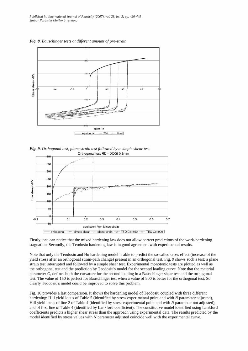
Consider now Fig. 8 which shows four Bauschinger tests at different amounts of pre-strain. These tests highlight

the presence of the Bauschinger effect, as well as the influence of the amount of pre-strain on the flow stress

stagnation when reversing the load.

Table 8. Teodosiu and Hu hardening parameters for DC06

R0

(MPa)

CR RSAT (MPa) Cx XSATO (MPa) m q CSD CSL SSAT (MPa) np nL cp

140.47 19.2 67.7 150 21.56 0.3 2.69 3.27 4.61 246.83 50 0.38 1.67

Fig. 6. Tensile test and shear test simulated by mixed hardening model (Swift + AF), pure kinematic Armstrong-

Frederick hardening, mixed Teodosiu hardening and experimental curves.

Fig. 7. Bauschinger shear test after 10% of pre-shear and simulation predictions by a mixed, a kinematic AF

and a Teodosiu hardening.



Fig. 8. Bauschinger tests at different amount of pre-strain.

Fig. 9. Orthogonal test, plane strain test followed by a simple shear test.

Firstly, one can notice that the mixed hardening law does not allow correct predictions of the work-hardening

stagnation. Secondly, the Teodosiu hardening law is in good agreement with experimental results.

Note that only the Teodosiu and Hu hardening model is able to predict the so-called cross effect (increase of the

yield stress after an orthogonal strain-path change) present in an orthogonal test. Fig. 9 shows such a test: a plane

strain test interrupted and followed by a simple shear test. Experimental monotonic tests are plotted as well as

the orthogonal test and the prediction by Teodosiu's model for the second loading curve. Note that the material

parameter Cx defines both the curvature for the second loading in a Bauschinger shear test and the orthogonal

test. The value of 150 is perfect for Bauschinger test when a value of 900 is better for the orthogonal test. So

clearly Teodosiu's model could be improved to solve this problem.

Fig. 10 provides a last comparison. It shows the hardening model of Teodosiu coupled with three different

hardening: Hill yield locus of Table 5 (identified by stress experimental point and with N parameter adjusted),

Hill yield locus of line 2 of Table 4 (identified by stress experimental point and with N parameter not adjusted),

and of first line of Table 4 (identified by Lankford coefficient). The constitutive model identified using Lankford

coefficients predicts a higher shear stress than the approach using experimental data. The results predicted by the

model identified by stress values with N parameter adjusted coincide well with the experimental curve.



Fig. 10. Tensile test and shear test simulated by mixed Teodosiu with Hill (1948) identified by Lankford

coefficient, simulated by mixed Teodosiu with Hill (1948) identified by experimental data and experimental

curves.

3. Applications

3.1. Plane strain test, validation

3.1.1. Introduction

The model identified in previous section is used to simulate a plane strain test performed on the DC06 material.

The experimental measures allow checking which model is closer to the actual material behavior.

Fig. 11 presents the specimen geometry designed for the bi-axial machine. Dimensions of the initial specimen

are 100 × 30 mm. The dotted area (30 × 3 mm) is the measurable zone. The chosen geometry allows performing

successively plane strain test and simple shear test (see Fig. 9). The deformation is imposed by the pistons

(vertical or horizontal) of the bi-axial testing machine. Here for the studied plane strain test in the RD direction,

only a vertical displacement is imposed.

The strain field can be measured in the whole deformation zone (by the optical strain gauge), and the average

stress is computed from the load cell data and the actual area. This last assumption is only valid if the stress field

is homogeneous.

The stress tensor is represented by:

with

FVertical is the load measured by the load cell and Aactual is the actual area of the specimen deduced from optical

measurement and volume conservation at the central line. The stress measured in that way will be called "global"

stress and represents the average stress over the deformation zone. The component σ22 cannot be measured with

this mechanical configuration.



Fig. 11. Specimen geometry and deformation area.

3.1.2. Experimental results

Fig. 12 shows the experimental strain field distribution at the centerline level of the sample for the respective

logarithmic strain components εIn

11 and εIn

22 at different strains.

One can notice that the strain tensor is homogeneous on the deformation area except at the free edges where

horns appear. The homogeneity depends on the amount of strain εIn

11. As the strain component εIn

22 is negligible

in the homogeneous zone of the deformation area, the expected plane strain state is actually reached. These

results are confirmed by Figs. 13 and 14 which present measured strain fields in the plane strain test respectively

for ε11 = 16% and ε11 = 20%.

Note that horns were expected according to the explanation of Fig. 15 but seem quite high (Fig. 12).

It can be explained by the initiation of a crack near the grips between ε11 = 10% and ε11 = 15%. At level ε11 =

20%, the crack is quite large and justifies the size of the horns, see Fig. 16. Such crack comes from ripping at the

grip level. Note that a notched specimen could prevent such failure but it is not used here as samples are

designed for both shear and plane strain tests.

3.1.3. Simulations results

In order to validate the parameters established in Tables 5 and 8, a finite element simulation of the plane strain

test from previous section is performed with the home-made FEM package Lagamine (Habraken and Cescotto,

1990). Table 9 summarizes the finite element simulation data. The chosen element for this simulation is an eight-

node mixed-type brick element with one integration point called BWD3D (Duchêne et al., 2005) using the new

approach to prevent volume and shear locking as well as deformation without energy (hourglass modes)

developed by Wang and Wagoner (2004).

Another important aspect in the FE code Lagamine is the method used to determine the position of the local

reference axes. These local axes are a convenient way to fulfill the objectivity of the derivatives of state variables

tensors and stress tensor. They allow modeling the anisotropic material behavior during the large rotations

involved in FE simulations.

The way to determine this local reference system is based on the Constant symmetric local velocity gradient

method developed by Munhoven and Habraken (1995). This method concerns the computation of the velocity

gradient. Usually its symmetric part is the well-known strain rate tensor and its skew-symmetric part is the spin

tensor. According to the Constant symmetric local velocity gradient method, the velocity gradient is assumed to

be constant during each FE time step. This assumption imposes the strain path. The constant value of the

velocity gradient can be determined from the configurations at the beginning of the step and the assumed

velocity field.



If it is expressed in the global reference system (which always remains fixed during the FE simulation), the so

obtained constant velocity gradient is generally non-symmetric. The symmetry of the velocity gradient can

however be obtained by expressing it in another reference system. In other words, in this method the symmetry

condition fixes the position of the local reference system. As a consequence, the spin tensor corresponding to the

symmetric constant velocity gradient is equal to zero while it is expressed in this local reference system.

Conveniently, the integration of the constitutive law in these local axes is incrementally objective without the

necessity of Jaumann type corrections. Furthermore, the local reference system is also assumed to correspond to

the material axes where material properties are defined.

Fig. 12. εIn

11 and εIn

22 components at the centerline for different levels of major strains in plane strain test

(DC06 0.8 mm thick).

Fig. 13. Major strain field for a plane strain test for a ε11 = 16%. DC06 0.8 mm.

Fig. 14. Major strain field for a plane strain test for a ε11 = 20%. DC06 0.8 mm.



Fig. 15. Evolution of ε11 strain distribution with dimensions of the sample shape.

Fig. 16. Deformed specimen for a plane strain test for a ε11 = 20%. DC06 0.8 mm.

Table 9. Finite element strategy

Finite element simulation data

Code Lagamine developed since 1984 at ArGEnCO Department

Element type BWD3D-1 integration point

Constitutive law Hill3D_KI (Hill (1948) + Teodosiu and Hu hardening law) and

MINTY law coupled with Teodosiu

Material DC06 0.8 mm thick

In order to model any heterogeneity in the test, a refined mesh of 707 elements is used.

The experimental data are then compared with the results of stress-strain curves computed with:

• the Hill (1948) surface identified by Lankford coefficients (Table 4 and Fig. 3): Hill Lankford;

• the Hill (1948) surface identified by experimental stress points at εP

0 =0.5% (Tables 4 and 5): Hill-exp. points;

• the MINTY law (with initial texture and no texture evolution during the simulation) (see Fig. 3).

Each yield locus is coupled with the Teodosiu and Hu hardening law. These three models predict similar strain

fields. All results confirm the horn strain distribution. Fig. 17(a) validates the horn level with measured strain

field while some discrepancy appears already in Fig. 17(b).

In order to be consistent with the experimental test, the stress is computed from the resulting force divided by the

actual area given in the FE simulation.

Fig. 18 compares the results. It can be seen that the constitutive model Hill-Lankford predicts a higher stress than



the other approaches. The results predicted by Hill-exp. points and MINTY are closer to experimental curve up

to a strain of 10%. Beyond this amount of strain, the crack apearing in the test justifies that curves diverge.

Fig. 17. Strain field for plane strain test (a) for a ε11 = 10%, (b) for a ε11 = 16%. DC06 0.8 mm.

Fig. 18. Plane strain test. DC06 0.8 mm.

3.2. Single point incremental forming

3.2.1. Process description

The incremental sheet forming process has emerged in the past few years as a potential alternative to

conventional sheet metal stamping processes. The process uses a smooth-ended tool under numerical control to

create a local indentation in a clamped sheet. By dragging the point of contact around the sheet according to a

programmed tool path, a wide variety of shapes may be formed without the need for specific tooling. Two

versions of the process have been explored: with and without a supporting post on the reverse side of the

workpiece. This section will only focus on the latter approach, called "single point" incremental forming (SPIF)

presented in Fig. 19.

The review paper (Jeswiet et al., 2005) summarizes some fundamental research work carried out to investigate

the deformation mechanism and material behavior. FEM simulations of this process are quite heavy as the tool

path is very long and, if no remeshing module with numerous refinement and coarsening steps is used, a refined

mesh is necessary everywhere as the tool induces very localized plastic strain.



3.2.2. Case study

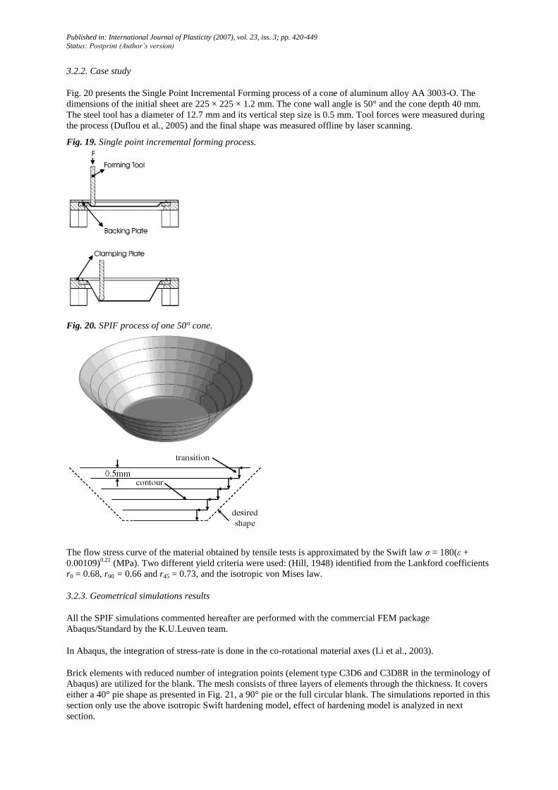
Fig. 20 presents the Single Point Incremental Forming process of a cone of aluminum alloy AA 3003-O. The

dimensions of the initial sheet are 225 × 225 × 1.2 mm. The cone wall angle is 50° and the cone depth 40 mm.

The steel tool has a diameter of 12.7 mm and its vertical step size is 0.5 mm. Tool forces were measured during

the process (Duflou et al., 2005) and the final shape was measured offline by laser scanning.

Fig. 19. Single point incremental forming process.

Fig. 20. SPIF process of one 50° cone.

The flow stress curve of the material obtained by tensile tests is approximated by the Swift law σ = 180(ε +

0.00109)0.21

(MPa). Two different yield criteria were used: (Hill, 1948) identified from the Lankford coefficients

r0 = 0.68, r90 = 0.66 and r45 = 0.73, and the isotropic von Mises law.

3.2.3. Geometrical simulations results

All the SPIF simulations commented hereafter are performed with the commercial FEM package

Abaqus/Standard by the K.U.Leuven team.

In Abaqus, the integration of stress-rate is done in the co-rotational material axes (Li et al., 2003).

Brick elements with reduced number of integration points (element type C3D6 and C3D8R in the terminology of

Abaqus) are utilized for the blank. The mesh consists of three layers of elements through the thickness. It covers

either a 40° pie shape as presented in Fig. 21, a 90° pie or the full circular blank. The simulations reported in this

section only use the above isotropic Swift hardening model, effect of hardening model is analyzed in next

section.



The results from Henrard et al. (2005), He et al. (2005a) and He et al. (2005b), confirmed by other research

teams (Fratini et al., 2004; Iseki, 2001), show that concerning the exact shape prediction at the end of the

process, the type of constitutive models is not a key factor. The discrepancy between the prediction from a 40°

pie mesh and the experiment is shown in Fig. 22. FEM simulation is accurate in the wall region but predicts a

cone bottom that is too deep compared to experimental results.

However, for the same conical shape, it has been demonstrated that using a 90° pie mesh or a full circular blank

improves the prediction. The actual process is metric and symmetry boundary conditions induce additional

stiffness that spoils the accuracy, see Fig. 23 (He et al., 2005b).

Fig. 21. Mesh used to simulate Cone SPIF process.

Fig. 22. Top surface of the cross section of the formed cone.

Fig. 23. Comparison of resulting geometries obtained with partial and full model simulations using Abaqus (at

an intermediate step; upper and lower sheet layers are plotted).

In comparison with the effect of the model geometry, the effect of the constitutive model is smaller, as shown in

Fig. 24.

3.2.4. Force analysis

Tool force measurements during the process allow another validation of the FEM simulations (He et al., 2005a).

When the mesh is sufficiently refined, the force level is not dependent on the dimensions of the piece. Models of

40°, 90° pie or full 360° circular blank using Von Mises or Hill constitutive laws with isotropic hardening have

provided nearly identical results: a prediction about 30% higher than the measurements.

To understand this difference, the strain history of one material point has been analyzed during the process in a



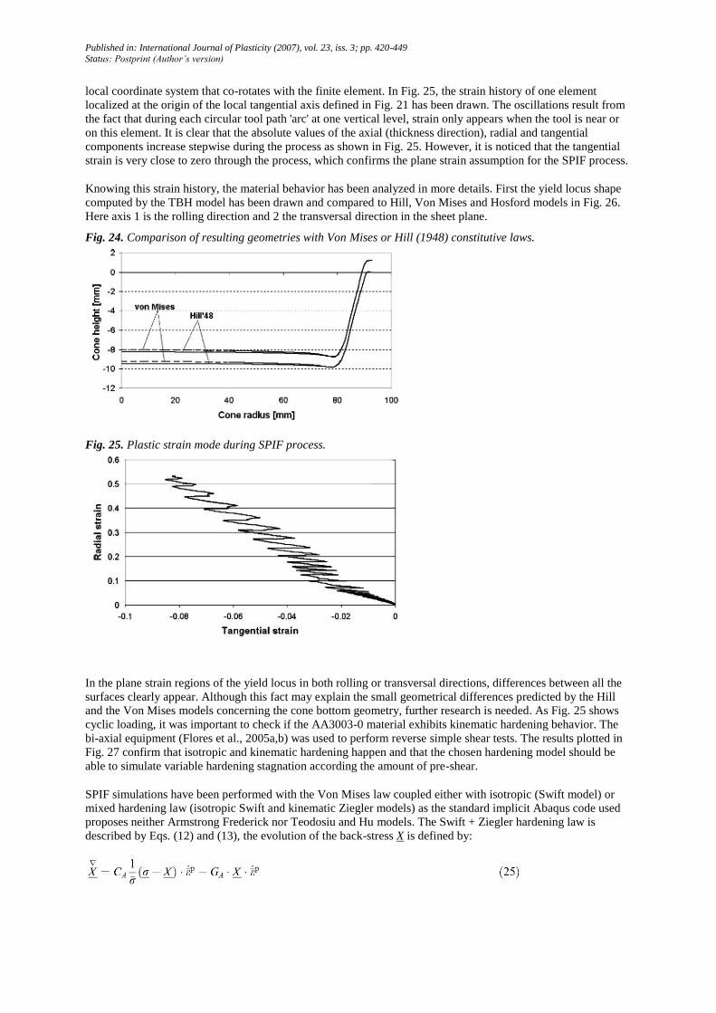
local coordinate system that co-rotates with the finite element. In Fig. 25, the strain history of one element

localized at the origin of the local tangential axis defined in Fig. 21 has been drawn. The oscillations result from

the fact that during each circular tool path 'arc' at one vertical level, strain only appears when the tool is near or

on this element. It is clear that the absolute values of the axial (thickness direction), radial and tangential

components increase stepwise during the process as shown in Fig. 25. However, it is noticed that the tangential

strain is very close to zero through the process, which confirms the plane strain assumption for the SPIF process.

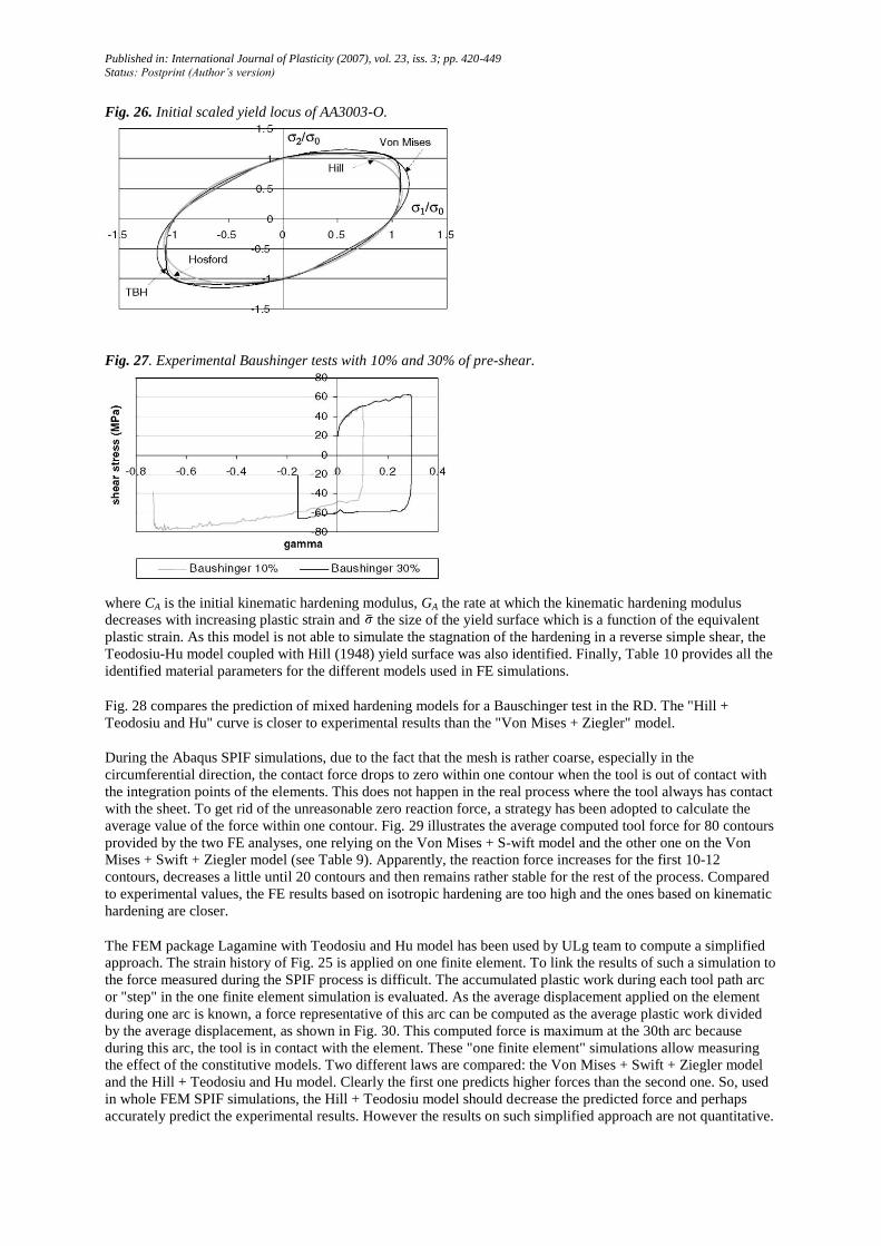
Knowing this strain history, the material behavior has been analyzed in more details. First the yield locus shape

computed by the TBH model has been drawn and compared to Hill, Von Mises and Hosford models in Fig. 26.

Here axis 1 is the rolling direction and 2 the transversal direction in the sheet plane.

Fig. 24. Comparison of resulting geometries with Von Mises or Hill (1948) constitutive laws.

Fig. 25. Plastic strain mode during SPIF process.

In the plane strain regions of the yield locus in both rolling or transversal directions, differences between all the

surfaces clearly appear. Although this fact may explain the small geometrical differences predicted by the Hill

and the Von Mises models concerning the cone bottom geometry, further research is needed. As Fig. 25 shows

cyclic loading, it was important to check if the AA3003-0 material exhibits kinematic hardening behavior. The

bi-axial equipment (Flores et al., 2005a,b) was used to perform reverse simple shear tests. The results plotted in

Fig. 27 confirm that isotropic and kinematic hardening happen and that the chosen hardening model should be

able to simulate variable hardening stagnation according the amount of pre-shear.

SPIF simulations have been performed with the Von Mises law coupled either with isotropic (Swift model) or

mixed hardening law (isotropic Swift and kinematic Ziegler models) as the standard implicit Abaqus code used

proposes neither Armstrong Frederick nor Teodosiu and Hu models. The Swift + Ziegler hardening law is

described by Eqs. (12) and (13), the evolution of the back-stress X is defined by:



Fig. 26. Initial scaled yield locus of AA3003-O.

Fig. 27. Experimental Baushinger tests with 10% and 30% of pre-shear.

where CA is the initial kinematic hardening modulus, GA the rate at which the kinematic hardening modulus

decreases with increasing plastic strain and the size of the yield surface which is a function of the equivalent

plastic strain. As this model is not able to simulate the stagnation of the hardening in a reverse simple shear, the

Teodosiu-Hu model coupled with Hill (1948) yield surface was also identified. Finally, Table 10 provides all the

identified material parameters for the different models used in FE simulations.

Fig. 28 compares the prediction of mixed hardening models for a Bauschinger test in the RD. The "Hill +

Teodosiu and Hu" curve is closer to experimental results than the "Von Mises + Ziegler" model.

During the Abaqus SPIF simulations, due to the fact that the mesh is rather coarse, especially in the

circumferential direction, the contact force drops to zero within one contour when the tool is out of contact with

the integration points of the elements. This does not happen in the real process where the tool always has contact

with the sheet. To get rid of the unreasonable zero reaction force, a strategy has been adopted to calculate the

average value of the force within one contour. Fig. 29 illustrates the average computed tool force for 80 contours

provided by the two FE analyses, one relying on the Von Mises + S-wift model and the other one on the Von

Mises + Swift + Ziegler model (see Table 9). Apparently, the reaction force increases for the first 10-12

contours, decreases a little until 20 contours and then remains rather stable for the rest of the process. Compared

to experimental values, the FE results based on isotropic hardening are too high and the ones based on kinematic

hardening are closer.

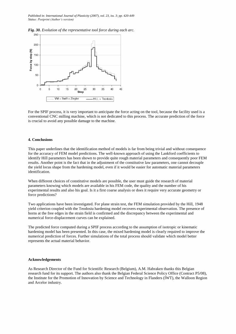
The FEM package Lagamine with Teodosiu and Hu model has been used by ULg team to compute a simplified

approach. The strain history of Fig. 25 is applied on one finite element. To link the results of such a simulation to

the force measured during the SPIF process is difficult. The accumulated plastic work during each tool path arc

or "step" in the one finite element simulation is evaluated. As the average displacement applied on the element

during one arc is known, a force representative of this arc can be computed as the average plastic work divided

by the average displacement, as shown in Fig. 30. This computed force is maximum at the 30th arc because

during this arc, the tool is in contact with the element. These "one finite element" simulations allow measuring

the effect of the constitutive models. Two different laws are compared: the Von Mises + Swift + Ziegler model

and the Hill + Teodosiu and Hu model. Clearly the first one predicts higher forces than the second one. So, used

in whole FEM SPIF simulations, the Hill + Teodosiu model should decrease the predicted force and perhaps

accurately predict the experimental results. However the results on such simplified approach are not quantitative.



So the FEM SPIF simulations must confirm the accuracy of this last model. The only conclusion is the non-

negligible effect of the chosen mixed hardening model.

Table 10. Material parameters for AA3003-O for three different models

Von Mises + Isotropic Swift hardening

K (MPa) εo n m

180.0 0.00109 0.21 1

Von Mises + mixed hardening (Swift + Ziegler)

K (MPa) εo n m CA GA

146.7 0.001496 0.229 1 240.6 11.2

Hill (1948) material parameters

F G H N

1.224 1.194 0.806 3.92

Hill (1948) + mixed hardening (Teodosiu-Hu)

R0 CR RSAT Cx XSAT0 m q CSD CsL SSAT np nL cp

43 73.3 25.22 300.2 8.45 0.399 1 6.94 0 70.67 130.92 1 0.97

Fig. 28. Experimental results ad numerical predictions for a Bauschinger test with 10% of pre-shear.

Fig. 29. Force measurements during SPIF process and Abaqus predictions.



Fig. 30. Evolution of the representative tool force during each arc.

For the SPIF process, it is very important to anticipate the force acting on the tool, because the facility used is a

conventional CNC milling machine, which is not dedicated to this process. The accurate prediction of the force

is crucial to avoid any possible damage to the machine.

4. Conclusions

This paper underlines that the identification method of models is far from being trivial and without consequence

for the accuracy of FEM model predictions. The well-known approach of using the Lankford coefficients to

identify Hill parameters has been shown to provide quite rough material parameters and consequently poor FEM

results. Another point is the fact that in the adjustment of the constitutive law parameters, one cannot decouple

the yield locus shape from the hardening model, even if it would be easier for automatic material parameters

identification.

When different choices of constitutive models are possible, the user must guide the research of material

parameters knowing which models are available in his FEM code, the quality and the number of his

experimental results and also his goal. Is it a first coarse analysis or does it require very accurate geometry or

force predictions?

Two applications have been investigated. For plane strain test, the FEM simulation provided by the Hill, 1948

yield criterion coupled with the Teodosiu hardening model recovers experimental observation. The presence of

horns at the free edges in the strain field is confirmed and the discrepancy between the experimental and

numerical force-displacement curves can be explained.

The predicted force computed during a SPIF process according to the assumption of isotropic or kinematic

hardening model has been presented. In this case, the mixed hardening model is clearly required to improve the

numerical prediction of forces. Further simulations of the total process should validate which model better

represents the actual material behavior.

Acknowledgements

As Research Director of the Fund for Scientific Research (Belgium), A.M. Habraken thanks this Belgian

research fund for its support. The authors also thank the Belgian Federal Science Policy Office (Contract P5/08),

the Institute for the Promotion of Innovation by Science and Technology in Flanders (IWT), the Walloon Region

and Arcelor industry.



References

Armstrong, P.J., Frederick, C.O., 1966. A mathematical representation of the multiaxial Bauschinger effect. GEGB Report RD/B/N731,

Berkeley Nuclear Laboratories.

Banabic, B., Bunge, H.-J., Pδhlandt, K., Tekkaya, A.E., 2000. Formability of Metallic Materials. Springer, pp. 139-140.

Bouvier, S., Teodosiu, C., Haddadi, H., Tabacaru, V., 2003. Anisotropic work-hardening behaviour of structural steels and aluminium alloys

at large strains. Journal de Physique IV 105, 215-222.

Bouvier, S., Haddadi, H., Levée, P., Teodosiu, C., 2005. Simple shear test: experimental techniques and characterizations of the plastic anisotropy of rolled sheets at large strains. Journal of Material Processing Technology 172 (1), 96-103.

Brunet, M., Morestin, F., Godereaux, S., 2001. Nonlinear kinematic hardening identification for anisotropic sheet metals with bending-

unbending tests. Journal of Engineering Materials and Technology 123, 378-383.

Duchêne, L., de Montleau, P., El Houdaigui, F., Bouvier, S., Habraken, A.M., 2005. Analysis of texture evolution and hardening behavior

during deep drawing with an improved mixed type FEM element. In: Smith, L.M., Pourboghrat, F., Yoon, J.-W., Stoughton, T.B. (Eds.),

Proc. of the 6th Inter. Conf. and Workshop on Numerical Simulation of 3D Sheet Metal Forming Processes, On the Cutting Edge of

Technology NUMISHEET, Detroit, MI, USA. AIP 778, 409-414.

Duflou, J.R., Szekeres, A., Vanherck, P., 2005. Force measurements for single point incremental forming: an experimental study. Advanced Materials Research 6-8, 441-448.

Flores, P., 2006, Development of experimental equipment and identification procedures for sheet metal constitutive laws. Ph.D. thesis, ULG,

Liège.

Flores, P., Rondia, E., Habraken, A.M., 2005a. Development of an experimental equipment for the identification of constitutive laws (Special

Issue). International Journal of Forming Processes 117-137.

Flores, P., Moureaux, P., Habraken, A.M., 2005b. Material identification using a bi-axial test machine. Advances in Experimental Mechanics IV 3-4, 91-97.

Fratini, L., Ambrogio, G., Di Lorenzo, R., Filice, L., Micari, F., 2004. Influence of mechanical properties of the sheet material on formability

in single point incremental forming. CIRP Annals 53 (1), 207-210.

Habraken, A.M., Cescotto, S., 1990. An automatic remeshing technique for finite element simulation of forming processes. International

Journal Numerical Methods in Engineering (30/8), 1503-1525.

Habraken, A.M., Duchêne, L., 2004. Anisotropic elasto-plastic finite element analysis using a stress-strain interpolation method based on a polycrystalline model. International Journal of Plasticity 20, 1525-1560.

Haddadi, H., Bouvier, S., Banu, M., Maier, C., Teodosiu, C., 2006. Towards an accurate description of the anisotropic behaviour of sheet

metals under large plastic deformations: modelling, numerical analysis and identification. International Journal of Plasticity 22 (12), 2226-2271.

He, S., Van Bael, A., Van Houtte, P., Szekeres, A., Duflou, J.R., Henrard, C., Habraken, A.M., 2005a. Finite element modeling of

incremental forming of aluminium sheets. Advanced Materials Research 6-8, 525-532.

He, S., Van Bael, A., Van Houtte, P., Tunckol, Y., Duflou, J., Henrard, C., Bouffioux, C., Habraken, A.M., 2005b. Effect of FEM choices in

the modelling of incremental forming of aluminium sheets. In: Banabic, D. (Ed.), Proceedings of the 8th ESAFORM Conference on Material

Forming. The Publishing House of the Romanian Academy, pp. 711-714.

Henrard, C., Habraken, A.M., Szekeres, A., Duflou, J.R., He, S., Van Bael, A., Van Houtte, P., 2005. Comparison of FEM simulations for

the incremental forming process. Advanced Materials Research 6-8, 533-542.

Hill, R., 1948. A theory of the yielding and plastic flow of anisotropic materials. Proceedings of the Royal Society of London A 193, 281-297.

Hosford, W.F., 1979. On yield loci of anisotropic cubic metals. In: Proceedings of the 7th North American Metalworking Conf. (NMRC),

SME, Dearborn, MI, pp. 191-197.

Hosford, W.F., 1998. Reflections on the Dependence of Plastic Anisotropy on Texture. Materials Science and Engineering A 257, 1-8.

Hu, W., 2005. An orthotropic yield criterion in a 3-D general stress state. International Journal of Plasticity 21, 1771-1796. Iseki, H., 2001.

An approximate deformation analysis and FEM analysis for the incremental bulging of sheet metal using a spherical roller. Journal of Materials Processing Technology 111, 150-154.

Jeswiet, J., Micari, F., Hirt, G., Bramley, A., Duflou, J., Allwood, J., 2005. Asymmetric single point incremental forming of sheet metal.



CIRP Annals, 54/2.

Kuwabara, T., Ikeda, S., Kuroda, K., 1998. Measurement and analysis of differential work hardening in cold-rolled steel sheet under bi-axial

tension. Journal of Material Processing Technology 80-81, 517-523.

Lelotte, T., Gerday, A.F., Flores, P., Bouvier, S., Van Houtte, P., Habraken, A.M., 2005. Axes rotation during simple shear test:

measurement and predictions. In: VIII Int. Conf. on Comp. Plasticity (COMPLAS VIII), Barcelona, Spain, pp. 1027-1030.

Li, S., Hoferlin, E., Van Bael, A., Van Houtte, P., Teodosiu, C, 2003. Finite element modeling of plastic anisotropy induced by texture and strain-path change. International Journal of Plasticity 19, 647-674.

Marquardt, D.W., 1963. An algorithm for least-squares estimation of non-linear parameters. Journal of the Society for Industrial and Applied

Mathematics 11, 431-440.

Munhoven, S., Habraken, A.M., 1995. Application of an anisotropic yield locus based on texture to a deep, simulation of materials

processing: theory, methods and applications. In: Shen, Dawson (Eds.), © 1995

Balkema, Rotterdam, pp. 767-772. ISBN 90 5410 553 4. Peeters, B., Hoferlin, E., Van Houtte, P., Aernoudt, E., 2001. Assessment of crystal plasticity based calculation of lattice spin of polycrystalline metals for FE implementation. International Journal of Plasticity 17, 819- 836.

Stoughton, T.B., Yoon, J.W., 2006. Review of Drucker's postulate and the issue of plastic stability in metal forming. International Journal of

Plasticity 22, 391-433.

Teodosiu, C., Hu, Z., 1995. Evolution of the intragranular microstructure at moderate and large strains: modelling and computational

significance. In: Shen, Dawson (Eds.), Simulation of Material Processing: Theory, Methods and Applications, © 1995 Balkema, Rotterdam,

pp. 173-182. ISBN 90 5410 553 4.

Teodosiu, C., Hu, Z., 1998. Microstructure in the continuum modelling of plastic anisotropy. In: Carstensen, J.V., Leffers, T., Lorentzen, T.,

Pedersen, O.B., Sorensen, B.F., Winther, G. (Eds.), Proceedings of the 19th Riso International Symposium on Materials Science: Modelling

of Structure and Mechanics of Materials from Microscale to Product. Riso National Laboratory, Roskilde, Denmark, pp. 149-168.

Tong, W., 2006. A plane stress anisotropic plastic flow theory for orthotropic sheet metals. International Journal of Plasticity 22, 497-535.

Van Houtte, P., 1988. A comprehensive mathematical formulation of an extended Taylor-Bishop-Hill model featuring relaxed constraints,

the Renouard-Wintenberger theory and a strain rate sensitivity model. Textures and Microstructures 8-9, 313-350.

Van Houtte, P., 2002. ODFLAM Software. Part of the latest version of MTM-FHM Software System, Katholieke Universiteit Leuven.

Wang, J., Wagoner, R.H., 2004. A new hexahedral solid element for 3D FEM simulation of sheet metal forming. In: Proceedings of the 8th

Numiform Conference, vol. 712 (1), pp. 2181-2186.

Yoon, J.W., Barlat, F., Dick, R.E., Karabin, M.E., 2006. Prediction of six or eight ears in a drawn cup based on a new anisotropic yield

function. International Journal of Plasticity 22, 174-193.

Documents

Model identification and FE simulations: Effect of ... · In practice, different metal forming processes such as deep drawing, stamping or bending are required to ... associated plasticity