MODEL-FREE EVALUATION OF DIRECTIONAL ......foreign exchange markets using a model-free econometric procedure. In this paper, we examine In this paper, we examine Ł Correspondence

JOURNAL OF APPLIED ECONOMETRICSJ. Appl. Econ. 22: 855–889 (2007)Published online in Wiley InterScience(www.interscience.wiley.com) DOI: 10.1002/jae.965

MODEL-FREE EVALUATION OF DIRECTIONALPREDICTABILITY IN FOREIGN EXCHANGE MARKETS

JAEHUN CHUNGa AND YONGMIAO HONGb*a Balance Sheet Measurement, Canadian Imperial Bank of Commerce, Toronto, Ontario, Canada

b Department of Economics, Cornell University, Ithaca, New York, USA; Wang Yanan Institute for Studies in Economics,Xiamen, China

SUMMARYWe examine directional predictability in foreign exchange markets using a model-free statistical evaluationprocedure. Based on a sample of foreign exchange spot rates and futures prices in six major currencies, wedocument strong evidence that the directions of foreign exchange returns are predictable not only by the pasthistory of foreign exchange returns, but also the past history of interest rate differentials, suggesting that thelatter can be a useful predictor of the directions of future foreign exchange rates. This evidence becomesstronger when the direction of larger changes is considered. We further document that despite the weakconditional mean dynamics of foreign exchange returns, directional predictability can be explained by strongdependence derived from higher-order conditional moments such as the volatility, skewness and kurtosisof past foreign exchange returns. Moreover, the conditional mean dynamics of interest rate differentialscontributes significantly to directional predictability. We also examine the co-movements between two foreignexchange rates, particularly the co-movements of joint large changes. There exists strong evidence that thedirections of joint changes are predictable using past foreign exchange returns and interest rate differentials.Furthermore, both individual currency returns and interest rate differentials are also useful in predictingthe directions of joint changes. Several sources can explain this directional predictability of joint changes,including the level and volatility of underlying currency returns. Copyright 2007 John Wiley & Sons, Ltd.

Received 6 December 2005; Revised 14 August 2006

1. INTRODUCTION

Since the seminal work of Meese and Rogoff (1983a), the efficiency of foreign exchange marketshas been examined extensively. While market efficiency is an ongoing argument, it is widelyviewed that it is difficult to beat the martingale model or the random walk model in predictingthe conditional mean dynamics of foreign exchange rate changes (e.g., Diebold and Nason, 1990;Hsieh, 1988, 1989, 1993; McCurdy and Morgan, 1987; Meese and Rogoff, 1983a, 1983b; Meeseand Rose, 1991). Most existing studies, however, are based on the tests of some forecast models orforecast rules. In other words, these studies examine the efficiency of models rather than data, andas a result their conclusions were model dependent. In addition, as Taylor (1995) has reported, sucha model-driven test for the foreign exchange market efficiency seems elusive with the presence ofrisk premia and expectation errors. Therefore, it is highly desirable to evaluate the efficiency offoreign exchange markets using a model-free econometric procedure. In this paper, we examine

Ł Correspondence to: Yongmiao Hong, Department of Economics, Cornell University, 424 Uris Hall, Ithaca, NY14850, USA. E-mail: [email protected]/grant sponsor: Cheung Kong Scholarship of the Chinese Ministry of Education and Xiamen University.Contract/grant sponsor: National Science Foundation; Contract/grant number: SES-0111769.

Copyright 2007 John Wiley & Sons, Ltd.

856 J. CHUNG AND Y. HONG

directional predictability in foreign exchange markets using a class of new model-free evaluationprocedures.

There are several reasons why the directional predictability of foreign exchange returns isimportant. First, from a statistical point of view, it may be relatively easier to predict the directionof changes. Directional predictability depends on all conditional moments rather than merely theconditional mean of the foreign exchange rate changes (Christoffersen and Diebold, 2002; Hongand Chung, 2006). Thus, the forecasts of the direction of changes may be easier than the forecasts ofthe conditional mean. Cheung et al. (2005) have shown that certain structural models outperformthe random walk with statistical significance in foreign exchange markets when evaluated ondirection-of-change criteria, although they are less able to forecast the conditional mean dynamicsof the foreign exchange rate changes (see also Breen et al., 1989; Engel 1994; Kuan and Liu, 1995;Larsen and Wozniak, 1995; Leitch and Tanner, 1991, 1995; Pesaran and Timmermann, 1995, 2002;Shephard and Rydberg, 2003; Satchell and Timmermann, 1995; for more related discussions).

Second, from an economic point of view, the directional predictability of foreign exchangereturns is more relevant to many financial applications than forecasting the conditional meandynamics. For example, Leitch and Tanner (1991, 1995) showed that the direction-of-changecriterion may be better able to capture a utility-based measure of forecasting performance suchas economic profits (see Granger and Pesaran, 2000; Pesaran and Skouras, 2001; for furtherdiscussion). Market timing, one form of active asset allocation management, is essentiallythe prediction of turning points in financial markets. There have been a number of tests formarket timing ability in the literature (e.g., Henriksson and Merton, 1981; Cumby and Modest,1987; Pesaran and Timmermann, 1992), although they are intended to evaluate the directionalpredictability of models or forecasters.

Third, the direction of changes is an important maneuver in foreign exchange rate markets. Forinstance, the technical trading rules widely used by foreign exchange dealers (Taylor and Allen,1992) are heavily based on forecasts of direction of changes (e.g., Pring, 1991). Also, centralbanks under pegged exchange rate systems often use the direction of exchange rate changes as akey instrument to maintain monetary stability. They will intervene in the foreign exchange marketwhen the domestic currency is expected either to appreciate or depreciate beyond a certain, oftenpolitically determined threshold. Hence the study on the direction of changes will provide importantinsights to market practitioners and policy makers.

Finally, the direction of changes can be an alternative instrument for the link between foreignexchange rates and interest rates. Most early studies on this subject have focused on the relationshipbetween the level of (expected) exchange rate changes and interest rate differentials, formallyknown as ‘uncovered interest rate parity (UIP)’. Unfortunately, while the theoretical implication ofthe UIP–interest rate differentials serve as a useful predictor of the future spot foreign exchangerates is important, its validity has been questioned on various grounds in the literature. Thismotivates us to look for an alternative relationship, that is, whether interest rate differentials areuseful to predict the direction of future foreign exchange rates. This still links foreign exchangerates with interest rates, but relaxes a rather restrictive condition imposed by UIP, under which theexpected changes in a foreign exchange rate should exactly counterbalance the difference betweendomestic and foreign interest rates.

One interesting issue in the foreign exchange markets is currency crisis. There have been avariety of theoretical and empirical studies on currency crisis (see Kaminsky et al., 1998, for anexcellent survey). Due to quantifying difficulties, a currency crisis is typically represented by anindicator (binary) function, which is equal to unity if there is a sudden fall of foreign exchange

Copyright 2007 John Wiley & Sons, Ltd. J. Appl. Econ. 22: 855–889 (2007)DOI: 10.1002/jae

DIRECTIONAL PREDICTABILITY IN EXCHANGE RATES 857

rate beyond a certain threshold, namely, a large negative change. Several recent studies furthersuggest that some models for binary dependent variables (i.e., the currency crisis indicator) mayhave descriptive or predictive ability for future currency crises (e.g., Frankel and Rose, 1996a;Berg and Pattillo, 1999; Kumar et al., 2003). Perhaps even more interesting is when a currencycrisis spreads from one market to another (or they occur simultaneously), which is commonlyreferred to as ‘market contagion’. This growing and pervasive phenomenon suggests that duringa crisis period a large adverse price change in one market will be closely followed by a largeadverse price change in another market, regardless of market fundamentals (King and Wadhwani,1990), implying a quite strong positive directional dependence between two markets during theturmoil period.1 In pursuit of better understanding of directional movement, it is useful to examinethe directions of large changes and large joint changes.

Ultimately, it is an empirical issue whether the direction of foreign exchange rate changes ispredictable. All technical trading rules are built on a fundamental assumption; i.e., the pattern of theforeign exchange market is regular and can be repeated. Indeed, technically oriented forecasts aregenerally more accurate in predicting the direction of changes in the exchange rates than economicstructural models (e.g., Cumby and Modest, 1987; Somanath, 1986). Considerable evidence inthe literature suggests that these rules may generate significant profits in the foreign exchangemarket. Examples include Dooley and Shaffer (1983), Sweeney (1986), and Levich and Thomas(1993) for the use of filter rules, Lee and Mathur (1996) and LeBaron (1999) for the use ofmoving average trading rules, and Neely and Weller (1999) for the use of genetic programming.Some speculations suggest that the directions of foreign exchange rate changes are predictableby anticipating monetary policies: the monetary authorities might use foreign exchange marketintervention as a means of monetary policies (rather than merely as an instrument for exchange ratesstability) to achieve and strengthen major macroeconomic goals, such as high employment, lowinflation, economic growth, trade balance, and price stability. In fact, several studies suggest that themonetary authorities may actually intervene to signal future monetary policies (e.g., Carlson et al.,1995; Mussa, 1981). Thus, once the speculators realize the expected future stance of monetarypolicies, they are able to exploit potential gains from the aforementioned intervention by correctlyfollowing the direction of the short-run trend (e.g., Baillie and Osterberg, 1997; Bonser-Neal andTanner, 1996; Dominguez and Frankel, 1993; Ghosh, 1992).

There is a growing consensus that real and nominal exchange rates exhibit mean reversion towardthe equilibrium level implied by economic fundamentals (e.g., Abuaf and Jorion, 1990; Frankeland Rose, 1996b; Jorion and Sweeney, 1996; Lothian and Taylor, 1996).2 More interestingly,the degree of mean reversion is stronger when the deviation of actual exchange rates from theequilibrium is greater (e.g., Taylor and Peel, 2000; Taylor et al., 2002). The role of transactioncosts has been central to theoretical models of explaining this nonlinearity. For instance, Dumas(1992) and Sercu et al. (1995) suggest that transaction costs produce ‘a band of inaction’ withinwhich international price differentials incur no arbitrage. Similarly, due to friction and politicalcosts, it is natural to expect greater intensity of market intervention when a substantial deviationis observed and expected to continue (Ito and Yabu, 2004). Consequently, the adjustment process

1 See, for example, Bae et al. (2003) for further discussion.2 The commonly used benchmark is the level implied by the Purchasing Power Parity. In its relative version, this propositionstates that the percentage change in nominal exchange rates should be equal to the inflation differentials (See Bleaneyand Mizen, 1995, for a survey).



takes place only when the perceived misalignment is large enough to cover such costs.3 Analternative viewpoint can be discerned from the exchange rate behavior postulated by the targetzone model (Krugman, 1991). In an exchange rate target zone, the monetary authorities allowexchange rates to float freely within the zone. However, if the rates approach the edge, i.e., upper orlower limits of the zone, they actively intervene in the foreign exchange market. In this framework,the exchange rates follow a bounded process and thereby exhibit mean reversion within the zone(see Anthony and MacDonald, 1998, 1999, for empirical evidence of this implication). Again,these findings may provide another strand of evidence that supports directional predictabilityin foreign exchange markets. In the presence of (nonlinear) mean reversion of exchange rates,it is intuitively plausible that the direction of foreign exchange rate changes is predictable frommonetary fundamentals. That is, when the domestic interest rate is significantly higher than foreigninterest rates or when the domestic inflation rate is significantly lower than foreign inflation rates,appreciation of the domestic currency is anticipated because of exogenous realignment pressures(i.e., market intervention) or endogenous realignment pressures (i.e., market forces to bring therates back to the equilibrium), which are inherited by a mean reversion process. Therefore, we areat least able to predict the direction of future foreign exchange rate changes, even if it is difficultto predict the level of the exchange rate changes using economic fundamentals.

As pointed out earlier, the preceding studies described are model specific. They providedirectional predictability of models (rather than data), but cannot explain why there exists such anopportunity to profit in the foreign exchange market from the currency attacks or technical tradingrules. In contrast, our model-free evaluation will provide a statistical explanation based upon rawobserved data about whether the direction of changes is predictable. In addition, it provides someguidance in constructing forecast models, such as the choice of information sets and conditionalvariables.

Based on a sample of spot rates and futures prices in six major currencies, our analysis revealsa number of interesting findings. First, we find significant evidence on directional predictabilityfor the majority of both spot and future foreign exchange rates. The directions of foreign exchangereturns can be predicted not only by the past history of foreign exchange returns, but also by thepast history of interest rate differentials. Directional predictability for larger returns is stronger,owing to the persistent volatility clustering of past foreign exchange rate changes and the time-varying conditional mean dynamics of interest rate differentials. We also find significant evidenceon directional predictability of the co-movement between two foreign exchange rates, especiallythe co-movement of large changes. These results are useful for financial risk management andinvestment diversification, as they provide useful information for understanding extreme marketmovements and extreme market co-movements.

Our findings have important implications. First, the evidence of directional predictabilityprovides a solid statistical basis for any successful directional forecast models and technicaltrading rules. Second, our results suggest that interest rate differentials can be useful instrumentsin predicting the direction of foreign exchange rate changes. Third, the documented dependenciesbetween the direction of foreign exchange rate changes and two conditioning series—the pastexchange rate changes and past interest rate differentials—suggest that both foreign exchangemarket intervention and interest rate defense can be effective tools in managing foreign exchange

3 See Kilian and Taylor (2001), Taylor et al. (2002) and Taylor and Taylor (2004) for further discussion and other possiblesources of this asymmetry.



markets. Lastly, our evidence of directional predictability of joint changes in two currenciessuggests that it is possible to predict simultaneous foreign exchange markets movements.

The paper is organized as follows: Section 2 discusses hypotheses on directional predictability inforeign exchange rate changes, including those large changes and the direction of co-movements intwo currencies. Section 3 describes the model-free evaluation methods for directional predictability.Section 4 describes the data and summary statistics, Section 5 presents our empirical findings anddiscusses their implications, and Section 6 contains concluding remarks and directions for futureresearch.

2. DIRECTIONAL PREDICTABILITY IN FOREIGN EXCHANGE MARKETS

Let Yt denote the return of the spot foreign exchange rate St at time t. We define a directionindicator function

Zt�c� D 1�Yt > c� �1�

where 1�Ð� denotes the indicator function, taking value 1 when Yt > c and value zero when Yt � c,and c is a threshold constant. This indicator function characterizes the direction of positive pricechanges. A similar indicator function can be defined for the direction of negative price changeswhen Yt < �c.

It is important to consider directional predictability of the foreign exchange rate with differentthreshold values for the following reasons. First, since an asset price may be quoted in minimumprice increments (or ticks), marginal investors who determine market prices may be more interestedin whether the asset prices rise above or fall below such thresholds. In a similar vein, those investorswho are in pursuit of profit may be further interested in the direction of the changes large enough toensure net profits after transaction costs. Therefore, the provision of a threshold value can be seenas representing practical considerations to help build more successful trading strategies. Next, thederiving forces of small and large changes in asset prices may be different. Maheu and McCurdy(2003), for example, show that the dynamics of returns can consist of two different components:(i) occasional jumps (i.e., large changes),4 which are driven by important news events, and tend tobe clustered together; (ii) (smooth) small changes, which are due to liquidity trading or strategictrading, as information dissimilates over time. At the same time, it has been observed that there isan asymmetry in the dependence structure for small and large changes, as in Longin and Solnik(2001), Ang and Chen (2002), and Hong et al. (2007), who found the correlation is strongerbetween large changes than that between small changes, and even stronger on the downside (i.e.,negative large returns). Lastly, investors may have different valuation assessments between smalland large changes in the foreign exchange rates. For example, momentum traders, who seekto exploit a short-term trend, may react more strongly to large changes since the direction andstrength of the trend become more recognizable at the larger changes. In addition, large changesoften contain more valuable information, while small changes display mere noise. Therefore, it isnecessary for investors to segment price changes so as to filter out irrelevant information from theobservations.5

4 Jorion (1988) points out that there are more jumps in the foreign exchange market than in stock markets.5 This is exactly the rationale behind the most popular technical trading rule—filter rules. Filter rules generate a ‘buy’signal when a currency rises c% above its most recent trough; a ‘sell (short)’ signal when it falls by c% from the recentpeak. Smaller filters capture turning points better but lead to more frequent trades and higher transaction costs. In contrast,larger filters result in less frequent trades and lower brokerage fees, but they miss the turning points by a larger amount.



In practice, the choice of threshold c can either be made conditional on data or held fixed atmultiple values such as tick sizes or transaction costs. There is no obvious rationale for preferringone or another criterion: a posterior threshold gained from the observations may be more suitablefor the purpose of statistical data analysis, while the latter will be of interest to those in pursuitof practical use. Since our study concerns a statistical evaluation of directional predictability, wewill use the multiples of the standard deviation �Y D p

var�Yt� without loss of generality.6

We are interested in testing whether the direction of foreign exchange rate changes with thresholdc is predictable using the history of its own past changes. The null hypothesis is

�0 : E[Zt�c�jIt�1] D E[Zt�c�] almost surely �a.s.� �2�

where It�1 � fYt�1, Yt�2, . . .g is the information set available at time t � 1. Note that our nullhypothesis �0 is not the same as the hypothesis of E�YtjIt�1� D � a.s. for some constant �, wherethe latter hypothesis checks whether there exists a predictable time-varying conditional mean. Itis shown that, irrespective of the existence of a time-varying conditional mean predictability,directional predictability may exist through the interaction between a nonzero unconditional mean�, volatility dependence, and serial dependence in higher-order conditional moments such asskewness and kurtosis (Christoffersen and Diebold, 2002; Hong and Chung, 2006). This fact, thatdirectional predictability can be derived from such various sources, may explain why it is easierto predict the direction than the level of the change, as many empirical studies document.

While rejecting the null hypothesis �0 of no directional predictability is evidence against marketefficiency, it could be viewed as an alternative way to assess the efficacy of successful exchangemarket intervention.7 Note that, under the null hypothesis �0 of (2), market intervention througha sale/purchase of the foreign (or domestic) currency, has no impact on the direction of exchangerates movements. In other words, for intervention to be effective, it should be able to systematicallyaffect the direction of foreign exchange rates. Since the sequence of direction indicators fZt�c�gis a Bernoulli process, we have only two possible outcomes: ‘up’ or ‘down’. Thus, the outcomesfollowing the intervention identified as either ‘success’ or ‘failure’ might be drawn randomlyrather than resulting from the intended effects of the intervention (see, for example, Fatum andHutchison 2002, 2003, for related discussion based on an event study approach).

A rejection of no directional predictability does not warrant a successful intervention. Anintervention might move foreign exchange rates in an unintended direction, since expectationsof future foreign exchange rates can be directly or indirectly affected by many other factors. Forinstance, when the announcement of intervention negatively affects investor sentiment, leading touncertainty in the market, the effects of the intervention may be mediated or even aggravated (e.g.,Dominguez, 1993). Kaminsky and Lewis (1996) also show that when the goal of interventionpolicies is inconsistent with what subsequent monetary policies aim at, they are sometimescounterproductive (Mussa, 1979). Hence our arguments on efficacy via the direction-of-changeapproach need be grounded only in the events of successful intervention.

6 See Linton and Whang (2003) for the use of quantiles as a threshold in their study of directional predictability.7 There are several viewpoints about definition and evaluation categories of a successful intervention. For example, themonetary authorities, with a desire to reduce volatility rather than to maximize profit, attempt to smooth out changesin exchange rates and delay the adjustment to underlying fundamental forces by ‘leaning against the wind’. In such acircumstance, the success of intervention may be based on the ability to revert the direction of exchange rate movements.On the other hand, when the authorities need to support the current trend of foreign exchange rates, they are likely tofocus on whether it helps move the foreign exchange rate in the same direction of the current movements—i.e., to ‘leanwith the wind’ (see Dominguez and Frankel, 1993, for further discussion).



The last, but not least important point of �0 in (2) is that the existence of directionalpredictability and/or conditional mean predictability does not necessarily lead to the rejectionof the efficient market hypothesis. The market can still be efficient unless a trading strategybased on such predictable patterns yields consistent and sufficient excess-risk adjusted returns(Malkiel, 1992, 2003). Moreover, it is often perceived that the validity of predictability needsto be tested further by out-of-sample evaluation. Indeed, exchange rate predictability has beenlargely assessed on the basis of out-of-sample evaluation in the literature (e.g., Cheung et al.,2005; Engel, 1994; Mark, 1995; Meese and Rogoff, 1983a, 1983b). Inoue and Kilian (2004) pointout, however, that once proper critical values are considered, both in-sample and out-of-sampletests are asymptotically equally reliable under the null of no predictability. They also show thatany sample-splitting out-of-sample evaluation can be subject to a loss of information and thuslower power for small samples. In the present context, our evaluation of directional predictabilityis model free (i.e., we do not use any model), so our results are not subject to potential problemsof in-sample overfitting.8 In fact, Hong and Lee (2003) find that the degree of significance ofthe generalized spectral tests is positively correlated with the out-of-sample predictive ability of abest-forecast model for foreign exchange rates.

Economic theory suggests that equilibrium exchange rates are determined by factors both insideand outside the currency market. For example, interest rates are one of the most importantinstrumental variables in financial markets. The link between foreign exchange rates and interestrates is a well-known feature of the foreign exchange market. One commonly cited relationshipin the literature is a condition known as uncovered interest rate parity (UIP):

E[ln�StC1/St�jIt�1] D rt � rŁt , �3�

where rt and rŁt denote the domestic and foreign risk-free interest rates, respectively. Under

the UIP condition, the interest rate market will lead the currency market as money flowsfrom one country to another: higher (lower) domestic interest rates would increase expec-tations of a US dollar appreciation (depreciation) with an inflow (outflow) of foreign cap-ital. While theoretically apparent, there has been little solid empirical evidence to sup-port the above claim. A detailed analysis of the causes of its empirical failure is beyondour scope here; we simply note that the existence of a risk premium, the Peso prob-lem, and expectational errors is known to account for the violation of UIP (see Froot andThaler, 1990; Hodrick, 1987; Lewis, 1995; for a survey). Other explanations include transac-tion costs (e.g., Frenkel and Levich, 1975, 1977), capital control such as monetary policies(Chinn and Meredith, 2004; Faust and Rogers, 2003), market intervention (Mark and Moh,2003), delayed overshooting (Eichenbaum and Evans, 1995), and misleading statistical infer-ence problems (e.g., Baillie and Bollerslev, 2000; Maynard and Phillips, 2001; Bekaert andHodrick, 2001).

Recent works have been more favorable for the validity of the UIP condition: Alexius (2001),Bekaert and Hodrick (2001), and Chinn and Meredith (2004) argue that UIP remains valid at longhorizons, while Chaboud and Wright (2005) show that the UIP condition cannot be rejected byhigh-frequency intra-daily data. In a similar vein, Mark (1995) shows that the forecastability of

8 Of course, subsamples testing, which is analogous to out-of-sample testing, could provide an interesting extension toour analysis, in view of potential structural changes in the data-generating process of foreign exchanges. We refer theinterested reader to Alquist and Chinn (2006) for out-of-sample evaluation of foreign exchange rate modeling.



exchange rates associated with monetary fundamentals is more pronounced in longer horizons.Further, Kilian and Taylor (2001) demonstrate that, using a (mean-reverting) nonlinear smoothtransition autoregressive (STAR) model, exchange rates are forecastable over long horizons butnot in short horizons.9 Besides the horizon-specific findings, Huisman et al. (1998), and Floodand Rose (2002) also pointed out that UIP holds better during volatile periods whereas Bansaland Dahlquist (2000) and Bekaert et al. (2002) showed that the validity of UIP is more related tocurrencies (rather than horizons).

These inherent weaknesses in the empirical validity of the UIP condition led us to look foran alternative linkage; we instead focus our attention on the relationship between the directionof foreign exchange rates and interest rate differentials, which yet remains to be investigatedthoroughly. Let IID

t�1 denote an information set at time t � 1 available in the interest ratemarket, which contains lagged interest rate differentials fIDt�1, IDt�2, . . .g, where IDt � rt � rŁ

t .Accordingly, our next question is whether interest rate differentials IDt can be used to predict thedirection of foreign exchange rate changes:

�0 : E[Zt�c�jIIDt�1] D E[Zt�c�] a.s. �4�

Apparently, this hypothesis is more sensible to postulate the link between interest rates andexchange rates, because it does not require a one-to-one relationship between interest ratedifferentials and expected foreign exchange rate changes in the UIP condition (3). Indeed, recentstudies suggest that interest rate differentials are associated with the direction of future foreignexchange rates. Furman and Stiglitz (1998) and Flood and Rose (2002) argue that, despite theviolation of UIP (i.e., a discrepancy between expectations of appreciation/depreciation and interestrate differentials), higher domestic interest rates relative to foreign interest rates at least tend toappreciate the domestic currency during a crisis period.

Another way to view a rejection of the null in (4) is similar to what we have discussed previouslyfor �0 in (2). That is, it should be viewed as a necessary but not sufficient condition for theeffectiveness of a successful interest rate defense.10 Given the rejection of the null hypothesis �0 in(4), the monetary authorities may affect the direction of foreign exchange rates by raising/loweringdomestic interest rates to discourage speculative currency attacks.11 In this regard, successfulinterest rate defenses can be attributed to the existence of dependence between the direction ofexchange rate changes and interest rate differentials. Further, within this context, a comparisonbetween the effects of past returns and past interest rate differentials on the direction of foreignexchange returns gives valuable information about which instruments are a more effective tool forthe monetary authorities to accomplish their objective. Thus the use of other market informationIID

t�1 can provide further insights on directional predictability of foreign exchange rates.

9 As such, the findings for the UIP condition and, by inference, the forecastability of exchange rates appear to be sensitiveto the forecast horizon. However, we do not explore this issue in this paper, since the sample sizes for long-horizon returnsare not be large enough to ensure the comparability of test results across different time horizons. While our generalizedcross-spectrum approach detects directional predictability well in finite samples (Hong and Chung, 2006), comparativeanalysis between the short (daily data with more than 3000 observations) and long (e.g., yearly data with fewer than 20observations) horizons may lead to misleading inference.10 See also Flood and Jeanne (2000) and Flood and Rose (2002) for related discussion in the context of UIP.11 A rejection of �0 in (4) is not necessarily an indication of a successful interest rate defense. Active interest rate defensecan be costly under certain conditions, such as when interest rate hikes result in a further depreciation due to increasedrisk—the perverse effects (e.g., Furman and Stiglitz, 1998).



It is well known that there exist volatility co-movements (e.g., Hamao et al., 1990). Someauthors (Longin and Solnik, 1995; Ramchand and Susmel, 1998) show that correlation betweenmarkets may increase during periods of high volatility. If the skewness varies jointly between twomarkets, this will suggest an increase in the probability of the occurrence of a large event with thesame sign on both markets. If the kurtosis varies jointly between two markets, there will be anincrease in the probability of the occurrence of a large event on the markets, whatever the directionof the shock is. Jondeau and Rockinger (2003) also show that there is evidence that large eventsgenerating skewness tend to occur simultaneously for stock markets. In other words, very largeevents of a given sign tend to occur jointly. In particular, this result indicates that crashes willtend to happen at the same time. Building on these backgrounds, it will be interesting to examinewhether the direction of joint changes in two currencies, particularly the direction of large changesin two markets, is predictable using various moments of market information available.

3. EVALUATION METHOD

As discussed earlier, the dynamics of directional predictability of asset returns is highly nonlineardue to the fact that directional predictability depends on serial dependence in every time-varying conditional moment. We thus use a nonlinear analytic tool, namely the generalizedcross-spectrum approach primarily employed in Hong and Chung (2006). The generalized cross-spectrum approach, which extends Hong’s (1999) univariate generalized spectrum to a bivariatetime series context, is based on the spectrum of the transformed time series via the characteristicfunction, allowing us to detect both linear and nonlinear cross-dependencies. Formally, for astrictly stationary bivariate process fZt, Ytg, whose marginal characteristic functions are ϕZ�u� DE�eiuZt � and ϕY�u� D E�eiuYt �, and whose pairwise joint characteristic function is ϕZY,j�u, v� �E[ei�uZtCvYt�jjj�] for u, v 2 ��1, 1�, i D p�1 and j D 0, š1, . . ., the generalized cross-spectrumis defined by

fZY�ω, u, v� � 1

2�

1∑jD�1

�ZY,j�u, v�e�ijω, ω 2 [��, �], �5�

where ω is the frequency and �ZY,j�u, v� is the generalized cross-covariance function between thetransformed series:

�ZY,j�u, v� � cov�eiuZt , eivYt�jjj �. �6�

It is easy to see that �ZY,j�u, v� D 0 for all u, v 2 ��1, 1� if and only if Zt and Yt�jjjare independent. Thus it can capture any type of pairwise cross-dependence between fZtgand fYt�j, j > 0g over various lags (including those with zero autocorrelation). In this spirit,fZY�ω, u, v� can capture various linear and nonlinear cross-dependencies.12 Another importantadvantage of using the characteristic function is that it requires no moment condition on fZtg andfYtg, and so it does not suffer from the potential problem when the moment condition fails, whichis often found in high-frequency economic and financial time series (e.g., Pagan and Schwert,

12 A simulation study in Hong and Chung (2006) shows that the proposed generalized cross-spectral test has reasonable sizewith good power against directional predictability under various plausible linear and nonlinear data-generating processes.Furthermore, in an empirical study, Hong and Lee (2003) find that the changes of most major foreign exchange ratesare serially uncorrelated, but the generalized spectral tests significantly reject the null hypothesis of martingale differencesequences, revealing the advantages of a generalized spectral approach over traditional linear models or measures.



1990). Moreover, the generalized spectrum shares a nice feature of the conventional spectralapproach—it incorporates information on serial dependence from virtually all lags. This willensure to capture serial dependence at higher lag orders, and hence enhance good power for testsagainst the alternatives involving a persistent dependence structure (i.e., serial dependence decaysto zero slowly as j ! 1).

3.1. Generalized Cross-Spectral Derivative Tests

It is important to point out that the generalized cross-spectrum fZY�ω, u, v� itself is not suitablefor testing the null hypotheses �0 in (2) and (4), because the generalized spectrum fZY�ω, u, v�encompasses all pairwise cross-dependencies in various conditional moments of both fZtg andfYt�j, j > 0g. Fortunately, fZY�ω, u, v� can be differentiated to reveal possible specific patterns ofcross-dependence in various conditional moments, thanks to the use of the characteristic function.In particular, one can use the generalized cross-spectral density derivative

f�0,m,l�ZY �ω, u, v� � ∂mCl

∂um∂vl fZY�ω, u, v� D 1

2�

1∑jD�1

��m,l�ZY,j �u, v�e�ijω, m, l ½ 0 �7�

By varying the combination of the derivative orders �m, l�, the generalized cross-spectralderivative f�0,m,l�

ZY �ω, u, v� can capture various specific aspects of cross-dependence between fZtgand fYt�j, j > 0g. For example, to test the null hypothesis �0 of (2): E�ZtjIt�1� D E�Zt� a.s.(with Zt D Zt�c�), we can use the (1, 0)th order generalized cross-spectral derivative

f�0,1,0�ZY �ω, 0, v� D 1

2�

1∑jD�1

��1,0�ZY,j�0, v�e�ijω, ω 2 [��, �] �8�

where

��1,0�ZY,j�0, v� � ∂

∂u�ZY,j�u, v�juD0 D cov�iZt, eivYt�jjj �

The measure ��1,0�ZY,j�0, v� checks correlations between Zt and all moments of Yt�jjj, and is thus

suitable for testing whether E�ZtjYt�jjj� D E�Zt� for all j.13

As in Hong and Chung (2006), we consider a stepwise procedure for hypothesis testing, whichbegins by examining directional predictability using f�0,1,0�

ZY �ω, 0, v�, then proceeds for separateinferences on various sources such as time-varying conditional mean, volatility clustering andconditional skewness or other higher-order conditional moments. Once directional predictabilityis detected, this stepwise testing procedure will reveal useful information in making inferenceson the nature of directional predictability and thus the modeling of directional forecasts.14 In

13 See Bierens (1982) and Stinchcombe and White (1998) for more discussion in a related but different context.14 For a modeling exercise of directional forecasts, we refer to Hong and Chung (2006), in which a class of autologisticmodels is considered for an out-of-sample test. In addition, a moving average technical trading rule is used in Hong andLee (2003), who find the nonlinearity in conditional mean by applying the generalized spectral tests of Hong (1999).While their research interests are primarily in examining the predictability of exchange rate changes in mean, they alsoconduct forecasts on the direction of changes as an integral part of forecasting exchange rate changes.



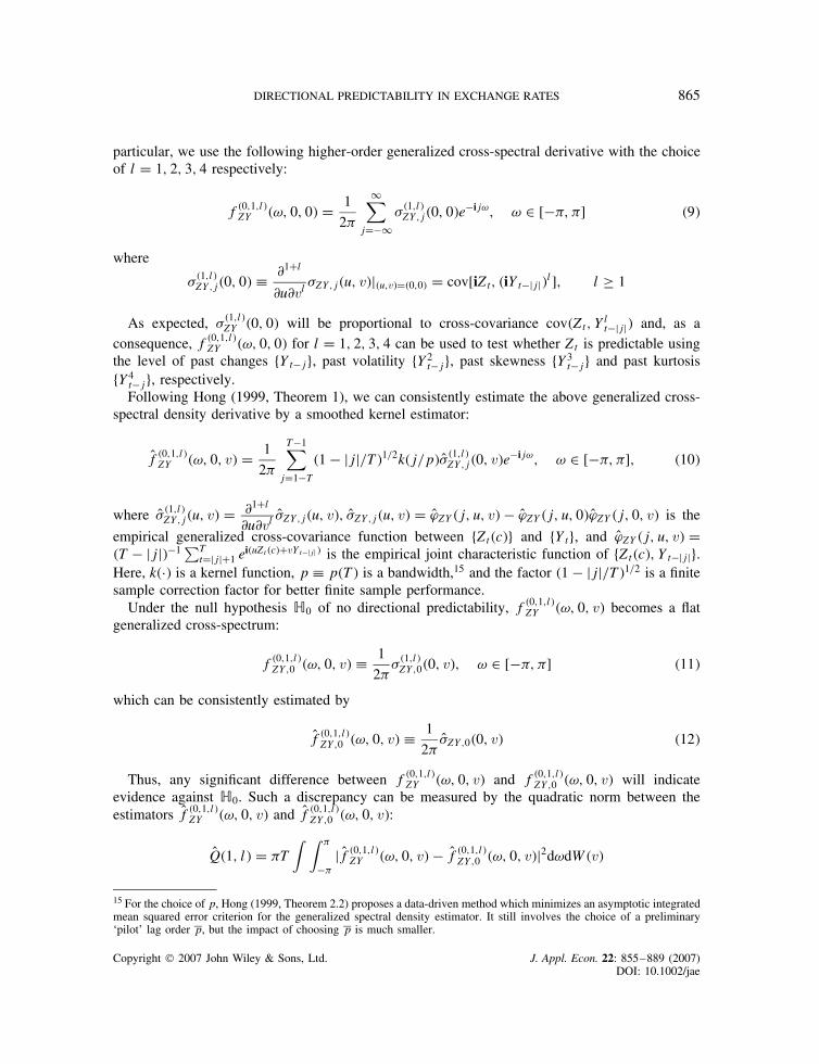
particular, we use the following higher-order generalized cross-spectral derivative with the choiceof l D 1, 2, 3, 4 respectively:

f�0,1,l�ZY �ω, 0, 0� D 1

2�

1∑jD�1

��1,l�ZY,j�0, 0�e�ijω, ω 2 [��, �] �9�

where

��1,l�ZY,j�0, 0� � ∂1Cl

∂u∂vl �ZY,j�u, v�j�u,v�D�0,0� D cov[iZt, �iYt�jjj�l], l ½ 1

As expected, ��1,l�ZY �0, 0� will be proportional to cross-covariance cov�Zt, Yl

t�jjj� and, as aconsequence, f�0,1,l�

ZY �ω, 0, 0� for l D 1, 2, 3, 4 can be used to test whether Zt is predictable usingthe level of past changes fYt�jg, past volatility fY2

t�jg, past skewness fY3t�jg and past kurtosis

fY4t�jg, respectively.Following Hong (1999, Theorem 1), we can consistently estimate the above generalized cross-

spectral density derivative by a smoothed kernel estimator:

Of�0,1,l�ZY �ω, 0, v� D 1

2�

T�1∑jD1�T

�1 � jjj/T�1/2k�j/p� O��1,l�ZY,j�0, v�e�ijω, ω 2 [��, �], �10�

where O��1,l�ZY,j�u, v� D ∂1Cl

∂u∂vl O�ZY,j�u, v�, O�ZY,j�u, v� D OϕZY�j, u, v� � OϕZY�j, u, 0� OϕZY�j, 0, v� is the

empirical generalized cross-covariance function between fZt�c�g and fYtg, and OϕZY�j, u, v� D�T � jjj��1 ∑T

tDjjjC1 ei�uZt�c�CvYt�jjj� is the empirical joint characteristic function of fZt�c�, Yt�jjjg.Here, k�Ð� is a kernel function, p � p�T� is a bandwidth,15 and the factor �1 � jjj/T�1/2 is a finitesample correction factor for better finite sample performance.

Under the null hypothesis �0 of no directional predictability, f�0,1,l�ZY �ω, 0, v� becomes a flat

generalized cross-spectrum:

f�0,1,l�ZY,0 �ω, 0, v� � 1

2��1,l�

ZY,0�0, v�, ω 2 [��, �] �11�

which can be consistently estimated by

Of�0,1,l�ZY,0 �ω, 0, v� � 1

2�O�ZY,0�0, v� �12�

Thus, any significant difference between f�0,1,l�ZY �ω, 0, v� and f�0,1,l�

ZY,0 �ω, 0, v� will indicateevidence against �0. Such a discrepancy can be measured by the quadratic norm between theestimators Of�0,1,l�

ZY �ω, 0, v� and Of�0,1,l�ZY,0 �ω, 0, v�:

OQ�1, l� D �T∫ ∫ �

��j Of�0,1,l�

ZY �ω, 0, v� � Of�0,1,l�ZY,0 �ω, 0, v�j2dωdW�v�

15 For the choice of p, Hong (1999, Theorem 2.2) proposes a data-driven method which minimizes an asymptotic integratedmean squared error criterion for the generalized spectral density estimator. It still involves the choice of a preliminary‘pilot’ lag order p, but the impact of choosing p is much smaller.



DT�1∑jD1

k2�j/p��T � j�∫

j O��1,l�ZY,j�0, v�j2dW�v� �13�

where W�Ð� is a positive and nondecreasing weighting function, and the unspecified integral istaken over the support of W�Ð�.16 Then, the resulting test statistic is a standardized version of thecumulative sum of OQ�1, l�:

MZY�1, l� D OQ�1, l� � OCZY�1, l�

T�1∑jD1

k2�j/p�

/[ ODZY�1, l�]1/2 �14�

where the centering and scaling factors OCZY�1, l� and ODZY�1, l� are approximately the mean andthe variance of the quadratic form T OQ in (13) and their expressions are given in Hong and Chung(2006). Under �0, the statistic OMZY�1, l� is asymptotically N(0, 1). It generally diverges to positiveinfinity under the alternatives to �0, and thus allows us to use upper-tailed N(0, 1) critical valuesas appropriate critical values (see Hong and Chung, 2006, for details).

The last stage of our stepwise testing procedure is to examine whether the directions of pastreturns fZt�j, j > 0g can be useful to predict the directions of future returns fZtg. This aims toexplore a growing empirical evidence of pattern anomalies in foreign exchange markets, such asover/underreaction (e.g., Larson and Madura, 2001, and references therein) and long swing (Engeland Hamilton, 1990). The former indicates short-term price reversal (or continuation) followinglarge price changes, while the latter presents periodic short-term foreign exchange rate movementsin one direction. In a period of time where these pattern anomalies are found, the successivedirections of foreign exchange rate movements can be examined as a function of past directions.

To capture serial dependence in the univariate time series fZt�c�g that consists of past and futuredirections, we use the generalized spectral density function of Hong (1999):

fZZ�ω, u, v� D 1

2�

1∑jD�1

�ZZ,j�u, v�e�ijω �15�

where the generalized covariance function is

�ZZ,j�u, v� D cov�eiuZt�c�, eivZt�jjj�c�� 16�

The associated test statistic MZZ�1, 0� to test �0 : E�ZtjZt�jjj� D E�Zt� a.s. can be derived ina similar manner to the test statistic MZY�1, 0�: we compare a consistent kernel estimator for the(1, 0)th order univariate generalized spectral derivative f�0,1,0�

ZZ �ω, 0, v� and a consistent estimatorfor the flat spectrum f�0,1,0�

ZZ,0 �ω, u, v�.17 Likewise, the MZZ�1, 0� test has the same N(0, 1) limitdistribution as MZY�1, l� (Hong, 1999).

16 As different choices of the derivative orders �m, l� yield tests of various hypotheses, different W�Ð� may be selecteddepending on which hypothesis is of interest. For the omnibus test MZY�1, 0�, we put W�Ð� D W0�Ð�, where W0�Ð� is theN(0, 1) CDF. For the separate tests MZY�1, l� with l ½ 1, we put W0�Ð� D υ�Ð�, where υ�Ð� is the Dirac delta function;namely, υ�u� D 0 for all u 6D 0 and

∫ 1�1 υ�u�du D 1. For further discussion, see Hong (1999).

17 Alternatively, one could test directional predictability by testing the i.i.d. property for fZt�c�g. Because the directionindicator Zt�c� is a Bernoulli random variable taking value 0 or 1, it is independent of It�1 if Zt�c� is not predictableusing It�1. Thus, if evidence against i.i.d. is found for fZt�c�g, one can conclude that the direction of returns is predictableusing the past history of the return directions fZt�1�c�, Zt�2�c�, . . .g. See Hong and Chung (2006) for further discussion.



Finally, it is straightforward to test whether interest rate differentials fIDtg are useful inpredicting the direction of foreign exchange rate returns fZtg. We will repeat the above evaluationmeasures, but with change of argument Yt D IDt. Accordingly, we denote MZID�1, 0� as anomnibus test for �0 of (4), and MZID�1, l� with l D 1, 2, 3, 4 and MZZID �1, 0� as separate tests tocheck whether fZtg is predictable using the level, volatility, skewness, kurtosis and directions ofpast interest rate differentials fIDt�jg, respectively.

3.2. Tests for the Direction of Joint Changes in Two Currencies

Our aim is now to gauge directional predictability of joint changes in two currencies. Intuitively,previous measures fZY�ω, u, v� and fZZ�ω, u, v� cannot be directly applicable when there aremore than two variables involved (as is the case when we explore the directional predictabilityof joint changes in two currencies using their return series fY1t, Y2tg).18 For this purpose, we willuse the multivariate generalized cross-spectral density below.

Suppose we have a strictly stationary time series process fZt, Y1t, Y2tg, and define the general-ized cross-covariance function between fZtg and fY1t�j, Y2t�j, j > 0g as

�ZY1Y2,j�u, v, � � cov�eiuZt , ei�vY1t�jjjCY2t�jjj��, j D 0, š1, . . . �17�

where u, v, 2 ��1, 1�, i D p�1. By the Fourier transform of �ZY1Y2,j�u, v, �, we readilyobtain the generalized cross-spectral density between fZtg and fY1t�j, Y2t�j, j > 0g:

fZY1Y2�ω, u, v, � � 1

2�

1∑jD�1

�ZY1Y2,j�u, v, �e�ijω, ω 2 [��, �] �18�

Like �ZY�u, v� and �ZZ�u, v�, because �ZY1Y2�u, v, � D 0 for all u, v, 2 ��1, 1� if and onlyif fZtg and fY1t�j, Y2t�jg are mutually independent, �ZY1Y2 �u, v, � can capture any type of pairwisecross-dependence between fZtg and fY1t�j, Y2t�jg, and so is fZY1Y2�ω, u, v, �. As a result, wecan use fZY1Y2�ω, u, v, � to explore how Zt depends on the entire past history of two currencyreturns fY1t�j, Y2t�j, j > 0g.

When EjZtj2m < 1 and E�jY1tj2l C jY2tj2l� < 1, we can introduce the generalized cross-spectral density derivative between fZtg and fY1t�j, Y2t�j, j > 0g by defining

f�0,m,l,l�ZY1Y2

�ω, u, v, � � ∂mC2l

∂um∂vl∂l fZY1Y2�ω, u, v, � D 1

2�

1∑jD�1

��m,l,l�ZY1Y2,j�u, v, �e�ijω, m, l ½ 0

�19�As before, our test statistics for the direction of joint changes will be based on comparison

via the quadratic form between two cross-spectral derivative estimators Of�0,1,l,l�ZY1Y2

�ω, u, v, � andOf�0,1,l,l�

ZY1Y2,0�ω, u, v, �, where the latter is implied by the null hypothesis �0 of no directionalpredictability:

OQ�1, l, l� D �T∫ ∫ ∫ �

��j Of�0,1,l,l�

ZY1Y2�ω, 0, v, � � Of�0,1,l,l�

ZY1Y2,0�ω, 0, v, �j2dωdW�v�dW��

18 For notational simplicity, we use the same notation Z for the direction indicator of joint changes in this section.



DT�1∑jD1

k2�j/p��T � j�∫ ∫

j O��1,l,l�ZY1Y2,j�0, v, �j2dW�v�dW�� 20�

Accordingly, we have the test statistic

MZY1Y2 �1, l, l� D OQ�1, l, l� � OCZY1Y2�1, l, l�

T�1∑jD1

k2�j/p�

/[ ODZY1Y2�1, l, l�]1/2 �21�

where

OCZY1Y2�1, l, l� D O��c�[1 � O��c�]∫

j O��l,l�Y1Y2,0�v, �v�j2dW�v�

ODZY1Y2�1, l, l� D 2 O�2�c�[1 � O��c�]2T�2∑jD1

T�2∑D1

k2�j/p�k2�/p�∫ ∫

j O��l,l�Y1Y2,j��u, v�j2dW�u�dW�v�

and O�Y1Y2,j�u, v� D OϕY1Y2,j�u, v� � OϕY1Y2,j�u, 0� OϕY1Y2,j�0, v� is the empirical generalized autoco-variance function of fY1t, Y2tg, O��c� D T�1 ∑T

tD1 Zt�c� is the sample proportion for fY1t > c, Y2t >cg. All the MZY1Y2�1, l, l� tests have the same N(0, 1) limit distribution as MZY�1, l�.19

Once again, we conduct the stepwise testing procedure in a manner analogous to the previouscase: we begin with a hypothesis test to check whether E�ZtjY1t�jjj, Y2t�jjj� D E�Zt�, j D0, š1, . . ., using the omnibus test statistic MZY1Y2�1, 0, 0�. We then proceed to use the derivativetests MZY1Y2�1, l, l�, for l D 1, 2, 3, 4 to search possible sources of directional predictability ofjoint changes. Finally, we will use the MZZY1 ZY2

�1, 0, 0� test to examine whether the directions ofpast returns can be used to predict the direction of future joint changes.

We further perform the analyses via fZY1 �ω, u, v� and fZY2�ω, u, v�, which will tell us whetherthe direction of joint changes in two currencies is predictable, using individual returns fY1t�jg andfY2t�jg, respectively. Also, the same test procedures will be repeated for examining the directionof joint changes based on interest rate differentials, using two interest rate differential seriesfID1t�j, ID2t�jg jointly and individually. With these versatile test sets, we can better characterizethe nature of directional predictability of joint changes in foreign exchange markets.

4. DATA

Daily foreign exchange spot rates in currency units per US dollar and daily foreign currencyfutures prices for the Australia dollar (AD), the Canadian dollar (CD), the British pound (BP), theJapanese yen (JY), the Swiss franc (SF) and the Deutschemark (DM) are employed to examinedirectional predictability of the foreign exchange market. Foreign exchange spot rates are noonbuying rates in New York for cable transfers payable and available from the Board of Governors ofthe Federal Reserve System (www.federalreserve.gov). Futures prices for the same six currencies,denoted by an F-prefix on each symbol, are daily closing prices traded at the Chicago Mercantile

19 The proof is a straightforward extension of that given in Hong and Chung (2006).



Exchange (CME) and obtained from Datastream. We compute returns as the percent logarithmicdifference

Yt D 100 ln�StC1/St�,

where St is an exchange spot rate or futures price.20

To construct interest rate differentials rt � rŁt , we use the 3-month London InterBank Offered

Rate (LIBOR) for the US dollar (USD) and all six currencies as the domestic risk-free interest ratert and the foreign risk-free interest rate rŁ

t , respectively. Daily observations on the interest ratescome, when available, from Datastream.21 Table I reports descriptive statistics of the sample. Thefirst two panels include some basic statistics for the returns on spot rates and futures prices, whichhave the same starting date, December 1 1987, but have different ending dates for DM. Uponthe introduction of the euro and the irrevocably fixed conversion rates, the DM data stop afterDecember 31 1998 and December 14 2001, respectively, for spot rates and future prices. Totalobservations in futures prices are slightly more than those in spot rates, due to different tradingdays in each market.

The sample means of returns are marginally different across currencies and markets (i.e., spotrates and futures prices), but they are all close to zero. CD is most stable for both spot and futures,with a standard deviation that is roughly half the size of other currencies. There is evidence ofleptokurticity, but there is no clear evidence of negative skewness (particularly for FJY).22

The statistics for interest rate differentials, reported in the last panel in Table I, are computedover the same period to match the ending date of the returns in both spot and futures markets.In general, interest rate differentials have a sizeable non-zero sample mean: the mean interest ratedifferentials of AD, CD and BP (vis-a-vis USD) are negative, which implies risk-free interest ratesfor AD, CD and BP are, on average, higher than that for USD. In contrast, the mean interest ratedifferentials of JY, SF and DM (vis-a-vis USD) are positive (particularly for JY). Compared to theexchange rate changes, interest rate differentials are much smoother and less volatile. It remains,however, to see whether the relatively tranquil nature of interest rate differentials can be used toforecast the direction of foreign exchange returns. For interest rate differentials, there is evidenceof negative skewness, but there is no clear evidence of excess kurtosis (except for AD).

5. EMPIRICAL EVIDENCE

5.1. Directional Predictability of Changes in a Single Currency

We now use the generalized cross-spectral (GCS) tests to examine directional predictability ofindividual currency returns and its possible sources. We first consider the following directionindicators:

ZCt �c� D 1�Yt > c�, and Z�

t �c� D 1�Yt < �c�

20 Note that our definition of returns may be nominal (rather than actual) values to study solely the direction of the changesin the underlying spot (or futures) price: relative rates of return on US dolloars comprise both (nominal) price changesand interest rate differentials.21 For the Canadian dolloar, we use the 3-month Treasury Bill rates.22 These stylized facts differ from those of the daily returns in stock markets. The returns in stock markets commonlyexhibit leptokurtosis, fat tails and negative skewness (see, for example, Fama, 1965). For more discussion on the stylizedfacts and statistical properties of the daily returns from foreign exchange markets, we refer to Hsieh (1988) and de Vries(1994).



Table I. Summary statistics for sample data

Symbols Ending date Obs. Mean (%) SD (%) Skew. Kurt. r1�1� r2�1�

SpotAD 2003/04/30 3875 �0.003 0.612 �0.285 8.487 0.012 0.209CD 2003/04/30 3875 0.002 0.310 0.018 5.278 0.036 0.128BP 2003/04/30 3875 �0.003 0.591 �0.265 5.597 0.060 0.142JY 2003/04/30 3875 �0.003 0.708 �0.477 7.084 0.035 0.209SF 2003/04/30 3875 0.000 0.721 �0.119 4.499 0.027 0.123DM 1998/12/31 2787 0.001 0.668 0.038 4.778 0.037 0.152

FuturesFAD 2003/04/30 3901 �0.003 0.640 �0.256 6.614 �0.010 0.060FCD 2003/04/30 3901 �0.002 0.325 �0.145 5.391 0.002 0.145FBP 2003/04/30 3901 �0.003 0.635 �0.220 6.548 0.000 0.078FJY 2003/04/30 3901 0.003 0.758 0.664 10.451 �0.010 0.100FSF 2003/04/30 3901 0.000 0.752 0.091 4.811 �0.005 0.097FDM 2001/12/14 3557 �0.008 0.703 �0.057 5.256 �0.005 0.061

Interest rate differentialsr � rŁ�AD� 2003/04/30 3901 �0.023 0.025 �0.925 3.359 0.999 0.999r � rŁ�CD� 2003/04/30 3901 �0.008 0.019 �0.188 2.472 0.999 0.997r � rŁ�BP� 2003/04/30 3901 �0.024 0.022 �0.774 2.407 0.999 0.998r � rŁ�JY� 2003/04/30 3901 0.030 0.024 �0.423 1.866 1.000 0.999r � rŁ�SF� 2003/04/30 3901 0.015 0.027 �0.627 2.391 1.000 0.998r � rŁ�DM� 1998/12/31 2787 0.003 0.030 �0.655 2.113 0.999 0.999

2001/12/14 3557 0.000 0.028 �0.883 2.603 0.999 0.999

Notes:

1. Starting date for all spots and futures is December 1 1987.2. Obs., sample size (T); SD, standard deviation; Skew., skewness; Kurt., kurtosis.3. r1�1� and r2�1� are the first-order sample autocorrelation in returns and squared returns, respectively.4. r and rŁ denote the domestic (US) and foreign risk-free interest rates, respectively.

for c D 0, 0.5, 1, in units of the sample standard deviation of fYtg.23 Here, two types of indicatorfunction are designed to examine dynamic characteristics of directional movement in up anddown markets,24 while three threshold values are used to capture different magnitudes of changesin returns. In this paper, we mainly focus on pairwise cross-dependencies between Zt�c� and twokey variables: past returns fYt�jg and past interest rate differentials fIDt�j D rt�j � rŁ

t�jg, wherert is the domestic (US) risk-free interest rate and rŁ

t is the foreign risk-free interest rate at time t.We further rescale interest rate differentials centered at 0 to synchronize the levels of interest ratedifferentials across different countries.

We first examine directional predictability using the past history of fYtg. Table II reports thetest statistics MZY�1, l� for l D 0, 1, 2, 3, 4 and MZZ�1, 0� with the preliminary lag order p D 21

23 In this study, we do not consider c higher than one; the sample frequency that price changes are higher than one samplestandard deviation of fYtg is relatively low, and so this may reduce the statistical power of the test. The price limits in thefutures market make the use of higher threshold values even more undesirable. Brennan (1986) and Kodres (1993), usinga sign test, point out that price limits are more likely clustered in the same direction. Therefore, it may lead to spuriousfindings when we consider the stochastic behavior of directional movements of significantly higher changes.24 McQueen et al. (1996) find evidence of different autocorrelations in returns between up and down stock markets.



and the Bartlett kernel.25 Note, for comparison, that GCS tests are asymptotically one-sided N(0,1) tests and thus upper-tailed N(0, 1) critical values should be used, which are 1.65 and 2.33 atthe 5% and 1% significance levels, respectively.

The first top panel reports the omnibus MZY�1, 0� statistic, checking whether the directions ofeach currency return is predictable using its own past returns fYt�j, j > 0g. For all individualcurrency returns in both spot and futures markets, there exists strong evidence of directionalpredictability. Except for FSF and FDM, the MZY�1, 0� statistic value becomes larger as thresholdc increases, suggesting that the directions of large returns are easier to predict than the directionsof small returns using past returns. Comparing the spot and futures markets, we find that thedirections of the returns in the futures market are generally easier to predict with zero threshold�c D 0�. In contrast, when c D 1, the evidence is stronger for those in the spot market in mostcases. Further, there is no clear evidence that the direction of negative returns is easier to predictthan that of positive returns, using past returns. Among other things, the directions of AD, CD andBP in both spot and futures markets (respectively, FAD, FCD and FBP) are considerably easierto predict, especially with large thresholds (c D 0.5, 1).

The remaining panels in Table II examine possible sources of the documented directionalpredictability. We report the test statistics MZY�1, l� for l D 1, 2, 3, 4 and MZZ�1, 0�. These teststatistics can tell us to what extent past returns contain useful information for predicting thedirection of future returns. Specifically, each test statistic shows whether the direction of negativeand positive returns (left to right) can be predicted using the level, volatility, skewness, kurtosisand the direction of past returns (top to bottom), respectively. As shown in MZY�1, 1�, the level ofpast returns Yt�jjj has not been shown to be very useful in predicting the directions of individualcurrency returns, because no clear pattern of statistical significance emerges for the MZY�1, 1� test.In contrast, MZY�1, 2� shows strong evidence that past volatility is a valuable source of informationabout directional predictability of individual currency returns, particularly with large thresholds�c D 0.5, 1�. Like MZY�1, 0�, the test statistic MZY�1, 2� is monotonically increasing in thresholdlevel c, except for the direction of positive changes in FSF. Moreover, using past volatility, it isgenerally easier to predict the direction of negative returns than that of positive returns, and thedirections of the returns in the spot market than those in the futures market.

Next, MZY�1, 3� and MZY�1, 4� display patterns similar to MZY�1, 2�, and these similarities aremuch clearer for the statistic MZY�1, 4�. There is generally consistent evidence that the directionof large returns �c D 0.5, 1� is predictable using past skewness and kurtosis. Greater directionalpredictability is found in the spot market than in the futures market. However, unlike MZY�1, 2�,there seems no clear evidence that the direction of negative returns is easier to predict than thatof positive returns using past skewness and kurtosis of individual currency returns.

Finally, like MZY�1, 0�, the MZZ�1, 0� test indicates that the directions of future individualcurrency returns are predictable using the directions of past individual currency returns, and becomemore predictable with larger thresholds. It is also easier to predict the directions of the returnsin spot rates than in futures prices with large thresholds (c D 0.5, 1). The MZZ�1, 0� test furthersuggests that the direction of negative returns is easier to predict than that of positive returns,using the directions of past returns.

In light of the above results, nonlinear models can be more useful in predicting the foreignexchange dynamics than linear regression models. For example, the significance of the MZZ�1, 0�

25 For robust results, we also use preliminary lag orders p from 11 to 51. The results are very similar, and for reasons ofspace we only report the results with p D 21.



Table II. GCS test statistics for changes in single currency spot and futures (p D 21): using past returns

Positive direction Negative direction

Currency c D 0 c D 0.5 c D 1.0 c D 0 c D 0.5 c D 1.0

MZY�1, 0�AD 4.93 10.84 15.48 4.96 9.73 16.52CD 1.80 10.45 10.78 1.22 8.23 17.56BP �0.38 6.37 13.97 �0.10 17.47 22.68JY 0.26 3.05 7.23 0.60 7.39 12.18SF 1.72 4.10 6.43 1.82 1.90 4.23DM �0.16 8.46 13.58 �0.04 1.64 8.41

FAD 6.20 11.22 10.70 5.74 9.66 12.76FCD 0.39 10.13 13.67 0.01 8.03 8.09FBP 2.61 6.19 9.95 3.72 15.54 19.38FJY 0.90 6.20 9.13 0.17 7.97 11.13FSF 5.11 0.13 3.69 5.51 3.69 4.08FDM 4.03 0.18 1.29 4.79 4.44 3.39

MZY�1, 1�AD 3.69 3.15 2.12 4.21 2.04 3.75CD 2.07 1.31 2.14 1.86 2.20 0.74BP �0.13 1.88 5.48 0.10 3.00 8.12JY 0.42 �0.02 1.11 0.50 2.15 7.20SF 0.92 1.43 0.03 1.20 1.23 3.15DM �0.56 2.45 0.03 �0.09 0.58 0.82

FAD 7.89 5.04 3.80 5.40 1.60 0.08FCD 0.42 1.15 0.71 �0.81 0.35 0.55FBP 2.23 2.31 1.07 1.59 0.46 3.08FJY 1.71 0.96 4.58 1.22 2.63 5.38FSF 6.24 �0.71 3.54 6.47 5.17 0.64FDM 2.76 �0.70 �0.40 3.62 1.68 �0.63

MZY�1, 2�AD 0.34 6.36 14.68 0.31 7.98 15.28CD �0.06 9.30 16.32 �0.54 9.78 30.76BP 0.69 10.26 25.90 0.92 27.60 46.19JY �1.34 8.40 21.71 �1.34 7.87 26.11SF 1.21 3.84 16.60 1.26 8.52 12.94DM 0.58 8.62 28.84 �0.10 7.31 22.00

FAD �1.09 4.60 12.14 �0.66 7.21 13.43FCD �0.98 15.81 21.59 �0.54 7.46 9.17FBP 1.24 7.18 15.54 1.93 20.51 36.94FJY �0.54 6.25 15.81 �0.39 7.79 18.34FSF 0.12 3.00 1.47 0.15 2.42 12.24FDM �0.28 1.97 2.06 �0.04 1.96 6.57

MZY�1, 3�AD �0.21 1.33 3.41 �0.29 �0.72 0.92CD 0.13 �0.92 0.29 0.08 0.45 1.88BP 2.79 2.08 7.40 2.68 7.04 18.03JY �0.41 0.43 4.01 �0.37 1.61 9.42SF 1.39 3.45 6.78 1.36 0.99 4.18DM 1.03 3.48 3.95 1.50 0.79 2.16

FAD 1.32 0.25 �1.01 1.14 2.39 2.45FCD �1.42 �0.77 �0.01 �1.50 �1.31 �0.09FBP �0.33 �0.28 1.82 �0.36 0.91 2.11FJY �0.62 0.38 5.83 �0.57 �0.03 3.04FSF 2.61 0.13 0.85 2.64 2.70 1.45FDM 0.15 �0.28 �0.21 0.32 0.09 1.24



Table II. (Continued )



MZY�1, 4�AD 1.47 2.74 7.04 1.35 4.84 7.43CD �1.19 1.71 5.32 �1.28 1.52 8.86BP 0.68 2.39 8.37 0.96 12.21 24.22JY �0.13 1.03 7.40 �0.07 3.77 16.74SF 0.53 0.46 8.82 0.59 5.71 9.13DM 0.51 2.80 14.76 �0.02 4.44 13.58

FAD �0.53 0.32 5.73 �0.45 1.31 5.03FCD �1.32 6.64 9.37 �1.08 1.94 2.97FBP 0.27 1.69 3.35 0.62 6.58 12.90FJY �0.24 2.46 8.69 �0.35 0.43 3.41FSF 0.26 0.57 �0.56 0.53 1.05 7.25FDM �0.28 �0.15 �0.41 �0.31 1.29 2.16

MZZ�1, 0�AD 1.65 2.50 0.42 1.98 4.69 13.40CD 1.92 10.09 9.49 1.52 0.39 9.84BP �1.10 0.21 6.11 �1.03 8.08 22.66JY �0.63 2.51 5.54 �0.47 7.06 13.32SF 1.82 �1.07 5.60 1.88 1.33 2.38DM �1.16 0.04 7.89 �0.73 0.62 6.74

FAD 5.56 2.21 1.44 3.80 2.02 10.53FCD �0.46 1.03 5.16 �1.03 4.67 3.20FBP 0.29 0.88 2.04 0.03 7.56 18.28FJY 0.50 5.45 8.58 0.24 2.68 3.84FSF 2.61 �0.24 3.71 3.65 2.98 2.59FDM 1.76 �0.03 2.06 2.95 2.02 2.57

Notes:

1. GCS tests are asymptotically one-sided N(0,1) tests and thus upper-tailed asymptotic critical values may also be used,which are 1.65 and 2.33 at the 5% and 1% levels, respectively. M(1,l) represents test statistics on the martingale test,serial correlation test, ARCH-in-mean test, skewness-in-mean test and kurtosis-in-mean test for l D 0, . . . 4, respectively.

2. Currency returns are defined by 100 ln�St/St�1� where St is an exchange spot rate or futures price.3. A preliminary bandwidth, p is crucial to run GCS tests. We have computed GCS test statistics for p D 11, . . . , 50, but

reported only for the value of p D 21 to save space.4. A threshold value c is introduced to forecast bigger changes. A higher threshold value of c implies a bigger change in

rate or price.

test suggests that the past own directions are useful in predicting future directions of exchangerate changes. This might be due to directional clustering, implying that an autologistic modelof direction indicators may have some predictive ability for future directions. Nevertheless,the significance of separate inference tests MZY�1, l� does not necessarily imply that a simplepolynomial model in fYt�jg will forecast the direction of exchange rate changes well, particularlyin an out-of-sample context (see Hong and Lee, 2006, for an out-of-sample forecasting exercisefor foreign exchange rates). A high-order polynomial model may not be robust to outliers in atime series context, and foreign exchange returns may have a more subtle nonlinear dynamics,although the powers of lagged variable Yt�j have predictable ability. For example, a significant



directional dependence on Y2t�j may be due to a bilinear or nonlinear moving average-type

structure. Obviously, a comprehensive investigation of modeling and forecasting the nonlineardynamics in foreign exchange rates is needed, but this is beyond the scope of the presentpaper.

We now turn to examining whether directional predictability of individual currency returnscan be explained by interest rate differentials. Table III reports the test statistics MZID�1, l�for l D 0, 1, 2, 3, 4 and MZZID �1, 0�. The omnibus test MZID�1, 0� checks whether interest ratedifferentials can be used to forecast the directions of individual currency returns, and variousderivative tests MZID�1, l� for l D 1, 2, 3, 4 examine specific types of cross-dependence betweenZt and f�IDt�j�l, j > 0g. Finally, the MZZID �1, 0� statistic checks whether E�ZtjZID,t�j� D E�Zt�for all j > 0; namely it checks whether the direction of past interest rate differentials can be usedto predict the direction of future returns in foreign exchange markets. As indicated in MZID�1, 0�,there exists strong evidence of directional predictability using interest rate differentials, except forthe positive direction of FJY and the negative direction of JY. The MZID�1, 0� test also suggeststhat the directions of the returns with large thresholds �c D 0.5, 1� are much easier to predict thanthose with zero threshold using interest rate differentials, although the value of MZID�1, 0� is notmonotonically increasing in threshold c. These results provide considerable empirical support forthe idea that interest rate differentials are a useful predictor for the directions of future foreignexchange rate changes.

Next, MZID�1, 1� shows strong evidence that the direction of individual currency returns ispredictable using the level of interest rate differentials. Interestingly, in many cases the descriptivepattern of the statistical significance in the MZID�1, 1� test closely resembles that in the MZID�1, 0�test. For example, the values of MZID�1, 0� and MZID�1, 1� for AD and FAD exhibit a \-shapefunction of c for the negative directions. On the other hand, those of FCD exhibit a [-shape functionof c for positive directions, and are monotonically decreasing in threshold c for negative directions.Since this pattern similarity associated with MZID�1, 0� is not found for the remaining GCS tests, itappears that a deriving source for directional predictability using interest rate differentials may bethe time-varying conditional mean of interest rate differentials. This is consistent with Lothian andWu’s (2003) finding that the level of interest rate differentials plays an important role in explainingpredictability of exchange rate movements. They point out that large interest rate differentials havemuch stronger forecasting power of foreign exchange rates than small interest rate differentials(see also Flood and Rose, 2002; Huisman et al., 1998).

Likewise, MZID�1, 2� indicates that, except for JY and FJY, the direction of individual currencyreturns is predictable using past volatility of interest rate differentials. However, the evidenceis not strong and the overall statistical significance is much weaker than that for the MZY�1, 2�test—we have seen that the past volatility of the returns is most helpful in predicting the directionof future returns. Taken together, these findings suggest that the smooth and symmetric nature ofthe volatility of interest rate differentials may result in weaker impact on directional predictabilitythan the volatility of individual currency returns.

Finally, MZID�1, 3� and MZID�1, 4� show limited evidence of directional predictability fromskewness and kurtosis of past interest rate differentials. In fact, there are many cases whereneither skewness nor kurtosis of past interest rate differentials is useful in predicting the directionof individual currency returns (e.g., AD in both spot and futures markets). On the other hand,MZZID �1, 0� shows strong evidence that the direction of past interest rate differentials can beused to predict the direction of future individual currency returns. When compared to MZZ�1, 0�,



Table III. GCS test statistics for changes in single currency spot and futures (p D 21): using interest ratedifferentials



MZID�1, 0�AD 6.41 3.71 7.14 7.01 21.49 15.65CD 7.00 7.93 4.23 7.02 0.74 6.76BP 1.29 24.69 32.28 1.13 6.64 26.84JY 1.36 3.78 15.39 0.08 �0.75 0.23SF 4.24 2.69 4.34 3.70 9.09 13.30DM 0.65 3.58 10.51 0.51 6.28 11.84

FAD 3.21 2.49 2.68 9.04 15.25 14.90FCD 10.34 1.79 8.29 19.04 7.80 5.73FBP 0.02 24.01 34.17 2.53 13.11 25.33FJY 1.92 �0.58 0.83 1.99 11.92 14.31FSF 3.07 9.63 7.83 5.79 1.51 4.37FDM 3.61 10.93 5.01 2.02 1.88 3.18

MZID�1, 1�AD 3.04 �0.06 0.33 3.01 9.98 2.37CD 7.05 4.73 1.71 7.08 0.00 �0.56BP 1.55 25.46 26.40 1.18 2.93 23.73JY 1.58 3.73 13.76 0.14 �0.64 �0.21SF 4.38 �0.03 3.45 4.12 13.38 19.62DM 0.54 2.11 9.16 0.74 7.25 13.51

FAD 2.69 1.49 �0.70 5.98 6.29 2.48FCD 10.77 1.35 1.97 19.52 8.22 4.25FBP 0.77 23.63 29.76 3.91 8.58 20.55FJY 1.48 �0.63 �0.53 1.08 11.38 12.39FSF 2.01 13.63 12.90 4.59 �0.37 3.87FDM 4.55 12.93 6.96 2.72 0.88 2.16

MZID�1, 2�AD �0.21 2.35 3.11 0.33 2.11 5.92CD 0.36 2.11 2.35 0.48 �0.24 5.29BP 3.24 12.16 7.41 3.17 �0.47 8.44JY �0.34 �0.71 0.80 �0.66 �0.21 �0.35SF �0.32 3.62 7.41 �0.06 4.20 7.00DM �0.67 1.83 8.35 �0.69 �0.21 5.31

FAD �0.70 3.34 2.45 �0.69 2.08 5.43FCD 1.12 0.01 6.85 5.23 2.31 1.18FBP 0.20 10.05 10.63 3.33 0.30 5.76FJY �0.70 �0.29 �0.60 �0.60 �0.34 0.37FSF �0.70 3.91 6.37 �0.68 2.59 6.67FDM 0.28 2.07 2.35 0.04 2.38 3.10

MZID�1, 3�AD �0.70 �0.27 �0.32 �0.69 �0.31 �0.69CD 3.48 0.83 �0.15 3.59 1.53 0.26BP 3.63 18.74 10.38 3.29 �0.58 12.58JY 0.54 1.57 5.82 �0.46 �0.71 �0.61SF 2.92 0.60 5.75 3.28 13.10 17.05DM 0.63 0.59 6.96 0.94 4.87 10.83

FAD �0.13 1.58 �0.01 0.02 �0.45 �0.69FCD 6.35 1.96 �0.28 11.89 5.57 1.51FBP 1.43 15.20 14.43 6.12 0.94 8.22FJY �0.15 �0.69 �0.36 �0.51 5.24 4.43FSF 1.27 12.92 15.19 2.17 0.45 4.55FDM 2.70 8.26 5.82 1.69 0.67 1.51



Table III. (Continued )



MZID�1, 4�AD �0.26 �0.26 0.68 0.17 �0.39 0.38CD 1.13 1.52 0.94 1.37 �0.48 0.66BP 4.10 13.72 5.95 3.84 �0.52 8.37JY 0.19 �0.37 1.69 �0.51 �0.11 0.46SF 1.87 0.07 2.82 2.51 9.11 9.00DM �0.16 0.27 6.38 0.23 1.52 5.85

FAD �0.64 1.41 0.36 �0.68 �0.43 0.41FCD 2.83 �0.68 2.12 5.74 1.22 �0.29FBP 1.07 11.26 9.60 4.82 �0.04 4.64FJY �0.53 �0.16 �0.65 �0.71 0.92 1.16FSF 0.58 9.04 11.24 0.97 0.09 2.30FDM 1.26 4.52 3.66 0.89 0.85 1.49

MZZID �1, 0�AD 4.53 0.94 6.63 4.59 4.80 1.01CD 8.96 3.12 �0.43 9.13 0.38 4.81BP 0.33 15.52 1.03 �0.05 5.56 18.09JY 0.57 9.77 �0.24 �0.45 �0.71 �0.33SF 4.70 �0.54 �0.67 4.31 5.27 11.57DM �0.17 �0.26 �0.58 �0.07 2.51 15.42

FAD 1.80 �0.68 1.89 5.78 3.22 1.06FCD 13.85 2.77 0.48 20.11 10.58 8.13FBP 0.42 16.38 1.99 0.96 11.50 16.06FJY 2.53 �0.67 2.21 2.40 6.36 4.27FSF 2.89 13.62 1.88 5.76 1.60 15.25FDM 4.61 20.00 0.97 3.47 2.86 4.23

Notes:

1. GCS tests are asymptotically one-sided N(0,1) tests and thus upper-tailed asymptotic critical values may also be used,which are 1.65 and 2.33 at the 5% and 1% levels, respectively. M�1, l� represents test statistics on the martingale test,serial correlation test, ARCH-in-mean test, skewness-in-mean test and kurtosis-in-mean test for l D 0, . . . 4, respectively.

2. Interest rate differentials are defined by rt � rŁt where rt is the domestic (US) risk-free interest rate and rŁ

t is the foreignrisk-free interest rate.

3. A preliminary bandwidth p is crucial to run GCS tests. We have computed GCS test statistics for p D 11, . . . , 50, butreported only for the value of p D 21 to save space.

4. A threshold value c is introduced to forecast bigger changes. A higher threshold value of c implies a bigger change inrate or price.

the directions of past interest rate differentials are more useful to predict the directions of thereturns with zero threshold. Such differences are, however, attenuated with large thresholds�c D 0.5, 1�.

In summary, the GCS tests MZY�1, 0� and MZID�1, 0� show that the directions of the indi-vidual returns in spot and futures foreign exchange markets with any threshold are predictableusing past history of both returns and interest rate differentials. Moreover, this evidence isgenerally stronger for greater movements �c D 0.5, 1�. Our generalized cross-spectral deriva-tive tests show that the level, volatility, skewness, kurtosis and direction of past returns and



interest rate differentials are more or less useful in predicting the direction of individual cur-rency returns. In particular, based on past returns, although the generally insignificant statisticMZY�1, 1� indicates a weak predictive power of conditional mean dynamics for the directionof future returns, we can see from MZY�1, l� for l D 2, 3, 4 and MZZ�1, 0� that strong depen-dencies derived from higher order conditional moments and the directions of past returns canattribute to the documented directional predictability. Furthermore, our GCS test results basedon interest rate differentials suggest that the conditional mean dynamics of interest rate differ-entials contribute significantly to directional predictability, which provides an important policyimplication—the monetary authorities can have substantial influence on the foreign exchangemarkets as they can affect the direction of future foreign exchange rates through the domestic(foreign) currency and/or the domestic interest rate. This monetary policy may be more effec-tive with changes in the volatility of foreign exchange returns and/or the level of interest ratedifferentials.

5.2. Directional Predictability of Joint Changes in Two Currencies

We now examine directional predictability of returns co-movements in foreign exchange ratemarkets. Specifically, we are interested in the direction of joint changes in two currencies withineach spot market and each futures market.26 Consider individual returns fYktg, k D 1, 2, wherethe subscript k denotes currency k. A new direction indicator of joint changes is then defined asfollow:

ZCt �c� D 1�Y1t > c1, Y2t > c2�, c D �c1, c2�

Z�t �c� D 1�Y1t < �c1, Y2t < �c2�, c D �c1, c2�

for ck D 0, 0.5, 1, in units of the sample standard deviation of fYktg, k D 1, 2. As in the previoussection, ZC

t �c� and Z�t �c� can detect upward and downward market comovements, respectively.

Further, with nonzero thresholds (i.e., ck D 0.5, 1), these indicators are able to detect greaterco-movements between two currency returns.

In applying the GCS tests to directional predictability of joint changes, we use twofoldtests: (i) a test of directional predictability using the past returns of two currencies, checkingwhether E�ZtjY1t�j, Y2t�j� D E�Zt� for all j > 0; (ii) a test of directional predictability usingpast individual returns of each currency, checking whether E�ZtjYkt�j� D E�Zt� for all j > 0, andfor k D 1, 2. Naturally, the latter consists of two sets of GCS tests on the direction of changesin a single currency. Similar to Section 5.1, each of these GCS tests will be conducted with pastcurrency returns and interest rate differentials.

We first report the GCS test results based on past returns in Table IV. For reasons of space, weonly present the GCS test statistics for the direction of joint negative changes in the spot market.Overall, the patterns for the direction of joint positive changes are rather similar to those of jointnegative changes, though less significant at times. Likewise, the results for the futures market arelargely similar to those for the spot market, unless otherwise noted.27

Table IV consists of three sections: the first section provides the GCS test statistics usingpast returns of two currencies jointly (hereafter denoted as ‘joint returns’), while the remaining

26 One may be also interested in the joint changes between spot and futures markets.27 All (unreported) results are available upon request from the authors.



Table IV. GCS test statistics for negative joint changes in two currency spot rates (p D 21): using past returns

Joint returns Returns of Cc 1 of Cc 2

Cc1 Cc2 c D 0 c D 0.5 c D 1 c D 0 c D 0.5 c D 1 c D 0 c D 0.5 c D 1

AD CD MZY1Y2 �1, 0, 0� 0.87 1.96 4.69 MZYk �1, 0� 2.67 4.86 6.69 1.60 10.83 7.37MZY1Y2 �1, 1, 1� 0.76 �0.55 2.70 MZYk �1, 1� 1.22 1.72 �0.20 2.61 2.50 �0.37MZY1Y2 �1, 2, 2� �0.17 1.35 11.76 MZYk �1, 2� 0.07 �0.41 2.06 �0.03 12.15 16.84MZY1Y2 �1, 3, 3� �0.76 1.92 12.38 MZYk �1, 3� �0.86 �0.56 �0.05 0.16 2.46 1.60MZY1Y2 �1, 4, 4� �0.88 1.94 12.14 MZYk �1, 4� 0.95 �0.80 �0.50 �0.37 5.09 6.09MZZ1Z2 �1, 0, 0� 0.32 �0.86 8.80 MZZk �1, 0� 1.23 2.92 3.40 1.44 3.94 3.51

AD BP MZY1Y2 �1, 0, 0� 1.00 8.36 4.14 MZYk �1, 0� 3.44 4.39 3.90 �1.35 2.97 2.85MZY1Y2 �1, 1, 1� �0.64 4.73 9.25 MZYk �1, 1� 2.95 0.63 0.18 �0.88 �0.21 0.95MZY1Y2 �1, 2, 2� �1.17 3.32 12.17 MZYk �1, 2� 0.02 0.13 4.05 �0.81 2.68 4.50MZY1Y2 �1, 3, 3� �0.60 0.03 8.46 MZYk �1, 3� 0.07 �0.32 �0.36 0.16 0.88 0.88MZY1Y2 �1, 4, 4� �0.78 �0.35 7.11 MZYk �1, 4� 0.30 �0.53 0.91 �1.12 �0.45 0.87MZZ1Z2 �1, 0, 0� 0.49 2.78 3.37 MZZk �1, 0� 1.84 1.53 �0.72 �1.16 0.34 �0.64

AD JY MZY1Y2 �1, 0, 0� 2.25 7.64 11.38 MZYk �1, 0� 0.84 6.36 7.59 1.00 3.59 7.22MZY1Y2 �1, 1, 1� 4.40 5.54 8.99 MZYk �1, 1� 0.85 0.69 1.74 2.95 2.93 �1.20MZY1Y2 �1, 2, 2� 0.26 �1.32 �0.98 MZYk �1, 2� �0.43 3.09 4.30 �0.85 3.87 13.07MZY1Y2 �1, 3, 3� 0.56 �1.37 �1.40 MZYk �1, 3� 0.51 1.04 �0.90 0.02 0.53 0.18MZY1Y2 �1, 4, 4� 0.66 �1.35 �1.44 MZYk �1, 4� �0.18 0.17 �1.70 �0.13 �0.77 2.19MZZ1Z2 �1, 0, 0� 1.15 11.28 7.12 MZZk �1, 0� 0.76 1.69 1.40 0.14 �0.21 1.74

AD SF MZY1Y2 �1, 0, 0� 2.36 5.84 6.68 MZYk �1, 0� 0.98 6.01 8.60 2.03 0.45 1.05MZY1Y2 �1, 1, 1� 7.26 15.38 12.05 MZYk �1, 1� �0.68 0.84 4.91 2.25 0.04 0.54MZY1Y2 �1, 2, 2� 1.95 �0.40 1.83 MZYk �1, 2� �0.40 1.57 3.16 1.82 0.83 0.36MZY1Y2 �1, 3, 3� 0.92 �1.34 �1.26 MZYk �1, 3� 0.18 2.18 0.34 �0.21 0.39 0.04MZY1Y2 �1, 4, 4� 0.56 �1.38 �1.43 MZYk �1, 4� 0.37 0.84 �1.03 1.22 �0.56 �0.49MZZ1Z2 �1, 0, 0� 0.83 11.00 11.17 MZZk �1, 0� 0.01 3.47 1.17 2.29 �0.49 0.89

AD DM MZY1Y2 �1, 0, 0� 0.42 3.08 7.69 MZYk �1, 0� 0.42 2.06 6.80 �0.40 0.03 4.24MZY1Y2 �1, 1, 1� 3.09 12.12 18.86 MZYk �1, 1� �0.51 0.70 4.55 0.60 �0.42 2.18MZY1Y2 �1, 2, 2� 2.42 2.09 8.02 MZYk �1, 2� 0.66 2.96 2.36 0.69 4.05 3.07MZY1Y2 �1, 3, 3� 2.33 0.62 6.15 MZYk �1, 3� 0.93 3.61 0.48 0.41 3.89 1.53MZY1Y2 �1, 4, 4� 2.21 �0.48 3.13 MZYk �1, 4� �0.15 0.90 �0.73 0.63 4.64 0.88MZZ1Z2 �1, 0, 0� �1.04 5.75 9.36 MZZk �1, 0� �0.88 0.87 �0.57 0.60 �1.42 0.18

CD BP MZY1Y2 �1, 0, 0� 0.16 2.67 2.53 MZYk �1, 0� 2.18 3.06 3.87 �1.04 0.97 �0.08MZY1Y2 �1, 1, 1� 2.18 1.00 2.58 MZYk �1, 1� 1.31 3.40 1.55 0.61 0.93 2.47MZY1Y2 �1, 2, 2� �0.54 2.47 1.28 MZYk �1, 2� �1.24 1.40 4.04 �1.04 3.14 0.52MZY1Y2 �1, 3, 3� 0.75 0.80 1.02 MZYk �1, 3� �1.34 1.26 1.05 2.75 0.84 4.30MZY1Y2 �1, 4, 4� �1.16 0.42 �0.22 MZYk �1, 4� �0.48 1.32 1.88 �1.30 0.26 0.15MZZ1Z2 �1, 0, 0� 0.01 �0.97 1.67 MZZk �1, 0� 1.86 �0.73 1.78 �0.89 �0.26 1.67

CD JY MZY1Y2 �1, 0, 0� 0.76 3.40 6.73 MZYk �1, 0� 0.45 5.18 4.22 0.45 �0.08 5.42MZY1Y2 �1, 1, 1� 0.56 1.94 3.90 MZYk �1, 1� 1.58 2.53 1.23 0.77 �0.38 1.64MZY1Y2 �1, 2, 2� 0.15 0.83 4.47 MZYk �1, 2� �0.63 4.28 9.20 �0.60 0.13 6.97MZY1Y2 �1, 3, 3� �0.55 0.70 �0.17 MZYk �1, 3� 1.22 0.41 3.93 0.09 0.53 1.99MZY1Y2 �1, 4, 4� �0.27 0.29 0.09 MZYk �1, 4� �1.08 0.18 6.34 0.02 0.16 1.20MZZ1Z2 �1, 0, 0� �0.37 4.31 8.07 MZZk �1, 0� 0.40 2.45 2.03 �0.22 1.46 5.50

CD SF MZY1Y2 �1, 0, 0� 1.49 4.81 7.06 MZYk �1, 0� �0.41 3.41 6.11 2.67 2.17 3.81MZY1Y2 �1, 1, 1� 3.61 2.78 2.74 MZYk �1, 1� 1.26 0.99 1.59 3.10 0.40 2.24MZY1Y2 �1, 2, 2� �0.42 �0.58 �0.45 MZYk �1, 2� �1.23 3.19 6.73 �0.32 4.14 5.85MZY1Y2 �1, 3, 3� 0.01 �0.97 �1.38 MZYk �1, 3� 0.00 0.01 0.59 0.96 �0.21 0.13MZY1Y2 �1, 4, 4� �0.65 �1.34 �1.44 MZYk �1, 4� �0.95 1.04 1.31 �1.01 �0.06 1.82MZZ1Z2 �1, 0, 0� 0.56 3.04 1.42 MZZk �1, 0� �0.10 �0.34 2.32 2.17 2.71 2.27

CD DM MZY1Y2 �1, 0, 0� 0.56 2.02 7.85 MZYk �1, 0� �0.34 1.47 8.44 1.90 0.95 4.03MZY1Y2 �1, 1, 1� 2.40 3.26 2.15 MZYk �1, 1� �0.33 2.40 3.16 3.05 �0.11 0.78MZY1Y2 �1, 2, 2� �0.62 0.53 4.15 MZYk �1, 2� �0.95 2.73 9.37 0.22 3.33 5.27MZY1Y2 �1, 3, 3� 0.01 �0.60 �0.36 MZYk �1, 3� �0.48 2.95 0.89 1.68 1.40 �0.74



Table IV. (Continued )

Joint returns Returns of Cc 1 of Cc 2


MZY1Y2 �1, 4, 4� �0.78 �1.33 �1.10 MZYk �1, 4� �0.89 0.93 3.12 0.25 2.51 2.41MZZ1Z2 �1, 0, 0� 1.07 0.96 1.59 MZZk �1, 0� �0.49 �0.79 �0.30 1.45 0.69 �0.14

BP JY MZY1Y2 �1, 0, 0� 2.15 3.73 2.75 MZYk �1, 0� 0.25 4.34 3.75 1.00 1.07 1.83MZY1Y2 �1, 1, 1� 7.05 15.84 13.00 MZYk �1, 1� 0.02 0.11 3.20 �0.26 �0.30 1.84MZY1Y2 �1, 2, 2� �0.01 5.00 5.27 MZYk �1, 2� 0.23 9.71 6.61 �0.47 0.98 8.27MZY1Y2 �1, 3, 3� �0.31 3.16 2.71 MZYk �1, 3� 0.64 1.74 3.36 0.38 0.02 7.00MZY1Y2 �1, 4, 4� �0.38 2.91 2.64 MZYk �1, 4� �0.51 2.35 1.84 0.22 1.14 9.67MZZ1Z2 �1, 0, 0� 1.04 3.99 5.43 MZZk �1, 0� �0.16 1.35 2.26 0.58 �0.53 1.25

BP SF MZY1Y2 �1, 0, 0� �0.16 3.96 7.60 MZYk �1, 0� �0.11 4.62 8.79 �0.32 2.19 5.00MZY1Y2 �1, 1, 1� 0.69 14.65 22.69 MZYk �1, 1� 0.13 0.93 3.12 �0.50 �0.11 1.96MZY1Y2 �1, 2, 2� �0.63 4.57 9.07 MZYk �1, 2� �0.44 8.18 19.16 �0.02 6.18 9.40MZY1Y2 �1, 3, 3� �0.96 1.89 3.48 MZYk �1, 3� 2.09 0.87 2.60 1.91 0.77 1.66MZY1Y2 �1, 4, 4� �0.95 0.84 1.66 MZYk �1, 4� �0.26 2.59 7.26 �0.18 2.28 3.32MZZ1Z2 �1, 0, 0� �0.58 7.38 8.03 MZZk �1, 0� �0.16 2.07 5.16 �0.07 2.00 1.96

BP DM MZY1Y2 �1, 0, 0� 1.01 4.77 12.39 MZYk �1, 0� 0.16 5.56 13.46 0.69 3.81 9.48MZY1Y2 �1, 1, 1� 0.48 18.11 25.82 MZYk �1, 1� �0.53 1.66 2.83 �0.52 0.24 1.86MZY1Y2 �1, 2, 2� �0.96 7.12 10.10 MZYk �1, 2� �0.75 9.81 21.84 0.14 10.88 15.31MZY1Y2 �1, 3, 3� �1.35 3.55 4.90 MZYk �1, 3� 1.84 2.34 4.41 1.88 2.76 5.03MZY1Y2 �1, 4, 4� �1.35 2.24 3.82 MZYk �1, 4� �0.87 2.74 8.39 0.00 6.87 7.19MZZ1Z2 �1, 0, 0� �0.34 6.49 14.48 MZZk �1, 0� �0.31 2.83 8.60 �1.14 �0.21 6.83

JY SF MZY1Y2 �1, 0, 0� 2.57 3.11 3.40 MZYk �1, 0� 1.33 2.44 3.41 1.72 3.19 4.54MZY1Y2 �1, 1, 1� 6.50 17.45 11.42 MZYk �1, 1� 1.11 1.35 3.60 0.45 1.19 6.00MZY1Y2 �1, 2, 2� 2.60 12.61 10.33 MZYk �1, 2� �1.27 4.20 8.66 3.78 13.70 6.81MZY1Y2 �1, 3, 3� 2.11 10.23 9.63 MZYk �1, 3� �0.81 1.64 4.87 0.43 5.58 7.25MZY1Y2 �1, 4, 4� 1.59 8.78 8.96 MZYk �1, 4� �0.46 2.93 7.70 3.19 11.41 8.64MZZ1Z2 �1, 0, 0� 1.38 5.24 4.71 MZZk �1, 0� 0.42 1.24 1.98 1.97 0.82 3.87

JY DM MZY1Y2 �1, 0, 0� �0.11 3.62 3.06 MZYk �1, 0� �0.36 2.13 2.99 0.22 4.42 4.06MZY1Y2 �1, 1, 1� 3.93 7.55 4.88 MZYk �1, 1� 0.09 1.57 1.29 �0.54 2.57 2.17MZY1Y2 �1, 2, 2� 1.46 4.06 3.37 MZYk �1, 2� �0.63 3.13 4.59 2.85 9.45 3.57MZY1Y2 �1, 3, 3� 0.85 1.97 1.52 MZYk �1, 3� �0.86 1.34 �0.22 0.64 3.18 1.53MZY1Y2 �1, 4, 4� 0.41 1.31 0.74 MZYk �1, 4� �0.28 2.42 1.40 1.85 6.09 1.68MZZ1Z2 �1, 0, 0� 0.39 4.34 1.76 MZZk �1, 0� �0.63 0.34 3.98 �1.06 3.80 �0.38

SF DM MZY1Y2 �1, 0, 0� 0.26 1.05 3.92 MZYk �1, 0� 0.58 0.98 2.33 0.32 1.68 5.40MZY1Y2 �1, 1, 1� 2.09 6.42 11.80 MZYk �1, 1� �0.36 1.19 1.16 �0.68 0.37 1.60MZY1Y2 �1, 2, 2� 1.65 3.72 7.92 MZYk �1, 2� 1.46 5.51 9.72 1.80 6.63 13.99MZY1Y2 �1, 3, 3� 0.67 1.76 5.52 MZYk �1, 3� 2.16 2.86 2.00 0.54 1.51 2.63MZY1Y2 �1, 4, 4� 0.22 0.93 4.47 MZYk �1, 4� 0.94 2.96 5.96 1.47 2.72 8.07MZZ1Z2 �1, 0, 0� 0.21 2.04 3.23 MZZk �1, 0� 0.31 0.62 3.27 �0.59 0.59 3.63

Notes:

1. Cc1, currency 1; Cc2, currency 2.2. GCS tests are asymptotically one-sided N(0,1) tests and thus upper-tailed asymptotic critical values may also be used,

which are 1.65 and 2.33 at the 5% and 1% levels, respectively. M�1, l� represents test statistics on the martingale test,serial correlation test, ARCH-in-mean test, skewness-in-mean test and kurtosis-in-mean test for l D 0, . . . 4, respectively.

3. The direction of joint negative changes is defined by Z�t �c� D 1�Y1t < �c1� Ð 1�Y2t < �c2�, where return of currency

k is Ykt D 100 ln�Skt/Skt�1� for k D 1, 2.4. A preliminary bandwidth p is crucial to run GCS tests. We have computed GCS test statistics for p D 11, . . . , 50, but

reported only for the value of p D 21 to save space.



two sections list the GCS test statistics using past individual returns of each currency (hereafter,‘individual returns’). For each section, we have a total of 15 panels corresponding to 15 sample jointchanges (obtained by combination of six different currencies). Subsequently, each panel containsthe following GCS tests performed on three different thresholds (c D 0, 0.5, 1) respectively:28

(i) the omnibus test that checks whether the direction of joint changes is predictable using past jointreturns, denoted MZY1Y2�1, 0, 0�, and using past individual returns, denoted MZYk �1, 0�, k D 1, 2;(ii) the derivative tests that examine whether directional predictability of joint changes can beexplained by the level, volatility, skewness and kurtosis of joint returns, denoted MZY1Y2�1, l, l�for l D 1, 2, 3, 4, and of individual returns, denoted MZYk �1, l� for l D 1, 2, 3, 4 and k D 1, 2;(iii) the tests that check whether the directions of past joint returns and past individual returnscan be used to predict the direction of future joint changes, which are respectively denoted asMZZY1 ZY2

�1, 0, 0� and MZZYk�1, 0� for k D 1, 2.

First, MZY1Y2�1, 0, 0� shows that, although there is little evidence that the direction of jointnegative changes with zero threshold is predictable using past joint returns, there exists strongevidence that the direction of large joint negative changes �c D 0.5, 1� is predictable using past jointreturns of the two currencies. Likewise, MZY1�1, 0� and MZY2 �1, 0� show equally strong evidencethat past individual returns of each currency are useful in predicting the direction of large jointnegative changes �c D 0.5, 1�. Further, the values of these omnibus test statistics MZY1Y2�1, 0, 0�,MZY1 �1, 0� and MZY2 �1, 0� are generally monotonically increasing in threshold level c, implyingthat the direction of joint negative changes in the spot market becomes more easily predictable aswe consider larger downside co-movements.

It is interesting to note that we have documented significant results whenever joint negativechanges are formed by two underlying individual currency returns for which their directionalpredictability for single negative changes are quite strong.29 Moreover, they can be predicted (andexplained) equally by past joint returns and past individual returns. On the other hand, whenonly one currency has predictive power for the direction of joint negative changes, the GCS testsbased on joint returns of two currencies show somewhat mixed results. Thus, we may argue thatdirectional dependence induced by individual currency returns plays an important role in explainingdirectional predictability of joint changes.30

Turning to the remaining GCS tests in Table IV, we find that the sources of directionalpredictability of joint changes differ from what we have observed for those of single currencychanges. More specifically, we can see from MZY1Y2�1, l, l� for l D 1, 2, 3, 4 and MZZY1 ZY2

�1, 0, 0�that: (i) in general, the levels of joint returns are most useful in predicting the direction offuture joint negative changes; (ii) the volatilities and directions of joint returns are very usefulin predicting the direction of large joint negative changes (c D 0.5, 1); (iii) in the spot market,the skewness and kurtosis of joint returns are useful in predicting the direction of large jointnegative changes (c D 0.5, 1).31 Next, MZYk �1, l� for l D 1, 2, 3, 4 and MZZYk

�1, 0� of currencyk, k D 1, 2, suggest that: (i) the volatility of past individual returns is most helpful in predictingthe direction of joint negative changes (as we observed in the previous single currency study); (ii)

28 For simplicity, subscript k is ignored in threshold c.29 We recall that, as shown in Table II, the negative directions of AD, CD, BP and JY in the spot and futures markets(FAD, FCD, FBP and FJY) are significantly predictable using their past own returns.30 This argument is also valid for the case of positive changes.31 This finding is not generally documented in the futures market.



the level, skewness, kurtosis and direction of past individual returns are also useful sometimes,but are insignificant in many cases.32

For the remainder of this section we focus on interest rate differentials IDt. For reasons ofspace, we only report the results for the directions of joint negative changes in the spot market inTable V.33 As in to Table IV, the first section of Table V provides the GCS test statistics based onpast interest rate differentials of two countries jointly (hereafter, ‘joint interest rate differentials’),while the remaining two sections of Table V list the GCS test statistics based on past individualinterest rate differentials of each currency (hereafter, ‘individual interest rate differentials’).

First, our GCS tests MZID1ID2�1, 0, 0� and MZIDk �1, 0� for k D 1, 2 strongly suggest that thedirections of joint changes with any threshold can be predicted using past joint and individualinterest rate differentials. There is also strong evidence that the directions of greater co-movements(c D 0.5, 1) are easier to predict. However, we find no clear descriptive pattern of their statisticalsignificance.

Next, our remaining GCS tests based on interest rate differentials suggest that the level, volatil-ity, skewness, kurtosis and direction of past joint and individual interest rate differentials areuseful in predicting directional predictability of joint changes. For example, the directions of jointchanges for the pairs BP&SF and BP&DM in both spot and futures markets (not shown here) areeasily predictable and become more easily predictable with large threshold �c D 0.5, 1�. Further,their directional predictability of joint changes can be well explained by the sources consideredin this study.

To sum up, we observe that the directions of joint changes in both spot and futures mar-kets are predictable, using joint and/or individual components of currency returns and inter-est rate differentials. These findings are more striking with greater co-movements (c D 0.5, 1).Individual components of dependencies induced by currency returns are indeed important inexploring the direction of joint changes. Documented directional predictability of joint changescan be explained by various sources. In particular, the level of joint returns and the volatilityof past individual returns are very helpful in predicting the directions of joint changes. Theseresults can provide valuable information for financial risk management and portfolio diversi-fication, as our study offers a possible link among the co-movement of returns, correlationand variance. For instance, a diversified portfolio is typically constructed among assets withnegative or low correlation to each other. And, given a similar degree of correlation, over-all risk can be further reduced by selecting assets with low volatility. Hence, when buildinga diversified portfolio, it seems natural to prefer assets with low volatility and low correla-tion to assets with greater volatility and/or high correlation. Meanwhile, comparative analyticsof our GCS test for joint changes can provide the basis for a choice between assets with lowcorrelation and greater volatility, and assets with high correlation and low volatility. In thisregard, our GCS tests for joint changes will be useful in developing an effective compositionof a portfolio.

6. CONCLUSION

We have examined directional predictability in foreign exchange markets using a model-freestatistical evaluation procedure. This method is developed to test whether the direction of the

32 In general, the statistical significances of these GCS tests are modestly weaker for the futures market.33 We obtain similar results for the directions of joint positive changes, which are available upon request.



Table V. GCS test statistics for negative joint changes in two currency spot rates (p D 21): using interestrate differentials

Joint interest rate differentials Interest rate differentials of Cc 1 of Cc 2


AD CD MZID1ID2 �1, 0, 0� 6.61 1.63 0.30 MZIDk �1, 0� 8.80 1.30 �0.59 6.88 1.94 0.73MZID1ID2 �1, 1, 1� �0.67 �0.30 �0.69 MZIDk �1, 1� 6.84 �0.41 �0.52 10.35 �0.10 �0.31MZID1ID2 �1, 2, 2� �0.29 0.02 �0.69 MZIDk �1, 2� �0.15 0.67 �0.70 �0.58 0.13 �0.47MZID1ID2 �1, 3, 3� 0.05 0.12 �0.69 MZIDk �1, 3� 0.69 �0.58 �0.55 9.83 3.61 2.38MZID1ID2 �1, 4, 4� 0.19 0.02 �0.67 MZIDk �1, 4� �0.33 �0.58 �0.60 �0.60 �0.61 �0.65

MZZID1 ZID2�1, 0, 0� 7.44 �0.60 �0.63 MZZIDk

�1, 0� 10.26 �0.63 �0.62 6.31 1.84 �0.65AD BP MZID1ID2 �1, 0, 0� 6.62 12.90 6.12 MZIDk �1, 0� 9.16 17.03 6.27 3.04 7.67 5.14

MZID1ID2 �1, 1, 1� 2.86 5.15 4.20 MZIDk �1, 1� 9.83 15.72 6.45 2.93 4.62 2.24MZID1ID2 �1, 2, 2� 2.95 2.68 1.01 MZIDk �1, 2� 1.09 7.29 8.41 1.29 �0.55 �0.14MZID1ID2 �1, 3, 3� 1.74 0.35 �0.40 MZIDk �1, 3� 3.22 6.81 6.40 1.76 0.21 �0.50MZID1ID2 �1, 4, 4� 0.87 �0.50 �0.71 MZIDk �1, 4� 1.06 4.24 6.14 1.72 �0.26 �0.24

MZZID1 ZID2�1, 0, 0� 5.88 11.69 5.33 MZZIDk

�1, 0� 9.35 18.46 9.38 3.65 2.75 0.61AD JY MZID1ID2 �1, 0, 0� 7.61 4.00 7.66 MZIDk �1, 0� 11.46 4.75 8.93 1.35 1.54 5.37

MZID1ID2 �1, 1, 1� �0.70 �0.19 0.23 MZIDk �1, 1� 3.25 �0.13 0.47 1.77 �0.05 4.47MZID1ID2 �1, 2, 2� �0.54 �0.71 �0.63 MZIDk �1, 2� �0.68 0.77 6.25 �0.67 4.06 3.82MZID1ID2 �1, 3, 3� �0.47 �0.45 �0.72 MZIDk �1, 3� �0.64 �0.70 0.10 1.57 0.74 2.52MZID1ID2 �1, 4, 4� �0.66 �0.22 �0.21 MZIDk �1, 4� �0.39 �0.61 2.56 0.48 1.73 3.89

MZZID1 ZID2�1, 0, 0� 3.45 �0.67 �0.69 MZZIDk

�1, 0� 15.52 4.05 �0.31 �0.38 1.89 3.01AD SF MZID1ID2 �1, 0, 0� 6.69 3.69 3.04 MZIDk �1, 0� 11.59 6.04 3.65 1.33 1.33 2.36

MZID1ID2 �1, 1, 1� 1.08 0.46 �0.70 MZIDk �1, 1� 6.71 4.81 2.47 0.56 �0.68 �0.69MZID1ID2 �1, 2, 2� �0.68 �0.70 �0.31 MZIDk �1, 2� �0.70 2.29 8.77 �0.56 4.33 3.95MZID1ID2 �1, 3, 3� �0.51 �0.41 �0.58 MZIDk �1, 3� �0.24 1.59 5.35 �0.63 2.47 �0.30MZID1ID2 �1, 4, 4� �0.72 �0.72 �0.43 MZIDk �1, 4� �0.70 0.99 6.57 �0.61 4.14 0.89

MZZID1 ZID2�1, 0, 0� 5.70 �0.42 �0.27 MZZIDk

�1, 0� 15.80 3.93 3.09 1.32 0.05 1.09AD DM MZID1ID2 �1, 0, 0� 10.64 8.70 10.93 MZIDk �1, 0� 15.22 14.77 15.75 1.24 �0.53 0.13

MZID1ID2 �1, 1, 1� 4.06 4.97 9.41 MZIDk �1, 1� 12.19 12.43 15.52 0.20 �0.44 �0.14MZID1ID2 �1, 2, 2� �0.68 7.68 21.71 MZIDk �1, 2� �0.43 7.01 18.71 2.17 �0.59 �0.64MZID1ID2 �1, 3, 3� 1.49 4.84 14.12 MZIDk �1, 3� 2.48 6.50 15.51 �0.28 0.03 �0.61MZID1ID2 �1, 4, 4� �0.32 3.25 13.37 MZIDk �1, 4� 0.01 5.76 15.69 1.33 �0.61 �0.70

MZZID1 ZID2�1, 0, 0� 5.40 �0.42 N/A MZZIDk

�1, 0� 19.52 17.26 16.34 0.71 �0.61 �0.69CD BP MZID1ID2 �1, 0, 0� 9.60 11.87 7.46 MZIDk �1, 0� 9.72 13.06 9.24 11.01 13.03 6.39

MZID1ID2 �1, 1, 1� 7.60 7.36 2.84 MZIDk �1, 1� 11.72 16.95 14.55 11.91 15.43 6.75MZID1ID2 �1, 2, 2� 9.42 12.78 5.83 MZIDk �1, 2� 2.01 4.31 0.81 6.22 4.81 0.86MZID1ID2 �1, 3, 3� 9.39 14.32 6.92 MZIDk �1, 3� 8.80 15.02 14.86 9.67 12.47 3.90MZID1ID2 �1, 4, 4� 9.40 14.66 7.19 MZIDk �1, 4� 4.02 8.25 1.94 7.05 8.29 2.35

MZZID1 ZID2�1, 0, 0� 11.40 10.29 3.33 MZZIDk

�1, 0� 8.99 12.63 7.50 10.06 8.90 2.26CD JY MZID1ID2 �1, 0, 0� 6.39 0.38 1.14 MZIDk �1, 0� 9.69 0.07 0.75 3.85 �0.15 0.97

MZID1ID2 �1, 1, 1� �0.14 0.32 1.52 MZIDk �1, 1� 10.33 �0.24 �0.55 4.53 �0.68 1.00MZID1ID2 �1, 2, 2� 1.65 �0.47 1.24 MZIDk �1, 2� �0.55 0.32 0.00 0.49 0.83 3.47MZID1ID2 �1, 3, 3� 2.25 �0.71 0.54 MZIDk �1, 3� 5.19 0.22 �0.56 3.57 �0.35 2.03MZID1ID2 �1, 4, 4� 2.23 �0.64 �0.02 MZIDk �1, 4� �0.45 �0.55 �0.10 2.92 0.81 4.04

MZZID1 ZID2�1, 0, 0� 4.85 �0.52 0.03 MZZIDk

�1, 0� 12.69 �0.65 �0.36 2.29 �0.71 1.73CD SF MZID1ID2 �1, 0, 0� 13.29 7.77 3.16 MZIDk �1, 0� 14.47 8.81 3.11 11.07 5.77 3.12

MZID1ID2 �1, 1, 1� �0.48 �0.71 �0.64 MZIDk �1, 1� 14.02 11.75 3.67 10.55 6.63 3.84MZID1ID2 �1, 2, 2� 0.65 0.46 �0.36 MZIDk �1, 2� �0.32 �0.71 0.08 1.84 0.75 0.07MZID1ID2 �1, 3, 3� 0.33 1.33 0.90 MZIDk �1, 3� 5.76 10.00 2.42 5.04 5.26 3.07MZID1ID2 �1, 4, 4� �0.20 1.49 2.09 MZIDk �1, 4� 0.13 0.11 �0.48 3.62 3.88 1.86

MZZID1 ZID2�1, 0, 0� 12.39 3.01 �0.61 MZZIDk

�1, 0� 13.57 6.09 �0.28 15.53 0.76 �0.61CD DM MZID1ID2 �1, 0, 0� 13.42 10.53 3.01 MZIDk �1, 0� 18.85 16.25 5.43 1.85 1.29 0.46

MZID1ID2 �1, 1, 1� 0.99 �0.13 �0.49 MZIDk �1, 1� 19.50 18.77 5.30 1.24 1.51 0.69MZID1ID2 �1, 2, 2� 0.20 �0.64 �0.65 MZIDk �1, 2� �0.69 �0.56 0.78 2.84 2.46 3.48



Table V. (Continued )

Joint interest rate differentials Interest rate differentials of Cc 1 of Cc 2


MZID1ID2 �1, 3, 3� 0.59 �0.44 �0.34 MZIDk �1, 3� 10.65 11.87 2.43 0.91 2.04 2.88MZID1ID2 �1, 4, 4� 0.54 �0.22 0.26 MZIDk �1, 4� �0.68 �0.44 1.03 3.32 4.15 5.22

MZZID1 ZID2�1, 0, 0� 5.08 0.76 0.70 MZZIDk

�1, 0� 20.52 10.63 0.47 2.22 �0.31 1.86BP JY MZID1ID2 �1, 0, 0� 15.34 18.51 9.40 MZIDk �1, 0� 13.46 22.65 12.41 14.73 12.94 5.94

MZID1ID2 �1, 1, 1� 0.32 0.09 �0.40 MZIDk �1, 1� 13.22 21.27 10.19 16.46 17.32 8.53MZID1ID2 �1, 2, 2� 4.09 4.60 1.90 MZIDk �1, 2� 3.41 2.62 0.26 �0.43 0.51 0.91MZID1ID2 �1, 3, 3� 4.49 5.55 2.67 MZIDk �1, 3� 7.25 9.41 2.59 11.28 16.66 8.70MZID1ID2 �1, 4, 4� 3.77 4.86 2.71 MZIDk �1, 4� 4.18 3.35 �0.08 1.67 3.61 1.80

MZZID1 ZID2�1, 0, 0� 8.22 5.58 6.62 MZZIDk

�1, 0� 16.23 14.54 7.39 10.03 6.30 14.00BP SF MZID1ID2 �1, 0, 0� 15.49 35.82 30.07 MZIDk �1, 0� 13.65 40.28 37.32 15.88 29.83 22.73


MZZID1 ZID2�1, 0, 0� 11.19 27.13 30.38 MZZIDk �1, 0� 12.56 32.78 31.03 16.79 27.09 37.03

BP DM MZID1ID2 �1, 0, 0� 13.84 36.36 31.56 MZIDk �1, 0� 14.98 43.49 34.19 10.53 20.69 23.51MZID1ID2 �1, 1, 1� 1.72 2.24 3.26 MZIDk �1, 1� 14.77 41.33 27.89 10.21 20.20 22.20MZID1ID2 �1, 2, 2� 6.39 7.58 5.93 MZIDk �1, 2� 6.71 5.62 �0.05 3.49 9.85 17.21MZID1ID2 �1, 3, 3� 5.32 6.17 3.63 MZIDk �1, 3� 11.32 24.72 10.28 6.02 13.41 17.40MZID1ID2 �1, 4, 4� 3.75 4.50 1.94 MZIDk �1, 4� 7.31 8.07 0.42 5.18 10.14 13.15

MZZID1 ZID2�1, 0, 0� 9.10 22.27 14.50 MZZIDk

�1, 0� 12.35 36.36 6.98 11.49 16.67 33.09JY SF MZID1ID2 �1, 0, 0� 8.21 3.74 0.03 MZIDk �1, 0� 10.48 4.46 �0.19 3.69 1.36 �0.70

MZID1ID2 �1, 1, 1� �0.10 �0.66 �0.70 MZIDk �1, 1� 12.00 5.76 0.27 5.20 2.20 �0.56MZID1ID2 �1, 2, 2� 3.78 1.07 �0.43 MZIDk �1, 2� �0.36 �0.44 �0.70 4.01 0.35 �0.70MZID1ID2 �1, 3, 3� 5.12 1.86 �0.17 MZIDk �1, 3� 9.99 5.51 2.01 5.35 2.24 �0.36MZID1ID2 �1, 4, 4� 4.97 1.92 0.03 MZIDk �1, 4� �0.21 �0.61 �0.52 5.72 1.82 �0.54

MZZID1 ZID2�1, 0, 0� 4.62 �0.69 �0.43 MZZIDk

�1, 0� 5.85 0.53 1.09 3.82 �0.69 �0.67JY DM MZID1ID2 �1, 0, 0� 1.61 0.40 �0.41 MZIDk �1, 0� 1.82 0.50 �0.53 0.58 �0.61 �0.63

MZID1ID2 �1, 1, 1� �0.09 �0.71 �0.69 MZIDk �1, 1� 2.87 1.22 �0.67 0.60 �0.55 �0.60MZID1ID2 �1, 2, 2� 1.64 �0.49 �0.71 MZIDk �1, 2� �0.70 �0.71 �0.45 1.37 �0.62 �0.61MZID1ID2 �1, 3, 3� 2.14 �0.36 �0.68 MZIDk �1, 3� 4.16 3.23 �0.01 0.60 �0.69 �0.70MZID1ID2 �1, 4, 4� 1.93 �0.40 �0.62 MZIDk �1, 4� 0.11 0.05 �0.45 1.89 �0.56 �0.71

MZZID1 ZID2�1, 0, 0� 0.96 �0.65 �0.70 MZZIDk

�1, 0� 0.40 �0.71 0.35 0.98 �0.71 �0.70SF DM MZID1ID2 �1, 0, 0� 1.80 4.29 9.30 MZIDk �1, 0� 1.94 4.97 10.86 1.46 3.90 9.65


MZZID1 ZID2�1, 0, 0� 2.12 2.12 11.94 MZZIDk

�1, 0� 1.87 1.27 12.08 2.12 2.10 14.33

Notes:

1. Cc1, currency 1; Cc2, currency 2.2. GCS tests are asymptotically one-sided N(0,1) tests and thus upper-tailed asymptotic critical values may also be used,

which are 1.65 and 2.33 at the 5% and 1% levels, respectively. M(1,l) represents test statistics on the martingale test,serial correlation test, ARCH-in-mean test, skewness-in-mean test and kurtosis-in-mean test for l D 0, . . . 4, respectively.

3. The direction of joint negative changes is defined by Z�t �c� D 1�Y1t < �c1� Ð 1�Y2t < �c2�, where return of currency

k is Ykt D 100 ln�Skt/Skt�1� for k D 1, 2. Interest rate differential is defined by rt � rŁt where rt is the domestic (US)

risk-free interest rate and rŁt is the foreign risk-free interest rate.

4. A preliminary bandwidth p is crucial to run GCS tests. We have computed GCS test statistics for p D 11, . . . , 50, butreported only for the value of p D 21 to save space.



changes of an economic time series is predictable using the past history of its own changes,and it further provides a class of separate inference procedures to explore possible sources ofdirectional predictability. We have examined directional predictability for both foreign exchangespot rates and futures prices in six major currencies using two widely used and readily availableaspects of market information: the past history of foreign exchange returns and interest ratedifferentials. We have documented strong evidence that the directions of foreign exchange returnscan be predicted not only by the past history of foreign exchange returns but also by the pasthistory of interest rate differentials, where the latter suggests that interest rate differentials canbe a useful predictor of the direction of future foreign exchange rates. This evidence becomesstronger when we consider the direction of larger changes. Our results based on the separateinference procedures further demonstrate that, despite the weak conditional mean dynamics offoreign exchange returns, directional predictability can be explained by strong dependenciesderived from higher-order conditional moments such as the volatility, skewness and kurtosis ofpast own foreign exchange returns. It is also documented that the conditional mean dynamics ofinterest rate differentials contributes significantly to directional predictability of foreign exchangerates.

We also examine the co-movements between two foreign exchange rates, especially the co-movements of large changes. There is strong evidence that the directions of joint changes arepredictable using past foreign exchange returns and/or interest rate differentials. Several sourcescan explain this directional predictability of joint changes. Among them, the levels of joint currencyreturns and the volatilities of past individual returns are remarkably useful in predicting thedirections of joint changes.

Our findings have important policy implications. For example, the sources of directional pre-dictability would be of importance to the monetary authorities who look for effective instrumentsto manage foreign exchange markets. Furthermore, the sources of directional predictability of joint(large) changes can provide useful information for understanding the dynamic characteristics ofdirectional movements in crisis and of (extreme) directional comovements, which are useful inimproving proactive risk management. Given various sources of directional predictability, it wouldbe interesting to see how they can be developed into feasible modeling. We leave this for futureresearch.

ACKNOWLEDGEMENTS

The authors are grateful to Warren Bailey, Robert Jarrow, Jaesun Noh and Byung-Sam Yoo forhelpful comments and references, and to the Cheung Kong Scholarship of the Chinese Ministryof Education and Xiamen University, and the National Science Foundation for financial supportvia NSF Grant SES-0111769. We thank Steven Durlauf (Co-editor) and an anonymous referee formany constructive suggestions. Any remaining errors are solely ours. Views and opinions expressedhere are those of the authors and do not necessarily reflect those of the Canadian Imperial Bankof Commerce.

REFERENCES

Abuaf N, Jorion P. 1990. Purchasing power parity in the long run. Journal of Finance 45: 157–174.Alexius A. 2001. Uncovered interest parity revisited. Review of International Economics 9: 505–517.



Alquist R, Chinn MD. 2006. Conventional and unconventional approaches to exchange rate modeling andassessment. Working paper, Department of Economics, University of Michigan, and Department ofEconomics, University of Wisconsin.

Ang A, Chen J. 2002. Asymmetric correlations of equity portfolios. Journal of Financial Economics 63:443–494.

Anthony M, MacDonald R. 1998. On the mean-reverting properties of a target-zone exchange rate: someevidence from the ERM. European Economic Review 42: 1493–1523.

Anthony M, MacDonald R. 1999. The width of the band and exchange rate mean-reversion: some furtherERM-based results. Journal of International Money and Finance 18: 411–428.

Bae KH, Karolyi GA, Stulz RM. 2003. A new approach to measuring financial contagion. Review ofFinancial Studies 16: 717–763.

Baillie RT, Bollerslev T. 2000. The forward premium anomaly is not as bad as you think. Journal ofInternational Money and Finance 19: 471–488.

Baillie RT, Osterberg WP. 1997. Central bank intervention and risk in the forward market? Journal ofInternational Economics 43: 483–497.

Bansal R, Dahlquist M. 2000. The forward premium puzzle: different tales from developed and emergingeconomies. Journal of International Economics 51: 115–144.

Bekaert G, Hodrick RJ. 2001. Expectations hypotheses tests. Journal of Finance 56: 1357–1394.Bekaert G, Wei M, Xing Y. 2002. Uncovered interest rate parity and the term structure. NBER Working

Paper 8795.Berg A, Pattillo C. 1999. Are currency crises predictable? A test. International Monetary Fund Staff Papers

46: 107–138.Bierens H. 1982. Consistent model specification tests. Journal of Econometrics 20: 105–134.Bleaney M, Mizen P. 1995. Empirical tests of mean-reversion in real exchange rates: a survey. Bulletin of

Economic Research 47: 171–195.Bonser-Neal C, Tanner G. 1996. Central bank intervention and the volatility of foreign exchange rates:

evidence from the options market. Journal of International Money and Finance 15: 853–878.Breen W, Glosten L.R, Jagannathan R. 1989. Economic significance of predictable variations in stock index

returns. Journal of Finance 44: 1177–1189.Brennan MJ. 1986. A theory of price limits in futures markets. Journal of Financial Economics 16: 213–233.Carlson JB, McIntire JM, Thomson JB. 1995. Federal funds futures as an indicator of future monetary policy:

a primer. Federal Reserve Bank of Cleveland Economic Review 31: 20–30.Chaboud A, Wright JH. 2005. Uncovered interest parity: it works, but not for long. Journal of International

Economics 66: 349–362.Cheung Y, Chinn MD, Garcia Pascual A. 2005. Empirical exchange rate models of the nineties: are any fit

to survive? Journal of International Money and Finance 24: 1150–1175.Chinn MD, Meredith G. 2004. Monetary policy and long-horizon uncovered interest rate parity. International

Monetary Fund Staff Papers 51: 409–430.Christoffersen P, Diebold F. 2002. Financial asset returns, market timing, and volatility dynamics. Work-

ing paper, Faculty of Management, McGill University, and Department of Economics, University ofPennsylvania.

Cumby R, Modest D. 1987. Testing for market timing ability: a framework for forecast evaluation. Journalof Financial Economics 19: 169–189.

de Vries CG. 1994. Stylized facts of nominal exchange rate returns. In Handbook of International Macroe-conomics, van der Ploeg F (ed.). Basil Blackwell: Oxford; 506–534.

Diebold FX, Nason J. 1990. Nonparametric exchange rate prediction? Journal of International Economics28: 315–322.

Dominguez KM. 1993. Does central bank intervention increase the volatility of foreign exchange rates?NBER Working Paper 4532.

Dominguez KM, Frankel AJ. 1993. Does foreign exchange intervention matter? The portfolio effect.American Economic Review 83: 1356–1369.

Dooley MP, Shaffer J. 1983. Analysis of short-run exchange rate behavior: March 1973 to November 1981.In Exchange Rate and Trade Instability: Causes, Consequences and Remedies, Bigman D, Taya T (eds).Ballinger: Cambridge, MA; 43–69.



Dumas B. 1992. Dynamic equilibrium and the real exchange rate in a spatially separated world. Review ofFinancial Studies 5: 153–180.

Eichenbaum M, Evans C. 1995. Some empirical evidence on the effects of shocks to monetary policy onexchange rates. Quarterly Journal of Economics 110: 975–1009.

Engel C. 1994. Can the Markov switching model forecast exchange rates? Journal of International Economics36: 151–165.

Engel C, Hamilton J. 1990. Long swings in the dollar: are they in the data and do markets know it? AmericanEconomic Review 80: 689–713.

Fama EF. 1965. The behavior of stock-market prices. Journal of Business 38: 34–105.Fatum R, Hutchison MM. 2002. Is foreign exchange market intervention an alternative to monetary policy?

Evidence from Japan. Working paper, University of California, Santa Cruz.Fatum R, Hutchison MM. 2003. Is sterilized foreign exchange intervention effective after all? An event study

approach. Economic Journal 113: 390–411.Faust J, Rogers JH. 2003. Monetary policy’s role in exchange rate behavior. Journal of Monetary Economics

50: 1403–1424.Flood RP, Jeanne O. 2000. An interest rate defense of a fixed exchange rate? International Monetary Fund

working paper.Flood RP, Rose AK. 2002. Uncovered interest parity in crisis. International Monetary Fund Staff Papers 49:

252–266.Frankel JA, Rose AK. 1996a. Currency crashes in emerging markets: an empirical treatment. Journal of

International Economics 41: 351–366.Frankel JA, Rose AK. 1996b. A panel project on purchasing power parity: mean reversion within and between

countries. Journal of International Economics 40: 209–224.Frenkel JA, Levich RM. 1975. Covered interest arbitrage: unexploited profits? Journal of Political Economy

83: 325–338.Frenkel JA, Levich RM. 1977. Transaction costs and interest arbitrage: tranquil versus turbulent periods.

Journal of Political Economy 85: 1209–1226.Froot KA, Thaler RH. 1990. Anomalies foreign exchange. Journal of economic perspectives 4: 179–192.Furman J, Stiglitz JE. 1998. Economic crises: evidence and insights from East Asia. Brookings Papers on

Economic Activity 2: 1–135.Ghosh AR. 1992. Is it signaling? Exchange intervention and the dollar–Deutschemark rate. Journal of

International Economics 32: 201–220.Granger CWJ, Pesaran MH. 2000. A decision theoretic approach to forecast evaluation. In Statistics and

Finance: An Interface, Chan WS, Lin WK, Tong H (eds). Imperial College Press: London; 261–278.Hamao Y, Ronald WM, Ng N. 1990. Correlations in price changes and volatility across international stock

markets. Review of Financial Studies 3: 281–307.Henriksson RD, Merton R. 1981. On market timing and investment performance. II: Statistical procedures

for evaluating forecasting skills. Journal of Business 54: 513–533.Hodrick R. 1987. Empirical Evidence on the Efficiency of Forward and Futures Foreign Exchange Markets.

Harwood: Chur, Switzerland.Hong Y. 1999. Hypothesis testing in time series via the empirical characteristic function: a generalized

spectral density approach. Journal of the American Statistical Association 84: 1201–1220.Hong Y, Chung J. 2006. Are the directions of stock price changes predictable? A generalized cross-spectral

approach. Working paper, Department of Economics, Cornell University.Hong Y, Lee TH. 2003. Inference on predictability of foreign exchange rates via generalized spectrum and

nonlinear time series models. Review of Economics and Statistics 85: 1048–1062.Hong Y, Tu J, Zhou G. 2007. Asymmetries in stock returns: statistical tests and economic evaluation. Review

of Financial Studies (forthcoming).Hsieh DA. 1988. The statistical properties of daily foreign exchange rates: 1974–1983. Journal of Interna-

tional Economics 24: 129–145.Hsieh DA. 1989. Testing for nonlinear dependence in daily foreign exchange rates. Journal of Business 62:

339–368.Hsieh DA. 1993. Implications of nonlinear dynamics for financial risk management. Journal of Financial

and Quantitative Analysis 28: 41–64.



Huisman R, Koedijk K, Kool C, Nissen F. 1998. Extreme support for uncovered interest parity. Journal ofInternational Money and Finance 17: 211–228.

Inoue A, Kilian L. 2004. In-sample or out-of-sample tests of predictability: which one should we use?Econometric Reviews 23: 1–32.

Ito T, Yabu T. 2004. What prompts Japan to intervene in the Forex market? A new approach to a reactionfunction. NBER Working Paper 10456.

Jondeau E, Rockinger M. 2003. Conditional volatility, skewness, and kurtosis: existence, persistence, andcomovements. Journal of Economic Dynamics and Control 27: 1699–1737.

Jorion P. 1988. On jump processes in the foreign exchange and in the stock markets. Review of FinancialStudies 1: 427–445.

Jorion P, Sweeney R. 1996. Mean reversion in real exchange rates: evidence and implications for forecasting.Journal of International Money and Finance 15: 535–550.

Kaminsky GL, Lewis KK. 1996. Does foreign exchange intervention signal future monetary policy? Journalof Monetary Economics 37: 285–312.

Kaminsky GL, Lizondo S, Reinhart C. 1998. Leading indicators of currency crises. International MonetaryFund Staff Papers 45: 1–48.

Kilian L, Taylor MP. 2001. Why is it so difficult to beat the random walk forecast of exchange rates? Journalof International Economics 60: 85–107.

King M, Wadhwani S. 1990. Transmission of volatility between stock markets. Review of Financial Studies3: 5–33.

Kodres LE. 1993. Tests of unbiasedness in foreign exchange futures markets: an examination of price limitsand conditional heteroscedasticity. Journal of Business 66: 463–490.

Krugman P. 1991. Target zones and exchange rate dynamics. Quarterly Journal of Economics 56: 669–682.Kuan CM, Liu T. 1995. Forecasting exchange rates using feed-forward and recurrent neural Networks.

Journal of Applied Econometrics 10: 347–364.Kumar M, Moorthy U, Perraudin W. 2003. Predicting emerging market currency crashes. Journal of Empir-

ical Finance 10: 427–454.Larsen GA, Wozniak GD. 1995. Market timing can work in the real world. Journal of Portfolio Management

21: 74–81.Larson SJ, Madura J. 2001. Overreaction and underreaction in the foreign exchange market. Global Finance

Journal 12: 153–177.LeBaron B. 1999. Technical trading rule profitability and foreign exchange intervention. Journal of Interna-

tional Economics 49: 125–143.Lee ChI, Mathur I. 1996. Trading rule profits in European currency spot cross-rates. Journal of Banking and

Finance 20: 949–962.Leitch G, Tanner J. 1991. Economic forecast evaluation: profits versus the conventional error measures.

American Economic Review 81: 580–590.Leitch G, Tanner J. 1995. Professional economic forecasts: are they worth their costs? Journal of Forecasting

14: 143–157.Levich RM, Thomas LR. 1993. The significance of technical trading-rule profits in the foreign exchange

market: a bootstrap approach. Journal of International Money and Finance 12: 451–474.Lewis KK. 1995. Puzzles in international financial markets. In Handbook of International Economics III,

Grossman GM, Rogoff K (eds). North-Holland: Amsterdam; 1913–1971.Linton O, Whang YJ. 2003. A quantilogram approach to evaluating directional predictability. Working paper,

London School of Economics and Political Science.Longin F, Solnik B. 1995. Is the correlation in international equity returns constant: 1960–1990? Journal of

International Money and Finance 14: 3–26.Longin F, Solnik B. 2001. Extreme correlation of international equity markets. Journal of Finance 56:

649–676.Lothian JR, Taylor MP. 1996. Real exchange rate behavior: the recent float from the perspective of the past

two centuries. Journal of Political Economy 104: 488–509.Lothian JR, Wu L. 2003. Uncovered interest rate parity over the past two centuries. Working paper, Graduate

School of Business, Fordham University.Maheu JM, McCurdy TH. 2003. News arrival, jump dynamics and volatility components for individual stock

returns. Working paper, CIRANO.



Malkiel BG. 1992. Efficient markets hypothesis. In The New Palgrave Dictionary of Money and Finance,Newman P, Milgate M, Eatwell J (eds). Macmillan Press: Basingstoke, UK; 739–744.

Malkiel BG. 2003. The efficient market hypothesis and its critics. Journal of Economic Perspectives 17:59–82.

Mark NC. 1995. Exchange rates and fundamentals: evidence on long-horizon predictability. AmericanEconomic Review 85: 201–218.

Mark NC, Moh Y. 2003. Official interventions and occasional violations of uncovered interest parity in theDollar–DM market. NBER Working Paper 9948.

Maynard A, Phillips PCB. 2001. Rethinking an old empirical puzzle: econometric evidence on the forwarddiscount anomaly. Journal of Applied Econometrics 16: 671–708.

McCurdy TH, Morgan IG. 1987. Tests of the martingale hypothesis for foreign currency futures with time-varying volatility. International Journal of Forecasting 3: 131–148.

McQueen G, Pinegar M, Thorley S. 1996. Delayed reaction to good news and the cross-autocorrelation ofportfolio returns. Journal of Finance 51: 889–919.

Meese RA, Rogoff K. 1983a. Empirical exchange rate models of the seventies: do they fit out of sample?Journal of International Economics 14: 3–24.

Meese RA, Rogoff K. 1983b. The out of sample failure of empirical exchange rate models: sampling error ormisspecification? In Exchange Rates and International Economics, Frenkel J (ed.). University of ChicagoPress: Chicago; 67–105.

Meese RA, Rose AK. 1991. An empirical assessment of non-linearities in models of exchange ratedetermination. Review of Economic Studies 58: 603–619.

Mussa M. 1979. Empirical regularities in the behavior of exchange rates and theories of the foreign exchangemarket. Carnegie–Rochester Conference Series on Public Policy 11: 9–57.

Mussa M. 1981. The role of official intervention. In Occasional Paper 6. Group of Thirty: New York.Neely C, Weller P. 1999. Predictability in international asset returns: a reexamination. Working paper, Federal

Reserve Bank of St Louis.Pagan A, Schwert W. 1990. Alternative models for conditional stock volatility. Journal of Econometrics 84:

205–231.Pesaran MH, Skouras S. 2001. Decision based methods for forecast evaluation. In Companion to Economic

Forecasting, Clements MP, Hendry DF. (eds). Basil Blackwell: Oxford; 241–267.Pesaran MH, Timmermann A. 1992. A Simple nonparametric test of predictive performance. Journal of

Business and Economic Statistics 10: 461–465.Pesaran MH, Timmermann A. 1995. Predictability of stock returns: robustness and economic significance.

Journal of Finance 50: 1201–1228.Pesaran MH, Timmermann A. 2002. Market timing and return prediction under model instability. Journal of

Empirical Finance 9: 495–510.Pring MJ. 1991. Technical Analysis Explained: The Successful Investor’s Guide to Spotting Investment Trends

and Turning Points. McGraw-Hill: New York.Ramchand L, Susmel R. 1998. Volatility and cross correlation across major stock markets. Journal of

Empirical Finance 5: 397–416.Satchell S, Timmermann A. 1995. An assessment of the economic value of non-linear foreign exchange rate

forecasts. Journal of Forecasting 14: 477–497.Sercu P, Uppal R, Van Hulle C. 1995. The exchange rate in the presence of transaction costs: implications

for tests of purchasing power parity. Journal of Finance 50: 1309–1319.Shephard N, Rydberg TH. 2003. Dynamics of trade-by-trade price movements: decomposition and models.

Journal of Financial Econometrics 1: 2–25.Somanath VS. 1986. Efficient exchange rate forecasts: lagged models do better than the random walk. Journal

of International Money and Finance 5: 195–200.Stinchcombe M, White H. 1998. Consistent specification testing with nuisance parameters present only under

the alternative. Econometric Theory 14: 295–324.Sweeney RJ. 1986. Beating the foreign exchange market. Journal of Finance 41: 163–182.Taylor MP. 1995. The economics of exchange rates. Journal of Economic Literature 33: 13–47.Taylor MP, Allen H. 1992. The use of technical analysis in the foreign exchange market. Journal of

International Money and Finance 11: 304–314.



Taylor MP, Peel DA. 2000. Nonlinear adjustment, long-run equilibrium and exchange rate fundamentals.Journal of International Money and Finance 19: 33–53.

Taylor MP, Peel DA, Sarno L. 2002. Nonlinear mean-reversion in real exchange rates: toward a solution tothe purchasing power parity puzzles. International Economic Review 42: 1015–1042.

Taylor AM, Taylor MP. 2004. The purchasing power parity debate. Journal of Economic Perspectives 18:135–158.


Documents

MODEL-FREE EVALUATION OF DIRECTIONAL ......foreign exchange markets using a model-free econometric procedure. In this paper, we examine In this paper, we examine Ł Correspondence