Model for forecasting expressway surface temperature in ... · Journal of Natural Disaster Science, Volume 37，Number 2，2016，pp49-64 49 . Model for forecasting expressway surface

Journal of Natural Disaster Science, Volume 37，Number 2，2016，pp49-64

49

Model for forecasting expressway surface temperature in snowy areas

Masafumi Horii* and Takayuki Hayami**

* Department of Civil Engineering, College of Engineering, Nihon University ** Saku Office, Nexco-Maintenance Kanto Company Ltd.

(Received: May. 20, 2016 Accepted :Sept. 28, 2016 )

ABSTRACT

We proposed a forecast model that uses a neural network to predict what the winter road surface tem-perature will be after three hours in order to increase the efficiency of anti-icing programs. In order to establish the forecast model, learning models of the road surface temperature using three sets of input var-iables at a specific site were created. These learning models were then applied to other sites along an ex-pressway, and the correct classification of the road surface temperature was examined. The results of the present study revealed that the road surface temperature along an expressway can be predicted three hours in advance more than 76% of the time by applying a learning model to the time series variation of the road surface temperature and other variables, such as the hourly traffic volume and the effect of spreading anti-icing chemicals.

Keywords: forecast of road surface temperature, neural network, discriminant analysis 1. Introduction In snowy areas, highway maintenance authorities often spread chemicals such as sodium chloride (salt) on the road surface in order to increase safety during winter conditions. However, these chemicals damage the soil, plants, vehicles, and roadside structures. The amount of salt used has increased yearly, increasing the financial burden for these services. Therefore, a forecast model of the road surface temperature that enables salt to be spread before the road surface freezes would be beneficial. The model should be simple and easy to apply in daily route-based road maintenance using only existing basic sensor measurements. However, no such practical forecast model has been established.

Several studies on forecast models of the road surface temperature have been conducted. These studies can be classified into two types: 1) methods using heat balance models and 2) statistical methods. Heat balance models have been reported by Rayer (1987), Shao et al. (1993), and Voldborg (1993), and these models have improved the accuracy of the road surface temperature prediction. However, these mod-els are difficult to apply in all locations for which effective winter road maintenance is needed because they require several types of equipment for the observation of meteorological variables, such as solar radiation, radiation balance, and albedo.

With respect to statistical methods, Suzuki et al. (1993) constructed a forecast model of the road surface temperature that uses multiple regression analysis and reported that a fairly accurate forecast model could be obtained. Shao (1998) and Almkvist and Walter (2006) investigated the forecasting of the road surface temperature using a neural network model. These methods also require several types of equipment for measuring meteorological variables.

Under these conditions, we proposed a forecast model that uses a neural network to predict road surface temperatures three hours in advance at a specific site on an expressway based on measurements

M.HORII, T.HAYAMI

50

using existing basic sensors and obtained acceptably accurate results. Moreover, we confirmed that the neural network model has an accuracy similar to that of multiple regression models (Suzuki et al., 1993) by comparing the results (Horii and Fukuda, 2000). Furthermore, Horii (2013) applied a forecast model to sites on a national highway and established a route-based forecast model having sufficient accuracy for practical application. In our previous studies, we constructed the model by inputting the times series data for only one variable, that is, road surface temperature. In the present paper, however, we apply the pro-posed model (Horii, 2013) to an expressway by changing the input variables. We examine the effect of the input variables of the forecast model and evaluate the difference in precision between the various sets of input variables of the route-based model in order to increase the efficiency of anti-icing programs (Horii and Hayami, 2015).

2. Forecast model

Artificial neural networks are computer models that are inspired by components of the human brain and are powerful tools that can be used to solve complex problems. The neural network used in the present study is a multilayer network, as shown in Fig. 1. A neural network consists of three layers: an input layer, a hidden layer, and an output layer. The input neurons receive signals from outside the model and send their outputs to the hidden neurons. The output neurons receive signals from the hidden neurons and produce the final outputs.

Figure 1. Multilayered neural network

The outputs of the hidden and output neurons, denoted by oj and yk, respectively, are given by

( ) )1(1

== ∑

=

I

ii

ljijj xwfufo

( ) )2(1

== ∑

=

J

jj

ukjkk owfzfy

where uj is the input to the jth neuron in the hidden layer, zk is the input to the kth neuron in the output layer, wji

l is the connection weight between the jth neuron in the hidden layer and the ith neuron in the input layer,

i j k

Input layer Hidden layer Output layer

wjil wkj

u


51

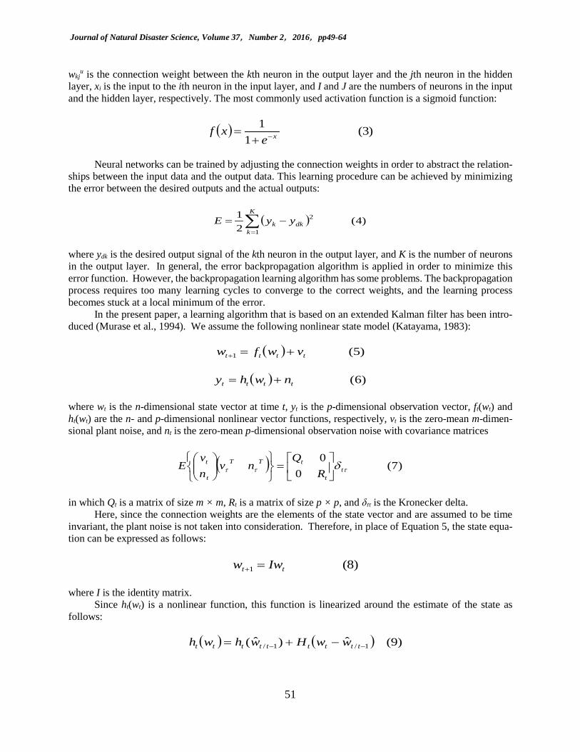
wkju is the connection weight between the kth neuron in the output layer and the jth neuron in the hidden

layer, xi is the input to the ith neuron in the input layer, and I and J are the numbers of neurons in the input and the hidden layer, respectively. The most commonly used activation function is a sigmoid function:

( ) )3(1

1xe

xf −+=

Neural networks can be trained by adjusting the connection weights in order to abstract the relation-

ships between the input data and the output data. This learning procedure can be achieved by minimizing the error between the desired outputs and the actual outputs:

( )∑=

−=K

kdkk yyE

1

2 )4(21

where ydk is the desired output signal of the kth neuron in the output layer, and K is the number of neurons in the output layer. In general, the error backpropagation algorithm is applied in order to minimize this error function. However, the backpropagation learning algorithm has some problems. The backpropagation process requires too many learning cycles to converge to the correct weights, and the learning process becomes stuck at a local minimum of the error.

In the present paper, a learning algorithm that is based on an extended Kalman filter has been intro-duced (Murase et al., 1994). We assume the following nonlinear state model (Katayama, 1983):

( ) )5(1 tttt vwfw +=+

( ) )6(tttt nwhy +=

where wt is the n-dimensional state vector at time t, yt is the p-dimensional observation vector, ft(wt) and ht(wt) are the n- and p-dimensional nonlinear vector functions, respectively, vt is the zero-mean m-dimen-sional plant noise, and nt is the zero-mean p-dimensional observation noise with covariance matrices

( ) )7(0

0τττ δ t

t

tTT

t

t

RQ

nvnv

E

=

in which Qt is a matrix of size m × m, Rt is a matrix of size p × p, and δtτ is the Kronecker delta.

Here, since the connection weights are the elements of the state vector and are assumed to be time invariant, the plant noise is not taken into consideration. Therefore, in place of Equation 5, the state equa-tion can be expressed as follows:

)8(1 tt Iww =+

where I is the identity matrix.

Since ht(wt) is a nonlinear function, this function is linearized around the estimate of the state as follows:

( ) ( ) )9(ˆ)ˆ( 1/1/ −− −+= ttttttttt wwHwhwh

M.HORII, T.HAYAMI

52

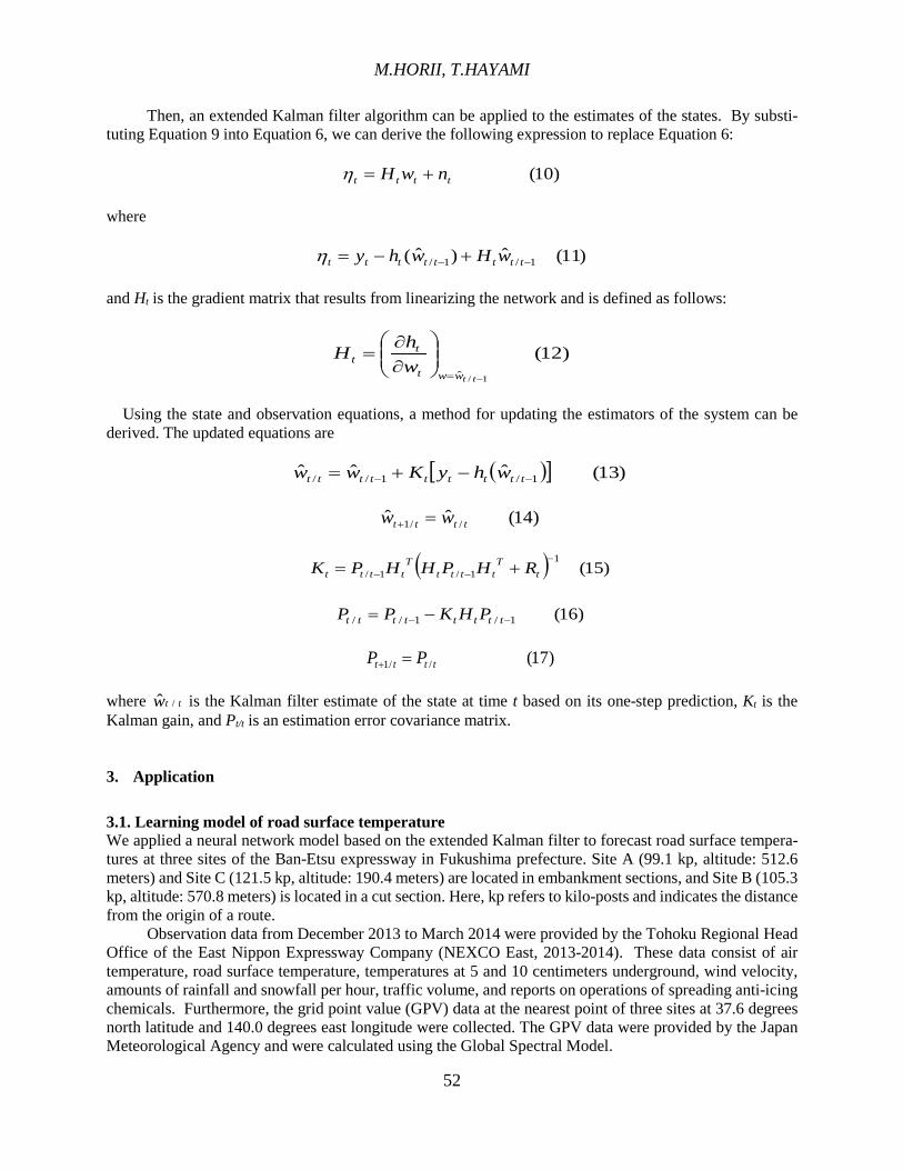
Then, an extended Kalman filter algorithm can be applied to the estimates of the states. By substi-tuting Equation 9 into Equation 6, we can derive the following expression to replace Equation 6:

)10(tttt nwH +=η

where

)11(ˆ)ˆ( 1/1/ −− +−= tttttttt wHwhyη

and Ht is the gradient matrix that results from linearizing the network and is defined as follows:

)12(1/ˆ −=

∂∂

=ttwwt

tt w

hH

Using the state and observation equations, a method for updating the estimators of the system can be

derived. The updated equations are

( )[ ] )13(ˆˆˆ 1/1// −− −+= ttttttttt whyKww

)14(ˆˆ //1 tttt ww =+

( ) )15(1

1/1/−

−− += tT

ttttT

tttt RHPHHPK

)16(1/1// −− −= tttttttt PHKPP

)17(//1 tttt PP =+

where is the Kalman filter estimate of the state at time t based on its one-step prediction, Kt is the Kalman gain, and Pt/t is an estimation error covariance matrix. 3. Application

3.1. Learning model of road surface temperature We applied a neural network model based on the extended Kalman filter to forecast road surface tempera-tures at three sites of the Ban-Etsu expressway in Fukushima prefecture. Site A (99.1 kp, altitude: 512.6 meters) and Site C (121.5 kp, altitude: 190.4 meters) are located in embankment sections, and Site B (105.3 kp, altitude: 570.8 meters) is located in a cut section. Here, kp refers to kilo-posts and indicates the distance from the origin of a route.

Observation data from December 2013 to March 2014 were provided by the Tohoku Regional Head Office of the East Nippon Expressway Company (NEXCO East, 2013-2014). These data consist of air temperature, road surface temperature, temperatures at 5 and 10 centimeters underground, wind velocity, amounts of rainfall and snowfall per hour, traffic volume, and reports on operations of spreading anti-icing chemicals. Furthermore, the grid point value (GPV) data at the nearest point of three sites at 37.6 degrees north latitude and 140.0 degrees east longitude were collected. The GPV data were provided by the Japan Meteorological Agency and were calculated using the Global Spectral Model.

ttw /ˆ


53

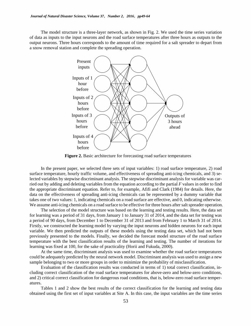
The model structure is a three-layer network, as shown in Fig. 2. We used the time series variation of data as inputs to the input neurons and the road surface temperatures after three hours as outputs to the output neurons. Three hours corresponds to the amount of time required for a salt spreader to depart from a snow removal station and complete the spreading operation.

Present inputs

Inputs of 1 hour

before

Inputs of 2 hours before



Outputs of 3 hours ahead

Figure 2. Basic architecture for forecasting road surface temperatures

In the present paper, we selected three sets of input variables: 1) road surface temperature, 2) road

surface temperature, hourly traffic volume, and effectiveness of spreading anti-icing chemicals, and 3) se-lected variables by stepwise discriminant analysis. The stepwise discriminant analysis for variable was car-ried out by adding and deleting variables from the equation according to the partial F values in order to find the appropriate discriminant equation. Refer to, for example, Afifi and Clark (1984) for details. Here, the data on the effectiveness of spreading anti-icing chemicals can be represented by a dummy variable that takes one of two values: 1, indicating chemicals on a road surface are effective, and 0, indicating otherwise. We assume anti-icing chemicals on a road surface to be effective for three hours after salt spreader operation.

The selection of the model structure was based on the learning and testing results. Here, the data set for learning was a period of 31 days, from January 1 to January 31 of 2014, and the data set for testing was a period of 90 days, from December 1 to December 31 of 2013 and from February 1 to March 31 of 2014. Firstly, we constructed the learning model by varying the input neurons and hidden neurons for each input variable. We then predicted the outputs of these models using the testing data set, which had not been previously presented to the models. Finally, we decided the forecast model structure of the road surface temperature with the best classification results of the learning and testing. The number of iterations for learning was fixed at 100, for the sake of practicality (Horii and Fukuda, 2000).

At the same time, discriminant analysis was used to examine whether the road surface temperatures could be adequately predicted by the neural network model. Discriminant analysis was used to assign a new sample belonging to two or more groups in order to minimize the probability of misclassification.

Evaluation of the classification results was conducted in terms of 1) total correct classification, in-cluding correct classification of the road surface temperatures for above-zero and below-zero conditions, and 2) critical correct classification for dangerous road conditions, that is, below-zero road surface temper-atures.

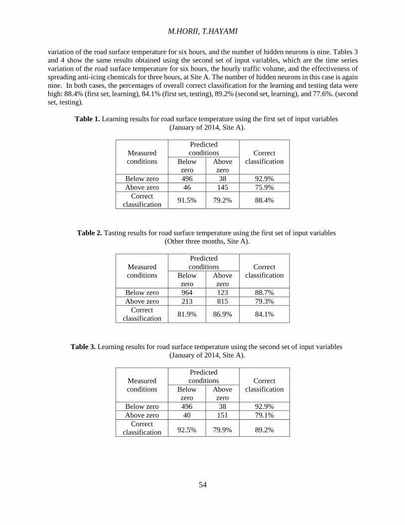
Tables 1 and 2 show the best results of the correct classification for the learning and testing data obtained using the first set of input variables at Site A. In this case, the input variables are the time series

M.HORII, T.HAYAMI

54

variation of the road surface temperature for six hours, and the number of hidden neurons is nine. Tables 3 and 4 show the same results obtained using the second set of input variables, which are the time series variation of the road surface temperature for six hours, the hourly traffic volume, and the effectiveness of spreading anti-icing chemicals for three hours, at Site A. The number of hidden neurons in this case is again nine. In both cases, the percentages of overall correct classification for the learning and testing data were high: 88.4% (first set, learning), 84.1% (first set, testing), 89.2% (second set, learning), and 77.6%. (second set, testing).

Table 1. Learning results for road surface temperature using the first set of input variables

(January of 2014, Site A).

Measured conditions

Predicted conditions Correct

classification Below zero

Above zero

Below zero 496 38 92.9% Above zero 46 145 75.9%

Correct classification 91.5% 79.2% 88.4%

Table 2. Tasting results for road surface temperature using the first set of input variables (Other three months, Site A).

Measured conditions



Above zero



Table 3. Learning results for road surface temperature using the second set of input variables (January of 2014, Site A).

Measured conditions



Above zero




55

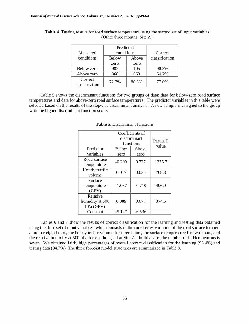
Table 4. Tasting results for road surface temperature using the second set of input variables (Other three months, Site A).

Measured conditions



Above zero



Table 5 shows the discriminant functions for two groups of data: data for below-zero road surface

temperatures and data for above-zero road surface temperatures. The predictor variables in this table were selected based on the results of the stepwise discriminant analysis. A new sample is assigned to the group with the higher discriminant function score.

Table 5. Discriminant functions

Predictor variables

Coefficients of discriminant

functions Partial F value Below

zero Above zero

Road surface temperature -0.209 0.727 1275.7

Hourly traffic volume 0.017 0.030 708.3

Surface temperature

(GPV) -1.037 -0.710 496.0

Relative humidity at 500

hPa (GPV) 0.089 0.077 374.5

Constant -5.127 -6.536

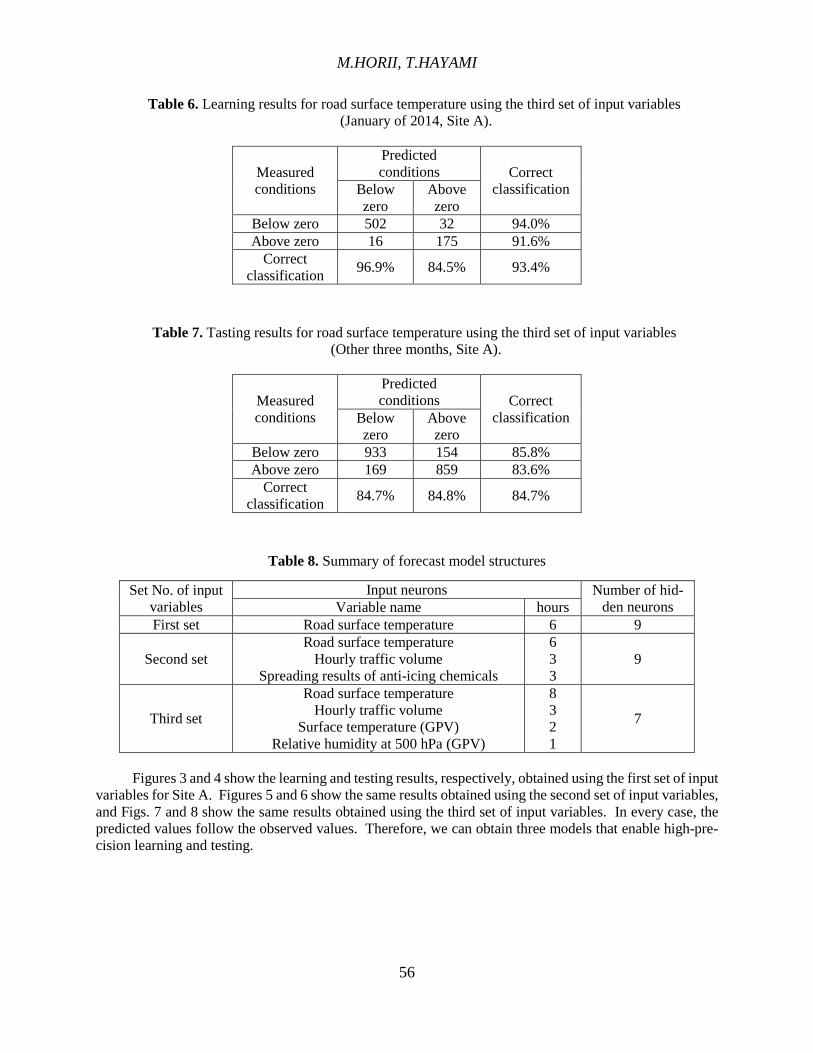
Tables 6 and 7 show the results of correct classification for the learning and testing data obtained using the third set of input variables, which consists of the time series variation of the road surface temper-ature for eight hours, the hourly traffic volume for three hours, the surface temperature for two hours, and the relative humidity at 500 hPa for one hour, all at Site A. In this case, the number of hidden neurons is seven. We obtained fairly high percentages of overall correct classification for the learning (93.4%) and testing data (84.7%). The three forecast model structures are summarized in Table 8.

M.HORII, T.HAYAMI

56

Table 6. Learning results for road surface temperature using the third set of input variables (January of 2014, Site A).

Measured conditions



Above zero



Table 7. Tasting results for road surface temperature using the third set of input variables (Other three months, Site A).

Measured conditions



Above zero



Table 8. Summary of forecast model structures

Set No. of input variables

Input neurons Number of hid-den neurons Variable name hours

First set Road surface temperature 6 9

Second set Road surface temperature

Hourly traffic volume Spreading results of anti-icing chemicals

6 3 3

9

Third set

Road surface temperature Hourly traffic volume

Surface temperature (GPV) Relative humidity at 500 hPa (GPV)

8 3 2 1

7

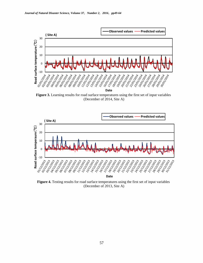
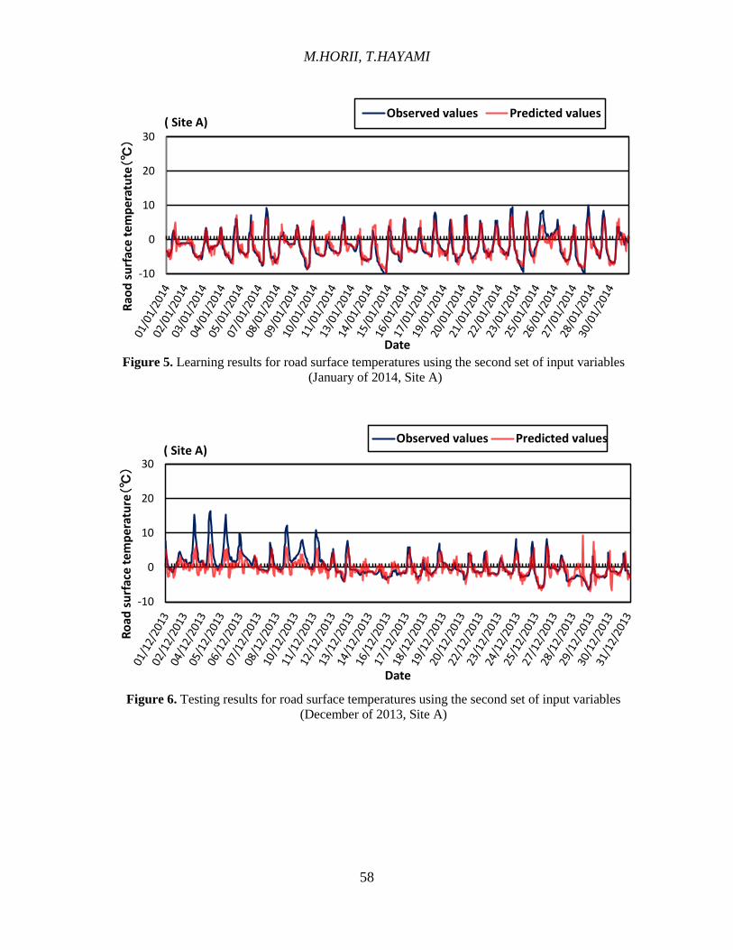
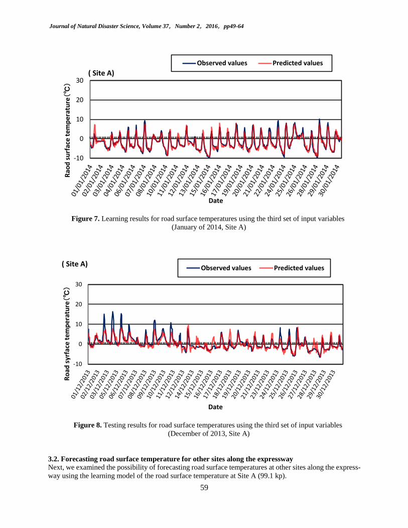
Figures 3 and 4 show the learning and testing results, respectively, obtained using the first set of input

variables for Site A. Figures 5 and 6 show the same results obtained using the second set of input variables, and Figs. 7 and 8 show the same results obtained using the third set of input variables. In every case, the predicted values follow the observed values. Therefore, we can obtain three models that enable high-pre-cision learning and testing.


57

Figure 3. Learning results for road surface temperatures using the first set of input variables

(December of 2014, Site A)

Figure 4. Testing results for road surface temperatures using the first set of input variables


-10

0

10

20

30Ro

ad su

rfac

e te

mpe

ratu

re（℃

）

Date

Observed values Predicted values( Site A)

-10

0

10

20

30

Road

surf

ace

tem

pera

ure（

℃）

Date


M.HORII, T.HAYAMI

58

Figure 5. Learning results for road surface temperatures using the second set of input variables

(January of 2014, Site A)

Figure 6. Testing results for road surface temperatures using the second set of input variables


-10

0

10

20

30Ra

od su

rfac

e te

mpe

ratu

te（℃

）

Date


-10

0

10

20

30

Road

surf

ace

tem

pera

ture（℃

）

Date



59

Figure 7. Learning results for road surface temperatures using the third set of input variables (January of 2014, Site A)

Figure 8. Testing results for road surface temperatures using the third set of input variables (December of 2013, Site A)

3.2. Forecasting road surface temperature for other sites along the expressway Next, we examined the possibility of forecasting road surface temperatures at other sites along the express-way using the learning model of the road surface temperature at Site A (99.1 kp).

-10

0

10

20

30

Raod

surf

ace

tem

pera

ture（℃

）

Date


-10

0

10

20

30

Road

syrf

ace

tem

pera

ture（℃

）

Date


M.HORII, T.HAYAMI

60

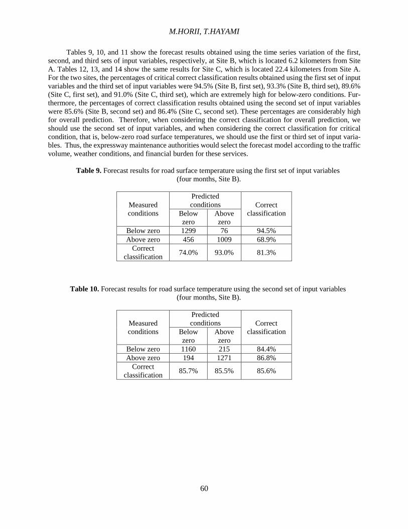
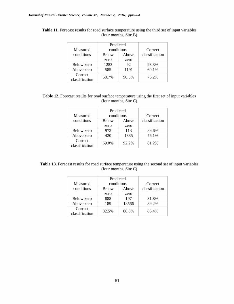
Tables 9, 10, and 11 show the forecast results obtained using the time series variation of the first, second, and third sets of input variables, respectively, at Site B, which is located 6.2 kilometers from Site A. Tables 12, 13, and 14 show the same results for Site C, which is located 22.4 kilometers from Site A. For the two sites, the percentages of critical correct classification results obtained using the first set of input variables and the third set of input variables were 94.5% (Site B, first set), 93.3% (Site B, third set), 89.6% (Site C, first set), and 91.0% (Site C, third set), which are extremely high for below-zero conditions. Fur-thermore, the percentages of correct classification results obtained using the second set of input variables were 85.6% (Site B, second set) and 86.4% (Site C, second set). These percentages are considerably high for overall prediction. Therefore, when considering the correct classification for overall prediction, we should use the second set of input variables, and when considering the correct classification for critical condition, that is, below-zero road surface temperatures, we should use the first or third set of input varia-bles. Thus, the expressway maintenance authorities would select the forecast model according to the traffic volume, weather conditions, and financial burden for these services.

Table 9. Forecast results for road surface temperature using the first set of input variables (four months, Site B).

Measured conditions



Above zero



Table 10. Forecast results for road surface temperature using the second set of input variables (four months, Site B).

Measured conditions



Above zero




61

Table 11. Forecast results for road surface temperature using the third set of input variables (four months, Site B).

Measured conditions



Above zero



Table 12. Forecast results for road surface temperature using the first set of input variables (four months, Site C).

Measured conditions



Above zero



Table 13. Forecast results for road surface temperature using the second set of input variables (four months, Site C).

Measured conditions



Above zero



M.HORII, T.HAYAMI

62

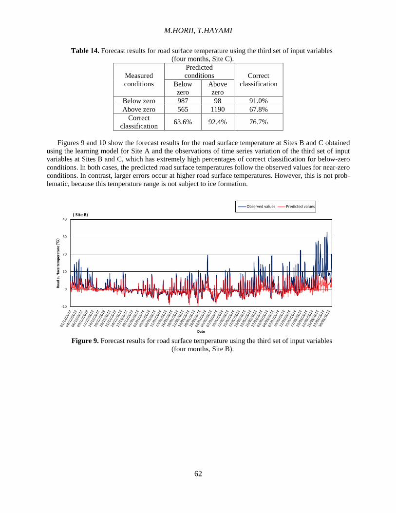
Table 14. Forecast results for road surface temperature using the third set of input variables (four months, Site C).

Measured conditions



Above zero



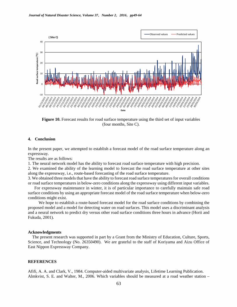
Figures 9 and 10 show the forecast results for the road surface temperature at Sites B and C obtained using the learning model for Site A and the observations of time series variation of the third set of input variables at Sites B and C, which has extremely high percentages of correct classification for below-zero conditions. In both cases, the predicted road surface temperatures follow the observed values for near-zero conditions. In contrast, larger errors occur at higher road surface temperatures. However, this is not prob-lematic, because this temperature range is not subject to ice formation.

Figure 9. Forecast results for road surface temperature using the third set of input variables

(four months, Site B).

-10

0

10

20

30

40

Road

surf

ace

tem

pera

ture（℃

）

Date

Observed values Predicted values

( Site B)


63

Figure 10. Forecast results for road surface temperature using the third set of input variables (four months, Site C).

4. Conclusion

In the present paper, we attempted to establish a forecast model of the road surface temperature along an expressway. The results are as follows: 1. The neural network model has the ability to forecast road surface temperature with high precision. 2. We examined the ability of the learning model to forecast the road surface temperature at other sites along the expressway, i.e., route-based forecasting of the road surface temperature. 3. We obtained three models that have the ability to forecast road surface temperatures for overall conditions or road surface temperatures in below-zero conditions along the expressway using different input variables. For expressway maintenance in winter, it is of particular importance to carefully maintain safe road surface conditions by using an appropriate forecast model of the road surface temperature when below-zero conditions might exist.

We hope to establish a route-based forecast model for the road surface conditions by combining the proposed model and a model for detecting water on road surfaces. This model uses a discriminant analysis and a neural network to predict dry versus other road surface conditions three hours in advance (Horii and Fukuda, 2001). Acknowledgments

The present research was supported in part by a Grant from the Ministry of Education, Culture, Sports, Science, and Technology (No. 26350490). We are grateful to the staff of Koriyama and Aizu Office of East Nippon Expressway Company. REFERENCES Afifi, A. A. and Clark, V., 1984. Computer-aided multivariate analysis, Lifetime Learning Publication. Almkvist, S. E. and Walter, M., 2006. Which variables should be measured at a road weather station –

-10

0

10

20

30

40

Road

surf

ace

tem

pera

ture（℃

）

Date

Observed values Predicted values( Site C)

M.HORII, T.HAYAMI

64

Artificial intelligence gives the answer, SIRWEC, 101-107. Horii, M. and Fukuda, T., 2000. Forecast model of road surface temperature in snowy areas using neural

network, Proceedings of the Fourth International Conference on Snow Engineering, 403-407. Horii, M. and Fukuda, T., 2001. Pavement ice prediction system in winter maintenance, Journal of Materials,

Concrete Structures and Pavements, 669, 243-251. Horii, M., 2013. Forecast model of road surface temperature along national highway in snowy area, Journal

of Snow Engineering of Japan, 29 (1), 13-22. Horii, M. and Hayami, T., 2015. Forecast model of road surface temperature along expressway, Summaries

of JSSI & JSSE Joint Conf. on Snow and Ice Research, 99. Katayama, T., 1983. Applied Kalman Filter, Asakura Publishing Co., Ltd. Murase, H., Koyama, S., and Ishida, R., 1994. Kalman neuro computing by personal computer, Morikita

Publishing Co., Ltd. NEXCO East, 2013-2014. Meteorological and Traffic Survey Data. Rayer, P. J., 1987. The Meteorological Office forecast road surface temperature model, Meteorological

Magazine, 116, 180-191. Shao, J., Thornes, J. E., and Lister, P. J., 1993. Description and verification of a road ice prediction model,

Transportation Research Record, 1387, 216-222. Shao, J., 1998. Improving nowcasts of road surface temperature by a backpropagation neural network,

Weather and Forecasting, 13, 164-171. Suzuki, T., Amano, T., and Hirama, S., 1993. Research on new system for prediction freezing on road

surfaces, Report of Research Center of Japan Highway Public Corporation, Vol. 30, 179-190. Voldborg, H., 1993. On the prediction of road conditions by a combined road layer-atmospheric model in

winter, Transportation Research Record, 1387, 231-235.

Documents

Model for forecasting expressway surface temperature in ... · Journal of Natural Disaster Science, Volume 37，Number 2，2016，pp49-64 49 . Model for forecasting expressway surface