Model Construction: interpolation techniques

1392

Introduction

• There is no ideal DEM. – DEM generation techniques can not capture the full

complexity of a surface.– There is always a sampling problem and a

representation problem.• Continuous Surface Discrete Surface Continuous ⇒ ⇒

Surface.

Surface Characteristics

• Functional Surfaces:– Store a single z value for any given X,Y location.– Represent continuous surfaces.– Referred to as 2.5 dimensional surfaces.

• Solid Models:– True 3 dimensional models capable of storing multiple

Z values for any given (X, Y) location.– Capable of representing discontinuous surfaces.– Examples: Machine parts, highway structures,

buildings.

Surface Characteristics

• Surface Continuity:– Continuous Surface: If you approach a given X, Y

location on a functional surface from any direction, you will get the same Z value.

– Solid models are capable of storing more than one Z value for a given (X, Y) location (discontinuous surfaces).

Surface Characteristics• Surface Smoothness:

– In addition to being continuous, a smooth surface has the additional property that regardless of the direction from which you approach a given point on the surface, the surface normal is constant.

– Geologically young terrain have sharp ridges and valleys. In contrast, older terrain are smoothed by weathering forces.

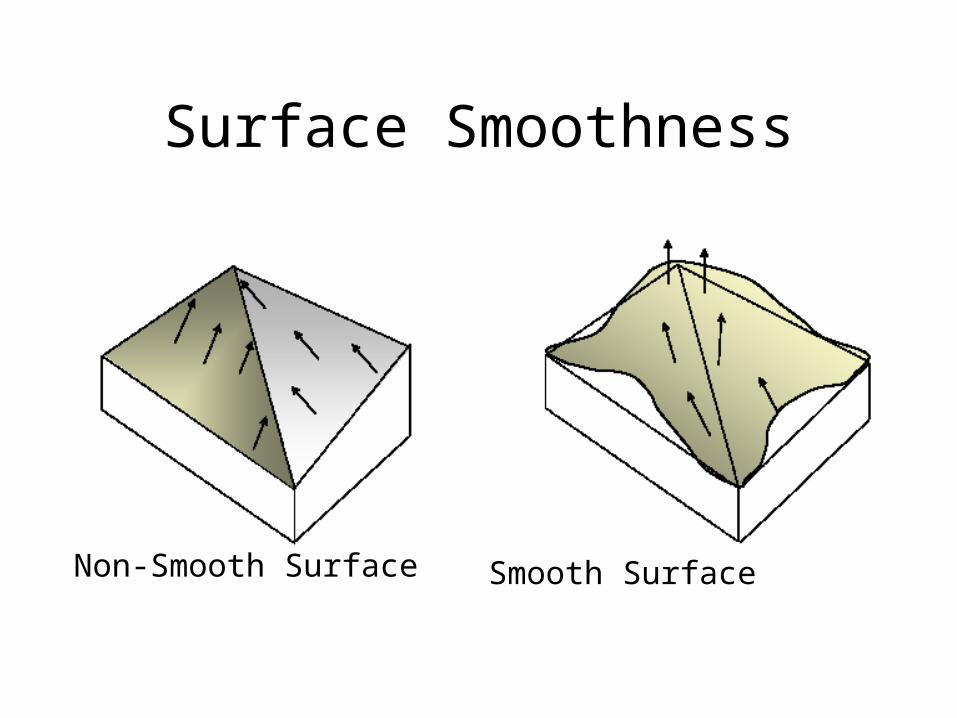
Surface Smoothness

Non-Smooth Surface Smooth Surface

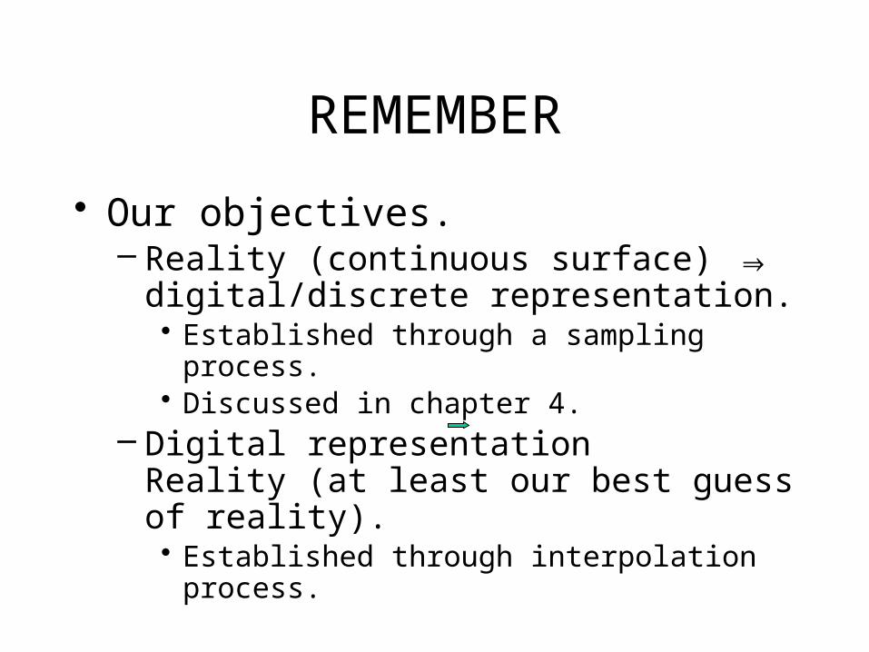
REMEMBER

• Our objectives.– Reality (continuous surface) digital/discrete ⇒

representation.• Established through a sampling process.• Discussed in chapter 4.

– Digital representation Reality (at least our best guess of reality).• Established through interpolation process.

Interpolation Vs. Extrapolation

• Interpolation:– The process of estimating the values of an attribute

(e.g., elevation) at internal unsampled sites using measurements made at reference points.

– The interpolation point lies within the range defined by the reference points.

• Extrapolation:– The process of predicting the values of an attribute

(e.g., elevation) at external unsampled sites using measurements made at reference points.

– The extrapolation point lies outside the range defined by the reference points.

Interpolation Vs. Extrapolation

•Reference Points.•Interpolation Point.•Extrapolation Point.

Measured Height

Derived Height

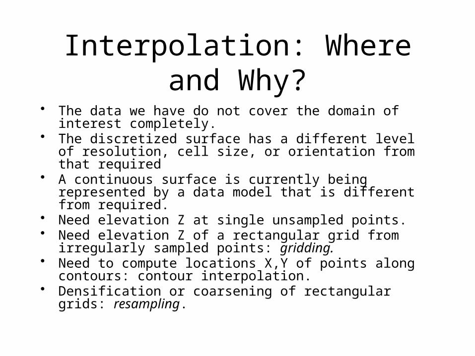
Interpolation: Where and Why?

• The data we have do not cover the domain of interest completely.• The discretized surface has a different level of resolution, cell size, or

orientation from that required• A continuous surface is currently being represented by a data model

that is different from required.• Need elevation Z at single unsampled points.• Need elevation Z of a rectangular grid from irregularly sampled

points: gridding.• Need to compute locations X,Y of points along contours: contour

interpolation.• Densification or coarsening of rectangular grids: resampling.

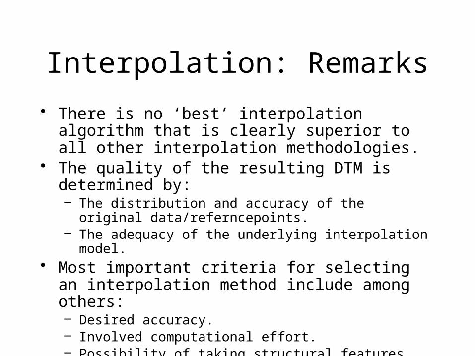
Interpolation: Remarks

• There is no ‘best’ interpolation algorithm that is clearly superior to all other interpolation methodologies.

• The quality of the resulting DTM is determined by:– The distribution and accuracy of the original data/referncepoints.– The adequacy of the underlying interpolation model.

• Most important criteria for selecting an interpolation method include among others:– Desired accuracy.– Involved computational effort.– Possibility of taking structural features into account.– Adaptability to the varying characteristics of the terrain.

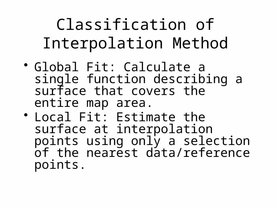
Classification of Interpolation Method

• Global Fit: Calculate a single function describing a surface that covers the entire map area.

• Local Fit: Estimate the surface at interpolation points using only a selection of the nearest data/reference points.

Global Interpolation

Trend Surface Analysis (TSA)

• A global fit interpolation method, which has the following characteristics:– Elevations are approximated by a polynomial

expansion.– The coefficients of the polynomial function are

determined through a least squares adjustment.– Each original observation is considered to be the sum

of a deterministic polynomial function of the geographic/planimetric coordinates plus a random error.

– Because of the least-squares fitting procedure, no other polynomial equation of the same degree can provide a better approximation of the data.

TSA: Concept

• Observed data points are assumed to be the superposition of two components:– Regional/trend: Low frequency component of the

surface (borrowed from Fourier Analysis). – Local fluctuations: High frequency component of the

surface.• The optimum trend, or linear function, must

minimize the squared sum of deviations (local fluctuations) between the original surface and its trend.

Trend Surfaces in 3-D

First Order Trend Surface

• A first order linear trend surface equation has the form:

•Question: How can we determine the coefficients e(x,y)

so that e is minimised?

First Order Trend Surface• Observation Equations:

•Normal Equations:

First Order Trend Surface

• Normal Equations:

Normal Equations

Trend Surface Analysis

• Second Order Polynomial Trend Surface:

•Third Order Polynomial Trend Surface:

Trend Surface Analysis

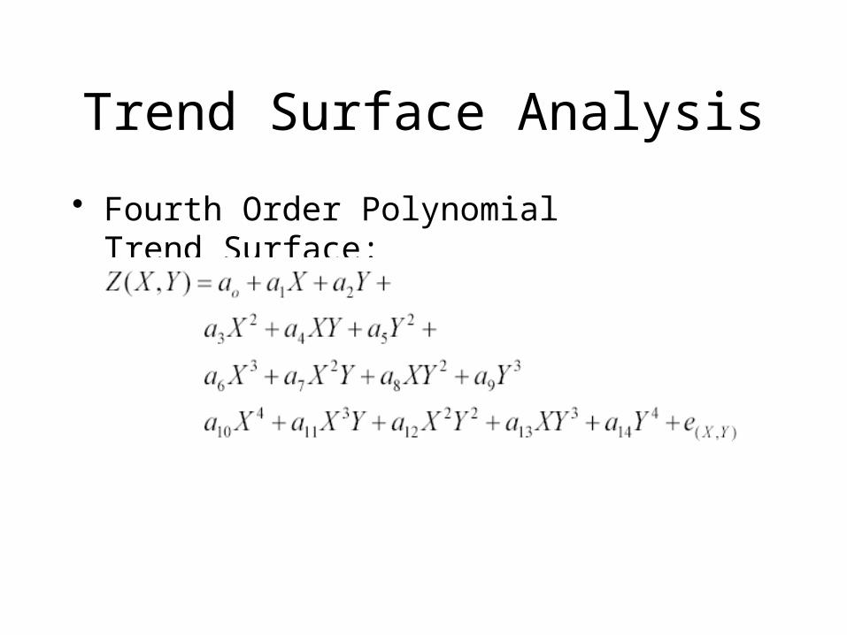
• Fourth Order Polynomial Trend Surface:

Trend Surface Analysis• Fifth Order Polynomial Surface:

Order Polynomial Surface:

TSA: Example

• Given: irregularly distributed set of reference points– Fit a first, second and third order trend surfaces through the given

points.– Calculate the estimated elevations and the corresponding residuals

for the given reference points.– Calculate the percentage of goodness of fit of the regression.

TSA: Example (Original Surface)

TSA: Example (Original Surface)

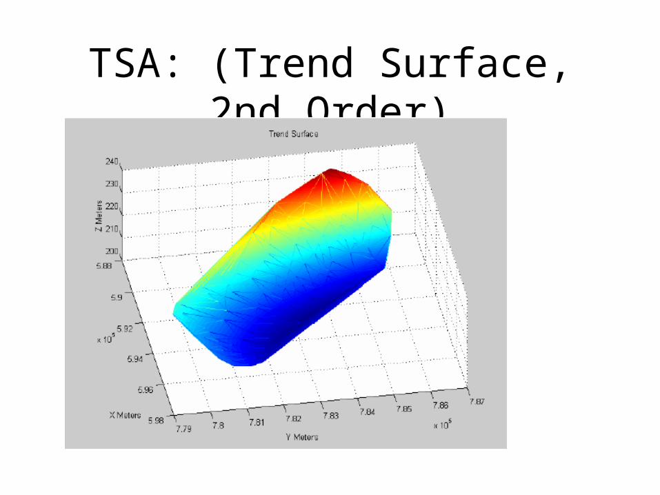
TSA: (Trend Surface, 2nd Order)

TSA: (Original/Trend Surfaces , 2nd Order)

TSA: (Residual Plot , 2nd Order)

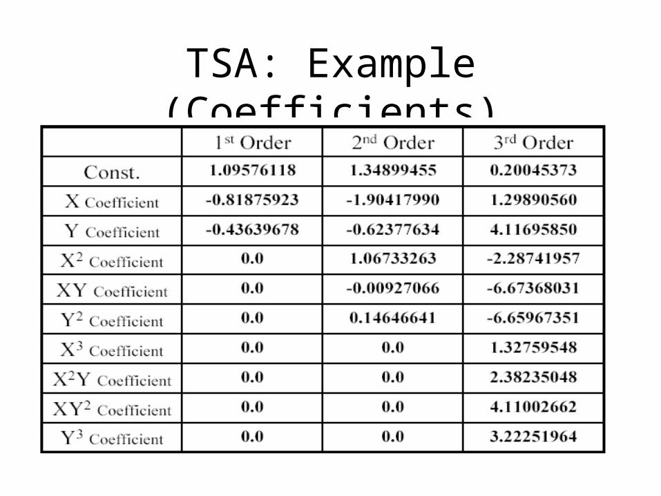
TSA: Example (Coefficients)

TSA: Remarks

• The coefficients of the design matrix (A) are proportional to the planimetric coordinates of the reference points.

• When dealing with large numbers, numerical instability is expected.

• Solution:– Option (1): Shift the coordinate system to the centroid

of the area of interest.– Option (2): Normalize the coordinates to the range

(0:1).

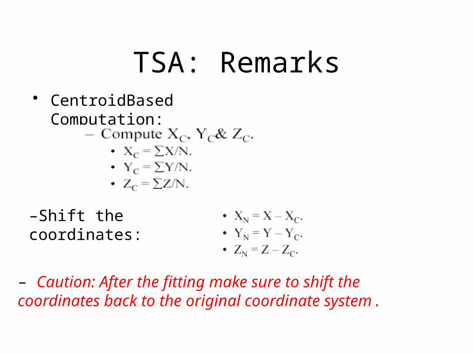
TSA: Remarks• CentroidBased Computation:

–Shift the coordinates:

– Caution: After the fitting make sure to shift the coordinates back to the original coordinate system.

TSA: Remarks

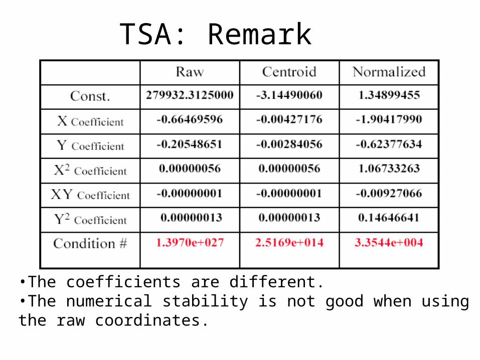
TSA: Remark

•The coefficients are different.•The numerical stability is not good when using the raw coordinates.

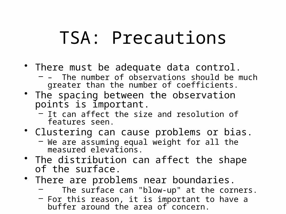
TSA: Precautions

• There must be adequate data control. – – The number of observations should be much greater than

the number of coefficients.• The spacing between the observation points is important.

– It can affect the size and resolution of features seen. • Clustering can cause problems or bias.

– We are assuming equal weight for all the measured elevations.• The distribution can affect the shape of the surface.• There are problems near boundaries.

– The surface can "blow-up" at the corners. – For this reason, it is important to have a buffer around the area of

concern.

TSA: Advantages

• Unique surface generated.• Easy to program.• Same surface estimated regardless of orientation

of reference geographic.• Calculation time for low order surfaces is low.• If the raw data are statistical in nature, with

perhaps more than one value at an observation point, trend surfaces provide statistically optimal estimates of a linear model that describes their spatial distribution.

TSA: Disadvantages

• Statistical assumptions of the model are rarely met in practice.

• Local anomalies can not be seen on contour maps of low order polynomials (but can be seen on contour maps of residuals).

• The surfaces are highly susceptible to edge effects.• Difficulty to describe a physical meaning to

complex and high order polynomial.

Problems with Trend Surfaces

• Polynomial surface is too simple in comparison to most natural surfaces.

• Difficulty in extrapolating beyond the area of data control.– Prone to the generation of seriously exaggerated

estimates.• Computational difficulties may be encountered if a

very high order polynomial trend surface is fitted.• The matrix solution may become unstable, or

rounding errors may result in erroneous trend surface coefficients.