Embed Size (px)
Citation preview
3-1 Department of Computer Science and Engineering
3 Interpolation Techniques
Chapter 3
Interpolation Techniques
3-2 Department of Computer Science and Engineering
3 Interpolation Techniques
Animation
Animator specified
interpolation
key frame
Algorithmically controlled
Physics-based
Behavioral
Data-driven
motion capture
Chapter 3
3-3 Department of Computer Science and Engineering
3 Interpolation Techniques
Motivation
Common problem: given a set of points
Smoothly (in time and space) move an
object through the set of points
Example additional temporal constraints:
From zero velocity at first point,
smoothly accelerate until time t1, hold a
constant velocity until time t2, then
smoothly decelerate to a stop at the last
point at time t3
Chapter 3
3-4 Department of Computer Science and Engineering
3 Interpolation Techniques
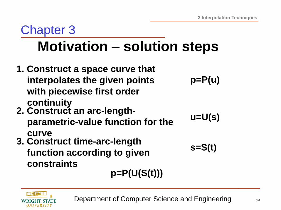
Motivation – solution steps
1. Construct a space curve that
interpolates the given points
with piecewise first order
continuity 2. Construct an arc-length-
parametric-value function for the
curve 3. Construct time-arc-length
function according to given
constraints
p=P(u)
u=U(s)
s=S(t)
p=P(U(S(t)))
Chapter 3
3-5 Department of Computer Science and Engineering
3 Interpolation Techniques
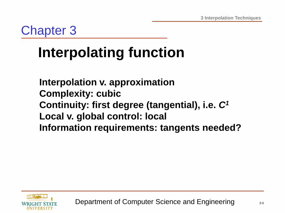
Interpolating function
Interpolation v. approximation
Complexity: cubic
Continuity: first degree (tangential), i.e. C1
Local v. global control: local
Information requirements: tangents needed?
Chapter 3
3-6 Department of Computer Science and Engineering
3 Interpolation Techniques
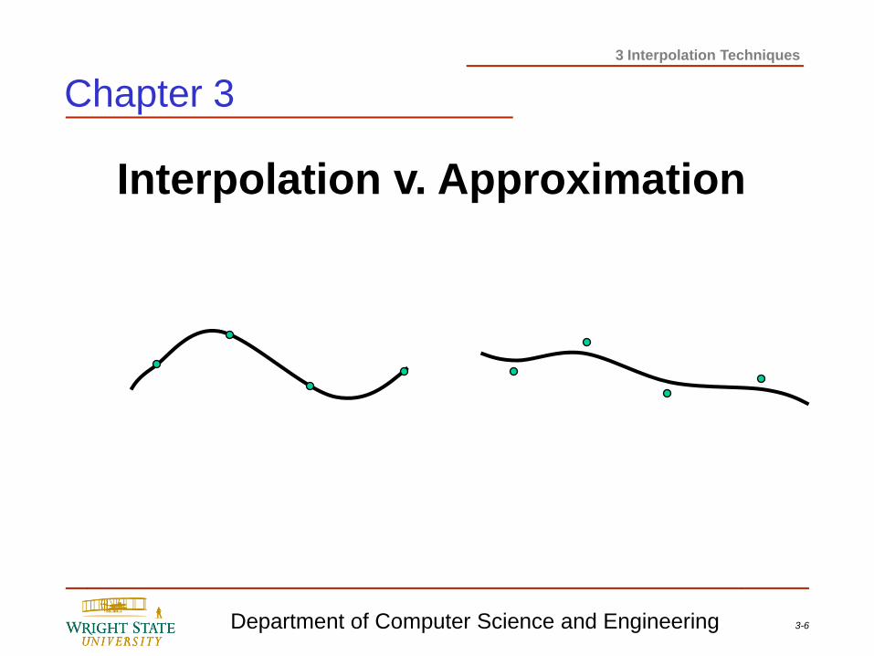
Interpolation v. Approximation
Chapter 3
3-7 Department of Computer Science and Engineering
3 Interpolation Techniques
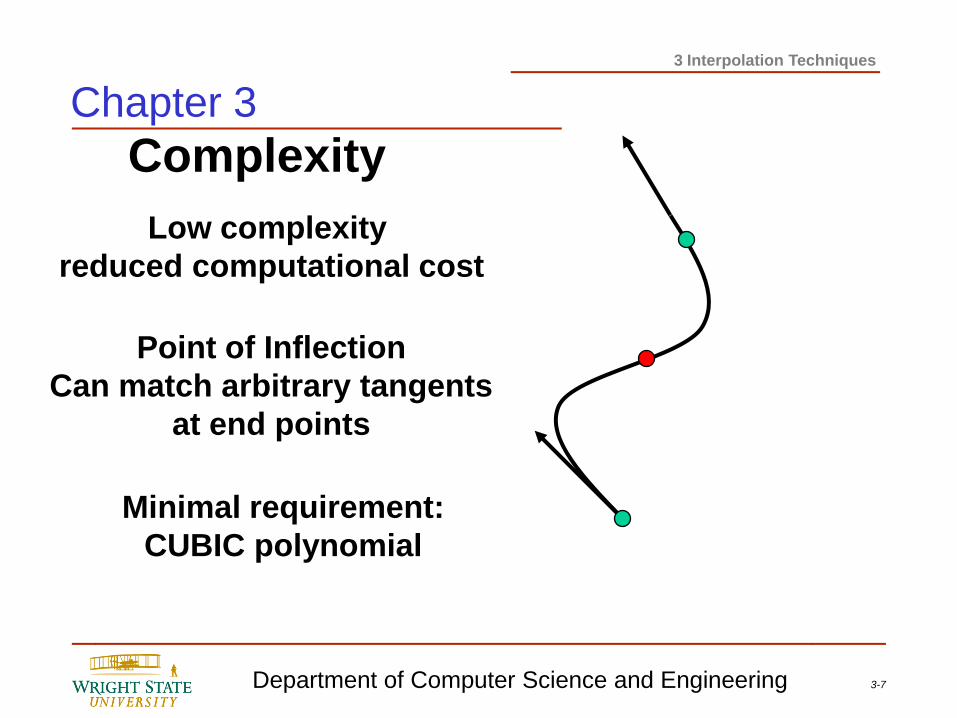
Complexity
Low complexity
reduced computational cost
Minimal requirement:
CUBIC polynomial
Point of Inflection
Can match arbitrary tangents
at end points
Chapter 3
3-8 Department of Computer Science and Engineering
3 Interpolation Techniques
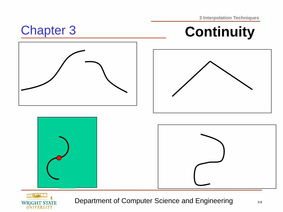
Continuity Chapter 3
3-9 Department of Computer Science and Engineering
3 Interpolation Techniques
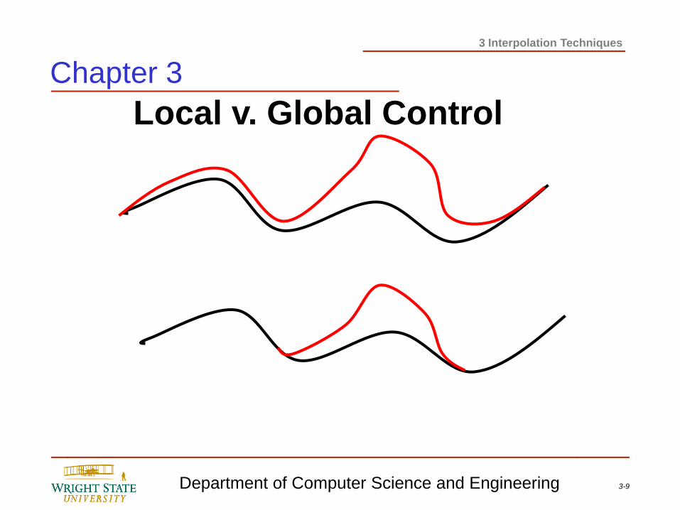
Local v. Global Control
Chapter 3
3-10 Department of Computer Science and Engineering
3 Interpolation Techniques
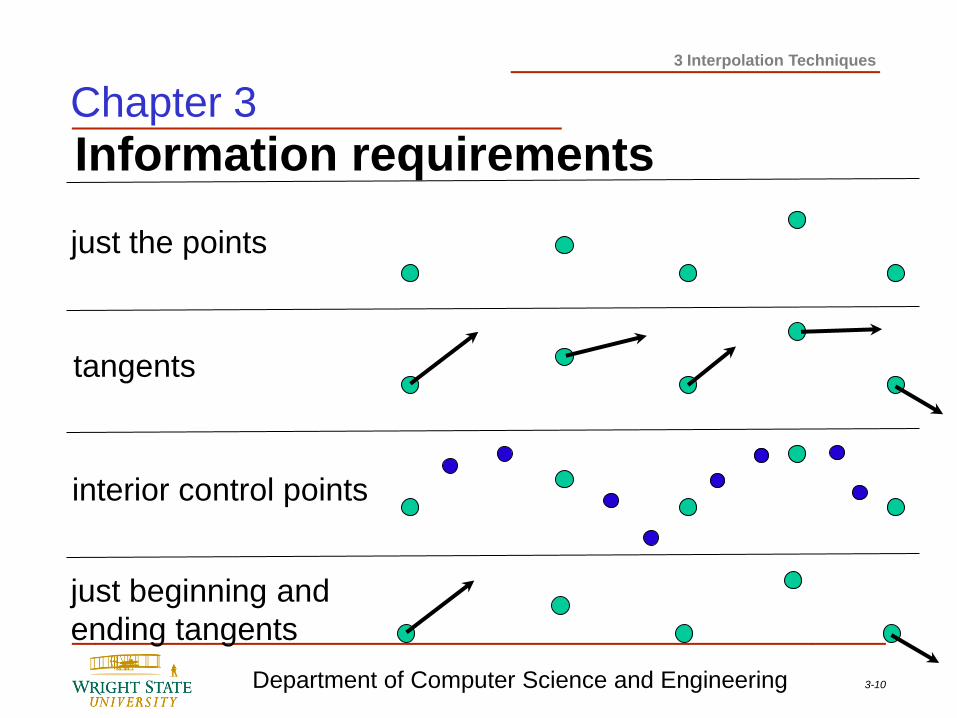
Information requirements
just the points
tangents
interior control points
just beginning and
ending tangents
Chapter 3
3-11 Department of Computer Science and Engineering
3 Interpolation Techniques
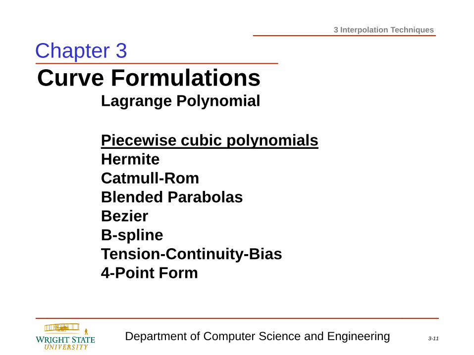
Curve Formulations
Piecewise cubic polynomials
Hermite
Catmull-Rom
Blended Parabolas
Bezier
B-spline
Tension-Continuity-Bias
4-Point Form
Lagrange Polynomial
Chapter 3
3-12 Department of Computer Science and Engineering
3 Interpolation Techniques
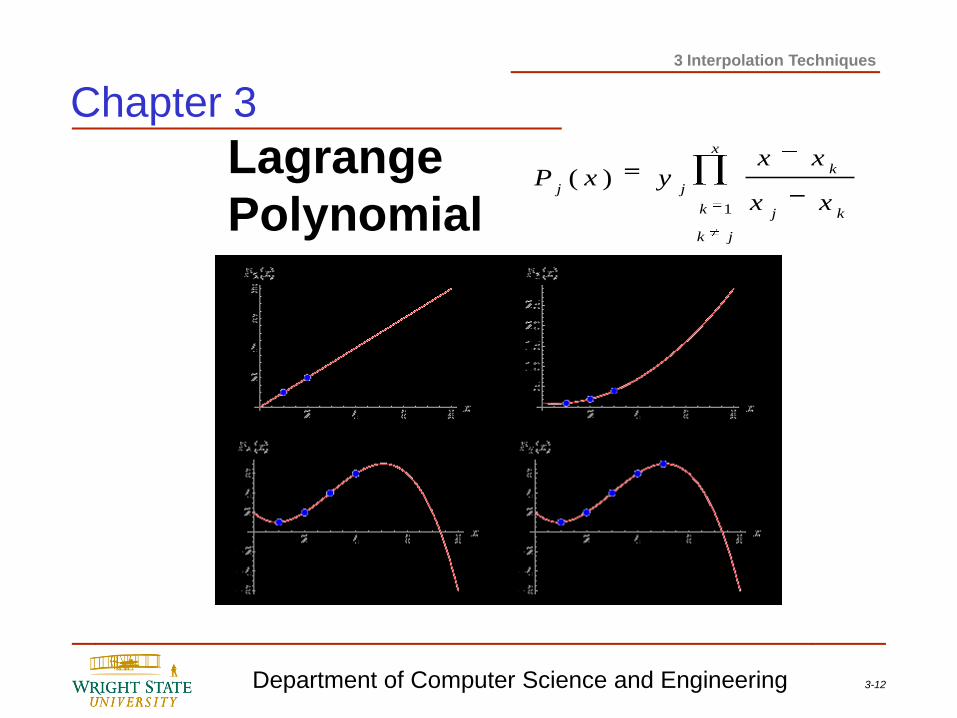
Lagrange
Polynomial
x
jk
k kj
k
jj
xx
xxyxP
1
)(
Chapter 3
3-13 Department of Computer Science and Engineering
3 Interpolation Techniques
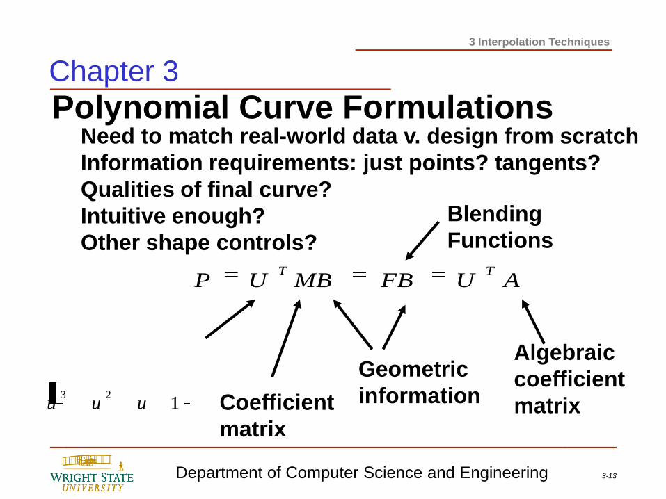
Polynomial Curve Formulations Need to match real-world data v. design from scratch
Information requirements: just points? tangents?
Qualities of final curve?
Intuitive enough?
Other shape controls?
AUFBMBUPTT
123
uuu
Geometric
information Coefficient
matrix
Blending
Functions
Algebraic
coefficient
matrix
Chapter 3
3-14 Department of Computer Science and Engineering
3 Interpolation Techniques
Chapter 3
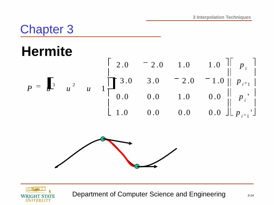
Hermite
'
'
0.00.00.00.1
0.00.10.00.0
0.10.20.30.3
0.10.10.20.2
1
1
123
i
i
i
i
p
p
p
p
uuuP
3-15 Department of Computer Science and Engineering
3 Interpolation Techniques
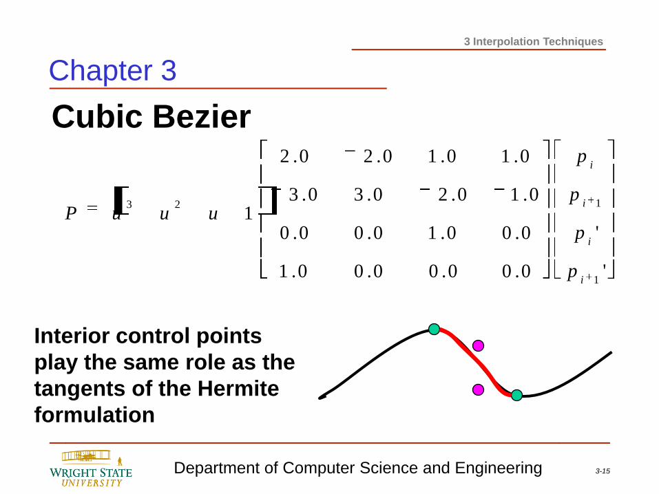
Cubic Bezier
'
'
0.00.00.00.1
0.00.10.00.0
0.10.20.30.3
0.10.10.20.2
1
1
123
i
i
i
i
p
p
p
p
uuuP
Interior control points
play the same role as the
tangents of the Hermite
formulation
Chapter 3
3-16 Department of Computer Science and Engineering
3 Interpolation Techniques
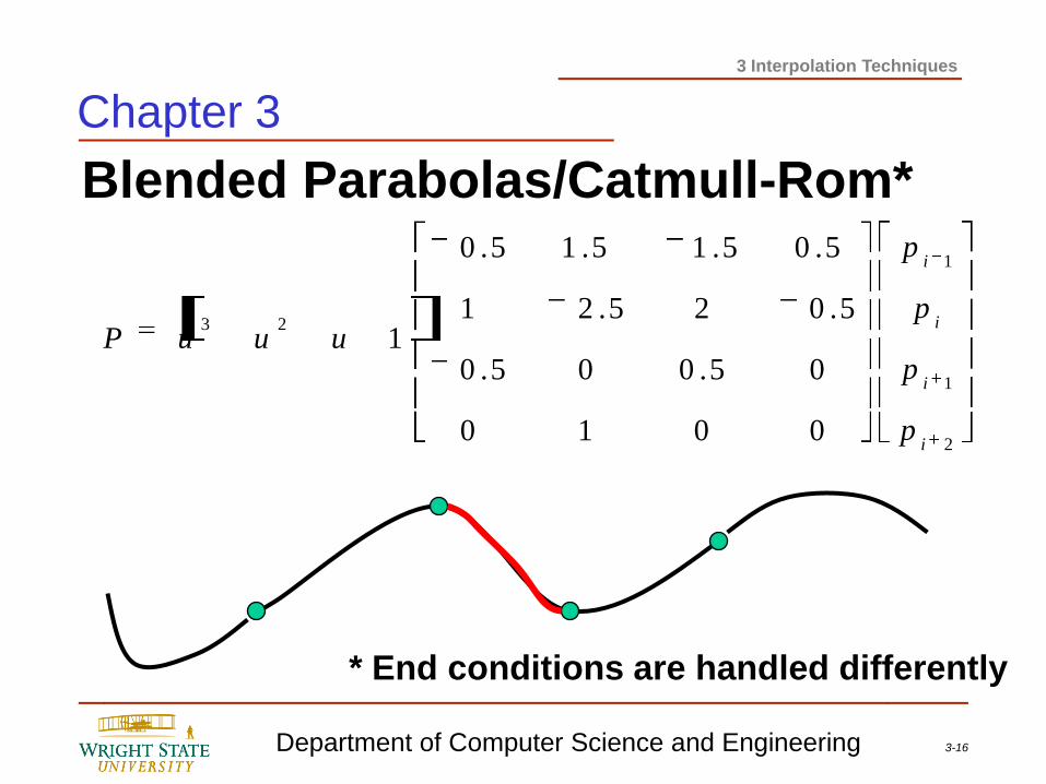
Blended Parabolas/Catmull-Rom*
2
1
1
23
0010
05.005.0
5.025.21
5.05.15.15.0
1
i
i
i
i
p
p
p
p
uuuP
* End conditions are handled differently
Chapter 3
3-17 Department of Computer Science and Engineering
3 Interpolation Techniques
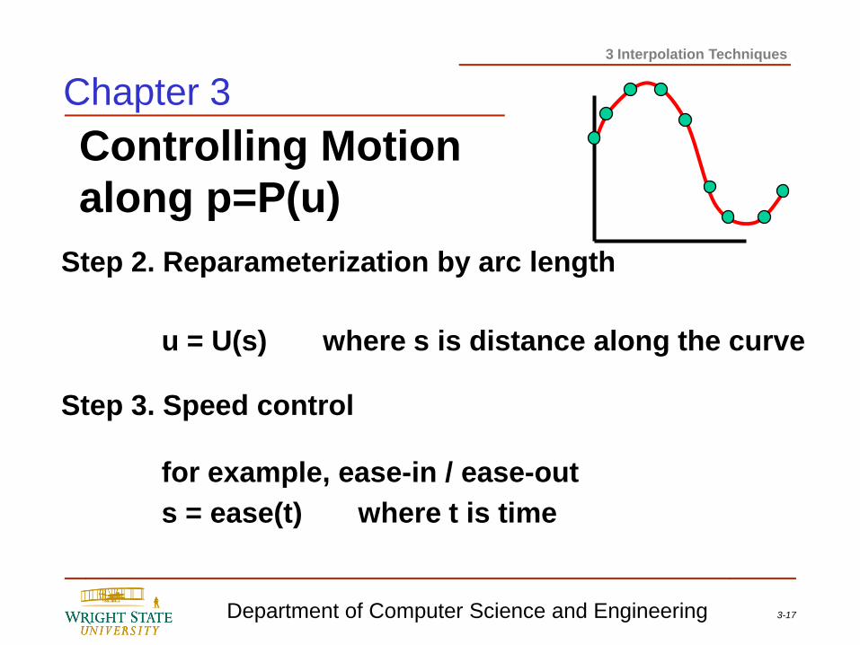
Controlling Motion
along p=P(u)
Step 2. Reparameterization by arc length
Step 3. Speed control
u = U(s) where s is distance along the curve
s = ease(t) where t is time
for example, ease-in / ease-out
Chapter 3
3-18 Department of Computer Science and Engineering
3 Interpolation Techniques
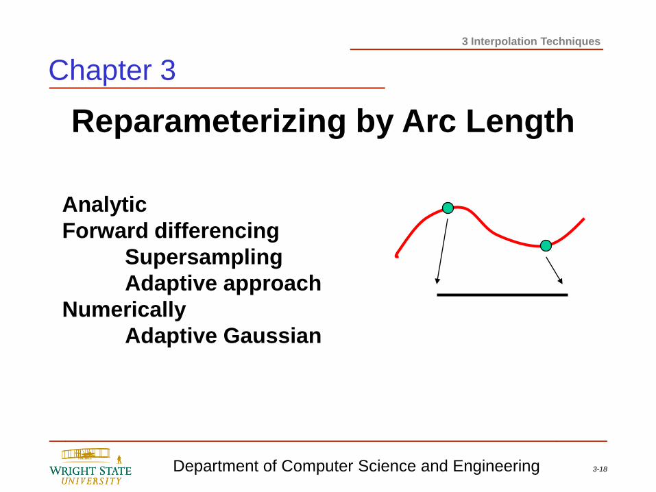
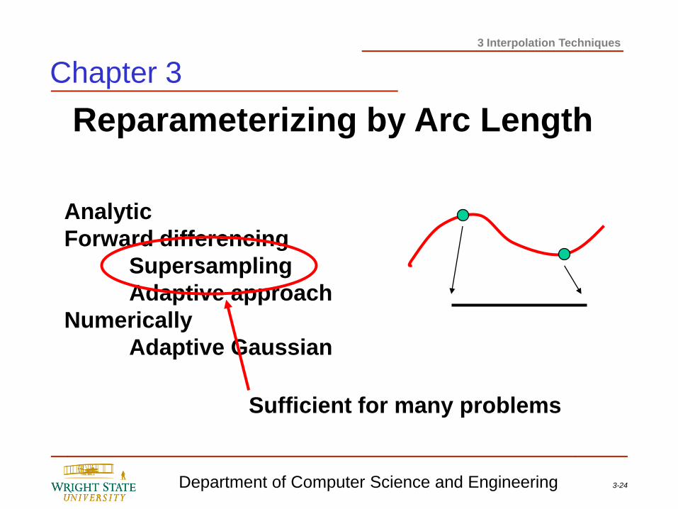
Reparameterizing by Arc Length
Analytic
Forward differencing
Supersampling
Adaptive approach
Numerically
Adaptive Gaussian
Chapter 3
3-19 Department of Computer Science and Engineering
3 Interpolation Techniques
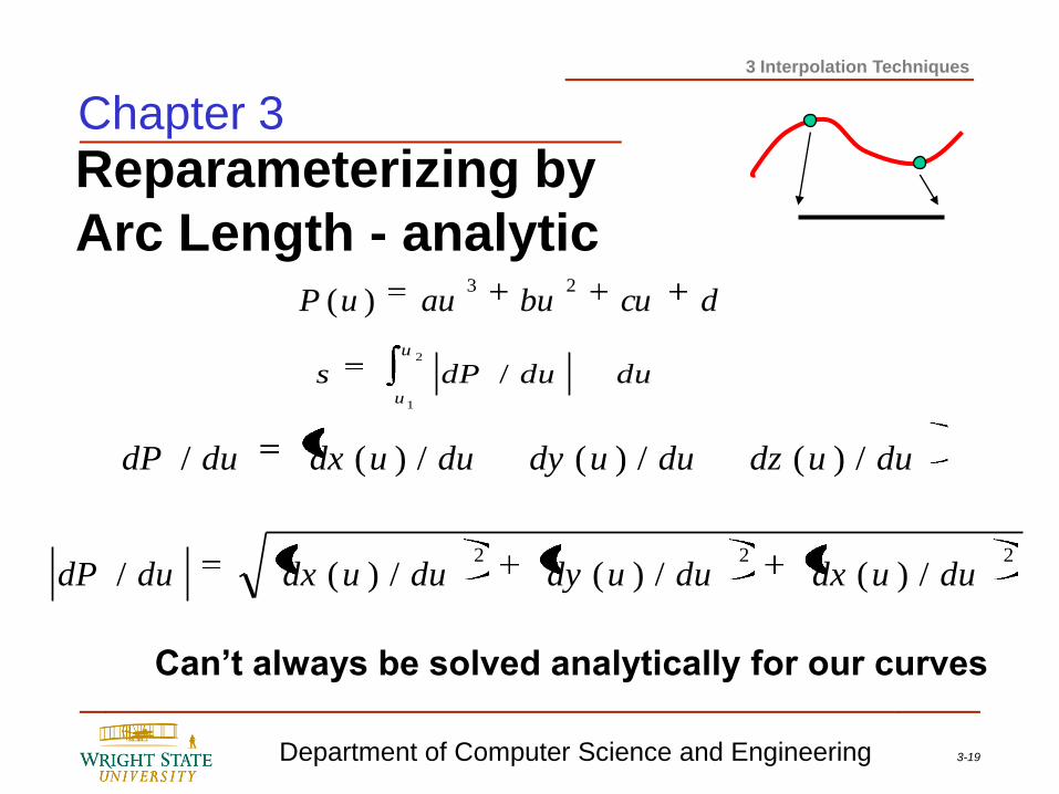
Reparameterizing by
Arc Length - analytic
2
1
/u
u
dududPs
duudzduudyduudxdudP /)(/)(/)(/
222
/)(/)(/)(/ duudxduudyduudxdudP
Can’t always be solved analytically for our curves
dcubuauuP23
)(
Chapter 3
3-20 Department of Computer Science and Engineering
3 Interpolation Techniques
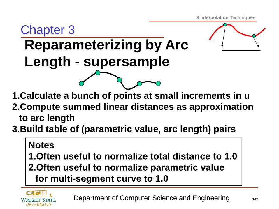
Reparameterizing by Arc
Length - supersample
1.Calculate a bunch of points at small increments in u
2.Compute summed linear distances as approximation
to arc length
3.Build table of (parametric value, arc length) pairs
Notes
1.Often useful to normalize total distance to 1.0
2.Often useful to normalize parametric value
for multi-segment curve to 1.0
Chapter 3
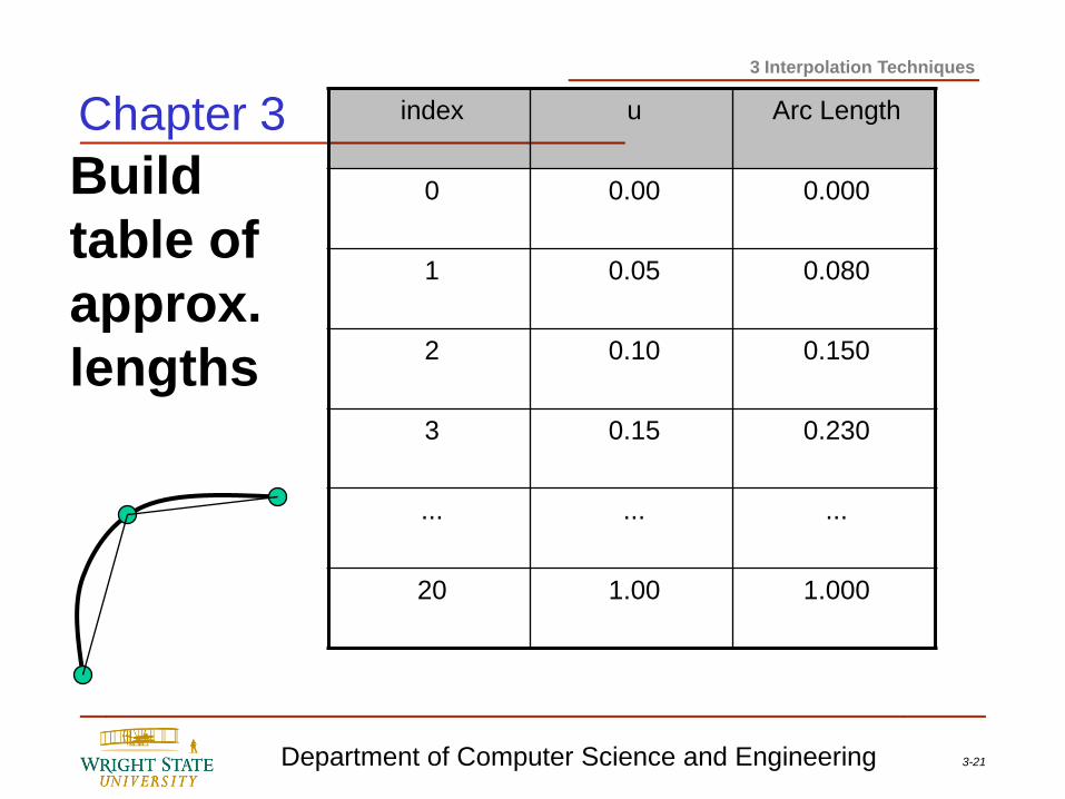
3-21 Department of Computer Science and Engineering
3 Interpolation Techniques
index u Arc Length
0 0.00 0.000
1 0.05 0.080
2 0.10 0.150
3 0.15 0.230
... ... ...
20 1.00 1.000
Build
table of
approx.
lengths
Chapter 3
3-22 Department of Computer Science and Engineering
3 Interpolation Techniques
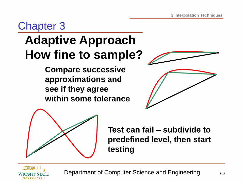
Adaptive Approach
How fine to sample? Compare successive
approximations and
see if they agree
within some tolerance
Test can fail – subdivide to
predefined level, then start
testing
Chapter 3
3-23 Department of Computer Science and Engineering
3 Interpolation Techniques
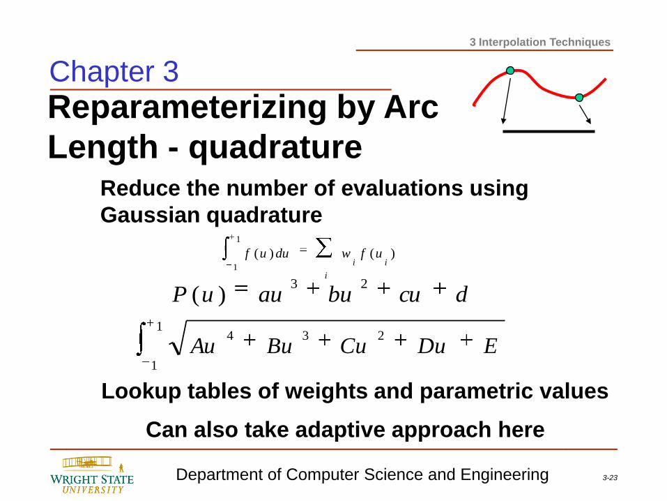
Reparameterizing by Arc
Length - quadrature
i
iiufwduuf )()(
1
1
Lookup tables of weights and parametric values
dcubuauuP23
)(
1
1
234EDuCuBuAu
Can also take adaptive approach here
Chapter 3
Reduce the number of evaluations using
Gaussian quadrature
3-24 Department of Computer Science and Engineering
3 Interpolation Techniques
Reparameterizing by Arc Length
Analytic
Forward differencing
Supersampling
Adaptive approach
Numerically
Adaptive Gaussian
Sufficient for many problems
Chapter 3
3-25 Department of Computer Science and Engineering
3 Interpolation Techniques
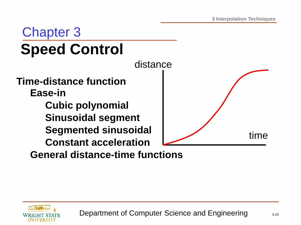
Speed Control
Time-distance function Ease-in
Cubic polynomial
Sinusoidal segment
Segmented sinusoidal
Constant acceleration
General distance-time functions
time
distance
Chapter 3
3-26 Department of Computer Science and Engineering
3 Interpolation Techniques
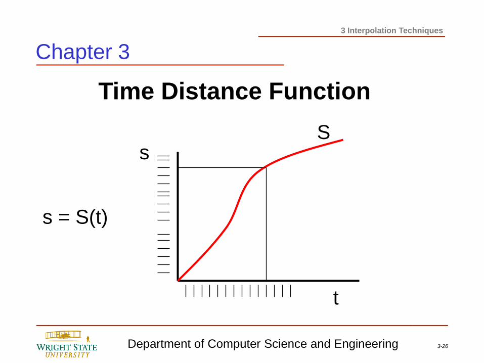
Time Distance Function
s = S(t)
s
t
S
Chapter 3
3-27 Department of Computer Science and Engineering
3 Interpolation Techniques
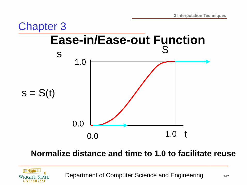
Ease-in/Ease-out Function
s = S(t)
s
t
S
0.0
0.0
1.0
1.0
Normalize distance and time to 1.0 to facilitate reuse
Chapter 3
3-28 Department of Computer Science and Engineering
3 Interpolation Techniques
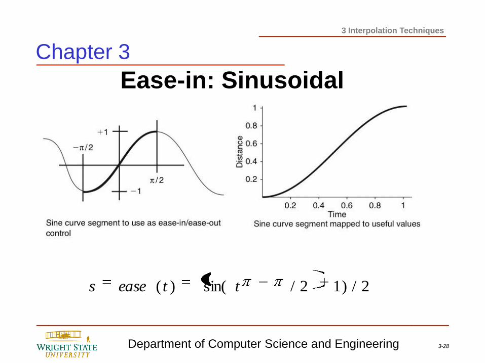
Ease-in: Sinusoidal
2/)12/sin()( tteases
Chapter 3
3-29 Department of Computer Science and Engineering
3 Interpolation Techniques
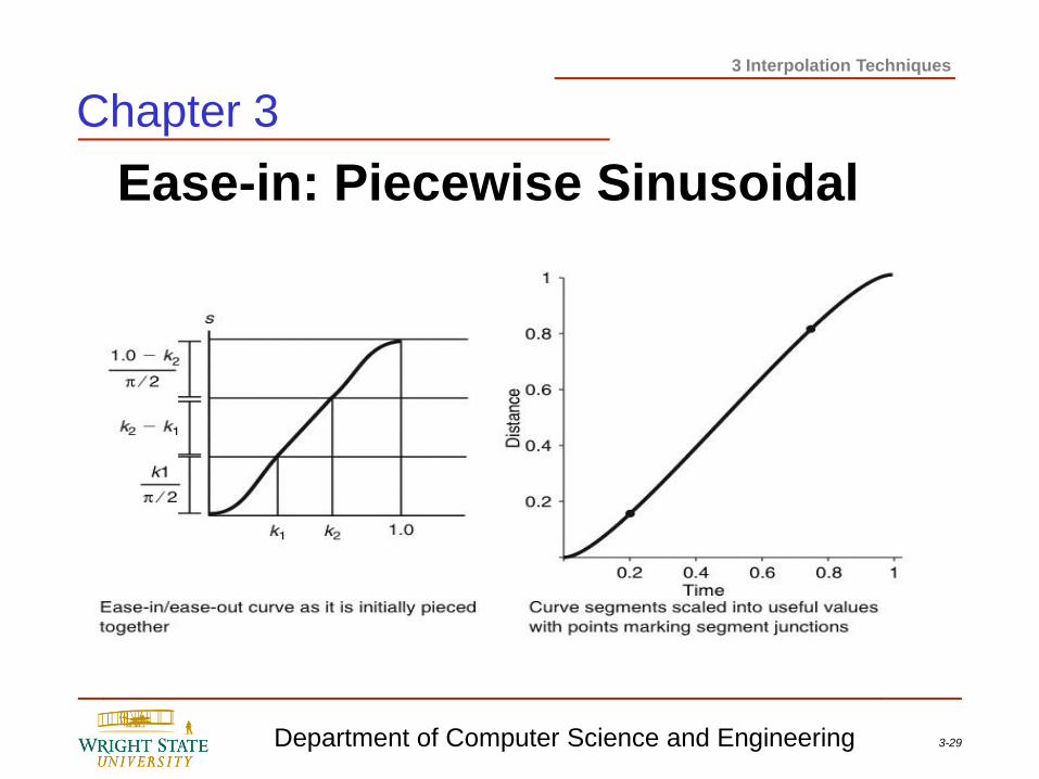
Ease-in: Piecewise Sinusoidal
Chapter 3
3-30 Department of Computer Science and Engineering
3 Interpolation Techniques
Ease-in: Piecewise Sinusoidal
)( tease
fk
tk /))
22(sin(
2(
1
1
fktk
/)2/
(1
1
fk
ktkkk
k/))
)1(2
)(sin(
2)1(
2/(
2
2
212
1
1kt
21ktk
tk2
Provides linear (constant velocity) middle segment
Chapter 3
3-31 Department of Computer Science and Engineering
3 Interpolation Techniques
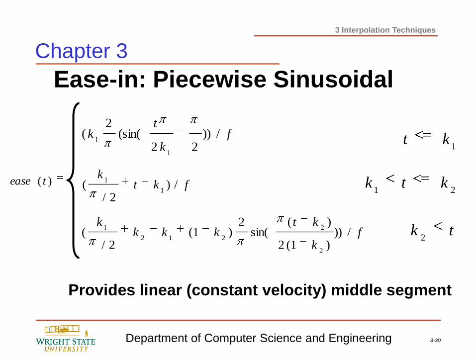
Ease-in: Single Cubic
2332)( ttteases
Chapter 3
Drawback: no segment of constant speed
3-32 Department of Computer Science and Engineering
3 Interpolation Techniques
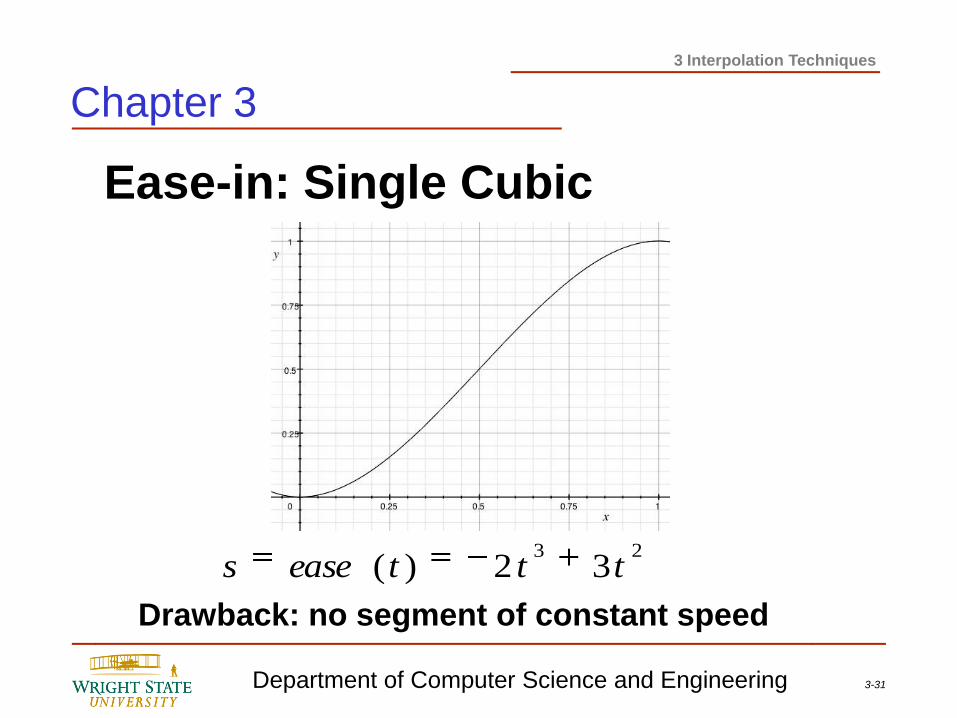
Ease-in: Constant Acceleration
Chapter 3
3-33 Department of Computer Science and Engineering
3 Interpolation Techniques
Ease-in: Constant Acceleration
Chapter 3
3-34 Department of Computer Science and Engineering
3 Interpolation Techniques
Ease-in: Constant Acceleration
Chapter 3
3-35 Department of Computer Science and Engineering
3 Interpolation Techniques
Ease-in: Constant Acceleration
Chapter 3
Integration of acceleration gives us desired function:
3-36 Department of Computer Science and Engineering
3 Interpolation Techniques
Arbitrary Speed Control
Animators can work in:
Distance-time space curves
Velocity-time space curves
Acceleration-time space curves
Set time-distance constraints
etc.
Chapter 3
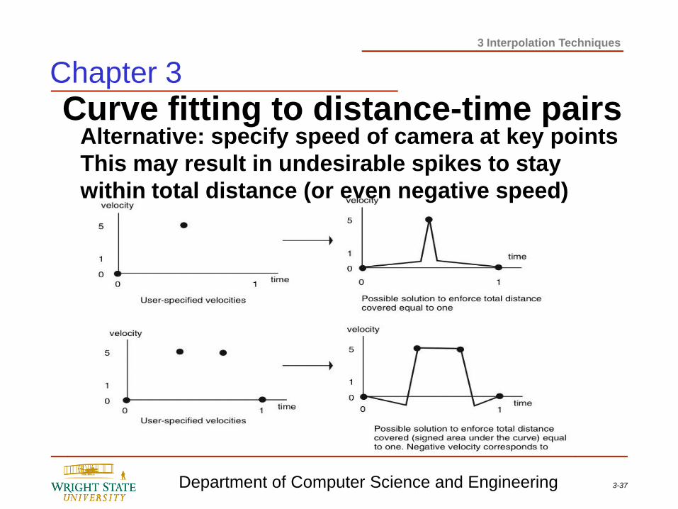
3-37 Department of Computer Science and Engineering
3 Interpolation Techniques
Curve fitting to distance-time pairs Chapter 3
Alternative: specify speed of camera at key points
This may result in undesirable spikes to stay
within total distance (or even negative speed)
3-38 Department of Computer Science and Engineering
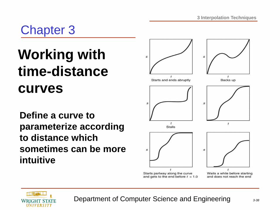
3 Interpolation Techniques
Working with
time-distance
curves
Chapter 3
Define a curve to
parameterize according
to distance which
sometimes can be more
intuitive
3-39 Department of Computer Science and Engineering
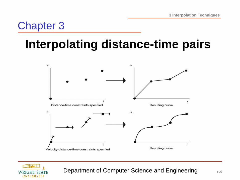
3 Interpolation Techniques
Interpolating distance-time pairs
Chapter 3
3-40 Department of Computer Science and Engineering
3 Interpolation Techniques
Chapter 3
Now that we have the camera path defined:
Is this all we need?
Looking at the function gluLookAt already tells us that we
need more information in form of the up vector and the
view direction or center point
3-41 Department of Computer Science and Engineering
3 Interpolation Techniques
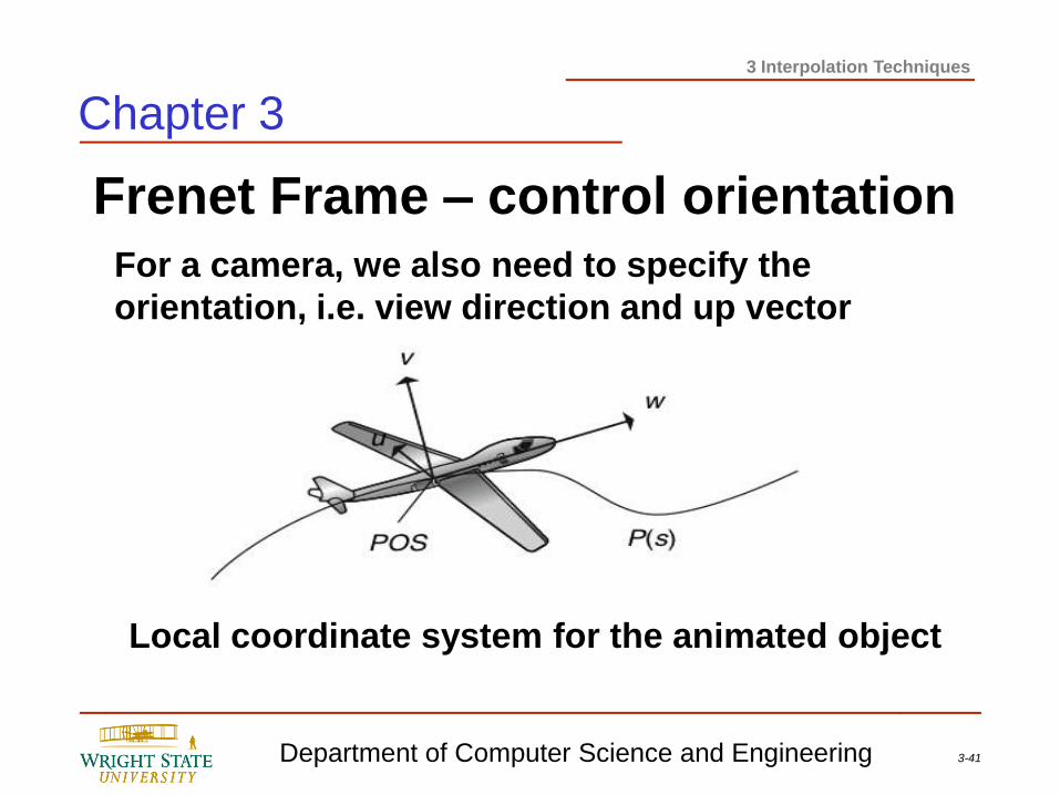
Frenet Frame – control orientation
Chapter 3
Local coordinate system for the animated object
For a camera, we also need to specify the
orientation, i.e. view direction and up vector
3-42 Department of Computer Science and Engineering
3 Interpolation Techniques
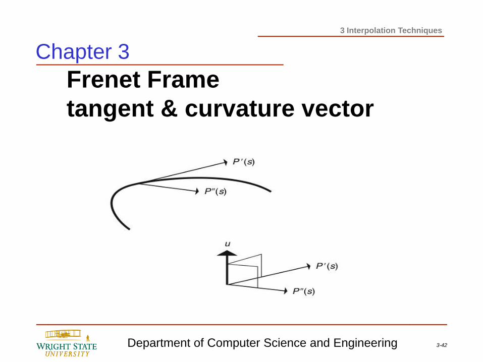
Frenet Frame
tangent & curvature vector
Chapter 3
3-43 Department of Computer Science and Engineering
3 Interpolation Techniques
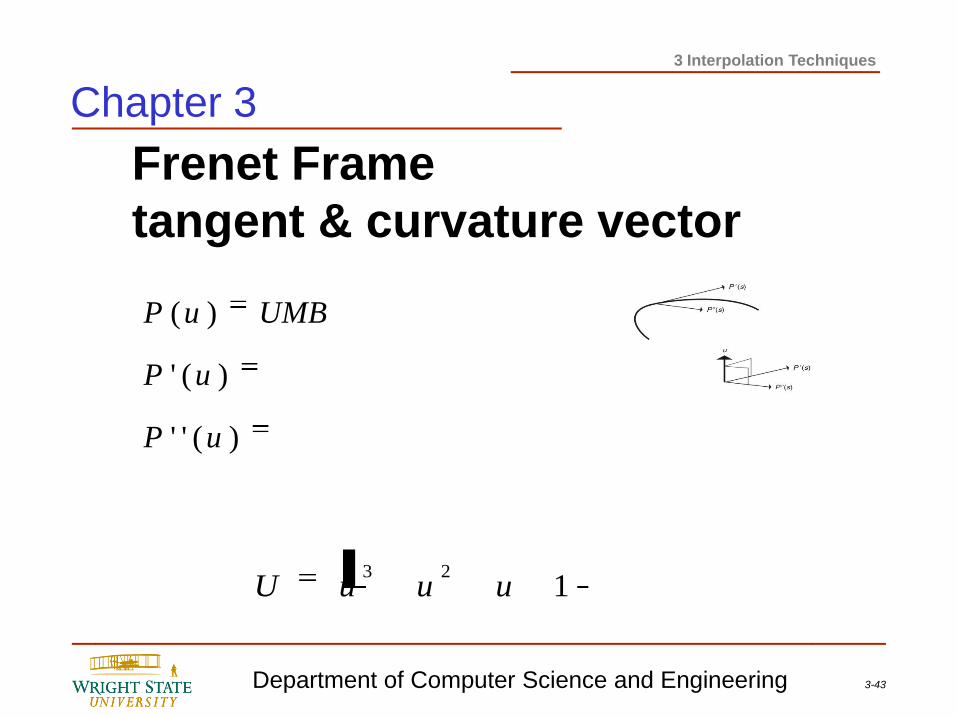
Frenet Frame
tangent & curvature vector
)(''
)('
)(
uP
uP
UMBuP
123
uuuU
Chapter 3
3-44 Department of Computer Science and Engineering
3 Interpolation Techniques
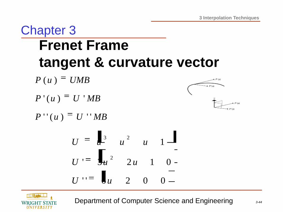
Frenet Frame
tangent & curvature vector
MBUuP
MBUuP
UMBuP
'')(''
')('
)(
0026''
0123'
1
2
23
uU
uuU
uuuU
Chapter 3
3-45 Department of Computer Science and Engineering
3 Interpolation Techniques
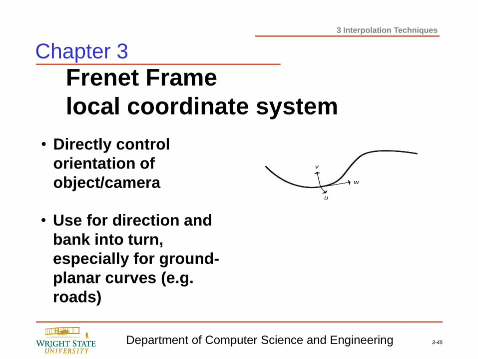
Frenet Frame
local coordinate system
• Directly control
orientation of
object/camera
• Use for direction and
bank into turn,
especially for ground-
planar curves (e.g.
roads)
Chapter 3
3-46 Department of Computer Science and Engineering
3 Interpolation Techniques
Frenet Frame - undefined
Chapter 3
Solution: interpolate between known vectors
3-47 Department of Computer Science and Engineering
3 Interpolation Techniques
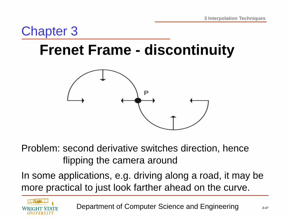
Frenet Frame - discontinuity
Chapter 3
Problem: second derivative switches direction, hence
flipping the camera around
In some applications, e.g. driving along a road, it may be
more practical to just look farther ahead on the curve.
3-48 Department of Computer Science and Engineering
3 Interpolation Techniques
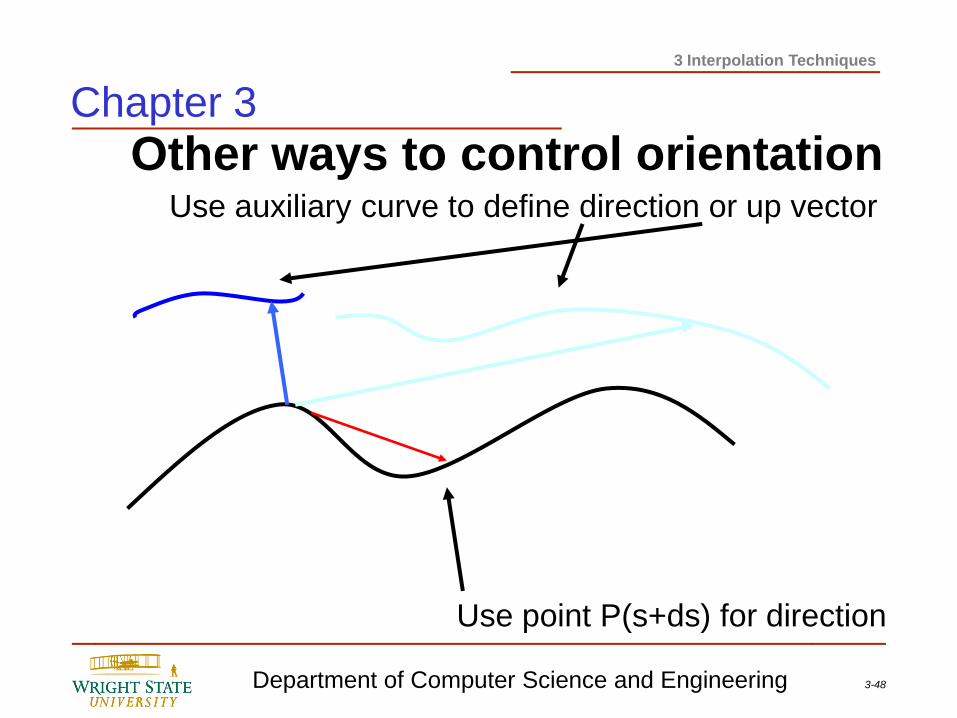
Other ways to control orientation
Use point P(s+ds) for direction
Use auxiliary curve to define direction or up vector
Chapter 3
3-49 Department of Computer Science and Engineering
3 Interpolation Techniques
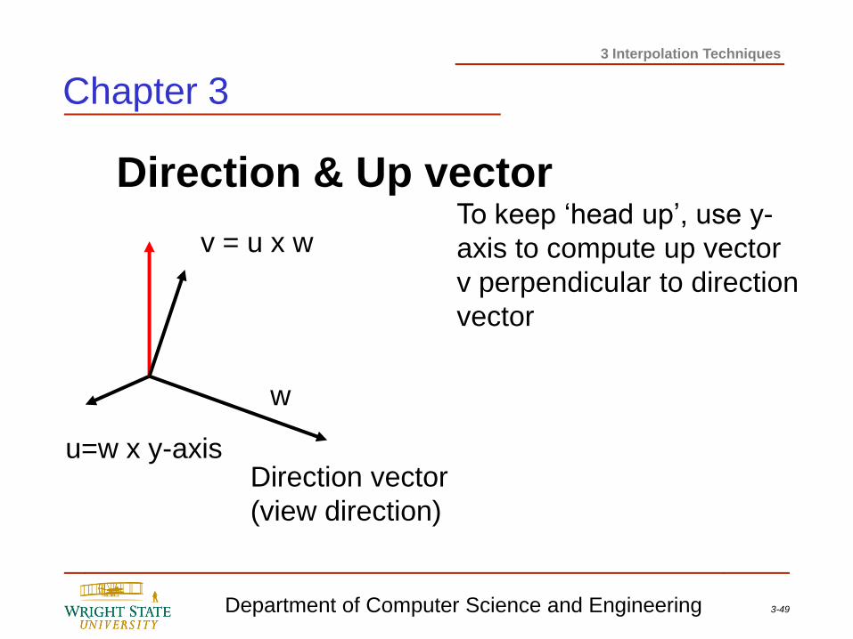
Direction & Up vector
Direction vector
(view direction)
w
u=w x y-axis
v = u x w To keep ‘head up’, use y-
axis to compute up vector
v perpendicular to direction
vector
Chapter 3
3-50 Department of Computer Science and Engineering
3 Interpolation Techniques
Chapter 3
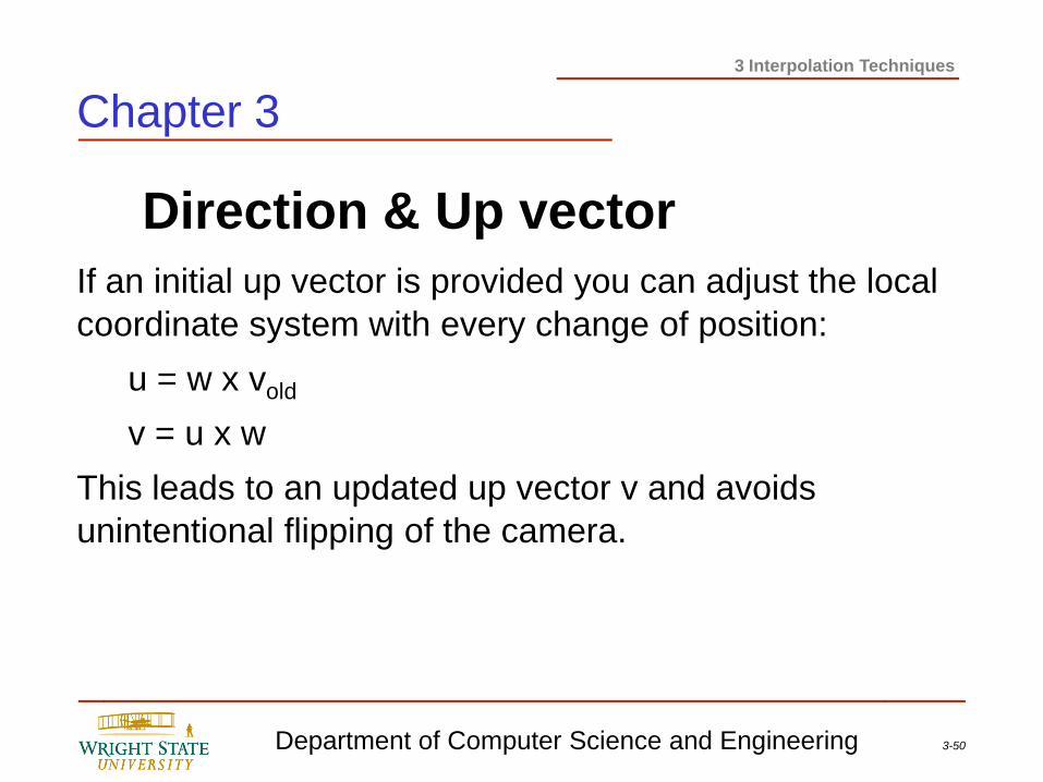
If an initial up vector is provided you can adjust the local
coordinate system with every change of position:
u = w x vold
v = u x w
This leads to an updated up vector v and avoids
unintentional flipping of the camera.
Direction & Up vector
3-51 Department of Computer Science and Engineering
3 Interpolation Techniques
Orientation interpolation
Preliminary note:
1. Remember that
2. Affects of scale are divided out by the inverse
appearing in quaternion rotation
3. When interpolating quaternions, use UNIT
quaternions – otherwise magnitudes can
interfere with spacing of results of interpolation
4. Unit quaternions can be interpreted as points on
a 4-D unit sphere
)()( vRotvRotkqq
Chapter 3
3-52 Department of Computer Science and Engineering
3 Interpolation Techniques
Orientation interpolation
2 problems analogous to issues when interpolating
positions: 1. How to take equi-distant steps along orientation
path?
2. How to pass through orientations smoothly (1st
order continuous)
3. And another particular to quaternions: with dual
unit quaternion representations, which to use?
Quaternions can be interpolated to produce in-
between orientations:
21)1( kqqkq
Chapter 3
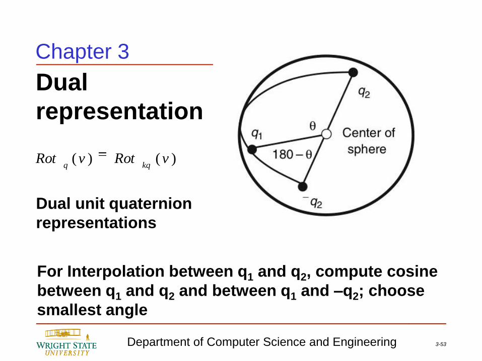
3-53 Department of Computer Science and Engineering
3 Interpolation Techniques
Dual
representation
Dual unit quaternion
representations
)()( vRotvRotkqq
For Interpolation between q1 and q2, compute cosine
between q1 and q2 and between q1 and –q2; choose
smallest angle
Chapter 3
3-54 Department of Computer Science and Engineering
3 Interpolation Techniques
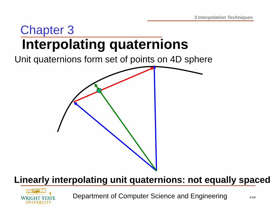
Interpolating quaternions
Linearly interpolating unit quaternions: not equally spaced
Unit quaternions form set of points on 4D sphere
Chapter 3
3-55 Department of Computer Science and Engineering
3 Interpolation Techniques
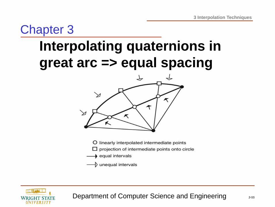
Interpolating quaternions in
great arc => equal spacing
Chapter 3
3-56 Department of Computer Science and Engineering
3 Interpolation Techniques
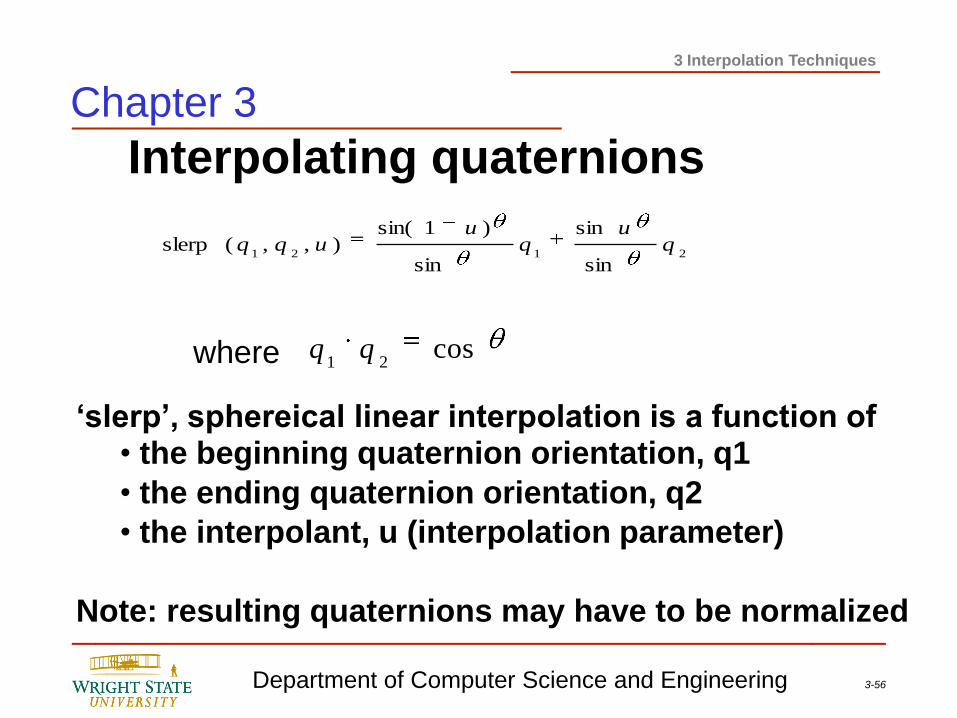
Interpolating quaternions
2121
sin
sin
sin
)1sin(),,(slerp q
uq
uuqq
‘slerp’, sphereical linear interpolation is a function of • the beginning quaternion orientation, q1
• the ending quaternion orientation, q2
• the interpolant, u (interpolation parameter)
Note: resulting quaternions may have to be normalized
cos21
qqwhere
Chapter 3
3-57 Department of Computer Science and Engineering
3 Interpolation Techniques
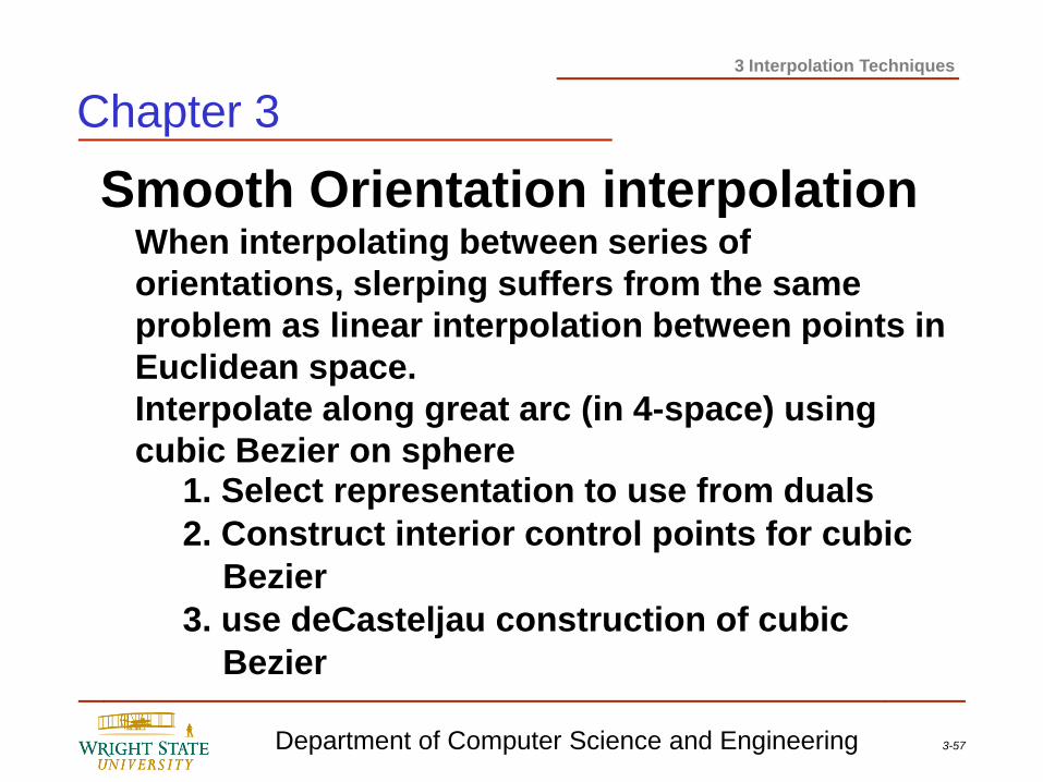
Smooth Orientation interpolation When interpolating between series of
orientations, slerping suffers from the same
problem as linear interpolation between points in
Euclidean space.
Interpolate along great arc (in 4-space) using
cubic Bezier on sphere 1. Select representation to use from duals
2. Construct interior control points for cubic
Bezier
3. use deCasteljau construction of cubic
Bezier
Chapter 3
3-58 Department of Computer Science and Engineering
3 Interpolation Techniques
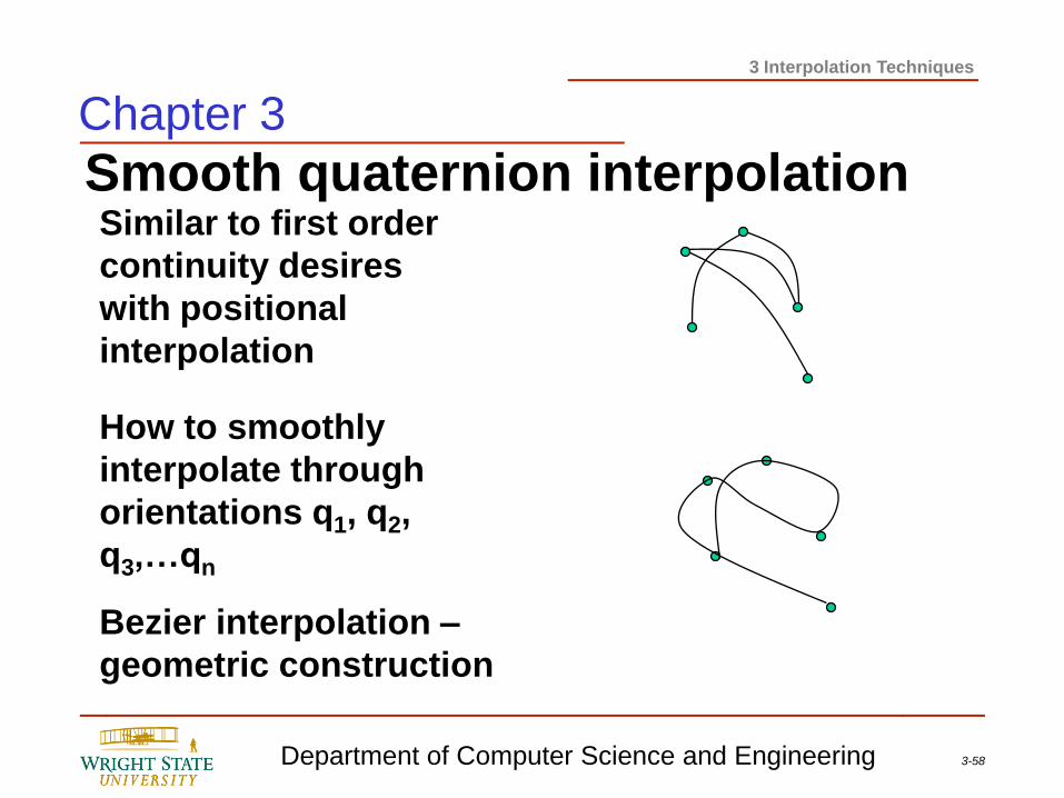
Smooth quaternion interpolation
How to smoothly
interpolate through
orientations q1, q2,
q3,…qn
Similar to first order
continuity desires
with positional
interpolation
Bezier interpolation –
geometric construction
Chapter 3
3-59 Department of Computer Science and Engineering
3 Interpolation Techniques
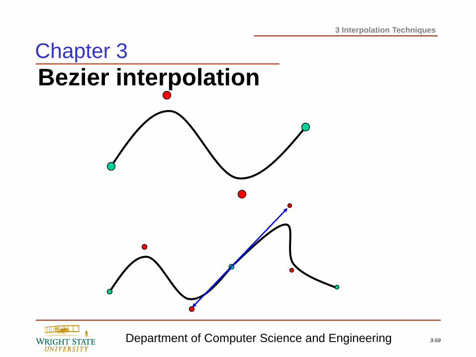
Bezier interpolation Chapter 3
3-60 Department of Computer Science and Engineering
3 Interpolation Techniques
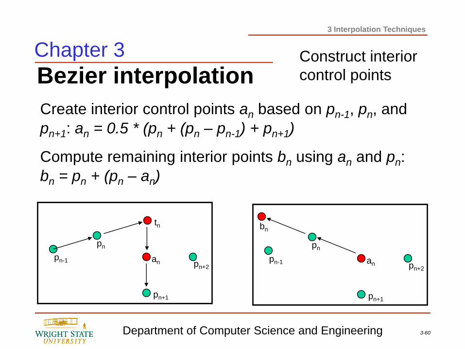
Bezier interpolation Construct interior
control points
pn-1
pn
pn+1
pn+2 an
tn
pn-1
pn
pn+1
pn+2 an
bn
Chapter 3
Create interior control points an based on pn-1, pn, and
pn+1: an = 0.5 * (pn + (pn – pn-1) + pn+1)
Compute remaining interior points bn using an and pn:
bn = pn + (pn – an)
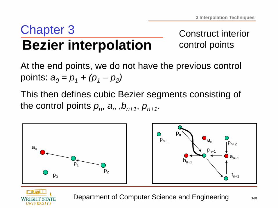
3-61 Department of Computer Science and Engineering
3 Interpolation Techniques
Bezier interpolation Construct interior
control points
pn-1
pn
pn+1
pn+2 an
tn+1
an+1 bn+1
p2
p1
p0
a0
Chapter 3
At the end points, we do not have the previous control
points: a0 = p1 + (p1 – p2)
This then defines cubic Bezier segments consisting of
the control points pn, an ,bn+1, pn+1.
3-62 Department of Computer Science and Engineering
3 Interpolation Techniques
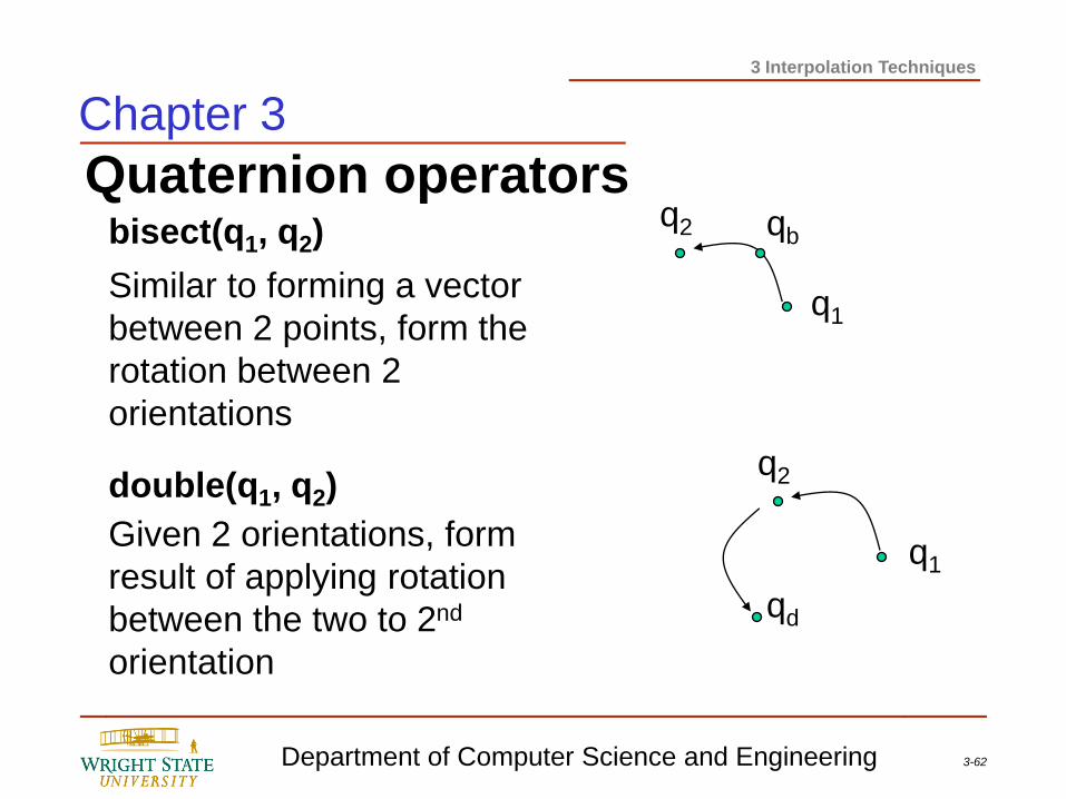
Quaternion operators
Similar to forming a vector
between 2 points, form the
rotation between 2
orientations
Given 2 orientations, form
result of applying rotation
between the two to 2nd
orientation
q1
q2
q1
q2
qd
double(q1, q2)
bisect(q1, q2) qb
Chapter 3
3-63 Department of Computer Science and Engineering
3 Interpolation Techniques
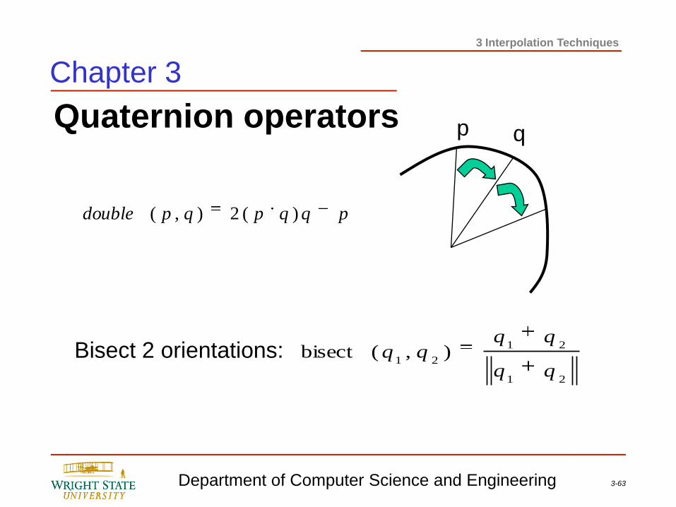
Quaternion operators
pqqpqpdouble )(2),(
Bisect 2 orientations: 21
21
21),(bisect
qqqq
p q
Chapter 3
3-64 Department of Computer Science and Engineering
3 Interpolation Techniques
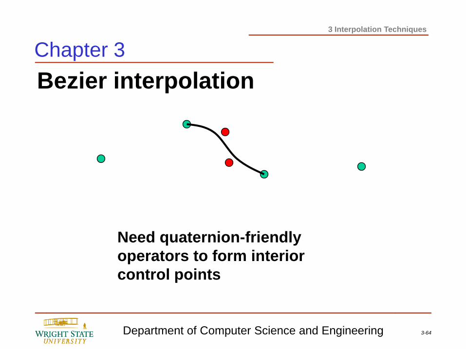
Bezier interpolation
Need quaternion-friendly
operators to form interior
control points
Chapter 3
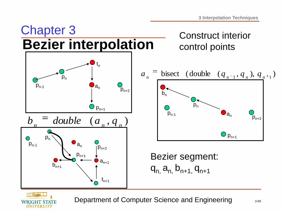
3-65 Department of Computer Science and Engineering
3 Interpolation Techniques
Bezier interpolation Construct interior
control points
)),,(double(bisect11 nnnn
qqqa
),(nnn
qadoubleb
Bezier segment:
qn, an, bn+1, qn+1
pn-1
pn
pn+1
pn+2 an
tn
pn-1
pn
pn+1
pn+2 an
bn
pn-1
pn
pn+1
pn+2 an
tn+1
an+1 bn+1
Chapter 3
3-66 Department of Computer Science and Engineering
3 Interpolation Techniques
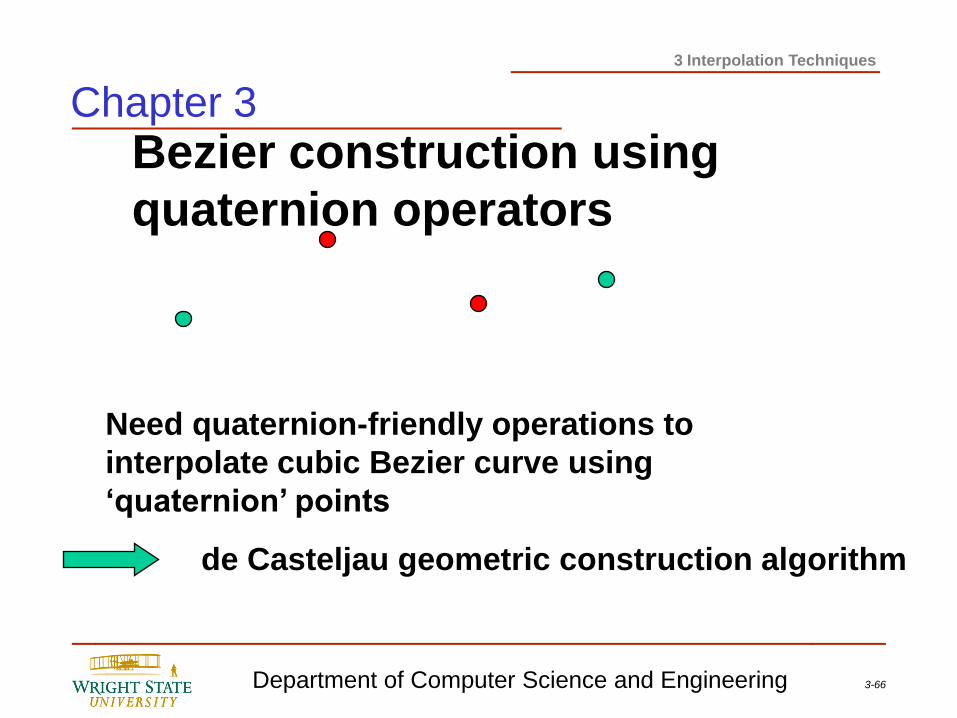
Bezier construction using
quaternion operators
Need quaternion-friendly operations to
interpolate cubic Bezier curve using
‘quaternion’ points
de Casteljau geometric construction algorithm
Chapter 3
3-67 Department of Computer Science and Engineering
3 Interpolation Techniques
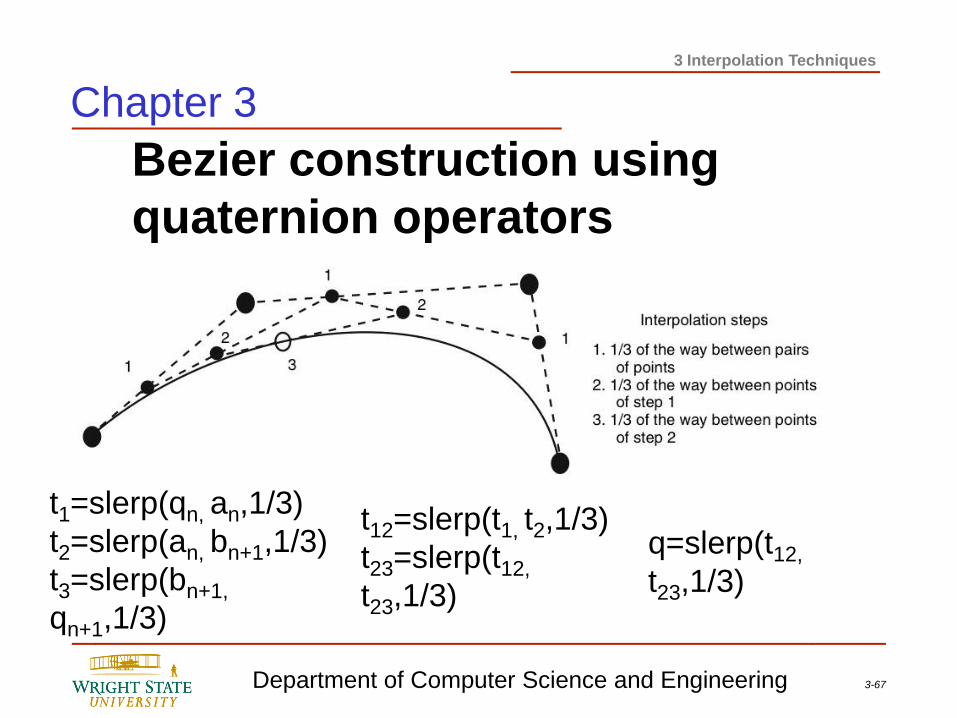
Bezier construction using
quaternion operators
t1=slerp(qn, an,1/3)
t2=slerp(an, bn+1,1/3)
t3=slerp(bn+1,
qn+1,1/3)
t12=slerp(t1, t2,1/3)
t23=slerp(t12,
t23,1/3)
q=slerp(t12,
t23,1/3)
Chapter 3
3-68 Department of Computer Science and Engineering
3 Interpolation Techniques
Working with paths
For cases in which the points making up a path are
generated by a digitizing process, the resulting curve
can be too jerky because of noise or imprecision. To
remove the jerkiness, the coordinate values of the
data can be smoothed by one of several approaches:
Smoothing a path
Determining a path along a surface
Finding downhill direction
Chapter 3
3-69 Department of Computer Science and Engineering
3 Interpolation Techniques
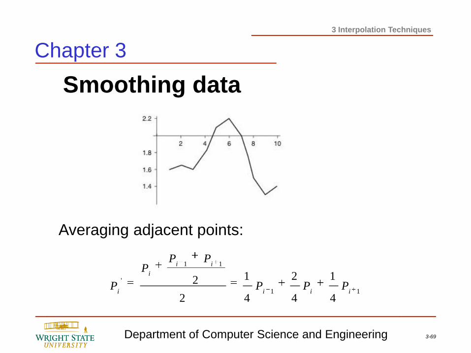
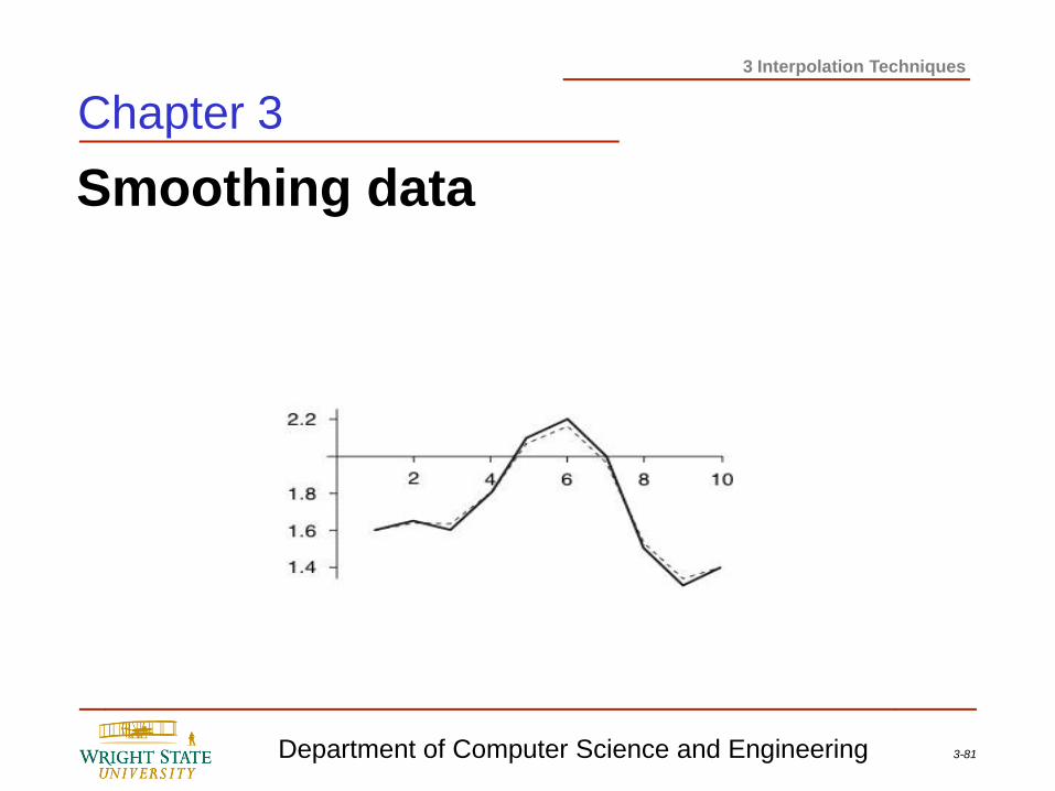
Smoothing data
Chapter 3
Averaging adjacent points:
11
11
'
4
1
4
2
4
1
2
2iii
ii
i
iPPP
PPP
P
3-70 Department of Computer Science and Engineering
3 Interpolation Techniques
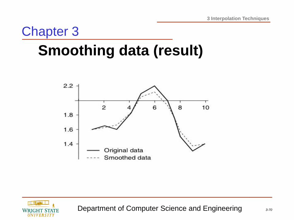
Smoothing data (result)
Chapter 3
3-71 Department of Computer Science and Engineering
3 Interpolation Techniques
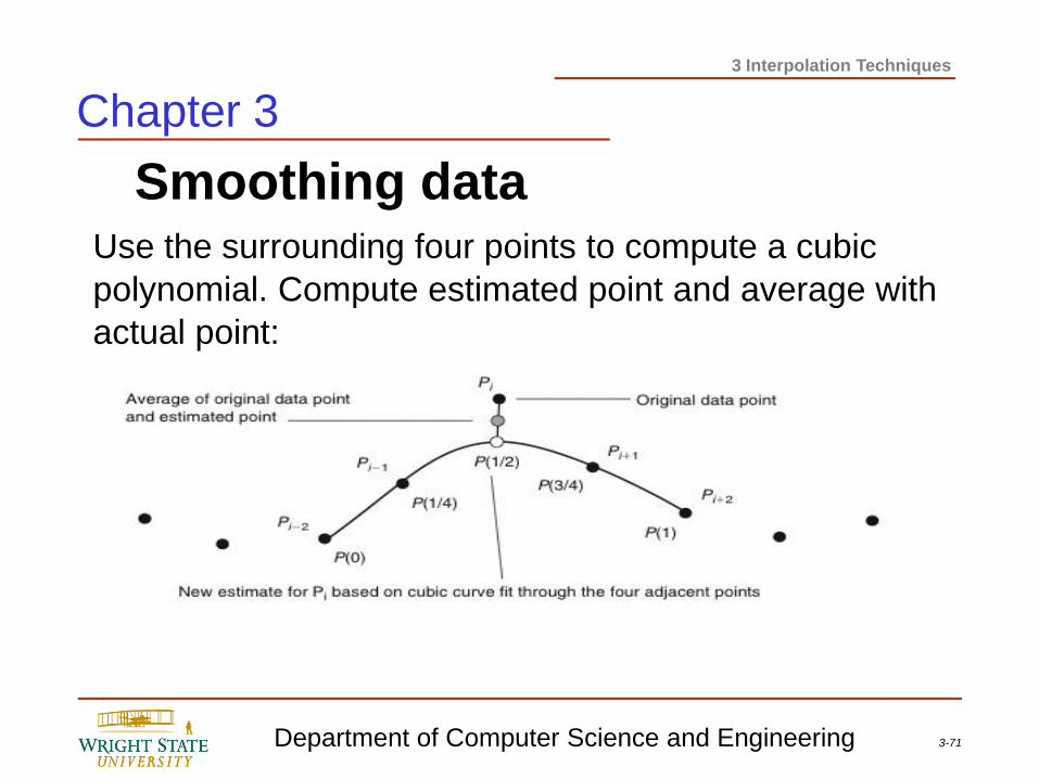
Smoothing data
Chapter 3
Use the surrounding four points to compute a cubic
polynomial. Compute estimated point and average with
actual point:
3-72 Department of Computer Science and Engineering
3 Interpolation Techniques
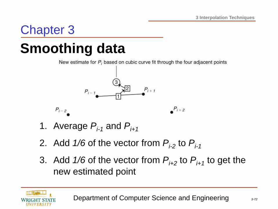
Smoothing data
Chapter 3
1. Average Pi-1 and Pi+1
2. Add 1/6 of the vector from Pi-2 to Pi-1
3. Add 1/6 of the vector from Pi+2 to Pi+1 to get the
new estimated point
3-73 Department of Computer Science and Engineering
3 Interpolation Techniques
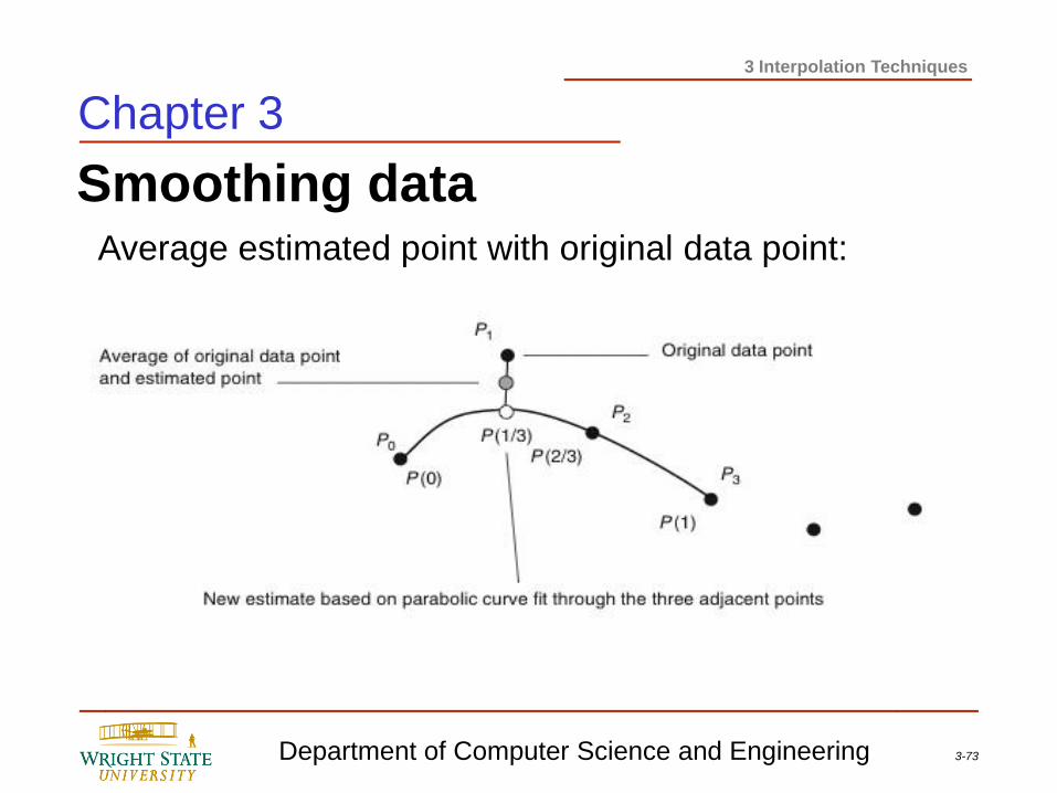
Smoothing data
Chapter 3
Average estimated point with original data point:
3-74 Department of Computer Science and Engineering
3 Interpolation Techniques
Smoothing data
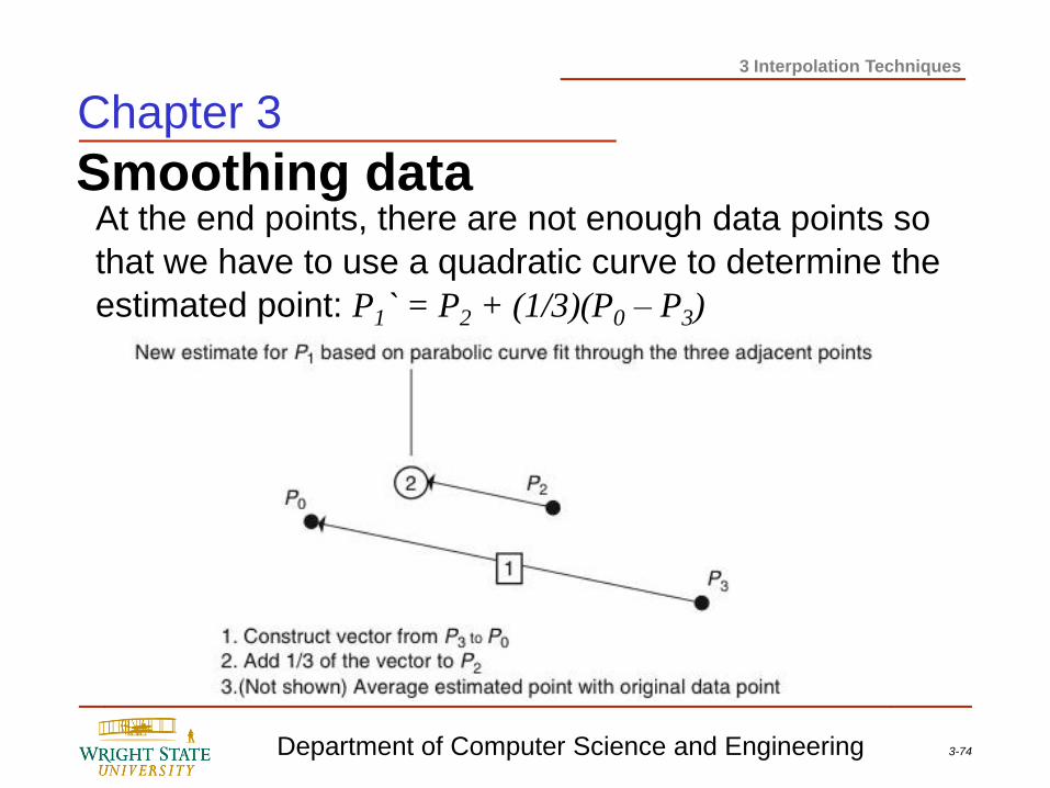
Chapter 3
At the end points, there are not enough data points so
that we have to use a quadratic curve to determine the
estimated point: P1` = P2 + (1/3)(P0 – P3)
3-75 Department of Computer Science and Engineering
3 Interpolation Techniques
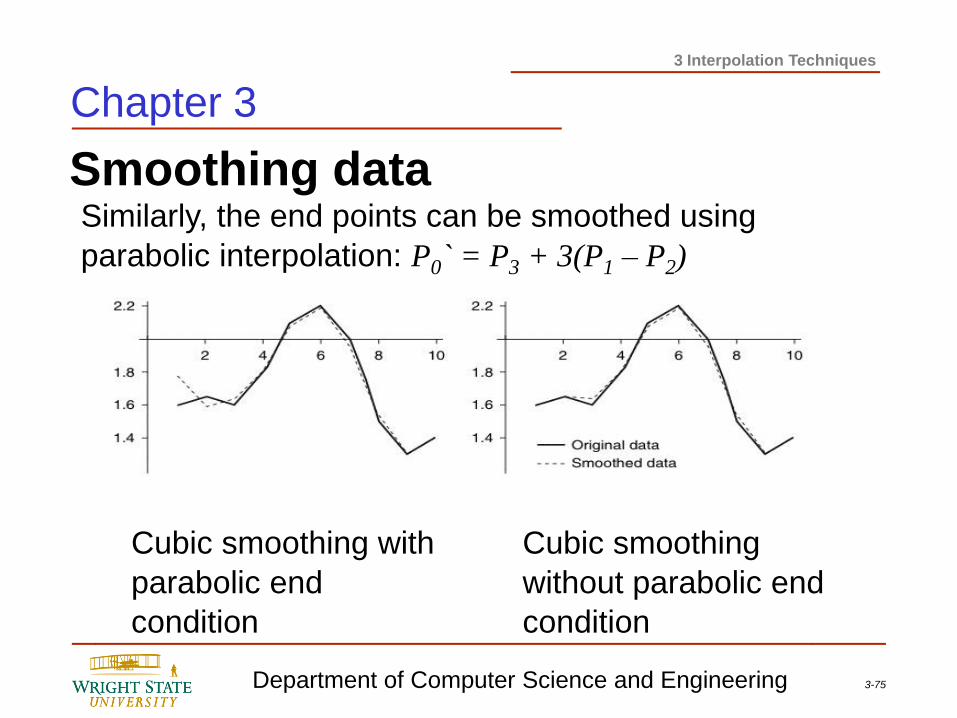
Smoothing data
Chapter 3
Cubic smoothing with
parabolic end
condition
Cubic smoothing
without parabolic end
condition
Similarly, the end points can be smoothed using
parabolic interpolation: P0` = P3 + 3(P1 – P2)
3-76 Department of Computer Science and Engineering
3 Interpolation Techniques
Smoothing data
Chapter 3
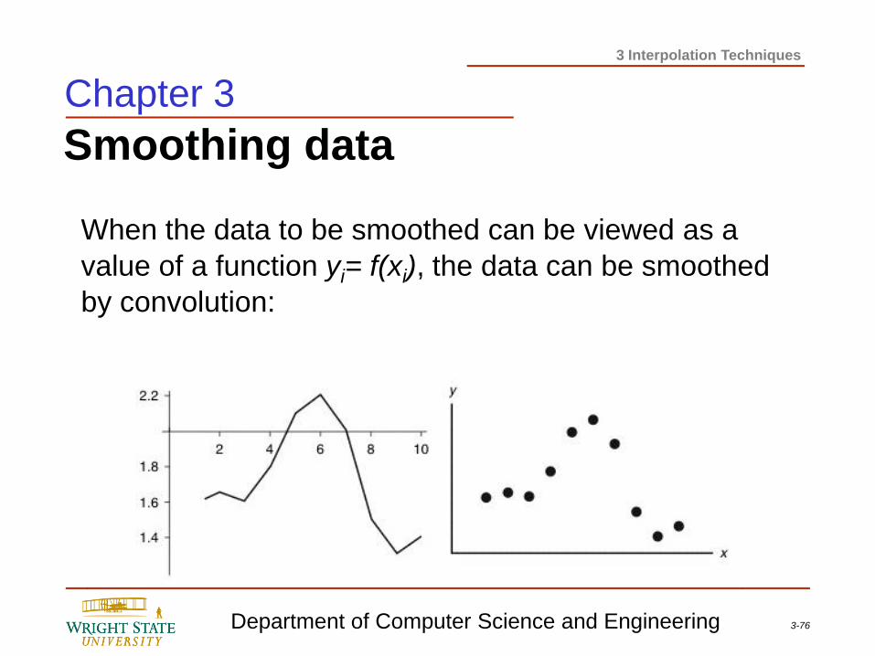
When the data to be smoothed can be viewed as a
value of a function yi= f(xi), the data can be smoothed
by convolution:
3-77 Department of Computer Science and Engineering
3 Interpolation Techniques
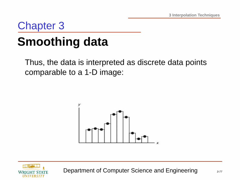
Smoothing data
Chapter 3
Thus, the data is interpreted as discrete data points
comparable to a 1-D image:
3-78 Department of Computer Science and Engineering
3 Interpolation Techniques
Chapter 3
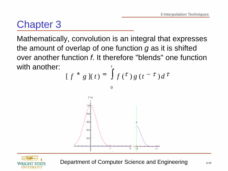
Mathematically, convolution is an integral that expresses
the amount of overlap of one function g as it is shifted
over another function f. It therefore "blends" one function
with another: t
dtgftgf
0
)()()]([
3-79 Department of Computer Science and Engineering
3 Interpolation Techniques
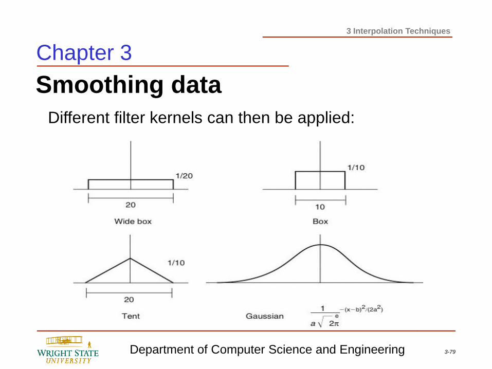
Smoothing data
Chapter 3
Different filter kernels can then be applied:
3-80 Department of Computer Science and Engineering
3 Interpolation Techniques
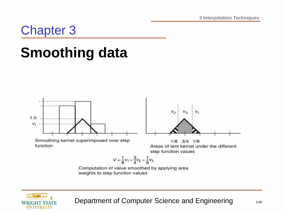
Smoothing data
Chapter 3
3-81 Department of Computer Science and Engineering
3 Interpolation Techniques
Smoothing data
Chapter 3
3-82 Department of Computer Science and Engineering
3 Interpolation Techniques
Chapter 3
Path finding
If one object is to move across the surface of another
object, then a path across the surface must be
determined. If start and destination points are known, it
can be computationally expensive to find the shortest
path between the points. However, it is not often
necessary to find the absolute shortest path. Various
alternatives exist for determining suboptimal, yet more-or-
less direct paths.
3-83 Department of Computer Science and Engineering
3 Interpolation Techniques
Chapter 3
Path finding
An easy way to determine a path along a polygonal
surface mesh is to determine a plane that contains the
two points and is generally perpendicular to the surface.
Generally perpendicular can be defined, for example, as
the average of the two vertex normals that the path is
being formed between. The intersection of the plane with
the faces making up the surface mesh will define a path
between the two points.
3-84 Department of Computer Science and Engineering
3 Interpolation Techniques
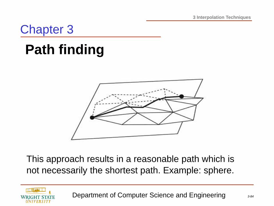
Path finding
Chapter 3
This approach results in a reasonable path which is
not necessarily the shortest path. Example: sphere.
3-85 Department of Computer Science and Engineering
3 Interpolation Techniques
Chapter 3
Path finding – downhill
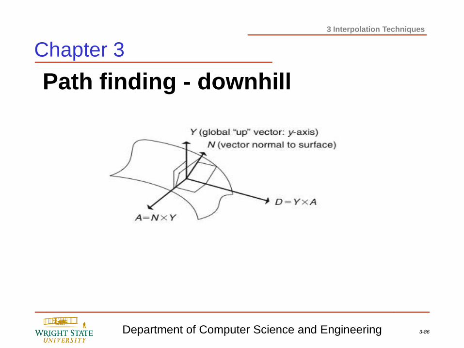
If a path downhill from an initial point on the surface is
desired, then the surface normal and global up vector can
be used to determine the downhill vector. The cross
product of the normal and global up vector defines a
vector that lies on the surface perpendicular to the
downhill direction. So the cross product of this vector and
the normal vector defines the downhill (and uphill) vector
on a plane. This same approach works with curved
surfaces to produce the instantaneous downhill vector.
3-86 Department of Computer Science and Engineering
3 Interpolation Techniques
Path finding - downhill
Chapter 3
3-87 Department of Computer Science and Engineering
3 Interpolation Techniques
Chapter 3
Interpolation-Based Animation
The techniques described so far describe the basics of
interpolating values. The remainder of this chapter
addresses how to use those basics to facilitate the
production of computer animation. Procedures and
algorithms are used in which the animator has very
specific expectations about the motion that will be
produced on a frame-by-frame basis.
3-88 Department of Computer Science and Engineering
3 Interpolation Techniques
Interpolation based animation
Key-frame systems – in general
Interpolating shapes Deforming a single shape
3D interpolation between two shapes
Morphing – deforming an image
Chapter 3
3-89 Department of Computer Science and Engineering
3 Interpolation Techniques
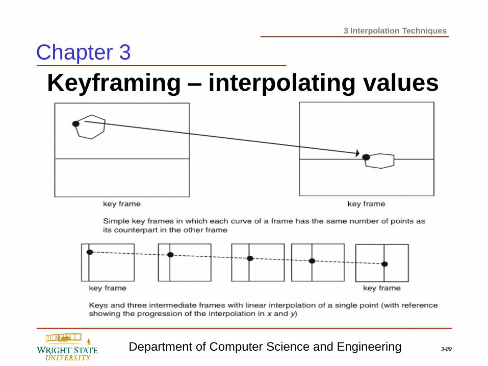
Keyframing – interpolating values
Chapter 3
3-90 Department of Computer Science and Engineering
3 Interpolation Techniques
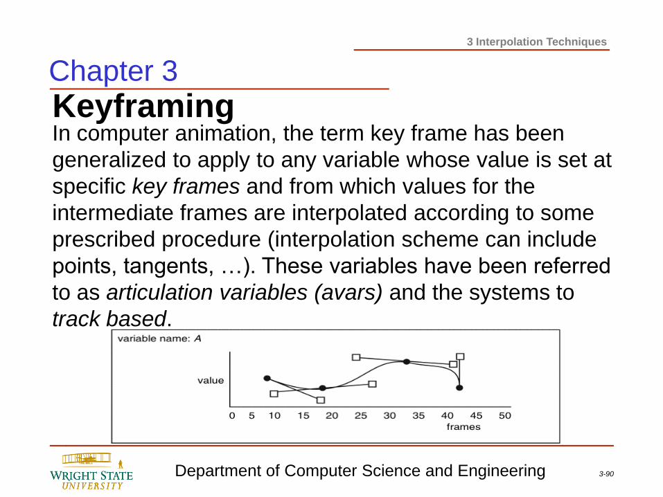
Keyframing In computer animation, the term key frame has been
generalized to apply to any variable whose value is set at
specific key frames and from which values for the
intermediate frames are interpolated according to some
prescribed procedure (interpolation scheme can include
points, tangents, …). These variables have been referred
to as articulation variables (avars) and the systems to
track based.
Chapter 3
3-91 Department of Computer Science and Engineering
3 Interpolation Techniques
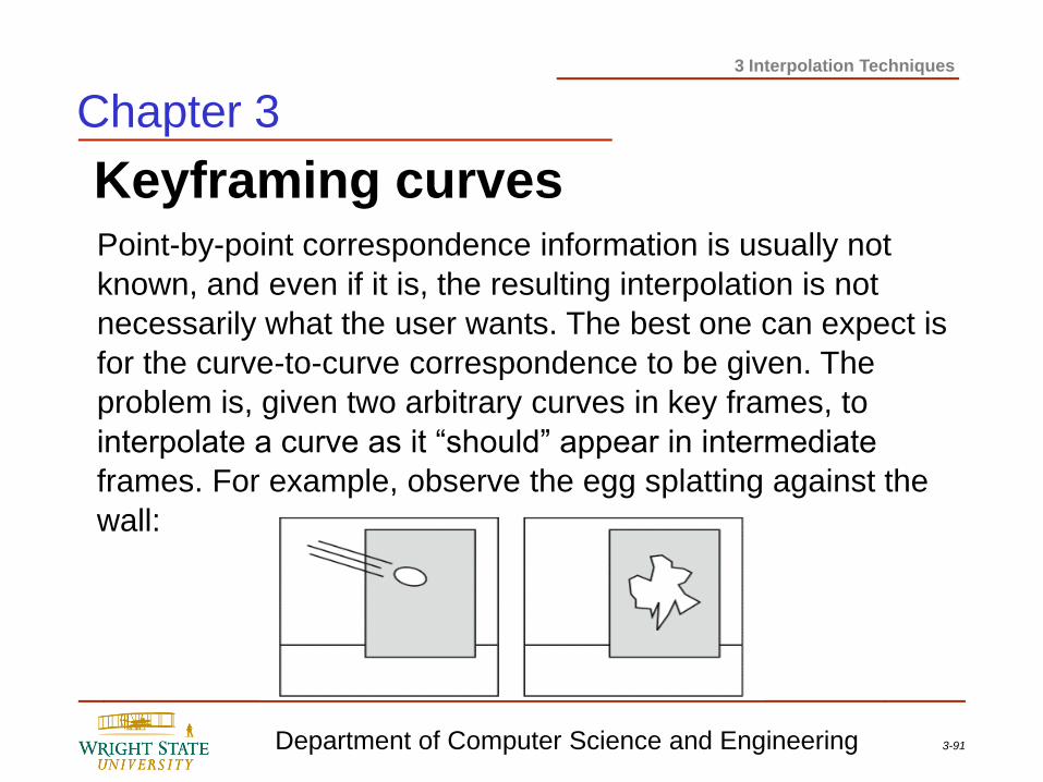
Keyframing curves
Chapter 3
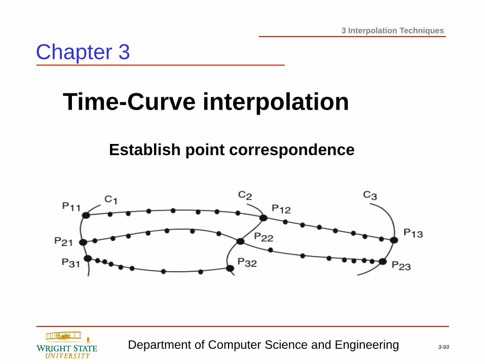
Point-by-point correspondence information is usually not
known, and even if it is, the resulting interpolation is not
necessarily what the user wants. The best one can expect is
for the curve-to-curve correspondence to be given. The
problem is, given two arbitrary curves in key frames, to
interpolate a curve as it “should” appear in intermediate
frames. For example, observe the egg splatting against the
wall:
3-92 Department of Computer Science and Engineering
3 Interpolation Techniques
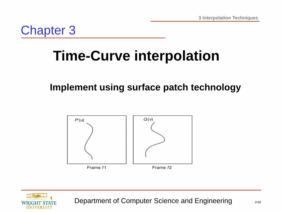
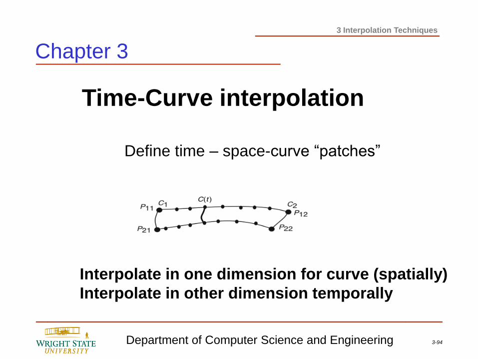
Time-Curve interpolation
Implement using surface patch technology
Chapter 3
3-93 Department of Computer Science and Engineering
3 Interpolation Techniques
Time-Curve interpolation
Establish point correspondence
Chapter 3
3-94 Department of Computer Science and Engineering
3 Interpolation Techniques
Time-Curve interpolation
Define time – space-curve “patches”
Interpolate in one dimension for curve (spatially)
Interpolate in other dimension temporally
Chapter 3
3-95 Department of Computer Science and Engineering
3 Interpolation Techniques
Object interpolation
1. Modify shape of object interpolate
vertices of different shapes
Correspondence problem
Interpolation problem
2. Interpolate one object into second
object
3. Interpolate one image into second
image
Chapter 3
3-96 Department of Computer Science and Engineering
3 Interpolation Techniques
Chapter 3
Deforming Objects
Deforming an object shape and transforming one shape
into another is a visually powerful animation technique. It
adds the notion of malleability and density. Flexible body
animation makes the objects in an animation seem much
more expressive and alive. There are physically based
approaches that simulate the reaction of objects
undergoing forces. However, many animators want more
precise control over the shape on an object than that
provided by simulations and/or do not want the
computational expense of the simulating physical
process.
3-97 Department of Computer Science and Engineering
3 Interpolation Techniques
Chapter 3
Deforming Objects
Instead, the animator may want to deform the object
directly and define key shapes. Shape definitions that
share the same edge connectivity can be interpolated on
a vertex-to-vertex basis in order to smoothly change from
one shape to the other. A sequence of key shapes can be
interpolated over time to produce flexible body animation.
Multivariate interpolation can be used to blend among a
number of different shapes. The various shapes are
referred to as blend shapes or morph targets and is a
commonly used technique in facial animation.
3-98 Department of Computer Science and Engineering
3 Interpolation Techniques
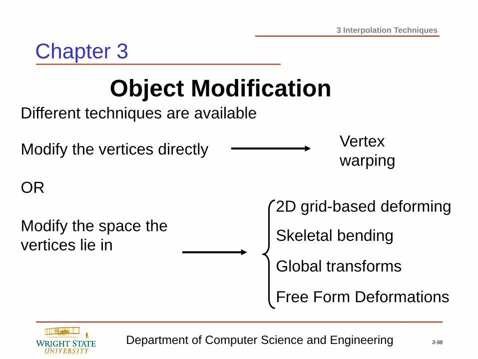
Object Modification
Vertex
warping
2D grid-based deforming
Skeletal bending
Free Form Deformations
Modify the vertices directly
OR
Modify the space the
vertices lie in
Global transforms
Chapter 3
Different techniques are available
3-99 Department of Computer Science and Engineering
3 Interpolation Techniques
Chapter 3
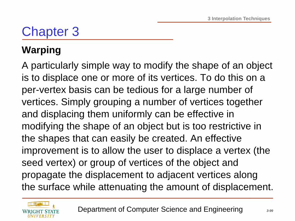
Warping
A particularly simple way to modify the shape of an object
is to displace one or more of its vertices. To do this on a
per-vertex basis can be tedious for a large number of
vertices. Simply grouping a number of vertices together
and displacing them uniformly can be effective in
modifying the shape of an object but is too restrictive in
the shapes that can easily be created. An effective
improvement is to allow the user to displace a vertex (the
seed vertex) or group of vertices of the object and
propagate the displacement to adjacent vertices along
the surface while attenuating the amount of displacement.
3-100 Department of Computer Science and Engineering
3 Interpolation Techniques
Warping
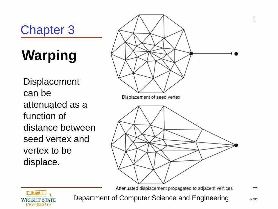
Chapter 3
Displacement
can be
attenuated as a
function of
distance between
seed vertex and
vertex to be
displace.
3-101 Department of Computer Science and Engineering
3 Interpolation Techniques
Chapter 3
Warping
Attenuation is typically a function of the distance metric.
The minimum of connecting edges is used for the
distance metric and the user specifies the maximum
range of effect to be vertices within n edges of the seed
vertex. A scale factor is applied to the displacement
vector according to the user-selected integer value of k as
shown on the next slide.
3-102 Department of Computer Science and Engineering
3 Interpolation Techniques
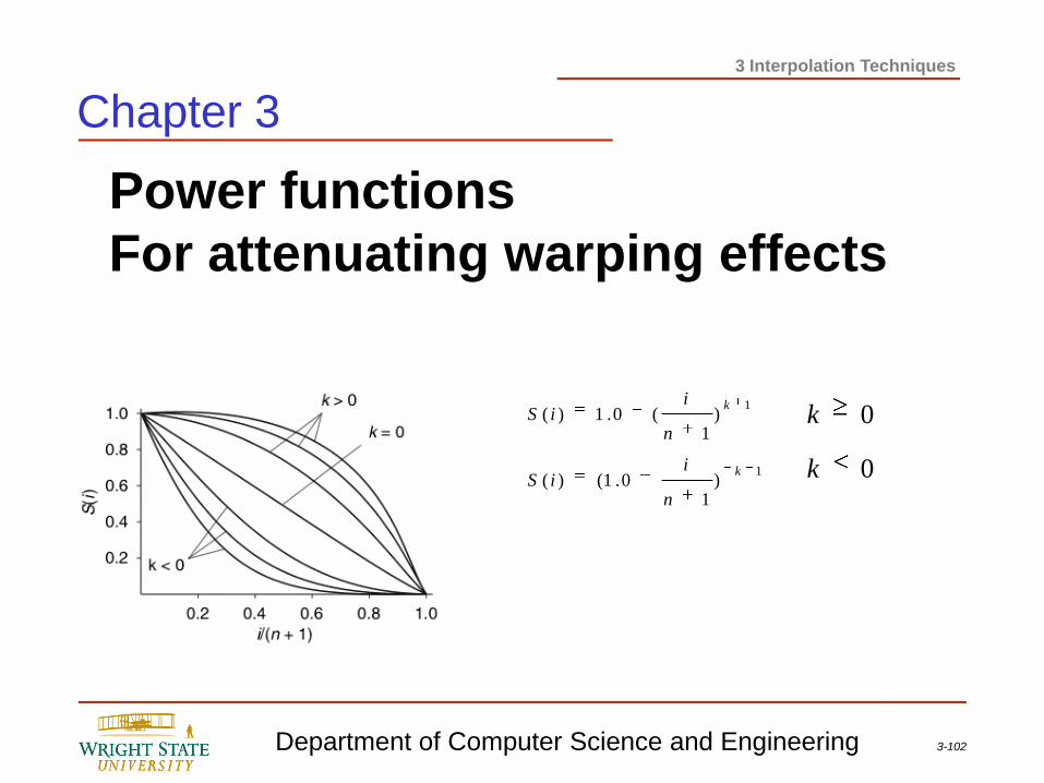
Power functions
For attenuating warping effects
1
1
)1
0.1()(
)1
(0.1)(
k
k
n
iiS
n
iiS
0
0
k
k
Chapter 3
3-103 Department of Computer Science and Engineering
3 Interpolation Techniques
Chapter 3
Warping
These attenuation functions are easy to compute and
provide sufficient flexibility for many desired effects.
When k equals zero it corresponds to a linear attenuation,
while values of k less than zero create a more elastic
impression. Values of k greater than zero create the
effect of more rigid displacements.
3-104 Department of Computer Science and Engineering
3 Interpolation Techniques
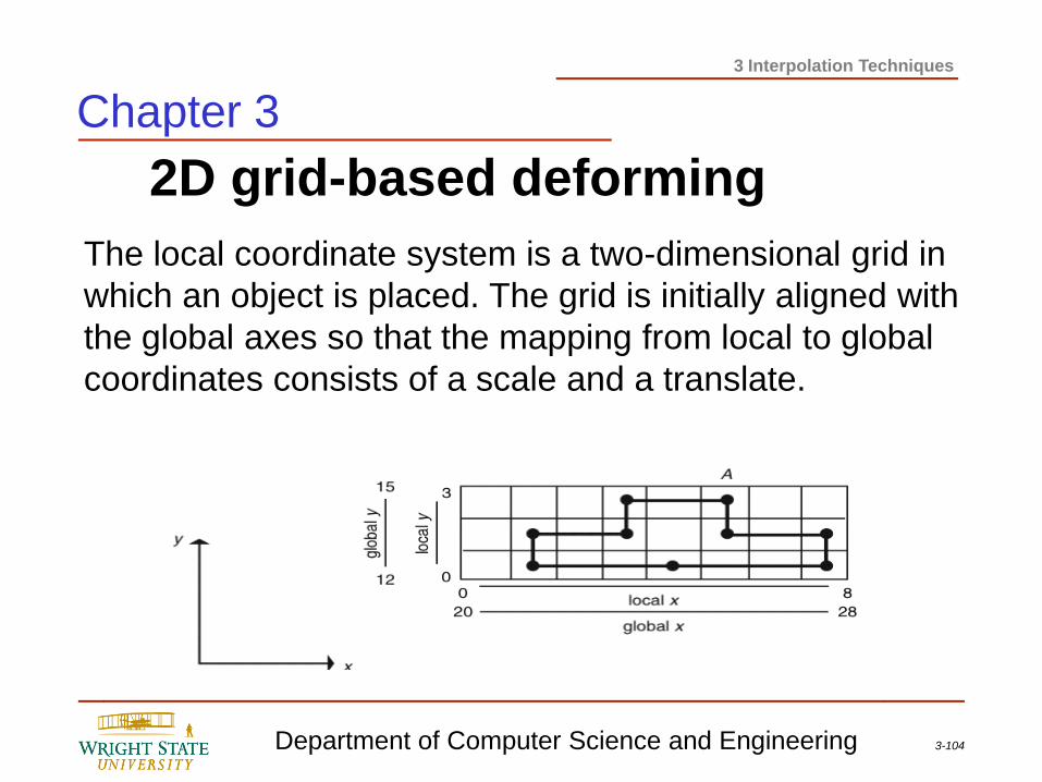
2D grid-based deforming
The local coordinate system is a two-dimensional grid in
which an object is placed. The grid is initially aligned with
the global axes so that the mapping from local to global
coordinates consists of a scale and a translate.
Chapter 3
3-105 Department of Computer Science and Engineering
3 Interpolation Techniques
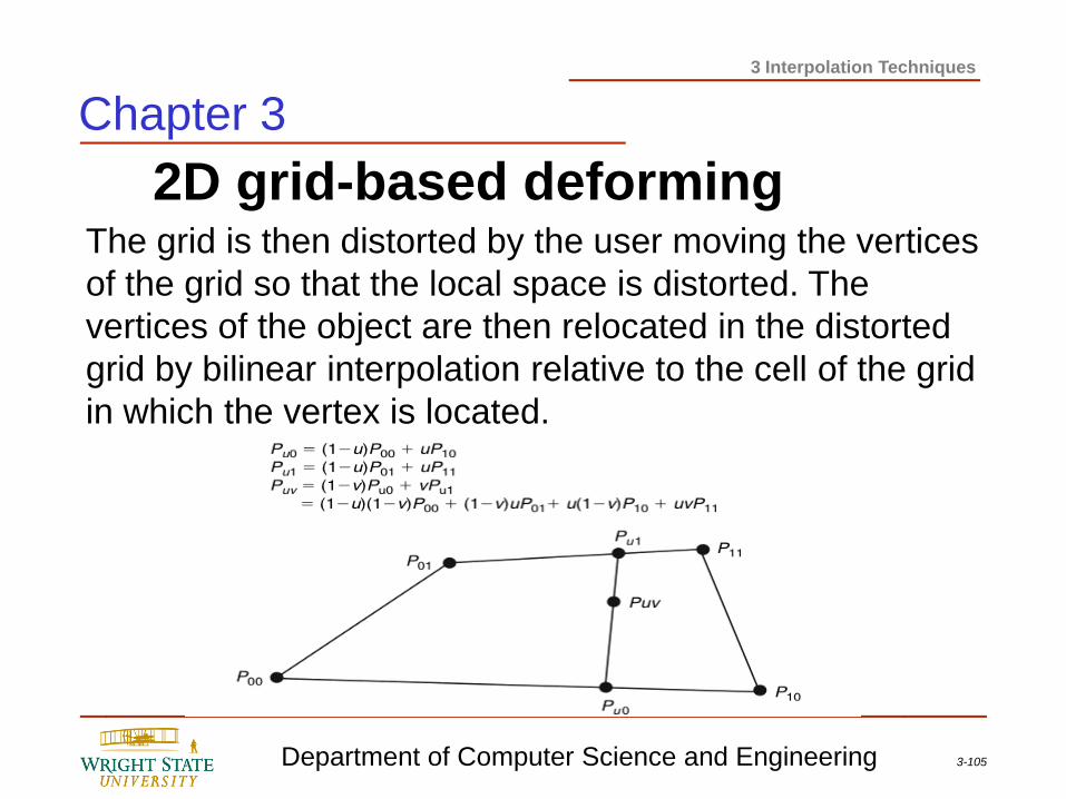
2D grid-based deforming The grid is then distorted by the user moving the vertices
of the grid so that the local space is distorted. The
vertices of the object are then relocated in the distorted
grid by bilinear interpolation relative to the cell of the grid
in which the vertex is located.
Chapter 3

3-106 Department of Computer Science and Engineering
3 Interpolation Techniques
2D grid-based deforming
Chapter 3
Once this is done for all vertices of the object, the object
is distorted according to the distortion of the local grid.
For the objects that contain hundreds of thousands of
vertices, the grid distortion is much more efficient than
individually repositioning each vertex. In addition, it is
more intuitive for the user to specify a deformation.
3-107 Department of Computer Science and Engineering
3 Interpolation Techniques
Chapter 3
Polyline Deformation Polyline deformation is similar to the grid approach in that the object
vertices are mapped to the polyline, the polyline is then modified by
the user, and the object vertices are then mapped to the same
relative location on the polyline.
The mapping to the polyline is performed by first locating the most
relevant line segment for each object vertex. To do this, intersecting
lines are formed at the junction of adjacent segments, and
perpendicular lines are formed at the extreme ends of the polyline.
These lines will be referred to as boundary lines; each polyline
segment has two boundary lines. For each object, the closest
polyline segment that contains the object vertex between its
boundary lines is selected.
3-108 Department of Computer Science and Engineering
3 Interpolation Techniques
2D Polyline Deformation
Chapter 3
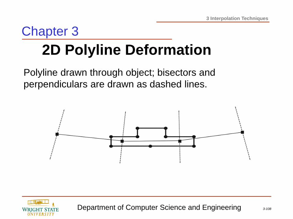
Polyline drawn through object; bisectors and
perpendiculars are drawn as dashed lines.
3-109 Department of Computer Science and Engineering
3 Interpolation Techniques
2D skeleton-based bending
Chapter 3
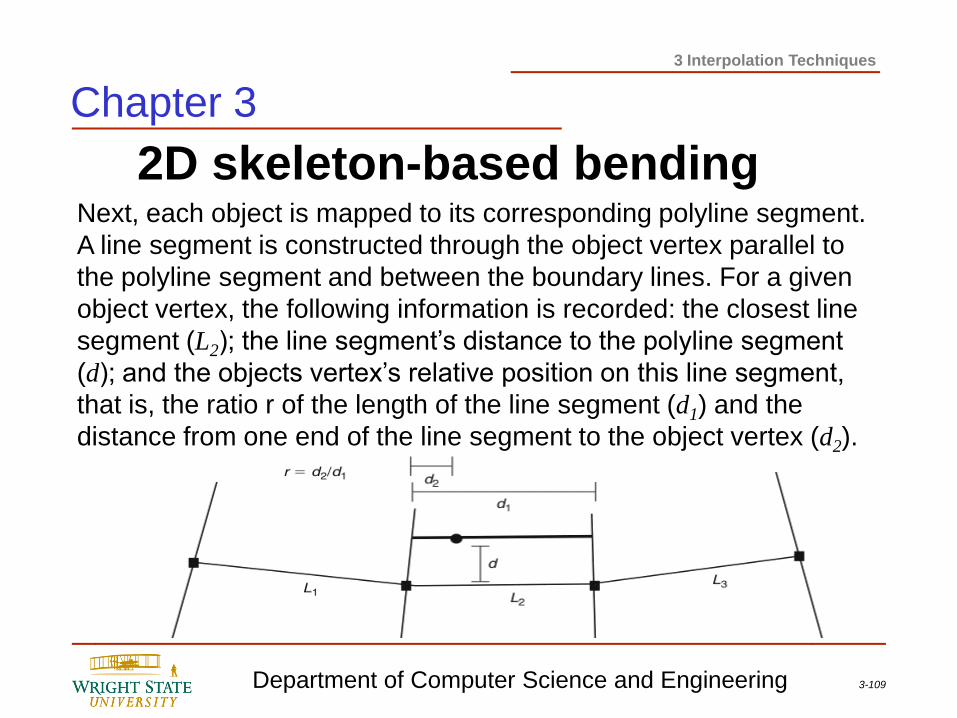
Next, each object is mapped to its corresponding polyline segment.
A line segment is constructed through the object vertex parallel to
the polyline segment and between the boundary lines. For a given
object vertex, the following information is recorded: the closest line
segment (L2); the line segment’s distance to the polyline segment
(d); and the objects vertex’s relative position on this line segment,
that is, the ratio r of the length of the line segment (d1) and the
distance from one end of the line segment to the object vertex (d2).
3-110 Department of Computer Science and Engineering
3 Interpolation Techniques
2D skeleton-based bending
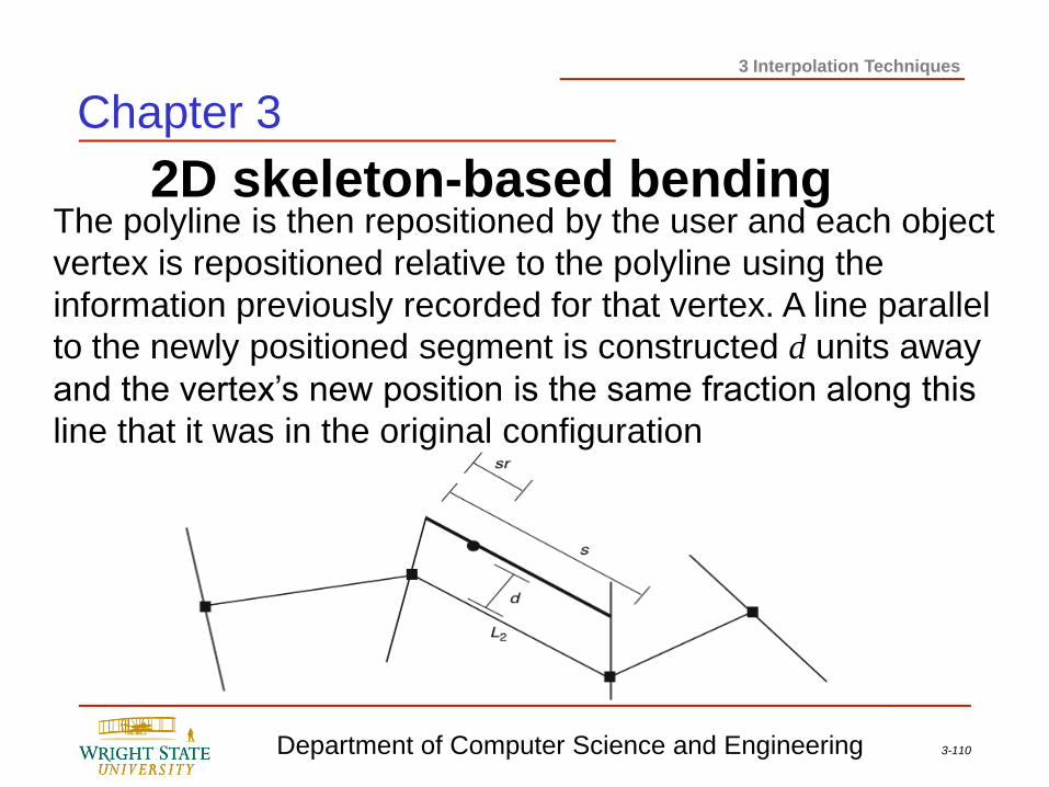
Chapter 3
The polyline is then repositioned by the user and each object
vertex is repositioned relative to the polyline using the
information previously recorded for that vertex. A line parallel
to the newly positioned segment is constructed d units away
and the vertex’s new position is the same fraction along this
line that it was in the original configuration
3-111 Department of Computer Science and Engineering
3 Interpolation Techniques
Global Transformations
ppMp )('
Mpp '
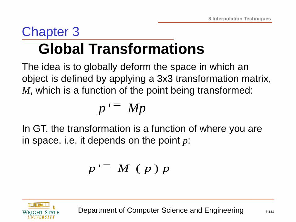
The idea is to globally deform the space in which an
object is defined by applying a 3x3 transformation matrix,
M, which is a function of the point being transformed:
In GT, the transformation is a function of where you are
in space, i.e. it depends on the point p:
Chapter 3
3-112 Department of Computer Science and Engineering
3 Interpolation Techniques
Global Transformations
Chapter 3
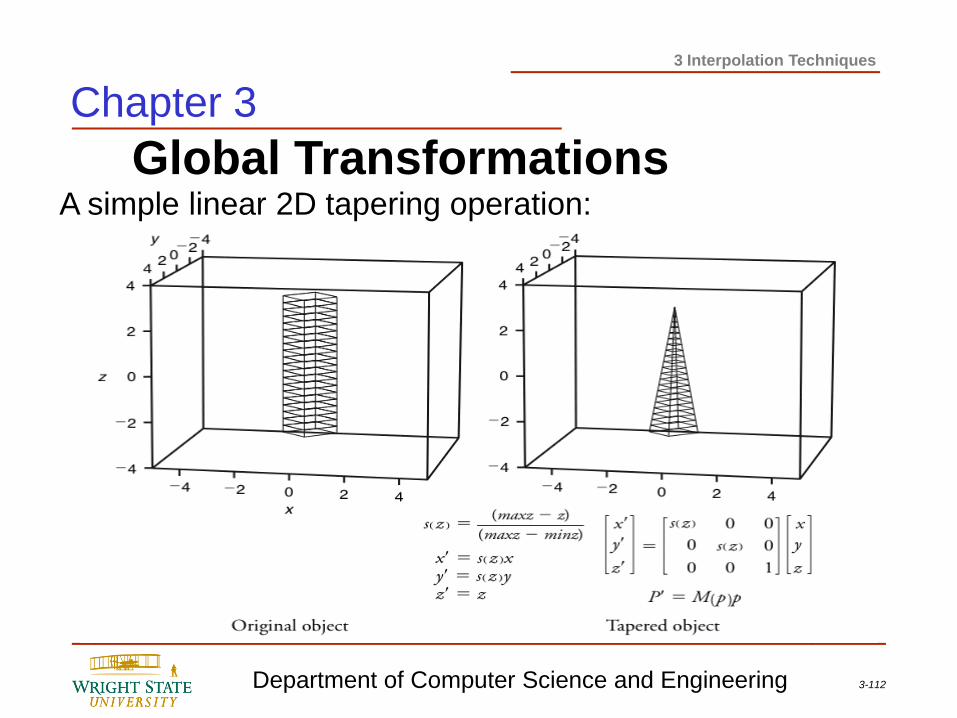
A simple linear 2D tapering operation:
3-113 Department of Computer Science and Engineering
3 Interpolation Techniques
Global Transformations
Chapter 3
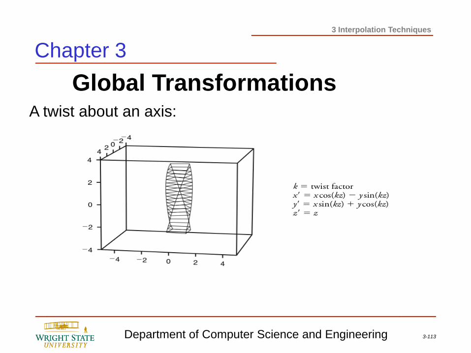
A twist about an axis:
3-114 Department of Computer Science and Engineering
3 Interpolation Techniques
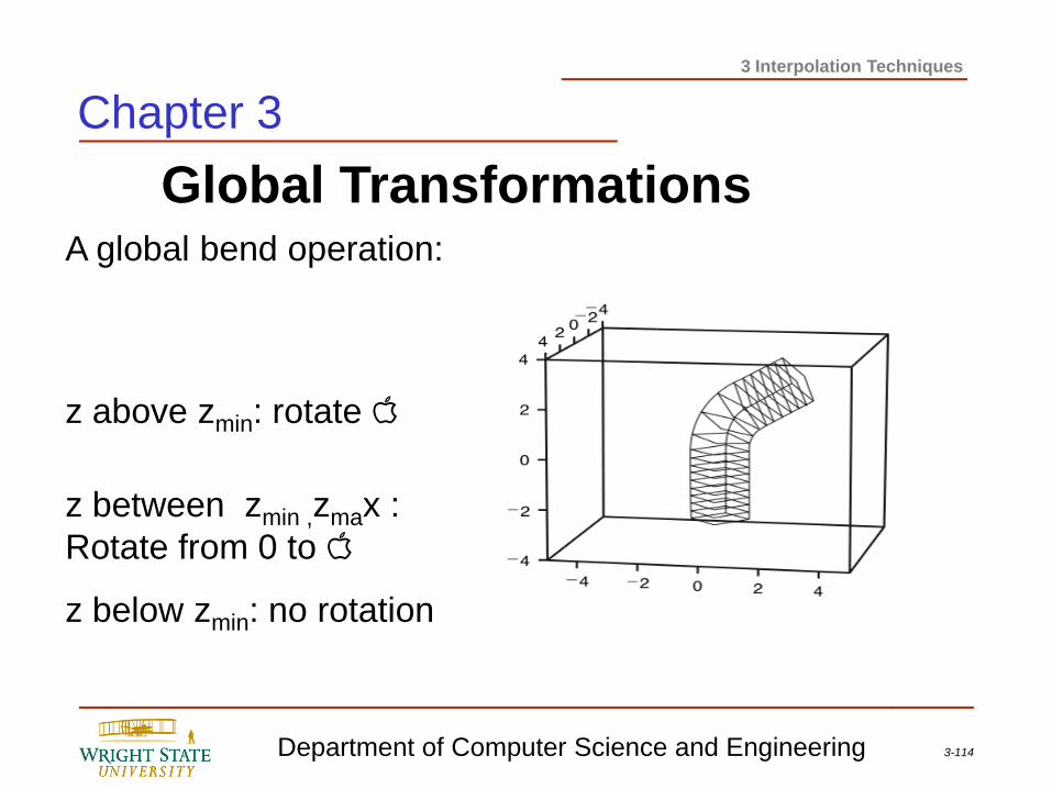
Global Transformations
z below zmin: no rotation
z between zmin ,zmax :
Rotate from 0 to Q
z above zmin: rotate Q
Chapter 3
A global bend operation:
3-115 Department of Computer Science and Engineering
3 Interpolation Techniques
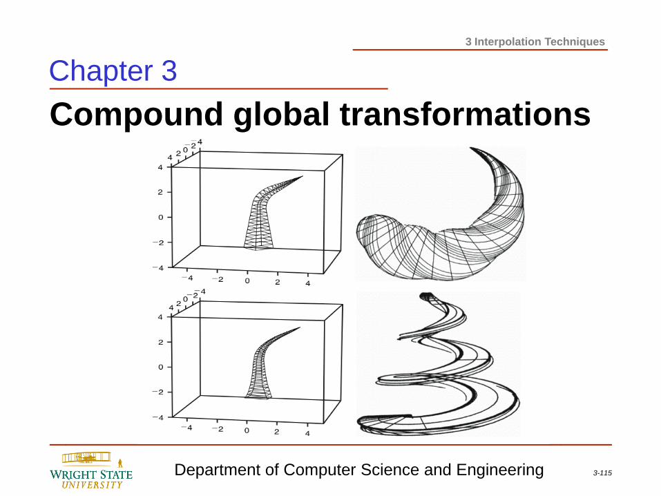
Compound global transformations
Chapter 3
3-116 Department of Computer Science and Engineering
3 Interpolation Techniques
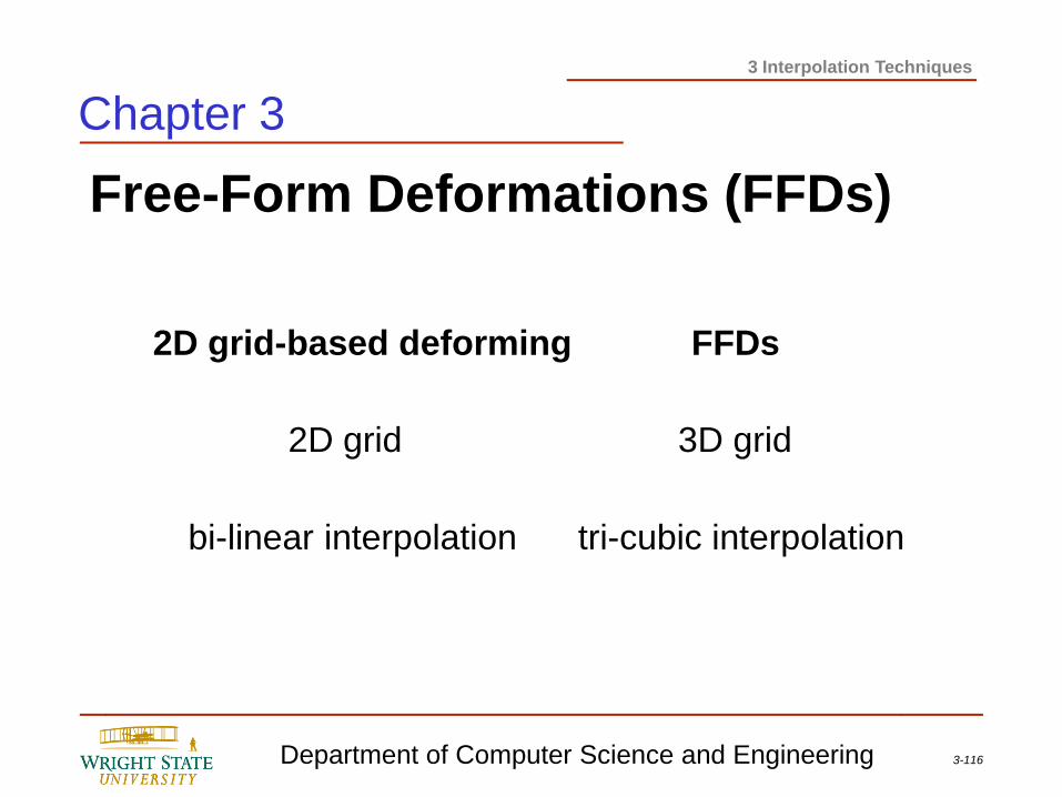
Free-Form Deformations (FFDs)
2D grid-based deforming FFDs
2D grid 3D grid
tri-cubic interpolation bi-linear interpolation
Chapter 3
3-117 Department of Computer Science and Engineering
3 Interpolation Techniques
Chapter 3
Free-Form Deformation
A Free-Form Deformation (FFD) is essentially a three-dimensional extension of Burtnyk’s grid deformation that incorporates higher-order interpolation. In both cases, a localized coordinate grid, in a standard configuration, is superimposed over an object. For each vertex of the object, coordinates relative to this local grid are determined that register the vertex to the grid. The grid is then manipulated by the user. Using its relative coordinates, each vertex is then mapped back into the modified grid, which relocates that vertex in global space. Instead of linear interpolation, cubic interpolation is typically used with FFDs, e.g. Bezier interpolation.
3-118 Department of Computer Science and Engineering
3 Interpolation Techniques
Free-Form Deformations
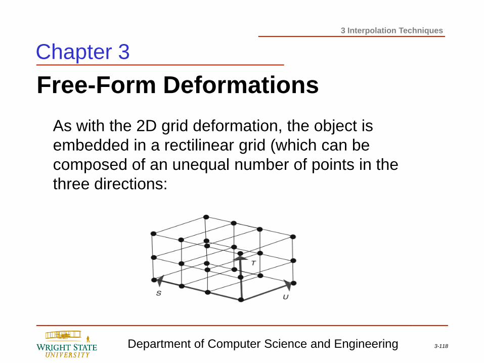
As with the 2D grid deformation, the object is
embedded in a rectilinear grid (which can be
composed of an unequal number of points in the
three directions:
Chapter 3
3-119 Department of Computer Science and Engineering
3 Interpolation Techniques
Free-Form Deformations
Chapter 3
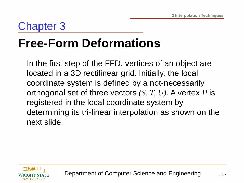
In the first step of the FFD, vertices of an object are
located in a 3D rectilinear grid. Initially, the local
coordinate system is defined by a not-necessarily
orthogonal set of three vectors (S, T, U). A vertex P is
registered in the local coordinate system by
determining its tri-linear interpolation as shown on the
next slide.
3-120 Department of Computer Science and Engineering
3 Interpolation Techniques
Free-Form Deformations
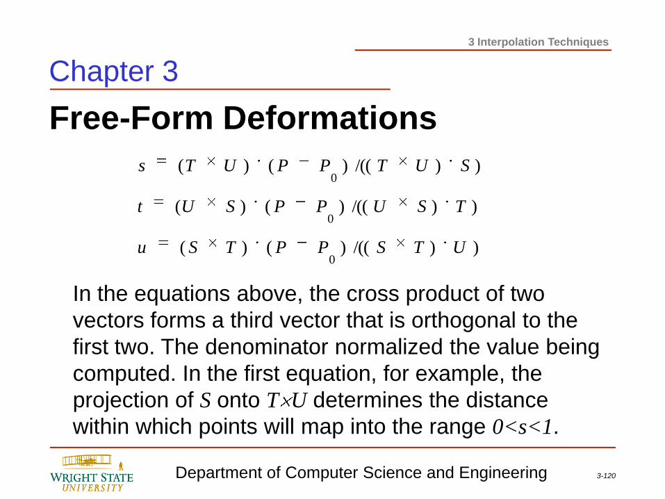
Chapter 3
In the equations above, the cross product of two
vectors forms a third vector that is orthogonal to the
first two. The denominator normalized the value being
computed. In the first equation, for example, the
projection of S onto T U determines the distance
within which points will map into the range 0<s<1.
))/(()()(
))/(()()(
))/(()()(
0
0
0
UTSPPTSu
TSUPPSUt
SUTPPUTs
3-121 Department of Computer Science and Engineering
3 Interpolation Techniques
Free-Form Deformations
Chapter 3
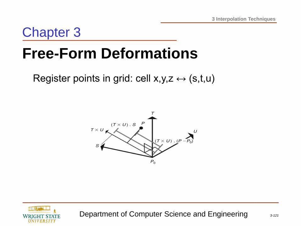
Register points in grid: cell x,y,z ↔ (s,t,u)
3-122 Department of Computer Science and Engineering
3 Interpolation Techniques
Free-Form Deformations
Chapter 3
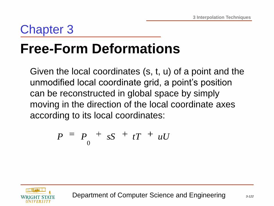
Given the local coordinates (s, t, u) of a point and the
unmodified local coordinate grid, a point’s position
can be reconstructed in global space by simply
moving in the direction of the local coordinate axes
according to its local coordinates:
uUtTsSPP0
3-123 Department of Computer Science and Engineering
3 Interpolation Techniques
Free-Form Deformations
Chapter 3
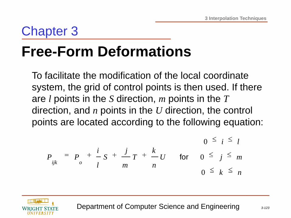
To facilitate the modification of the local coordinate
system, the grid of control points is then used. If there
are l points in the S direction, m points in the T
direction, and n points in the U direction, the control
points are located according to the following equation:
nk
mj
li
Un
kT
m
jS
l
iPP
oijk
0
0
0
for
3-124 Department of Computer Science and Engineering
3 Interpolation Techniques
Free-Form Deformations
Chapter 3
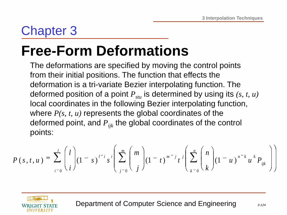
The deformations are specified by moving the control points
from their initial positions. The function that effects the
deformation is a tri-variate Bezier interpolating function. The
deformed position of a point Pstu is determined by using its (s, t, u)
local coordinates in the following Bezier interpolating function,
where P(s, t, u) represents the global coordinates of the
deformed point, and Pijk the global coordinates of the control
points:
ijk
kkn
n
k
jjm
m
j
iil
l
i
Puuk
ntt
j
mss
i
lutsP )1()1()1(),,(
000
3-125 Department of Computer Science and Engineering
3 Interpolation Techniques
Free-Form Deformations
Chapter 3
Show sample video.
3-126 Department of Computer Science and Engineering
3 Interpolation Techniques
Free-Form Deformations
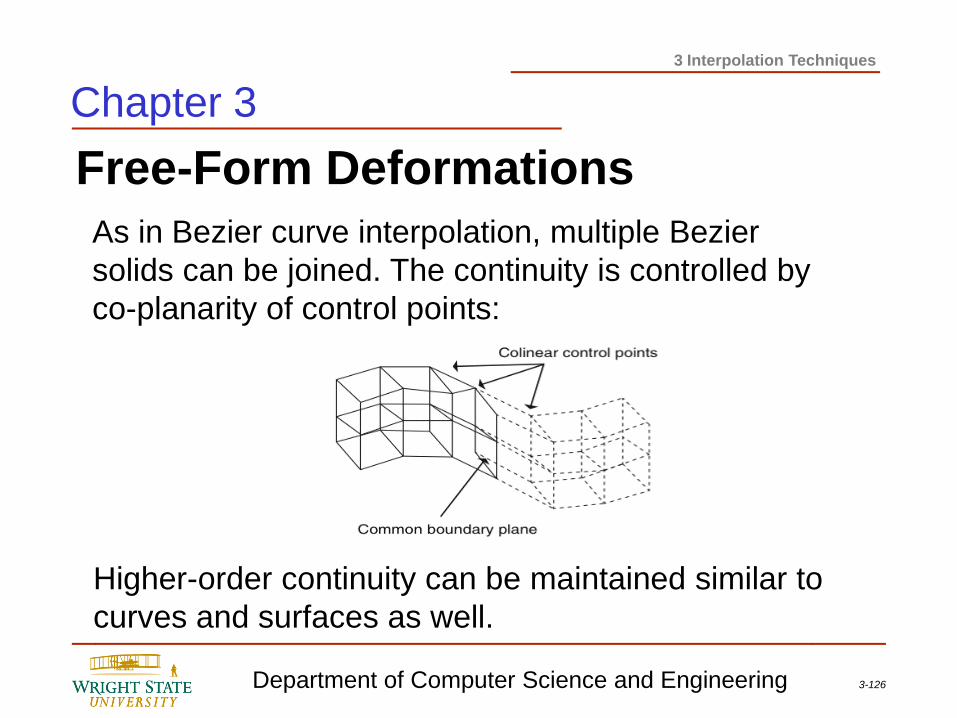
As in Bezier curve interpolation, multiple Bezier
solids can be joined. The continuity is controlled by
co-planarity of control points:
Chapter 3
Higher-order continuity can be maintained similar to
curves and surfaces as well.
3-127 Department of Computer Science and Engineering
3 Interpolation Techniques
FFDs: alternate grid organizations
Chapter 3
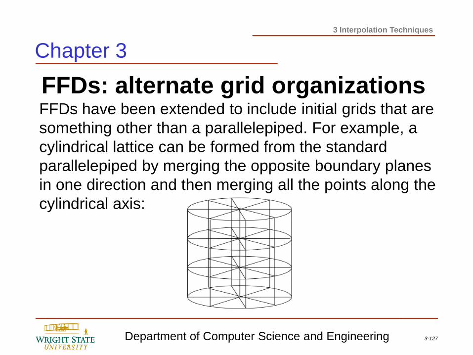
FFDs have been extended to include initial grids that are
something other than a parallelepiped. For example, a
cylindrical lattice can be formed from the standard
parallelepiped by merging the opposite boundary planes
in one direction and then merging all the points along the
cylindrical axis:
3-128 Department of Computer Science and Engineering
3 Interpolation Techniques
Composite FFDs
Chapter 3
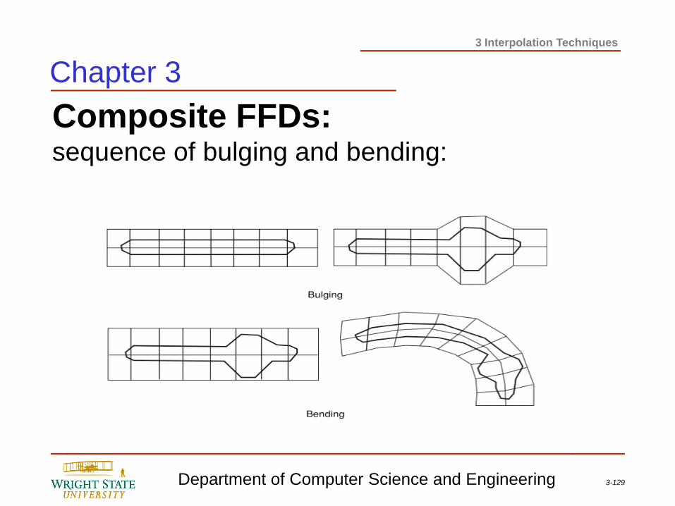
FFDs can be composed sequentially or hierarchically. In
a sequential composition, an object is modeled by
progressing through a sequence of FFDs, each of which
imparts a particular feature to the object. In this way,
various detail elements can be added to an object in
stages as opposed to trying to create one mammoth,
complex FFD designed to do everything at once. For
example, if a bulge is desired on a bent tube, then one
FFD can be used to impart the bulge while a second one
is designed to bend the object.
3-129 Department of Computer Science and Engineering
3 Interpolation Techniques
Composite FFDs: sequence of bulging and bending:
Chapter 3
3-130 Department of Computer Science and Engineering
3 Interpolation Techniques
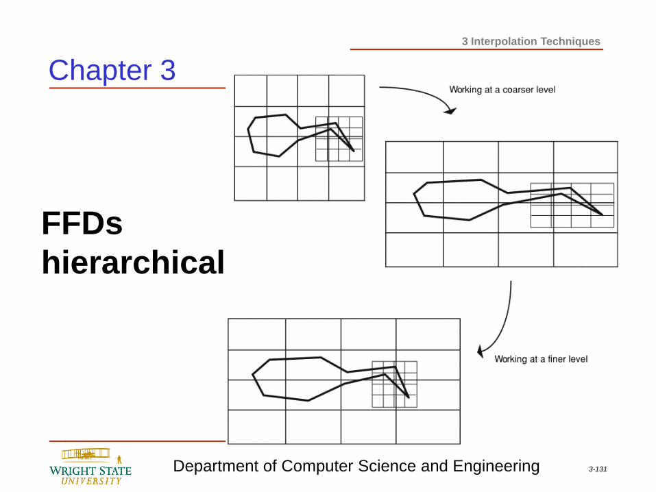
Hierarchical FFDs
Chapter 3
Organizing FFDs hierarchically allows the user to work at
various levels of detail. Finer resolution FFDs, usually
localized, are embedded inside FFDs higher in the
hierarchy. As a coarser-level FFD us used to modify the
object’s vertices, it also modifies the control points of any
of its children FFDs that are within the space affected by
the deformation. A modification made at a finer level in
the hierarchy will remain well defined even as the
animator works at a coarser level by modifying an FFD
grid higher up in the hierarchy.
3-131 Department of Computer Science and Engineering
3 Interpolation Techniques
FFDs
hierarchical
Chapter 3
3-132 Department of Computer Science and Engineering
3 Interpolation Techniques
Animated FFDs
Chapter 3
FFDs can also be used to control an animation in one of
two ways. The FFD can be constructed so that traversal
of an object through the FFD space results in a
continuous transformation of its shape. Alternatively, the
control points of an FFD can be animated, which results
in an animated deformation that automatically animates
the object’s shape.
3-133 Department of Computer Science and Engineering
3 Interpolation Techniques
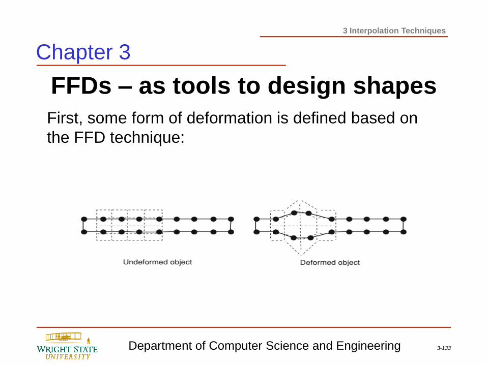
FFDs – as tools to design shapes
Chapter 3
First, some form of deformation is defined based on
the FFD technique:
3-134 Department of Computer Science and Engineering
3 Interpolation Techniques
Animated FFDs
Chapter 3
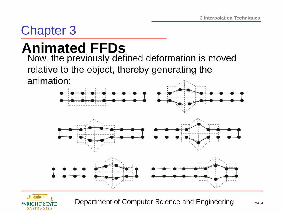
Now, the previously defined deformation is moved
relative to the object, thereby generating the
animation:
3-135 Department of Computer Science and Engineering
3 Interpolation Techniques
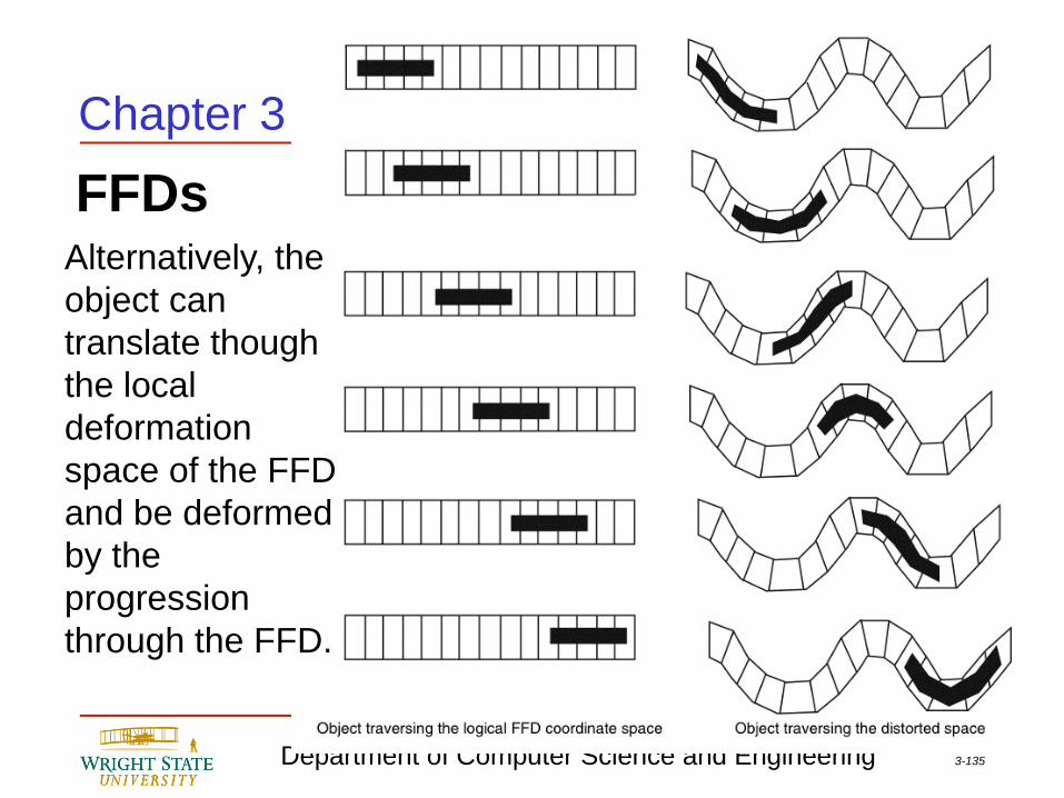
FFDs Alternatively, the
object can
translate though
the local
deformation
space of the FFD
and be deformed
by the
progression
through the FFD.
Chapter 3
3-136 Department of Computer Science and Engineering
3 Interpolation Techniques
Animated FFDs
Chapter 3
Another way to animate an object using FFDs is to
animate the control points of the FFD. For example, the
FFD control points can be animated explicitly using key-
frame animation, or their movement can be the result of a
physically-based simulation. As the FFD grid points
move, they define a changing deformation to be applied
to the object’s vertices.
3-137 Department of Computer Science and Engineering
3 Interpolation Techniques
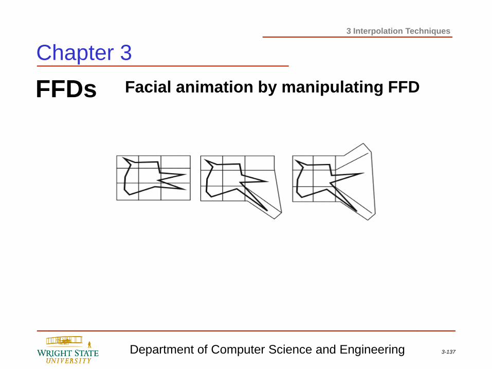
FFDs Facial animation by manipulating FFD
Chapter 3
3-138 Department of Computer Science and Engineering
3 Interpolation Techniques
Animated FFDs
Chapter 3
FFDs can also be used to model muscles of a human
model. The muscles in this case are not meant to be
anatomical representations of real muscles but to provide
for a more artistic style.
As a simple example, a hinge joint with adjacent links is
modeled. There are three FFDs: one for each of the two
links and one for the joint. The FFDs associated with the
links will deform the skin according to a stylized muscle,
and the purpose of the FFD associated with the joint is to
prevent interpenetration of the skin surface in highly bent
configurations:
3-139 Department of Computer Science and Engineering
3 Interpolation Techniques
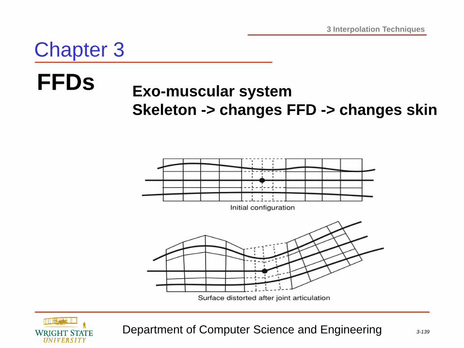
FFDs Exo-muscular system
Skeleton -> changes FFD -> changes skin
Chapter 3
3-140 Department of Computer Science and Engineering
3 Interpolation Techniques
Animated FFD
Show sample video.
Chapter 3
3-141 Department of Computer Science and Engineering
3 Interpolation Techniques
Chapter 3
3D Shape Interpolation
We first need to define a few terms:
topology (mathematical):
Describes the connectivity of the surface of an object,
i.e. the number of holes and the number of separate
bodies
genus:
Number of holes of an object
topology (computer graphics):
Vertex/edge/face connectivity of an object
3-142 Department of Computer Science and Engineering
3 Interpolation Techniques
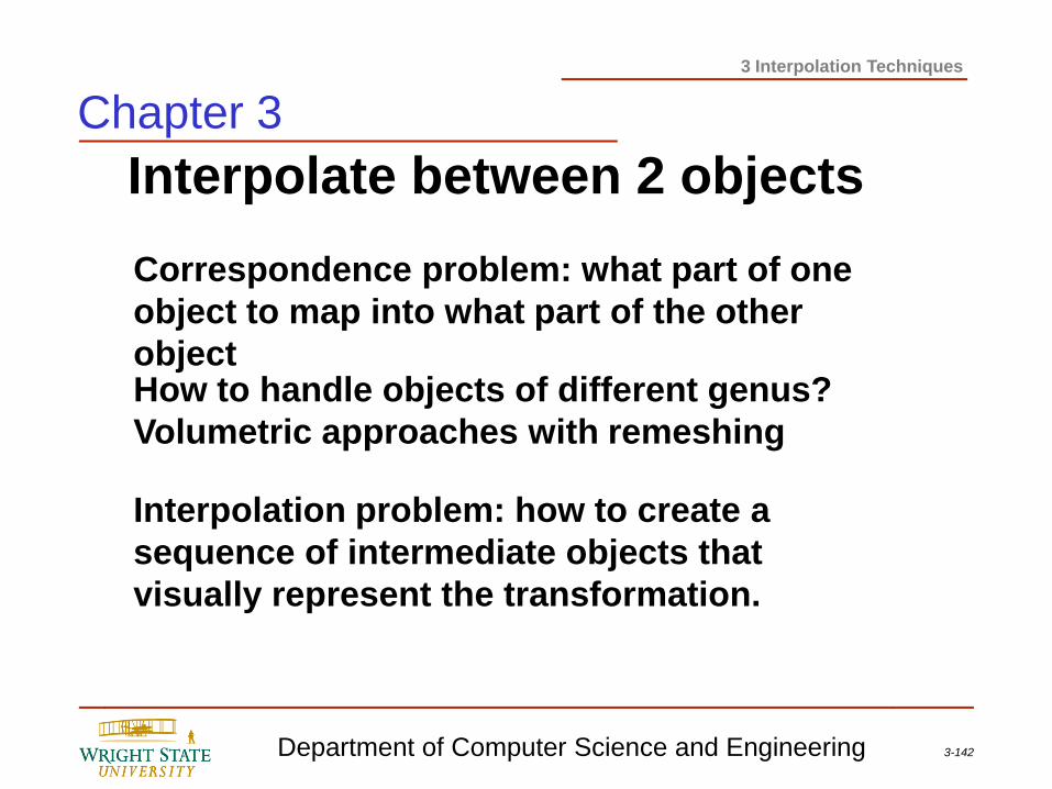
Interpolate between 2 objects
Correspondence problem: what part of one
object to map into what part of the other
object
Interpolation problem: how to create a
sequence of intermediate objects that
visually represent the transformation.
How to handle objects of different genus?
Volumetric approaches with remeshing
Chapter 3
3-143 Department of Computer Science and Engineering
3 Interpolation Techniques
Chapter 3
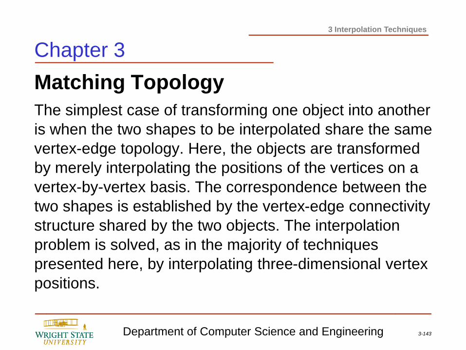
Matching Topology
The simplest case of transforming one object into another
is when the two shapes to be interpolated share the same
vertex-edge topology. Here, the objects are transformed
by merely interpolating the positions of the vertices on a
vertex-by-vertex basis. The correspondence between the
two shapes is established by the vertex-edge connectivity
structure shared by the two objects. The interpolation
problem is solved, as in the majority of techniques
presented here, by interpolating three-dimensional vertex
positions.
3-144 Department of Computer Science and Engineering
3 Interpolation Techniques
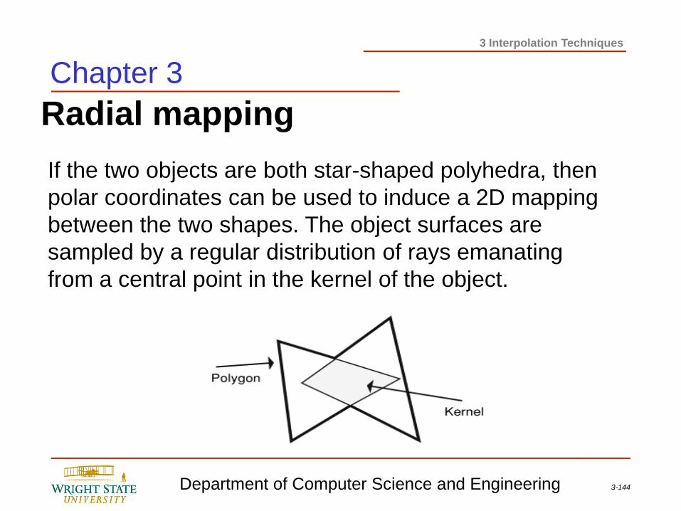
Radial mapping
If the two objects are both star-shaped polyhedra, then
polar coordinates can be used to induce a 2D mapping
between the two shapes. The object surfaces are
sampled by a regular distribution of rays emanating
from a central point in the kernel of the object.
Chapter 3
3-145 Department of Computer Science and Engineering
3 Interpolation Techniques
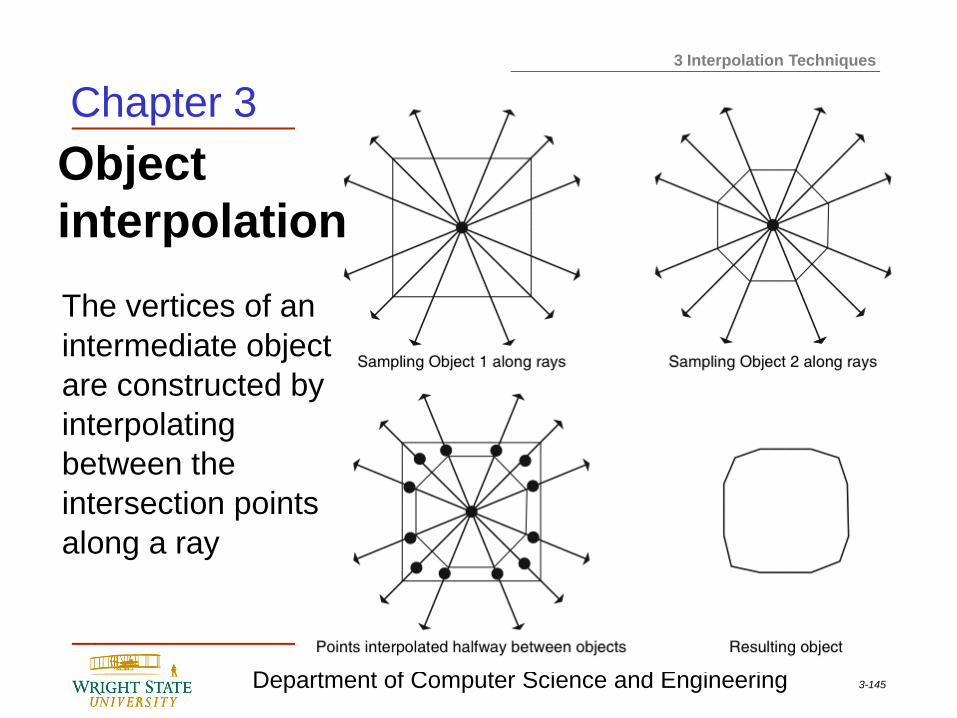
Object
interpolation
Chapter 3
The vertices of an
intermediate object
are constructed by
interpolating
between the
intersection points
along a ray
3-146 Department of Computer Science and Engineering
3 Interpolation Techniques
Chapter 3
Axial Slices
The idea can be extended to 3D objects as well. For each
object, the user defines an axis that runs through the
middle of the object. At regular intervals along this axis,
perpendicular slices are taken of an object. These slices
must be star shaped with respect to the point of
intersection between the axis and the slice. This central
axis is defined for both objects, and the part of each axis
interior to its respective object is parameterized from zero
to one. In addition, the user defines an orientation vector
(or a default direction is used) that is perpendicular to the
axis.
3-147 Department of Computer Science and Engineering
3 Interpolation Techniques
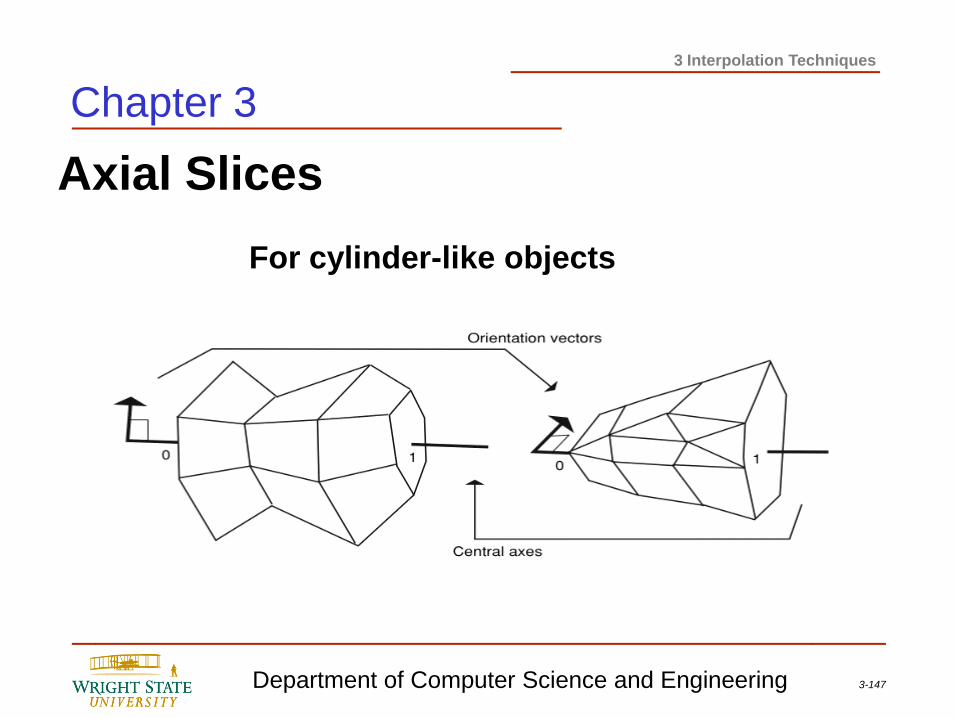
Axial Slices
For cylinder-like objects
Chapter 3
3-148 Department of Computer Science and Engineering
3 Interpolation Techniques
Chapter 3
Axial Slices
Corresponding slices (in the sense that they use the
same axis parameter to define the plane of intersection)
are taken from each object. The two-dimensional slices
can be interpolated pair-wise (one from each object) by
constructing rays that emanate from the center point and
sample the boundary at regular intervals with respect to
the orientation vector.
3-149 Department of Computer Science and Engineering
3 Interpolation Techniques
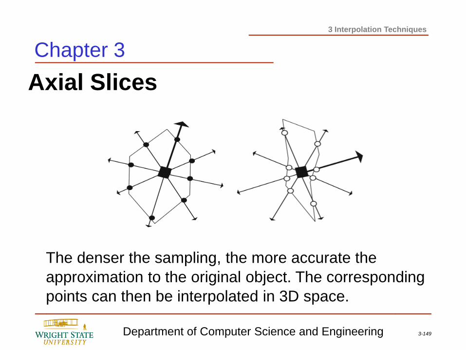
Axial Slices
Chapter 3
The denser the sampling, the more accurate the
approximation to the original object. The corresponding
points can then be interpolated in 3D space.
3-150 Department of Computer Science and Engineering
3 Interpolation Techniques
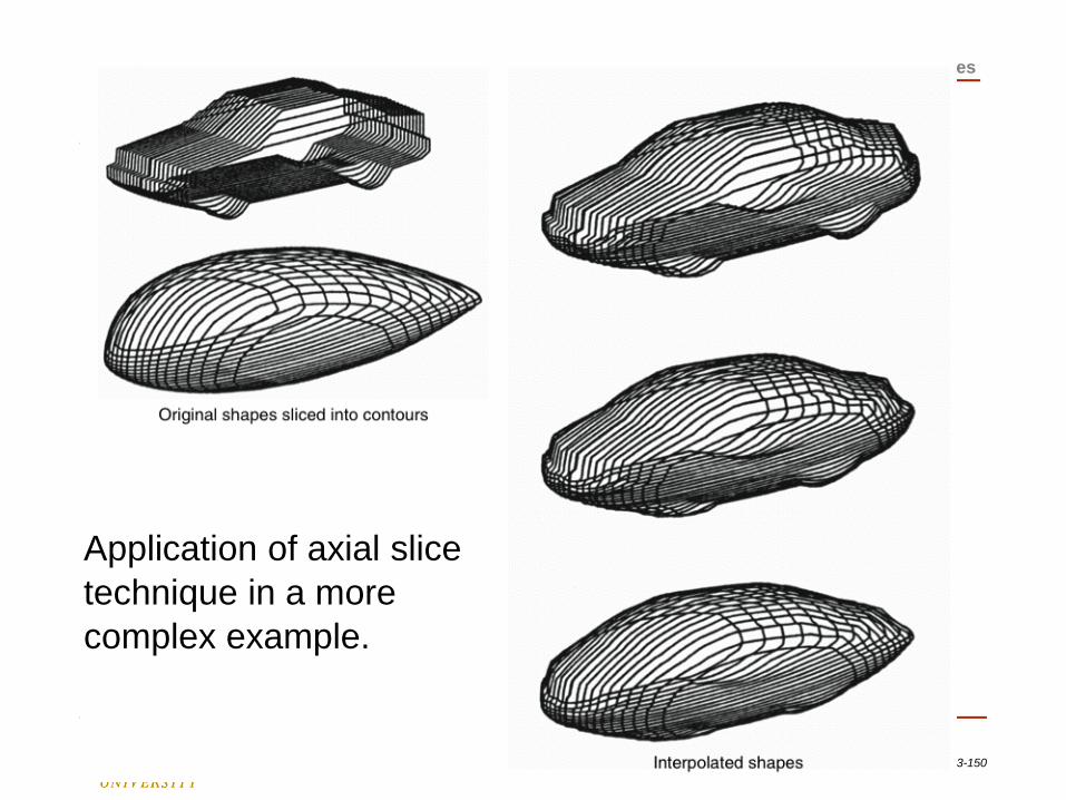
Application of axial slice
technique in a more
complex example.
3-151 Department of Computer Science and Engineering
3 Interpolation Techniques
Chapter 3
Object Interpolation Even among genus 0 objects, more complex polyhedra may not be star shaped or allow an internal axis to define star-shaped slices. A more complicated mapping procedure may be required to establish the 2D parameterization of the object’s surfaces. One approach is to map both objects onto a common surface, such as a unit sphere. The mapping must be such that the entire object surface maps to the entire sphere with no overlap. Once both objects have been mapped onto the sphere, a union of their vertex-edge topologies can be constructed and then inversely mapped back onto each original object.
3-152 Department of Computer Science and Engineering
3 Interpolation Techniques
Chapter 3
Object Interpolation
If both objects are successfully mapped to the sphere’s
surface, the projected edges are intersected and merged
into one topology. The new vertices and edges are a
superset of both object topologies. They are then
projected back onto both object surfaces. This produces
two new object definitions, identical in shape to the original
objects but now having the same vertex-edge topology,
allowing for a vertex-by-vertex interpolation to transform
one object into the other.
3-153 Department of Computer Science and Engineering
3 Interpolation Techniques
Object interpolation
1. Map to sphere
2. Intersect arc-edges
3. Retriangulate
4. Remap to object shapes
5. Vertex-to-vertex interpolation
Spherical mapping to establish
matching edge-vertex topology
Chapter 3
3-154 Department of Computer Science and Engineering
3 Interpolation Techniques
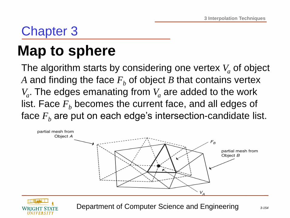
Map to sphere
Chapter 3
The algorithm starts by considering one vertex Va of object
A and finding the face Fb of object B that contains vertex
Va. The edges emanating from Va are added to the work
list. Face Fb becomes the current face, and all edges of
face Fb are put on each edge’s intersection-candidate list.
3-155 Department of Computer Science and Engineering
3 Interpolation Techniques
Chapter 3
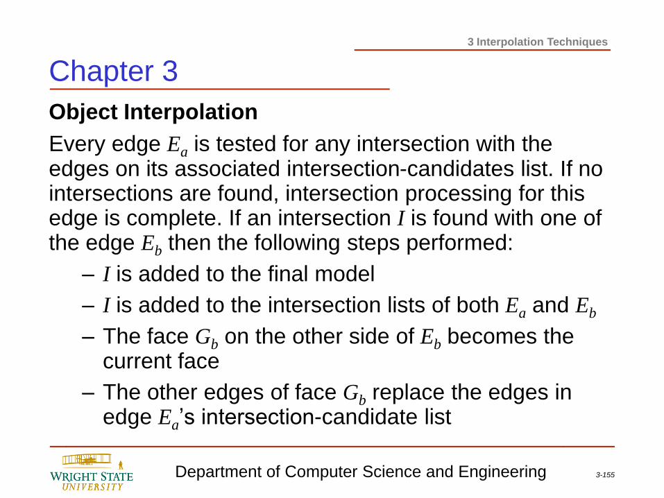
Object Interpolation
Every edge Ea is tested for any intersection with the edges on its associated intersection-candidates list. If no intersections are found, intersection processing for this edge is complete. If an intersection I is found with one of the edge Eb then the following steps performed:
– I is added to the final model
– I is added to the intersection lists of both Ea and Eb
– The face Gb on the other side of Eb becomes the current face
– The other edges of face Gb replace the edges in edge Ea’s intersection-candidate list
3-156 Department of Computer Science and Engineering
3 Interpolation Techniques
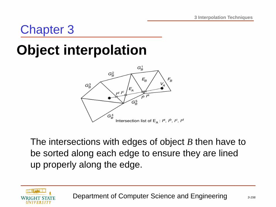
Object interpolation
Chapter 3
The intersections with edges of object B then have to
be sorted along each edge to ensure they are lined
up properly along the edge.
3-157 Department of Computer Science and Engineering
3 Interpolation Techniques
Chapter 3
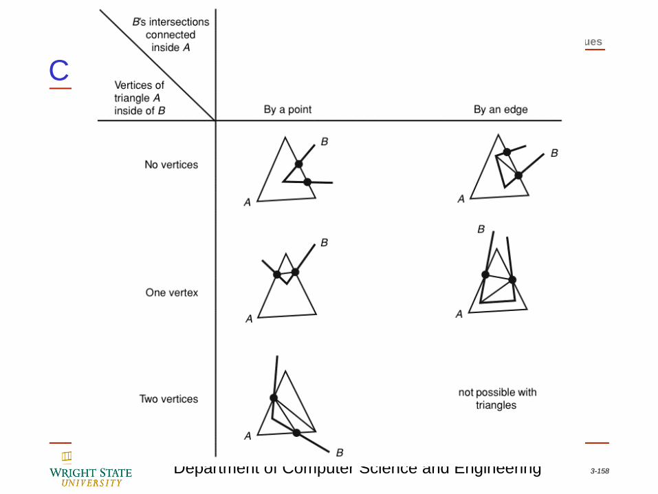
Object Interpolation
Now, all the vertices, edges, and intersection points are
mapped back onto the original objects. New face
definitions need to be constructed for each object.
Because both models started out as triangulated meshes,
there are only a limited number of configurations possible
when one considers the triangulation required from the
combined models.
3-158 Department of Computer Science and Engineering
3 Interpolation Techniques
Chapter 3
3-159 Department of Computer Science and Engineering
3 Interpolation Techniques
Chapter 3
Object Interpolation
After this process, both objects have the same topology
so that we can easily interpolate between the two by
linearly interpolating between the vertices of both objects.
3-160 Department of Computer Science and Engineering
3 Interpolation Techniques
Chapter 3
Object Interpolation
The main problem with the previous procedure is that
many new edges are created as a result of the merging
operation. There is no attempt to map existing edges into
one another. To avoid a plethora of new edges, a
recursive approach can be taken in which each object is
reduced to 2D polygonal meshes. Meshes from each
object are matched by associating the boundary vertices
and adding new ones when necessary. The meshes are
then similarly split and the procedure is recursively
applied until everything has been reduced to triangles.
3-161 Department of Computer Science and Engineering
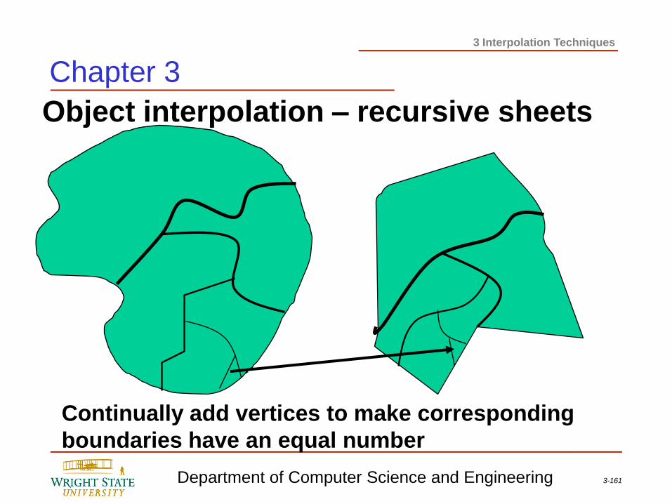
3 Interpolation Techniques
Object interpolation – recursive sheets
Continually add vertices to make corresponding
boundaries have an equal number
Chapter 3
3-162 Department of Computer Science and Engineering
3 Interpolation Techniques
Chapter 3
Object Interpolation
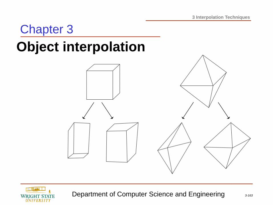
The initial objects are divided into an initial number of
polygonal meshes. Each mesh is associated with a mesh
from the other object so that adjacency relationships are
maintained by the mapping. The simplest way to do this
is merely to break each object into two meshes: a front
mesh and a back mesh. A front and back mesh can be
constructed by searching for the shortest paths between
the topmost, bottommost, leftmost, and rightmost vertices
of the object and then appending these paths:
3-163 Department of Computer Science and Engineering
3 Interpolation Techniques
Object interpolation
Chapter 3
3-164 Department of Computer Science and Engineering
3 Interpolation Techniques
Chapter 3
Object Interpolation
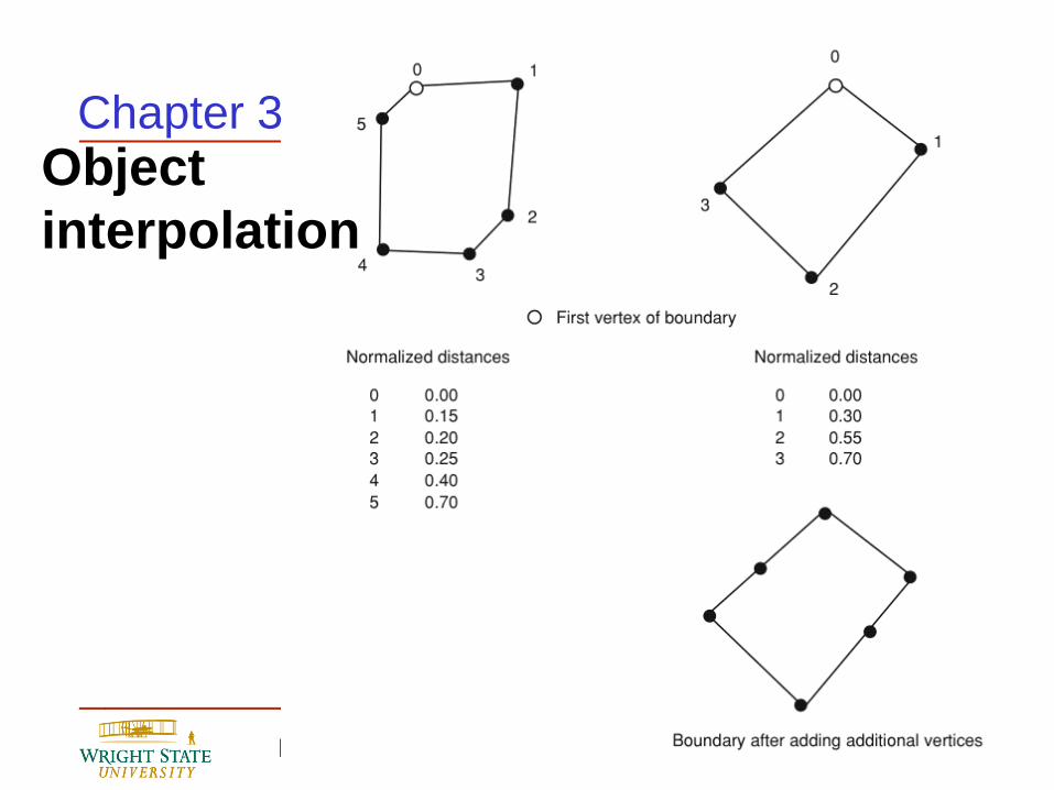
If one of the meshes has fewer boundary vertices than
the other, then new vertices must be introduced along its
boundary to make up for the difference. There are various
ways to do this, and the success of the algorithm is not
dependent on the method. A suggested method is to
compute the normalized distances of each vertex along
the boundary as measured from the first vertex of the
boundary. For the boundary with fewer vertices, new
vertices can be added one at a time by searching for the
largest gap in normalized distances for successive
vertices in the boundary:
3-165 Department of Computer Science and Engineering
3 Interpolation Techniques
Object
interpolation
Chapter 3
3-166 Department of Computer Science and Engineering
3 Interpolation Techniques
Chapter 3
Object Interpolation
When the boundaries have the same number of vertices,
a vertex on one boundary is said to be associated with
the vertex on the other boundary at the same relative
location. Once the meshes have been associated, each
mesh is recursively divided. One mesh is chosen for
division, and a path of edges is found across it. One good
approach for this is to choose two vertices across the
boundary from each other and try to find an existing path
of edges between them.
3-167 Department of Computer Science and Engineering
3 Interpolation Techniques
Chapter 3
Object Interpolation
Once a path has been found across one mesh, then a path across the mesh it is associated with must be established between corresponding vertices. This may require creating new vertices and new edges. When these paths have been created, the meshes can be divided along these paths, creating two pairs of new meshes. The boundary association, finding a path of edges, and mesh splitting are recursively applied to each new mesh until all of the meshes have been reduced to single triangles. At this point the new vertices and new edges have been added to one or both objects so that both objects have the same topology.
3-168 Department of Computer Science and Engineering
3 Interpolation Techniques
Morphing
Image blending
Move pixels to corresponding pixels
Blend colors
Chapter 3
3-169 Department of Computer Science and Engineering
3 Interpolation Techniques
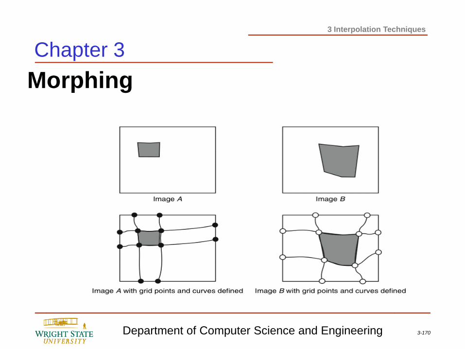
Chapter 3
Morphing To transform one image into another, the user defines a curvilinear grid over each of the two images to be morphed. It is the user’s responsibility to define the grids so that corresponding elements in the images are in the corresponding cells of the grids. The user defines the grid by locating the same number of grid intersection points in both images; the grid must be defined at the borders of the images in order to include the entire image. A curved mesh is then generated using the grid intersection points as control points for an interpolation scheme, such as Catmull-Rom or Bezier splines.
3-170 Department of Computer Science and Engineering
3 Interpolation Techniques
Morphing
Chapter 3
3-171 Department of Computer Science and Engineering
3 Interpolation Techniques
Chapter 3
Morphing
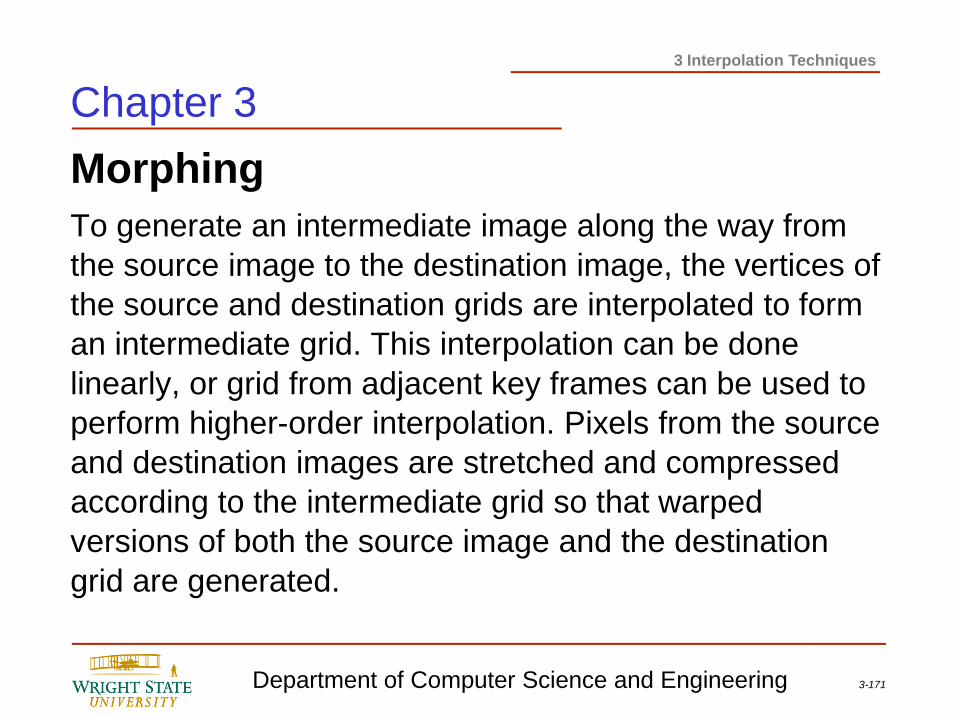
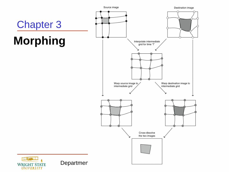
To generate an intermediate image along the way from
the source image to the destination image, the vertices of
the source and destination grids are interpolated to form
an intermediate grid. This interpolation can be done
linearly, or grid from adjacent key frames can be used to
perform higher-order interpolation. Pixels from the source
and destination images are stretched and compressed
according to the intermediate grid so that warped
versions of both the source image and the destination
grid are generated.
3-172 Department of Computer Science and Engineering
3 Interpolation Techniques
Morphing
Chapter 3
3-173 Department of Computer Science and Engineering
3 Interpolation Techniques
Chapter 3
Morphing
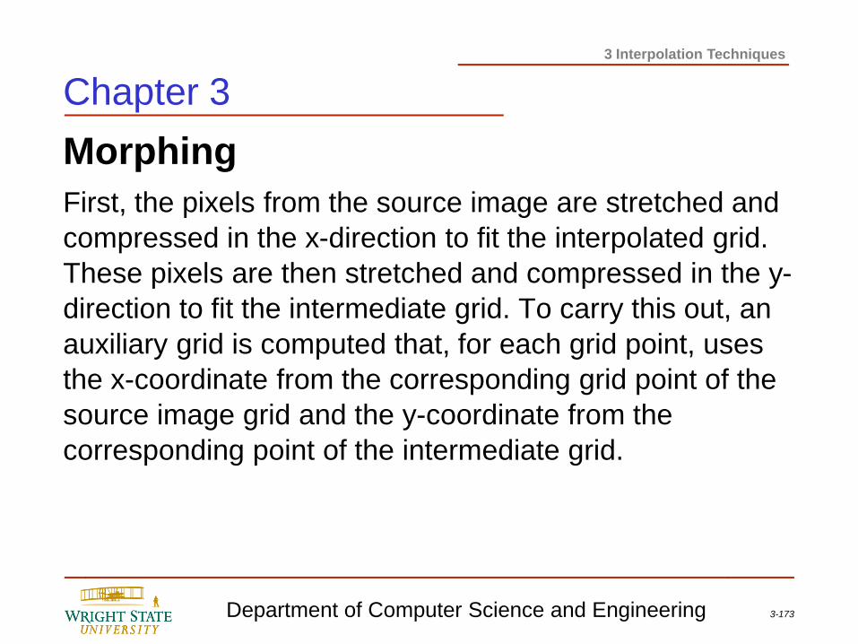
First, the pixels from the source image are stretched and
compressed in the x-direction to fit the interpolated grid.
These pixels are then stretched and compressed in the y-
direction to fit the intermediate grid. To carry this out, an
auxiliary grid is computed that, for each grid point, uses
the x-coordinate from the corresponding grid point of the
source image grid and the y-coordinate from the
corresponding point of the intermediate grid.
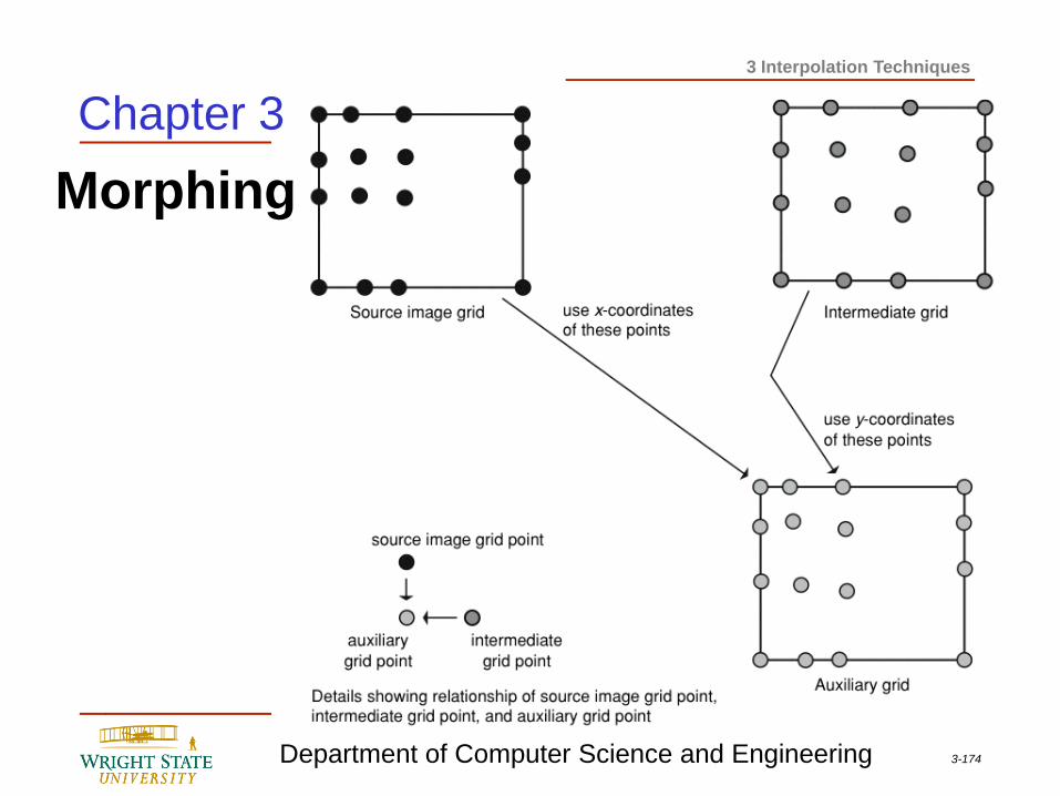
3-174 Department of Computer Science and Engineering
3 Interpolation Techniques
Chapter 3
Morphing
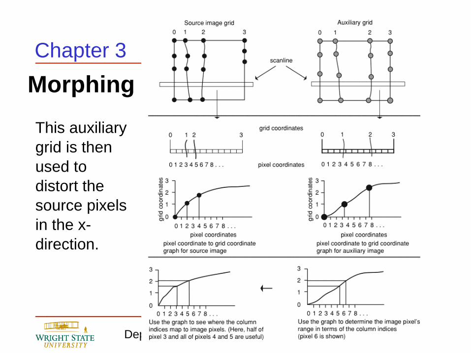
3-175 Department of Computer Science and Engineering
3 Interpolation Techniques
Morphing
Chapter 3
This auxiliary
grid is then
used to
distort the
source pixels
in the x-
direction.
3-176 Department of Computer Science and Engineering
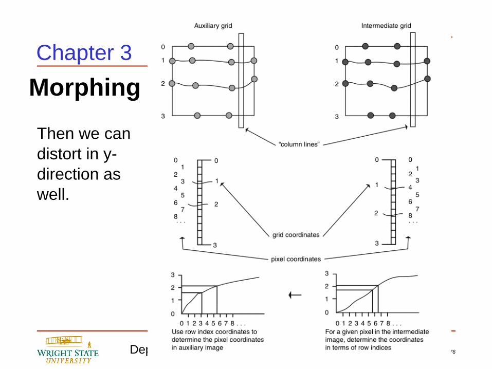
3 Interpolation Techniques
Morphing
Chapter 3
Then we can
distort in y-
direction as
well.
3-177 Department of Computer Science and Engineering
3 Interpolation Techniques
Morphing
Chapter 3
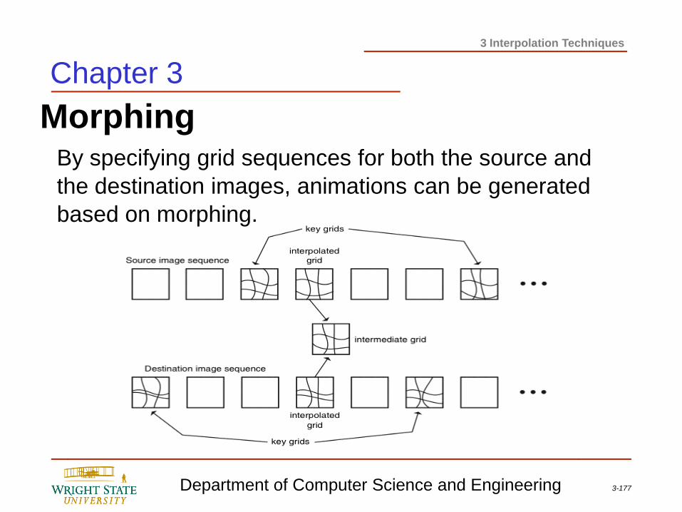
By specifying grid sequences for both the source and
the destination images, animations can be generated
based on morphing.
3-178 Department of Computer Science and Engineering
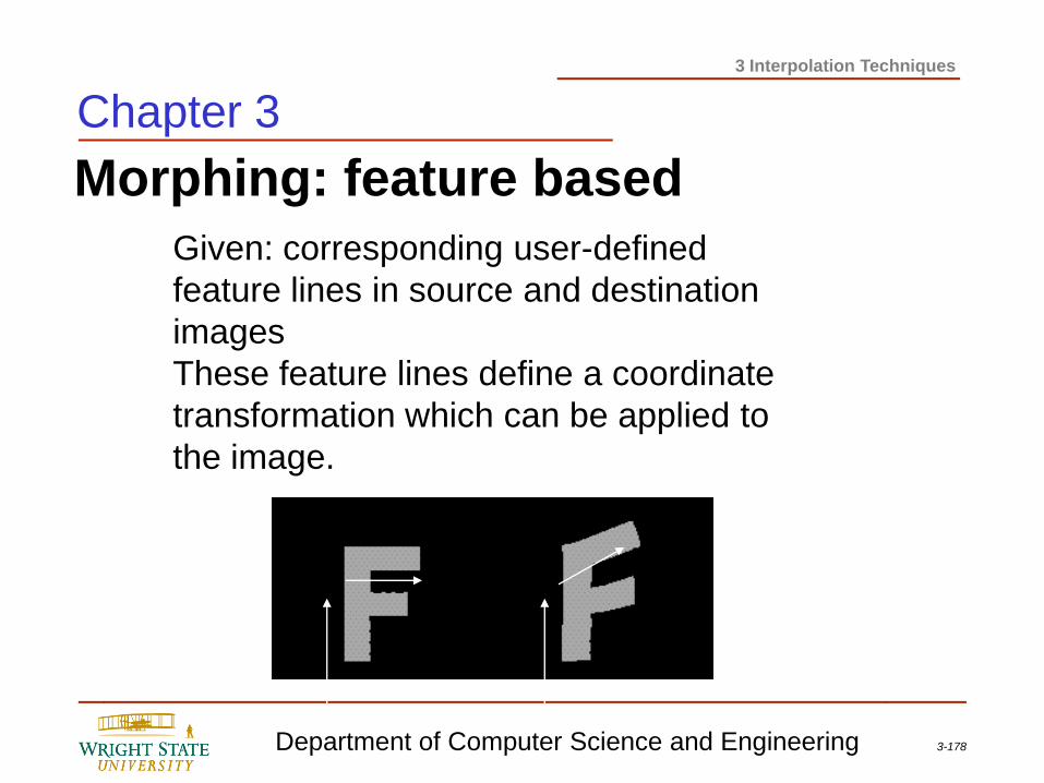
3 Interpolation Techniques
Morphing: feature based
Given: corresponding user-defined
feature lines in source and destination
images
These feature lines define a coordinate
transformation which can be applied to
the image.
Chapter 3
3-179 Department of Computer Science and Engineering
3 Interpolation Techniques
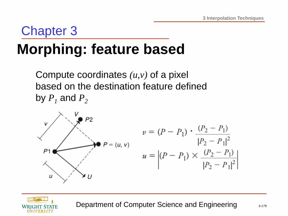
Morphing: feature based
Compute coordinates (u,v) of a pixel
based on the destination feature defined
by P1 and P2
Chapter 3
3-180 Department of Computer Science and Engineering
3 Interpolation Techniques
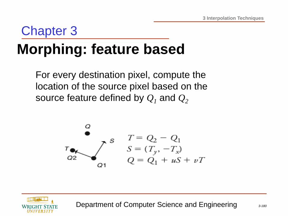
Morphing: feature based
Chapter 3
For every destination pixel, compute the
location of the source pixel based on the
source feature defined by Q1 and Q2
3-181 Department of Computer Science and Engineering
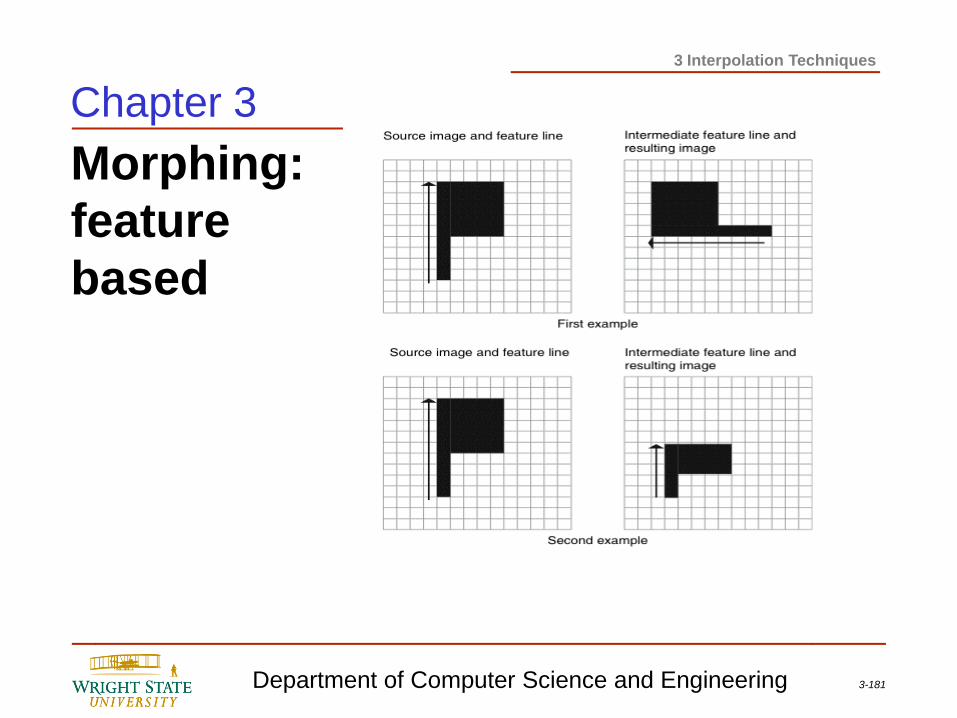
3 Interpolation Techniques
Morphing:
feature
based
Chapter 3
3-182 Department of Computer Science and Engineering
3 Interpolation Techniques
Chapter 3
Morphing video that illustrates 3D facial animation