Model-Checking Techniques and Tools

S d S f V ifi iSystems and Software VerificationModel-Checking Techniques and Tools

JUNBEOM YOOJUNBEOM YOO

Dependable Software LaboratoryKONKUK University

http://dslab.konkuk.ac.kr

Ver. 2.5 (2013.06)

IntroductionIntroduction

T• Text– System and Software Verification : Model-Checking Techniques and Tools

• In this book, you will find enough theory– to be able to assess the relevance of the various tools,– to understand the reasons behind their limitations and strengths, and– to choose the approach currently best suited for your verification task.

• Part I : Principles and Techniques• Part II : Specifying with Temporal Logic• Part II : Specifying with Temporal Logic• Part III : Some Tools

Dependable Software Laboratory 2

Chapter 1 AutomataChapter 1. Automata

M d l h ki i t i if i ti f th d l f• Model checking consists in verifying some properties of the model of a system.

• Modeling of a system is difficultNo universal method exists to model a system– No universal method exists to model a system

– Best performed by qualified engineers

• This chapter describes a general model which serves as a basis.This chapter describes a general model which serves as a basis.

• Organization of Chapter 1– Introductory Examplesy p– A Few Definitions– A Printer Manager– A Few More Variables

Synchronized Product– Synchronized Product– Synchronization with Messaging Passing– Synchronization by Shared Variables


1 1 Introductory Examples1.1 Introductory Examples

(Fi i ) A• (Finite) Automata– Best suited for verification by model checking techniques– A machine evolving from one state to another under the action of transitions

Graphical representation– Graphical representation

03:58… 03:59 04:00 …03:58 03:59 04:00

An automate model of a digital watch (24x60=1440 states)


dec

0 1inc

dec inc

decinc

2

Ac3 : a module 3 counter


• A digicode door lock example– Controls the opening of office doors

The door opens upon the keying in of the correct character sequence irrespective of any– The door opens upon the keying in of the correct character sequence, irrespective of any possible incorrect initial attempts.

– Assumes• 3 keys A, B, and C• Correct key sequence : ABA

AB , C

1 2 3 4AB

A

CC

B CB , C


• Two fundamental notationsi– execution

• A sequence of states describing one possible evolution of the system• Ex. 1121 , 12234 , 112312234 3 different executions

execution tree– execution tree• A set of all possible executions of the system in the form of a tree• Ex. 1

11, 12111, 112, 121, 122, 1231111, 1112, 1121, 1122, 1123, 1211, 1212, 1221, 1222, 1223, 1231, 1234…

1

1 2

1 2 1 2 3

1 2 1 2 3 1 2 1 2 3 1 4Dependable Software Laboratory 7

• We associate with each automaton state a number of elementary properties which we know are satisfies, since our goal is to verify system model propertiesmodel properties.

• Properties– Elementary property

• (atomic) PropositionA i t d ith h t t• Associated with each state

• True or False in a given state

– Complicated property• Expressed using elementary properties • Depends on the logic we use


• For example• For example,• PA : an A has just been keyed in• PB : an B has just been keyed in• PC : an C has just been keyed inC j y• pred2 : the proceeding state in an execution is 2• pred3 : the proceeding state in an execution is 3

• Properties of the system to verify1. If the door opens, then A, B, A were the last three letters keyed in, in that order.2. Keying in any sequence of letters ending in ABA opens the door.

• Let’s prove the properties with the propositions

PB PA

pred2PA pred3


1 2 A Few Definition1.2 A Few Definition

A i l A Q E T l i hi h• An automaton is a tuple A = < Q, E, T, q0, l > in which– Q : a finite set of states– E : the finite set of transition labels

T ⊆ Q x E ⅹ Q : the set of transitions– T ⊆ Q x E ⅹ Q : the set of transitions– q0 : the initial state of the automaton– l : the mapping each state with associated sets of properties which hold in it

– Prop = {P1, P2, … } : a set of elementary propositions


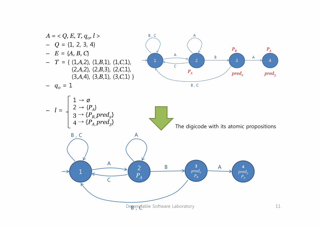
A = < Q E T q l >A = < Q, E, T, q0, l >– Q = {1, 2, 3, 4}– E = {A, B, C}

T = { (1 A 2) (1 B 1) (1 C 1)

PB PA

– T = { (1,A,2), (1,B,1), (1,C,1),(2,A,2), (2,B,3), (2,C,1),(3,A,4), (3,B,1), (3,C,1) }

– q0 = 1

pred2PA pred3

q0 1

– l =

1 → ø 2 → {PA}

{P d }3 → {PB, pred2}4 → {PA, pred3}

AB , C

The digicode with its atomic propositions

A

12

PA

3pred2

PB

4pred3

PA

ABA

C

B , CDependable Software Laboratory 11

• Formal definitions of automaton’s behavior– a path of automaton A :

– A sequence σ, finite or infinite, of transitions which follows each other– Ex.

– a length of a path σ :3 → 1 → 2 → 2 B A A

a length of a path σ :– | σ |– σ ‘s potentially infinite number of transitions: | σ | ∈ N ∪ {ω}

– a partial execution of A :– A path starting from the initial state q0

– Ex. – a complete execution of A :

– An execution which is maximal

1 → 2 → 2 → 3 A A B

– An execution which is maximal.– Infinite or deadlock

– a reachable state :– A state is said to be reachable,

– if a state appears in the execution tree of the automaton, in other words,– if there exists at least one execution in which it appears.


1 3 Printer Manager1.3 Printer ManagerPropositions

W = WaitingA printer shared by two users W = WaitingP = Printing nowR = Rest for now

0RARB

endA endB

A printer shared by two users

1 2 76 begA begB

reqA reqB

WARB

RAWB

RAPB

PARB

gA begB

reqAreqB

5P

4W

3W

endAendB

begAbegBPAWB

WAPB

WAWB

reqAreqB qAreqB


A = < Q, E, T, q0, l >– Q = {0, 1, 2, 3, 4, 5, 6, 7}

{ b b d d }– E = {reqA, reqB, begA, begB, endA, endB}– T = { (0,reqA,1), (0,reqB,2), (1,reqB,3), (1,begA,6), (2,reqA,3),

(2,begB,7), (3,begA,5), (3,begB,4), (4,endB,1), (5,endA,2), (6 end 0) (6 req 5) (7 end 0) (7 req 4) }(6,endA,0), (6,reqB,5), (7,endB,0), (7,reqA,4) }

– q0 = 0

0 → {RA, RB} , 1 → {WA, RB}

– l = 2 → {RA, WB} , 3 → {WA, WB}4 → {WA, PB} , 5 → {PA, WB}6 → {PA, RB} , 7 → {RA, PB}


• Properties of the printer manager to verify

1. We would undoubtedly wish to prove that any printing operation is 1. We would undoubtedly wish to prove that any printing operation is preceded by a print request.

• In any execution, any state in which PA holds is preceded by a state in which the proposition WA holds.

2. Similarly, we would like to check that any print request is ultimately satisfied. ( fairness property)

• In any execution, any state in which WA holds is followed by a state in which the proposition PA holds.

• Model checking techniques allow us to prove automatically that• Property 1 is TRUE, and• Property 2 is FALSE, for example 0 1 3 4 1 3 4 1 3 4 1 3 4 1 … (counterexample)


1 4 Few More Variables1.4 Few More Variables

I i f i l i l i bl• It is often convenient to let automata manipulate state variables.– Control : states + transitions– Data : variables (assumes finite number of values)

• An automaton interacts with variables in two ways:– Assignments– Guards


if ctr < 3Actr := ctr + 1 if ctr < 3 (guard)

B C (t iti l b l)

if ctr < 3B, Cctr := ctr + 1

ABA

B , C (transition label)

ctr := ctr + 1 (assignment)

1 2 3 4AB

ctr := 0

if ctr < 3C

1if ctr = 3

ctr := ctr + 1 A, Cctr := ctr + 1

if ctr = 3B, Cctr := ctr + 1if ctr = 3

B C

err

B, Cctr := ctr + 1

The digicode with guarded transitions

No more than 3 mistakes !!!


• It is often necessary, in order to apply model checking methods, y pp y g• to unfold the behaviors of an automaton with variables • into a state graph • in which the possible transitions appear and the configurations are clear marked.

• Unfolded automaton = Transition systemUnfolded automaton Transition system• has global states• transitions are no longer guarded• no assignments on the transitions


A B A1ctr=0

2ctr=0

3ctr=0

4ctr=0

B,C B,C

ABA

A

C

ctr=0

1

ctr=0

2

ctr=0

3

ctr=0

4

B,C B,C

ABA

A

C

1ctr=1

2ctr=1

3ctr=1

4ctr=1

B C B C

ABA

A

C

1ctr=2

2ctr=2

3ctr=2

4ctr=2

Unfolding

B,C B,C

ABA

A

A C

1ctr=3

2ctr=3

3ctr=3

4ctr=3

B,C B,CA, C

errctr 4

The digicode with error counting

Dependable Software Laboratory

ctr=4(Unfolded automaton)

19

1 5 Synchronized Product1.5 Synchronized Product

R l lif f d f d l• Real-life programs or systems are often composed of modules or subsystems.

– Modules/Components (composition) Overall systemC t t t ( h i ti ) Gl b l t t– Component automata (synchronization) Global automaton

A t t f ll t• Automata for an overall system– Often has so many global states– Impossible to construct it directly (State explosion problem)

Two composition ways– Two composition ways• With synchronization• Without synchronization


• An example without synchronization– A system made up of three counters (modulo 2, 3, 4)– They do not interact with each other– Global automaton = Cartesian product of three independent automata

AC3

1 0 3 1 1 3 1 2 3

AC2

0,0,3 0,1,3 0,2,3

1,0,3 1,1,3 1,2,3

AC4

0,0,2 0,1,2 0,2,2

1,0,2 1,1,2 1,2,2

2*3*4 = 24 states3*3*3 - 1 = 26 transitions per a state

(I D )

0,0,1 0,1,1 0 2 1

1,0,1 1,1,1 1,2,1(Inc, Dec, -)

24 * 26 = 624 transitions

, ,

0 0 0

0,1,1

0 1 0

0,2,1

1,0,0 1,1,0 1,2,0


0,0,0 0,1,0 0,2,0

21

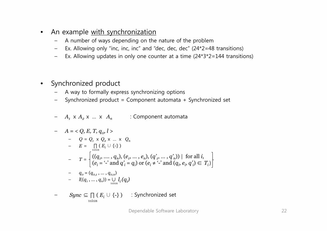
• An example with synchronization– A number of ways depending on the nature of the problem– Ex. Allowing only “inc, inc, inc” and “dec, dec, dec” (24*2=48 transitions)– Ex. Allowing updates in only one counter at a time (24*3*2=144 transitions)

• Synchronized product– A way to formally express synchronizing options – Synchronized product = Component automata + Synchronized set

A A A C t t t– A1 ⅹ A2 ⅹ … ⅹ An : Component automata

– A = < Q, E, T, q0, l >– Q = Q1 ⅹ Q2 ⅹ … ⅹ Qn1 2 n

– E =

– T =

∏ ( Ei∪ {-} )1≤i≤n

((q1, …. , qn), (e1, … , en), (q’1, … , q’n)) | for all i,(ei = ‘-’ and q’i = qi) or (ei ≠ ‘-’ and (qi, ei, q’i) ∈ Ti )

– q0 = (q0,1 , … , q0,n)– l((q1 , … , qn)) =

: Synchronized setSync ⊆ ∏ ( E ∪ { } )

∪ li (qi)1≤i≤n


– : Synchronized set 1≤i≤n

Sync ⊆ ∏ ( Ei∪ {-} )

22

• An example with synchronization– Ex. Allowing only “inc, inc, inc” and “dec, dec, dec” (24*2=48 transitions)

→ Strongly coupled version of modular counters– Sync = { (inc, inc, inc), (dec, dec, dec) }

– T = ((q1, …. , qn), (e1, … , en), (q’1, … , q’n)) | (e1, … , en) ∈ Sync(ei = ‘-’ and q’i = qi) or (ei ≠ ‘-’ and (qi, ei, q’i) ∈ Ti )

1,0,3 1,1,3 1,2,3

12 states0,0,2 0,1,2 0,2,2

1,0,1 1,1,1 1,2,1

12 states

24 transitions(inc, inc, inc) (dec, dec, dec)

Acoupl

Dependable Software Laboratory0,0,0 0,1,1 0,2,0

Accccoupl

23

• Reachable states– Reachability depends on the synchronization constraints

1,2,3 0,1,2 1,0,1 0,2,0 1,1,3 0,0,2

dec

inc

dec

inc

dec

inc

dec

inc

dec

inc

0,0,0 1,1,1 0,2,2 1,0,3 0,1,0 1,2,1dec

inc

dec

inc

dec

inc

dec

inc

dec

incdec inc decinc

dec

Accccoupl

Rearranged automaton → modulo 12 counter

• Reachability graphObt i d b d l ti h bl t t– Obtained by deleting non-reachable states

– Many tools to construct R.G. of synchronized product of automata– Reachability is a difficult problem

– State explosion problem


p p

24

1 6 Synchronization with Message Passing1.6 Synchronization with Message Passing

M i f k• Message passing framework– A special case of synchronized product– !m : Emitting a message

?m : Reception of the message– ?m : Reception of the message

– Only the transition in which !m and ?m pairs are executed simultaneously is permitted.

– Synchronous communication• Control/command system

A h i i– Asynchronous communication• Communication protocol (using channel/buffer)


• Smallish elevator– Synchronous communication (message passing)– One cabin– Three doors (one per floor)

One controller– One controller– No request from the three floors

The controller

?down ?upThe cabin

!close_2

!open_2free2 on2

2->0

!down

0 1 2?down ?down

?up?up

!close_1

!up !down!down

?close_i ?open_i !open_1free1 on1

!up !down!up

C O?open_i

?close_i

!close_0

free0 on0

0->2

!up !down

!up

Dependable Software LaboratoryThe ith door

!open_0free0 on0 !up

26

A t t f th lli h l t l• An automaton for the smallish elevator example– Obtained as the synchronized product of the five automata

– (door 0 door 1 door 2 cabin controller)– (door 0, door 1, door 2, cabin, controller)– Sync = { (?open_0, -, -, -, !open_0), (?close_0, -, -, -, !close_0),

(-, ?open_1, -, -, !open_1), (-, ?close_1, -, -, !close_1),(-, -, ?open_2, -, !open_2), (-, -, ?close_2, -, !clsoe_2),

d d(-, -, -, ?down, !down), (-, -, -, ?up, !up) }

P ti t h k• Properties to check• (P1) The door on a given floor cannot open while the cabin is on a different floor.• (P2) The cabin cannot move while one of the door is open.

• Model checkerC b ild th h i d d t f th 5 t t• Can build the synchronized product of the 5 automata.

• Can check automatically whether properties hold or not.


1 7 Synchronization by Shared Variables1.7 Synchronization by Shared Variables

A h h i i h h h• Another way to have components communicate with each other• Share a certain number of variables• Allow variables to be shared by several automatay

• Ex. The printer manager in Chapter 1.3– Problem: fairness property is not satisfiedProblem: fairness property is not satisfied


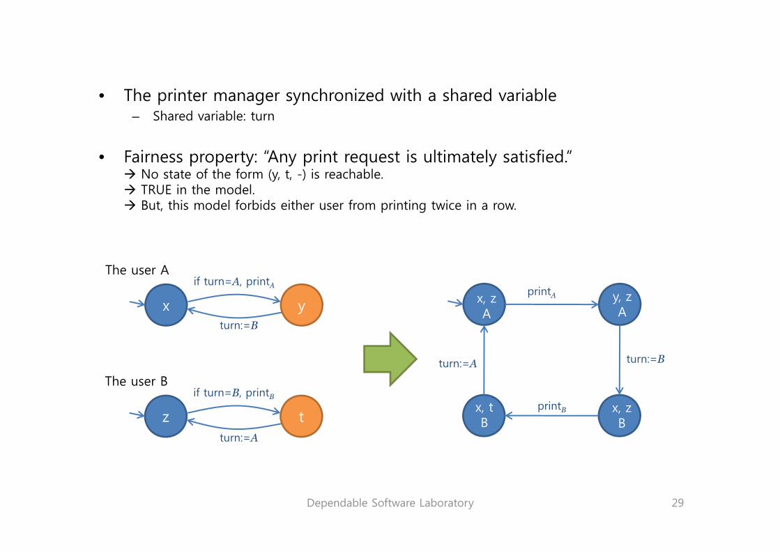
• The printer manager synchronized with a shared variable– Shared variable: turn

F i “A i i l i l i fi d”• Fairness property: “Any print request is ultimately satisfied.” No state of the form (y, t, -) is reachable. TRUE in the model. But, this model forbids either user from printing twice in a row.

The user A

x y

if turn=A, printA

turn:=B

printAx, zA

y, zA

The user Bif turn=B, printB

turn:=Bturn:=A

z tturn:=A

printBx, tB

x, zB


• Printer manager : A complete version with 3 variables [by Peterson]

– rA : a request from user A– rB : a request from user BrB : a request from user B– turn : to settle conflicts– Satisfies all our properties

1 2rA := true

The user A

1 2rB := true

The user B

1 2

turn:=Bif t A i t

rA := false

1 2

turn:=Aif t B i t

rB := false

4 3

if turn = A, printA

if rB = false printA

4 3

if turn = B, printB

if rA = false printBif rB false, printA if rA false, printB

A = < Q, E, T, q0, l >– Q = A ⅹ B ⅹ rA ⅹ rB ⅹ turn

AⅹB


4 ⅹ 4 ⅹ 2 ⅹ 2 ⅹ 2 = 128 states (only 128 reachable states)

30


Chapter 2. Temporal Logic

2 Temporal Logic2. Temporal Logic

M i i• Motivation:– The elevator example includes two properties

• “Any elevator request must ultimately be satisfied”• “The elevator never traverses a floor for which a request is pending without satisfying this request”The elevator never traverses a floor for which a request is pending without satisfying this request

– Dynamic behavior of the system

– In a first order logic,

• ∀t, ∀n ( app(n, t) ⇒ ∃t’ > t : serv(n, t’) )( app(n, t) ∧H(t’) ≠ n∧∃ttrav :

– But, the above notation(mathematics) is quite cumbersome.

pp , trav

• ∀t, ∀t’ > t, ∀n, t ≤ ttrav ≤ t’ ≤ H(ttrav) = n ) ⇒ (∃tserv : t ≤ tserv ≤ t’∧ serv(n, tserv) )

• Temporal Logic is a different formalism, better suited for our situation.


2 Temporal Logic2. Temporal Logic

T l L i• Temporal Logic– A form of logic specifically tailored for

• statements and reasoning• involving the notion of order in timeinvolving the notion of order in time

– Compared with the mathematical formulas• clearer and simpler• immediately ready for use (linguistic similarity of operators)• formal semantics (specification language tools)• formal semantics (specification language tools)

• Organization of Chapter 2– The Language of Temporal Logic– The Formal Syntax of Temporal Logic

Th S ti f T l L i– The Semantics of Temporal Logic– PLTL and CTL: Two Temporal Logics– The Expressivity of CTL*


2 1 The Language of Temporal Logic2.1 The Language of Temporal Logic

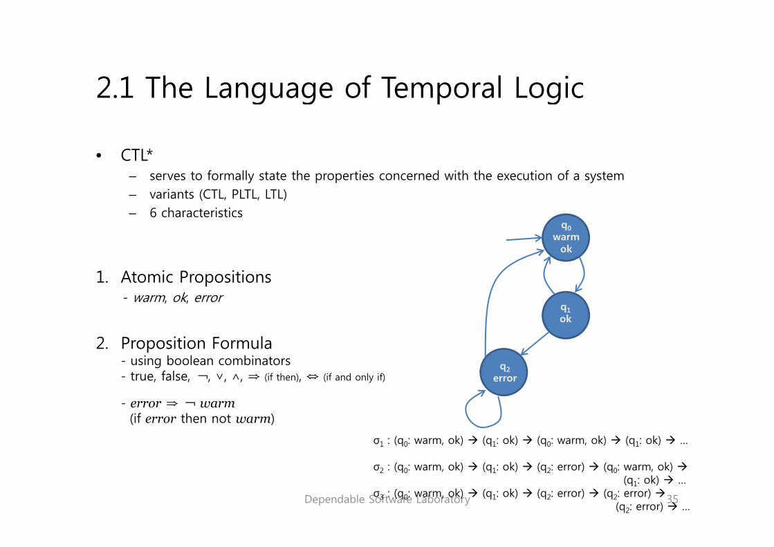
CTL*• CTL*– serves to formally state the properties concerned with the execution of a system– variants (CTL, PLTL, LTL)

6 characteristics– 6 characteristics

1 At i P iti

q0warm

ok

1. Atomic Propositions- warm, ok, error

q1ok

2. Proposition Formula- using boolean combinators- true, false, ￢, ∨, ∧, ⇒ (if then), ⇔ (if and only if)

q2error

- error ⇒ ￢ warm(if error then not warm)

σ1 : (q0: warm, ok) (q1: ok) (q0: warm, ok) (q1: ok) …


σ2 : (q0: warm, ok) (q1: ok) (q2: error) (q0: warm, ok) (q1: ok) …

σ3 : (q0: warm, ok) (q1: ok) (q2: error) (q2: error) (q2: error) …

35

3. Temporal combinatorsb t th i f t t l ti• about the sequencing of states along an execution

• X : next state• F : a future stateF : a future state• G : all the future states

• X P : the next state satisfies P• F P : a future state satisfies P without specifying which state

P will hold some day (at least once)• G P : all future states will satisfy P

P will always be P will always be

• alert ⇒ F halt : if we are currently in a state of alert, then we will later be ina halt state.

f f• G (alert ⇒ F halt ) : at any time, a state of alert will necessarily be followedby a halt state later.

• G (warm ⇒ F ￢warm ) : trueG (warm F warm ) : true• G (warm ⇒ X ￢warm ) : true

• G is the dual of F


• G ф ≡ ￢ F￢ф

36

4. Arbitrary nesting of temporal combinatorsy g p• giving temporal logic its power and strength

• GF ф : always there will some day be a state such that ф,ф i i fi d i fi i l f l h i id dф is satisfied infinitely often along the execution considered

• FG ф : all the time from a certain time onward, at each time instant, possibly excluding a finite number of instants

• GF warm ∨ FG error

5. U combinator• for until• ф1 U ф2 : ф1 is verified until ф2 is verified

ф2 will be verified some day, and ф1 will hold in the meantime

• G (alert ⇒ ( alarm U halt )) : starting from a state of alert, the alarm remains activateduntil the halt state is eventually and inexorably reacheduntil the halt state is eventually and inexorably reached.

• F ф ≡ true U ф• ф1 W ф2 ≡ (ф1 U ф2) ∨ G ф1 : weak until


6. Path quantifier• A ф : all the executions out of the current state satisfy property ф• E ф : from the current state, there exists an execution satisfying ф

• EF P : it is possible (by following a suitable execution) to have P some day• EG P : there exists an execution along which P always holds

• AF P : we will necessarily have P some day (regardless of the chosen execution)• AG P : always true

P PEF P : EG P :(= E￢ F￢P)

AF P :(= ￢ E￢FP)

AG P :(= ￢ EF ￢P)

P P P P

(= E￢ F￢P) (= ￢ E￢FP) (= ￢ EF ￢P)

P P P P P P P P


2 2 Formal Syntax of Temporal Logic2.2 Formal Syntax of Temporal Logic

Ab• Abstract grammar– needs parentheses, operator priority, specific set of atomic propositions, etc.– Most model checkers use a fragment of CTL* - CTL or LTL.

ф , Ψ : : = P1 | P2 | … (atomic proposition)| ￢ф | ф ∧Ψ | ф ⇒Ψ | (boolean combinators)| ф | ф ∧Ψ | ф ⇒Ψ | … (boolean combinators)| Xф | Fф | Gф | ф UΨ | … (temporal combinators)| Eф | Aф (path quantifiers)


2 3 The Semantics of Temporal Logic2.3 The Semantics of Temporal Logic

K i k• Kripke structure– Name of the models of temporal logic– Propositions labeling the states are important in CTL*

Transition labels (E) are neglected A < Q T q l > T ⊆ Q x Q– Transition labels (E) are neglected. A = < Q, T, q0 , l > , T ⊆ Q x Q

• SatisfactionA σ i ㅑф– A,σ,i ㅑф

• “at time i of the execution σ, ф is true.” • where σ is an execution of A, which not required to start at the initial state• A is often omitted.

– σ,i ㅑф : ф is satisfied at time i of σ– σ,i ㅑф : ф is not satisfied at time i of σ

– A ㅑф iff σ,0 ㅑΦ for every execution of σ of A• “the automaton A satisfies ф”• A ㅑ ф ≠ A ㅑ¬ф• σ i ㅑф = σ i ㅑ¬ф


• σ,i ㅑф = σ,i ㅑ¬ф

40

Semantics of CTL*

CTL*- Time is discrete.- Nothing exists between i and i + 1.

The instants are the points along the executions


- The instants are the points along the executions

41

2 4 PLTL and CTL: Two Temporal Logics2.4 PLTL and CTL: Two Temporal Logics

T l d l l i i d l h ki l• Two most commonly used temporal logics in model checking tools– PLTL (Propositional Linear Temporal Logic)– CTL (Computational Tree Logic)

fragments of CTL*– fragments of CTL*

• PLTLNo path quantifiers (A and E)– No path quantifiers (A and E)

– Linear time logic Path formula– For example, PLTL cannot distinguish A1 from A2

P,QA1 : P,QA2 :

Execution 1 : {P, Q} . {P}. {-}P

Q

P

Q

P{ , Q} { } { }

Execution 2 : {P, Q} . {P} . {Q}


Q Q

42

• CTL– Temporal combinators (X, F, U) should be under the immediate scope of path quantifier (A, E)– EX , AX , EU , AU , EF , EG , AG , AF , …– State formulas

– Truth only depends on the current state and the automaton regions made reachable by it– Truth only depends on the current state and the automaton regions made reachable by it– not depending on a current execution– q ㅑф : ф is satisfied in state q

C di i i h d– CTL can distinguish automata A1 and A2

P,QA1 : P,QA2 :

P P PA1,q0 ㅑ AX (EXQ∧ EX¬Q)A2,q’0 ㅑ AX (EXQ∧ EX¬Q)

Q Q

2,q 0 ㅑ ( Q Q)

– Potential reachability : AG EF P


y– Do not allow to express very rich properties along the paths.

43

Whi h t h CTL PLTL ?• Which to choose CTL or PLTL ?– To state some properties PLTL

– To perform exhaustive verification of a system CTL

b h– For both purposes CTL*

• Less popular• More complicated than PLTL

– CTL + Fairness properties FCTL

If e se model checking tools then e ha e no choice– If we use model checking tools, then we have no choice– SMV : CTL (CTL*)– SPIN : PLTL– VIS : CTL / PLTL


2 5 The Expressivity of CTL*2.5 The Expressivity of CTL

N l i hi k i b h d li• No logic can express anything not taken into account by the modeling decision made

• CTL* is rather expressive enough, when– Properties concern the execution tree of our automata

– CTL* combinators are sufficiently expressive– CTL* is almost always sufficient



Chapter 3. Model Checking

3 Model Checking3. Model Checking

M i i• Motivation:– Describe the principles underlying the algorithms used for model checking

The algorithm– The algorithm• Can find out whether a given automaton satisfies a given temporal formula• Different algorithms for CTL and PLTL

• Organization of Chapter 3– Model Checking CTL– Model Checking CTL– Model Checking PLTL– The State Explosion Problem


3 1 Model Checking CTL3.1 Model Checking CTL• Model checking algorithm for CTL

Developed in 1980s– Developed in 1980s– Runs in time linear in each of its components (automaton and CTL formula)– Relies on the fact that CTL can only express state formulas

• Basic principles– procedure marking

• Starting from a CTL formula ф• Mark for each state q of the automaton and for each sub-formula ψ of ф,q ψ ф,• Whether ψ is satisfied in state q

• Correctness of the algorithm– …– Hence, the marking of q is correct.

• Complexity of the algorithmComplexity of the algorithm– Model checking “ does A,q0ㅑΦ ? ” for a CTL formula ф– can be solved in time O( |A| ⅹ |ф| )

• O(|A|) : for marking the automaton• O(|ф|) : for each sub-formula in ф


• O(|ф|) : for each sub formula in ф– Linear!!!

49


3 2 Model Checking PLTL3.2 Model Checking PLTL

M d l h ki l i h f PLTL• Model checking algorithm for PLTL– Developed in 1980s, but too technical to cover in this course

PLTL uses path formulas– PLTL uses path formulas– No longer possible to rely on marking the automaton states

– A finite automaton will generally give rise to infinitely many different executions, g y g y y ,themselves often infinite in length

– Hence, PLTL uses a language theory : ω-regular expressionA t i f l i• An extension of a regular expression

• “*” : an arbitrary but finite number of repetitions– (a b* + c)*

• “ω”: an infinite number of repetitions


• Basic principleM d l h ki “ d Aㅑф ? ” f PLTL f l ф– Model checking “ does Aㅑф ? ” for a PLTL formula ф

– Reduces to a “ Are all the execution of A described by εф ? “

– A PLTL model checker construct an automaton B ф (recognizing executions which do notA PLTL model checker construct an automaton B¬ф (recognizing executions which do not satisfy ф )

– Strongly synchronize A and B¬ф A ⊙B¬фⅹ

– Finally reduces to “ Is the language recognized by A ⊙B¬ф empty ?”ⅹ

• A simple example– ф : G(P ⇒ XF Q) any occurrence of P must be followed (later) by an occurrence of Q– B¬ф there exists an occurrence of P after which we will never again encounter Q

P, Qu :

P, ¬Q¬P, ¬Qu2 :

q0

P, QP, ¬Qu :

q1

P, ¬Qu1 :

If it infinitely often stays in q1, then is B¬ф satisfied.


¬P, Q¬P, ¬Q

u0 : y y q1, ¬ф

52

P Q

ф : G(P ⇒ XF Q)

q0 q1

P, QP, ¬Qu1 :

P, ¬Q¬P, ¬Qu2 :

B¬ф :P, Q

P, ¬Q¬P, Q

¬P, ¬Q

u0 :

If it infinitely often stays in q1, then is B¬ф satisfied.

¬PP¬Q

t1 t5

“ does Aㅑф ? ”

A : ¬P¬Q

PQ

t4

¬P

t2 t3


¬P¬Q

53

A B¬ф : ⅹ⊙A B¬ф :

P

¬P¬Q

ⅹ⊙t5 u1

ⅹ⊙

¬P¬Q

t1 u0ⅹ⊙t5 u0

ⅹ⊙

¬P P

t1 u2

⊙t

¬P¬Q

PQ

ⅹ⊙t4 u0

P¬Q

PQ

ⅹ⊙t2 u2

ⅹ⊙t4 u2

ⅹ⊙t3 u2

ⅹ⊙t2 u0 ⅹ⊙t3 u0

¬P¬Q

⊙3 2

¬P¬Q

There are behaviors of A accepted by A B¬фⅹ⊙

The language recognized by is nonemptyA B¬фⅹ⊙


g g g y p y¬ф

Aㅑф54

• Construction of B ф• Construction of B¬ф– Very difficult technically– Automaton B¬ф must in general be able to recognize infinite words Büchi automata

• Complexity of the algorithm– B¬ф has size O(2|ф|) in the worst case– has size O(|A| ⅹ |B¬ф |)– If fits in computer memory, we can determine it in time O(|A| ⅹ |B¬ф |)

A B¬фⅹ⊙

A B¬фⅹ⊙

– Model checking “does A, q0ㅑф ?“ for a PLTL formula ф can be done in time O(|A| ⅹ 2|ф|)

• Reachability analysis – We can say that B¬ф observes the behavior of A when the two automata are synchronized.y ¬ф y– Observable automata = formal specification of the desired property

• UPPAAL• SPIN


3 3 The State Explosion Problem3.3 The State Explosion Problem

S l i bl• State explosion problem– The main obstacle encountered by model checking algorithms– Indeed, the algorithms rely on explicit construction of the automaton A

• Traversal and marking (in case of CTL)• Traversal and marking (in case of CTL)• Synchronization with B¬ф and seeking of reachable states and loops (in case of PLTL)

– In practice, the number of states of A is quickly very large

– If we use values that are not priori bounded (integers, a waiting queue, etc.), we cannot even apply it

– Explicit model checking Symbolic model checking (Chapter 4)



Chapter 4. Symbolic Model Checking

4 Symbolic Model Checking4. Symbolic Model Checking

S b li d l h ki• Symbolic model checking– Any model checking method attempting to represent symbolically states and transitions– A particular symbolic method in which BDDs are used to represent the state variables

• BDD : Binary Decision Diagram• BDD : Binary Decision Diagram

• Motivation:– State explosion is the main problem for CTL or PLTL model checkingp p g– State explosion occurs whenever we represent explicitly all states of automaton we use

– Represent very large sets of states concisely, as if they were in bulk.

• Organization of chapter 4– Symbolic Computation of State Sets– Binary Decision Diagrams (BDD)– Representing Automata by BDDs– BDD-based Model Checking


4 1 Symbolic Computation of State Sets4.1 Symbolic Computation of State Sets

I i i f S (ф)• Iterative computation of Sat(ф)– A = <Q, T, … >– Pre(S) : immediate predecessors of the states belonging to S in Q

Sat(ф) : set of states of A which satisfy ф– Sat(ф) : set of states of A which satisfy ф– ψ is the sub-formulas of ф

– Sat(¬ψ) = Q \ Sat(ψ) /* ==== Computation of Pre*(S) ==== */( ψ) Q \ (ψ)– Sat(ψ∧ψ’) = Sat(ψ) ∩ Sat(ψ’)– Sat(EX ψ) = Pre(Sat(ψ))– Sat(AX ψ) = Q \ Pre(Q \ Sat(ψ))

/ p ( ) /X := S;Y := { };while (Y != X) {

Y := X;X := X ∨ Pre(X);– Sat(EF ψ) = Pre*(Sat(ψ))

– … (others are defined in a similar way)

X := X ∨ Pre(X);}return X;

– The algorithms in Section 3.1 is an particular implementation of Sat(ф)

– Hence, Sat(ф) is an explicit representation of the state sets(ф) p p


• Which symbolic representations to use ?W h t th f ll i i iti– We have to access the following primitives:

1. A symbolic representation of Sat(P) for each proposition P ∈ Prop,2. An algorithm to compute a symbolic representation of Pre(S) from a symbolic

representation of S,p3. Algorithms to compute the complement, the union, and the intersection of the

symbolic representations of the sets,4. An algorithm to tell whether two symbolic representations represent the same set.

• Which logic for symbolic model checking?Logics based on state formulas– Logics based on state formulas

– CTL is the best. – Mu-calculus on tree is possible.

• Systems with infinitely many states– Symbolic approach naturally extends to infinite systems.y pp y y– New difficulties:

1. Much trickier to come up with symbolic representations2. Iterative computation Sat(ф) is no longer guaranteed to terminate.


4 2 Binary Decision Diagram (BDD)4.2 Binary Decision Diagram (BDD)

BDD• BDD– A particular data structure very commonly used for representing states sets symbolically– Proposed in 1980s ~ early in 1990s

– Make possible the verification of the system which cannot represent explicitly.

– Advantages:g1. Efficiency2. Simplicity3. Easy Adaptation4. Generality


• BDD structure

– Example• Consider n boolean variables x1, x2, … , xn associated with a tuple < b1, b2, … , bn >

• Suppose n = 4,• The set S of our interest is the set such that (b1∨ b3)∧ (b2⇒ b4) is true.• We have several ways to represent the set:• We have several ways to represent the set:

• S = {<F,F,T,F>, <F,F,T,T> , … >• S = (b1∨ b2)∧ (b3⇒ b4) • S = (b1∧ ¬b2)∨ (b1∧ b4)∨ (b3∧ ¬b2)∨ (b3∧ b4) DNF• …• Decision Tree Our choice.

b1?

n1

F T

b2?

n2

n4 n5

b2?

n3

n6 n7

F

F

T

TT F

b3? b3?

b4?b4?b4?b4?

n8 n9 n10 n11

b3? b3?

b4?b4?b4?b4?

n12 n13 n14 n15F TTTT FF F

Dependable Software LaboratoryF F T T F F F T T T T T F T F T

F F F F F F F FT T T TT T T T

63

• Decision tree reduction– A BDD is a reduced decision tree.– Reduction rules:

1. Identical sub-trees are identified and shared. (n8 and n10) l d di d li h (d ) leads to a directed acyclic graph (dag)

2. Superfluous internal nodes are deleted. (n7)

– Advantages:Advantages:1. Space saving2. Canonicity

n2 n3

b1?

n1

F T

b2? b2?

b1?

F T

b2?

b3? b3?

n4 n5

b2?

b3? b3?

n6 n7F T

TTTT

T F

FF F

Reduced

b2? b2?

b3? b3?

F

FT

T

TT

b4?b4?b4?b4?

n8 n9 n10 n11

b4?b4?b4?b4?

n12 n13 n14 n15F

F F F F F F F FT T T TT T T T

TTTT FF F

b4?F F

F

T

T


F F T T F F F T T T T T F T F T F T

Decision tree BDD64

• Canonicity of BDDsy– BDDs canonically represent sets of boolean tuples. (fundamental property of BDDs)– If the order of the variable xi is fixed, then there exists a unique BDD for each set S.

– Properties of BDDs1. We can test the equivalence of two BDDs in constant time.2. We can tell whether a BDD represents the empty set simply by verifying whether it

is reduced to a unique leaf Fis reduced to a unique leaf F.

• Operations on BDDsOperations on BDDs– All boolean operations

1. Emptiness test2. Comparison3 Complementation3. Complementation4. Intersection5. Union and other binary boolean operations6. Projection and abstractions

C l i li d i f h i– Complexity : linear or quadratic (for each operation) the same state explosion problems still exist.


4 3 Representing Automata by BDDs4.3 Representing Automata by BDDs

B f l i BDD b li d l h ki d• Before applying BDDs to symbolic model checking, we need to restate– Representing the states by BDDs– Representing transitions by BDDs

• Representing the states by BDDsConsider an automaton A with

b12

F

– Consider an automaton A with• Q = {q0, … , q6} b1

1, b21, b3

1

• var digit:0..9 b12, b2

2, b32, b4

2

• var ready:bool b13

b1 b2 b3 b1 b2 b3 b4 b1

b22

b32 b3?

F

T

• < b11, b2

1, b31, b1

2, b22, b3

2, b42, b1

3 >• < F, T, T, T, F, F, F, F > = <q3, 8, F >

b4?F

TT

F b42

– Let’s represent Sat(ready⇒ (digit > 2))• States <q, k, b> such that if b = T and k > 2• ready⇒ (digit > 2) ≡ ¬ ready∨ (digit > 2)

TF

b13 T


F T

66

• Representing transitions by BDDs– The same idea is applied.– <q3, 8, F > → <q5, 0, F > : < F, T, T, T, F, F, F, F, T, F, T, F, F, F, F, F >q3, , q5, , , , , , , , , , , , , , , , ,

– For example,

if digit ≠ 0, ready := T

– (<q, k, b>, <q’, k’, b’>) q = q1, k ≠ 0, q’ = q2, k’ = k , b’ = T

q1 q2g , y

q q1, k ≠ 0, q q2, k k , b T

( ¬b11 ∧¬b2

1∧ b31 )

∧ ( b12∨b2

2∨b32∨b4

2 )∧ ( ¬b’ 11 ∧b’ 21∧ ¬b’ 31 )∧ ( ¬b 1 ∧b 1∧ ¬b 1 )∧ ( b’ 12⇔b1

2 ∧ b’ 22⇔b22 ∧ b’ 32⇔b3

2 ∧ b’ 42 ⇔ b42 )

∧b’ 13


4 4 BDD based Model Checking4.4 BDD-based Model Checking

• BDDs can serve as an instance of symbolic model checking schemey g– Provide compact representations for the sets of states in an automaton– Support the basic sets of operations– Computation of Pre(S) in section 4.1 is very simple

• Implementation– SMV (chapter 12)

– Efficiency of BDDs depends on• BT representing the transition relation T (as containing pairs of states)• Choice of ordering for the boolean variables

Very easy to explode exponentially– Very easy to explode exponentially

• Perspective– Widely used from early 1990s– Widely used from early 1990s– Current work on model checking

• Aiming at applying BDD technology to solve more verification problems (ex. program equivalence)• Aiming at extending the limits inherent to BDD-based model checking


– Widely used throughout the VLSI design industry

68


Chapter 5. Timed Automata

5 Timed Automata5. Timed Automata

• “Temporal”p– “Trigger the alarm action upon detecting a problem”

• “Real-Time”Real Time– “Trigger the alarm less than 5 seconds after detecting a problem”

• Timed Automata• Timed Automata– Proposed by Alur and Dill in 1994.– An answer to this “real-time” needs

• Organization of chapter 5– Description of a Timed AutomataDescription of a Timed Automata– Networks of Timed Automata and Synchronization– Variants and Extensions of the Basic Model– Timed Temporal Logic


– Timed Model Checking

71

5 1 Description of Timed Automata5.1 Description of Timed Automata

T f d t l l t f ti d t t• Two fundamental elements of timed automata1. A finite automaton (assumed instantaneous between states)2. Clocks

• An examplepc ≥ 5, ?msg, c := 0

init verify alarm- , ?msg, c := 0 c < 5 , ?msg, -


• Clocks and transitions– Clocks

• Variables having non-negative real values in R• All clocks are null in the initial system states• All clocks evolve at the same speed synchronously with time• All clocks evolve at the same speed, synchronously with time

– Transitions• Three items

d• A guard• An action (label)• Reset of some clocks

– The system operates as if equipped with• A global clock• Many individual clocks (each is synchronized with the global clock)


• Configurations and executions– Configuration of the systemConfiguration of the system

• (q, v)• q : a current control state of the automaton• v : the value of each clock

• We also refer to v as a valuation of the automaton clocks.• Timed automata does not fix the time unit under consideration

E ti f th t– Execution of the system• (usually infinite) sequence of configurations • A mapping ρ from R to the set of configuration

• Configurations change in two ways– Delay transition– Discrete transition (or action transition)

(init, 0) → (init, 10.2) → (verify, 0) → (verify, 5.8) → (verify, 0) → (verify, 3.1) → (alarm, 3.1) → …?msg ?msg ?msg

Delay transition

Discrete transition

• Trajectory– ρ(0) : the initial state


ρ( )– ρ(12.3) = (verify, 2.1)

74

5 2 Networks of Timed Automata and Synchronization5.2 Networks of Timed Automata and Synchronization

I i f l b ild i d d l i i f hi• It is useful to build a timed model in a composite fashion, – by combining several parallel automata synchronized with one another a timed automata network

• Executions of a timed automata network– All automata components run in parallel at the same speed– Their clocks are all synchronized to the same global clockTheir clocks are all synchronized to the same global clock

– (q , v) : a network configuration• q : a control state vector

f• v : a function associating each network clock with its value at the current time

• SynchronizationTi d t t h i t iti ( ll ) b tti th l k– Timed automata synchronize on transitions (as usually) by resetting the clocks

– The clocks which were not reset are unchanged– No concurrent write conflicts on clocks, since reset writes a zero value and nothing else


App ExitApp Exit

far near on far

AppExit

far near

AppCt := 0 up lower

AppCb := 0

App

on

2 < Ct < 5Ct := 0

1 < Ct < 2Exit

raise down

Cb := 0Exit

Cb := 01 < Cb < 2 1 < Cb < 2

raise

AppExit

ExitCb := 0Train Gate


• Example : modeling a railroad crossing

76

5.3 Variants and Extensions of the Basic Models

• Many variants, and three extensions

1. Invariants– Liveness hypothesis in the untimed model– Invariant: a state’s condition on the clock values which must always hold in the stateInvariant: a state s condition on the clock values, which must always hold in the state– Example: near (invariant: Ht < 5), on (invariant: Ht < 2), lower/raise (invariant: Hb < 2)

2. Urgency– Used when cannot tolerate a time delay

Represented in the system configurations not in the transitions

x < 2c1

y < 2c2

– Represented in the system configurations, not in the transitions– Allowing urgent/synchronized behaviors in a more natural way

c3c3

3. Hybrid linear system– Models dynamic variables (in a form of differential equations)

H T h– HyTech


5 4 Timed Temporal Logic5.4 Timed Temporal Logic

Gi d ib d k f i d• Given a system described as a network of timed automata,• We wish to be able to state/verify properties of this system

– Temporal properties• “When the train is inside the crossing, the gate is always closed.”

– Real-time properties• “The train always triggers an Exit signal within 7 minutes of having emitted an App signal.”

• Three ways to formally state real-time properties1. Express it in terms of the reachability of some sets of configurations

2. Use observer automata in PLTL model checking• Given a property ф , a network R• Testing reachability of some states in the product R || Aф

• UPPAAL , HYTECHU , C

3. Use a timed logic• TCTL (Timed CTL)

Et• Etc.


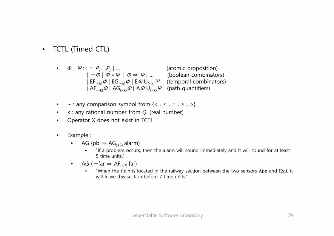
• TCTL (Timed CTL)

• Φ , Ψ : : = P1 | P2 | … (atomic proposition)| ￢Φ | Φ ∧Ψ | Φ ⇒ Ψ | … (boolean combinators)| EF(~k)Φ | EG(~k)Φ | EΦ U(~k)Ψ (temporal combinators)| AF(~k)Φ | AG(~k)Φ | AΦ U(~k)Ψ (path quantifiers)| ( k) | ( k) | ( k) p q

• ~ : any comparison symbol from {< , ≤ , = , ≥ , >}• k : any rational number from Q. (real number)

d i i• Operator X does not exist in TCTL

• Example :• AG (pb ⇒ AG(≤5) alarm)AG (pb AG(≤5) alarm)

• “If a problem occurs, then the alarm will sound immediately and it will sound for at least 5 time units.”

• AG (￢far ⇒ AF(<7) far)• “When the train is located in the railway section between the two sensors App and Exit itWhen the train is located in the railway section between the two sensors App and Exit, it

will leave this section before 7 time units.”


5 5 Timed Model Checking5.5 Timed Model Checking

Wi h i d d TCTL l i• With timed automata and TCTL logic• We wish to obtain a model checking algorithm for them.

• Difficulties : Automaton has an infinite number of configurations, since 1. Clock values are unbounded2. The set of real numbers used in clocks is dense

Overcome it with the equivalence classes, called “regions”

E l k ith k 0 1 2 x– Example: x1, x2 ~ k with k = 0, 1, 2• 28 regions

x2

r27

r4

(1)

r9r7


x1(1) (2)

r0r8 80

• Complexity

• Model checking algorithms are complicated• Model checking algorithms are complicated.• The number of regions grows exponentially.

• O(n!Mn)( )• n: number of clocks• M: upper bounds of every constant

• No general and efficient method is likely to exist ( vs linear complexity in CTL)• No general and efficient method is likely to exist. ( vs. linear complexity in CTL)• PSPACE-complete problem

• Existing tools focus on defining adequate data structures for handing sets of regionsg g q g g “zones”

• Existing tools have been successfully usedH T h- HyTech

- KRONOS- UPPAAL


Conclusion of Part IConclusion of Part I

M d l h ki i ifi i h i• Model checking is a verification technique

• It consists of three steps:p1. Representation of a program or a system by an automaton2. Representation of a property by a logical formula3. Model checking algorithm

• Model checking is a powerful but restricted tool:– Powerfulness: exhaustive and automatic verification

Li i i d l i b i– Limitation: due to complexity barriers– In practice, the size of system is indeed the main obstacle yet to overcome.

• Model checker users are forced to simplify the model under analysis, until it is manageable. (Abstraction)



Part II. Specifying with Temporal Logic


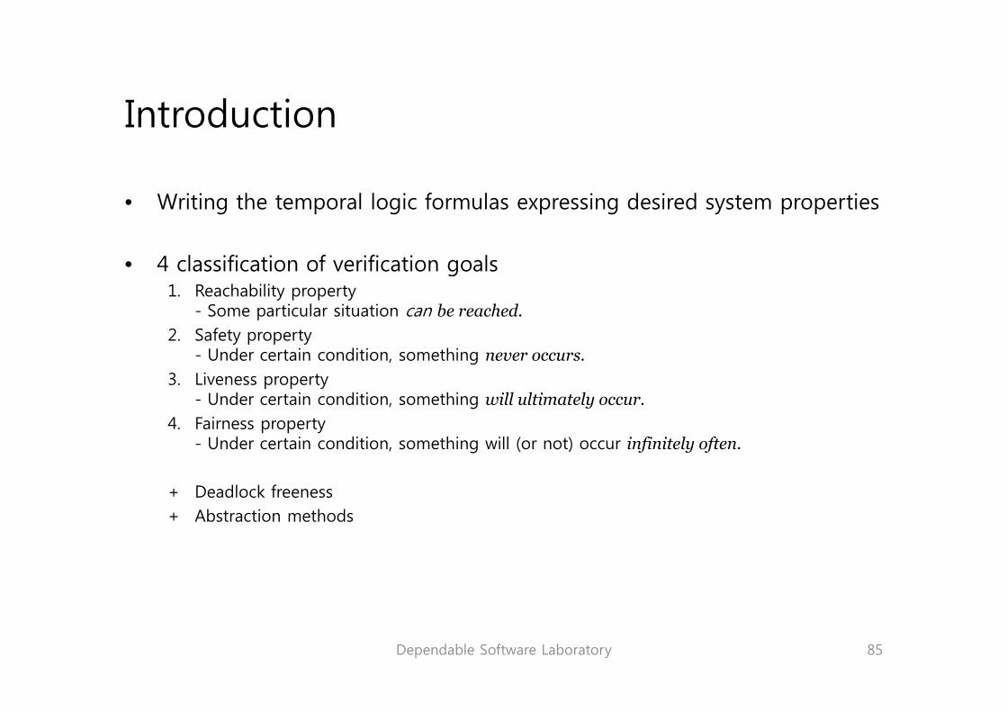
W i i h l l i f l i d i d i• Writing the temporal logic formulas expressing desired system properties

• 4 classification of verification goalsg1. Reachability property

- Some particular situation can be reached.2. Safety property

- Under certain condition something never occurs- Under certain condition, something never occurs.3. Liveness property

- Under certain condition, something will ultimately occur.4. Fairness property

d i di i hi ill i fi i l f- Under certain condition, something will (or not) occur infinitely often.

+ Deadlock freeness+ Abstraction methods+ Abstraction methods


Chapter 6. Reachability Properties

Chapter 6 Reachability PropertiesChapter 6. Reachability Properties

• Reachability propertyy p p y– Some particular situation can be reached.

– Examples:• (R1) “ We can obtain n<0 ”• (R2) “ We can enter a critical section ” simple• (R3) “ We cannot have n<0 “• (R4) “ We cannot reach the crash state “ negation of the simple• (R5) “ We can enter the critical section without traversing n=0 “ with conditional restricts• (R6) “ We can always return to the initial state “ stronger / nested• (R7) “ We can return to the initial state “

• Organization of Chapter 6R h bilit i T l L i– Reachability in Temporal Logic

– Model Checkers and Reachability– Computation of the Reachability Graph


6 1 Reachability in Temporal Logic6.1 Reachability in Temporal Logic

• EF Φ– “ There exists a path from the current state along which some state satisfying Φ “

– (R1) “ We can obtain n<0 ”• EF (n<0)• EF (n<0)

– (R2) “ We can enter a critical section ” • EF crit_sec

– (R3) “ We cannot have n<0 “• ¬EF (n<0)

– (R4) “ We cannot reach the crash state “ • ¬EF crash• AG ¬crash • “ Along every path, at any time, ¬crash ”

– (R5) “ We can enter the critical section without traversing n=0 “ • E (n≠0) U crit_sec• “ There exists a path along which n ≠ 0 holds until crit sec becomes true “• There exists a path along which n ≠ 0 holds until crit_sec becomes true.

– (R6) “ We can always return to the initial state “ • AG ( EF init )

– (R7) “ We can return to the initial state “


• EF init

88

6 2 Model Checkers and Reachability6.2 Model Checkers and Reachability

R h bili i i ll h i if• Reachability properties are typically the easiest to verify.• All model checkers can answer it in principle by simply examining their

reachability graph.

• But they do vary in richness.– conditional reachabilityy– nested reachability– etc.

• Design/CPN is specifically designed for reachability property verification.


6.3 Computation of the Reachability Graph

• The effective construction of set of reachable states are non-trivial.– Several automata are synchronized.y

• Algorithms dealing with reachability problems1 Forward chaining1. Forward chaining2. Backward chaining3. “On-the-fly” exploration

• Forward chaining– A natural approach– from initial states add their successors until saturation– Difficulty: potential explosion of the set constructed

• Backward chaining– from target states add immediate predecessors until saturation– then, test whether some initial states are in there (like pre*(S) in Section 4.1)– Drawback

1 Target states need to be fixed before


1. Target states need to be fixed before.2. Computing immediate predecessors is generally more complicated than that of successors.

90

“O th fl ” l ti• “On-the-fly” exploration– Explore the reachability graph without actually building it– Construction is performed partially, as the exploration proceeds, without remembering

everything already visited.everything already visited.

– Background assumption• Present-day computers are more limited in memory resources than in processing speed

– It is efficient mostly when1. Target set is indeed reachable. (“Yes” requires no exhaustive explorations)2. Can operate in forward or backward manners (The forward is the traditional)p ( )3. May apply to some systems with infinitely many states



Chapter 7. Safety Properties

7 Safety Properties7. Safety Properties

S f• Safety property– Under certain conditions, an (undesirable) event never occur.

Examples:– Examples:• (S1) “ Both processes will never be in their critical sections simultaneously (mutual exclusion) ”• (S2) “ Memory overflow will never occur ”• (S3) “ The situation … is impossible “

(S4) “ A l h k i i h i i i i i h ’ “ i h di i• (S4) “ As long as the key is not in the ignition position, the car won’t start “ with conditions

• ¬ safety property = reachability property• ¬ reachability property = safety property

• Organization of Chapter 7Safety Properties in Temporal Logic– Safety Properties in Temporal Logic

– A Formal Definition– Safety Properties in Practice– The history Variables Methody


7 1 Safety Properties in Temporal Logic7.1 Safety Properties in Temporal Logic

AG Φ• AG ㄱΦ– “ Φ never occurs. “

(S1) “ Both processes will never be in their critical sections simultaneously ”– (S1) Both processes will never be in their critical sections simultaneously • AG ¬(crit_sec1 ∧ crit_sec2)

– (S2) “ Memory overflow will never occur ”• AG ¬overflow

– (S3) “ The situation … is impossible “• AG ¬situation

– (S4) “ As long as the key is not in the ignition position, the car won’t start “ • A (¬start W key) (using weak until)A ( start W key) (using weak until)• A (¬start U key) Not a safety property !


7 2 A Formal Definition7.2 A Formal Definition

S i h i i• Syntactic characterization– Safety properties can be written in the form AG Φ¯

• Φ¯ is a past temporal formula

– When a safety property is violated it should be possible to instantly notice it– When a safety property is violated, it should be possible to instantly notice it.– We can only notice it, in the current state, relying on events which occurred earlier.

• Temporal logic with past– CTL* does not provide past combinators– But, we can use a mirror image of future combinators ( F-1, X-1 )


• AG Φ¯ in practice– (S1) AG ¬(crit sec1 ∧ crit sec2) ( ) ( _ 1 _ 2)

• ¬(crit_sec1 ∧ crit_sec2) is a ф¯

– (S4) A ¬start W key • Can be rewritten in the form: AG (start ⇒ F-1 key)• “ It is always true (AG) that if the car starts then (⇒) the key was inserted beforehand (F-1) “• It is always true (AG) that if the car starts, then (⇒) the key was inserted beforehand (F 1).

– If Ψ1 and ψ2 are safety properties, then Ψ1 ∧ ψ2 again a safety property.• But, Ψ1 ∨ ψ2 is in general not

• Safety properties and diagnostic– If AG Φ¯ is not satisfied, then there necessarily exists a finite path leading from init to it.

Since Φ¯ is a past form la– Since Φ is a past formula.


7.3 Safety Properties in Practice

• Safety properties are verified simply by submitting it to a model checker.• But, in real life, hurdles spring up.

• A simple case: non-reachability– The most safety properties– ¬EF (crit_in1 ∧ crit_in2) = AG Φ¯

• ¬(crit_in1 ∧ crit_in2) is a present formula

• Safety without pastSafety without past– A (¬start W key) is used more often than AG (start ⇒ F-1 key)– But, no model checker is able to deal with past formulas. So, mixed logics are used.– The problem is their identification. p If they are identified, then it can be dealt with similarly Otherwise, we have to use the method of history variables (in section 7.4)

• Safety with explicit pastSafety with explicit past– No model checker is able to handle temporal formula with past.– Two approaches:

1. Eliminate the past (in principle, it is possible to translate mixed formulas to pure-future ones)


– AG (ф⇒ F-1 ψ) ≡ A (¬фW ψ) , but not easy.2. History variable method (section 7.4)

98

7 4 The History Variables Method7.4 The History Variables Method

Ski d !!!• Skipped !!!



Chapter 8. Liveness Properties

8. Liveness Properties• Liveness property

– Under certain conditions, some event will ultimately occur. – Some happy event will occur in the end.

– Examples:• (L1) “ Any request will ultimately be satisfied ”(L1) Any request will ultimately be satisfied • (L2) “ By keeping on trying, one will eventually succeed ”• (L3) “ If we call on the elevator, it will bound to arrive eventually “• (L4) “ The light will turn green (some day regardless of the system behavior)“• (L5) “ After the rain the sunshine “• (L5) After the rain, the sunshine • (L6) “ The program will terminate “

– Two broad family of liveness properties1. Simple liveness : progress (Chapter 8)2. Repeated liveness : fairness (Chapter 10)

Organization of Chapter 8• Organization of Chapter 8– Simple Liveness in Temporal Logic– Are Liveness Properties Useful?– Liveness in the Model Liveness in the Properties


Liveness in the Model, Liveness in the Properties– Verification under Liveness Hypotheses– Bounded Liveness 102

8 1 Simple Liveness in Temporal Logic8.1 Simple Liveness in Temporal Logic

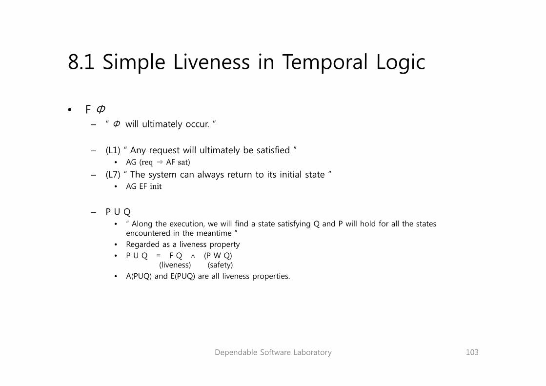
F Φ• F Φ– “ Φ will ultimately occur. “

(L1) “ Any request will ultimately be satisfied ”– (L1) Any request will ultimately be satisfied • AG (req ⇒ AF sat)

– (L7) “ The system can always return to its initial state ”• AG EF init

– P U Q• “ Along the execution, we will find a state satisfying Q and P will hold for all the states

encountered in the meantime “• Regarded as a liveness property• P U Q ≡ F Q ∧ (P W Q)

(liveness) (safety)• A(PUQ) and E(PUQ) are all liveness properties.


8 2 Are Liveness Properties Useful?8.2 Are Liveness Properties Useful?

Ab li i• Abstract liveness properties

– “ If we call on the elevator, it is bound to arrive eventually “• It yields no information from a utilitarian viewpoint• It yields no information, from a utilitarian viewpoint.• “Abstract” liveness property

– “ An event will occur within at most x time unit “I i f l b b f• It is useful, but became a safety property.

• “Bounded” liveness property

– But, it is still useful• “Abstract” more general than “concrete”• “Abstract” more efficient than “concrete”• “Abstract” and “concrete” are not contradictory


8 3 Liveness in the Model Liveness in the Properties8.3 Liveness in the Model, Liveness in the Properties

• Two different roles in the verification process1 Li ti i h t if1. Liveness properties : we wish to verify2. Liveness hypotheses : we make on the system model

• When we use a mathematical model( t t ) to represent a real system• When we use a mathematical model(automata) to represent a real system, – The semantics of the model in face define implicit safety and liveness hypotheses.– Safety hypothesis :

• Clear• It can flip from q to q’ only if it includes a transition going from q to q’.

– Liveness hypothesis :• Not clear• The system will chain transitions as long as possible (to a block state or accepting states)The system will chain transitions as long as possible. (to a block state or accepting states)• “ The system does not terminate without reason, or remain inactive indefinitely without reason. “• Can be subtle and cause errors :

In state x, will always end up wishing printing. Different from the real world’s behavior !!!


• One must be aware of the premises of the models used and check their adequacy !

105

8 4 Verification under Liveness Hypotheses8.4 Verification under Liveness Hypotheses

V if h ifi d l b h i i f i• Verify that specific model behaviors satisfy a given property :– фv : only the model which the liveness hypotheses hold– Ψ : a property

– Verify фv ⇒ ψ is sufficient!!!

– If ψ is a CTL propertyψ p p y• AF ( E PUQ ) A ( фv ⇒ FE (фv ∧ P U Q) )


8 5 Bounded Liveness8.5 Bounded Liveness

• Bounded liveness property– A liveness property that comes with a maximal delay which the desired situation must

occur.– Safety properties from a theoretical viewpoint.– Can be rewritten in a form AG (ψ ⇒ F-1 ψ )– Can be rewritten in a form AG (ψ2 ⇒ F ψ1)– Not as important as safety properties

• Bounded liveness in timed systems– Often used in the specification of timed systems (in Chapter 5)– Explicit constraints on delays TCTL !!!

– (BL1) “ The program terminates in less than ten seconds “• AF<10s end bounded liveness property• AG (¬end ⇒ F-1 start ) safety property• AG (¬end ⇒ F <10s start ) safety property

– (BL2) “ Any request is satisfied in less than five minutes “• AG ( req ⇒ AF<5m sat ) bounded liveness property

AG ( (F 1 G 1 ) f t t


• AG ( ¬(F-1=5mreq ∧ G-1

≤5m¬sat ) safety property

107


Chapter 9. Deadlock-freeness

9 Deadlock freeness9. Deadlock-freeness

D dl k f• Deadlock-freeness– A special property – “ The system can never be in a situation on which no progress is possible. “

– Correct property relevant for systems that are supposed to run indefinitely.– A set of properly identified final states will be required to be deadlock-free.

• Organization of Chapter 9• Organization of Chapter 9– Safety? Liveness?– Deadlock-freeness for a Given Automaton– Beware of Abstractions!`


9 1 Safety? Liveness?9.1 Safety? Liveness?

AG EX• AG EX true

– “ Whatever the state reached may be (AG), there will exist an immediate successor state (EX true) “(EX true)

– Not the form of AGф-1

– Deadlock-free is not a safety property.

– Can be verified if the model checker at our disposal can handle AG EX true.


9 2 Deadlock freeness for a Given Automaton9.2 Deadlock-freeness for a Given Automaton

W i hi k f d dl k f f• We sometimes think of deadlock-freeness as a safety property– For a given automaton, we can describe the deadlock states explicitly.– But, it is up to the automaton we obtain.

– For example,

if x > 0x := x + 1A

s1 s2x:=0, y:=0

x = x + 1

s3if x = y

AG EX true hold! (liveness property)

AG ¬(s3 ∧ x≤0) hold! (safety property)

A

y = y + 1

if x > 0

s1 s2x:=0, y:=0

x = x + 1

s3if x = y

if x > 0x := x + 1

AG EX true not hold! (liveness property)

AG ¬(s3 ∧ x≤0) hold! (safety property)

A’


y

112

9 3 Beware of Abstractions!9.3 Beware of Abstractions!

if x > 0x := x + 1

s1 s2x:=0, y:=0

x = x + 1

s3if x = y

x := x + 1A

Deadlock-free

y = y + 1

if > 0

Abstraction

s1 s2x:=0, y:=0

x = x + 1

s3if x = y

if x > 0x := x + 1A’

Deadlockif x = y

Abstraction

1 2 3

A’’

Deadlock-free


s1 s2 s3

113


Chapter 10. Fairness Properties

10 Fairness Properties10. Fairness Properties

F i P• Fairness Property– Under certain conditions, an event will occur (or will fail to occur) infinitely often

Examples:– Examples:• (F1) “ The gate will be raised infinitely often”• (F2) “ If access to a critical section is infinitely often requested, then access will be granted

infinitely often “

– repeated liveness or repeated reachability

• Organization of Chapter 10– Fairness in Temporal Logic– Fairness and NondeterminismFairness and Nondeterminism– Fairness Properties and Fairness Hypothesis– Strong Fairness and Weak Fairness– Fairness in the Model or in the Property?


10 1 Fairness in Temporal Logic10.1 Fairness in Temporal Logic

GF P• GF P

– “ We meet a state in which P holds infinitely often “There is no last state in which P holds– There is no last state in which P holds.

– Fairness properties cannot be expressed in pure CTL• (F1) “ The gate will be raised infinitely often” A ( GF gate_raised )

• (F2) “ If access to a critical section is infinitely often requested, then access will be granted infinitely often “ A ( GF crit_req ⇒ FG crit_in )

– FCTL or ECTL+

• CTL + fairness• O( |A| ⅹ |ф|2 )• Many tools (like SMV) considers the fairness hypotheses as part of model than choosing FCTL


10 2 Fairness and Nondeterminism10.2 Fairness and Nondeterminism

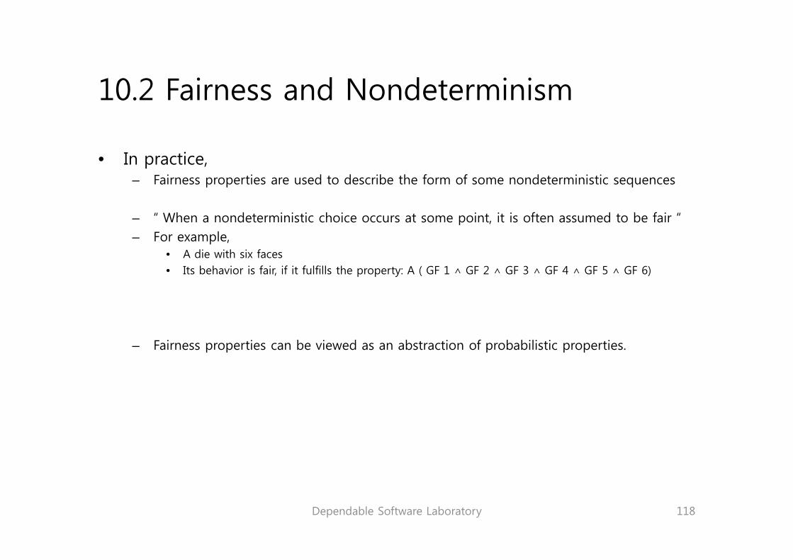
I i• In practice, – Fairness properties are used to describe the form of some nondeterministic sequences

“ When a nondeterministic choice occurs at some point it is often assumed to be fair “– When a nondeterministic choice occurs at some point, it is often assumed to be fair – For example,

• A die with six faces• Its behavior is fair, if it fulfills the property: A ( GF 1 ∧ GF 2 ∧ GF 3 ∧ GF 4 ∧ GF 5 ∧ GF 6)

Fairness properties can be viewed as an abstraction of probabilistic properties– Fairness properties can be viewed as an abstraction of probabilistic properties.


10 3 Fairness Properties and Fairness Hypotheses10.3 Fairness Properties and Fairness Hypotheses• Fairness properties are very often used as hypotheses.

• An example:– Classical alternating bit protocol

• A : a transmitter• A : a transmitter• B : a receiver• AB : a line for messages• BA : a line for message acknowledgements

M b l t d t i i ti b h i f AB d BA• Messages can be lost non-deterministic behavior of AB and BA

– Liveness property : “ Any emitted message is eventually received “• G ( emitted ⇒ F received )• Fail !!!• The model allows to systematically lose all messages.• Our original intension : “unreliable” line, not the whole lose Fairness hypothesis !!!• A ( GF ¬loss ⇒ G ( emitted ⇒ F received ) )

ffairness hypothesis liveness property

– Repeated liveness property : “ If infinitely many messages are emitted, then infinitely many messages will be transmitted “

repeated liveness property


repeated liveness property

• A ( GF ¬loss ⇒ ( GF emitted ⇒ GF received ) )fairness hypothesis repeated liveness hypothesis

119

10 4 Strong Fairness and Weak Fairness10.4 Strong Fairness and Weak Fairness

F i• Fairness property– “ If P is continually requested, then P will be granted (infinitely often) “

W k f i• Weak fairness– Assume that P is requested without interruption– ( FG request_P ) ⇒ F P

( FG request P ) ⇒ GF P– ( FG request_P ) ⇒ GF P

• Strong fairness– Assume that P is requested in an infinitely repeated manner possibly with interruptions– Assume that P is requested in an infinitely repeated manner, possibly with interruptions– ( GF request_P ) ⇒ F P– ( GF request_P ) ⇒ GF P

• No difference when using them for model checking of finite systems


10 5 Fairness in the Model or in the Property?10.5 Fairness in the Model or in the Property?

Th b i• The best way is– Model = automaton + fairness hypotheses– Since the second can change independently from the first

like SMV model checker– like SMV model checker



Chapter 11. Abstraction Methods

11 Abstraction Methods11. Abstraction Methods

Ab i M h d• Abstraction Methods– A family of techniques used to simplify automata– Simplification aiming at verifying a system (faster) using a model checking approach

– Examples:• (Pb1) “ Does Aㅑф ? ” a complex problem• (Pb2) “ Does A’ㅑф’ ? ” a much simpler problem

– “ tricks of the trade “

O i ti f Ch t 11• Organization of Chapter 11– When Is Model Abstraction Required? – Abstraction by State Merging

What Can Be Proved in the Abstract Automaton?– What Can Be Proved in the Abstract Automaton?– Abstraction on the Variables– Abstraction by Restriction– Observer Automata


11 1 When Is Model Abstraction Required?11.1 When Is Model Abstraction Required?

T i f i i f d l b i• Two main types of situations for model abstraction1. Size of the automaton

• Too large : • Too many variablesToo many variables• Too many automata in parallel• Too many clocks in the timed automata

2. Type of the automaton• Other types of automata• Other types of automata• Using integer variables, communication channels, clocks, priorities, etc.

• Three classical abstraction methods1. Abstraction by State Merging2. Abstraction on the Variables3 Ab t ti b R t i ti3. Abstraction by Restriction


11 2 Abstraction by State Merging11.2 Abstraction by State Merging

F ldi• Folding

– Viewing some states of an automaton as identicalThe most important question : Correctness!– The most important question : Correctness!

– For example,• The digicode door lock with error counters (in Chapter 1)• Focusing on the error counter.

• Correctness problem: – All states in A’ can be reached through the letter A, but not in Ag


A B A1ctr=0

2ctr=0

3ctr=0

4ctr=0

A, B…

B,C B,C

ABA

A

C

ctr=0

1

ctr=0

2

ctr=0

3

ctr=0

4

A

ctr=0

A, B

A, B, C

B,C B,C

ABA

A

C

ctr=1

1

ctr=1

2

ctr=1

3

ctr=1

4

A A’A

A

…ctr=1

4…

A B

A, B, C

B,C B,C

ABA

A

C

1ctr=2

1

2ctr=2

2

3ctr=2

3

4ctr=2

4 A, B

A

A

…ctr=2

A, B

A, B, C

B,C B,C

BA

A, C

1ctr=3

2ctr=3

3ctr=3

4ctr=3

A, B

A, B, C

…ctr=3

errerr

ctr=4

errctr=4


11 3 What Can be Proved in the Abstract Automaton?11.3 What Can be Proved in the Abstract Automaton?

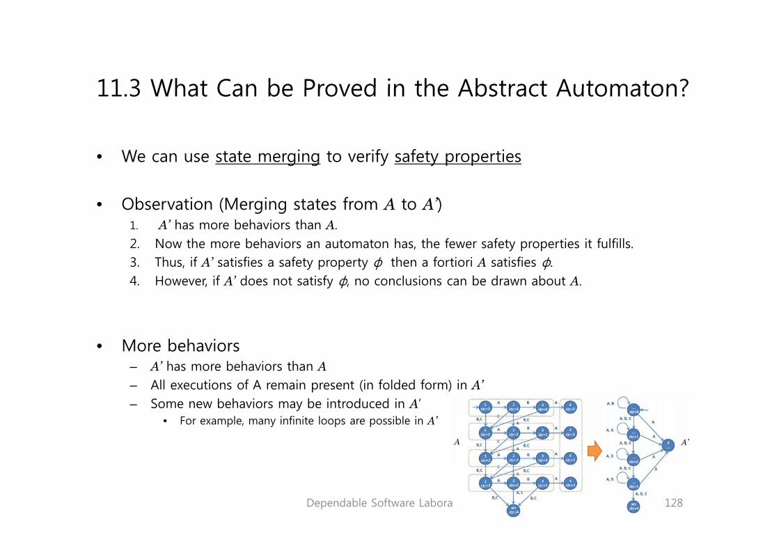
W i if f i• We can use state merging to verify safety properties

• Observation (Merging states from A to A’)g g1. A’ has more behaviors than A.2. Now the more behaviors an automaton has, the fewer safety properties it fulfills.3. Thus, if A’ satisfies a safety property ф then a fortiori A satisfies ф.

f d f l b d b4. However, if A’ does not satisfy ф, no conclusions can be drawn about A.

• More behaviors– A’ has more behaviors than A– All executions of A remain present (in folded form) in A’

S b h i b i t d d i A’– Some new behaviors may be introduced in A’• For example, many infinite loops are possible in A’


• Preserving safety properties– Necessary to ensure that the property ф is indeed a safety propertyNecessary to ensure that the property ф is indeed a safety property.

• One-way preservation– If A’ does not satisfies ф , then A’ satisfies￢фIf A does not satisfies ф , then A satisfies ф .– But, in general the negation of a safety property is not a safety property.– Abstraction methods are often one-way:

• If the answer is positive, then is positive too.• If the answer is negative, then we learned nothing about A.

• Some necessary precautionsSkipped– Skipped.

– about the propositions’ merging and marking in model checking algorithms

• ModularityModularity– State merging is preserved by product.– A’ || B can be obtained from A || B by a merging operation

• State merging in practice– Question : “ How will we guess and then specify the sets of states to be merged ? “– Answer : “ The user is the one who defines and applies his own abstraction. “


“ No tool assistance is offered. “ Abstraction on variables are often easy to define and implement.

129

11 4 Abstraction on the Variables11.4 Abstraction on the Variables

Ab i h i bl• Abstraction on the variables– Concerns the “data” part of automata with variables– Directly applies to the description of the automata with variables

• Examplevar ctr: int;

Abstraction

- Deleting variables- Simple- But, too coarse to verify


• Abstraction differs from deletion– Abstract Interpretation

• Mathematical theory aiming at defining, analyzing, justifying methods based on abstration

• Bounded variables– Narrow down the domain of variables– For example,p

• Integer 0 ~ 10 value• The digicode with a modulo 2 counter


The digicode with a counter bounded by 2The digicode with a modulo 2 counter

131

11 5 Abstraction by Restriction11.5 Abstraction by Restriction

R i i• Restriction– A particular form of simplification– Operates by forbidding some behaviors of the system or by making some impossible

• Removing states or transitions• Removing states or transitions• Strengthening the guard, etc.

– For example• Remove all the transitions labeled A

The unfolding of the digicode with no A transition

Dependable Software LaboratoryThe digicode with no A transition

132

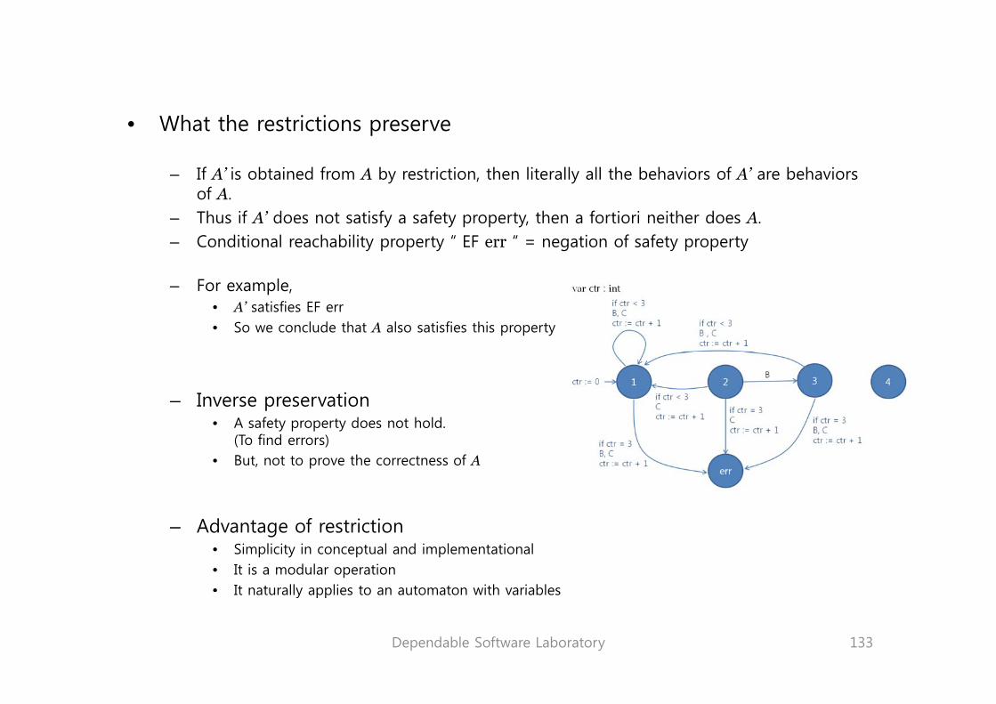
• What the restrictions preserve

– If A’ is obtained from A by restriction, then literally all the behaviors of A’ are behaviors of Aof A.

– Thus if A’ does not satisfy a safety property, then a fortiori neither does A.– Conditional reachability property “ EF err “ = negation of safety property

– For example, • A’ satisfies EF err• So we conclude that A also satisfies this property

– Inverse preservation• A safety property does not hold.

(To find errors)• But, not to prove the correctness of A

– Advantage of restriction• Simplicity in conceptual and implementational• It is a modular operation• It naturally applies to an automaton with variables


It naturally applies to an automaton with variables

133

11 6 Observer Automata11.6 Observer Automata

Ob• Observer automata– Aiming at simplifying a system by restricting its legitimate behaviors to those accepted

by an automata outside the system, called observer automata.– Reduce the size of automata by restricting its behavior rather than its structure (statesReduce the size of automata by restricting its behavior rather than its structure (states

and transitions in restriction methods)– PLTL model checking algorithm (in Chapter 3) use the concept.

– An example• Supposed that a single A may occur to prove the property.

01 02A

B,C B,C

01 02

An observer automaton O


B,C B,C

01 02A

A b Oif ctr < 3

if ctr < 3B, C

ctr := ctr + 1

var ctr : int;

if ctr < 3B CAn observer automaton O

102

202

302

B

B , C ctr := ctr + 1

B, Cctr := ctr + 1

SynchronizationB

if ctr < 3C

ctr := ctr + 1 if ctr = 3C

ctr := ctr + 1

if ctr = 3B, C

ctr := ctr + 1

101

ctr := 0

A

if t 3var ctr: int; Err

02

if ctr = 3B, C

ctr := ctr + 1Err01

if ctr = 3B, C

ctr := ctr + 1

The synchronized digicode with its observer

Dependable Software LaboratoryAn automaton A for the digicode

135


Part III. Some Tools


6 l d i h i l li i d i• 6 tools, concerned with a particular application domain– SMV– SPIN– DESIGN/CPN– UPPAAL– KRONOS– HYTECH


Chapter 12. SMV – Symbolic Model Checking

Chapter 13. SPIN – Communicating Automata

Chapter 14. DESIGN/CPN – Colored Petri Nets

Chapter 15. UPPAAL – Timed Automata

Ch t 16 KRONOS M d l Ch ki fChapter 16. KRONOS – Model Checking of Real-time Systems

Chapter 17. HYTECH – Linear Hybrid Systems


“Formal Modeling and Verification of Safety-Critical Software implemented in PLC”- IEEE Software, May/June, 2009.

정형 요구사항 명세 기반정형 요구사항 명세 기반원자력 소프트웨어 개발 방법론

D d bl S ft L b tDependable Software Laboratory

KONKUK University, Korea


2010.05.25



SMV를 이용한SMV를 이용한NuSCR 정형명세에 대한 정형검증

Dependable Software LaboratoryKonkuk UniversityKonkuk University


2010.05.25



SPIN을 이용한SPIN을 이용한MOST NS 프로토콜 정형검증

이동아 학생의 연구내용 삽입 요망



UPPAAL을 이용한UPPAAL을 이용한커피자판기 정형명세 및 정형검증

2009 건국대학교 대학원고급소프트웨어공학 수업

팀프로젝트 T2 / T5



Documents

Model-Checking Techniques and Tools