MODEL CALCULATIONS OF SHORT-TERM FORECASTS OF …

MODEL CALCULATIONS OF SHORT-TERM FORECASTS OF RUSSIAN ECONOMIC TIME SERIES

04 / 2020

2358

1010111112

M.Turuntseva, E.Astafieva, M.Bayeva, A.Bozhechkova, A.Buzaev, T.Kiblitskaya, Yu.Ponomarev and A.Skrobotov

INTRODUCTION TO ALL THE ISSUES INDUSTRIAL PRODUCTION AND RETAIL SALES FOREIGN TRADE INDEXES DYNAMICS OF PRICES MONETARY INDEXES INTERNATIONAL RESERVES FOREIGN EXCHANGE RATES THE LIVING STANDARD INDEXES EMPLOYMENT AND UNEMPLOYMENT ANNEXS 13

04/ 2

020

MODEL CALCULATIONS OF SHORT-TERM FORECASTS...

2

INTRODUCTION TO ALL THE ISSUES

This paper presents calculations of various economic indicators for the Russian Federation in May 2020 to October 20201, which were performed using time series models developed as a result of research con-ducted by the Gaidar Institute over the past few years.2 A method of forecasting falls within the group of formal or statistical methods. In other words, the calculated values neither express the opinion nor expert evaluation of the researcher, rather they are calculations of future values for a specific economic indicator, which were performed using formal ARIMA-models (p, d, q) given a prevailing trend and its, in some cases, significant changes. The presented forecasts are of inertial nature, because respective models rely upon the dynamics of the data registered prior to the moment of forecasting and depend too heavily on the trends, which are typical of the time series in the period immediately preceding the time horizon to be forecast. The foregoing calculations of future values of economic indicators for the Russian Federation can be used in making decisions on economic policy, provided that the general trends, which were seen prior to forecasting for each specific indicator, remain the same, i.e. prevailing long-term trends will see no serious shocks or changes in the future.

Despite that there is a great deal of data available on the period preceding the crisis of 1998, models of forecasting were analyzed and constructed using only the time horizon which followed August 1998. This can be explained by the findings of previous studies3, which concluded, among other key inferences, that the quality of forecasts was deteriorated in most of the cases when the data on the pre-crisis period was used. Additionally, it currently seems incorrect to use even shorter series (following the crisis of 2008), because statistical characteristics of models based on such a short time horizon are very poor.

Models for the economic indicators in question were evaluated using standard methods of time series analysis. Initially, the correlograms of the studied series and their first differences were analyzed in order to determine the maximum number of delayed values to be included into the specifications of a model. Then, the results of analyzed correlograms served as the basis for testing all the series for weak stationarity (or stationarity around the trend) using the Dickey–Fuller test. In some cases, the series were tested for stationarity around the segmented trend using Perron and Zivot–Andrews tests for endogenous structural changes.4

The series were broken down into weak stationary, stationary near the trend, stationary near the trend with structural change or difference stationary, and then models, which corresponded to each type (regarding the levels and including, if necessary, the trend or segmented trend or differences), were evaluated. The Akaike and Schwartz information criteria, the properties of models’ residuals (lack of autocorrelation, homoscedasticity and normality) and the quality of the in-sample-forecasts based on these models were used to choose the best model. Forecast values were calculated for the best of the models constructed for each economic indicator.

Additionally, the Bulletin presents future monthly values of the CPI, which were calculated using models developed at the Gaidar Institute, and volumes of imports/exports from/to all countries, which were calculated using structural models (SM). The forecast values based on the structural models may, in some cases, produce better results than ARIMA-models do, because structural models are constructed by adding information of the dynamics of exogenous variables. Besides, the use of structural forecasts in making aggregated forecasts (i.e. forecasts obtained as average value from several models) may help make forecast values more accurate.

1 Given that from early 2019 Rosstat does not release monthly data on indexes of real disposable cash income of the popula-tion, commencing from issue 8/2019 we release forecasts in quarter terms for 2 quarters ahead.

2 See, for example, R.M. Entov, S.M. Drobyshevsky, V.P. Nosko, A.D. Yudin. The Econometric Analysis of the Time Series of the Main Macroeconomic Indexes. Moscow, IET, 2001; R.M. Entov, V.P. Nosko, А.D. Yudin, P.А. Kadochnikov, S.S. Ponomarenko. Problems of Forecasting of Some Macroeconomic Indexes. Moscow, IET, 2002; V. Nosko, А. Buzaev, P. Kadochnikov, S. Ponomarenko. Analysis of the Forecasting Parameters of Structural Models and Models with the Outputs of the Polls of Industries. Moscow, IET, 2003; M.Yu. Turuntseva and T.R. Kiblitskaya, Qualitative Properties of Different Approaches to Forecasting of Social and Economic Indexes of the Russian Federation. Moscow, IET, 2010.

3 Ibid.4 See.: Perron, P. Further Evidence on Breaking Trend Functions in Macroeconomic Variables, Journal of Econometrics, 1997,

80, pp. 355–385; Zivot, E. and D.W.K. Andrews. Further Evidence on the Great Crash, the Oil-Price Shock, and Unit-Root Hypothesis. Journal of Business and Economic Statistics, 1992, 10, pp. 251–270.

3

04/ 2

020

INDUSTRIAL PRODUCTION AND RETAIL SALES

The dynamics of the Consumer Price Index was modeled using theoretical assumptions arising from the monetary theory. The following was used as explanatory variables: money supply, output volume, the dy-namics of the ruble-dollar exchange rate, which reflects the dynamics of alternative cost of money-keeping. The model for the Consumer Price Index also included the price index in the electric power industry, because the dynamics of manufacturers’ costs relies heavily on this indicator.

The baseline indicator to be noted is the real exchange rate, which can influence the value of exports and imports, and its fluctuations can result in changes to the relative value of domestically-produced and imported goods, though the influence of this indicator turns out to be insignificant in econometric models. Global prices of exported resources, particularly crude oil prices, are most significant factors, which deter-mine the dynamics of exports: a higher price leads to greater exports of goods. The level of personal income in the economy (labor costs) was used to describe the relative competitive power of Russian goods. Fictitious variables D12 and D01 – equal to one in December and January and zero in other periods – were added so that seasonal fluctuations were factored in. The dynamics of imports is effected by personal and corporate incomes whose increase triggers higher demand for all goods including imported ones. The real disposable cash income reflects the personal income; the Industrial Production Index reflects the corporate income.

The forecast values of foreign exchange rates were also calculated using structural models of their dependence on global crude oil prices.

The forecast values of explanatory variables, which are required for forecasting on the basis of structur-al models, were calculated using ARIMA-models (p, d, q).

The paper also presents calculations of the values of the Industrial Production Index, the Producer Price Index and the Total Unemployment Index, which were calculated using the results of business surveys conducted by the Gaidar Institute. Empirical studies show1 that the use of series of business surveys as explanatory variables 2 in forecasting models can make forecasting more accurate on the average. Future values of these indicators were calculated using ADL-models (seasonal autoregressive delays were added).

The Consumer Price Index and the Producer Price Index are also forecast using large datasets (factor models – FM). The construction of factor models relies basically on the evaluation of the principal com-ponents of a large dataset of socio-economic indicators (112 indicators in this case). The lags of these principal components and the lags of the explanatory variable are used as explanatory variables in these models. A quality analysis of the forecasts obtained for different configurations of the factor models was used to choose a model for the CPI, which included 9th, 12th and 13th lags of the four principal components, as well as 1st and 12th lags of the variable itself, and a model for the PPI, which included 8th, 9th and 12th lags of the four principal components, as well as 1st, 3rd and 12th lags of the variable itself.

All calculations were performed using the Eviews econometric package.

INDUSTRIAL PRODUCTION AND RETAIL SALES Industrial productionFor making forecast for May to October 2020, the series of monthly data of the indexes of industrial production released by the Federal State Statistics Service (Rosstat) from January 2002 to February 2020, as well as the series of the base indexes of industrial production released by the National Research University Higher School of Economics (NRU HSE3) over the period from January 2010 to March 2020 were used (the corrected value of January 2010 was equal to 100%). The forecast values of the series were calculated on the basis of ARIMA-class models. The forecast values of the Rosstat and the NRU HSE industrial production indexes are calculated using business surveys (BS) as well. The obtained results are shown in Table 1.

1 See, for example: V. Nosko, А. Buzaev, P. Kadochnikov, S. Ponomarenko. The Analysis of Forecasting Parameters of Structural Models and Models with Business Surveys’ Findings. Moscow, IEP, 2003.

2 Used as explanatory variables were the following series of the business surveys: the current/expected change in production, the expected changes in the solvent demand, the current/expected price changes and the expected change in employment.

3 The indexes in question are calculated by E.F. Baranov and V.A. Bessonov.

04/ 2

020


4

Tabl

e 1

Calc

ulat

ions

of f

orec

ast v

alue

s of

the

indu

stria

l pro

duct

ion

inde

xes1 (

%)

Index of industrial production

IIP for mining

IIP for manufacturing

IIP for utilities (electrici-ty, water, and gas)

IIP for food products

IIP for coke and petro-leum

IIP for primary metals and fabricated metal

products

IIP for machinery

Ross

tat

NRU

HSE

Rosstat

NRU HSE

Rosstat

NRU HSE

Rosstat

NRU HSE

Rosstat

NRU HSE

Rosstat

NRU HSE

Rosstat

NRU HSE

Rosstat

NRU HSE

ARIMA

BS

ARIMA

BSEx

pect

ed g

row

th o

n th

e re

spec

tive

mon

th o

f the

pre

viou

s ye

arM

ay 2

020

3.3

-5.0

2.7

-3.5

3.1

-0.3

5.2

5.5

-0.4

-3.5

3.3

4.0

5.5

8.8

-4.5

-2.3

7.6

8.1

June

202

02.

9-0

.22.

41.

43.

5-1

.13.

63.

7-1

.0-4

.25.

54.

34.

34.

8-6

.0-2

.80.

9-0

.9Ju

ly 2

020

2.3

-1.1

2.1

0.5

2.3

1.4

2.6

2.2

-0.9

-4.4

0.6

2.0

0.1

-1.2

-4.4

-0.7

12.0

-1.7

Augu

st 2

020

2.2

-2.0

1.4

-0.4

0.9

1.5

3.1

0.7

-1.5

-4.7

3.3

1.9

0.3

-1.6

-10.

3-6

.38.

5-2

.9Se

ptem

ber 2

020

1.8

0.2

1.2

1.8

0.2

1.5

2.6

0.9

-1.8

-5.3

2.4

1.1

0.8

1.4

-4.5

-6.3

3.3

-7.2

Oct

ober

202

01.

3-0

.40.

90.

40.

71.

42.

2-0

.9-0

.6-7

.92.

90.

61.

2-1

.5-4

.7-6

.61.

2-1

.7Fo

r ref

eren

ce: a

ctua

l gro

wth

in 2

019

on t

he re

spec

tive

mon

th o

f 201

8M

ay 2

019

-0.1

-0.4

2.9

2.6

-2.7

-2.9

1.3

-1.6

1.5

1.2

-4.5

-6.4

0.2

-0.1

5.2

6.5

June

201

91.

90.

62.

21.

81.

90.

01.

7-0

.51.

00.

9-3

.3-5

.56.

95.

58.

38.

3Ju

ly 2

019

2.8

1.5

2.0

1.8

3.7

1.6

0.9

0.6

6.8

3.9

1.0

0.0

-1.1

-2.4

13.6

11.9

Augu

st 2

019

2.8

2.4

2.1

1.8

3.4

3.2

1.1

1.3

1.3

2.4

4.5

4.9

6.2

4.4

4.8

2.7

Sept

embe

r 201

93.

82.

51.

40.

95.

94.

13.

75.

36.

14.

91.

2-0

.63.

82.

57.

81.

0O

ctob

er 2

019

3.0

1.3

-0.7

-0.8

6.3

3.6

2.0

2.5

4.4

3.1

7.0

4.1

-0.6

-2.4

17.2

16.8

Not

e. In

the

time

span

s un

der r

evie

w, t

he s

erie

s of

the

Ross

tat a

nd th

e N

RU H

SE c

hain

inde

xes

of II

P, as

wel

l as

the

NRU

HSE

cha

in II

P fo

r man

ufac

turin

g ar

e id

entifi

ed a

s st

atio

nary

pro

cess

es

arou

nd th

e tr

end

with

an

endo

geno

us s

truc

tura

l cha

nge;

the

serie

s of

the

Ross

tat a

nd th

e N

RU H

SE c

hain

IIPs

for m

anuf

actu

ring,

for p

rimar

y m

etal

s an

d fa

bric

ated

met

al p

rodu

cts,

as w

ell

as th

e N

RU H

SE c

hain

IIP

for m

inin

g an

d Ro

ssta

t cha

in II

P fo

r mac

hine

ry a

nd e

quip

men

t are

iden

tified

as

stat

iona

ry p

roce

sses

aro

und

the

tren

d w

ith tw

o en

doge

nous

str

uctu

ral c

hang

es. T

he

time

serie

s of

oth

er c

hain

inde

xes

are

stat

iona

ry a

t lev

els.

1 It

is to

be

note

d th

at fo

r mak

ing

of fo

reca

sts

so-c

alle

d “r

aw” i

ndex

es (w

itho

ut s

easo

nal a

nd c

alen

dar a

djus

tmen

t) w

ere

used

and

for t

hat r

easo

n in

mos

t mod

els

exis

tenc

e of

the

sea

son

fact

or is

tak

en in

to a

ccou

nt a

nd, a

s a

cons

eque

nce,

the

obt

aine

d ou

tput

s re

flect

the

sea

sona

l dyn

amic

s of

the

ser

ies.

5

04/ 2

020

FOREIGN TRADE INDEXES

As seen from Table 1, the Rosstat average1 growth in the industrial production index in May-October 2020 compared to the same period of the previous year for the industry as a whole comes to 0.4%. The NRU HSE industrial production index comes to 0.9%. To note that forecasts on ARIMA-models demonstrate increment in both IPP and on business models – decrease.

The average monthly gain in the Rosstat and the NRU HSE industrial production indexes for mining and quarrying amount to 1.8% and 0.7%, respectively in May-October 2020.

The average gain in the Rosstat industrial production index in manufacturing industry for May-October 2020 amounts to 3.2% compared to the same period of the previous year and the NRU HSE industrial production index in manufacturing industry comes to 2.0%. The average monthly increase in production of food products to average by 3.0% and 2.3% for the Rosstat and NRU HSE indexes, respectively. The pro-duction of coke and petroleum products is forecast to grow on average by 2.0% and 1.8% for the Rosstat and NRU HSE indexes, respectively. The average monthly change in the industrial production index for primary metals and fabricated metal products for May-October 2020 computed by Rosstat and the NRU HSE constitutes -5.7% and -4.2%, respectively. Manufacturing of machinery and equipment is forecast to grow on average by 5.6% and 1.0% for the Rosstat and the NRU HSE indexes, respectively.

The average gain in the Rosstat industrial production index for electricity, gas, and steam supply; for air conditioning in May-October 2020 constitutes -1.0% in comparison with the same period of the previous year; the same indicator for the NRU HSE industrial production index comes to -5.0%.

Retail SalesThis section (Table 2) presents forecasts of monthly retail sales made on the basis of monthly Rosstat data over January 1999 – April 2020.

As seen from Table 2, the average forecast decrease in the monthly turnover for May-October 2020 against the corresponding period of 2019 amounts to around 6.1%. The average forecast drop in the monthly real turnover for the period May-October 2020 compared to the same period of 2019 constitutes 8.1%.

FOREIGN TRADE INDEXESModel calculations of forecast values of the export, export to countries outside the CIS and the import, import from countries outside the CIS were made on the basis of the models of time series and structural models evaluated on the basis of the monthly data over the period from September 1998 to April 2020 on the basis of the data released by the Central Bank of Russia.2 The results of calculations are presented in Table 3.

Export, import, export outside the CIS and import from the countries outside the CIS are forecast to increase on average at 17.8%, -9.2%, -17.8%, and -9.4%, respectively for May-October 2020 against May- October 2019. The average forecast trade balance volume with all countries for May-October 2020 will total $48.0 bn, which corresponds to a decrease by 36.6% in relation to May-October 2019.

1 Average growth of industrial production indexes is the average value of these indexes for six months under review.2 The data on the foreign trade turnover is calculated by the CBR in accordance with the methods for making of the balance of

payment in prices of the exporter-country (FOB) in billion USD.

Table 2Calculations of forecast values of retail sales and real retail sales

Forecast value according to ARIMA-model Retail sales, billion RUB (in brackets –

growth on the respective month of the previous year, %)

Real retail sales (as % of the

respective period of the previous

year)May 2020 2104.2 (-20.8) 78.9June 2020 2464.2 (-10.1) 88.7July 2020 2689.1 (-4.2) 93.4August 2020 2836.7 (-2.1) 95.5September 2020 2853.3 (-0.1) 96.8October 2020 2933.6 (1.0) 98.2For reference: actual values in the same months of 2019

May 2019 2656.9 101.9June 2019 2741.0 101.8July 2019 2807.0 101.5August 2019 2897.5 101.1September 2019 2856.2 100.9October 2019 2904.6 101.9

Note. The series of retail sales and real retail sales over January 1999 – April 2020.

04/ 2

020


6

Tabl

e 3

Calc

ulat

ions

of f

orec

ast v

alue

s of

vol

umes

of f

orei

gn tr

ade

turn

over

with

cou

ntrie

s ou

tsid

e th

e CI

S

Mon

th

Expo

rts

to a

ll co

untr

ies

Impo

rts

from

all

coun

trie

sEx

port

s to

cou

ntrie

s ou

tsid

e th

e CI

SIm

port

s fr

om c

ount

ries

outs

ide

the

CIS

Forecast values (billion USD a month)

Percentage of actual data in the respective month

of the previous year










ARIM

ASM

ARIM

ASM

ARIM

ASM

ARIM

ASM

ARIM

ASM

ARIM

ASM

ARIM

ASM

ARIM

ASM

May

202

025

.627

.979

8618

.918

.195

9122

.523

.980

8516

.816

.696

94Ju

ne 2

020

26.8

29.1

8390

18.4

19.0

9295

24.0

25.1

8690

17.1

17.3

9798

July

202

024

.328

.173

8420

.219

.890

8924

.624

.485

8518

.717

.794

89Au

gust

202

028

.928

.684

8320

.419

.693

8923

.224

.378

8217

.216

.688

85Se

ptem

ber

2020

29.1

29.5

8283

21.0

20.2

100

9624

.025

.078

8117

.817

.295

92

Oct

ober

202

030

.528

.483

7719

.020

.080

8424

.825

.778

8017

.517

.881

83Fo

r ref

eren

ce: a

ctua

l val

ues

in re

spec

tive

mon

ths

of 2

019

(bill

ion

USD

)M

ay 2

019

32.4

19.9

28.0

17.6

June

201

932

.420

.028

.017

.6Ju

ly 2

019

33.4

22.4

28.8

19.9

Augu

st 2

019

34.4

22.0

29.6

19.6

Sept

embe

r 20

1935

.521

.030

.818

.7

Oct

ober

201

936

.823

.932

.021

.5N

ote.

Ove

r the

per

iod

from

Janu

ary

1999

to A

pril

2020

, the

ser

ies

of e

xpor

ts, i

mpo

rts,

expo

rts

to th

e co

untr

ies

outs

ide

the

CIS

and

impo

rts

from

the

coun

trie

s ou

tsid

e th

e CI

S w

ere

iden

tified

as

sta

tiona

ry s

erie

s in

the

first

-ord

er d

iffer

ence

s. In

all

the

case

s, se

ason

al c

ompo

nent

s w

ere

incl

uded

in th

e sp

ecifi

catio

n of

the

mod

els.

7

04/ 2

020

DYNAMICS OF PRICESTa

ble

4Ca

lcul

atio

ns o

f for

ecas

t val

ues

of p

rice

inde

xes

Mon

th

The consumer price index (ARIMA)

The consumer price index (SM)

The consumer price index (FM)

Prod

ucer

pri

ce in

dexe

s:

for industrial goods (ARIMA)

for industrial goods (BS)

for industrial goods (FM)

for mining and quarrying

for manufacturing

for utilities (electricity, water, and gas)

for food products

for textile and sewing industry

for wood products

for pulp and paper industry

for coke and refined petroleum

for chemical industry

for basic metals and fabricated metal

for machinery and equipment

for transport equipment manufacturing

Fore

cast

val

ues

(% o

f the

pre

viou

s m

onth

)M

ay 2

020

100.

310

0.6

100.

410

0.6

93.9

100.

410

1.2

99.6

100.

310

0.9

99.6

100.

999

.310

1.8

98.5

101.

210

0.1

100.

6Ju

ne 2

020

100.

310

0.5

100.

499

.894

.810

0.5

99.4

99.2

100.

010

0.8

99.2

100.

810

0.2

103.

798

.610

1.1

100.

110

0.8

July

202

010

0.3

100.

310

0.4

100.

195

.2%

100.

597

.399

.710

0.5

101.

199

.110

0.3

99.7

102.

298

.610

1.3

100.

210

0.6

Augu

st 2

020

100.

110

0.1

100.

310

0.2

95.9

100.

510

1.3

99.8

102.

110

0.6

99.5

100.

799

.810

3.0

98.4

101.

510

0.3

100.

0Se

ptem

ber

2020

100.

210

0.2

100.

510

0.2

97.0

100.

510

1.5

100.

310

0.0

100.

798

.710

0.4

100.

310

2.2

98.3

100.

610

0.2

100.

2

Oct

ober

202

010

0.4

100.

310

0.5

99.9

97.3

100.

598

.410

0.1

100.

410

0.9

99.5

100.

099

.910

2.6

98.4

101.

010

0.2

101.

0Fo

reca

st v

alue

s (%

of D

ecem

ber 2

019)

May

202

010

1.6

102.

710

0.8

101.

410

2.1

101.

497

.310

0.1

102.

010

3.2

97.8

103.

196

.110

5.0

94.6

103.

710

0.8

102.

7Ju

ne 2

020

102.

010

3.2

100.

810

1.2

101.

010

1.5

96.7

99.3

102.

010

4.0

97.0

103.

996

.310

8.8

93.3

104.

810

1.0

103.

5Ju

ly 2

020

102.

310

3.6

100.

810

1.3

100.

410

1.5

94.1

99.0

102.

510

5.2

96.0

104.

396

.011

1.2

91.9

106.

210

1.1

104.

2Au

gust

202

010

2.4

103.

710

0.7

101.

510

0.7

101.

595

.498

.910

4.7

105.

895

.510

5.0

95.8

114.

690

.510

7.7

101.

410

4.2

Sept

embe

r 20

2010

2.6

103.

910

0.9

101.

710

1.1

101.

596

.899

.110

4.7

106.

694

.310

5.4

96.1

117.

189

.010

8.4

101.

610

4.4

Oct

ober

202

010

3.0

104.

210

0.9

101.

610

0.3

101.

595

.399

.210

5.1

107.

693

.810

5.4

96.0

120.

287

.610

9.5

101.

810

5.5

For r

efer

ence

: act

ual v

alue

s in

the

sam

e pe

riods

of 2

019

(% o

f Dec

embe

r 201

8)M

ay 2

019

102.

310

1.3

104.

999

.710

1.9

99.1

101.

010

0.4

100.

394

.798

.610

0.6

101.

910

2.6

June

201

910

2.3

100.

710

3.1

99.7

100.

999

.010

0.9

100.

099

.994

.898

.310

0.5

102.

010

3.3

July

201

910

2.5

97.9

92.4

99.4

102.

399

.310

1.2

99.0

98.5

92.8

97.1

100.

610

2.2

103.

1Au

gust

201

910

2.3

97.4

91.7

98.7

102.

799

.299

.598

.696

.789

.295

.710

0.9

102.

810

2.7

Sept

embe

r 20

1910

2.1

97.1

91.3

98.7

101.

698

.699

.298

.595

.989

.594

.810

0.8

102.

710

2.8

Oct

ober

201

910

2.2

96.9

90.1

98.7

102.

198

.410

0.6

97.8

95.5

90.2

94.0

100.

410

2.8

102.

8N

ote.

Ove

r the

per

iod

from

Janu

ary

1999

to M

arch

202

0, th

e se

ries

of th

e ch

ain

prod

ucer

pric

e in

dex

for m

achi

nery

are

iden

tified

as

a st

atio

nary

pro

cess

aro

und

the

tren

d w

ith tw

o en

dog-

enou

s st

ruct

ural

cha

nges

. The

ser

ies

of o

ther

cha

in p

rice

inde

xes

are

stat

iona

ry a

t lev

els.

04/ 2

020


8

DYNAMICS OF PRICESThe Consumer Price Index and Producer Price IndexThis section presents calculations of forecast values of the consumer price index and producer price index (as regards both the industry in general and some types of its activities under the National Industry Classification Standard (NICS)) made on the basis of the time-series models evaluated on the basis of the data released by Rosstat over the period from January 1999 to March 2020.1 Table 4 presents the results of model calculations of forecast values over May to October of 2020 in accordance with ARIMA-models, structural models (SM) and models computed with the help of business surveys (BS).

The forecast average monthly increment in the consumer price index in May-October 2020 will come to 0.3%. The producer price index for industrial goods for the same period is forecast to drop on average 1.2% per month.

The Rosstat producer price indexes are forecast to grow at average monthly rate for May-October 2020: for mining and quarrying (-0.1%), manufacturing (-0.2%), utilities (electricity, gas, and steam) 0.5%, food products 0.8%, textile and sewing industry (-0.8%), wood products 0.5%, pulp and paper industry (-0.1%), coke and refined petroleum 2.6%, for chemical industry (-1.5%), for basic metals and fabricated metal 1.1%, for machinery and equipment 0.2%, and for motor vehicles manufacture 0.6%.

The Cost of the Monthly per Capita Minimum Food BasketThis section presents calculations of forecast values of the cost of the monthly per capita minimum food basket over May to October 2020. The forecasts were made on the basis of time series with the use of the Rosstat data over the period from January 2000 to April 2020. The results are presented in Table 5.

As can be seen from Table 5, the minimum set of food products’ cost is forecast to grow compared to the corresponding level of the previous year. Having said that, the minimum set of food products is forecast to average RUB 4,370.4. The minimum set of food prod-ucts’ cost is forecast to grow on average at around 3.7% against the same period of last year.

Indexes of Freight Rates This section presents calculations of forecast values of freight tariff indexes on cargo carriage,2 made on the basis of time-series models evaluated on the Rosstat data over the period from September 1998 to January 2020. Table 6 shows the results of model calculations of forecast values in the May-October of 2020. It should be noted that some of the indexes under review (for instance, the index of pipeline tariff) are adjustable ones and for that reason their behavior is hard to describe by means of the time-series models. As a result, the future values may differ greatly from the real ones in case of the centralized increase in tariffs in the period of forecasting or in case of absence of such an increase in the forecasting period, but with it taking place shortly before the beginning of that period.

1 Structural models were evaluated in the period from October 1998.2 The paper presents a review of the composite freight rate index on freight transport and the motor load freight rate index,

as well as the pipeline rate index. The composite freight rate index is computed on the basis of the freight rate indexes by individual types of transport: rail, pipeline, shipping, domestic water-borne, and motor load freight and air service (for more detailed information, pls. refer, for instance, to: Pr ices in Russia . The Official Publication of Goskomstat of RF, 1998).

Table 5The forecast of the cost of the monthly per capita minimum food basket

Forecast values according to ARIMA-model (RUB)

May 2020 4462.6June 2020 4504.0July 2020 4483.3August 2020 4324.0September 2020 4230.7October 2020 4217.9For reference: actual values in the same

months of 2019 (billion RUB)May 2019 4356.6June 2019 4367.0July 2019 4311.7August 2019 4170.0September 2019 4062.7October 2019 4022.6

Expected growth on the respective month of the previous year (%)

May 2020 2.4June 2020 3.1July 2020 4.0August 2020 3.7September 2020 4.1October 2020 4.9

Note. The series of the cost of the monthly per capita minimum food basket over the period from January 2000 April 2020 are stationary in the first-order differences.

9

04/ 2

020

DYNAMICS OF PRICES

According to the forecast results for May-October 2020, the composite index of transport tariffs on freight carriage during these six months will be growing at an average monthly rate of 0.3%. In April 2020, seasonal growth in the index is expected at 3.1 p.p. and in October a seasonal decline – at 4.6 p.p.

The index of motor freight tariffs will be decreasing during these six months at an average monthly rate of 0.3%.

The index of pipeline tariffs will be decreasing at an average monthly rate of 0.2%. In July 2020, seasonal growth in the index is expected at 2.7 p.p. and in October a seasonal decline – at 3.7 p.p.

World Prices of Natural ResourcesThis section presents calculations of such average monthly values of Brent crude prices (US$ per barrel), the aluminum prices (US$ per ton), the gold prices ($ per ounce), the copper prices (US$ per ton), and the nickel prices (US$ per ton) over April to September 2020 as were received on the basis of nonlinear models of time series evaluated on the basis of the IMF data over the period from January 1980 to March 2020.

The crude oil price is forecast to average around $18.9 per barrel, which is below its corresponding year-earlier indexes on average by 69.9%. The aluminum prices are forecast to average around $1,366 per ton and their average forecast decline constitutes around 22% compared to the same level of last year. The gold price is forecast to average $1,648 per ounce. The copper price is forecast to average $4,527 per ton, and prices for nickel – around $10,552 per ton. The average forecast price increase in gold constitutes around 16%, the average decline in copper prices – around 22%, nickel prices – 29% against the corre-sponding level of last year.

Table 6Calculations of forecast values of freight tariffs indexes

Month

The com-posite index of transport

tariff

The index of motor

freight tariff

The index of pipeline

tariff

Forecast values according to ARIMA-models(% of the previous month)

May 2020 99.8 99.7 100.4June 2020 99.8 99.7 100.2July 2020 103.1 99.7 102.7August 2020 99.8 99.7 102.6September 2020 99.8 99.6 96.8October 2020 95.4 99.6 96.3

Forecast values according to ARIMA-models(% of December of the previous year)

May 2020 102.1 98.8 93.2June 2020 101.9 98.5 93.6July 2020 105.1 98.2 93.8August 2020 104.9 97.9 96.3September 2020 104.7 97.5 98.8October 2020 99.9 97.2 95.7For reference: actual values in the same period of 2019

(% of the previous month)May 2019 100.0 100.0 100.1June 2019 99.9 100.0 99.9July 2019 103.1 100.0 107.6August 2019 100.2 100.1 100.3September 2019 99.9 100.0 99.8October 2019 95.8 100.0 90.1

Note. Over the period from September 1998 to January 2020, the series of the freight tariff index were identified as station-ary ones; the other series were identified as stationary ones over the period from September 1998 to January 2020, too; fictitious variables for taking into account particularly dramat-ic fluctuations were used in respect of all the series.

Table 7Calculations of forecast values of world prices on natural resources

Month

Bren

t oil

($ p

er b

arre

l)

Alum

inum

($

per

ton)

Gol

d ($

per

oun

ce)

Copp

er

($ p

er to

n)

Nic

kel

($ p

er to

n)

Forecast valuesMay 2020 18.87 1431 1611 4560 10887June 2020 18.37 1382 1638 4528 10794July 2020 19.32 1352 1647 4501 10528August 2020 19.29 1361 1647 4510 10410September 2020 18.89 1343 1663 4522 10348October 2020 18.81 1330 1685 4540 10342

Expected growth on the respective month of the previous year (%)

May 2020 -70.7 -19.5 25.5 -21.7 -9.2June 2020 -72.4 -22.5 20.5 -24.5 -14.8July 2020 -70.4 -24.2 16.5 -24.2 -27.7August 2020 -68.1 -21.4 9.9 -20.2 -41.8September 2020 -68.9 -21.4 10.0 -20.8 -39.5October 2020 -68.8 -24.5 12.7 -21.8 -38.0

For reference: actual values in the same period of 2019May 2019 64.49 1778 1284 5823 11990June 2019 66.55 1782 1359 6001 12675July 2019 65.17 1782 1413 5935 14553August 2019 60.43 1733 1499 5652 17900September 2019 60.78 1708 1511 5710 17110October 2019 60.23 1762 1495 5806 16690

Note. Over the period from January 1980 to March 2020, the series of prices of crude oil, nickel, gold, copper, and aluminum are series of DS type.

04/ 2

020


10

MONETARY INDEXESThe future values of the monetary base (in the narrow definition: cash funds and the Fund of Man-datory Reserves (FMR) and М2 monetary aggregate over the period from April to September 2020 were received on the basis of models of time-series of re-spective indexes calculated by the CBR1 in the period from October 1998 to March 2020 for the monetary base and to February 2020 for M2 monetary. Table 8 presents the results of calculations of forecast val-ues and actual values of those indexes in the same period of previous year. It is to be noted that due to the fact that the monetary base is an instrument of the CBR policy, forecasts of the monetary base on the basis of time-series models are to a certain extent notional as the future value of that index is determined to a great extent by decisions of the CBR, rather than the inherent specifics of the series.

In May-October 2020, in the period under re-view the monetary base will be growing at an average monthly rate of 0.6%. In the period under review, M2 monetary index will not be changing.

INTERNATIONAL RESERVESThis section presents the outputs of the statistical estimation of such future values of the international reserves of the Russian Federation2 as were received on the basis of evaluation of the model of time series of the gold and foreign exchange reserves on the basis of the data released by the CBR over the period from October 1998 to February of 2020. That index is forecast without taking into account a decrease in the amount of reserves due to foreign debt payment and for that reason the values of the volumes of the international reserves in the months where foreign debt payments are made may happen to be overes-timated (or otherwise underestimated) as compared to the actual ones.

Subsequent to the forecast findings for May-October 2020, the international reserves will be growing at an average monthly rate of 0.6%.

1 The data on the specific month is given in accordance with the methods of the CBR as of the beginning of the following month.

2 The data on the volume of the gold and foreign exchange reserves is presented as of the first day of the following month.

Table 8The forecast of M2 and the monetary base

Month

The monetary base M2

Billion RUB

Growth on the previous

month, %

Billion RUB

Growth on the previous

month, %

May 2020 10942 1.2 50987 0.7June 2020 10951 0.1 50612 -0.7July 2020 11083 1.2 50987 0.7August 2020 11093 0.1 50611 -0.7September 2020 11226 1.2 50987 0.7October 2020 11238 0.1 50611 -0.7For reference: actual value in the respective months of 2019

(growth on the previous month, %)May 2019 2.3 0.6June 2019 -0.9 0.6July 2019 0.9 1.3August 2019 0.4 0.0September 2019 1.3 0.5October 2019 0.4 1.4

Note. Over the period from October 1998 to March 2020, the time series of monetary base were attributed to the class of series which are stationary in the first-order differences and have an explicit seasonal component and the time series of M2 monetary aggregate from October 1998 to February 2020 was identified as stationary series with explicit seasonal component.

Table 9The forecast of the international reserves of the Russian Federation

Month

Forecast values according to ARIMA-model

Billion USD Growth on the previous month, %

May 2020 576.2 0.6June 2020 579.3 0.5July 2020 582.6 0.6August 2020 586.1 0.6September 2020 589.5 0.6October 2020 592.9 0.6

For reference: actual values in the same period of 2019May 2019 491.1 0.7June 2019 495.2 0.8July 2019 518.4 4.7August 2019 519.8 0.3September 2019 529.1 1.8October 2019 530.9 0.3

Note. Over the period from October 1998 to February 2020, the series of the gold and foreign exchange reserves of the Russian Federation were identified as stationary series in difference.

11

04/ 2

020

FOREIGN EXCHANGE RATES

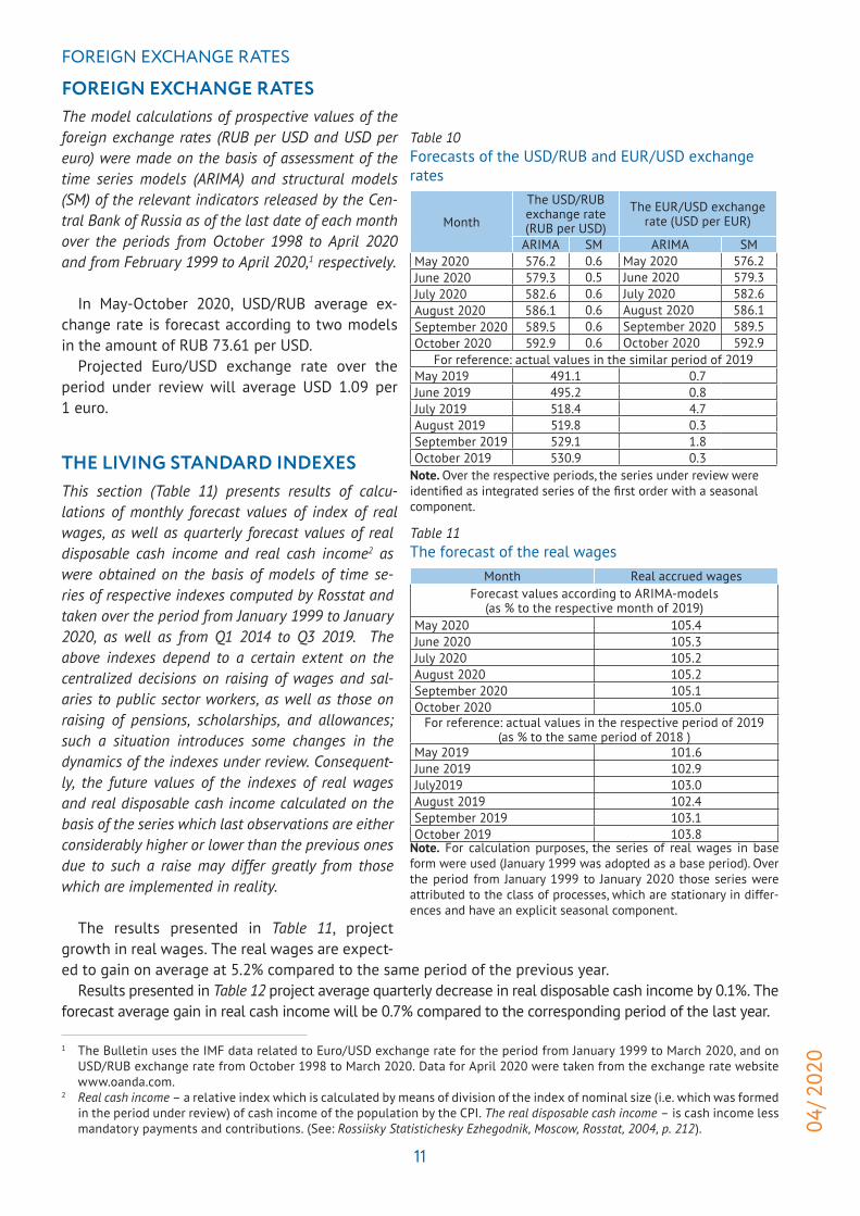
FOREIGN EXCHANGE RATESThe model calculations of prospective values of the foreign exchange rates (RUB per USD and USD per euro) were made on the basis of assessment of the time series models (ARIMA) and structural models (SM) of the relevant indicators released by the Cen-tral Bank of Russia as of the last date of each month over the periods from October 1998 to April 2020 and from February 1999 to April 2020,1 respectively.

In May-October 2020, USD/RUB average ex-change rate is forecast according to two models in the amount of RUB 73.61 per USD.

Projected Euro/USD exchange rate over the period under review will average USD 1.09 per 1 euro.

THE LIVING STANDARD INDEXESThis section (Table 11) presents results of calcu-lations of monthly forecast values of index of real wages, as well as quarterly forecast values of real disposable cash income and real cash income2 as were obtained on the basis of models of time se-ries of respective indexes computed by Rosstat and taken over the period from January 1999 to January 2020, as well as from Q1 2014 to Q3 2019. The above indexes depend to a certain extent on the centralized decisions on raising of wages and sal-aries to public sector workers, as well as those on raising of pensions, scholarships, and allowances; such a situation introduces some changes in the dynamics of the indexes under review. Consequent-ly, the future values of the indexes of real wages and real disposable cash income calculated on the basis of the series which last observations are either considerably higher or lower than the previous ones due to such a raise may differ greatly from those which are implemented in reality.

The results presented in Table 11, project growth in real wages. The real wages are expect-ed to gain on average at 5.2% compared to the same period of the previous year.

Results presented in Table 12 project average quarterly decrease in real disposable cash income by 0.1%. The forecast average gain in real cash income will be 0.7% compared to the corresponding period of the last year.

1 The Bulletin uses the IMF data related to Euro/USD exchange rate for the period from January 1999 to March 2020, and on USD/RUB exchange rate from October 1998 to March 2020. Data for April 2020 were taken from the exchange rate website www.oanda.com.

2 Real cash income – a relative index which is calculated by means of division of the index of nominal size (i.e. which was formed in the period under review) of cash income of the population by the CPI. The real disposable cash income – is cash income less mandatory payments and contributions. (See: Rossiisky Statistichesky Ezhegodnik, Moscow, Rosstat, 2004, p. 212).

Table 10Forecasts of the USD/RUB and EUR/USD exchange rates

Month

The USD/RUB exchange rate (RUB per USD)

The EUR/USD exchange rate (USD per EUR)

ARIMA SM ARIMA SMMay 2020 576.2 0.6 May 2020 576.2June 2020 579.3 0.5 June 2020 579.3July 2020 582.6 0.6 July 2020 582.6August 2020 586.1 0.6 August 2020 586.1September 2020 589.5 0.6 September 2020 589.5October 2020 592.9 0.6 October 2020 592.9

For reference: actual values in the similar period of 2019May 2019 491.1 0.7June 2019 495.2 0.8July 2019 518.4 4.7August 2019 519.8 0.3September 2019 529.1 1.8October 2019 530.9 0.3

Note. Over the respective periods, the series under review were identified as integrated series of the first order with a seasonal component.

Table 11The forecast of the real wages

Month Real accrued wagesForecast values according to ARIMA-models

(as % to the respective month of 2019)May 2020 105.4June 2020 105.3July 2020 105.2August 2020 105.2September 2020 105.1October 2020 105.0

For reference: actual values in the respective period of 2019 (as % to the same period of 2018 )

May 2019 101.6June 2019 102.9July2019 103.0August 2019 102.4September 2019 103.1October 2019 103.8

Note. For calculation purposes, the series of real wages in base form were used (January 1999 was adopted as a base period). Over the period from January 1999 to January 2020 those series were attributed to the class of processes, which are stationary in differ-ences and have an explicit seasonal component.

04/ 2

020


12

EMPLOYMENT AND UNEMPLOYMENTFor the purpose of calculation of the future values of employ-ment (the number of gainfully employed population) and the unemployment (the total number of unemployed), models of the time series evaluated over the period from October 1998 to February 2020 on the basis of the monthly data released by Rosstat1 were used. The unemployment was calculated on the basis of the models with results of the findings from business surveys2 too.It is to be noted that feasible logical inconsistencies3 in fore-casts of employment and unemployment which totals should be equal to the index of gainfully employed population may arise due to the fact that each series is forecast individually and not as a difference between the forecast values of gainfully employed population and another index.

Table 13Calculation of forecast values of employment and unemployment indexes

Month

Employment (ARIMA) Unemployment (ARIMA) Unemployment (BS)

Million people

Growth on the

respective month of previous year (%)

Million people

Growth on the


% of the index of

the number of the

gainfully employed population

Million people

Growth on the


% of the index of

the number of the

gainfully employed population

May 2020 71.8 0.3 3.2 -4.7 4.5 4.6 35.0 6.4June 2020 72.3 0.4 3.2 -4.0 4.4 4.4 32.5 6.1July 2020 72.5 0.5 3.3 -3.5 4.5 4.2 24.3 5.8August 2020 72.9 0.5 3.2 -2.3 4.4 4.1 25.5 5.6September 2020 72.6 0.5 3.3 -3.7 4.5 4.1 19.8 5.6October 2020 72.2 0.2 3.4 -3.1 4.7 4.0 15.5 5.5

For reference: actual values in the same periods of 2019 (million people)May 2019 71.6 3.4June 2019 72 3.3July 2019 72.2 3.4August 2019 72.5 3.3September 2019 72.2 3.4October 2019 72.1 3.5

Note. Over the period from October 1998 to February 2020, the series of employment is a stochastic process which is station-ary around the trend. The series of unemployment is a stochastic process with the first order integration. Both indexes include seasonal component.

According to ARIMA-model forecast (Table 13), in May-October 2020, the increase in the number of em-ployed in the economy will average 0.4% per month against the corresponding period of the previous year.

The average increase in the total number of unemployed is forecast at 11% per month against the same period of last year. To note that forecasts according to two models significantly differ: if the ARIMA-model forecasts decrease on average by 3.6% in the number of unemployed, while the business surveys model projects a notable growth in unemployed in the amount of 25.4% per month.

1 The index is computed in accordance with the methods of the International Labor Organization (ILO) and is given as of the month-end.

2 The model is evaluated over the period from January 1999 to January 2020.3 For example, deemed as such a difference may be a simultaneous decrease both in employment and unemployment. However,

it is to be noted that in principle such a situation is possible provided that there is a simultaneous decrease in the number of gainfully employed population.

Table 12The forecast of the living standard indexes

Period Real disposable cash income Real cash income

Forecast values according to ARIMA-models (as % to the corresponding quarter of 2019)

Q2 2020 100.2 101.0Q3 2020 99.5 100.4For reference: actual values for the respective

period of 2019 (in % to the same period of 2018)Q2 2019 101.0 101.5Q3 2019 103.1 103.7

13

04/ 2

020

ANNEXES

ANNEXES Annex 1. Diagrams of the Time Series of the Economic Indexes of the Russian Federation

Fig. 1а. The Rosstat industrial production index (ARIMA-model) (% of December 2001)

Fig. 1b. The NRU HSE industrial production index (ARIMA-model) (% of January 2010)

Fig. 2а. The Rosstat industrial production index for mining (% of December 2001)

Fig. 2b. The NRU HSE industrial production index for mining (% of January 2010)

04/ 2

020


14

Fig. 3а. The Rosstat industrial production index for manufacturing (% of December 2001)

Fig. 3b. The NRU HSE industrial production index for manufacturing (% of January 2010)

Fig. 4а. The Rosstat industrial production index for utilities (electricity, water, and gas) (as a percentage of that in December 2001)

Fig. 4b. The NRU HSE industrial production index for utilities (electricity, water, and gas) (as a percentage of that in January 2010)

15

04/ 2

020

ANNEXES Fig. 5а. The Rosstat industrial production index for food products (as a percentage of that in December 2001)

Fig. 5b. The NRU HSE industrial production index for food products (as a percentage of that in January 2010)

Fig. 6а. The Rosstat industrial production index for coke and petroleum (as a percentage of that in December 2001)

Fig. 6b. The NRU HSE industrial production index for petroleum and coke (as a percentage of that in January 2010)

04/ 2

020


16

Fig.7а. The Rosstat industrial production index for primary metals and fabricated metal products (as a percentage of that in December 2001)

Fig. 7b. The NRU HSE industrial production index for primary metals and fabricated metal products (as a percentage of that in January 2010)

Fig. 8а. The Rosstat industrial production index for machinery (as a percentage of that in December 2001)

Fig. 8b. The NRU HSE industrial production index for machinery (as a percentage of that in January 2010)

17

04/ 2

020

ANNEXES Fig. 9. The volume of retail sales (billion RUB)

2000.0

2200.0

2400.0

2600.0

2800.0

3000.0

3200.0

3400.0

3600.0

jan-

2017

feb-

2017

mar

-201

7ap

r-201

7m

ay-2

017

jun-

2017

jul-2

017

aug-

2017

sep-

2017

oct-2

017

nov-

2017

dec-

2017

jan-

2018

feb-

2018

mar

-201

8ap

r-201

8m

ay-2

018

jun-

2018

jul-2

018

aug-

2018

sep-

2018

oct-2

018

nov-

2018

dec-

2018

jan-

2019

feb-

2019

mar

-201

9ap

r-201

9m

ay-2

019

jun-

2019

jul-2

019

aug-

2019

sep-

2019

oct-2

019

nov-

2019

dec-

2019

jan-

2020

feb-

2020

mar

-202

0ap

r-202

0m

ay-2

020

jun-

2020

jul-2

020

aug-

2020

sep-

2020

oct-2

020

75.0

80.0

85.0

90.0

95.0

Fig. 9а. The real volume of retail sales (as a percentage of that in the same period of the previous year)

105.0

100.0

jan-

2015

feb-

2015

mar

-201

5ap

r-201

5m

ay-2

015

jun-

2015

jul-2

015

aug-

2015

sep-

2015

oct-2

015

nov-

2015

dec-

2015

jan-

2016

feb-

2016

mar

-201

6ap

r-201

6m

ay-2

016

jun-

2016

jul-2

016

aug-

2016

sep-

2016

oct-2

016

nov-

2016

dec-

2016

jan-

2017

feb-

2017

mar

-201

7ap

r-201

7m

ay-2

017

jun-

2017

jul-2

017

aug-

2017

sep-

2017

oct-2

017

nov-

2017

dec-

2017

jan-

2018

feb-

2018

mar

-201

8ap

r-201

8m

ay-2

018

jun-

2018

jul-2

018

aug-

2018

sep-

2018

oct-2

018

Fig.10. Export to all countries (billion USD)

Fig. 11. Export to countries outside the CIS (billion USD)

04/ 2

020


18

Fig. 12. Import from all countries (billion USD)

Fig. 13. Import from countries outside the CIS (billion USD)

Fig. 14. The consumer price index (as a percentage of that in December of the previous year)

Fig. 14а. The consumer price index (as a percentage of that in December of the previous year) (SM)

19

04/ 2

020

ANNEXES Fig.15. The producer price index for industrial goods (as a percentage of that in December of the previous year)

Fig. 16. The price index for mining (as a percentage of that in December of the previous year)

Fig. 17. The price index for manufacturing (as a percentage of that in December of the previous year)

Fig. 18. The price index for utilities (electricity, water, and gas) (as a percentage of that in December of the previous year)

04/ 2

020


20

Fig. 19. The price index for food products (as a percentage of that in December of the previous year)

Fig. 20. The price index for the textile and sewing industry (as a percentage of that in December of the previous year)

Fig. 21. The price index for wood products (as a percentage of that in December of the previous year)

Fig. 22. The price index for the pulp and paper industry (as a percentage of that in December of the previous year)

21

04/ 2

020

ANNEXES Fig. 23. The price index for coke and petroleum (as a percentage of that in December of the previous year)

Fig. 24. The price index for the chemical industry (as a percentage of that in December of the previous year)

Fig. 25. The price index for primary metals and fabricated metal products (as a percentage of that in December of the previous year)

Fig. 26. The price index for machinery (as a percentage of that in December of the previous year)

04/ 2

020


22

Fig. 27. The price index for transport equipment manufacturing (as a percentage of that in December of the previous year)

Fig. 28. The cost of the monthly per capita minimum food basket (RUB)

3500.0

3700.0

3900.0

4100.0

4300.0

4500.0

4700.0

jan-

2017

feb-

2017

mar

-201

7ap

r-201

7m

ay-2

017

jun-

2017

jul-2

017

aug-

2017

sep-

2017

oct-2

017

nov-

2017

dec-

2017

jan-

2018

feb-

2018

mar

-201

8ap

r-201

8m

ay-2

018

jun-

2018

jul-2

018

aug-

2018

sep-

2018

oct-2

018

nov-

2018

dec-

2018

jan-

2019

feb-

2019

mar

-201

9ap

r-201

9m

ay-2

019

jun-

2019

jul-2

019

aug-

2019

sep-

2019

oct-2

019

nov-

2019

dec-

2019

jan-

2020

feb-

2020

mar

-202

0ap

r-202

0m

ay-2

020

jun-

2020

jul-2

020

aug-

2020

sep-

2020

oct-2

020

Fig. 29. The composite index of transport tariffs (for each year, as a percentage of that in the previous month)

Fig. 30. The index of motor freight tariffs (for each year, as a percentage of that in the previous month)

23

04/ 2

020

ANNEXES Fig. 31. The index of pipeline tariffs (for each year, as a percentage of that in the previous month)

Fig. 32. The Brent oil price ($ per barrel)

Fig. 33. The aluminum price ($ per ton)

Fig. 34. The gold price ($ per ounce)

04/ 2

020


24

Fig. 35. The nickel price ($ per ton)

Fig. 36. The copper price ($ per ton)

Fig. 37. The monetary base, billion RUB

Fig. 38. M2, billion RUB

25

04/ 2

020

ANNEXES Fig. 39. The international reserves of the Russian Federation, million USD

Fig. 40. The RUB/USD exchange rate

Fig. 41. The USD/EUR exchange rate

Fig. 42. Real disposable cash income (as a percentage of that in the same period of the previous year)

04/ 2

020


26

Fig. 43. Real cash income (as a percentage of that in the same period of the previous year)

Fig. 44. Real accrued wages (as a percentage of those in the same period of the previous year)

90,0

95,0

100,0

105,0

110,0

115,0

jan-

2017

apr-

2017

jul-2

017

oct-2

017

jan-

2018

apr-

2018

jul-2

018

oct-2

018

jan-

2019

apr-

2019

jul-2

019

oct-2

019

jan-

2020

apr-

2020

jul-2

020

oct-2

020

Fig. 45. Employment (million people)

Fig. 46. Unemployment (million people)

27

04/ 2

020

ANNEXES

Annex 2. Model calculations of short-term forecasts of social and economic indices of the Russian Federation: April 2020

Index

Febr

uary

202

0

Mar

ch 2

020

April

202

0

May

202

0

June

202

0

July

202

0

Augu

st 2

020

Sept

embe

r 202

0

Oct

ober

202

0

Rosstat IIIP (growth rate, %)* 3.3 2.7 2.2 -0.9 1.4 0.6 0.1 1.0 0.5HSE IIP (growth rate %)* 3.3 0.8 1.0 -0.4 1.9 1.3 0.5 1.5 0.7Rosstat IIP for mining (growth rate, %)* 2.3 1.6 1.3 3.1 3.5 2.3 0.9 0.2 0.7HSE IIP for mining (growth rate, %)* 2.4 -1.7 -2.5 -0.3 -1.1 1.4 1.5 1.5 1.4Rosstat IIIP for manufacturing (growth rate, %)* 5.0 4.8 3.9 5.2 3.6 2.6 3.1 2.6 2.2

HSE IIP for manufacturing (growth rate, %)* 5.9 4.4 4.2 5.5 3.7 2.2 0.7 0.9 -0.9Rosstat IIP for utilities (electricity, water, and gas) (growth rate, %)* -0.2 -1.4 -1.1 -0.4 -1.0 -0.9 -1.5 -1.8 -0.6

HSE for utilities (electricity, water, and gas) (growth rate, %)* -2.9 -3.0 -3.4 -3.5 -4.2 -4.4 -4.7 -5.3 -7.9

Rosstat IIP for food products (growth rate, %)* 9.5 5.7 3.2 3.3 5.5 0.6 3.3 2.4 2.9

HSE IIP for food products (growth rate, %)* 8.9 6.2 3.7 4.0 4.3 2.0 1.9 1.1 0.6Rosstat IIP for coke and petroleum (growth rate, %)* 5.2 3.8 7.4 5.5 4.3 0.1 0.3 0.8 1.2

HSE for coke and petroleum (growth rate, %)* 5.9 7.7 5.2 8.8 4.8 -1.2 -1.6 1.4 -1.5Rosstat for primary metals and fabricated metal products (growth rate, %)* -1.6 -1.6 -3.0 -4.5 -6.0 -4.4 -10.3 -4.5 -4.7

HSE IIP for primary metals and fabricated metal products (growth rate, %)* -1.2 2.3 -1.1 -2.3 -2.8 -0.7 -6.3 -6.3 -6.6

Rosstat IIP for machinery (growth rate, %)* 1.9 3.1 8.3 7.6 0.9 12.0 8.5 3.3 1.2HSE IIP for machinery (growth rate %)* 6.5 4.7 -0.3 8.1 -0.9 -1.7 -2.9 -7.2 -1.7Retail sales, trillion Rb 2.62 2.91 2.10 2.25 2.46 2.69 2.84 2.85 2.93Real retail sales (growth rate, %)* 4.6 5.6 -23.4 -21.1 -11.3 -6.6 -4.5 -3.2 -1.8Export to all countries (billion $) 28.2 29.6 23.5 26.8 28.0 26.2 28.8 29.3 29.5Export to countries outside the CIS (billion $) 24.4 25.8 20.3 23.2 24.6 24.5 23.8 24.5 25.3

Import from all countries (billion $) 18.7 20.4 17.2 18.5 18.7 20.0 20.0 20.6 19.5Import from countries outside the CIS (billion $) 16.6 18.3 15.5 16.7 17.2 18.2 16.9 17.5 17.7

CPI (growth rate, %)** 0.3 0.4 0.5 0.4 0.4 0.3 0.2 0.3 0.4PPI for industrial goods (growth rate, %)** -0.6 0.1 0.4 1.0 0.4 0.3 0.5 0.6 0.2PPI for mining (growth rate, %)** -2.6 -4.3 0.9 1.2 -0.6 -2.7 1.3 1.5 -1.6PPI for manufacturing (growth rate, %)** 0.2 -0.2 0.0 -0.4 -0.8 -0.3 -0.2 0.3 0.1PPI for utilities (electricity, water, and gas) (growth rate, %)** -1.0 0.7 -0.6 0.3 0.0 0.5 2.1 0.0 0.4

PPI for food products (growth rate, %)** 0.6 0.8 0.8 0.9 0.8 1.1 0.6 0.7 0.9PPI for the textile and sewing industry (growth rate, %)** -0.9 -0.6 -0.7 -0.4 -0.8 -0.9 -0.5 -1.3 -0.5

PPI for wood products (growth rate, %)** 0.4 0.4 0.6 0.9 0.8 0.3 0.7 0.4 0.0PPI for the pulp and paper industry (growth rate, %)** -2.2 -0.4 -0.4 -0.7 0.2 -0.3 -0.2 0.3 -0.1

PPI for coke and petroleum (growth rate, %)** -0.9 -1.1 4.0 1.8 3.7 2.2 3.0 2.2 2.6PPI for the chemical industry (growth rate, %)** -0.7 -0.9 -1.5 -1.5 -1.4 -1.4 -1.6 -1.7 -1.6

PPI for primary metals and fabricated metal products (growth rate, %)** 1.6 -0.3 0.5 1.2 1.1 1.3 1.5 0.6 1.0

PPI for machinery (growth rate, %)** 0.2 0.1 0.2 0.1 0.1 0.2 0.3 0.2 0.2PPI for transport equipment manufacturing (growth rate, %)** 0.2 0.4 0.5 0.6 0.8 0.6 0.0 0.2 1.0

The cost of the monthly per capita minimum food basket (thousand Rb) 4.11 4.18 4.32 4.46 4.50 4.48 4.32 4.23 4.22

The composite index of transportation tariffs (growth rate, %)** -0.5 -0.5 -0.3 -0.3 -0.3 -0.3 -0.3 -0.4 -0.4

The index of pipeline tariffs (growth rate, %)** -3.7 1.8 6.5 0.4 0.2 2.7 2.6 -3.2 -3.7

04/ 2

020


28

Index

Febr

uary

202

0

Mar

ch 2

020

April

202

0

May

202

0

June

202

0

July

202

0

Augu

st 2

020

Sept

embe

r 202

0

Oct

ober

202

0

The index of motor freight tariffs (growth rate, %)** -0.1 -0.1 3.6 -0.2 -0.2 3.1 -0.2 -0.2 -4.6

The Brent oil price ($ a barrel) 50.5 22.7 18.5 18.9 18.4 19.3 19.3 18.9 18.8The aluminum price (thousand $ a ton) 1.69 1.50 1.48 1.43 1.38 1.35 1.36 1.34 1.33The gold price (thousand $ per ounce) 1.60 1.59 1.59 1.61 1.64 1.65 1.65 1.66 1.68The nickel price (thousand $ a ton) 5.59 4.93 4.71 4.56 4.53 4.50 4.51 4.52 4.54The copper price (thousand $ a ton) 12.2 11.5 11.2 10.9 10.8 10.5 10.4 10.3 10.3The monetary base (trillion Rb) 10.6 10.8 10.8 10.9 11.0 11.1 11.1 11.2 11.2М2 (trillion Rb) 50.6 51.0 50.6 51.0 50.6 51.0 50.6 51.0 50.6Gold and foreign exchange reserves (billion $) 0.56 0.57 0.57 0.58 0.58 0.58 0.59 0.59 0.59

The RUR/USD exchange rate (rubles per one USD) 66.99 78.70 73.56 73.67 72.72 73.62 73.49 74.02 74.17

The USD/EUR exchange rate (USD per one Euro) 1.09 1.10 1.09 1.09 1.09 1.09 1.09 1.09 1.09

Real accrued wages (growth rate, %)* 5.7 5.6 5.5 5.4 5.3 5.2 5.2 5.1 5.0Employment (million people) 71.1 71.2 71.4 71.8 72.3 72.5 72.9 72.6 72.2Unemployment (million people) 3.4 3.4 3.4 3.2 3.2 3.3 3.2 3.3 3.4

Note. Actual values are printed in the bold type* % of the respective month of the previous year** % of the previous month.

Building 1, 3-5, Gazetny lane, Moscow, 125993 RussiaTel.: +7(495)[email protected]

Documents

MODEL CALCULATIONS OF SHORT-TERM FORECASTS OF …