MODEL-BASED QUALITY ASSESSMENT AND BASE-CALLING FOR …

Johns Hopkins University, Dept. of Biostatistics Working Papers

9-9-2009

MODEL-BASED QUALITY ASSESSMENTAND BASE-CALLING FOR SECOND-GENERATION SEQUENCING DATARafael A. IrizarryJohns Hopkins University, Bloomberg School of Public Health, Department of Biostatistics, [email protected]

Hector Corrada BravoPost-doctoral Fellow, Department of Biostatistics, Johns Hopkins Bloomberg School of Public Health

This working paper is hosted by The Berkeley Electronic Press (bepress) and may not be commercially reproduced without the permission of thecopyright holder.Copyright © 2011 by the authors

Suggested CitationIrizarry, Rafael A. and Bravo, Hector Corrada, "MODEL-BASED QUALITY ASSESSMENT AND BASE-CALLING FORSECOND-GENERATION SEQUENCING DATA" (September 2009). Johns Hopkins University, Dept. of Biostatistics Working Papers.Working Paper 184.http://biostats.bepress.com/jhubiostat/paper184

http://biostats.bepress.com/jhubiostat

Biometrics 000, 1–20 DOI: 000

000 2009

Model-Based Quality Assessment and Base-Calling

for Second-Generation Sequencing Data

Hector Corrada Bravo∗ and Rafael A. Irizarry∗∗

Johns Hopkins Biostatistics, MD 21206, USA

*email: [email protected]

**email: [email protected]

Summary: Second-generation sequencing (sec-gen) technology can sequence millions of short frag-

ments of DNA in parallel, and is capable of assembling complex genomes for a small fraction of

the price and time of previous technologies. In fact, a recently formed international consortium,

the 1,000 Genomes Project, plans to fully sequence the genomes of approximately 1,200 people.

The prospect of comparative analysis at the sequence level of a large number of samples across

multiple populations may be achieved within the next five years. These data present unprecedented

challenges in statistical analysis. For instance, analysis operates on millions of short nucleotide

sequences, or reads—strings of A,C,G, or T’s, between 30-100 characters long—which are the result

of complex processing of noisy continuous fluorescence intensity measurements known as base-calling.

The complexity of the base-calling discretization process results in reads of widely varying quality

within and across sequence samples. This variation in processing quality results in infrequent but

systematic errors that we have found to mislead downstream analysis of the discretized sequence read

data. For instance, a central goal of the 1000 Genomes Project is to quantify across-sample variation

at the single nucleotide level. At this resolution, small error rates in sequencing prove significant,

especially for rare variants. Sec-gen sequencing is a relatively new technology for which potential

biases and sources of obscuring variation are not yet fully understood. Therefore, modeling and

quantifying the uncertainty inherent in the generation of sequence reads is of utmost importance. In

this paper we present a simple model to capture uncertainty arising in the base-calling procedure of

the Illumina/Solexa GA platform. Model parameters have a straightforward interpretation in terms

of the chemistry of base-calling allowing for informative and easily interpretable metrics that capture

the variability in sequencing quality. Our model provides these informative estimates readily usable

in quality assessment tools while significantly improving base-calling performance.

Key words: Base-calling; large-scale data analysis; linear models; second-generation DNA se-

quencing; quality assessment.

1Hosted by The Berkeley Electronic Press

Second-Generation Sequencing QA and Base-Calling 1

1. Introduction

Over the past four years, commercialization of second-generation (sec-gen), also known as

high-throughput, DNA sequencing technologies has increased rapidly, with the most cost-

effective platforms currently producing megabases of sequence per day. Massively parallel

sequencing is poised to become one of the most widely used tools in genomics research.

Some are predicting it will overtake microarrays in the near future (Ledford, 2008) as the

technology of choice for high-throughput genomics. Currently, the major manufacturers are

Illumina (formerly Solexa) (Bennett et al., 2005), 454/Roche (Margulies et al., 2005) and

ABI/SOLID (Shendure et al., 2005). For each of these sequencing platforms, a complex data

analysis pipeline is required to generate the measurements and statistics analysts need in

their biological or clinical applications.

Current data analysis tools operate on millions of short nucleotide sequences, referred to

as reads, which are strings of A,C,G or T’s between 30-100 characters long. However, as with

microarrays, these reads are generated by processing raw data in the form of fluorescence

intensity measurements reported by the instrument. Converting these raw intensities into

discretized reads requires complicated statistical manipulation of noisy continuous data, a

process known as base-calling. Software provided by the manufacturers typically provide

a quality score for each reported base. These millions of sequence reads, and their associ-

ated quality scores are then analyzed down-stream according to the biological or clinical

application.

In this paper, we show that the base-calling procedure of generating reads from inten-

sity measurements results in relatively infrequent but systematic errors that can mislead

downstream analysis of the discretized sequence reads. Variability in these errors is large,

where some of the intensity measurements can be easily turned into base-calls while others

show a large amount of errors. The implication is that not all sequence reads are created

http://biostats.bepress.com/jhubiostat/paper184

2 Biometrics, 000 2009

equal, showing a large variation in quality. Furthermore, this variation in quality is also

related to position along the sequence read, further expanding the space in which variation

in quality must be explained. To complicate things further, variability in quality differs

between samples.

In order to properly gauge the results of downstream analyses it is imperative that a

measure of uncertainty is attached to each statistic arising from analysis of the discretized

sequence reads. Furthermore, a method that models this uncertainty throughout the entire

base-calling pipeline will be the most useful for those carrying out these analyses. This

need has been recognized by other groups which have developed alternative base-calling

methods for the Illumina/Solexa platform. For example, Alta-Cyclic (Erlich et al., 2008)

uses a training set to train a convolution filter and a support vector machine to make much

more accurate base calls. However, this setting is complex enough that succinct and clear

quality metrics are difficult to obtain. On the other hand, Rougemont et al. (2008) define a

well-designed probabilistic model for base-calling similar in spirit to the work we present here.

Although this method also improves base calling, the level at which modeling of technical

features of the data is done is too coarse to provide read-level quality metrics. The work in

this paper addresses the need for simple yet informative quality assessment at the read-level

while retaining the advantages of a probabilistic model as that defined by Rougemont et al.

(2008) and improved base-calling performance.

The importance of properly characterizing uncertainty is best exemplified by the task

of searching for new single nucleotide polymorphisms (SNPs); one of the major tasks of the

1,000 Genomes Project (Hayden, 2008). One of the goals of this project is to use the sequence

of at least 1,000 individuals to list SNPs that occur with at least 1% frequency in the human

population genome-wide, and down to 0.5% frequency within genes. The error rates we have

observed in some data sets are high enough, and biased enough, i.e. not all sequencing errors

Hosted by The Berkeley Electronic Press


are equally likely, that the nucleotide composition of the mapped reads is corrupted to the

point that variants in samples are falsely reported, even when using base-calling qualities to

weigh mapping mismatches.

In this paper we provide a model for short read fluorescence intensity data to provide

more reliable and informative quality assessment metrics as part of a unified framework

that captures sequencing uncertainty from base-calling to mapping. The paper is organized

as follows: in Section 2 we review and summarize the data generation process for the

Illumina/Solexa second-generation sequencing technology; in Section 3 we discuss some

exploratory data analysis on short read sequencing errors and quality measures to motivate

the intensity-based uncertainty model we introduce in Section 4 we introduce the intensity

model; quality metrics derived from the intensity model are given in Section 5; we conclude

with results in Section 6 and a discussion in Section 7.

2. Technology Review

In this paper we will concentrate on Illumina/Solexa sec-gen sequencing technology (Bennett

et al., 2005). However, data from other technologies have similar characteristics and we expect

models similar to the one presented here to apply to these technologies. This technology

generates millions of reads of short DNA sequences by measuring in parallel the fluorescence

intensity of millions of PCR amplified and labeled fragments of DNA from a sample of

interest. The DNA fragments attach to a glass surface where it is then PCR-amplified in-

situ to create a cluster of DNA fragments with identical nucleotide composition. A sequence

read is generated from these DNA clusters in parallel using a clever biochemical procedure

called sequencing-by-synthesis. The procedure is done by cycles where a single nucleotide is

sequenced from all DNA clusters in parallel, with subsequent cycles sequencing nucleotides

along the fragment one at a time.

Sequencing in each cycle is done by adding labeled nucleotides which incorporate to their



complementary nucleotide synthesizing DNA fragments complementary to the fragments in

each cluster as sequencing progresses. At each cycle a set of four images are created measuring

the fluorescence intensity along four channels. Each of the four images corresponds to one of

the four nucleotides. Fluorescence intensity measurements are obtained from these images

and the sequence of each DNA fragment, or read, is then inferred from these measurements.

For example, in the GA I Illumina/Solexa platform reads of 36 base pairs are produced.

This implies that there are 36 quadruplets of images for a set of reads. Each quadruplet is

associated with a position for each read (the first quadruplet would be the first base in each

read) and a read is associated with a physical location on the image. These images are then

processed to produce fluorescence intensity measurements from which sequences are then

inferred. After further post-processing the highest intensity in each quadruplet of intensity

measurements determines the base at the corresponding position of the corresponding read.

For Illumina/Solexa technologies, a typical run can produce 1.5 gigabases per sample, or

nearly 50 million reads.

Illumina/Solexa provides software that take as input the intensities measured from the

images and return sequence reads and a quality measure for each position of each read.

They also provide the ELAND software that maps the generated sequencing reads to a

reference genome. However, programs developed elsewhere are now used as frequently as

those provided by manufacturers. For instance, the current most time and space efficient

mapper is the BOWTIE (Langmead et al., 2009) program while MAQ (Li et al., 2008) is

used extensively in the 1,000 Genomes Project. Both use manufacturer-supplied qualities in

their mapping protocols, where mismatches between reads and the reference are weighted by

the reported quality of the mismatched base. It bears repeating that in the most commonly

used analysis pipelines, base-calling qualities are reported and mapping is done using these

qualities. However, we will show that the reported base-calling qualities are not good enough



indicators of error-rate, and are too coarse a measure to quantify bias in sequencing error.

Therefore, the current protocol of mapping using qualities is not sufficient to guard against

these problems.

In most applications, other than re-sequencing, or de novo sequencing, the statistics used

by analysis result from matching these millions of reads to a reference genome. For example,

in quantitative applications such as ChIP-seq (Mikkelsen et al., 2007; Ji et al., 2008; Jothi

et al., 2008; Valouev et al., 2008; Zhang et al., 2008) or RNA-seq (Marioni et al., 2008;

Mortazavi et al., 2008), statistics used in downstream analysis are derived from the number

of reads mapping to genomic regions of interest, while in applications such as SNP discovery,

statistics are derived from the nucleotide composition of the reads mapping to the reference

genome.

3. Exploratory analysis of sequencing errors and quality measures

To calibrate a sequencing instrument we can process DNA from monoploid organisms for

which the genome is known and small, e.g. bacteriophage φX174. Sequencing runs generated

by Illumina GA sequencers usually include one lane containing a sample of φX174 as a

control. This paper reports on data from the control lane of an Illumina ChIP-seq experiment,

and is available upon request. We note, however, that we have observed similar behavior in

data from other Illumina control runs.

3.1 Exploring sequencing errors

Reads produced from these control runs should match the phage’s genome exactly. However,

we find that for a typical run, only 25-50% of the reads match perfectly. In particular, for

our example Illumina data only 37% of the reads were perfect matches. This suggests an

overall base-call error rate of at least 2%. Among high quality reads, as defined by the

manufacturer and described above, the percent of perfect matches increased only to 45%.



Close examination of these qualities revealed that lower values were more common near the

end of the reads (positions 30 and higher in reads of length 36). We therefore investigated

the relationship between error rate and position on the read. To do this we took a random

sample of 25,000 reads and matched each to the genome permitting up to 4 mismatches.

We then assumed the mismatches were due to errors in the reads, i.e. if the best match of

a particular read contained 2 mismatches we assumed read errors at the location of these

mismatches. We made three important observations listed below.

[Figure 1 about here.]

A first observation was that the weight provided by the manufacturer was a poor predictor

of the observed error rate (Figure 1(a)) The error rate change between the best and worst

quality scores was only 0.02 to 0.05. This implies that the best improvement we can hope

for by ignoring the low weight reads is a 0.02 error rate. A second observation was that

position within the read had a large effect on error rate (Figure 1(a)). This confirmed results

published by other groups (Dohm et al., 2008). The error rate changed from 0.01 to 0.10

when comparing positions 1-12 to the last position (Figure 1(a)). This implies that the overall

error rate can be greatly improved by down-weighting the last 10 locations of the read. The

third observation was that, in this dataset, high error rates occurred at positions 16 and 18.

The likely explanation for this is that a problem occurred with the images corresponding to

the bases at these positions resulting on more errors. We have observed this type of artifact

in multiple datasets, which underscores the need for informative quality metrics. Further

data exploration reveled that certain types of errors were more common than others. For

example, calling an A a T was the most frequent miscall (Figure 1(b)). These observations

are, again, consistent with previously published results (Dohm et al., 2008).



3.2 Implications for genotyping

The core goal of genotyping is determining the nucleotide variation in each genomic position

across populations. The initial step is determining if an individual sample shows variants at

specific sites. To find SNPs using MAQ, the software currently used by the 1000 Genomes

Project, the sample is sequenced and mapped to the reference genome, allowing for a small

number of mismatches. Then the nucleotide composition of the reads mapping to each site,

along with qualities reported by the manufacturer, is used to determine if a SNP exists at

that site. Errors in sequencing can lead to obfuscation in the computation using nucleotide

composition if there are systematic biases in these errors. This obfuscation results in a number

of false positive SNPs reported, and require ad-hoc filtering methods.


As an example, we processed data obtained from a bacteriophage φX174 sample using

this pipeline. In this case, no heterozygous SNPs should be reported as this is a monoploid

organism, but MAQ reports 45 spurious SNPs out of almost 5000 genomic sites. Looking

further at one of these positions we can see the source of error in this case. We plot in

Figure 2 the nucleotide composition of reads at that specific site, stratified by sequencing

cycle. We can see that the incorrect base-calls, T calls, occur much more frequently in the

latter positions of reads. This systematic bias in the base-calling errors that make MAQ

falsely report this position as a SNP.

Next, we asked if by looking at intensity data we can see what causes the biased base

miscalls that leads to this falsely discovered SNP. In Web Figure W1 we plot the intensity

measurements from the A and T channels for those reads and cycles which map to the

corresponding genomic position. We saw that most of the T calls are made in later sequencing

cycles, that average intensity is low for those calls, and that the difference to the A intensity

is small. That is, the intensity data indicates that these T calls are not very certain. However,



the quality filter used by MAQ was not enough to clarify these calls. A quality score that

only gives the uncertainty in the measurement of the reported base is too coarse to capture

this problem. On the other hand, representing uncertainty with respect to all four intensity

measurements can guard against this problem if the technical bias present in this case, e.g.

the bias towards incorrectly calling T instead of A in later sequencing cycles is properly

captured.

4. Modeling fluorescence intensity

In the previous Section we saw that sequencing errors, even at low overall error rates, that are

systematically biased can result in incorrect downstream analysis. Our goal in this paper is to

define a framework that captures uncertainty in the sequencing pipeline in a way that allows

downstream analysis to guard against these systematic errors. The core of our methodology

is to model this uncertainty starting from measurements of fluorescence intensity all the

way through read mapping. In this Section we motivate and develop our model to capture

uncertainty from fluorescence intensity. The purpose of this model is to generate a short-

read nucleotide probability profile for each read by drawing information not only from the

intensities of each individual read as sequencing cycles progress, but also from other reads,

making use of the large numbers of samples provided by these technologies. In the next

Section, we describe quality metrics derived from these intensity model estimates that capture

base-calling uncertainty.

For each read i we observe over N sequencing cycles, a 4-by-N matrix of measured

fluorescence intensities. We denote this matrix as yi, and specify measurements further as,

for example yijA, indicating the measured intensity for read i, cycle j in the A channel. The

intensity quadruplet of all four channels for read i and cycle j is denoted as yij. We plot

in Figure W2 an example of intensity data. In an optimal setting, one would expect that

each panel in Figure W2 shows three clusters of points: one along the x-axis, corresponding



to reads where the nucleotide at the current cycle corresponds to that axis, another group

for the y-axis respectively, and another group around the origin, corresponding to clusters

where the nucleotide at the current cycle corresponds to neither of the two bases plotted.

The actual data, however, showed some salient features that deviate from this expectation:

(a) scatter, instead of high and low clusters, the intensity measurements for each channel are

scattered across the intensity spectrum, (b) signal loss and corruption across cycles, where

overall intensity decays and there is more overlap between intensity clusters as cycles progress

and, (c) cross-talk, where intensity clusters for pairs of channels are highly correlated, e.g.

A and C measurements.

The started log transform

We saw previously that fluorescence intensity in each fragment cluster is measured in cycles,

as fragments complementary to those in the cluster are synthesized. However, at each cycle

nucleotide incorporation might fail for a strand, terminating synthesis for subsequent cycles.

Therefore, as incorporation fails, one would expect an exponential loss of measured signal

from each cluster. To model this type of exponential process in the signal, and to control

the variance in measurements, we preprocess the intensity measurements using a started

log2 transform. Since the intensity measurements given by Illumina have been background-

corrected during image processing — unfortunately there is no way to recover the uncorrected

signal without going back to the image data — some of the measured intensity values

are negative, and thus a logarithmic transform is not defined. In the following, we show

transformed observed intensities, denoted as h(y) = log2(y + c). Constant c is chosen

depending on the smallest intensity value s in the first cycle of a random sample of fragment

clusters; if this value is positive we set c = 0, otherwise, we set c = |s|. If any of the unsampled

intensities is lower than c, it is set to c before taking the log transform.



4.1 Effects observed in intensity data

The read-cycle effect

We can explain scatter in the intensity data by what we denote a read effect. Each fragment

undergoes an in situ PCR reaction to amplify the corresponding sequence fragment and

create a fragment cluster. The amount of amplification varies drastically between fragments.

Since the fluorescence intensity of each cluster depends on the amount of amplification, the

overall intensity, that is, measured across channels and cycles, varies significantly between

clusters. We can clearly see this from the data, e.g. in Web Figure W3 where boxplots of all

the intensity measurements for a random sample of reads show the wide variation in intensity

across reads.

Similarly, there is a cycle effect in the measured intensities of each read, where intensity

in the upper range drops as sequencing progresses, while it increases in the lower range.

Figure 3 shows this effect for a few reads. Each panel in this figure shows two groups of

points for each read: the upper group is the maximum intensity over the four channels at the

corresponding cycle — this is the signal we are trying to capture — while the lower group

is the median of the other three channels — this is noise. Due to the started log transform

described above, these two groups can be modeled as linear functions of cycle. The intercepts

of the two least-square lines model the overall intensity measurements of the cluster. The

slope of the upper line models signal loss, while the slope of the lower line models signal

corruption.


The base-cycle effect

Finally, we describe a global effect observed across reads. In this case, we noticed that overall

intensity measurements vary between channels differently as sequencing cycles progress.

Web Figure W4 illustrates this. We see how the median of intensity measurements change



differently across channels as sequencing cycles progress. For instance, the median intensity

in the G channel drops much faster than the other channels as sequencing progresses.

4.2 The intensity model

Our proposed intensity model for read i cycle j is h(yij) = Muij where M is a matrix that

models the cross-talk effect and h is the started log transform discussed above. We assume

M is a matrix with unit diagonal so that the measured log transformed intensities are linear

combinations of the underlying log intensities uij. This linear combination assumption is

consistent with the cross-talk model of Li and Speed (1999). In fact, we estimate M using

their procedures as is also used in the Illumina platform.

We model uijc, the underlying log intensity of read i, cycle j, channel c, as follows:

uijc = ∆ijc

[

µcjα + α0i + (j − 1)α1i + ǫαijc

]

+ (1 − ∆ijc)[

µcjβ + β0i + (j − 1)β1i + ǫβijc

]

, (1)

where ǫαijc ∼ N(0, σ2

αi) and ǫβijc ∼ N(0, σ2

βi) for all i, j, c, and ∆ijc is an indicator of the true,

unobserved, nucleotide being measured for read i in cycle j. That is,

∆ijc =

1 if c is the nucleotide in read i position j

0 otherwise

,

and∑

c ∆ijc = 1 for all i, j.

This model is motivated by Figures W2 and 3 and is best understood by referring to those

two plots. Parameters αi = [α0i α1i] and β = [β0i β1i] correspond to the intercepts and slopes

of the two read-specific linear models shown in Figure 3: αi to the upper linear model, or

the “signal loss model”, and βi to the lower linear model, i.e., the “signal-corruption” model.

Parameters µcjα and µcjβ are used to capture base-cycle effects, that is, how the median

intensity in each channel varies as sequencing cycles occur (Web Figure W4). These two

parameters are shared by reads in each tile. Thus, given N reads and M cycles, there are N



sets of αi and βi parameters, each estimated from 4∗M observations, and a set of base-cycle

parameters µcjα and µcjβ, each estimated from N ∗M observations. In the Illumina data we

use in this paper, N ≈ 30, 000 and M ≈ 40.

Parameter estimates are computed using the EM framework (Dempster et al., 1977), with

details on how we derive them given in Web Appendix A. A result of estimating using the

EM framework is an estimate of zijc := E{∆ijc = 1|uij} = P (∆ijc = 1|uij), e.g., the posterior

probability that the true nucleotide for read i in cycle j is c.

We reiterate that the effects included in the model are there as a result of an exploratory

analysis of Illumina intensity data. They capture features of the data explainable by the

chemistry of the sequencing process. For example, signal loss is due to the decreasing ability

of nucleotide incorporation to occur as sequencing progresses, while signal corruption is due

to residual fluorescence measured from previous sequencing cycles. Along with the cross-talk

effect, these are inherent in the sequencing-by synthesis process. While better chemistry can

diminish the strength of these effects, one might not expect their disappearance, especially, as

more sequencing cycles are carried out in newer technologies. The model proposed here can

be easily modified to accommodate changes in these effects or effects that arise as technology

changes.

5. Quality assessment from the intensity model

An immediate consequence of using our model is access to meaningful, informative, and

easily computable quality metrics. Recall that the model parameters have straightforward

interpretation in terms of the technical characteristics of each read. To capture quality of

each read we define the SNR metric, which measures how easily distinguishable are the signal

and noise models for each read. We define it as



SNRi =1/N‖Xαi − Xβi‖

22

1/2(σ2αi + σ2

βi)

where Xαi and Xβi are the means of the signal and background linear models. Thus, this

signal-to-noise ratio compares, for each read, the average squared distance between the two

estimated means and the average estimated variance. This metric is extremely efficient to

compute once parameters are estimated and easily interpretable.

We can also define metrics from the probability profiles zijc described in the previous

Section to indicate a measure of quality for each read with respect to nucleotide identity

uncertainty. A simple metric is the entropy of the nucleotide distribution for each position

in the sequencing read. For instance, for read i, cycle j, the entropy quality metric would be

Hij = −∑

c zijc log2 zijc, while for read i the entropy metric is Hi = −∑

jc zijc log2 zijc. These

are equivalent to the quality metrics defined by Rougemont et al. (2008). In addition to using

these metrics to automatically filter reads in downstream analysis, we can use aggregated

results to provide quality reports at coarser resolutions, e.g. tile, lane or sample quality.

Furthermore, the entropy metric can be used as a quality weight for each position in each

read when mapping to the genome using quality-aware mappers such as BOWTIE and MAQ.

6. Results

6.1 Parameter estimates

Web Figure W5 shows histograms of estimated parameters for the linear effects models for

tile worth of reads (∼ 25,000 reads). We see bigger spread in the distribution of the signal

parameters (α) compared to the background parameters (β). That is, the “read effect” has

a stronger influence on signal rather than background. Also, there is less spread in the signal

loss estimates α1 compared to the read effect α0 estimates. That is, while PCR amplification

induces high variability in overall signal strength, signal loss is very similar across reads.



The distributions of the standard deviation estimates are similar for both the signal and

background models, indicating that the model may support a single error distribution for

both the signal and background models in each read. Web Figure W6 shows estimated base-

cycle effects for these reads. We consistently see correction for high signal in the T channel,

which increases in later sequencing cycles. This is consistent with the bias we observed in

base-calls and intensities (Sections 3 and 4). It is worth noting that this type of analysis is

made possible from the interpretability of the model we have developed for intensities.

6.2 Quality metrics

In Figure 4 we plot histograms of estimates of the two quality metrics defined in Section 5

along with intensity data of representative reads across each quality metric range. The first

plot in each row gives a histogram of the metric for the same sample of reads. The plots that

follow in each row give exemplary data from reads across the quality metric spectrum. The

leftmost is a read with very low metric value, the rightmost is a read with a very high value,

the two middle reads have close to median quality metric values. For SNR, low values are

poor quality reads, while for Entropy, high values are poor quality reads.

We see that reads with high SNR values have well separated signal and noise mean lines and

that the actual intensity data has low variability around the means. In contrast, reads with

low SNR values are usually highly variable or have mean lines that are close together. On

the other hand, the Entropy metric, which is based on the probability profiles zijc, provides

a better picture of overall variability within measurements in a single read. This allows for

reads that appear to have high variation around the signal and background linear means, to

still be identified as high quality reads.


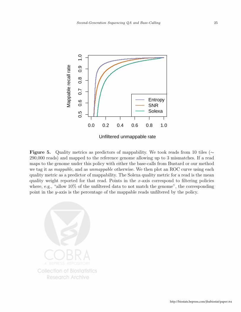
Figure 5 shows that the two metrics we have defined are significantly better predictors

of read mappability than the quality values provided by the manufacturer. The plot was



created as follows: we mapped 10 tiles of data (∼ 290,000 reads) allowing for a maximum of

3 mismatches anywhere on the read; if a read mapped under this policy (either by our, or

Solexa base-calls) it was labeled as mappable, and labeled as unmappable otherwise. We then

plot an ROC curve (Fawcett, 2004) using each quality metric as a predictor of mappability.

We see that both metrics outperform the manufacturer’s, with Entropy being the better of

the two. Again, this is not surprising, since Entropy is a function of the probability profiles,

which, due to the base-cycle effects, are not a simple function of the linear read-specific

models. One interpretation of this plot is that if a filtering policy is defined using an allowable

mismatch rate of 10%, then the Solexa metric will only recover 60% of the matching reads,

while SNR would recover 80%, and Entropy 90%.


6.3 Improved yield and accuracy

In this section we report on improved yield and accuracy resulting from using our model for

base-calling and quality assessment. We took the entire set of reads in our sample dataset

(one lane of data with ∼ 12 M 26 base-pair reads) and created files in the same format as

those produced by Solexa, consisting of a base-call and quality value for each base. We use

the Entropy metric as the quality value to each base, rescaled to the Phred (Ewing et al.,

1998) scale of quality values. This allows us to use existing mapping software, BOWTIE, in

this case, to map reads we produce to the genome. We also used Entropy to filter out reads

that have too many uncertain base-calls. Web Table W1 compares the mapping of our reads

to those produced by Solexa using the same mapping policy (at most two mismatches in the

first 24 positions). In summary, our base-caller yields an increase of more than 11% in the

number of reads mapped, and a 7% increase in the number of perfectly mapped reads. We

note that using the procedure discussed in the supplementary material, fitting our model for

base-calling takes roughly 1 minute per tile on a cluster node with a 3 GHz processor. Using



a 15 node cluster, we carried out the analysis of this full lane of data—both base-calling and

mapping with BOWTIE—in less than two hours.

6.4 Improved SNP calling

We processed the mapping from the previous Section using the MAQ SNP calling pipeline

to ascertain how our base-calling and quality metrics improves downstream analysis. Using

the Solexa pipeline, MAQ reported 37 high quality SNPs (Phred score > 100), while using

our base-calls and Entropy-based quality metric results in MAQ reporting only 10 SNPs,

a reduction of nearly 70% in false positives. As illustration, we replot Figure 2 using our

basecalls in Figure 6. While there is still some of the bias towards T in the tail of reads, it

is much less pronounced, enough for MAQ to avoid falsely calling this position a SNP.


7. Discussion

In this paper, we have presented some of the statistical and computational challenges pre-

sented by the analysis of second-generation sequencing data. In particular, we have shown

how infrequent but systematic errors arise in these data and how it can mislead downstream

analysis. In addition, the large variation in sequencing read quality must be captured in

meaningful and informative metrics and used judiciously in downstream analysis.

We have presented a model-based approach for quality assurance and base-calling of

data from the Illumina/Solexa second-generation sequencing platform that addresses these

shortcomings. Using a probabilistic model that properly captures technical features of the

raw continuous intensity data, yields simple but informative quality metrics. Furthermore,

it draws information across reads and sequencing cycles, and is able to quantify the global

variability inherent in the base-calling procedure. We have shown that our base-calling model

can improve on the manufacturer’s method in both yield and accuracy, leading to improved



genotyping down-stream analysis. The model attempts to capture effects in the intensity

data, in particular, read-cycle and base-cycle effects that lead to the technical biases we have

observed. While improvement is seen, there is still room for further improvement— better

capturing the base-cycle effect being the most immediate. We currently add a shift in the

intensity distribution according to base and cycle. However, these distributions vary beyond

shifts implying that a global strategy to model this variation might be required. We are

investigating further normalization strategies to address this (Bolstad et al., 2003).

Beyond improved performance, the model allows for easily interpretable metrics. In sit-

uations where there is a deluge of measurements to contend with, models that strive for

simplicity and interpretability are paramount. In addition, we implement a very efficient

method for parameter estimation that allows for analysis to be performed in hours rather

than weeks. Again, these types of concessions are required in data-intensive situations like

this one.

Our ultimate motivation for this work is to allow downstream analysis in clinical and

biological research using second-generation sequencing that appropriately quantifies and

captures the uncertainty inherent in the sequencing process. Along with collaborators, we

are applying our methods in multiple projects. One example is microRNA profiling and

discovery (Morin et al., 2008). In this case, the DNA fragments to sequence are short and

require that DNA strands, called adapters, be attached to each fragment of interest. An initial

step in analysis is finding this adapter within each resulting read, which can start at any

position along the read. Furthermore, the discovery of mutations in microRNA experiments

have attracted recent interest. We are developing a probabilistic framework that uses our

nucleotide probability profiles to incorporate robust adapter finding and variant discovery.

Another application of interest is variant discovery in pooled samples, where the frequency



of true genetic variants is close to the biased error rates we discussed above. Again, our

methods allow for a sound framework in which to carry out this type of analysis.

Supplementary Materials

Web Appendices and Figures referenced are available under the Paper Information link at

the Biometrics website http://www.biometrics.tibs.org. Source code implementing our

methodology can be found at http://www.biostat.jhsph.edu/~hcorrada/secgen.

Acknowledgements

This research was funded in part by ###.

References

Bennett, S. T., Barnes, C., Cox, A., Davies, L., and Brown, C. (2005). Toward the 1,000

dollars human genome. Pharmacogenomics 6, 373–82.

Bolstad, B. M., Irizarry, R. A., Astrand, M., and Speed, T. P. (2003). A comparison of

normalization methods for high density oligonucleotide array data based on variance

and bias. Bioinformatics 19, 185–193.

Dempster, A., Laird, N., and Rubin. . . , D. (1977). Maximum likelihood from incomplete

data via the em algorithm. Journal of the Royal Statistical Society .

Dohm, J. C., Lottaz, C., Borodina, T., and Himmelbauer, H. (2008). Substantial biases in

ultra-short read data sets from high-throughput dna sequencing. Nucleic Acids Res 36,

e105.

Erlich, Y., Mitra, P. P., delaBastide, M., McCombie, W. R., and Hannon, G. J. (2008).

Alta-cyclic: a self-optimizing base caller for next-generation sequencing. Nat Methods 5,

679–82.



Ewing, B., Hillier, L., Wendl, M. C., and Green, P. (1998). Base-calling of automated

sequencer traces using phred. i. accuracy assessment. Genome Res 8, 175–85.

Fawcett, T. (2004). ROC graphs: Notes and practical considerations for researchers. Machine

Learning 31,.

Hayden, E. C. (2008). International genome project launched. Nature 451, 378–9.

Ji, H., Jiang, H., Ma, W., Johnson, D. S., Myers, R. M., and Wong, W. H. (2008). An

integrated software system for analyzing chip-chip and chip-seq data. Nat Biotechnol

26, 1293–300.

Jothi, R., Cuddapah, S., Barski, A., Cui, K., and Zhao, K. (2008). Genome-wide identification

of in vivo protein-dna binding sites from chip-seq data. Nucleic Acids Res 36, 5221–31.

Langmead, B., Trapnell, C., Pop, M., and Salzberg, S. (2009). Ultrafast and memory-efficient

alignment of short dna sequences to the human genome. Genome Biology To appear.

Ledford, H. (2008). The death of microarrays? Nature 455, 847.

Li, H., Ruan, J., and Durbin, R. (2008). Mapping short dna sequencing reads and calling

variants using mapping quality scores. Genome Research .

Li, L. and Speed, T. P. (1999). An estimate of the crosstalk matrix in four-dye fluorescence-

based dna sequencing. Electrophoresis 20, 1433–42.

Margulies, M., Egholm, M., Altman, W. E., and et al. (2005). Genome sequencing in

microfabricated high-density picolitre reactors. Nature 437, 376–80.

Marioni, J. C., Mason, C. E., Mane, S. M., Stephens, M., and Gilad, Y. (2008). Rna-seq:

an assessment of technical reproducibility and comparison with gene expression arrays.

Genome Res 18, 1509–17.

Mikkelsen, T. S., Ku, M., Jaffe, D. B., Issac, B., Lieberman, E., Giannoukos, G., Alvarez,

P., Brockman, W., Kim, T.-K., Koche, R. P., Lee, W., Mendenhall, E., O’Donovan, A.,

Presser, A., Russ, C., Xie, X., Meissner, A., Wernig, M., Jaenisch, R., Nusbaum, C.,



Lander, E. S., and Bernstein, B. E. (2007). Genome-wide maps of chromatin state in

pluripotent and lineage-committed cells. Nature 448, 553–60.

Morin, R. D., O’Connor, M. D., Griffith, M., Kuchenbauer, F., Delaney, A., Prabhu, A.-L.,

Zhao, Y., McDonald, H., Zeng, T., Hirst, M., Eaves, C. J., and Marra, M. A. (2008).

Application of massively parallel sequencing to microrna profiling and discovery in human

embryonic stem cells. Genome Res 18, 610–21.

Mortazavi, A., Williams, B. A., McCue, K., Schaeffer, L., and Wold, B. (2008). Mapping

and quantifying mammalian transcriptomes by rna-seq. Nat Methods 5, 621–8.

Rougemont, J., Amzallag, A., Iseli, C., Farinelli, L., Xenarios, I., and Naef, F. (2008).

Probabilistic base calling of solexa sequencing data. BMC Bioinformatics 9,.

Shendure, J., Porreca, G. J., Reppas, N. B., Lin, X., McCutcheon, J. P., Rosenbaum, A. M.,

Wang, M. D., Zhang, K., Mitra, R. D., and Church, G. M. (2005). Accurate multiplex

polony sequencing of an evolved bacterial genome. Science 309, 1728–32.

Valouev, A., Johnson, D. S., Sundquist, A., Medina, C., Anton, E., Batzoglou, S., Myers,

R. M., and Sidow, A. (2008). Genome-wide analysis of transcription factor binding sites

based on chip-seq data. Nat Methods 5, 829–34.

Zhang, Y., Liu, T., Meyer, C. A., Eeckhoute, J., Johnson, D. S., Bernstein, B. E., Nussbaum,

C., Myers, R. M., Brown, M., Li, W., and Liu, X. S. (2008). Model-based analysis of

chip-seq (macs). Genome Biol 9, R137.

Received April 2009. Revised September 2009.



0 10 20 30 40

0.00

0.02

0.04

0.06

0.08

0.10

Manufacturer’s weight

Err

or r

ate

0 5 10 15 20 25 30 35

0.00

0.02

0.04

0.06

0.08

0.10

Sequencing cycleE

rror

rat

e(a) Left pane: We plot the estimated error rate for each quality weight level reported by themanufacturer. Right pane: We plot the estimated error rate for each sequencing cycle.

0 5 10 15 20 25 30 35

0.00

0.02

0.04

0.06

0.08

Sequencing cycle

Err

or r

ate

T−AC−AG−AA−TC−TG−TA−CT−CG−CA−GT−GC−G

(b) Proportion of specific base substitution errors. Label T-A indicates that at amismatching position, the reference genome has a T, while the aligned read has A.

Figure 1. Exploration of sequencing errors. The top two plots show how the quality weightreported by the manufacturer is not a very good predictor of errors compared to sequencingcycle. We see also that the number of errors increases considerably as sequencing cyclesprogress. The bottom plot shows that certain erroneous base substitutions are more prevalentthat others, that is, there is technical bias in sequencing errors. We see later how thesetechnical biases influence downstream analysis.



Sequencing cycle

Nuc

leot

ide

com

posi

tion

0.0

0.2

0.4

0.6

0.8

1.0

0 10 20 30

A

T

Figure 2. We plot the base composition of reads aligning to a specific genomic positionfalsely reported by MAQ as a SNP. We stratify base composition by cycle, that is, at tick1 of the x-axis we plot the base composition of the first cycle in reads which align to theSNP site in the first cycle, and so on. We can see a trend whereupon T’s become much morefrequent only in reads that align to the SNP site at later sequencing cycles, indicating atechnical bias in base-calls at this position.



Sequencing cycle

h(in

tens

ity)

11

12

13

14

0 10 20 30 0 10 20 30 0 10 20 30

11

12

13

14

11

12

13

14

0 10 20 30 0 10 20 30

11

12

13

14

Figure 3. The read-cycle effect. Each panel corresponds to measured intensities for a singleread. The upper (blue) points are the maximum intensity at each sequencing cycle, the lower(pink) points are the median of the remaining intensities. We can observe the cycle effect:signal (upper line) drops and background (lower line) rises. Observe that due to the startedlog transform, using a linear model for this effect is appropriate. The intercept of the signalmodel (upper line) captures the read effect, while the slope captures the cycle effect, andsimilarly for the background model (lower line).



SNR

Den

sity

0 500000

Entropy

Den

sity

0 20 40 60

cycle

14.6

14.8

15.0

15.2

15.4

cycle

14.7

14.8

14.9

15.0

15.1

15.2

Figure 4. Four read quality metrics. The first plot in each row gives a histogram of themetric for a sample of reads. The plots that follow in each row give exemplary data fromreads across the quality metric spectrum. The leftmost is a read with very low metric value,the rightmost is a read with a very high value, the two middle reads have close to medianquality metric values.



Unfiltered unmappable rate

Map

pabl

e re

call

rate

0.0 0.2 0.4 0.6 0.8 1.0

0.5

0.6

0.7

0.8

0.9

1.0

EntropySNRSolexa

Figure 5. Quality metrics as predictors of mappability. We took reads from 10 tiles (∼290,000 reads) and mapped to the reference genome allowing up to 3 mismatches. If a readmaps to the genome under this policy with either the base-calls from Bustard or our methodwe tag it as mappable, and as unmappable otherwise. We then plot an ROC curve using eachquality metric as a predictor of mappability. The Solexa quality metric for a read is the meanquality weight reported for that read. Points in the x-axis correspond to filtering policieswhere, e.g., “allow 10% of the unfiltered data to not match the genome”, the correspondingpoint in the y-axis is the percentage of the mappable reads unfiltered by the policy.



Sequencing cycle

Nuc

leot

ide

com

posi

tion

0.0

0.2

0.4

0.6

0.8

1.0

0 10 20 30

A

T

Figure 6. We redo Figure 2 using our own base-calls. Notice the reduced bias in T calls atthe tail of reads aligning to the SNP position. MAQ does not report this position as a SNPusing our base-calls.


Web-based Supplementary Materials for Model-Based Quality

Assessment and Base-Calling for

Second-Generation Sequencing Data

Hector Corrada Bravo Rafael A. IrizarryJohns Hopkins Biostatistics, MD 21206, USA

September 8, 2009

1 Exploratory data analysis plots

0 2000 4000 6000 8000

050

0010

000

0.5(A+T)

A−

T

cycle < 20cycle ≥ 20

Figure W1: Comparative plot of measured intensities for the A and T channels for reads aligned to thereported SNP site of Figure 2. Points above the blue line result in A base calls. We see that T calls come

from measurements that are not very clear and the majority occur after sequencing cycle 20.

1


Four−channel fluorescence intensity

A

C

G

T

: cycle 1

A

C

G

T

: cycle 15

A

C

G

T

: cycle 25

A

C

G

T

: cycle 35

ACGTN

Figure W2: Fluorescence intensity data. Each panel of this figure corresponds to a sequencing cycle j =

1, 15, 25, 35. Within each panel, we plot the intensities of two channels, e.g. the top left panel of each plot

shows YijA vs. YijT . Points are color coded according to the base-call made by the Illumina/Solexa Bustardbase-caller.

2


read

h(in

tens

ity)

11.0

11.5

12.0

12.5

13.0

13.5

14.0

Figure W3: The read effect makes overall intensity measurements from each read vary across reads. Each

boxplot contains the 4N (N = 36) transformed intensity measurements of a single read. We have orderedthe boxplots by increasing median to clearly illustrate the large range in which overall measured intensity

varies.

base

h(m

ax in

tens

ity)

11

12

13

14

: cycle 1 : cycle 5 : cycle 10

: cycle 15 : cycle 20

11

12

13

14

: cycle 24

11

12

13

14

A C G T

: cycle 28

A C G T

: cycle 32

A C G T

: cycle 35

Figure W4: The base-cycle effect shows how the distribution of intensities in the high range changes differ-

ently for each base. In this case we only plot the maximum intensity of each read-cycle in the boxplot for

the appropriate channel.

3


2 Model parameter estimation

Our procedure to estimate the model parameters in Eq. (1) is based on the EM framework [1], that is, it maybe understood as an iterative procedure that treats the estimation problem as a missing data problem, where

each iteration computes model estimates conditioned on the expected value of the unobserved data, in our

case, the nucleotide probability profiles zijc. However, since our setting requires estimating a large numberof parameters we do not compute maximum likelihood estimates since we make two changes to the proper

M-step for computational considerations. In this Section we completely specify our estimation procedure.

First, we give maximum likelihood estimates in a slightly simplified setting so that the modifications wemake to our procedure for the full model are clearly identified.

Preliminaries Consider the following model:

yij = Xai + bj + ǫij ,

where yij is a real-valued outcome, ai ∈ Rp, i = 1, . . . , n, j = 1, . . . , m and ǫij is an error term with

ǫij ∼ N(0, σ2

i ). For identifiability we require parameters to satisfy the constraint XT b = 0, where b is the

vector of parameters bj . In our full model, read-specific parameters αi or βi will take the place of ai in

this setting, while base-cycle effect parameters µcjα or µcjβ will take place of bj . The log-likelihood of thesemodel parameters given a set of observations yij is

l(µ, a, σ2; y) = −nm

2−

m

2

∑

i

log σ2

i −1

2

∑

i

1

σ2

i

(yi − Xai − b)T (yi − Xai − b),

where yi ∈ Rm is the vector of observations yij with index i.

The gradient of the likelihood with respect to parameter ai is

∇ail =

1

2σ2

i

XT (yi − Xai − b),

Setting to zero, assuming X is of full-column rank (which it is in our case), and due to the identifiability

constraint XT b = 0, we get that the MLE of ai is given by

ai = (XT X)−1XT yi.

On the other hand, the gradient of the likelihood with respect to parameter b is given by

∇bl =1

2

∑

i

s2

i (yi − Xai − b),

where s2

i = 1

σ2

i

. Setting to zero, and plugging in the MLE for ai, we get that the MLE of b satisfies

b =∑

i

s2

i

s2(yi − Xai),

where s2 =∑

i s2

i . We can check the MLE satisfies the identifiability constraint:

XT b = XT

[

∑

i

s2

i

s2(yi − Xai)

]

=∑

i

s2

i

s2

[

XT yi − XT X(XT X)−1XT yi

]

= 0.

Therefore, the MLE of b, under identifiability constraint XT b = 0, is a weighted average of residual vectors

ri := yi − Xai with weights determined by variances σ2

i .

Finally, the derivative of the likelihood with respect to parameter σ2

i is:

∂l

∂σ2

i

= −m

2σ2

i

+1

2(σ2

i )2(yi − Xai − b)T (yi − Xai − b),

4


which setting to zero gives that the MLE of σ2

i satisfies

σ2

i =1

m(yi − Xai − b)T (yi − Xai − b).

This gives the MLE estimates under this simplified setting, which will help us identify the modifications wemake to our procedure for computational considerations which make our estimates deviate from the MLEs.

Model estimates The intensity model is defined in Equation 1 in Section 4 of the main paper as:

uijc = ∆ijc

[

µcjα + α0i + (j − 1)α1i + ǫαijc

]

+ (1 − ∆ijc)[

µcjβ + β0i + (j − 1)β1i + ǫβijc

]

, (1)

where ǫαijc ∼ N(0, σ2

αi) and ǫβijc ∼ N(0, σ2

βi) for all i, j, c, and ∆ijc is an indicator of the underlying,unobserved, nucleotide being sequenced for read i in cycle j. That is,

∆ijc =

{

1 if c is the nucleotide in read i position j

0 otherwise,

and∑

c ∆ijc = 1 for all i, j. The log likelihood of the model parameters conditioned on the unobserved ∆i

given the measured intensities (ui) is:

l0(θ; ui, ∆i) =

N∑

j=1

∑

c

I{∆ijc = 1} log fθc(uij)

+∑

j

∑

c

I{∆ijc = 1} logπc,

where πc is the marginal probability of observing nucleotide c, and

fθc(uij) = ϕσ2

αi(uijc − µcjα − α0i − (j − 1)α1i) ×

∏

k 6=c

ϕσ2

βi(uijk − µkjβ − β0i − (j − 1)β1i) ,

with ϕσ2(·) the density function of the N(0, σ2) distribution. As above, we impose the constraints XT µcα = 0

and XT µcβ for identifiability, where vector Xj = [1 (j − 1)] and µcα and µcβ are the vectors of base-cycleeffects for base c, µcjα and µcjβ respectively.

We now give our procedure for deriving estimates for model parameters based on the EM-framework:

E-step Given current estimates π and θ, the E-step computes zijc = E{∆ijc = 1} as

zijc =πcfθc(uij)

∑

k πkfθk(uij), (2)

M-step We introduce one last bit of notation: Zic is a diagonal matrix with jth entry zijc, and uic isthe vector of observations for read i along channel (nucleotide) c. Also, observe that

∑

c Zic = I and∑

c(I −Zic) = 3I. Given current estimate zijc, the other parameters are estimated as follows. The gradientwith respect to parameter αi is given by

∇αiQ =

1

2σ2

αi

XT

[

∑

c

Zic(uic − Xαi − µcα)

]

. (3)

Setting to zero, and assuming X is of full column rank, we have that due to the identifiability constraint

and the property of Zic given above, we can estimate αi as:

αi = (XT X)−1XT uαi,

5


where uαi =∑

c Zicuic. Similarly, we can estimate βi as

βi =1

3(XT X)−1XT uβi,

where uβi =∑

c(I − Zic)uic.

Estimating αi and βi then entails solving two small weighted least squares problems. However, as seenabove, the weight matrix sums to identity, so the matrix on the left-hand side of the normal equations is

unchanged for all Zic. Thus, a single Cholesky decomposition is required to solve all problems across all

reads over all iterations of the algorithm. This makes our procedure extremely computationally efficientsince we compute this decomposition once and re-use it for all reads and iterations.

The gradient with respect to parameter µcα is given by

1

2

∑

ic

1

σ2

αi

Zic(uic − Xαi − µcα).

Setting to zero, we get that the maximizer satisfies

µcα =∑

i

s2

αi

s2α

Zic(uic − Xαi),

where as before s2

αi = 1

σ2

i

and s2

α =∑

αi s2

i . As above, we observe that the MLE of µcα is a weighted average,

but in this case, the weight is given by both variance σ2

i and the current estimate of the posteriors zijc. Here

we make our first deviation from MLEs: we use only posteriors zijc as weights by setting s2

αi/s2

α = 1/Mfor all i. This then decouples the estimation of the base-cycle parameters µcα and the variance parameters

σ2

αi, which makes our procedure computationally tractable (see main paper for a discussion on the number

of parameters to estimate). Using this decoupling, we have

µcjα =1

M

∑

i

zijc(uijc − α0i − (j − 1)α1i).

Our final modification is motivated by wanting to make these estimates robust: µcjα is estimated as the

median of the weighted residuals zijc(uijc − α0i − (j − 1)α1i) instead. Similarly, µcjβ is estimated as the

median of the weighted residuals (1 − zijc)(uijc − β0i − (j − 1)β1i).Finally, once parameters αi, βi, µcjα and µcjβ are estimated for all i, j, c as above, we estimate variance

parameters by:

σ2

αi =1

N

∑

jc

zijc (yijc − α0i − (j − 1)α1i − µcjα)2 ,

and

σ2

βi =1

3N

∑

jc

(1 − zijc) (yijc − β0i − (j − 1)β1i − µcjβ)2.

Marginal probabilities π can be fixed to nucleotide proportions in a reference genome, or estimated as:

πc =1

NM

∑

i,j

zijc (4)

Initialization To conclude, we specify how to initialize our algorithm. Given observations u, parameters

are initialized as πc = 1/4; αi1 = βi1 = 0; αi0 = Q5/6

jc (uijc) and βi0 = Q1/2

jc (uijc), where Qq is the q-th

quantile function; µcjα = µcjβ = 0; σ2

αi = 1

|Ri|

∑

ijc r2

ijc where Ri = {uijc|uijc >= Q2/3

j′c′(uij′c′)} and

rijc =

{

uijc − α0i if uijc ∈ Ri

0 o.w.,

6


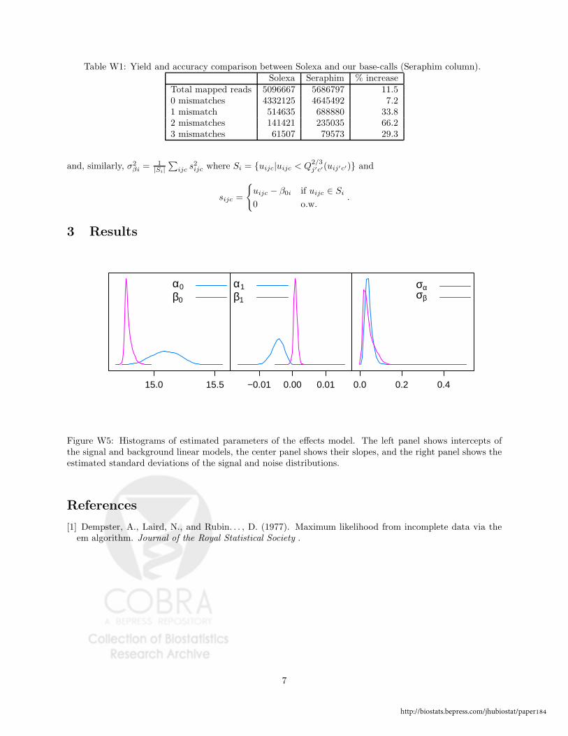
Table W1: Yield and accuracy comparison between Solexa and our base-calls (Seraphim column).

Solexa Seraphim % increase

Total mapped reads 5096667 5686797 11.5

0 mismatches 4332125 4645492 7.2

1 mismatch 514635 688880 33.82 mismatches 141421 235035 66.2

3 mismatches 61507 79573 29.3

and, similarly, σ2

βi = 1

|Si|

∑

ijc s2

ijc where Si = {uijc|uijc < Q2/3

j′c′(uij′c′)} and

sijc =

{

uijc − β0i if uijc ∈ Si

0 o.w..

3 Results

15.0 15.5

α0

β0

−0.01 0.00 0.01

α1

β1

0.0 0.2 0.4

σασβ

Figure W5: Histograms of estimated parameters of the effects model. The left panel shows intercepts of

the signal and background linear models, the center panel shows their slopes, and the right panel shows the

estimated standard deviations of the signal and noise distributions.

References

[1] Dempster, A., Laird, N., and Rubin. . . , D. (1977). Maximum likelihood from incomplete data via theem algorithm. Journal of the Royal Statistical Society .

7


cycle

−0.03

0

0.03

0 10 20 30

A

AAAAAAAAAAAAAAAAAAAAAAAAAAAAAAAAAA

A

C

CCCCCCCCCCCCCCCCCCCCCCCCCCCCCCCCC

CC

G

GGGGGGGGGG

GGGGGGGGGGGGGGGGGGGGGG

GGGT

TTTTTTTTTT

TTTTTTTTTTTTTTT

TTTTTTTTTT

A

AAAAAAAAA

AAAAAAAAAAAAAAAAAAAAAAAA

AA

C

CCCCCCCCC

CCCCCCCCCCCCCCCCCCCCCCCCC

C

G

GGG

GGGGGG

GGGGGGGGGGGGGGGGGGGGGGG

GGG

T

TTTTTTTTT

TTTTTTTT

TTTT

TTTTTTTTT

TTTTT

0 10 20 30

A

AAAAAAAAAA

AAAAAAAAAAAAAAAAAAAAA

AAAA

C

CCCCCCCCCCCCCCCCCCCCCCCCCCCCCCCCCCC

G

GGGGG

GGGG

GGGGGGGGGGGGGG

GGGGGGGGGGGGT

TTTT

TTTTTT

TTTTTTTTTTT

TTTT

TTTTTTT

TTT

AAAAAAAAAAAAAAAAAAAAAAAAAAAAAAAAAAAACCCCCCCCC

CCCCCCCCCCCCCCCCCCCCCCCCCCCGGGGGGGGGGGGGGGGGGGGGGGGGGGGGGGGGGG

GTTTTTTTTTTTTTTTTTTTT

TTTTTTTTTTTTTTT

T

0 10 20 30

AAAAAAAAAAAAAAAAAAAAAAAAAAAAAAAAAAA

ACCCCCCCCCCCCCCCCCCCCCCCCCCCCCCCCCCC

CGGGGGGGGGGGGGGGG

GGGGGGGGGGGGGGGGGGGGTTT

TTTTTTTTTTTTTTT

TTTTTTTTTTTTTTTTT

T

−0.03

0

0.03

AAAAAAAAAAAAAAAAAAAAAAAAAAAAAAAAAAA

ACCCC

CCCCCCCCCCCCCCCCCCCCCCCCCCCCCCC

C

GGGGGGGGGGGGGGGGGGGGGGGGGGGGGGGGGGG

GTTTTTTTTTTTTTTTTTT

TTTTTTTTTTT

TTTTTT

T

Figure W6: Estimated base-cycle effects for three sets of reads. Notice an overall adjustment of T intensitiesdownward, which increases in later sequencing cycles. The upper row shows estimates for the base-cycle

effect of the background model µcjβ , while the lower row shows estimates for the signal model µcjα.

8


Documents

MODEL-BASED QUALITY ASSESSMENT AND BASE-CALLING FOR …