Embed Size (px)
Citation preview

Model-based Predictive Control for Improving
Stability and Transparency in Time-delay
Teleoperation

MODEL-BASED PREDICTIVE CONTROL FOR IMPROVING
STABILITY AND TRANSPARENCY IN TIME-DELAY
TELEOPERATION
BY
ALI SHAHDI, M.A.Sc., (Electrical Engineering)
McMaster University, Hamilton, Canada
A THESIS
SUBMITTED TO THE DEPARTMENT OF ELECTRICAL & COMPUTER ENGINEERING
AND THE SCHOOL OF GRADUATE STUDIES
OF MCMASTER UNIVERSITY
IN PARTIAL FULFILMENT OF THE REQUIREMENTS
FOR THE DEGREE OF
DOCTOR OF PHILOSOPHY
c© Copyright by Ali Shahdi, April 2010
All Rights Reserved

Doctor of Philosophy (2010) McMaster University
(Electrical & Computer Engineering) Hamilton, Ontario, Canada
TITLE: Model-based Predictive Control for Improving Stabil-
ity and Transparency in Time-delay Teleoperation
AUTHOR: Ali Shahdi
M.A.Sc., (Electrical Engineering)
McMaster University, Hamilton, Canada
B.Sc., (Electrical Engineering)
Sharif University of Technology, Tehran, Iran
SUPERVISOR: Dr. Shahin Sirouspour
NUMBER OF PAGES: xv, 246
ii

To My Parents

Acknowledgements
I owe my deepest gratitude to my supervisor, Dr. Shahin Sirouspour, for his end-
less support, guidance and encouragement. I want to thank him for his deep in-
sight, broad knowledge and tremendous effort during all the stages of the pro-
gram.
I am indebted to my colleagues at Telerobotics, Haptics, and Computational
Vision Lab, for their kind helps and friendship. I would also like to thank my
friends for their support, friendship and reminding me that there is life beyond
school.
Last but not least, my sincere thanks go to my parents who always support
and encourage me through my life. Their understanding and patience have made
it possible to pass all the steps. Without their supports, completion of this thesis
would not have been possible.
iv

Abstract
Prior research on time-delay bilateral teleoperation has mainly resulted in meth-
ods that favor the robust stability of the system at the expense of its transparency.
In contrast, it is demonstrated in this thesis that carefully designed model-based
predictive controllers are able to achieve high levels of transparency while main-
taining teleoperation stability. This is accomplished by utilizing available informa-
tion on system model and time delay within a predictive control framework. The
performance objectives are delay-free position tracking between the master and
slave and the establishment of a virtual mass-damper tool impedance between the
user and environment. Three model-based predictive controllers are proposed in
this thesis which utilize both force and position measurements at the master and
slave sites. The first two controllers can only handle known and fixed time delays
whereas the third controller is applicable to systems with fixed or variable delay.
First, building upon our recent work in [1, 2], a decentralized model-based
predictive controller is introduced that can enhance the time-delay teleoperation
transparency and robust stability by allowing the use of local delay-free measure-
ments in local master/slave controllers. The stability of the system is analyzed
using a frequency sweeping test. Numerical analysis demonstrates improved per-
formance and robustness compared with the centralized controller in [2].
v

Next, a robust predictive controller is proposed to deal with modeling uncer-
tainty, particularly in the operator and environment dynamics. In a two-step con-
trol approach, first local adaptive/nonlinear controllers are applied to linearize the
system dynamics and to eliminate dependency on the master and slave parame-
ters. Teleoperation coordination is then achieved by formulating an input/output
(I/O) time-delay H∞ robust control synthesis. The transparency and robust stabil-
ity properties of the proposed method are examined via numerical analysis.
Although less sensitive to modeling uncertainty, the robust controller can still
sacrifice teleoperation transparency in favor of its stability since it utilizes a fixed
controller for the entire range of teleoperation. In an attempt to avoid such a trade-
off, a stable adaptive predictive controller for teleoperation systems with constant
and varying communication delay is proposed. The controller utilizes a model of
the system dynamics and the time delay within a predictive control framework to
achieve the desired transparency objectives while maintaining the system stabil-
ity. The controller adapts to uncertainties in the system dynamics by estimating
the model parameters in real time. A Lyapunov analysis of the performance and
stability of the resulting system is presented.
The proposed controllers for time-delay bilateral teleoperation are implemented
and experimentally evaluated. The results demonstrate the effectiveness of the
proposed methods in providing a stable transparent interface for teleoperation un-
der time delay.
vi

Contents
Acknowledgements iv
Abstract v
1 Introduction and Problem Statement 1
1.1 Background . . . . . . . . . . . . . . . . . . . . . . . . . . . . . . . . . 1
1.2 Motivation . . . . . . . . . . . . . . . . . . . . . . . . . . . . . . . . . . 3
1.3 Summary of Thesis Contributions . . . . . . . . . . . . . . . . . . . . 6
1.4 Organization of the Thesis . . . . . . . . . . . . . . . . . . . . . . . . . 12
1.5 Related Publications . . . . . . . . . . . . . . . . . . . . . . . . . . . . 13
1.5.1 Journal Articles . . . . . . . . . . . . . . . . . . . . . . . . . . . 13
1.5.2 Conference Papers . . . . . . . . . . . . . . . . . . . . . . . . . 13
2 Literature Review 15
2.1 Introduction . . . . . . . . . . . . . . . . . . . . . . . . . . . . . . . . . 15
2.2 Teleoperation Control Architectures . . . . . . . . . . . . . . . . . . . 16
2.3 Control of Delay-free Teleoperation . . . . . . . . . . . . . . . . . . . . 17
2.3.1 Robust Controllers . . . . . . . . . . . . . . . . . . . . . . . . . 21
2.3.2 Adaptive Controllers . . . . . . . . . . . . . . . . . . . . . . . . 22
vii
2.4 Time-delay Teleoperation Control . . . . . . . . . . . . . . . . . . . . . 24
2.4.1 Passivity-based Controllers . . . . . . . . . . . . . . . . . . . . 25
2.4.2 Robust Controllers . . . . . . . . . . . . . . . . . . . . . . . . . 28
2.4.3 Predictive Controllers . . . . . . . . . . . . . . . . . . . . . . . 29
2.5 Time-delay Systems . . . . . . . . . . . . . . . . . . . . . . . . . . . . . 30
3 Teleoperation Dynamics and Performance Objectives 34
3.1 Introduction . . . . . . . . . . . . . . . . . . . . . . . . . . . . . . . . . 34
3.2 Robot Dynamics . . . . . . . . . . . . . . . . . . . . . . . . . . . . . . . 35
3.3 Teleoperation System Dynamics . . . . . . . . . . . . . . . . . . . . . . 39
3.4 Performance of Master/Slave Teleoperation Systems . . . . . . . . . 42
4 Model-based Decentralized Control of Time-delay Teleoperation Systems 46
4.1 Introduction . . . . . . . . . . . . . . . . . . . . . . . . . . . . . . . . . 46
4.2 Linearization of Master/Slave Teleoperation Systems Dynamics . . . 48
4.3 Decentralized Time-delay Teleoperation System . . . . . . . . . . . . 55
4.3.1 Free motion/soft contact . . . . . . . . . . . . . . . . . . . . . . 59
4.3.2 Rigid contact . . . . . . . . . . . . . . . . . . . . . . . . . . . . 62
4.4 Reduction and Control of Time-delay Systems . . . . . . . . . . . . . 65
4.4.1 Closed-loop Stability Analysis . . . . . . . . . . . . . . . . . . 72
4.5 Performance and Robust Stability Analysis for Single-axis Teleoper-
ation . . . . . . . . . . . . . . . . . . . . . . . . . . . . . . . . . . . . . 77
4.5.1 Robust stability analysis w.r.t parametric uncertainty . . . . . 79
4.5.2 Performance analysis . . . . . . . . . . . . . . . . . . . . . . . . 81
viii
4.5.3 Robust stability analysis w.r.t. perturbations in communica-
tion delay . . . . . . . . . . . . . . . . . . . . . . . . . . . . . . 82
4.6 Experimental Results . . . . . . . . . . . . . . . . . . . . . . . . . . . . 86
4.6.1 Decentralized controller with 100 ms delay . . . . . . . . . . . 88
4.6.2 Decentralized controller with 200 ms delay . . . . . . . . . . . 89
4.6.3 Decentralized controller with 300 ms delay . . . . . . . . . . . 90
4.7 Conclusions . . . . . . . . . . . . . . . . . . . . . . . . . . . . . . . . . 90
5 Adaptive/Robust Control for Time-delay Teleoperation 93
5.1 Introduction . . . . . . . . . . . . . . . . . . . . . . . . . . . . . . . . . 93
5.2 Master/Slave Local Adaptive Control . . . . . . . . . . . . . . . . . . 94
5.3 Teleoperation Control Formulation . . . . . . . . . . . . . . . . . . . . 99
5.4 H∞ Control of MIMO Systems with I/O time delay . . . . . . . . . . 107
5.4.1 Problem Formulation . . . . . . . . . . . . . . . . . . . . . . . 109
5.4.2 Equivalent One-block Problem . . . . . . . . . . . . . . . . . . 110
5.4.3 The Adobe Delay Problem . . . . . . . . . . . . . . . . . . . . . 112
5.4.4 Decomposition . . . . . . . . . . . . . . . . . . . . . . . . . . . 113
5.5 Design Example . . . . . . . . . . . . . . . . . . . . . . . . . . . . . . . 115
5.6 Experimental Results . . . . . . . . . . . . . . . . . . . . . . . . . . . . 127
5.6.1 Teleoperation experiment with 100 msec delay . . . . . . . . . 128
5.6.2 Teleoperation experiment with 200 msec delay . . . . . . . . . 130
5.6.3 Teleoperation experiment with 300 msec delay . . . . . . . . . 131
5.7 Conclusions . . . . . . . . . . . . . . . . . . . . . . . . . . . . . . . . . 131
6 Adaptive Control of Bilateral Time-delay Teleoperation 133
ix
6.1 Introduction . . . . . . . . . . . . . . . . . . . . . . . . . . . . . . . . . 133
6.2 Revised Time-delay Teleoperation System Formulation . . . . . . . . 134
6.3 Modified Delay Reduction and Model-based State Prediction . . . . . 137
6.4 New Outputs Definition and Regulation . . . . . . . . . . . . . . . . . 143
6.5 System Stability and Parameters Adaptation Law . . . . . . . . . . . 148
6.5.1 Output Regulation . . . . . . . . . . . . . . . . . . . . . . . . . 155
6.6 Parameter Convergence and Composite Adaptive Control . . . . . . 156
6.6.1 Composite Adaptive Control . . . . . . . . . . . . . . . . . . . 157
6.7 Adaptive Control of Teleoperation with Time-varying Delay . . . . . 162
6.7.1 Practical Implementation Issues for the Time-varying Con-
troller in Packet Switched Networks . . . . . . . . . . . . . . . 169
6.8 Experimental Results . . . . . . . . . . . . . . . . . . . . . . . . . . . . 171
6.8.1 Adaptive controller with 50 ms delay . . . . . . . . . . . . . . 173
6.8.2 Adaptive controller with 100 ms delay . . . . . . . . . . . . . . 175
6.8.3 Adaptive controller with 200 ms delay . . . . . . . . . . . . . . 176
6.8.4 Adaptive controller with time-varying delay . . . . . . . . . . 177
6.9 Conclusion . . . . . . . . . . . . . . . . . . . . . . . . . . . . . . . . . . 178
7 Conclusions and Future Work 180
7.1 Conclusions . . . . . . . . . . . . . . . . . . . . . . . . . . . . . . . . . 180
7.1.1 Model-based Decentralized Controller . . . . . . . . . . . . . . 181
7.1.2 Robust Controller . . . . . . . . . . . . . . . . . . . . . . . . . . 182
7.1.3 Adaptive Controller . . . . . . . . . . . . . . . . . . . . . . . . 183
7.2 Future Work . . . . . . . . . . . . . . . . . . . . . . . . . . . . . . . . . 184
x
A Master/Hand, Slave/Environment and Tool Dynamics in State-space Form187
B Teleoperation Dynamics in Chapter 4 in State-space Form 190
B.1 Free Motion/Soft Contact . . . . . . . . . . . . . . . . . . . . . . . . . 190
B.2 Rigid Contact . . . . . . . . . . . . . . . . . . . . . . . . . . . . . . . . 196
C Proof of Theorem 4.1 200
C.1 Stabilizability . . . . . . . . . . . . . . . . . . . . . . . . . . . . . . . . 200
C.2 Detectability . . . . . . . . . . . . . . . . . . . . . . . . . . . . . . . . . 205
D One-block Equivalent of a Four-block Time-delay Problem 209
E Solution to the Adobe Delay Problem 214
F Teleoperation Dynamics in Chapter 6 in State-space Form 217
F.1 Teleoperation Dynamics after Transformation . . . . . . . . . . . . . . 219
F.2 Teleoperation Dynamics in Chapter 6 in Closed-loop Form . . . . . . 222
F.3 Teleoperation Dynamics in Chapter 6 in Linear-in-parameter Form . 223
G The Persistency of Excitation Condition 225
H Composite Adaptive Controller Matrices 227
xi

List of Figures
1.1 (a) Unilateral teleoperation architecture with visual feedback and (b)
bilateral architecture with additional kinesthetic and force feedback. 2
2.1 A general bilateral teleoperation control architecture. . . . . . . . . . 16
2.2 Two-port network model of a teleoperation system. . . . . . . . . . . 17
3.1 Linear mass-spring-damper models of (a) the operator’s arm and (b)
the environment. . . . . . . . . . . . . . . . . . . . . . . . . . . . . . . 41
3.2 Operator and environment interaction through (a) ideally transpar-
ent teleoperation and (b) virtual intervening tool, with unity posi-
tion and force scaling factors. . . . . . . . . . . . . . . . . . . . . . . . 43
4.1 A centralized teleoperation architecture with controller at the mas-
ter site. . . . . . . . . . . . . . . . . . . . . . . . . . . . . . . . . . . . . 47
4.2 Conceptual representation of the proposed model-predictive decen-
tralized teleoperation controller: (a) Centralized teleoperation con-
trol at master or slave side; (b) Decentralized sub-controller design;
(c) Decentralized controller implementation. . . . . . . . . . . . . . . 57
4.3 Multi-model decentralized controller for time-delay teleoperation. . 75
4.4 Robust stability analysis results in free motion: (a), (b) and (c), and
in rigid contact: (d), as a function of time delay. . . . . . . . . . . . . . 80
xii

4.5 Robust stability analysis results in free motion: (b) and (c), and in
rigid contact: (a) and (d), for simultaneous variations in two param-
eters. . . . . . . . . . . . . . . . . . . . . . . . . . . . . . . . . . . . . . 81
4.6 ‖H‖22 for the closed-loop system from f ∗h to (a) position tracking er-
ror in free motion, (b) tool tracking error in free motion, (c) position
tracking error in rigid contact, and (d) force tracking error in rigid
contact. . . . . . . . . . . . . . . . . . . . . . . . . . . . . . . . . . . . . 83
4.7 Closed-loop decentralized teleoperation control subject to uncertainty
in communication delay. . . . . . . . . . . . . . . . . . . . . . . . . . . 84
4.8 Maximum/minimun allowable time-delay variations to maintain
stability. . . . . . . . . . . . . . . . . . . . . . . . . . . . . . . . . . . . . 85
4.9 The experimental setup. . . . . . . . . . . . . . . . . . . . . . . . . . . 87
4.10 Decentralized controller with 100 msec delay in experiment: (a) po-
sition tracking and (b) force tracking. . . . . . . . . . . . . . . . . . . . 89
4.11 Decentralized controller with 200 msec delay in experiment: (a) po-
sition tracking and (b) force tracking. . . . . . . . . . . . . . . . . . . . 90
4.12 Decentralized controller with 300 msec delay in experiment: (a) po-
sition tracking and (b) force tracking. . . . . . . . . . . . . . . . . . . . 91
5.1 Block diagram of master (slave) dynamics after the application of
local adaptive nonlinear controllers. . . . . . . . . . . . . . . . . . . . 98
5.2 Linearized teleoperation control system. . . . . . . . . . . . . . . . . . 101
5.3 A MIMO system with multiple I/O delays: (a) original; (b) after
applying the wave transformations. . . . . . . . . . . . . . . . . . . . 106
xiii
5.4 (a) Lower fractional transformation (LFT); (b) Scattering representa-
tion. . . . . . . . . . . . . . . . . . . . . . . . . . . . . . . . . . . . . . . 108
5.5 Equivalent one-block problem . . . . . . . . . . . . . . . . . . . . . . . 111
5.6 Controller reconstruction from a two-step adobe decomposition. . . . 119
5.7 Closed-loop frequency response to the input f ∗h for 100 msec delay
and matched environment stiffness. . . . . . . . . . . . . . . . . . . . 121
5.8 Closed-loop frequency response to the input f ∗h for 100 msec delay
and mismatched environment stiffness. . . . . . . . . . . . . . . . . . 121
5.9 Closed-loop frequency response to the input f ∗h for 200 msec delay
and matched environment stiffness. . . . . . . . . . . . . . . . . . . . 122
5.10 Closed-loop frequency response to the input f ∗h for 200 msec delay
and mismatched environment stiffness. . . . . . . . . . . . . . . . . . 122
5.11 Closed-loop frequency response to the input f ∗h for 300 msec delay
and matched environment stiffness. . . . . . . . . . . . . . . . . . . . 123
5.12 Closed-loop frequency response to the input f ∗h for 300 msec delay
and mismatched environment stiffness. . . . . . . . . . . . . . . . . . 123
5.13 The closed-loop system subject to the environment stiffness uncer-
tainty, δke. . . . . . . . . . . . . . . . . . . . . . . . . . . . . . . . . . . 124
5.14 Nyquist plot of R(s) for 100 msec of delay. . . . . . . . . . . . . . . . . 125
5.15 Nyquist plot of R(s) for 200 msec of delay. . . . . . . . . . . . . . . . . 126
5.16 Nyquist plot of R(s) for 300 msec of delay. . . . . . . . . . . . . . . . . 126
5.17 The two-stage teleoperation controller. . . . . . . . . . . . . . . . . . . 128
5.18 The controller with 100 ms delay in experiment: (a) position track-
ing; (b) force tracking; (c) estimated environment stiffness. . . . . . . 129
xiv

5.19 The controller with 200 ms delay in experiment: (a) position track-
ing; (b) force tracking; (c) estimated environment stiffness. . . . . . . 130
5.20 The controller with 300 ms delay in experiment: (a) position track-
ing; (b) force tracking; (c) estimated environment stiffness. . . . . . . 131
6.1 A centralized time-delay teleoperation control (a) without delay padding,
(b) after delay padding, (c) after combining master/operator and
slave/environment dynamics and (d) after moving all the delays to
the input channels. . . . . . . . . . . . . . . . . . . . . . . . . . . . . . 136
6.2 Communication over a packet switched network with (a) increasing
delay and (b) decreasing delay. . . . . . . . . . . . . . . . . . . . . . . 170
6.3 Control action and master/slave devices running with a faster sam-
pling rate than the communication packet transmission rate. . . . . . 171
6.4 Time-delay teleoperation system with the proposed adaptive pre-
dictive controller . . . . . . . . . . . . . . . . . . . . . . . . . . . . . . 172
6.5 Model-based adaptive controller with 50 msec delay in experiment:
(a) position tracking and (b) force tracking. . . . . . . . . . . . . . . . 174
6.6 Model-based adaptive controller with 100 msec delay in experiment:
(a) position tracking and (b) force tracking. . . . . . . . . . . . . . . . 175
6.7 Model-based adaptive controller with 200 msec delay in experiment:
(a) position tracking and (b) force tracking. . . . . . . . . . . . . . . . 176
6.8 The model-based adaptive controller with time-varying delay in (6.138):
(a) position tracking and (b) force tracking. . . . . . . . . . . . . . . . 178
6.9 The model-based adaptive controller with time-varying delay in (6.139):
(a) position tracking and (b) force tracking. . . . . . . . . . . . . . . . 179
xv

Chapter 1
Introduction and Problem Statement
1.1 Background
Operator-in-the-loop control of robotic manipulators, widely known as teleoper-
ation, has been an alternative to autonomous robotic operation in complex and
unstructured environments. Teleoperation systems allow a human operator to ex-
tend his/her intelligence and manipulation skills to remote and/or hazardous en-
vironments. This is achieved through coordinated control of two robotic arms, i.e.
a master hand-controller which is often a force-feedback enabled interface used
by the operator, and a slave robot that manipulates the task environment. The
coordination is carried out by master/slave controllers and by utilizing the posi-
tion and force information exchanged over the linking communication medium.
Figure 1.1 shows these six elements that usually constitute a teleoperation system.
After its initial introduction in 1940s, telerobotics has rapidly progressed from
mechanically linked tele-manipulation to current advanced computer-controlled
1
Ph.D. Thesis - A. Shahdi McMaster - Electrical Engineering
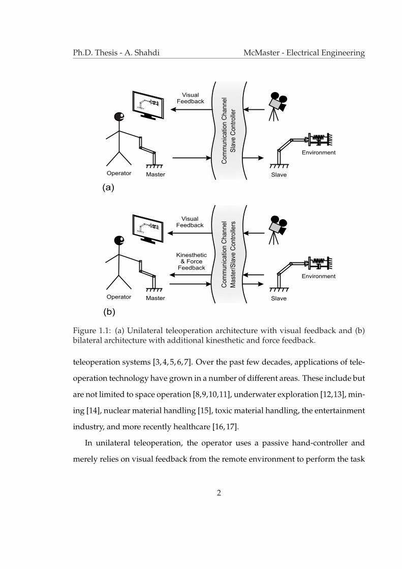
Figure 1.1: (a) Unilateral teleoperation architecture with visual feedback and (b)bilateral architecture with additional kinesthetic and force feedback.
teleoperation systems [3, 4, 5, 6, 7]. Over the past few decades, applications of tele-
operation technology have grown in a number of different areas. These include but
are not limited to space operation [8,9,10,11], underwater exploration [12,13], min-
ing [14], nuclear material handling [15], toxic material handling, the entertainment
industry, and more recently healthcare [16, 17].
In unilateral teleoperation, the operator uses a passive hand-controller and
merely relies on visual feedback from the remote environment to perform the task
2

Ph.D. Thesis - A. Shahdi McMaster - Electrical Engineering
(see Fig. 1.1(a)). In this context, the operator is an intelligent controller that utilizes
the visual sensory feedback to control the slave arm and perform the task. In bi-
lateral teleoperation, however, position and force information are communicated
in both directions between the master and slave sites (see Fig. 1.1(b)). By provid-
ing force and kinesthetic feedback through a force-feedback enabled device, also
known as a haptic interface, bilateral teleoperators can greatly facilitate task execu-
tion in inaccessible/remote environments. The ultimate goal of bilateral teleopera-
tion is to convey to the operator a sense of direct interaction with the environment,
a performance objective often denoted as ideal transparency in the literature [18].
1.2 Motivation
Teleoperation control design involves a trade-off between the often conflicting re-
quirements of stability and performance [18]. From a control theory perspective,
teleoperation is complicated due to a number of fundamental challenges which
can be summarized as follows:
• Communication channel latency: Various transmission media can be uti-
lized in a teleoperation setup such as wired transmission, e.g. coaxial cables
and fiber optics, wireless transmission, e.g. satellite and free space optics,
and the Internet. Depending on the medium of communication in a teleop-
eration application, the data exchange between the master and slave sites
may suffer from several limitations. Among these, the communication chan-
nel delay is the main and the most challenging problem to be addressed in
3
Ph.D. Thesis - A. Shahdi McMaster - Electrical Engineering
the context of teleoperation control. This latency comprises of the switch-
ing and the data transfer latency. Constant or time-varying communication
time-delay in telerobotic applications is a formidable barrier to achieving a
high level of fidelity while maintaining the system stability. The time delay
at which a teleoperation system would become unstable depends on factors
such as master and slave dynamics, controller architecture and bandwidth,
as well as the environment and operator dynamics.
Unilateral teleoperators are less sensitive to delay since their feedback loop is
closed only through the human’s visual perception and motor control system
with a relatively small bandwidth. In contrast, bilateral teleoperators entail
high bandwidth feedback loops that provide kinesthetic coupling and force
tracking between the master and slave. This makes them prone to delay-
induced instability. Several controllers have been proposed in the literature
to deal with the delay problem which will be reviewed in Chapter 2. A major
common disadvantage of many of these methods is that their robust stability
is gained at the expense of the transparency of teleoperation.
Beside the delay, the communication channel can pose other potential con-
trol challenges. Data rate or bit rate is the maximum rate at which data can
be transferred over the channel. Due to its widespread geographical reach,
accessibility and simplicity, the Internet is becoming popular as the commu-
nication medium in teleoperation systems. In a packet switching network
such as the Internet, data are collected and transferred in the form of pack-
ets. In such networks, the packet transfer rate is yet another constrain on the
controller performance. A low control rate imposed by the limited packet
4

Ph.D. Thesis - A. Shahdi McMaster - Electrical Engineering
transfer rate can potentially result in instability of a discrete-time implemen-
tation of teleoperation controllers. Another drawback of a packet switching
network is packet loss. The packet is considered lost if for any reason it is not
delivered successfully to the recipient [19].
All of the above limitations can potentially decrease the fidelity of teleop-
eration systems or even cause instability [20, 21]. However, due to the ad-
vancements in network and communication technology in recent years, their
impact has diminished significantly. The data and packet rates have been in-
creased to the point that they are satisfactory for real-time control of robotics
systems. Moreover, the reliability of communication networks has highly
increased by utilizing advanced communication protocols as well as redun-
dant transfer paths. Hence, these challenges are assumed to be relatively less
important in comparison with the delay and are not being addressed by this
thesis.
• Uncertain nonlinear dynamics: Master and slave manipulators are often
multi-degree-of-freedom devices with highly nonlinear and possibly unknown
dynamics. Large uncertainty is also introduced to the system dynamics through
the interaction of the master and slave robots with unknown and widely
varying user and environment dynamics. The teleoperation controller must
maintain its stability amidst these dynamic uncertainty and still provide an
acceptable level of transparency.
• Decentralized sensing and control: Teleoperation systems belong to the larger
family of decentralized control systems since their sensing and actuation are
distributed at the master and slave sites. Nevertheless, the vast majority of
5
Ph.D. Thesis - A. Shahdi McMaster - Electrical Engineering
existing decentralized control schemes attempt to weaken the interaction be-
tween the control sites rather than to coordinate their operation, as desired
in teleoperation. Consequently such methods are not applicable to control of
master/slave teleoperation systems.
• Unknown exogenous input: Unlike most conventional control systems in
which unknown disturbances must be suppressed, in teleoperation the un-
known user intension, which is usually modeled as an exogenous force, is
the main cause of motion and should not be rejected. In fact the rejection of
such disturbance would immobilize the master/slave system.
The main focus of all of the proposed controllers in this thesis is the issue of
time-delay. As elaborated in the next chapter, the existing literature lacks sys-
tematic methods to approach these challenges and to balance the vital trade-off
between the performance and the stability of time-delay teleoperation systems.
The objective of this thesis is to develop new control schemes to achieve a well-
balanced trade-off between robust stability and performance by carefully incorpo-
rating any knowledge about system model, time delay and modeling uncertainty
in the control design. The contributions of the thesis can be summarized as follows.
1.3 Summary of Thesis Contributions
In this thesis, several new controllers have been developed to achieve improved
transparency and stability in time-delay teleoperation. The use of model-based
state-space control techniques in bilateral teleoperation had been investigated in
some of our earlier contributions. In [1], a discrete-time state-space formulation of
6

Ph.D. Thesis - A. Shahdi McMaster - Electrical Engineering
teleoperation was presented in which the communication delay is augmented into
the system states resulting in a delay-free output feedback control problem. To
improve computational efficiency, a continuous-time formulation was later intro-
duced in [2] utilizing new state/observation transformations to eliminate the delay
in the input/output channels producing yet another delay-free dynamics suitable
for output-feedback control. The teleoperation control was then achieved through
the application of the Linear Quadratic Gaussian (LQG) control to the delay-free
systems in discrete or continuous-time domain. Building and improving on these
earlier results, the work of this thesis has resulted in several novel controllers for
bilateral time-delay teleoperation as described below.
• Model-based decentralized control: The use of model and delay informa-
tion in the model-based controllers in [1, 2] improves the transparency of
time-delay teleoperation. However, the centralized structure of these con-
trollers introduces an additional time delay in the control loop which can po-
tentially increase their sensitivity with respect to uncertainty in the models
of the operator and environment.
An alternative decentralized formulation of the delay reduction-based tele-
operation controller is proposed in this thesis to improve its robust stability
while maintaining a high level of transparency. In the proposed decentral-
ized control approach, delay-free local and delayed remote measurements of
position and force signals are used in two local controllers at the master and
slave stations. Using similar state/observation transformations to those in-
troduced in [2], and assuming delay-free control actions, delay-free dynam-
ics/measurement equations are obtained for master and slave sub-systems.
7
Ph.D. Thesis - A. Shahdi McMaster - Electrical Engineering
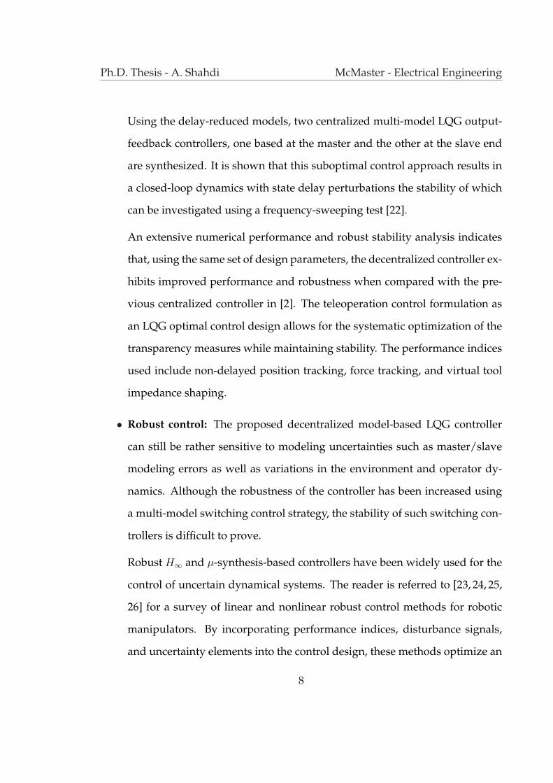
Using the delay-reduced models, two centralized multi-model LQG output-
feedback controllers, one based at the master and the other at the slave end
are synthesized. It is shown that this suboptimal control approach results in
a closed-loop dynamics with state delay perturbations the stability of which
can be investigated using a frequency-sweeping test [22].
An extensive numerical performance and robust stability analysis indicates
that, using the same set of design parameters, the decentralized controller ex-
hibits improved performance and robustness when compared with the pre-
vious centralized controller in [2]. The teleoperation control formulation as
an LQG optimal control design allows for the systematic optimization of the
transparency measures while maintaining stability. The performance indices
used include non-delayed position tracking, force tracking, and virtual tool
impedance shaping.
• Robust control: The proposed decentralized model-based LQG controller
can still be rather sensitive to modeling uncertainties such as master/slave
modeling errors as well as variations in the environment and operator dy-
namics. Although the robustness of the controller has been increased using
a multi-model switching control strategy, the stability of such switching con-
trollers is difficult to prove.
Robust H∞ and µ-synthesis-based controllers have been widely used for the
control of uncertain dynamical systems. The reader is referred to [23, 24, 25,
26] for a survey of linear and nonlinear robust control methods for robotic
manipulators. By incorporating performance indices, disturbance signals,
and uncertainty elements into the control design, these methods optimize an
8

Ph.D. Thesis - A. Shahdi McMaster - Electrical Engineering
`∞ norm of the closed-loop performance of the system while guaranteeing its
stability under a worst-case uncertainty scenario [27, 28]. Robust H∞-based
controllers have been used for delay-free teleoperation [29, 30], as well as
time-delay teleoperation, using a Pade approximation of the delay [31] or
by treating it as a perturbation to the system [32, 33]. Pade approximation is
usually valid at low frequency and can lead to closed-loop instability due to
its inaccuracy, unless very high-order approximations are used. High-order
delay approximations, on the other hand, can cause difficulties in obtaining
a solution to the H∞ control problem. Moreover, the treatment of the de-
lay as a perturbation to system dynamics is unrealistic and can yield overly
conservative control designs specially for larger delays. It is expected that
the inclusion of the time delay information into the design process would
produce far less conservative results.
In this thesis a new mixed adaptive/robust controller is proposed for time-
delay teleoperation. In the first step, local Lyapunov-based adaptive/nonlinear
controllers [34] are used to eliminate the nonlinearities and dynamic uncer-
tainties of the master and slave robots resulting in two linear subsystems with
uncertainty only in the environment and operator dynamics. In the second
step, a robust performance H∞ optimization problem is formulated to en-
hance teleoperation fidelity using transparency-based performance indices
while maintaining stability in the presence of uncertainty in the operator and
environment dynamics. The performance indices include non-delayed po-
sition and force tracking. A robust coordinating controller is synthesized
through recursive solutions to adobe-type problems based on the approach
9
Ph.D. Thesis - A. Shahdi McMaster - Electrical Engineering
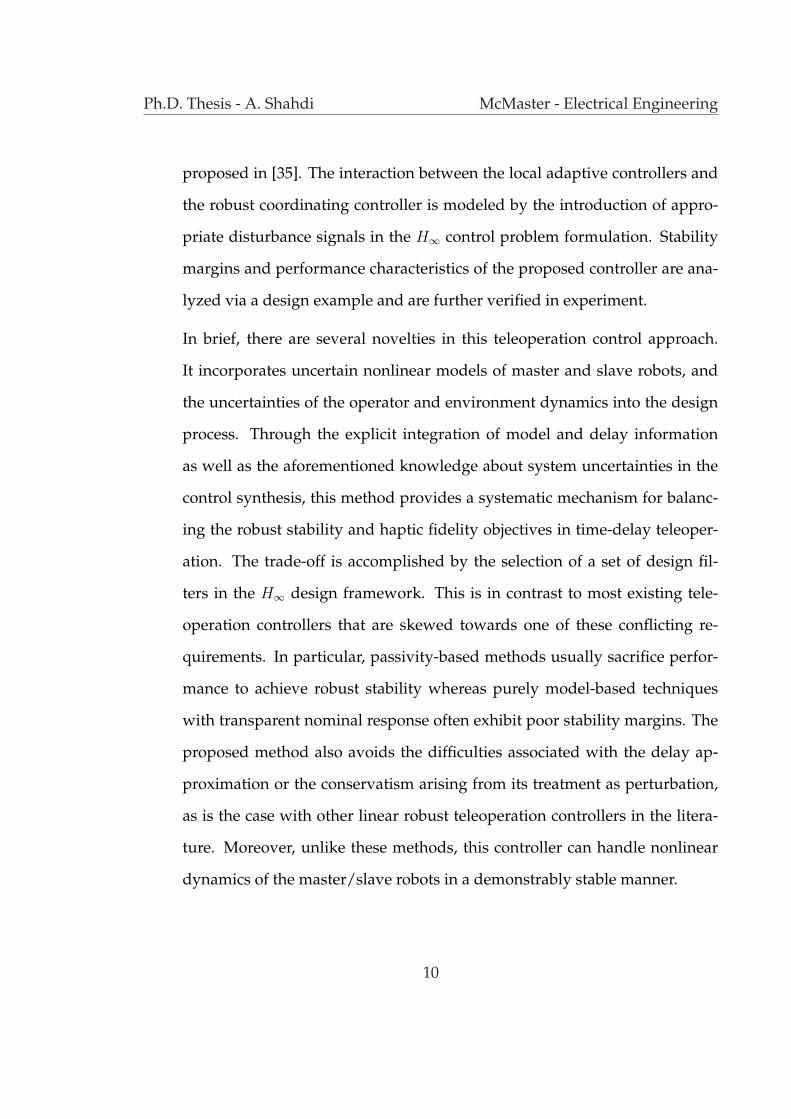
proposed in [35]. The interaction between the local adaptive controllers and
the robust coordinating controller is modeled by the introduction of appro-
priate disturbance signals in the H∞ control problem formulation. Stability
margins and performance characteristics of the proposed controller are ana-
lyzed via a design example and are further verified in experiment.
In brief, there are several novelties in this teleoperation control approach.
It incorporates uncertain nonlinear models of master and slave robots, and
the uncertainties of the operator and environment dynamics into the design
process. Through the explicit integration of model and delay information
as well as the aforementioned knowledge about system uncertainties in the
control synthesis, this method provides a systematic mechanism for balanc-
ing the robust stability and haptic fidelity objectives in time-delay teleoper-
ation. The trade-off is accomplished by the selection of a set of design fil-
ters in the H∞ design framework. This is in contrast to most existing tele-
operation controllers that are skewed towards one of these conflicting re-
quirements. In particular, passivity-based methods usually sacrifice perfor-
mance to achieve robust stability whereas purely model-based techniques
with transparent nominal response often exhibit poor stability margins. The
proposed method also avoids the difficulties associated with the delay ap-
proximation or the conservatism arising from its treatment as perturbation,
as is the case with other linear robust teleoperation controllers in the litera-
ture. Moreover, unlike these methods, this controller can handle nonlinear
dynamics of the master/slave robots in a demonstrably stable manner.
10

Ph.D. Thesis - A. Shahdi McMaster - Electrical Engineering
• Adaptive control: Adaptive controllers can avoid the trade-off between sta-
bility and performance by changing their parameters and/or structure in re-
sponse to variations in system dynamics. The proposed robust controller is
less sensitive to modeling uncertainties compared to our earlier model-based
controllers. Nonetheless, given that a fixed teleoperation controller is used
for the entire range of operation, the transparency may still be sacrificed par-
ticulary if large modeling uncertainty is considered in the design.
To address this problem, in this thesis a new adaptive controller for time-
delay teleoperation is introduced. This approach represents a major step
towards achieving higher transparency while maintaining the stability of a
time-delay bilateral teleoperation system. The proposed method consists of
a model-based predictive control scheme which uses the estimated model of
the system to predict its future states. Using the predicted states, teleopera-
tion coordination is achieved by defining new outputs that are regulated to
zero within an output control framework. A Lyapunov analysis is used to
demonstrate closed-loop stability and to derive the parameters adaptation
law. Another advantage of this controller is its ability to handle known time-
varying latencies in the design procedure.
The proposed method provides a provably stable adaptive predictive con-
troller for teleoperation systems with communication delay. In order to achieve
a high level of transparency, the model and delay information are utilized in
design procedure. The transparency objectives include delay-free position
tracking and tool impedance shaping. The controller also has the ability to
11
Ph.D. Thesis - A. Shahdi McMaster - Electrical Engineering
adapt to uncertainties and changes in user and environment dynamics. Ex-
perimental results demonstrate the effectiveness of the proposed approach
for both constant and time-varying latencies.
It is important to mention that all the proposed controllers are designed in the
continuous-time domain but are implemented in the discrete-time domain. Em-
ploying a fast sampling rate compared to the relatively slower dynamics of the
mechanical system and the desired bandwidth of the tracking objectives ensures
that the discrete-time implementation is a sufficiently accurate approximation of
the original controller.
1.4 Organization of the Thesis
The rest of the thesis is organized as follows. Telerobotic literature has been re-
viewed in Chapter 2. Chapter 3 formulates the nonlinear dynamics of the master
and slave robots. Model-based decentralized control of time-delay teleoperation
systems is presented in Chapter 4. Chapter 5 introduces the robust control archi-
tecture for time-delay teleoperation. The adaptive controller for bilateral teleop-
eration under time delay is presented in Chapter 6. Simulations, robust stability
analysis and experimental results under various scenarios are given for each of
the methods in their corresponding chapters. The thesis is concluded in Chapter 7
where some possible directions for future research are also discussed.
12

Ph.D. Thesis - A. Shahdi McMaster - Electrical Engineering
1.5 Related Publications
1.5.1 Journal Articles
• A. Shahdi and S. Sirouspour, ”Adaptive control for time-delay teleopera-
tion,” To be submitted to IEEE Transactions on Robotics.
• A. Shahdi and S. Sirouspour, ”Model-based decentralized control of time de-
lay teleoperation systems,” The International Journal of Robotics Research, vol.
28, no.3, pp. 376-394, 2009.
• A. Shahdi and S. Sirouspour, ”Adaptive/robust control for time delay tele-
operation,” IEEE Transactions on Robotics, vol. 25, no. 1, pp. 196-205, 2009.
1.5.2 Conference Papers
• A. Shahdi and S. Sirouspour, ”Improved transparency in bilateral teleoper-
ation with variable time delay,” in Proceedings of IEEE/RSJ International Con-
ference on Intelligent Robots and Systems, pp. 4616-4621, St. Louis, Missouri,
2009.
• A. Shahdi and S. Sirouspour, ”Adaptive control of time delay teleoperation
systems,” in Proceedings of Third Joint EuroHaptics Conference and Symposium
on Haptic Interfaces for Virtual Environment and Teleoperator Systems, pp. 308-
313, Salt Lake City, Utah, 2009.
• A. Shahdi and S. Sirouspour, ”Adaptive/robust control for enhanced teleop-
eration under communication time delay,” in Proceedings of IEEE/RSJ Interna-
tional Conference on Intelligent Robots and Systems, pp. 2667-2672, San Diego,
13
Ph.D. Thesis - A. Shahdi McMaster - Electrical Engineering
California, 2007.
• A. Shahdi and S. Sirouspour, ”A multi-model decentralized controller for
teleoperation with time delay,” in Proceedings of IEEE/RSJ International Con-
ference on Intelligent Robots and Systems, pp. 496-501, San Diego, California,
2007.
• P. Setoodeh, S. Sirouspour and A. Shahdi, ”Discrete-time multi-model con-
trol for cooperative teleoperation under time delay,” in Proceedings of IEEE
International Conference on Robotics and Automation, pp. 2921-2926, Orlando,
Florida, 2006.
14
Chapter 2
Literature Review
2.1 Introduction
Teleoperation systems have been subject of extensive research in the past. Var-
ious control methods have been proposed and developed trying to achieve the
two main and often conflicting objectives of teleoperation, i.e. robust stability and
transparency. In a perfectly transparent system the operator feels as he/she is di-
rectly manipulating the task environment.
This chapter presents a survey of the teleoperation control literature under the
following categories: (i) teleoperation control architectures, (ii) control of delay-
free teleoperation systems, (iii) time-delay systems and (iv) time-delay teleopera-
tion control.
15

Ph.D. Thesis - A. Shahdi McMaster - Electrical Engineering
Figure 2.1: A general bilateral teleoperation control architecture.
2.2 Teleoperation Control Architectures
In a bilateral teleoperation system the sensory information, i.e. position/velocity
and/or force signals, are transmitted between the master and slave stations. Fig. 2.1
shows a general teleoperation architecture including all the information exchange
paths.
Teleoperation controllers can be classified with respect to the type of the mea-
surements communicated between the master and the slave sites. In a position-
position architecture, only the position/velocity signals are transmitted over the
communication channel [36]. Other popular architectures are position-force [37,
32], force-force [29], and the four-channel [18,38] controller. In the latter case, both
the position and velocity and the force information are sent between the two sta-
tions as shown in Fig. 2.1. The four-channel teleoperation control can in theory
provide ideal transparency provided that the dynamics of the master and slave
manipulators are known. However, in practice, the variation of these dynamics
can reduce transparency or even cause instability [18, 38, 39]. Another factor that
16
Ph.D. Thesis - A. Shahdi McMaster - Electrical Engineering
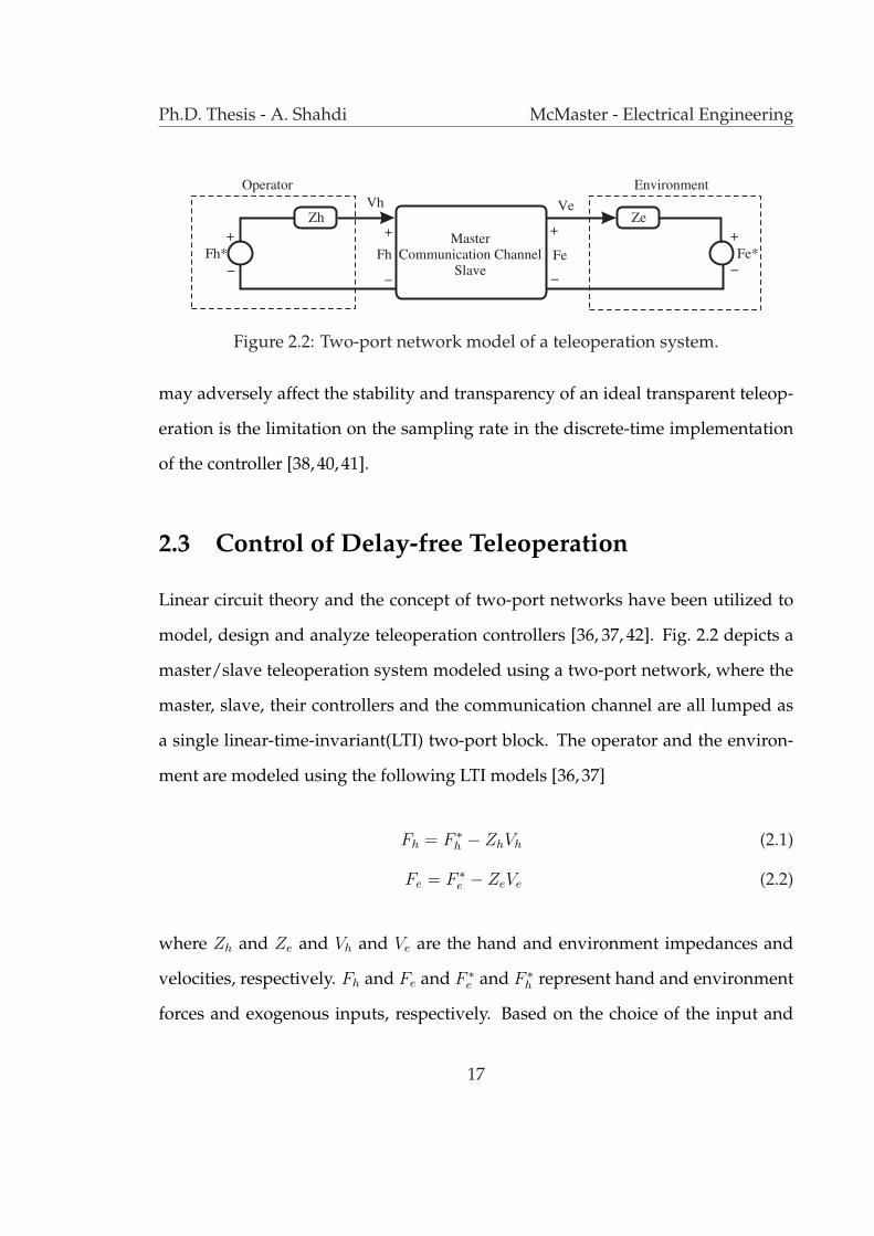
Figure 2.2: Two-port network model of a teleoperation system.
may adversely affect the stability and transparency of an ideal transparent teleop-
eration is the limitation on the sampling rate in the discrete-time implementation
of the controller [38, 40, 41].
2.3 Control of Delay-free Teleoperation
Linear circuit theory and the concept of two-port networks have been utilized to
model, design and analyze teleoperation controllers [36, 37, 42]. Fig. 2.2 depicts a
master/slave teleoperation system modeled using a two-port network, where the
master, slave, their controllers and the communication channel are all lumped as
a single linear-time-invariant(LTI) two-port block. The operator and the environ-
ment are modeled using the following LTI models [36, 37]
Fh = F ∗h − ZhVh (2.1)
Fe = F ∗e − ZeVe (2.2)
where Zh and Ze and Vh and Ve are the hand and environment impedances and
velocities, respectively. Fh and Fe and F ∗e and F ∗
h represent hand and environment
forces and exogenous inputs, respectively. Based on the choice of the input and
17

Ph.D. Thesis - A. Shahdi McMaster - Electrical Engineering
output signals, different network matrices can be defined as [43, 44]
Fh
Fe
=
z11 z12
z21 z22
Vh
−Ve
Impedance Z (2.3)
Vh
−Ve
=
y11 y12
y21 y22
Fh
Fe
Admittance Y (2.4)
Fh
−Ve
=
h11 h12
h21 h22
Vh
Fe
Hybrid H (2.5)
Vh
Fe
=
g11 g12
g21 g22
Fh
−Ve
Inverse Hybrid G. (2.6)
The transparency of a teleoperation system can be formulated using the men-
tioned two-port network representations. In a perfectly transparent system, the
impedance reflected to the operator should be a match to the actual environment
impedance, i.e. [18]
Fh
Vh
∣∣∣∣F ∗e =0
=Fe
Ve
∣∣∣∣F ∗e =0
. (2.7)
In addition, the position/velocity of the master and slave devices should pre-
cisely track each other. Using the hybrid matrix parameters in (2.5) the transmitted
impedance to the operator, Zto, can be expressed as
Zto =h11 + ∆hZe
1 + h22Ze
(2.8)
18
Ph.D. Thesis - A. Shahdi McMaster - Electrical Engineering
where ∆h is defined as
∆h = h11h22 − h12h21 (2.9)
and Ze is the environment impedance. The ideal transparency condition in (2.7)
can be expressed in terms of the hybrid parameters as follows [37, 42]
h11 = h22 = 0
h12 = − h21 = 1. (2.10)
It is worth noticing that a perfect transparent system is marginally absolutely stable
and requires acceleration measurements in its implementation. Hence, to achieve
robust stability, ideal transparency has to be compromised. [18, 42]
The concept of passivity has been utilized to guarantee the stability of teleoper-
ation systems. Consider the two-port network depicted in Fig. 2.2. Such network
is passive if and only if the following condition holds at any time t [45]
∫ t
−∞Fhvh − Feve ≥ −E0 (2.11)
where E0 is the initial energy stored in the network. In other words a passive sys-
tem can only dissipate energy. The system is known to be lossless if the integral
in (2.11) is equal to −E0 as t → ∞. The passivity of the two-port network teleop-
eration in Fig. 2.2 ensures the stability of the system when it is attached to strictly
passive operator and environment dynamics [36, 18]. This is due to the fact that
the connection of passive elements results in a passive system which directly im-
plies its stability provided that F ∗h and F ∗
e inputs are bounded [46]. The passivity
of a two-port network modeled by (2.3) can be formulated in terms of the network
19

Ph.D. Thesis - A. Shahdi McMaster - Electrical Engineering
parameters using Raisbecks’passivity criteria as
Rz11(jω) ≥ 0, (2.12)
Rz22(jω) ≥ 0, (2.13)
4Rz11(jω)Rz22(jω) − (Rz12(jω)+Rz21(jω))2
− (Iz12(jω) − Iz21(jω))2 ≥ 0 (2.14)
for all ω ≥ 0, where R· and I· are equal to the real and imaginary value of
their corresponding arguments.
Passivity condition is however rather conservative. Therefore, other less con-
servative techniques such as structured singular value condition [47] and absolute
stability condition [44] have been utilized to ensure the stability of the system.
Llewellyn’s criteria states that a two-port network modeled by (2.3) is absolutely
stable if and only if [43]
Rz11(jω) ≥ 0, (2.15)
Rz22(jω) ≥ 0, (2.16)
−Rz12(jω)z21(jω)|z12(jω)z21(jω)| + 2Rz11(jω)Rz22(jω)
|z12(jω)z21(jω)| ≥ 1 (2.17)
for all ω ≥ 0, where | · | represents the absolute value operator.
Researchers have used the two-port network model for teleoperation control
design. Hannaford [37] proposed a bilateral impedance control architecture using
a hybrid two-port model. Hashtrudi-zaad and Salcudean [42] gave a comprehen-
sive review of the teleoperation controllers utilizing two-port network models. In
20
Ph.D. Thesis - A. Shahdi McMaster - Electrical Engineering
this article, the extension of the controller design from two-channel impedance
controller to four-channel bilateral teleoperators with either impedance or admit-
tance models is investigated. Also, the set of control parameters that provide the
system with ideal transparency are calculated for each type of teleoperation. The
surveyed control methods so far often sacrifice either the transparency or the sta-
bility of teleoperation in favor of the other. To facilitate a systematic approach to
balance these conflicting teleoperation objectives, more sophisticated control ar-
chitectures have been utilized in the literature.
2.3.1 Robust Controllers
Linear controllers based on the H∞ and µ-synthesis theories have been developed
for the control of robotic manipulators to achieve robust stability and enhanced
performance in the presence of uncertainties in the system dynamics. The reader
is referred to [26] for a survey of linear and nonlinear robust control methods for
robotic manipulators. By incorporating performance indices, disturbance signals,
and uncertainty elements into the control design, these methods optimize an `∞
norm of the closed-loop performance of the system while guaranteeing its stability
under a worst-case uncertainty scenario [25, 24, 48, 49, 50].
In the context of teleoperation, these robust controller design methods have
been utilized to achieve robust stability and transparency [32, 47, 31, 30]. Col-
gate [47] introduced an impedance shaping control technique for teleoperation
systems. A general condition for the robustness of a bilateral teleoperator is cal-
culated using the structured singular value(µ). Kazerooni et. al. [29] proposed a
control method based on H∞-optimal control for force-force teleoperation systems.
21
Ph.D. Thesis - A. Shahdi McMaster - Electrical Engineering
In [31], a general H∞ framework has been proposed for four-channel bilateral tele-
operation control. Hu et. al. [51] formulated the controller design as a multiple
objective optimization problem and incorporated robust stability into the design
of the controller. Recently, Sirouspour [52] proposed a robust controller for multi-
master/multi-slave cooperative teleoperation based on µ-synthesis.
Passivity based methods have been developed for the control of teleoperation
systems in order to ensure robust stability in the presence of a wide range of un-
certainties. Ryu et al. [53] have proposed an energy-based method for stable tele-
operation using the time-domain passivity control under no communication delay.
Based on the concept of passive decomposition, the authors in [54] proposed a non-
linear controller that can provide useful task-specific dynamics for inertia scaling,
motion guidance, and obstacle avoidance.
These robust control approaches can often lead to conservative controllers es-
pecially when the uncertainty range in the dynamics parameters are large which is
usually the case in teleoperation systems. This is due to the fixed structure and/or
parameters of the controller. Passivity-based control designs also often tend to sac-
rifice transparency objectives in favor of robust stability. This is due to the fact that
these controllers have to maintain system’s stability for all passive environment
and arm dynamics.
2.3.2 Adaptive Controllers
Variable controller parameters and/or structure help adaptive controllers avoid
the trade-off between system’s performance and stability. Kress and Jansen [55]
have introduced a tuning technique for a telerobotic arm controller which can
22
Ph.D. Thesis - A. Shahdi McMaster - Electrical Engineering
automatically determine the set of optimal controller gains for a simple PD con-
troller by utilizing an intelligent search technique. Hashtrudi-zaad and Salcud-
ean [56] have proposed a class of indirect adaptive bilateral control schemes. Their
method uses measurements of master and slave position, velocity and accelera-
tion to estimate the environment impedance. Shi et al. [57] have introduced new
transparency concepts suitable for adaptive control of teleoperation systems with
time varying parameters. In [34], local master/slave adaptive nonlinear posi-
tion/force controllers have been combined with teleoperation coordinating con-
trollers to guarantee stable teleoperation in the presence of dynamic uncertainty.
The proposed method is applicable to both unilateral and bilateral teleoperation
systems and in both position and rate control modes. The uncertainties in hand
and environment dynamics are taken care of by adding these dynamics to the mas-
ter and slave dynamics and applying the local adaptive controllers. Some other
adaptive teleoperation control schemes can be found in [58, 59].
In the decentralized control method proposed in this thesis, a multiple-model
adaptive controller is used for teleoperation in unknown environments. Multiple-
model controllers assume that system dynamics obey a model from a given finite
set of models, with known or unknown parameters. These methods have previ-
ously been used for the control of robot manipulators. Ciliz and Narendra [60]
utilized multiple models of a manipulator for identifying its unknown inertial pa-
rameters as well as the parameters of its load. Leaby and Sablan [61] augmented a
mode-based controller with multiple-model adaptive estimation to minimize posi-
tion trajectory tracking errors. Narendra and Balakrishnan [62] presented a general
methodology for adaptive control using multiple models, switching and tuning.
23
Ph.D. Thesis - A. Shahdi McMaster - Electrical Engineering
They proposed specific performance indices in terms of model outputs and how
to choose the best model using these indices. Zhang and Jiang [63] adopted inter-
acting multiple model (IMM) filters to develop an active fault tolerant controller.
In the proposed decentralized method, the change in the slave/environment
dynamics due to rigid contact, and parameter variations due to flexible contact,
is handled with a multi-model control approach, in which mode-based controllers
are designed for different phases of the operation. Switching between these mode-
based control laws occurs according to the identified contact mode.
2.4 Time-delay Teleoperation Control
In applications in which the master and slave sites are at a distance from each other,
communication time delay can severely degrade the transparency and stability of
conventional teleoperation methods [18,64,8]. This latency imposes a trade-off be-
tween the conflicting requirements of stability and performance with the potential
for instability increasing by the level of the performance [18, 64]. A well-balanced
trade-off between robust stability and performance can only be achieved by care-
fully incorporating knowledge about system model, time delay and modeling un-
certainty in the control design process.
The trade-off between the stability and the transparency of time-delay teleop-
eration systems can be clearly noticed in the comparison of unilateral and bilateral
controllers. Using high bandwidth position/veolcity and/or force feedback loops,
bilateral teleoperators can provide kinesthetic coupling and a more faithful ren-
dering of the environment to the operator. However, this makes them far more
susceptible to instability issues caused by the delay in communication channel.
24

Ph.D. Thesis - A. Shahdi McMaster - Electrical Engineering
On the other hand, unilateral teleoperators in which the operator merely receives
visual feedback from the task environment are more robust with respect to the time
delay [8].
In [64], the robust stability of a number of bilateral teleoperation architectures
with respect to time delay is analyzed. Arcara and Melchiorri [65] have compared
some existing teleoperation control schemes that address the issue of time delay
from stability and performance perspectives. Imaida et. al. [66] have shown that,
by providing sufficient damping at the master and slave ends, a delayed bilateral
position-position teleoperation system can be stabilized, though at the expense
of a sluggish response. In [67] a quantitative evaluation of operability has been
investigated that depends on the communication time delay.
Lee and Lee [68] have proposed the concept of telemonitoring force feedback
as a form of kinesthetic coupling for teleoperation under delays of up to a few sec-
onds. The performance of the teleoperation system is optimized assuming delays
of up to a known maximum value. In [69], state convergence has been used for
time-delay teleoperation control design. In this method, master and slave manip-
ulators are represented in linear state-space form and the delay is approximated
using a first-order Taylor’s expansion. Mirfakhrai and Payandeh [70] have devel-
oped a stochastic model for time delay over the Internet, which is becoming more
popular as a communication medium.
2.4.1 Passivity-based Controllers
A large number of existing time-delay teleoperation controllers employ the scatter-
ing theory and the concept of passivity to attain guaranteed stability, e.g. see [71,
25

Ph.D. Thesis - A. Shahdi McMaster - Electrical Engineering
72, 73, 74, 75, 76] among other references. A survey on passivity based controllers
for time-delay teleoperation can be found in [77].
The introduction of wave variables enabled researchers to analyze and design
stable force-reflecting teleoperation controllers. Based on the concepts of power
and energy, wave variable transformation can handle large uncertainties and un-
known models. A pair of wave variables, (u,w), can be defined based on a pair of
velocity and force signals, (v, f), and using the following equations
u =bv + f√
2b, (2.18)
w =bv − f√
2b(2.19)
where b is positive scalar and can be used as a tuning parameter. Assuming the
following power flow for a pair of velocity and force signals
P = vT f (2.20)
and using the definitions in (2.18) and (2.19), the power flow can be written as a
function of the wave variables as
P =1
2uT u− 1
2wT w. (2.21)
It is worth mentioning that the contribution of the signal u is always positive and
the contribution of the signal w is always negative.
The wave variable transformation and the concept of passivity have enabled
researchers to develop stable controllers for time-delay teleoperation in presence
26

Ph.D. Thesis - A. Shahdi McMaster - Electrical Engineering
of uncertainties. In [71], it has been shown that for a time-delay teleoperation sys-
tem, the master/slave control laws can be chosen such that the two-port model of
the system is rendered passive. This ensures the stability of the system in contact
with all passive arm and environment dynamics and irrespective of the amount of
time delay. Niemeyer and Slotine [73] used the idea of passivity to provide energy
conservation and to guarantee system’s stability in the presence of an unknown
time-delay. In [78], the authors have introduced an energy balance monitoring
method to limit the generated energy by the system and achieve passivity in pres-
ence of time-varying communication delay.
Yokokohji et. al. [79] proposed a control scheme based on wave variables which
minimizes the performance degradation in spite of time delay fluctuations. Benedetti
et al. [80] introduced a force-feedback teleoperation controller based on wave-
variables for variable time delays. In [81] a passivity-based controller was de-
veloped which can match the system parameters with changes in the delay by
predicting the future values of delay. Ueda and Yoshikawa [76] presented a force-
reflecting teleoperation controller with time delay using wave transmission meth-
ods. Conditions of stability for the proposed controller were also derived.
In passivity-based methods, enhanced robust stability is often gained at the ex-
pense of a highly reduced transparency. Consequently, several variations of the
wave transformation-based control approach have been developed to improve its
transparency. In [82], an adaptation of line terminating impedance functions was
proposed to remedy the loss of transparency in bilateral teleoperation based on
the scattering theory. In [83], a wave-based teleoperation controller has been com-
bined with a Smith Predictor, a Kalman filter, and an energy regulator to improve
27
Ph.D. Thesis - A. Shahdi McMaster - Electrical Engineering
its transparency. The passivity has been used to enhance the performance of a
proportional-derivative type time-delay teleoperation controller in [84].
In [85], new passive outputs were defined for master and slave robots which
include position and velocity information. These outputs were then utilized to
couple the master and slave devices and to enhance the teleoperation transparency.
In [86], wave filtering and shaping have been employed to reduce the damping
resulted from impedance matching. Furthermore, a high frequency force feedback
at the slave side was used to increase the fidelity of teleoperation. Finally in [87],
the authors have combined wave variables and a model-based slave predictor to
achieve stability and reduce undesirable effects of the wave variable approach on
the performance. A direct drift control scheme was also used to minimize the drift
caused by the errors in the slave model.
2.4.2 Robust Controllers
Robust controllers have been utilized in the literature to control teleoperation sys-
tems in presence of time delay. In [31], a controller design based on the H∞ theory
has been presented. In this paper, a Pade approximation of the delay is employed.
Pade approximation is usually valid at low frequency and can lead to closed-loop
instability due to its inaccuracy, unless high-order approximations are used. High-
order delay approximations, on the other hand, can lead to difficulties in obtain-
ing a solution to the H∞ control problem. In [32], H∞ and µ-synthesis methods
have been used to design a stable teleoperation controller for a predefined delay
maximum. Sename and Fattouh [33] have proposed a controller that stabilizes the
teleoperation system in presence of environment uncertainties and independent of
28

Ph.D. Thesis - A. Shahdi McMaster - Electrical Engineering
the amount of time delay. In both [32, 33] the delay in teleoperation is treated as
a perturbation to the system. The treatment of the delay as a perturbation to dy-
namics is unrealistic and can yield overly conservative control designs. This is due
to the fact that the model of the system and delay are not being effectively used in
the controller design.
2.4.3 Predictive Controllers
Heuristic techniques such as predictive displays and virtual environments rely on
accurate models of the task environment to provide the operator with a realis-
tic delay-free simulated response of the remote manipulator and environment for
teleoperation under time delays up to several seconds [8, 88, 89, 90]. In [91], lo-
cal models of the environment have been utilized to deliver predictive displays as
well as delay-free simulated force-feedback to the operator. The local models uti-
lized in the mentioned predictive display controllers can interact with the actual
environment using the measurements received from the slave site through intro-
ducing the concept of time clutches [92,93,94]. The complexity of building accurate
local models for unstructured environments and stability issues pertaining to real-
time model identification and update limit the utility of such approaches in many
applications.
Predictive control methods such as the Smith Predictor have also been devel-
oped for teleoperation [65, 83]. Ganjefar et al. [95] have discussed the behavior
of Smith Predictor in teleoperation systems with respect to modelling and time
delay errors. In [96] a predictive model-based controller has been proposed for
29

Ph.D. Thesis - A. Shahdi McMaster - Electrical Engineering
teleoperation with time-delay using state prediction. Different predictive force-
feedback methods are also presented. References [97] and [98] have proposed pre-
dictive controller techniques for teleoperation with unbounded delays. Prekopiou
et. al. [99] have developed a predictive controller for teleoperators based on a pre-
diction of the user position and force. Polynomial or spline predictor have been
used to predict the master’s state. The method has shown a good performance in
simulations, for short time delays and smooth hand movements. Nevertheless, ex-
cluding the arm dynamics in the control design can result in reduced transparency
or even cause instability. Also, the stability of such predictive controller is not
guaranteed.
Model-based predictive controllers have been successfully utilized in [1] and [2]
to reduce the time-delay teleoperation system to a delay-free system in discrete
and continuous-time, respectively. Linear Quadratic Gaussian controllers are then
applied to the delay-free systems to achieve tracking objectives. Although multi-
model switching strategies are used to increase the robustness of these controllers,
they are still sensitive to modeling uncertainties, e.g. modeling errors in mas-
ter/slave as well as operator arm and environment dynamics. Also, an additional
time delay is introduced in the control loop due to the centralized structure of these
controllers. The additional delay can potentially increase the controllers sensitivity
to modeling uncertainties.
2.5 Time-delay Systems
There has been considerable effort in stability analysis and control synthesis for
time-delay systems. This section is not a comprehensive review of the literature
30

Ph.D. Thesis - A. Shahdi McMaster - Electrical Engineering
on time-delay systems and focuses only on the approaches related to the methods
proposed in this thesis. Interested reader is referred to the following survey papers
on this topic [100, 101, 102]. Also, methods for robust stability analysis of systems
with time delay can be found in the survey papers [103, 104].
Kwon et al. [105] and later Artstein [106] introduced a transformation to reduce
an infinite-dimensional continuous-time linear control system with delayed con-
trol actions to an equivalent control system without delay. Consider a multi-input
linear delay system with the following state-space dynamics
X(t) = AX(t) +
nI∑j=1
Bjuj(t− djI) (2.22)
where X(t) is the vector of states, uj(t) is the j’th input vector, nI is the number of
inputs and djI is the delay in the j’th input channel. By taking the derivative of a
new state Z(t) defined below
Z(t) = X(t) +
nI∑j=1
∫ t
t−djI
eA(t−s−djI)Bjuj(s)ds (2.23)
and substituting X(t) from (4.45), one may write
Z(t) = AZ(t) +
nI∑j=1
e−AdjIBjuj(t). (2.24)
The new system in (2.24) has no delay in its control signals and therefore, standard
control methods such as state-feedback can be implemented for its stabilization.
Systems with delays in both input and output channels can simply be converted
31

Ph.D. Thesis - A. Shahdi McMaster - Electrical Engineering
to an equivalent system with delays in inputs, if the delays in all output or all in-
put ports are equal. However, teleoperation control systems involve non-identical
delays in their input and output channels and this transformation in its original
form is not suitable for such systems. A modified version of the transformation
is introduced in this thesis and is utilized in the decentralized model-predictive
teleoperation controller in Chapter 4.
An increased interest in the robust H∞ control of time-delay systems since
late 1990s has yielded several new results in this area, i.e. see [107, 108]. Most
researchers have approached the problem as designing controllers for infinite-
dimensional systems resulting in rather abstract and complex solutions unsuitable
for the use in practical applications. In contrast in the work of [109] and [35],
the treatment of the delay as a constraint on the controller has produced elegant
tractable solutions to the H∞ control of multi-input/multi-output (MIMO) systems
with input/output (I/O) delays. In this method, a robust controller is synthesized
through recursive solutions to adobe-type problems. Through explicit integration
of model and delay information as well as the knowledge about system uncer-
tainties in the control synthesis, this method provides a systematic mechanism for
balancing the robust stability and performance objectives in time-delay systems.
Several schemes for adaptive control of time-delay systems have been proposed
in the literature. Interested reader is refereed to [110, 111] for a survey of such
controllers. In [112], an adaptive controller for a class of input-delayed system
has been presented. This control architecture depended on the relative degree of
the plant transfer function. The stability of the closed-loop system is investigated
through a Lyapunov-Krasovskii analysis. In [113] a modified reduction method
32
Ph.D. Thesis - A. Shahdi McMaster - Electrical Engineering
has been introduced which uses estimates of system parameters. These parame-
ter estimates are updated by utilizing the measurements. However, this method
is only applicable to single-input/single-output first-order systems and was never
extended to more general forms of dynamics. In this thesis, we propose a new de-
lay reduction technique which can be applied to an uncertain multi-input/multi-
output system such as that in time-delay teleoperation.
33
Chapter 3
Teleoperation Dynamics and
Performance Objectives
3.1 Introduction
This chapter studies the dynamics of the teleoperation system components, i.e. the
master and slave robots as well as the operator’s arm and the environment. In
addition, the performance objectives in teleoperation control are discussed.
The chapter is organized as follows. In Section 3.1, the equations of motion
of teleoperation subsystems are derived. Several properties of these dynamics are
shown and at the end the combined nonlinear dynamics of the master/hand and
slave/environment are presented. In Section 3.2, the performance objectives of
teleoperation control are illustrated in the form of ideal transparency and its alter-
native, virtual tool impedance shaping.
34
Ph.D. Thesis - A. Shahdi McMaster - Electrical Engineering
3.2 Robot Dynamics
The master and slave robots in teleoperation are generally rigid multi-body me-
chanical manipulators. The dynamics of such manipulators can be expressed ei-
ther in the joint-space or the work-space coordinates. Two different methods can be
utilized to obtain the manipulator dynamics in the joint-space, i.e. the Newton-
Euler recursive method and Lagrange formulation [114]. The Newton-Euler formu-
lation is a numerical method and leads to a recursive type of solution for manipu-
lator dynamics. It incorporates a forward recursion for propagating link velocities
and accelerations and a backward recursion for propagating forces. On the other
hand in the Lagrange method, the equations of motion are derived in a systematic
way and independent of the reference coordinate frame and gives a closed-form
solution for the dynamics. This method provides valuable insight about the nature
of the system dynamics and is utilized in this thesis to obtain the dynamics of the
teleoperation system.
For an n-degree-of-mobility robot, the generalized coordinates are defined as a set
of variables λi, i = 1, . . . , n, which describe the link positions of the manipulator.
Joint variables are the natural choice for the generalized coordinated for an open-
chain mechanical manipulator
q =
λ1
...
λn
. (3.1)
To derive the equations of motion of the mechanical system using the Lagrange
35

Ph.D. Thesis - A. Shahdi McMaster - Electrical Engineering
method, first the Lagrangian of the system is defined as a function of the general-
ized coordinates [114]
L(q, q) = T (q, q)− U(q) (3.2)
where T and U are the kinetic and potential energy of the system, respectively. The
total kinetic energy of the n-link manipulator can be calculated using the following
sum
T (q, q) =n∑
i=1
(Tli + Tmi) (3.3)
where Tli and Tmi are the kinetic energies of the link i and the link i actuator, and
are functions of the joint positions and velocities, i.e. q and q. The total potential
energy stored in the manipulator is a function of joint positions and is obtained
using the following sum
U(q) =n∑
i=1
(Uli + Umi) (3.4)
where Uli and Umi are the contributions of the link i and its actuator to the potential
energy. See [114] for the actual forms of the kinetic and potential energies in (3.3)
and (3.4).
Using 3.2, the Lagrange’s dynamics equations are formulated by the following
equation setd
dt
∂L∂λi
− ∂L∂λi
= ξi , i = 1, . . . , n (3.5)
where ξi is the generalized force associated with the generalized coordinate λi. The
generalized forces include the joint actuator torques, the joint friction torques, and
36

Ph.D. Thesis - A. Shahdi McMaster - Electrical Engineering
the torques induced by the forces at the end-effector in contact with the environ-
ment. It can be shown that using (3.2) and (3.5), the dynamics of an n-link manip-
ulator in the joint-space can be written in the following compact matrix form
D(q)q + C(q, q)q + G(q) = τ − JT (q)h (3.6)
where D(q) is the inertia matrix, C(q, q) matrix represents velocity dependent ele-
ments such as Coriolis and centrifugal effects, G(q) corresponds to position-dependent
forces such as the gravity, τ is the vector of the joint actuator torques, J is the ge-
ometric Jacobian of the manipulator and h represents generalized external forces
acting at the end-effector. The dynamics equations presented in (3.6) have the fol-
lowing properties [114, 115, 45].
Property 1. The inertia matrix, D(q), is symmetric and uniformly positive-definite
for ∀q ∈ Rn. It also satisfies the following inequality
m1||α||2 ≤ αT D(q)α ≤ m2||α||2 ∀α ∈ Rn (3.7)
where || · || is standard euclidean norm, and m1 and m2 are known positive con-
stants.
Property 2. For a particular choice of C(q, q) based on the Christoffel symbols, the
following skew-symmetry property holds
αT
(1
2D(q)− C(q, q)
)α = 0 , ∀α ∈ Rn. (3.8)
For α equal to q, the property in (3.8) holds for all choices of the matrix C(q, q).
37

Ph.D. Thesis - A. Shahdi McMaster - Electrical Engineering
Property 3. The dynamics in (3.6) can be expressed in the linear-in-parameter form
as follows
D(q)q + C(q, q)q + G(q) = Y (q, q, q)θ (3.9)
where Y (.) is a regressor matrix and is a function of joint positions, velocities and
accelerations and θ is a vector of unknown parameters.
Property 4. The norm of C(q, q) is bounded as
||C(q, q)|| ≤ β||q|| (3.10)
where β is a positive constant.
In the work-space coordinates, the manipulator dynamics can be expressed in
the following form [114]
DA(X)X + CA(X, X)X + GA(X) = ϑA − h (3.11)
where X ∈ R6 is the generalized workspace position vector, h is defined in (3.6)
and ϑA is the contribution of the end-effector forces due to joint actuation, τ . ϑA
and τ are related by the geometric jacobian, J(q), through the following equation
τ = JT (q)ϑA. (3.12)
Matrices DA, CA and GA in the work-space dynamics in (3.11) can be calculated
38
Ph.D. Thesis - A. Shahdi McMaster - Electrical Engineering
based on the matrices D, C and G in the joint-space dynamics (3.6) as follows
DA = J−T DJ−1
CAx = J−T Cq −DAJ q
GA = J−T G. (3.13)
It can be shown that the work-space dynamics in (3.11) inherits all the properties
of the joint-space dynamics in (3.7)-(3.10).
3.3 Teleoperation System Dynamics
The dynamics of the master (γ = m) and slave (γ = s) robots can be written in the
form of (3.11) as
Dγ(Xγ)Xγ + Cγ(Xγ, Xγ)Xγ + Gγ(Xγ) = F ncγ − Fext,γ (3.14)
where F ncγ ∈ R6 is the robots control force. The external end-effector forces on the
master and slave robots correspond to Fh and Fe which are the hand and environ-
ment forces, respectively.
In general, the dynamics of the hand can be nonlinear, time-dependent, posture-
dependent and subject-dependent [116,117,34]. Linear-time-invariant models have
been employed by previous researchers in their work to approximate these dynam-
ics. Such models have been effective in modeling and control of the manipulators
while operated by the human arm [117, 34]. Based on these results, the following
second-order decoupled linear-time-invariant (LTI) dynamics are considered for
39
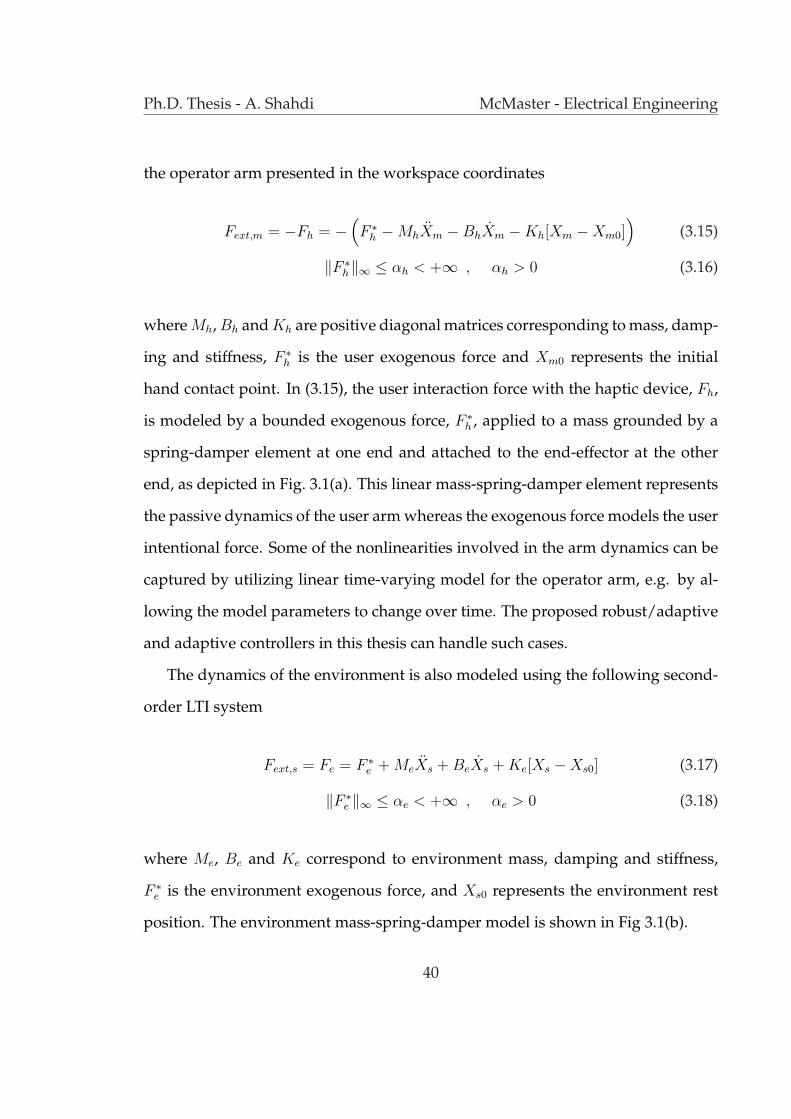
Ph.D. Thesis - A. Shahdi McMaster - Electrical Engineering
the operator arm presented in the workspace coordinates
Fext,m = −Fh = −(F ∗
h −MhXm −BhXm −Kh[Xm −Xm0])
(3.15)
‖F ∗h‖∞ ≤ αh < +∞ , αh > 0 (3.16)
where Mh, Bh and Kh are positive diagonal matrices corresponding to mass, damp-
ing and stiffness, F ∗h is the user exogenous force and Xm0 represents the initial
hand contact point. In (3.15), the user interaction force with the haptic device, Fh,
is modeled by a bounded exogenous force, F ∗h , applied to a mass grounded by a
spring-damper element at one end and attached to the end-effector at the other
end, as depicted in Fig. 3.1(a). This linear mass-spring-damper element represents
the passive dynamics of the user arm whereas the exogenous force models the user
intentional force. Some of the nonlinearities involved in the arm dynamics can be
captured by utilizing linear time-varying model for the operator arm, e.g. by al-
lowing the model parameters to change over time. The proposed robust/adaptive
and adaptive controllers in this thesis can handle such cases.
The dynamics of the environment is also modeled using the following second-
order LTI system
Fext,s = Fe = F ∗e + MeXs + BeXs + Ke[Xs −Xs0] (3.17)
‖F ∗e ‖∞ ≤ αe < +∞ , αe > 0 (3.18)
where Me, Be and Ke correspond to environment mass, damping and stiffness,
F ∗e is the environment exogenous force, and Xs0 represents the environment rest
position. The environment mass-spring-damper model is shown in Fig 3.1(b).
40

Ph.D. Thesis - A. Shahdi McMaster - Electrical Engineering
Figure 3.1: Linear mass-spring-damper models of (a) the operator’s arm and (b)the environment.
Using (3.14), (3.15) and (3.17), the dynamics of the master robot incorporating
the human operator and the dynamics of the slave robot incorporating the envi-
ronment can be represented by
MmXm + CmXm + Gm = F ncm + F ∗
h (3.19)
Mm = Dm(Xm) + Mh , Cm = Cm(Xm, Xm) + Bh
Gm = Gm(Xm) + Kh[Xm −Xm0]
and
MsXs + CsXs + Gs = F ncs + F ∗
e (3.20)
Ms = Ds(Xs) + Me, Cs = Cs(Xs, Xs) + Be
Gs = Gs(Xs) + Ke[Xs −Xs0].
It can be shown that the master/hand and slave/environment dynamics in (3.19)
and (3.20) hold the properties in (3.7)-(3.10).
41

Ph.D. Thesis - A. Shahdi McMaster - Electrical Engineering
3.4 Performance of Master/Slave Teleoperation Systems
The performance of a bilateral teleoperation system is often measured by how well
it is able to convey to the operator the perception of direct interaction with the ac-
tual or scaled task environment. Ideal transparency, also known as ideal kinesthetic
coupling [38], can be described in terms of scaled position and force tracking be-
tween the master and slave robots [38, 7], i.e.
fh(t) = αffe(t) (3.21)
xm(t) = αpxs(t) (3.22)
where αf and αp denote the force and position scaling factors, respectively. Fig. 3.2(a)
shows the interaction of the operator and the environment through an ideally
transparent teleoperation system with unity position and force scaling factors. In
this case there is a rigid dynamic-less connection between the operator arm and
the environment. Acceleration measurement or equivalently force measurement,
and an exact knowledge of the master and slave dynamics are required for achiev-
ing ideal transparency [38]. In practice, however, modeling and sensing errors,
computation and control delays, and sampling rate limitations in a discrete-time
implementation of the control can easily cause instability in an ideally transparent
teleoperation system [38, 41].
To alleviate these robustness issues with the ideal transparency, a virtual in-
tervening tool can be introduced between the operator and the environment as
42
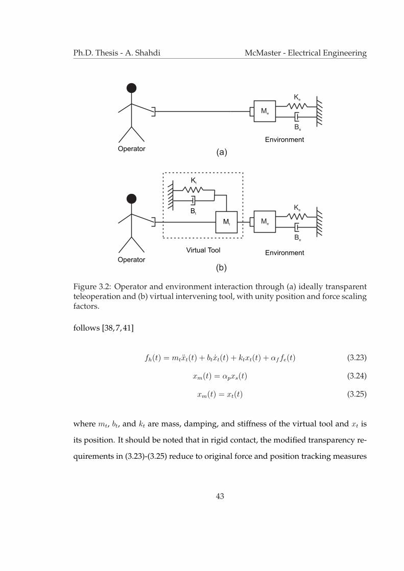
Ph.D. Thesis - A. Shahdi McMaster - Electrical Engineering
Figure 3.2: Operator and environment interaction through (a) ideally transparentteleoperation and (b) virtual intervening tool, with unity position and force scalingfactors.
follows [38, 7, 41]
fh(t) = mtxt(t) + btxt(t) + ktxt(t) + αffe(t) (3.23)
xm(t) = αpxs(t) (3.24)
xm(t) = xt(t) (3.25)
where mt, bt, and kt are mass, damping, and stiffness of the virtual tool and xt is
its position. It should be noted that in rigid contact, the modified transparency re-
quirements in (3.23)-(3.25) reduce to original force and position tracking measures
43
Ph.D. Thesis - A. Shahdi McMaster - Electrical Engineering
in (3.21)-(3.22), if kt = 0. The virtual tool between the operator and the environ-
ment is depicted in Fig. 3.2(b).
As (3.23) and Fig. 3.2(b) suggest, in free motion the operator perceives the
tool dynamics as he/she moves the master device. Also, in contact with the en-
vironment, the interaction between the operator and the environment feels like
manipulating the environment through the virtual tool. Employing a tool with a
high impedance would hinder the operator movements in free motion and inter-
fere with the operator’s perception of the environment in contact. Therefore, it
is desired to keep the tool impedance as low as possible to achieve a more trans-
parent response. However, as shown in [41], computation delays and sampling
rate limitations in a discrete-time implementation limit the lowest achievable tool
impedance.
It is worth noticing that the ideal transparency objectives introduced in this
chapter are based on delay-free tracking measures. Alternatively, the desired per-
formance objectives can be revised to include delayed force and position tracking.
However, in this case the operator would perceive a distorted form of the envi-
ronment impedance since the reflected force would be subject to a round-trip de-
lay with respect to the position of the operator arm. Delay-free teleoperation, if
achievable, would present the operator with the actual impedance of the remote
environment. If needed, the visual display can also include a predictive element
to avoid any discrepancy between visual and haptic feedback. The proposed con-
trollers in this thesis will utilize model-based prediction mechanisms in attempt to
approach such delay-free tracking goals by using any available model and sensor
information. Achieving perfect prediction, however, requires an exact knowledge
44

Ph.D. Thesis - A. Shahdi McMaster - Electrical Engineering
of the system dynamics and more importantly the future of the hand and environ-
ment exogenous inputs to the system and is not possible in practice.
45

Chapter 4
Model-based Decentralized Control
of Time-delay Teleoperation Systems
4.1 Introduction
In a centralized architecture the teleoperation controller resides either at the master
or the slave side. Fig. 4.1 shows a general centralized teleoperation control with
the controller at the master side. In our earlier contributions [1, 2], model-based
centralized controllers were proposed to enhance the performance of teleoperation
by incorporating model and delay information in controller design. One drawback
of such control schemes is the extra delay introduced either in the master or the
slave control path. In Fig. 4.1, this extra delay can be clearly noticed between the
slave measurement and control. By removing this delay through the use of two
local controllers at each station, a decentralized control scheme can potentially lead
to a system with higher stability margins and a better performance. Built on the
earlier results in [2], in this chapter a model-based decentralized control scheme
46

Ph.D. Thesis - A. Shahdi McMaster - Electrical Engineering
Figure 4.1: A centralized teleoperation architecture with controller at the mastersite.
for time-delay bilateral teleoperation is proposed to improve its robust stability
while maintaining a high level of transparency. This is achieved through the use
of delay-free local and delayed remote measurements by the two local controllers
at the master and slave stations. Using the similar approach as in [2], a model-
based delay reduction technique is utilized to obtain two centralized LQG output-
feedback controllers. The stability margins of such control scheme is investigated
using a frequency-sweeping test [22].
The chapter is organized as follows. An adaptive Lyapunov based lineariza-
tion of the master and slave nonlinear dynamics is introduced in Section 4.2. The
integration of the teleoperation dynamics and transparency objectives into a two-
station decentralized control system is presented in Section 4.3. The proposed
state/observation transformations for delay reduction and the two-station decen-
tralized control of the resulting system are discussed in Section 4.4. The results of
numerical performance and robust stability analysis are presented in Section 4.5.
Experimental results are discussed in Section 4.6. The chapter is concluded in Sec-
tion 4.7.
47

Ph.D. Thesis - A. Shahdi McMaster - Electrical Engineering
4.2 Linearization of Master/Slave Teleoperation Sys-
tems Dynamics
As demonstrated in (3.9) and to facilitate the development of adaptive Lyapunov-
based linearization, the master device dynamics in (3.14) are rewritten in an equiv-
alent linear-in-parameter format as follows [114]
D(Xm)Xm + C(Xm, Xm1)Xm2 + G(Xm) = Y (Xm, Xm1, Xm2, Xm)θ (4.1)
where Y (.) is a regressor matrix function of motion variables and known constants,
and θ is a vector of unknown parameters. The following theorem is concerned with
adaptive dynamic linearization of the nonlinear robot dynamics.
Theorem 4.1: Consider the robot dynamics in (3.14) and the following control law
F ncm = −Fh + Y (Xmr, Xm, Xmr, Xm)θ −Kdρm (4.2)
with
Xmr = Xmd − ΛXm, Xm = Xm −Xmd, ρm = ˙Xm + ΛXm
Xmd = L−1 (s2Mm + sBm + Km)−1 (Fh + Fcm) (4.3)
where Mm, Bm, Km > 0 are diagonal matrices, L−1. is the inverse Laplace trans-
form, s is the Laplace variable, and Kd > 0. Also θ is a parameter estimate vector
48
Ph.D. Thesis - A. Shahdi McMaster - Electrical Engineering
with the adaption law
˙θi =
0 if −[ΓY T ρm]i > 0, θi > θmaxi
0 if −[ΓY T ρm]i < 0, θi < θmini
−[ΓY T ρm]i otherwise
(4.4)
where Γ = ΓT > 0, [.]i denotes the i’th element of the argument vector, and θmini and
θmaxi are a priori known lower and upper bounds on the corresponding unknown
parameter. Then the closed-loop dynamics are governed by
Mm¨Xm + Bm
˙Xm + KmXm = Fh + Fcm + ηm. (4.5)
In (4.5), ηm ∈ L2 ∩ L∞ and Xm, Fh are produced by passing the corresponding
variables through a linear low-pass filter with the transfer function
H(s) =c
s + c(4.6)
and Fcm is a new control signal related to Fcm in (4.3) via the filter H(s)
LFcm
= H(s)LFcm (4.7)
where the operator L· represents the Laplace transform.
Proof: Following steps similar to those in [118], first a candidate Lyapunov function
49

Ph.D. Thesis - A. Shahdi McMaster - Electrical Engineering
is defined as
V (t) =1
2ρT
mD(Xm)ρm +1
2θT Γ−1θ (4.8)
where
θ = θ − θ (4.9)
is the parameter estimation error and ρm is defined in (4.3). By taking the derivative
of V (t), one can write
V (t) =1
2ρT
mD(Xm)ρm + ρTmD(Xm)ρm + ˙θT Γ−1θ. (4.10)
By finding this derivative along the system dynamics in (3.14), employing the con-
trol laws in (4.2) and the definitions in (4.3), it can be shown that
V (t) =1
2ρT
mD(Xm)ρm − ρTmC(Xm, Xm)ρm + ˙θT Γ−1θ + ρT
mY θ − ρTmKdρm. (4.11)
After utilizing the adaptation law in (4.4) as well as the skew-symmetry property
of D − 2C, the following is derived
V (t) ≤ −ρTmKdρm. (4.12)
Considering (4.8) and (4.12), it can be concluded that ρm ∈ L∞. Also, integrat-
ing (4.12) yields
∫ t
0
V (t) ≤∫ t
0
−ρTmKdρm. (4.13)
50

Ph.D. Thesis - A. Shahdi McMaster - Electrical Engineering
For t →∞, (4.13) can be rewritten as
V (0)− V (∞) ≥∫ ∞
0
ρTmKdρm. (4.14)
Moreover, (4.12) directly results in the following inequality
0 < V (0)− V (∞) ≤ V (0). (4.15)
The inequality in (4.14) together with (4.15) show that ρm ∈ L2. Consequently,
from (4.3) it can be concluded that Xm, ˙Xm ∈ L2 ∩ L∞ and therefore Xm → 0.
Now using the definition of Xm and Xmd in (4.3), it is straightforward to show that
Eq. (4.5) holds with
ηm = L−1
(s2Mm + sBm + Km
) c
s + cXm(s)
. (4.16)
Given that Xm, ˙Xm ∈ L2∩L∞, it can be concluded that ηm ∈ L2∩L∞. This error
term can be incorporated into the proposed LQG-based control design framework
as an external disturbance to the linearized dynamics in (4.5). The dynamics of the
slave robot can be similarly linearized through the application of a local dynamic
adaptive feedback linearizing control law resulting in
Ms¨Xs + Bs
˙Xs + KsXs = Fcs − Fe + ηs (4.17)
where Fcs is a new control command for the linearized dynamics of the slave, and
Fe is the environment force filtered by H(s). It should be noted that the mas-
ter/slave robot position and velocity, and user and environment interaction forces
51

Ph.D. Thesis - A. Shahdi McMaster - Electrical Engineering
as well as ˙Fcm and ˙Fcs are required for the implementation of the proposed nonlin-
ear control laws. The position/velocity and force signals are assumed to be directly
available from sensors whereas ˙Fcm and ˙Fcs can also be computed, as will be seen
later in this chapter.
In Section 4, the new LQG-based controllers will be developed using the lin-
earized dynamics in (4.5) and (4.17) enforcing teleoperation transparency objec-
tives based on the filtered master and slave position and force variables. Therefore
in the selection of the bandwidth of the first-order low-pass filter H(s), the choice
of variable c in (4.6), one should be aware of its impact on teleoperation trans-
parency in the frequency domain. A filter with a very low bandwidth can cause
poor performance where the motion includes high frequency components. This is
due to the fact that the controller is blind to those higher frequency parts of the
measurement as they pass through the low-pass filter. Also, considering the re-
lationship in (4.7), choosing a high bandwidth for H(s) can cause high frequency
contents of Fcm to be amplified in Fcm, resulting in a possibly noisy control input.
In addition, choosing a filter with a high bandwidth in practice may cause noise
amplification and even instability in case of discrete-time implementation of the
controller. Finally, it must be pointed out that in the case that the master and slave
have linear dynamics with known parameters, the dynamic linearization step can
be simply skipped to avoid undue complexity.
The linearized master/slave dynamics in (4.5) and (4.17) become decoupled
in different axes of motion if the user and environment dynamics are assumed
decoupled. Such assumption leads to the decoupling of the control design into
single-axis problems yielding considerable simplification in the control synthesize.
52

Ph.D. Thesis - A. Shahdi McMaster - Electrical Engineering
Therefore, throughout the rest of the chapter only a single-axis problem will be
considered although the proposed solution can be generalized to the case in which
the linearized dynamics are coupled among the axes of motion.
By dropping the bar symbol for notational simplicity, the linearized single-axis
dynamics of master robot can be written as
mmxm(t) + bmxm(t) + kmxm(t) = fcm(t) + fh(t) + ηm(t) (4.18)
where mm, bm, and km are mass, damping, and stiffness of the master interface,
and xm(t) is its position; fcm(t) is the control signal and fh(t) is the operator/device
interaction force. The linear arm dynamics in (3.15) can be written in the following
single-axis form
mhxm(t) + bhxm(t) + khxm(t) = f ∗h(t)− fh(t). (4.19)
In (4.19) mh, bh, and kh are respectively, mass, damping and stiffness of the opera-
tor’s arm, xm(t) has been defined in (4.18), and f ∗h(t) is a bounded exogenous input
force. The arm dynamics in (4.19) can be combined with the master dynamics in
(4.18) resulting in
(mm + mh)xm(t) + (bm + bh)xm(t) + (km + kh)xm(t) = fcm(t) + f ∗h(t) + ηm(t). (4.20)
Similarly, the linearized dynamics of the slave robot in one axis can be written
as
msxs(t) + bsxs(t) + ksxs(t) = fcs(t)− fe(t) + ηs(t) (4.21)
53

Ph.D. Thesis - A. Shahdi McMaster - Electrical Engineering
where xs(t) is the position of the slave, ms, bs, and ks are the slave mass, damping,
and stiffness, respectively, fcs(t) is the control signal and fe(t) is the environment
reaction force. The reaction force for compliant environments is modeled by (3.17)
in single axis as
fe(t) =
mexs(t) + bexs(t) + kexs(t) + f ∗e (t) in contact
0 free motion. (4.22)
This environment model can be combined with the slave dynamics in (4.21) to
obtain
(ms+σfme)xs(t)+(bs+σfbe)xs(t)+(ks+σfke)xs(t) = fcs(t)−σff∗e (t)+ηs(t), (4.23)
σf =
1 slave in contact
0 slave in free motion. (4.24)
During a rigid contact, the slave acceleration and velocity become zero and there-
fore the equations of motion can be simplified to
ms(1− σr)xs(t) + bs(1− σr)xs(t) + ksxs(t) = fcs(t)− σrfe(t) + ηs(t) (4.25)
and
xs(t) = (1− σr)xs(t) , xs(t) = (1− σr)xs(t) (4.26)
54
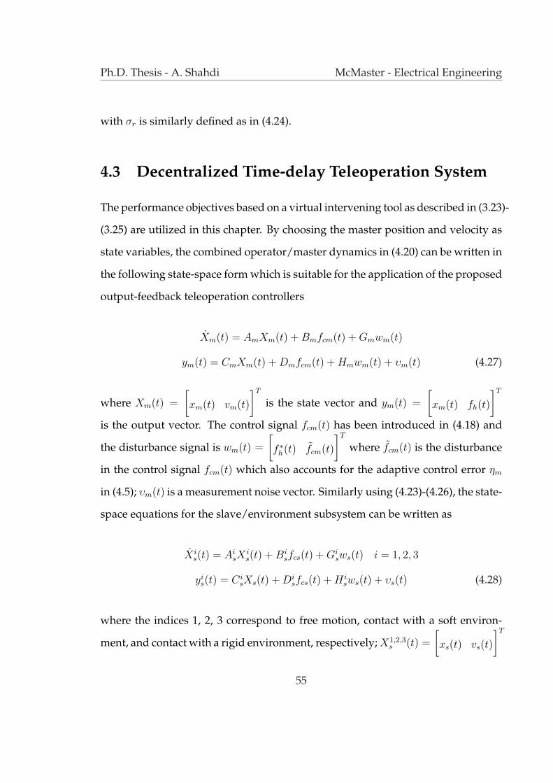
Ph.D. Thesis - A. Shahdi McMaster - Electrical Engineering
with σr is similarly defined as in (4.24).
4.3 Decentralized Time-delay Teleoperation System
The performance objectives based on a virtual intervening tool as described in (3.23)-
(3.25) are utilized in this chapter. By choosing the master position and velocity as
state variables, the combined operator/master dynamics in (4.20) can be written in
the following state-space form which is suitable for the application of the proposed
output-feedback teleoperation controllers
Xm(t) = AmXm(t) + Bmfcm(t) + Gmwm(t)
ym(t) = CmXm(t) + Dmfcm(t) + Hmwm(t) + υm(t) (4.27)
where Xm(t) =
[xm(t) vm(t)
]T
is the state vector and ym(t) =
[xm(t) fh(t)
]T
is the output vector. The control signal fcm(t) has been introduced in (4.18) and
the disturbance signal is wm(t) =
[f ∗h(t) fcm(t)
]T
where fcm(t) is the disturbance
in the control signal fcm(t) which also accounts for the adaptive control error ηm
in (4.5); υm(t) is a measurement noise vector. Similarly using (4.23)-(4.26), the state-
space equations for the slave/environment subsystem can be written as
X is(t) = Ai
sXis(t) + Bi
sfcs(t) + Gisws(t) i = 1, 2, 3
yis(t) = Ci
sXs(t) + Disfcs(t) + H i
sws(t) + υs(t) (4.28)
where the indices 1, 2, 3 correspond to free motion, contact with a soft environ-
ment, and contact with a rigid environment, respectively; X1,2,3s (t) =
[xs(t) vs(t)
]T
55

Ph.D. Thesis - A. Shahdi McMaster - Electrical Engineering
and ys(t) =
[xs(t) fe(t)
]is the measurement vector. The control signal is fcs(t)
and the disturbance vector is ws(t) =
[f ∗e (t) fcs(t)
]T
. The desired tool dynamics
in (3.23) can also be written as
Xt(t) = AtXt(t) + Btut(t)
yt(t) = Xt(t) (4.29)
where Xt(t) =
[xt(t) vt(t)
]T
, ut(t) =
[fh(t) fe(t)
]T
and yt(t) = Xt(t). The state-
space matrices for the operator/master, slave/environment and tool dynamics are
all presented in Appendix A.
Systematic output-feedback control schemes such as the LQG control are es-
sentially centralized and must be stationed either at the master or slave site. For
example, the top part of Fig. 4.2(a) depicts the case in which the centralized con-
troller is placed at the master site hence having access to delay-free master and de-
layed slave position and force measurements. Similarly, the master control signal
is delay-free whereas the slave control command is delayed because of its trans-
mission over the communication channel. The bottom part of Fig. 4.2(a) displays
the teleoperation system with the controller at the slave end. A centralized tele-
operation architecture lends itself to the model-based delay-reduction and output-
feedback control method proposed in [2]. The drawback, however, is that such
architecture would introduce extra round-trip delay in the control loop, negatively
affecting the trade-off between the performance and robust stability. For instance
in the case of a centralized controller at the master site, local measurements at the
slave site must undergo a round-trip delay before being used in the control of the
56

Ph.D. Thesis - A. Shahdi McMaster - Electrical Engineering
Figure 4.2: Conceptual representation of the proposed model-predictive decen-tralized teleoperation controller: (a) Centralized teleoperation control at masteror slave side; (b) Decentralized sub-controller design; (c) Decentralized controllerimplementation.
slave robot.
To improve the performance-robustness trade-off of the delay reduction-based
teleoperation controller in [2], a decentralized control architecture utilizing the
proposed delay reduction technique is introduced here. The design concept is
demonstrated in Fig. 4.2(b-c) in which the problem is divided into two central-
ized sub-controllers, one at the master and the other at the slave site. Each control
57

Ph.D. Thesis - A. Shahdi McMaster - Electrical Engineering
station has access to delay-free local and delayed remote position and force mea-
surements. However unlike the case of the centralized controllers in Fig. 4.2(a),
both control outputs of these sub-controllers are assumed to be delay-free. From
the two control signals that are produced by each station, only the local control
commands are used for the control of the master and slave robots as shown in
Fig. 4.2(c), i.e.
fcm(t) = u11(t) , fcs(t) = u2
2(t). (4.30)
The remaining two control signals, u12(t) and u2
1(t), are local estimates of the re-
mote control forces at the master and slave sites and are not being used in the
implementation. It should be pointed out that the stability of the closed-loop sys-
tem with each individual sub-controller in Fig. 4.2(b) provides no guarantee of the
stability of the actual system in Fig. 4.2(c). This will be thoroughly investigated
later in this chapter.
The change in the slave/enviroment dynamics due to rigid contact and param-
eter variations due to soft contact can be handled within a multi-model control
framework in which mode-based controllers are designed for different phases of
the operation. In this strategy, dedicated controllers are designed for each mode
of the operation and switching between controllers occurs according to the iden-
tified mode. Similar technique has been successfully employed in our previous
contributions in [119, 1, 2] to handle the environment uncertainties.
58

Ph.D. Thesis - A. Shahdi McMaster - Electrical Engineering
4.3.1 Free motion/soft contact
The states of the system are obtained by combining the master, slave and tool sub-
system dynamics. For the cases of free motion/soft contact, system states are de-
fined as follows
X(t) =
[αpXs(t)−Xm(t) Xm(t)−Xt(t) Xt(t)
]T
(4.31)
where Xm(t), Xs(t), and Xt(t) have been introduced in (4.27), (4.28) and (4.29),
and αf and αp have been defined in (3.23) and (3.24). The position tracking errors
between the master and slave, and the master and virtual tool are included in
the state vector. An application of output-feedback LQG control to regulate these
tracking errors to zero would enforce the transparency objectives defined in (3.23)-
(3.25). The evolution of the states is governed by
X(t) = AX(t) + Bu(t) + Gw(t)
u(t) =
[fcm(t) fcs(t)
]T
w(t) =
[f ∗h(t) f ∗e (t) fcm(t) fcs(t)
]T
. (4.32)
It is straightforward to obtain the system matrices, A, B, and G from Am, Bm, Cm,
Dm, Gm, Hm, As, Bs, Cs, Ds, Gs, Hs, At, and Bt. These matrices are presented in
Appendix B. The measurement vectors are
y1(t) =
[ym(t) ys(t− d) yt(t− d)
]T
y2(t) =
[ym(t− d) ys(t) yt(t− d)
]T
(4.33)
59
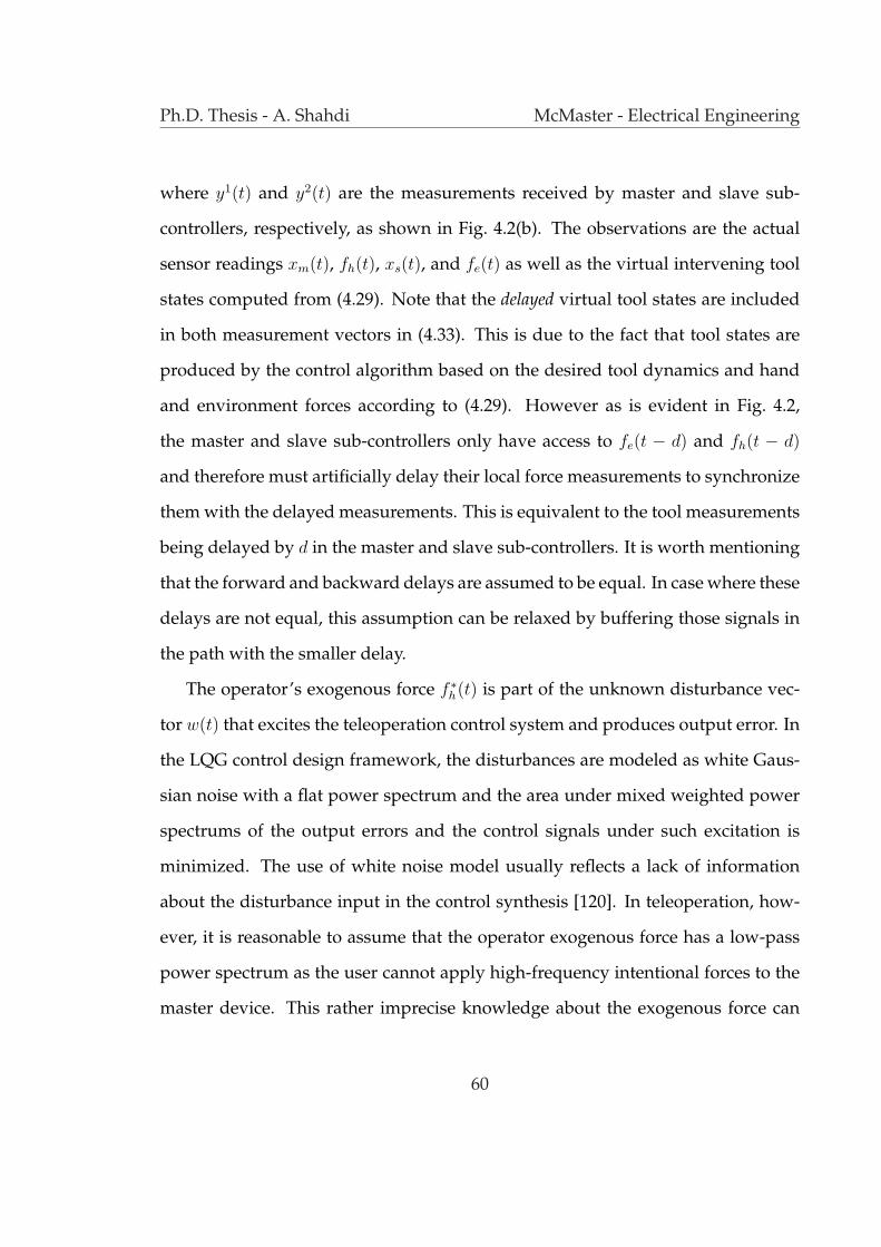
Ph.D. Thesis - A. Shahdi McMaster - Electrical Engineering
where y1(t) and y2(t) are the measurements received by master and slave sub-
controllers, respectively, as shown in Fig. 4.2(b). The observations are the actual
sensor readings xm(t), fh(t), xs(t), and fe(t) as well as the virtual intervening tool
states computed from (4.29). Note that the delayed virtual tool states are included
in both measurement vectors in (4.33). This is due to the fact that tool states are
produced by the control algorithm based on the desired tool dynamics and hand
and environment forces according to (4.29). However as is evident in Fig. 4.2,
the master and slave sub-controllers only have access to fe(t − d) and fh(t − d)
and therefore must artificially delay their local force measurements to synchronize
them with the delayed measurements. This is equivalent to the tool measurements
being delayed by d in the master and slave sub-controllers. It is worth mentioning
that the forward and backward delays are assumed to be equal. In case where these
delays are not equal, this assumption can be relaxed by buffering those signals in
the path with the smaller delay.
The operator’s exogenous force f ∗h(t) is part of the unknown disturbance vec-
tor w(t) that excites the teleoperation control system and produces output error. In
the LQG control design framework, the disturbances are modeled as white Gaus-
sian noise with a flat power spectrum and the area under mixed weighted power
spectrums of the output errors and the control signals under such excitation is
minimized. The use of white noise model usually reflects a lack of information
about the disturbance input in the control synthesis [120]. In teleoperation, how-
ever, it is reasonable to assume that the operator exogenous force has a low-pass
power spectrum as the user cannot apply high-frequency intentional forces to the
master device. This rather imprecise knowledge about the exogenous force can
60
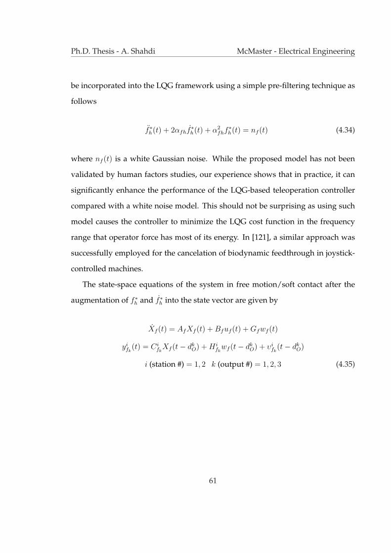
Ph.D. Thesis - A. Shahdi McMaster - Electrical Engineering
be incorporated into the LQG framework using a simple pre-filtering technique as
follows
f ∗h(t) + 2αfhf∗h(t) + α2
fhf∗h(t) = nf (t) (4.34)
where nf (t) is a white Gaussian noise. While the proposed model has not been
validated by human factors studies, our experience shows that in practice, it can
significantly enhance the performance of the LQG-based teleoperation controller
compared with a white noise model. This should not be surprising as using such
model causes the controller to minimize the LQG cost function in the frequency
range that operator force has most of its energy. In [121], a similar approach was
successfully employed for the cancelation of biodynamic feedthrough in joystick-
controlled machines.
The state-space equations of the system in free motion/soft contact after the
augmentation of f ∗h and f ∗h into the state vector are given by
Xf (t) = AfXf (t) + Bfuf (t) + Gfwf (t)
yifk
(t) = Cifk
Xf (t− dkO) + H i
fkwf (t− dk
O) + υifk
(t− dkO)
i (station #) = 1, 2 k (output #) = 1, 2, 3 (4.35)
61

Ph.D. Thesis - A. Shahdi McMaster - Electrical Engineering
and
Xf (t) =
[X(t) f ∗h(t) f ∗h(t)
]T
y1f (t) = y1(t) =
[ym(t) ys(t− d) yt(t− d)
]T
y2f (t) = y2(t) =
[ym(t− d) ys(t) yt(t− d)
]T
uf (t) = u(t) =
[fcm(t) fcs(t)
]T
wf (t) =
[nf (t) f ∗e (t) fcm(t) fcs(t)
]T
υ1f (t) = υ2
f (t) =
[υm(t) υs(t) 0
]T
(4.36)
where dkO is the delay in the k’th output channel. The reader is referred to Ap-
pendix B for the state-space matrices of the system dynamics in free motion/soft
contact.
4.3.2 Rigid contact
When the slave is in rigid contact, its dynamics are governed by (4.25)-(4.26). In
this case, the vector of states including the master and slave subsystems is chosen
as
X(t) = [xm(t)− αpxs(t) vm(t) xs(t) fe(t) αf fe(t)− fh(t)]T (4.37)
62

Ph.D. Thesis - A. Shahdi McMaster - Electrical Engineering
and the measurement vectors are
y1(t) =
[ym(t) xs(t− d) fe(t− d)
]T
y2(t) =
[ym(t− d) xs(t) fe(t)
]T
. (4.38)
In (4.37), fe(t) and fh(t) are generated by passing force sensor measurements fe(t)
and fh(t) through the following first-order filters with poles at −β
˙fe(t) + βfe(t) = βfcs, (4.39)
˙fh(t) + βfh(t) = βfh. (4.40)
These first-order filters convert the algebraic equations of the rigid contact in (4.25)-
(4.26) to dynamic-type equations involving new states fe and αf fe − fh, enabling
the application of the LQG control. The effect of the design parameter β is similar
to the one described for the parameter c in (4.6). The dynamics of filtered force
tracking error αf fe − fh can be easily derived from the filter equations above
αf˙fe(t)− ˙fh(t) = −β(αf fe(t)− fh(t)) + αfβfcs − βfh (4.41)
and fh can be written in terms of the states and inputs. Assuming to be almost
constant, the slave position in rigid contact, xs(t), is modeled by
xs(t) = wxs(t) (4.42)
63

Ph.D. Thesis - A. Shahdi McMaster - Electrical Engineering
where wxs(t) is white Gaussian noise. The steps for incorporating the operator’s
exogenous force f ∗h(t) into the system states are similar to those in the previous
case and will not be repeated here. The dynamics of the augmented system can be
expressed by the following equations
Xr(t) = ArXr(t) + Brur(t) + Grwr(t)
yirk
(t) = Cirk
Xr(t− dkO) +
∑nI=2j=1 Di
rkjuj
rj(t− dkO) +
H irk
wr(t− dkO) + υi
rk(t− dk
O) (4.43)
with
Xr(t) =
[X(t) f ∗h(t) f ∗h(t)
]T
y1r(t) = y1(t) =
[ym(t) ys(t− d) fe(t− d)
]
y2r(t) = y2(t) =
[ym(t− d) ys(t) fe(t)
]
ur(t) =
[fcm(t) fcs(t)
]T
wr(t) =
[nf (t) fcm(t) fcs(t) wxs(t)
]
υ1r(t) = υ2
r(t) =
[υm(t) 0
](4.44)
where nI is the number of inputs. The state-space matrices in rigid contact are
given in Appendix B.
64
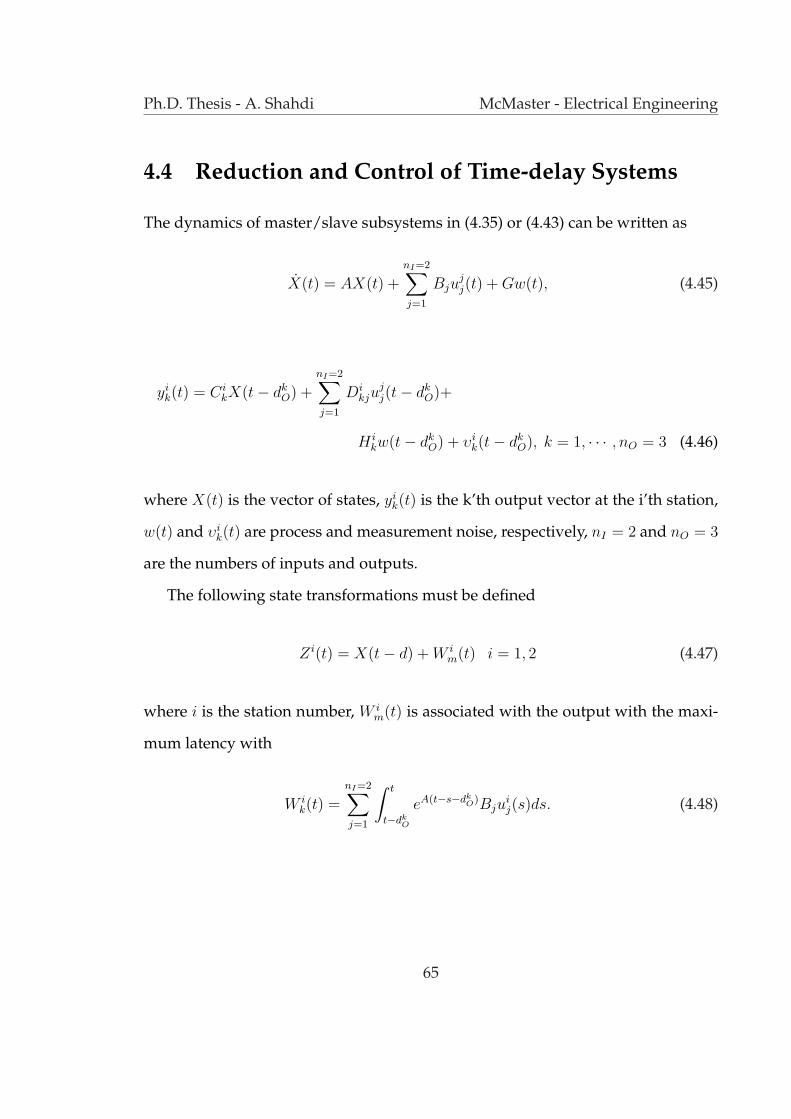
Ph.D. Thesis - A. Shahdi McMaster - Electrical Engineering
4.4 Reduction and Control of Time-delay Systems
The dynamics of master/slave subsystems in (4.35) or (4.43) can be written as
X(t) = AX(t) +
nI=2∑j=1
Bjujj(t) + Gw(t), (4.45)
yik(t) = C i
kX(t− dkO) +
nI=2∑j=1
Dikju
jj(t− dk
O)+
H ikw(t− dk
O) + υik(t− dk
O), k = 1, · · · , nO = 3 (4.46)
where X(t) is the vector of states, yik(t) is the k’th output vector at the i’th station,
w(t) and υik(t) are process and measurement noise, respectively, nI = 2 and nO = 3
are the numbers of inputs and outputs.
The following state transformations must be defined
Zi(t) = X(t− d) + W im(t) i = 1, 2 (4.47)
where i is the station number, W im(t) is associated with the output with the maxi-
mum latency with
W ik(t) =
nI=2∑j=1
∫ t
t−dkO
eA(t−s−dkO)Bju
ij(s)ds. (4.48)
65

Ph.D. Thesis - A. Shahdi McMaster - Electrical Engineering
Taking the time derivative of (4.47) and replacing X(t− d) from (4.45) yield
Z1(t) = AzZ1(t) + Bz1u
11(t) + Bz2u
21(t)
−B2u12(t− d)− u2
2(t− d)+ Gw(t− d)
Z2(t) = AzZ2(t) + Bz1u
21(t) + Bz2u
22(t)
−B1u21(t− d)− u1
1(t− d)+ Gw(t− d), (4.49)
Az = A, Bz =[e−AdB1, e−AdB2
]. (4.50)
For the system described in (4.45), X(t− d) can be written in terms of X(t− dkO)
using standard results from the linear systems theory as follows [122]
X(t− d) = e−AdmkO X(t− dk
O)−nI=2∑j=1
∫ t−dkO
t−d
eA(t−s−d)Bjujj(s)ds
−∫ dmk
o
0
e−AsGw(t− d + s)ds (4.51)
where dmkO = d − dk
O. Replacing X(t − d) in (4.47) from (4.51) for i = 1, and then
multiplying both sides from left by C1ke
Admko , one may write
C1ke
AdmkO Z1(t) = C1
kX(t− dkO)− C1
k
∫ 0
−dmko
e−AsGw(t + s)ds
+ C1kW
1k +
∫ t−dkO
t−d
C1ke
A(t−s−dkO)B2(u
12(s)− u2
2(s))ds. (4.52)
It can be shown that in the case of teleoperation system, the last term in (4.52) is
always zero for both free motion/soft contact and rigid contact cases and for every
66
Ph.D. Thesis - A. Shahdi McMaster - Electrical Engineering
k, i.e. k = 1, 2, 3. Considering the first station output vectors in (4.33) and (4.38) for
free motion/soft contact and rigid contact cases, the following is true
dkO = d , k = 2, 3. (4.53)
Therefore, the last term in (4.52) is equal to zero for k = 2, 3 due to the equality of
the integral bounds. For k = 1, the integral term represents an effect of the second
input, fcs, on the first output, ym. Since the slave control action has no impact
on the master outputs, the last term in (4.52) will also be equal to zero for k = 1.
Similar results can be obtained for the second station by replacing X(t−d) in (4.47)
from (4.51) for i = 2.
A new output vector for the k’th channel at station i, yizk(t), is defined as
yizk(t) = Ci
keAdmk
o Zi(t) + H ikw(t− dk
O)
+ υik(t− dk
O) + C ik
∫ 0
−dmko
e−AsGw(t + s)ds (4.54)
or equivalently,
yiz(t) = Ci
zZi(t) + υi
z(t) i = 1, 2 (4.55)
with
Ciz =
[(Ci
1eAdm1
o )T (Ci2e
Adm2o )T · · · (Ci
noeAdmno
o )T
]T
. (4.56)
67

Ph.D. Thesis - A. Shahdi McMaster - Electrical Engineering
Using (4.46) and (4.52), yizk(t) in (4.54) can be calculated from
yizk(t) = yi
k(t)−nI=2∑j=1
Dikju
jj(t− dk
O) + CikW
ik(t). (4.57)
This completes the derivation of the reduced system dynamics and the output
equations in (4.49) and (4.55). The calculation of the new observation vectors
in (4.57) involves the computation of W ik(t)’s that can be obtained from
W ik(t) = AW i
k(t) +
nI=2∑j=1
e−AdkOBju
ij(t)−
nI=2∑j=1
Bjuij(t− dk
O),
yiwk(t) = Ci
kWik(t), W i
k(0) = 0. (4.58)
Since the states of the system are not directly available, an observer/controller
pair can be designed to control the reduced system based on the new measure-
ments. The following theorem is needed for the control of the reduced system.
Theorem 4.1: The reduced system in (4.49) and (4.55) is stabilizable and detectable
if the original system in (4.45) is stabilizable and detectable.
Proof : See Appendix C for the proof.
At each station i, ui1 and ui
2 are calculated using the local measurement accord-
ing to the LQG control, to minimize the following cost function as T →∞ [123]
J i(u) =1
TE
∫ T
0
[Zi(t)T QZi(t) + ui1(t)
T R1ui1(t) + ui
2(t)T R2u
i2(t)]dt (4.59)
68

Ph.D. Thesis - A. Shahdi McMaster - Electrical Engineering
where E. denotes the expected value, and Q ≥ 0, R1 > 0 and R2 > 0.
The solution to (4.59) is a combination of a constant state-feedback gain pro-
duced by solving the corresponding deterministic Linear Quadratic (LQ) control
and a Kalman filter state estimator for the ith station, i.e.
ui1(t) = −K1Z
i(t), ui2(t) = −K2Z
i(t). (4.60)
The feedback gain K1 and K2 are given by
K1 = R−11 B1
zTS, K2 = R−1
2 B2z
TS (4.61)
and S is the solution to the following Continuous-time Algebraic Riccati Equation
(CARE)
ATz S + SAz − S
(B1
zR−11 B1
zT
+ B2zR
−12 B2
zT)
S + Q = 0. (4.62)
The state estimate at the ith station, Zi(t), is the output of a Kalman filter with the
following dynamics
˙Zi(t) = AzZ
i(t) + B1zu
i1(t) + B2
zui2(t) + Li
[yi
z(t)− CizZ
i(t)]. (4.63)
The Kalman filter gain Li is computed as follows [124]
Li = P iCiz
TΠi−1 (4.64)
69

Ph.D. Thesis - A. Shahdi McMaster - Electrical Engineering
where P i is the solution to the following CARE
P iATz − P iCi
z
TΠi−1
CizP
i + AzPi + W = 0 (4.65)
with
W = EGw(t)w(t)T GT
(4.66)
and
Πi = Eυi
z(t)υiz(t)
T
(4.67)
being the covariances of the process and measurement noise, respectively. Cer-
tain conditions must be satisfied for the existence of a solution to the local LQG
problems. These include the stabilizability of pair (Az, Bz) and detectability of pair
(Ciz, Az) among others. It can be shown that the teleoperation system satisfies all
necessary requirements. Furthermore according to Theorem 4.1, the stabilizability
and detectability are preserved under the proposed state/output transformations.
To achieve the teleoperation performance objectives, the Q and R matrices for
free motion/soft contact are selected as
Xf (t)T QfXf (t) = q1(αpxs(t)− xm(t))2 + q2(xm(t)− xt(t))
2 (4.68)
with q1 > 0 and q2 > 0. Similarly for rigid contact,
Xr(t)T QrXr(t) = q1(xm(t)− αpxs(t))
2 + q2(αf fe(t)− fh(t))2. (4.69)
The quadratic terms in (4.68) and (4.69) involve position and force tracking er-
rors at concurrent sample times. Therefore despite the presence of the delay, the
70
Ph.D. Thesis - A. Shahdi McMaster - Electrical Engineering
controller attempts to produce non-delayed position and force tracking, as well as
tool impedance shaping. Also, the matrices Qf and Qr are positive semi-definite
as opposed to positive definite. This is critical for the design of the teleoperation
controller since the system must be allowed to move freely. Therefore, only the
tracking errors of interest are penalized in (4.59) and the gains corresponding to
the rest of the states in the Q’s are set to zero. The LQG control synthesis in (4.59)
is conducted using the transformed states Zi(t) rather than the original states. Note
that
e−AdX(t) = X(t− d) +
nI∑j=1
∫ t
t−d
eA(t−s−d)Bjuij(s)ds ≈ Zi(t). (4.70)
Therefore, proper scaling for matrices Qf add Qr may be obtained by considering
X(t)T QX(t) ≈ Zi(t)T eAT dQeAdZi(t). (4.71)
Finally, it is also worth mentioning that the derivatives of the control signals in (4.60)
needed in the adaptive nonlinear controllers in Section 2 can be obtained by
ui1(t) = −K1
˙Zi(t), ui
2(t) = −K2˙Zi(t) (4.72)
where ˙Zi(t) is calculated from the dynamics of the Kalman filters in (4.63). Local
and remote position and force measurements are utilized at the master and slave
sites to generate these dynamics.
71

Ph.D. Thesis - A. Shahdi McMaster - Electrical Engineering
4.4.1 Closed-loop Stability Analysis
After replacing the inputs from (4.60) in the dynamic equations of the reduced
system in (4.49), one may obtain
Z1(t)
Z2(t)
=
Az 0
0 Az
Z1(t)
Z2(t)
+
−BzK 0
0 −BzK
·
Z1(t)
Z2(t)
+
B2K2 −B2K2
−B1K1 B1K1
Z1(t− d)
Z2(t− d)
. (4.73)
Combining the reduced system dynamics in (4.73) with observer dynamics in (4.63)
results in the following closed-loop dynamics
Z(t)
˙Z(t)
=
Az −BzK 0 BzK 0
0 Az −BzK 0 BzK
0 0 Az − L1C1z 0
0 0 0 Az − L2C2z
Z(t)
Z(t)
+
B2K2 −B2K2 −B2K2 B2K2
−B1K1 B1K1 B1K1 −B1K1
B2K2 −B2K2 −B2K2 B2K2
−B1K1 B1K1 B1K1 −B1K1
Z(t− d)
Z(t− d)
(4.74)
72

Ph.D. Thesis - A. Shahdi McMaster - Electrical Engineering
where Z(t) = Z(t) − Z(t), Z(t) =
[Z1(t) Z2(t)
]T
and Z(t) =
[Z1(t) Z2(t)
]T
.
It can be seen that the closed-loop dynamics are in the following general state-
delayed form
x(t) = A0x(t) + A1x(t− τ) (4.75)
with τ = d. It is important to note that unlike in the case of the centralized delay
reduction based controller in [2], the application of the decentralized delay reduc-
tion and control would not yield a completely delay-free system. The state delayed
perturbation term A1x(t − d) appearing in (4.74) is due to the difference between
the actual control signal and their remote estimated counterparts in (4.49). Since
the delay reduction and control process have utilized the model and delay infor-
mation to provide an embedded predictive control element, the effect of the extra
state-delay perturbation term on the system stability and performance is expected
to be small compared with the case where the controller has no built-in predic-
tor. In fact if u11 = u2
1 and u22 = u1
2, this perturbation term would vanish from the
closed-loop dynamics.
The closed-loop stability of a system in the form of (4.75) can be examined using
the following theorem.
Theorem [Frequency-Sweeping Test]: For the state-delayed system in (4.75), pro-
vided that A0 is stable, the closed-loop stability is guaranteed for a maximum delay
derived from
τ = mini
(θi
ωi
), ∀λi(jωiI − A0, A1) = e−jθi (4.76)
where λ(A, B) denotes the generalized eigenvalues of matrices A and B.
Proof: See [22].
73

Ph.D. Thesis - A. Shahdi McMaster - Electrical Engineering
Note that the stability of matrix A0 in equation (4.74) is guaranteed owing to its
upper triangular structure and the fact that the diagonal elements Az −BzK, Az −L1C1
z , and Az − L2C2z obtained from the LQ and Kalman filter design procedures
have all of their eigenvalues in the left half of the complex plane. Provided that the
maximum delay calculated from (4.76) is greater than the nominal delay assumed
in the design, the stability of the reduced closed-loop system is guaranteed.
Theorem: If the reduced system is stabilized through a decentralized output-feedback
controller, the original delayed system will also become stable.
Proof : The stability of the reduced system/observer implies that the reduced states
Zi(t) and their estimates Zi(t) remain bounded in the presence of bounded dis-
turbance and noise. Hence, the control signal ui(t) which is given by (4.60) is also
bounded. From (4.47), the original system states can be written as
X(t− d) = Zi(t)−W im(t) (4.77)
where
W im(t) =
nI∑j=1
∫ t
t−d
eA(t−s−d)Bjuij(s)ds (4.78)
and W im(t) is bounded as a result of boundedness of ui(t). Since both terms on
the right hand side of (4.77) are bounded, X(t − d) and consequently X(t) are
also bounded. Therefore the pair of observer/controller for the reduced system
stabilizes the original system as well. Note that if zero is an asymptotically stable
point for the reduced states Zi(t), then it would also be an asymptotically stable
74

Ph.D. Thesis - A. Shahdi McMaster - Electrical Engineering
Figure 4.3: Multi-model decentralized controller for time-delay teleoperation.
point for the original states X(t). Q.E.D.
A schematic of the proposed multi-model LQG-based teleoperation control sys-
tem is displayed in Fig. 4.3. The sensor measurements are the master and slave
positions as well as the hand and environment forces. Delayed hand and environ-
ment force signals are used to generate delayed virtual tool position and velocity
at each station. These synthesized and actual observations enter the mode-based
LQG controller blocks at the master and slave sites which produce the mode-based
control signals. The switching logic, located at the slave side, uses the sensor mea-
surements to identify the mode of operation and sends the result to the controller
at the master side. This information is utilized in selecting the pair of control sig-
nals to be used by the master and slave actuators.
75

Ph.D. Thesis - A. Shahdi McMaster - Electrical Engineering
The disturbance signal f ∗h(t) is the cause of motion in teleoperation. The LQG
design framework attempts to minimize the effect of the stochastic perturbations
on the tracking errors, and as such coordinates the motions of master and slave
robots. For example in free motion/soft contact, the disturbances drive the virtual
tool dynamics in (4.29) which are not controllable by the control signals. Therefore,
the controller must move the master and slave in response to operator’s exogenous
force such that the transparency objectives are achieved, i.e. the tracking errors
among master, slave and tool are reduced.
Nominal model parameters of the operator, master robot, slave robot, and en-
vironment dynamics are used by the mode-based controllers. While the adaptive
nonlinear controller in (4.2)-(4.4) renders the master and slave parameters constant,
the operator and environment dynamics are usually unknown and time-varying.
A deviation from the nominal parameters can degrade the system performance
and even cause instability. Tightening the control loops through the adjustment
of the LQ controller parameters could improve the performance by reducing the
tracking errors and increasing the speed of the system response. However, this
would be achieved at the expense of reduced stability margins and potential insta-
bility due to parametric uncertainty.
A careful selection of switching strategy can yield a smooth contact transition
behavior. While the stability of mode-based controllers is guaranteed by the LQG
design, it is difficult to prove the stability of the teleoperation system in the pres-
ence of control switching. This remains beyond the scope of the present thesis and
will be a subject of future research. Interested reader is referred to [125] for an
example of stability analysis of a gain-switching teleoperation controller.
76
Ph.D. Thesis - A. Shahdi McMaster - Electrical Engineering
As in [2], the control design can be extended to the case in which the delays
in the forward and return paths of the master/slave communication link are dif-
ferent. The round-trip delay can be easily estimated by attaching time stamps to
data packets. The one-way delays, if equal, are half of the round-trip delay. Oth-
erwise, the master and slave computer clocks can be synchronized to an external
universal time reference, e.g. Universal Coordinated Time, via GPS or special radio
signals [126]. Once the computer clocks are synchronized, the data packets can be
again time-stamped for delay estimation. Variable delays can be accommodated
by adding buffers at the master and slave ends and delaying the signals to a max-
imum a priori known delay. The controller can then be designed for this constant
delay.
4.5 Performance and Robust Stability Analysis for Single-
axis Teleoperation
The proposed decentralized multi-model LQG control scheme is applied to a lin-
ear single-axis bilateral teleoperation system involving two similar masses. Since
the master and slave dynamics are already linear and known, the adaptive non-
linear impedance controller is not needed in this example. Throughout the rest
of the chapter, the delay values correspond to a round-trip communication unless
otherwise noted. It is assumed that the operator manipulates the slave robot in
free motion and in contact with a rigid environment and hence two mode-based
controllers are designed.
The system parameters in Table 4.1 are based on the experimental setup which
77

Ph.D. Thesis - A. Shahdi McMaster - Electrical Engineering
System ParametersMaster mm = 1.0 kg bm = 2.0 N.s/m km = 0 N/mSlave ms = 1.0 kg bs = 2.0 N.s/m ks = 0 N/mVirtual Tool mt = 1.0 kg bt = 2.0 N.s/m kt = 0 N/mArm mh = 2.0 kg bh = 2.0 N.s/m kh = 30.0 N/mEnvironment me = 0 kg be = 0 N.s/m ke = 0 N/mOther αf = 1 αp = 1 αfh = 0.01 rad/s β = 0.8 rad/s
LQG Controller ParametersFree Motion
q1 = q2 = 4× 10⁵ m−2
R = diag(0.1 N−2, 0.1 N−2
)EwfwT
f = diag(104 N2/s4, 200 N2, 10−3 N2, 10−3 N2
)
Rigid Contactq1 = 103 m−2 q2 = 5.0 N−2
R = diag(0.001 N−2, 0.001 N−2
)Ewrw
Tr = diag
(10 N2/s4, 10−4 N2, 10−6 N2, 10−5 m2/s2
)
Table 4.1: The system and the proposed decentralized controller parameters.
will be introduced in the next section. Typical values have been chosen for the arm
mass, damping and stiffness. The LQG control parameters are also presented in
this table. Among these, the values of measurement and disturbance noise powers
were initially selected based on sensor and actuator specifications as well as a typ-
ical level of operator hand force and later refined based on simulation and experi-
mental results. The Q and R in the LQG synthesis play a pivotal role in achieving
a balance between performance and stability. A large Q and small R would gen-
erally yield faster poles, small tracking errors and enhanced performance at the
expense of reduced robustness. These parameters have been manually tuned to
strike a balance between these requirements.
In the forthcoming analysis, the stability margins and tracking performance
of the decentralized controller with the above design parameters are numerically
78
Ph.D. Thesis - A. Shahdi McMaster - Electrical Engineering
calculated. The results are compared with those obtained from the centralized con-
troller proposed in [2]. To allow for a fair comparison, the same set of parameters
were employed in the design of both controllers.
4.5.1 Robust stability analysis w.r.t parametric uncertainty
The robustness of the proposed controller with respect to parametric uncertainty
can be investigated using classical linear analysis tools such as the Nyquist theo-
rem. Among the model parameters, those of environment and operator are subject
to uncertainty. In Fig. 4.4, the robustness of the mode-based controllers with re-
spect to variations in individual parameters and as a function of communication
latency is examined for both the decentralized and the centralized controllers. The
environment stiffness in the design of the free-motion controller is set to 0 N/m.
The robustness of the controllers w.r.t. uncertainty in the environment stiffness
is examined in Fig. 4.4(a) where the maximum stiffness for stability decreases by
the amount of time delay from more than 4500 N/m for round-trip delays less than
20 ms to about 250 N/m for a delay of 250 ms. It can be seen that the decentralized
controller exhibits a higher stability margin. In fact, this trend is evident in all other
diagrams for free motion. In Fig. 4.4(c), the robustness of the free motion controller
with respect to uncertainty in the operator’s arm stiffness is demonstrated. The
nominal value of stiffness used in the controller design is 30 N/m. In Figs. 4.4(b)
and 4.4(d), the sensitivity of the free-motion and rigid-contact controllers with re-
spect to variations in the operator’s arm mass are examined where the nominal
value of the arm mass used in the design is 2.0 kg according to Table 4.1. It can be
seen that the arm mass stability margins in rigid contact are almost the same for
79

Ph.D. Thesis - A. Shahdi McMaster - Electrical Engineering
Figure 4.4: Robust stability analysis results in free motion: (a), (b) and (c), and inrigid contact: (d), as a function of time delay.
centralized and decentralized controllers. This trend is observed in the robustness
of the rigid contact controllers with respect to changes in other parameters as well.
The robust stability analysis was also performed for simultaneous variations in
two system parameters at a fixed delay of 125 ms, the results of which are given in
Fig. 4.5. To obtain these graphs, one parameter was varied in fixed size steps while
the stability bound on the second parameter was computed using the Nyquist cri-
terion. Again it is evident that the decentralized controller enjoys higher or at least
equal stability margins to those of the centralized controller.
80
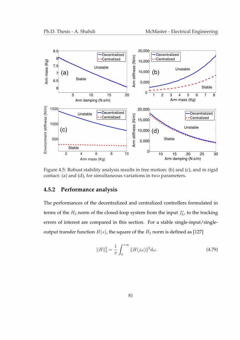
Ph.D. Thesis - A. Shahdi McMaster - Electrical Engineering
Figure 4.5: Robust stability analysis results in free motion: (b) and (c), and in rigidcontact: (a) and (d), for simultaneous variations in two parameters.
4.5.2 Performance analysis
The performances of the decentralized and centralized controllers formulated in
terms of the H2 norm of the closed-loop system from the input f ∗h , to the tracking
errors of interest are compared in this section. For a stable single-input/single-
output transfer function H(s), the square of the H2 norm is defined as [127]
‖H‖22 =
1
π
∫ +∞
0
‖H(jω)‖2dω. (4.79)
81
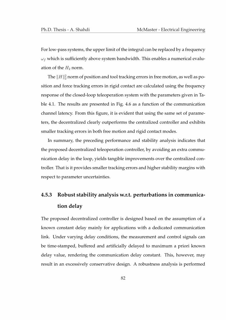
Ph.D. Thesis - A. Shahdi McMaster - Electrical Engineering
For low-pass systems, the upper limit of the integral can be replaced by a frequency
ωf which is sufficiently above system bandwidth. This enables a numerical evalu-
ation of the H2 norm.
The ‖H‖22 norm of position and tool tracking errors in free motion, as well as po-
sition and force tracking errors in rigid contact are calculated using the frequency
response of the closed-loop teleoperation system with the parameters given in Ta-
ble 4.1. The results are presented in Fig. 4.6 as a function of the communication
channel latency. From this figure, it is evident that using the same set of parame-
ters, the decentralized clearly outperforms the centralized controller and exhibits
smaller tracking errors in both free motion and rigid contact modes.
In summary, the preceding performance and stability analysis indicates that
the proposed decentralized teleoperation controller, by avoiding an extra commu-
nication delay in the loop, yields tangible improvements over the centralized con-
troller. That is it provides smaller tracking errors and higher stability margins with
respect to parameter uncertainties.
4.5.3 Robust stability analysis w.r.t. perturbations in communica-
tion delay
The proposed decentralized controller is designed based on the assumption of a
known constant delay mainly for applications with a dedicated communication
link. Under varying delay conditions, the measurement and control signals can
be time-stamped, buffered and artificially delayed to maximum a priori known
delay value, rendering the communication delay constant. This, however, may
result in an excessively conservative design. A robustness analysis is performed
82
Ph.D. Thesis - A. Shahdi McMaster - Electrical Engineering
Figure 4.6: ‖H‖22 for the closed-loop system from f ∗h to (a) position tracking error
in free motion, (b) tool tracking error in free motion, (c) position tracking error inrigid contact, and (d) force tracking error in rigid contact.
to determine the maximum allowable variations in the delay to maintain the sys-
tem stability. The value of the delay is assumed to be unknown and constant but
different from that used in the design.
A model of the closed-loop decentralized teleoperation control system subject
to uncertainty in communication delay is depicted in Fig. 4.7. The actual commu-
nication channel delay is equal to d + ∆d where d is the nominal value used in the
design and ∆d is a delay perturbation. The stability margins, i.e. the maximum
and minimum ∆d for which the system remains stable, can be found using the
83

Ph.D. Thesis - A. Shahdi McMaster - Electrical Engineering
Figure 4.7: Closed-loop decentralized teleoperation control subject to uncertaintyin communication delay.
characteristic equation of the closed-loop system defined by
p (s, ∆d) = det (I −∆(s)G(s)) = 0 (4.80)
where matrix G is the nominal transfer function for the MIMO system without the
perturbation shown in Fig. 4.7 and the matrix
∆ =
e−s∆d 0
0 e−s∆d
(4.81)
84

Ph.D. Thesis - A. Shahdi McMaster - Electrical Engineering
Figure 4.8: Maximum/minimun allowable time-delay variations to maintain sta-bility.
is the perturbation to the communication channel delay. Since the proposed con-
troller stabilizes the non-perturbed system, the stability margins can be found
by sweeping ∆d in the negative and positive directions and finding the first two
points such that
∃ω > 0, p (jω, ∆d) = 0. (4.82)
Using the system and controller parameters in Table 4.1, the margins of stability
for the decentralized controller in free motion are calculated and the results are
plotted in Fig. 4.8. It can be seen from this figure that the system is stable for
almost twice the nominal delay of 250 ms up to almost 8 times the nominal delay
for delays smaller than 50 ms. The communication delay can also be reduced to
zero while maintaining the stability.
85

Ph.D. Thesis - A. Shahdi McMaster - Electrical Engineering
4.6 Experimental Results
Fig. 4.9 depicts the teleoperation experimental setup. The system consists of two
Quanser planar three-DOF pantographs powered by direct current motors em-
ployed as master and slave robots. The experiments were performed along one
axis of motion while the other two axis where controlled by proportional-derivative
controllers. These robots are equipped with ATI Mini40 force sensors that measure
the operator and environment forces. The control system runs on a PC platform
under Tornado/VxWorks real-time operating system and is interfaced to the hard-
ware by a Q8 hardware-in-the-loop I/O board from Quanser. The control code is
implemented using Matlab Real-time Workshop toolbox. The ode1 (Euler) integra-
tion routine of Matlab/Simulink is used for the discrete-time implementation of
the proposed continuous-time controller. The control update rate is set to 2048 Hz,
which is much higher than a typical closed-loop bandwidth of the teleoperation
control system. Therefore, a discrete-time approximation of the continuous-time
controller should be valid for practical purposes.
Controller Switching: The switching logic used in this method is simple. While in
free motion, the controller enters the rigid mode if the magnitude of the measured
environment force surpasses a predefined threshold. This will ensure that the force
measurement noise cannot trigger a unintended switching event. To return to the
free motion mode, the average slave velocity over a short window of time and the
operator’s measured force in the direction away from the contact must be below
and above small predefined thresholds. Such logic reduces the possibility of er-
roneous switching due to the bouncing against the rigid environment during the
86

Ph.D. Thesis - A. Shahdi McMaster - Electrical Engineering
Figure 4.9: The experimental setup.
transition period. Also, the number of free-to-rigid bounces may be reduced sim-
ply by adding extra damping to the slave controller during the transition period.
While in rigid contact, the virtual tool dynamics in Fig. 4.3 are disabled and the
tool positions are reset to the slave position. This will enable a smooth transition
from rigid contact to free motion.
In the experiments, the operator manipulates the slave robot in free motion
and in contact with rigid environment. The experiments were conducted for three
87
Ph.D. Thesis - A. Shahdi McMaster - Electrical Engineering
different values of round-trip delay, i.e. 100 msec, 200 msec, and 300 msec. The
delay was emulated by adding data buffers of appropriate size that store and delay
the slave measurement and control signals. The system and controller parameters
in the experiments are the same as those given in Table 4.1.
4.6.1 Decentralized controller with 100 ms delay
In Fig. 4.10, the responses of the proposed controller under 100 ms of communica-
tion delay are plotted. The system is initially at rest until roughly t = 2sec when
the operator begins moving the master/slave units in free motion. In free motion,
the operator would feel the dynamics of the virtual tool as evident by the non-zero
hand force observed in the free motion portions of Fig. 4.10. The positions of mas-
ter, slave, and virtual tool closely follow each other in free motion which confirm
that the performance objectives in (3.23) and (3.24) are both achieved with very
high precision.
At t ' 18sec, the slave makes an initial contact with the rigid wall which trig-
gers the controller to switch to the rigid mode. During the course of the first rigid
contact from time 18-22 sec, the environment and hand forces as well as the master
and slave positions closely track each other as can be seen in Fig. 4.10. The changes
in forces are deliberately made by the operator to show the tracking performance
of the controller. The contact is stable and is perceived rigid by the operator as
is evident by the nearly constant master position despite the changes in the hand
force. At t ' 22 sec, the operator withdraws the master and consequently the mas-
ter/slave system returns to free motion following a smooth transition. Finally, a
second rigid contact occurs at t ' 32sec.
88

Ph.D. Thesis - A. Shahdi McMaster - Electrical Engineering
Figure 4.10: Decentralized controller with 100 msec delay in experiment: (a) posi-tion tracking and (b) force tracking.
4.6.2 Decentralized controller with 200 ms delay
Fig. 4.11 illustrates the responses of the controller for a round-trip delay of 200 ms.
As in the previous case, the experiments starts with the master/slave at rest, fol-
lowed by a free motion operation and subsequent rigid contact and free motion
phases. The transitions from free motion to rigid contact and vise versa are stable.
The position tracking and virtual tool rendering in free motion as well as position
and force tracking in rigid contact are quite satisfactory.
89

Ph.D. Thesis - A. Shahdi McMaster - Electrical Engineering
Figure 4.11: Decentralized controller with 200 msec delay in experiment: (a) posi-tion tracking and (b) force tracking.
4.6.3 Decentralized controller with 300 ms delay
In Fig. 4.12, the results of an experiment with the proposed teleoperation controller
under 300 ms of communication latency are presented. Once again, the mode tran-
sitions are stable. Despite slight degradation in the performance of the free motion
tracking, the results are still quite satisfactory.
4.7 Conclusions
The central idea of the proposed method in this chapter was to utilize system
model and delay information to improve the stability-performance trade-off in
90

Ph.D. Thesis - A. Shahdi McMaster - Electrical Engineering
Figure 4.12: Decentralized controller with 300 msec delay in experiment: (a) posi-tion tracking and (b) force tracking.
time-delay bilateral teleoperation. To this end, a model-based decentralized con-
troller was introduced. The application of a delay reduction method and LQG-
based sub-controllers to the reduced dynamics at the master and slave sites re-
sulted in a closed-loop dynamics with a state-delay perturbation term. A delay-
dependent frequency sweeping test was employed to analyze the stability of these
dynamics. Numerical robust stability and performance analysis demonstrated
that, using the same set of design parameters, the new decentralized controller
can provide enhanced performance and increased stability margins when com-
pared with its centralized counterpart. Experimental studies with a single-axis
teleoperation system also showed that the proposed approach is highly effective
in improving teleoperation transparency under communication time delay.
91
Ph.D. Thesis - A. Shahdi McMaster - Electrical Engineering
The use of model and delay information in the proposed model-based decen-
tralized control scheme improves the transparency of time-delay teleoperation.
However, this controller can still be sensitive to modeling uncertainties such as
master/slave modeling errors as well as variations in the environment and oper-
ator dynamics. Although the use of a multi-model control approach proved ef-
fective in handling large uncertainties in the environment dynamics, the stability
of such switching control strategy must be carefully investigated. To systemati-
cally handle the modeling uncertainties, robust and adaptive control schemes are
developed for time-delay teleoperation control and are presented in the following
chapters.
92
Chapter 5
Adaptive/Robust Control for
Time-delay Teleoperation
5.1 Introduction
To systematically balance the trade-off between the robust stability and perfor-
mance in time-delay teleoperation, in this chapter a two-stage adaptive/robust
control scheme is proposed. This method utilizes the model and delay informa-
tion as well as the knowledge about the system uncertainties in the control syn-
theses process. In the first stage through the use of local Lyapunov-based adaptive
controllers, the dynamics of the master and slave robots are linearized and are
rendered independent from their parameters. Using these new dynamics, in the
second stage teleoperation control is formulated as an H∞ robust control synthesis
with multiple I/O delays. The resulting problem is solved using decompositions
into single-delay adobe-type problems.
This chapter is organized as follows. In Section 5.2, the local adaptive/nonlinear
93
Ph.D. Thesis - A. Shahdi McMaster - Electrical Engineering
controllers are introduced. The teleoperation control problem is formulated in Sec-
tion 5.3. The solution to the H∞ robust control of time-delay MIMO systems is
discussed in Section 5.4. A numerical design example using the proposed method
along with an analysis of performance and stability characteristics of the resulting
solution are given in Section 5.5. Experimental results are provided in Section 5.6.
5.2 Master/Slave Local Adaptive Control
Consider the nonlinear combined dynamics of master/hand and slave/environment
described in (3.19) and (3.20). Adaptive nonlinear controllers are employed at the
master and slave sites to linearize these dynamics. These controllers are similar to
those proposed in [34]. The local control laws for the master and slave robots are
given by
Fcm = YmΘm +Km(Vmd − Vm + AFh − βXm) +
αhsign(Vmd − Vm + AFh − βXm) (5.1)
Fcs = YsΘs +Ks(Vsd − Vs − AFe − βXs)] (5.2)
where Vmd and Vsd are master and slave command vectors to be introduced later,
Vm and Vs are master and slave velocity vectors, Km,Ks > 0, A > 0 are diagonal
matrices and Fγ is a filtered force obtained from
˙Fγ = C(Fγ − Fγ) (5.3)
94

Ph.D. Thesis - A. Shahdi McMaster - Electrical Engineering
where C > 0 is diagonal. The use of filtered forces instead of the original signals in
(5.1) and (5.2) eliminates the need for measurement force derivatives in the imple-
mentation. The effects of the filter bandwidth on system performance and stability
are similar to the ones discussed for (4.6). In (5.1) and (5.2), Θγ denotes an estimate
of Θγ which contains all unknown dynamic parameters of the master (γ = m) or
slave (γ = s). Furthermore, Ym and Ys are regressor matrices defined by
YsΘs = Msddt
[Vsd − AFe − βXs] +
Cs[Vsd − AFe − βXs] + Gs (5.4)
YmΘm = Mmddt
[Vmd + AFh − βXm] +
Cm[Vmd + AFh − βXm] + Gm. (5.5)
The parameter adaptation laws are governed by
˙Θγi =
0, Θγi ≤ Θ−γi and Y T
γiργ ≤ 0
0, Θi ≥ Θ+γi and Y T
γiργ ≥ 0
ΓγiYTγiργ, otherwise
(5.6)
ρs = Vsd − Vs − AFe − βXs (5.7)
ρm = Vmd − Vm + AFh − βXm (5.8)
where γi denotes the ith parameter of either master (γ = m) or slave (γ = s), Γγi >
0 is a parameter update gain, Θ−γi and Θ+
γi denote the minimum and maximum
allowable values of Θγi, and
Θ = Θ−Θ (5.9)
95
Ph.D. Thesis - A. Shahdi McMaster - Electrical Engineering
is parameter estimation error.
The following Lyapunov function can be utilized for the master subsystem
Wm =1
2ρT
mMmρm +1
2ΘT
mΓ−1m Θm. (5.10)
By taking the derivative of Wm one can write
Wm =1
2ρT
mMmρm + ρTmMmρm + ˙ΘT
mΓ−1m Θm. (5.11)
By finding this derivative along the system dynamics in (3.19), employing the con-
trol law in (5.1) and using the definition of ρm in (5.8), it can be shown that
Wm =1
2ρT
mMmρm − ρTmCmρm + ˙ΘT
mΓ−1m Θm − ρT
mYmΘm − ρTmKmρm. (5.12)
Finally, the following can be derived
Wm ≤ −ρTmKmρm (5.13)
where the adaptation law in (5.6) as well as the skew-symmetry property of Mm−2Cm have been utilized. Similarly the following Lyapunov function is defined for
the slave subsystem
Ws =1
2ρT
sMsρs +1
2ΘT
s Γ−1s Θs. (5.14)
96
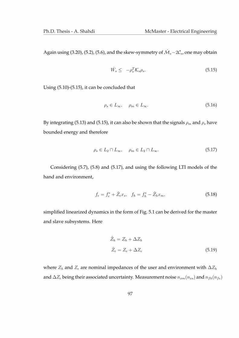
Ph.D. Thesis - A. Shahdi McMaster - Electrical Engineering
Again using (3.20), (5.2), (5.6), and the skew-symmetry of Ms−2Cs, one may obtain
Ws ≤ −ρTsKsρs. (5.15)
Using (5.10)-(5.15), it can be concluded that
ρs ∈ L∞, ρm ∈ L∞. (5.16)
By integrating (5.13) and (5.15), it can also be shown that the signals ρm and ρs have
bounded energy and therefore
ρs ∈ L2 ∩ L∞, ρm ∈ L2 ∩ L∞. (5.17)
Considering (5.7), (5.8) and (5.17), and using the following LTI models of the
hand and environment,
fe = f ∗e + Zexs, fh = f ∗h − Zhxm, (5.18)
simplified linearized dynamics in the form of Fig. 5.1 can be derived for the master
and slave subsystems. Here
Zh = Zh + ∆Zh
Ze = Ze + ∆Ze (5.19)
where Zh and Ze are nominal impedances of the user and environment with ∆Zh
and ∆Ze being their associated uncertainty. Measurement noise nxm(nxs) and nfh(nfe)
97
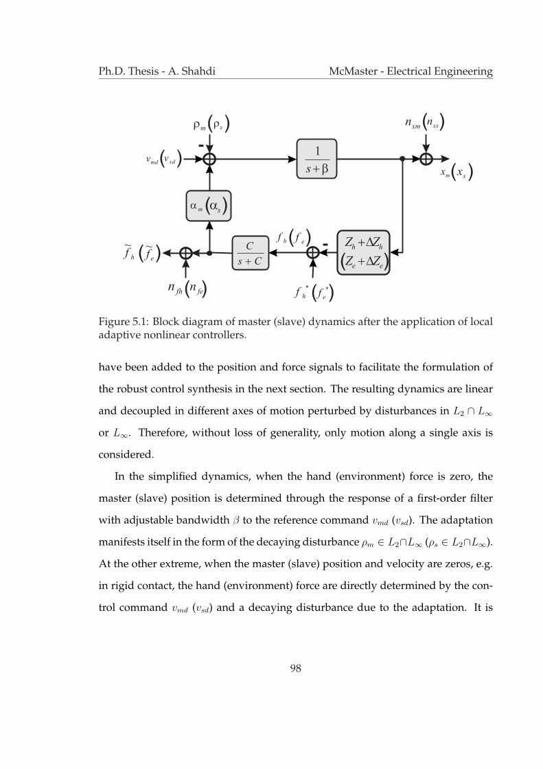
Ph.D. Thesis - A. Shahdi McMaster - Electrical Engineering
Figure 5.1: Block diagram of master (slave) dynamics after the application of localadaptive nonlinear controllers.
have been added to the position and force signals to facilitate the formulation of
the robust control synthesis in the next section. The resulting dynamics are linear
and decoupled in different axes of motion perturbed by disturbances in L2 ∩ L∞
or L∞. Therefore, without loss of generality, only motion along a single axis is
considered.
In the simplified dynamics, when the hand (environment) force is zero, the
master (slave) position is determined through the response of a first-order filter
with adjustable bandwidth β to the reference command vmd (vsd). The adaptation
manifests itself in the form of the decaying disturbance ρm ∈ L2∩L∞ (ρs ∈ L2∩L∞).
At the other extreme, when the master (slave) position and velocity are zeros, e.g.
in rigid contact, the hand (environment) force are directly determined by the con-
trol command vmd (vsd) and a decaying disturbance due to the adaptation. It is
98

Ph.D. Thesis - A. Shahdi McMaster - Electrical Engineering
clear that the application of local adaptive controllers greatly simplifies the mas-
ter/slave dynamics. This is achieved by removing the nonlinearities and elimi-
nating the system dependency on master/slave parameters. It should be noted,
however, that these linearized dynamics are still subject to uncertainty in the form
of the unknown perturbations to the operator and environment dynamics ∆Zh and
∆Ze.
A key point in the proposed two-step teleoperation approach is the decoupling
of the local master and slave adaptive controls from an outer-loop time-delay co-
ordinating controller introduced in the next section. The adaptation errors, shown
to be bounded and having finite energy in (5.17), can be modeled as bounded dis-
turbances in the robust control synthesis framework. The speed at which the local
tracking errors decay could impact the overall fidelity of the teleoperation system
in transition phases, but would not cause instability, at least from a theoretical
point of view. While selecting large feedback and adaptation gains can accelerate
the convergence of these tracking errors and reduce their effect on user perception,
unmodeled dynamics such as drive flexibility, actuator dynamics, and nonlinear
friction effects, as well as measurement noise can limit the gain values in practice.
5.3 Teleoperation Control Formulation
The coordination between master and slave robots must be achieved through the
new control signals vmd and vsd in Fig. 5.1. As stated in Chapter 3, the teleopera-
tion control objectives can be expressed in terms of delay-free position and force
tracking between the master and slave robots. Satisfying the transparency objec-
tives in (3.21) and (3.22) would provide the operator with a seamless access to the
99
Ph.D. Thesis - A. Shahdi McMaster - Electrical Engineering
task environment. However in practice, robust stability constraints arising from
the time delay and dynamic uncertainty prevent achieving ideal transparency. In-
stead, a compromise solution must be sought to balance the stability and perfor-
mance requirements. To this end, a robust time-delay teleoperation control syn-
thesis problem is formulated in this section.
A block diagram of the linearized teleoperation controllers with correspond-
ing input, output, disturbance and measurement signals is shown in Fig. 5.2. The
design objectives can be specified as reducing the filtered position and force track-
ing errors xm − xs and fh − fe in response to the two filtered exogenous forces f ∗h
and f ∗e which are the cause of motion. The addition of the filtered noise signals
nxm, nxs, nfh, and nfe, and the filtered control signals vmd and vsd at the inputs and
outputs, respectively, regularizes the design problem in order to attain a feasible
solution. The adaptive control error signals ρm and ρs, as demonstrated in (5.17),
belong to L2 ∩ L∞ space. These errors can be integrated into the robust control
formulation through the introduction of the filtered disturbance signals ρm and ρs.
The frequency-dependent gains Wjs on the signals are used to emphasize their rel-
ative importance at various frequencies and must be carefully selected to balance
the design objectives such as position and force tracking as well as robust stability.
They are also employed to characterize the frequency content of the noise and dis-
turbance signals as well as the cost associated with the control effort as a function
of frequency.
Unlike the local adaptive controllers, the teleoperation coordinating controller
is centralized and should be placed either at the master or at the slave site. In
this thesis, the controller is assumed to be at the master site with forward and
100

Ph.D. Thesis - A. Shahdi McMaster - Electrical Engineering
Figure 5.2: Linearized teleoperation control system.
101
Ph.D. Thesis - A. Shahdi McMaster - Electrical Engineering
return communication delays of τ1 and τ2 seconds, respectively. This is reflected in
Fig. 5.2 where the slave control and measurement signals are delayed by τ1 and τ2.
The teleoperation control system in Fig. 5.2 can be redrawn in the general form of
a MIMO system with multiple delays in I/O channels as shown in Fig. 5.3(a). In
this figure
u(t) =
[vmd vsd
]T
(5.20)
y(t) =
[xm fh xs fe
]T
(5.21)
w1(t) =
[fzh(t) fze(t)
]T
(5.22)
w2(t) =
[f ∗h f ∗e ρm ρs nxm nfh
nxs nfe
]T
(5.23)
z1(t) =
[vm(t) vs(t)
]T
(5.24)
z2(t) =
[xm − xs fh − fe vmd vsd
]T
(5.25)
where u(t), y(t), w(t) and z(t) are the control action, measurement, disturbance,
and output signals, respectively. Also, yc and uc are the input and the output of
the controller block. The delays in control and measurement are represented by
diagonal matrices Λu and Λy with appropriate dimensions. The diagonal entries
of these matrices are either 1 or e−sτ , depending on whether delay exists in the
102

Ph.D. Thesis - A. Shahdi McMaster - Electrical Engineering
corresponding input (output) channel or not, i.e.
Λu(s) =
e−hu,qsImq
. . .
e−hu,1sIm1
Im0
(5.26)
and
Λy(s) =
Ip0
e−hy,1sIp1
. . .
e−hy,rsIpr
(5.27)
where diagonal entries are sorted in descending (ascending) order of the delay in
input (output) channels, respectively. Note that a simple permutation of input and
output channels can transform the system into this form, if needed.
The uncertainty in the hand and environment impedances is modeled as in (5.19).
If the nominal impedances Zh and Ze are chosen based on the minimum expected
mass, damping, and stiffness parameters of the operator and environment, ∆Zh/s
and ∆Ze/s would become passive. However in this case, due to the unbounded
‖ · ‖∞ of the uncertainty blocks ∆Zh/s and ∆Ze/s, robust control methods such as
H∞ and µ-synthesis cannot be utilized directly. To resolve this issue, as proposed
in [30], the following wave variables [73] are introduced
ah = fzh + ∆Z0hvm , bh = fzh −∆Z0
hvm (5.28)
103

Ph.D. Thesis - A. Shahdi McMaster - Electrical Engineering
where ah and bh are the output and input wave variables, respectively, and ∆Z0h is
an arbitrary resistive impedance. It can be shown that
bh =[(∆Zh −∆Z0
h)(∆Zh + ∆Z0h)−1
]ah = Shah (5.29)
where Sh is the scattering operator. For passive operator dynamics, ∆Zh/s is posi-
tive real [47], i.e.1
jω[Zh(jω)− Z∗
h(jω)] ≥ 0 (5.30)
and Sh is stable and bounded real, i.e.
‖ Sh ‖∞= supω σ[Sh(jω)] ≤ 1 (5.31)
where σ[.] is the maximum singular value. The environment wave variables ae,
be, and the corresponding scattering operator Se can be similarly defined based
on fze and vs signals. The new uncertainties elements Sh and Se can be easily
incorporated into the H∞ design framework since they have bounded ‖ · ‖∞.
The application of the wave variable transformation results in a new open-loop
plant dynamics P (s), whose elements can be expressed in terms of those of P (s).
Let the first and second inputs to P (s) be w1(t) and[w2(t) u(t)
]T
, respectively,
and the first and second outputs of P (s) be z1(t) and[z2(t) y(t)
]T
, respectively. A
state-space realization of P (s) in Fig. 5.3(a) can be written as
P (s) =
A B1 B2
C1 0 D1
C2 0 D2
. (5.32)
104
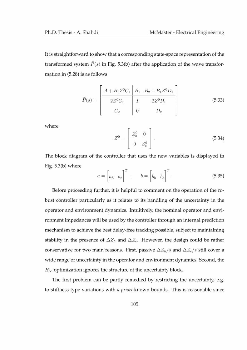
Ph.D. Thesis - A. Shahdi McMaster - Electrical Engineering
It is straightforward to show that a corresponding state-space representation of the
transformed system P (s) in Fig. 5.3(b) after the application of the wave transfor-
mation in (5.28) is as follows
P (s) =
A + B1Z0C1 B1 B2 + B1Z
0D1
2Z0C1 I 2Z0D1
C2 0 D2
(5.33)
where
Z0 =
Z0h 0
0 Z0e
. (5.34)
The block diagram of the controller that uses the new variables is displayed in
Fig. 5.3(b) where
a =
[ah ae
]T
, b =
[bh be
]T
. (5.35)
Before proceeding further, it is helpful to comment on the operation of the ro-
bust controller particularly as it relates to its handling of the uncertainty in the
operator and environment dynamics. Intuitively, the nominal operator and envi-
ronment impedances will be used by the controller through an internal prediction
mechanism to achieve the best delay-free tracking possible, subject to maintaining
stability in the presence of ∆Zh and ∆Ze. However, the design could be rather
conservative for two main reasons. First, passive ∆Zh/s and ∆Ze/s still cover a
wide range of uncertainty in the operator and environment dynamics. Second, the
H∞ optimization ignores the structure of the uncertainty block.
The first problem can be partly remedied by restricting the uncertainty, e.g.
to stiffness-type variations with a priori known bounds. This is reasonable since
105

Ph.D. Thesis - A. Shahdi McMaster - Electrical Engineering
Figure 5.3: A MIMO system with multiple I/O delays: (a) original; (b) after apply-ing the wave transformations.
the stiffness, particularly that of the environment, varies significantly in different
phases of teleoperation. In this context, the hand and environment impedances are
assumed to be in the form of
Zh,e = Kh,e + ∆Kh,e , |∆Kh,e| < Kmh,me (5.36)
where subscripts h and e refer to hand and environment, respectively. This as-
sumption will eliminate the need for the wave variable transformations and will
yield a less conservative design. Moreover, the centralized robust controller is lo-
cated at master site and the master measurement and control signals are delay free.
Thus, it can be argued that the sensitivity to the operator parameters is less than
that to the environment parameters. Therefore, the control design can be further
simplified by neglecting the variations in the operator stiffness, although such an
106

Ph.D. Thesis - A. Shahdi McMaster - Electrical Engineering
assumption may not always be applicable [128]. The second problem can poten-
tially be solved by the application of the µ-synthesis and the structured singular
value for incorporating the structure of the uncertainty into the control synthesis.
This will reduce some of the conservatism inherent in the H∞-based approach due
to ignoring the form and type of the perturbation.
5.4 H∞ Control of MIMO Systems with I/O time delay
First a couple of notations that will be used throughout the rest of this chapter are
introduced. In Fig. 5.4(a), a generic feedback control system is displayed. For this
system, the lower fractional transformation, i.e. the mapping from w to z when the
lower loop is closed by
u = Ky (5.37)
is denoted by Fl(P, K). Also, the time-delay H∞ control method mainly relies on
the so called scattering representation of systems as shown in Fig. 5.4(b). Here
Q = Cr(G, K) (5.38)
denotes the unique closed-loop mapping from η to ξ where
ξ
η
= G
u
y
(5.39)
107

Ph.D. Thesis - A. Shahdi McMaster - Electrical Engineering
Figure 5.4: (a) Lower fractional transformation (LFT); (b) Scattering representation.
and when the loop is closed by u = Ky. In the case of η and y being of the same
dimension, one may write
Cr(G, K) = (G11K + G12)(G21K + G22)−1. (5.40)
The objective of the design is to find a stabilizing controller KΛ in Fig. 5.3 that
would minimize the L∞ norm of the closed-loop transfer function, i.e.
minimize ‖Fl(P, ΛuKΛΛy)‖∞ (5.41)
from the input
w(t) =
[w1(t) w2(t)
]T
(5.42)
to the output
z(t) =
[z1(t) z2(t)
]T
(5.43)
in Fig. 5.3(a), or from the input
w(t) =
[b(t) w2(t)
]T
(5.44)
108
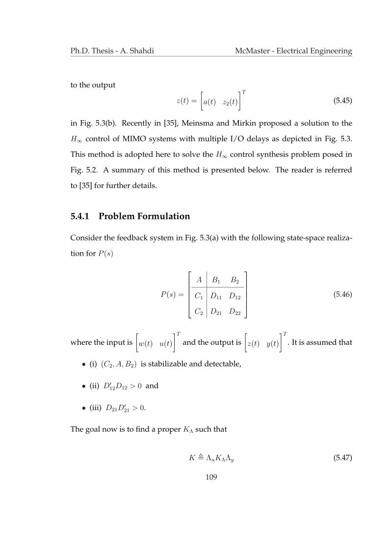
Ph.D. Thesis - A. Shahdi McMaster - Electrical Engineering
to the output
z(t) =
[a(t) z2(t)
]T
(5.45)
in Fig. 5.3(b). Recently in [35], Meinsma and Mirkin proposed a solution to the
H∞ control of MIMO systems with multiple I/O delays as depicted in Fig. 5.3.
This method is adopted here to solve the H∞ control synthesis problem posed in
Fig. 5.2. A summary of this method is presented below. The reader is referred
to [35] for further details.
5.4.1 Problem Formulation
Consider the feedback system in Fig. 5.3(a) with the following state-space realiza-
tion for P (s)
P (s) =
A B1 B2
C1 D11 D12
C2 D21 D22
(5.46)
where the input is[w(t) u(t)
]T
and the output is[z(t) y(t)
]T
. It is assumed that
• (i) (C2, A,B2) is stabilizable and detectable,
• (ii) D′12D12 > 0 and
• (iii) D21D′21 > 0.
The goal now is to find a proper KΛ such that
K , ΛuKΛΛy (5.47)
109

Ph.D. Thesis - A. Shahdi McMaster - Electrical Engineering
internally stabilizes the system and
‖Fl(P, ΛuKΛΛy)‖∞ < γ (5.48)
for a given γ > 0. It is evident that KΛ cannot be calculated simply by inverting
the mapping in (5.47) since this would result in a non-causal controller KΛ.
5.4.2 Equivalent One-block Problem
Time delay imposes additional constraints on the controller KΛ in Fig. 5.3, and
therefore, the problem has a solution only if does the delay-free problem. The
original four-block delay problem can be reduced to an equivalent one-block delay
problem using the solution to the delay-free problem [35, 129]. The resulting one-
block problem is in the form of Fig. 5.5, where G(s) is a bistable transfer matrix
with an identity feedthrough term. The solution to the delay-free H∞ problem as
well as the definition of the transfer matrix G(s) are given in Appendix D. The joint
input-output delay operator is defined as
Λ =
Λu
Λ−1y
(5.49)
where Λu and Λy are defined in (5.26) and (5.27), respectively. The noncausal el-
ements in Λ can be eliminated by multiplying it with the scalar operator e−hy,rs,
110

Ph.D. Thesis - A. Shahdi McMaster - Electrical Engineering
Figure 5.5: Equivalent one-block problem
without affecting the (η, ζ) mapping. Therefore, Λ can be written as
Λ ,
e−hq+rsInq+r
. . .
e−h1sIn1
In0
(5.50)
where 0 < h1 < · · · < hq+r and hq+r = hu,q + hy,r.
The solution to the one-block problem is a controller K which yields
‖Cr(GΛ, K)‖∞ < 1. (5.51)
The original four-block problem solution, KΛ, can be obtained from K using [35]
KΛ = Cr(D−1Λ , K) (5.52)
where DΛ is bistable, causally invertible and is defined as
DΛ , Λ−1D∞Λ. (5.53)
111
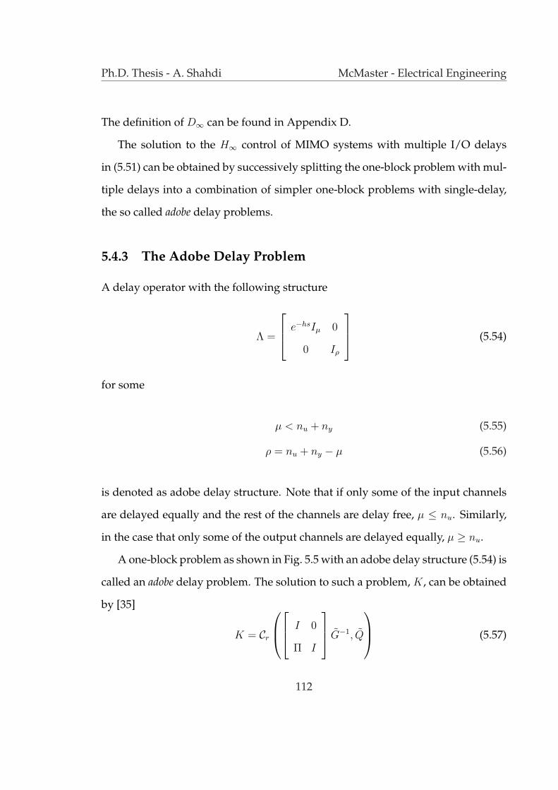
Ph.D. Thesis - A. Shahdi McMaster - Electrical Engineering
The definition of D∞ can be found in Appendix D.
The solution to the H∞ control of MIMO systems with multiple I/O delays
in (5.51) can be obtained by successively splitting the one-block problem with mul-
tiple delays into a combination of simpler one-block problems with single-delay,
the so called adobe delay problems.
5.4.3 The Adobe Delay Problem
A delay operator with the following structure
Λ =
e−hsIµ 0
0 Iρ
(5.54)
for some
µ < nu + ny (5.55)
ρ = nu + ny − µ (5.56)
is denoted as adobe delay structure. Note that if only some of the input channels
are delayed equally and the rest of the channels are delay free, µ ≤ nu. Similarly,
in the case that only some of the output channels are delayed equally, µ ≥ nu.
A one-block problem as shown in Fig. 5.5 with an adobe delay structure (5.54) is
called an adobe delay problem. The solution to such a problem, K, can be obtained
by [35]
K = Cr
I 0
Π I
G−1, Q
(5.57)
112

Ph.D. Thesis - A. Shahdi McMaster - Electrical Engineering
where G(s) is a bistable transfer matrix, Π(s) is an Finite-Impulse-Response (FIR)
operator, and Q is contractive, i.e.
‖Q‖∞ < 1. (5.58)
The reader is referred to Appendix E for the actual forms of Π, G, and Q. Alterna-
tively, it can be shown that
Q = Cr
G
I 0
−Π I
, K
(5.59)
is a contraction.
5.4.4 Decomposition
The multiple-delay one-block problem (G, Λ), as shown in Fig 5.5, can be decom-
posed to a series of single-delay adobe problems, the solution of which was pre-
sented in the last subsection. The delay operator Λ in (5.50) includes q + r ordered
delay blocks referred to as (q + r)-delay operator. It can be easily shown that [35]
Λ = Λ1Λ (5.60)
where
Λ1 ,
e−h1sIµ1 0
0 Iρ1
, ρ1 = n0 (5.61)
113

Ph.D. Thesis - A. Shahdi McMaster - Electrical Engineering
is a delay operator of the adobe form and Λ is a (q + r − 1)-delay operator with
(n0 + n1) delay-free channels. Using (5.60), one may write
Cr(GΛ, K) = Cr
(GΛ1, Cr(Λ, K)
). (5.62)
Therefore, the original multiple-delay problem (G, Λ) has solution only if the adobe
delay problem (G, Λ1) has one, i.e.
Q , Cr
G
I 0
−Π I
, Cr(Λ, K)
(5.63)
is a contraction. By absorbing the term
I 0
−Π I
into the controller one can write
Q = Cr(GΛ, K) (5.64)
where
K = Cr
Λ−1
I 0
−Π I
Λ, K
. (5.65)
Due to the fact that
I 0
−Π I
has a lower triangular structure and the delays in
Λ are ordered descendantly, the term Λ−1
I 0
−Π I
Λ is bistable with an identity
feedthrough term. Therefore, K is proper if and only if K is proper. Hence, a
114

Ph.D. Thesis - A. Shahdi McMaster - Electrical Engineering
proper choice of K can make Q contractive if and only if there is a K such that
‖Cr(GΛ, K)‖∞ < 1. (5.66)
In other words, the original multiple-delay problem is equivalent to a combination
of a single-delay adobe problem and a multiple-delay problem with an order less
than that of the original problem given in (5.66). This iterative procedure is contin-
ued until a one-block problem with (0)-delay operator is resulted, the solution of
which can be obtained by inverting its transfer function.
5.5 Design Example
The proposed mixed adaptive/roboust controller is applied to a two-axis teleoper-
ation system involving two kinematically and dynamically similar two-degree-of-
freedom robots. Due to the decoupling of dynamics through the first-stage adap-
tive controllers, only the design and analysis of the robust controller along a single
axis is discussed here. The mechanical design of the robots, which will be intro-
duced in the next section, is such that linear mass-damper-spring models with
unknown parameters can sufficiently described their dynamics. Therefore, such
models are used in the local adaptive controllers.
The system and controller parameters are given in Table 5.1. The system param-
eters reflect those of the experimental setup. It should be noted that no knowledge
of the master and slave robot parameters is required by the controller because of
the use of the local adaptive controllers. Typical values have been selected for the
115
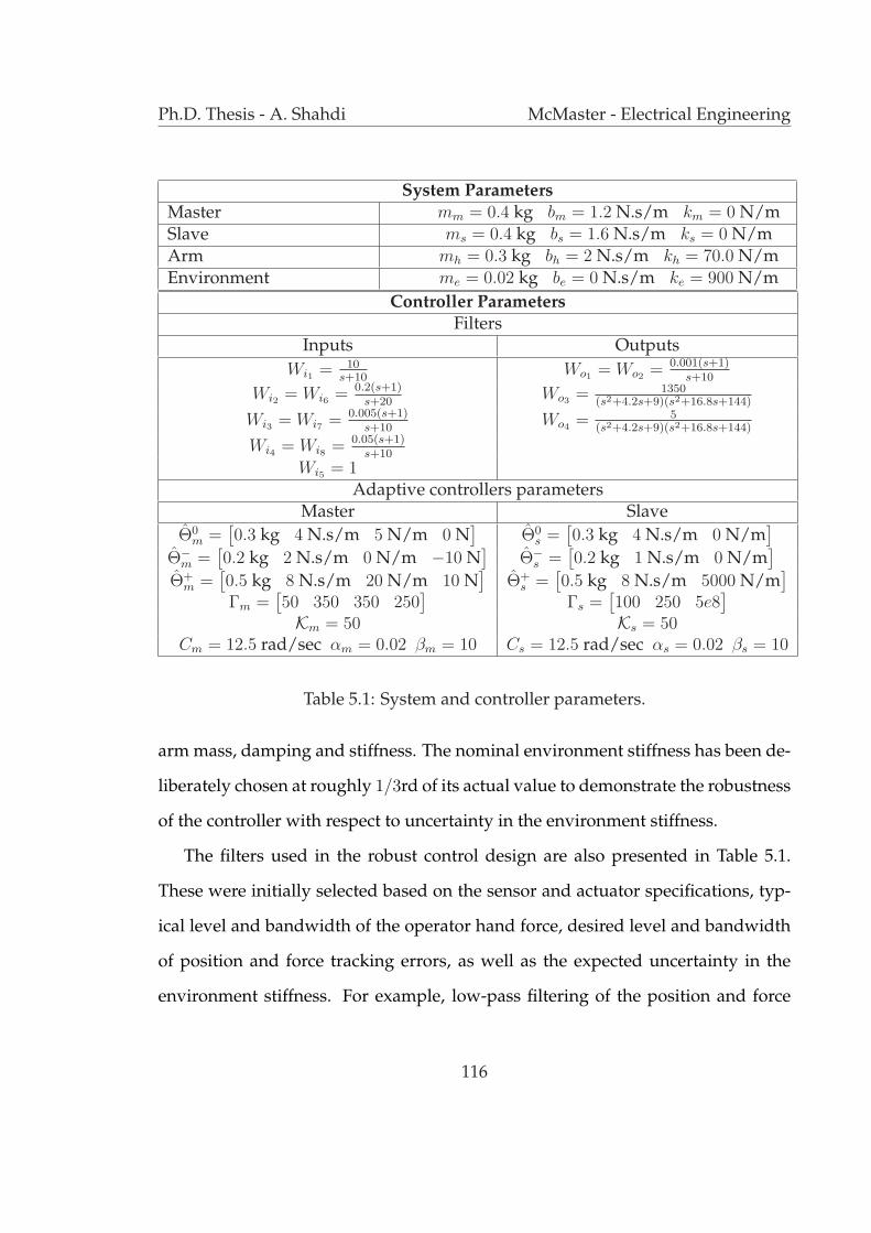
Ph.D. Thesis - A. Shahdi McMaster - Electrical Engineering
System ParametersMaster mm = 0.4 kg bm = 1.2 N.s/m km = 0 N/mSlave ms = 0.4 kg bs = 1.6 N.s/m ks = 0 N/mArm mh = 0.3 kg bh = 2 N.s/m kh = 70.0 N/mEnvironment me = 0.02 kg be = 0 N.s/m ke = 900 N/m
Controller ParametersFilters
Inputs OutputsWi1 = 10
s+10Wo1 = Wo2 = 0.001(s+1)
s+10
Wi2 = Wi6 = 0.2(s+1)s+20
Wo3 = 1350(s2+4.2s+9)(s2+16.8s+144)
Wi3 = Wi7 = 0.005(s+1)s+10
Wo4 = 5(s2+4.2s+9)(s2+16.8s+144)
Wi4 = Wi8 = 0.05(s+1)s+10
Wi5 = 1Adaptive controllers parameters
Master SlaveΘ0
m =[0.3 kg 4 N.s/m 5 N/m 0 N
]Θ0
s =[0.3 kg 4 N.s/m 0 N/m
]Θ−
m =[0.2 kg 2 N.s/m 0 N/m −10 N
]Θ−
s =[0.2 kg 1 N.s/m 0 N/m
]Θ+
m =[0.5 kg 8 N.s/m 20 N/m 10 N
]Θ+
s =[0.5 kg 8 N.s/m 5000 N/m
]Γm =
[50 350 350 250
]Γs =
[100 250 5e8
]Km = 50 Ks = 50
Cm = 12.5 rad/sec αm = 0.02 βm = 10 Cs = 12.5 rad/sec αs = 0.02 βs = 10
Table 5.1: System and controller parameters.
arm mass, damping and stiffness. The nominal environment stiffness has been de-
liberately chosen at roughly 1/3rd of its actual value to demonstrate the robustness
of the controller with respect to uncertainty in the environment stiffness.
The filters used in the robust control design are also presented in Table 5.1.
These were initially selected based on the sensor and actuator specifications, typ-
ical level and bandwidth of the operator hand force, desired level and bandwidth
of position and force tracking errors, as well as the expected uncertainty in the
environment stiffness. For example, low-pass filtering of the position and force
116
Ph.D. Thesis - A. Shahdi McMaster - Electrical Engineering
tracking errors emphasizes on transparency at low frequency whereas high pass-
filtering of the noise inputs reflects the fact that the noise power is mostly concen-
trated at high frequency. Moreover, high-pass filtering of the control commands
at the output penalizes undesirable high frequency control activities. The ini-
tial filters were further adjusted based on simulation and experimental results to
achieve a balance between the robust stability and performance requirements. For
instance, increasing the gains and bandwidth of the position and force tracking
error filters, while enhancing transparency, can reduce the stability margin with
respect to variations in the environment stiffness. This could also result in ex-
cessively tight control loops with high-frequency modes that would require high
sampling rates for discrete-time implementation.
The original four-block delay problem of the teleoperation control system is
shown in Fig. 5.2. The equivalent one-block delay problem can be obtained using
the delay-free solution and following the steps outlined in the previous section and
Appendix D. In this case, the input and output delay operators are
Λu =
e−sτ1
1
(5.67)
and
Λy =
I2
e−sτ2I2
. (5.68)
Using (5.49) and after eliminating the noncausal elements, the joint input/output
117
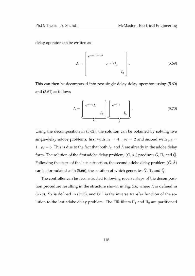
Ph.D. Thesis - A. Shahdi McMaster - Electrical Engineering
delay operator can be written as
Λ =
e−s(τ1+τ2)
e−sτ2I3
I2
. (5.69)
This can then be decomposed into two single-delay delay operators using (5.60)
and (5.61) as follows
Λ =
e−sτ2I4
I2
︸ ︷︷ ︸Λ1
e−sτ1
I5
︸ ︷︷ ︸Λ
. (5.70)
Using the decomposition in (5.62), the solution can be obtained by solving two
single-delay adobe problems, first with µ1 = 4 , ρ1 = 2 and second with µ2 =
1 , ρ2 = 5. This is due to the fact that both Λ1 and Λ are already in the adobe delay
form. The solution of the first adobe delay problem, (G, Λ1) produces G, Π1 and Q.
Following the steps of the last subsection, the second adobe delay problem (G, Λ)
can be formulated as in (5.66), the solution of which generates G, Π2 and Q.
The controller can be reconstructed following reverse steps of the decomposi-
tion procedure resulting in the structure shown in Fig. 5.6, where Λ is defined in
(5.70), DΛ is defined in (5.53), and G−1 is the inverse transfer function of the so-
lution to the last adobe delay problem. The FIR filters Π1 and Π2 are partitioned
118
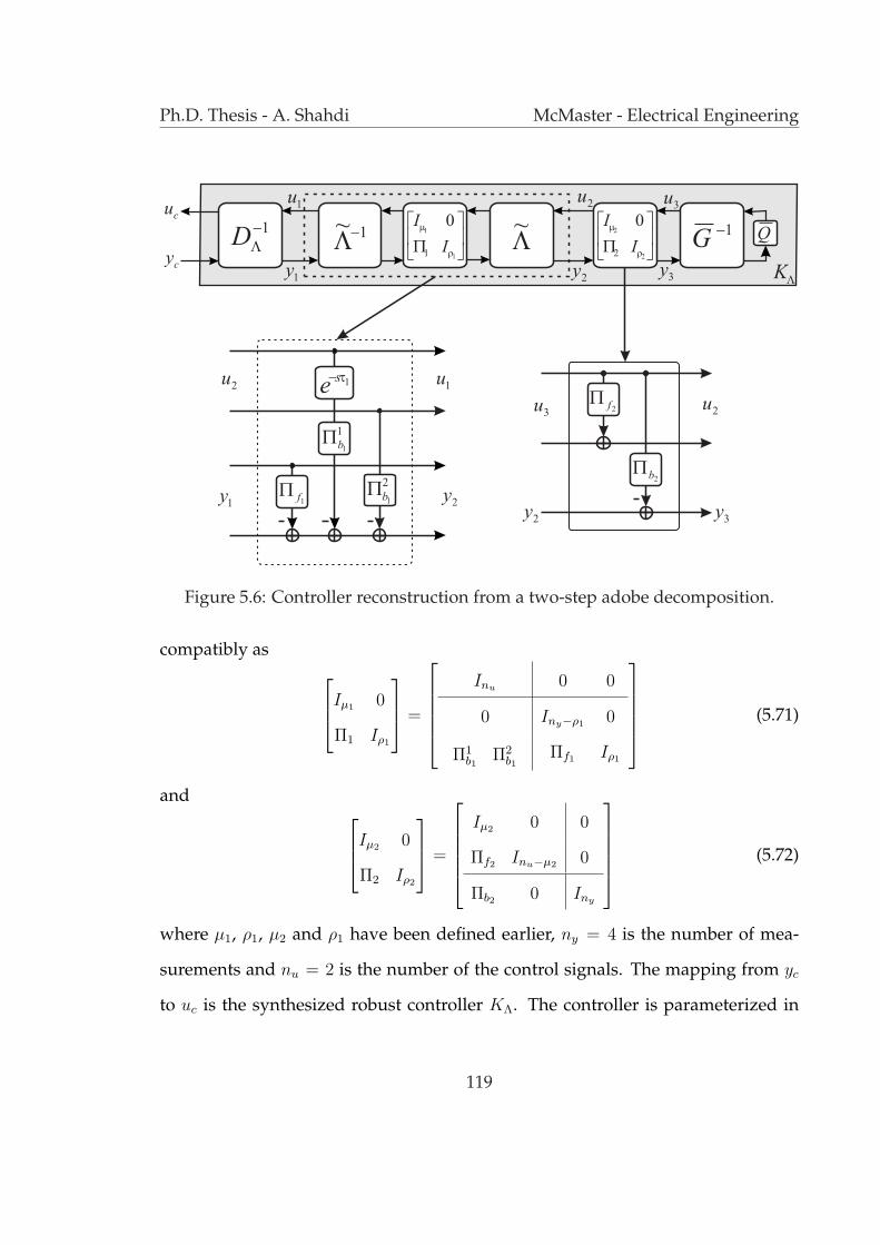
Ph.D. Thesis - A. Shahdi McMaster - Electrical Engineering
Figure 5.6: Controller reconstruction from a two-step adobe decomposition.
compatibly as
Iµ1 0
Π1 Iρ1
=
Inu 0 0
0 Iny−ρ1 0
Π1b1
Π2b1
Πf1 Iρ1
(5.71)
and
Iµ2 0
Π2 Iρ2
=
Iµ2 0 0
Πf2 Inu−µ2 0
Πb2 0 Iny
(5.72)
where µ1, ρ1, µ2 and ρ1 have been defined earlier, ny = 4 is the number of mea-
surements and nu = 2 is the number of the control signals. The mapping from yc
to uc is the synthesized robust controller KΛ. The controller is parameterized in
119

Ph.D. Thesis - A. Shahdi McMaster - Electrical Engineering
terms of a contractive mapping Q which is chosen to be zero. It is worth noticing
that the local adaptive controllers require u =
[vmd vsd
]T
in their implementa-
tion. This can be calculated using the linearity of the robust controller and based
on y. The definition of y in Fig. 5.3 reveals that only velocity and force signals are
required for the implementation. Alternatively, given that there is no feedthrough
term from the measurement to control in the robust controller, the derivatives can
also be computed based on yc and a revised dynamics derived from the controller.
Throughout the rest of the chapter, the communication delay in both directions
are assumed equal, i.e. τ1 = τ2 = τ msec. Also, the delay values correspond to
a round-trip delay unless otherwise stated. The closed-loop frequency responses
from the user exogenous force input f ∗h to the system outputs xm, xs, fh, and fe
for three different delays, i.e. 100 msec, 200 msec and 300 msec, are displayed in
Figs. 5.7-5.12. Two cases have been considered for each delay, first when the actual
environment stiffness matches that used in the design, i.e. ke = ke = 900 N/m
(Figs. 5.7, 5.9, 5.11) and then when there is a mismatch between these values, i.e.
ke = 2000 N/m (actual) and ke = 900 N/m (design)(Figs. 5.8, 5.10, 5.12). From
these figures, it can be seen that the transparency objectives have been met for
frequencies up to 4.0 ∼ 6.0 Hz for the matched environment stiffness. This is above
the average hand voluntary movement frequency range of 0 ∼ 2 Hz reported in
the literature [130]. Although the system transparency would degrade to some
extent in the mismatch case and by increase in communication delay, the results
are still satisfactory and demonstrate robust performance of the controller.
The robust controller has been designed for a nominal environment stiffness of
ke = 900 N/m. The stability margins of the controller with respect to variations
120
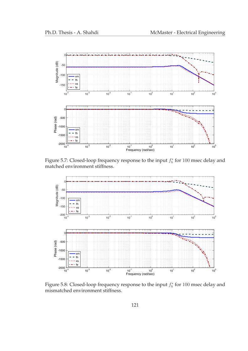
Ph.D. Thesis - A. Shahdi McMaster - Electrical Engineering
Figure 5.7: Closed-loop frequency response to the input f ∗h for 100 msec delay andmatched environment stiffness.
Figure 5.8: Closed-loop frequency response to the input f ∗h for 100 msec delay andmismatched environment stiffness.
121

Ph.D. Thesis - A. Shahdi McMaster - Electrical Engineering
Figure 5.9: Closed-loop frequency response to the input f ∗h for 200 msec delay andmatched environment stiffness.
Figure 5.10: Closed-loop frequency response to the input f ∗h for 200 msec delay andmismatched environment stiffness.
122

Ph.D. Thesis - A. Shahdi McMaster - Electrical Engineering
Figure 5.11: Closed-loop frequency response to the input f ∗h for 300 msec delay andmatched environment stiffness.
Figure 5.12: Closed-loop frequency response to the input f ∗h for 300 msec delay andmismatched environment stiffness.
123

Ph.D. Thesis - A. Shahdi McMaster - Electrical Engineering
Figure 5.13: The closed-loop system subject to the environment stiffness uncer-tainty, δke.
in the environment stiffness can be examined with the aid of the Nyquist analysis.
A model of closed-loop system subject to the stiffness uncertainty is displayed in
Fig. 5.13. The characteristic equation of the perturbed system is given by
1− δkeR(s) = 0. (5.73)
The Nyquist plots of R(s) for delays of 100, 200, and 300 msec are depicted in
Fig. 5.14-5.16. Given that the unperturbed system is stable, it can be concluded
that the system remains stable as long as the Nyquist plot of R(s) does not en-
circle 1/δke. Therefore, the system stability is guaranteed for perturbations in the
124
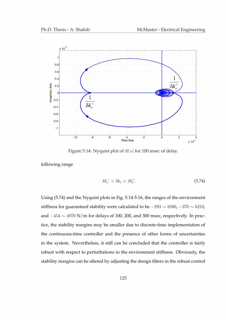
Ph.D. Thesis - A. Shahdi McMaster - Electrical Engineering
Figure 5.14: Nyquist plot of R(s) for 100 msec of delay.
following range
δk−e < δke < δk+e . (5.74)
Using (5.74) and the Nyquist plots in Fig. 5.14-5.16, the ranges of the environment
stiffness for guaranteed stability were calculated to be −293 ∼ 8500, −370 ∼ 6210,
and −454 ∼ 4970 N/m for delays of 100, 200, and 300 msec, respectively. In prac-
tice, the stability margins may be smaller due to discrete-time implementation of
the continuous-time controller and the presence of other forms of uncertainties
in the system. Nevertheless, it still can be concluded that the controller is fairly
robust with respect to perturbations in the environment stiffness. Obviously, the
stability margins can be altered by adjusting the design filters in the robust control
125

Ph.D. Thesis - A. Shahdi McMaster - Electrical Engineering
Figure 5.15: Nyquist plot of R(s) for 200 msec of delay.
Figure 5.16: Nyquist plot of R(s) for 300 msec of delay.
126

Ph.D. Thesis - A. Shahdi McMaster - Electrical Engineering
formulation to achieve a new trade-off between transparency and robust stability.
5.6 Experimental Results
The same experimental setup, as shown in Fig. 4.9, has been utilized here to verify
the effectiveness of the proposed control method. A block diagram of the pro-
posed two-stage controller is shown in Fig. 5.17. The local adaptive controllers
are implemented using the procedure outlined in Section 2 and based on the pa-
rameters given in Table 5.1. The parameters and filters used in the design of the
outer-loop robust controller are also given in this table. The implementation of the
robust controller involves two FIR filters Π1 and Π2 in Fig. 5.6 with the form given
in (E.82)-(E.84) in Appendix E. These filters require buffering and multiplications
of signals at a number of samples proportional to the amount of the time delay, i.e.
the length of their impulse response, and the control update rate. In the particular
example of this chapter, the length of the FIR filters are 100, 200, and 300 samples
for round-trip delays of 100, 200, and 300 msec, respectively. The other component
of the controller is the plant G(s)−1 in Fig. 5.17 which has 23 states, six(6) inputs,
and six(6) outputs in the design example.
In the experiments, the operator manipulates the slave robot in free motion
and in contact with an environment with an stiffness of 2000-3000 N/m. How-
ever, as noted in Table 5.1, the nominal environment stiffness was chosen to be
Ke = 900 N/m in the design. In general, interaction with stiffer environments
would require a higher design stiffness compromising the performance in interac-
tion with softer environments and in free motion. Alternatively the robust stability
margin with respect to the environment stiffness can be enlarged at the expense of
127
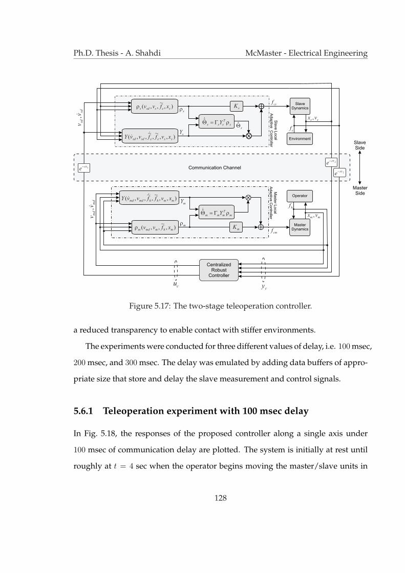
Ph.D. Thesis - A. Shahdi McMaster - Electrical Engineering
Figure 5.17: The two-stage teleoperation controller.
a reduced transparency to enable contact with stiffer environments.
The experiments were conducted for three different values of delay, i.e. 100 msec,
200 msec, and 300 msec. The delay was emulated by adding data buffers of appro-
priate size that store and delay the slave measurement and control signals.
5.6.1 Teleoperation experiment with 100 msec delay
In Fig. 5.18, the responses of the proposed controller along a single axis under
100 msec of communication delay are plotted. The system is initially at rest until
roughly at t = 4 sec when the operator begins moving the master/slave units in
128
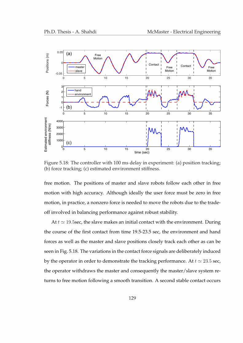
Ph.D. Thesis - A. Shahdi McMaster - Electrical Engineering
Figure 5.18: The controller with 100 ms delay in experiment: (a) position tracking;(b) force tracking; (c) estimated environment stiffness.
free motion. The positions of master and slave robots follow each other in free
motion with high accuracy. Although ideally the user force must be zero in free
motion, in practice, a nonzero force is needed to move the robots due to the trade-
off involved in balancing performance against robust stability.
At t ' 19.5sec, the slave makes an initial contact with the environment. During
the course of the first contact from time 19.5-23.5 sec, the environment and hand
forces as well as the master and slave positions closely track each other as can be
seen in Fig. 5.18. The variations in the contact force signals are deliberately induced
by the operator in order to demonstrate the tracking performance. At t ' 23.5 sec,
the operator withdraws the master and consequently the master/slave system re-
turns to free motion following a smooth transition. A second stable contact occurs
129

Ph.D. Thesis - A. Shahdi McMaster - Electrical Engineering
Figure 5.19: The controller with 200 ms delay in experiment: (a) position tracking;(b) force tracking; (c) estimated environment stiffness.
at t ' 27sec followed by another period of free motion. The estimated environment
stiffness is plotted in Fig. 5.18(c) from which it is evident that the local adaptive
controller rapidly copes with the variations in the environment stiffness.
5.6.2 Teleoperation experiment with 200 msec delay
Fig. 5.19 illustrates the responses of the controller for a round-trip delay of 200 msec.
As in the previous case, the experiments starts with the master/slave at rest, fol-
lowed by a free motion operation and subsequent contact and free motion phases.
The transitions from free motion to contact and vise versa are stable. The position
tracking in free motion as well as position and force tracking in contact are quite
satisfactory. The stiffness adaption is also demonstrated in Fig. 5.19(c).
130

Ph.D. Thesis - A. Shahdi McMaster - Electrical Engineering
Figure 5.20: The controller with 300 ms delay in experiment: (a) position tracking;(b) force tracking; (c) estimated environment stiffness.
5.6.3 Teleoperation experiment with 300 msec delay
In Fig. 5.20, the results of an experiment with the proposed teleoperation controller
under 300 msec of communication latency are presented. Once again, the transi-
tions are stable and despite a slight degradation in the tracking results, the perfor-
mance of the system is still satisfactory.
5.7 Conclusions
In this chapter, a two-stage adaptive/robust control was introduced to balance
the performance and stability requirements in time-delay teleoperation. Through
the use of local Lyapunov-based adaptive controllers, the dynamics of the master
131

Ph.D. Thesis - A. Shahdi McMaster - Electrical Engineering
and slave robots were linearized and rendered independent from their parameters.
Using these new dynamics, teleoperation control for achieving transparency and
robust stability was formulated as an H∞ robust control synthesis with multiple
I/O delays. The resulting problem was solved using decompositions into single-
delay adobe-type problems. The interaction between the local adaptive/nonlinear
controllers and the robust controller was accounted for in the proposed modeling
and control synthesis.
The results of performance and stability analysis as well as experiments with a
teleoperation setup demonstrated the effectiveness of the proposed adaptive/robust
controller. Compared to our earlier proposed model-based controllers, the robust
controller in this chapter is less sensitive to modeling uncertainties. Neverthe-
less, since it uses fixed structure and parameters for the entire range of operation,
its transparency may be sacrificed in favor of robust stability, particulary if large
modeling uncertainty is considered in the design stage.
132

Chapter 6
Adaptive Control of Bilateral
Time-delay Teleoperation
6.1 Introduction
The robust controller proposed in the previous chapter has less sensitivity to un-
certainties compared to the earlier decentralized and centralized model-based con-
trollers in Chapter 4 and [1, 2]. However, it utilizes a fixed controller for the entire
range of operation, forcing a compromise between transparency and robust sta-
bility. By varying its structure and/or parameters an adaptive controller can po-
tentially achieve a better transparency-stability trade-off in bilateral teleoperation.
This chapter introduces a new adaptive model-predictive controller for teleopera-
tion systems with constant and time-varying communication delay. The proposed
method uses the model and delay information and can adapt to uncertainties in
user and environment dynamics in order to achieve delay-free position tracking
and tool impedance shaping. A delay reduction formulation is developed which
133
Ph.D. Thesis - A. Shahdi McMaster - Electrical Engineering
utilizes the estimates of the system parameters to predict the system’s future state.
The future state of the system is then used to calculate the control action that would
regulate the system outputs to zero. A Lyapunov analysis is used to prove the sta-
bility of the system and to obtain parameter adaptation law.
This chapter is organized as follows. A revised state-space formulation of time-
delay teleoperation dynamics is presented in Section 6.2. In Section 6.3, the pro-
posed model reduction and state prediction techniques are introduced for constant
known delays. In Section 6.4, an output regulation control for achieving the trans-
parency objectives is discussed. The proof of stability and the derivation of the
adaptation law are given in Section 6.5. Parameter convergence and a compos-
ite adaptive variation of the controller are discussed in Section 6.6. In Section 6.7,
the proposed reduction technique is reformulated to accommodate for variable
latencies in the teleoperation communication channel. Section 6.8 presents the ex-
perimental results for both constant and variable time-delay cases. The chapter is
concluded in Section 6.9.
6.2 Revised Time-delay Teleoperation System Formu-
lation
In the proposed adaptive controller, a centralized architecture is assumed in which
the teleoperation controller may reside either at the master or slave site. Without
loss of generality, we assume the controller to be located at the master site. As
illustrated in Fig. 4.1, teleoperation control involves the transmission of force, po-
sition/velcoity and control action signals in both directions via a communication
134

Ph.D. Thesis - A. Shahdi McMaster - Electrical Engineering
channel that is subject to delay. The slave measurements will arrive at the con-
troller site with τ2 time delay, and the slave control action is delayed by τ1. Note
that in general the communication delays can be a function of time.
The combined nonlinear dynamics of master/hand and slave/environment
have previously been presented in (3.19) and (3.20), respectively. Following the
same steps as those in Section 4.2, these nonlinear dynamics can be linearized us-
ing an adaptive Lyapunov-based method. By choosing the master and slave po-
sition and velocity as state variables, the linearized dynamics can be written in
state-space form as presented in Appendix A.
In the proposed adaptive control framework, all the input and all the output
channels should include the same amount of latency. Therefore, the master mea-
surements and the master control action are padded by extra τ2 and τ1 delay, re-
spectively. Since the system dynamics have been linearized, the delay in the output
measurement channels can be relocated to the input channels resulting in a system
with d = τ1 + τ2 delay in all of the control signals, as illustrated in Fig. 6.1. The
round-trip delay, d, in general is variable and can be expressed as a function of
time, i.e.
d(t) = τ1(t) + τ2(t). (6.1)
The teleoperation transparency objectives used in the proposed method are the
same as those used in Chapter 4, i.e. position tracking and virtual tool impedance
shaping in (3.23)-(3.25). Here the states of the system are defined as combination
of the master, slave, and tool states as follows
X(t) =
[Xs(t) αpXs(t)−Xm(t) Xm(t)−Xt(t)
]T
(6.2)
135
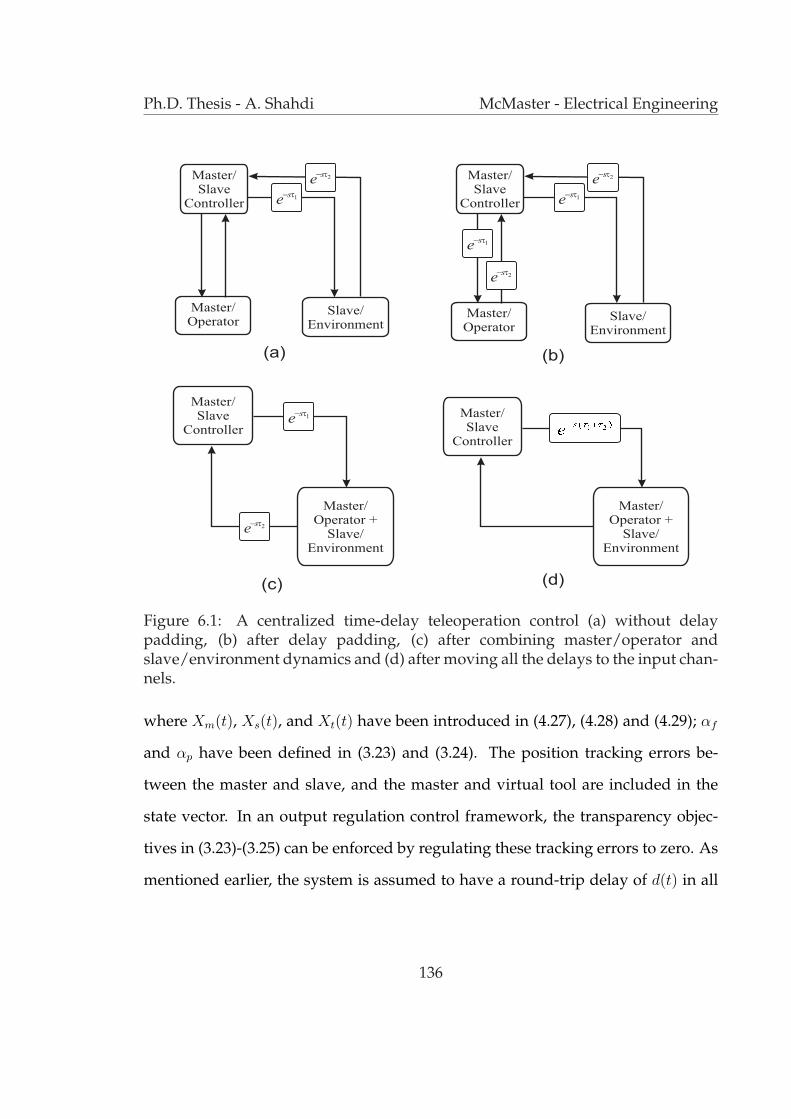
Ph.D. Thesis - A. Shahdi McMaster - Electrical Engineering
Figure 6.1: A centralized time-delay teleoperation control (a) without delaypadding, (b) after delay padding, (c) after combining master/operator andslave/environment dynamics and (d) after moving all the delays to the input chan-nels.
where Xm(t), Xs(t), and Xt(t) have been introduced in (4.27), (4.28) and (4.29); αf
and αp have been defined in (3.23) and (3.24). The position tracking errors be-
tween the master and slave, and the master and virtual tool are included in the
state vector. In an output regulation control framework, the transparency objec-
tives in (3.23)-(3.25) can be enforced by regulating these tracking errors to zero. As
mentioned earlier, the system is assumed to have a round-trip delay of d(t) in all
136
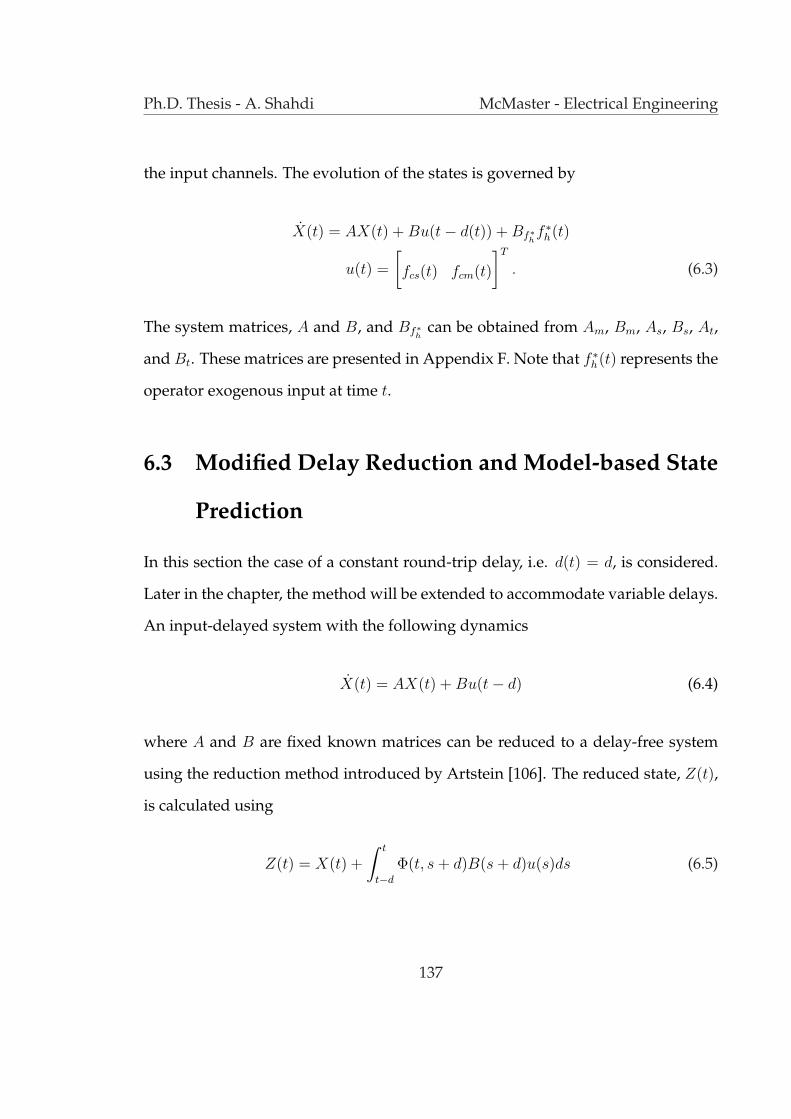
Ph.D. Thesis - A. Shahdi McMaster - Electrical Engineering
the input channels. The evolution of the states is governed by
X(t) = AX(t) + Bu(t− d(t)) + Bf∗hf ∗h(t)
u(t) =
[fcs(t) fcm(t)
]T
. (6.3)
The system matrices, A and B, and Bf∗h can be obtained from Am, Bm, As, Bs, At,
and Bt. These matrices are presented in Appendix F. Note that f ∗h(t) represents the
operator exogenous input at time t.
6.3 Modified Delay Reduction and Model-based State
Prediction
In this section the case of a constant round-trip delay, i.e. d(t) = d, is considered.
Later in the chapter, the method will be extended to accommodate variable delays.
An input-delayed system with the following dynamics
X(t) = AX(t) + Bu(t− d) (6.4)
where A and B are fixed known matrices can be reduced to a delay-free system
using the reduction method introduced by Artstein [106]. The reduced state, Z(t),
is calculated using
Z(t) = X(t) +
∫ t
t−d
Φ(t, s + d)B(s + d)u(s)ds (6.5)
137
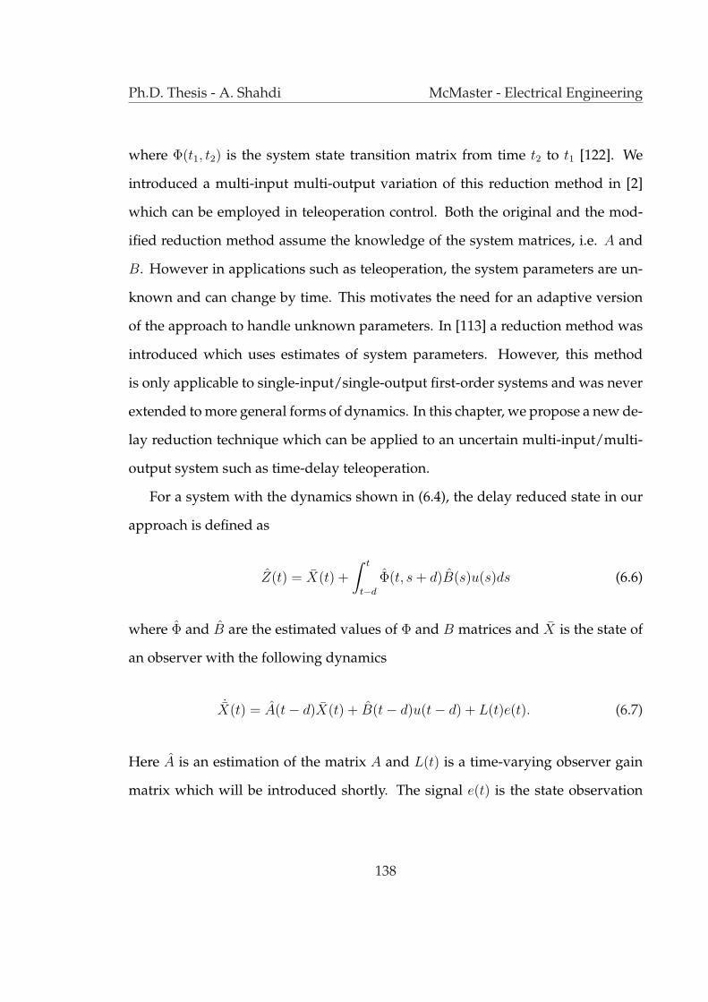
Ph.D. Thesis - A. Shahdi McMaster - Electrical Engineering
where Φ(t1, t2) is the system state transition matrix from time t2 to t1 [122]. We
introduced a multi-input multi-output variation of this reduction method in [2]
which can be employed in teleoperation control. Both the original and the mod-
ified reduction method assume the knowledge of the system matrices, i.e. A and
B. However in applications such as teleoperation, the system parameters are un-
known and can change by time. This motivates the need for an adaptive version
of the approach to handle unknown parameters. In [113] a reduction method was
introduced which uses estimates of system parameters. However, this method
is only applicable to single-input/single-output first-order systems and was never
extended to more general forms of dynamics. In this chapter, we propose a new de-
lay reduction technique which can be applied to an uncertain multi-input/multi-
output system such as time-delay teleoperation.
For a system with the dynamics shown in (6.4), the delay reduced state in our
approach is defined as
Z(t) = X(t) +
∫ t
t−d
Φ(t, s + d)B(s)u(s)ds (6.6)
where Φ and B are the estimated values of Φ and B matrices and X is the state of
an observer with the following dynamics
˙X(t) = A(t− d)X(t) + B(t− d)u(t− d) + L(t)e(t). (6.7)
Here A is an estimation of the matrix A and L(t) is a time-varying observer gain
matrix which will be introduced shortly. The signal e(t) is the state observation
138

Ph.D. Thesis - A. Shahdi McMaster - Electrical Engineering
error, i.e.
e(t) = X(t)− X(t). (6.8)
By applying the new reduction method to the teleoperation system defined in (6.3),
one can write
Z(t) = X(t) +
∫ t
t−d
Φ(t, s + d)B(s)u(s)ds +
∫ t
t−d
Φ(t, s + d) ˆBf ∗h(s)ds (6.9)
and
˙X(t) = A(t− d)X(t) + B(t− d)u(t− d) + ˆBf ∗h(t− d) + L(t)e(t) (6.10)
where ˆBf ∗h(t−d) is the estimation of Bf∗hf ∗h(t) at time t−d. Equations (6.9) and (6.10)
use the estimated values of the system parameters the calculation of which will
be discussed in the following sections. The dynamics of the reduced system can
be calculated by finding the derivative of Z(t) in (6.9) and by using the Leibniz
integral rule [131] as
˙Z(t) = ˙X(t) + Φ(t, t + d)B(t)u(t) + Φ(t, t + d) ˆBf ∗h(t)
− B(t− d)u(t− d)− ˆBf ∗h(t− d)
+
∫ t
t−d
∂
∂tΦ(t, s + d)B(s)u(s)ds +
∫ t
t−d
∂
∂tΦ(t, s + d) ˆBf ∗h(s)ds. (6.11)
139

Ph.D. Thesis - A. Shahdi McMaster - Electrical Engineering
The estimated system transition matrix, Φ(t, s), satisfies the following
∂Φ(t, s)
∂t= A(t− d)Φ(t, s) , Φ(s, s) = I (6.12)
where A is an estimation of the matrix A. Using the definition in (6.12) and Equa-
tion (6.9), the dynamics of the reduced state in (6.11) can be written as
˙Z(t) = ˙X(t) + Φ(t, t + d)B(t)u(t) + Φ(t, t + d) ˆBf ∗h(t)
− B(t− d)u(t− d)− ˆBf ∗h(t− d) + A(t− d)(Z(t)− X(t)
). (6.13)
By substituting ˙X from (6.10), one can write
˙Z(t) = A(t− d)Z(t) + Φ(t, t + d)B(t)u(t) + Φ(t, t + d) ˆBf ∗h(t) + L(t)e(t). (6.14)
The predicted state of the system in future, X(t+d), is calculated from the reduced
state, Z(t), using the following equation
X(t + d) = Φ(t + d, t)Z(t). (6.15)
The vector X(t + d) represents the predicted future state of the system which is
calculated based on the current state of the system, current information of the
model parameters and the future inputs to the system. Future inputs up to the
time t + d are available since the computed control action is buffered and applied
to the system with a delay d. Using (6.15), the derivative of the predicted state can
140

Ph.D. Thesis - A. Shahdi McMaster - Electrical Engineering
be obtained by
˙X(t + d) =
˙Φ(t + d, t)Z(t) + Φ(t + d, t)
˙Z(t). (6.16)
To find the derivative of the system transfer matrix, Φ(t + d, t) in (6.16), the follow-
ing properties are being utilized [122]
Φ(t + d, t) = Φ(t + d, τ)Φ(τ, t), (6.17)
Φ(t, τ)Φ(τ, t) = I (6.18)
where τ is an arbitrary time and I is the identity matrix of the appropriate dimen-
sion. The derivative of the equation in (6.18) is calculated as
∂Φ(t, τ)
∂tΦ(τ, t) + Φ(t, τ)
∂Φ(τ, t)
∂t= 0. (6.19)
Using the definitions in (6.12) and (6.18), Equation (6.19) can be rewritten as
A(t− d) + Φ(t, τ)∂Φ(τ, t)
∂t= 0. (6.20)
After multiplying both sides of (6.20) by Φ(τ, t) from left, one can write
∂Φ(τ, t)
∂t= −Φ(τ, t)A(t− d). (6.21)
Now taking the derivative of (6.17), one may write
˙Φ(t + d, t) =
∂Φ(t + d, τ)
∂tΦ(τ, t) + Φ(t + d, τ)
∂Φ(τ, t)
∂t. (6.22)
141

Ph.D. Thesis - A. Shahdi McMaster - Electrical Engineering
Using the definition in (6.12) and the result in (6.21), (6.22) can be rewritten as
˙Φ(t + d, t) = A(t)Φ(t + d, t)− Φ(t + d, t)A(t− d). (6.23)
The dynamics of the predicted state, X(t + d), can now be found using (6.16) and
by replacing ˙Φ(t + d, t) and ˙
Z(t) from (6.23) and (6.14) as
˙X(t + d) =
(A(t)Φ(t + d, t)− Φ(t + d, t)A(t− d)
)Z(t)
+ Φ(t + d, t)(A(t− d)Z(t) + Φ(t, t + d)B(t)u(t)
+Φ(t, t + d) ˆBf ∗h(t) + L(t)e(t))
. (6.24)
Simplifying this equation results in the following dynamics for the predicted state
˙X(t + d) = A(t)X(t + d) + B(t)u(t) + ˆBf ∗h(t) + Φ(t + d, t)L(t)e(t). (6.25)
The estimated predicted state, X(t + d), has the same structure as X(t) in (6.2), i.e.
X(t + d) =
xs(t + d)
vs(t + d)
xs(t + d)− xm(t + d)
vs(t + d)− vm(t + d)
xm(t + d)− xt(t + d)
vm(t + d)− vt(t + d)
. (6.26)
142

Ph.D. Thesis - A. Shahdi McMaster - Electrical Engineering
6.4 New Outputs Definition and Regulation
The proposed reduction method removes the delay from the system and results in
the delay-free dynamics of the predicted state in (6.25). It is important to mention
that the dynamics equation in (6.25) is not just a time shifted version of the system
dynamics in (6.3) since X(t + d) is actually available for calculating the control
action u at time t.
The predicted state of the system, X(t + d), can be regulated to zero using var-
ious types of state regulation methods. This is, however, not desired in teleop-
eration since regulating the entire state vector to zero would prevent master and
slave devices from moving. Instead, to achieve the transparency objectives in (3.24)
and (3.25), the following outputs are defined based on a part of the state vector and
will be regulated to zero
y1(t + d) , X4(t + d) + λX3(t + d), (6.27)
y2(t + d) , X6(t + d) + λX5(t + d). (6.28)
Here λ is a positive scalar and Xi(t + d) is the ith element of the predicted state
in (6.26). As specified in (6.26), the third and the fourth states correspond to the
master/slave tracking error and its derivative and the fifth and sixth states corre-
spond to the master/tool tracking error and its derivative.
To facilitate the calculation of the output regulating control action, u(t), the
vector of states in (6.26) is transformed through a non-singular transformation T
143
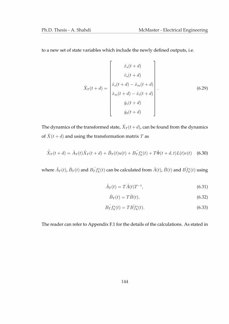
Ph.D. Thesis - A. Shahdi McMaster - Electrical Engineering
to a new set of state variables which include the newly defined outputs, i.e.
XT (t + d) =
xs(t + d)
vs(t + d)
xs(t + d)− xm(t + d)
xm(t + d)− xt(t + d)
y1(t + d)
y2(t + d)
. (6.29)
The dynamics of the transformed state, XT (t+d), can be found from the dynamics
of X(t + d) and using the transformation matrix T as
˙XT (t + d) = AT (t)XT (t + d) + BT (t)u(t) + ˆBT f ∗h(t) + T Φ(t + d, t)L(t)e(t) (6.30)
where AT (t), BT (t) and ˆBT f ∗h(t) can be calculated from A(t), B(t) and ˆBf ∗h(t) using
AT (t) = TA(t)T−1, (6.31)
BT (t) = TB(t), (6.32)
ˆBT f ∗h(t) = T ˆBf ∗h(t). (6.33)
The reader can refer to Appendix F.1 for the details of the calculations. As stated in
144

Ph.D. Thesis - A. Shahdi McMaster - Electrical Engineering
this appendix, the matrices AT (t), BT (t) and ˆBT f ∗h(t) have the following structures
AT (t) =
As(t) 0 0
0 Λ I
A1(t) A2(t) A3(t)
, (6.34)
BT (t) =
Bs(t)
0
By(t)
, (6.35)
ˆBT f ∗h(t) =
0
0
ˆBf ∗hy(t)
(6.36)
where
Λ =
−λ 0
0 −λ
(6.37)
and λ is defined in (6.27) and (6.28).
Assume the following control action
u(t) = B−1y (t)
(Ωy(t + d)− A1(t)XT1(t + d)− A2(t)XT2(t + d)
−A3(t)XT3(t + d)− ˆBf ∗hy(t)− T3Φ(t + d, t)L(t)e(t))
(6.38)
where T3 is a part of the transformation matrix T and is defined in (F.87), Ω is a
145
Ph.D. Thesis - A. Shahdi McMaster - Electrical Engineering
diagonal negative definite matrix in the form of
Ω =
−ω1 0
0 −ω2
, ω1, ω2 > 0 (6.39)
and
y(t + d) ,
y1(t + d)
y2(t + d)
. (6.40)
The inverse of the matrix By in (6.38) always exists due to its special structure as
shown in Appendix F.1. It is worth noticing that the control action in (6.38) is a
function of the parameter estimates, the calculated predicted state of the system
based on observations up to time t, X(t + d), and the state observation error, e(t).
Applying this control action to the open-loop dynamics in (6.30) results in the fol-
lowing closed-loop output dynamics
˙y(t + d) = Ωy(t + d). (6.41)
By substituting the control action from (6.38) into the system dynamics in (6.30),
one can obtain
˙XT (t + d) = ATcl
(t)XT (t + d) + ˆBf ∗hcl(t) + Tcl(t)Φ(t + d, t)L(t)e(t) (6.42)
146
Ph.D. Thesis - A. Shahdi McMaster - Electrical Engineering
where
ATcl(t) =
As(t)− Bs(t)B−1y (t)A1(t) −Bs(t)B
−1y (t)A2(t) −Bs(t)B
−1y (t)
(A3(t)− Ω
)
0 Λ I
0 0 Ω
,
(6.43)
ˆBf ∗hcl(t) =
−Bs(t)B−1y (t) ˆBf ∗hy(t)
0
0
(6.44)
and
Tcl(t) =
T1 − Bs(t)B−1y (t)T3
T2
0
. (6.45)
The definition of T1, T2 and T3 and the closed-loop matrices in (6.42) are given
in (F.87) and (F.90), respectively. It is worth mentioning that the eigenvalues of
the closed-loop state matrix, ATcl(t), vary with time. However as shown in Ap-
pendix F.2, these eigenvalues which are the union of the eigenvalues of the diago-
nal elements of the state matrix, will always have negative real parts. Nonetheless,
in the case of a time-varying system this is not sufficient to prove the stability of
the system.
147

Ph.D. Thesis - A. Shahdi McMaster - Electrical Engineering
6.5 System Stability and Parameters Adaptation Law
The dynamics of the state observation error, e(t), can be obtained by taking the
derivative of (6.8) and substituting X(t) and ˙X(t) from (6.3) and (6.10) as
e(t) =(A(t− d)− L(t)
)e(t) + A(t− d)X(t) + B(t− d)u(t− d) + ˜Bf ∗h(t− d) (6.46)
where the tilde variables represent the estimation errors, i.e. the error between the
actual and the estimated value of the corresponding variables
A = A− A, (6.47)
B = B − B, (6.48)
˜Bf ∗h = Bf∗hf ∗h − ˆBf ∗h . (6.49)
The user-defined observer gain L(t) is chosen to be
L(t) = A(t− d)−Υ (6.50)
where Υ < 0 is a constant matrix. Substituting L(t) from (6.50) in (6.46) results in
the following state observation error dynamics
e(t) = Υe(t) + A(t− d)X(t) + B(t− d)u(t− d) + ˜Bf ∗h(t− d). (6.51)
148

Ph.D. Thesis - A. Shahdi McMaster - Electrical Engineering
To facilitate the use of adaptive control, the dynamics of e(t) in (6.51) are rewritten
in an equivalent linear-in-parameter form as
e(t) = Υe(t) + Y (t)θ(t− d) (6.52)
where Y (t) is a regressor matrix which is a function of the measurements and θ(t)
is the vector of parameter estimation errors, i.e.
θ(t) = θ − θ(t). (6.53)
The system dynamics in linear-in-parameter form are presented in Appendix F.3. It
is important to mention that the vector of system parameters, θ, which includes the
user exogenous force, is assumed to be constant. Such assumption is shown to be
valid in experiments since the prediction horizon is relatively short with respect
to the rate of change in hand exogenous input. To remove the delay from the
estimation error vector, θ(t − d), as initially proposed by [113] a new signal, w(t),
is defined based on the following dynamics
w(t) = Υw(t)− Y (t)θ(t) + Y (t)θ(t− d). (6.54)
The signal w(t) will be added to the error signal e(t) resulting in the definition of a
new variable
r(t) , e(t) + w(t). (6.55)
149
Ph.D. Thesis - A. Shahdi McMaster - Electrical Engineering
Using (6.52) and (6.54), the dynamics of r(t) can be obtained as
r(t) = Υr(t) + Y (t)θ(t). (6.56)
A Lyapunov analysis is employed to prove the stability of the observation error
in (6.56) and to find the parameter adaptation law. The following theorem has
been utilized in the Lyapunov analysis.
Theorem 6.1: Consider a matrix Υ where all the eigenvalues have negative real
parts. For any matrix Q = QT > 0, there exists a unique matrix P = P T > 0 that
solves the following Lyapunov equation
ΥT P + PΥ = −Q. (6.57)
Proof: See [122].
Using the solution to the Lyapunov equation in (6.57), the following candidate
Lyapunov function is defined
V (t) =1
2rT (t)Pr(t) +
1
2θT (t)Γ−1θ(t) (6.58)
where Γ is a symmetric positive definite matrix, i.e. Γ = ΓT > 0. The derivative of
V (t) in (6.58) can be computed along the system state trajectory by replacing r(t)
from the dynamics equation in (6.56) as
V (t) =1
2rT (t)
(ΥT P + PΥ
)r(t) + rT (t)PY (t)θ(t) + ˙θT (t)Γ−1θ(t). (6.59)
150

Ph.D. Thesis - A. Shahdi McMaster - Electrical Engineering
Assuming that the actual parameters vector, θ, is constant and using the equa-
tion (6.53), the following projection based adaptation law is proposed
˙θi(t) = − ˙θi(t) =
0 θi ≤ θ−i
ΓTi Y T
i (t)P T r(t) θ−i ≤ θi ≤ θ+i
0 θ+i ≤ θi
(6.60)
where i denotes the ith parameter of the system, Γ is the parameter update gain,
and θ−i and θ+i represent the minimum and maximum allowable bounds on the pa-
rameter estimate θi. The application of this adaptation law results in the following
inequality for the sum of the last two terms on the right side of (6.59)
rT (t)PY (t)θ(t) + ˙θT (t)Γ−1θ(t) ≤ 0. (6.61)
Considering (6.57) and (6.61), it can be shown that
V (t) ≤ −1
2rT (t)Qr(t) < 0. (6.62)
It can be concluded from (6.58) and (6.62) that r(t) is bounded, i.e. r(t) ∈ L∞.
Moreover, by integrating (6.62) it can be shown that r(t) ∈ L2.
Theorem 6.2: The parameter estimation vector θ(t) converges to a constant value as
t →∞.
Proof: The proof is along the same lines as Theorem 2 in [113]. First it must be
shown that
rT (t)PY (t)θ(t) ∈ L1. (6.63)
151
Ph.D. Thesis - A. Shahdi McMaster - Electrical Engineering
This can be achieved by multiplying the dynamics of r(t) in (6.56) by rT (t)P from
left, integrating from 0 to t, and applying the boundedness of the Lyapunov func-
tion. Now consider the following derivative
d
dt
(1
2θT (t)Γ−1θ(t)
)= θT (t)Γ−1 ˙θ(t). (6.64)
Using the parameter adaptation law in (6.60), one can rewrite (6.64) as
d
dt
(1
2θT (t)Γ−1θ(t)
)= θT (t)Y T (t)P T r(t) (6.65)
and therefore for any arbitrary bounded k the following can be obtained
θT (t)Γ−1θ(t) = θT (t− k)Γ−1θ(t− k) + 2
∫ t
t−k
θT (s)Y T (s)P T r(t)ds. (6.66)
Given the fact that the operand of the integral in (6.66) is in L1 space as shown
in (6.63), for any finite k the following can be concluded
limt→∞
(θT (t)Γ−1θ(t)− θT (t− k)Γ−1θ(t− k)
)= 0, (6.67)
and therefore θ(t) converges to a constant value as t →∞.
Theorem 6.3: The error signal e(t) is bounded as a result of the boundedness of the
signal r(t).
Proof: To prove Theorem 6.3 the same steps as those in Lemma 4 of [113] should be
152
Ph.D. Thesis - A. Shahdi McMaster - Electrical Engineering
followed. The proof is based on the definition of r(t) in (6.55) and by showing that
limt→∞
w(t) = 0. (6.68)
This is achieved by demonstrating the dynamics of w(t) in (6.54) to satisfy the
following equation
w(t) = Υw(t) + L(t) + v(t) (6.69)
where the signals L(t) and v(t) satisfy
|L(t)| ≤ p(t)|wt| (6.70)
and
limt→∞
p(t) = 0, (6.71)
limt→∞
v(t) = 0. (6.72)
The norm of wt in (6.70) is defined as
|wt| = sup−d≤s≤0
|w(t + s)| (6.73)
Theorem 6.2 and the fact that the matrix Υ is Hurwitz are employed to obtain (6.69)-
(6.73). The reader is referred to [113] and the references within for the details of the
proof.
Lemma 6.1: A linear time-varying system with the state transition matrix A(t) is
stable if all the eigenvalues of A(t) always have negative real values and converge
153

Ph.D. Thesis - A. Shahdi McMaster - Electrical Engineering
to constant values as t →∞.
Proof: See [132].
Now consider the closed-loop dynamics in (6.42). The matrix ATcl(t) as stated
in Appendix F.2 satisfies all the conditions of Lemma 6.1. Using the boundedness
of e(t) and the estimated parameters of the system from Theorems 6.3 and 6.2,
respectively, it can be concluded that the dynamics equation in (6.42) represents
a stable system with bounded inputs. Hence, the vector of the states, XT (t + d),
is bounded. The boundedness of X(t + d) is concluded directly as a result of a
non-singular transformation T .
The control action, u(t), which is calculated using (6.38) depends only on X(t+
d) and e(t). By applying Theorem 6.3 and the boundedness of X(t + d), it can be
concluded that the control action is bounded. The boundedness of the states of
the system, X(t), can be shown as a result of the bounded inputs and the structure
of the teleoperation system which essentially consists of two mass-spring-damper
systems as stated in (4.20) and (4.23). As a result, the regressor matrix Y (t), which
comprises of system measurements and inputs, is bounded.
The second derivative of V (t) in (6.58) can be calculated as
V = −rT (t)Qr(t). (6.74)
By substituting r(t) from (6.56) on can write
V = −rT (t)Q(Υr(t) + Y (t)θ(t)
). (6.75)
154
Ph.D. Thesis - A. Shahdi McMaster - Electrical Engineering
Using the boundedness of r(t), Y (t) and θ(t) it can be concluded that V is also
bounded. Given the boundedness of V and (6.58) and by employing the Barbalat’s
Lemma [45] it can be proven that r(t) converges to zero. It is also straightforward
to show the convergence of the signal e(t) to zero as a result of w(t) going to zero.
6.5.1 Output Regulation
Consider the definition of the outputs in (6.27) and (6.28). These outputs can be
rewritten using the dynamics of X(t + d) in (6.25) as
y1(t + d) = X4(t + d) + λX3(t + d)
=˙
X3(t + d) + λX3(t + d)− Φ3(t + d, t)L(t)e(t), (6.76)
y2(t + d) = X6(t + d) + λX5(t + d)
=˙
X5(t + d) + λX5(t + d)− Φ5(t + d, t)L(t)e(t). (6.77)
The closed-loop output dynamics in (6.41) guarantee the convergence of y1(t + d)
and y2(t+d) to zero. Moreover since e(t) also converges to zero, it can be concluded
that
˙X3(t + d) + λX3(t + d) → 0, (6.78)
˙X5(t + d) + λX5(t + d) → 0 (6.79)
155

Ph.D. Thesis - A. Shahdi McMaster - Electrical Engineering
and therefore
X3(t + d) → 0, (6.80)
X5(t + d) → 0. (6.81)
It should be noted that delay-free transparent response can only be achieved if
the mapping between the current state of the system, X(t), and the predicted state,
X(t + d), is close to the actual mapping. The accuracy of this mapping directly de-
pends on the accuracy of parameter estimation. Several methods are proposed in
the following sections in order to enhance the parameter estimation performance.
In addition, perfect transparency requires the user and environment parameters,
including the user exogenous force to be constant. Changes in these parameters
may generate a transient error which would be corrected by the controller. The
decay rate of these transient errors can be increased by increasing the adaptation
gains. However, these gains can not be increased indefinitely due to the effect of
measurement noise and a finite sampling rate on system performance and stability.
6.6 Parameter Convergence and Composite Adaptive
Control
As mentioned earlier, achieving perfect tracking in time-delay teleoperation re-
quires the exact knowledge of the system parameters as well as the exogenous
inputs to the system. The tracking errors can be made smaller by increasing the
gain λ in (6.27) and (6.28). The parameter adaptation speed can also be increased
156
Ph.D. Thesis - A. Shahdi McMaster - Electrical Engineering
by increasing the gain Γ in (6.60). Although increasing these gains decrease the
bounds on the tracking errors, in practice noise amplification and instability due
to limited sampling rate limit these gains. As shown in Theorem 6.2 the parame-
ter estimates converge to constant values. However, these values may be different
from the actual system parameters. To converge to actual parameter values the
input signal requires to satisfy a certain condition, often referred to as persistency
of excitation in the adaptive control literature.
Consider the dynamics equation in (6.56). As proved in the last section, the
signal r(t) approaches zero as t → ∞. As a result the last term on the right hand
side of (6.56) goes to zero, i.e.
Y (t)θ(t) → 0. (6.82)
This however does not ensure that the parameter estimation error, θ(t), converges
to zero. The persistency of excitation condition [45] guarantees the convergence of
the parameter estimation errors to zero as t →∞. The details of this condition and
its proof are given in Appendix G.
6.6.1 Composite Adaptive Control
The parameter adaptation law in (6.60) utilizes the tracking error signal r(t) to es-
timate the system parameters. However, this is not the only source of information
available on the parameters. The hand and environment forces also contain valu-
able information on the parameters which can be used in parameter estimation. A
composite adaptation scheme will be utilized to use this extra source of informa-
tion in parameter adaptation. The application of the composite adaptive scheme
will result in a faster and more accurate parameter adaptation and consequently
157

Ph.D. Thesis - A. Shahdi McMaster - Electrical Engineering
smaller tracking errors.
Consider the linear second-order operator hand dynamics in (4.19). The error
between the actual and the estimated hand force can be written as
eh(t) = fh(t)− fh(t) (6.83)
where
fh(t) = f ∗h −mhxm(t)− bhxm(t)− khxm(t), (6.84)
fh(t) = f ∗h − mhxm(t)− bhxm(t)− khxm(t). (6.85)
To avoid the acceleration terms, filtered actual and estimated hand forces are being
used where the forces are passed through a first-order filter. The filtered error
between the actual and the estimated hand force can be calculated as
eh(t) = fh(t)− ¯fh(t) (6.86)
where
fh(t) = f ∗h −mh¯xm(t)− bh
¯xm(t)− khxm(t), (6.87)
¯fh(t) = f ∗h − mh
¯xm(t)− bh¯xm(t)− khxm(t). (6.88)
The filtered error eh in (6.86) can be written in the following linear-in-parameter
158
Ph.D. Thesis - A. Shahdi McMaster - Electrical Engineering
form
eh(t) =
(1 −¯xm(t) −¯xm(t) −xm(t)
)
f ∗h
mh
bh
kh
= Yh(t)θh(t) (6.89)
where tilde variables again represent the error between the actual and the estimated
parameters. Let the vector of hand parameters, θh, be written as a function of the
full vector of the system parameters, θ, as
θh = fh(θ). (6.90)
Note that fh(θ) is nonlinear since the elements of the system parameters vector,θ,
are nonlinear combinations of hand/environment parameters. This function is
presented in Appendix H and can be linearized around the estimated parameters
as
fh(θ) = fh(θ(t)) +∂fh
∂θ|θ=θ(t) (θ − θ(t)) + · · · . (6.91)
By ignoring the high order terms, (6.91) can be approximated as
θh(t) ' Jh(t)θ(t) (6.92)
where
Jh(t) =∂fh
∂θ|θ=θ(t) (6.93)
159

Ph.D. Thesis - A. Shahdi McMaster - Electrical Engineering
is given in Appendix H. Now from (6.89) and (6.92) the following can be derived
eh(t) ' Yh(t)Jh(t)θ(t). (6.94)
The same calculations can be performed for the error between the actual and
the estimated environment forces. Assuming a zero environment mass, one can
write
ee(t) = fe(t)− fe(t) (6.95)
where
fe(t) = bexs(t) + kexs(t), (6.96)
fe(t) = bexs(t) + kexs(t). (6.97)
The error ee(t) in (6.95) can be expressed in the following linear-in-parameter form
ee(t) =
(xs(t) xs(t)
)
be(t)
ke(t)
= Ye(t)θe(t). (6.98)
Using the similar calculations as in (6.90)-(6.93), the following can be obtained
ee(t) ' Ye(t)Je(t)θ(t) (6.99)
where Je(t) is given in Appendix H.
The composite parameter adaptation law can be derived by modifying the
160

Ph.D. Thesis - A. Shahdi McMaster - Electrical Engineering
adaptation law in (6.60) and by utilizing eh(t) and ee(t) as
˙θ(t) = ΓT
[Y T (t)P T r(t) + chJ
Th (t)Y T
h (t)eh(t) + ceJTe (t)Y T
e (t)ee(t)]
(6.100)
where ch > 0 and ce > 0 are the composite adaptation gains. These gains can be
used to increase or decrease the contribution of the hand and environment forces
estimation errors.
The next step is to show the stability of the system after utilizing the composite
adaptive scheme. Consider again the derivative of the Lyapunov function in (6.59).
Replacing ˙θ(t) from (6.100) results in
V (t) =1
2rT (t)
(ΥT P + PΥ
)r(t) + rT (t)PY (t)θ(t)
− (Y T (t)P T r(t) + chJ
Th (t)Y T
h (t)eh(t) + ceJTe (t)Y T
e (t)ee(t))T
θ(t) (6.101)
Using (6.57), this can be rewritten as
V (t) = −1
2rT (t)Qr(t)− (
chJTh (t)Y T
h (t)eh(t) + ceJTe (t)Y T
e (t)ee(t))T
θ(t) (6.102)
After substituting eh(t) and ee(t) from (6.94) and (6.99), one can write
V (t) = −1
2rT (t)Qr(t)
− θT (t)(chJ
Th (t)Y T
h (t)Yh(t)Jh(t) + ceJTe (t)Y T
e (t)Ye(t)Je(t))θ(t) (6.103)
161

Ph.D. Thesis - A. Shahdi McMaster - Electrical Engineering
Given that Q > 0 and ch and ce are positive scalars it can be concluded that
V (t) < 0 (6.104)
Hence the composite adaptation law stated in (6.100) stabilizes the time-delay tele-
operation system. It can also be shown that the signal r(t), the parameter estimate
errors, θ(t), as well as the system states, X(t), are bounded. As a result, the sec-
ond derivative of the Lyapunov function, V (t), will be bounded and employing
the Barbalat’s Lemma proves that V (t) goes to zero. From (6.103), it can then be
concluded that r(t) and θ(t) converge to zero as t →∞. In other words the param-
eter estimates will converge to their actual values. It is important to mention that
if the approximations in (6.94) and (6.99) are not accurate, i.e. the initial values of
the parameter estimates are far off the actual values, the parameter estimates can
potentially converge to values different than the actual parameters of the system.
6.7 Adaptive Control of Teleoperation with Time-varying
Delay
In the case of time-varying latencies, the dynamics of the teleoperation system can
be written in the following form
X(t) = AX(t) + Bu(t− d(t)) + Bf∗hf ∗h . (6.105)
162

Ph.D. Thesis - A. Shahdi McMaster - Electrical Engineering
For notational convenience, the argument of the control action in (6.105) is defined
as
m(t) , t− d(t). (6.106)
It is assumed that the argument is always increasing by time, i.e.
m(t) = 1− d(t) > 0 (6.107)
which leads to the following constraint on the time-varying time delay d(t)
d(t) < 1. (6.108)
Finally the inverse of m(·), which is also a function itself, is defined as
q(m(t)) = t. (6.109)
For the teleoperation system with time-varying delay as shown in (6.105), the
delay-reduced state is defined as
Z(t) = X(t) +
∫ t
m(t)
Φ(t, q(s))∂q(s)
∂sB(s)u(s)ds +
∫ t
m(t)
Φ(t, q(s))∂q(s)
∂sˆBf ∗h(s)ds
(6.110)
where m(·) and q(·) have been defined in (6.106) and (6.109) and X is the state of
an observer with the following dynamics
˙X(t) = A(m(t))X(t) + q(m(t))B(m(t))u(m(t)) + q(m(t)) ˆBf ∗h(m(t)) + L(t)e(t)
(6.111)
163

Ph.D. Thesis - A. Shahdi McMaster - Electrical Engineering
where e(t) is defined in (6.8). Note that
q(m(t)) =dq(s)
ds
∣∣∣∣s=m(t)
(6.112)
is different than ddtq(m(t)) which is equal to one according to (6.109).
The dynamics of the reduced system can be calculated by taking the derivative
of (6.110) as
˙Z(t) = ˙X(t) + Φ(t, q(t))q(t)B(t)u(t) + Φ(t, q(t))q(t) ˆBf ∗h(t)
− q(m(t))B(m(t))u(m(t))− q(m(t)) ˆBf ∗h(m(t))
+
∫ t
m(t)
∂
∂tΦ(t, q(s))
∂q(s)
∂sB(s)u(s)ds +
∫ t
m(t)
∂
∂tΦ(t, q(s))
∂q(s)
∂sˆBf ∗h(s)ds. (6.113)
Similar to (6.12), the estimated system transition matrix in the case of a time-
varying delay satisfies
∂Φ(t, s)
∂t= A(m(t))Φ(t, s) , Φ(s, s) = I (6.114)
Using (6.110) and (6.114), the dynamics of the reduced state can be written as
˙Z(t) = ˙X(t) + Φ(t, q(t))q(t)B(t)u(t) + Φ(t, q(t))q(t) ˆBf ∗h(t)
− q(m(t))B(m(t))u(m(t))− q(m(t)) ˆBf ∗h(m(t))
+ A(m(t))(Z(t)− X(t)
). (6.115)
164
Ph.D. Thesis - A. Shahdi McMaster - Electrical Engineering
By substituting ˙X from (6.111), one can write
˙Z(t) = A(m(t))Z(t)+Φ(t, q(t))q(t)B(t)u(t)+Φ(t, q(t))q(t) ˆBf ∗h(t)+L(t)e(t) (6.116)
The predicted state of the system is defined as
X(q(t)) , Φ(q(t), t)Z(t). (6.117)
Using this definition, the dynamics of the predicted state can be calculated using
˙X(q(t)) =
˙Φ(q(t), t)Z(t) + Φ(q(t), t)
˙Z(t). (6.118)
Following the similar steps as in (6.17)-(6.22), one can write
˙Φ(q(t), t) = q(t)A(t)Φ(q(t), t)− Φ(q(t), t)A(m(t)). (6.119)
Using (6.118), (6.119) and (6.116), the dynamics of the predicted state can be written
as
˙X(q(t)) =
(q(t)A(t)Φ(q(t), t)− Φ(q(t), t)A(m(t))
)Z(t)
+ Φ(q(t), t)(A(m(t))Z(t) + Φ(t, q(t))q(t)B(t)u(t)
+Φ(t, q(t))q(t) ˆBf ∗h(t) + L(t)e(t))
. (6.120)
Simplifying this equation and using (6.117) result in the following dynamics
˙X(q(t)) = q(t)A(t)X(q(t)) + q(t)B(t)u(t) + q(t) ˆBf ∗h(t) + Φ(q(t), t)L(t)e(t). (6.121)
165
Ph.D. Thesis - A. Shahdi McMaster - Electrical Engineering
Again new outputs are defined based on the predicted state of the system as
follows
y1(q(t)) , X4(q(t)) + λX3(q(t)) (6.122)
y2(q(t)) , X6(q(t)) + λX5(q(t)) (6.123)
where λ > 0 is a scalar. The predicted state of the system is transformed using the
same transformation as in (6.29). The dynamics of the transformed state, XT (q(t)),
can be calculated as
˙XT (q(t)) = q(t)AT (t)XT (q(t)) + q(t)BT (t)u(t) + q(t) ˆBT f ∗h(t) + T Φ(q(t), t)L(t)e(t).
(6.124)
where AT (t), BT (t) and ˆBT f ∗h(t) have exactly the same structure as those shown
in (6.34)-(6.37).
Consider the following control action
u(t) = B−1y (t)
(1
q(t)Ωy(q(t))− A1(t)XT1(q(t))− A2(t)XT2(q(t))
−A3(t)XT3(q(t))− ˆBf ∗hy(t)−1
q(t)T3Φ(q(t), t)L(t)e(t)
)(6.125)
where Ω is defined in (6.39). Substituting (6.125) into (6.124) results in the following
output dynamics
˙y(q(t)) = Ωy(q(t)). (6.126)
166

Ph.D. Thesis - A. Shahdi McMaster - Electrical Engineering
Moreover, the closed-loop dynamics of the transformed state in (6.124) can be writ-
ten as
˙XT (q(t)) = q(t)ATcl
(t)XT (q(t)) + q(t) ˆBf ∗hcl(t) + Tcl(t)Φ(q(t), t)L(t)e(t) (6.127)
where ATcl(t), ˆBf ∗hcl(t) and Tcl(t) are given in (6.43)-(6.45).
The dynamics of the state observation error can be obtained using (6.8), (6.105)
and (6.111) as
e(t) =(A(m(t))− L(t)
)e(t)+ A(m(t))X(t)+ B(m(t))u(m(t))+ ˜Bf ∗h(m(t)) (6.128)
where the tilde variables represent the error between the actual and the estimated
value of the corresponding variables. Choosing the gain L(t) as
L(t) = A(m(t))−Υ (6.129)
where Υ < 0 is a constant matrix results in the following observation error dynam-
ics
e(t) = Υe(t) + A(m(t))X(t) + B(m(t))u(m(t)) + ˜Bf ∗h(m(t)). (6.130)
These dynamics can be rewritten in linear-in-parameter form as
e(t) = Υe(t) + Y (t)θ(m(t)) (6.131)
Similar to (6.54) and to remove the delay from the observation error dynamics
167

Ph.D. Thesis - A. Shahdi McMaster - Electrical Engineering
in (6.134), a new signal w(t) with the following dynamics is defined
w(t) = Υw(t)− Y (t)θ(t) + Y (t)θ(m(t)). (6.132)
The signal w(t) will be added to the error signal e(t) resulting in the definition of a
new variable r(t)
r(t) , e(t) + w(t) (6.133)
with the following dynamics
r(t) = Υr(t) + Y (t)θ(t) (6.134)
These dynamics are exactly the same as those in (6.56). Hence the same Lyapunov
function can be utilized to prove the stability of the system and to derive the pa-
rameter adaptation law. These steps will not be repeated here in the interest of
space.
In case where the delay is constant, d(t) = d, the controller for the variable
delay will reduce to the one proposed for the constant delay case. For a constant
delay, one can write
m(t) = t− d, (6.135)
q(t) = t + d, (6.136)
and therefore
q(t) = q(m(t)) = 1. (6.137)
168
Ph.D. Thesis - A. Shahdi McMaster - Electrical Engineering
6.7.1 Practical Implementation Issues for the Time-varying Con-
troller in Packet Switched Networks
In the proposed controller for teleoperation with time-varying delay, it is assumed
that a model of time delay is available in the form of m(t) in (6.106), satisfying the
condition in (6.108). In practice, such model can be constructed numerically from a
real-time measurement of the round-trip delay. However, potential problems can
arise in a discrete-time implementation of the controller over a packet switched
network communication channel such as the Internet.
When the communication channel packet rate is similar to the sampling rate
at the receiving side and the delay is increasing, there will be a train of samples
with equal delay followed by one or more black-out samples. This is illustrated in
Fig. 6.2(a) where P1 represents the black-out period. During these black-out sam-
ples the latest received data packet could be used for control. However, the rate of
change of the delay, d(t), would be zero (delay is constant) for several samples and
it would be one for the black-out samples. This results in q(t) being zero and in-
finity, reflectively, which can cause problems in calculating the control action. This
issue can be partially remedied by having a faster sampling rate at the receiving
end than the packet rate of the channel as shown in Fig. 6.2(a). In this case, an
estimation of q(t) can be calculated since the packet arrival time is available to the
controller with a higher resolution. Note that such an assumption is indeed practi-
cal since the channel packet rate is often slower than the local controller sampling
rate.
In case where the delay is decreasing multiple packets may arrive within one
sample time in which case all but the most recent packet may be discarded. This
169

Ph.D. Thesis - A. Shahdi McMaster - Electrical Engineering
Figure 6.2: Communication over a packet switched network with (a) increasingdelay and (b) decreasing delay.
case is illustrated in Fig. 6.2(b) where P2 represents the period with more than one
received packets. Again, if similar sampling and packet rates are being employed
the model of the delay can not be constructed properly. Running the receiving
end model with faster sampling rate as shown in Fig. 6.2(b) can solve the prob-
lem by enabling the controller to calculate an estimate of q(t) using the available
information on packets arrival time.
Fig. 6.3 demonstrates how the proposed multi-rate solution can be implemented
in the case of our adaptive centralized control for time-delay teleoperation. As
shown in this figure, the control action calculations as well as the master/slave
170

Ph.D. Thesis - A. Shahdi McMaster - Electrical Engineering
Figure 6.3: Control action and master/slave devices running with a faster sam-pling rate than the communication packet transmission rate.
devices are operating with a higher sampling rate 1Tf
, while the communication
channel is running at a slower rate 1Ts
.
6.8 Experimental Results
Fig. 6.4 shows the schematic of the proposed adaptive predictive controller for a
general teleoperation system with time-varying delay. Assuming the centralized
controller resides at the master side, the slave control action and measurements are
subject to time-varying delays of τ1(t) and τ2(t) seconds. As mentioned previously,
the proposed adaptive control framework requires equal amount of latencies in
input channels and output channels. To accommodate for this, master control ac-
tion and measurements should be padded with τ1(t) and τ2(t) seconds of delay,
respectively.
The virtual tool position and velocity are generated using delayed hand and
environment force signals. These synthesized observations, along with the actual
observations, enter the model-based predictive controller block at the master site
171
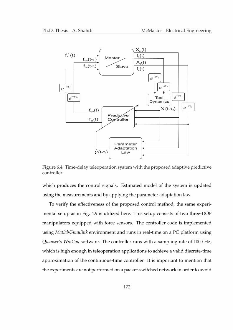
Ph.D. Thesis - A. Shahdi McMaster - Electrical Engineering
Figure 6.4: Time-delay teleoperation system with the proposed adaptive predictivecontroller
which produces the control signals. Estimated model of the system is updated
using the measurements and by applying the parameter adaptation law.
To verify the effectiveness of the proposed control method, the same experi-
mental setup as in Fig. 4.9 is utilized here. This setup consists of two three-DOF
manipulators equipped with force sensors. The controller code is implemented
using Matlab/Simulink environment and runs in real-time on a PC platform using
Quanser’s WinCon software. The controller runs with a sampling rate of 1000 Hz,
which is high enough in teleoperation applications to achieve a valid discrete-time
approximation of the continuous-time controller. It is important to mention that
the experiments are not performed on a packet-switched network in order to avoid
172
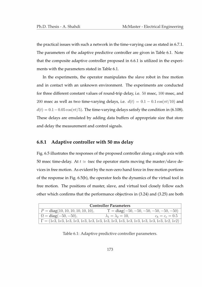
Ph.D. Thesis - A. Shahdi McMaster - Electrical Engineering
the practical issues with such a network in the time-varying case as stated in 6.7.1.
The parameters of the adaptive predictive controller are given in Table 6.1. Note
that the composite adaptive controller proposed in 6.6.1 is utilized in the experi-
ments with the parameters stated in Table 6.1.
In the experiments, the operator manipulates the slave robot in free motion
and in contact with an unknown environment. The experiments are conducted
for three different constant values of round-trip delay, i.e. 50 msec, 100 msec, and
200 msec as well as two time-varying delays, i.e. d(t) = 0.1 − 0.1 cos(πt/10) and
d(t) = 0.1− 0.05 cos(πt/5). The time-varying delays satisfy the condition in (6.108).
These delays are emulated by adding data buffers of appropriate size that store
and delay the measurement and control signals.
6.8.1 Adaptive controller with 50 ms delay
Fig. 6.5 illustrates the responses of the proposed controller along a single axis with
50 msec time-delay. At t ' 4sec the operator starts moving the master/slave de-
vices in free motion. As evident by the non-zero hand force in free motion portions
of the response in Fig. 6.5(b), the operator feels the dynamics of the virtual tool in
free motion. The positions of master, slave, and virtual tool closely follow each
other which confirms that the performance objectives in (3.24) and (3.25) are both
Controller ParametersP = diag(10, 10, 10, 10, 10, 10), Υ = diag(−50,−50,−50,−50,−50,−50)Ω = diag(−50,−50), λ1 = λ2 = 10, ch = ce = 0.5Γ = (1e3, 1e3, 1e3, 1e3, 1e3, 1e3, 1e3, 1e3, 1e3, 1e3, 1e3, 1e3, 1e3, 1e3, 1e3, 1e2, 1e2)
Table 6.1: Adaptive predictive controller parameters.
173
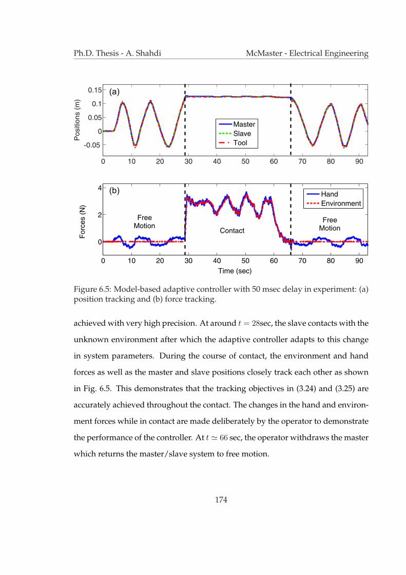
Ph.D. Thesis - A. Shahdi McMaster - Electrical Engineering
Figure 6.5: Model-based adaptive controller with 50 msec delay in experiment: (a)position tracking and (b) force tracking.
achieved with very high precision. At around t = 28sec, the slave contacts with the
unknown environment after which the adaptive controller adapts to this change
in system parameters. During the course of contact, the environment and hand
forces as well as the master and slave positions closely track each other as shown
in Fig. 6.5. This demonstrates that the tracking objectives in (3.24) and (3.25) are
accurately achieved throughout the contact. The changes in the hand and environ-
ment forces while in contact are made deliberately by the operator to demonstrate
the performance of the controller. At t ' 66 sec, the operator withdraws the master
which returns the master/slave system to free motion.
174
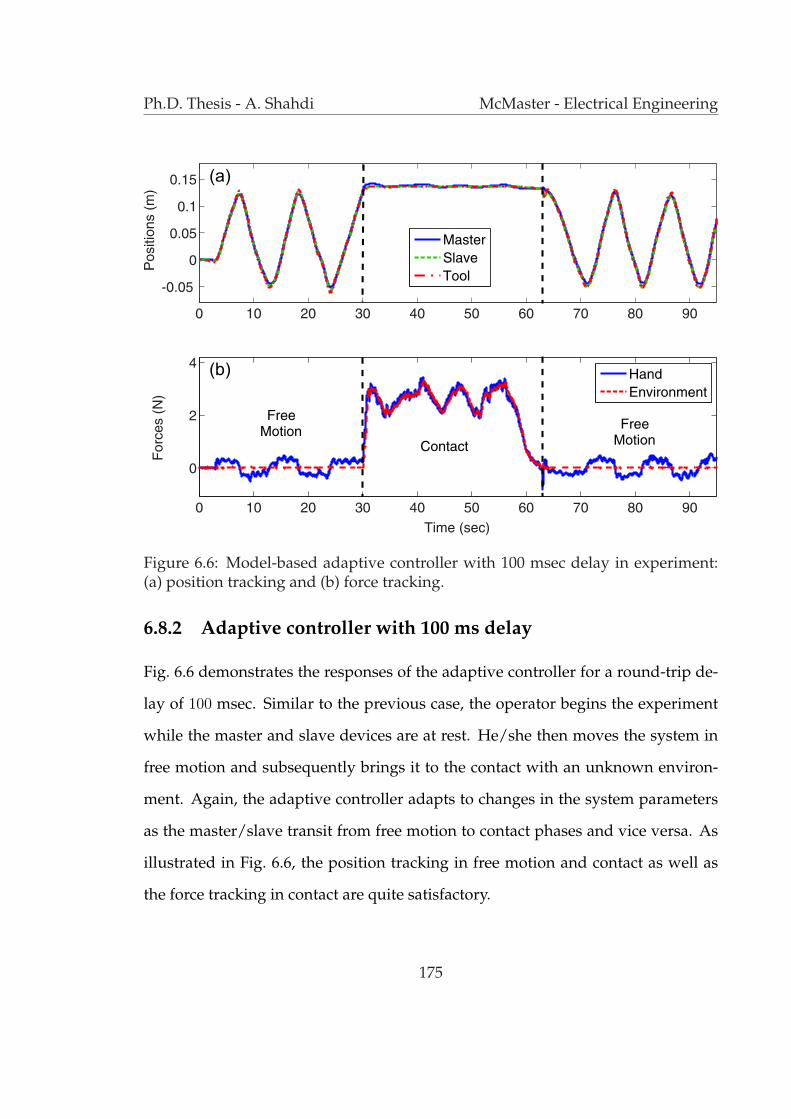
Ph.D. Thesis - A. Shahdi McMaster - Electrical Engineering
Figure 6.6: Model-based adaptive controller with 100 msec delay in experiment:(a) position tracking and (b) force tracking.
6.8.2 Adaptive controller with 100 ms delay
Fig. 6.6 demonstrates the responses of the adaptive controller for a round-trip de-
lay of 100 msec. Similar to the previous case, the operator begins the experiment
while the master and slave devices are at rest. He/she then moves the system in
free motion and subsequently brings it to the contact with an unknown environ-
ment. Again, the adaptive controller adapts to changes in the system parameters
as the master/slave transit from free motion to contact phases and vice versa. As
illustrated in Fig. 6.6, the position tracking in free motion and contact as well as
the force tracking in contact are quite satisfactory.
175
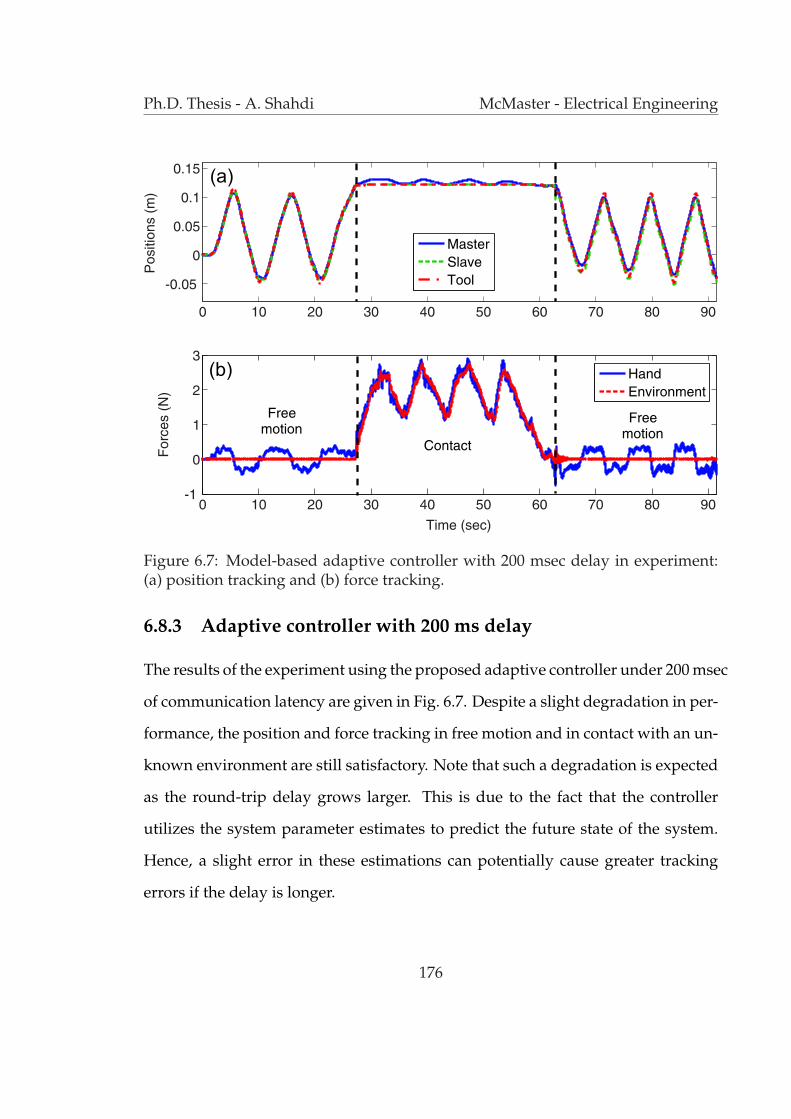
Ph.D. Thesis - A. Shahdi McMaster - Electrical Engineering
Figure 6.7: Model-based adaptive controller with 200 msec delay in experiment:(a) position tracking and (b) force tracking.
6.8.3 Adaptive controller with 200 ms delay
The results of the experiment using the proposed adaptive controller under 200 msec
of communication latency are given in Fig. 6.7. Despite a slight degradation in per-
formance, the position and force tracking in free motion and in contact with an un-
known environment are still satisfactory. Note that such a degradation is expected
as the round-trip delay grows larger. This is due to the fact that the controller
utilizes the system parameter estimates to predict the future state of the system.
Hence, a slight error in these estimations can potentially cause greater tracking
errors if the delay is longer.
176

Ph.D. Thesis - A. Shahdi McMaster - Electrical Engineering
6.8.4 Adaptive controller with time-varying delay
The experiments are repeated for two cases of time-varying delay. These delays
are calculated from the following equations
d1(t) = 0.1− 0.1 cos(πt/10), (6.138)
d2(t) = 0.1− 0.05 cos(πt/5). (6.139)
The second delay, d2(t), has a smaller range comparing to the first one but it
changes more rapidly. Similar to the cases with constant delay, the operator moves
the master/slave system in free motion and in contact with an unknown environ-
ment. Figs. 6.8 and 6.9 show the experimental results for the two cases of varying
time-delay. As is evident in these figures, the adaptive controller performs very
well in case of time-varying delay. Master, slave and virtual tool position track-
ing in free motion as well as hand and environment force tracking in contact with
the environment are all achieved with a high level of accuracy using the proposed
adaptive predictive controller. Also the transitions between the free motion and
contact phases are smooth and stable. The experiments with time-varying delays
were also repeated where the adaptive controller was designed for a constant time
delay. Delay values of 20, 100 and 200 msec were employed. The results showed
that the constant delay controller would become unstable if the actual delay is time
varying.
177
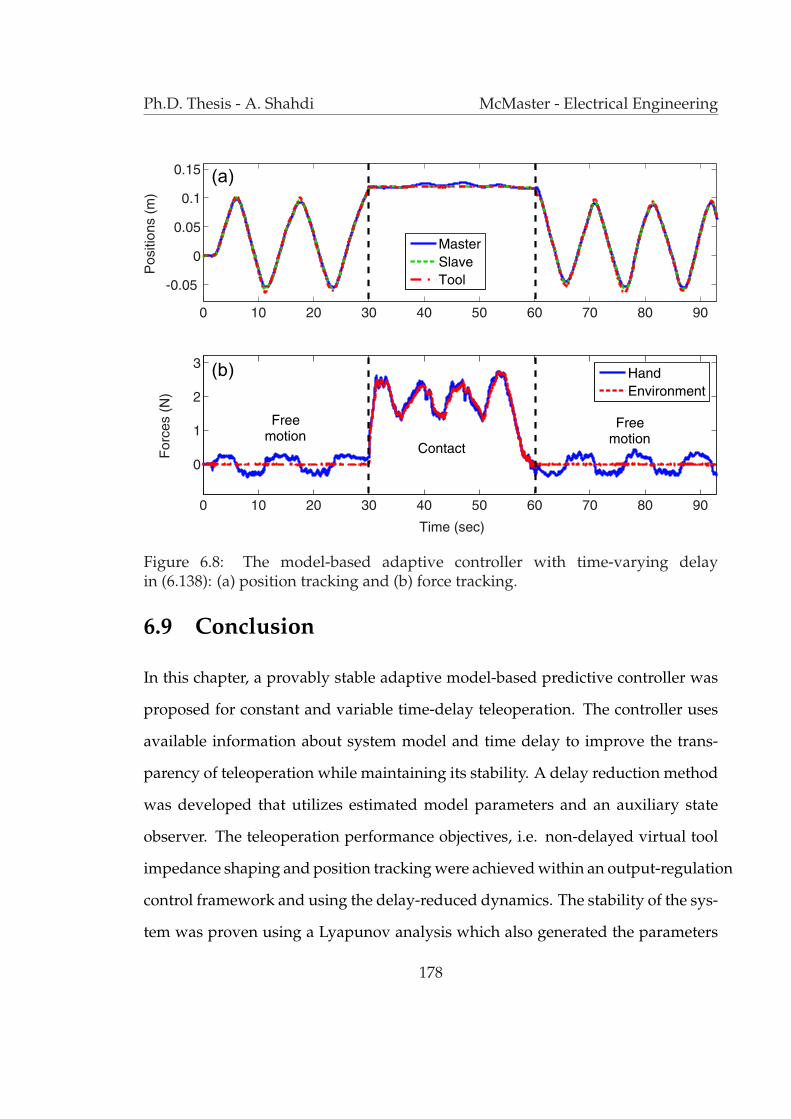
Ph.D. Thesis - A. Shahdi McMaster - Electrical Engineering
Figure 6.8: The model-based adaptive controller with time-varying delayin (6.138): (a) position tracking and (b) force tracking.
6.9 Conclusion
In this chapter, a provably stable adaptive model-based predictive controller was
proposed for constant and variable time-delay teleoperation. The controller uses
available information about system model and time delay to improve the trans-
parency of teleoperation while maintaining its stability. A delay reduction method
was developed that utilizes estimated model parameters and an auxiliary state
observer. The teleoperation performance objectives, i.e. non-delayed virtual tool
impedance shaping and position tracking were achieved within an output-regulation
control framework and using the delay-reduced dynamics. The stability of the sys-
tem was proven using a Lyapunov analysis which also generated the parameters
178
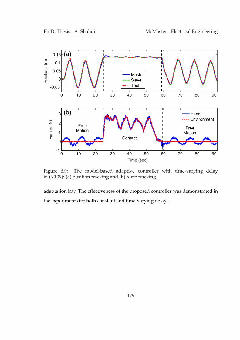
Ph.D. Thesis - A. Shahdi McMaster - Electrical Engineering
Figure 6.9: The model-based adaptive controller with time-varying delayin (6.139): (a) position tracking and (b) force tracking.
adaptation law. The effectiveness of the proposed controller was demonstrated in
the experiments for both constant and time-varying delays.
179

Chapter 7
Conclusions and Future Work
7.1 Conclusions
Time delay in communication channel and dynamic uncertainty are major barri-
ers to achieving transparency and robust stability in bilateral teleoperation. Most
existing teleoperation control techniques sacrifice transparency objectives in order
to gain robust stability in the presence of system uncertainty and communication
delay. The central idea of this thesis was to utilize available system model and
delay information in the controller in order to improve the stability-performance
trade-off in time-delay bilateral teleoperation. To this end, three new model-based
controllers were proposed and experimentally evaluated. These controllers were
designed to employ position and force measurements at both the master and slave
sites.
180

Ph.D. Thesis - A. Shahdi McMaster - Electrical Engineering
7.1.1 Model-based Decentralized Controller
First, a model-based decentralized controller was introduced that improved upon
on our earlier work on model-based time-delay teleoperation in [2]. In this con-
troller, master and slave measurements are used locally in the control of their re-
spective robots hence eliminating an extra delay from the loop that existed in the
controller of [2]. Teleoperation control was formulated as an output-feedback state-
space control problem incorporating performance objectives such as non-delayed
virtual tool impedance shaping, position tracking, and force tracking. To enable
the application of a decentralized control scheme, two output-delayed subsystems
at the master and slave site were considered in which local measurements are
delay-free whereas remote measurements are delayed. The application of a delay
reduction method and LQG-based sub-controllers to the reduced dynamics at the
master and slave sites resulted in a closed-loop dynamics with a state-delay pertur-
bation term. A delay-dependent frequency sweeping test was employed to analyze
the stability of these dynamics. Extensive robust stability and performance analy-
sis demonstrated that, using the same set of design parameters, the new decentral-
ized controller can provide enhanced performance and increased stability margins
when compared with its centralized counterpart in [2]. Experimental studies with
a single-axis teleoperation system also showed that the proposed approach is ef-
fective in improving teleoperation transparency under communication time delay.
181

Ph.D. Thesis - A. Shahdi McMaster - Electrical Engineering
7.1.2 Robust Controller
Mode-based predictive controllers can utilize the system model and the delay in-
formation to improve the transparency in time-delay bilateral teleoperation. How-
ever uncertainty in the system dynamics, particularly variations in the user and
environment dynamics can affect the robustness of such controllers. The use of a
multi-model control approach in the previous method proved effective in handling
uncertainties in the environment dynamics. Nevertheless, it is difficult to guaran-
tee the stability of such switching control strategy. Also, the number of modes
must increase if contact with a wide range of environments is considered which
further complicates the controller/switching strategy.
The second controller proposed in this thesis was a robust controller for time-
delay teleoperation. Through the use of local Lyapunov-based adaptive controllers,
the dynamics of the master and slave robots were linearized and rendered inde-
pendent from their parameters. However, uncertainty still existed in the form of
unknown linear operator and environment dynamics. Using the linearized dy-
namics, teleoperation control for achieving transparency and robust stability was
formulated as an H∞ robust control synthesis with multiple I/O delays. The re-
sulting problem was solved using decompositions into single-delay adobe-type
problems. The interaction between the local adaptive/nonlinear controllers and
the robust controller was fully accounted for in the proposed modeling and con-
trol synthesis.
The proposed approach explicitly incorporates information about model, de-
lay, and uncertainty into the design process and allows the designer to balance
182

Ph.D. Thesis - A. Shahdi McMaster - Electrical Engineering
transparency against robust stability through the selection of a set of design fil-
ters. Due to the use of local adaptive nonlinear controllers, modeling uncertainty
only appears in the form of perturbations in the user and environment parameters.
The ability to systematically optimize performance and stability trade-off in time-
delay teleoperation is rather unique to the proposed approach. This offers a real
advantage over existing methods that are often biased towards one of the conflict-
ing design requirements of performance or robust stability. The controller is also
distinct from the previous H∞ and µ-synthesis based teleoperation controllers in
that it can accommodate the nonlinear dynamics of the master and slave robots,
and more importantly, that it explicitly incorporates the delay into the design pro-
cess, providing an internal prediction mechanism. The results of performance and
stability analysis as well as experiments with a teleoperation setup demonstrated
the effectiveness of the proposed adaptive/robust controller.
7.1.3 Adaptive Controller
Although the proposed robust controller is less sensitive to modeling uncertainties,
it can still potentially sacrifice the performance of the system in favor of its robust
stability. This is due to the fact that a constant controller is employed through-
out all phases of teleoperation. The third proposed controller in this thesis was an
adaptive model-based predictive controller for constant and time-varying time-
delay teleoperation. This controller further improved on our earlier model-based
controllers by providing an adaptation mechanism to the user and environment
parameters within a provably stable framework. The proposed adaptive controller
183

Ph.D. Thesis - A. Shahdi McMaster - Electrical Engineering
could also handle both constant and time-varying delay in communication chan-
nel.
Unlike the majority of existing time-delay teleoperation controllers which sac-
rifice the performance of the system in favor of its stability, the new adaptive con-
troller uses available information about system model and time delay to improve
the transparency of teleoperation while maintaining its stability. In this process,
the estimates of the system parameters are updated by using the measurements.
A delay reduction method was developed that utilizes estimated model pa-
rameters and an auxiliary state observer to transform the system dynamics into
a delay-free form. The teleoperation performance objectives, i.e. non-delayed
virtual tool impedance shaping and position tracking were achieved within an
output-regulation control framework. The stability of the system was proven us-
ing a Lyapunov analysis which also generated the parameters adaptation law. The
effectiveness of the proposed controller was demonstrated through experimental
studies for both constant and variable time-delay.
7.2 Future Work
In future, research can be carried out to improve upon the proposed controllers in
this thesis. Some recommendations for future research are as follows:
• Decentralized Controller: The use of a multi-model control approach in the
proposed decentralized controller proved effective in handling environment
uncertainties. However, the stability of such switching control strategy must
184

Ph.D. Thesis - A. Shahdi McMaster - Electrical Engineering
be carefully investigated in future. Particularly, a formal analysis of the sta-
bility of the proposed switching control strategy can be performed.
• Robust Controller: Our original problem formulation in Fig. 5.2 was based
on a rather general model of the uncertainty considering passive ∆Zh/s and
∆Ze/s disturbances to the system dynamics. Such large uncertainties in the
system model could result in a conservative robust controller hence reducing
the transparency. This issue was partly addressed by restricting the uncer-
tainty to stiffness type variations in the environment dynamics. Also, the
problem could be aggravated by the fact that H∞ control framework would
disregard the structure of the uncertainty blocks. The use of µ-synthesis can
be investigated in order to account for the structure of the uncertainty in
the controller synthesis. Using D-K iterations, µ-synthesis method solves the
controller design problem by breaking it into a sequence of scaled H∞ syn-
thesis problems. In case of a time-delay system, each step can be solved using
the introduced adobe-based method in 5.4.
• Adaptive Controller: In the proposed adaptive controller, it was assumed
that the delay in all the input and output channels are equal. The controller
could be modified to remove this restriction as well as the need for extra
delay padding of the signals. Moreover, a decentralized version of the con-
troller may be developed in future. Such a controller can avoid the extra
delay that is imposed on the control loop by the centralized scheme. This
can potentially result in faster and more accurate adaptation which further
improves the transparency of teleoperation. Also, the implementation issues
concerning packet-switched networks can be investigated more thoroughly
185

Ph.D. Thesis - A. Shahdi McMaster - Electrical Engineering
and the proposed solutions in the thesis can be further developed, imple-
mented and experimentally verified.
Future work may also involve a comprehensive experimental comparison of
the performance of the proposed controllers with that of other existing time-delay
teleoperation controllers. In addition, the stability and the performance of the pro-
posed methods can be further tested by implementing the controllers on a multi-
axis teleoperation setup where the unmodeled dynamics and/or couplings among
the axes can potentially cause practical issues. Also, the effect of the improved
transparency on user performance in various time-delay teleoperation tasks can
be assessed by conducting human factors studies.
186

Appendix A
Master/Hand, Slave/Environment and
Tool Dynamics in State-space Form
The combined master and arm linearized dynamics in (4.27) can be written in the
following state-space form
xm(t)
vm(t)
=
0 1
− km+kh
mm+mh− bm+bh
mm+mh
xm(t)
vm(t)
+
0
1mm+mh
fcm(t)
+
0 0
1mm+mh
1mm+mh
f ∗h(t)
fcm(t)
(A.1)
187

Ph.D. Thesis - A. Shahdi McMaster - Electrical Engineering
xm(t)
fh(t)
=
1 0
mh(km+kh)mm+mh
− khmh(bm+bh)
mm+mh− bh
xm(t)
vm(t)
+
0
− mh
mm+mh
fcm(t)
+
0 0
1− mh
mm+mh− mh
mm+mh
f ∗h(t)
fcm(t)
+
υxm(t)
υfh(t)
. (A.2)
The state-space equivalents of the combined slave and compliant environment dy-
namics in (4.28) and for i = 1, 2 are as follows
xs(t)
vs(t)
=
0 1
− ks+σf ke
ms+σf me− bs+σf be
ms+σf me
xs(t)
vs(t)
+
0
1ms+σf me
fcs(t)
+
0 0
−σf
ms+σf me
1ms+σf me
f ∗e (t)
fcs(t)
(A.3)
xs(t)
fe(t)
=
1 0
σf me(ks+ke)
ms+me− σfke
σf me(bs+be)
ms+me− σfbe
xm(t)
vm(t)
+
0
− σf me
ms+σf me
·
fcs(t) +
0 0
−σf
(1− me
ms+me
)− σf me
ms+σf me
f ∗e (t)
fcs(t)
+
υxs(t)
υfe(t)
. (A.4)
In the case of contact with rigid environment, i.e. i = 3 in (4.28), the combined
slave and environment linearized dynamics can be written in the state-space form
188

Ph.D. Thesis - A. Shahdi McMaster - Electrical Engineering
as follows
xs(t)
vs(t)
=
0 1− σr
−(1− σr)ks
ms−(1− σr)
bs
ms
xs(t)
vs(t)
+
0
1−σr
ms
fcs(t)
+
0 0
0 1−σr
ms
f ∗e (t)
fcs(t)
(A.5)
xs(t)
fe(t)
=
1 0
0 0
xs(t)
vs(t)
+
0
σr
fcs +
0 0
0 σr
f ∗e (t)
fcs(t)
+
υxs(t)
υfe(t)
. (A.6)
The tool dynamics in (4.29) can also be presented in the state-space, i.e.
xt(t)
vt(t)
=
0 1
− kt
mt− bt
mt
xt(t)
vt(t)
+
0 0
1mt
− 1mt
fh(t)
fe(t)
(A.7)
yt(t) =
1 0
0 1
xt(t)
vt(t)
. (A.8)
189

Appendix B
Teleoperation Dynamics in Chapter 4
in State-space Form
B.1 Free Motion/Soft Contact
Based on the state definition in (4.31), the dynamics of the teleoperation in free
motion/soft contact in (4.32) can be presented in the following state-space form
xs(t)− xm(t)
vs(t)− vm(t)
xm(t)− xt(t)
vm(t)− vt(t)
xt(t)
vt(t)
=
0 1 0
− kse
mse− bse
mse− kse
mse+ kmh
mmh
0 0 0
− mekse
msemt+ ke
mt− mebse
msemt+ be
mt
− kmh
mmh− mekse
msemt+ ke
mt
−mhkmh
mmhmt+ kh
mt
· · ·
0 0 0
mekse
msemt− ke
mt
mebse
msemt− be
mt
mekse
msemt− ke
mt
+ mhkmh
mmhmt− kh
mt
190

Ph.D. Thesis - A. Shahdi McMaster - Electrical Engineering
0 0 0
− bse
mse+ bmh
mmh− kse
mse+ kmh
mmh− bse
mse+ bmh
mmh
1 0 0
· · · − bmh
mmh− mebse
msemt+ be
mt
− mhbmh
mmhmt+ bh
mt
− kmh
mmh− mekse
msemt+ ke
mt
−mhkmh
mmhmt+ kh
mt+ kt
mt
− bmh
mmh− mebse
msemt+ be
mt
− mhbmh
mmhmt+ bh
mt+ bt
mt
0 0 1
mebse
msemt− be
mt
+ mhbmh
mmhmt− bh
mt
mekse
msemt− ke
mt
+ mhkmh
mmhmt− kh
mt− kt
mt
mebse
msemt− be
mt
+ mhbmh
mmhmt− bh
mt− bt
mt
·
xs(t)− xm(t)
vs(t)− vm(t)
xm(t)− xt(t)
vm(t)− vt(t)
xt(t)
vt(t)
+
0 0
− 1mmh
1mse
0 0
1mmh
+ mh
mmhmt
me
msemt
0 0
− mh
mmhmt− me
msemt
fcm(t)
fcs(t)
+
0 0 0 0
− 1mmh
− 1mse
− 1mmh
1mse
0 0 0 0
1mmh
+ mh
mmhmt− 1
mt− me
msemt+ 1
mt
1mmh
+ mh
mmhmt
me
msemt
0 0 0 0
− mh
mmhmt+ 1
mt
me
msemt− 1
mt− mh
mmhmt− me
msemt
f ∗h(t)
f ∗e (t)
fcm(t)
fcs(t)
(B.9)
191

Ph.D. Thesis - A. Shahdi McMaster - Electrical Engineering
with the output equation
xm(t)
fh(t)
xs(t)
fe(t)
xt(t)
vt(t)
=
0 0 1 0 1
0 0 mhkmh
mmh− kh
mhbmh
mmh− bh
mhkmh
mmh− kh
1 0 1 0 1
−mekse
mse+ ke −mebse
mse+ be −mekse
mse+ ke −mebse
mse+ be −mekse
mse+ ke · · ·
0 0 0 0 1
0 0 0 0 0
0
mhbmh
mmh− bh
0
· · · −mebse
mse+ be
0
1
xs(t)− xm(t)
vs(t)− vm(t)
xm(t)− xt(t)
vm(t)− vt(t)
xt(t)
vt(t)
+
0 0 0 0
1− mh
mmh0 − mh
mmh0
0 0 0 0
0 1− me
mse0 me
mse
0 0 0 0
0 0 0 0
·
f ∗h(t)
f ∗e (t)
fcm(t)
fcs(t)
+
υxm(t)
υfh(t)
υxs(t)
υfe(t)
0
0
(B.10)
where αp in (4.31) is assumed to be equal to one. The state-space equations in free
motion/soft contact in (4.35) after the augmentation of f ∗h and f ∗h into the state
192

Ph.D. Thesis - A. Shahdi McMaster - Electrical Engineering
vector can be presented as
xs(t)− xm(t)
vs(t)− vm(t)
xm(t)− xt(t)
vm(t)− vt(t)
xt(t)
vt(t)
f ∗h(t)
f ∗h(t)
=
0 1 0
− kse
mse− bse
mse− kse
mse+ kmh
mmh
0 0 0
− mekse
msemt+ ke
mt− mebse
msemt+ be
mt
− kmh
mmh− mekse
msemt+ ke
mt
−mhkmh
mmhmt+ kh
mt
0 0 0 · · ·
mekse
msemt− ke
mt
mebse
msemt− be
mt
mekse
msemt− ke
mt
+ mhkmh
mmhmt− kh
mt
0 0 0
0 0 0
0 0 0
− bse
mse+ bmh
mmh− kse
mse+ kmh
mmh− bse
mse+ bmh
mmh
1 0 0
− bmh
mmh− mebse
msemt+ be
mt
− mhbmh
mmhmt+ bh
mt
− kmh
mmh− mekse
msemt+ ke
mt
−mhkmh
mmhmt+ kh
mt+ kt
mt
− bmh
mmh− mebse
msemt+ be
mt
− mhbmh
mmhmt+ bh
mt+ bt
mt
· · · 0 0 1 · · ·mebse
msemt− be
mt
+ mhbmh
mmhmt− bh
mt
mekse
msemt− ke
mt
+ mhkmh
mmhmt− kh
mt− kt
mt
mebse
msemt− be
mt
+ mhbmh
mmhmt− bh
mt− bt
mt
0 0 0
0 0 0
(B.11)
193

Ph.D. Thesis - A. Shahdi McMaster - Electrical Engineering
0 0
− 1mmh
0
0 0
1mmh
+ mh
mmhmt− 1
mt0
· · · 0 0
− mh
mmhmt+ 1
mt0
0 1
−α2fh −2αfh
xs(t)− xm(t)
vs(t)− vm(t)
xm(t)− xt(t)
vm(t)− vt(t)
xt(t)
vt(t)
f ∗h(t)
f ∗h(t)
+
0 0
− 1mmh
1mse
0 0
1mmh
+ mh
mmhmt
me
msemt
0 0
− mh
mmhmt− me
msemt
0 0
0 0
·
fcm(t)
fcs(t)
+
0 0 0 0
0 − 1mse
− 1mmh
1mse
0 0 0 0
0 − me
msemt+ 1
mt
1mmh
+ mh
mmhmt
me
msemt
0 0 0 0
0 me
msemt− 1
mt− mh
mmhmt− me
msemt
0 0 0 0
1 0 0 0
nf (t)
f ∗e (t)
fcm(t)
fcs(t)
(B.12)
194

Ph.D. Thesis - A. Shahdi McMaster - Electrical Engineering
where the output is given by
xm(t)
fh(t)
xs(t)
fe(t)
xt(t)
vt(t)
=
0 0 1 0 1
0 0 mhkmh
mmh− kh
mhbmh
mmh− bh
mhkmh
mmh− kh
1 0 1 0 1
−mekse
mse+ ke −mebse
mse+ be −mekse
mse+ ke −mebse
mse+ be −mekse
mse+ ke · · ·
0 0 0 0 1
0 0 0 0 0
0 0 0
mhbmh
mmh− bh 1− mh
mmh0
0 0 0
· · · −mebse
mse+ be 0 0
0 0 0
1 0 0
xs(t)− xm(t)
vs(t)− vm(t)
xm(t)− xt(t)
vm(t)− vt(t)
xt(t)
vt(t)
f ∗h(t)
f ∗h(t)
+
0 0 0 0
0 0 − mh
mmh0
0 0 0 0
0 1− me
mse0 me
mse
0 0 0 0
0 0 0 0
·
nf (t)
f ∗e (t)
fcm(t)
fcs(t)
+
υxm(t)
υfh(t)
υxs(t)
υfe(t)
0
0
. (B.13)
195
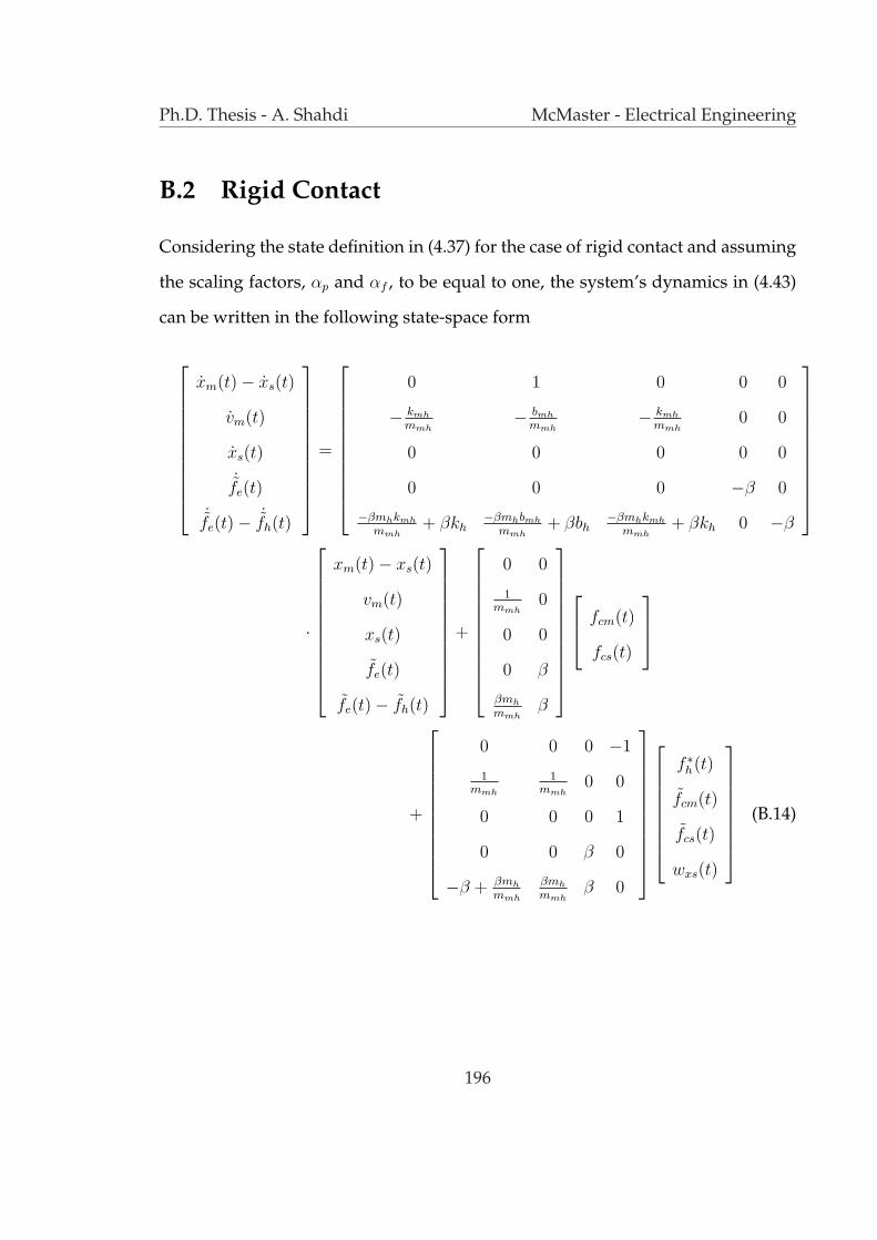
Ph.D. Thesis - A. Shahdi McMaster - Electrical Engineering
B.2 Rigid Contact
Considering the state definition in (4.37) for the case of rigid contact and assuming
the scaling factors, αp and αf , to be equal to one, the system’s dynamics in (4.43)
can be written in the following state-space form
xm(t)− xs(t)
vm(t)
xs(t)
˙fe(t)
˙fe(t)− ˙fh(t)
=
0 1 0 0 0
− kmh
mmh− bmh
mmh− kmh
mmh0 0
0 0 0 0 0
0 0 0 −β 0
−βmhkmh
mmh+ βkh
−βmhbmh
mmh+ βbh
−βmhkmh
mmh+ βkh 0 −β
·
xm(t)− xs(t)
vm(t)
xs(t)
fe(t)
fe(t)− fh(t)
+
0 0
1mmh
0
0 0
0 β
βmh
mmhβ
fcm(t)
fcs(t)
+
0 0 0 −1
1mmh
1mmh
0 0
0 0 0 1
0 0 β 0
−β + βmh
mmh
βmh
mmhβ 0
f ∗h(t)
fcm(t)
fcs(t)
wxs(t)
(B.14)
196

Ph.D. Thesis - A. Shahdi McMaster - Electrical Engineering
with the following output equation
xm(t)
fh(t)
xs(t)
fe(t)
=
1 0 1 0 0
mhkmh
mmh− kh
mhbmh
mmh− bh
mhkmh
mmh− kh 0 0
0 0 1 0 0
0 0 0 1 0
xm(t)− xs(t)
vm(t)
xs(t)
fe(t)
fe(t)− fh(t)
+
0 0
− mh
mmh0
0 0
0 0
fcm(t)
fcs(t)
+
0 0 0 0
1− mh
mmh− mh
mmh0 0
0 0 0 0
0 0 0 0
·
f ∗h(t)
fcm(t)
fcs(t)
wxs(t)
+
υxm(t)
υfh(t)
0
0
. (B.15)
197

Ph.D. Thesis - A. Shahdi McMaster - Electrical Engineering
After augmenting f ∗h and f ∗h into the state vector, the state-space equations in rigid
contact in (4.43) can be written as
xm(t)− xs(t)
vm(t)
xs(t)
˙fe(t)
˙fe(t)− ˙fh(t)
f ∗h(t)
f ∗h(t)
=
0 1 0 0 0
− kmh
mmh− bmh
mmh− kmh
mmh0 0
0 0 0 0 0
0 0 0 −β 0 · · ·−βmhkmh
mmh+ βkh
−βmhbmh
mmh+ βbh
−βmhkmh
mmh+ βkh 0 −β
0 0 0 0 0
0 0 0 0 0
0 0
1mmh
0
0 0
· · · 0 0
−β + βmh
mmh0
0 1
−α2fh −2αfh
xm(t)− xs(t)
vm(t)
xs(t)
fe(t)
fe(t)− fh(t)
f ∗h(t)
f ∗h(t)
+
0 0
1mmh
0
0 0
0 β
βmh
mmhβ
0 0
0 0
fcm(t)
fcs(t)
+
0 0 0 −1
0 1mmh
0 0
0 0 0 1
0 0 β 0
0 βmh
mmhβ 0
0 0 0 0
1 0 0 0
nf (t)
fcm(t)
fcs(t)
wxs(t)
(B.16)
198
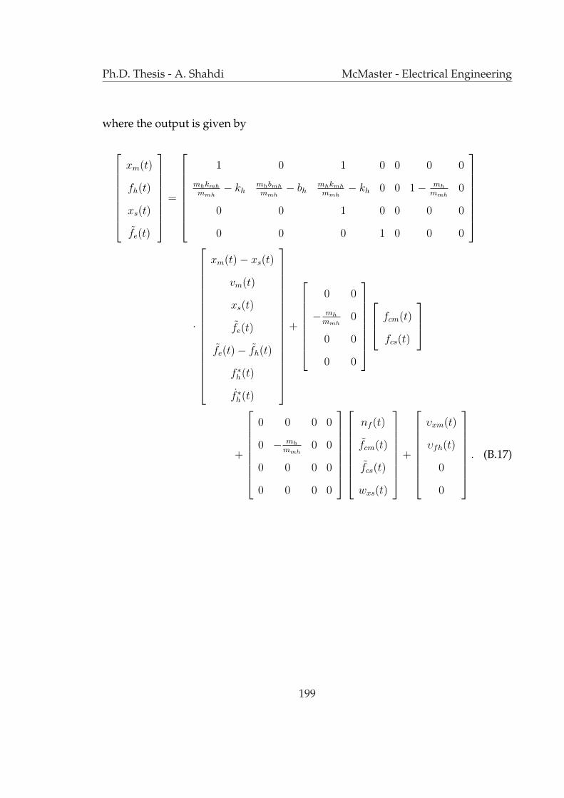
Ph.D. Thesis - A. Shahdi McMaster - Electrical Engineering
where the output is given by
xm(t)
fh(t)
xs(t)
fe(t)
=
1 0 1 0 0 0 0
mhkmh
mmh− kh
mhbmh
mmh− bh
mhkmh
mmh− kh 0 0 1− mh
mmh0
0 0 1 0 0 0 0
0 0 0 1 0 0 0
·
xm(t)− xs(t)
vm(t)
xs(t)
fe(t)
fe(t)− fh(t)
f ∗h(t)
f ∗h(t)
+
0 0
− mh
mmh0
0 0
0 0
fcm(t)
fcs(t)
+
0 0 0 0
0 − mh
mmh0 0
0 0 0 0
0 0 0 0
nf (t)
fcm(t)
fcs(t)
wxs(t)
+
υxm(t)
υfh(t)
0
0
. (B.17)
199

Appendix C
Proof of Theorem 4.1
C.1 Stabilizability
The controllability matrix of the original system with pair (A,B) can be written as
U =[B AB A2B · · · An−1B
]=
[B1 · · · BnI
|AB1 · · · ABnI| · · · |An−1B1 · · · An−1BnI
](C.18)
where the rank of U is
ρ(U) = nc ≤ n. (C.19)
200

Ph.D. Thesis - A. Shahdi McMaster - Electrical Engineering
Using the canonical decomposition theorem [122], there exists a transformation
X = PX , which transforms pair (A,B) to (A, B)
A = PAP−1 =
Ac A12
0 Ac
(C.20)
B = PB =
Bc
0
(C.21)
such that the pair (Ac, Bc) is controllable. The state transformation matrix P is
defined as
P−1 , Q = [q1 · · · qnc · · · qn] (C.22)
where q1 · · · qnc are nc linearly independent columns of matrix U and the last n−nc
columns are arbitrarily chosen vectors that make the matrix Q nonsingular. Since
the original system is assumed stabilizable, Ac would contain all unstable modes,
if any.
From (4.50), the controllability matrix of the transformed system represented
by the pair (Az, Bz) is given by
Uz =[Bz AzBz A2
zBz · · · An−1z Bz
]=
[e−Ahm1 B1 · · · e−Ahm
nI BnI|e−Ahm
1 AB1 · · · e−AhmnI ABnI
| · · ·
|e−Ahm1 An−1B1 · · · e−Ahm
nI An−1BnI] (C.23)
201
Ph.D. Thesis - A. Shahdi McMaster - Electrical Engineering
where the commutability of matrices A and e−Ah has been used. The following
lemma is needed to continue the proof.
Lemma A.1:
ρ(Uz) = ρ(U). (C.24)
Proof : Reordering the columns of a matrix will not alter its rank, so from (C.23)
ρ(Uz) = ρ([e−Ahm1
[B1 AB1 · · · An−1B1
] | · · ·
|e−AhmnI
[BnI
ABnI· · · An−1BnI
]]). (C.25)
Note that since e−Ahmj is a full rank square matrix, for each j,
ρ([e−Ahmj
[Bj ABj · · · AnI−1Bj
]]) = ρ (
[Bj ABj · · · AnI−1Bj
]). (C.26)
To proceed, we use the Caley-Hamilton theorem which states that each matrix sat-
isfies its own characteristic polynomial [122], i.e.
f(A) = anAn + an−1An−1 + · · ·+ a0 = 0 (C.27)
and therefore,
An = bn−1An−1 + · · ·+ b0 (C.28)
and consequently, all the powers of A greater than or equal to n can be written as
202

Ph.D. Thesis - A. Shahdi McMaster - Electrical Engineering
a linear combination of Ak, for k < n. Using this theorem and the Taylor series
expansion of e−Ahmj , one can write
e−Ahmj = c0I + c1A + c2A
2 + · · ·+ cn−1An−1. (C.29)
Using (C.29),
e−Ahmj AkBj = (c0I + c1A + c2A
2 + · · ·+ cn−1An−1)AkBj
= l0Bj + l1ABj + l2A2Bj + · · ·+ ln−1A
n−1Bj. (C.30)
Considering (C.26) and (C.30), one can conclude that for each j, [Bj ABj · · · An−1Bj]
and e−Ahmj [Bj ABj · · · An−1Bj] span the same space. Therefore, U and Uz are of the
same rank and the proof of Lemma A.1 is complete. Q.E.D.
The canonical form of the reduced system represented by the pair (Az, Bz) can
be generated using the same transformation P in (C.22) for the original system, i.e.
Az = PAzP−1 (C.31)
Bz = PBz or P−1Bz = Bz. (C.32)
Substituting Az and Bz from (4.50), results in
Az = PAP−1 =
Ac A12
0 Ac
(C.33)
203
Ph.D. Thesis - A. Shahdi McMaster - Electrical Engineering
P−1[b1z · · · bnI
z
]=
[e−Ahm
1 B1 · · · e−AhmnI BnI
]. (C.34)
For the jth column of (C.34), one can write
P−1bjz = e−Ahm
j Bj. (C.35)
Replacing e−Ahmj from (C.29)
P−1bjz = (c0I + c1A + c2A
2 + · · ·+ cn−1An−1)Bj. (C.36)
From the definition of P−1 in (C.22), the first nc columns of P−1 are the basis of the
controllability matrix U in (C.18). Considering (C.36), the right hand side of (C.34)
can be written in terms of first nc columns of P−1, i.e.
Bz =
Bcz nc
0
. (C.37)
Using (C.33) and (C.37), the controllability matrix of the pair (Az, Bz) can be writ-
ten as
Uz =
Bcz AcB
cz · · · An−1
c Bcz nc
0 0 · · · 0
. (C.38)
According to Lemma A.1, ρ(Uz) = ρ(U) = nc. Also, since the transformation P is
nonsingular, Uz and Uz have equal ranks, i.e.
ρ(Uz) = nc (C.39)
204
Ph.D. Thesis - A. Shahdi McMaster - Electrical Engineering
and consequently, the pair (Ac, Bcz) is controllable where Ac contains all the unsta-
ble poles.
C.2 Detectability
The proof follows the same lines as in the case of stabilizability. The observability
matrix of the original system (A,B) can be written as
V =
C
CA
CA2
...
CAn−1
=
C1
...
CnO
−−C1A
...
CnOA
−−...
−−C1A
n−1
...
CnOAn−1
(C.40)
where the rank of V is
ρ(V ) = nob ≤ n. (C.41)
205

Ph.D. Thesis - A. Shahdi McMaster - Electrical Engineering
Using the canonical decomposition theorem [122], there exists a transformation
X = PX , which transforms pair (A,C) to (A, C)
A = PAP−1 =
Ao 0
A21 Ao
(C.42)
C = CP−1 =
[Co 0
](C.43)
and the pair (Ao, Co) is observable. The matrix P is defined as
P ,
r1
...
rno
...
rn
(C.44)
where r1 · · · rnob are nob independent rows of V and the last n − nob rows are ar-
bitrarily chosen vectors such that the matrix P is nonsingular. The detectability
of the original system requires all unstable modes to be observable. Therefore, Ao
should contain all unstable modes. The canonical representation of the reduced
system (Az, Cz) can be obtained using transformation P in (C.44) from the original
system as
Az = PAzP−1 (C.45)
206
Ph.D. Thesis - A. Shahdi McMaster - Electrical Engineering
Cz = CzP−1 or CzP = Cz. (C.46)
Substituting Az and Cz from (4.50) and (4.56), results in
Az = PAP−1 =
Ao 0
A21 Ao
(C.47)
C1z
...
CnOz
P =
C1eAdm1
o
C2eAdm2
o
...
CnoeAdmno
o
. (C.48)
For the jth row of (C.48), one can write
CjzP = Cje
AdmjO . (C.49)
Using the Caley-Hamilton theorem,
CjzP = Cj(a0I + a1A + a2A
2 + · · ·+ an−1An−1). (C.50)
From the definition of P in (C.44), the first nob rows of P are the basis of matrix V
in (C.40). Therefore, the right hand side of (C.48) can be written in terms of the first
nob rows of P , i.e.
Cz =
[Co
z 0
]. (C.51)
207

Ph.D. Thesis - A. Shahdi McMaster - Electrical Engineering
Using (C.47) and (C.51), the observability matrix of the pair (Az, Cz) can be written
as
Vz =
Coz 0
Coz Ao 0
...
Coz A
n−1o 0
. (C.52)
Using the dual arguments of Lemma A.1, ρ(Vz) = nob, and hence the pair (Ao, Coz )
is observable. Also from the canonical decomposition theorem, Ao encompasses
all unstable poles. Consequently, the reduced system is detectable. Q.E.D.
208

Appendix D
One-block Equivalent of a Four-block
Time-delay Problem
This appendix discusses the details of reducing a time-delay four-block problem
in (5.46) and (5.48) to the equivalent one-block problem using the solution to the
problem where the delay is ignored. The following are the conditions that need to
be satisfied for the delay-free problem to have a solution [35]
maxγz, γw < γ (D.53)
HX ∈ dom Ric , X , Ric(HX) ≥ 0 (D.54)
HY ∈ dom Ric , Y , Ric(HY ) ≥ 0 (D.55)
ρ(XY ) < γ (D.56)
209

Ph.D. Thesis - A. Shahdi McMaster - Electrical Engineering
where
γz ,‖ (I −D12(D′12D12)
−1D′12)D11 ‖
γw ,‖ D11(I −D′21(D21D
′21)
−1D21) ‖ (D.57)
and
HX ,
A 0
−C ′1C1 −A′
−
B1 B2
−C ′1D11 −C ′
1D12
×
D′11D11 − γ2I D′
11D12
D′12D11 D′
12D12
−1
D′11C1 B′
1
D′12C1 B′
2
(D.58)
HY ,
A′ 0
−B1B′1 −A
−
C ′1 C ′
2
−B1D′11 −B1D
′21
×
D11D′11 − γ2I D11D
′21
D21D′11 D21D
′21
−1
D11B′1 C1
D21B′1 C2
. (D.59)
Assuming
Θz ,
D′11D11 − γ2I D′
11D12
D′12D11 D′
12D12
(D.60)
Θw ,
D11D′11 − γ2I D11D
′21
D21D′11 D21D
′21
(D.61)
210
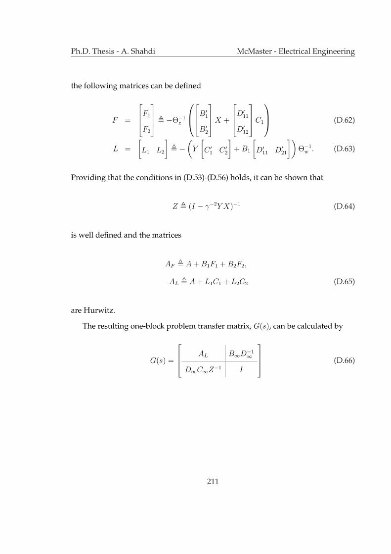
Ph.D. Thesis - A. Shahdi McMaster - Electrical Engineering
the following matrices can be defined
F =
F1
F2
, −Θ−1
z
B′1
B′2
X +
D′11
D′12
C1
(D.62)
L =
[L1 L2
], −
(Y
[C ′
1 C ′2
]+ B1
[D′
11 D′21
])Θ−1
w . (D.63)
Providing that the conditions in (D.53)-(D.56) holds, it can be shown that
Z , (I − γ−2Y X)−1 (D.64)
is well defined and the matrices
AF , A + B1F1 + B2F2,
AL , A + L1C1 + L2C2 (D.65)
are Hurwitz.
The resulting one-block problem transfer matrix, G(s), can be calculated by
G(s) =
AL B∞D−1∞
D∞C∞Z−1 I
(D.66)
211
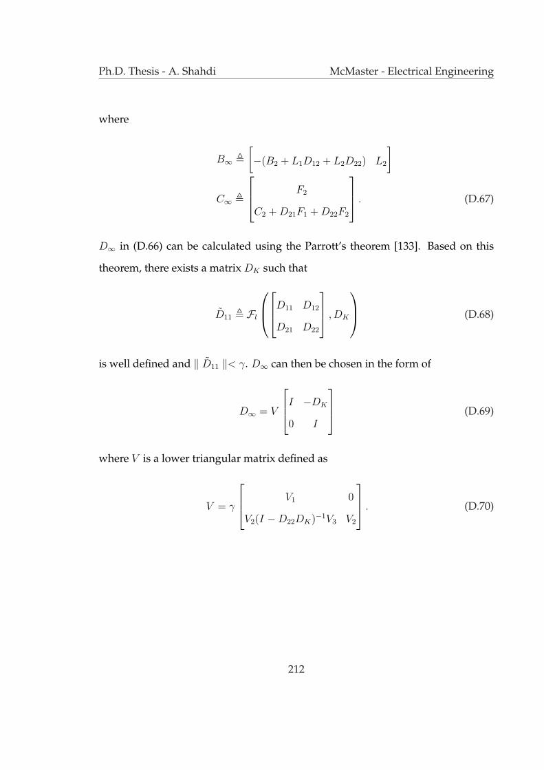
Ph.D. Thesis - A. Shahdi McMaster - Electrical Engineering
where
B∞ ,[−(B2 + L1D12 + L2D22) L2
]
C∞ ,
F2
C2 + D21F1 + D22F2
. (D.67)
D∞ in (D.66) can be calculated using the Parrott’s theorem [133]. Based on this
theorem, there exists a matrix DK such that
D11 , Fl
D11 D12
D21 D22
, DK
(D.68)
is well defined and ‖ D11 ‖< γ. D∞ can then be chosen in the form of
D∞ = V
I −DK
0 I
(D.69)
where V is a lower triangular matrix defined as
V = γ
V1 0
V2(I −D22DK)−1V3 V2
. (D.70)
212
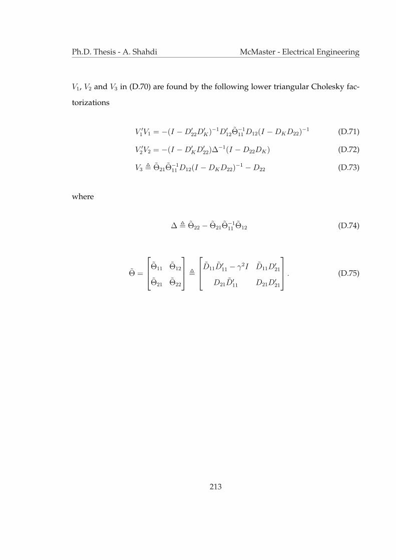
Ph.D. Thesis - A. Shahdi McMaster - Electrical Engineering
V1, V2 and V3 in (D.70) are found by the following lower triangular Cholesky fac-
torizations
V ′1V1 = −(I −D′
22D′K)−1D′
12Θ−111 D12(I −DKD22)
−1 (D.71)
V ′2V2 = −(I −D′
KD′22)∆
−1(I −D22DK) (D.72)
V3 , Θ21Θ−111 D12(I −DKD22)
−1 −D22 (D.73)
where
∆ , Θ22 − Θ21Θ−111 Θ12 (D.74)
Θ =
Θ11 Θ12
Θ21 Θ22
,
D11D′11 − γ2I D11D
′21
D21D′11 D21D
′21
. (D.75)
213
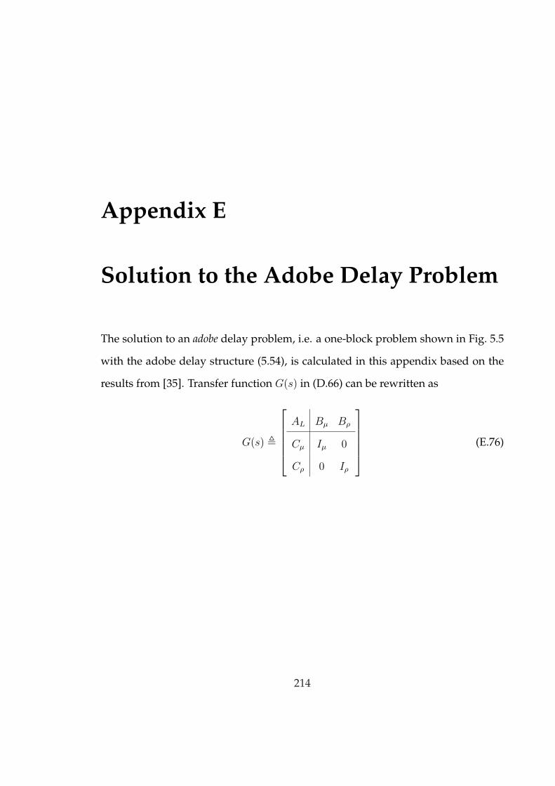
Appendix E
Solution to the Adobe Delay Problem
The solution to an adobe delay problem, i.e. a one-block problem shown in Fig. 5.5
with the adobe delay structure (5.54), is calculated in this appendix based on the
results from [35]. Transfer function G(s) in (D.66) can be rewritten as
G(s) ,
AL Bµ Bρ
Cµ Iµ 0
Cρ 0 Iρ
(E.76)
214
Ph.D. Thesis - A. Shahdi McMaster - Electrical Engineering
where G(s) is partitioned compatibly with the adobe delay structure in (5.54). Let
J ,
Inu 0
0 −Iny
Jµ ,[
Iµ 0
]J
Iµ
0
Jρ ,[
0 Iρ
]J
0
Iρ
. (E.77)
Define Σ(t) as
Σ(t) =
Σ11(t) Σ12(t)
Σ21(t) Σ22(t)
, eHt (E.78)
and the Hamiltonian matrix H as
H =
H11(t) H12(t)
H21(t) H22(t)
,
AL −BρCρ −BρJρB′ρ
−C ′µJµBµ −A′
L + C ′ρB
′ρ
. (E.79)
The adobe delay problem has a solution if and only if Σ22(t) is nonsingular for
∀t ∈ [0, h]. The controller K can then be obtained by
K = Cr
I 0
Π I
G−1, Q
(E.80)
215
Ph.D. Thesis - A. Shahdi McMaster - Electrical Engineering
where
G(s) =
AL Σ′22Bµ + Σ′
12C′µJµ Bρ
CµΣ′−122 Iµ 0
Cρ − JρB′ρΣ
−122 Σ21 0 Iρ
(E.81)
is a bistable transfer matrix and
Π(s) = πh
e−hs
H11 H12 Bρ
H21 H22 −C ′µJµ
Cρ JρB′ρ 0
(E.82)
is a FIR operator. Q in (E.80) is a contractive matrix and Σ = Σ(h).
The completion operator, πh in (E.82), is defined as follows [109]. Assuming a
h-delayed system, e−hsP , with
P =
A B
C 0
(E.83)
the completion operator is calculated by
πh(e−hsP ) =
A B
Ce−Ah 0
− e−hs
A B
C 0
. (E.84)
216

Appendix F
Teleoperation Dynamics in Chapter 6
in State-space Form
Based on the state definition in (6.2), the dynamics of the teleoperation system
in (6.3) can be presented in the following state-space form
xs(t)
vs(t)
xs(t)− xm(t)
vs(t)− vm(t)
xm(t)− xt(t)
vm(t)− vt(t)
=
0 1 0
− ke
ms− bse
ms0
0 0 0
− ke
ms+ kh
mmh− bse
ms+ bmh
mmh− kh
mmh· · ·
0 0 0
− kh
mmh+ kt
mt
ke
mt
− mhkh
mmhmt+ kh
mt
− bmh
mmh+ bt
mt
be
mt
− mhbmh
mmhmt+ bh
mt
kh
mmh− kt
mt
mhkh
mmhmt− kh
mt
(F.85)
217

Ph.D. Thesis - A. Shahdi McMaster - Electrical Engineering
0 0 0
0 0 0
1 0 0
· · · − bmh
mmh0 0
0 0 1
bmh
mmh− bt
mt
mhbmh
mmhmt− bh
mt
− kt
mt− bt
mt
xs(t)
vs(t)
xs(t)− xm(t)
vs(t)− vm(t)
xm(t)− xt(t)
vm(t)− vt(t)
+
0 0
1ms
0
0 0
1ms
− 1mmh
0 0
0 1mmh
+ mh
mmhmt
fcs(t− d(t))
fcm(t− d(t))
+
0
0
0
− 1mmh
0
1mmh
− 1mt
+ mh
mmhmt
f ∗h (F.86)
Note that in these state-space equations the environment mass, me, and the master
and slave stiffnesses, km and ks, are assumed to be zero.
218
Ph.D. Thesis - A. Shahdi McMaster - Electrical Engineering
F.1 Teleoperation Dynamics after Transformation
After applying the non-singular transformation
T =
1 0 0 0 0 0
0 1 0 0 0 0
0 0 1 0 0 0
0 0 0 0 1 0
0 0 λ 1 0 0
0 0 0 0 λ 1
,
T1
T2
T3
(F.87)
where λ is defined in (6.27) and (6.28), the dynamics of the transformed state
in (6.30) can be written in the following form
219

Ph.D. Thesis - A. Shahdi McMaster - Electrical Engineering
˙xs(t + d)
˙vs(t + d)
˙xs(t + d)− ˙xm(t + d)
˙xm(t + d)− ˙xt(t + d)
˙y1(t + d)
˙y2(t + d)
=
0 1
− ke
ms− bse
ms
0 0
0 0 · · ·− ke
ms+ kh
mmh− bse
ms+ bmh
mmh
− kh
mmh+ kt
mt+ ke
mt
− mhkh
mmhmt+ kh
mt
− bmh
mmh+ bt
mt+ be
mt
− mhbmh
mmhmt+ bh
mt
0 0 0 0
0 0 0 0
· · · −λ 0 1 0
0 −λ 0 1
− kh
mmh+ λ bmh
mmh− λ2 0 − bmh
mmh+ λ 0
kh
mmh− kt
mt− λ bmh
mmh+ λ bt
mt
mhkh
mmhmt− kh
mt− λ mhbmh
mmhmt+ λ bh
mt
− kt
mt+ λ bt
mt− λ2
bmh
mmh− bt
mt
mhbmh
mmhmt− bh
mt
− bt
mt+ λ
·
xs(t + d)
vs(t + d)
xs(t + d)− xm(t + d)
xm(t + d)− xt(t + d)
y1(t + d)
y2(t + d)
+
0 0
1ms
0
0 0
0 0
1ms
− 1mmh
0 1mmh
+ mh
mmhmt
fcs(t)
fcm(t)
220
Ph.D. Thesis - A. Shahdi McMaster - Electrical Engineering
+
0
0
0
0
− 1mmh
1mmh
− 1mt
+ mh
mmhmt
f ∗h + T Φ(t + d, t)L(t)e(t). (F.88)
By(t) in (6.35) which is defined as the last two rows of BT (t) in (6.30) is in the
following form
By(t) =
1ms
− 1mmh
0 1mmh
+ mh
mmhmt
. (F.89)
Because the masses in (F.89) are non-zero the determinant of the matrix By(t) is
always non-zero and therefore this matrix is always invertible.
221

Ph.D. Thesis - A. Shahdi McMaster - Electrical Engineering
F.2 Teleoperation Dynamics in Chapter 6 in Closed-
loop Form
The closed-loop dynamics in (6.42) can be stated in the following state-space form
˙xs(t + d)
˙vs(t + d)
˙xs(t + d)− ˙xm(t + d)
˙xm(t + d)− ˙xt(t + d)
˙y1(t + d)
˙y2(t + d)
=
0 1 0
−kteh
mth− bteh
mth
kth
mth− λ bth
mth+ λ2
0 0 −λ
0 0 0 · · ·0 0 0
0 0 0
0 0 0
kt
mth− λ bt
mth+ λ2 mt
mth
bth
mth− λ− ω1
bt
mth− λ mt
mth− ω2
mt
mth
0 1 0
· · · −λ 0 1
0 −ω1 0
0 0 −ω2
·
xs(t + d)
vs(t + d)
xs(t + d)− xm(t + d)
xm(t + d)− xt(t + d)
y1(t + d)
y2(t + d)
+
0
1mth
0
0
0
0
f ∗h
222
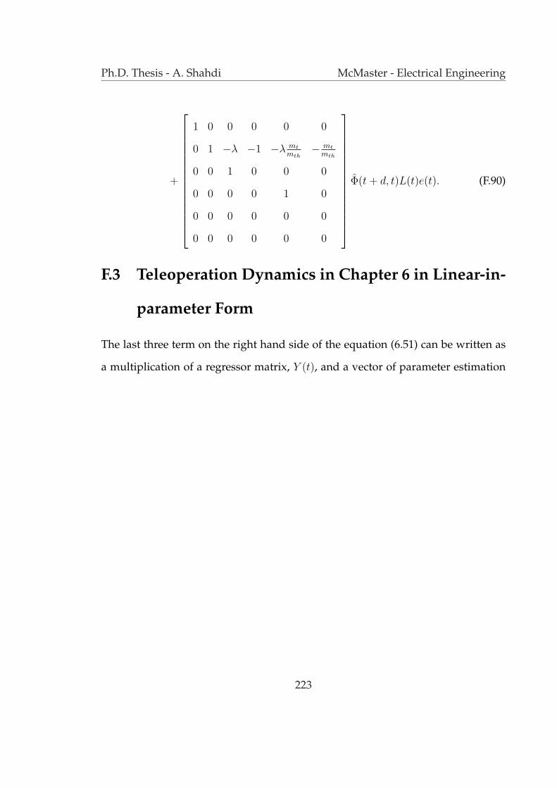
Ph.D. Thesis - A. Shahdi McMaster - Electrical Engineering
+
1 0 0 0 0 0
0 1 −λ −1 −λ mt
mth− mt
mth
0 0 1 0 0 0
0 0 0 0 1 0
0 0 0 0 0 0
0 0 0 0 0 0
Φ(t + d, t)L(t)e(t). (F.90)
F.3 Teleoperation Dynamics in Chapter 6 in Linear-in-
parameter Form
The last three term on the right hand side of the equation (6.51) can be written as
a multiplication of a regressor matrix, Y (t), and a vector of parameter estimation
223
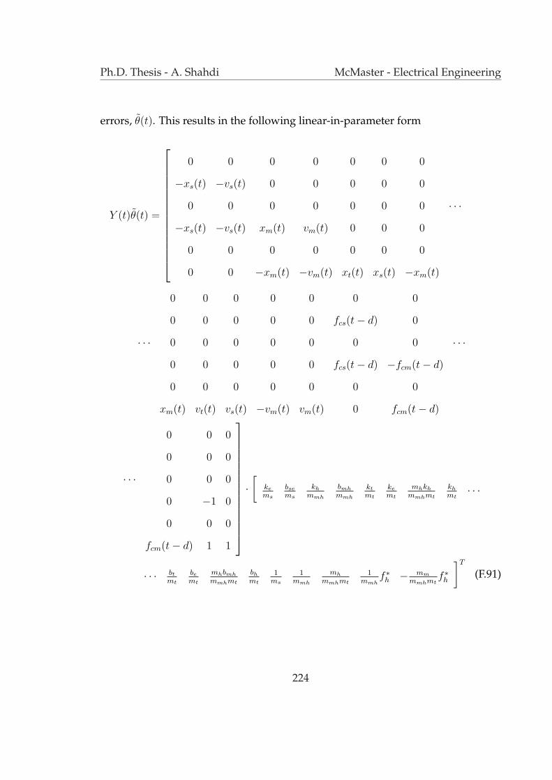
Ph.D. Thesis - A. Shahdi McMaster - Electrical Engineering
errors, θ(t). This results in the following linear-in-parameter form
Y (t)θ(t) =
0 0 0 0 0 0 0
−xs(t) −vs(t) 0 0 0 0 0
0 0 0 0 0 0 0 · · ·−xs(t) −vs(t) xm(t) vm(t) 0 0 0
0 0 0 0 0 0 0
0 0 −xm(t) −vm(t) xt(t) xs(t) −xm(t)
0 0 0 0 0 0 0
0 0 0 0 0 fcs(t− d) 0
· · · 0 0 0 0 0 0 0 · · ·0 0 0 0 0 fcs(t− d) −fcm(t− d)
0 0 0 0 0 0 0
xm(t) vt(t) vs(t) −vm(t) vm(t) 0 fcm(t− d)
0 0 0
0 0 0
· · · 0 0 0
0 −1 0
0 0 0
fcm(t− d) 1 1
·[
ke
ms
bse
ms
kh
mmh
bmh
mmh
kt
mt
ke
mt
mhkh
mmhmt
kh
mt· · ·
· · · bt
mt
be
mt
mhbmh
mmhmt
bh
mt
1ms
1mmh
mh
mmhmt
1mmh
f ∗h − mm
mmhmtf ∗h
]T
(F.91)
224

Appendix G
The Persistency of Excitation
Condition
Theorem: The parameter estimation errors approaches zero as t → ∞ if there exist
positive scalars α and T such that the following holds
∫ t+T
t
Y T (s)Y (s)ds > αI. (G.92)
where I is the identity matrix with the appropriate dimension.
Proof: Considering the fact that r(t) in (6.56) approaches zero as t → ∞ and by
employing Theorem 6.2 one can write
Y (t)θe = 0 (G.93)
where θe represents the final value of the parameter estimation errors as t → ∞.
225

Ph.D. Thesis - A. Shahdi McMaster - Electrical Engineering
Now multiplying both sides of (G.93) by Y T (t) from left and integrating the result
from t to t + T yields ∫ t+T
t
Y T (s)Y (s)ds θe = 0. (G.94)
Considering the inequality in (G.92), the condition in (G.94) holds if and only if
θe = 0 (G.95)
and therefore parameters should converge to their actual values as t →∞.
226
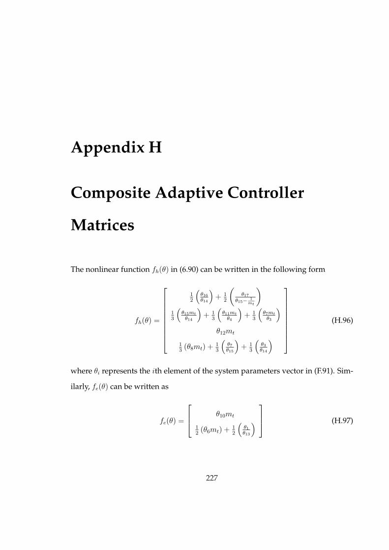
Appendix H
Composite Adaptive Controller
Matrices
The nonlinear function fh(θ) in (6.90) can be written in the following form
fh(θ) =
12
(θ16
θ14
)+ 1
2
(θ17
θ15− 1mt
)
13
(θ15mt
θ14
)+ 1
3
(θ11mt
θ4
)+ 1
3
(θ7mt
θ3
)
θ12mt
13(θ8mt) + 1
3
(θ7
θ15
)+ 1
3
(θ3
θ14
)
(H.96)
where θi represents the ith element of the system parameters vector in (F.91). Sim-
ilarly, fe(θ) can be written as
fe(θ) =
θ10mt
12(θ6mt) + 1
2
(θ1
θ13
)
(H.97)
227
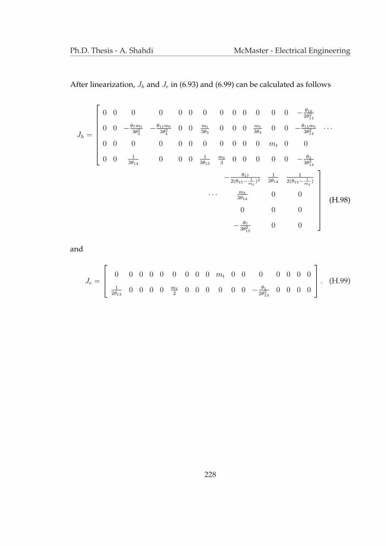
Ph.D. Thesis - A. Shahdi McMaster - Electrical Engineering
After linearization, Jh and Je in (6.93) and (6.99) can be calculated as follows
Jh =
0 0 0 0 0 0 0 0 0 0 0 0 0 − θ16
2θ214
0 0 − θ7mt
3θ23
− θ11mt
3θ24
0 0 mt
3θ30 0 0 mt
3θ40 0 − θ15mt
3θ214
· · ·0 0 0 0 0 0 0 0 0 0 0 mt 0 0
0 0 13θ14
0 0 0 13θ15
mt
30 0 0 0 0 − θ3
3θ214
− θ17
2(θ15− 1mt
)21
2θ14
12(θ15− 1
mt)
· · · mt
3θ140 0
0 0 0
− θ7
3θ215
0 0
(H.98)
and
Je =
0 0 0 0 0 0 0 0 0 mt 0 0 0 0 0 0 0
12θ13
0 0 0 0 mt
20 0 0 0 0 0 − θ1
2θ213
0 0 0 0
. (H.99)
228
Bibliography
[1] S. Sirouspour and A. Shahdi, “Discrete-time linear quadratic gaussian con-
trol for teleoperation under communication time delay,” The International
Journal of Robotics Research, vol. 25, pp. 187–202, 2006.
[2] S. Sirouspour and A. Shahdi, “Model predictive control for transparent tele-
operation under communication time-delay,” IEEE Transactions on Robotics,
vol. 22, no. 6, pp. 1131–1145, 2006.
[3] T. Sheridan, “Telerobotics,” Automatica, vol. 25, no. 4, pp. 487–507, 1989.
[4] C. Melchiorri and A. Eusebi, “Telemanipulation: System aspects and control
issues,” Proceedings of the International Summer School in Modelling and Control
of Mechanisms and Robots, pp. 149–183, 1996.
[5] T. Sheridan, Teletobotics, Automation, and Human Supervisory Control. Cam-
bridge, Massachusetts: The MIT Press, 1992.
[6] P. F. Hokayem. and M. W. Spong, “Bilateral teleoperation: An historical sur-
vey,” Automatica, vol. 42, pp. 2035–2057, 2006.
229

Ph.D. Thesis - A. Shahdi McMaster - Electrical Engineering
[7] S. Salcudean, “Control for teleoperation and haptic interfaces,” Control Prob-
lems in Robotics and Automation LNCIS230, B. Siciliano and K.P. Valavanis (Eds.).
Springer, pp. 51–66, 1998.
[8] T. Sheridan, “Space teleoperation through time delay: review and progno-
sis,” IEEE Transactions on Robotics and Automation, vol. 9, no. 5, pp. 592–606,
1993.
[9] K. Landzettel, B. Brunner, A. Beyer, E. Kramer, and C. Preusche, “Rokviss
verification of advanced teleopresence concepts for future space missions,”
in 7th ESA Workshop on Advances Space Technologies for Robotics and Automa-
tion’ASTRA2002’, Noordwijk, Netherlands, 2002.
[10] G. Hirzinger, G. Grunwald, B. Brunner, and J. Heindl, A sensor-based teler-
obotic system for the space robot experiment ROTEX. Springer, 1993.
[11] M. Oda, “Coordinated control of spacecraft attitude and its manipulator,” in
Proceedings of IEEE International Conference on Robotics and Automation, pp. 732
– 738, 1996.
[12] C. Stoker, D. Barch, B. Hine, and J. Barry, “Antarctic undersea exploration
using a robotic submarine with a telepresence user interface,” IEEE Expert,
vol. 10, no. 6, pp. 14–23, 1995.
[13] D. Kwon, J. Ryu, P. Lee, and S. Hong, “Design of a teleoperation controller for
an underwater manipulator,” in Proceedings of IEEE International Conference
on Robotics and Automation, pp. 3114 – 3119, 2000.
230

Ph.D. Thesis - A. Shahdi McMaster - Electrical Engineering
[14] A. Kwitowski, W. Mayercheck, and A. Brautigam, “Teleoperation for contin-
uous miners and haulage equipment,” IEEE Transactions on Industry Applica-
tions, vol. 28, no. 5, pp. 1118–1125, 1992.
[15] J. Park, K. Kim, H. Lee, and M. Yang, “Robotic contamination cleaning sys-
tem,” in Proceedings of IEEE/RSJ International Conference on Intelligent Robots
and Systems, pp. 1874 – 1879, 2002.
[16] R. Taylor and D. Stoianovici, “Medical robotics in computer-integrated
surgery,” IEEE Transactions on Robotics and Automation, vol. 19, no. 5, pp. 765–
781, 2003.
[17] A. Madhani, G. Niemeyer, and J. Salisbury, “The black falcon: A teleoper-
ated surgical instrument for minimally invasive surgery,” in Proceedings of
IEEE/RSJ International Conference on Intelligent Robots and Systems, pp. 936 –
944, 1998.
[18] D. Lawrence, “Stability and transparency in bilateral teleoperation,” IEEE
Transactions on Robotics and Automation, vol. 9, pp. 624–637, October 1993.
[19] N. Kularatna and D. Dias, Essentials of modern telecommunications systems.
Artech House Publishers, 2004.
[20] A. Rojas, J. Braslavsky, and R. Middleton, “Fundamental limitations in con-
trol over a communication channel,” Automatica, vol. 44, no. 12, pp. 3147–
3151, 2008.
231

Ph.D. Thesis - A. Shahdi McMaster - Electrical Engineering
[21] J. Baillieul and P. Antsaklis, “Control and communication challenges in net-
worked real-time systems,” Proceedings of the IEEE, vol. 95, no. 1, pp. 9–28,
2007.
[22] K. Gu, V. L. Kharitonov, and J. Chen, Stability of Time-Delay Systems. Boston:
Birkhauser, 2003.
[23] J. Slotine, “The robust control of robot manipulators,” The International Jour-
nal of Robotics Research, vol. 4, no. 2, pp. 49–64, 1985.
[24] C. Abdallah, D. Dawson, P. Dorato, and M. Jamshidi, “Survey of robust con-
trol for rigid robots,” IEEE Control Systems Magazine, vol. 11, no. 2, pp. 24–30,
1991.
[25] M. Spong, “On the robust control of robot manipulators,” IEEE Transactions
on Automatic Control, vol. 37, no. 11, pp. 1782–1786, 1992.
[26] H. Sage, M. De Mathelin, and E. Ostertag, “Robust control of robot manipu-
lators: a survey,” International Journal of Control, vol. 72, no. 16, pp. 1498–1522,
1999.
[27] J. Doyle, B. Francis, and A. Tannenbaum, Feedback control theory. Macmillan
New York, 1992.
[28] A. Isidori and W. Kang, “H∞ control via measurement feedback for gener-
alnonlinear systems,” IEEE Transactions on Automatic Control, vol. 40, no. 3,
pp. 466–472, 1995.
232

Ph.D. Thesis - A. Shahdi McMaster - Electrical Engineering
[29] H. Kazerooni, T. Tsay, and K. Hollerbach, “A controller design framework for
telerobotic systems,” IEEE Transactions on Control Systems Technology, vol. 1,
no. 1, pp. 50–62, 1993.
[30] S. Sirouspour, “Modeling and control of cooperative teleoperation systems,”
IEEE Transactions on Robotics, vol. 21, no. 6, pp. 1220–1225, 2005.
[31] J. Yan and S. Salcudean, “Teleoperation controller design using H∞-
optimization with application to motion-scaling,” IEEE Transactions on Con-
trol Systems Technology, vol. 4, no. 3, pp. 244–258, 1996.
[32] G. Leung, B. Francis, and J. Apkarian, “Bilateral controller for teleoperators
with time delay via mu-synthesis,” IEEE Transactions on Robotics and Automa-
tion, vol. 11, no. 1, pp. 105–116, 1995.
[33] O. Sename and A. Fattouh, “Robust H∞ control of bilateral teleoperation sys-
tems under communication time-delay,” Applications of Time Delay Systems.
J. Chiasson and J. J. Loiseau (Eds.). Springer, pp. 99–116, 2007.
[34] W.-H. Zhu and S. Salcudean, “Stability guaranteed teleoperation: an adap-
tive motion/force control approach,” IEEE Transactions on Automatic Control,
vol. 45, no. 11, pp. 1951–1969, 2000.
[35] G. Meinsma and L. Mirkin, “H∞ control of systems with multiple I/O de-
lays via decomposition to adobe problems,” IEEE Transactions on Automatic
Control, vol. 50, no. 2, pp. 199–211, 2005.
233
Ph.D. Thesis - A. Shahdi McMaster - Electrical Engineering
[36] G. Raju, G. Verghese, and T. Sheridan, “Design issues in 2-port network mod-
els of bilateral remote teleoperation,” in Proceedings of IEEE International Con-
ference on Robotics and Automation, pp. 1317–1321, 1989.
[37] B. Hannaford, “A design framework for teleoperators with kinesthetic feed-
back,” IEEE Transactions on Robotics and Automation, vol. 5, no. 4, pp. 426–434,
1989.
[38] Y. Yokokohji and T. Yoshikawa, “Bilateral control of master-slave manipula-
tors for ideal kinesthetic coupling-formulation and experiment,” IEEE Trans-
actions on Robotics and Automation, vol. 10, no. 5, pp. 605–620, 1994.
[39] K. Hastrudi-Zaad and S. Salcudean, “On the use of local force feedback for
transparent teleoperation,” in Proceedings of IEEE International Conference on
Robotics and Automation, vol. 3, 1999.
[40] M. Tavakoli, A. Aziminejad, R. Patel, and M. Moallem, “Discrete-time bilat-
eral teleoperation: modelling and stability analysis,” IET Control Theory &
Applications, vol. 2, no. 6, pp. 496–512, 2008.
[41] A. Abdossalami and S. Sirouspour, “Adaptive Control for Improved Trans-
parency in Haptic Simulations,” IEEE Transactions on Haptics, vol. 2, no. 1,
pp. 2–14, 2009.
[42] K. Hashtrudi-Zaad and S. Salcudean, “Analysis of control architectures for
teleoperation systems with impedance/admittance master and slave manip-
ulators,” The International Journal of Robotics Research, vol. 20, no. 6, pp. 419–
445, 2001.
234
Ph.D. Thesis - A. Shahdi McMaster - Electrical Engineering
[43] S. Haykin, Active network theory. Addison-Wesley Reading, Massachusetts,
USA, 1970.
[44] R. Adams and B. Hannaford, “Stable haptic interaction with virtual environ-
ments,” IEEE Transactions on robotics and Automation, vol. 15, no. 3, pp. 465–
474, 1999.
[45] J.-E. Slotine and W. Li, Applied Nonlinear Control. New Jersey: Prentice-Hall
Inc., 1991.
[46] C. Desoer and M. Vidyasagar, Feedback systems: input-output properties. Aca-
demic Press, Inc. Orlando, FL, USA, 1975.
[47] J. Colgate, “Robust impedance shaping telemanipulation,” IEEE Transactions
on Robotics and Automation, vol. 9, no. 4, pp. 374–384, 1993.
[48] H. Lu and W. Lin, “Robust controller with disturbance rejection for hy-
draulic servo systems,” IEEE Transactions on Industrial Electronics, vol. 39,
no. 1, pp. 157–162, 1993.
[49] N. Niksefat and N. Sepehri, “Robust force controller design for an electro-
hydraulic actuator based on nonlinear model,” in Proceedings of IEEE Inter-
national Conference on Robotics and Automation, pp. 200–206, 1999.
[50] N. Sadegh and R. Horowitz, “Stability and robustness analysis of a class
of adaptive controllers for robotic manipulators,” The International Journal of
Robotics Research, vol. 9, no. 3, pp. 74–92, 1990.
235
Ph.D. Thesis - A. Shahdi McMaster - Electrical Engineering
[51] Z. Hu, S. Salcudean, and P. Loewen, “Robust controller design for teleopera-
tion systems,” in Proceedings of IEEE International Conference on Systems, Man
and Cybernetics, vol. 3, pp. 2127–2132, 1995.
[52] S. Sirouspour and A. Shahdi, “Bilateral teleoperation under communication
time delay using an LQG controller,” in Proceedings of IEEE Conference on
Control Applications, pp. 1257–1262, 2005.
[53] J. Ryu, D. Kwon, and B. Hannaford, “Stable Teleoperation with Time-domain
Passivity Control,” IEEE Transactions on Robotics and Automation, vol. 20,
pp. 365–373, 2004.
[54] D. Lee and P. Li, “Passive bilateral control and tool dynamics rendering for
nonlinear mechanical teleoperators,” IEEE Transactions on Robotics, vol. 21,
no. 5, pp. 936–951, 2005.
[55] R. Kress and J. Jansen, “Automatic tuning for a teleoperated arm controller,”
in Proceedings of IEEE Conference on Decision and Control, pp. 2692–2695, 1992.
[56] K. Hashtrudi-Zaad and S. Salcudean, “Adaptive transparent impedance
reflecting teleoperation,” in Proceedings of IEEE International Conference on
Robotics and Automation, pp. 1369 – 1374, 1996.
[57] M. Shi, G. Tao, H. Liu, and J. H. Downs, “Adaptive control of teleoperation
systems,” in Proceedings of IEEE Conference on Decision and Control, pp. 791 –
796, 1999.
236

Ph.D. Thesis - A. Shahdi McMaster - Electrical Engineering
[58] H. K. Lee, M. H. Shin, and M. J. Chung, “Adaptive control of master-slave
systems for transparent teleoperation,” Journal of Robotic Systems, vol. 15,
pp. 465–475, 1998.
[59] L. Love and W. Book, “Force reflecting teleoperation with adaptive
impedance control,” IEEE Transactions on Systems, Man, and Cybernetics,
vol. 34, no. 1, pp. 159–165, 2004.
[60] K. Ciliz and K. Narendra, “Multiple model based adaptive control of robotic
manipulators,” in Proceedings of IEEE Conference on Decision and Control,
pp. 1305–1310, 1994.
[61] M. Leahy Jr and S. Sablan, “Multiple model-based control of robotic manipu-
lators: an overview,” in Proceedings of IEEE Conference on Decision and Control,
pp. 1976–1977, 1990.
[62] K. Narendra and J. Balakrishnan, “Adaptive control using multiple models,”
IEEE Transactions on Automatic Control, vol. 42, no. 2, pp. 171–187, 1997.
[63] Y. Zhang and J. Jiang, “Integrated active fault-tolerant control using IMM ap-
proach,” IEEE Transactions on Aerospace and Electronic Systems, vol. 37, no. 4,
pp. 1221–1235, 2001.
[64] K. Hashtrudi-Zaad and S. Salcudean, “Transparency in time-delayed sys-
tems and the effect of local force feedback for transparent teleoperation,”
IEEE Transactions on Robotics and Automation, vol. 18, no. 1, pp. 108–114, 2002.
237

Ph.D. Thesis - A. Shahdi McMaster - Electrical Engineering
[65] P. Arcara and C. Melchiorri, “Control schemes for teleoperation with time
delay: A comparative study,” Robotics and Autonomous Systems, vol. 38, no. 1,
pp. 49–64, 2002.
[66] T. Imaida, Y. Yokokohji, T. Doi, M. Oda, and T. Yoshikawa, “Ground-space
bilateral teleoperation of ETS-VII robot arm by direct bilateral coupling un-
der 7-s time delay condition,” IEEE Transactions on Robotics and Automation,
vol. 20, no. 3, pp. 499–511, 2004.
[67] N. Ando, J. Lee, and H. Hashimoto, “A study on influence of time delay in
teleoperation,” in Proceedings of IEEE/ASME International Conference on Ad-
vanced Intelligent Mechatronics, pp. 317–322, 1999.
[68] S. Lee and H. Lee, “Modeling, design, and evaluation of advanced teleoper-
ator controlsystems with short time delay,” IEEE Transactions on Robotics and
Automation, vol. 9, no. 5, pp. 607–623, 1993.
[69] J. Azorin, O. Reinoso, R. Aracil, and M. Ferre, “Generalized control method
by state convergence for teleoperation systems with time delay,” Automatica,
vol. 40, pp. 1575–1582, 2004.
[70] T. Mirfakhrai and S. Payandeh, “A model for time-delays for teleoperation
over the Internet,” in Proceedings of IEEE International Symposium on Compu-
tational Intelligence in Robotics and Automation, pp. 236–241, 2001.
[71] R. Anderson and M. Spong, “Bilateral control of teleoperators with time de-
lay,” IEEE Transactions on Automatic Control, vol. 34, no. 5, pp. 494–501, 1989.
238
Ph.D. Thesis - A. Shahdi McMaster - Electrical Engineering
[72] S. Stramigioli, A. Van der Schaft, B. Maschke, and C. Melchiorri, “Geomet-
ric scattering in robotic telemanipulation,” IEEE Transactions on Robotics and
Automation, vol. 18, no. 4, pp. 588–596, 2002.
[73] G. Niemeyer and J.-J. Slotine, “Stable adpative teleoperation,” IEEE Journal
of Oceanic Engineering, vol. 16, no. 1, pp. 152–162, 1991.
[74] R. Anderson and M. Spong, “Asymptotic stability for force reflecting teleop-
erators with time delay,” The International Journal of Robotics Research, vol. 11,
no. 2, pp. 135–142, 1992.
[75] G. Niemeyer and J.-J. Slotine, “Towards force-reflecting teleoperation over
the internet,” in Proceedings of IEEE International Conference on Robotics and
Automation, pp. 1909–1915, 1998.
[76] J. Ueda and T. Yoshikawa, “Force-reflecting teleoperation with time delay by
signal filtering,” IEEE Transactions on Robotics and Automation, vol. 20, no. 3,
pp. 613–619, 2004.
[77] G. Niemeyer and J. Slotine, “Telemanipulation with time delays,” The Inter-
national Journal of Robotics Research, vol. 11, no. 2, pp. 873–890, 2004.
[78] Y. Yokokohji, T. Imaida, and T. Yoshikawa, “Bilateral control with energy bal-
ance monitoring under time-varying communication delay,” in Proceedings of
IEEE International Conference on Robotics and Automation, pp. 2684–2689, 2000.
[79] Y. Yokokohji, T. Imaida, and T. Yoshikawa, “Bilateral teleoperation under
time-varying communication delay,” in Proceedings of IEEE/RSJ International
Conference on Intelligent Robots and Systems, pp. 1854 – 1859, 1999.
239

Ph.D. Thesis - A. Shahdi McMaster - Electrical Engineering
[80] C. Benedetti, M. Franchini, and P. Fiorini, “Stable tracking in variable time-
delay teleoperation,” in Proceedings of IEEE/RSJ International Conference on
Intelligent Robots and Systems, pp. 2252 – 2257, 2001.
[81] T. Mirfakhrai and S. Payandeh, “A delay prediction approach for teleop-
eration over the internet,” in Proceedings of IEEE International Conference on
Robotics and Automation, pp. 2178 – 2183, 2002.
[82] H. Baier, “Transparency and stability of bilateral kinesthetic teleoperation
with time-delayed communication,” Journal of Intelligent and Robotic Systems:
Theory and Applications, vol. 40, no. 1, pp. 1–22, 2004.
[83] S. Munir and W. Book, “Internet-based teleoperation using wave variables
with prediction,” IEEE/ASME Transactions on Mechatronics, vol. 7, no. 2,
pp. 124–133, 2002.
[84] D. Lee and M. W. Spong, “Passive bilateral teleoperation with constant time
delay,” IEEE Transactions on Robotics, vol. 22, no. 2, pp. 269–281, 2006.
[85] N. Chopra and M. W. Spong, “Adaptive coordination control of bilateral tele-
operators with time delay,” in Proceedings of IEEE Conference on Decision and
Control, pp. 4540–4547, 2004.
[86] N. A. Tanner and G. Niemeyer, “Improving perception in time-delayed teler-
obotics,” The International Journal of Robotics Research, vol. 24, pp. 631–644,
2005.
240
Ph.D. Thesis - A. Shahdi McMaster - Electrical Engineering
[87] H. Ching and W. J. Book, “Internet-based bilateral teleoperation based on
wave variable with adaptive predictor and direct drift control,” Journal of
Dynamic Systems, Measurement, and Control, vol. 128, pp. 86–93, 2006.
[88] A. Bejczy, W. Kim, and S. Venema, “The phantom robot: predictive displays
for teleoperation with time-delay,” in Proceedings of IEEE International Con-
ference on Robotics and Automation, pp. 546–551, 1990.
[89] J. Kikuchi, K. Takeo, and K. Kosuge, “Teleoperation system via computer
network for dynamic environment,” in Proceedings of IEEE International Con-
ference on Robotics and Automation, pp. 3534–3539, 1998.
[90] Z. Ping, K. Tanaka, E. Shimizu, and M. Ito, “A teleoperating system for un-
derwater manipulator with virtual model aid,” in Proceedings of IEEE Inter-
national Conference on Robotics and Automation, pp. 882–886, 2003.
[91] T. Kotoku, “A predictive display with force feedback and its application to
remote manipulation system with transmission time delay,” in Proceedings
of IEEE/RSJ International Conference on Intelligent Robots and Systems, vol. 1,
pp. 239 – 246, 1992.
[92] G. Hirzinger, J. Heindl, and K. Landzettel, “Predictive and knowledge-based
telerobotic control concepts,” in Proceedings of IEEE International Conference on
Robotics and Automation, pp. 1768–1777, 1989.
[93] L. Conway, R. Volz, and M. Walker, “Teleautonomous systems: project-
ing and coordinating intelligentaction at a distance,” IEEE Transactions on
Robotics and Automation, vol. 6, no. 2, pp. 146–158, 1990.
241

Ph.D. Thesis - A. Shahdi McMaster - Electrical Engineering
[94] R. Paul, T. Lindsay, and C. Sayers, “Time delay insensitive teleoperation,” in
Proceedings of IEEE/RSJ International Conference on Intelligent Robots and Sys-
tems, vol. 1, pp. 247 – 254, 1992.
[95] S. Ganjefar, H. Momeni, F. J. Sharifi, and M. H. Beheshti, “Behavior of Smith
predictor in teleoperation systems with modeling and delay time errors,” in
Proceedings of IEEE Conference on Control Applications, pp. 1176 – 1180, 2003.
[96] F. Buzan and T. Sheridan, “A model-based predictive operator aid for tele-
manipulators with time delay,” in Proceedings of IEEE International Conference
on Systems, Man and Cybernetics, pp. 138 – 143, 1989.
[97] A. Bemporad, “Predictive control of teleoperated constrained systems with
unbounded communication delays,” in Proceedings of IEEE Conference on De-
cision and Control, pp. 2133 – 2138, 1998.
[98] A. Casavola, E. Mosca, and M. Sorbara, “Teleoperation of constrained dy-
namical systems over a TCP/IP local network,” in Proceedings of IEEE Inter-
national Conference on Robotics and Automation, pp. 4122–4127, 2004.
[99] P. Prekopiou, S. Tzafestas, and W. Harwin, “Towards variable-time-delays-
robust telemanipulation through masterstate prediction,” in Proceedings
of IEEE/ASME International Conference on Advanced Intelligent Mechatronics,
pp. 305–310, 1999.
[100] K. Gu and S. Niculescu, “Survey on recent results in the stability and control
of time-delay systems,” Journal of Dynamic Systems, Measurement, and Control,
vol. 125, pp. 158–165, 2003.
242

Ph.D. Thesis - A. Shahdi McMaster - Electrical Engineering
[101] J. Richard, “Time-delay systems: an overview of some recent advances and
open problems,” Automatica, vol. 39, pp. 1667–1694, 2003.
[102] K. Watanabe, E. Nobuyama, and A. Kojima, “Recent advances in control of
time delay systems - a tutorial review,” in Proceedings of IEEE Conference on
Decision and Control, pp. 2083 – 2089, 1996.
[103] V. Kharitonov, “Robust stability analysis of time delay systems: a survey,”
Annual Reviews in Control, vol. 23, pp. 185–196, 1999.
[104] A. Olbrot, “Robustness of time-delay systems: a survey,” in Proceedings of
IEEE Conference on Decision and Control, pp. 508 – 514, 1988.
[105] W. Kwon and A. Pearson, “Feedback stabilization of linear systems with de-
layed control,” IEEE Transactions on Automatic Control, vol. 25, no. 2, pp. 266–
269, 1980.
[106] Z. Artstein, “Linear systems with delayed controls: a reduction,” IEEE Trans-
actions on Automatic Control, vol. 27, no. 4, pp. 869–879, 1982.
[107] C. Foias, H. Ozbay, and A. Tannenbaum, Robust control of infinite dimensional
systems:(frequency domain methods). Springer, 1996.
[108] L. Mirkin and G. Tadmor, “H∞ control of system with I/O delay: A review
of some problem-oriented methods,” IMA Journal of Mathematical Control and
Information, vol. 19, pp. 185–199, 2002.
[109] L. Mirkin, “On the extraction of dead-time controllers and estimators from
delay-free parametrizations,” IEEE Transactions on Automatic Control, vol. 48,
no. 4, pp. 543–553, 2003.
243

Ph.D. Thesis - A. Shahdi McMaster - Electrical Engineering
[110] P. Kanjilal, Adaptive prediction and predictive control. Peter Peregrinus Ltd,
1995.
[111] M. Morari and J. H. Lee, “Model predictive control: past, present and fu-
ture,” Computers and Chemical Engineering, vol. 23, no. 4-5, pp. 667–682, 1999.
[112] S. Evesque, A. Annaswamy, S. Niculescu, and A. Dowling, “Adaptive con-
trol of a class of time-delay systems,” Journal of Dynamic Systems, Measure-
ment, and Control, vol. 125, no. 2, pp. 186–193, 2003.
[113] M. T. Nihtila, “Adaptive control of a continuous-time system with time-
varying input delay,” Systems & Control Letters, vol. 12, no. 4, pp. 357–364,
1989.
[114] L. Sciavicco and B. Siciliano, Modeling and Control of Robot Manipulators.
Springer, 2000.
[115] F. Lewis, D. Dawson, and C. Abdallah, Robot manipulator control: theory and
practice. CRC, 2004.
[116] J. Cooke, “Dependence of human arm movements on limb mechanical prop-
erties,” Brain Research, vol. 165, no. 2, pp. 366–369, 1979.
[117] H. Kazerooni and M. Her, “The dynamics and control of a haptic interface
device,” IEEE Transactions on Robotics and Automation, vol. 10, no. 4, pp. 453–
464, 1994.
[118] R. Kelly, R. Carelli, M. Amestegui, and R. Ortega, “On adaptive impedance
control of robot manipulators,” in Proceedings of IEEE International Conference
on Robotics and Automation, pp. 572–577, 1989.
244
Ph.D. Thesis - A. Shahdi McMaster - Electrical Engineering
[119] A. Shahdi and S. Sirouspour, “Multiple model control for teleoperation in
unknown environments,” in Proceedings of IEEE International Conference on
Robotics and Automation, pp. 715–720, 2005.
[120] M. Athans, “The role and use of the stochastic linear-quadratic-Gaussian
problem in control system design,” IEEE Transactions on Automatic Control,
vol. 16, no. 6, pp. 529–552, 1971.
[121] M. Sirouspour and S. Salcudean, “Suppressing operator-induced oscillations
in manual control systems with movable bases,” IEEE Transactions on Control
Systems Technology, vol. 11, no. 4, pp. 448–459, 2003.
[122] C. T. Chen, Linear System Theory and Design. Saunders College Publishing,
1984.
[123] K. Shoarinejad, I. Kanellakopoulos, J. Wolfe, and J. Speyer, “A two-station
decentralized LQG problem with noisy communication,” in Proceedings of
IEEE Conference on Decision and Control, pp. 4953–4958, 1999.
[124] G. C. Goodwin, S. F. Graebe, and M. E. Salgado, Control System Design. Pren-
tice Hall, Inc., 2001.
[125] L. Ni and D. Wang, “A gain-switching control scheme for position-error-
based bilateral teleoperation: contact stability analysis and controller de-
sign,” The International Journal of Robotics Research, vol. 23, no. 3, pp. 255–274,
2004.
245
Ph.D. Thesis - A. Shahdi McMaster - Electrical Engineering
[126] D. L. Mills, “Improved algorithms for synchronizing computer network
clocks,” IEEE/ACM Transactions on Networking (TON), vol. 3, no. 3, pp. 245–
254, 1995.
[127] U. Mackenroth, Robust Control Systems. Springer-Verlag, 2004.
[128] D. Bennett, “What are the advantages of variable stiffness control?,” IEEE
Engineering in Medicine and Biology Magazine, vol. 11, no. 4, pp. 86–87, 1992.
[129] H. Kimura, Chain-Scattering Approach to H∞ Control. Birkhauser, 1996.
[130] C. Riviere, R. Rader, and P. Khosla, “Characteristic of hand motion of eye
surgeons,” in Proceedings of Annual International Conference - IEEE/Engineering
in Medicine and Biology Society, pp. 1690–1693, 1997.
[131] O. Hijab, Introduction to Calculus and Classical Analysis. Springer-Verlag, 1997.
[132] F. Amato, Robust control of linear systems subject to uncertain time-varying pa-
rameters. Springer Verlag, 2006.
[133] K. Zhou, J. Doyle, and K. Glover, Robust and Optimal Control. Prentice-Hall,
1995.
246