Model-based fault diagnosis in rotor systems withself-sensing piezoelectric actuators

Am Fachbereich Maschinenbau

an der Technischen Universität Darmstadt

zur

Erlangung des Grades eines Doktor-Ingenieurs (Dr.-Ing.)

genehmigte

Dissertation

vorgelegt von

Ramakrishnan Ambur Sankaranarayanan, M.Sc.

aus Tirunelveli, Indien

Berichterstatter: Prof. Dr.-Ing. Stephan Rinderknecht

Mitberichterstatter: Prof. Dr.-Ing. Stefan Seelecke

Tag der Einreichung: 25.10.2016

Tag der mündlichen Prüfung: 15.12.2016

Darmstadt 2017

D 17

⸀ხ.- MiLi

Never stop learning.- Auvaiyar

AcknowledgmentI would like to express my gratitude to Prof. Dr.-Ing. S. Rinderknecht for hisguidance with which I could complete my doctoral thesis at Institute for Mecha-tronic Systems in Mechanical Engineering at Technische Universität Darmstadt.I thank Prof. Dr.-Ing. S. Seelecke (Universität des Saarlandes), for accepting tobe the second examiner of my thesis and for his suggestions.

The entire research work was financed by the German Research Foundation(DFG) within their Research Training Group “GRK1344”, with support fromRolls-Royce Deutschland Ltd and Co. KG. I earnestly acknowledge and thankthem here.

My sincere word of thanks goes also to all the colleagues of IMS for their helpthroughout my tenure. I thank Mr. Stefan Heindel, Mr. Fabian Becker and Ms.Xiaonan Zhao for their valuable technical inputs. Apart from scientific advicesMr. Philipp Zech and Mr. Daniel Plöger have also helped me to hone my thesis,for which am very grateful. Special thanks to Mr. Raja Vadamalu for his variedtechnical advises.

I am indebted to my parents for their support, offer namaskarams to Gurus anddedicate this work to the Divine.

Ramakrishnan Ambur Sankaranarayanan,18.01.2017.

iii

AbstractMachines which are developed today are highly automated due to increaseduse of mechatronic systems. Fault detection and isolation are important fea-tures to ensure their reliable operation. This research work aims to achieve anintegrated control and fault detection functionality with minimum number ofcomponents.

Piezomaterials can be used both as sensors and actuators due to their inherentcoupling between electrical and mechanical properties. In this thesis, piezo-electric actuators which are being researched for active vibration control onflexible rotors, are also used as sensors. These self-sensing actuators recon-struct their mechanical deflection from the measured voltage and current sig-nals. The systems under investigation are a numerical aircraft engine modeland its scaled representation in a rotor test bench. Since the actuators aremounted in rotor bearings, their displacement represent the bearing deflectiondirectly.

In this research work, the virtual sensor signals are utilised for model-basedfault diagnosis in rotor systems, with focus on unbalances in rotors. Unbalancemagnitude and phase were estimated in frequency domain using a parame-ter estimation method by least squares optimisation. The robustness of theestimates against signal outliers is improved by method of M-estimators. Iden-tifying the fault location is also explored using the hypothesis of localization offaults.

In simulation, models of both systems (aircraft engine and test bench) wereused to detect unbalance faults. In the former system, the influence of actuatorplacements in fault detection ability is examined. The fault detection methodis also validated at the real test bench, as a first step. The unbalance detectedusing the measured virtual sensor signals is compared against results usingavailable physical sensors. They are found to be in good agreement whichproves sensing capability of the actuators. This sensor-minimal approach couldbe favoured in systems with space constraints.

As a further step, unbalances are detected with self-sensing piezoelectric actua-tors in closed loop with an adaptive algorithm for vibration minimisation. Thiscombined control effort and fault detection as a strategy, is suitable to augmentlevel of automation in a machine.

v

KurzfassungDer Automatisierungsgrad von Maschinen nimmt durch den vermehrten Ein-satz mechatronischer Systeme weiter zu. Fehlererkennung und -Isolation sindwichtig, um ihren zuverlässigen Betrieb zu gewährleisten. Diese Forschungsar-beit strebt nach einer integrierten Regelungs- und Fehlererkennungsstrategiemit einer minimalen Anzahl an Komponenten.

Piezomaterialien können durch die physikalische Kopplung zwischen elek-trischen und mechanischen Eigenschaften sowohl aktorisch als auch sensorischeingesetzt werden. In dieser Arbeit werden Piezoaktoren, die hauptsächlichzur aktiven Schwingungsreduktion an flexiblen Rotoren zum Einsatz kommen,gleichzeitig auch als Sensoren verwendet. Diese selbstsensierenden piezoelek-trischen Aktoren rekonstruieren ihre mechanischen Auslenkungen durch Mes-sung der elektrischen Spannung und des Stroms. Die untersuchten Systemesind Modelle eines Flugtriebwerkes und deren skalierte Ausführung im realenPrüfstand. Da die Aktoren am Rotorlager montiert sind, stellen die rekonstru-ierten Signale die Lagerauslenkung dar.

In dieser Forschungsarbeit werden diese Signale für die modellbasierte Diag-nose der Rotoren eingesetzt. Amplitude und Phase der Unwucht konnten imFrequenzbereich mit parametrischen Ansätzen durch Verwendung der Meth-ode der kleinsten Quadrate ermittelt werden. Zudem wurde die Robustheitder Verfahren gegen Ausreißer durch sogenannte M-Estimators verbessert. DieIdentifikation der Unwuchtlage wurde mit einer Hypothese über die Fehler-lokalisierung untersucht.

In Simulationen wurde die Unwuchterkennung sowohl am Modell des Prüfs-tandes als auch an dem eines Flugtriebwerks untersucht. In letztem Fall wurdeein Einfluss verschiedener Aktorpositionen auf die Güte der Fehlererkennungnachgewiesen. Die Anwendbarkeit der untersuchten Methoden wurde aucham realen Prüfstand gezeigt. Die detektierten Unwuchten aus den rekonstru-ierten Signalen und aus realen Messungen wurden abgeglichen. Sie zeigen einegute Übereinstimmung, welche die Sensierungsfähigkeit der Aktoren nach-weist. Darüber hinaus eignet sich der sensor-minimale Ansatz besonders fürSysteme mit Bauraumeinschränkungen.

Weiterhin wurden auch die Unwuchten mittels selbstsensierender Piezoak-toren mit adaptiven Algorithmen für Schwingungsreduktion im geschlossenen

vii

Regelkreis errechnet. Diese kombinierte Regelung und Fehlerdiagnose ist einweiterer Schritt um den Automatisierungsgrad von Maschinen weiter zu er-höhen.

viii

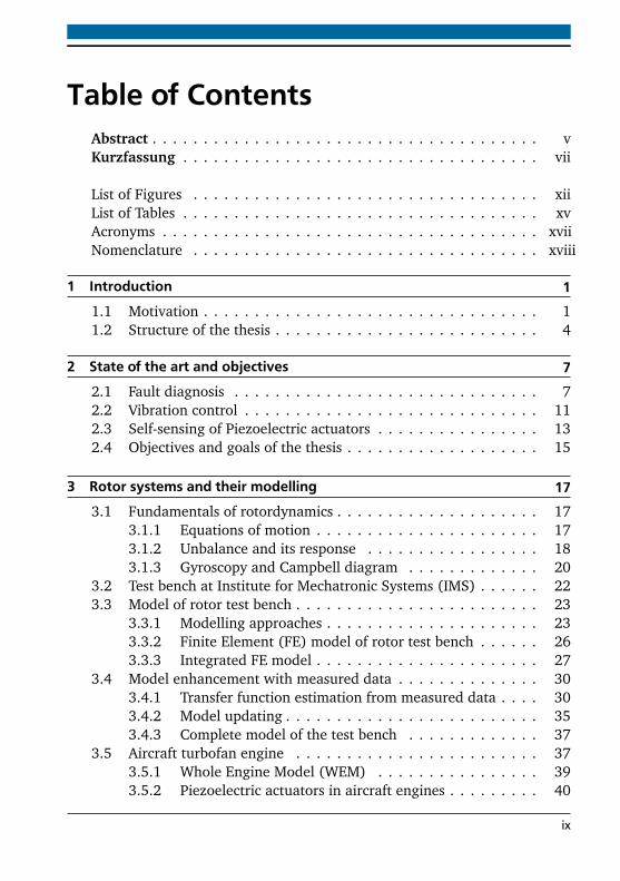
Table of ContentsAbstract . . . . . . . . . . . . . . . . . . . . . . . . . . . . . . . . . . . . . . vKurzfassung . . . . . . . . . . . . . . . . . . . . . . . . . . . . . . . . . . . vii

List of Figures . . . . . . . . . . . . . . . . . . . . . . . . . . . . . . . . . . xiiList of Tables . . . . . . . . . . . . . . . . . . . . . . . . . . . . . . . . . . . xvAcronyms . . . . . . . . . . . . . . . . . . . . . . . . . . . . . . . . . . . . . xviiNomenclature . . . . . . . . . . . . . . . . . . . . . . . . . . . . . . . . . . xviii

1 Introduction 11.1 Motivation . . . . . . . . . . . . . . . . . . . . . . . . . . . . . . . . . 11.2 Structure of the thesis . . . . . . . . . . . . . . . . . . . . . . . . . . 4

2 State of the art and objectives 72.1 Fault diagnosis . . . . . . . . . . . . . . . . . . . . . . . . . . . . . . 72.2 Vibration control . . . . . . . . . . . . . . . . . . . . . . . . . . . . . 112.3 Self-sensing of Piezoelectric actuators . . . . . . . . . . . . . . . . 132.4 Objectives and goals of the thesis . . . . . . . . . . . . . . . . . . . 15

3 Rotor systems and their modelling 173.1 Fundamentals of rotordynamics . . . . . . . . . . . . . . . . . . . . 17

3.1.1 Equations of motion . . . . . . . . . . . . . . . . . . . . . . 173.1.2 Unbalance and its response . . . . . . . . . . . . . . . . . 183.1.3 Gyroscopy and Campbell diagram . . . . . . . . . . . . . 20

3.2 Test bench at Institute for Mechatronic Systems (IMS) . . . . . . 223.3 Model of rotor test bench . . . . . . . . . . . . . . . . . . . . . . . . 23

3.3.1 Modelling approaches . . . . . . . . . . . . . . . . . . . . . 233.3.2 Finite Element (FE) model of rotor test bench . . . . . . 263.3.3 Integrated FE model . . . . . . . . . . . . . . . . . . . . . . 27

3.4 Model enhancement with measured data . . . . . . . . . . . . . . 303.4.1 Transfer function estimation from measured data . . . . 303.4.2 Model updating . . . . . . . . . . . . . . . . . . . . . . . . . 353.4.3 Complete model of the test bench . . . . . . . . . . . . . 37

3.5 Aircraft turbofan engine . . . . . . . . . . . . . . . . . . . . . . . . 373.5.1 Whole Engine Model (WEM) . . . . . . . . . . . . . . . . 393.5.2 Piezoelectric actuators in aircraft engines . . . . . . . . . 40

ix

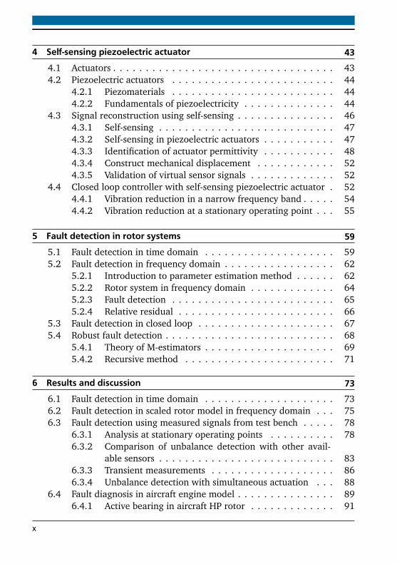
4 Self-sensing piezoelectric actuator 434.1 Actuators . . . . . . . . . . . . . . . . . . . . . . . . . . . . . . . . . . 434.2 Piezoelectric actuators . . . . . . . . . . . . . . . . . . . . . . . . . 44

4.2.1 Piezomaterials . . . . . . . . . . . . . . . . . . . . . . . . . 444.2.2 Fundamentals of piezoelectricity . . . . . . . . . . . . . . 44

4.3 Signal reconstruction using self-sensing . . . . . . . . . . . . . . . 464.3.1 Self-sensing . . . . . . . . . . . . . . . . . . . . . . . . . . . 474.3.2 Self-sensing in piezoelectric actuators . . . . . . . . . . . 474.3.3 Identification of actuator permittivity . . . . . . . . . . . 484.3.4 Construct mechanical displacement . . . . . . . . . . . . 524.3.5 Validation of virtual sensor signals . . . . . . . . . . . . . 52

4.4 Closed loop controller with self-sensing piezoelectric actuator . 524.4.1 Vibration reduction in a narrow frequency band . . . . . 544.4.2 Vibration reduction at a stationary operating point . . . 55

5 Fault detection in rotor systems 595.1 Fault detection in time domain . . . . . . . . . . . . . . . . . . . . 595.2 Fault detection in frequency domain . . . . . . . . . . . . . . . . . 62

5.2.1 Introduction to parameter estimation method . . . . . . 625.2.2 Rotor system in frequency domain . . . . . . . . . . . . . 645.2.3 Fault detection . . . . . . . . . . . . . . . . . . . . . . . . . 655.2.4 Relative residual . . . . . . . . . . . . . . . . . . . . . . . . 66

5.3 Fault detection in closed loop . . . . . . . . . . . . . . . . . . . . . 675.4 Robust fault detection . . . . . . . . . . . . . . . . . . . . . . . . . . 68

5.4.1 Theory of M-estimators . . . . . . . . . . . . . . . . . . . . 695.4.2 Recursive method . . . . . . . . . . . . . . . . . . . . . . . 71

6 Results and discussion 736.1 Fault detection in time domain . . . . . . . . . . . . . . . . . . . . 736.2 Fault detection in scaled rotor model in frequency domain . . . 756.3 Fault detection using measured signals from test bench . . . . . 78

6.3.1 Analysis at stationary operating points . . . . . . . . . . 786.3.2 Comparison of unbalance detection with other avail-

able sensors . . . . . . . . . . . . . . . . . . . . . . . . . . . 836.3.3 Transient measurements . . . . . . . . . . . . . . . . . . . 866.3.4 Unbalance detection with simultaneous actuation . . . 88

6.4 Fault diagnosis in aircraft engine model . . . . . . . . . . . . . . . 896.4.1 Active bearing in aircraft HP rotor . . . . . . . . . . . . . 91

x

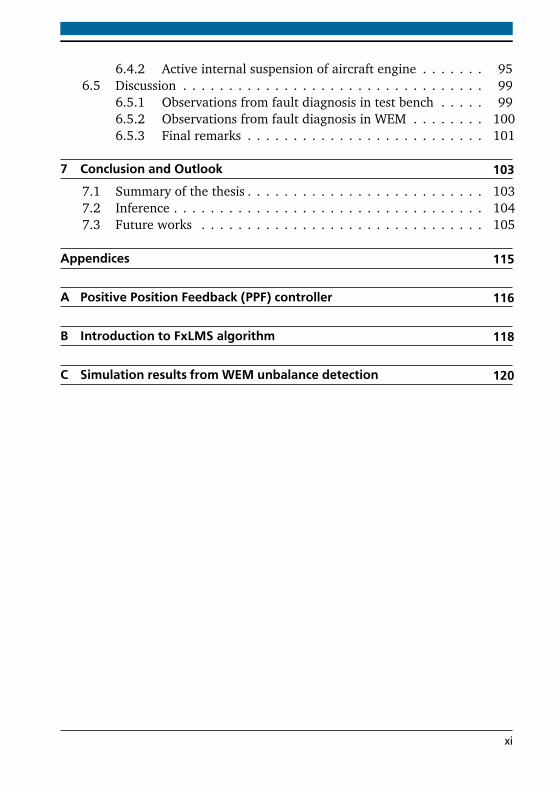
6.4.2 Active internal suspension of aircraft engine . . . . . . . 956.5 Discussion . . . . . . . . . . . . . . . . . . . . . . . . . . . . . . . . . 99

6.5.1 Observations from fault diagnosis in test bench . . . . . 996.5.2 Observations from fault diagnosis in WEM . . . . . . . . 1006.5.3 Final remarks . . . . . . . . . . . . . . . . . . . . . . . . . . 101

7 Conclusion and Outlook 1037.1 Summary of the thesis . . . . . . . . . . . . . . . . . . . . . . . . . . 1037.2 Inference . . . . . . . . . . . . . . . . . . . . . . . . . . . . . . . . . . 1047.3 Future works . . . . . . . . . . . . . . . . . . . . . . . . . . . . . . . 105

Appendices 115

A Positive Position Feedback (PPF) controller 116

B Introduction to FxLMS algorithm 118

C Simulation results from WEM unbalance detection 120

xi

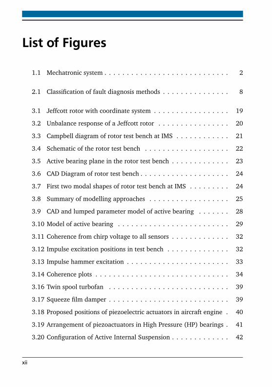
List of Figures

1.1 Mechatronic system . . . . . . . . . . . . . . . . . . . . . . . . . . . . 2

2.1 Classification of fault diagnosis methods . . . . . . . . . . . . . . . 8

3.1 Jeffcott rotor with coordinate system . . . . . . . . . . . . . . . . . 19

3.2 Unbalance response of a Jeffcott rotor . . . . . . . . . . . . . . . . 20

3.3 Campbell diagram of rotor test bench at IMS . . . . . . . . . . . . 21

3.4 Schematic of the rotor test bench . . . . . . . . . . . . . . . . . . . 22

3.5 Active bearing plane in the rotor test bench . . . . . . . . . . . . . 23

3.6 CAD Diagram of rotor test bench . . . . . . . . . . . . . . . . . . . . 24

3.7 First two modal shapes of rotor test bench at IMS . . . . . . . . . 24

3.8 Summary of modelling approaches . . . . . . . . . . . . . . . . . . 25

3.9 CAD and lumped parameter model of active bearing . . . . . . . 28

3.10 Model of active bearing . . . . . . . . . . . . . . . . . . . . . . . . . 29

3.11 Coherence from chirp voltage to all sensors . . . . . . . . . . . . . 32

3.12 Impulse excitation positions in test bench . . . . . . . . . . . . . . 32

3.13 Impulse hammer excitation . . . . . . . . . . . . . . . . . . . . . . . 33

3.14 Coherence plots . . . . . . . . . . . . . . . . . . . . . . . . . . . . . . 34

3.16 Twin spool turbofan . . . . . . . . . . . . . . . . . . . . . . . . . . . 39

3.17 Squeeze film damper . . . . . . . . . . . . . . . . . . . . . . . . . . . 39

3.18 Proposed positions of piezoelectric actuators in aircraft engine . 40

3.19 Arrangement of piezoactuators in High Pressure (HP) bearings . 41

3.20 Configuration of Active Internal Suspension . . . . . . . . . . . . . 42

xii

4.1 Functional diagram of a general actuator . . . . . . . . . . . . . . 43

4.2 Piezoelectric actuators . . . . . . . . . . . . . . . . . . . . . . . . . . 44

4.3 Axes convention in piezo materials . . . . . . . . . . . . . . . . . . 46

4.4 Functional diagram of a general self-sensing actuator . . . . . . . 47

4.5 Sensor construction process of the actuator . . . . . . . . . . . . . 48

4.6 FRF of actuators in parallel planes (Actuator to Strain gauge) . . 49

4.7 Hysteresis estimated from piezoelectric actuators . . . . . . . . . 51

4.8 Magnitude response of band-pass filter . . . . . . . . . . . . . . . . 51

4.9 Compare displacement signals in time domain . . . . . . . . . . . 53

4.10 Comparison of Frequency Response Function (FRF) between thevoltage and displacement signal . . . . . . . . . . . . . . . . . . . . 53

4.11 Block diagram of self-sensing in a closed loop . . . . . . . . . . . . 54

4.12 Performance of Positive Position Feedback (PPF) Controller . . . 56

4.13 Performance of Filtered x-Least mean squares (FxLMS) algorithm 58

5.1 Modified equivalent load minimisation method for unbalancedetection in time domain . . . . . . . . . . . . . . . . . . . . . . . . 61

5.2 Parameter estimation by output-error method . . . . . . . . . . . 62

5.3 Fault detection in a closed loop system . . . . . . . . . . . . . . . . 67

6.1 Unbalance rings . . . . . . . . . . . . . . . . . . . . . . . . . . . . . . 75

6.2 Relative residuals from simulations with test bench model . . . . 77

6.3 Relative deviation in magnitude of strain signals . . . . . . . . . . 81

6.4 FRF and Coherence of Impulse in Ring 4 to Strain . . . . . . . . . 82

6.5 Relative residual with measurements from stationary points . . . 83

6.6 Relative residual with transient measurements . . . . . . . . . . . 87

6.7 Relative residual with simultaneous actuation and sensing . . . . 89

xiii

6.8 Relative residual plot from quasi-static run in active bearings(Piezos and SFD in series) . . . . . . . . . . . . . . . . . . . . . . . . 93

6.9 Relative residual plot from quasi-static run in active bearings(Piezos and SFD in parallel) . . . . . . . . . . . . . . . . . . . . . . 94

6.10 Relative residual plot from quasi-static run in active internal sus-pension when all four actuators are considered . . . . . . . . . . . 96

6.11 Relative residual - Active Internal suspension special cases . . . . 98

A.1 Block diagram of rotorsystem with PPF . . . . . . . . . . . . . . . . 117

B.1 Block diagram of a FxLMS algorithm . . . . . . . . . . . . . . . . . 118

C.1 Relative residual of unbalance detection at all stages - Activebearing (Piezo,SFD series) . . . . . . . . . . . . . . . . . . . . . . . 122

C.2 Relative residual of unbalance detection at all stages - Activebearing (Piezo,SFD parallel) . . . . . . . . . . . . . . . . . . . . . . 125

C.3 Relative residual of unbalance detection at all stages - Activeinternal suspension . . . . . . . . . . . . . . . . . . . . . . . . . . . . 128

xiv

List of Tables

3.1 Matrices in equations of motion . . . . . . . . . . . . . . . . . . . . 17

3.2 Parameters in active bearing model . . . . . . . . . . . . . . . . . . 28

3.3 Parameters estimated by optimisation algorithm . . . . . . . . . . 35

4.1 Variables and Parameters in piezoelectric equation . . . . . . . . . 45

6.1 Unbalance detected from time domain FDI . . . . . . . . . . . . . 74

6.2 Detected unbalances from Test bench (simulation) . . . . . . . . 76

6.3 Unbalance test cases . . . . . . . . . . . . . . . . . . . . . . . . . . . 79

6.4 Unbalance identified from stationary operating points . . . . . . 80

6.5 Comparison of unbalance magnitude identified from differentsensors . . . . . . . . . . . . . . . . . . . . . . . . . . . . . . . . . . . 84

6.6 Comparison of unbalance phase identified from different sensors 85

6.7 Unbalance identified from operating points in transient run . . . 87

6.8 Unbalance identified from simultaneous actuation and sensing . 88

6.9 Detected unbalances from WEM (Active bearing - Piezo and SFDin series) . . . . . . . . . . . . . . . . . . . . . . . . . . . . . . . . . . 91

6.10 Detected unbalances from WEM (Active bearing - Piezo and SFDin parallel) . . . . . . . . . . . . . . . . . . . . . . . . . . . . . . . . . 95

6.11 Detected unbalances from WEM (Active internal suspension - Allfour actuators) . . . . . . . . . . . . . . . . . . . . . . . . . . . . . . . 97

6.12 Detected unbalances from WEM using robust estimators (Activeinternal suspension) . . . . . . . . . . . . . . . . . . . . . . . . . . . 98

C.1 Detected unbalances from WEM (Active bearing - Piezo and SFDin series) - without any outlier . . . . . . . . . . . . . . . . . . . . . 120

xv

C.2 Detected unbalances from WEM (Active bearing - Piezo and SFDin series) - with outliers . . . . . . . . . . . . . . . . . . . . . . . . . 121

C.3 Detected unbalances from WEM (Active bearing - Piezo and SFDin series) - with robust estimators . . . . . . . . . . . . . . . . . . . 121

C.4 Detected unbalances from WEM (Active bearing - Piezo and SFDin parallel) - without any outlier . . . . . . . . . . . . . . . . . . . . 123

C.5 Detected unbalances from WEM (Active bearing - Piezo and SFDin parallel) - with outliers . . . . . . . . . . . . . . . . . . . . . . . . 123

C.6 Detected unbalances from WEM (Active bearing - Piezo and SFDin parallel) - with robust estimators . . . . . . . . . . . . . . . . . . 124

C.7 Detected unbalances from WEM (Active internal suspension) -without any outlier . . . . . . . . . . . . . . . . . . . . . . . . . . . . 126

C.8 Detected unbalances from WEM (Active internal suspension) -with outliers . . . . . . . . . . . . . . . . . . . . . . . . . . . . . . . . 126

C.9 Detected unbalances from WEM (Active internal suspension) -with robust estimators . . . . . . . . . . . . . . . . . . . . . . . . . . 127

xvi

AcronymsCAD Computer Aided Design.CMS Component Mode Synthesis.DOF Degrees of freedom.FDI Fault detection and Isolation.FE Finite Element.FIR Finite Impulse Response.FRF Frequency Response Function.FTC Fault tolerant control.FxLMS Filtered x-Least mean squares.GA Genetic Algorithm.HP High Pressure.IMS Institute for mechatronic systemsLMS Least Mean Squares.LP Low Pressure.LPV Linear Parameter Variant.LQG Linear Quadratic Gaussian.MIMO Multi Input Multi Output.PPF Positive Position Feedback.RC Resonant controller.RLS Recursive Least Squares.SFD Squeeze Film Damper.SISO Single Input Single Output.SVD Singular Value Decomposition.WEM Whole Engine Model.WLS Weighted least squares.

xvii

Nomenclature

Alphabetical symbols

A Cross section areaa Weighing factorC Boolean matrixCx y Coherence between signal y and xds f d Damping factor of SFDd PiezoconstantD Damping matrixD Electrical flux densityE Electrical field strengthe ErrorF Force vectorFU(s) Force due to actuation voltageG Transfer functionG Gyroscopic matrixg Gain of PPF controllerH Estimated transfer functionIp Polar moment of inertiaIt Transversal moment of inertiaI Current in Piezoelectric actuatori Imaginary numberK Stiffness matrixKd yn Dynamic Stiffness matrixk Time discrete samplekd Time delaykact Stiffness of piezo-actuatorl lengthM Mass matrixn Number of stacks of piezoceramicq Charge in a piezo materialq Generalized displacement vectorR Reduced inverted dynamic stiffness matrixS Mechanical strain

xviii

Spx Cross spectral density from signal p to xsE Elasticity modules Laplace operatorT Transformation matrixt Time vectorU Voltage of Piezoelectric actuatorV Optimisation functionW Weighing matrixXm Measured vibrationsx Real value of xx Displacement vectorx Velocity vectorx Acceleration vectoryp Particular solution of lateral displacementz Measured signal with unbalanced rotorz0 Measured reference signalzp Particular solution of lateral displacementZ Circulatory matrix

Greek and Latin symbols

α Proportionality constantβ Integration constantγy Integration constantγ Forgetting factor∆l Extension of piezo materialδ Residualδr Relative Residualδz Relative deviation between measured signalsε Eccentricityεσ Electrical permittivityεS Electrical permittivityΘ Parameter vectorκ Weighing factorµ Step size of FxLMS algorithmξ f Damping in PPF controllerρ Optimisation functionσ Mechanical stress

xix

Φ Eigen vector matrixφ Phase of unbalanceΨ Data vectorΩ Rotational speedω Eigen frequencyω f Target frequency

xx

1 Introduction

1.1 Motivation

Rotating machinery comprise a huge class of mechanical structures, which canbe sighted in almost every walk of human life. They exist in form of electrome-chanical machines such as electric motors and generators, turbomachines suchas pumps and turbines. In all of them vibration is an inevitable and undesiredphenomenon. Vibrations could lead to failure of the machine or in precisionequipments affect its operation. They also cause discomfort to the users forexample the passengers in a vehicle.

The most common sources of vibration in machinery are related to inertia ofmoving parts in the machine. According to Newtons law, a force is needed toaccelerate the mass which in return is transmitted to the frame of the machine.In a stationary operating point these forces in rotating machinery are periodicand hence periodic displacements are observed as vibration. There are manydifferent techniques practised to minimise vibration related issues due to forcedexcitation [1].

1. Introduce damping in the system

2. Include a vibration dynamic absorber

3. Tune the natural frequency of the system away from operating range

4. Identify and reduce the excitation source

5. Isolate the source and the receiver

At the outset, there is much research being done to damp the vibrations bothby passive and active methods. In passive methods, machine elements withfluids are developed which dissipate the vibration energy, a shock absorber inautomobiles is classical example. Active methods might require an additionalenergy input to damp the vibrations in some cases. One of the examples is a

1

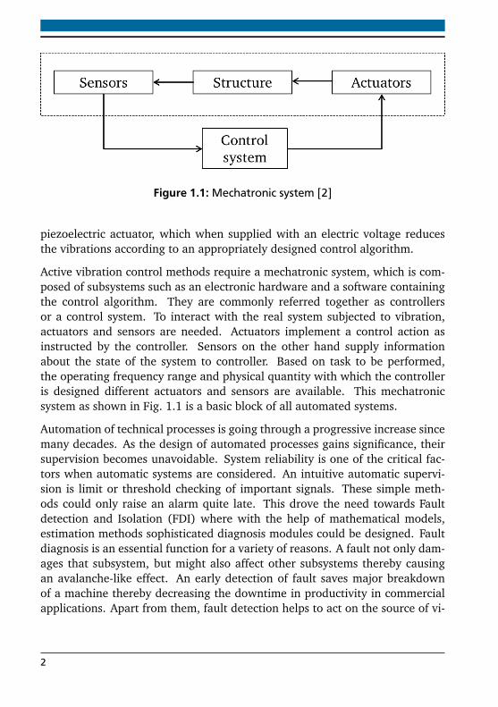
Figure 1.1: Mechatronic system [2]

piezoelectric actuator, which when supplied with an electric voltage reducesthe vibrations according to an appropriately designed control algorithm.

Active vibration control methods require a mechatronic system, which is com-posed of subsystems such as an electronic hardware and a software containingthe control algorithm. They are commonly referred together as controllersor a control system. To interact with the real system subjected to vibration,actuators and sensors are needed. Actuators implement a control action asinstructed by the controller. Sensors on the other hand supply informationabout the state of the system to controller. Based on task to be performed,the operating frequency range and physical quantity with which the controlleris designed different actuators and sensors are available. This mechatronicsystem as shown in Fig. 1.1 is a basic block of all automated systems.

Automation of technical processes is going through a progressive increase sincemany decades. As the design of automated processes gains significance, theirsupervision becomes unavoidable. System reliability is one of the critical fac-tors when automatic systems are considered. An intuitive automatic supervi-sion is limit or threshold checking of important signals. These simple meth-ods could only raise an alarm quite late. This drove the need towards Faultdetection and Isolation (FDI) where with the help of mathematical models,estimation methods sophisticated diagnosis modules could be designed. Faultdiagnosis is an essential function for a variety of reasons. A fault not only dam-ages that subsystem, but might also affect other subsystems thereby causingan avalanche-like effect. An early detection of fault saves major breakdownof a machine thereby decreasing the downtime in productivity in commercialapplications. Apart from them, fault detection helps to act on the source of vi-

2

bration, as mentioned in fourth action in the list above. Other indirect benefitsare to prevent any degradation of efficiency and to protect users.

As mentioned earlier, sensors inform the controllers regarding the state of therotor. This means that the information from the sensor is inevitable even torecognise a defective state. To supply information regarding vibrations in asystem, either accelerometers, velocity transducers or displacement sensorsare included. One among them is selected based on the frequency rangeof operation and whether they are mounted on bearing block or near shaft.These sensors along with their necessary cabling increase the cost. Also not alllocations which are important could be accessible to mount sensors and to laytheir cables. This necessitates a sensor minimal system, where the aim is touse as less sensors as possible and to extract sufficient information. A furtherextension could be to extract information without any dedicated sensors, butwith self-sensing.

In this thesis the second approach is attempted using piezoelectric actuators.Because piezo materials have an inherent electro-mechanical coupling, theyare used in sensors as well as actuators. This provides an opportunity to useonly one component for both actuation and sensing. Hence high voltage piezo-electric actuators which are being developed for vibration control are used alsoas sensors for fault diagnosis.

The thesis focuses on faults occurring in rotor systems. The main faults whichappear in them are

• unbalance,

• misalignment,

• rub or erosion,

• cracks in shafts or blades,

• bearing failures and

• fluid-induced instability

A combination of faults or one leading to another is also possible. Unbalanceis the main reason for majority of faults occurring in rotor systems. It occurs inrotors due to manufacturing defects, where additional mass could be presentor removed at any particular location along the shaft. During commissioningthey have to be compensated by balancing them, by placing counter-balancing

3

masses at pre-decided locations. The rotor is then brought to acceptable vi-bration limits [3]. Even after balancing, during an operation there could beremoval of mass due to erosion of the rotating parts with static parts leadingto unbalanced condition. Hence there is a need for condition monitoring atregular intervals.

There are two rotor systems being investigated in this research work for un-balance faults. The first system is an turbofan aircraft engine. In a simulationmodel of the engine, only the HP rotor is focussed. Piezoelectric actuators arealready being investigated for their potential to reduce vibration in them. Inthe present research work, three actuator positions are analysed for their ef-fectiveness in detecting faults, if sensor signals could be extracted from theseactuators.

The second rotor system is a real test bench built in IMS. In this rotor testbench, a shaft downscaled from a Turbopropeller engine rotor is mounted.Piezoelectric actuators were mounted at their bearings with an aim to activelycontrol vibrations [4]. Using self-sensing techniques sensor signals are recon-structed from the actuator signals, thereby using them as self-sensing actuators.The mechanical displacement of actuator reconstructed from its electrical sig-nals represent the bearing deflection. With the help of this deflection unbalancefaults are detected. The effectiveness of the fault detection method is examinedwith model and the real test bench.

1.2 Structure of the thesis

After introduction, the thesis continues with a literature review in Chapter 2.Detailed review regarding the fault diagnosis in rotor systems and differentapproaches in the past has been presented. A brief summary of active vibra-tion control and effectiveness of piezoelectric actuators in rotor systems is alsodescribed. Further, previous attempts of self-sensing in piezoelectric actuatorsand different approaches are mentioned. Briefly, fault diagnosis in a closedcontrol loop and its basic difference from a fault tolerant control system is ex-plained. Out of the literature survey, the gaps in research are identified andthe goals for this thesis are extracted and presented towards the end of thechapter.

In Chapter 3, fundamentals of rotor systems are introduced. The systems whichare used for this thesis are presented. The first is a test bench available at the in-stitute. Its mathematical model is also described along with a brief description

4

on grey-box modelling approach using modal testing techniques. The secondsystem is a high pressure rotor system of an aircraft engine. Its finite elementmodel was designed by its manufacturer, in which piezoelectric actuators wereincluded later on at specific locations.

Chapter 4 describes a piezoelectric actuator and introduces self-sensing. Thetwo step procedure of self-sensing for the actuator mounted in the rotor systemhas been explained. Further the reconstructed virtual signals are comparedwith real sensor signals. The virtual signals were also used in a closed loopfor active vibration control, to prove that the actuator could simultaneouslyactuate and sense.

Fault detection is first introduced in Chapter 5. Before the process of fault es-timation is begun, a mathematical introduction on parameter estimation tech-nique is presented. Further the unbalance detection in time and frequencydomain are explained, though only the latter is analysed further in the thesis.Fault location could be possibly determined by a scalar called relative residual.An important take-off from this thesis is the unbalance detection in a closedloop which is explained thereafter. Finally an alternative to the common leastsquares approach is presented for a robust parameter detection.

The results are presented in Chapter 6. At first the observations from simu-lations using the aircraft model and test bench model are presented. Laterthe unbalance detection applied on signals measured from the test bench areshown. The results are then discussed.

Finally Chapter 7 concludes the thesis and presents scope for future work.

5

2 State of the art and objectivesLiterature survey in this chapter is presented in two broad sections. The firstsection discusses about fault diagnosis in rotor systems. This is then followedby the section on works associated with vibration control, some of them wherepiezoelectric actuators are used. After that research towards self-sensing inpiezoelectric actuators are presented. At the end, challenges faced in this re-search are derived from them and the objectives of the thesis are presented.

2.1 Fault diagnosis

Fault diagnosis is a combination of three tasks as listed below

1. Fault detection - Determine the occurrence of faults by triggering alarmsignals

2. Fault isolation - Classification of faults

3. Fault analysis or identification - Determining the magnitude, type andcause of fault

Faults in engineering systems are diagnosed by a broad spectrum of methods.Their classification has been presented in Fig. 2.1 by [5]. In the first schemecalled hardware redundancy, additional identical hardware components areincluded in the system. Faults are detected if system output differs from theadditional hardware’s output. Plausibility tests are based on comparison withbasic physical laws. The last scheme is to diagnose faults by signal processingmethods, which are advantageous only in steady-state processes. They cannotbe used for processes which have a wide operating range due to variation ofinput signals. Because this thesis strives to reduce the components in the sys-tem, software redundancy is attempted instead of hardware redundancy. Withthis scheme, an analytical model of the system is created and compared withthe system for any difference in behaviour.

Conventionally model-based fault diagnosis are performed by parity equationsor parameter estimation method or their combination. The former is applicable

7

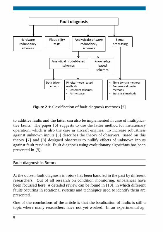
Figure 2.1: Classification of fault diagnosis methods [5]

to additive faults and the latter can also be implemented in case of multiplica-tive faults. The paper [6] suggests to use the latter method for instationaryoperation, which is also the case in aircraft engines. To increase robustnessagainst unknown inputs [5] describes the theory of observers. Based on thistheory [7] and [8] designed observers to nullify effects of unknown inputsagainst fault residuals. Fault diagnosis using evolutionary algorithms has beenpresented in [9].

Fault diagnosis in Rotors

At the outset, fault diagnosis in rotors has been handled in the past by differentresearchers. Out of all research on condition monitoring, unbalances havebeen focussed here. A detailed review can be found in [10], in which differentfaults occuring in rotational systems and techniques used to identify them arepresented.

One of the conclusions of the article is that the localisation of faults is still atopic where many researchers have not yet worked. In an experimental ap-

8

proach in [11] optical sensors were used to localise unbalances in inductionmotors. But it is not practical in large turbines where many rows of bladesare mounted. Analytically, Hilbert-Huang transforms were used in [12] to lo-calise faults in a dual disk setup, but still a comprehensive validation for thepresented theory is lacking. A data-driven technique has been developed by[13] in which operating deflection shapes have been measured in a machinefault simulator. However it is not suitable for large machines and also due tonumber of sensors used.

Unbalances in rotor systems are detected by observer based methods in [14]following the work by [15]. Another precursor is use of unknown input ob-server methods by [16]. In [17], a single transducer was used to balance rotorin different planes.

One of the earlier works to detect unbalance based on a model using leastsquares approach is by [18] and [19], where the measured signals from thesystem were compared to a reference model. Here the authors used the modalexpansion method, to extrapolate the vibration signals at any other degree offreedom, when sensors could not be positioned at all important locations. Thismethod is one of the first pointers towards a sensor minimal fault detection.However a very accurate model is presumed, and the technique was demon-strated only in a Jeffcott rotor. The theory was extended by [20], where themodal expansion was applied to the signals of the model also, to overcomemathematical problems. Again here the theory was proven only in a singlemass rotor where the position of unbalance was known a-priori.

These problems are overcome by the frequency domain parameter estimationmethod presented by [21] and [22], where multiple faults could be deter-mined. This theory has been used in the present thesis for fault detection.However this method considers faults investigated without any active vibra-tion controller implemented. Hence the theory should be extended to consideractuation forces from piezoelectric actuators.

Modeling efforts for fault detection

In another detailed review paper by [23], a concise list of modeling effortswere given and their use for fault diagnosis is given. It can be seen here thatfor unbalance fault detection, finite element method for a mathematical modelof rotor has been the desired choice by different researchers. To update the

9

speed dependency of models of rotor systems [24] presents a method withwhich a second parallel model complements the output from a neural networkmodel. Similar procedure was also adopted in [25].

However a complete mathematical model is still not available for conditionmonitoring in many cases. Hence using different estimation methods, the par-tially constructed model can be updated. Most of the model updating meth-ods use optimisation routines to minimise the error the between the measuredtransfer function and model. Here ill-conditioned problems are a challenge,which should be solved by Singular Value Decomposition (SVD) method. Anearly reference to model updating is given in [26]. One of the conclusion is tomatch atleast one-third of all the eigen frequencies in the operating range foraccurate design purpose. The paper [27] shows a method to calibrate a modelin which the rotor is mounted on anisotropic bearings. A recent compilation in[28] describes different direct and iterative methods for finite element modelupdating.

In all methods for model updating, modal analysis plays an important role.One of earliest references towards it can be found in [29]. More can be under-stood from [30] where a mathematical background to extract modal model inrotating structures has been presented.

Previous works at IMS

At IMS, there were many research works done on fault diagnosis in rotors. Inone of the first works by [31], magnetic bearings were implemented for themodel-based fault diagnosis in a centrifugal pump. Here signal- and model-based FDI are performed. The signal based fault detection is based on com-puting the changes in modal parameters such as eigen frequencies and modaldamping when faults occur. In model-based FDI, the transfer function betweenthe model and process are compared to detect faults. The magnetic bearingsare used to excite the system with signals of known frequencies to reproducethe transfer function.

In another work by [32], the previous setup of a centrifugal pump with mag-netic bearings was investigated further. Here using parameter estimation meth-ods the modal parameters were estimated. However better results were ob-tained using a transfer function based approach. Using parity equations basedapproach, two variants to calculate residuals were researched. One uses filters

10

to weigh the residues and another method uses Kalman filters. Different typesof errors were diagnosed with the help of a bank of models.

The first implementation of piezoelectric actuators for active bearings was doneby [33]. A Jeffcott rotor with a single rotating disc in the centre was mountedbetween a passive and an active bearing. Sensor and actuator faults werediagnosed with the help of bank of observers. Unbalance as a process faultwas diagnosed with the help of force and displacement sensors available atthe setup. Another novel method is the implementation of FxLMS algorithm todetermine the unbalance parameters using its filter coefficients. In the researchwork, the idea towards sensor minimality was initiated by implementing anobserver instead of force sensors.

The work of [34] describes a method implementing the conventional par-ity equations as unknown input observers for fault detection. Hereby thegyroscopy, model uncertainties are classified as unknown inputs whose dis-tribution was estimated and their effects nullified during the fault diagnosisprocedure.

The different studies mentioned here present the fault diagnosis in rotationalsystems with active bearings. However the active magnetic bearing or thepiezoelectric actuator was used only as an actuating device, but not for simul-taneous sensing. Also parameter estimation techniques in frequency domainwere not investigated in a rotor with significant gyroscopic terms.

2.2 Vibration control

Out of different measures to reduce vibrations in Section 1.1, isolating thevibration source and the receiver is another important focus of various re-searchers. This is necessary to interrupt the vibration transmission path, sothat other subsystems or the end user remain unaffected. In this section, vi-brations arising out of unbalances in rotor systems are focussed and differentworks to control them are reviewed.

Balancing in aircraft engines

In a turbofan aircraft engine, the fan visible from outside is mounted on theLow Pressure (LP) rotor. So on account of an unbalance after the complete

11

engine assembly, counter-balancing masses can still be screwed to the low-pressure rotor at the nose of the turbo-fan. On the other hand, HP rotor of theengine is not accessible after the complete engine has been built [35]. Hencemost part of the balancing should be done during the assembly itself.

The paper [36] describes in detail the vibration health monitoring of the engineboth on-board and on-ground. In on-board diagnosis, the analysing softwaremonitors the vibration signals from different transducers and categorises basedon the flight maneuver, static or transient conditions and also the ambient at-mospheric conditions. The on-ground diagnosis analyses the trend of vibrationsignals, uses sophisticated methods based on artificial intelligence for diagnosisof vibration events. Out of the different faults which could be diagnosed thisway, important are the out-of-balance due to normal deterioration, ice buildupin LP compressor blades, excess out-of-balance due to bird strike or blade loss.Another paper presented by [37], lists the different corrective actions done inan aircraft engine to avoid or mitigate the faults. The unbalance vibrationscould be damped by Squeeze Film Damper (SFD), or can be mitigated by ad-justing the balancing masses between the compressor and the turbine in thesame circumferential position.

However these and the other corrective actions mentioned are to be done eitherin the design phase or in the test phase, not during the operation of the engine.So either balancing or vibration control measures should be implemented asand when it occurs.

Passive vibration control

In order to damp vibrations, many machine elements were constructed withfluids to dissipate vibrations. One of them is a vibration absorber [38]. Alsosolid blocks of rubber or fluid mounts or SFD were implemented [39]. Thedisadvantage of these elements are their limited working range. However laterthey were extended to semi-active components such as hybrid SFD [40] oradaptive fluid mounts [41].

Their disadvantages are mainly the non-linear behaviour of fluid elements,which poses difficulties in their analysis. Moreover an oil supply is also needed.With a drive towards More Electric Aircraft [42], it is desired to replace hy-draulic or pneumatic components with electrical components. They ensure anapproximately linear and more importantly a predictable functioning.

12

Active vibration control

For a wider operating range and also for better control over system dynamics,active components are researched. One of earliest works include [43] and [44].Since then active bearings as an effective means for damping rotor vibrationshave been exhaustively researched.

The motivation for this research is due to the limitations posed by passivedamping elements such as SFD. In a scaled low pressure turbine test setup,[4] investigated the efficacy of a PDT1 controller and a observer based LQGcontroller. The latter controller shows a better performance both experimen-tally and in simulation. [45] extended the work to implement an IFF controllerin the test bench taking advantage of the collocated piezoelectric actuator andthe force sensors. However the major focus was to implement this controllerin model of an aircraft engine considering the dynamics of the engine casing.Another study conducted by [46] on a small rotor system demonstrates andcompares feedback controllers such as PDT1, H∞ and LQG with a feedforwardcontroller such as FxLMS algorithm. This work has been extended in [47]and [48] to implement a H∞ algorithm considering a Linear Parameter Variant(LPV) nature of the rotor system.

When it is observed that research in control systems in vibration control of ro-tating machines covers a wide range starting from simple algorithms, adaptivecontrollers, observed-based until robust controllers, there is much scope for thisfield. Recently a novel method was proposed in [49] to eliminate resonancesin rotor systems.

2.3 Self-sensing of Piezoelectric actuators

Research in self-sensing of piezoelectric actuators began in 90s when linearreconstruction of capacitance was done. Methods of linear construction wereexplained by [50] and [51]. In the former a bridge based reconstruction cir-cuit was laid and in the latter Recursive Least Squares (RLS) and Least MeanSquares (LMS) methods were illustrated to calculate electrical capacitance.The linear approximation is valid only until a range of 5% of the maximumoperating voltage of the piezo actuator. [52] shows analytically that in caseof a high voltage actuator, the linear reconstruction does not suffice, becausethe error in capacitance identification leads to wrong calculation of location of

13

zeros of the active system under consideration. The linear approach was thenextended by different researchers to accommodate hysteresis, creep with thehelp of non-linear methods, in which operators were constructed to map theeffect of one function to another function.

Modelling of piezo materials

In [53], the use of classical Preisach models are suggested and also imple-mented for a high voltage piezoelectric actuator. The reason being the phe-nomenological approach of the Preisach method which also enables to calcu-late the energy loss. The Preisach method was selected out of other methodssuch as Prandtl-Ishlinskii model, Generalised Maxwell-Slip model, Maxwell-Resistive-Capacitance model. It is also possible to use differential equations,but the computational effort is very high. Two different approaches were givenin [54] to analytically model the non-linearities. They are referred as the statevariable based and parameter based methods.

In this thesis, instead of analytical models, an experimental method suggestedin [55] is implemented.

Fault diagnosis in control loops

An extensive study of fault diagnosis with signal- and model-based methodshave been done in [56]. Here residue signals were constructed by model-based methods and characteristic values and boundary checks are suggestedfor signal-based methods to diagnose faults. It was also suggested to prefera model-based diagnosis provided the model is accurate enough and simple,because of its ability to distinguish between different fault types and magni-tudes. The signal-based methods needs a training phase where different signalcharacteristics of controlled and manipulated signals should be analysed fordifferent fault types and magnitudes before a diagnosis scheme could be de-veloped. The type of controller plays a lesser role in detecting faults. Thedeveloped concepts were validated in two experimental setups. The first onewith a pneumatically actuated control valve in a flow control loop. The secondexperiment on a temperature control loop of a steam-heated heat exchanger.

14

Difference from FTC

An overview of Fault tolerant control (FTC) was presented in [57]. FTC wasmotivated by aircraft flight control system designs. The goal was to provideself-repairing capability in order to ensure a safe landing in the event of severefaults in the aircraft [58]. In [59], a detailed review of FTC is given. In [60] ahealth monitoring system for aero-engine rotor system has been presented.

However there is a need to differentiate the fault diagnosis in control loopsfrom FTC systems. FTC consist of four modules such as fault detection, robustcontrol, a reconfiguration mechanism and supervision, which manages faultdecision and selects the control configuration. In case of defect in the system,the fault is not just diagnosed and control action taken, but also the referencemodel in the software is manipulated accordingly, so that the new configurationis considered as a reference. This enables a further safe operation of the system.Whereas in the case of fault diagnosis in control loops, the reference model isnot re-calibrated after detecting and diagnosing the fault. In this thesis also themodel will not be changed upon detecting a fault, and therefore is not a workon FTC.

2.4 Objectives and goals of the thesis

There are two rotor systems under investigation. One of them is a rotor testbench available at IMS. The second system is a numerical model of an aircraftengine.

Out of different fault diagnosis approaches, the model-based approach hasbeen selected. As the name suggests, it needs a well-tuned mathematicalmodel of the rotor systems to detect faults. While the aircraft engine modelwas provided by the manufacturer, the model of rotor test bench needs to bebuilt. Though an existing model developed by [4] was available, it needs to betuned for inaccuracies.

Some of the unique challenges faced out of the literature presented above arethe sensor-minimal diagnosis of faults. Hence self-sensing techniques wereresearched, to avoid sensors in the system for fault diagnosis. Though self-sensing techniques are implemented for control purposes, their potential to-wards fault diagnosis has not yet been investigated. An integrated vibration

15

control and fault diagnosis module is a system which has a versatile function-ality and more desired in automated systems. Hence apart from extractingsensory signals from an actuator, its ability to detect faults in a closed controlloop should also be proven.

The various goals of this thesis can be summarised below and explained indetail in the following chapters.

• Model-based fault diagnosis

1. Develop fault diagnosis method using parameter estimation methodto detect magnitude, phase and location of unbalances.

2. Extend the method to accommodate actuation input, while consid-ering FDI in closed control loop situation.

• Self-sensing piezoelectric actuators

1. Reconstruct mechanical displacement from electrical signals ofpiezoelectric actuators using self-sensing principle.

2. Implement the mechanism digitally in test bench.

3. Validate the virtual signals for their sensing ability and simultane-ous actuation and sensing capacity.

• Implementation in rotor systems

1. Examine the potential of different actuator positions in an aircraftengine with respect to fault diagnosis.

2. Demonstrate and prove the ability of virtual mechanical displace-ment signals to identify unbalance parameters from measured sig-nals from test bench.

16

3 Rotor systems and theirmodelling

Rotordynamics is the study of rotating structures also called as rotors, speciallytheir behaviour in different operating conditions such as resonance. In thiswork our focus is on fixed rotors, in which a bearing restricts the movement ofthe rotor to a fixed space. The fixed or non-moving parts in the structure aredefined as stators.

3.1 Fundamentals of rotordynamics

3.1.1 Equations of motion

A discretised model of a linear rotor which is axially symmetrical about itsspin axis and rotates at a constant angular velocity Ω can be described by theequations of motion as given by Eq. (3.1).

Mq(t) + (D+G) q(t) + (K+ Z)q(t) = F(t) (3.1)

The different matrices in Eq. (3.1) are listed in Tab. 3.1. In a generalised spa-tial coordinate system the vectors q, q and q are the displacement, velocity

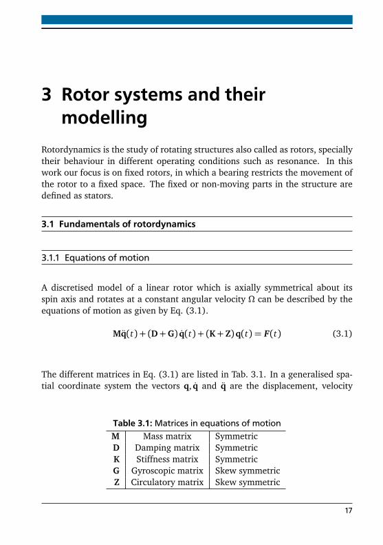
Table 3.1: Matrices in equations of motionM Mass matrix SymmetricD Damping matrix SymmetricK Stiffness matrix SymmetricG Gyroscopic matrix Skew symmetricZ Circulatory matrix Skew symmetric

17

and acceleration vectors respectively in time domain. In the generalised sys-tem, torsional Degrees of freedom (DOF) and axial displacement (x) can beneglected. So only two dimensional displacement in lateral directions (z,y)and two dimensional rotations (ϕx ,ϕy) are considered. The above mentionedvectors has hence four quantities per node. The vector F(t) is the external forceon the system, which in rotordynamics is predominantly the residual unbalanceforce.

The matrix Z is significant in a rotor mounted on hydrodynamic bearings orwith seals, where the damping of fluid film surrounding the rotor plays a role.The matrix G contains only inertial terms which are associated with gyroscopicmoments acting on the rotating parts of a system. If the equation is written ina non-inertial frame, the matrix includes components of Coriolis acceleration.The rotor is not only a point mass, but also has principal moments of inertia.

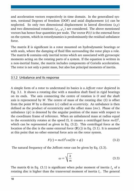
3.1.2 Unbalance and its response

A simple form of a rotor to understand its basics is a Jeffcott rotor depicted inFig. 3.1. It shows a rotating disc with a massless shaft fixed in rigid bearingson its ends. The axis connecting the centre of rotation is O and the shaftaxis is represented by W. The centre of mass of the rotating disc (S) is offsetfrom the point W by a distance (ε) called as eccentricity. An unbalance is thendefined as the product of eccentricity and the offset mass (mε). Phase of theunbalance (φ) is denoted by the angular position of the mass with respect tothe coordinate frame of reference. When an unbalanced mass at radius equalto the eccentricity rotates at the speed Ω, it causes a centrifugal force mεΩ2,which can be represented as given in Eq. (3.2). This centrifugal force at thelocation of the disc is the same external force (F(t)) in Eq. (3.1). It is assumedat this point that no other external force acts on the rotor system.

F(t) = mεΩ2cos(Ωt +φ) (3.2)

The natural frequency of the Jeffcott rotor can be given by Eq. (3.3).

ω=

√

√ km

(3.3)

The matrix G in Eq. (3.1) is significant when polar moment of inertia Ip of arotating disc is higher than the transversal moment of inertia It . The general

18

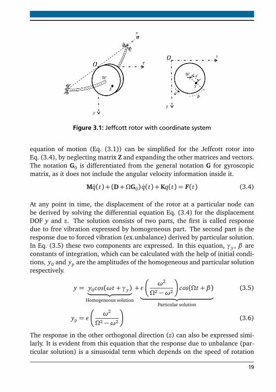
Figure 3.1: Jeffcott rotor with coordinate system

equation of motion (Eq. (3.1)) can be simplified for the Jeffcott rotor intoEq. (3.4), by neglecting matrix Z and expanding the other matrices and vectors.The notation G0 is differentiated from the general notation G for gyroscopicmatrix, as it does not include the angular velocity information inside it.

Mq(t) + (D+ΩG0) q(t) +Kq(t) = F(t) (3.4)

At any point in time, the displacement of the rotor at a particular node canbe derived by solving the differential equation Eq. (3.4) for the displacementDOF y and z. The solution consists of two parts, the first is called responsedue to free vibration expressed by homogeneous part. The second part is theresponse due to forced vibration (ex.unbalance) derived by particular solution.In Eq. (3.5) these two components are expressed. In this equation, γy , β areconstants of integration, which can be calculated with the help of initial condi-tions, y0 and yp are the amplitudes of the homogeneous and particular solutionrespectively.

y = y0cos(ωt + γy)︸ ︷︷ ︸

Homogeneous solution

+ε

ω2

Ω2 −ω2

cos(Ωt + β)︸ ︷︷ ︸

Particular solution

(3.5)

yp = ε

ω2

Ω2 −ω2

(3.6)

The response in the other orthogonal direction (z) can also be expressed simi-larly. It is evident from this equation that the response due to unbalance (par-ticular solution) is a sinusoidal term which depends on the speed of rotation

19

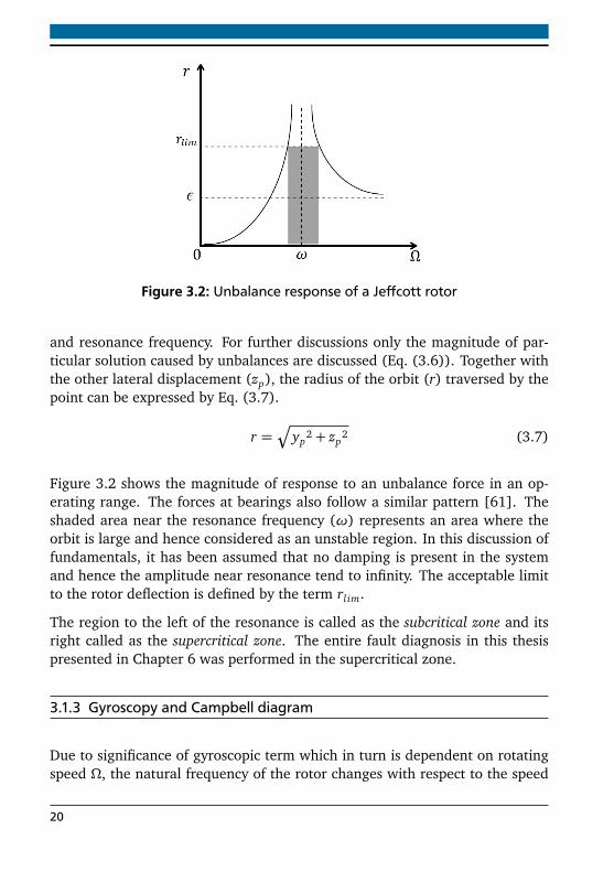
Figure 3.2: Unbalance response of a Jeffcott rotor

and resonance frequency. For further discussions only the magnitude of par-ticular solution caused by unbalances are discussed (Eq. (3.6)). Together withthe other lateral displacement (zp), the radius of the orbit (r) traversed by thepoint can be expressed by Eq. (3.7).

r =q

yp2 + zp

2 (3.7)

Figure 3.2 shows the magnitude of response to an unbalance force in an op-erating range. The forces at bearings also follow a similar pattern [61]. Theshaded area near the resonance frequency (ω) represents an area where theorbit is large and hence considered as an unstable region. In this discussion offundamentals, it has been assumed that no damping is present in the systemand hence the amplitude near resonance tend to infinity. The acceptable limitto the rotor deflection is defined by the term rl im.

The region to the left of the resonance is called as the subcritical zone and itsright called as the supercritical zone. The entire fault diagnosis in this thesispresented in Chapter 6 was performed in the supercritical zone.

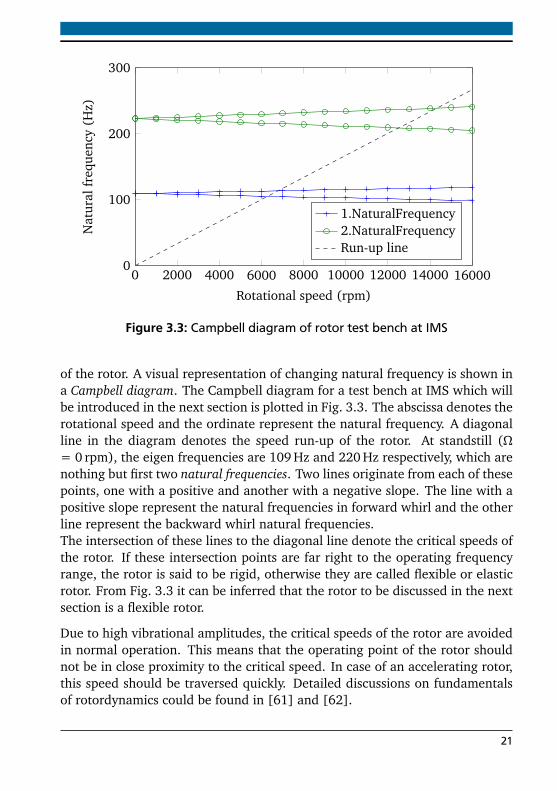
3.1.3 Gyroscopy and Campbell diagram

Due to significance of gyroscopic term which in turn is dependent on rotatingspeed Ω, the natural frequency of the rotor changes with respect to the speed

20

0 2000 4000 6000 8000 10000 12000 14000 160000

100

200

300

Rotational speed (rpm)

Nat

ural

freq

uenc

y(H

z)

1.NaturalFrequency2.NaturalFrequencyRun-up line

Figure 3.3: Campbell diagram of rotor test bench at IMS

of the rotor. A visual representation of changing natural frequency is shown ina Campbell diagram. The Campbell diagram for a test bench at IMS which willbe introduced in the next section is plotted in Fig. 3.3. The abscissa denotes therotational speed and the ordinate represent the natural frequency. A diagonalline in the diagram denotes the speed run-up of the rotor. At standstill (Ω= 0 rpm), the eigen frequencies are 109 Hz and 220 Hz respectively, which arenothing but first two natural frequencies. Two lines originate from each of thesepoints, one with a positive and another with a negative slope. The line with apositive slope represent the natural frequencies in forward whirl and the otherline represent the backward whirl natural frequencies.The intersection of these lines to the diagonal line denote the critical speeds ofthe rotor. If these intersection points are far right to the operating frequencyrange, the rotor is said to be rigid, otherwise they are called flexible or elasticrotor. From Fig. 3.3 it can be inferred that the rotor to be discussed in the nextsection is a flexible rotor.

Due to high vibrational amplitudes, the critical speeds of the rotor are avoidedin normal operation. This means that the operating point of the rotor shouldnot be in close proximity to the critical speed. In case of an accelerating rotor,this speed should be traversed quickly. Detailed discussions on fundamentalsof rotordynamics could be found in [61] and [62].

21

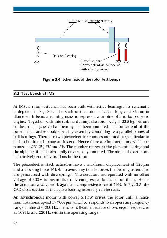
Figure 3.4: Schematic of the rotor test bench

3.2 Test bench at IMS

At IMS, a rotor testbench has been built with active bearings. Its schematicis depicted in Fig. 3.4. The shaft of the rotor is 1.17 m long and 35 mm indiameter. It bears a rotating mass to represent a turbine of a turbo propellerengine. Together with this turbine dummy, the rotor weighs 22.5 kg. At oneof the sides a passive ball-bearing has been mounted. The other end of therotor has an active double bearing assembly containing two parallel planes ofball bearings. There are two piezoelectric actuators mounted perpendicular toeach other in each plane at this end. Hence there are four actuators which arenamed as 2H, 2V, 3H and 3V. The number represent the plane of bearing andthe alphabet if it is horizontally or vertically mounted. The aim of the actuatorsis to actively control vibrations in the rotor.

The piezoelectric stack actuators have a maximum displacement of 120µmand a blocking force 14 kN. To avoid any tensile forces the bearing assembliesare prestressed with disc springs. The actuators are operated with an offsetvoltage of 500 V to ensure that only compressive forces act on them. Hencethe actuators always work against a compressive force of 7 kN. In Fig. 3.5, theCAD cross section of the active bearing assembly can be seen.

An asynchronous motor with power 5.1 kW drives the rotor until a maxi-mum rotational speed 17700 rpm which corresponds to an operating frequencyrange of almost 0-300 Hz.The rotor is flexible because of two eigen frequenciesat 109 Hz and 220 Hz within the operating range.

22

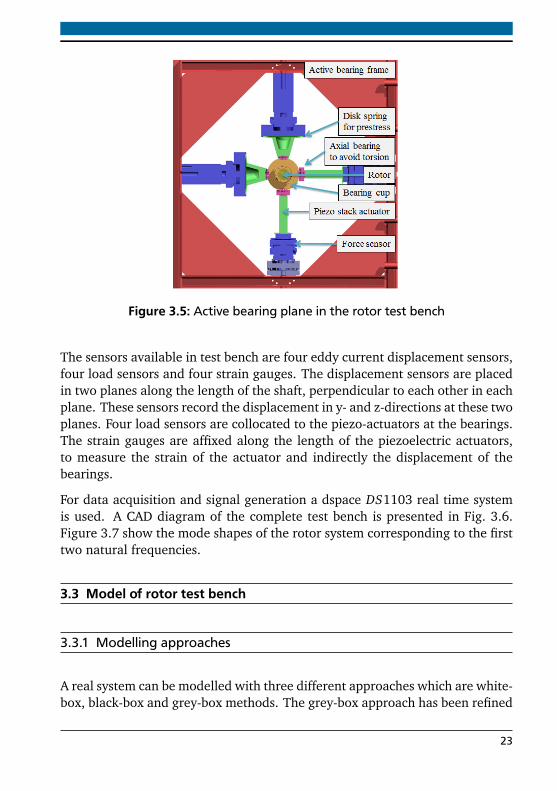
Figure 3.5: Active bearing plane in the rotor test bench

The sensors available in test bench are four eddy current displacement sensors,four load sensors and four strain gauges. The displacement sensors are placedin two planes along the length of the shaft, perpendicular to each other in eachplane. These sensors record the displacement in y- and z-directions at these twoplanes. Four load sensors are collocated to the piezo-actuators at the bearings.The strain gauges are affixed along the length of the piezoelectric actuators,to measure the strain of the actuator and indirectly the displacement of thebearings.

For data acquisition and signal generation a dspace DS1103 real time systemis used. A CAD diagram of the complete test bench is presented in Fig. 3.6.Figure 3.7 show the mode shapes of the rotor system corresponding to the firsttwo natural frequencies.

3.3 Model of rotor test bench

3.3.1 Modelling approaches

A real system can be modelled with three different approaches which are white-box, black-box and grey-box methods. The grey-box approach has been refined

23

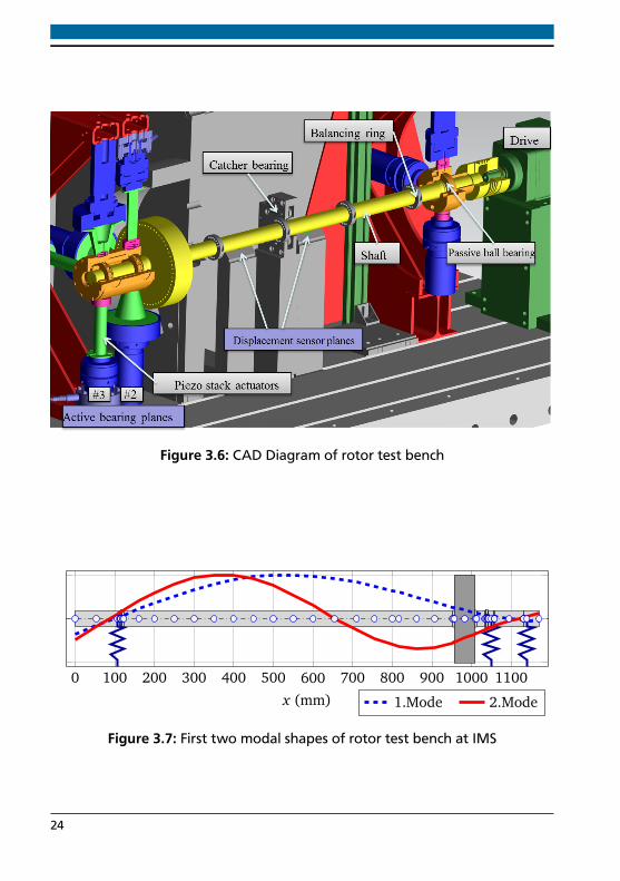
Figure 3.6: CAD Diagram of rotor test bench

0 100 200 300 400 500 600 700 800 900 1000 1100

x (mm) 1.Mode 2.Mode

Figure 3.7: First two modal shapes of rotor test bench at IMS

24

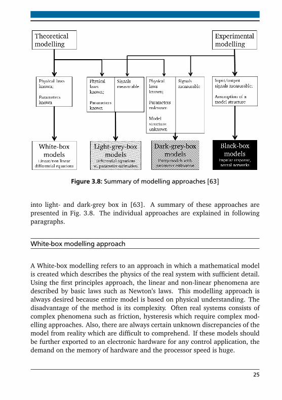
Figure 3.8: Summary of modelling approaches [63]

into light- and dark-grey box in [63]. A summary of these approaches arepresented in Fig. 3.8. The individual approaches are explained in followingparagraphs.

White-box modelling approach

A White-box modelling refers to an approach in which a mathematical modelis created which describes the physics of the real system with sufficient detail.Using the first principles approach, the linear and non-linear phenomena aredescribed by basic laws such as Newton’s laws. This modelling approach isalways desired because entire model is based on physical understanding. Thedisadvantage of the method is its complexity. Often real systems consists ofcomplex phenomena such as friction, hysteresis which require complex mod-elling approaches. Also, there are always certain unknown discrepancies of themodel from reality which are difficult to comprehend. If these models shouldbe further exported to an electronic hardware for any control application, thedemand on the memory of hardware and the processor speed is huge.

25

Black-box modelling approach

Another commonly used modelling approach is the black-box method. In thismethod, a model is constructed without the system knowledge but based onmeasured data from a real system. The commonly used methods are neuralnetworks, Hammerstein-Wiener models to build a black-box model. The dis-advantage of this method is the necessity of large amount of data coveringthe entire operating range of the machine (e.g. complete frequency range)and also considering all the influencing parameters (e.g. Temperature of theenvironment).

Inorder to generate a black-box model for the rotor system, it needs to be run atdifferent stationary rotational frequencies with different unbalances, and alsoby applying a chirp signal at each operating point. Also an intuition to under-stand the fundamentals of the real rotor system would be lost. This approachis not used to generate a model because of its dependency on huge data.

Grey-box modelling approach

As illustrated in Fig. 3.8, a grey-box approach is a combination of the abovetwo approaches. Here a basic model would be created by physical principles.The real system will be subjected to certain test input signals and output mea-sured. If there are deficiencies in the model with respect to the measured datafrom the real system, they will be completed by means of methods such asparameter estimation with the help of an optimisation routine. Based on theextent of physical knowledge available, they can be differentiated into a light-or dark-grey-box models. In the present work, a light-grey-box approach isbeing used. The physical model is explained in Section 3.3.2 and the transferfunction estimation from test bench in Section 3.4.1. The grey-box approachand the final transfer functions of the test bench are presented subsequently.

3.3.2 FE model of rotor test bench

In IMS, a toolbox called rotorbuild had been developed and implemented inMATLAB. This toolbox constructs FE model of rotor systems based on Timo-shenko beam theory. The first mathematical model of the test bench has been

26

constructed in [4] from this toolbox. In this work, the rotor shaft and the activebearings are modelled separately and then integrated.

Modelling the rotor

The rotating parts in test bench are a shaft and the turbine dummy. The shaftwas discretised into smaller beam elements and their individual mass, stiffnessand moment of inertia are calculated based on their material and geometricproperties. Similarly the properties of rotating turbine dummy were also cal-culated. The turbine mass is fitted to shaft by shrink fit. In order to model thefit, an elasticity constant was initially assumed and later estimated by compar-ing it with modal data.

Active bearing model

As presented in Section 3.2, in the test bench an active double bearing ismounted on one of the sides. The ball bearing in each plane is supportedby piezoelectric actuators in perpendicular directions. To avoid any tensileforces in the actuators they are pre-stressed by disc springs. In Fig. 3.9, a verti-cal cross section of the assembly shows one of the actuator and its prestressedsetup, and their respective parameters, which are listed in Tab. 3.2. Fig. 3.10shows the model of double bearing setup, where the cross section in one of thedirections shows both bearing planes. The initial parameters according to [4]were improved by [64] using modal updating methods. Six DOF are depictedin this figure. Considering the other perpendicular place, totally there are 12DOF in the active bearing model. This model has been used further in thisresearch work.

3.3.3 Integrated FE model

The complete model including the rotor and bearings consist of 57 finite ele-ment nodes. With four DOF per node, there are totally 228 degrees of freedom.The mass and stiffness of most of the nodes are calculated from their materialproperties and geometric data. A proportional damping has been assumed inthis model as given in Eq. (3.8). The proportional factors are identified by

27

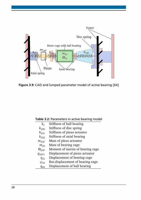
Figure 3.9: CAD and lumped parameter model of active bearing [64]

Table 3.2: Parameters in active bearing modelkL Stiffness of ball bearing

k230 Stiffness of disc springk231 Stiffness of piezo actuatork232 Stiffness of axial bearing

m23P Mass of piezo actuatorm23 Mass of bearing cageΘ23P Moment of inertia of bearing cageq23P1 Displacement of piezo actuator

q23 Displacement of bearing cageϕ23 Rot.displacement of bearing cageqR2 Displacement of ball bearing

28

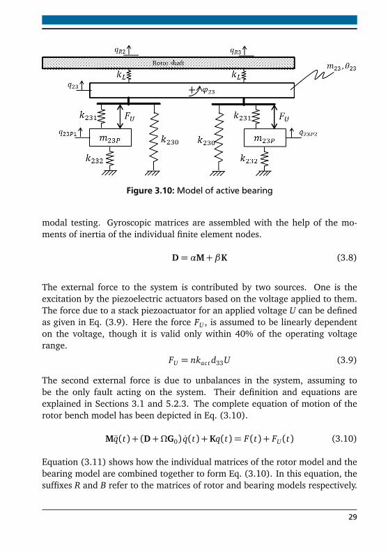
Figure 3.10: Model of active bearing

modal testing. Gyroscopic matrices are assembled with the help of the mo-ments of inertia of the individual finite element nodes.

D= αM+ βK (3.8)

The external force to the system is contributed by two sources. One is theexcitation by the piezoelectric actuators based on the voltage applied to them.The force due to a stack piezoactuator for an applied voltage U can be definedas given in Eq. (3.9). Here the force FU , is assumed to be linearly dependenton the voltage, though it is valid only within 40% of the operating voltagerange.

FU = nkact d33U (3.9)

The second external force is due to unbalances in the system, assuming tobe the only fault acting on the system. Their definition and equations areexplained in Sections 3.1 and 5.2.3. The complete equation of motion of therotor bench model has been depicted in Eq. (3.10).

Mq(t) + (D+ΩG0) q(t) +Kq(t) = F(t) + FU(t) (3.10)

Equation (3.11) shows how the individual matrices of the rotor model and thebearing model are combined together to form Eq. (3.10). In this equation, thesuffixes R and B refer to the matrices of rotor and bearing models respectively.

29

Matrix Kc refers to the matrix containing stiffness values at the DOF where therotor and bearing are coupled.

MR 00 M B

q(t)+

D+Ω

GR 00 0

q(t)+

KR KcK T

c KB

q(t) = F(t)+FU(t)

(3.11)This model can be expressed in a state space representation as given inEq. (3.12).

qq

=

0 I−M−1K −M−1(D+ΩG0)

qq

+

0M−1

F +

0M−1

FU

q = [I 0]

qq

(3.12)

3.4 Model enhancement with measured data

The basic structure of the rotor system which was created in [4], needs to becorrected for its accuracy at different frequency positions and also for correctnatural frequencies. The model has then been constantly improved for betteraccuracy in different works such as [65], [66] and in [64]. The transfer func-tions from measured data are compared to those generated from mathematicalmodel. The differences between them was minimised by different grey-boxmodelling approaches.

In Section 3.4.1, method to estimate transfer function from measured signalsis explained along with the description about the measurements done in thetest bench. The model enhancement procedure is explained subsequently inSection 3.4.2. Finally the complete model is presented in Section 3.4.3.

3.4.1 Transfer function estimation from measured data

Estimation

The procedure to estimate the transfer function between any two measuredsignals according to [67] has been described below in Eq. (3.13)-(3.17). Herethe vector Sx x refer to the spectral power density of signal x . The spectral

30

density between the signals p and x are referred as cross-spectral density Spx .

H4(Ω) = [1− κ (Ω)]H1(Ω) +κ (Ω)H2(Ω) (3.13)

κ (Ω) =H3(Ω)

maxΩ |H3(Ω)|(3.14)

H1(Ω) =Spx (Ω)

Spp (Ω)(3.15)

H2(Ω) =Sx x (Ω)Sx p (Ω)

(3.16)

H3(Ω) =12(H1(Ω) +H2(Ω)) (3.17)

With the help of the variable Cx y in Eq. (3.18), the coherence between thesignals x and y can be measured.

Cx y (Ω) =

Sx y (Ω)

2

Sx x (Ω)Sy y (Ω)(3.18)

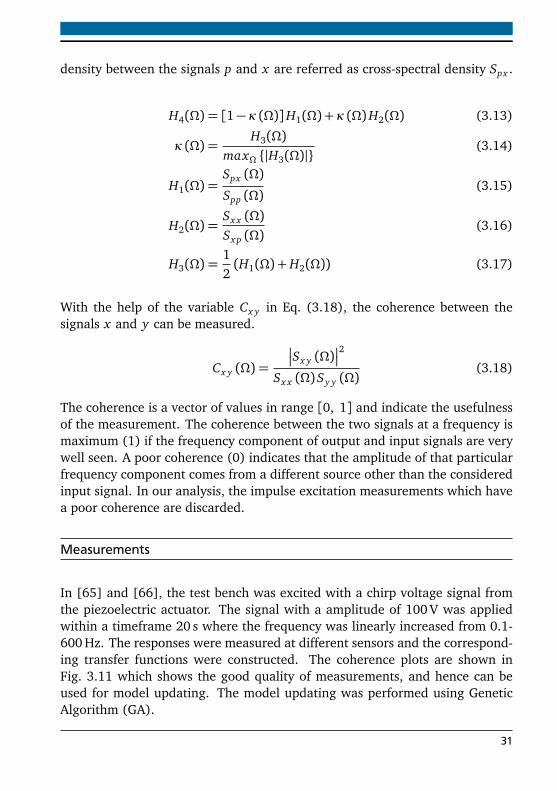
The coherence is a vector of values in range [0, 1] and indicate the usefulnessof the measurement. The coherence between the two signals at a frequency ismaximum (1) if the frequency component of output and input signals are verywell seen. A poor coherence (0) indicates that the amplitude of that particularfrequency component comes from a different source other than the consideredinput signal. In our analysis, the impulse excitation measurements which havea poor coherence are discarded.

Measurements

In [65] and [66], the test bench was excited with a chirp voltage signal fromthe piezoelectric actuator. The signal with a amplitude of 100 V was appliedwithin a timeframe 20 s where the frequency was linearly increased from 0.1-600 Hz. The responses were measured at different sensors and the correspond-ing transfer functions were constructed. The coherence plots are shown inFig. 3.11 which shows the good quality of measurements, and hence can beused for model updating. The model updating was performed using GeneticAlgorithm (GA).

31

0 50 100 150 200 250 3000

0.2

0.4

0.6

0.8

1

Frequency (Hz)

Coh

eren

ce

FU to Displ1FU to Displ2FU to Force

Figure 3.11: Coherence from chirp voltage to all sensors

Figure 3.12: Impulse excitation positions in test bench

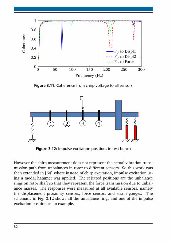
However the chirp measurement does not represent the actual vibration trans-mission path from unbalances in rotor to different sensors. So this work wasthen extended in [64] where instead of chirp excitation, impulse excitation us-ing a modal hammer was applied. The selected positions are the unbalancerings on rotor shaft so that they represent the force transmission due to unbal-ance masses. The responses were measured at all available sensors, namelythe displacement proximity sensors, force sensors and strain gauges. Theschematic in Fig. 3.12 shows all the unbalance rings and one of the impulseexcitation position as an example.

32

2 2.01 2.02

0

500

1000

Time (s)

Impu

lse

Forc

e(N

)

(a) Time domain

0 100 200 30010−2

10−1

100

Frequency (Hz)

Impu

lse

Forc

e(N

)

(b) Frequency domain

Figure 3.13: Impulse hammer excitation

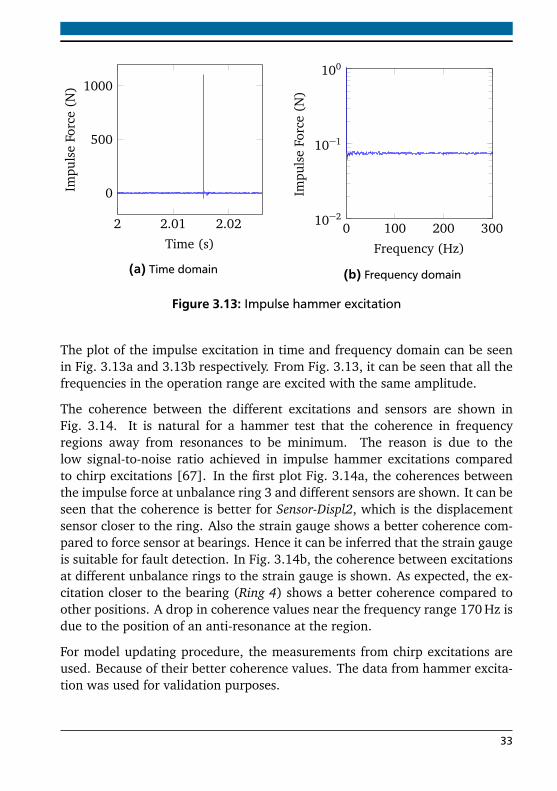
The plot of the impulse excitation in time and frequency domain can be seenin Fig. 3.13a and 3.13b respectively. From Fig. 3.13, it can be seen that all thefrequencies in the operation range are excited with the same amplitude.

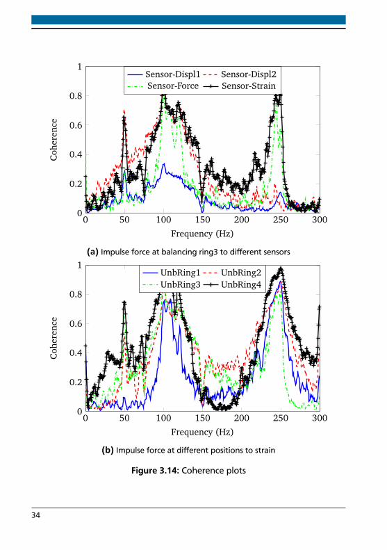
The coherence between the different excitations and sensors are shown inFig. 3.14. It is natural for a hammer test that the coherence in frequencyregions away from resonances to be minimum. The reason is due to thelow signal-to-noise ratio achieved in impulse hammer excitations comparedto chirp excitations [67]. In the first plot Fig. 3.14a, the coherences betweenthe impulse force at unbalance ring 3 and different sensors are shown. It can beseen that the coherence is better for Sensor-Displ2, which is the displacementsensor closer to the ring. Also the strain gauge shows a better coherence com-pared to force sensor at bearings. Hence it can be inferred that the strain gaugeis suitable for fault detection. In Fig. 3.14b, the coherence between excitationsat different unbalance rings to the strain gauge is shown. As expected, the ex-citation closer to the bearing (Ring 4) shows a better coherence compared toother positions. A drop in coherence values near the frequency range 170 Hz isdue to the position of an anti-resonance at the region.

For model updating procedure, the measurements from chirp excitations areused. Because of their better coherence values. The data from hammer excita-tion was used for validation purposes.

33

0 50 100 150 200 250 3000

0.2

0.4

0.6

0.8

1

Frequency (Hz)

Coh

eren

ce

Sensor-Displ1 Sensor-Displ2Sensor-Force Sensor-Strain

(a) Impulse force at balancing ring3 to different sensors

0 50 100 150 200 250 3000

0.2

0.4

0.6

0.8

1

Frequency (Hz)

Coh

eren

ce

UnbRing1 UnbRing2UnbRing3 UnbRing4

(b) Impulse force at different positions to strain

Figure 3.14: Coherence plots

34

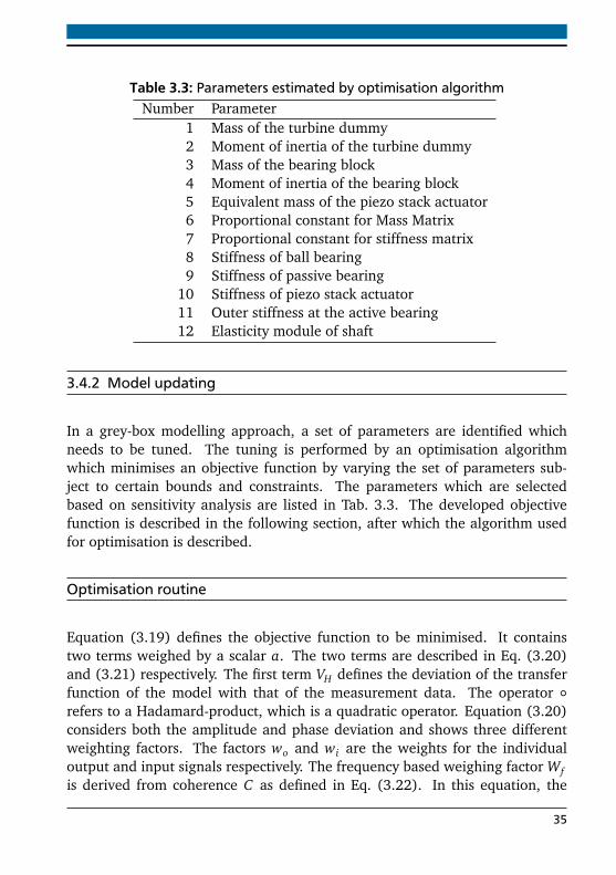
Table 3.3: Parameters estimated by optimisation algorithmNumber Parameter

1 Mass of the turbine dummy2 Moment of inertia of the turbine dummy3 Mass of the bearing block4 Moment of inertia of the bearing block5 Equivalent mass of the piezo stack actuator6 Proportional constant for Mass Matrix7 Proportional constant for stiffness matrix8 Stiffness of ball bearing9 Stiffness of passive bearing

10 Stiffness of piezo stack actuator11 Outer stiffness at the active bearing12 Elasticity module of shaft

3.4.2 Model updating

In a grey-box modelling approach, a set of parameters are identified whichneeds to be tuned. The tuning is performed by an optimisation algorithmwhich minimises an objective function by varying the set of parameters sub-ject to certain bounds and constraints. The parameters which are selectedbased on sensitivity analysis are listed in Tab. 3.3. The developed objectivefunction is described in the following section, after which the algorithm usedfor optimisation is described.

Optimisation routine

Equation (3.19) defines the objective function to be minimised. It containstwo terms weighed by a scalar a. The two terms are described in Eq. (3.20)and (3.21) respectively. The first term VH defines the deviation of the transferfunction of the model with that of the measurement data. The operator refers to a Hadamard-product, which is a quadratic operator. Equation (3.20)considers both the amplitude and phase deviation and shows three differentweighting factors. The factors wo and wi are the weights for the individualoutput and input signals respectively. The frequency based weighing factor Wfis derived from coherence C as defined in Eq. (3.22). In this equation, the

35

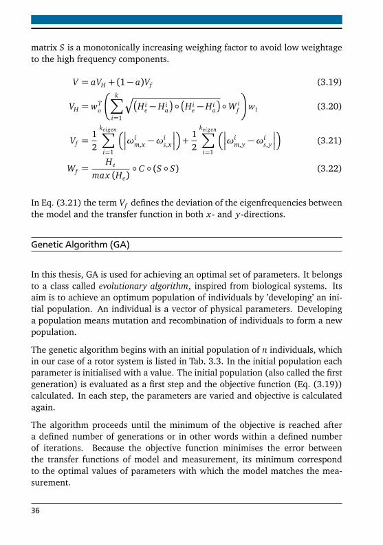
matrix S is a monotonically increasing weighing factor to avoid low weightageto the high frequency components.

V = aVH + (1− a)Vf (3.19)

VH = wTo

k∑

i=1

Ç

H ie −H i

a

H ie −H i

a

W if

wi (3.20)

Vf =12

keigen∑

i=1

ωim,x −ω

is,x

+12

keigen∑

i=1

ωim,y −ω

is,y

(3.21)

Wf =He

max (He) C (S S) (3.22)

In Eq. (3.21) the term Vf defines the deviation of the eigenfrequencies betweenthe model and the transfer function in both x- and y-directions.

Genetic Algorithm (GA)

In this thesis, GA is used for achieving an optimal set of parameters. It belongsto a class called evolutionary algorithm, inspired from biological systems. Itsaim is to achieve an optimum population of individuals by ’developing’ an ini-tial population. An individual is a vector of physical parameters. Developinga population means mutation and recombination of individuals to form a newpopulation.

The genetic algorithm begins with an initial population of n individuals, whichin our case of a rotor system is listed in Tab. 3.3. In the initial population eachparameter is initialised with a value. The initial population (also called the firstgeneration) is evaluated as a first step and the objective function (Eq. (3.19))calculated. In each step, the parameters are varied and objective is calculatedagain.

The algorithm proceeds until the minimum of the objective is reached aftera defined number of generations or in other words within a defined numberof iterations. Because the objective function minimises the error betweenthe transfer functions of model and measurement, its minimum correspondto the optimal values of parameters with which the model matches the mea-surement.

36

3.4.3 Complete model of the test bench

The result of the model updating can be seen from FRF plot in Fig. 3.15aand Fig. 3.15b. The initial model before update has also been compared toshow the effectiveness of the model updating procedure. In Fig. 3.15a theFRF identified from the model was compared to identified transfer functionobtained by chirp excitation of the structure. (FRF of piezoelectric actuatorvoltage to the force sensor collocated to it). For the sake of comparison, FRFidentified from impulse excitations are plotted against the model in Fig. 3.15b.It can be seen that in both magnitude and phase, the model is able to followthe identified FRF closely. Also the resonance frequencies are located veryprecisely. A good approximation to the real behaviour can be seen.

3.5 Aircraft turbofan engine

The aircraft engine which is being diagnosed for faults is a twin-spool engineused for business jets, a picture of which is presented in Fig. 3.16a. In today’sdate, jet propulsion is often linked with gas turbine engine. A simple descrip-tion of mechanical construction of the gas turbine engine is that, it consists oftwo coaxial rotating shafts with compressor and turbine stages, and stationarycombustion chambers between them. The axial flow compressors with multi-ple stages are assembled in two rotors, the LP and HP shafts, where the airis compressed gradually at each stage. A stage consists of a row of rotatingblades followed by a row of stator vanes, which vary the air flow directionsdepending on the operating point of the compressor. Each compressor rotor isdriven by its own turbine. In Fig. 3.16b, the schematic of the twin spool jetengine is shown, where the LP and HP rotor have their own compressor andturbine stages.

The construction of the compressor centres around the rotor assembly and cas-ings. The rotor shafts are supported in rolling element bearings on either side.The LP compressor is supported by one more bearing at the front, as a safetyaspect against bird-hit.

The balancing of a compressor rotor is an extremely important operation inits manufacture. Because of the high rotational speeds and the mass of therotating components high unbalance forces are resulted. These forces wouldaffect the bearings and engine operation. To minimise the effect of dynamic

37

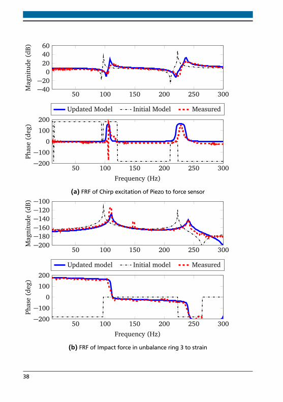
50 100 150 200 250 300−40−20

0204060

Mag

nitu

de(d

B)

50 100 150 200 250 300−200

−100

0

100

200

Frequency (Hz)

Phas

e(d

eg)

Updated Model Initial Model Measured

(a) FRF of Chirp excitation of Piezo to force sensor

50 100 150 200 250 300−200−180−160−140−120−100

Mag

nitu

de(d

B)

50 100 150 200 250 300−200

−100

0

100

200

Frequency (Hz)

Phas

e(d

eg)

Updated model Initial model Measured

(b) FRF of Impact force in unbalance ring 3 to strain

38

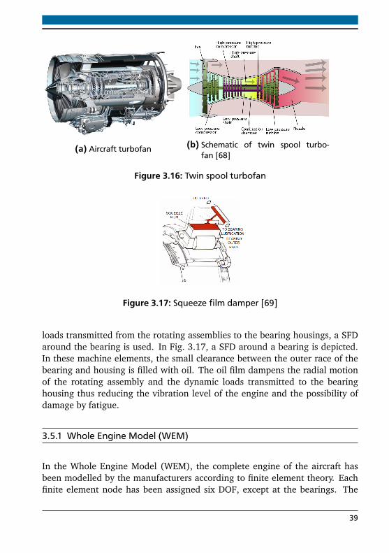
(a) Aircraft turbofan (b) Schematic of twin spool turbo-fan [68]

Figure 3.16: Twin spool turbofan

Figure 3.17: Squeeze film damper [69]

loads transmitted from the rotating assemblies to the bearing housings, a SFDaround the bearing is used. In Fig. 3.17, a SFD around a bearing is depicted.In these machine elements, the small clearance between the outer race of thebearing and housing is filled with oil. The oil film dampens the radial motionof the rotating assembly and the dynamic loads transmitted to the bearinghousing thus reducing the vibration level of the engine and the possibility ofdamage by fatigue.

3.5.1 Whole Engine Model (WEM)

In the Whole Engine Model (WEM), the complete engine of the aircraft hasbeen modelled by the manufacturers according to finite element theory. Eachfinite element node has been assigned six DOF, except at the bearings. The

39

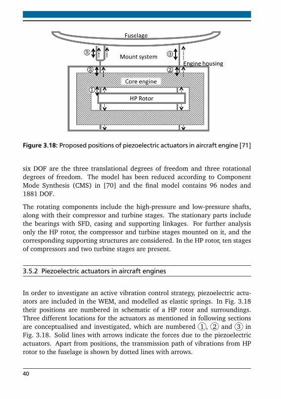
Figure 3.18: Proposed positions of piezoelectric actuators in aircraft engine [71]

six DOF are the three translational degrees of freedom and three rotationaldegrees of freedom. The model has been reduced according to ComponentMode Synthesis (CMS) in [70] and the final model contains 96 nodes and1881 DOF.

The rotating components include the high-pressure and low-pressure shafts,along with their compressor and turbine stages. The stationary parts includethe bearings with SFD, casing and supporting linkages. For further analysisonly the HP rotor, the compressor and turbine stages mounted on it, and thecorresponding supporting structures are considered. In the HP rotor, ten stagesof compressors and two turbine stages are present.

3.5.2 Piezoelectric actuators in aircraft engines

In order to investigate an active vibration control strategy, piezoelectric actu-ators are included in the WEM, and modelled as elastic springs. In Fig. 3.18their positions are numbered in schematic of a HP rotor and surroundings.Three different locations for the actuators as mentioned in following sectionsare conceptualised and investigated, which are numbered 1 , 2 and 3 inFig. 3.18. Solid lines with arrows indicate the forces due to the piezoelectricactuators. Apart from positions, the transmission path of vibrations from HProtor to the fuselage is shown by dotted lines with arrows.

40

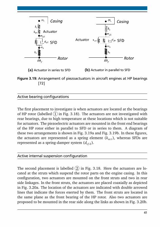
(a) Actuator in series to SFD (b) Actuator in parallel to SFD

Figure 3.19: Arrangement of piezoactuators in aircraft engines at HP bearings[72]

Active bearing configurations

The first placement to investigate is when actuators are located at the bearingsof HP rotor (labelled 1 in Fig. 3.18). The actuators are not investigated withrear bearings, due to high temperature at these locations which is not suitablefor actuators. The piezoelectric actuators are mounted in the front end bearingsof the HP rotor either in parallel to SFD or in series to them. A diagram ofthese two arrangements is shown in Fig. 3.19a and Fig. 3.19b. In these figures,the actuators are represented as a spring element (kact), whereas SFDs arerepresented as a spring-damper system (ds f d).

Active internal suspension configuration

The second placement is labelled 2 in Fig. 3.18. Here the actuators are lo-cated at the struts which suspend the rotor parts on the engine casing. In thisconfiguration, two actuators are mounted on the front struts and two in rearside linkages. In the front struts, the actuators are placed coaxially as depictedin Fig. 3.20a. The location of the actuators are indicated with double arrowedlines that indicate the forces exerted by them. The front struts are located inthe same plane as the front bearing of the HP rotor. Also two actuators areproposed to be mounted in the rear side along the links as shown in Fig. 3.20b.

41

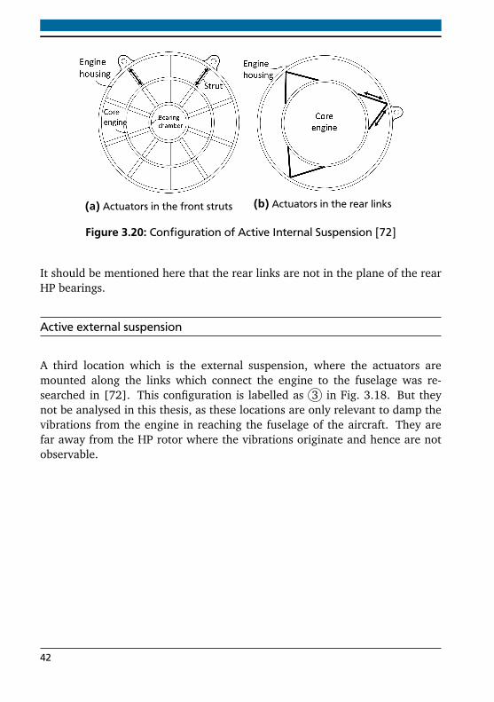
(a) Actuators in the front struts (b) Actuators in the rear links

Figure 3.20: Configuration of Active Internal Suspension [72]

It should be mentioned here that the rear links are not in the plane of the rearHP bearings.

Active external suspension

A third location which is the external suspension, where the actuators aremounted along the links which connect the engine to the fuselage was re-searched in [72]. This configuration is labelled as 3 in Fig. 3.18. But theynot be analysed in this thesis, as these locations are only relevant to damp thevibrations from the engine in reaching the fuselage of the aircraft. They arefar away from the HP rotor where the vibrations originate and hence are notobservable.

42

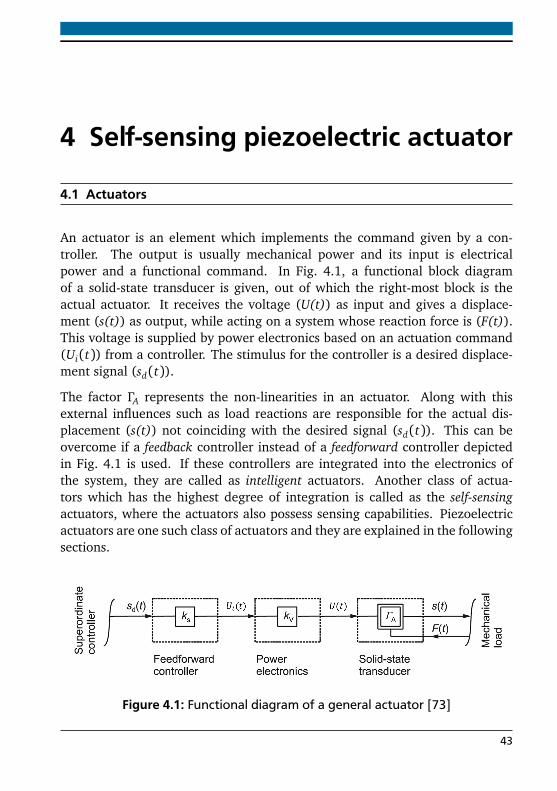
4 Self-sensing piezoelectric actuator

4.1 Actuators

An actuator is an element which implements the command given by a con-troller. The output is usually mechanical power and its input is electricalpower and a functional command. In Fig. 4.1, a functional block diagramof a solid-state transducer is given, out of which the right-most block is theactual actuator. It receives the voltage (U(t)) as input and gives a displace-ment (s(t)) as output, while acting on a system whose reaction force is (F(t)).This voltage is supplied by power electronics based on an actuation command(Ui(t)) from a controller. The stimulus for the controller is a desired displace-ment signal (sd(t)).

The factor ΓA represents the non-linearities in an actuator. Along with thisexternal influences such as load reactions are responsible for the actual dis-placement (s(t)) not coinciding with the desired signal (sd(t)). This can beovercome if a feedback controller instead of a feedforward controller depictedin Fig. 4.1 is used. If these controllers are integrated into the electronics ofthe system, they are called as intelligent actuators. Another class of actua-tors which has the highest degree of integration is called as the self-sensingactuators, where the actuators also possess sensing capabilities. Piezoelectricactuators are one such class of actuators and they are explained in the followingsections.

Figure 4.1: Functional diagram of a general actuator [73]

43

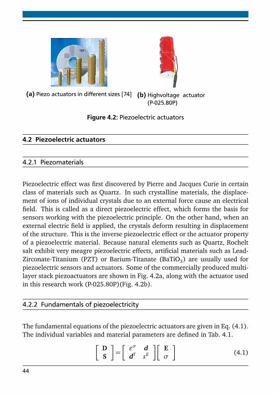
(a) Piezo actuators in different sizes [74] (b) Highvoltage actuator(P-025.80P)

Figure 4.2: Piezoelectric actuators

4.2 Piezoelectric actuators

4.2.1 Piezomaterials

Piezoelectric effect was first discovered by Pierre and Jacques Curie in certainclass of materials such as Quartz. In such crystalline materials, the displace-ment of ions of individual crystals due to an external force cause an electricalfield. This is called as a direct piezoelectric effect, which forms the basis forsensors working with the piezoelectric principle. On the other hand, when anexternal electric field is applied, the crystals deform resulting in displacementof the structure. This is the inverse piezoelectric effect or the actuator propertyof a piezoelectric material. Because natural elements such as Quartz, Rocheltsalt exhibit very meagre piezoelectric effects, artificial materials such as Lead-Zirconate-Titanium (PZT) or Barium-Titanate (BaTiO3) are usually used forpiezoelectric sensors and actuators. Some of the commercially produced multi-layer stack piezoactuators are shown in Fig. 4.2a, along with the actuator usedin this research work (P-025.80P)(Fig. 4.2b).

4.2.2 Fundamentals of piezoelectricity

The fundamental equations of the piezoelectric actuators are given in Eq. (4.1).The individual variables and material parameters are defined in Tab. 4.1.

DS

=

εσ ddT sE

Eσ

(4.1)

44

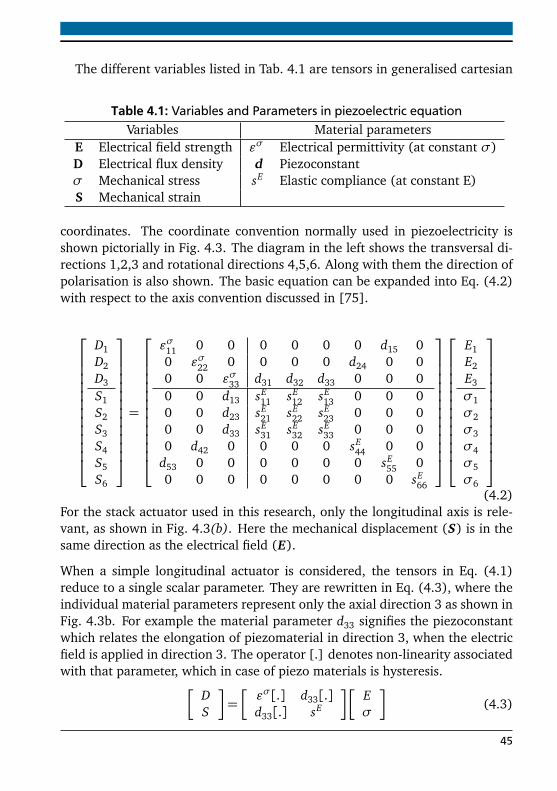
The different variables listed in Tab. 4.1 are tensors in generalised cartesian

Table 4.1: Variables and Parameters in piezoelectric equationVariables Material parameters

E Electrical field strength εσ Electrical permittivity (at constant σ)D Electrical flux density d Piezoconstantσ Mechanical stress sE Elastic compliance (at constant E)S Mechanical strain

coordinates. The coordinate convention normally used in piezoelectricity isshown pictorially in Fig. 4.3. The diagram in the left shows the transversal di-rections 1,2,3 and rotational directions 4,5,6. Along with them the direction ofpolarisation is also shown. The basic equation can be expanded into Eq. (4.2)with respect to the axis convention discussed in [75].

D1D2D3

S1S2S3S4S5S6

=

εσ11 0 0 0 0 0 0 d15 00 εσ22 0 0 0 0 d24 0 00 0 εσ33 d31 d32 d33 0 0 00 0 d13 sE

11 sE12 sE

13 0 0 00 0 d23 sE

21 sE22 sE

23 0 0 00 0 d33 sE

31 sE32 sE

33 0 0 00 d42 0 0 0 0 sE

44 0 0d53 0 0 0 0 0 0 sE

55 00 0 0 0 0 0 0 0 sE

66

E1E2E3

σ1σ2σ3σ4σ5σ6

(4.2)For the stack actuator used in this research, only the longitudinal axis is rele-vant, as shown in Fig. 4.3(b). Here the mechanical displacement (S) is in thesame direction as the electrical field (E).

When a simple longitudinal actuator is considered, the tensors in Eq. (4.1)reduce to a single scalar parameter. They are rewritten in Eq. (4.3), where theindividual material parameters represent only the axial direction 3 as shown inFig. 4.3b. For example the material parameter d33 signifies the piezoconstantwhich relates the elongation of piezomaterial in direction 3, when the electricfield is applied in direction 3. The operator [.] denotes non-linearity associatedwith that parameter, which in case of piezo materials is hysteresis.

DS

=

εσ[.] d33[.]d33[.] sE

Eσ

(4.3)

45

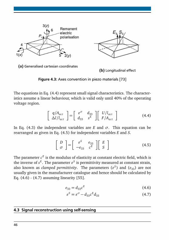
(a) Generalised cartesian coordinates(b) Longitudinal effect

Figure 4.3: Axes convention in piezo materials [73]

The equations in Eq. (4.4) represent small signal characteristics. The character-istics assume a linear behaviour, which is valid only until 40% of the operatingvoltage region.

q/Aact∆l/lact

=

εσ d33d33 sE

U/lactF/Aact

(4.4)

In Eq. (4.3) the independent variables are E and σ. This equation can berearranged as given in Eq. (4.5) for independent variables E and S.

Dσ

=

εS e33−e33 cE

ES

(4.5)

The parameter cE is the modulus of elasticity at constant electric field, which isthe inverse of sE . The parameter εS is permittivity measured at constant strain,also known as clamped permittivity. The parameters (εS) and (e33) are notusually given in the manufacturer catalogue and hence should be calculated byEq. (4.6) - (4.7) assuming linearity [55].

e33 = d33cE (4.6)

εS = εσ − d33cEd33 (4.7)

4.3 Signal reconstruction using self-sensing

46

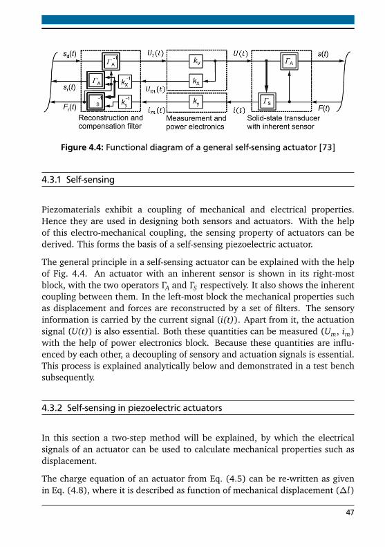
Figure 4.4: Functional diagram of a general self-sensing actuator [73]

4.3.1 Self-sensing

Piezomaterials exhibit a coupling of mechanical and electrical properties.Hence they are used in designing both sensors and actuators. With the helpof this electro-mechanical coupling, the sensing property of actuators can bederived. This forms the basis of a self-sensing piezoelectric actuator.

The general principle in a self-sensing actuator can be explained with the helpof Fig. 4.4. An actuator with an inherent sensor is shown in its right-mostblock, with the two operators ΓA and ΓS respectively. It also shows the inherentcoupling between them. In the left-most block the mechanical properties suchas displacement and forces are reconstructed by a set of filters. The sensoryinformation is carried by the current signal (i(t)). Apart from it, the actuationsignal (U(t)) is also essential. Both these quantities can be measured (Um, im)with the help of power electronics block. Because these quantities are influ-enced by each other, a decoupling of sensory and actuation signals is essential.This process is explained analytically below and demonstrated in a test benchsubsequently.

4.3.2 Self-sensing in piezoelectric actuators

In this section a two-step method will be explained, by which the electricalsignals of an actuator can be used to calculate mechanical properties such asdisplacement.

The charge equation of an actuator from Eq. (4.5) can be re-written as givenin Eq. (4.8), where it is described as function of mechanical displacement (∆l)

47

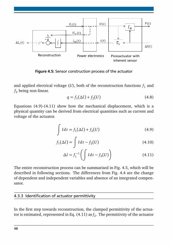
Figure 4.5: Sensor construction process of the actuator

and applied electrical voltage (U), both of the reconstruction functions f1 andf2 being non-linear.

q = f1(∆l) + f2(U) (4.8)

Equations (4.9)-(4.11) show how the mechanical displacement, which is aphysical quantity can be derived from electrical quantities such as current andvoltage of the actuator.

∫

Id t = f1(∆l) + f2(U) (4.9)

f1(∆l) =

∫

Id t − f2(U) (4.10)

∆l = f −11

∫

Id t − f2(U)

(4.11)

The entire reconstruction process can be summarised in Fig. 4.5, which will bedescribed in following sections. The differences from Fig. 4.4 are the changeof dependent and independent variables and absence of an integrated compen-sator.

4.3.3 Identification of actuator permittivity

In the first step towards reconstruction, the clamped permittivity of the actua-tor is estimated, represented in Eq. (4.11) as f2. The permittivity of the actuator

48

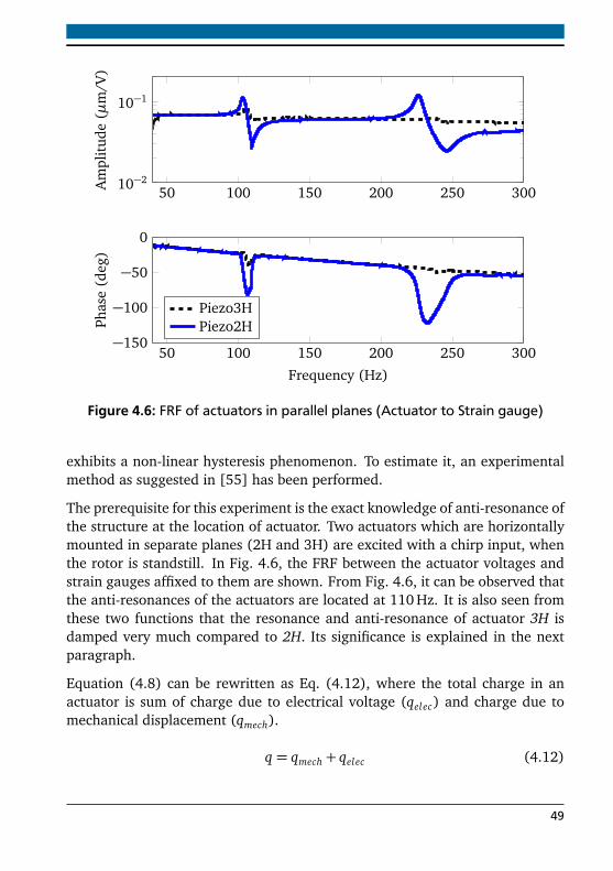
50 100 150 200 250 30010−2

10−1A

mpl

itud

e(µ

m/V

)

50 100 150 200 250 300−150

−100

−50

0

Frequency (Hz)

Phas

e(d

eg)

Piezo3HPiezo2H

Figure 4.6: FRF of actuators in parallel planes (Actuator to Strain gauge)

exhibits a non-linear hysteresis phenomenon. To estimate it, an experimentalmethod as suggested in [55] has been performed.

The prerequisite for this experiment is the exact knowledge of anti-resonance ofthe structure at the location of actuator. Two actuators which are horizontallymounted in separate planes (2H and 3H) are excited with a chirp input, whenthe rotor is standstill. In Fig. 4.6, the FRF between the actuator voltages andstrain gauges affixed to them are shown. From Fig. 4.6, it can be observed thatthe anti-resonances of the actuators are located at 110 Hz. It is also seen fromthese two functions that the resonance and anti-resonance of actuator 3H isdamped very much compared to 2H. Its significance is explained in the nextparagraph.

Equation (4.8) can be rewritten as Eq. (4.12), where the total charge in anactuator is sum of charge due to electrical voltage (qelec) and charge due tomechanical displacement (qmech).

q = qmech + qelec (4.12)

49

Mechanical structures are characterised by resonances and anti-resonances.At the locations of anti-resonances, the mechanical impedance is very highthereby not allowing the system to deform. Hence mechanical displacement(∆l) is very low, which means the quantity qmech is not significant. Accordingto Eq. (4.8), the charge corresponds only to electrical component. Thereforethe permittivity of the actuator is determined at this operating point, because ofno interference from mechanical displacement. Because the anti-resonance ofthe actuator 3H is not well pronounced, it leads to conclude that only actuator2H is useful to identify the permittivity. Because only in actuator 2H at 110 Hz,a complete decoupling of mechanical and electrical signals is possible.

Sinusoidal voltage signals of different amplitudes with frequency equal to theanti-resonance frequency are given to the rotor from the piezoelectric actuator.The voltage and current are measured. The current signal is integrated to givethe charge of the actuator. The permittivity is modelled by the data from thevoltage and charge signal. The hysteresis have been approximated as ellipsesand a curve fitting was performed. The result of hysteresis reconstruction canbe seen in Fig. 4.7, where the charge and voltage of the actuator has beenpresented against that estimated by the model.

Equation (4.10) shows that the current signal should be integrated to derivethe charge signal. Low frequency noise might be present in this signal, whichdistorts the integration. Hence a band-pass filter was implemented digitallyto remove the low frequency disturbance in the current signal. This digitalFinite Impulse Response (FIR) filter allows the signal in the frequency band40-1000 Hz. Because our operating range is only upto 300 Hz, this filter can beassumed to be a high-pass filter. It has its corner frequency 20 Hz and con-structed with an order of 200. This order was chosen to remove the lowfrequency noise within a narrow band 0-20 Hz and have a steep rise in am-plitude response, so that the operating range 50-300 Hz remains unaffected.This is seen in Fig. 4.8, where the magnitude response of the filter has beenplotted. Both the current and voltage are subjected to this high-pass filterduring the self-sensing reconstruction before the curve fitting is performed.

At the position of anti-resonance, the phase of the structure shifts by 180.Hence the precise position of anti-resonance is important, otherwise phasewould be distorted during reconstruction. Hence this method is sensitive toidentification of the anti-resonance frequency.

50

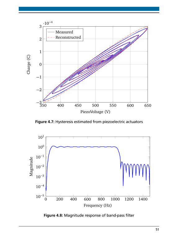
350 400 450 500 550 600 650−3

−2

−1

0

1

2

3·10−4

PiezoVoltage (V)

Cha

rge

(C)

MeasuredReconstructed

Figure 4.7: Hysteresis estimated from piezoelectric actuators

0 200 400 600 800 1000 1200 140010−5

10−4

10−3

10−2

10−1

100

101

Frequency (Hz)

Mag

nitu

de

Figure 4.8: Magnitude response of band-pass filter

51

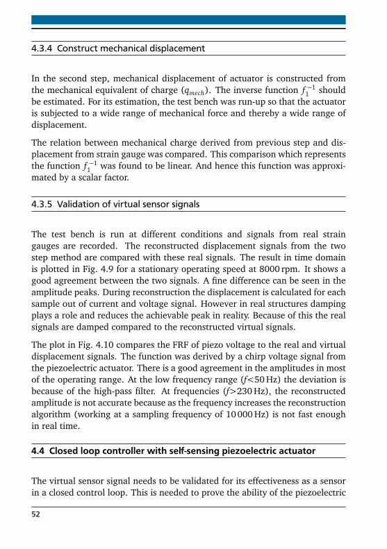
4.3.4 Construct mechanical displacement

In the second step, mechanical displacement of actuator is constructed fromthe mechanical equivalent of charge (qmech). The inverse function f −1

1 shouldbe estimated. For its estimation, the test bench was run-up so that the actuatoris subjected to a wide range of mechanical force and thereby a wide range ofdisplacement.

The relation between mechanical charge derived from previous step and dis-placement from strain gauge was compared. This comparison which representsthe function f −1

1 was found to be linear. And hence this function was approxi-mated by a scalar factor.

4.3.5 Validation of virtual sensor signals

The test bench is run at different conditions and signals from real straingauges are recorded. The reconstructed displacement signals from the twostep method are compared with these real signals. The result in time domainis plotted in Fig. 4.9 for a stationary operating speed at 8000 rpm. It shows agood agreement between the two signals. A fine difference can be seen in theamplitude peaks. During reconstruction the displacement is calculated for eachsample out of current and voltage signal. However in real structures dampingplays a role and reduces the achievable peak in reality. Because of this the realsignals are damped compared to the reconstructed virtual signals.

The plot in Fig. 4.10 compares the FRF of piezo voltage to the real and virtualdisplacement signals. The function was derived by a chirp voltage signal fromthe piezoelectric actuator. There is a good agreement in the amplitudes in mostof the operating range. At the low frequency range (f<50 Hz) the deviation isbecause of the high-pass filter. At frequencies (f>230 Hz), the reconstructedamplitude is not accurate because as the frequency increases the reconstructionalgorithm (working at a sampling frequency of 10 000 Hz) is not fast enoughin real time.

4.4 Closed loop controller with self-sensing piezoelectric actuator

The virtual sensor signal needs to be validated for its effectiveness as a sensorin a closed control loop. This is needed to prove the ability of the piezoelectric

52

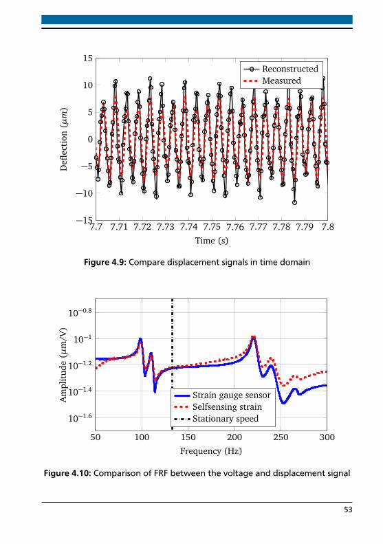
7.7 7.71 7.72 7.73 7.74 7.75 7.76 7.77 7.78 7.79 7.8−15

−10

−5

0

5

10

15

Time (s)

Defl

ecti

on(µ

m)

ReconstructedMeasured

Figure 4.9: Compare displacement signals in time domain

50 100 150 200 250 300

10−1.6

10−1.4

10−1.2

10−1

10−0.8

Frequency (Hz)

Am

plit

ude

(µm

/V)

Strain gauge sensorSelfsensing strainStationary speed

Figure 4.10: Comparison of FRF between the voltage and displacement signal

53

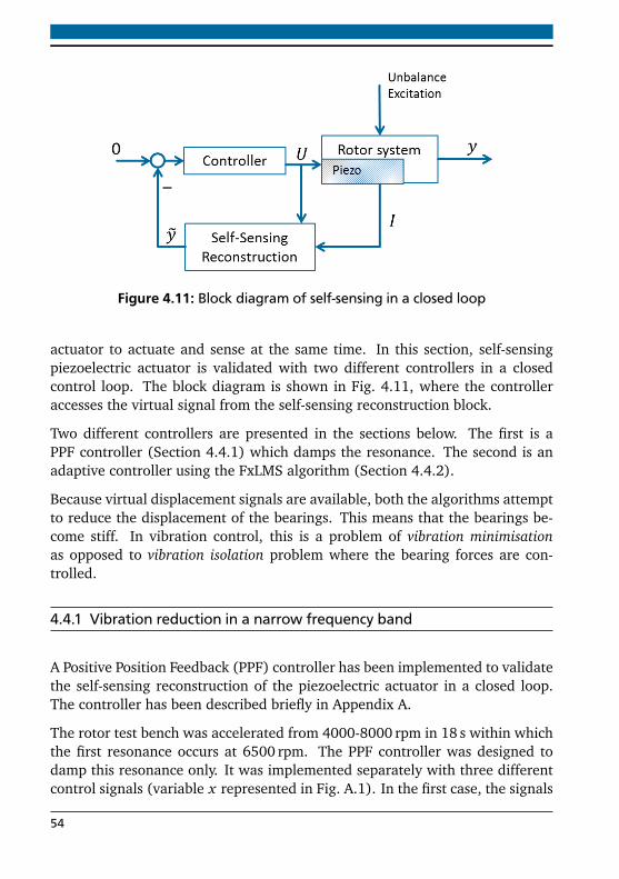
Figure 4.11: Block diagram of self-sensing in a closed loop

actuator to actuate and sense at the same time. In this section, self-sensingpiezoelectric actuator is validated with two different controllers in a closedcontrol loop. The block diagram is shown in Fig. 4.11, where the controlleraccesses the virtual signal from the self-sensing reconstruction block.

Two different controllers are presented in the sections below. The first is aPPF controller (Section 4.4.1) which damps the resonance. The second is anadaptive controller using the FxLMS algorithm (Section 4.4.2).

Because virtual displacement signals are available, both the algorithms attemptto reduce the displacement of the bearings. This means that the bearings be-come stiff. In vibration control, this is a problem of vibration minimisationas opposed to vibration isolation problem where the bearing forces are con-trolled.

4.4.1 Vibration reduction in a narrow frequency band

A Positive Position Feedback (PPF) controller has been implemented to validatethe self-sensing reconstruction of the piezoelectric actuator in a closed loop.The controller has been described briefly in Appendix A.

The rotor test bench was accelerated from 4000-8000 rpm in 18 s within whichthe first resonance occurs at 6500 rpm. The PPF controller was designed todamp this resonance only. It was implemented separately with three differentcontrol signals (variable x represented in Fig. A.1). In the first case, the signals

54

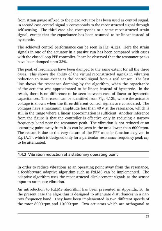
from strain gauge affixed to the piezo actuator has been used as control signal.In second case control signal x corresponds to the reconstructed signal throughself-sensing. The third case also corresponds to a same reconstructed strainsignal, except that the capacitance has been assumed to be linear instead ofhysteretic.

The achieved control performance can be seen in Fig. 4.12a. Here the strainsignals in one of the actuator in a passive run has been compared with caseswith the closed loop PPF controller. It can be observed that the resonance peakshave been damped upto 33%.

The peak of resonances have been damped to the same extent for all the threecases. This shows the ability of the virtual reconstructed signals in vibrationreduction to same extent as the control signal from a real sensor. The lastline shows the resonance damping by the algorithm, when the capacitanceof the actuator was approximated to be linear, instead of hysteretic. In theresult, there is no difference to be seen between case of linear or hystereticcapacitances. The reason can be identified from Fig. 4.12b, where the actuatorvoltage is shown when the three different control signals are considered. Thevoltages have a maximum amplitude less than 40 V at the resonance, which isstill in the range where a linear approximation is sufficient. Another inferencefrom the figure is that the controller is effective only in reducing a narrowfrequency band near the resonance peak. The vibration is not reduced at anoperating point away from it as can be seen in the area lower than 6000 rpm.The reason is due to the very nature of the PPF transfer function as given inEq. (A.1), which is designed only for a particular resonance frequency peakω fto be attenuated.

4.4.2 Vibration reduction at a stationary operating point

In order to reduce vibrations at an operating point away from the resonance,a feedforward adaptive algorithm such as FxLMS can be implemented. Theadaptive algorithm uses the reconstructed displacement signals as the sensorinput to attenuate vibration.

An introduction to FxLMS algorithm has been presented in Appendix B. Inthe present case the algorithm is designed to attenuate disturbances in a nar-row frequency band. They have been implemented in two different speeds ofthe rotor 8000 rpm and 10000 rpm. Two actuators which are orthogonal to

55

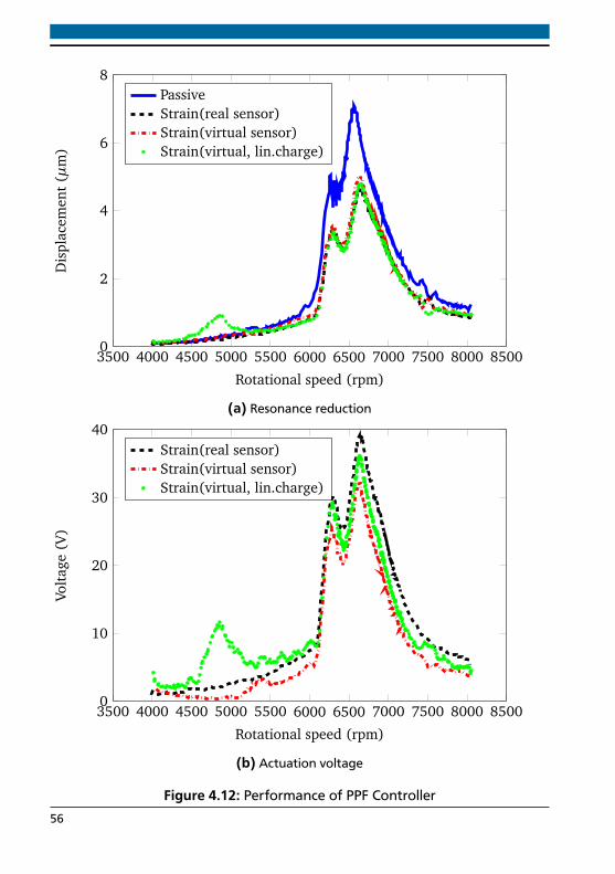
3500 4000 4500 5000 5500 6000 6500 7000 7500 8000 85000

2

4

6

8

Rotational speed (rpm)

Dis

plac

emen

t(µ

m)

PassiveStrain(real sensor)Strain(virtual sensor)Strain(virtual, lin.charge)

(a) Resonance reduction

3500 4000 4500 5000 5500 6000 6500 7000 7500 8000 85000

10

20

30

40

Rotational speed (rpm)

Volt

age

(V)

Strain(real sensor)Strain(virtual sensor)Strain(virtual, lin.charge)

(b) Actuation voltage

Figure 4.12: Performance of PPF Controller56

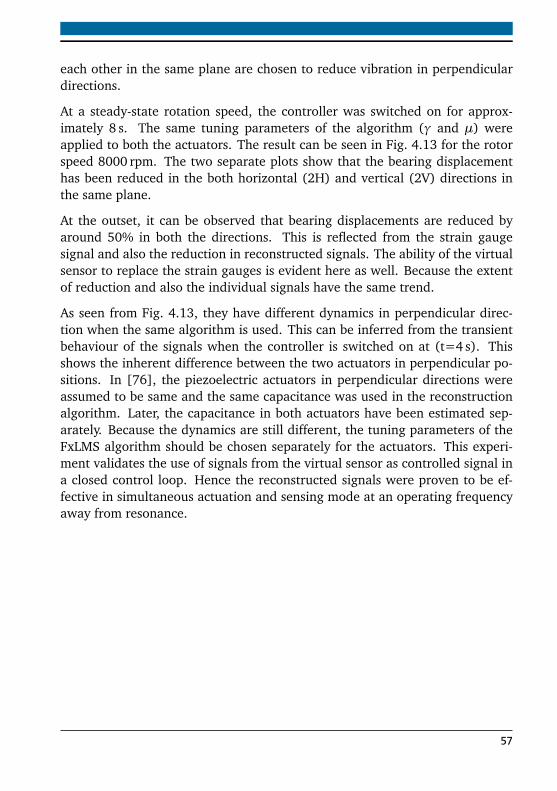
each other in the same plane are chosen to reduce vibration in perpendiculardirections.

At a steady-state rotation speed, the controller was switched on for approx-imately 8 s. The same tuning parameters of the algorithm (γ and µ) wereapplied to both the actuators. The result can be seen in Fig. 4.13 for the rotorspeed 8000 rpm. The two separate plots show that the bearing displacementhas been reduced in the both horizontal (2H) and vertical (2V) directions inthe same plane.

At the outset, it can be observed that bearing displacements are reduced byaround 50% in both the directions. This is reflected from the strain gaugesignal and also the reduction in reconstructed signals. The ability of the virtualsensor to replace the strain gauges is evident here as well. Because the extentof reduction and also the individual signals have the same trend.

As seen from Fig. 4.13, they have different dynamics in perpendicular direc-tion when the same algorithm is used. This can be inferred from the transientbehaviour of the signals when the controller is switched on at (t=4 s). Thisshows the inherent difference between the two actuators in perpendicular po-sitions. In [76], the piezoelectric actuators in perpendicular directions wereassumed to be same and the same capacitance was used in the reconstructionalgorithm. Later, the capacitance in both actuators have been estimated sep-arately. Because the dynamics are still different, the tuning parameters of theFxLMS algorithm should be chosen separately for the actuators. This experi-ment validates the use of signals from the virtual sensor as controlled signal ina closed control loop. Hence the reconstructed signals were proven to be ef-fective in simultaneous actuation and sensing mode at an operating frequencyaway from resonance.

57

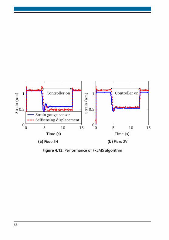
0 5 10 150

0.5

1

Time (s)

Stra

in(µ

m)

Strain gauge sensorSelfsensing displacement

Controller on

(a) Piezo 2H

0 5 10 150

0.5

1

Time (s)

Stra

in(µ

m) Controller on

(b) Piezo 2V

Figure 4.13: Performance of FxLMS algorithm

58

5 Fault detection in rotor systemsFault detection in machines can be performed either by signal-based or model-based methods. A signal-based method analyses the measured signal for spe-cific characteristics such as frequency, amplitudes and variances of signals,which are known as symptoms of faults. Some of the analysis methods in-clude correlation analysis, fourier analysis and ARMA models. Along withthese analytical symptoms, heuristical symptoms such as noise, colour, smelletc. can be included. Altogether error can be diagnosed with the help of error-symptom maps or by classification methods [77].

In a model-based method, the real system should be modelled mathematicallywith a good degree of accuracy. There are different methods to diagnose faultssuch as parity equations, parameter estimation techniques. The former methodis used for a stationary operating point or for additive faults. The latter methodis used for instationary operation or for multiplicative faults. A combinationof signal and model-based methods would lead to identification of a largernumber of faults in systems [57].

A possibility to extend the fault diagnosis to different fault types should beavailable. Because of this reason, the model-based method is opted for in thisresearch work. Rotational systems are characterised by gyroscopy which is arotational speed dependent phenomenon. In other words, rotor systems areLPV systems. Vibration surveys in real aircraft engine tests are carried outin quasi-static conditions, where the engine is accelerated very slowly. Henceparameter estimation techniques are applied to detect unbalance faults in rotorsystems.

5.1 Fault detection in time domain

From the basic equation of motion Eq. (3.10) of a mechanical system, the ac-celeration, velocity and displacements can be rewritten as Eq. (5.1). Here thegeneralised vectors (q, q and q) are to replaced by the translational DOF and

59

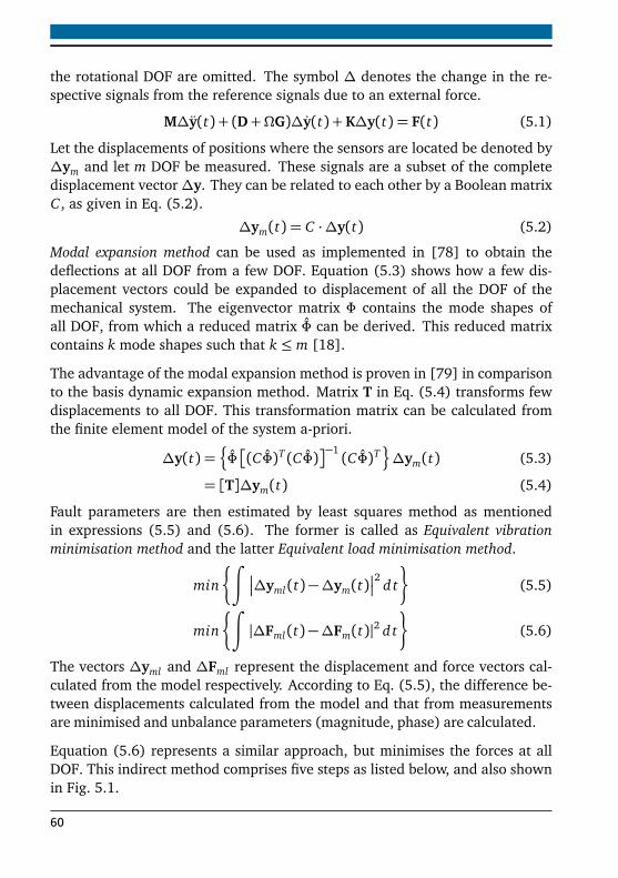
the rotational DOF are omitted. The symbol ∆ denotes the change in the re-spective signals from the reference signals due to an external force.

M∆y(t) + (D+ΩG)∆y(t) +K∆y(t) = F(t) (5.1)

Let the displacements of positions where the sensors are located be denoted by∆ym and let m DOF be measured. These signals are a subset of the completedisplacement vector∆y. They can be related to each other by a Boolean matrixC , as given in Eq. (5.2).

∆ym(t) = C ·∆y(t) (5.2)

Modal expansion method can be used as implemented in [78] to obtain thedeflections at all DOF from a few DOF. Equation (5.3) shows how a few dis-placement vectors could be expanded to displacement of all the DOF of themechanical system. The eigenvector matrix Φ contains the mode shapes ofall DOF, from which a reduced matrix Φ can be derived. This reduced matrixcontains k mode shapes such that k ≤ m [18].

The advantage of the modal expansion method is proven in [79] in comparisonto the basis dynamic expansion method. Matrix T in Eq. (5.4) transforms fewdisplacements to all DOF. This transformation matrix can be calculated fromthe finite element model of the system a-priori.

∆y(t) =¦

Φ

(CΦ)T (CΦ)−1(CΦ)T

©

∆ym(t) (5.3)

= [T]∆ym(t) (5.4)

Fault parameters are then estimated by least squares method as mentionedin expressions (5.5) and (5.6). The former is called as Equivalent vibrationminimisation method and the latter Equivalent load minimisation method.

min

∫

∆yml(t)−∆ym(t)

2d t

(5.5)

min

∫

|∆Fml(t)−∆Fm(t)|2 d t

(5.6)

The vectors ∆yml and ∆Fml represent the displacement and force vectors cal-culated from the model respectively. According to Eq. (5.5), the difference be-tween displacements calculated from the model and that from measurementsare minimised and unbalance parameters (magnitude, phase) are calculated.

Equation (5.6) represents a similar approach, but minimises the forces at allDOF. This indirect method comprises five steps as listed below, and also shownin Fig. 5.1.

60

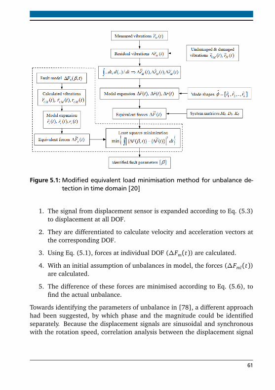
Figure 5.1: Modified equivalent load minimisation method for unbalance de-tection in time domain [20]

1. The signal from displacement sensor is expanded according to Eq. (5.3)to displacement at all DOF.

2. They are differentiated to calculate velocity and acceleration vectors atthe corresponding DOF.

3. Using Eq. (5.1), forces at individual DOF (∆Fm(t)) are calculated.

4. With an initial assumption of unbalances in model, the forces (∆Fml(t))are calculated.

5. The difference of these forces are minimised according to Eq. (5.6), tofind the actual unbalance.

Towards identifying the parameters of unbalance in [78], a different approachhad been suggested, by which phase and the magnitude could be identifiedseparately. Because the displacement signals are sinusoidal and synchronouswith the rotation speed, correlation analysis between the displacement signal

61

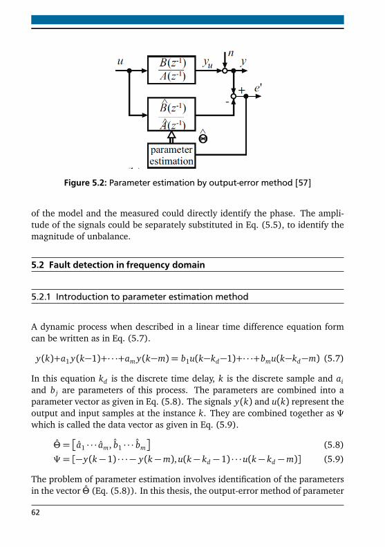
Figure 5.2: Parameter estimation by output-error method [57]

of the model and the measured could directly identify the phase. The ampli-tude of the signals could be separately substituted in Eq. (5.5), to identify themagnitude of unbalance.

5.2 Fault detection in frequency domain

5.2.1 Introduction to parameter estimation method

A dynamic process when described in a linear time difference equation formcan be written as in Eq. (5.7).

y(k)+a1 y(k−1)+· · ·+am y(k−m) = b1u(k−kd−1)+· · ·+bmu(k−kd−m) (5.7)

In this equation kd is the discrete time delay, k is the discrete sample and aiand b j are parameters of this process. The parameters are combined into aparameter vector as given in Eq. (5.8). The signals y(k) and u(k) represent theoutput and input samples at the instance k. They are combined together as Ψwhich is called the data vector as given in Eq. (5.9).

Θ =

a1 · · · am, b1 · · · bm

(5.8)

Ψ = [−y(k− 1) · · · − y(k−m), u(k− kd − 1) · · ·u(k− kd −m)] (5.9)

The problem of parameter estimation involves identification of the parametersin the vector Θ (Eq. (5.8)). In this thesis, the output-error method of parameter

62

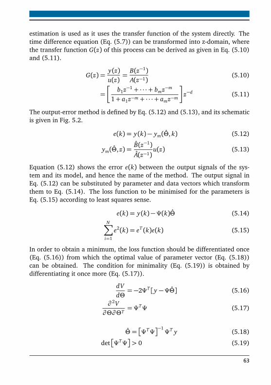
estimation is used as it uses the transfer function of the system directly. Thetime difference equation (Eq. (5.7)) can be transformed into z-domain, wherethe transfer function G(z) of this process can be derived as given in Eq. (5.10)and (5.11).

G(z) =y(z)u(z)

=B(z−1)A(z−1)

(5.10)

=

b1z−1 + · · ·+ bmz−m

1+ a1z−m + · · ·+ amz−m

z−d (5.11)

The output-error method is defined by Eq. (5.12) and (5.13), and its schematicis given in Fig. 5.2.

e(k) = y(k)− ym(Θ, k) (5.12)

ym(Θ, z) =B(z−1)A(z−1)

u(z) (5.13)

Equation (5.12) shows the error e(k) between the output signals of the sys-tem and its model, and hence the name of the method. The output signal inEq. (5.12) can be substituted by parameter and data vectors which transformthem to Eq. (5.14). The loss function to be minimised for the parameters isEq. (5.15) according to least squares sense.

e(k) = y(k)−Ψ(k)Θ (5.14)N∑

i=1

e2(k) = eT (k)e(k) (5.15)

In order to obtain a minimum, the loss function should be differentiated once(Eq. (5.16)) from which the optimal value of parameter vector (Eq. (5.18))can be obtained. The condition for minimality (Eq. (5.19)) is obtained bydifferentiating it once more (Eq. (5.17)).

dVdΘ= −2ΨT [y −ΨΘ] (5.16)

∂ 2V∂Θ∂ΘT

= ΨTΨ (5.17)

Θ =

ΨTΨ−1ΨT y (5.18)

det

ΨTΨ

> 0 (5.19)

63

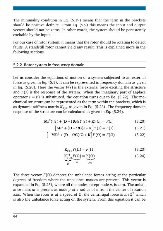
The minimality condition in Eq. (5.19) means that the term in the bracketsshould be positive definite. From Eq. (5.9) this means the input and outputvectors should not be zeros. In other words, the system should be persistentlyexcitable by the input.

For our case of rotor system, it means that the rotor should be rotating to detectfaults. A standstill rotor cannot yield any result. This is explained more in thefollowing sections.

5.2.2 Rotor system in frequency domain

Let us consider the equations of motion of a system subjected to an externalforce as given in Eq. (5.1). It can be represented in frequency domain as givenin Eq. (5.20). Here the vector F(s) is the external force exciting the structureand Y (s) is the response of the system. When the imaginary part of Laplaceoperator s = iΩ is substituted, the equation turns out to Eq. (5.22). The me-chanical structure can be represented as the term within the brackets, which isas dynamic stiffness matrix Kd yn as given in Eq. (5.23). The frequency domainresponse of the structure can be calculated as given in Eq. (5.24).

Ms2Y (s) + (D+ΩG)sY (s) +KY (s) = F(s) (5.20)

Ms2 + (D+ΩG)s+K

Y (s) = F(s) (5.21)

−MΩ2 + (D+ΩG)iΩ+K

Y (Ω) = F(Ω) (5.22)

Kd ynY (Ω) = F(Ω) (5.23)

K−1d yn︸︷︷︸

Θ

F(Ω)︸︷︷︸

Ψ

= Y (Ω)︸︷︷︸

ym

(5.24)

The force vector F(Ω) denotes the unbalance forces acting at the particulardegrees of freedom where the unbalance masses are present. This vector isexpanded in Eq. (5.25), where all the nodes except node p, is zero. The unbal-ance mass m is present at node p at a radius of ε from the center of rotationaxis. When the rotor is at a speed of Ω, the centrifugal force is mεΩ2 whichis also the unbalance force acting on the system. From this equation it can be

64

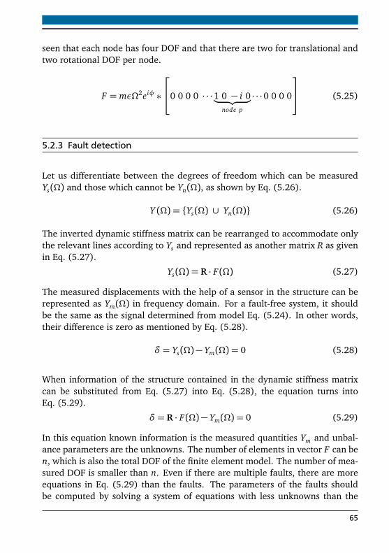
seen that each node has four DOF and that there are two for translational andtwo rotational DOF per node.

F = mεΩ2eiφ ∗

0 0 0 0 · · ·1 0 − i 0︸ ︷︷ ︸

node p

· · ·0 0 0 0

(5.25)

5.2.3 Fault detection

Let us differentiate between the degrees of freedom which can be measuredYs(Ω) and those which cannot be Yn(Ω), as shown by Eq. (5.26).

Y (Ω) = Ys(Ω) ∪ Yn(Ω) (5.26)

The inverted dynamic stiffness matrix can be rearranged to accommodate onlythe relevant lines according to Ys and represented as another matrix R as givenin Eq. (5.27).

Ys(Ω) = R · F(Ω) (5.27)

The measured displacements with the help of a sensor in the structure can berepresented as Ym(Ω) in frequency domain. For a fault-free system, it shouldbe the same as the signal determined from model Eq. (5.24). In other words,their difference is zero as mentioned by Eq. (5.28).

δ = Ys(Ω)− Ym(Ω) = 0 (5.28)

When information of the structure contained in the dynamic stiffness matrixcan be substituted from Eq. (5.27) into Eq. (5.28), the equation turns intoEq. (5.29).

δ = R · F(Ω)− Ym(Ω) = 0 (5.29)

In this equation known information is the measured quantities Ym and unbal-ance parameters are the unknowns. The number of elements in vector F can ben, which is also the total DOF of the finite element model. The number of mea-sured DOF is smaller than n. Even if there are multiple faults, there are moreequations in Eq. (5.29) than the faults. The parameters of the faults shouldbe computed by solving a system of equations with less unknowns than the

65

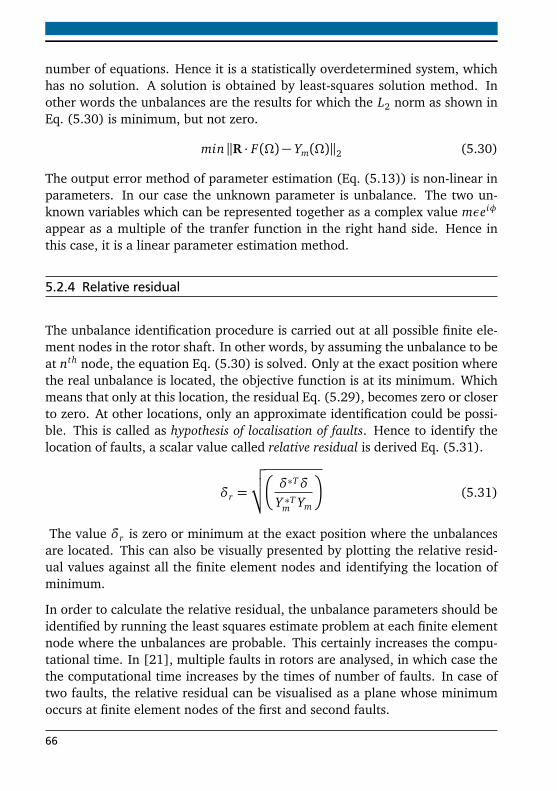
number of equations. Hence it is a statistically overdetermined system, whichhas no solution. A solution is obtained by least-squares solution method. Inother words the unbalances are the results for which the L2 norm as shown inEq. (5.30) is minimum, but not zero.

min‖R · F(Ω)− Ym(Ω)‖2 (5.30)

The output error method of parameter estimation (Eq. (5.13)) is non-linear inparameters. In our case the unknown parameter is unbalance. The two un-known variables which can be represented together as a complex value mεeiφ

appear as a multiple of the tranfer function in the right hand side. Hence inthis case, it is a linear parameter estimation method.

5.2.4 Relative residual

The unbalance identification procedure is carried out at all possible finite ele-ment nodes in the rotor shaft. In other words, by assuming the unbalance to beat nth node, the equation Eq. (5.30) is solved. Only at the exact position wherethe real unbalance is located, the objective function is at its minimum. Whichmeans that only at this location, the residual Eq. (5.29), becomes zero or closerto zero. At other locations, only an approximate identification could be possi-ble. This is called as hypothesis of localisation of faults. Hence to identify thelocation of faults, a scalar value called relative residual is derived Eq. (5.31).

δr =

√

√

√

δ∗Tδ

Y ∗Tm Ym

(5.31)

The value δr is zero or minimum at the exact position where the unbalancesare located. This can also be visually presented by plotting the relative resid-ual values against all the finite element nodes and identifying the location ofminimum.

In order to calculate the relative residual, the unbalance parameters should beidentified by running the least squares estimate problem at each finite elementnode where the unbalances are probable. This certainly increases the compu-tational time. In [21], multiple faults in rotors are analysed, in which case thethe computational time increases by the times of number of faults. In case oftwo faults, the relative residual can be visualised as a plane whose minimumoccurs at finite element nodes of the first and second faults.

66

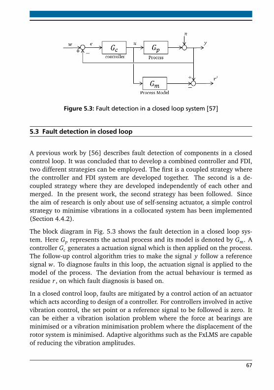
Figure 5.3: Fault detection in a closed loop system [57]

5.3 Fault detection in closed loop

A previous work by [56] describes fault detection of components in a closedcontrol loop. It was concluded that to develop a combined controller and FDI,two different strategies can be employed. The first is a coupled strategy wherethe controller and FDI system are developed together. The second is a de-coupled strategy where they are developed independently of each other andmerged. In the present work, the second strategy has been followed. Sincethe aim of research is only about use of self-sensing actuator, a simple controlstrategy to minimise vibrations in a collocated system has been implemented(Section 4.4.2).

The block diagram in Fig. 5.3 shows the fault detection in a closed loop sys-tem. Here Gp represents the actual process and its model is denoted by Gm. Acontroller Gc generates a actuation signal which is then applied on the process.The follow-up control algorithm tries to make the signal y follow a referencesignal w. To diagnose faults in this loop, the actuation signal is applied to themodel of the process. The deviation from the actual behaviour is termed asresidue r, on which fault diagnosis is based on.

In a closed control loop, faults are mitigated by a control action of an actuatorwhich acts according to design of a controller. For controllers involved in activevibration control, the set point or a reference signal to be followed is zero. Itcan be either a vibration isolation problem where the force at bearings areminimised or a vibration minimisation problem where the displacement of therotor system is minimised. Adaptive algorithms such as the FxLMS are capableof reducing the vibration amplitudes.

67

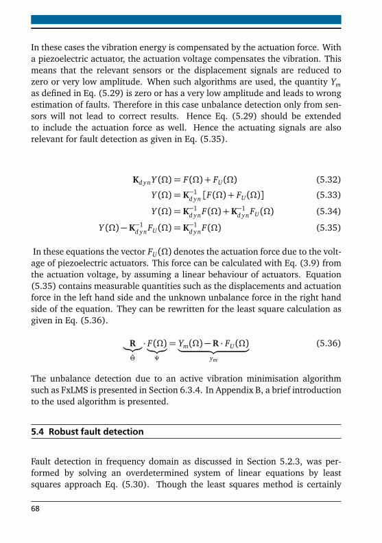
In these cases the vibration energy is compensated by the actuation force. Witha piezoelectric actuator, the actuation voltage compensates the vibration. Thismeans that the relevant sensors or the displacement signals are reduced tozero or very low amplitude. When such algorithms are used, the quantity Ymas defined in Eq. (5.29) is zero or has a very low amplitude and leads to wrongestimation of faults. Therefore in this case unbalance detection only from sen-sors will not lead to correct results. Hence Eq. (5.29) should be extendedto include the actuation force as well. Hence the actuating signals are alsorelevant for fault detection as given in Eq. (5.35).

Kd ynY (Ω) = F(Ω) + FU(Ω) (5.32)

Y (Ω) = K−1d yn [F(Ω) + FU(Ω)] (5.33)

Y (Ω) = K−1d ynF(Ω) +K−1

d ynFU(Ω) (5.34)

Y (Ω)−K−1d ynFU(Ω) = K−1

d ynF(Ω) (5.35)

In these equations the vector FU(Ω) denotes the actuation force due to the volt-age of piezoelectric actuators. This force can be calculated with Eq. (3.9) fromthe actuation voltage, by assuming a linear behaviour of actuators. Equation(5.35) contains measurable quantities such as the displacements and actuationforce in the left hand side and the unknown unbalance force in the right handside of the equation. They can be rewritten for the least square calculation asgiven in Eq. (5.36).

R︸︷︷︸

Θ

· F(Ω)︸︷︷︸

Ψ

= Ym(Ω)−R · FU(Ω)︸ ︷︷ ︸

ym

(5.36)

The unbalance detection due to an active vibration minimisation algorithmsuch as FxLMS is presented in Section 6.3.4. In Appendix B, a brief introductionto the used algorithm is presented.

5.4 Robust fault detection

Fault detection in frequency domain as discussed in Section 5.2.3, was per-formed by solving an overdetermined system of linear equations by leastsquares approach Eq. (5.30). Though the least squares method is certainly

68

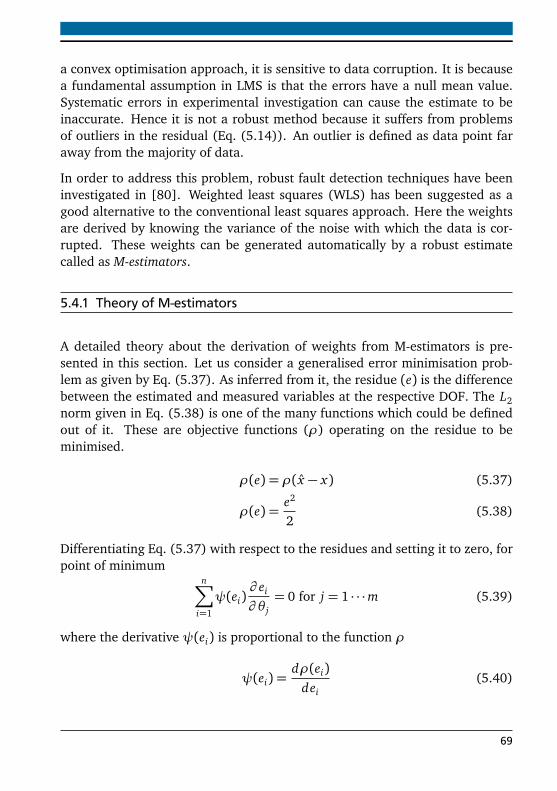
a convex optimisation approach, it is sensitive to data corruption. It is becausea fundamental assumption in LMS is that the errors have a null mean value.Systematic errors in experimental investigation can cause the estimate to beinaccurate. Hence it is not a robust method because it suffers from problemsof outliers in the residual (Eq. (5.14)). An outlier is defined as data point faraway from the majority of data.

In order to address this problem, robust fault detection techniques have beeninvestigated in [80]. Weighted least squares (WLS) has been suggested as agood alternative to the conventional least squares approach. Here the weightsare derived by knowing the variance of the noise with which the data is cor-rupted. These weights can be generated automatically by a robust estimatecalled as M-estimators.

5.4.1 Theory of M-estimators

A detailed theory about the derivation of weights from M-estimators is pre-sented in this section. Let us consider a generalised error minimisation prob-lem as given by Eq. (5.37). As inferred from it, the residue (e) is the differencebetween the estimated and measured variables at the respective DOF. The L2norm given in Eq. (5.38) is one of the many functions which could be definedout of it. These are objective functions (ρ) operating on the residue to beminimised.

ρ(e) = ρ( x − x) (5.37)

ρ(e) =e2

2(5.38)

Differentiating Eq. (5.37) with respect to the residues and setting it to zero, forpoint of minimum

n∑

i=1

ψ(ei)∂ ei

∂ θ j= 0 for j = 1 · · ·m (5.39)

where the derivative ψ(ei) is proportional to the function ρ

ψ(ei) =dρ(ei)

dei(5.40)

69

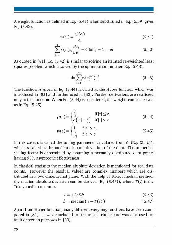
A weight function as defined in Eq. (5.41) when substituted in Eq. (5.39) givesEq. (5.42).

w(ei) =ψ(ei)

ei(5.41)

n∑

i=1

w(ei)ei∂ ei

∂ θ j= 0 for j = 1 · · ·m (5.42)

As quoted in [81], Eq. (5.42) is similar to solving an iterated re-weighted leastsquares problem which is solved by the optimisation function Eq. (5.43).

minn∑

i=1

w(et−1i )e2

i (5.43)

The function as given in Eq. (5.44) is called as the Huber function which wasintroduced in [82] and further used in [83]. Further derivations are restrictedonly to this function. When Eq. (5.44) is considered, the weights can be derivedas in Eq. (5.45).

ρ(e) =

¨

e2

2 if |e| ≤ c,

c

|e| − c2

if |e|> c(5.44)

w(e) =

¨

1 if |e| ≤ c,c|e| if |e|> c

(5.45)

In this case, c is called the tuning parameter calculated from σ (Eq. (5.46)),which is called as the median absolute deviation of the data. The numericalscaling factor is determined by assuming a normally distributed data pointshaving 95% asymptotic effectiveness.

In classical statistics the median absolute deviation is mentioned for real datapoints. However the residual values are complex numbers which are dis-tributed in a two dimensional plane. With the help of Tukeys median method,the median absolute deviation can be derived (Eq. (5.47)), where T (.) is theTukey median operator.

c = 1.345σ (5.46)

σ =median (|e− T (e)|) (5.47)

Apart from Huber function, many different weighing functions have been com-pared in [81]. It was concluded to be the best choice and was also used forfault detection purposes in [80].

70

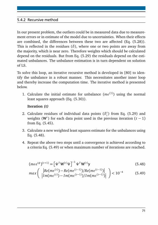
5.4.2 Recursive method

In our present problem, the outliers could be in measured data due to measure-ment errors or in estimate of the model due to uncertainties. When their effectsare combined, the differences between these two are affected (Eq. (5.28)).This is reflected in the residues (δ), where one or two points are away fromthe majority, which is near zero. Therefore weights which should be calculateddepend on the residuals. But from Eq. (5.29) the residuals depend on the esti-mated unbalances. The unbalance estimation is in turn dependent on solutionof LS.

To solve this loop, an iterative recursive method is developed in [80] to iden-tify the unbalance in a robust manner. This necessitates another inner loopand thereby increase the computation time. The iterative method is presentedbelow.

1. Calculate the initial estimate for unbalance (mε(1)) using the normalleast squares approach (Eq. (5.30)).

Iteration (t)

2. Calculate residues of individual data points (δti ) from Eq. (5.29) and

weights (Wt) for each data point used in the previous iteration (t − 1)from Eq. (5.45).

3. Calculate a new weighted least squares estimate for the unbalances usingEq. (5.48).

4. Repeat the above two steps until a convergence is achieved according toa criteria Eq. (5.49) or when maximum number of iterations are reached.

(mεeiφ)(t+1) =

ΨT W(t)Ψ−1ΨT W(t)y (5.48)

max

Re(mε(t))− Re(mε(t−1))/Re(mε(t−1))

Im(mε(t))− Im(mε(t−1))/Im(mε(t−1))

< 10−4 (5.49)

71

6 Results and discussionThe individual systems presented in the preceding chapters (3-5) are put to-gether in this chapter and results are derived. Faults are detected with thehelp of bearing displacements at the respective rotor systems. Instead of sepa-rate displacement sensors, signals from actuators which are placed in bearingscan be used to derive their displacement. Apart from magnitude and phase ofunbalances, their position were determined with the help of relative residualpresented in 5.2.4.

This chapter is ordered in the following way. In Sections 6.1, 6.2 results fromsimulations using model of the rotor system at IMS are presented. This isfollowed by unbalances diagnosed with data measured from the test bench inSection 6.3. Unbalance detected from virtual strain signals are compared fromthose obtained from real strain gauge signals. Apart from stationary tests,quasi-static and simultaneous actuation and sensing cases are also tested.

Subsequently in Section 6.4, the high pressure rotor model of an aircraft engineis analysed with its three different actuator configurations.

At the end, all the results are discussed and conclusions derived. Out of allthe results, a good unbalance detection is considered when the relative errorin magnitude is within ±25% and when the absolute phase deviation is within±45.

6.1 Fault detection in time domain

Fault detection was simulated with a model of the test bench rotor in MAT-LAB. In this simulation, the model of the system is compared against the samemodel for faults. The signals representing those measured from sensors arecorrupted with band limited noise to emulate conditions of disturbances inreal measurements.

As seen in Tab. 6.1, unbalances were detected in stationary operating pointsboth in simulation and in test bench. In simulations, the unbalance magnitude

73

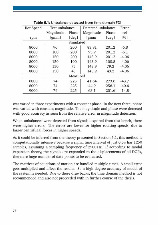
Table 6.1: Unbalance detected from time domain FDIRot.Speed Test unbalance Detected unbalance Error

Magnitude Phase Magnitude Phase relrpm [gmm] [deg] [gmm] [deg] [%]

Simulated8000 90 200 83.91 201.2 -6.88000 100 200 93.9 201.2 -6.18000 150 200 143.9 201.2 -4.068000 150 100 143.9 100.8 -4.068000 150 75 143.9 79.2 -4.068000 150 45 143.9 43.2 -4.06

Measured6000 74 225 41.64 273.6 -43.78000 74 225 44.9 256.1 -40.69000 74 225 63.1 201.6 -14.8

was varied in three experiments with a constant phase. In the next three, phasewas varied with constant magnitude. The magnitude and phase were detectedwith good accuracy as seen from the relative error in magnitude detection.

When unbalances were detected from signals acquired from test bench, therewere higher errors. The errors are lower for higher rotating speeds, due tolarger centrifugal forces in higher speeds.

As it could be inferred from the theory presented in Section 5.1, this method iscomputationally intensive because a signal time interval of just 0.5 s has 1250samples, assuming a sampling frequency of 2500 Hz. If according to modalexpansion theory, the signals are expanded to the displacements of all DOFs,there are huge number of data points to be evaluated.

The matrices of equations of motion are handled multiple times. A small errorgets multiplied and affect the results. So a high degree accuracy of model ofthe system is needed. Due to these drawbacks, the time domain method is notrecommended and also not proceeded with in further course of the thesis.

74

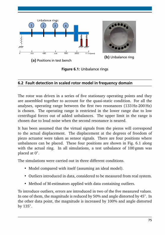
(a) Positions in test bench(b) Unbalance ring

Figure 6.1: Unbalance rings

6.2 Fault detection in scaled rotor model in frequency domain

The rotor was driven in a series of five stationary operating points and theyare assembled together to account for the quasi-static condition. For all theanalyses, operating range between the first two resonances (133 Hz-200 Hz)is chosen. The operating range is restricted in the lower range due to lowcentrifugal forces out of added unbalances. The upper limit in the range ischosen due to loud noise when the second resonance is neared.

It has been assumed that the virtual signals from the piezos will correspondto the actual displacement. The displacement at the degrees of freedom ofpiezo actuator were taken as sensor signals. There are four positions whereunbalances can be placed. These four positions are shown in Fig. 6.1 alongwith the actual ring. In all simulations, a test unbalance of 100 gmm wasplaced at 0.

The simulations were carried out in three different conditions.

• Model compared with itself (assuming an ideal model).

• Outliers introduced in data, considered to be measured from real system.

• Method of M-estimators applied with data containing outliers.

To introduce outliers, errors are introduced in two of the five measured values.In one of them, the magnitude is reduced by 50% and angle distorted by 45. Inthe other data point, the magnitude is increased by 100% and angle distortedby 135.

75

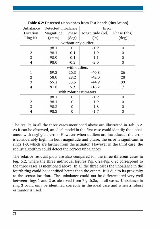
Table 6.2: Detected unbalances from Test bench (simulation)Unbalance Detected unbalance ErrorLocation Magnitude Phase Magnitude (rel) Phase (abs)Ring Nr. (gmm) (deg) (%) (deg)

without any outlier1 98.1 0 -1.9 02 98.1 -0.1 -1.9 03 98.9 -0.1 -1.1 04 98.0 -0.2 -2.0 0

with outliers1 59.2 26.3 -40.8 262 58.0 28.2 -42.0 283 55.1 33.5 -44.9 334 81.8 6.9 -18.2 7

with robust estimators1 98.1 0 -1.9 02 98.1 0 -1.9 03 98.2 0 -1.8 04 98.3 0 -1.7 0

The results in all the three cases mentioned above are illustrated in Tab. 6.2.As it can be observed, an ideal model in the first case could identify the unbal-ances with negligible error. However when outliers are introduced, the erroris considerably high. In both magnitude and phase, the error is significant inrings 1-3, which are farther from the actuator. However in the third case, therobust algorithm could detect the correct unbalances.

The relative residual plots are also compared for the three different cases inFig. 6.2, where the three individual figures Fig. 6.2a-Fig. 6.2c correspond tothe three cases as mentioned above. In all the three cases the unbalance in thefourth ring could be identified better than the others. It is due to its proximityto the sensor location. The unbalance could not be differentiated very wellbetween rings 1 and 2 as observed from Fig. 6.2a, in all cases. Unbalance inring 3 could only be identified correctly in the ideal case and when a robustestimator is used.

76

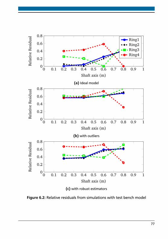
0 0.1 0.2 0.3 0.4 0.5 0.6 0.7 0.8 0.9 10

0.2

0.4

0.6

0.8

Shaft axis (m)

Rel

ativ

eR

esid

ual

Ring1Ring2Ring3Ring4

(a) Ideal model

0 0.1 0.2 0.3 0.4 0.5 0.6 0.7 0.8 0.9 10

0.2

0.4

0.6

0.8

Shaft axis (m)

Rel

ativ

eR

esid

ual

(b) with outliers

0 0.1 0.2 0.3 0.4 0.5 0.6 0.7 0.8 0.9 10

0.2

0.4

0.6

0.8

Shaft axis (m)

Rel

ativ

eR

esid

ual

(c) with robust estimators

Figure 6.2: Relative residuals from simulations with test bench model

77

6.3 Fault detection using measured signals from test bench

Unbalance detection method was also tested on the available test bench. Un-balances of three different magnitudes 57 gmm, 74 gmm and 103 gmm areplaced alternatively in each unbalance ring at different angular positions.They were mounted in subsequent tests, with all the test cases mentioned inTab. 6.3.

A reference measurement was initially made after which test unbalances werescrewed to the unbalance rings according to individual test cases. The mea-sured sensor signals are subtracted from the respective reference signals at thecorresponding operating points. Because the unbalance is sensitive to phasesas well, it is necessary to measure the angular position of the shaft with thehelp of an encoder. The measured signals were processed before used for un-balance detection. They were windowed (rectangular window) whose samplelength was 1250 samples or in other words 0.5 s in a sampling frequency of2500 Hz. The windows always start at the sample where the encoder value is0.

There were test cases where the vibrations were too high to cross the first res-onance at 109 Hz. In such cases, PPF controller presented in Section 4.4.1 wasswitched on, to damp the resonance peak and then turned off while acquiringthe data after crossing the resonance.

Various tests were performed such as running at series of stationary operatingpoints, quasi-static run, simultaneous actuation and sensing in a closed loop.The results of individual tests are presented below.

6.3.1 Analysis at stationary operating points

As a first test, the rotor was driven in five operating points in a stationarycondition (8000 rpm-12000 rpm in steps of 1000 rpm). Sensor signals wererecorded at steady state conditions in each operating point for each of the testcases mentioned in Tab. 6.3. Unbalance detection was carried out by accumu-lating the sensor signals for all the operating points driven in a particular testcase.

Because they are real measurements, no separate model disturbances ornoise superposition or signal distortion were included. The results obtained

78

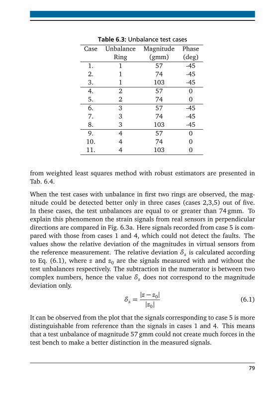
Table 6.3: Unbalance test casesCase Unbalance Magnitude Phase

Ring (gmm) (deg)1. 1 57 -452. 1 74 -453. 1 103 -454. 2 57 05. 2 74 06. 3 57 -457. 3 74 -458. 3 103 -459. 4 57 0

10. 4 74 011. 4 103 0

from weighted least squares method with robust estimators are presented inTab. 6.4.

When the test cases with unbalance in first two rings are observed, the mag-nitude could be detected better only in three cases (cases 2,3,5) out of five.In these cases, the test unbalances are equal to or greater than 74 gmm. Toexplain this phenomenon the strain signals from real sensors in perpendiculardirections are compared in Fig. 6.3a. Here signals recorded from case 5 is com-pared with those from cases 1 and 4, which could not detect the faults. Thevalues show the relative deviation of the magnitudes in virtual sensors fromthe reference measurement. The relative deviation δz is calculated accordingto Eq. (6.1), where z and z0 are the signals measured with and without thetest unbalances respectively. The subtraction in the numerator is between twocomplex numbers, hence the value δz does not correspond to the magnitudedeviation only.

δz =|z − z0||z0|

(6.1)

It can be observed from the plot that the signals corresponding to case 5 is moredistinguishable from reference than the signals in cases 1 and 4. This meansthat a test unbalance of magnitude 57 gmm could not create much forces in thetest bench to make a better distinction in the measured signals.

79

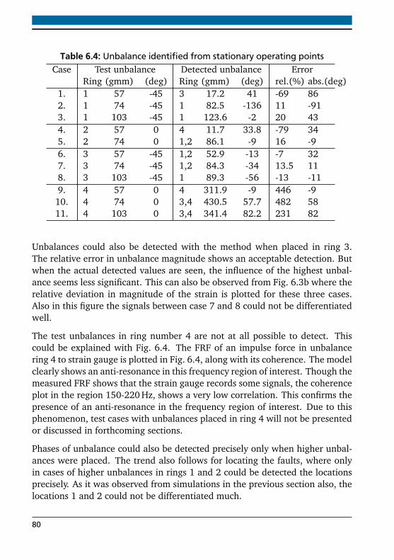
Table 6.4: Unbalance identified from stationary operating pointsCase Test unbalance Detected unbalance Error

Ring (gmm) (deg) Ring (gmm) (deg) rel.(%) abs.(deg)1. 1 57 -45 3 17.2 41 -69 862. 1 74 -45 1 82.5 -136 11 -913. 1 103 -45 1 123.6 -2 20 434. 2 57 0 4 11.7 33.8 -79 345. 2 74 0 1,2 86.1 -9 16 -96. 3 57 -45 1,2 52.9 -13 -7 327. 3 74 -45 1,2 84.3 -34 13.5 118. 3 103 -45 1 89.3 -56 -13 -119. 4 57 0 4 311.9 -9 446 -9

10. 4 74 0 3,4 430.5 57.7 482 5811. 4 103 0 3,4 341.4 82.2 231 82

Unbalances could also be detected with the method when placed in ring 3.The relative error in unbalance magnitude shows an acceptable detection. Butwhen the actual detected values are seen, the influence of the highest unbal-ance seems less significant. This can also be observed from Fig. 6.3b where therelative deviation in magnitude of the strain is plotted for these three cases.Also in this figure the signals between case 7 and 8 could not be differentiatedwell.

The test unbalances in ring number 4 are not at all possible to detect. Thiscould be explained with Fig. 6.4. The FRF of an impulse force in unbalancering 4 to strain gauge is plotted in Fig. 6.4, along with its coherence. The modelclearly shows an anti-resonance in this frequency region of interest. Though themeasured FRF shows that the strain gauge records some signals, the coherenceplot in the region 150-220 Hz, shows a very low correlation. This confirms thepresence of an anti-resonance in the frequency region of interest. Due to thisphenomenon, test cases with unbalances placed in ring 4 will not be presentedor discussed in forthcoming sections.

Phases of unbalance could also be detected precisely only when higher unbal-ances were placed. The trend also follows for locating the faults, where onlyin cases of higher unbalances in rings 1 and 2 could be detected the locationsprecisely. As it was observed from simulations in the previous section also, thelocations 1 and 2 could not be differentiated much.

80

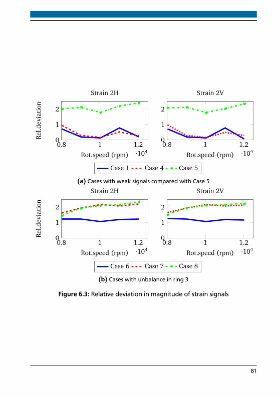
0.8 1 1.2·104

0

1

2

Rot.speed (rpm)

Rel

.dev

iati

on

Strain 2H

Case 1 Case 4 Case 5

0.8 1 1.2·104

0

1

2

Rot.speed (rpm)

Strain 2V

(a) Cases with weak signals compared with Case 5

0.8 1 1.2·104

0

1

2

Rot.speed (rpm)

Rel

.dev

iati

on

Strain 2H

Case 6 Case 7 Case 8

0.8 1 1.2·104

0

1

2

Rot.speed (rpm)

Strain 2V

(b) Cases with unbalance in ring 3

Figure 6.3: Relative deviation in magnitude of strain signals

81

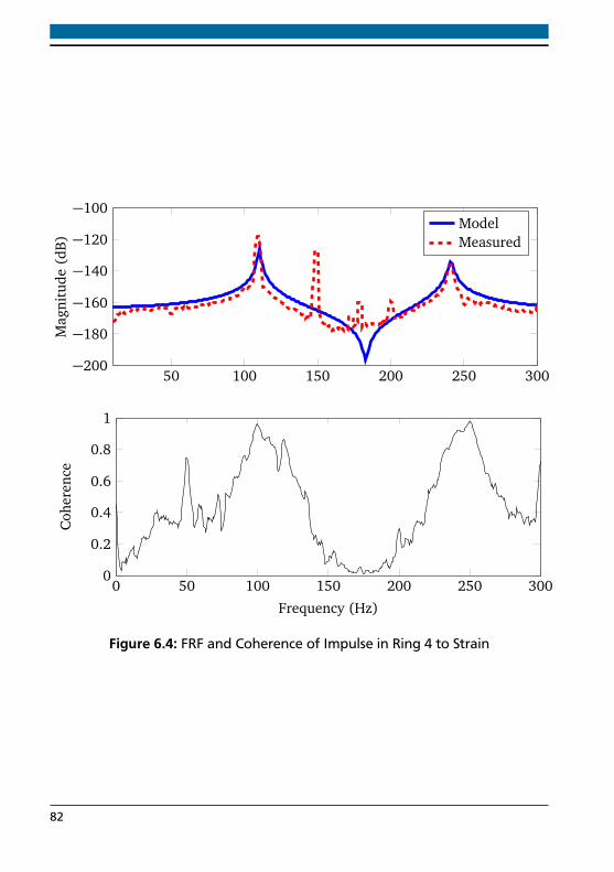
50 100 150 200 250 300−200

−180

−160

−140

−120

−100

Mag

nitu

de(d

B)

ModelMeasured

0 50 100 150 200 250 3000

0.2

0.4

0.6

0.8

1

Frequency (Hz)

Coh

eren

ce

Figure 6.4: FRF and Coherence of Impulse in Ring 4 to Strain

82

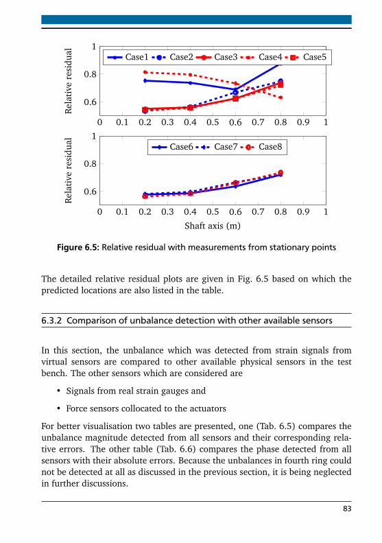
0 0.1 0.2 0.3 0.4 0.5 0.6 0.7 0.8 0.9 1

0.6

0.8

1

Rel

ativ

ere

sidu

al Case1 Case2 Case3 Case4 Case5

0 0.1 0.2 0.3 0.4 0.5 0.6 0.7 0.8 0.9 1

0.6

0.8

1

Shaft axis (m)

Rel

ativ

ere

sidu

al Case6 Case7 Case8

Figure 6.5: Relative residual with measurements from stationary points

The detailed relative residual plots are given in Fig. 6.5 based on which thepredicted locations are also listed in the table.

6.3.2 Comparison of unbalance detection with other available sensors

In this section, the unbalance which was detected from strain signals fromvirtual sensors are compared to other available physical sensors in the testbench. The other sensors which are considered are

• Signals from real strain gauges and

• Force sensors collocated to the actuators

For better visualisation two tables are presented, one (Tab. 6.5) compares theunbalance magnitude detected from all sensors and their corresponding rela-tive errors. The other table (Tab. 6.6) compares the phase detected from allsensors with their absolute errors. Because the unbalances in fourth ring couldnot be detected at all as discussed in the previous section, it is being neglectedin further discussions.

83

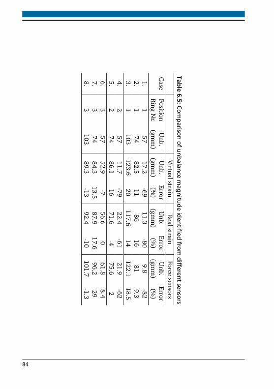
Table6.5:Com

parisonofunbalance

magnitude

identifiedfrom

differentsensors

VirtualstrainR

ealstrainForce

sensorsC

asePosition

Unb.

Unb.

ErrorU

nb.Error

Unb.

ErrorR

ingN

r.(gm

m)

(gmm

)(%

)(gm

m)

(%)

(gmm

)(%

)1.

157

17.2-69

11.3-80

9.8-82

2.1

7482.5

1186

1681

9.33.

1103

123.620

117.614

122.118.5

4.2

5711.7

-7922.4

-6121.9

-625.

274

86.116

71.6-4

75.62

6.3

5752.9

-756.6

061.8

8.47.

374

84.313.5

87.917.6

96.229

8.3

10389.3

-1392.4

-10101.7

-1.3

84

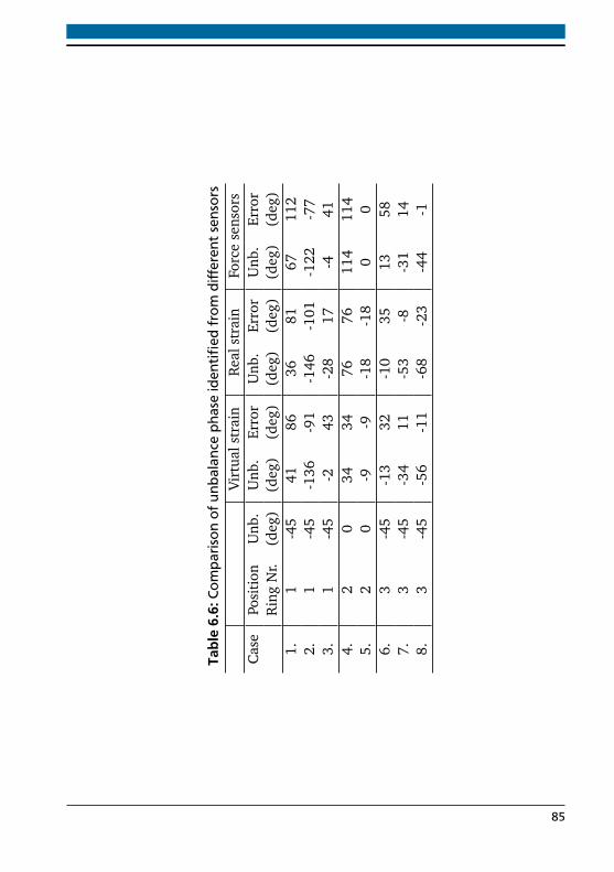
Table6.6:

Com

paris

onof

unba

lanc

eph

ase

iden

tified

from

diff

eren

tsen

sors

Virt

uals

trai

nR

eals

trai

nFo

rce

sens

ors

Cas

ePo

siti

onU

nb.

Unb

.Er

ror

Unb

.Er

ror

Unb

.Er

ror

Rin

gN

r.(d

eg)

(deg

)(d

eg)

(deg

)(d

eg)

(deg

)(d

eg)

1.1

-45

4186

3681

6711

22.

1-4

5-1

36-9

1-1

46-1

01-1

22-7

73.

1-4

5-2

43-2

817

-441

4.2

034

3476

7611

411

45.

20

-9-9

-18

-18

00

6.3

-45

-13

32-1

035

1358

7.3

-45

-34

11-5

3-8

-31

148.

3-4

5-5

6-1

1-6

8-2

3-4

4-1

85

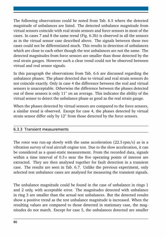
The following observations could be noted from Tab. 6.5 where the detectedmagnitude of unbalances are listed. The detected unbalance magnitude fromvirtual sensors coincide with real strain sensors and force sensors in most of thecases. In cases 7 and 8 the same trend (Fig. 6.3b) is observed in all the sensorsas in the virtual sensor case described above. The signals between these twocases could not be differentiated much. This results in detection of unbalanceswhich are close to each other though the test unbalances are not the same. Thedetected magnitudes from force sensors are smaller than those detected by thereal strain gauges. However such a clear trend could not be observed betweenvirtual and real sensor signals.

In this paragraph the observations from Tab. 6.6 are discussed regarding theunbalance phases. The phase detected due to virtual and real strain sensors donot coincide exactly. Only in case 4 the difference between the real and virtualsensors is unacceptable. Otherwise the difference between the phases detectedout of these sensors is only 11 on an average. This indicates the ability of thevirtual sensor to detect the unbalance phase as good as the real strain gauge.

When the phases detected by virtual sensors are compared to the force sensors,a similar trend is observed. Except for case 4, the phases detected by virtualstrain sensor differ only by 12 from those detected by the force sensors.

6.3.3 Transient measurements

The rotor was run-up slowly with the same acceleration (22.5 rpm/s) as in avibration survey of real aircraft engine test. Due to the slow acceleration, it canbe considered as a quasi-static measurement. From the recorded data, signalswithin a time interval of 0.5 s near the five operating points of interest areextracted. They are then analysed together for fault detection in a transientcase. The results are seen in Tab. 6.7. Unlike the previous experiment, onlyselected test unbalance cases are analysed for measuring the transient signals.

The unbalance magnitude could be found in the case of unbalance in rings 1and 2 only, with acceptable error. The magnitudes detected with unbalancein ring 3 are smaller than the actual test unbalances. But the detected resultsshow a positive trend as the test unbalance magnitude is increased. When theresulting values are compared to those detected in stationary case, the mag-nitudes do not match. Except for case 5, the unbalances detected are smaller

86

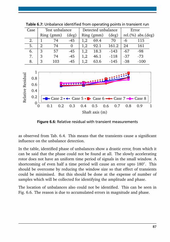
Table 6.7: Unbalance identified from operating points in transient runCase Test unbalance Detected unbalance Error

Ring (gmm) (deg) Ring (gmm) (deg) rel.(%) abs.(deg)2. 1 74 -45 1,2 69.4 70 -6 1155. 2 74 0 1,2 92.1 161.2 24 1616. 3 57 -45 1,2 18.3 -143 -67 -987. 3 74 -45 1,2 46.1 -118 -37 -738. 3 103 -45 1,2 63.6 -145 -38 -100

0 0.1 0.2 0.3 0.4 0.5 0.6 0.7 0.8 0.9 10

0.2

0.40.6

0.8

1

Shaft axis (m)

Rel

ativ

eR

esid

ual

Case 2 Case 5 Case 6 Case 7 Case 8

Figure 6.6: Relative residual with transient measurements

as observed from Tab. 6.4. This means that the transients cause a significantinfluence on the unbalance detection.

In the table, identified phase of unbalances show a drastic error, from which itcan be said that the phase could not be found at all. The slowly acceleratingrotor does not have an uniform time period of signals in the small window. Ashortcoming of even half a time period will cause an error upto 180. Thisshould be overcome by reducing the window size so that effect of transientscould be minimised. But this should be done at the expense of number ofsamples which will be collected for identifying the amplitude and phase.

The location of unbalances also could not be identified. This can be seen inFig. 6.6. The reason is due to accumulated errors in magnitude and phase.

87

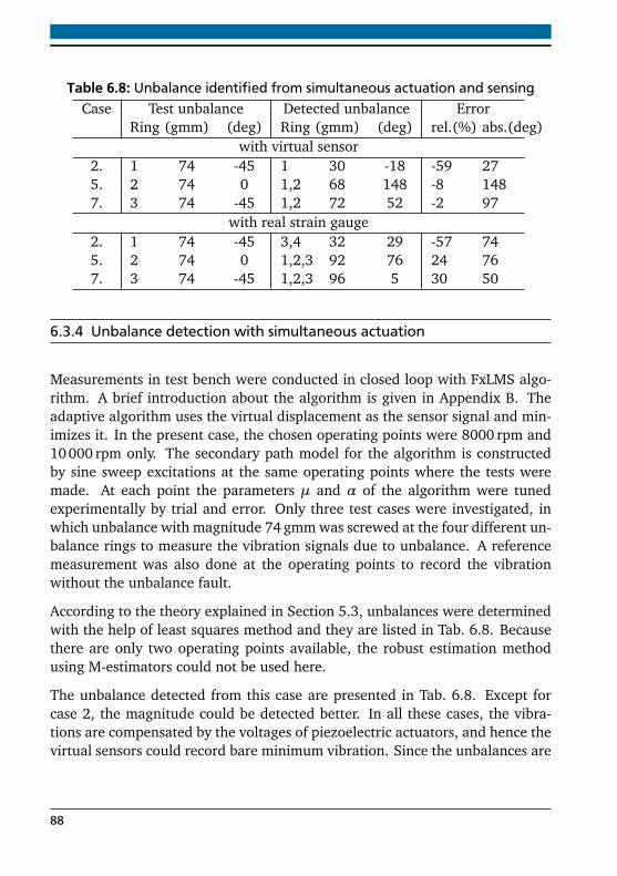
Table 6.8: Unbalance identified from simultaneous actuation and sensingCase Test unbalance Detected unbalance Error

Ring (gmm) (deg) Ring (gmm) (deg) rel.(%) abs.(deg)with virtual sensor

2. 1 74 -45 1 30 -18 -59 275. 2 74 0 1,2 68 148 -8 1487. 3 74 -45 1,2 72 52 -2 97

with real strain gauge2. 1 74 -45 3,4 32 29 -57 745. 2 74 0 1,2,3 92 76 24 767. 3 74 -45 1,2,3 96 5 30 50

6.3.4 Unbalance detection with simultaneous actuation

Measurements in test bench were conducted in closed loop with FxLMS algo-rithm. A brief introduction about the algorithm is given in Appendix B. Theadaptive algorithm uses the virtual displacement as the sensor signal and min-imizes it. In the present case, the chosen operating points were 8000 rpm and10000 rpm only. The secondary path model for the algorithm is constructedby sine sweep excitations at the same operating points where the tests weremade. At each point the parameters µ and α of the algorithm were tunedexperimentally by trial and error. Only three test cases were investigated, inwhich unbalance with magnitude 74 gmm was screwed at the four different un-balance rings to measure the vibration signals due to unbalance. A referencemeasurement was also done at the operating points to record the vibrationwithout the unbalance fault.

According to the theory explained in Section 5.3, unbalances were determinedwith the help of least squares method and they are listed in Tab. 6.8. Becausethere are only two operating points available, the robust estimation methodusing M-estimators could not be used here.

The unbalance detected from this case are presented in Tab. 6.8. Except forcase 2, the magnitude could be detected better. In all these cases, the vibra-tions are compensated by the voltages of piezoelectric actuators, and hence thevirtual sensors could record bare minimum vibration. Since the unbalances are

88

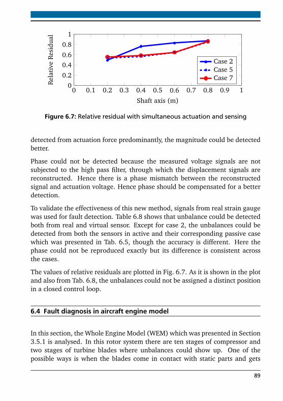
0 0.1 0.2 0.3 0.4 0.5 0.6 0.7 0.8 0.9 10

0.2

0.40.6

0.8

1

Shaft axis (m)

Rel

ativ

eR

esid

ual

Case 2Case 5Case 7

Figure 6.7: Relative residual with simultaneous actuation and sensing

detected from actuation force predominantly, the magnitude could be detectedbetter.

Phase could not be detected because the measured voltage signals are notsubjected to the high pass filter, through which the displacement signals arereconstructed. Hence there is a phase mismatch between the reconstructedsignal and actuation voltage. Hence phase should be compensated for a betterdetection.

To validate the effectiveness of this new method, signals from real strain gaugewas used for fault detection. Table 6.8 shows that unbalance could be detectedboth from real and virtual sensor. Except for case 2, the unbalances could bedetected from both the sensors in active and their corresponding passive casewhich was presented in Tab. 6.5, though the accuracy is different. Here thephase could not be reproduced exactly but its difference is consistent acrossthe cases.

The values of relative residuals are plotted in Fig. 6.7. As it is shown in the plotand also from Tab. 6.8, the unbalances could not be assigned a distinct positionin a closed control loop.

6.4 Fault diagnosis in aircraft engine model

In this section, the Whole Engine Model (WEM) which was presented in Section3.5.1 is analysed. In this rotor system there are ten stages of compressor andtwo stages of turbine blades where unbalances could show up. One of thepossible ways is when the blades come in contact with static parts and gets

89

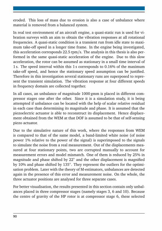
eroded. This loss of mass due to erosion is also a case of unbalance wherematerial is removed from a balanced system.

In real test environment of an aircraft engine, a quasi-static run is used for vi-bration surveys with an aim to obtain the vibration responses at all rotationalfrequencies. A quasi-static condition is a transient run from idle state to maxi-mum take-off speed in a longer time frame. In the engine being investigated,this acceleration corresponds 22.5 rpm/s. The analysis in this thesis is also per-formed in the same quasi-static acceleration of the engine. Due to this slowacceleration, the rotor can be assumed as stationary in a small time interval of1 s. The speed interval within this 1 s corresponds to 0.16% of the maximumtake-off speed, and hence the stationary speed assumption can be justified.Therefore in this investigation several stationary runs are superposed to repre-sent the transient simulation. The vibration response at four different speedsin frequency domain are collected together.

In all cases, an unbalance of magnitude 1000 gmm is placed in different com-pressor stages one after the other. Since it is a simulation study, it is beingattempted if unbalance can be located with the help of scalar relative residualin each case than determining its magnitude and phase. It is assumed that thepiezoelectric actuator is able to reconstruct its displacement. Hence displace-ment obtained from the WEM at that DOF is assumed to be that of self-sensingpiezo actuator.

Due to the simulative nature of this work, where the responses from WEMis compared to that of the same model, a band-limited white noise (of noisepower 1% relative to the power of the signal) is superimposed to the signalsto simulate the noise from a real measurement. Out of the displacements mea-sured at four stationary points, two are corrupted manually to account formeasurement errors and model mismatch. One of them is reduced by 25% inmagnitude and phase shifted by 22 and the other displacement is magnifiedby 10% and phase shifted by 135. They represent the outliers for the optimi-sation problem. Later with the theory of M-estimators, unbalances are detectedagain in the presence of this error and measurement noise. On the whole, thethree actuator positions are analysed for three separate cases.

For better visualisation, the results presented in this section contain only unbal-ances placed in three compressor stages (namely stages 3, 6 and 10). Becausethe centre of gravity of the HP rotor is at compressor stage 6, these selected

90

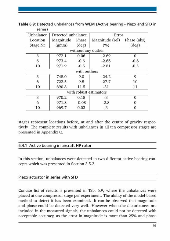
Table 6.9: Detected unbalances from WEM (Active bearing - Piezo and SFD inseries)

Unbalance Detected unbalance ErrorLocation Magnitude Phase Magnitude (rel) Phase (abs)Stage Nr. (gmm) (deg) (%) (deg)

without any outlier3 972.1 0.06 -2.69 06 973.4 -0.6 -2.66 -0.6

10 971.9 -0.5 -2.81 -0.5with outliers

3 748.0 9.0 -24.2 96 722.5 9.8 -27.7 10

10 690.8 11.5 -31 11with robust estimators

3 970.2 0.18 -3 06 971.8 -0.08 -2.8 0

10 969.7 0.03 -3 0

stages represent locations before, at and after the centre of gravity respec-tively. The complete results with unbalances in all ten compressor stages arepresented in Appendix C.

6.4.1 Active bearing in aircraft HP rotor

In this section, unbalances were detected in two different active bearing con-cepts which was presented in Section 3.5.2.

Piezo actuator in series with SFD

Concise list of results is presented in Tab. 6.9, where the unbalances wereplaced at one compressor stage per experiment. The ability of the model-basedmethod to detect it has been examined. It can be observed that magnitudeand phase could be detected very well. However when the disturbances areincluded in the measured signals, the unbalances could not be detected withacceptable accuracy, as the error in magnitude is more than 25% and phase

91

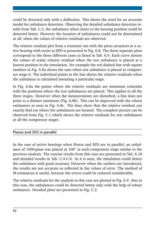
could be detected only with a deflection. This shows the need for an accuratemodel for unbalance detection. Observing the detailed unbalance detection re-sults from Tab. C.2, the unbalance when closer to the bearing position could bedetected better. However the location of unbalances could not be determinedat all, when the values of relative residuals are observed.

The relative residual plot from a transient run with the piezo actuators in a ac-tive bearing with series in SFD is presented in Fig. 6.8. The three separate plotscorrespond to the three different cases as listed in Tab. 6.9. Each curve denotethe values of scalar relative residual when the test unbalance is placed at aknown position in the simulation. For example the red dashed line with squaremarkers in Fig. 6.8a shows the case when test unbalance is placed at compres-sor stage 6. The individual points in the line shows the relative residuals whenthe unbalance is calculated assuming a particular stage.

In Fig. 6.8a the points where the relative residuals are minimum coincideswith the positions where the test unbalances are placed. This applies to all thethree stages. However when the measurements are disturbed, a line does notpoint to a distinct minimum (Fig. 6.8b). This can be improved with the robustestimators as seen in Fig. 6.8c. The lines show that the relative residual canexactly find out where the unbalances are located. The complete picture can beobserved from Fig. C.1 which shows the relative residuals for test unbalancesat all the compressor stages.

Piezos and SFD in parallel

In the case of active bearings when Piezos and SFD are in parallel, an unbal-ance of 1000 gmm was placed at 100 at each compressor stage similar to theprevious analysis. The concise results from this case are presented in Tab. 6.10and detailed results in Tab. C.4-C.6. As it is seen, the simulation could detectthe unbalance with good accuracy. However when the outliers are introduced,the results are not accurate as reflected in the values of error. The method ofM-estimators is useful, because the errors could be reduced considerably.

The relative residuals for the analysis in this case are plotted in Fig. 6.9. Also inthis case, the unbalances could be detected better only with the help of robustestimators. Detailed plots are presented in Fig. C.2.

92

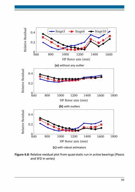
600 800 1000 1200 1400 16000

0.2

0.4

HP Rotor axis (mm)

Rel

ativ

eR

esid

ual

Stage3 Stage6 Stage10

(a) without any outlier

600 800 1000 1200 1400 1600 18000

0.2

0.4

HP Rotor axis (mm)

Rel

ativ

eR

esid

ual

(b) with outliers

600 800 1000 1200 1400 1600 18000

0.2

0.4

HP Rotor axis (mm)

Rel

ativ

eR

esid

ual

(c) with robust estimators

Figure 6.8: Relative residual plot from quasi-static run in active bearings (Piezosand SFD in series)

93

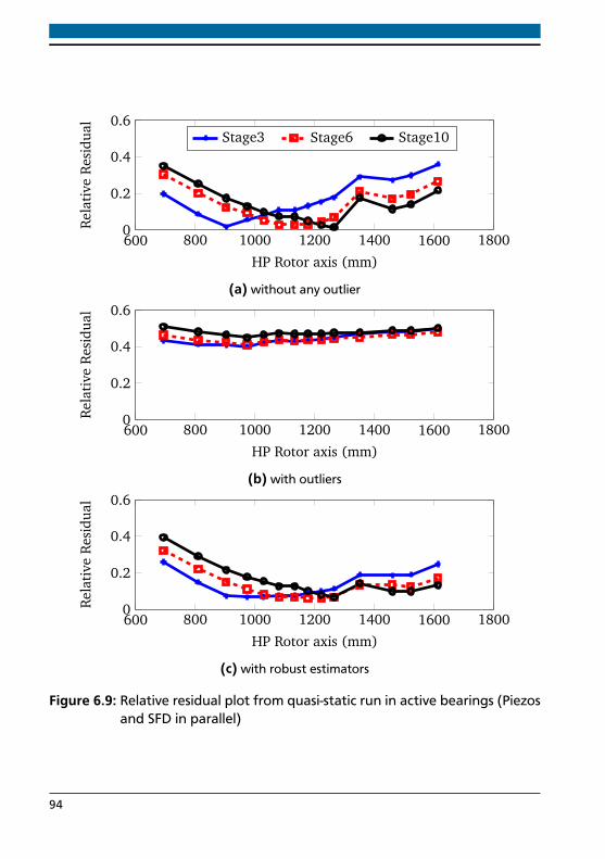
600 800 1000 1200 1400 1600 18000

0.2

0.4

0.6

HP Rotor axis (mm)

Rel

ativ

eR

esid

ual

Stage3 Stage6 Stage10

(a) without any outlier

600 800 1000 1200 1400 1600 18000

0.2

0.4

0.6

HP Rotor axis (mm)

Rel

ativ

eR

esid

ual

(b) with outliers

600 800 1000 1200 1400 1600 18000

0.2

0.4

0.6

HP Rotor axis (mm)

Rel

ativ

eR

esid

ual

(c) with robust estimators

Figure 6.9: Relative residual plot from quasi-static run in active bearings (Piezosand SFD in parallel)

94

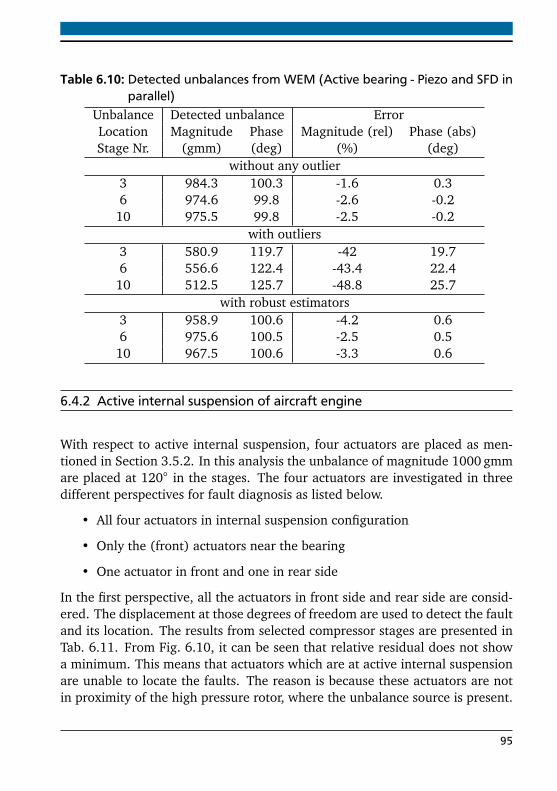
Table 6.10: Detected unbalances from WEM (Active bearing - Piezo and SFD inparallel)

Unbalance Detected unbalance ErrorLocation Magnitude Phase Magnitude (rel) Phase (abs)Stage Nr. (gmm) (deg) (%) (deg)

without any outlier3 984.3 100.3 -1.6 0.36 974.6 99.8 -2.6 -0.2

10 975.5 99.8 -2.5 -0.2with outliers

3 580.9 119.7 -42 19.76 556.6 122.4 -43.4 22.4

10 512.5 125.7 -48.8 25.7with robust estimators

3 958.9 100.6 -4.2 0.66 975.6 100.5 -2.5 0.5

10 967.5 100.6 -3.3 0.6

6.4.2 Active internal suspension of aircraft engine

With respect to active internal suspension, four actuators are placed as men-tioned in Section 3.5.2. In this analysis the unbalance of magnitude 1000 gmmare placed at 120 in the stages. The four actuators are investigated in threedifferent perspectives for fault diagnosis as listed below.

• All four actuators in internal suspension configuration

• Only the (front) actuators near the bearing

• One actuator in front and one in rear side

In the first perspective, all the actuators in front side and rear side are consid-ered. The displacement at those degrees of freedom are used to detect the faultand its location. The results from selected compressor stages are presented inTab. 6.11. From Fig. 6.10, it can be seen that relative residual does not showa minimum. This means that actuators which are at active internal suspensionare unable to locate the faults. The reason is because these actuators are notin proximity of the high pressure rotor, where the unbalance source is present.

95

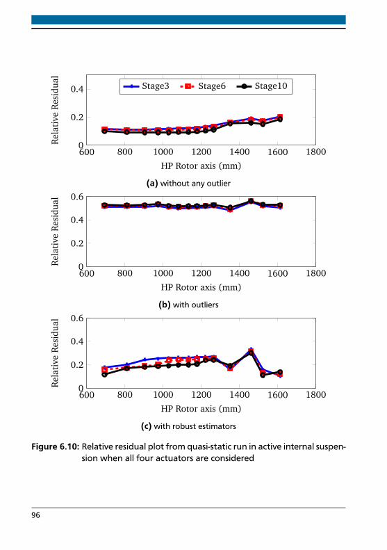
600 800 1000 1200 1400 1600 18000

0.2

0.4

HP Rotor axis (mm)

Rel

ativ

eR

esid

ual

Stage3 Stage6 Stage10

(a) without any outlier

600 800 1000 1200 1400 1600 18000

0.2

0.4

0.6

HP Rotor axis (mm)

Rel

ativ

eR

esid

ual

(b) with outliers

600 800 1000 1200 1400 1600 18000

0.2

0.4

0.6

HP Rotor axis (mm)

Rel

ativ

eR

esid

ual

(c) with robust estimators

Figure 6.10: Relative residual plot from quasi-static run in active internal suspen-sion when all four actuators are considered

96

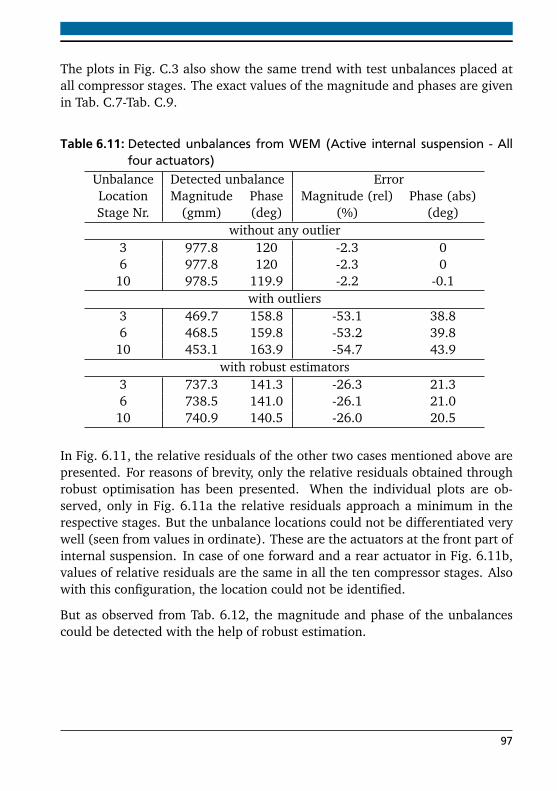
The plots in Fig. C.3 also show the same trend with test unbalances placed atall compressor stages. The exact values of the magnitude and phases are givenin Tab. C.7-Tab. C.9.

Table 6.11: Detected unbalances from WEM (Active internal suspension - Allfour actuators)

Unbalance Detected unbalance ErrorLocation Magnitude Phase Magnitude (rel) Phase (abs)Stage Nr. (gmm) (deg) (%) (deg)

without any outlier3 977.8 120 -2.3 06 977.8 120 -2.3 0

10 978.5 119.9 -2.2 -0.1with outliers

3 469.7 158.8 -53.1 38.86 468.5 159.8 -53.2 39.8

10 453.1 163.9 -54.7 43.9with robust estimators

3 737.3 141.3 -26.3 21.36 738.5 141.0 -26.1 21.0

10 740.9 140.5 -26.0 20.5

In Fig. 6.11, the relative residuals of the other two cases mentioned above arepresented. For reasons of brevity, only the relative residuals obtained throughrobust optimisation has been presented. When the individual plots are ob-served, only in Fig. 6.11a the relative residuals approach a minimum in therespective stages. But the unbalance locations could not be differentiated verywell (seen from values in ordinate). These are the actuators at the front part ofinternal suspension. In case of one forward and a rear actuator in Fig. 6.11b,values of relative residuals are the same in all the ten compressor stages. Alsowith this configuration, the location could not be identified.

But as observed from Tab. 6.12, the magnitude and phase of the unbalancescould be detected with the help of robust estimation.

97

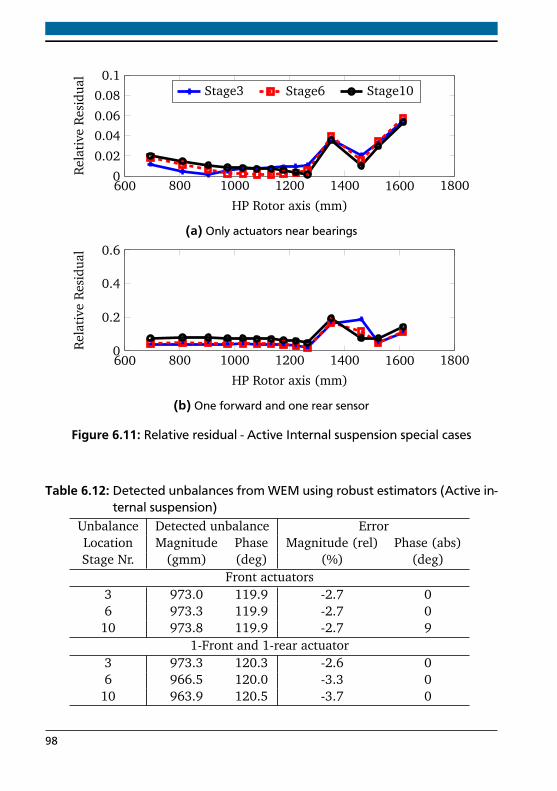
600 800 1000 1200 1400 1600 18000

0.02

0.040.06

0.08

0.1

HP Rotor axis (mm)

Rel

ativ

eR

esid

ual

Stage3 Stage6 Stage10

(a) Only actuators near bearings

600 800 1000 1200 1400 1600 18000

0.2

0.4

0.6

HP Rotor axis (mm)

Rel

ativ

eR

esid

ual

(b) One forward and one rear sensor

Figure 6.11: Relative residual - Active Internal suspension special cases

Table 6.12: Detected unbalances from WEM using robust estimators (Active in-ternal suspension)

Unbalance Detected unbalance ErrorLocation Magnitude Phase Magnitude (rel) Phase (abs)Stage Nr. (gmm) (deg) (%) (deg)

Front actuators3 973.0 119.9 -2.7 06 973.3 119.9 -2.7 010 973.8 119.9 -2.7 9

1-Front and 1-rear actuator3 973.3 120.3 -2.6 06 966.5 120.0 -3.3 010 963.9 120.5 -3.7 0

98

6.5 Discussion

Important observations from fault detection in both the rotor systems are pre-sented in this section.

6.5.1 Observations from fault diagnosis in test bench

The time domain fault diagnosis method is computationally expensive method.The information of the model is used multiple times within the same executionwhich magnifies the error in the model. Hence the frequency domain methodusing parameter estimation techniques was preferred in this thesis.

The bearing displacements are used for fault detection. The least squaresmethod could detect unbalance faults with respect to their magnitude, phaseand location very good. However when real measured data was analysed,the WLS method is used which is more robust against outliers in the data.Three different experiments were carried out. The first is at stationary op-erating points between the first two resonances. The second is a transientmeasurement at a specified acceleration. The third experiment in closed loopmeasurement with simultaneous actuation and sensing.

In the stationary experiments, 11 cases of test unbalances were examined. Itwas observed that a relative deviation of at least one unit is necessary be-tween the balanced and unbalanced signals for a detection to be possible. Thiscondition was matched by all the test cases except for two. These two casescorrespond to low test masses at rings farther from the active bearing. Unbal-ances in ring 4 could not be detected due to the presence of an anti-resonanceat the operating range of this experiment. Because the unbalance from theestimation method is determined as a complex number, the same condition ap-plies to detect the phase also. The detected unbalances from other sensors alsoyielded comparable results, thus proving the ability of piezoelectric actuator tobe used as a sensor.

For transient analysis five test cases were selected. The detected magnitudesare lesser than those detected in stationary experiments, though the relativeerrors are acceptable. This is due to the effect of transients affecting the sig-nals. Detecting phase is difficult in this case as the transient sinus signals from

99

sensors are only approximately useful in determining the phase. The accumu-lated error in detecting magnitude and phase reflects on location identificationalso, which makes it ambiguous.

Another important contribution of this thesis is the unbalance detection withan adaptive control algorithm in closed loop. This method which is extendedfrom the existing parameter estimation method uses both the actuation voltageand reconstructed signals for fault detection. Though magnitude of unbalancescould be determined, the phases need to be compensated for a mismatch dueto filtering. This extended method was also validated with real strain gauges.The unbalances could also be detected from them similar to the virtual sensors.Hence the virtual sensors are capable of detecting unbalances in passive caseand in a closed control loop.

6.5.2 Observations from fault diagnosis in WEM

In the HP rotor of the WEM, unbalances arising from one of its compressorstages is diagnosed. Mainly two actuator placement positions are analysed.The actuators at the bearings of the HP rotor is the first position. Out oftwo different configurations theoretically investigated, both are able to diag-nose unbalance faults. The diagnosis method needs a robust estimator such asWLS analysed in this thesis. Only due to them a better detection of unbalancemagnitude and phase could be possible.

The second actuator position which was examined is the active internal sus-pension. Because the actuators are not near the source of vibrations, thisconstellation of actuators could not locate the unbalances. The four actua-tors employed in this configuration could not locate the unbalance precisely.Two special cases were formulated and analysed separately. The first caseconsidered only two actuators near the HP rotor bearing. The second caseconsidered one actuator in the front and one at the rear. Though the formercase could locate the unbalance, it is very insignificant.

An interesting phenomenon could be observed in the active internal suspensionconfiguration. Though there is more information available when signals fromfour actuators are measured, results from them are not better than with lessactuators. This could be observed from Tab. 6.11 and Tab. 6.12. The reason isdue to positioning of the actuators in the rear links (Fig. 3.20b). The vibrationis transmitted radially from the HP rotor towards the casing. But the rear links

100

are not arranged radially when compared with the front links (Fig. 3.20a). Alsothe plane of the rear links is away from the HP rotor. Due to these reasons, theactuators mounted in rear links worsen the estimation of unbalance.

Hence it can be concluded that only actuators if placed in the active bear-ing could diagnose unbalances. From a fault diagnosis perspective both theconcepts namely actuators in parallel or in series with SFD could be imple-mented.

6.5.3 Final remarks

There is however a difference between the experiments carried out in WEM andthe scaled rotor test bench. In WEM the unbalances were added at differentcompressor stages. Each individual compressor stage is comparable to eachother in terms of mass and stiffness. They are also more or less symmetricallydistributed along the length of the HP rotor.

But in the scaled rotor test bench this is not the case. The individual balancingrings are situated in the same rotor shaft with a turbine dummy. The mass andstiffness of the rotating disc are higher than those of the rings. Hence only testunbalances in balancing rings away from the disc could be detected. This isalso evident from the values of relative residuals which indicate the presenceof faults in the first two rings only. When the method would be transferred tothe real aircraft engine, this problem would already get addressed.

On the other hand, measurements in real test bench were performed consider-ing the temperature of the actuator as well. The experiments were only donewhen the temperature of the actuator was less than 35 C. The intention be-hind it is to avoid any temperature dependent non-linearities affecting the faultdetection. However this is very significant in real aircraft engine. Though itslocation would be away from the hot gases from the combustion chamber, themodel should be extended to include these effects.

101

7 Conclusion and OutlookThe main objective of this thesis is to use self-sensing piezoelectric actuatorsfor a model based fault diagnosis problem in rotor systems. In order to achievethis, the problem has been broken down into modules. The individual modulesare presented in this chapter and the complete picture described. In the end,indicators towards future works are presented.

7.1 Summary of the thesis

Two rotor systems were investigated in this thesis, one is an aircraft engine andother a simple rotor test bench. A finite element model of the former was de-veloped by its manufacturer in which piezoelectric actuators were included asspring elements. The FE model of test bench has been improved from previousworks with the help of grey-box modelling techniques. Frequency responsefunction from real test bench was obtained by chirp excitations from piezo-electric actuators. The tuned model was validated with measurements fromimpulse hammer excitation, as they better represent the transmission of forcesat the unbalance rings to all the sensors available in the test bench.

There are four piezoelectric actuators in the test bench, to actively controlvibration arising out of unbalance excitation. Self-sensing techniques wereapplied to reconstruct the displacement in two of the actuators. Here the elec-trical signals of the actuators such as voltage and current are used to derive themechanical displacement. The reconstruction is achieved in a two step process.For capacitance identification, anti-resonance frequencies were identified fromthe frequency response function. The ability of the actuator to act as a sensorwas proven in both at a stationary operating point in time-domain and acrossthe operating frequency range in frequency domain. The reconstructed dis-placement signals are used in closed loop with a PPF controller. This controllercould reduce the resonance peak by approximately 33%. The actuation volt-age needed was only 30-40 V, which is well within the linear range of actuatoroperation. At a point away from the resonance, the reconstructed signals were

103

used in closed loop with an adaptive algorithm. This proves the effectivenessof actuators in simultaneous actuation and sensing.

Faults in the rotor system were diagnosed in frequency domain using parame-ter estimation techniques. As a precursor towards future works, only unbalancefault was investigated. Least squares approach was used to detect the magni-tude and faults of unbalance, which inturn uses an L2 norm to find an optimalvalue. Robustness of LS approach was improved by Weighted least squares(WLS), with weights derived from method of M-estimators. To identify the lo-cation of faults, a scalar relative residual was calculated. The algorithm hasbeen extended to be used in a closed control loop by including the actuationforce due to actuator voltage.

Initially simulations were performed with the model of rotor test bench. Theproblem of outliers in signals were effectively handled with WLS. Unbalancemagnitude, phase and location could be identified with the help of weightedleast squares better. The same was identified with the help of measured signalsfrom test bench. The identified results from reconstructed displacement sig-nals due to self-sensing are compared against those measured from real straingauges and a good agreement can be seen. Apart from stationary speeds, theability to diagnose faults in a transient condition was shown. As a final and im-portant step, fault was detected under simultaneous actuation and sensing ina closed loop. In these last two experiments, only unbalance magnitude couldbe determined.

Fault diagnosis was also carried out using model of high pressure rotor of anaircraft engine. It has been assumed that mechanical displacement could beextracted from piezos mounted at three different locations. In simulations,outliers were introduced into the data and performance evaluated. Unbalancemagnitude, phase and location could be detected only in those locations whenthe actuators are placed in the bearings, because they are closer to the rotor.

7.2 Inference

It can be concluded from this thesis that bearing displacement signals could beused in estimation of faults. These displacement signals could be reconstructedfrom electrical signals of the piezoelectric actuator at the bearings. For thedetection to be possible, a relative deviation of sensor signals of value one unitis a threshold. Mass in the test bench is asymmetrically distributed due to the

104

rotating disc at a farther end. Because of this unbalances only away from itcould be detected. However in a real HP rotor of an aircraft engine, the massis symmetrically distributed in its shaft and faults could be detected in all thestages.

The virtual sensors due to reconstruction in piezoelectric actuators indicate agood potential to replace the real sensors. Though not in its present form,unbalances could be detected also from virtual sensors in a closed loop withsimultaneous actuation of piezoelectric actuators.

7.3 Future works

In a nutshell it can be said that this research work has taken on the unbal-ance detection problem using conventional detection methods using a newlydeveloped virtual sensor. In future, there could be works to investigate the rel-evance of this sensor in detecting other faults. Apart from rotation synchronousvibrations, faults such as misalignment, gear defects create super-synchronousvibrations. However their analysis with available test bench needs some con-structional modification. Considering the weight of the rotating components,shaft cracks could make experimental investigations dangerous. Neverthelessbearing faults are relatively easier to be realised.

Before the multiples of synchronous speed vibrations could be analysed, thereis a need to develop virtual sensor. With reference to Fig.4.10, the high passfilter restricts the operating range between 50-230 Hz. A third possible exten-sion is to include temperature dependent effects of the actuator into the systemmodel.

105

Bibliography[1] J. Vance, F. Zeidan, and B. Murphy, Machinery Vibration and Rotordynam-

ics. John Wiley & Sons Inc., 2010.

[2] A. Preumont, Vibration Control of Active Structures- An Introduction,3rd ed. Springer, 2011.

[3] Mechanical vibration - Rotor balancing - Part 14: Procedures for assess-ing balance errors, International Standards Organisation Std. ISO 21 940-14:2012.

[4] F. Lebo, “Theoretische und experimentelle Analysen von Flugtriebwerk-srotoren zur aktiven Schwingungsminderung mit Piezostapelaktoren,”Ph.D. dissertation, Technische Universität Darmstadt, 2011.

[5] S. Ding, Model-based Fault diagnosis techniques- Design schemes, Algo-rithms and tools. Springer, 2008.

[6] R. Isermann, “Model-based fault-detection and diagnosis - status and ap-plications,” Annual Reviews in Control, vol. 29, pp. 71–85, 2005.

[7] Z. Wang, R. S. Schittenhelm, and S. Rinderknecht, “Observer design forunbalance excited rotor systems with gyroscopic effect,” in Proceedingsof 2012 IEEE International Conference on Mechatronics and Automation,August 5-8 2012, pp. 7–12.

[8] R. Ambur, Z. Wang, R. S. Schittenhelm, and S. Rinderknecht, “Model-based fault detection on a non-linear rotor system,” in Proceedings of the9th IFToMM International Conference on Rotor Dynamics, 2015.

[9] M. Witczak, Modelling and Estimation strategies for Fault Diagnosis ofNon-Linear Systems. From Analytical to Soft Computing Approaches. Lec-ture Notes in Control and Information Sciences. Springer Verlag, 2007.

[10] R. Walker, S. Perinpanayagam, and I. K. Jennions, “Rotordynamic faults:Recent advances in diagnosis and prognosis,” International Journal of Ro-tating Machinery, vol. 2013, pp. 1–12, 2013.

[11] J. M. Corres, J. Bravo, and F. J. Arregui, “Unbalance and harmonics de-tection in induction motors using an optical fiber sensor,” IEEE SensorsJournal, vol. 6, no. 3, pp. 605–612, 2006.

107

[12] Q. Han, Z. Zhang, and B. Wen, “Periodic motions of a dual-disc rotorsystem with rub-impact at fixed limiter,” Proceedings of the Institution ofMechanical Engineers, Part C: Journal of Mechanical Engineering Science,vol. 222, no. 10, pp. 1935–1946, 2008.

[13] S. Ganeriwala, B. Schwarz, and M. H. Richardson, “Operating deflectionshapes detect unbalance in rotating equipment,” Journal of Sound andVibration, vol. 43, no. 5, pp. 11–13, 2009.

[14] R. Ambur, R. S. Vadamalu, and S. Rinderknecht, “Identification of unbal-ance faults in rotors with unknown input observers using classical andLMI based approaches,” in European Control Conference 2016, 2016.

[15] H. Wang, J. Wang, and J. Lam, “Robust fault detection observer design:Iterative LMI approaches,” Journal of Dynamic Systems, Measurement andControl, vol. 129, no. 1, pp. 77–82, 2007.

[16] Z. Wang, A. Wahrburg, and S. Rinderknecht, “Consideration of gyroscopiceffect in fault detection and isolation for unbalance excited rotor sys-tems,” International Journal of Rotating Machinery, vol. 2012, pp. 1–14,2012.

[17] C. Zang, A. W. Lees, and M. I. Friswell, Multi plane balancing of a rotatingmachine using a single transducer, 2002, pp. 130 – 136.

[18] R. Markert, R. Platz, and M. Seidler, “Model based fault identification inrotor systems by least squares fitting,” International Journal of RotatingMachinery, vol. 7, no. 5, pp. 311–321, 2001.

[19] R. Platz, “Untersuchungen zur modellgestützten Diagnose von Un-wuchten und Wellenrissen in Rotorsystemen,” Ph.D. dissertation, Tech-nische Universität Darmstadt, Düsseldorf, 2004.

[20] G. N. D. S. Sudhakar and A. S. Sekhar, “Identification of unbalance in arotor bearing system,” Journal of Sound and Vibration, vol. 330, no. 10,pp. 2299–2313, 2011.

[21] N. Bachschmid, P. Pennacchi, and A. Vania, “Identification of multiplefaults in rotor systems,” Journal of Sound and Vibration, vol. 254, no. 2,pp. 327 – 366, 2002.

108

[22] N. Bachschmid, P. Pennacchi, A. Vania, G. Zanetta, and L. Gregori, “Casestudies of fault identification in power plant large rotating machinery,” inProceedings of the IFToMM-6th International Conference on Rotor Dynam-ics, 2002, pp. 191–200.

[23] A. Lees, J. K. Sinha, and M. I. Friswell, “Model-based identification ofrotating machines,” Mechanical Systems and Signal Processing, vol. 23,no. 6, pp. 1884 – 1893, 2009.

[24] S. Hawibowo, “Sicherheitstechnische abschätzung des betriebszustandesvon pumpen zur schadensfrüherkennung,” Ph.D. dissertation, TechnischeUniversität Berlin, 1997.

[25] M. Atalla and D. Inman, “On model updating using neural networks,”Mechanical Systems and Signal Processing, vol. 12, no. 1, pp. 135 – 161,1998.

[26] J. Mottershead and M. Friswell, “Model updating in structural dynamics:A survey,” Journal of Sound and Vibration, vol. 167, no. 2, pp. 347 – 375,1993.

[27] A. Younan and A. El-Shafei, “Model calibration of anisotropic rotordy-namic systems with speed-dependent parameters,” Journal of Engineeringfor Gas Turbines and Power, vol. 130, 2008.

[28] T. Marwala, Finite-element-model Updating Using Computational Intelli-gence Techniques, Applications to Structural Dynamics. Springer London,2010.

[29] D. Ewins, Modal Testing: Theory and Practice. Brüel & Kjær, 1986.

[30] H. Irretier, “Mathematical foundations of experimental modal analysis inrotor dynamics,” Mechanical Systems and Signal Processing, vol. 13, no. 2,pp. 183 – 191, 1999.

[31] M. Aenis, “Einsatz aktiver Magnetlager zur modellbasierten Fehlerdiag-nose in einer Kreiselpumpe,” Ph.D. dissertation, Technische UniversitätDarmstadt, Darmstadt, 2002.

[32] N. Butzek, “Modellbasierte Verfahren zur online Fehlerdiagnose an einerKreiselpumpe in aktiven Magnetlagern,” Ph.D. dissertation, TechnischeUniversität Darmstadt, 2009.

109

[33] B. Hasch, “Modellbasierte Fehlererkennung an einem elastischen Rotormit Hilfe aktiver Lagerung,” Ph.D. dissertation, Technische UniversitätDarmstadt, 2010.

[34] Z. Wang, “Robuste modellbasierte Fehlerdiagnose an elastischen Rotorenunter Berücksichtigung der Gyroskopie,” Ph.D. dissertation, TechnischeUniversität Darmstadt, 2013.

[35] K. Mühlenfeld, A. Rienäcker, C. Streller, and L. Padva, “Vibration reduc-tion in aero-engine- a case study,” in Schwingungen in Rotierenden Maschi-nen, 2001, pp. 261–268.

[36] J. M. Barragán, “Engine vibration monitoring and diagnosis based onon-board captured data,” in RTO AVT Symposium on "Ageing Mechanismsand Control: Part B- Monitoring and Management of Gas Turbine Fleets forExtended Life and Reduced Costs", 2001.

[37] B. Domes, “Vibration phenomena in aero-engines,” in 9th InternationConference on Vibrations in Rotating Machinery IMechE, 2008.

[38] G. P. Whiteford and P. T. Herbst, “Vibration isolation system including apassive tuned vibration absorber,” USA Patent US5 687 948, November18, 1997.

[39] A. El-Shafei, “Unbalance response of a jeffcott rotor incorporating longsqueeze film dampers,” ASME Journal of Vibration and Acoustics, vol. 113,pp. 85–94, 1991.

[40] A. El-Shafei, “Experimental and analytical investigation of hybrid squeezefilm dampers,” ASME Journal of Eng Gas Turbines Power, vol. 115, no. 2,pp. 353–359, 1993.

[41] D. Hodgson and T. Duclos, “Mount with adjustable length inertia track,”USA Patent 4 969 632, November 13, 2000.

[42] M. H. Taha, “Power electronics application for more electric aircraft,”Recent Advances in Aircraft Technology, vol. 14, pp. 289–308, 2012.

[43] A. Palazzolo, R. Lin, R. Alexander, A. Kascak, and J. Montague, “Piezo-electric pushers for active vibration control of rotating machinery,” ASMEJournal of Vibration and Acoustics, Stress and Reliability, vol. 111, no. 3,pp. 298–305, 1989.

110

[44] A. Palazzolo, R. Lin, R. Alexander, A. Kascak, and J. Montague, “Testand theory for piezoelectric actuator- active vibration control of rotatingmachinery,” ASME Journal of Vibration and Acoustics, vol. 113, no. 2, pp.167–175, 1991.

[45] M. Borsdorf, “Aktive Schwingungsminderung elastischer Flugtriebwerk-srotoren mit Piezostapelaktoren unter Berücksichtigung der Dynamik desTriebwerkgehäuses,” Ph.D. dissertation, Technische Universität Darm-stadt, 2014.

[46] R. S. Schittenhelm, “Regelungstechnische Verfahren zur aktiven Min-derung von Rotorschwingungen,” Ph.D. dissertation, Technische Univer-sität Darmstadt, 2015.

[47] F. Becker, “Active vibration isolation of a flexible rotor being subject tounbalance excitation and gyroscopic effect using H∞ optimal control.” inProceedings of the 9th IFToMM International Conference on Rotor Dynam-ics, 2015.

[48] F. Becker, M. A. Sehr, and S. Rinderknecht, “Gain-scheduled h∞-controlfor active vibration isolation of a gyroscopic rotor.” in ASME 2015 Con-ference on Smart Materials, Adaptive Structures and Intelligent Systems,2015.

[49] S. Heindel, F. B. Becker, and S. Rinderknecht, “Unbalance and resonanceelimination with active bearings on a jeffcott rotor,” Mechanical Systemsand Signal Processing, vol. 85, pp. 339–353, 2016.

[50] E. Anderson and N. Hagood, “Simultaneous piezoelectric sens-ing/actuation: Analysis and application to controlled structures,” Journalof Sound and Vibration, vol. 174, no. 5, pp. 617 – 639, 1994.

[51] D. G. Cole and R. L. Clark, “Adaptive compensation of piezoelectric senso-riactuators,” Journal of Intelligent Material Systems and Structures, vol. 5,pp. 665–672, 1994.

[52] E. Grasso, N. Totaro, H. Janocha, and D. Naso, “Piezoelectric self sensingactuators for high voltage excitation,” Smart Materials and Structures,vol. 22, no. 6, 2013.

[53] R. Köhler, “Phänomenologische Modellierung des temperaturabhängigenVerhaltens piezoelektrischer Stapelaktoren,” Ph.D. dissertation, Technis-che Universität Darmstadt, 2013.

111

[54] H. Janocha, Unkonventionelle Aktoren- Eine Einführung. OldenbourgVerlag, 2010.

[55] E. Grasso, “Self sensing techniques for piezoelectric vibration applica-tions,” Ph.D. dissertation, Universität Saarlandes, Saarbrücken, 2013.

[56] R. Deibert, “Methoden zur Fehlererkennung an Komponenten imgeschlossenen Regelkreis,” Ph.D. dissertation, Technische UniversitätDarmstadt, Düsseldorf, Januar 1997.

[57] R. Isermann, Fault-Diagnosis Systems, An Introduction from Fault Detectionto Fault Tolerance. Springer, 2006.

[58] M. Steinberg, “Historical overview of research in reconfigurable flightcontrol,” Proceedings of IMechE, Part G: Journal of Aerospace Engineering,vol. 219, pp. 263–275, 2005.

[59] Y. Zhang and J. Jiang, “Bibliographical review on reconfigurable fault-tolerant control systems,” Annual Reviews in Control, vol. 32, no. 2, pp.229 – 252, 2008.

[60] Z. Wang and J. Fan, “Fault early recognition and health monitoring onaero-engine rotor system,” Journal of Aerospace Engineering, vol. 28,no. 2, 2013.

[61] R. Gasch, R. Nordmann, and H. Pfützner, Rotordynamik. Springer, 2002.

[62] G. Genta, Dynamics of Rotating Systems, F. F. Ling, Ed. Springer, 2005.

[63] R. Isermann, Identification of dynamic Systems, An Introduction with ap-plications. Springer, 2011.

[64] P. Li, N. Steinberg, K. Shatri, M. Thomas, and T. Gebler, “Experimentelleund numerische Untersuchung und Modellerweiterung eines aktiven Ro-torlagers,” Advanced Research Project, Technische Universität Darmstadt,March 2016.

[65] M. U. Thomas, “Modellerweiterung und Parametrierung an einem Rotor-prüfstand,” Bachelor Thesis, Technische Universität Darmstadt, 2014.

[66] T. Hoffmann, “Modellabgleich und Regelung zur Schwingungsisolationeines skalierten Triebwerksrotorprüfstandes,” Master Thesis, TechnischeUniversität Darmstadt, April 2015.

112

[67] R. Markert, Schwingungsmesstechnik. Technische Universität Darmstadt,2005, Lecture Notes.

[68] K. Aainsqatsi. (2016, 10) Schematic diagram of a high-bypass turbofan engine. Own work. [Online]. Available:https://commons.wikimedia.org/w/index.php?curid=4005530

[69] Rolls Royce, The Jet Engine, 5th ed. Wiley & sons, 2015.

[70] X. Zhao, “Transmission of vibration caused by unbalance in an aircraftengine with active control strategies,” Ph.D. dissertation, Technische Uni-versität Darmstadt, 2016.

[71] X. Zhao and S. Rinderknecht, “Investigation of active damping strate-gies applied on the aircraft engine with comparison to the passivelydamped system,” in Proceedings of the 22nd International Symposium onAir Breathing Engines ISABE, 2015.

[72] X. Zhao and S. Rinderknecht, “Investigation of actuator placement ap-proaches for active vibration control in the aircraft engine,” in 2015 IEEEAerospace Conference, 2015.

[73] H. Janocha, Ed., Adaptronics and Smart structures: Basics, Materials, De-sign and Applications, 2nd ed. Springer, 2007.

[74] Piezo Nano Positioning, Inspirationen 2009, Physik Instrumente (PI)GmbH & Co. KG, 2009, Product catalogue.

[75] S. R. Moheimani and A. J. Fleming, Piezoelectric Transducers for VibrationControl and Damping. Springer, 2006.

[76] R. Ambur, P. Zech, and S. Rinderknecht, “Vibration minimization on arotor system with adaptive algorithms using self-sensing piezoelectric ac-tuators,” in Vibrations in Rotating Machinery IMechE, 2016.

[77] R. Isermann, “Modellbasierte Überwachung und Fehlerdiagnose von kon-tinuierlichen technischen Prozessen,” Automatisierungstechnik, vol. 58,pp. 291–305, 2010.

[78] R. Ambur and S. Rinderknecht, “Self-sensing techniques of piezoelectricactuators in detecting unbalance faults in a rotating machine,” ProcediaEngineering, vol. 144, pp. 833 – 840, 2016.

113

[79] A. Sekhar, “Identification of unbalance and crack acting simultaneouslyin a rotor system: Modal expansion versus basis dynamic expansion,”Journal of Vibration and Control, vol. 11, no. 9, pp. 1125–1145, 2005.

[80] P. Pennacchi, A. Vania, and N. Bachschmid, “Fault identification in indus-trial rotating machinery: Theory and applications,” in IUTAM Symposiumon Emerging Trends in Rotor Dynamics, ser. IUTAM Bookseries. SpringerNetherlands, 2011, vol. 1011, pp. 455–467.

[81] P. Pennacchi, “Robust estimate of excitations in mechanical systems usingM-estimators-theoretical background and numerical applications,” Jour-nal of Sound and Vibration, vol. 310, no. 4-5, pp. 923 – 946, 2008.

[82] P. J. Huber and E. M. Ronchetti, Robust statistics, 2nd ed. Wiley, 2009.

[83] H. Chen and P. Meer, “Robust regression with projection based m-estimators,” in Proceedings of the ninth IEEE International Conference onComputer Vision (ICCV-03), 2003, pp. 1–8.

[84] C. Goh and T. Caughey, “On the stability problem caused by finite actuatordynamics in the control of large space structures,” International Journalof Control, vol. 41, no. 3, pp. 787–802, 1985.

[85] S. M. Kuo and D. R. Morgan, “Active noise control: A tutorial review,”Proceedings of the IEEE, vol. 87, no. 6, pp. 943–973, 1999.

[86] M. Kauba and J. Millitzer, “Multi-channel narrowband Filtered-x-Least-Mean-Square algorithm with reduced calculation complexity,” in5th ECCOMAS Thematic Conference on Smart Structures and MaterialsSMART’11, 2011.

[87] Y. Kajikawa, W.-S. Gan, and S. M. Kuo, “Recent advances on active noisecontrol: open issues and innovative applications,” APSIPA Transactions onSignal and Information Processing, vol. 1, 2012.

114

Appendices

115

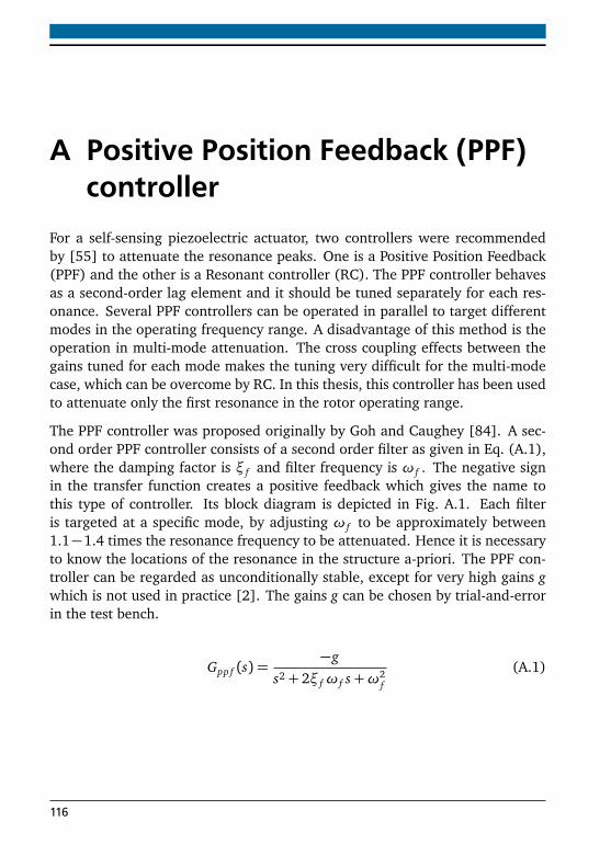
A Positive Position Feedback (PPF)controller

For a self-sensing piezoelectric actuator, two controllers were recommendedby [55] to attenuate the resonance peaks. One is a Positive Position Feedback(PPF) and the other is a Resonant controller (RC). The PPF controller behavesas a second-order lag element and it should be tuned separately for each res-onance. Several PPF controllers can be operated in parallel to target differentmodes in the operating frequency range. A disadvantage of this method is theoperation in multi-mode attenuation. The cross coupling effects between thegains tuned for each mode makes the tuning very difficult for the multi-modecase, which can be overcome by RC. In this thesis, this controller has been usedto attenuate only the first resonance in the rotor operating range.

The PPF controller was proposed originally by Goh and Caughey [84]. A sec-ond order PPF controller consists of a second order filter as given in Eq. (A.1),where the damping factor is ξ f and filter frequency is ω f . The negative signin the transfer function creates a positive feedback which gives the name tothis type of controller. Its block diagram is depicted in Fig. A.1. Each filteris targeted at a specific mode, by adjusting ω f to be approximately between1.1−1.4 times the resonance frequency to be attenuated. Hence it is necessaryto know the locations of the resonance in the structure a-priori. The PPF con-troller can be regarded as unconditionally stable, except for very high gains gwhich is not used in practice [2]. The gains g can be chosen by trial-and-errorin the test bench.

Gpp f (s) =−g

s2 + 2ξ fω f s+ω2f

(A.1)

116

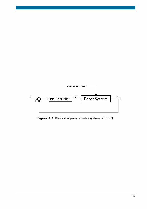
Figure A.1: Block diagram of rotorsystem with PPF

117

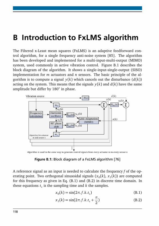
B Introduction to FxLMS algorithmThe Filtered x-Least mean squares (FxLMS) is an adaptive feedforward con-trol algorithm, for a single frequency anti-noise system [85]. The algorithmhas been developed and implemented for a multi-input-multi-output (MIMO)system, used commonly in active vibration control. Figure B.1 describes theblock diagram of the algorithm. It shows a single-input-single-output (SISO)implementation for m actuators and n sensors. The basic principle of the al-gorithm is to compute a signal y(k) which cancels out the disturbance (d(k))acting on the system. This means that the signals y(k) and d(k) have the sameamplitude but differ by 180 in phase.

Figure B.1: Block diagram of a FxLMS algorithm [76]

A reference signal as an input is needed to calculate the frequency f of the op-erating point. Two orthogonal sinusoidal signals (x0(k), x1(k)) are computedfor this frequency as given in Eq. (B.1) and (B.2) in discrete time domain. Inthese equations ts is the sampling time and k the samples.

x0(k) = sin(2π. f .k.ts) (B.1)

x1(k) = sin(2π. f .k.ts +π

2) (B.2)

118

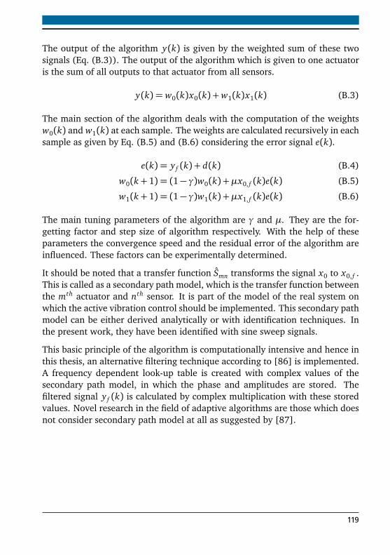
The output of the algorithm y(k) is given by the weighted sum of these twosignals (Eq. (B.3)). The output of the algorithm which is given to one actuatoris the sum of all outputs to that actuator from all sensors.

y(k) = w0(k)x0(k) +w1(k)x1(k) (B.3)

The main section of the algorithm deals with the computation of the weightsw0(k) and w1(k) at each sample. The weights are calculated recursively in eachsample as given by Eq. (B.5) and (B.6) considering the error signal e(k).

e(k) = y f (k) + d(k) (B.4)

w0(k+ 1) = (1− γ)w0(k) +µx0, f (k)e(k) (B.5)

w1(k+ 1) = (1− γ)w1(k) +µx1, f (k)e(k) (B.6)

The main tuning parameters of the algorithm are γ and µ. They are the for-getting factor and step size of algorithm respectively. With the help of theseparameters the convergence speed and the residual error of the algorithm areinfluenced. These factors can be experimentally determined.

It should be noted that a transfer function Smn transforms the signal x0 to x0, f .This is called as a secondary path model, which is the transfer function betweenthe mth actuator and nth sensor. It is part of the model of the real system onwhich the active vibration control should be implemented. This secondary pathmodel can be either derived analytically or with identification techniques. Inthe present work, they have been identified with sine sweep signals.

This basic principle of the algorithm is computationally intensive and hence inthis thesis, an alternative filtering technique according to [86] is implemented.A frequency dependent look-up table is created with complex values of thesecondary path model, in which the phase and amplitudes are stored. Thefiltered signal y f (k) is calculated by complex multiplication with these storedvalues. Novel research in the field of adaptive algorithms are those which doesnot consider secondary path model at all as suggested by [87].

119

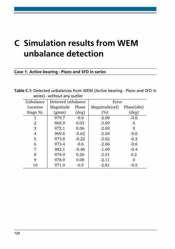
C Simulation results from WEMunbalance detection

Case 1: Active bearing - Piezo and SFD in series

Table C.1: Detected unbalances from WEM (Active bearing - Piezo and SFD inseries) - without any outlier

Unbalance Detected unbalance ErrorLocation Magnitude Phase Magnitude(rel) Phase(abs)Stage Nr. (gmm) (deg) (%) (deg)

1 979.7 -0.6 -2.09 -0.62 969.9 0.03 -3.09 03 972.1 0.06 -2.69 04 969.6 -0.62 -3.04 -0.65 973.8 -0.22 -2.62 -0.26 973.4 -0.6 -2.66 -0.67 983.1 -0.46 -1.69 -0.48 974.9 0.26 -2.51 0.29 978.9 0.08 -2.11 0

10 971.9 -0.5 -2.81 -0.5

120

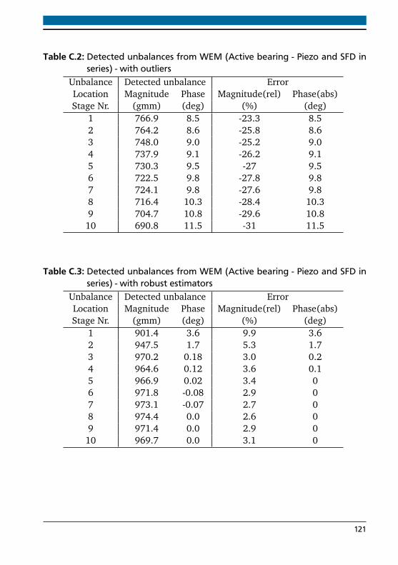
Table C.2: Detected unbalances from WEM (Active bearing - Piezo and SFD inseries) - with outliers

Unbalance Detected unbalance ErrorLocation Magnitude Phase Magnitude(rel) Phase(abs)Stage Nr. (gmm) (deg) (%) (deg)

1 766.9 8.5 -23.3 8.52 764.2 8.6 -25.8 8.63 748.0 9.0 -25.2 9.04 737.9 9.1 -26.2 9.15 730.3 9.5 -27 9.56 722.5 9.8 -27.8 9.87 724.1 9.8 -27.6 9.88 716.4 10.3 -28.4 10.39 704.7 10.8 -29.6 10.810 690.8 11.5 -31 11.5

Table C.3: Detected unbalances from WEM (Active bearing - Piezo and SFD inseries) - with robust estimators

Unbalance Detected unbalance ErrorLocation Magnitude Phase Magnitude(rel) Phase(abs)Stage Nr. (gmm) (deg) (%) (deg)

1 901.4 3.6 9.9 3.62 947.5 1.7 5.3 1.73 970.2 0.18 3.0 0.24 964.6 0.12 3.6 0.15 966.9 0.02 3.4 06 971.8 -0.08 2.9 07 973.1 -0.07 2.7 08 974.4 0.0 2.6 09 971.4 0.0 2.9 010 969.7 0.0 3.1 0

121

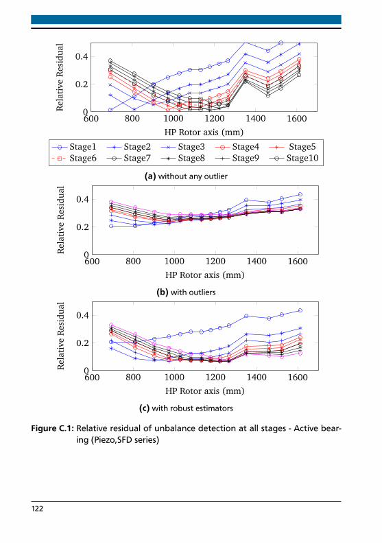
600 800 1000 1200 1400 16000

0.2

0.4

HP Rotor axis (mm)

Rel

ativ

eR

esid

ual

Stage1 Stage2 Stage3 Stage4 Stage5Stage6 Stage7 Stage8 Stage9 Stage10

(a) without any outlier

600 800 1000 1200 1400 16000

0.2

0.4

HP Rotor axis (mm)

Rel

ativ

eR

esid

ual

(b) with outliers

600 800 1000 1200 1400 16000

0.2

0.4

HP Rotor axis (mm)

Rel

ativ

eR

esid

ual

(c) with robust estimators

Figure C.1: Relative residual of unbalance detection at all stages - Active bear-ing (Piezo,SFD series)

122

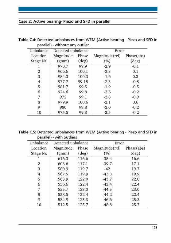
Case 2: Active bearing- Piezo and SFD in parallel

Table C.4: Detected unbalances from WEM (Active bearing - Piezo and SFD inparallel) - without any outlier

Unbalance Detected unbalance ErrorLocation Magnitude Phase Magnitude(rel) Phase(abs)Stage Nr. (gmm) (deg) (%) (deg)

1 970.7 99.9 -2.9 -0.12 966.6 100.1 -3.3 0.13 984.3 100.3 -1.6 0.34 977.7 99.18 -2.3 -0.85 981.7 99.5 -1.9 -0.56 974.6 99.8 -2.6 -0.27 972 99.1 -2.8 -0.98 979.9 100.6 -2.1 0.69 980 99.8 -2.0 -0.210 975.5 99.8 -2.5 -0.2

Table C.5: Detected unbalances from WEM (Active bearing - Piezo and SFD inparallel) - with outliers

Unbalance Detected unbalance ErrorLocation Magnitude Phase Magnitude(rel) Phase(abs)Stage Nr. (gmm) (deg) (%) (deg)

1 616.3 116.6 -38.4 16.62 603.6 117.1 -39.7 17.13 580.9 119.7 -42 19.74 567.5 119.9 -43.3 19.95 563.9 122.0 -43.7 22.06 556.6 122.4 -43.4 22.47 555.7 123.0 -44.5 23.08 558.5 122.4 -44.2 22.49 534.9 125.3 -46.6 25.310 512.5 125.7 -48.8 25.7

123

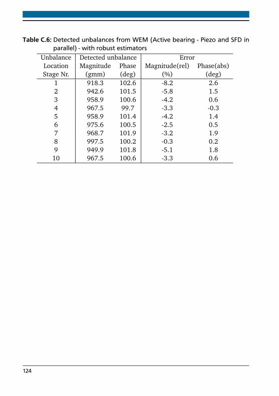
Table C.6: Detected unbalances from WEM (Active bearing - Piezo and SFD inparallel) - with robust estimators

Unbalance Detected unbalance ErrorLocation Magnitude Phase Magnitude(rel) Phase(abs)Stage Nr. (gmm) (deg) (%) (deg)

1 918.3 102.6 -8.2 2.62 942.6 101.5 -5.8 1.53 958.9 100.6 -4.2 0.64 967.5 99.7 -3.3 -0.35 958.9 101.4 -4.2 1.46 975.6 100.5 -2.5 0.57 968.7 101.9 -3.2 1.98 997.5 100.2 -0.3 0.29 949.9 101.8 -5.1 1.8

10 967.5 100.6 -3.3 0.6

124

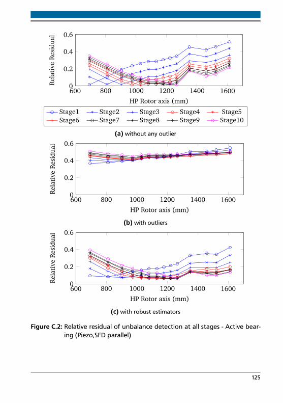
600 800 1000 1200 1400 16000

0.2

0.4

0.6

HP Rotor axis (mm)

Rel

ativ

eR

esid

ual

Stage1 Stage2 Stage3 Stage4 Stage5Stage6 Stage7 Stage8 Stage9 Stage10

(a) without any outlier

600 800 1000 1200 1400 16000

0.2

0.4

0.6

HP Rotor axis (mm)

Rel

ativ

eR

esid

ual

(b) with outliers

600 800 1000 1200 1400 16000

0.2

0.4

0.6

HP Rotor axis (mm)

Rel

ativ

eR

esid

ual

(c) with robust estimators

Figure C.2: Relative residual of unbalance detection at all stages - Active bear-ing (Piezo,SFD parallel)

125

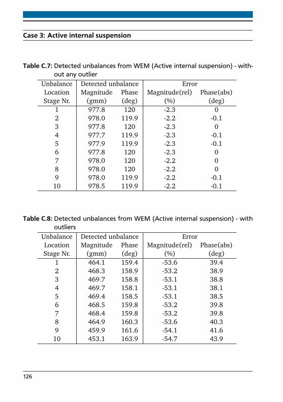
Case 3: Active internal suspension

Table C.7: Detected unbalances from WEM (Active internal suspension) - with-out any outlier

Unbalance Detected unbalance ErrorLocation Magnitude Phase Magnitude(rel) Phase(abs)Stage Nr. (gmm) (deg) (%) (deg)

1 977.8 120 -2.3 02 978.0 119.9 -2.2 -0.13 977.8 120 -2.3 04 977.7 119.9 -2.3 -0.15 977.9 119.9 -2.3 -0.16 977.8 120 -2.3 07 978.0 120 -2.2 08 978.0 120 -2.2 09 978.0 119.9 -2.2 -0.1

10 978.5 119.9 -2.2 -0.1

Table C.8: Detected unbalances from WEM (Active internal suspension) - withoutliers

Unbalance Detected unbalance ErrorLocation Magnitude Phase Magnitude(rel) Phase(abs)Stage Nr. (gmm) (deg) (%) (deg)

1 464.1 159.4 -53.6 39.42 468.3 158.9 -53.2 38.93 469.7 158.8 -53.1 38.84 469.7 158.1 -53.1 38.15 469.4 158.5 -53.1 38.56 468.5 159.8 -53.2 39.87 468.4 159.8 -53.2 39.88 464.9 160.3 -53.6 40.39 459.9 161.6 -54.1 41.6

10 453.1 163.9 -54.7 43.9

126

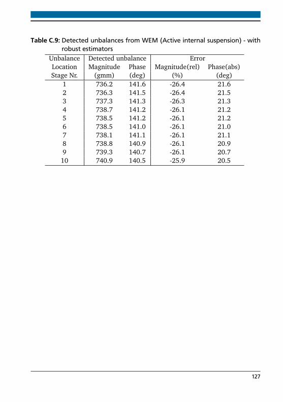
Table C.9: Detected unbalances from WEM (Active internal suspension) - withrobust estimators

Unbalance Detected unbalance ErrorLocation Magnitude Phase Magnitude(rel) Phase(abs)Stage Nr. (gmm) (deg) (%) (deg)

1 736.2 141.6 -26.4 21.62 736.3 141.5 -26.4 21.53 737.3 141.3 -26.3 21.34 738.7 141.2 -26.1 21.25 738.5 141.2 -26.1 21.26 738.5 141.0 -26.1 21.07 738.1 141.1 -26.1 21.18 738.8 140.9 -26.1 20.99 739.3 140.7 -26.1 20.710 740.9 140.5 -25.9 20.5

127

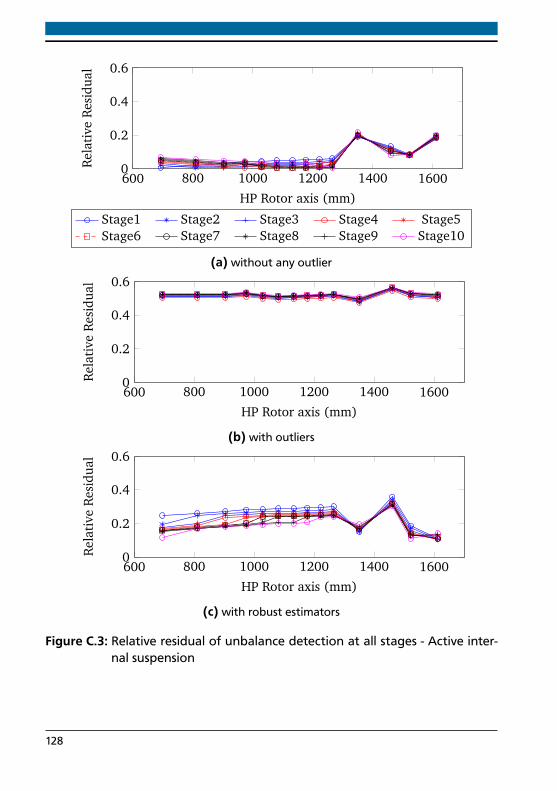
600 800 1000 1200 1400 16000

0.2

0.4

0.6

HP Rotor axis (mm)

Rel

ativ

eR

esid

ual

Stage1 Stage2 Stage3 Stage4 Stage5Stage6 Stage7 Stage8 Stage9 Stage10

(a) without any outlier

600 800 1000 1200 1400 16000

0.2

0.4

0.6

HP Rotor axis (mm)

Rel

ativ

eR

esid

ual

(b) with outliers

600 800 1000 1200 1400 16000

0.2

0.4

0.6

HP Rotor axis (mm)

Rel

ativ

eR

esid

ual

(c) with robust estimators

Figure C.3: Relative residual of unbalance detection at all stages - Active inter-nal suspension

128

Curriculum Vitae

Personal Ramakrishnan Ambur Sankaranarayananborn on 16. July 1987in Tirunelveli, India.

Studies1991 - 2004 School education

A.V.Rm.V Matriculation Higher Secondary School,Ambasamudram, India.

2004 - 2008 B.E.(Hons.) Mechanical EngineeringBirla Institute of Technology and Science, PilaniGoa campus, India.

2009 - 2012 M.Sc. Automotive EngineeringRWTH Aachen University, Germany.

2013 - 2016 PhD at Institute for Mechatronic Systems in Mechanical En-gineering,Technische Universität Darmstadt, Germany.

Job2008 - 2009 Trainee Engineer

Mercedes-Benz Research and Development India,Bengaluru, India.

129