Model Based Control of Air and EGR into a Diesel Engine

Master of Science Thesis HELENA ANDERSSON MARTIN HEDVALL Department of Signals and Systems Division of Automatic Control, Automation and Mechatronics CHALMERS UNIVERSITY OF TECHNOLOGY Göteborg, Sweden, 2008 Report No. EX005/2008

Exhaust gasInlet air

EGR cooler

Charge air cooler

VGT

EGR valve

MASTER OF SCIENCE THESIS EX005/2008

Model Based Control of Air and EGR into a Diesel Engine Helena Andersson Martin Hedvall

Supervisor: Johan Bengtsson, Hans Bernler Volvo Powertrain AB, Göteborg Examiner: Bo Egardt Chalmers University of Technology, Göteborg Department of Signals and Systems Division of Automatic Control, Automation and Mechatronics CHALMERS UNIVERSITY OF TECHNOLOGY Göteborg, Sweden, 2008

ii

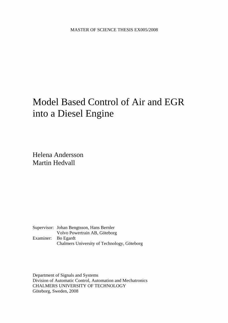
Model Based Control of Air and EGR into a Diesel Engine Master of Science Thesis Helena Andersson Martin Hedvall © 2008 by Helena Andersson and Martin Hedvall. Report No. EX005/2008 Department of Signals and Systems Division of Automatic Control, Automation and Mechatronics Chalmers University of Technology SE-412 96 Göteborg Sweden Telephone + 46 (0)31-772 1000 Performed in cooperation with Volvo Powertrain AB, Department 91535, Göteborg Supervisor: Johan Bengtsson and Hans Bernler, Volvo Powertrain AB, Göteborg Examiner: Bo Egardt, Chalmers University of Technology, Göteborg Cover: Schematic picture of gas and air flow in a modern diesel engine, see page 6. Chalmers Reproservice Göteborg, Sweden 2008

iii

Abstract Model Based Control of Air and EGR into a Diesel Engine Helena Andersson Martin Hedvall Department of Signals and Systems Division of Automatic Control, Automation and Mechatronics Chalmers University of Technology Due to environmental pollution, the automotive industry is forced to meet with lowered emission demands legislated by the government. Improved technologies for engine control are essential. The use of a Variable Geometry Turbine (VGT) and Exhaust Gas Recirculation (EGR) can make the fulfilment of the emission demands possible. The purpose of this thesis was to control the VGT and the EGR valve with a multivariable controller. Such a controller was necessary in order to handle cross coupling effects between control signals and output signals. Several model based linear controllers were used to handle the nonlinear behaviour of the VGT and the EGR valve. Dynamic data was crucial for the model design in order to describe the complex behaviour of the actuators, with adequate accuracy. The measurements in this thesis were performed on a 13 litre Volvo diesel engine with a VGT and a short EGR route implementation. System identification was used to estimate models for the control purpose. These models consisted of fourth order subspace models. An LQG-controller was used in order to control an engine model. The investigated control design consisted of a proportional controller, both with and without additional integral action implemented. The results of simulations with these designs, made it clear that feed forward of measurable disturbance signals was essential for an acceptable control. Two different interpolation methods were used in order to go from one state-space model to another. The best control design was achieved with an LQG-controller with feed forward, additional integral action and a linear fraction based interpolation strategy. Keywords: model based control, VGT, EGR, linear models, LQG

iv

v

Acknowledgements There are a number of people who have contributed to this master thesis and we owe our thanks to them all. First of all we would like to thank Johan Bengtsson and Hans Bernler, our supervisors at Volvo Powertrain AB, for genuine guiding and support during the whole project. We also owe our many thanks to Per-Olof Källén, Volvo Powertrain AB, for always taking time to discuss the assignment with us and showing interest in the task. We would also like to thank Bo Egardt, our examiner at Chalmers University of Technology, for giving lots of useful inputs. Many thanks will also be directed towards the staff at the department of 91535 at Volvo Powertrain AB, for a warm welcome and acceptance. In a random order we would like to send our gratitude to; Lars Antbäck, Ingemar Gustafsson, Lars Johansson, Alistair Low, Moataz Ali, Kent Johnsson, Patrik Persson, Mikael Bengtsson, Göran Axbrink, Andreas Nilsson, Matilda Törngren and Mikael Karlsson. We are grateful for the support, encouragement and patience of our families throughout the process. Helena would especially like to thank Erik for always being there for her, as well as her parents, Gerd and Karl-Eric and her sister Veronika. Martin would also like to thank Linda for her great way of backing him up, as well as his parents Eva and Kjell and his sister Anna.

Helena Andersson Martin Hedvall

February 2008, Göteborg

vi

vii

Table of Contents

1 Introduction............................................................................................................. 1 1.1 Background and purpose .................................................................................. 1 1.2 Problem analysis............................................................................................... 2

1.2.1 The measurement problem ....................................................................... 2 1.2.2 The modelling problem ............................................................................ 2 1.2.3 The control problem ................................................................................. 2

1.3 Method and limitations..................................................................................... 2 1.4 Disposition........................................................................................................ 3

2 Description of VGT and EGR Valve ........................................................................ 5 2.1 The Variable Geometry Turbine....................................................................... 5 2.2 Exhaust Gas Re-circulation .............................................................................. 6

3 System Identification Theory ................................................................................. 7 3.1 Experiment design ............................................................................................ 7 3.2 Data processing................................................................................................. 8 3.3 Model estimation .............................................................................................. 8

3.3.1 ARX models ............................................................................................. 9 3.3.2 State-space models using a subspace method .......................................... 9

3.4 Model validation............................................................................................. 10 3.4.1 Stability analysis and pole-zero cancellation.......................................... 11 3.4.2 Residual analysis .................................................................................... 11

4 Control Theory....................................................................................................... 13 4.1 Linear Quadratic control................................................................................. 13 4.2 Kalman filter design ....................................................................................... 14 4.3 Implementation of additional integral action ................................................. 15 4.4 Feed forward of additional input signals ........................................................ 16

5 Measurements and Data Processing.................................................................. 19 5.1 Design of engine test experiment ................................................................... 19 5.2 Measurements in engine test cell.................................................................... 21

viii

6 Model Estimation and Validation ........................................................................ 23 6.1 Model design and parameter estimation......................................................... 23 6.2 Model validation............................................................................................. 24

6.2.1 Verification of model behaviour............................................................. 24 6.2.2 Stability check and pole zero cancellation ............................................. 26 6.2.3 Model residual analysis .......................................................................... 27

6.3 Merging of models ......................................................................................... 29

7 The Combined Engine Model ............................................................................... 35 7.1 Design of the combined engine model using linear interpolation.................. 35

7.1.1 Fraction based interpolation method ...................................................... 35 7.1.2 Time and fraction based interpolation method....................................... 36

7.2 Validation of engine model switch behavior.................................................. 36

8 Implementation of Control Design ...................................................................... 41 8.1 Control algorithm ........................................................................................... 41

8.1.1 Kalman filter design ............................................................................... 41 8.1.2 Implementation of basic LQG-control ................................................... 43 8.1.3 Stability margins of the closed loop system ........................................... 43 8.1.4 Implementation of additional integral action ......................................... 44 8.1.5 Implementation of feed forward............................................................. 45 8.1.6 Implementation of time constants in the feed forward of the reference

signals ..................................................................................................... 46 8.2 Interpolation strategy between control models............................................... 47

8.2.1 Time based interpolation method ........................................................... 48 8.2.2 Fraction based interpolation method ...................................................... 48

9 Validation of Control Algorithm using the Combined Engine Model ................. 49 9.1 Interpolation strategies for control models..................................................... 49

9.1.1 Time based interpolation method ........................................................... 50 9.1.2 Fraction based interpolation method ...................................................... 52

9.2 Validation of merged control models ............................................................. 54 9.3 LQG-control with feed forward...................................................................... 57 9.4 LQG-control with feed forward and additional integral action..................... 58

10 Discussion ............................................................................................................. 61 10.1 Measurements and modeling.......................................................................... 61 10.2 The Combined engine model.......................................................................... 62 10.3 Control design ................................................................................................ 62 10.4 Validation of control algorithm on engine model .......................................... 63 10.5 Future work .................................................................................................... 63

11 Conclusions........................................................................................................... 65

Bibliography ................................................................................................................... 67

A System Identification Validation .......................................................................... 69 A.1 Different orders of ARX models .................................................................... 69

ix

A.2 Pole zero visualization.................................................................................... 71 A.3 Residual analysis ............................................................................................ 72 A.4 Merging of models ......................................................................................... 73

B Control design validation .................................................................................... 75

x

xi

Abbreviations Abbreviation Description ARX Auto-Regression with eXtra inputs ECU Engine Control Unit EGR Exhaust Gas Recirculation EMS Engine Management System LQ Linear Quadratic LQG Linear Quadratic Gaussian MIMO Multiple-Input Multiple-Output VGT Variable Geometry Turbine

xii

1

1 Introduction

This chapter gives an introduction to the subject of the master thesis and also a description of its purpose. Problem formulation, methods and limitations of the task are found in this part, as well as disposition of the thesis. 1.1 Background and purpose Due to global warming effects and environmental pollution, a lot of attention has been focused on the automotive industry. Emissions from diesel engines have been a common topic in the climate debate. The heavy duty industry is therefore forced to meet with lower emission demands legislated by the government. In order to fulfil these harsh demands, improved technologies for engine control are crucial. Such techniques that make it possible to fulfil these restrictions are EGR and the use of a VGT. When the exhaust gas is re-circulated back into the engine, NOx emissions are reduced. The EGR rate also influences the particle matter formation and the fuel consumption of the engine. As NOx is reduced through EGR, more particles are formed due to deteriorated combustion. A trade-off between NOx and soot has to be made in order to fulfil legislation standards. Air and EGR flow into the engine have to be controlled during both stationary and transient conditions in order to fulfil the demands of low emissions and fuel consumption. The two actuators used to control air and EGR flow into the engine are the VGT and the EGR valve. A change in the VGT position will affect both the EGR rate and the amount of air into the engine. In a similar way a change in the EGR valve position affects both inlets to the engine. During transients the behaviour is even more complex, especially since the exhaust pressure is not measured in a production engine. The characteristics of the actuators are also very nonlinear and depend on the working conditions of the engine. A more detailed description of the VGT and EGR is found in Chapter 2. The purpose of this master thesis was to control air and EGR flow into a diesel engine during both stationary and transient behaviour. A set of linear model based controllers was used for this mission.

2

1.2 Problem analysis The work in this thesis has been divided into three different parts. The first part consists of measurements made in engine test cell and data analysis. In the second part modelling work performed on data from an engine test cell is addressed. Finally, the third part concerns the actual VGT and EGR control. 1.2.1 The measurement problem Dynamic data was needed in order to design models describing the complex behaviour of the VGT and the EGR valve. Therefore, a test experiment had to be prepared in order to run an engine in a test cell. Data collection was made with a number of different VGT and EGR valve positions for a set of different speed and torque combinations in the areas of interest. 1.2.2 The modelling problem Models were necessary when designing model based controllers for the system. The main issue was to design as few linear models as possible describing the nonlinear behaviour of the VGT and EGR valve with sufficient accuracy. The purpose was to develop a method that needed as little data from an engine test cell as possible and was easy to implement and optimize. The estimated models are dynamical multivariable models. 1.2.3 The control problem The aim was to use the parameter settings developed from modelling to design a set of linear controllers. Given a specific working point, the VGT and EGR actuators were to be controlled in order to reach the desired reference values. 1.3 Method and limitations This project has been carried out as follows:

• A literature survey was made on the VGT and the EGR valve. Also, a study of system identification and control theory was performed.

• Experiments for data collection were thoroughly designed and carried out.

• Data was analyzed and linear models were identified and represented as state-

space models. The tool used for identifying models was System Identification Toolbox in MATLAB.

• Control algorithms were designed and implemented in MATLAB/SIMULINK.

3

• Preliminary sets of state-space models were evaluated with control algorithms. The work with model design was performed in parallel to control design.

• The chosen set of models was implemented in the final control design and

evaluated on a modelled engine. Some limitations had to be made in order to agree with the time aspect of the project as well as the complexity of the task.

• The system identification theory only concentrates on ARX models and subspace models using a subspace method. This decision was made in order to limit the number of different model estimations.

• Due to problems finding a proper engine model for simulation matters, the

engine operating region was dramatically restrained. 1.4 Disposition The outline of every chapter in this thesis is based on the same principles as the work has been executed in, please refer to Section 1.2.

• Chapter 2 includes an overview of the VGT and EGR and their function.

• Chapter 3 gives the theory for system identification and model evaluation.

• Chapter 4 describes the theory for control design and control loops are graphically visualized.

• Chapter 5 explains how engine test experiments for transient data collection are

designed and further on in the chapter it is also described how data from measurements are processed.

• Chapter 6 describes the work of model estimation and validation made on data

from measurements. • Chapter 7 includes information about the engine model used for simulation.

• Chapter 8 describes the implemented control algorithm in SIMULINK.

• Chapter 9 includes how validation of the control design in the engine model is

made and analyzed. • Chapter 10 includes a discussion about the results presented in the previous

chapters. • Chapter 11 gives the conclusions made in this thesis.

4

5

2 Description of VGT and EGR Valve

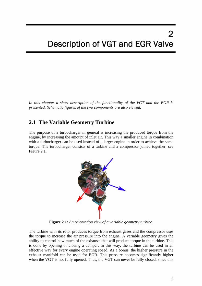
In this chapter a short description of the functionality of the VGT and the EGR is presented. Schematic figures of the two components are also viewed. 2.1 The Variable Geometry Turbine The purpose of a turbocharger in general is increasing the produced torque from the engine, by increasing the amount of inlet air. This way a smaller engine in combination with a turbocharger can be used instead of a larger engine in order to achieve the same torque. The turbocharger consists of a turbine and a compressor joined together, see Figure 2.1.

Figure 2.1: An orientation view of a variable geometry turbine.

The turbine with its rotor produces torque from exhaust gases and the compressor uses the torque to increase the air pressure into the engine. A variable geometry gives the ability to control how much of the exhausts that will produce torque in the turbine. This is done by opening or closing a damper. In this way, the turbine can be used in an effective way for every engine operating speed. As a bonus, the higher pressure in the exhaust manifold can be used for EGR. This pressure becomes significantly higher when the VGT is not fully opened. Thus, the VGT can never be fully closed, since this

6

totally blocks the exhaust gases from leaving the engine. The behaviour of the VGT is strongly nonlinear due to its vanes in the damper. The vanes do not have a uniform shape and therefore the area, through which the exhaust gases flow, changes in a nonlinear way. As a consequence of this, the exhaust manifold pressure has a very nonlinear behaviour. A change in the VGT position affects the pressure more when the VGT is almost closed, than when it is fully opened. 2.2 Exhaust Gas Re-circulation EGR is a way of re-circulating exhaust gases back into the cylinders. The purpose of this is reducing the NOx emissions from the engine. NOx particles are created at high temperatures when oxygen is available. The exhaust gases contain almost no oxygen compared to fresh air. Replacing fresh air with exhaust gases means less oxygen to the cylinders. The amount of exhaust gases that are re-circulated is controlled by a valve, see Figure 2.2. The valve has a nonlinear behaviour, but not as nonlinear as the VGT. The nonlinearity originates from the construction of the valve. A very small valve opening means that the gases can only flow through a small area of the pipe. By opening the valve just slightly, the flow area increases considerably. The shape of the valve gives rise to a significantly higher flow difference for a small change of the valve in the almost closed region, than changing the valve position the same distance in a more opened one. This effect originates from the fact that the EGR flow becomes saturated. The valve also causes whirls in the gases that flow through it, which contributes to the nonlinearity. These whirls appear when the gas leaves the valve, and enters a space with a bigger cross section area.

Figure 2.2: Schematic picture of gas and air flow in a modern diesel engine. Figure 2.2 describes a short EGR route configuration, where gas is re-circulated from the exhaust manifold and passed through a cooler. To make the EGR process work, the pressure in the exhaust manifold must be higher than the pressure in the intake manifold. Without a VGT, this happens only at short time intervals, at the same instant as the exhaust gases are being pushed out of the cylinders. Since a VGT gives the possibility to build up a higher pressure in the exhaust manifold, EGR can be used to a greater extent.

7

3 System Identification Theory

Theories and methods for experiment design, data processing, model estimation and validation are presented in this chapter. System identification is the powerful way of identifying data in order to estimate a useful model. The procedure for this work can be summarized in Figure 3.1.

Data

Data

Model

Yes

Bad

dat

a

B

ad m

odel

stru

ctur

e

Figure 3.1: The circle of system identification.

3.1 Experiment design The design of a system identification experiment includes many important choices. First the designer has to decide which signals to measure. Inputs and outputs for the system have to be considered thoroughly. When these have been defined the next issue is to

8

decide the sampling frequency. The rate is determined from the dynamic properties in the input and output signals. To be able to identify this behaviour, the sampling rate has to be fast enough to get all the wanted dynamics, but not so fast as to generate unnecessarily large amounts of data. 3.2 Data processing When data is collected from experiment, immediate usages in identification algorithms are often not possible. First the data has to be pre-processed in several ways in order to eliminate low- and high-frequency disturbances, outliers, missing data, drifts and offsets etc. Removal of offsets such as drifts and trends are especially important when output error models are used as estimation output. If this is not considered, difference in amplitude will dominate the fit criterion and the dynamic behaviour will be of less importance. For methods that use flexible noise models, removal of offsets is not as crucial, since this approach, by design, means de-emphasis of drifts and trends. One such method is the least-squares method, see Ljung (1999). The data measurement equipment is not faultless. Therefore, the data will most likely include bad values due to obvious measurement error. Such data are called outliers. These types of values may have negative effect on the estimate and it is recommended to remove such data from the experiment. Residual analysis is good for identifying outliers and bad data. For further reading, see Ljung (1999). As discussed earlier in this section, bad data might be included in measurements and other data might be missing for any reason. One reason to merge data sets might be that an experiment has been repeated for a number of times and it is desired to design only one model, based on the data from all experiments. Whatever the reason might be, it is desired to exclude parts of bad data and concatenate other parts. As good as it might sound; it is not possible to simply connect data segments together, since the joining points would cause transient behaviour that might destroy the estimate. Therefore merging data sets can be done with statistical methods, using covariance matrices. For more details about how this is done, see Ljung (1999) and The MATLAB Users Guide (2006). 3.3 Model estimation There are a number of different model structures to choose between when describing a system. First the user has to decide upon whether to use linear or nonlinear models, black-box or physically parameterized state-space models etc. In this master thesis the focus is to design linear models for MIMO systems. Not all model structures can handle multivariable systems. ARX models and state-space models using a subspace method are two models useful for this purpose.

9

3.3.1 ARX models A discrete multivariable ARX model with nu inputs and ny outputs is described by (3.1).

( ) [ ] ( ) [ ] [ ]kenkkuqBkyqA +−= (3.1) A(q) is an ny-by-ny matrix whose entries are polynomials in the delay operator q-1, B(q) is an ny-by-nu matrix and e[k] is white noise, see (3.2).

( )

( )⎪⎩

⎪⎨

⎧

+++=

+++=

−−

−−

nbnb

nanany

qBqBBqB

qAqAIqA

...

...

110

11

(3.2)

e

Figure 3.2: The ARX model structure.

Figure 3.2 gives a graphical description of (3.1). Hence, the number of parameters in the A(q) or B(q) polynomials increases with higher orders, i.e. na and nb. The delay from input to output is determined by nk. Parameters are estimated using the linear least squares method. For further reading, see Ljung and Glad (2004) and The MATLAB Users Guide (2006). The ARX model is the simplest model to estimate due to its estimation algorithm. For this reason, it is preferred to try ARX models as a first attempt to estimate a model structure. The disadvantages with using an ARX model, is that the noise model is described using the same poles as the rest of the system, see (3.1). Higher orders of the A and B polynomials might therefore be needed, which is not of such big importance for good signal-to-noise conditions. For references, see Ljung and Glad (2004). Note that an ARX model has to be transformed into a state-space model, before implementation in the control algorithm intended for use in this thesis, see (3.3) for a state-space representation. 3.3.2 State-space models using a subspace method Mathematically, a discrete state-space model is described by (3.3). Measured inputs sampled at time k are denoted as u and outputs as y. The number of inputs is nu and the number of outputs is ny. The vector x is the state vector and contains numerical values of n states. w and v are immeasurable signals, assumed to be white noise.

10

[ ] [ ] [ ] [ ]

[ ] [ ] [ ] [ ]⎪⎩

⎪⎨

⎧

++=

++=+

kvkuDkxCky

kwkuBkxAkx 1 (3.3)

In (3.3) A is an n-by-n matrix, which describes the dynamics of the system. B is an n-by-nu matrix and it describes the linear transformation by which the inputs influence the next state. C is an ny-by-n matrix, which represents how the internal state is transferred to the output y. D is an ny-by-nu matrix, which is the direct feed through term. Complex behaviour in the measured outputs can be captured by choosing n high enough in the model estimation. For further reading, see van Overschee and De Moor (1996). In Figure 3.3 a graphical representation of a state-space model is made.

v w

Figure 3.3: The state-space model structure.

Subspace identification algorithms identify input-state-output models. If the states of the system are known and input and output data are measured, it would be possible to solve (3.3) for the four matrices. The equation would be a linear regression and the C and D matrices can be found by applying the least squares method. Hence, the other unknown matrices in the equation can then be determined. The problem is thus to find the states. In (3.3) the states can be described as linear combinations of the k-step-ahead predicted output. Once these predictors are found the problem is solved. This can be achieved by using a subspace method. These methods determine the predictors by projections directly on the measured data sequences in a satisfactory way. For more details, see Ljung (1999). Unlike ARX models, subspace models have full freedom in the noise model. Therefore, a lower order can be used for subspace models compared to ARX models. Subspace models are also very easy to implement in control algorithms, since the system matrices are directly known. 3.4 Model validation Model validation is made in order to determine if an estimated model is good enough for describing certain behaviour. The validation part of the system identification process is of big importance for finding an estimated model with good qualifications.

11

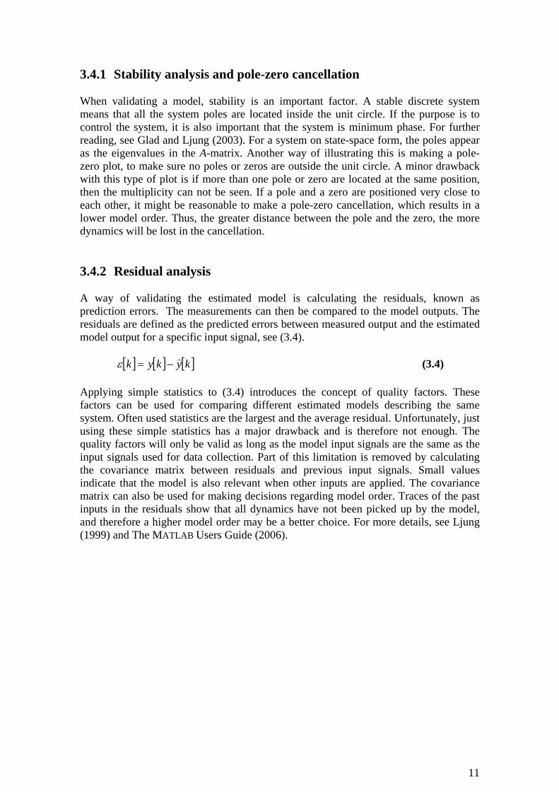
3.4.1 Stability analysis and pole-zero cancellation When validating a model, stability is an important factor. A stable discrete system means that all the system poles are located inside the unit circle. If the purpose is to control the system, it is also important that the system is minimum phase. For further reading, see Glad and Ljung (2003). For a system on state-space form, the poles appear as the eigenvalues in the A-matrix. Another way of illustrating this is making a pole-zero plot, to make sure no poles or zeros are outside the unit circle. A minor drawback with this type of plot is if more than one pole or zero are located at the same position, then the multiplicity can not be seen. If a pole and a zero are positioned very close to each other, it might be reasonable to make a pole-zero cancellation, which results in a lower model order. Thus, the greater distance between the pole and the zero, the more dynamics will be lost in the cancellation.

3.4.2 Residual analysis A way of validating the estimated model is calculating the residuals, known as prediction errors. The measurements can then be compared to the model outputs. The residuals are defined as the predicted errors between measured output and the estimated model output for a specific input signal, see (3.4).

[ ] [ ] [ ]kykyk )−=ε (3.4)

Applying simple statistics to (3.4) introduces the concept of quality factors. These factors can be used for comparing different estimated models describing the same system. Often used statistics are the largest and the average residual. Unfortunately, just using these simple statistics has a major drawback and is therefore not enough. The quality factors will only be valid as long as the model input signals are the same as the input signals used for data collection. Part of this limitation is removed by calculating the covariance matrix between residuals and previous input signals. Small values indicate that the model is also relevant when other inputs are applied. The covariance matrix can also be used for making decisions regarding model order. Traces of the past inputs in the residuals show that all dynamics have not been picked up by the model, and therefore a higher model order may be a better choice. For more details, see Ljung (1999) and The MATLAB Users Guide (2006).

12

13

4 Control Theory

In this Chapter theories and methods for control design are presented. The control design described in this chapter utilizes a multivariable optimal linear control theory; LQG with additional integral action and feed forward. 4.1 Linear Quadratic control A multivariable controller is needed in order to control cross dependent signals simultaneously. It is especially important if the signals have essential cross coupling effects on each other. The LQ-control strategy uses negative feedback of the system states in order to create control signals. Since it is a model based controller, the system to be controlled must be represented as a state space model, see Section 3.3.2 and (3.3). It is also required that the pair (A,B) is stabilizable and that the pair (A,Q) is detectable. Q is to be explained in the next section. For further reading, see Glad and Ljung (2003). The LQ-control problem consists of minimizing a loss function, denoted J. This loss function includes the control signals and the system states, see Åström and Wittenmark (1997). The loss function also includes adjustable parameters, Q and R, which gives the possibility to put weights on each state and each control signal, see (4.1). It is also possible to put weights on the cross coupling effects between states and/or control signals. For example, small weights on control signals would give fast control, however the control signal activity would be high.

( ) ( ) ( ) ( ) ( ) ( ) ( )( )∑=

++∞→

=k

n

TTT nuRnunuNnxnxQnxkk

kJ0

1lim (4.1)

( ) ( )kxLku −= (4.2)

Applying (4.2) to (4.1) and minimizing the resulting equation will give the optimal gain matrix L. From this, together with the negative feedback of the states, the control law can be calculated.

14

In order to follow a given reference vector, the reference signals must be included in the control law, see (4.3).

( ) ( ) ( )kxLkrLku r −= (4.3) In (4.3), Lr is a gain matrix that ensures the static gain of the closed system is equal to one. The controller is now able to reach the desired references, assuming that the state space model is perfectly describing the real system. See Figure 4.1 for a schematic picture of the control setup.

Figure 4.1: Visualization of a system controlled by an LQ-controller.

In Figure 4.1 the inputs, the outputs and the control signals can be either scalars or vectors with an arbitrary number of elements. 4.2 Kalman filter design In order to implement a model based controller for a system, all states in the model must be known. If the number of states differs from the number of measured outputs, the states cannot be directly calculated. Thus, an observer is necessary to predict states. A Kalman filter has been proved to give an optimal balance between the sensitivity to measurement noise and the prediction of states. For more details, see Glad and Ljung (2003). The covariance matrices for the process disturbances, denoted R1, and for the measurement noise, denoted R2, are adjustable parameters. All known noise behaviour should be included in these parameters in order to perform a good prediction. There is also an adjustable matrix for the cross coupling effects between the process disturbances and the measurement noise, denoted R12. The Kalman filter requires that the matrix R2 is symmetric and that the matrix TRRRRR 12

121211

~ −−= is positive definite. It also requires that (A,C) is detectable and that ( 1

1212

~, RCRRA −− ) is stabilizable. The Kalman matrix K is then calculated by solving the Riccati equation, in which all mentioned covariance matrices are included, see Glad and Ljung (2003). The predicted states are calculated by solving the state-space model in (4.4). A schematic picture of the control setup with the Kalman estimator is seen in Figure 4.2.

( ) ( ) ( ) ( ) ( )( )

( ) ( ) ( )⎪⎩

⎪⎨

⎧

+=

−++=+

kuDkxCky

kxCkyKkuBkxAkx

ˆˆ

ˆˆ1ˆ (4.4)

15

Figure 4.2: Visualization of a system controlled by an LQG-controller.

As seen in Figure 4.2, the Kalman filter uses both control signals and output signals from the system to make a good prediction of the states. 4.3 Implementation of additional integral action A model can never be a perfect match of a real system. One reason is that disturbances and measurement noise will affect the measurements. Therefore, an LQ-controller will result in stationary errors in the system output signals. The amplitude of the errors depends on how much the model differs from the real system. Implementing additional integral action to the controller solves this problem. In practice, this is carried out by adding integrator states, which become part of the control signal, see (4.3) and (4.5). Thus, the control signal will change until the control error is zero. One extra state for each output signal is therefore needed. For further reading, see Schmidtbauer (1999).

( ) ( ) ( ) ( )kykrkxkx −+=+ intint 1 (4.5)

Adding integral states results in an increased state space model, see (4.6). See also Figure 4.3 for a schematic figure of the control setup.

( )( )

( )( )

( )( )( )

( ) [ ] ( )( )

( ) [ ] ( )( ) [ ]

( )( )( )⎪

⎪⎪⎪⎪

⎩

⎪⎪⎪⎪⎪

⎨

⎧

⎥⎥⎥

⎦

⎤

⎢⎢⎢

⎣

⎡+⎥

⎦

⎤⎢⎣

⎡=

⎟⎟⎠

⎞⎜⎜⎝

⎛⎥⎦

⎤⎢⎣

⎡−+

⎥⎥⎥

⎦

⎤

⎢⎢⎢

⎣

⎡

⎥⎦

⎤⎢⎣

⎡−

+⎥⎦

⎤⎢⎣

⎡⎥⎦

⎤⎢⎣

⎡=⎥

⎦

⎤⎢⎣

⎡++

kykrku

Dkx

kxCky

kxkx

CkyKkykrku

IIB

kxkx

IA

kxkx

00ˆ

0ˆ

ˆ0

000ˆ

00

11ˆ

int

intintint

(4.6)

The optimal gain matrix must be recalculated minimizing the loss function again, with the integral states added.

16

Figure 4.3: Visualization of a system controlled by an LQG-controller with additional

integral action. Due to (4.6), the inputs to the Kalman estimator have to be augmented with the reference vector, when implementing additional integral action. 4.4 Feed forward of additional input signals Integral action compensates for stationary errors in the output signals, but on the other hand integral action is relatively slow. If the controlled system has measurable disturbances, feed forward of these signals will give rise to a faster controlling. The simplest way of doing this is multiplying the disturbance signals with a static gain matrix, denoted Lff in Figure 4.4. This matrix should be designed in such way that the control signal contribution from feed forward will compensate for the model output contribution from the disturbance signals. The static gain matrix is received by solving (4.7) if Guy is a square matrix with a determinant different from zero.

( ) ( ) ( ) ( ) 000 =+ kvGkvLG vyffuy (4.7)

Applying the static gain matrix from (4.7) in (4.8) gives the total control signal u from both feedback and feed forward.

( ) ( ) ( ) ( )( )⎥⎦

⎤⎢⎣

⎡−+=

kxkx

LkvLkrLku ffrint

ˆ (4.8)

v(k) is a vector including all the additional inputs, and Lff is the gain matrix.

17

Systemy

L

u

Kalmanfilter

x

xint

rLr

Lffv

^

+ -

+

Figure 4.4: Visualization of a system controlled by an LQG-controller with additional

integral action and feed forward. Since the feed forward is free from dynamics and directly operates on the control signals, the control speed of the system increases dramatically.

18

19

5 Measurements and Data Processing

This chapter gives a description of how the test experiments for measurement collection in an engine test cell are designed and how data are processed. The measurements are performed on a 13 litre Volvo diesel engine with a VGT and a short EGR route implementation. 5.1 Design of engine test experiment Since the controller should be able to produce satisfactory control signals, data from transient driving conditions for the engine had to be used. A diesel engine can not run with any random combinations of VGT and EGR valve positions. Therefore, each driving condition must be carefully selected. Dynamic data needed for model and control design had not been measured. For that reason a transient engine test experiment had to be designed. From static measurements, it was possible to find proper combinations of VGT and EGR valve positions for different speeds and loads. Both the VGT and the EGR valve have nonlinear behaviour in some regions. In these regions the actuators can not be adjusted too rapidly in order to get all dynamic information. To avoid turbo over-speeding the VGT also has a lower limit for each operating point. Three different engine speeds were chosen and two different loads for each speed in order to design the engine test sequences. The combinations of load and engine speed are common operating points for the type of engine used in the experiment. For each of the combinations, the VGT and the EGR valve positions have been varied within acceptable operating ranges, see Figure 5.1.

20

0 0.5 1 1.5 2 2.5 3

x 104

1000

1500

2000

2500

Time [s]

Torq

ue [N

m],

Spee

d [r

pm]

TorqueSpeed

0 0.5 1 1.5 2 2.5 3

x 104

0

50

100

Time [s]

VG

T [%

], EG

R [%

]

VGTEGR

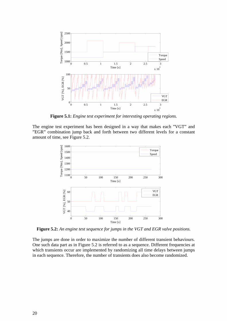
Figure 5.1: Engine test experiment for interesting operating regions.

The engine test experiment has been designed in a way that makes each ”VGT” and ”EGR” combination jump back and forth between two different levels for a constant amount of time, see Figure 5.2.

0 50 100 150 200 250 3001100

1200

1300

1400

1500

1600

Time [s]

Torq

ue [N

m],

Spee

d [r

pm]

TorqueSpeed

0 50 100 150 200 250 300

40

50

60

Time [s]

VG

T [%

], EG

R [%

]

VGTEGR

Figure 5.2: An engine test sequence for jumps in the VGT and EGR valve positions.

The jumps are done in order to maximize the number of different transient behaviours. One such data part as in Figure 5.2 is referred to as a sequence. Different frequencies at which transients occur are implemented by randomizing all time delays between jumps in each sequence. Therefore, the number of transients does also become randomized.

21

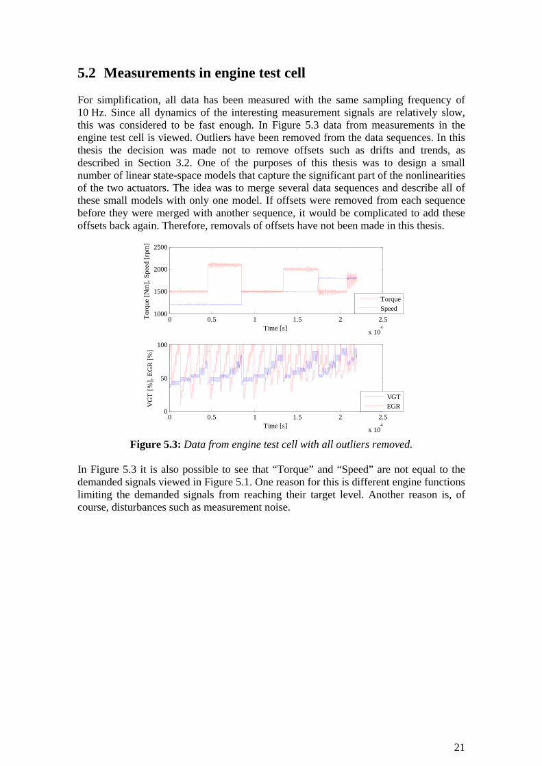
5.2 Measurements in engine test cell For simplification, all data has been measured with the same sampling frequency of 10 Hz. Since all dynamics of the interesting measurement signals are relatively slow, this was considered to be fast enough. In Figure 5.3 data from measurements in the engine test cell is viewed. Outliers have been removed from the data sequences. In this thesis the decision was made not to remove offsets such as drifts and trends, as described in Section 3.2. One of the purposes of this thesis was to design a small number of linear state-space models that capture the significant part of the nonlinearities of the two actuators. The idea was to merge several data sequences and describe all of these small models with only one model. If offsets were removed from each sequence before they were merged with another sequence, it would be complicated to add these offsets back again. Therefore, removals of offsets have not been made in this thesis.

0 0.5 1 1.5 2 2.5

x 104

1000

1500

2000

2500

Time [s]

Torq

ue [N

m],

Spee

d [r

pm]

TorqueSpeed

0 0.5 1 1.5 2 2.5

x 104

0

50

100

Time [s]

VG

T [%

], EG

R [%

]

VGTEGR

Figure 5.3: Data from engine test cell with all outliers removed.

In Figure 5.3 it is also possible to see that “Torque” and “Speed” are not equal to the demanded signals viewed in Figure 5.1. One reason for this is different engine functions limiting the demanded signals from reaching their target level. Another reason is, of course, disturbances such as measurement noise.

22

0 0.5 1 1.5 2 2.5

x 104

0

5

10

15

20

Time [s]EG

R co

nten

t [%

]

0 0.5 1 1.5 2 2.5

x 104

100

200

300

400

Time [s]

Boos

t pre

ssur

e [k

Pa]

Figure 5.4: Two measured data signals used for model estimation from engine test cell,

outliers are removed. In Figure 5.4 two measured data signals, ”EGR content” and ”Boost pressure”, are shown. The output signals in this figure are a result from the engine test cell, where the engine have been run with the input signals shown in Figure 5.3. These two signals have been used for model estimation since they are proportional to NOx and soot, and thus give a good indication of the emission levels. The “EGR content” is defined as a relative measure of the EGR amount in the inlet manifold.

23

6 Model Estimation and Validation

This chapter presents the results of system identification modelling using different methods and model parameters. In the first section the model design and parameter estimation is addressed. After that, the models are validated in various steps according to Section 6.2. In the last section merged models are examined. 6.1 Model design and parameter estimation Since both the VGT and the EGR valve have nonlinear behaviour, it appeared to be too hard to predict any optimal model order directly from using their physics. In order to get satisfactory results, some different model orders were tested and the model that best described the reality was chosen. To determine the best model; model errors, time delays and model overshoots were considered. Different model orders were tested for both ARX and subspace models. The number of different transient behaviours that can occur for one data sequence was quite small. Also, the working region for one data sequence was very narrow and the behaviour of the “EGR content” and the “Boost pressure” was expected to be linear. Therefore, a fairly low order linear model was reasonable to expect as the best one. For ARX models, the time delay could be found using the trial and error method. With this method, the time delay nk was determined to be equal to one. In contrast to ARX models, the time delays for subspace models were estimated automatically by the subspace method. Therefore, only one parameter, the model order n, had to be adjusted in order to find an optimal model. For ARX models, both na and nb remained adjustable after the time delay was found. The measurement data and ranges for input signals used for model estimation are shown in Table 6.1. Even though more measurement data was obtained, see Section 5.2, this is the only data used for model estimation presented in this thesis. This is due to problems in finding a proper engine model, further discussed in Section 10.2.

24

Model 1 Model 2 Model 3 Model 4

Original data sequence 1 2 3 4 Number of samples 1400 1375 1100 1549 Speed [rpm] 1200 1200 1200 1200 Torque [Nm] 1500 1500 1500 1500 VGT range [%] 40-45 40-45 45-50 45-50 EGR range [%] 50-60 60-70 50-60 60-70

Table 6.1: Measurement data used for model estimation.

The accuracy of the model estimation depending on “Speed” and “Torque” is unreliable; as only disturbances have contributed to the output dynamics, see Figure 5.3. 6.2 Model validation Each estimated model was validated in order to find the best one for the control purpose. Since an ARX model produced a worse output than a subspace model with the same number of states, this master thesis will focus on subspace models. ARX models contributed to a high number of states even for low order models. 6.2.1 Verification of model behaviour

In order to make sure that the significant dynamics have been captured by the model, verification has been performed. Thus, the model behaviour was compared to the physical reality using MATLAB. The influence of the model order was investigated using a trial and error method, by starting off with a low order model and increasing the order step by step until the most reasonable output signals were reached. A fourth order subspace model was found to be the best one. Results from some ARX models can be found in Appendix A.1.

0 20 40 60 80 100 120 1405

10

15

20

EGR

cont

ent [

%]

Time [s]

0 20 40 60 80 100 120 140240

245

250

255

260

Boos

t pre

ssur

e [k

Pa]

Time [s]

Measured outputModel output

Measured outputModel output

Figure 6.1: A first order subspace model compared with data from measurements.

25

It is clear that great parts of the dynamic behaviour were lost during the estimation of a first order subspace model, see Figure 6.1. Especially the model output of the ”EGR content” lost almost all dynamics and even got a non physical behaviour at some operating regions.

0 20 40 60 80 100 120 1406

8

10

12

EGR

cont

ent [

%]

Time [s]

0 20 40 60 80 100 120 140240

245

250

255

260

Boos

t pre

ssur

e [k

Pa]

Time [s]

Measured outputModel output

Measured outputModel output

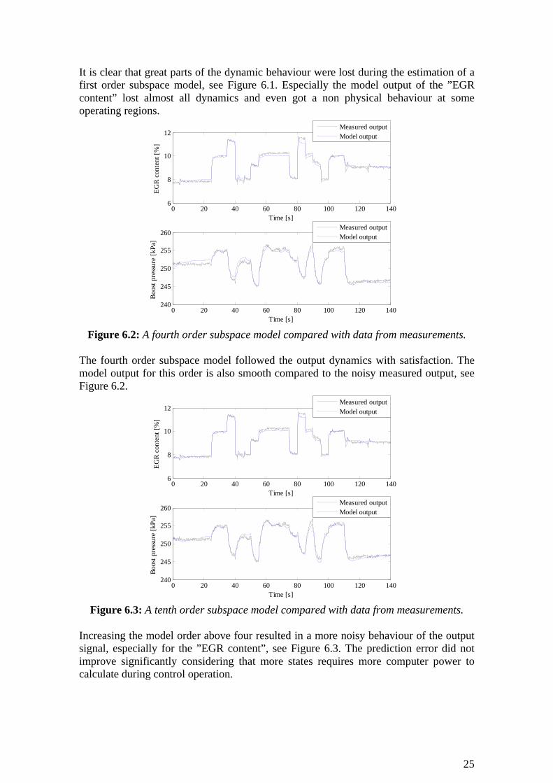
Figure 6.2: A fourth order subspace model compared with data from measurements.

The fourth order subspace model followed the output dynamics with satisfaction. The model output for this order is also smooth compared to the noisy measured output, see Figure 6.2.

0 20 40 60 80 100 120 1406

8

10

12

EGR

cont

ent [

%]

Time [s]

0 20 40 60 80 100 120 140240

245

250

255

260

Boos

t pre

ssur

e [k

Pa]

Time [s]

Measured outputModel output

Measured outputModel output

Figure 6.3: A tenth order subspace model compared with data from measurements.

Increasing the model order above four resulted in a more noisy behaviour of the output signal, especially for the ”EGR content”, see Figure 6.3. The prediction error did not improve significantly considering that more states requires more computer power to calculate during control operation.

26

6.2.2 Stability check and pole zero cancellation The stability of all models was tested since this is crucial for a model based control system. In this test, all absolute distances between the origin and the poles and zeros were calculated. The calculation revealed the stability of the models and whether the models were minimum phase or not. To be able to do a proper stability check, each model has been split into two different two-by-two transfer functions, one from the “Speed” and “Torque” signals to the output signals and one from the control signals to the output signals. See Figure 6.4 and Figure 6.5 for visualization of the system poles and zeros for a fourth order subspace model. Similar figures for an ARX model are found in Appendix A.2.

-1 -0.8 -0.6 -0.4 -0.2 0 0.2 0.4 0.6 0.8 1-1

-0.8

-0.6

-0.4

-0.2

0

0.2

0.4

0.6

0.8

1

Re

Im

Zeros in transfer function from Speed and Torque to outputsPoles in transfer function from Speed and Torque to outputs

Figure 6.4: Pole-zero visualization of the multidimensional transfer function from “Speed” and “Torque” to ”EGR content” and ”Boost pressure” for a fourth order

subspace model. In Figure 6.4, some poles are located close to the boundary of the unit circle, but the distance calculation based on eigenvalues revealed that all poles are stable. The distance calculation for the zeros exposed that the system was minimum phase.

27

-1 -0.8 -0.6 -0.4 -0.2 0 0.2 0.4 0.6 0.8 1-1

-0.8

-0.6

-0.4

-0.2

0

0.2

0.4

0.6

0.8

1

Re

Im

Zeros in transfer function from VGT and EGR to outputsPoles in transfer function from VGT and EGR to outputs

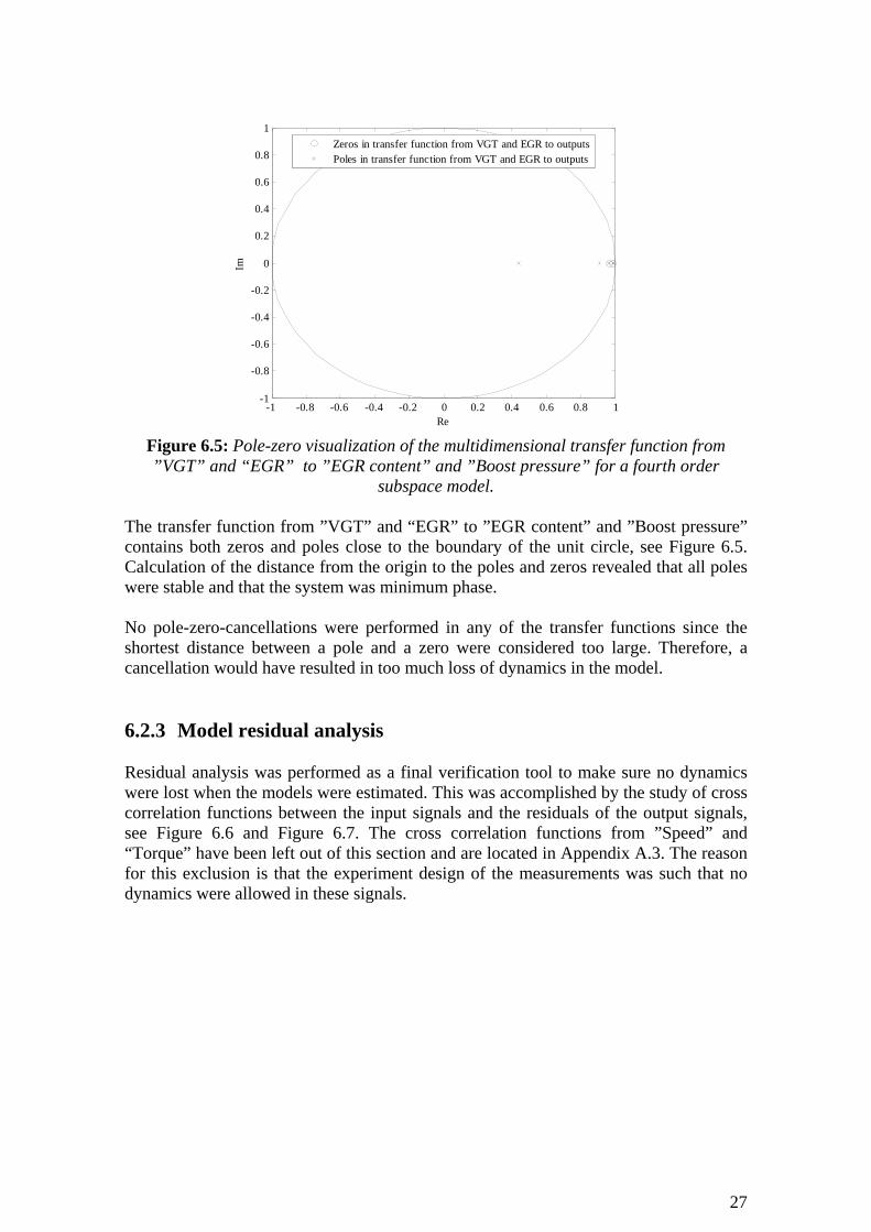
Figure 6.5: Pole-zero visualization of the multidimensional transfer function from ”VGT” and “EGR” to ”EGR content” and ”Boost pressure” for a fourth order

subspace model. The transfer function from ”VGT” and “EGR” to ”EGR content” and ”Boost pressure” contains both zeros and poles close to the boundary of the unit circle, see Figure 6.5. Calculation of the distance from the origin to the poles and zeros revealed that all poles were stable and that the system was minimum phase. No pole-zero-cancellations were performed in any of the transfer functions since the shortest distance between a pole and a zero were considered too large. Therefore, a cancellation would have resulted in too much loss of dynamics in the model. 6.2.3 Model residual analysis Residual analysis was performed as a final verification tool to make sure no dynamics were lost when the models were estimated. This was accomplished by the study of cross correlation functions between the input signals and the residuals of the output signals, see Figure 6.6 and Figure 6.7. The cross correlation functions from ”Speed” and “Torque” have been left out of this section and are located in Appendix A.3. The reason for this exclusion is that the experiment design of the measurements was such that no dynamics were allowed in these signals.

28

-2.5 -2 -1.5 -1 -0.5 0 0.5 1 1.5 2 2.5-0.2

-0.1

0

0.1

0.2

Time lag [s]

Cros

s cor

rela

tion

-2.5 -2 -1.5 -1 -0.5 0 0.5 1 1.5 2 2.5-0.2

-0.1

0

0.1

0.2

Time lag [s]

Cros

s cor

rela

tion

99% confidence intervalCross correlation between EGR and residuals from EGR content

99% confidence intervalCross correlation between VGT and residuals from EGR content

Figure 6.6: Cross correlation functions between “VGT” and “EGR” inputs and

residuals from ”EGR content” for a fourth order subspace model. In Figure 6.6, the correlation function is consistently very close to zero. Therefore, it becomes clear that all relevant influences on ”EGR content” from ”VGT” and “EGR” inputs have been captured by the model. Refer to Section 3.4.2 for theory regarding covariance between input signals and output residuals.

-2.5 -2 -1.5 -1 -0.5 0 0.5 1 1.5 2 2.5-0.1

-0.05

0

0.05

0.1

Time lag [s]

Cros

s cor

rela

tion

-2.5 -2 -1.5 -1 -0.5 0 0.5 1 1.5 2 2.5-0.1

-0.05

0

0.05

0.1

Time lag [s]

Cros

s cor

rela

tion

99% confidence intervalCross correlation between EGR and residuals from Boost pressure

99% confidence intervalCross correlation between VGT and residuals from Boost pressure

Figure 6.7: Cross correlation functions between ”VGT” and “EGR” inputs and

residuals from ”Boost pressure” for a fourth order subspace model. Figure 6.7 reveals that all relevant influence on ”Boost pressure” from “VGT” and “EGR” has been captured by the model also.

29

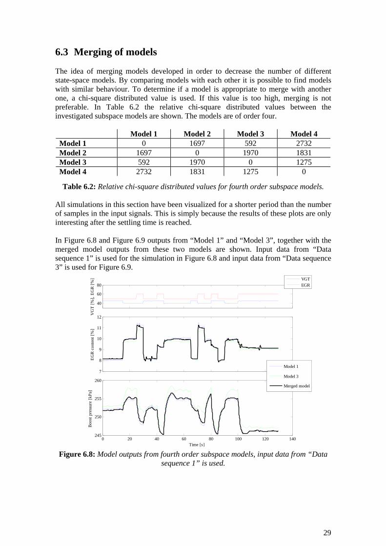
6.3 Merging of models The idea of merging models developed in order to decrease the number of different state-space models. By comparing models with each other it is possible to find models with similar behaviour. To determine if a model is appropriate to merge with another one, a chi-square distributed value is used. If this value is too high, merging is not preferable. In Table 6.2 the relative chi-square distributed values between the investigated subspace models are shown. The models are of order four.

Model 1 Model 2 Model 3 Model 4 Model 1 0 1697 592 2732 Model 2 1697 0 1970 1831 Model 3 592 1970 0 1275 Model 4 2732 1831 1275 0

Table 6.2: Relative chi-square distributed values for fourth order subspace models.

All simulations in this section have been visualized for a shorter period than the number of samples in the input signals. This is simply because the results of these plots are only interesting after the settling time is reached. In Figure 6.8 and Figure 6.9 outputs from “Model 1” and “Model 3”, together with the merged model outputs from these two models are shown. Input data from “Data sequence 1” is used for the simulation in Figure 6.8 and input data from “Data sequence 3” is used for Figure 6.9.

40

60

80

VG

T [%

], EG

R [%

]

VGTEGR

7

8

9

10

11

12

EGR

cont

ent [

%]

0 20 40 60 80 100 120 140245

250

255

260

Time [s]

Boos

t pre

ssur

e [k

Pa]

Model 1

Model 3

Merged model

Figure 6.8: Model outputs from fourth order subspace models, input data from “Data

sequence 1” is used.

30

40

60

80

VG

T [%

], EG

R [%

]

VGTEGR

5

6

7

8

9

10

EGR

cont

ent [

%]

0 20 40 60 80 100 120240

245

250

255

Time [s]

Boos

t pre

ssur

e [k

Pa]

Model 1

Model 3

Merged model

Figure 6.9: Model outputs from fourth order subspace models, input data from “Data

sequence 3” is used.

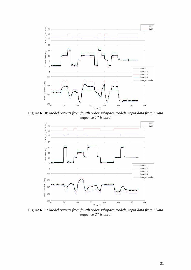
In Figure 6.8 the merged model outputs are supposed to have the same behaviour as the outputs from “Model 1”. This is seen in the figure; both outputs seem to follow the behaviour acceptably well. In Figure 6.9 the merged model is supposed to generate outputs with the same appearance as “Model 3”. This is also verified in the figure. The merged model of “Data sequence 1” and “Data sequence 2” has the lowest chi-square distributed value in Table 6.2. From the analysis of the two figures it is seen that a merge between these two data sequences is preferable. All four data sequences that have been used for simulation of the control loop have also been merged together as one model. Visualizations of this are shown in Figure 6.10 to Figure 6.13. The input data for the model estimates have been varied in the four figures. The input data in Figure 6.10 are from “Data sequence 1”, in Figure 6.11 from “Data sequence 2”, in Figure 6.12 from “Data sequence 3” and in Figure 6.13 from “Data sequence 4”.

31

40

60

80

VG

T [%

], EG

R [%

]

VGTEGR

7

8

9

10

11

12EG

R co

nten

t [%

]

0 20 40 60 80 100 120 140245

250

255

260

Time [s]

Boos

t pre

ssur

e [k

Pa]

Model 1Model 2Model 3Model 4Merged model

Figure 6.10: Model outputs from fourth order subspace models, input data from “Data

sequence 1” is used.

40

60

80

VG

T [%

], EG

R [%

]

VGTEGR

8

9

10

11

12

13

EGR

cont

ent [

%]

0 20 40 60 80 100 120 140235

240

245

250

255

Time [s]

Boos

t pre

ssur

e [k

Pa]

Model 1Model 2Model 3Model 4Merged model

Figure 6.11: Model outputs from fourth order subspace models, input data from “Data

sequence 2” is used.

32

40

60

80

VG

T [%

], EG

R [%

]

VGTEGR

5

6

7

8

9

10EG

R co

nten

t [%

]

0 20 40 60 80 100 120240

245

250

255

Time [s]

Boos

t pre

ssur

e [k

Pa]

Model 1Model 2Model 3Model 4Merged model

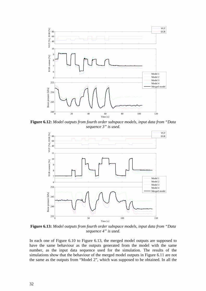
Figure 6.12: Model outputs from fourth order subspace models, input data from “Data

sequence 3” is used.

40

60

80

VG

T [%

], EG

R [%

]

VGTEGR

6

7

8

9

10

11

EGR

cont

ent [

%]

0 50 100 150235

240

245

250

Time [s]

Boos

t pre

ssur

e [k

Pa]

Model 1Model 2Model 3Model 4Merged model

Figure 6.13: Model outputs from fourth order subspace models, input data from “Data

sequence 4” is used. In each one of Figure 6.10 to Figure 6.13, the merged model outputs are supposed to have the same behaviour as the outputs generated from the model with the same number, as the input data sequence used for the simulation. The results of the simulations show that the behaviour of the merged model outputs in Figure 6.11 are not the same as the outputs from “Model 2”, which was supposed to be obtained. In all the

33

other figures, the aimed behaviour is considered to be within acceptable margins. Hence, merging of all four data sequences might not be preferable. To further investigate if merging of models is appropriate, it is recommended to study the appearance of Bode diagrams. If the appearance of both the amplitude and the phase are about the same for the models intended to merge, then merging is preferable. In Figure 6.14 and Figure 6.15 the Bode plots for outputs from “Model 1”, “Model 3” and a merged model of these two are shown. Figure 6.14 visualizes the Bode diagram of the transfer function from ”VGT” to the model outputs, whilst Figure 6.15 shows the transfer function from “EGR” to the outputs instead. Analogous Bode diagrams for ”Speed” and “Torque” are found in Appendix A.4

10-3

10-2

10-1

100

101

102

10-2

10-1

100

Am

plitu

de

Frequency [rad/s]

10-3

10-2

10-1

100

101

102

0

50

100

150

200

Phas

e [d

eg]

Frequency [rad/s]

Frequency response from Model 1Frequency response from Model 3Frequency response from Merged model

10-3

10-2

10-1

100

101

102

10-2

10-1

100

Am

plitu

de

Frequency [rad/s]

10-3

10-2

10-1

100

101

102

0

50

100

150

200

Phas

e [d

eg]

Frequency [rad/s]

Frequency response from Model 1Frequency response from Model 3Frequency response from Merged model

Figure 6.14: Bode diagram of the transfer function from ”VGT” to ”EGR content” (left) and ”Boost pressure” (right). The plots are for outputs from “Model 1” and

“Model 3”, together with a merged model, for fourth order estimates.

10-3

10-2

10-1

100

101

102

10-2

10-1

100

Am

plitu

de

Frequency [rad/s]

10-3

10-2

10-1

100

101

102

-200

-100

0

100

Phas

e [d

eg]

Frequency [rad/s]

Frequency response from Model 1Frequency response from Model 3Frequency response from Merged model

10-3

10-2

10-1

100

101

102

10-3

10-2

10-1

100

Am

plitu

de

Frequency [rad/s]

10-3

10-2

10-1

100

101

102

-100

0

100

200

Phas

e [d

eg]

Frequency [rad/s]

Frequency response from Model 1Frequency response from Model 3Frequency response from Merged model

Figure 6.15: Bode diagram of the transfer function from “EGR” to burned fraction (left) and ”Boost pressure” (right). The plots are for outputs from “Model 1” and

“Model 3”, together with a merged model, for fourth order estimates. In Figure 6.14 and Figure 6.15 it is seen that the frequency response have the same appearance for both models and also the merged model. Since the sampling frequency was 10 Hz, it is only relevant to compare the behaviour for frequencies under 5 Hz. 5 Hz is half the sampling frequency, which is also the same as the Nyquist frequency. The figures also confirm that merging of “Model 1” and “Model 3” is beneficial.

34

35

7 The Combined Engine Model

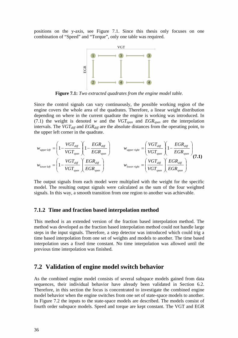
In this chapter a description of the combined engine model used for simulation is given. First, a description of the model design is presented and secondly, a validation of the combined engine model is made. 7.1 Design of the combined engine model using linear

interpolation When designing the combined engine model, the aspiration was to obtain a model that was as similar to the real engine as possible. This means a huge number of state-space models were needed in order to describe the complete engine. Only six different speed and torque combinations were examined when data was obtained in the engine test cell. Such a small number of different working areas would be inadequate to describe the total engine. Therefore, such a realization was unachievable and the limitation was made to focus on merely a very small working region. That region is defined by the state-space models estimated from the data sequences in Table 6.1. Thus, no data sequences are merged together since this would impair the result. The combined engine model consists of a maximum of four different state-space models. 7.1.1 Fraction based interpolation method When implementation of the state-space models were made in SIMULINK, a strategy to choose the proper model was necessary. Linear interpolation was used to smoothly go from the output signals of one set of state-space models to another. Depending on speed, torque, VGT and EGR valve positions, the most suitable state-space models were selected. A four dimensional look-up system was therefore required. The interpolation strategy was such that four state-space models were always selected. The four models represent corners in a quadrate. Each quadrate represents a very small working area in the VGT and EGR valve position regions for a fixed combination of “Speed” and “Torque”. All quadrates that represent the same “Speed” and “Torque” combination were merged together in a table, with VGT positions on the x-axis and EGR valve

36

positions on the y-axis, see Figure 7.1. Since this thesis only focuses on one combination of “Speed” and “Torque”, only one table was required.

1 3

2 4

3

4

VGT

EGR

Figure 7.1: Two extracted quadrates from the engine model table.

Since the control signals can vary continuously, the possible working region of the engine covers the whole area of the quadrates. Therefore, a linear weight distribution depending on where in the current quadrate the engine is working was introduced. In (7.1) the weight is denoted w and the VGTspan and EGRspan are the interpolation intervals. The VGTdiff and EGRdiff are the absolute distances from the operating point, to the upper left corner in the quadrate.

⎟⎟⎠

⎞⎜⎜⎝

⎛⎟⎟⎠

⎞⎜⎜⎝

⎛=⎟

⎟⎠

⎞⎜⎜⎝

⎛⎟⎟⎠

⎞⎜⎜⎝

⎛−=

⎟⎟⎠

⎞⎜⎜⎝

⎛−⎟

⎟⎠

⎞⎜⎜⎝

⎛=⎟

⎟⎠

⎞⎜⎜⎝

⎛−⎟

⎟⎠

⎞⎜⎜⎝

⎛−=

span

diff

span

diffrightlower

span

diff

span

diffleftlower

span

diff

span

diffrightupper

span

diff

span

diffleftupper

EGREGR

VGTVGT

wEGREGR

VGTVGT

w

EGREGR

VGTVGT

wEGREGR

VGTVGT

w

1

111

(7.1)

The output signals from each model were multiplied with the weight for the specific model. The resulting output signals were calculated as the sum of the four weighted signals. In this way, a smooth transition from one region to another was achievable. 7.1.2 Time and fraction based interpolation method This method is an extended version of the fraction based interpolation method. The method was developed as the fraction based interpolation method could not handle large steps in the input signals. Therefore, a step detector was introduced which could trig a time based interpolation from one set of weights and models to another. The time based interpolation uses a fixed time constant. No time interpolation was allowed until the previous time interpolation was finished. 7.2 Validation of engine model switch behavior As the combined engine model consists of several subspace models gained from data sequences, their individual behavior have already been validated in Section 6.2. Therefore, in this section the focus is concentrated to investigate the combined engine model behavior when the engine switches from one set of state-space models to another. In Figure 7.2 the inputs to the state-space models are described. The models consist of fourth order subspace models. Speed and torque are kept constant. The VGT and EGR

37

valve positions are kept constant at three different levels and are ramped in between. All input signals are in the operating range for at least one subspace model at all times. This thesis focuses on the fraction based interpolation method for the engine. Though, a comparison between the two different methods is found in the end of this section. The simulations visualized in Figure 7.2 to Figure 7.5 use the fraction based interpolation method.

0 5 10 15 20 25 30 35 40

1200

1300

1400

1500

Time [s]

Torq

ue [N

m],

Spee

d [r

pm]

TorqueSpeed

0 5 10 15 20 25 30 35 40

40

50

60

70

Time [s]

VG

T [%

], EG

R [%

]

VGTEGR

Figure 7.2: Input signals for fourth order state-space models.

In Figure 7.3 the output signals from the combined engine model are visualized. From the figure it is possible to see the smoothness in the outputs resulting from changes in the inputs and the interpolation strategy.

0 5 10 15 20 25 30 357

8

9

10

11

EGR

cont

ent [

%]

Time [s]

0 5 10 15 20 25 30 35235

240

245

250

255

Boos

t pre

ssur

e [k

Pa]

Time [s]

Figure 7.3: Output signals from the combined engine model.

The four subplots in Figure 7.4 represent the corners in the floating quadrate, found in the engine model table. In each subplot, one of the state-space models currently in use is shown and also a weight to indicate how much of its outputs that are used in the combined engine model. During the first 10 seconds the combined engine model is

38

based on only “Model 1”. After the first change in VGT and EGR valve position have occurred, the combined engine model consists of the maximum number of four different state-space models. As a consequence of the input signals, each model output is used with 25 percent at this period. The tweaks in the weight fraction after 10 and 21 seconds are a result from the interpolation strategy when the input signals are changed.

0

2

4

FractionModel

0

2

4M

odel

num

ber

FractionModel

0

2

4

Mod

el fr

actio

n,

FractionModel

0 5 10 15 20 25 30 350

2

4

Time [s]

FractionModel

Figure 7.4: Model numbers and weights for fourth order subspace models, each subplot

represents the corners in the floating quadrate, found in the engine model table. For the input signals shown in Figure 7.2, simulations have been done with only using one of the four subspace models at a time. The results from the four models are found in Figure 7.5. It is the output result from these individual models that have been interpolated. The outcome of the interpolation for the combined engine model depends on the weights and model numbers shown in Figure 7.4.

0 5 10 15 20 25 30 357

8

9

10

11

Time [s]

EGR

cont

ent [

%]

Model 1Model 2Model 3Model 4Combined model

0 5 10 15 20 25 30 35230

240

250

260

Time [s]

Boos

t pre

ssur

e [k

Pa]

Model 1Model 2Model 3Model 4Combined model

Figure 7.5: Output signals from fourth order subspace models.

39

Figure 7.6 shows a comparison between the two different interpolation methods described in Section 7.1. In order to do a relevant comparison, the first ramp in both control signals was replaced by a step; since the time based interpolation method needs to be triggered.

0 5 10 15 20 25 307

8

9

10

11

Time [s]

EGR

cont

ent [

%]

Fraction based interpolation methodTime and fraction based interpolation method

0 5 10 15 20 25 30235

240

245

250

255

Boos

t pre

ssur

e [k

Pa]

Time [s]

Figure 7.6: Comparison between different interpolation methods in the combined engine model.

As the fraction based interpolation method can not interpolate during steps in the input signals, a bump occurs when a step is applied. The time and fraction based interpolation method prevented this bump, but in trade, the control system is slightly slower. As the result from the two different interpolation methods in Figure 7.6 was similar, only the fraction based interpolation method was used in the validation of the control algorithm.

40

41

8 Implementation of Control Design

This chapter gives a deep presentation of the model based control design. All control designs in this chapter use a fourth order subspace model created from “Data sequence 1” for both the controller and the engine model. 8.1 Control algorithm A model based LQG-control design has been chosen in order to control the diesel engine. The choice was made since this type of linear controller can handle MIMO systems including cross coupling effects between the control signals and the outputs, see Section 4.1. This control design requires that all system states are known and therefore, a Kalman filter was implemented in order to predict the unknown states. The controller was also improved with additional integral action and feed forward of the “Speed” and “Torque” signals. Finally, the feed forward path was slightly slowed down using time constants in order to give smoother control signals. 8.1.1 Kalman filter design Each model created from the data sequences contains more states than system outputs and therefore, an observer had to be implemented in order to predict the states. The identified systems were observable. An optimal Kalman filter was used for the state prediction, see Section 4.2. The adjustable parameters in the R1 matrix were chosen to be smaller than the parameters in the R2 matrix, because measurement noise was expected to be larger than process disturbances from the engine. An assumption was made that no cross correlation between measurement noise and process disturbances existed, and therefore the matrix R12 was chosen to be zero. Since each model includes the input signals “Speed” and “Torque” in addition to the control signals, these signals had to be treated as measurable disturbances by the Kalman filter. If not, it would have been impossible to predict the states that depend on “Speed” and “Torque” correctly. See Figure 8.1 for a comparison between actual states and predicted states for a fourth order subspace model.

42

0 50 100 1504.7

4.8

4.9

5

Am

plitu

de

Time [s]

State 1, actualState 1, predicted

0 50 100 150

0.8

1

1.2

1.4

Am

plitu

de

Time [s]

State 2, actualState 2, predicted

24.8 24.9 254.84

4.845

4.85

4.855

4.86

Am

plitu

de

Time [s]

State 1, actualState 1, predicted

0 50 100 150-0.6

-0.4

-0.2

0

0.2

Am

plitu

de

Time [s]

State 3, actualState 3, predicted

0 50 100 150

5.85

5.9

5.95

6

Am

plitu

de

Time [s]

State 4, actualState 4, predicted

Figure 8.1: Visualization of all states for a fourth order subspace model together with

the Kalman predicted states. Figure 8.1 shows that the actual state curves are totally covered by the curves for the predicted states, therefore it is concluded that the observer works properly. In order to make sure that no mismatch in time delay has occurred, a zoomed part of the curves for “State 1” is visualized in the subplot to the right. The state prediction has also been tested with a disturbance added to the output signals. This resulted as expected in a slightly worse state prediction, but the Kalman filter adjusted the states in the correct direction, see Figure 8.2. The subplot to the right shows that no time delay exists between the predicted states and the actual states.

0 50 100 1504.7

4.8

4.9

5

Am

plitu

de

Time [s]

State 1, actualState 1, predicted

0 50 100 150

0.8

1

1.2

1.4

Am

plitu

de

Time [s]

State 2, actualState 2, predicted

24.8 24.9 254.84

4.845

4.85

4.855

4.86

Am

plitu

de

Time [s]

State 1, actualState 1, predicted

0 50 100 150-0.6

-0.4

-0.2

0

0.2

Am

plitu

de

Time [s]

State 3, actualState 3, predicted

0 50 100 150

5.85

5.9

5.95

6

Am

plitu

de

Time [s]

State 4, actualState 4, predicted

Figure 8.2: Visualization of all states for a fourth order subspace model, together with

states predicted from noisy output signals. The noise signal used in Figure 8.2 is normal distributed with zero mean and standard deviation equal to one. The output signals have different noise signals, but the same

43

distribution. The Kalman parameters used in this simulation were IR 2.01 = and IR 5.02 = .

8.1.2 Implementation of basic LQG-control The requirements for calculating the optimal gain matrix were fulfilled, since the matrix (A,B) was found to be stabilizable and the matrix (A,Q) was detectable. The weight parameters on the control signals were adjusted in order to receive a proper control signal contribution from the feedback. The goal was to approximately give the feedback the same order of magnitude as the contribution from the reference signals. However, without both additional integral action and feed forward of “Speed” and “Torque”, the requested output signals could not be followed correctly, see Figure 8.3.

0 20 40 60 80 100 120 1400

20

40

EGR

cont

ent [

%]

ActualDemanded

0 20 40 60 80 100 120 140200

400

600

Boos

t pre

ssur

e [k

Pa]

ActualDemanded

0 20 40 60 80 100 120 140-115

-110

-105

-100

VG

T [%

]

0 20 40 60 80 100 120 140-360

-340

-320

-300

EGR

[%]

Time [s] Figure 8.3: Output responses from steps in the reference signals for LQG-control of

“Model 1”. In Figure 8.3 it is clearly visible that the control signals have very non physical levels since feed forward of “Speed” and “Torque” is missing. Though, it is also clear that the controller works properly, since it reacts in the correct direction when steps are applied in the reference signals. 8.1.3 Stability margins of the closed loop system All models created from the data sequences were already found to be stable. The stability margins of each control setup were examined by calculating all poles for the closed loop system. The simulations confirmed that all poles were located within the unit circle, but not with too significant margins, see Figure 8.4.

44

-1 -0.8 -0.6 -0.4 -0.2 0 0.2 0.4 0.6 0.8 1-1

-0.8

-0.6

-0.4

-0.2

0

0.2

0.4

0.6

0.8

1

Re

Im

Poles in the closed loop system

Figure 8.4: Poles in the closed loop system for a fourth order subspace model.

8.1.4 Implementation of additional integral action In order to reach the desired reference signals, additional integral action was implemented. As the models have two control signals, two integral states were necessary to add. The increased amount of states required that the optimal gain matrix was increased with as many columns as added states. The new columns could not be chosen arbitrarily due to the cross coupling effects on the outputs from the control signals. Instead, the optimal gain matrix had to be recalculated for the increased number of states, in order to receive the new columns. The new optimal gain matrix could either be used directly, or the new columns could be extracted and inserted in the previous optimal gain matrix. This thesis includes both methods, but focuses on the second method. Implementing additional integral action using the second method required two different R and Q matrices with adjustable parameters. The matrices used without integral states are denoted as RNoInt and QNoInt and the matrices used with integral states included are denoted R and Q. The stationary errors in Figure 8.3 are very large and therefore a strong control signal contribution from the integral states was needed. Though, too much integral action made the closed loop system unstable. The contribution was adjusted by changing the relevant parameters in the Q matrix. Figure 8.5 shows the result from additional integral action applied to the controller described in 8.1.2.

45

0 20 40 60 80 100 120 1400

10

20

EGR

cont

ent [

%]

ActualDemanded

0 20 40 60 80 100 120 140240

260

280

Boos

t pre

ssur

e [k

Pa]

ActualDemanded

0 20 40 60 80 100 120 140-20

020406080

VG

T [%

]

0 20 40 60 80 100 120 140

0

50

100

EGR

[%]

Time [s] Figure 8.5: Output responses from steps in the reference signals for LQG-control of

“Model 1” with additional integral action. The controller used in Figure 8.5 can follow the reference signals, but the closed loop system is close to unstable. It is also clear that the controller is slow, since the integral action has to compensate for very large stationary errors. The settling time after each step in the reference signals arises because of the high strength of the integral action. 8.1.5 Implementation of feed forward In order to increase the control speed, feed forward of “Speed” and “Torque” was implemented. Both “Speed” and “Torque” are constant in the models, except for disturbances such as measurement noise and different process disturbances. The dynamics of the disturbances could not be inverted, since zeros outside the unit circle were discovered in the transfer function from “Speed” and “Torque” to “EGR content” and “Boost pressure”, see Section 6.2.2. Therefore, feed forward was implemented as a static gain matrix, denoted Lff. As the same model is used for both the controller and the engine in Figure 8.6, the stationary result is zero without any use of integral action. Integral action is implemented anyway, since it will take care of stationary errors which might occur if the engine model is replaced by either a real engine or non perfect model. The slow rise and fall times in “Boost pressure” originate from the physics of the real engine.

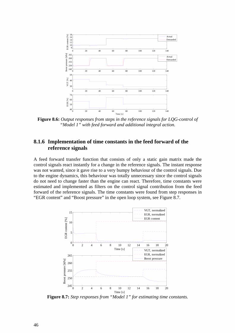
46

0 20 40 60 80 100 120 1408

1012141618

EGR

cont

ent [

%]

ActualDemanded

0 20 40 60 80 100 120 140245250

255

260265

Boos

t pre

ssur

e [k

Pa]

ActualDemanded

0 20 40 60 80 100 120 140

30

40

50

VG

T [%

]

0 20 40 60 80 100 120 14040

50

60

70

EGR

[%]

Time [s] Figure 8.6: Output responses from steps in the reference signals for LQG-control of

“Model 1” with feed forward and additional integral action.

8.1.6 Implementation of time constants in the feed forward of the

reference signals A feed forward transfer function that consists of only a static gain matrix made the control signals react instantly for a change in the reference signals. The instant response was not wanted, since it gave rise to a very bumpy behaviour of the control signals. Due to the engine dynamics, this behaviour was totally unnecessary since the control signals do not need to change faster than the engine can react. Therefore, time constants were estimated and implemented as filters on the control signal contribution from the feed forward of the reference signals. The time constants were found from step responses in “EGR content” and “Boost pressure” in the open loop system, see Figure 8.7.

0 2 4 6 8 10 12 14 16 18 200

5

10

15

Time [s]

EGR

cont

ent [

%]

VGT, normalizedEGR, normalizedEGR content

0 2 4 6 8 10 12 14 16 18 20245

250

255

260

265

Time [s]

Boos

t pre

ssur

e [k

Pa]

VGT, normalizedEGR, normalizedBoost pressure

Figure 8.7: Step responses from “Model 1” for estimating time constants.

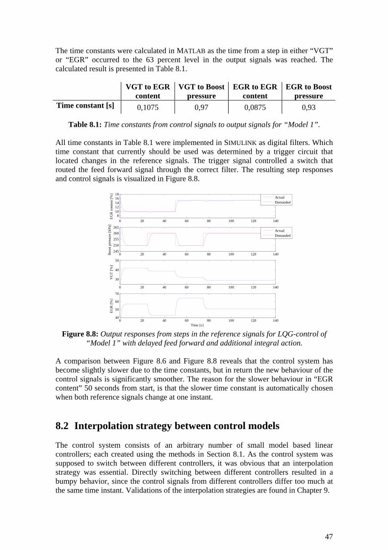
47

The time constants were calculated in MATLAB as the time from a step in either “VGT” or “EGR” occurred to the 63 percent level in the output signals was reached. The calculated result is presented in Table 8.1.

VGT to EGR content

VGT to Boost pressure

EGR to EGR content

EGR to Boost pressure

Time constant [s] 0,1075 0,97 0,0875 0,93

Table 8.1: Time constants from control signals to output signals for “Model 1”. All time constants in Table 8.1 were implemented in SIMULINK as digital filters. Which time constant that currently should be used was determined by a trigger circuit that located changes in the reference signals. The trigger signal controlled a switch that routed the feed forward signal through the correct filter. The resulting step responses and control signals is visualized in Figure 8.8.

0 20 40 60 80 100 120 1408

1012141618

EGR

cont

ent [

%]

ActualDemanded

0 20 40 60 80 100 120 140245250

255

260265

Boos

t pre

ssur

e [k

Pa]

ActualDemanded

0 20 40 60 80 100 120 140

30

40

50

VG

T [%

]

0 20 40 60 80 100 120 14040

50

60

70

EGR

[%]

Time [s] Figure 8.8: Output responses from steps in the reference signals for LQG-control of

“Model 1” with delayed feed forward and additional integral action.

A comparison between Figure 8.6 and Figure 8.8 reveals that the control system has become slightly slower due to the time constants, but in return the new behaviour of the control signals is significantly smoother. The reason for the slower behaviour in “EGR content” 50 seconds from start, is that the slower time constant is automatically chosen when both reference signals change at one instant. 8.2 Interpolation strategy between control models The control system consists of an arbitrary number of small model based linear controllers; each created using the methods in Section 8.1. As the control system was supposed to switch between different controllers, it was obvious that an interpolation strategy was essential. Directly switching between different controllers resulted in a bumpy behavior, since the control signals from different controllers differ too much at the same time instant. Validations of the interpolation strategies are found in Chapter 9.

48

8.2.1 Time based interpolation method To smoothly go from one controller to another, a time based interpolation strategy was developed. A look-up table with VGT on the x-axis and EGR on the y-axis was used in order to decide the preferred model to use by the controller at all time instants. A memory circuit was used in order to remember the previous model when the demand model changed. Changes in the demand signal did also trig an interpolation between the demanded model output signals and the previous model outputs. The interpolation lasted for a fixed amount of time. In order to prevent bumps, the interpolation method was not allowed to switch control model before the previous interpolation was finished. Therefore, the actual model might not always be equal to the demanded model. To prevent wind-up of the integral states, the control error signals to the integral action were linearly weighted during the interpolation process. The weight for one model was equal to one when only that model was used, and zero when purely the other model was used. The integral states were adjusted to zero in all control models when their corresponding weight was zero. 8.2.2 Fraction based interpolation method The fraction based interpolation strategy was such that up to four different controllers could operate at the same time. In the interpolation strategy for the combined engine model, the four models were chosen from the control signals. This method was not preferable in the controller interpolation strategy, since it resulted in an algebraic loop. In order to prevent this loop, the control signals had to be delayed, which resulted in oscillations in the closed loop system. Therefore, the controllers currently in use were chosen to depend on the reference signals instead and the operating point in “Speed” and “Torque”. To find out which controllers to currently use, one table was created in MATLAB for each combination of “Speed” and “Torque” with “EGR content” on the x-axis and “Boost pressure” on the y-axis. Only one table was required, since this thesis focuses on just one combination of “Speed” and “Torque”. The table was built from quadrates with controller numbers in the same way as for the combined engine model, see Section 7.1. In order to prevent wind-up of the integral states, the control error signals to the integral action were always weighted with the model weights. Adjustment of the integral states in all control models that were not currently in use was made in the same way as for the time based interpolation method.

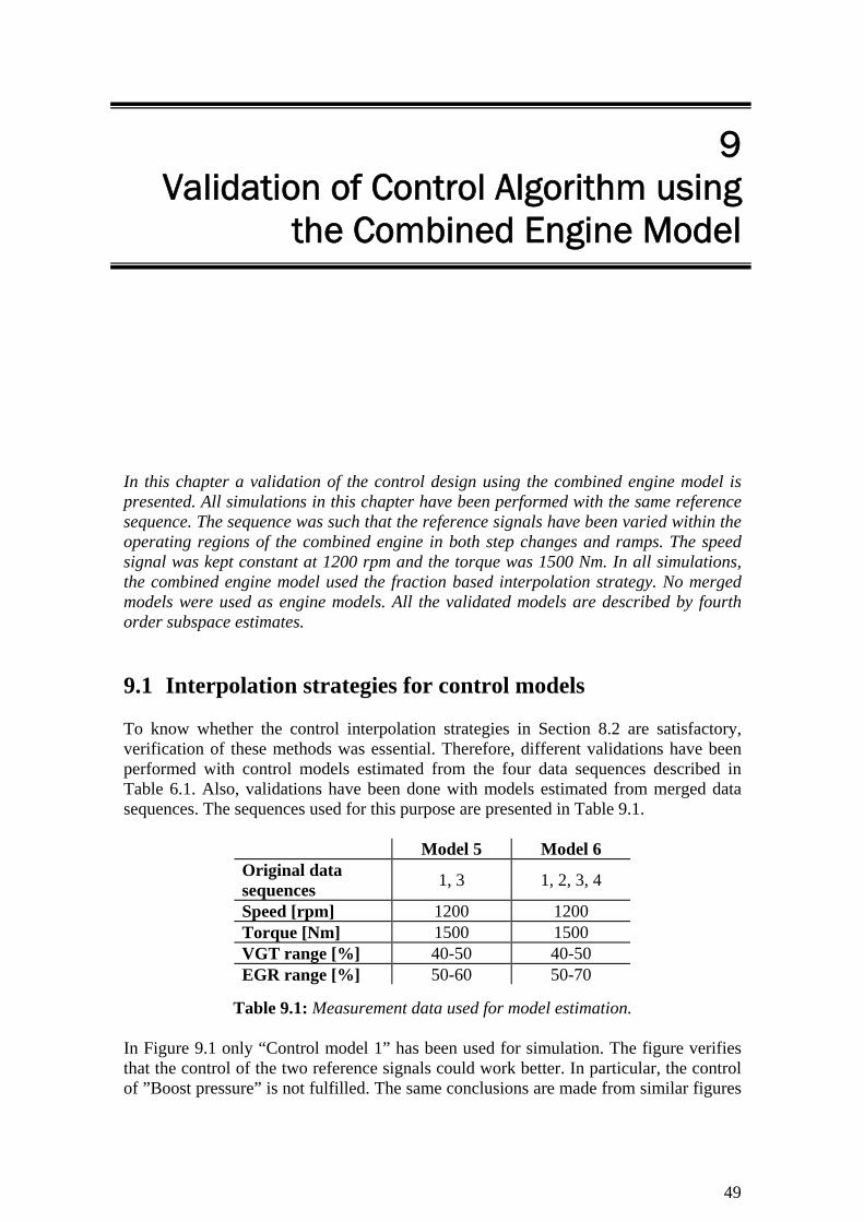
49

9 Validation of Control Algorithm using

the Combined Engine Model In this chapter a validation of the control design using the combined engine model is presented. All simulations in this chapter have been performed with the same reference sequence. The sequence was such that the reference signals have been varied within the operating regions of the combined engine in both step changes and ramps. The speed signal was kept constant at 1200 rpm and the torque was 1500 Nm. In all simulations, the combined engine model used the fraction based interpolation strategy. No merged models were used as engine models. All the validated models are described by fourth order subspace estimates. 9.1 Interpolation strategies for control models To know whether the control interpolation strategies in Section 8.2 are satisfactory, verification of these methods was essential. Therefore, different validations have been performed with control models estimated from the four data sequences described in Table 6.1. Also, validations have been done with models estimated from merged data sequences. The sequences used for this purpose are presented in Table 9.1.

Model 5 Model 6 Original data sequences 1, 3 1, 2, 3, 4

Speed [rpm] 1200 1200 Torque [Nm] 1500 1500 VGT range [%] 40-50 40-50 EGR range [%] 50-60 50-70

Table 9.1: Measurement data used for model estimation.

In Figure 9.1 only “Control model 1” has been used for simulation. The figure verifies that the control of the two reference signals could work better. In particular, the control of ”Boost pressure” is not fulfilled. The same conclusions are made from similar figures

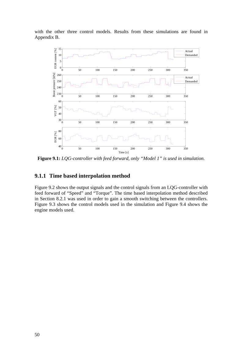
50

with the other three control models. Results from these simulations are found in Appendix B.

0 50 100 150 200 250 300 3500

5

10

15

EGR

cont

ent [

%]

ActualDemanded

0 50 100 150 200 250 300 350230

240

250

260

Boos

t pre

ssur

e [k

Pa]

ActualDemanded

0 50 100 150 200 250 300 35030

40

50

60

VG

T [%

]

0 50 100 150 200 250 300 35040

60

80

EGR

[%]

Time [s] Figure 9.1: LQG-controller with feed forward, only “Model 1” is used in simulation.

9.1.1 Time based interpolation method Figure 9.2 shows the output signals and the control signals from an LQG-controller with feed forward of “Speed” and “Torque”. The time based interpolation method described in Section 8.2.1 was used in order to gain a smooth switching between the controllers. Figure 9.3 shows the control models used in the simulation and Figure 9.4 shows the engine models used.

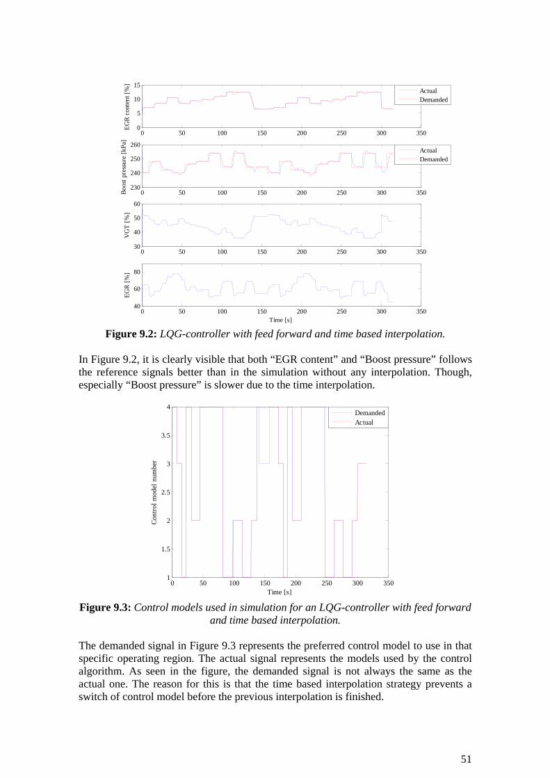
51

0 50 100 150 200 250 300 3500

5

10

15

EGR

cont

ent [

%]

ActualDemanded

0 50 100 150 200 250 300 350230

240

250

260

Boos

t pre

ssur

e [k

Pa]

ActualDemanded

0 50 100 150 200 250 300 35030

40

50

60

VG

T [%

]

0 50 100 150 200 250 300 35040

60

80

EGR

[%]

Time [s] Figure 9.2: LQG-controller with feed forward and time based interpolation.

In Figure 9.2, it is clearly visible that both “EGR content” and “Boost pressure” follows the reference signals better than in the simulation without any interpolation. Though, especially “Boost pressure” is slower due to the time interpolation.

0 50 100 150 200 250 300 3501

1.5

2

2.5

3

3.5

4

Time [s]

Cont

rol m

odel

num

ber

DemandedActual

Figure 9.3: Control models used in simulation for an LQG-controller with feed forward

and time based interpolation.

The demanded signal in Figure 9.3 represents the preferred control model to use in that specific operating region. The actual signal represents the models used by the control algorithm. As seen in the figure, the demanded signal is not always the same as the actual one. The reason for this is that the time based interpolation strategy prevents a switch of control model before the previous interpolation is finished.

52

0 50 100 150 200 250 300 3500

2

4

FractionModel

0 50 100 150 200 250 300 3500

2

4

En

gine

mod

el n

umbe

r

FractionModel

0 50 100 150 200 250 300 3500

2

4

Engi

ne m

odel

frac

tion,

FractionModel

0 50 100 150 200 250 300 3500

2

4

Time [s]

FractionModel

Figure 9.4: Engine models used in simulation for an LQG-controller with feed forward

and time based interpolation. In Figure 9.4 the engine models used for the simulation are shown. The four subplots represent the corners in the quadrate described in Section 7.1.1. In each subplot, the current engine model for that specific corner is showed and also the fraction which describes how much of that model that is used for interpolation. 9.1.2 Fraction based interpolation method In Figure 9.5 the output and the control signals from an LQG-controller with feed forward of “Speed” and “Torque” is seen. The interpolation control strategy uses all four individual state-space models. The control models used during simulation are visualized in Figure 9.6 and the different engine models are shown in Figure 9.7. An acceptable output as a result of the control interpolation approach is verified in Figure 9.5. The gain of the control strategy, which means usage of different control models for different operating regions, is clearly seen. The control signals appear to be smooth except for the spikes in the “EGR” signal. These spikes are thus identified to be a result of the output from the engine models. In Figure 7.5, an overshoot is seen after 10 s for all four models. This is due to the same phenomena as the one that occur in this simulation. The resulting overshoot from the engine models in “EGR content” affects the control in such way that spikes occur in the “EGR” signal.

53

0 50 100 150 200 250 300 3500

5

10

15

EGR

cont

ent [

%]

ActualDemanded

0 50 100 150 200 250 300 350230

240

250

260

Boos

t pre

ssur

e [k

Pa]

ActualDemanded

0 50 100 150 200 250 300 35030

40

50

60

VG

T [%

]

0 50 100 150 200 250 300 35040

60

80

EGR

[%]

Time [s] Figure 9.5: LQG-controller with feed forward and fraction based interpolation.

0 50 100 150 200 250 300 3500

2

4

FractionModel

0 50 100 150 200 250 300 3500

2

4

C

ontro

l mod

el n

umbe

r

FractionModel

0 50 100 150 200 250 300 3500

2

4

Cont

rol m

odel

frac

tion,

FractionModel

0 50 100 150 200 250 300 3500

2

4

Time [s]

FractionModel

Figure 9.6: Control models used in simulation for an LQG-controller with feed forward

and fraction based interpolation. In Figure 9.6, the four subplots represent the corners in the model quadrate for the control models. The reference signals have been chosen in such way that the interpolation strategy for the control models operated at the boundary of the model quadrate, in the upper left corner. Therefore, the weights of the other corners are equal to zero in steady state operation.

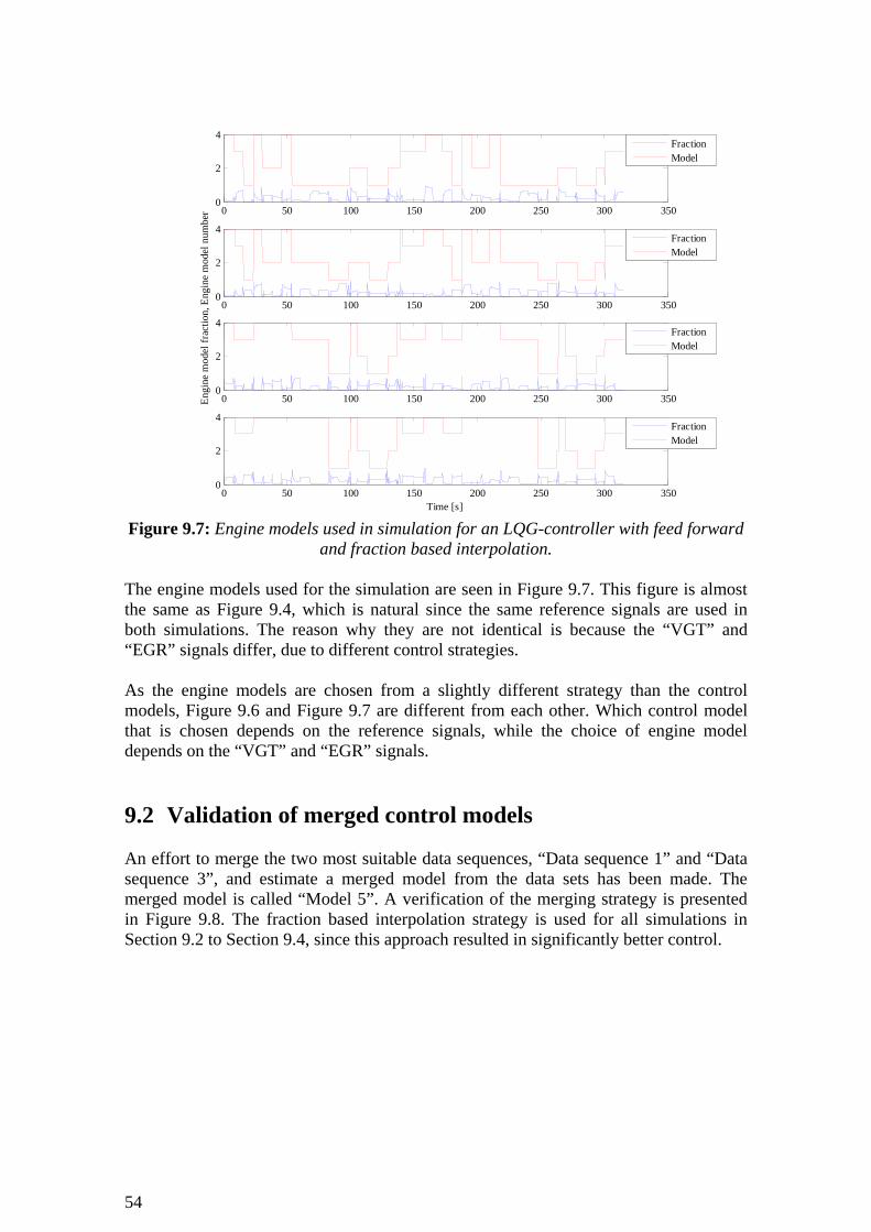
54

0 50 100 150 200 250 300 3500

2

4

FractionModel

0 50 100 150 200 250 300 3500

2

4

En

gine

mod

el n

umbe

r

FractionModel

0 50 100 150 200 250 300 3500

2

4

Engi

ne m

odel

frac

tion,

FractionModel

0 50 100 150 200 250 300 3500

2

4

Time [s]

FractionModel

Figure 9.7: Engine models used in simulation for an LQG-controller with feed forward

and fraction based interpolation.

The engine models used for the simulation are seen in Figure 9.7. This figure is almost the same as Figure 9.4, which is natural since the same reference signals are used in both simulations. The reason why they are not identical is because the “VGT” and “EGR” signals differ, due to different control strategies. As the engine models are chosen from a slightly different strategy than the control models, Figure 9.6 and Figure 9.7 are different from each other. Which control model that is chosen depends on the reference signals, while the choice of engine model depends on the “VGT” and “EGR” signals. 9.2 Validation of merged control models An effort to merge the two most suitable data sequences, “Data sequence 1” and “Data sequence 3”, and estimate a merged model from the data sets has been made. The merged model is called “Model 5”. A verification of the merging strategy is presented in Figure 9.8. The fraction based interpolation strategy is used for all simulations in Section 9.2 to Section 9.4, since this approach resulted in significantly better control.

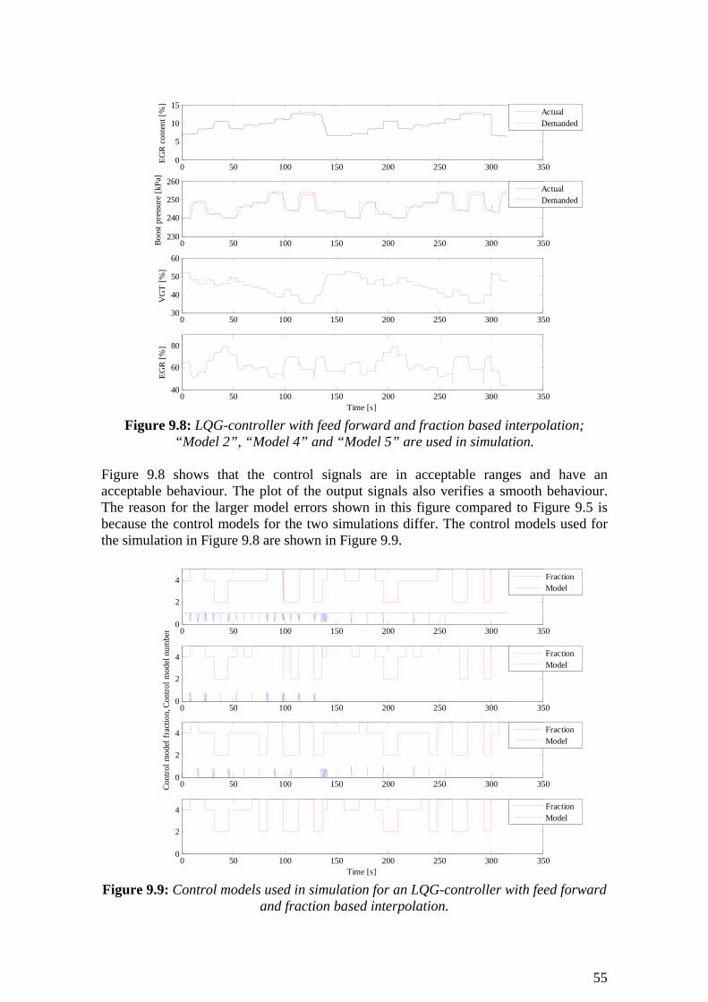
55

0 50 100 150 200 250 300 3500

5

10

15

EGR

cont

ent [

%]

ActualDemanded

0 50 100 150 200 250 300 350230

240

250

260

Boos

t pre

ssur

e [k

Pa]

ActualDemanded

0 50 100 150 200 250 300 35030

40

50

60

VG

T [%

]

0 50 100 150 200 250 300 35040

60

80

EGR

[%]

Time [s] Figure 9.8: LQG-controller with feed forward and fraction based interpolation;

“Model 2”, “Model 4” and “Model 5” are used in simulation. Figure 9.8 shows that the control signals are in acceptable ranges and have an acceptable behaviour. The plot of the output signals also verifies a smooth behaviour. The reason for the larger model errors shown in this figure compared to Figure 9.5 is because the control models for the two simulations differ. The control models used for the simulation in Figure 9.8 are shown in Figure 9.9.

0 50 100 150 200 250 300 3500

2

4

FractionModel

0 50 100 150 200 250 300 3500

2

4

C

ontro

l mod

el n

umbe

r

FractionModel

0 50 100 150 200 250 300 3500

2

4

Cont

rol m

odel

frac

tion,

FractionModel

0 50 100 150 200 250 300 3500

2

4

Time [s]

FractionModel

Figure 9.9: Control models used in simulation for an LQG-controller with feed forward

and fraction based interpolation.

56

In Figure 9.9 it is seen that the merged model estimated from “Data sequence 1” and “Data sequence 3” has been used for the periods where the larger model errors are observed. It is clear that “Model 5” does not capture the engine dynamics as good as “Model 1” and “Model 3” does when they are used instead.

0 50 100 150 200 250 300 3500

2

4

FractionModel

0 50 100 150 200 250 300 3500

2

4

En

gine

mod

el n

umbe

r

FractionModel

0 50 100 150 200 250 300 3500

2

4

Engi

ne m

odel

frac

tion,

FractionModel

0 50 100 150 200 250 300 3500

2

4

Time [s]

FractionModel

Figure 9.10: Engine models used in simulation for an LQG-controller with feed

forward and fraction based interpolation. Figure 9.10 shows the engine models used for the simulation in Figure 9.8. It is seen that the used engine models differ slightly from the simulation with no merged control models in Figure 9.7. An attempt to merge all four data sequences and estimate one model from these data has been made. The estimate is named “Model 6”. The output result from simulation with an LQG-controller with feed forward of “Speed” and “Torque” is seen in Figure 9.11.

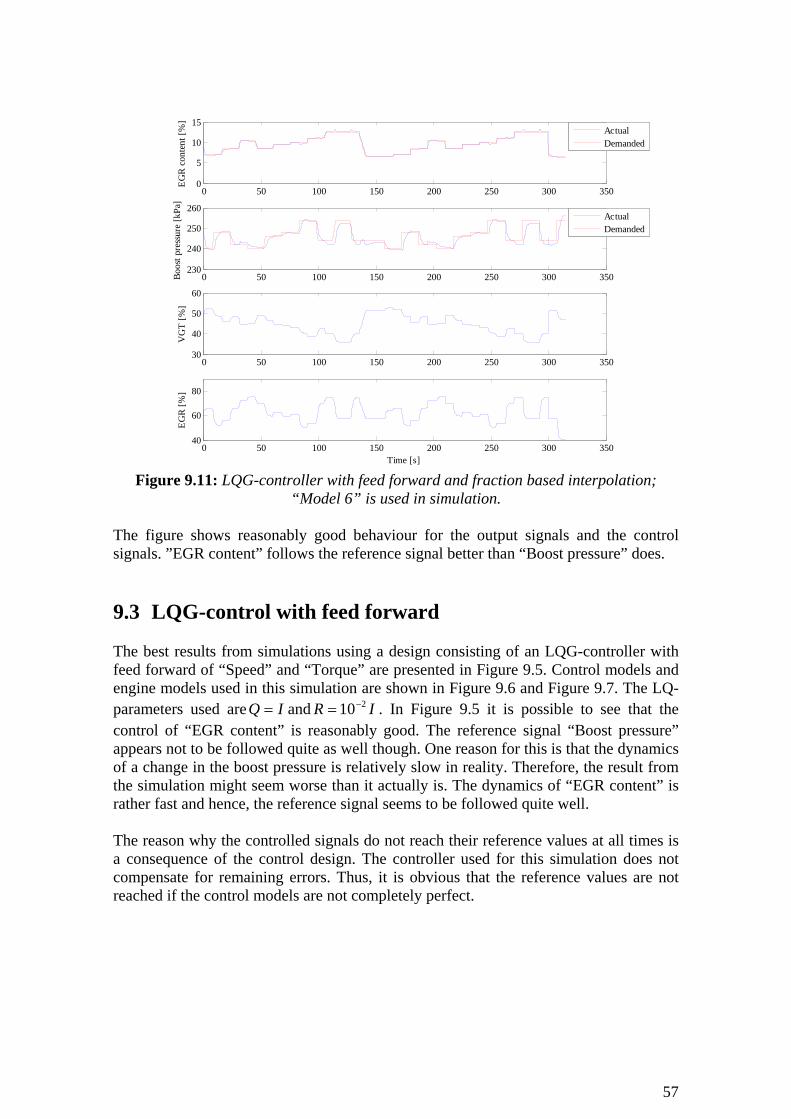
57

0 50 100 150 200 250 300 3500

5

10

15

EGR

cont

ent [

%]

ActualDemanded

0 50 100 150 200 250 300 350230

240

250

260

Boos

t pre

ssur

e [k

Pa]

ActualDemanded

0 50 100 150 200 250 300 35030

40

50

60

VG

T [%

]

0 50 100 150 200 250 300 35040

60

80

EGR

[%]

Time [s] Figure 9.11: LQG-controller with feed forward and fraction based interpolation;

“Model 6” is used in simulation. The figure shows reasonably good behaviour for the output signals and the control signals. ”EGR content” follows the reference signal better than “Boost pressure” does. 9.3 LQG-control with feed forward The best results from simulations using a design consisting of an LQG-controller with feed forward of “Speed” and “Torque” are presented in Figure 9.5. Control models and engine models used in this simulation are shown in Figure 9.6 and Figure 9.7. The LQ-parameters used are IQ = and IR 210−= . In Figure 9.5 it is possible to see that the control of “EGR content” is reasonably good. The reference signal “Boost pressure” appears not to be followed quite as well though. One reason for this is that the dynamics of a change in the boost pressure is relatively slow in reality. Therefore, the result from the simulation might seem worse than it actually is. The dynamics of “EGR content” is rather fast and hence, the reference signal seems to be followed quite well. The reason why the controlled signals do not reach their reference values at all times is a consequence of the control design. The controller used for this simulation does not compensate for remaining errors. Thus, it is obvious that the reference values are not reached if the control models are not completely perfect.

58

9.4 LQG-control with feed forward and additional integral action

In this section the complete control design described in this master thesis is validated. The results from simulation presented in Figure 9.12 are obtained for an LQG-controller with feed forward of “Speed” and “Torque” and additional integral action. The LQ-parameters used for the control design are found in (9.1).

IRIQ NoIntNoInt210−==

(9.1)

IRQ 2

5

5

10

10000000100000001000000100000010000001

−

−

−

=

⎥⎥⎥⎥⎥⎥⎥⎥

⎦

⎤

⎢⎢⎢⎢⎢⎢⎢⎢

⎣

⎡

=

Figure 9.12 shows that the reference signals are followed quite well, especially “EGR content” seems to be at a good level most of the time. “Boost pressure” seems to have greater overshoots and the reference is not always followed. It is important to keep in mind that the relative overshoots are not huge compared to the changes in the reference signals. The overshoots are a result of the integral action. When the control signal contribution from the additional integral action is increased, the trade off is a greater overshoot. Both control signals are at acceptable levels and have a smooth behavior.

0 50 100 150 200 250 300 3500

5

10

15

EGR

cont

ent [

%]

ActualDemanded

0 50 100 150 200 250 300 350230

240

250

260

Boos

t pre

ssur

e [k

Pa]

ActualDemanded

0 50 100 150 200 250 300 35030

40

50

60

VG

T [%

]

0 50 100 150 200 250 300 35040

60

80

EGR

[%]

Time [s] Figure 9.12: Simulation using an LQG-controller with feed forward, additional integral

action and fraction based interpolation.

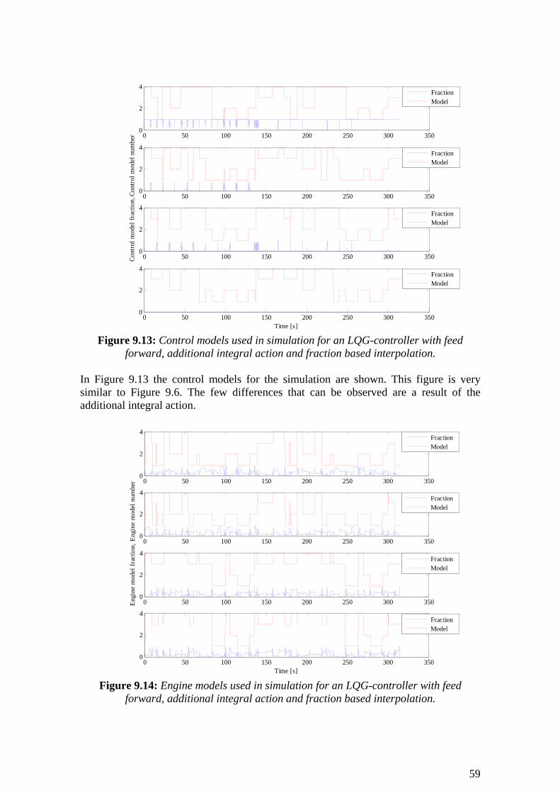
59

0 50 100 150 200 250 300 3500

2

4

FractionModel

0 50 100 150 200 250 300 3500

2

4

C

ontro

l mod

el n

umbe

r

FractionModel

0 50 100 150 200 250 300 3500

2

4

Cont

rol m

odel

frac

tion,

FractionModel

0 50 100 150 200 250 300 3500

2

4

Time [s]

FractionModel

Figure 9.13: Control models used in simulation for an LQG-controller with feed

forward, additional integral action and fraction based interpolation. In Figure 9.13 the control models for the simulation are shown. This figure is very similar to Figure 9.6. The few differences that can be observed are a result of the additional integral action.

0 50 100 150 200 250 300 3500

2

4

FractionModel

0 50 100 150 200 250 300 3500

2

4

En

gine

mod

el n

umbe

r

FractionModel

0 50 100 150 200 250 300 3500

2

4

Engi

ne m

odel

frac

tion,

FractionModel

0 50 100 150 200 250 300 3500

2

4

Time [s]

FractionModel

Figure 9.14: Engine models used in simulation for an LQG-controller with feed

forward, additional integral action and fraction based interpolation.

60

Figure 9.14 presents the engine models used for the simulation. A comparison between this figure and Figure 9.7 confirms that the two figures are different. The differences in engine models are due to slightly different control signals used for the two simulations. This is thus a result of the additional integral action.

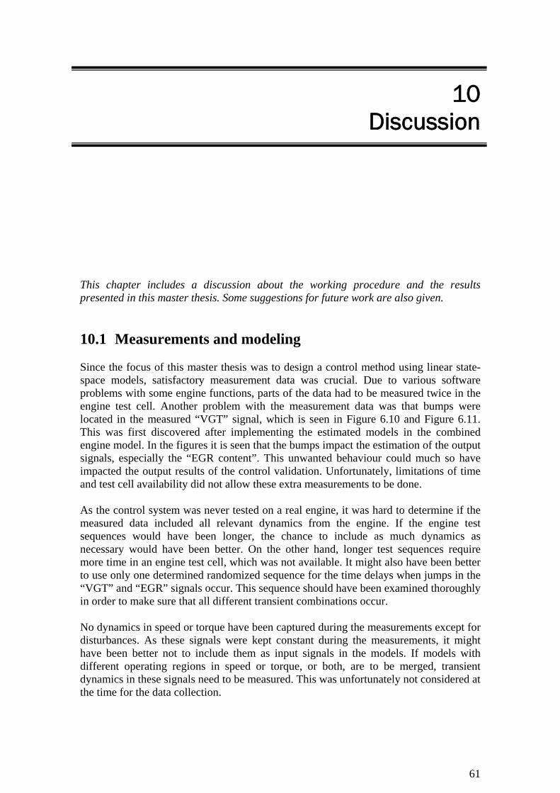
61

10 Discussion

This chapter includes a discussion about the working procedure and the results presented in this master thesis. Some suggestions for future work are also given. 10.1 Measurements and modeling Since the focus of this master thesis was to design a control method using linear state-space models, satisfactory measurement data was crucial. Due to various software problems with some engine functions, parts of the data had to be measured twice in the engine test cell. Another problem with the measurement data was that bumps were located in the measured “VGT” signal, which is seen in Figure 6.10 and Figure 6.11. This was first discovered after implementing the estimated models in the combined engine model. In the figures it is seen that the bumps impact the estimation of the output signals, especially the “EGR content”. This unwanted behaviour could much so have impacted the output results of the control validation. Unfortunately, limitations of time and test cell availability did not allow these extra measurements to be done. As the control system was never tested on a real engine, it was hard to determine if the measured data included all relevant dynamics from the engine. If the engine test sequences would have been longer, the chance to include as much dynamics as necessary would have been better. On the other hand, longer test sequences require more time in an engine test cell, which was not available. It might also have been better to use only one determined randomized sequence for the time delays when jumps in the “VGT” and “EGR” signals occur. This sequence should have been examined thoroughly in order to make sure that all different transient combinations occur. No dynamics in speed or torque have been captured during the measurements except for disturbances. As these signals were kept constant during the measurements, it might have been better not to include them as input signals in the models. If models with different operating regions in speed or torque, or both, are to be merged, transient dynamics in these signals need to be measured. This was unfortunately not considered at the time for the data collection.

62

Merging models with satisfactory result was much harder than expected. A merge of models with slightly different dynamics resulted in poor reproduction of the measured engine output signals. In order to merge models with different speed and/or torque, dynamics for these signals is necessary. It would probably also be required to measure data for more than just six combinations of speed and torque due to nonlinearities. 10.2 The Combined engine model At start for this project all parts involved believed that there was a proper engine model at hand for simulation matters. However, this was to be a great issue later on in the project. In order to thoroughly evaluate the state-space models described in Chapter 6, the realization was that the control design had to be implemented in SIMULINK. To achieve this, a proper engine model was necessary. When reaching this far in the process it was obvious that no proper engine model was available at this stage. A physical engine model was about to be designed, but it was not yet calibrated for the same type of engine used when collecting data from the real test cell. Also, the model in itself was not verified or tested and it came clear that it had some issues to be dealt with, before it could be applied in any work at all. In order to move forward with the project, the decision was made to use system identification as a tool for designing an engine model. However, this was to be a huge limitation of the future process. The operating region of the engine was dramatically minimized and therefore the state-space models could never be fully validated. In order to do a better validation, several more measurements from an engine test cell would have been necessary. The simple time interpolation method presented in Section 8.2.1 for the control design, was never applied to the combined engine model. The reasons for this were both lack of time and also that this method was already validated in the control algorithm, where it caused significantly worse result than the fraction based interpolation method. Using the time and fraction based interpolation method gave rise to slightly better results than the fraction based interpolation method. Though, dual interpolation methods require significantly more computer power and therefore, the enhancement was probably not beneficial and was never tested in the combined engine model. 10.3 Control design An LQG-controller was chosen in order to control the combined engine. Of course, there are other linear multivariable model based controllers available. Though, two separate one dimensional controllers would not have been able to follow the reference signals, due to large cross coupling effects on the outputs from the control signals. When implementing additional integral action in the control algorithm, direct use of the new optimal gain matrix resulted in very large control signal contributions from the integral action. This problem could probably have been solved by adjusting the parameters in the R and Q matrices, something which was not done. Instead, the method described in Section 8.1.4 was used and it gave a better result with less time spent, since

63

the parameters regarding additional integral action could be adjusted independently of the rest of the control system. Other interpolation methods than described in Section 8.2, such as polynomial interpolation for instance, are of course available. Though, the intended regions were considered small enough for linear interpolation to be sufficient. 10.4 Validation of control algorithm on engine model From Section 8.1.2, it was obvious that feed forward of “Speed” and “Torque” was required in order to follow the reference signals sufficiently well. Though, it is not that obvious that additional integral action is desired for control of a real engine. It did improve the controller, but the result was not significantly better than with just feed forward of “Speed” and “Torque”. Additional integral action requires slightly more computer power due to calculation of the integral states. However, if the integral action is not implemented, stationary errors might not be handled. Stationary errors will for example occur due to dissimilarities between the models and the real engine. A merge of many models will probably also result in bad control due to model errors, if integral action is missing. When both additional integral action and feed forward of speed and torque were used in the control algorithm, some spikes were still left in the output signals, see Figure 9.12. This behavior was found to originate from the engine model, and it was not caused by the engine interpolation strategy. Since the control algorithm have not been validated on a real engine, it was hard to know if this behavior was to be expected or not. The time and fraction based interpolation method described in Section 7.1.2, could probably have been applied to the control system as well. It was thus never tried in this thesis work, mainly due to lack of time. If this method was to be implemented, anti-wind-up of the additional integral action during time interpolation would probably have been needed. 10.5 Future work In order to proceed with the multidimensional model based control of air and EGR into a diesel engine, designing a proper engine model is essential. Otherwise, the only way of fully validating the control algorithm is applying it to the real engine. New measurements in the engine test cell, including speed and torque dynamics, are crucial in order to increase the operating region for the control system. This would probably allow models from different speed and/or torque regions to be merged with satisfactory result. Better designed test sequences for the jumps in the VGT and EGR valve positions are preferred, in order to make sure that all dynamics will be caught. An LQ-controller is one of many multidimensional controllers. Other model based controllers might also be tested and compared to the LQ-controller. Since both control signals have nonlinear influence on the output signals, a nonlinear model and a nonlinear controller could probably provide good results.

64

65

11 Conclusions

The VGT and EGR actuators can be controlled using a model based control design, consisting of several linear controllers. As the VGT and the EGR valve both have very non linear physics, a huge amount of linear models was needed in order to give a good representation of the engine. Though, no proper engine model was available for validation and therefore, only a small part of the working region was examined. Measured data from experiments in the engine test cell was satisfactory for the small operating region. If the operating region is to be enlarged, new data including variations in speed and/or torque is essential. Linear subspace models of order four were considered to be the best choice. Merging of models could be done with satisfactory result if the models had similar dynamics. However, merging of models with different dynamics resulted in bad representation of the real engine. To control the engine model, a multivariable LQG controller with additional feed forward of “Speed” and “Torque” was required before any satisfactory results were achieved. This control system was sufficient as long as no model errors were introduced. If the controller used a model that differed significantly from the engine model, additional integral action was required in order to compensate for stationary errors. Model errors occurred during interpolation between different models in the controller and in the combined engine model, since different fraction based interpolation methods were used. Fraction based interpolation methods were considered to be the best choice for both the combined engine model and for the control strategy. The LQG-controller gave the best results of the control of the combined engine model when both feed forward of speed and torque and additional integral action was implemented. The control of the combined engine model was considered to be satisfactory for this control setup, especially when the control models were created from single data sequences. Though, merging two similar models resulted in sufficiently good control. Merging of all four investigated models resulted in significantly worse control, since the model dynamics differed too much. In order to compensate for these model errors, a stronger integral action would have been required. Thus, this was hard to achieve, since stronger integral action resulted in oscillations.

66

67

Bibliography Glad, T., Ljung, L. 2003. Reglerteori: Flervariabla och olinjära metoder, 2:a upplagan. Lund: Studentlitteratur., pp.144-149, 195-196, 270. Ljung, L. 1999. System Identification: Theory for the User, 2nd ed. Upper Saddle River: Prentice-Hall, Inc., pp.208-211, 460-465, 511-516. Ljung, L., Glad, T. 2004. Modellbygge och simulering, 2:a upplagan. Lund: Studentlitteratur., pp.279-285, 362. Schmidtbauer, B. 1999. Modellbaserade reglersystem. Lund: Studentlitteratur., p.168. The MATLAB Users Guide. (2006). The MathWorks, Inc., ARX Models, merge (idmodel) and resid. van Overschee, P., De Moor, B., 1996. Subspace Identification for Linear Systems: Theory – Implementation – Applications. Norwell: Kluwer Academic Publishers., pp.6-9. Åström, K. J., Wittenmark, B. 1997. Computer-Controlled Systems: Theory and Design, 3rd ed. Upper Saddle River: Prentice-Hall, Inc., pp.408-412.

68

69

A System Identification Validation

In this appendix results from the system identification validation is found. A.1 Different orders of ARX models

0 20 40 60 80 100 120 1406

8

10

12

EGR

cont

ent [

%]

Time [s]

0 20 40 60 80 100 120 140240

245

250

255

260

Boos

t pre

ssur

e [k

Pa]

Time [s]

Measured outputModel output

Measured outputModel output

Figure A.1: ARX model with 6 states, (na,nb,nk) = (1,1,1), compared with data from

measurements.

70

0 20 40 60 80 100 120 1406

8

10

12

EGR

cont

ent [

%]

Time [s]

0 20 40 60 80 100 120 140240

245

250

255

260

Boos

t pre

ssur

e [k

Pa]

Time [s]

Measured outputModel output

Measured outputModel output

Figure A.2: ARX model with 12 states, (na,nb,nk) = (2,2,1), compared with data from

measurements.

0 20 40 60 80 100 120 1406

8

10

12

EGR

cont

ent [

%]

Time [s]

0 20 40 60 80 100 120 140240

245

250

255

260

Boos

t pre

ssur

e [k

Pa]

Time [s]

Measured outputModel output

Measured outputModel output

Figure A.3: ARX model with 20 states, (na,nb,nk) = (4,3,1), compared with data from

measurements.

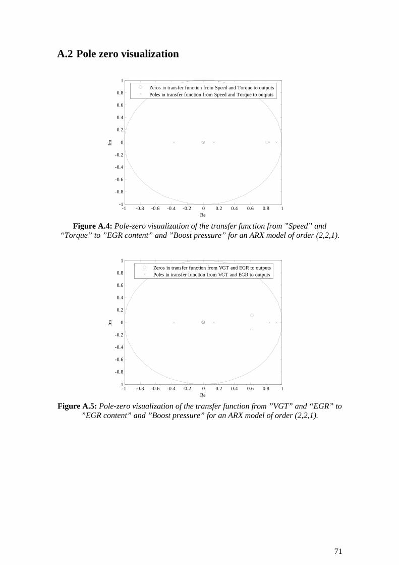
71

A.2 Pole zero visualization

-1 -0.8 -0.6 -0.4 -0.2 0 0.2 0.4 0.6 0.8 1-1

-0.8

-0.6

-0.4

-0.2

0

0.2

0.4

0.6

0.8

1

Re

Im

Zeros in transfer function from Speed and Torque to outputsPoles in transfer function from Speed and Torque to outputs

Figure A.4: Pole-zero visualization of the transfer function from ”Speed” and

“Torque” to ”EGR content” and ”Boost pressure” for an ARX model of order (2,2,1).

-1 -0.8 -0.6 -0.4 -0.2 0 0.2 0.4 0.6 0.8 1-1

-0.8

-0.6

-0.4

-0.2

0

0.2

0.4

0.6

0.8

1

Re

Im

Zeros in transfer function from VGT and EGR to outputsPoles in transfer function from VGT and EGR to outputs

Figure A.5: Pole-zero visualization of the transfer function from ”VGT” and “EGR” to

”EGR content” and ”Boost pressure” for an ARX model of order (2,2,1).

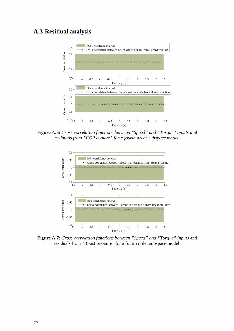
72

A.3 Residual analysis

-2.5 -2 -1.5 -1 -0.5 0 0.5 1 1.5 2 2.5-0.2

-0.1

0

0.1

0.2

Time lag [s]

Cros

s cor

rela

tion

-2.5 -2 -1.5 -1 -0.5 0 0.5 1 1.5 2 2.5-0.2

-0.1

0

0.1

0.2

Time lag [s]

Cros

s cor

rela

tion

99% confidence intervalCross correlation between Speed and residuals from Burned fraction

99% confidence intervalCross correlation between Torque and residuals from Burned fraction

Figure A.6: Cross correlation functions between ”Speed” and “Torque” inputs and

residuals from ”EGR content” for a fourth order subspace model.

-2.5 -2 -1.5 -1 -0.5 0 0.5 1 1.5 2 2.5-0.1

-0.05

0

0.05

0.1

Time lag [s]

Cros

s cor

rela

tion

-2.5 -2 -1.5 -1 -0.5 0 0.5 1 1.5 2 2.5-0.1

-0.05

0

0.05

0.1

Time lag [s]

Cros

s cor

rela

tion

99% confidence intervalCross correlation between Torque and residuals from Boost pressure

99% confidence intervalCross correlation between Speed and residuals from Boost pressure

Figure A.7: Cross correlation functions between ”Speed” and “Torque” inputs and

residuals from ”Boost pressure” for a fourth order subspace model.

73

A.4 Merging of models

10-3

10-2

10-1

100

101

102

10-3

10-2

10-1

Am

plitu

de

Frequency [rad/s]

10-3

10-2

10-1

100

101

102

-200

-100

0

100

Phas

e [d

eg]

Frequency [rad/s]

Frequency response from Model 1Frequency response from Model 3Frequency response from Merged model

10-3

10-2

10-1

100

101

102

10-4

10-2

100

Am

plitu

de

Frequency [rad/s]

10-3

10-2

10-1

100

101

102

-400

-200

0

200

Phas

e [d

eg]

Frequency [rad/s]

Frequency response from Model 1Frequency response from Model 3Frequency response from Merged model

Figure A.8: Bode diagram of the transfer function from ”Speed” to ”EGR content” (left) and ”Boost pressure” (right). The plots are for outputs from “Model 1” and

“Model 3”, together with a merged model, for fourth order estimates.

10-3

10-2

10-1

100

101

102

10-4

10-3

10-2

10-1

Am

plitu

de

Frequency [rad/s]

10-3

10-2

10-1

100

101

102

-100

0

100

200

300

Phas

e [d

eg]

Frequency [rad/s]

Frequency response from Model 1Frequency response from Model 3Frequency response from Merged model

10-3

10-2

10-1

100

101

102

10-3

10-2

10-1

100

Am

plitu

de

Frequency [rad/s]

10-3

10-2

10-1

100

101

102

-200

-150

-100

-50

0

Phas

e [d

eg]

Frequency [rad/s]

Frequency response from Model 1Frequency response from Model 3Frequency response from Merged model

Figure A.9: Bode diagram of the transfer function from “Torque” to ”EGR content”

(left) and ”Boost pressure” (right). The plots are for outputs from “Model 1” and “Model 3”, together with a merged model, for fourth order estimates.

74

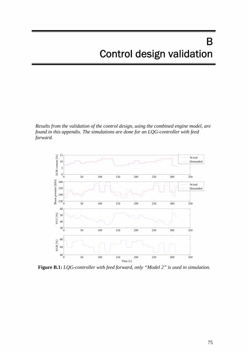
75

B Control design validation

Results from the validation of the control design, using the combined engine model, are found in this appendix. The simulations are done for an LQG-controller with feed forward.

0 50 100 150 200 250 300 3500

5

10

15

EGR

cont

ent [

%]

ActualDemanded

0 50 100 150 200 250 300 350230

240

250

260

Boos

t pre

ssur

e [k

Pa]

ActualDemanded

0 50 100 150 200 250 300 35030

40

50

60

VG

T [%

]

0 50 100 150 200 250 300 35040

60

80

EGR

[%]

Time [s] Figure B.1: LQG-controller with feed forward, only “Model 2” is used in simulation.

76

0 50 100 150 200 250 300 3500

5

10

15

EGR

cont

ent [

%]

ActualDemanded

0 50 100 150 200 250 300 350230

240

250

260

Boos

t pre

ssur

e [k

Pa]

ActualDemanded

0 50 100 150 200 250 300 35030

40

50

60

VG

T [%

]

0 50 100 150 200 250 300 35040

60

80

EGR

[%]

Time [s] Figure B.2: LQG-controller with feed forward, only “Model 3” is used in simulation.

0 50 100 150 200 250 300 3500

5

10

15

EGR

cont

ent [

%]

ActualDemanded

0 50 100 150 200 250 300 350230

240

250

260

Boos

t pre

ssur

e [k

Pa]

ActualDemanded

0 50 100 150 200 250 300 35030

40

50

60

VG

T [%

]

0 50 100 150 200 250 300 35040

60

80

EGR

[%]

Time [s] Figure B.3: LQG-controller with feed forward, only “Model 1” is used in simulation.